lecture 8. roy model, iv with essential heterogeneity,...
TRANSCRIPT

Introduction The Roy model Extended Roy model Generalized Roy model The MTE LATE
Lecture 8. Roy Model, IV with essentialheterogeneity, MTE
Economics 2123George Washington University
Instructor: Prof. Ben Williams

Introduction The Roy model Extended Roy model Generalized Roy model The MTE LATE
Heterogeneity
• When we talk about heterogeneity, usually we meanheterogeneity in causal effects.• The individual causal effect differs across individuals.
• James Heckman, among many others, has argued overthe past 30-40 years that this type of heterogeneity isprevalent.

Introduction The Roy model Extended Roy model Generalized Roy model The MTE LATE
Heterogeneity
• Recall the discussion from the first lecture:• Y1i − Y0i represents the individual treatment effect• δx = E(Y1i − Y0i | Xi = x) is the average treatment effect
conditional on x• observable heterogeneity is when δx varies with x
• under the conditional independence assumption, OLSestimates a weighted average,
∑x wxδx .
• note that this result allows for unobserved heterogeneity toobecause we do not assume that Y1i − Y0i = δXi .

Introduction The Roy model Extended Roy model Generalized Roy model The MTE LATE
Heterogeneity
• Recall the discussion from the first lecture:• Y1i − Y0i represents the individual treatment effect• δx = E(Y1i − Y0i | Xi = x) is the average treatment effect
conditional on x• observable heterogeneity is when δx varies with x• under the conditional independence assumption, OLS
estimates a weighted average,∑
x wxδx .
• note that this result allows for unobserved heterogeneity toobecause we do not assume that Y1i − Y0i = δXi .

Introduction The Roy model Extended Roy model Generalized Roy model The MTE LATE
Heterogeneity
• Recall the discussion from the first lecture:• Y1i − Y0i represents the individual treatment effect• δx = E(Y1i − Y0i | Xi = x) is the average treatment effect
conditional on x• observable heterogeneity is when δx varies with x• under the conditional independence assumption, OLS
estimates a weighted average,∑
x wxδx .• note that this result allows for unobserved heterogeneity too
because we do not assume that Y1i − Y0i = δXi .
Introduction The Roy model Extended Roy model Generalized Roy model The MTE LATE
Heterogeneity
• What if the conditional independence assumption fails?• we may use an instrumental variable strategy• if there is also heterogeneity, what does IV estimate?

Introduction The Roy model Extended Roy model Generalized Roy model The MTE LATE
Heterogeneity
• What if there is unobserved heterogeneity?• i.e., if Y1i − Y0i 6= δXi
• this could be ok• a textbook example:
• suppose Yi = α + βiDi + ui where βi = β + ηi
• then Yi = α + βDi + εi where εi = ui + ηiDi
• if E(uiDi ) = 0 and E(ηi | Di ) = 0 then OLS estimatesβ = E(βi )

Introduction The Roy model Extended Roy model Generalized Roy model The MTE LATE
Heterogeneity
• The Roy model will be used to demonstrate a link betweenunobserved heterogeneity and endogeneity.
• The textbook example above is misleading because oftenηi will be correlated with Di .
• Moreover, even if Zi is uncorrelated with ui it will often notbe uncorrelated with ηiDi .
Introduction The Roy model Extended Roy model Generalized Roy model The MTE LATE
Roy model
The Roy model is a model of comparative advantage:• Potential earnings in sectors 0 and 1: Y0,Y1
• Individuals choose sector 1 if and only if Y1 − Y0 ≥ cwhere c is a nonrandom cost.
• Heckman and Honore (1990) studied the empiricalimplications and identification of this model.

Introduction The Roy model Extended Roy model Generalized Roy model The MTE LATE
Roy model
The extended and generalized Roy model:• the extended model allows for an observable cost
component, D = 1(Y1 − Y0 ≥ c(Z )) where Z is a vector ofcovariates and c is a possibly unknown function.
• the generalized model allows for an unobservable costcomponent, D = 1(Y1 − Y0 ≥ c(Z ,V )) where V isunobservable

Introduction The Roy model Extended Roy model Generalized Roy model The MTE LATE
Roy model• In the Roy model, Yd = µd + Ud where E(Ud ) = 0 for
d = 0,1.• If we observe a vector of covariates X , µd = µd (X ).• Often µd (X ) = β′dX .• Now
Yi = Y0i + (Y1i − Y0i)Di
= µ0 + (Y1i − Y0i)Di + U0i
( = α + βi Di + ui)
• What the Roy model gives us is that it adds a model for Dto the potential outcomes framework and demonstrates theimportant link between the model for D and the model forthe potential outcomes.
Introduction The Roy model Extended Roy model Generalized Roy model The MTE LATE
Roy model
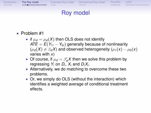
• Problem #1• if µd = µd (X ) then OLS does not identify
ATE = E(Y1i − Y0i ) generally because of nonlinearity(µd (X ) 6= βdX ) and observed heterogeneity (µ1(x)− µ0(x)varies with x)
• Of course, if µd = β′dX then we solve this problem byregressing Yi on Di , Xi and DiXi .
• Alternatively, we do matching to overcome these twoproblems.
• Or, we simply do OLS (without the interaction) whichidentifies a weighted average of conditional treatmenteffects.
Introduction The Roy model Extended Roy model Generalized Roy model The MTE LATE
Roy model
• Problem #1• if µd = µd (X ) then OLS does not identify
ATE = E(Y1i − Y0i ) generally because of nonlinearity(µd (X ) 6= βdX ) and observed heterogeneity (µ1(x)− µ0(x)varies with x)
• Of course, if µd = β′dX then we solve this problem byregressing Yi on Di , Xi and DiXi .
• Alternatively, we do matching to overcome these twoproblems.
• Or, we simply do OLS (without the interaction) whichidentifies a weighted average of conditional treatmenteffects.

Introduction The Roy model Extended Roy model Generalized Roy model The MTE LATE
Roy model
• Problem #2• The above solutions only work under the conditional
independence assumption, (Y0i ,Y1i ) ⊥⊥ Di | Xi .• In the generalized Roy model, this is only satisfied if
(U0i ,U1i ) ⊥⊥ (U1i − U0i ,Vi ) | Xi ,Zi
• no unobserved heterogeneity and non-random orindependent costs

Introduction The Roy model Extended Roy model Generalized Roy model The MTE LATE
Roy model
• Problem #2• A more general model is
D = 1(E(Y1 − Y0 − c(Z ,V ) | I) ≥ 0) where E(· | I)represents the expected value from the decision-maker’sperspective.
• In this case, conditional independence can be stated interms of the information available to the econometricianrelative to what’s available to the decision-maker.• What if I consists of X and Z but not U1i ,U0i or Vi?

Introduction The Roy model Extended Roy model Generalized Roy model The MTE LATE
Roy model
• Problem #2• Note also that Yi = µ0 + (µ1 − µ0)Di + U0i + (U1i − U0i )Di• There is a selection on unobservables problem (Di is
correlated with U0i ) and an unobserved heterogeneityproblem (U1i − U0i 6= 0).
• An exercise for you:• What happens if U1i = ∆i + U0i where ∆i is independent of
U0i?• What if U1i = U0i but U0i is not independent of Di (perhaps
because U0i is correlated with Vi )?
Introduction The Roy model Extended Roy model Generalized Roy model The MTE LATE
Roy model
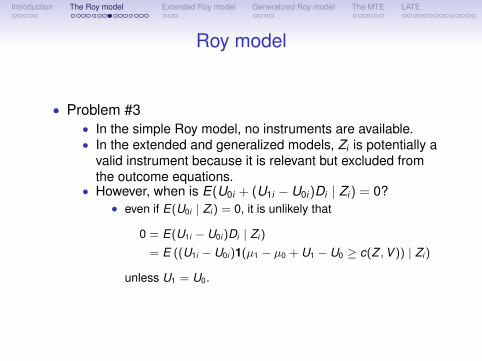
• Problem #3• In the simple Roy model, no instruments are available.• In the extended and generalized models, Zi is potentially a
valid instrument because it is relevant but excluded fromthe outcome equations.
• However, when is E(U0i + (U1i − U0i )Di | Zi ) = 0?• even if E(U0i | Zi ) = 0, it is unlikely that
0 = E(U1i − U0i )Di | Zi )
= E ((U1i − U0i )1(µ1 − µ0 + U1 − U0 ≥ c(Z ,V )) | Zi )
unless U1 = U0.

Introduction The Roy model Extended Roy model Generalized Roy model The MTE LATE
Roy model
• The rest of this lecture1. What can be identified in the various versions of the Roy
model if we assume normal errors?2. What does IV estimate when there is “essential
heterogeneity”?3. How can we estimate the ATE (or other similar parameters)
when we have an instrument Zi such that(Xi ,Zi ) ⊥⊥ (U0i ,U1i ,Vi )?
4. Can we estimate policy counterfactuals with such a Zi?

Introduction The Roy model Extended Roy model Generalized Roy model The MTE LATE
Roy model
• In the Roy model, Yd = µd + Ud for d = 0,1.• Suppose we observe a vector of covariates X so thatµd = β′dX .
• Then
E(Y | D = 1,X = x) = β′1x + E(U1 | U1 − U0 ≥ −z∗,X = x)
E(Y | D = 0,X = x) = β′0x + E(U0 | U1 − U0 < −z∗,X = x)
where z∗ = (β1 − β0)′x − c.
Introduction The Roy model Extended Roy model Generalized Roy model The MTE LATE
Roy model
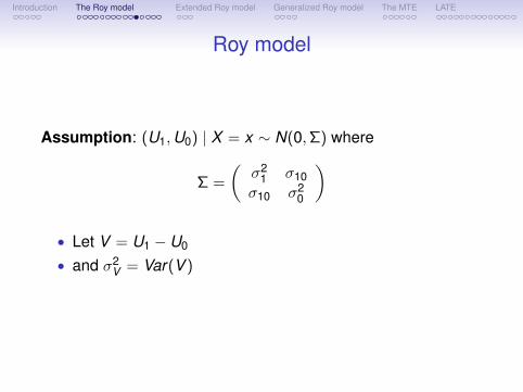
Assumption: (U1,U0) | X = x ∼ N(0,Σ) where
Σ =
(σ2
1 σ10σ10 σ2
0
)
• Let V = U1 − U0
• and σ2V = Var(V )

Introduction The Roy model Extended Roy model Generalized Roy model The MTE LATE
Roy model
Assumption: (U1,U0) | X = x ∼ N(0,Σ)
• Let z̃ = z∗/σV .• Then under this assumption,
E(Y | D = 1,X = x) = β′1x +σ2
1 − σ10
σVλ(−z̃)
E(Y | D = 0,X = x) = β′0x +σ2
0 − σ10
σVλ(z̃)
andPr(D = 1 | X = x) = Φ(z̃)
Introduction The Roy model Extended Roy model Generalized Roy model The MTE LATE
Roy model
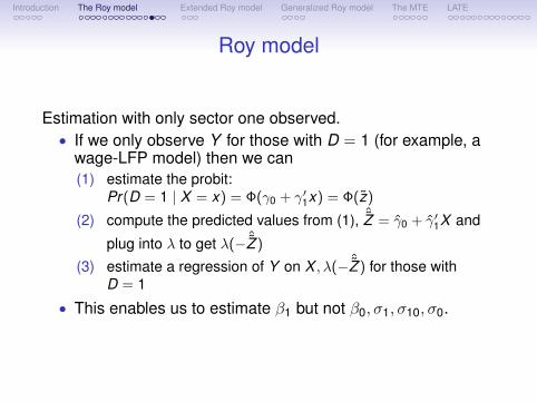
Estimation with only sector one observed.• If we only observe Y for those with D = 1 (for example, a
wage-LFP model) then we can(1) estimate the probit:
Pr(D = 1 | X = x) = Φ(γ0 + γ′1x) = Φ(z̃)
(2) compute the predicted values from (1), ˆ̃Z = γ̂0 + γ̂′1X and
plug into λ to get λ(− ˆ̃Z )
(3) estimate a regression of Y on X , λ(− ˆ̃Z ) for those withD = 1
• This enables us to estimate β1 but not β0, σ1, σ10, σ0.
Introduction The Roy model Extended Roy model Generalized Roy model The MTE LATE
Roy model
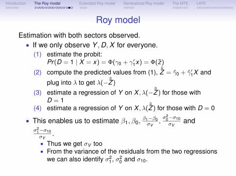
Estimation with both sectors observed.• If we only observe Y ,D,X for everyone.
(1) estimate the probit:Pr(D = 1 | X = x) = Φ(γ0 + γ′1x) = Φ(z̃)
(2) compute the predicted values from (1), ˆ̃Z = γ̂0 + γ̂′1X and
plug into λ to get λ(− ˆ̃Z )
(3) estimate a regression of Y on X , λ(− ˆ̃Z ) for those withD = 1
(4) estimate a regression of Y on X , λ( ˆ̃Z ) for those with D = 0
• This enables us to estimate β1, β0,β1−β0σV
,σ2
0−σ10σV
andσ2
1−σ10σV
.• Thus we get σV too• From the variance of the residuals from the two regressions
we can also identify σ21 , σ2
0 and σ10.

Introduction The Roy model Extended Roy model Generalized Roy model The MTE LATE
Roy model
Concerns:• If λ(−z̃) is approximately linear then we will have a serious
collinearity problem.• If U1,U0 is not normal then the model is misspecified and
identification is not transparent.• If there are variable costs the model is misspecified.

Introduction The Roy model Extended Roy model Generalized Roy model The MTE LATE
Roy model
• In the extended Roy model, Yd = µd + Ud for d = 0,1 but
D = 1(Y1 − Y0 ≥ γ′1X + γ′2Z )
• “‘Cost” of participation varies with X and also with othervariables Z .
• Then
E(Y | D = 1,X = x ,Z = z) = β′1x+ E(U1 | U1 − U0 ≥ −z∗,X = x)
E(Y | D = 0,X = x ,Z = z) = β′0x+ E(U0 | U1 − U0 < −z∗,X = x)
where z∗ = (β1 − β0)′x − γ′1x − γ′2z.
Introduction The Roy model Extended Roy model Generalized Roy model The MTE LATE
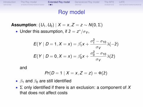
Roy model
Assumption: (U1,U0) | X = x ,Z = z ∼ N(0,Σ)
• Under this assumption, if z̃ = z∗/σV ,
E(Y | D = 1,X = x) = β′1x +σ2
1 − σ10
σVλ(−z̃)
E(Y | D = 0,X = x) = β′0x +σ2
0 − σ10
σVλ(z̃)
andPr(D = 1 | X = x ,Z = z) = Φ(z̃)
• β1 and β0 are still identified• Σ only identified if there is an exclusion: a component of X
that does not affect costs

Introduction The Roy model Extended Roy model Generalized Roy model The MTE LATE
Roy model
What do we need/want to identify?• The ATE is
E(Y1 − Y0) = (β1 − β0)E(X )
• The distribution of gains:
Y1 − Y0 | X = x ∼ N((β1 − β0)′x , σ2V )
• various other counterfactuals• need Σ to go beyond mean treatment effects

Introduction The Roy model Extended Roy model Generalized Roy model The MTE LATE
Roy model
• In the generalized Roy model, Yd = µd + Ud for d = 0,1but
D = 1(γ′1X + γ′2Z ≥ V )
• V includes an unobservable component of cost• Then
E(Y | D = 1,X = x ,Z = z) = β′1x+ E(U1 | V ≤ z∗,X = x)
E(Y | D = 0,X = x ,Z = z) = β′0x+ E(U0 | V > z∗,X = x)
where z∗ = γ′1x + γ′2z.

Introduction The Roy model Extended Roy model Generalized Roy model The MTE LATE
Roy model
Assumption: (U1,U0,V ) | X = x ,Z = z ∼ N(0,Σ)
• Under this assumption,• β1 and β0 are identified• σV is identified under the exclusion restriction• but Var(U1 − U0) 6= σ2
V (key ingredient needed fordistribution of Y1 − Y0) is not identified

Introduction The Roy model Extended Roy model Generalized Roy model The MTE LATE
Generalized roy model without normality
Assumption: (U1,U0,V ) ⊥⊥ X ,Z andlimz→∞ Pr(D = 1 | X = x ,Z = z) = 1• The first assumption is essentially the same one used by
Imbens and Angrist (1994)• The second assumption is called “identification at infinity”

Introduction The Roy model Extended Roy model Generalized Roy model The MTE LATE
Roy model without normality
• Under these assumptions• Let P(x , z) = Pr(D = 1 | X = x ,Z = z)• E(Y | D = 1,X = x ,Z = z) = β′1x + K1(P(x , z))• and limz→∞ E(Y | D = 1,X = x ,Z = z) = β′1x• selection on unobservables goes away in the limit• Using the same argument for D = 0, we can identify
ATE(x) = (β1 − β0)′x• We’ve traded normality for identification at infinity.

Introduction The Roy model Extended Roy model Generalized Roy model The MTE LATE
Some preliminaries
• Let D = 1(γ′1X + γ′2Z ≥ V ) and assume that(U1,U0,V ) ⊥⊥ (X ,Z )
• Let UD = FV (V ) where V has distribution function FV (·).• Then D = 1(P(X ,Z ) ≥ UD) where
P(X ,Z ) = FV (γ′1X + γ′2Z ) is the propensity score andUD ∼ Uniform(0,1).
Introduction The Roy model Extended Roy model Generalized Roy model The MTE LATE
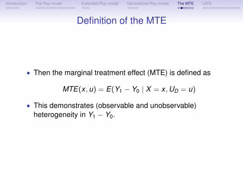
Definition of the MTE
• Then the marginal treatment effect (MTE) is defined as
MTE(x ,u) = E(Y1 − Y0 | X = x ,UD = u)
• This demonstrates (observable and unobservable)heterogeneity in Y1 − Y0.

Introduction The Roy model Extended Roy model Generalized Roy model The MTE LATE
Definition of the MTE
• MTE(x ,u) can be interpreted as the effect of participationfor those individuals who would be indifferent if weassigned them a new value of P = P(x , z) equal to u.• Someone with a large value of u (close to 1) will participate
only if P is quite large; this person will be indifferent if P isequal to u. These are the “high unobservable cost”individuals.
• Someone with a small value of u (close to 0) will participateeven if P is quite small; this person will be indifferent if P isequal to u. These are the “low unobservable cost”individuals.

Introduction The Roy model Extended Roy model Generalized Roy model The MTE LATE
Identification of the MTE
• The identifying equation:
∂E(Y | X = x ,P(X ,Z ) = p)
∂p= MTE(x ,p)
• This only works if Z is continuous.• The effect for the “high unobserved cost” individuals is
identified by the effect of a marginal increase inparticipation probability on Y at a high participation rate.

Introduction The Roy model Extended Roy model Generalized Roy model The MTE LATE
Other treatment parameters and methods
• ATE(x) =∫ 1
0 MTE(x ,u)du
• TT (x) =∫ 1
0 MTE(x ,u)ωTT (x ,u)du where ωTT (x ,u)disproportionately weights smaller values of u
• OLS and IV can also be written as weighted averages ofMTE(x ,u).

Introduction The Roy model Extended Roy model Generalized Roy model The MTE LATE
Other treatment parameters and methods
• Consider the IV estimand ∆IV (x) = Cov(J(Z ),Y |X=x)Cov(J(Z ),D|X=x)
• The weight here is
ωIV (x ,u) =E(J − E(J) | X = x ,P ≥ u)Pr(P ≥ u | X = x)
Cov(J,P | X = x)
• This and many interesting implications are discussed inHeckman, Vytlacil, and Urzua (2006).

Introduction The Roy model Extended Roy model Generalized Roy model The MTE LATE
LATE
• This is a limiting version of Imbens and Angrist’s LATEformulation.
• Ig nore X and let Dz denote the value of D when Z is fixedat z.
(i.e., Dz = 1(γ′2z ≥ V ))• Imbens and Angrist consider a binary Z and show that
E(Y | Z = 1)− E(Y | Z = 0)
E(D | Z = 1)− E(D | Z = 0)= E(Y1 − Y0 | D1 > D0)
• Thus, IV (lhs) identified the local average treatment effect(LATE, rhs), which is the average effect for those inducedto “participate” by Z . This population is sometimes calledthe “compliers”.

Introduction The Roy model Extended Roy model Generalized Roy model The MTE LATE
LATE
• This is a limiting version of Imbens and Angrist’s LATEformulation.
• Ig nore X and let Dz denote the value of D when Z is fixedat z. (i.e., Dz = 1(γ′2z ≥ V ))
• Imbens and Angrist consider a binary Z and show that
E(Y | Z = 1)− E(Y | Z = 0)
E(D | Z = 1)− E(D | Z = 0)= E(Y1 − Y0 | D1 > D0)
• Thus, IV (lhs) identified the local average treatment effect(LATE, rhs), which is the average effect for those inducedto “participate” by Z . This population is sometimes calledthe “compliers”.

Introduction The Roy model Extended Roy model Generalized Roy model The MTE LATE
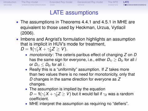
LATE assumptions• The assumptions in Theorems 4.4.1 and 4.5.1 in MHE are
equivalent to those used by Heckman, Urzua, Vytlacil(2006).
• Imbens and Angrist’s formulation highlights an assumptionthat is implicit in HUV’s mode for treatment,D = 1(γ′1X + γ′2Z ≥ V ).• monotonicity : The ceteris paribus effect of changing Z on D
has the same sign for everyone, i.e., either D1i ≥ D0i for all ior D1i ≤ D0i for all i .
• Really this is a “uniformity” assumption. If Z takes morethan two values there is no need for monotonicity, only thatD changes in the same direction for everyone as Zchanges.
• The assumption is implied by the equationD = 1(γ′1X + γ′2Z ≥ V ) but it would fail if γ2 was a randomcoefficient.
• MHE interpret the assumption as requiring no “defiers”.
Introduction The Roy model Extended Roy model Generalized Roy model The MTE LATE
LATE assumptions
• The independence assumption when there are covariates.• Really only need (U1,U0,V ) ⊥⊥ Z | X .• Estimation of MTE is simplified under the stronger
assumption that (U1,U0,V ) ⊥⊥ Z | X .• See the discussion in Carneiro, Heckman, Vytlacil (2011).

Introduction The Roy model Extended Roy model Generalized Roy model The MTE LATE
More on LATE
• When Z is continuous, we can estimate the MTE andvarious weighted averages of the MTE.
• The LATE framework is useful in understanding what weare able to learn when Z is discrete.• Cases where LATE = TT or LATE = TUT• Characterizing compliers.• LATE with covariates

Introduction The Roy model Extended Roy model Generalized Roy model The MTE LATE
Special cases
• The TT can be written as a weighted average of LATE andthe average effect for the always-takers.
• In some cases, D must be equal to 0 when Z = 0.• The Bloom example – Z is a random assignment and D a
treatment and there is one-way noncompliance.• One-way noncompliance means that some with Z = 1
choose D = 0 (refuse treatment) but no one with Z = 0 canhave D = 1.
• In these cases, IV estimates TT.
Introduction The Roy model Extended Roy model Generalized Roy model The MTE LATE
Special cases
• The TUT can be written as a weighted average of LATEand the average effect for the never-takers.
• In some cases, D must be equal to 1 when Z = 1.• Suppose D indicates having a third child (as opposed to
only 2) and Z indicates whether the second birth was amultiple birth.
• Then if Z = 1 we must have D = 1.• There are no “never-takers”.
• In these cases, IV estimates TUT.

Introduction The Roy model Extended Roy model Generalized Roy model The MTE LATE
Compliers
• A few results:• Pr(D1 > D0) = E(D | Z = 1)− E(D | Z = 0)• for any W such that (D1,D0) is independent of Z
conditional on W , E(W | D1 > D0) = E(κW )E(κ) where
κ = 1− D(1− Z )
1− Pr(Z = 1 |W )− (1− D)Z
Pr(Z = 1 |W )
• and, more generally, fW |D1>D0 (w) is equal to
E(D | Z = 1,W = w)− E(D | Z = 0,W = w)
E(D | Z = 1)− E(D | Z = 0)fW (w)
Introduction The Roy model Extended Roy model Generalized Roy model The MTE LATE
LATE with covariates• The LATE story gets quite a bit more complicated with
covariates.• Let λ(x) = E(Y1 − Y0 | D1 > D0,X = x) denote the LATE
conditional on X .• We could estimate these directly using the Wald formula
conditional on X .
• If we do 2SLS where the first stage is fully saturated andthe second stage is saturated in X we get a weightedaverage of the λ(x).• The weights are larger for values of x such that
Var(E(D | X = x ,Z ) | X = x) is larger.• if Pr(Z = 1 | X ) is a linear function of X then 2SLS gives
the minimum MSE approximation to E(Y | D,X ,D1 > D0).• This is useful because E(Y | D = 1,X ,D1 > D0)− E(Y |
D = 0,X ,D1 > D0) = λ(X ).• Abadie (2003) proposes a way to estimate this same
minimum MSE approximation when Pr(Z = 1 | X ) is notlinear.

Introduction The Roy model Extended Roy model Generalized Roy model The MTE LATE
LATE with covariates• The LATE story gets quite a bit more complicated with
covariates.• Let λ(x) = E(Y1 − Y0 | D1 > D0,X = x) denote the LATE
conditional on X .• We could estimate these directly using the Wald formula
conditional on X .• If we do 2SLS where the first stage is fully saturated and
the second stage is saturated in X we get a weightedaverage of the λ(x).• The weights are larger for values of x such that
Var(E(D | X = x ,Z ) | X = x) is larger.
• if Pr(Z = 1 | X ) is a linear function of X then 2SLS givesthe minimum MSE approximation to E(Y | D,X ,D1 > D0).• This is useful because E(Y | D = 1,X ,D1 > D0)− E(Y |
D = 0,X ,D1 > D0) = λ(X ).• Abadie (2003) proposes a way to estimate this same
minimum MSE approximation when Pr(Z = 1 | X ) is notlinear.
Introduction The Roy model Extended Roy model Generalized Roy model The MTE LATE
LATE with covariates• The LATE story gets quite a bit more complicated with
covariates.• Let λ(x) = E(Y1 − Y0 | D1 > D0,X = x) denote the LATE
conditional on X .• We could estimate these directly using the Wald formula
conditional on X .• If we do 2SLS where the first stage is fully saturated and
the second stage is saturated in X we get a weightedaverage of the λ(x).• The weights are larger for values of x such that
Var(E(D | X = x ,Z ) | X = x) is larger.• if Pr(Z = 1 | X ) is a linear function of X then 2SLS gives
the minimum MSE approximation to E(Y | D,X ,D1 > D0).• This is useful because E(Y | D = 1,X ,D1 > D0)− E(Y |
D = 0,X ,D1 > D0) = λ(X ).• Abadie (2003) proposes a way to estimate this same
minimum MSE approximation when Pr(Z = 1 | X ) is notlinear.

Introduction The Roy model Extended Roy model Generalized Roy model The MTE LATE
An example
Carneiro, Heckman, Vytlacil (2011)• use data from the NLSY• Y is log wage in 1991 (ages 28-34), D represents college
attendance, X a vector of controls• vector Z : (i) distance to college, (ii) local wage, (iii) local
unemployment, (iv) average local public tuition

Introduction The Roy model Extended Roy model Generalized Roy model The MTE LATE
An example
Review of IV Roy Model Generalized Roy Model MTE
MTE2771cARnEiRO Et Al.: EStimAting mARginAl REtuRnS tO EducAtiOnVOl. 101 nO. 6
mean values in the sample. As above, we annualize the MTE. Our estimates show that, in agreement with the normal model, E( u 1 − u 0 | u S = u S ) is declining in u S , i.e., students with high values of u S have lower returns than those with low values of u S .
Even though the semiparametric estimate of the MTE has larger standard errors than the estimate based on the normal model, we still reject the hypothesis that its slope is zero. We have already discussed the rejection of the hypothesis that MTE is constant in u S , based on the test results reported in Table 4, panel A. But we can also directly test whether the semiparametric MTE is constant in u S or not. We evaluate the MTE at 26 points, equally spaced between 0 and 1 (with intervals of 0.04). We construct pairs of nonoverlapping adjacent intervals (0–0.04, 0.08–0.12, 0.16–0.20, 0.24–0.28, …), and we take the mean of the MTE for each pair. These are LATEs defined over different sections of the MTE. We compare adjacent LATEs. Table 4, panel B, reports the outcome of these comparisons. For example, the first column reports that
E ( Y 1 − Y 0 | X = _ x , 0 ≤ u S ≤ 0.04)
− E ( Y 1 − Y 0 | X = _ x , 0.08 ≤ u S ≤ 0.12) = 0.0689.
0 0.1 0.2 0.3 0.4 0.5 0.6 0.7 0.8 0.9 1−0.6
−0.4
−0.2
0
0.2
0.4
0.6
0.8
US
MT
E
Figure 4. E( Y 1 − Y 0 | X, u S ) with 90 Percent Confidence Interval— Locally Quadratic Regression Estimates
notes: To estimate the function plotted here, we first use a partially linear regression of log wages on polynomials in X, interactions of polynomials in X and P, and K(P), a locally quadratic function of P (where P is the predicted probability of attending college), with a bandwidth of 0.32; X includes experience, current average earnings in the county of residence, current average unemployment in the state of residence, AFQT, mother’s education, number of siblings, urban residence at 14, permanent local earnings in the county of residence at 17, permanent unemployment in the state of residence at 17, and cohort dummies. The figure is generated by evaluating by the derivative of (9) at the average value of X. Ninety percent standard error bands are obtained using the bootstrap (250 replications).
Economics 379 George Washington University
Lecture 4

Introduction The Roy model Extended Roy model Generalized Roy model The MTE LATE
• Estimating the MTE - normal model• Option 1. Estimate using MLE.• Option 2. Two stage estimation:
• Probit to estimate P(Zi ) (to simplify, define Zi to include Xi
and instrument(s))• Regress Y on Xi and λ̂1i = −φ(Φ−1(P̂(Zi )))
P̂(Zi )for Di = 1
• Regress Y on Xi and λ̂0i = φ(Φ−1(P̂(Zi )))
1−P̂(Zi )for Di = 0
• Then
MTE(x , u) = x ′(β̂1 − β̂0) + (ρ̂1 − ρ̂0)Φ−1(u)

Introduction The Roy model Extended Roy model Generalized Roy model The MTE LATE
• Estimating the MTE – semiparametric model• The outcome equation can be written (see II.B in Carneiro
et al. (2011)) as
E(Y | X = x ,P(Z ) = p) = x ′δ0 + px ′(δ1 − δ0) + K (p)
• There are several ways to estimate this – perhaps thesimplest is a series/spline/sieve estimator.• Estimate P(Zi ) (logit).• Choose a set of basis functions (polynomials) and an order,
K .• Run the regression:
Yi = X ′i δ0 + P̂(Zi )X ′i (δ1 − δ0) + γ1P̂(Zi ) + . . .+ γK P̂(Zi )K + ηi
• An important sacrifice here is that MTE(x ,u) is onlyidentified for u in the support of P. (Recall identification at∞)

Introduction The Roy model Extended Roy model Generalized Roy model The MTE LATE
• Consider policies that affect P(Z ) but not Y1,Y0,V .• Propensity score P∗ under new policy.• It can be shown that the effect of shifting to this new policy
is given by∫ 1
0MTE(x ,u)
[FP∗|X=x (u)− FP|X=x (u)
E(P∗ | X = x)− E(P | X = x)
]du
• This will still require large support for P(Z ).• define a continuum of policies• consider marginal change from baseline
Introduction The Roy model Extended Roy model Generalized Roy model The MTE LATE
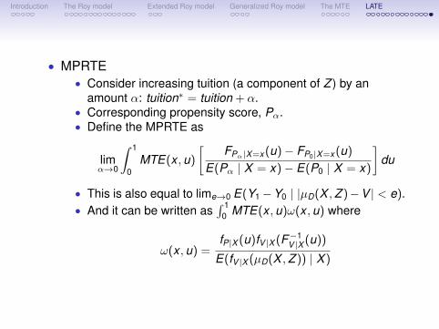
• MPRTE• Consider increasing tuition (a component of Z ) by an
amount α: tuition∗ = tuition + α.• Corresponding propensity score, Pα.• Define the MPRTE as
limα→0
∫ 1
0MTE(x ,u)
[FPα|X=x (u)− FP0|X=x (u)
E(Pα | X = x)− E(P0 | X = x)
]du
• This is also equal to lime→0 E(Y1−Y0 | |µD(X ,Z )−V | < e).• And it can be written as
∫ 10 MTE(x ,u)ω(x ,u) where
ω(x ,u) =fP|X (u)fV |X (F−1
V |X (u))
E(fV |X (µD(X ,Z )) | X )