Lecture 9 — Nonlinear Control Design

I Exact-linearizationI Lyapunov-based design

I Lab 2I Adaptive control

I Sliding modes control

Literature: [Khalil, ch.s 13, 14.1,14.2] and [Glad-Ljung,ch.17]

Course Outline

Lecture 1-3 Modelling and basic phenomena(linearization, phase plane, limit cycles)

Lecture 4-6 Analysis methods(Lyapunov, circle criterion, describing functions)

Lecture 7-8 Common nonlinearities(Saturation, friction, backlash, quantization)

Lecture 9-13 Design methods(Lyapunov methods, optimal control)

Lecture 14 Summary

Exact Feedback Linearization

Idea:Find state feedback u = u(x, v) so that the nonlinear system

x = f(x) + g(x)u

turns into the linear system

x = Ax+Bv

and then apply linear control design method.

Exact linearization: example [one-link robot]

l

tth

m

m`2θ + dθ +m`g cos θ = u

where d is the viscous damping.The control u = τ is the applied torqueDesign state feedback controller u = u(x) with x = (θ, θ)T

Introduce new control variable v and let

u = m`2v + dθ +m`g cos θ

Thenθ = v

Choose e.g. a PD-controller

v = v(θ, θ) = kp(θref − θ)− kdθ

This gives the closed-loop system:

θ + kdθ + kpθ = kpθref

Hence, u = m`2[kp(θ − θref)− kdθ] + dθ +m`g cos θ

Multi-link robot (n-joints)

x

y

z

u

phi

theta

General form

M(θ)θ + C(θ, θ)θ +G(θ) = u, θ ∈ Rn

Called fully actuated if n indep. actuators,

M n× n inertia matrix, M =MT > 0

Cθ n× 1 vector of centrifugal and Coriolis forcesG n× 1 vector of gravitation terms

Computed torque

The computed torque(also known as ”Exact linearization”, ”dynamic inversion” , etc. )

u =M(θ)v + C(θ, θ)θ +G(θ)

v = Kp(θref − θ)−Kdθ,(1)

gives closed-loop system

θ +Kdθ +Kpθ = KpθRef

The matrices Kd and Kp can be chosen diagonal (no cross-terms)and then this decouples into n independent second-order equations.

Lyapunov-Based Control Design Methods

x = f(x, u)

I Select Lyapunov function V (x) for stability verification

I Find state feedback u = u(x) that makes V decreasing

I Method depends on structure of f

Examples are energy shaping as in Lab 2 and, e.g., Back-steppingcontrol design, which require certain f discussed later.

Lab 2 : Energy shaping for swing-up control

[movie]

Use Lyapunov-based design for swing-up control.

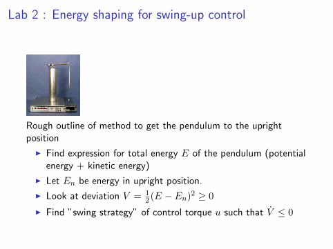
Lab 2 : Energy shaping for swing-up control

Rough outline of method to get the pendulum to the uprightposition

I Find expression for total energy E of the pendulum (potentialenergy + kinetic energy)

I Let En be energy in upright position.

I Look at deviation V = 12(E − En)

2 ≥ 0

I Find ”swing strategy” of control torque u such that V ≤ 0

Example of Lyapunov-based design

Consider the nonlinear system

x1 = −3x1 + 2x1x22 + u (2)

x2 = −x32 − x2,

Find a nonlinear feedback control law which makes the originglobally asymptotically stable.We try the standard Lyapunov function candidate

V (x1, x2) =1

2

(x21 + x22

),

which is radially unbounded, V (0, 0) = 0, andV (x1, x2) > 0 ∀(x1, x2) 6= (0, 0).

Example - cont’d

V = x1x1 + x2x2 = (−3x1 + 2x1x22 + u)x1 + (−x32 − x2)x2

= −3x21 − x22+ux1+2x21x22 − x42

We would like to have

V < 0 ∀(x1, x2) 6= (0, 0)

Inserting the control law, u = −2x1x22, we get

V = −3x21−x22−2x21x22 + 2x21x22︸ ︷︷ ︸

=0

−x42 = −3x21−x22−x42 < 0, ∀x 6= 0

Consider the system

x1 = x32

x2 = u(3)

Find a globally asymptotically stabilizing control law u = u(x).Attempt 1: Try the standard Lyapunov function candidate

V (x1, x2) =1

2

(x21 + x22

),

which is radially unbounded, V (0, 0) = 0, andV (x1, x2) > 0 ∀(x1, x2) 6= (0, 0).

V = x1x1 + x2x2 = x32 · x1 + u · x2 = x2 (x22x1 + u)︸ ︷︷ ︸−x2

= −x22 ≤ 0

where we choseu = −x2 − x22x1

However V = 0 as soon as x2 = 0 (Note: x1 could be anything).According to LaSalle’s theorem the setE = {x|V = 0} = {(x1, 0)} ∀x1What is the largest invariant subset M ⊆ E?Plugging in the control law u = −x2 − x22x1, we get

x1 = x32

x2 = −x2 − x22x1(4)

Observe that if we start anywhere on the line {(x1, 0)} we will stayin the same point as both x1 = 0 and x2 = 0, thus M=E and wewill not converge to the origin, but get stuck on the line x2 = 0.

Draw phase-plot with e.g., pplane and study the behaviour.

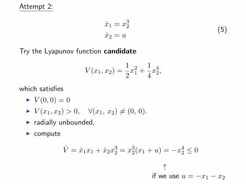
Attempt 2:

x1 = x32

x2 = u(5)

Try the Lyapunov function candidate

V (x1, x2) =1

2x21 +

1

4x42,

which satisfies

I V (0, 0) = 0

I V (x1, x2) > 0, ∀(x1, x2) 6= (0, 0).

I radially unbounded,

I compute

V = x1x1 + x2x32 = x32(x1 + u) = −x42 ≤ 0

↑if we use u = −x1 − x2

Withu = −x1 − x2

we get the dynamics

x1 = x32

x2 = −x1 − x2(6)

V = 0 if x2 = 0, thus

E = {x|V = 0} = {(x1, 0)∀x1}

However, now the only possibility to stay on x2 = 0 is if x1 = 0, (else x2 6= 0 and we will leave the line x2 = 0).Thus, the largest invariant set

M = (0, 0)

According to the Invariant Set Theorem (LaSalle) all solutions willend up in M and so the origin is GAS.Draw phase-plot with e.g., pplane and study the behaviour.

Adaptive Noise Cancellation Revisited

u

g1

g2

x

xh

xt

+

-

x+ ax = bu

˙x+ ax = bu

Introduce x = x− x, a = a− a, b = b− b.Want to design adaptation law so that x→ 0

Let us try the Lyapunov function

V =1

2(x2 + γaa

2 + γbb2)

V = x ˙x+ γaa ˙a+ γbb˙b =

= x(−ax− ax+ bu) + γaa ˙a+ γbb˙b = −ax2

where the last equality follows if we choose

˙a = − ˙a =1

γaxx

˙b = − ˙b = − 1

γbxu

Invariant set: x = 0.This proves that x→ 0.(The parameters a and b do not necessarily converge: u ≡ 0.)

A Control Design Idea, and a Problem

Assume V (x) = xTPx, P > 0, represents the energy of

x = Ax+Bu, u ∈ [−1, 1]

Idea: Choose u such that V decays as fast as possible

V = xT (ATP +AP )x+ 2BTPx · uu = −sgn(BTPx)

The following situation might then occur (“system is notLipschitz”)

f+

f-

s

Sliding Modes

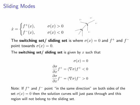
x =

{f+(x), σ(x) > 0

f−(x), σ(x) < 0

f+

f-

s-

s+

The switching set/ sliding set is where σ(x) = 0 and f+ and f−

point towards σ(x) = 0.

The switching set/ sliding set is given by x such that

σ(x) = 0

∂σ

∂xf+ = (∇σ)f+ < 0

∂σ

∂xf− = (∇σ)f− > 0

Note: If f+ and f− point “in the same direction” on both sides of the

set σ(x) = 0 then the solution curves will just pass through and this

region will not belong to the sliding set.

Sliding Mode

If f+ and f− both points towards σ(x) = 0, what will happenthen?

The sliding dynamics are x = αf+ + (1− α)f−, where α is

obtained fromdσ

dt=∂σ

∂x· x = 0 on {σ(x) = 0}.

f+

f-

s-

s+

More precisely, find α such that the components of f+ and f−

perpendicular to the switching surface cancel: αf+⊥ + (1− α)f−⊥ = 0 The

resulting dynamics is then the sum of the corresponding components

along the surface.

4 minute exercise

x =

[0 −11 −1

]x+

[11

]u = Ax+Bu

u = −sgnσ(x) = −sgnx2 = −sgn(Cx)

which means that

x =

{Ax−B, x2 > 0

Ax+B, x2 < 0

Determine the switching set and the sliding dynamics.

4 minute exercise — Solution

x1 = −x2 + u = −x2 − sgn(x2)

x2 = x1 − x2 + u = x1 − x2 − sgn(x2)

f+ =

[−x2 − 1

x1 − x2 − 1

]f− =

[−x2 + 1

x1 − x2 + 1

]

σ(x) = x2 = 0 ⇒ x2 = 0

∂σ

∂xf+ =

[0 1

]f+ = x1 − x2 − 1 < 0 ⇒ x1 < 1

∂σ

∂xf− =

[0 1

]f− = x1 − x2 + 1 > 0 ⇒ x1 > −1

We will thus have a sliding set for {−1 < x1 < 1, x2 = 0}

The normal projections of (f+, f−) to σ(x) = x2 = 0 are

f+⊥ =

[0

x1 − x2 − 1

]f−⊥ =

[0

x1 − x2 + 1

]Find α ∈ [0, 1] such that αf+⊥ + (1− α)f−⊥ = 0 on {x2 = 0}

α(x1 − x2 − 1) + (1− α)(x1 − x2 + 1) = 0

⇒

α =x1 + 1

2as x2 = 0

Note: α ∈ [0, 1]⇒ x1 ∈ [−1, 1]

The sliding dynamics are the given by

x = αf+ + (1− α)f−[x1x2

]= α

[−x2 − 1

x1 − x2 − 1

]+ (1− α)

[−x2 + 1

x1 − x2 + 1

]=

[−2α− x2 − 1

0

]=

[−x10

]where we inserted x2 = 0 and α = x1+1

2

We see that on the sliding set {−1 < x < 1, x2 = 0} we have

x1 = −x1x2 = 0

For any initial condition starting on the sliding set, there will beexponential convergence to x1 = x2 = 0.

For small x2 we havex2(t) ≈ x1 − 1,

dx2dx1

=dx2/dt

dx1/dt≈ 1− x1 x2 > 0

x2(t) ≈ x1 + 1,dx2dx1

=dx2/dt

dx1/dt≈ 1 + x1 x2 < 0

This implies the following behavior

>

=

<

−1 +1

Sliding Mode Dynamics

The dynamics along the sliding set in σ(x) = 0 can also beobtained by finding u = ueq ∈ [−1, 1] such that σ(x) = 0.ueq is called the equivalent control.

Example (cont’d)

Finding u = ueq such that σ(x) = x2 = 0 gives

0 = x2 = x1 − x2︸︷︷︸=0

+ueq = x1 + ueq

Insert ueq = −x1 in the equation for x1:

x1 = − x2︸︷︷︸=0

+ueq = −x1

gives the dynamics on the sliding set (where x2 = 0)

Remember: ueq ∈ [−1, 1] so can only satisfy ueq = −x1 on the interval

x1 ∈ [−1, 1]!

Equivalent Control

Assume

x = f(x) + g(x)u

u = −sgnσ(x)

has a sliding set on σ(x) = 0. Then, for x(t) staying on the slidingset we should have

0 = σ(x) =∂σ

∂x· dxdt

=∂σ

∂x

(f(x) + g(x)u

)The equivalent control is thus given by solving

ueq = −(∂σ

∂xg(x)

)−1∂σ∂xf(x)

for all those x such that σ(x) = 0 and ∂σ∂xg(x) 6= 0.

Equivalent Control for Linear System

x = Ax+Bu

u = −sgnσ(x) = −sgn(Cx)

Assume CB invertible. The sliding set lies in σ(x) = Cx = 0.

0 = σ(x) =dσ

dx

(f(x) + g(x)u

)= C

(Ax+Bueq

)gives CBueq = −CAx.Example (cont’d) For the previous system

ueq = −(CB)−1CAx = −(x1 − x2)/1 = −x1,

because σ(x) = x2 = 0. Same result as above.

More on the Sliding Dynamics

If CB > 0 then the dynamics along a sliding set in Cx = 0 is

x = Ax+Bueq =

(I − (CB)−1BC

)Ax,

One can show that the eigenvalues of (I − (CB)−1BC)A equalsthe zeros of G(s) = C(sI −A)−1B. (exercise for PhD students)

Design of Sliding Mode Controller

Idea: Design a control law that forces the state to σ(x) = 0.Choose σ(x) such that the sliding mode tends to the origin.Assume system has form

d

dt

x1x2...xn

=

f1(x) + g1(x)u

x1...

xn−1

= f(x) + g(x)u

Choose control law

u = −pT f(x)

pT g(x)− µ

pT g(x)sgnσ(x),

where µ > 0 is a design parameter, σ(x) = pTx, andpT =

[p1 . . . pn

]represents a stable polynomial.

Sliding Mode Control gives Closed-Loop Stability

Consider V(x) = σ2(x)/2 with σ(x) = pTx. Then,

V = σ(x)σ(x) = xT p(pT f(x) + pT g(x)u

)With the chosen control law, we get

V = −µσ(x)sgnσ(x) ≤ 0

so σ(x)→ 0 as t→ +∞. In fact, one can prove that this occursin finite time.

0 = σ(x) = p1x1 + · · ·+ pn−1xn−1 + pnxn

= p1x(n−1)n + · · ·+ pn−1x

(1)n + pnx

(0)n

where x(k) denote time derivative. P stable gives that x(t)→ 0.

Note: V by itself does not guarantee stability. It only guarantees

convergence to the line {σ(x) = 0} = {pTx = 0}.

Time to Switch

Consider an initial point x such that σ0 = σ(x) > 0. Then

σ(x)σ(x) = −µσ(x)sgnσ(x)

soσ(x) = −µ

Hence, the time to the first switch is

ts =σ0µ<∞

Note that ts → 0 as µ→∞.

Example—Sliding Mode Controller

Design state-feedback controller for

x =

[1 01 0

]x+

[10

]u

y =[0 1

]x

Choose p1s+ p2 = s+ 1 so that σ(x) = x1 + x2. The controller isgiven by

u = −pTAx

pTB− µ

pTBsgnσ(x)

= −2x1 − µsgn(x1 + x2)

Phase Portrait

Simulation with µ = 0.5. Note the sliding set is in σ(x) = x1 + x2.

−2 −1 0 1 2

−1

0

1

x2

x1

s

Time Plots

Initial conditionx(0) =

[1.5 0

]T.

Simulation agrees well withtime to switch

ts =σ0µ

= 3

and sliding dynamics

y = −y

x2

x1

u

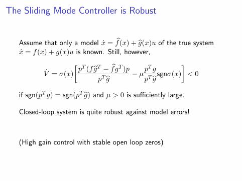
The Sliding Mode Controller is Robust

Assume that only a model x = f(x) + g(x)u of the true systemx = f(x) + g(x)u is known. Still, however,

V = σ(x)

[pT (fgT − fgT )p

pT g− µp

T g

pT gsgnσ(x)

]< 0

if sgn(pT g) = sgn(pT g) and µ > 0 is sufficiently large.

Closed-loop system is quite robust against model errors!

(High gain control with stable open loop zeros)

ImplementationA relay with hysteresis or a smooth (e.g. linear) region is oftenused in practice.Choice of hysteresis or smoothing parameter can be critical forperformanceMore complicated structures with several relays possible. Harder todesign and analyze.

Next Lectures

I L10–L12: Optimal control methods

I L13: Other synthesis methods

I L14: Course summary

Next Lecture

I Optimal control

Read chapter 18 in [Glad & Ljung] for preparation.