lecture about gene prediction, algorithms for -
TRANSCRIPT

Genvorhersage
Dr. Mario Stanke
Lernziele / Study Aims
Introduction toGene-Finding-ProblemWhat Do Genes Look Like?
Statistical Features ofGenes
Gene Finding ThroughExon-ChainingThe One-DimensionalChaining Problem
Exon-Chaining Algorithm
Gene Finding withHMMsGeneralized HMMs
Model Design
Training
Pair Hidden MarkovModelsDefinitions
Application: ComparativeGene Prediction
1.1
Kapitel 1GenvorhersageVorlesung Algorithmen der Bioinformatik II vom 27 und 29.April 2010
Dr. Mario StankeInstitut für Mikrobiologie und Genetik
Universität Göttingen

Genvorhersage
Dr. Mario Stanke
Lernziele / Study Aims
Introduction toGene-Finding-ProblemWhat Do Genes Look Like?
Statistical Features ofGenes
Gene Finding ThroughExon-ChainingThe One-DimensionalChaining Problem
Exon-Chaining Algorithm
Gene Finding withHMMsGeneralized HMMs
Model Design
Training
Pair Hidden MarkovModelsDefinitions
Application: ComparativeGene Prediction
1.2
These Slides Available At:
http://gobics.de/mario/AbiII
Genvorhersage
Dr. Mario Stanke
Lernziele / Study Aims
Introduction toGene-Finding-ProblemWhat Do Genes Look Like?
Statistical Features ofGenes
Gene Finding ThroughExon-ChainingThe One-DimensionalChaining Problem
Exon-Chaining Algorithm
Gene Finding withHMMsGeneralized HMMs
Model Design
Training
Pair Hidden MarkovModelsDefinitions
Application: ComparativeGene Prediction
1.3
The study aims of this week.
1 understand the problem setting of gene finding2 learn about algorithmic solutions: exon chaining, GHMMs3 learn about pair HMMs
(used both for gene finding and alignments)
Genvorhersage
Dr. Mario Stanke
Lernziele / Study Aims
Introduction toGene-Finding-ProblemWhat Do Genes Look Like?
Statistical Features ofGenes
Gene Finding ThroughExon-ChainingThe One-DimensionalChaining Problem
Exon-Chaining Algorithm
Gene Finding withHMMsGeneralized HMMs
Model Design
Training
Pair Hidden MarkovModelsDefinitions
Application: ComparativeGene Prediction
1.4
Overview
1 Introduction to Gene-Finding-ProblemWhat Do Genes Look Like?Statistical Features of Genes
2 Gene Finding Through Exon-ChainingThe One-Dimensional Chaining ProblemExon-Chaining Algorithm
3 Gene Finding with HMMsGeneralized HMMsModel DesignTraining
4 Pair Hidden Markov ModelsDefinitionsApplication: Comparative Gene Prediction
Genvorhersage
Dr. Mario Stanke
Lernziele / Study Aims
Introduction toGene-Finding-ProblemWhat Do Genes Look Like?
Statistical Features ofGenes
Gene Finding ThroughExon-ChainingThe One-DimensionalChaining Problem
Exon-Chaining Algorithm
Gene Finding withHMMsGeneralized HMMs
Model Design
Training
Pair Hidden MarkovModelsDefinitions
Application: ComparativeGene Prediction
1.5
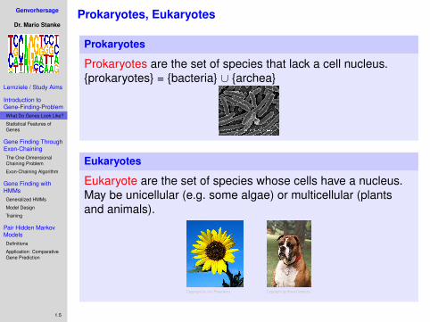
Prokaryotes, Eukaryotes
Prokaryotes
Prokaryotes are the set of species that lack a cell nucleus.{prokaryotes} = {bacteria} ∪ {archea}
Eukaryotes
Eukaryote are the set of species whose cells have a nucleus.May be unicellular (e.g. some algae) or multicellular (plantsand animals).
Copyright by Jim Pisarowicz Copyright by Broad Institute
Genvorhersage
Dr. Mario Stanke
Lernziele / Study Aims
Introduction toGene-Finding-ProblemWhat Do Genes Look Like?
Statistical Features ofGenes
Gene Finding ThroughExon-ChainingThe One-DimensionalChaining Problem
Exon-Chaining Algorithm
Gene Finding withHMMsGeneralized HMMs
Model Design
Training
Pair Hidden MarkovModelsDefinitions
Application: ComparativeGene Prediction
1.6
Prokaryotes, Eukaryotes
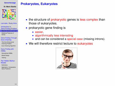
• the structure of prokaryotic genes is less complex thanthose of eukaryotes.
• prokaryotic gene finding is• easier,• algorithmically less interesting• and can be considered a special case (missing introns).
• We will therefore restrict lecture to eukaryotes
Genvorhersage
Dr. Mario Stanke
Lernziele / Study Aims
Introduction toGene-Finding-ProblemWhat Do Genes Look Like?
Statistical Features ofGenes
Gene Finding ThroughExon-ChainingThe One-DimensionalChaining Problem
Exon-Chaining Algorithm
Gene Finding withHMMsGeneralized HMMs
Model Design
Training
Pair Hidden MarkovModelsDefinitions
Application: ComparativeGene Prediction
1.6
Prokaryotes, Eukaryotes
• the structure of prokaryotic genes is less complex thanthose of eukaryotes.
• prokaryotic gene finding is• easier,• algorithmically less interesting• and can be considered a special case (missing introns).
• We will therefore restrict lecture to eukaryotes

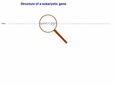
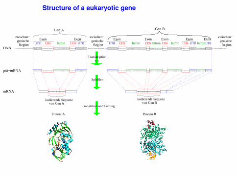
Structure of a eukaryotic gene
UTR = UnTranslated Region = part of mRNA that is not translatedCDS = CcoDing Sequence = part of mRNA (exon) that is translated
gene A
DNA
gene B
...actaatagacatctatttcgagtcaaggtgtaggcaatgtccttttttctagtcatggttggcaaacagtgggatcctgagagtcagataattgaattggctctgcctttaattatttgttcaagcaagcccctgtccctttaggtgggaatatgtatgagggaccatatttggggttctggtagctccacagggatgcggtgatgagcgctgaatttatgacgtactag...
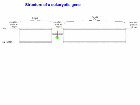
Structure of a eukaryotic gene
UTR = UnTranslated Region = part of mRNA that is not translatedCDS = CcoDing Sequence = part of mRNA (exon) that is translated
gene A
DNA
gene B
gaattggc...actaatagacatctatttcgagtcaaggtgtaggcaatgtccttttttctagtcatggttggcaaacagtg aattatttgttcaagcaagcccctgtccctttaggtgggaatatgtatgagggaccatatttggggttctggtagctccacagggatgcggtgatgagcgctgaatttatgacgtactag...

Structure of a eukaryotic gene
UTR = UnTranslated Region = part of mRNA that is not translatedCDS = CcoDing Sequence = part of mRNA (exon) that is translated
Region
zwischen−genische
Region
zwischen−genische
Region
zwischen−genische
Gen A
DNA
Gen B
...actaatagacatctatttcgagtcaaggtgtaggcaatgtccttttttctagtcatggttggcaaacagtgggatcctgagagtcagataattgaattggctctgcctttaattatttgttcaagcaagcccctgtccctttaggtgggaatatgtatgagggaccatatttggggttctggtagctccacagggatgcggtgatgagcgctgaatttatgacgtactag...
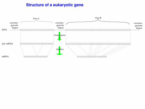
Structure of a eukaryotic gene
UTR = UnTranslated Region = part of mRNA that is not translatedCDS = CcoDing Sequence = part of mRNA (exon) that is translated
Region
zwischen−genische
Region
zwischen−genische
Region
zwischen−genische
Gen A
Transkription
DNA
prä−mRNA
Gen B
1:1
cgagucaagguguaggcaauguccuuuuuucuagucaugguuggcaaacagugggaucc
...actaatagacatctatttcgagtcaaggtgtaggcaatgtccttttttctagtcatggttggcaaacagtgggatcctgagagtcagataattgaattggctctgcctttaattatttgttcaagcaagcccctgtccctttaggtgggaatatgtatgagggaccatatttggggttctggtagctccacagggatgcggtgatgagcgctgaatttatgacgtactag...
gcucugccuuuaauuauuuguucaagcaagccccugucccuuuaggugggaauauguaugagggaccauauuugggguucugguagcuccacagggaugcggugaugagcgcugaa
Structure of a eukaryotic gene
UTR = UnTranslated Region = part of mRNA that is not translatedCDS = CcoDing Sequence = part of mRNA (exon) that is translated
Region
zwischen−genische
Region
zwischen−genische
Region
zwischen−genische
Gen A
Transcription
Spleißen
DNA
prä−mRNA
mRNA
Gen B
1:1
gcucugccuuuaauuauuugugguggacguagcuccacagggaugcgcugaacgagucaagguguaggcaaugucuuggcaaacagugggaucc
cgagucaagguguaggcaauguccuuuuuucuagucaugguuggcaaacagugggaucc
...actaatagacatctatttcgagtcaaggtgtaggcaatgtccttttttctagtcatggttggcaaacagtgggatcctgagagtcagataattgaattggctctgcctttaattatttgttcaagcaagcccctgtccctttaggtgggaatatgtatgagggaccatatttggggttctggtagctccacagggatgcggtgatgagcgctgaatttatgacgtactag...
gcucugccuuuaauuauuuguucaagcaagccccugucccuuuaggugggaauauguaugagggaccauauuugggguucugguagcuccacagggaugcggugaugagcgcugaa
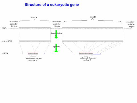
Structure of a eukaryotic gene
UTR = UnTranslated Region = part of mRNA that is not translatedCDS = CcoDing Sequence = part of mRNA (exon) that is translated
Region
zwischen−genische
Region
zwischen−genische
Region
zwischen−genische
Gen A
atgtccttttttctagtcatagtcagataa
Transkription
Spleißen
atgtatgagggagcggtgctctcacagtgaggatga
DNA
prä−mRNA
mRNA
Gen B
1:1
von Gen Akodierende Sequenz
von Gen Bkodierende Sequenz
cgagucaagguguaggcaauguccuuuuuucuagucaugguuggcaaacagugggaucc
...actaatagacatctatttcgagtcaaggtgtaggcaatgtccttttttctagtcatggttggcaaacagtgggatcctgagagtcagataattgaattggctctgcctttaattatttgttcaagcaagcccctgtccctttaggtgggaatatgtatgagggaccatatttggggttctggtagctccacagggatgcggtgatgagcgctgaatttatgacgtactag...
gcucugccuuuaauuauuuguucaagcaagccccugucccuuuaggugggaauauguaugagggaccauauuugggguucugguagcuccacagggaugcggugaugagcgcugaa
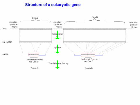
Structure of a eukaryotic gene
UTR = UnTranslated Region = part of mRNA that is not translatedCDS = CcoDing Sequence = part of mRNA (exon) that is translated
Region
zwischen−genische
Region
zwischen−genische
Region
zwischen−genische
Gen A
atgtccttttttctagtcatagtcagataa
Protein A
Transkription
Spleißen
atgtatgagggagcggtgctctcacagtgaggatga
Protein B
DNA
prä−mRNA
mRNA
Gen B
Translation und Faltung
1:1
von Gen Akodierende Sequenz
von Gen Bkodierende Sequenz
cgagucaagguguaggcaauguccuuuuuucuagucaugguuggcaaacagugggaucc
...actaatagacatctatttcgagtcaaggtgtaggcaatgtccttttttctagtcatggttggcaaacagtgggatcctgagagtcagataattgaattggctctgcctttaattatttgttcaagcaagcccctgtccctttaggtgggaatatgtatgagggaccatatttggggttctggtagctccacagggatgcggtgatgagcgctgaatttatgacgtactag...
gcucugccuuuaauuauuuguucaagcaagccccugucccuuuaggugggaauauguaugagggaccauauuugggguucugguagcuccacagggaugcggugaugagcgcugaa
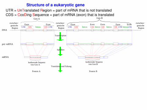
Structure of a eukaryotic geneUTR = UnTranslated Region = part of mRNA that is not translatedCDS = CcoDing Sequence = part of mRNA (exon) that is translated
Region
zwischen−genische
Region
zwischen−genische
Region
zwischen−genische
Gen A
Intron
atgtccttttttctagtcatagtcagataa
Protein A
Transkription
Spleißen
Intron
atgtatgagggagcggtgctctcacagtgaggatga
Protein B
DNA
prä−mRNA
mRNA
UTR UTR UTR UTRUTR Intron
Gen B
Translation und Faltung
1:1
CDS CDS CDS CDSIntron IntronExon Exon Exon ExonExonExonExon
CDSCDS
von Gen A von Gen Bkodierende Sequenzkodierende Sequenz
cgagucaagguguaggcaauguccuuuuuucuagucaugguuggcaaacagugggaucc
...actaatagacatctatttcgagtcaaggtgtaggcaatgtccttttttctagtcatggttggcaaacagtgggatcctgagagtcagataattgaattggctctgcctttaattatttgttcaagcaagcccctgtccctttaggtgggaatatgtatgagggaccatatttggggttctggtagctccacagggatgcggtgatgagcgctgaatttatgacgtactag...
gcucugccuuuaauuauuuguucaagcaagccccugucccuuuaggugggaauauguaugagggaccauauuugggguucugguagcuccacagggaugcggugaugagcgcugaa
Structure of a eukaryotic gene
UTR = UnTranslated Region = part of mRNA that is not translatedCDS = CcoDing Sequence = part of mRNA (exon) that is translated
Region
zwischen−genische
Region
zwischen−genische
Region
zwischen−genische
Gen A
Intron
atgtccttttttctagtcatagtcagataa
Protein A
Transkription
Spleißen
Intron
atgtatgagggagcggtgctctcacagtgaggatga
Protein B
DNA
prä−mRNA
mRNA
UTR UTR UTR UTRUTR Intron
Gen B
Translation und Faltung
1:1
CDS CDS CDS CDSIntron IntronExon Exon Exon ExonExonExonExon
CDSCDS
von Gen A von Gen Bkodierende Sequenzkodierende Sequenz
cgagucaagguguaggcaauguccuuuuuucuagucaugguuggcaaacagugggaucc
...actaatagacatctatttcgagtcaaggtgtaggcaatgtccttttttctagtcatggttggcaaacagtgggatcctgagagtcagataattgaattggctctgcctttaattatttgttcaagcaagcccctgtccctttaggtgggaatatgtatgagggaccatatttggggttctggtagctccacagggatgcggtgatgagcgctgaatttatgacgtactag...
gcucugccuuuaauuauuuguucaagcaagccccugucccuuuaggugggaauauguaugagggaccauauuugggguucugguagcuccacagggaugcggugaugagcgcugaa
Genvorhersage
Dr. Mario Stanke
Lernziele / Study Aims
Introduction toGene-Finding-ProblemWhat Do Genes Look Like?
Statistical Features ofGenes
Gene Finding ThroughExon-ChainingThe One-DimensionalChaining Problem
Exon-Chaining Algorithm
Gene Finding withHMMsGeneralized HMMs
Model Design
Training
Pair Hidden MarkovModelsDefinitions
Application: ComparativeGene Prediction
1.8
Translation
atg tat gag ... gga tga
Kodons
M Y EAminosäuren
Sequenz von G
DNA−Sequenzkodierende
Translation
Faltung
...
nur am Ende
Protein
eines von 3 Stopp−Kodons,
“universeller”genetischer Code
Kodon Amino-(DNA) säureaaa 7→ Kaac 7→ Naag 7→ Kaat 7→ N
.
.
.
.
.
.atg 7→ M
.
.
.
.
.
.61 20Kodons Amino-
säuren

Genvorhersage
Dr. Mario Stanke
Lernziele / Study Aims
Introduction toGene-Finding-ProblemWhat Do Genes Look Like?
Statistical Features ofGenes
Gene Finding ThroughExon-ChainingThe One-DimensionalChaining Problem
Exon-Chaining Algorithm
Gene Finding withHMMsGeneralized HMMs
Model Design
Training
Pair Hidden MarkovModelsDefinitions
Application: ComparativeGene Prediction
1.8
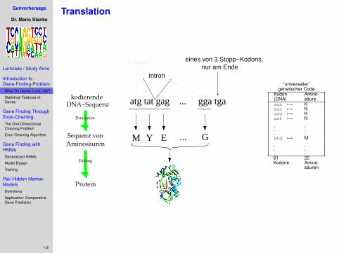
Translation
Intron
atg tat gag ... gga tga
M Y EAminosäuren
Sequenz von G
DNA−Sequenzkodierende
Translation
Faltung
...
nur am Ende
Protein
eines von 3 Stopp−Kodons,Kodons
“universeller”genetischer Code
Kodon Amino-(DNA) säureaaa 7→ Kaac 7→ Naag 7→ Kaat 7→ N
.
.
.
.
.
.atg 7→ M
.
.
.
.
.
.61 20Kodons Amino-
säuren

Genvorhersage
Dr. Mario Stanke
Lernziele / Study Aims
Introduction toGene-Finding-ProblemWhat Do Genes Look Like?
Statistical Features ofGenes
Gene Finding ThroughExon-ChainingThe One-DimensionalChaining Problem
Exon-Chaining Algorithm
Gene Finding withHMMsGeneralized HMMs
Model Design
Training
Pair Hidden MarkovModelsDefinitions
Application: ComparativeGene Prediction
1.8
Translation
Intron
atg tat gag ... gga tga
M Y EAminosäuren
Sequenz von G
DNA−Sequenzkodierende
Translation
Faltung
...
nur am Ende
Protein
eines von 3 Stopp−Kodons,Kodons
“universeller”genetischer Code
Kodon Amino-(DNA) säureaaa 7→ Kaac 7→ Naag 7→ Kaat 7→ N
.
.
.
.
.
.atg 7→ M
.
.
.
.
.
.61 20Kodons Amino-
säuren
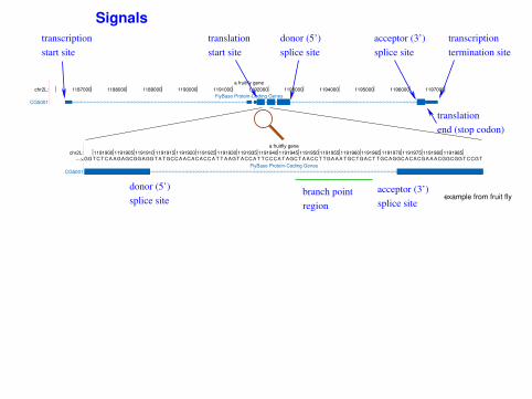
Signals
chr2L:
a fruitfly gene
1187000 1188000 1189000 1190000 1191000 1192000 1193000 1194000 1195000 1196000 1197000
FlyBase Protein-Coding Genes
CG5001
chr2L:
--->
a fruitfly gene
1191900 1191905 1191910 1191915 1191920 1191925 1191930 1191935 1191940 1191945 1191950 1191955 1191960 1191965 1191970 1191975 1191980 1191985
GGT C T CA AGAGCGGAGGT A TGCCA ACACACCA T T A AGT ACCA T T CCCA T AGC T A ACC T TGA A A TGC TGAC T TGCAGGCACACGA A ACGGCGGT CCGT
FlyBase Protein-Coding Genes
CG5001
donor (5’)
splice site
transcription
start site
transcription
termination site
donor (5’)
splice site
acceptor (3’)
splice site
acceptor (3’)
splice site
branch point
region
translation
start site
translation
end (stop codon)
example from fruit fly
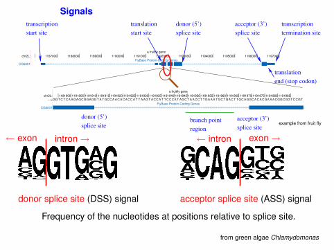
intron→← exon
donor splice site (DSS) signal
exon→← intron
acceptor splice site (ASS) signal
Frequency of the nucleotides at positions relative to splice site.
from green algae Chlamydomonas
Signals
chr2L:
a fruitfly gene
1187000 1188000 1189000 1190000 1191000 1192000 1193000 1194000 1195000 1196000 1197000
FlyBase Protein-Coding Genes
CG5001
chr2L:
--->
a fruitfly gene
1191900 1191905 1191910 1191915 1191920 1191925 1191930 1191935 1191940 1191945 1191950 1191955 1191960 1191965 1191970 1191975 1191980 1191985
GGT C T CA AGAGCGGAGGT A TGCCA ACACACCA T T A AGT ACCA T T CCCA T AGC T A ACC T TGA A A TGC TGAC T TGCAGGCACACGA A ACGGCGGT CCGT
FlyBase Protein-Coding Genes
CG5001
donor (5’)
splice site
transcription
start site
transcription
termination site
donor (5’)
splice site
acceptor (3’)
splice site
acceptor (3’)
splice site
branch point
region
translation
start site
translation
end (stop codon)
example from fruit fly
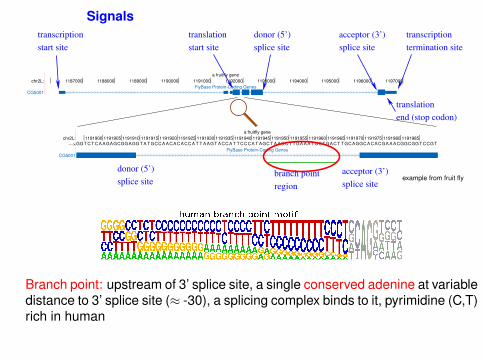
Branch point: upstream of 3’ splice site, a single conserved adenine at variabledistance to 3’ splice site (≈ -30), a splicing complex binds to it, pyrimidine (C,T)rich in human

Signals
chr2L:
a fruitfly gene
1187000 1188000 1189000 1190000 1191000 1192000 1193000 1194000 1195000 1196000 1197000
FlyBase Protein-Coding Genes
CG5001
chr2L:
--->
a fruitfly gene
1191900 1191905 1191910 1191915 1191920 1191925 1191930 1191935 1191940 1191945 1191950 1191955 1191960 1191965 1191970 1191975 1191980 1191985
GGT C T CA AGAGCGGAGGT A TGCCA ACACACCA T T A AGT ACCA T T CCCA T AGC T A ACC T TGA A A TGC TGAC T TGCAGGCACACGA A ACGGCGGT CCGT
FlyBase Protein-Coding Genes
CG5001
donor (5’)
splice site
transcription
start site
transcription
termination site
donor (5’)
splice site
acceptor (3’)
splice site
acceptor (3’)
splice site
branch point
region
translation
start site
translation
end (stop codon)
example from fruit fly
Transcription start site: Transcription from DNA to RNA by RNA polymerasestarts here facilitated by promoter elements.Promoter elements are diverse and their profiles tend to contain little info:• diverse transcription factor binding sites at very variable positions• sometimes TATA-box• “CpG islands”
Signals
chr2L:
a fruitfly gene
1187000 1188000 1189000 1190000 1191000 1192000 1193000 1194000 1195000 1196000 1197000
FlyBase Protein-Coding Genes
CG5001
chr2L:
--->
a fruitfly gene
1191900 1191905 1191910 1191915 1191920 1191925 1191930 1191935 1191940 1191945 1191950 1191955 1191960 1191965 1191970 1191975 1191980 1191985
GGT C T CA AGAGCGGAGGT A TGCCA ACACACCA T T A AGT ACCA T T CCCA T AGC T A ACC T TGA A A TGC TGAC T TGCAGGCACACGA A ACGGCGGT CCGT
FlyBase Protein-Coding Genes
CG5001
donor (5’)
splice site
transcription
start site
transcription
termination site
donor (5’)
splice site
acceptor (3’)
splice site
acceptor (3’)
splice site
branch point
region
translation
start site
translation
end (stop codon)
example from fruit fly
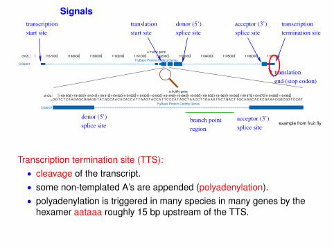
Transcription termination site (TTS):• cleavage of the transcript.• some non-templated A’s are appended (polyadenylation).• polyadenylation is triggered in many species in many genes by the
hexamer aataaa roughly 15 bp upstream of the TTS.

Signals
chr2L:
a fruitfly gene
1187000 1188000 1189000 1190000 1191000 1192000 1193000 1194000 1195000 1196000 1197000
FlyBase Protein-Coding Genes
CG5001
chr2L:
--->
a fruitfly gene
1191900 1191905 1191910 1191915 1191920 1191925 1191930 1191935 1191940 1191945 1191950 1191955 1191960 1191965 1191970 1191975 1191980 1191985
GGT C T CA AGAGCGGAGGT A TGCCA ACACACCA T T A AGT ACCA T T CCCA T AGC T A ACC T TGA A A TGC TGAC T TGCAGGCACACGA A ACGGCGGT CCGT
FlyBase Protein-Coding Genes
CG5001
donor (5’)
splice site
transcription
start site
transcription
termination site
donor (5’)
splice site
acceptor (3’)
splice site
acceptor (3’)
splice site
branch point
region
translation
start site
translation
end (stop codon)
example from fruit fly
Start and stop codon:• start codon: ATG• stop codons: TAA, TAG, TGA
In some species the genetic code is altered and a “stop codon” isactually coding for an amino acid.
Genvorhersage
Dr. Mario Stanke
Lernziele / Study Aims
Introduction toGene-Finding-ProblemWhat Do Genes Look Like?
Statistical Features ofGenes
Gene Finding ThroughExon-ChainingThe One-DimensionalChaining Problem
Exon-Chaining Algorithm
Gene Finding withHMMsGeneralized HMMs
Model Design
Training
Pair Hidden MarkovModelsDefinitions
Application: ComparativeGene Prediction
1.10
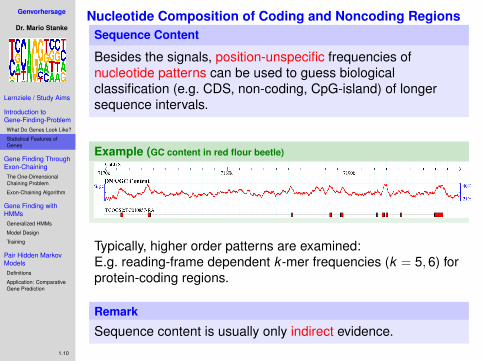
Nucleotide Composition of Coding and Noncoding RegionsSequence Content
Besides the signals, position-unspecific frequencies ofnucleotide patterns can be used to guess biologicalclassification (e.g. CDS, non-coding, CpG-island) of longersequence intervals.
Example (GC content in red flour beetle)
Typically, higher order patterns are examined:E.g. reading-frame dependent k -mer frequencies (k = 5,6) forprotein-coding regions.
Remark
Sequence content is usually only indirect evidence.
Genvorhersage
Dr. Mario Stanke
Lernziele / Study Aims
Introduction toGene-Finding-ProblemWhat Do Genes Look Like?
Statistical Features ofGenes
Gene Finding ThroughExon-ChainingThe One-DimensionalChaining Problem
Exon-Chaining Algorithm
Gene Finding withHMMsGeneralized HMMs
Model Design
Training
Pair Hidden MarkovModelsDefinitions
Application: ComparativeGene Prediction
1.11
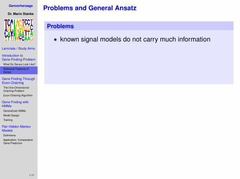
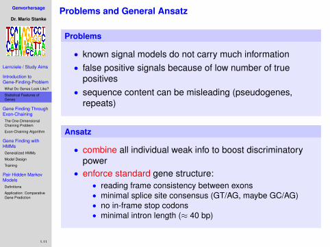
Problems and General Ansatz
Problems
• known signal models do not carry much information
• false positive signals because of low number of truepositives
• sequence content can be misleading (pseudogenes,repeats)
Ansatz
• combine all individual weak info to boost discriminatorypower
• enforce standard gene structure:• reading frame consistency between exons• minimal splice site consensus (GT/AG, maybe GC/AG)• no in-frame stop codons• minimal intron length (≈ 40 bp)
Genvorhersage
Dr. Mario Stanke
Lernziele / Study Aims
Introduction toGene-Finding-ProblemWhat Do Genes Look Like?
Statistical Features ofGenes
Gene Finding ThroughExon-ChainingThe One-DimensionalChaining Problem
Exon-Chaining Algorithm
Gene Finding withHMMsGeneralized HMMs
Model Design
Training
Pair Hidden MarkovModelsDefinitions
Application: ComparativeGene Prediction
1.11
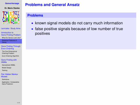
Problems and General Ansatz
Problems
• known signal models do not carry much information• false positive signals because of low number of true
positives
• sequence content can be misleading (pseudogenes,repeats)
Ansatz
• combine all individual weak info to boost discriminatorypower
• enforce standard gene structure:• reading frame consistency between exons• minimal splice site consensus (GT/AG, maybe GC/AG)• no in-frame stop codons• minimal intron length (≈ 40 bp)
Genvorhersage
Dr. Mario Stanke
Lernziele / Study Aims
Introduction toGene-Finding-ProblemWhat Do Genes Look Like?
Statistical Features ofGenes
Gene Finding ThroughExon-ChainingThe One-DimensionalChaining Problem
Exon-Chaining Algorithm
Gene Finding withHMMsGeneralized HMMs
Model Design
Training
Pair Hidden MarkovModelsDefinitions
Application: ComparativeGene Prediction
1.11
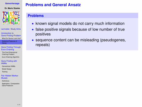
Problems and General Ansatz
Problems
• known signal models do not carry much information• false positive signals because of low number of true
positives• sequence content can be misleading (pseudogenes,
repeats)
Ansatz
• combine all individual weak info to boost discriminatorypower
• enforce standard gene structure:• reading frame consistency between exons• minimal splice site consensus (GT/AG, maybe GC/AG)• no in-frame stop codons• minimal intron length (≈ 40 bp)
Genvorhersage
Dr. Mario Stanke
Lernziele / Study Aims
Introduction toGene-Finding-ProblemWhat Do Genes Look Like?
Statistical Features ofGenes
Gene Finding ThroughExon-ChainingThe One-DimensionalChaining Problem
Exon-Chaining Algorithm
Gene Finding withHMMsGeneralized HMMs
Model Design
Training
Pair Hidden MarkovModelsDefinitions
Application: ComparativeGene Prediction
1.11
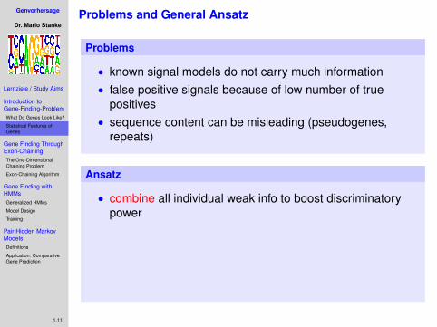
Problems and General Ansatz
Problems
• known signal models do not carry much information• false positive signals because of low number of true
positives• sequence content can be misleading (pseudogenes,
repeats)
Ansatz
• combine all individual weak info to boost discriminatorypower
• enforce standard gene structure:• reading frame consistency between exons• minimal splice site consensus (GT/AG, maybe GC/AG)• no in-frame stop codons• minimal intron length (≈ 40 bp)
Genvorhersage
Dr. Mario Stanke
Lernziele / Study Aims
Introduction toGene-Finding-ProblemWhat Do Genes Look Like?
Statistical Features ofGenes
Gene Finding ThroughExon-ChainingThe One-DimensionalChaining Problem
Exon-Chaining Algorithm
Gene Finding withHMMsGeneralized HMMs
Model Design
Training
Pair Hidden MarkovModelsDefinitions
Application: ComparativeGene Prediction
1.11
Problems and General Ansatz
Problems
• known signal models do not carry much information• false positive signals because of low number of true
positives• sequence content can be misleading (pseudogenes,
repeats)
Ansatz
• combine all individual weak info to boost discriminatorypower
• enforce standard gene structure:• reading frame consistency between exons• minimal splice site consensus (GT/AG, maybe GC/AG)• no in-frame stop codons• minimal intron length (≈ 40 bp)
Genvorhersage
Dr. Mario Stanke
Lernziele / Study Aims
Introduction toGene-Finding-ProblemWhat Do Genes Look Like?
Statistical Features ofGenes
Gene Finding ThroughExon-ChainingThe One-DimensionalChaining Problem
Exon-Chaining Algorithm
Gene Finding withHMMsGeneralized HMMs
Model Design
Training
Pair Hidden MarkovModelsDefinitions
Application: ComparativeGene Prediction
1.12
1 Introduction to Gene-Finding-ProblemWhat Do Genes Look Like?Statistical Features of Genes
2 Gene Finding Through Exon-ChainingThe One-Dimensional Chaining ProblemExon-Chaining Algorithm
3 Gene Finding with HMMsGeneralized HMMsModel DesignTraining
4 Pair Hidden Markov ModelsDefinitionsApplication: Comparative Gene Prediction

Genvorhersage
Dr. Mario Stanke
Lernziele / Study Aims
Introduction toGene-Finding-ProblemWhat Do Genes Look Like?
Statistical Features ofGenes
Gene Finding ThroughExon-ChainingThe One-DimensionalChaining Problem
Exon-Chaining Algorithm
Gene Finding withHMMsGeneralized HMMs
Model Design
Training
Pair Hidden MarkovModelsDefinitions
Application: ComparativeGene Prediction
1.13
This Section Also in My German Script
http://gobics.de/mario/genomanalyse/script.pdfpages 28-32

Genvorhersage
Dr. Mario Stanke
Lernziele / Study Aims
Introduction toGene-Finding-ProblemWhat Do Genes Look Like?
Statistical Features ofGenes
Gene Finding ThroughExon-ChainingThe One-DimensionalChaining Problem
Exon-Chaining Algorithm
Gene Finding withHMMsGeneralized HMMs
Model Design
Training
Pair Hidden MarkovModelsDefinitions
Application: ComparativeGene Prediction
1.14
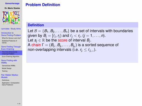
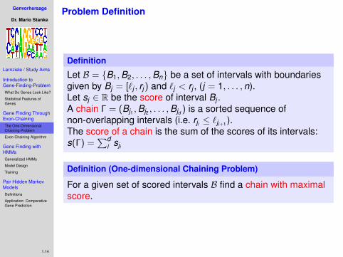
Problem Definition
Definition
Let B = {B1,B2, . . . ,Bn} be a set of intervals with boundariesgiven by Bj = [`j , rj ) and `j < rj , (j = 1, . . . ,n).Let sj ∈ R be the score of interval Bj .
A chain Γ = (Bj1 ,Bj2 , . . . ,Bjd ) is a sorted sequence ofnon-overlapping intervals (i.e. rji ≤ `ji+1 ).The score of a chain is the sum of the scores of its intervals:s(Γ) =
∑di sji
Definition (One-dimensional Chaining Problem)
For a given set of scored intervals B find a chain with maximalscore.
Genvorhersage
Dr. Mario Stanke
Lernziele / Study Aims
Introduction toGene-Finding-ProblemWhat Do Genes Look Like?
Statistical Features ofGenes
Gene Finding ThroughExon-ChainingThe One-DimensionalChaining Problem
Exon-Chaining Algorithm
Gene Finding withHMMsGeneralized HMMs
Model Design
Training
Pair Hidden MarkovModelsDefinitions
Application: ComparativeGene Prediction
1.14
Problem Definition
Definition
Let B = {B1,B2, . . . ,Bn} be a set of intervals with boundariesgiven by Bj = [`j , rj ) and `j < rj , (j = 1, . . . ,n).Let sj ∈ R be the score of interval Bj .A chain Γ = (Bj1 ,Bj2 , . . . ,Bjd ) is a sorted sequence ofnon-overlapping intervals (i.e. rji ≤ `ji+1 ).
The score of a chain is the sum of the scores of its intervals:s(Γ) =
∑di sji
Definition (One-dimensional Chaining Problem)
For a given set of scored intervals B find a chain with maximalscore.

Genvorhersage
Dr. Mario Stanke
Lernziele / Study Aims
Introduction toGene-Finding-ProblemWhat Do Genes Look Like?
Statistical Features ofGenes
Gene Finding ThroughExon-ChainingThe One-DimensionalChaining Problem
Exon-Chaining Algorithm
Gene Finding withHMMsGeneralized HMMs
Model Design
Training
Pair Hidden MarkovModelsDefinitions
Application: ComparativeGene Prediction
1.14
Problem Definition
Definition
Let B = {B1,B2, . . . ,Bn} be a set of intervals with boundariesgiven by Bj = [`j , rj ) and `j < rj , (j = 1, . . . ,n).Let sj ∈ R be the score of interval Bj .A chain Γ = (Bj1 ,Bj2 , . . . ,Bjd ) is a sorted sequence ofnon-overlapping intervals (i.e. rji ≤ `ji+1 ).The score of a chain is the sum of the scores of its intervals:s(Γ) =
∑di sji
Definition (One-dimensional Chaining Problem)
For a given set of scored intervals B find a chain with maximalscore.
Genvorhersage
Dr. Mario Stanke
Lernziele / Study Aims
Introduction toGene-Finding-ProblemWhat Do Genes Look Like?
Statistical Features ofGenes
Gene Finding ThroughExon-ChainingThe One-DimensionalChaining Problem
Exon-Chaining Algorithm
Gene Finding withHMMsGeneralized HMMs
Model Design
Training
Pair Hidden MarkovModelsDefinitions
Application: ComparativeGene Prediction
1.15
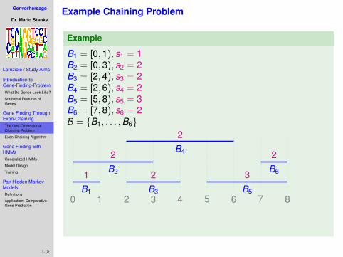
Example Chaining Problem
Example
B1 = [0,1), s1 = 1B2 = [0,3), s2 = 2B3 = [2,4), s3 = 2B4 = [2,6), s4 = 2B5 = [5,8), s5 = 3B6 = [7,8), s6 = 2B = {B1, . . . ,B6}
0 1 2 3 4 5 6 7 8B1
1B2
2
B3
2
B4
2
B5
3 B6
2
Γ = (B1,B3,B5) is the chain with maximal score.

Genvorhersage
Dr. Mario Stanke
Lernziele / Study Aims
Introduction toGene-Finding-ProblemWhat Do Genes Look Like?
Statistical Features ofGenes
Gene Finding ThroughExon-ChainingThe One-DimensionalChaining Problem
Exon-Chaining Algorithm
Gene Finding withHMMsGeneralized HMMs
Model Design
Training
Pair Hidden MarkovModelsDefinitions
Application: ComparativeGene Prediction
1.15
Example Chaining Problem
Example
B1 = [0,1), s1 = 1B2 = [0,3), s2 = 2B3 = [2,4), s3 = 2B4 = [2,6), s4 = 2B5 = [5,8), s5 = 3B6 = [7,8), s6 = 2B = {B1, . . . ,B6}
0 1 2 3 4 5 6 7 8B1
1 B2
2
B3
2
B4
2
B5
3 B6
2
Γ = (B1,B3,B5) is the chain with maximal score.

Genvorhersage
Dr. Mario Stanke
Lernziele / Study Aims
Introduction toGene-Finding-ProblemWhat Do Genes Look Like?
Statistical Features ofGenes
Gene Finding ThroughExon-ChainingThe One-DimensionalChaining Problem
Exon-Chaining Algorithm
Gene Finding withHMMsGeneralized HMMs
Model Design
Training
Pair Hidden MarkovModelsDefinitions
Application: ComparativeGene Prediction
1.16
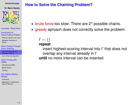
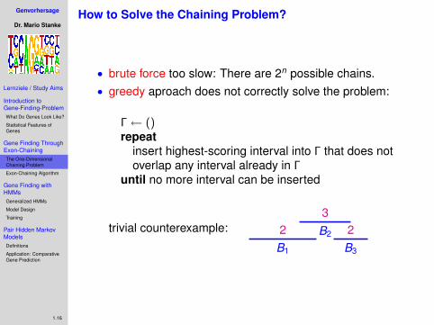
How to Solve the Chaining Problem?
• brute force too slow: There are 2n possible chains.
• greedy aproach does not correctly solve the problem:
Γ← ()repeat
insert highest-scoring interval into Γ that does notoverlap any interval already in Γ
until no more interval can be inserted
trivial counterexample:
B1
2 B2
3
B3
2
Genvorhersage
Dr. Mario Stanke
Lernziele / Study Aims
Introduction toGene-Finding-ProblemWhat Do Genes Look Like?
Statistical Features ofGenes
Gene Finding ThroughExon-ChainingThe One-DimensionalChaining Problem
Exon-Chaining Algorithm
Gene Finding withHMMsGeneralized HMMs
Model Design
Training
Pair Hidden MarkovModelsDefinitions
Application: ComparativeGene Prediction
1.16
How to Solve the Chaining Problem?
• brute force too slow: There are 2n possible chains.• greedy aproach does not correctly solve the problem:
Γ← ()repeat
insert highest-scoring interval into Γ that does notoverlap any interval already in Γ
until no more interval can be inserted
trivial counterexample:
B1
2 B2
3
B3
2

Genvorhersage
Dr. Mario Stanke
Lernziele / Study Aims
Introduction toGene-Finding-ProblemWhat Do Genes Look Like?
Statistical Features ofGenes
Gene Finding ThroughExon-ChainingThe One-DimensionalChaining Problem
Exon-Chaining Algorithm
Gene Finding withHMMsGeneralized HMMs
Model Design
Training
Pair Hidden MarkovModelsDefinitions
Application: ComparativeGene Prediction
1.17
Chaining Algorithm
One-Dimensional Chaining Algorithm
1: P ← sort {`1, r1, `2, r2, . . . , `n, rn} increasingly2: S ← q ← q1 ← · · · ← qn ← S1 ← · · ·Sn ← 03: while P not empty do4: b ← remove smallest element in P5: for all j such that rj = b do6: if Sj > S then7: S ← Sj8: q ← j9: end if
10: end for11: for all j such that `j = b do12: Sj ← sj + S13: qj ← q14: end for15: end while16: output S as score of best chain
Genvorhersage
Dr. Mario Stanke
Lernziele / Study Aims
Introduction toGene-Finding-ProblemWhat Do Genes Look Like?
Statistical Features ofGenes
Gene Finding ThroughExon-ChainingThe One-DimensionalChaining Problem
Exon-Chaining Algorithm
Gene Finding withHMMsGeneralized HMMs
Model Design
Training
Pair Hidden MarkovModelsDefinitions
Application: ComparativeGene Prediction
1.18
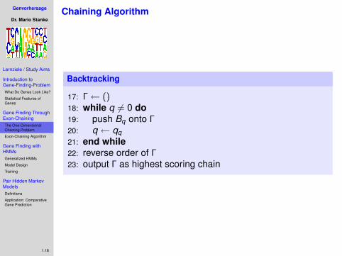
Chaining Algorithm
Backtracking
17: Γ← ()18: while q 6= 0 do19: push Bq onto Γ20: q ← qq21: end while22: reverse order of Γ23: output Γ as highest scoring chain
Genvorhersage
Dr. Mario Stanke
Lernziele / Study Aims
Introduction toGene-Finding-ProblemWhat Do Genes Look Like?
Statistical Features ofGenes
Gene Finding ThroughExon-ChainingThe One-DimensionalChaining Problem
Exon-Chaining Algorithm
Gene Finding withHMMsGeneralized HMMs
Model Design
Training
Pair Hidden MarkovModelsDefinitions
Application: ComparativeGene Prediction
1.19
Correctness
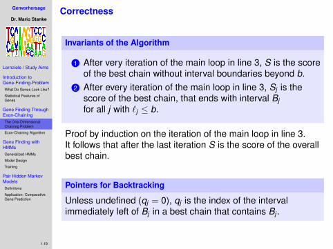
Invariants of the Algorithm
1 After very iteration of the main loop in line 3, S is the scoreof the best chain without interval boundaries beyond b.
2 After every iteration of the main loop in line 3, Sj is thescore of the best chain, that ends with interval Bjfor all j with `j ≤ b.
Proof by induction on the iteration of the main loop in line 3.It follows that after the last iteration S is the score of the overallbest chain.
Pointers for Backtracking
Unless undefined (qj = 0), qj is the index of the intervalimmediately left of Bj in a best chain that contains Bj .
Genvorhersage
Dr. Mario Stanke
Lernziele / Study Aims
Introduction toGene-Finding-ProblemWhat Do Genes Look Like?
Statistical Features ofGenes
Gene Finding ThroughExon-ChainingThe One-DimensionalChaining Problem
Exon-Chaining Algorithm
Gene Finding withHMMsGeneralized HMMs
Model Design
Training
Pair Hidden MarkovModelsDefinitions
Application: ComparativeGene Prediction
1.20
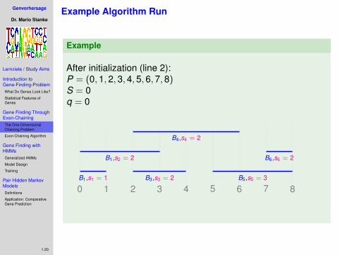
Example Algorithm Run
Example
.After initialization (line 2):P = (0,1,2,3,4,5,6,7,8)S = 0q = 0
0 1 2 3 4 5 6 7 8B1,s1 = 1
B1,s2 = 2
B3,s3 = 2
B4,s4 = 2
B5,s5 = 3
B6,s6 = 2
Genvorhersage
Dr. Mario Stanke
Lernziele / Study Aims
Introduction toGene-Finding-ProblemWhat Do Genes Look Like?
Statistical Features ofGenes
Gene Finding ThroughExon-ChainingThe One-DimensionalChaining Problem
Exon-Chaining Algorithm
Gene Finding withHMMsGeneralized HMMs
Model Design
Training
Pair Hidden MarkovModelsDefinitions
Application: ComparativeGene Prediction
1.20
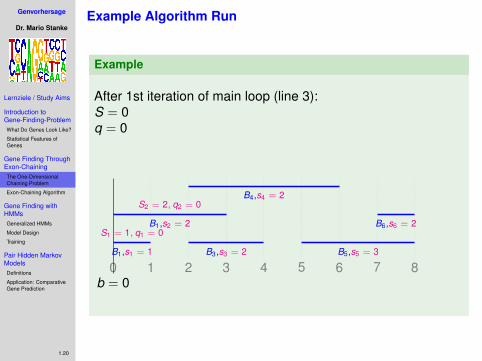
Example Algorithm Run
Example
.After 1st iteration of main loop (line 3):S = 0q = 0
0 1 2 3 4 5 6 7 8B1,s1 = 1
S1 = 1, q1 = 0B1,s2 = 2
S2 = 2, q2 = 0
B3,s3 = 2
B4,s4 = 2
B5,s5 = 3
B6,s6 = 2
b = 0
Genvorhersage
Dr. Mario Stanke
Lernziele / Study Aims
Introduction toGene-Finding-ProblemWhat Do Genes Look Like?
Statistical Features ofGenes
Gene Finding ThroughExon-ChainingThe One-DimensionalChaining Problem
Exon-Chaining Algorithm
Gene Finding withHMMsGeneralized HMMs
Model Design
Training
Pair Hidden MarkovModelsDefinitions
Application: ComparativeGene Prediction
1.20
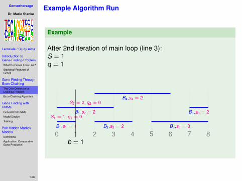
Example Algorithm Run
Example
.After 2nd iteration of main loop (line 3):S = 1q = 1
0 1 2 3 4 5 6 7 8B1,s1 = 1
S1 = 1, q1 = 0B1,s2 = 2
S2 = 2, q2 = 0
B3,s3 = 2
B4,s4 = 2
B5,s5 = 3
B6,s6 = 2
b = 1
Genvorhersage
Dr. Mario Stanke
Lernziele / Study Aims
Introduction toGene-Finding-ProblemWhat Do Genes Look Like?
Statistical Features ofGenes
Gene Finding ThroughExon-ChainingThe One-DimensionalChaining Problem
Exon-Chaining Algorithm
Gene Finding withHMMsGeneralized HMMs
Model Design
Training
Pair Hidden MarkovModelsDefinitions
Application: ComparativeGene Prediction
1.20
Example Algorithm Run
Example
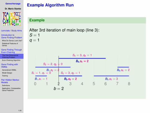
.After 3rd iteration of main loop (line 3):S = 1q = 1
0 1 2 3 4 5 6 7 8B1,s1 = 1
S1 = 1, q1 = 0B1,s2 = 2
S2 = 2, q2 = 0
B3,s3 = 2B3,s3 = 2
S3 = 3, q3 = 1
B4,s4 = 2B4,s4 = 2
S4 = 3, q4 = 1
B5,s5 = 3
B6,s6 = 2
b = 2
Genvorhersage
Dr. Mario Stanke
Lernziele / Study Aims
Introduction toGene-Finding-ProblemWhat Do Genes Look Like?
Statistical Features ofGenes
Gene Finding ThroughExon-ChainingThe One-DimensionalChaining Problem
Exon-Chaining Algorithm
Gene Finding withHMMsGeneralized HMMs
Model Design
Training
Pair Hidden MarkovModelsDefinitions
Application: ComparativeGene Prediction
1.20
Example Algorithm Run
Example
.After 4th iteration of main loop (line 3):S = 2q = 2
0 1 2 3 4 5 6 7 8B1,s1 = 1
S1 = 1, q1 = 0B1,s2 = 2
S2 = 2, q2 = 0
B3,s3 = 2B3,s3 = 2
S3 = 3, q3 = 1
B4,s4 = 2B4,s4 = 2
S4 = 3, q4 = 1
B5,s5 = 3
B6,s6 = 2
b = 3
Genvorhersage
Dr. Mario Stanke
Lernziele / Study Aims
Introduction toGene-Finding-ProblemWhat Do Genes Look Like?
Statistical Features ofGenes
Gene Finding ThroughExon-ChainingThe One-DimensionalChaining Problem
Exon-Chaining Algorithm
Gene Finding withHMMsGeneralized HMMs
Model Design
Training
Pair Hidden MarkovModelsDefinitions
Application: ComparativeGene Prediction
1.20
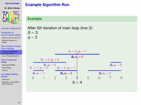
Example Algorithm Run
Example
.After 5th iteration of main loop (line 3):S = 3q = 3
0 1 2 3 4 5 6 7 8B1,s1 = 1
S1 = 1, q1 = 0B1,s2 = 2
S2 = 2, q2 = 0
B3,s3 = 2B3,s3 = 2
S3 = 3, q3 = 1
B4,s4 = 2B4,s4 = 2
S4 = 3, q4 = 1
B5,s5 = 3
B6,s6 = 2
b = 4
Genvorhersage
Dr. Mario Stanke
Lernziele / Study Aims
Introduction toGene-Finding-ProblemWhat Do Genes Look Like?
Statistical Features ofGenes
Gene Finding ThroughExon-ChainingThe One-DimensionalChaining Problem
Exon-Chaining Algorithm
Gene Finding withHMMsGeneralized HMMs
Model Design
Training
Pair Hidden MarkovModelsDefinitions
Application: ComparativeGene Prediction
1.20
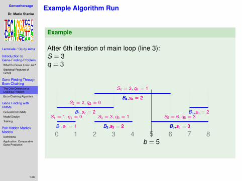
Example Algorithm Run
Example
.After 6th iteration of main loop (line 3):S = 3q = 3
0 1 2 3 4 5 6 7 8B1,s1 = 1
S1 = 1, q1 = 0B1,s2 = 2
S2 = 2, q2 = 0
B3,s3 = 2B3,s3 = 2
S3 = 3, q3 = 1
B4,s4 = 2B4,s4 = 2
S4 = 3, q4 = 1
B5,s5 = 3B5,s5 = 3
S5 = 6, q5 = 3B6,s6 = 2
b = 5
Genvorhersage
Dr. Mario Stanke
Lernziele / Study Aims
Introduction toGene-Finding-ProblemWhat Do Genes Look Like?
Statistical Features ofGenes
Gene Finding ThroughExon-ChainingThe One-DimensionalChaining Problem
Exon-Chaining Algorithm
Gene Finding withHMMsGeneralized HMMs
Model Design
Training
Pair Hidden MarkovModelsDefinitions
Application: ComparativeGene Prediction
1.20
Example Algorithm Run
Example
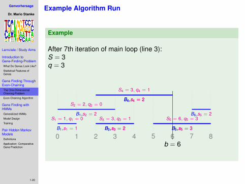
.After 7th iteration of main loop (line 3):S = 3q = 3
0 1 2 3 4 5 6 7 8B1,s1 = 1
S1 = 1, q1 = 0B1,s2 = 2
S2 = 2, q2 = 0
B3,s3 = 2B3,s3 = 2
S3 = 3, q3 = 1
B4,s4 = 2B4,s4 = 2
S4 = 3, q4 = 1
B5,s5 = 3B5,s5 = 3
S5 = 6, q5 = 3B6,s6 = 2
b = 6
Genvorhersage
Dr. Mario Stanke
Lernziele / Study Aims
Introduction toGene-Finding-ProblemWhat Do Genes Look Like?
Statistical Features ofGenes
Gene Finding ThroughExon-ChainingThe One-DimensionalChaining Problem
Exon-Chaining Algorithm
Gene Finding withHMMsGeneralized HMMs
Model Design
Training
Pair Hidden MarkovModelsDefinitions
Application: ComparativeGene Prediction
1.20
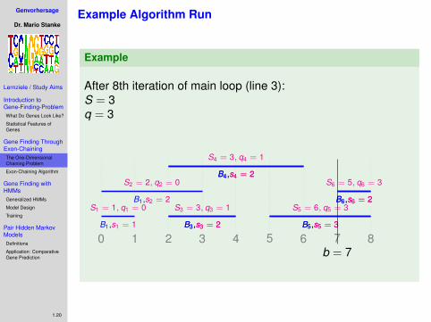
Example Algorithm Run
Example
.After 8th iteration of main loop (line 3):S = 3q = 3
0 1 2 3 4 5 6 7 8B1,s1 = 1
S1 = 1, q1 = 0B1,s2 = 2
S2 = 2, q2 = 0
B3,s3 = 2B3,s3 = 2
S3 = 3, q3 = 1
B4,s4 = 2B4,s4 = 2
S4 = 3, q4 = 1
B5,s5 = 3B5,s5 = 3
S5 = 6, q5 = 3B6,s6 = 2B6,s6 = 2
S6 = 5, q6 = 3
b = 7
Genvorhersage
Dr. Mario Stanke
Lernziele / Study Aims
Introduction toGene-Finding-ProblemWhat Do Genes Look Like?
Statistical Features ofGenes
Gene Finding ThroughExon-ChainingThe One-DimensionalChaining Problem
Exon-Chaining Algorithm
Gene Finding withHMMsGeneralized HMMs
Model Design
Training
Pair Hidden MarkovModelsDefinitions
Application: ComparativeGene Prediction
1.20
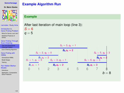
Example Algorithm Run
Example
.After last iteration of main loop (line 3):S = 6q = 5
0 1 2 3 4 5 6 7 8B1,s1 = 1
S1 = 1, q1 = 0B1,s2 = 2
S2 = 2, q2 = 0
B3,s3 = 2B3,s3 = 2
S3 = 3, q3 = 1
B4,s4 = 2B4,s4 = 2
S4 = 3, q4 = 1
B5,s5 = 3B5,s5 = 3
S5 = 6, q5 = 3B6,s6 = 2B6,s6 = 2
S6 = 5, q6 = 3
b = 8
Genvorhersage
Dr. Mario Stanke
Lernziele / Study Aims
Introduction toGene-Finding-ProblemWhat Do Genes Look Like?
Statistical Features ofGenes
Gene Finding ThroughExon-ChainingThe One-DimensionalChaining Problem
Exon-Chaining Algorithm
Gene Finding withHMMsGeneralized HMMs
Model Design
Training
Pair Hidden MarkovModelsDefinitions
Application: ComparativeGene Prediction
1.20
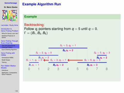
Example Algorithm Run
Example
.Backtracking:Follow qj pointers starting from q = 5 until q = 0.Γ = (B1,B3,B5)
0 1 2 3 4 5 6 7 8B1,s1 = 1
S1 = 1, q1 = 0B1,s2 = 2
S2 = 2, q2 = 0
B3,s3 = 2B3,s3 = 2
S3 = 3, q3 = 1
B4,s4 = 2B4,s4 = 2
S4 = 3, q4 = 1
B5,s5 = 3B5,s5 = 3
S5 = 6, q5 = 3B6,s6 = 2B6,s6 = 2
S6 = 5, q6 = 3

Genvorhersage
Dr. Mario Stanke
Lernziele / Study Aims
Introduction toGene-Finding-ProblemWhat Do Genes Look Like?
Statistical Features ofGenes
Gene Finding ThroughExon-ChainingThe One-DimensionalChaining Problem
Exon-Chaining Algorithm
Gene Finding withHMMsGeneralized HMMs
Model Design
Training
Pair Hidden MarkovModelsDefinitions
Application: ComparativeGene Prediction
1.21
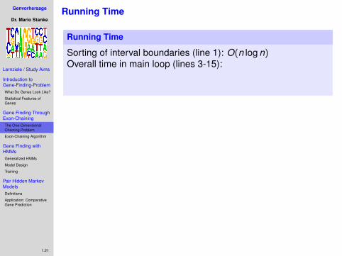
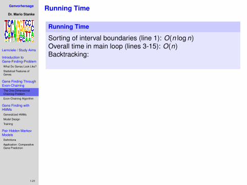
Running Time
Running Time
Sorting of interval boundaries (line 1):
O(n log n)Overall time in main loop (lines 3-15): O(n)Backtracking: O(n)Overall running time: O(n log n)
Remarks:
• The linear running time of the main loop can be realizedwhen for each interval boundary in P a list of intervalsending and starting at b is stored. For each interval theloops 5-10 and 11-14 are then executed exactly once each(amortized analysis).
• Special but important case: the intervals have integers asboundaries (sequence positions) in the range 1..t⇒ sorting can be done in O(t + n) using Bucket Sort⇒ faster if t = o(n log n) (dense intervals)
Genvorhersage
Dr. Mario Stanke
Lernziele / Study Aims
Introduction toGene-Finding-ProblemWhat Do Genes Look Like?
Statistical Features ofGenes
Gene Finding ThroughExon-ChainingThe One-DimensionalChaining Problem
Exon-Chaining Algorithm
Gene Finding withHMMsGeneralized HMMs
Model Design
Training
Pair Hidden MarkovModelsDefinitions
Application: ComparativeGene Prediction
1.21
Running Time
Running Time
Sorting of interval boundaries (line 1): O(n log n)Overall time in main loop (lines 3-15):
O(n)Backtracking: O(n)Overall running time: O(n log n)
Remarks:
• The linear running time of the main loop can be realizedwhen for each interval boundary in P a list of intervalsending and starting at b is stored. For each interval theloops 5-10 and 11-14 are then executed exactly once each(amortized analysis).
• Special but important case: the intervals have integers asboundaries (sequence positions) in the range 1..t⇒ sorting can be done in O(t + n) using Bucket Sort⇒ faster if t = o(n log n) (dense intervals)
Genvorhersage
Dr. Mario Stanke
Lernziele / Study Aims
Introduction toGene-Finding-ProblemWhat Do Genes Look Like?
Statistical Features ofGenes
Gene Finding ThroughExon-ChainingThe One-DimensionalChaining Problem
Exon-Chaining Algorithm
Gene Finding withHMMsGeneralized HMMs
Model Design
Training
Pair Hidden MarkovModelsDefinitions
Application: ComparativeGene Prediction
1.21
Running Time
Running Time
Sorting of interval boundaries (line 1): O(n log n)Overall time in main loop (lines 3-15): O(n)Backtracking:
O(n)Overall running time: O(n log n)
Remarks:
• The linear running time of the main loop can be realizedwhen for each interval boundary in P a list of intervalsending and starting at b is stored. For each interval theloops 5-10 and 11-14 are then executed exactly once each(amortized analysis).
• Special but important case: the intervals have integers asboundaries (sequence positions) in the range 1..t⇒ sorting can be done in O(t + n) using Bucket Sort⇒ faster if t = o(n log n) (dense intervals)

Genvorhersage
Dr. Mario Stanke
Lernziele / Study Aims
Introduction toGene-Finding-ProblemWhat Do Genes Look Like?
Statistical Features ofGenes
Gene Finding ThroughExon-ChainingThe One-DimensionalChaining Problem
Exon-Chaining Algorithm
Gene Finding withHMMsGeneralized HMMs
Model Design
Training
Pair Hidden MarkovModelsDefinitions
Application: ComparativeGene Prediction
1.21
Running Time
Running Time
Sorting of interval boundaries (line 1): O(n log n)Overall time in main loop (lines 3-15): O(n)Backtracking: O(n)Overall running time:
O(n log n)
Remarks:
• The linear running time of the main loop can be realizedwhen for each interval boundary in P a list of intervalsending and starting at b is stored. For each interval theloops 5-10 and 11-14 are then executed exactly once each(amortized analysis).
• Special but important case: the intervals have integers asboundaries (sequence positions) in the range 1..t⇒ sorting can be done in O(t + n) using Bucket Sort⇒ faster if t = o(n log n) (dense intervals)

Genvorhersage
Dr. Mario Stanke
Lernziele / Study Aims
Introduction toGene-Finding-ProblemWhat Do Genes Look Like?
Statistical Features ofGenes
Gene Finding ThroughExon-ChainingThe One-DimensionalChaining Problem
Exon-Chaining Algorithm
Gene Finding withHMMsGeneralized HMMs
Model Design
Training
Pair Hidden MarkovModelsDefinitions
Application: ComparativeGene Prediction
1.21
Running Time
Running Time
Sorting of interval boundaries (line 1): O(n log n)Overall time in main loop (lines 3-15): O(n)Backtracking: O(n)Overall running time: O(n log n)
Remarks:
• The linear running time of the main loop can be realizedwhen for each interval boundary in P a list of intervalsending and starting at b is stored. For each interval theloops 5-10 and 11-14 are then executed exactly once each(amortized analysis).
• Special but important case: the intervals have integers asboundaries (sequence positions) in the range 1..t⇒ sorting can be done in O(t + n) using Bucket Sort⇒ faster if t = o(n log n) (dense intervals)
Genvorhersage
Dr. Mario Stanke
Lernziele / Study Aims
Introduction toGene-Finding-ProblemWhat Do Genes Look Like?
Statistical Features ofGenes
Gene Finding ThroughExon-ChainingThe One-DimensionalChaining Problem
Exon-Chaining Algorithm
Gene Finding withHMMsGeneralized HMMs
Model Design
Training
Pair Hidden MarkovModelsDefinitions
Application: ComparativeGene Prediction
1.22
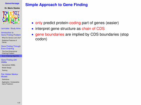
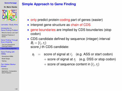
Simple Approach to Gene Finding
• only predict protein-coding part of genes (easier)
• interpret gene structure as chain of CDS• gene boundaries are implied by CDS boundaries (stop
codon)• CDS candidate defined by sequence (integer) interval
Bj = [`j , rj )score j-th CDS candidate:
sj = score of signal at `j (e.g. ASS or start codon)+ score of signal at rj (e.g. DSS or stop codon)+ score of sequence content in [`j , rj )
• use chaining algorithm to find “best” exon chain

Genvorhersage
Dr. Mario Stanke
Lernziele / Study Aims
Introduction toGene-Finding-ProblemWhat Do Genes Look Like?
Statistical Features ofGenes
Gene Finding ThroughExon-ChainingThe One-DimensionalChaining Problem
Exon-Chaining Algorithm
Gene Finding withHMMsGeneralized HMMs
Model Design
Training
Pair Hidden MarkovModelsDefinitions
Application: ComparativeGene Prediction
1.22
Simple Approach to Gene Finding
• only predict protein-coding part of genes (easier)• interpret gene structure as chain of CDS
• gene boundaries are implied by CDS boundaries (stopcodon)
• CDS candidate defined by sequence (integer) intervalBj = [`j , rj )score j-th CDS candidate:
sj = score of signal at `j (e.g. ASS or start codon)+ score of signal at rj (e.g. DSS or stop codon)+ score of sequence content in [`j , rj )
• use chaining algorithm to find “best” exon chain
Genvorhersage
Dr. Mario Stanke
Lernziele / Study Aims
Introduction toGene-Finding-ProblemWhat Do Genes Look Like?
Statistical Features ofGenes
Gene Finding ThroughExon-ChainingThe One-DimensionalChaining Problem
Exon-Chaining Algorithm
Gene Finding withHMMsGeneralized HMMs
Model Design
Training
Pair Hidden MarkovModelsDefinitions
Application: ComparativeGene Prediction
1.22
Simple Approach to Gene Finding
• only predict protein-coding part of genes (easier)• interpret gene structure as chain of CDS• gene boundaries are implied by CDS boundaries (stop
codon)
• CDS candidate defined by sequence (integer) intervalBj = [`j , rj )score j-th CDS candidate:
sj = score of signal at `j (e.g. ASS or start codon)+ score of signal at rj (e.g. DSS or stop codon)+ score of sequence content in [`j , rj )
• use chaining algorithm to find “best” exon chain
Genvorhersage
Dr. Mario Stanke
Lernziele / Study Aims
Introduction toGene-Finding-ProblemWhat Do Genes Look Like?
Statistical Features ofGenes
Gene Finding ThroughExon-ChainingThe One-DimensionalChaining Problem
Exon-Chaining Algorithm
Gene Finding withHMMsGeneralized HMMs
Model Design
Training
Pair Hidden MarkovModelsDefinitions
Application: ComparativeGene Prediction
1.22
Simple Approach to Gene Finding
• only predict protein-coding part of genes (easier)• interpret gene structure as chain of CDS• gene boundaries are implied by CDS boundaries (stop
codon)• CDS candidate defined by sequence (integer) interval
Bj = [`j , rj )score j-th CDS candidate:
sj = score of signal at `j (e.g. ASS or start codon)+ score of signal at rj (e.g. DSS or stop codon)+ score of sequence content in [`j , rj )
• use chaining algorithm to find “best” exon chain

Genvorhersage
Dr. Mario Stanke
Lernziele / Study Aims
Introduction toGene-Finding-ProblemWhat Do Genes Look Like?
Statistical Features ofGenes
Gene Finding ThroughExon-ChainingThe One-DimensionalChaining Problem
Exon-Chaining Algorithm
Gene Finding withHMMsGeneralized HMMs
Model Design
Training
Pair Hidden MarkovModelsDefinitions
Application: ComparativeGene Prediction
1.22
Simple Approach to Gene Finding
• only predict protein-coding part of genes (easier)• interpret gene structure as chain of CDS• gene boundaries are implied by CDS boundaries (stop
codon)• CDS candidate defined by sequence (integer) interval
Bj = [`j , rj )score j-th CDS candidate:
sj = score of signal at `j (e.g. ASS or start codon)+ score of signal at rj (e.g. DSS or stop codon)+ score of sequence content in [`j , rj )
• use chaining algorithm to find “best” exon chain
Genvorhersage
Dr. Mario Stanke
Lernziele / Study Aims
Introduction toGene-Finding-ProblemWhat Do Genes Look Like?
Statistical Features ofGenes
Gene Finding ThroughExon-ChainingThe One-DimensionalChaining Problem
Exon-Chaining Algorithm
Gene Finding withHMMsGeneralized HMMs
Model Design
Training
Pair Hidden MarkovModelsDefinitions
Application: ComparativeGene Prediction
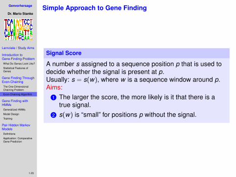
1.23
Simple Approach to Gene Finding
Signal Score
A number s assigned to a sequence position p that is used todecide whether the signal is present at p.Usually: s = s(w), where w is a sequence window around p.Aims:
1 The larger the score, the more likely is it that there is atrue signal.
2 s(w) is “small” for positions p without the signal.
Genvorhersage
Dr. Mario Stanke
Lernziele / Study Aims
Introduction toGene-Finding-ProblemWhat Do Genes Look Like?
Statistical Features ofGenes
Gene Finding ThroughExon-ChainingThe One-DimensionalChaining Problem
Exon-Chaining Algorithm
Gene Finding withHMMsGeneralized HMMs
Model Design
Training
Pair Hidden MarkovModelsDefinitions
Application: ComparativeGene Prediction
1.24
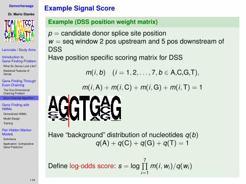
Example Signal Score
Example (DSS position weight matrix)
p = candidate donor splice site positionw = seq window 2 pos upstream and 5 pos downstream ofDSSHave position specific scoring matrix for DSS
m(i ,b) (i = 1,2, . . . ,7,b ∈ A,C,G,T),
m(i ,A) + m(i ,C) + m(i ,G) + m(i ,T) = 1
Have “background” distribution of nucleotides q(b)q(A) + q(C) + q(G) + q(T) = 1
Define log-odds score: s = log7∏
i=1m(i ,wi )/q(wi )
Genvorhersage
Dr. Mario Stanke
Lernziele / Study Aims
Introduction toGene-Finding-ProblemWhat Do Genes Look Like?
Statistical Features ofGenes
Gene Finding ThroughExon-ChainingThe One-DimensionalChaining Problem
Exon-Chaining Algorithm
Gene Finding withHMMsGeneralized HMMs
Model Design
Training
Pair Hidden MarkovModelsDefinitions
Application: ComparativeGene Prediction
1.25
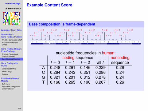
Example Content Score
Base composition is frame-dependent
f = 0f = 1
f = 2
f = 0f = 1
f = 2
f = 0f = 1
f = 2
f = 0f = 1
f = 2
f = 0f = 1
f = 2
f = 0f = 1
f = 2
f = 0f = 1
f = 2
f = 0f = 1
f = 2
nucleotide frequencies in human:coding sequence noncoding
f = 0 f = 1 f = 2 all f sequenceA 0.248 0.291 0.146 0.229 0.26C 0.264 0.243 0.351 0.286 0.24G 0.321 0.201 0.312 0.278 0.24T 0.166 0.265 0.190 0.207 0.26
Genvorhersage
Dr. Mario Stanke
Lernziele / Study Aims
Introduction toGene-Finding-ProblemWhat Do Genes Look Like?
Statistical Features ofGenes
Gene Finding ThroughExon-ChainingThe One-DimensionalChaining Problem
Exon-Chaining Algorithm
Gene Finding withHMMsGeneralized HMMs
Model Design
Training
Pair Hidden MarkovModelsDefinitions
Application: ComparativeGene Prediction
1.26
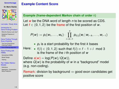
Example Content Score
Example (frame-dependent Markov chain of order k )
Let w be the DNA word of length n to be scored as CDS.Let f ∈ {0,1,2} be the frame of the first position of w .
P(w) := pf (w1, . . . ,wk ) ·n∏
i=k+1
pf (i)(wi |wi−k , . . . ,wi−1)
Here:• pf is a start probability for the first k bases• f (i) ∈ {0,1,2} such that f (i) ≡ f − 1 + i mod 3
is the frame of the i-th position of w
Define s(w) = log(P(w)/Q(w)),where Q(w) is the probability of w in a “background” model(e.g. non-coding).
Remark: division by background⇒ good exon candidates getpositive score
Genvorhersage
Dr. Mario Stanke
Lernziele / Study Aims
Introduction toGene-Finding-ProblemWhat Do Genes Look Like?
Statistical Features ofGenes
Gene Finding ThroughExon-ChainingThe One-DimensionalChaining Problem
Exon-Chaining Algorithm
Gene Finding withHMMsGeneralized HMMs
Model Design
Training
Pair Hidden MarkovModelsDefinitions
Application: ComparativeGene Prediction
1.27
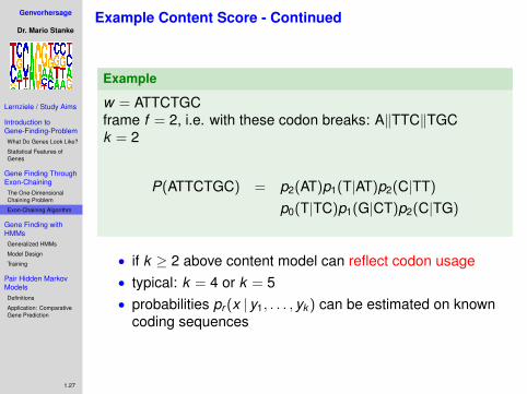
Example Content Score - Continued
Example
w = ATTCTGCframe f = 2, i.e. with these codon breaks: A‖TTC‖TGCk = 2
P(ATTCTGC) = p2(AT)p1(T|AT)p2(C|TT)
p0(T|TC)p1(G|CT)p2(C|TG)
• if k ≥ 2 above content model can reflect codon usage• typical: k = 4 or k = 5• probabilities pr (x | y1, . . . , yk ) can be estimated on known
coding sequences

Genvorhersage
Dr. Mario Stanke
Lernziele / Study Aims
Introduction toGene-Finding-ProblemWhat Do Genes Look Like?
Statistical Features ofGenes
Gene Finding ThroughExon-ChainingThe One-DimensionalChaining Problem
Exon-Chaining Algorithm
Gene Finding withHMMsGeneralized HMMs
Model Design
Training
Pair Hidden MarkovModelsDefinitions
Application: ComparativeGene Prediction
1.28
Problems with Simple Approach
• reading frame consistency not enforced
• ⇒ output can be biologically “senseless”• ⇒ less accurate when this info is ignored• CDS candidates with negative score are never used
Need extension to chaining algorithm to enforce consistency.
Genvorhersage
Dr. Mario Stanke
Lernziele / Study Aims
Introduction toGene-Finding-ProblemWhat Do Genes Look Like?
Statistical Features ofGenes
Gene Finding ThroughExon-ChainingThe One-DimensionalChaining Problem
Exon-Chaining Algorithm
Gene Finding withHMMsGeneralized HMMs
Model Design
Training
Pair Hidden MarkovModelsDefinitions
Application: ComparativeGene Prediction
1.28
Problems with Simple Approach
• reading frame consistency not enforced• ⇒ output can be biologically “senseless”
• ⇒ less accurate when this info is ignored• CDS candidates with negative score are never used
Need extension to chaining algorithm to enforce consistency.
Genvorhersage
Dr. Mario Stanke
Lernziele / Study Aims
Introduction toGene-Finding-ProblemWhat Do Genes Look Like?
Statistical Features ofGenes
Gene Finding ThroughExon-ChainingThe One-DimensionalChaining Problem
Exon-Chaining Algorithm
Gene Finding withHMMsGeneralized HMMs
Model Design
Training
Pair Hidden MarkovModelsDefinitions
Application: ComparativeGene Prediction
1.28
Problems with Simple Approach
• reading frame consistency not enforced• ⇒ output can be biologically “senseless”• ⇒ less accurate when this info is ignored
• CDS candidates with negative score are never used
Need extension to chaining algorithm to enforce consistency.

Genvorhersage
Dr. Mario Stanke
Lernziele / Study Aims
Introduction toGene-Finding-ProblemWhat Do Genes Look Like?
Statistical Features ofGenes
Gene Finding ThroughExon-ChainingThe One-DimensionalChaining Problem
Exon-Chaining Algorithm
Gene Finding withHMMsGeneralized HMMs
Model Design
Training
Pair Hidden MarkovModelsDefinitions
Application: ComparativeGene Prediction
1.28
Problems with Simple Approach
• reading frame consistency not enforced• ⇒ output can be biologically “senseless”• ⇒ less accurate when this info is ignored• CDS candidates with negative score are never used
Need extension to chaining algorithm to enforce consistency.
Genvorhersage
Dr. Mario Stanke
Lernziele / Study Aims
Introduction toGene-Finding-ProblemWhat Do Genes Look Like?
Statistical Features ofGenes
Gene Finding ThroughExon-ChainingThe One-DimensionalChaining Problem
Exon-Chaining Algorithm
Gene Finding withHMMsGeneralized HMMs
Model Design
Training
Pair Hidden MarkovModelsDefinitions
Application: ComparativeGene Prediction
1.29
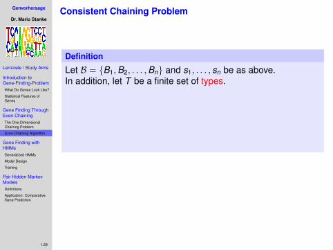
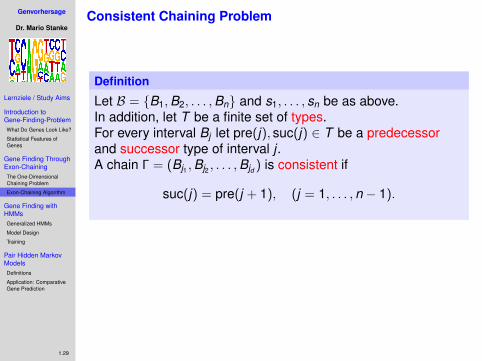
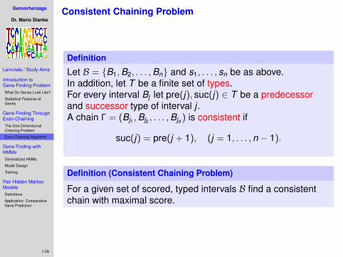
Consistent Chaining Problem
Definition
Let B = {B1,B2, . . . ,Bn} and s1, . . . , sn be as above.In addition, let T be a finite set of types.
For every interval Bj let pre(j), suc(j) ∈ T be a predecessorand successor type of interval j .A chain Γ = (Bj1 ,Bj2 , . . . ,Bjd ) is consistent if
suc(j) = pre(j + 1), (j = 1, . . . ,n − 1).
Definition (Consistent Chaining Problem)
For a given set of scored, typed intervals B find a consistentchain with maximal score.

Genvorhersage
Dr. Mario Stanke
Lernziele / Study Aims
Introduction toGene-Finding-ProblemWhat Do Genes Look Like?
Statistical Features ofGenes
Gene Finding ThroughExon-ChainingThe One-DimensionalChaining Problem
Exon-Chaining Algorithm
Gene Finding withHMMsGeneralized HMMs
Model Design
Training
Pair Hidden MarkovModelsDefinitions
Application: ComparativeGene Prediction
1.29
Consistent Chaining Problem
Definition
Let B = {B1,B2, . . . ,Bn} and s1, . . . , sn be as above.In addition, let T be a finite set of types.For every interval Bj let pre(j), suc(j) ∈ T be a predecessorand successor type of interval j .
A chain Γ = (Bj1 ,Bj2 , . . . ,Bjd ) is consistent if
suc(j) = pre(j + 1), (j = 1, . . . ,n − 1).
Definition (Consistent Chaining Problem)
For a given set of scored, typed intervals B find a consistentchain with maximal score.
Genvorhersage
Dr. Mario Stanke
Lernziele / Study Aims
Introduction toGene-Finding-ProblemWhat Do Genes Look Like?
Statistical Features ofGenes
Gene Finding ThroughExon-ChainingThe One-DimensionalChaining Problem
Exon-Chaining Algorithm
Gene Finding withHMMsGeneralized HMMs
Model Design
Training
Pair Hidden MarkovModelsDefinitions
Application: ComparativeGene Prediction
1.29
Consistent Chaining Problem
Definition
Let B = {B1,B2, . . . ,Bn} and s1, . . . , sn be as above.In addition, let T be a finite set of types.For every interval Bj let pre(j), suc(j) ∈ T be a predecessorand successor type of interval j .A chain Γ = (Bj1 ,Bj2 , . . . ,Bjd ) is consistent if
suc(j) = pre(j + 1), (j = 1, . . . ,n − 1).
Definition (Consistent Chaining Problem)
For a given set of scored, typed intervals B find a consistentchain with maximal score.
Genvorhersage
Dr. Mario Stanke
Lernziele / Study Aims
Introduction toGene-Finding-ProblemWhat Do Genes Look Like?
Statistical Features ofGenes
Gene Finding ThroughExon-ChainingThe One-DimensionalChaining Problem
Exon-Chaining Algorithm
Gene Finding withHMMsGeneralized HMMs
Model Design
Training
Pair Hidden MarkovModelsDefinitions
Application: ComparativeGene Prediction
1.30
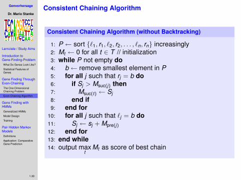
Consistent Chaining Algorithm
Consistent Chaining Algorithm (without Backtracking)
1: P ← sort {`1, r1, `2, r2, . . . , `n, rn} increasingly2: Mt ← 0 for all t ∈ T // initialization3: while P not empty do4: b ← remove smallest element in P5: for all j such that rj = b do6: if Sj > Msuc(j) then7: Msuc(t) ← Sj8: end if9: end for
10: for all j such that `j = b do11: Sj ← sj + Mpre(j)12: end for13: end while14: output max
tMt as score of best chain
Genvorhersage
Dr. Mario Stanke
Lernziele / Study Aims
Introduction toGene-Finding-ProblemWhat Do Genes Look Like?
Statistical Features ofGenes
Gene Finding ThroughExon-ChainingThe One-DimensionalChaining Problem
Exon-Chaining Algorithm
Gene Finding withHMMsGeneralized HMMs
Model Design
Training
Pair Hidden MarkovModelsDefinitions
Application: ComparativeGene Prediction
1.31
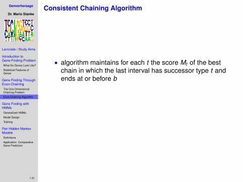
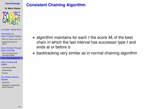
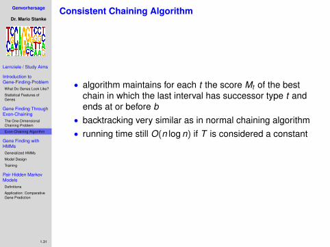
Consistent Chaining Algorithm
• algorithm maintains for each t the score Mt of the bestchain in which the last interval has successor type t andends at or before b
• backtracking very similar as in normal chaining algorithm• running time still O(n log n) if T is considered a constant• best chain can now include intervals with negative score
Genvorhersage
Dr. Mario Stanke
Lernziele / Study Aims
Introduction toGene-Finding-ProblemWhat Do Genes Look Like?
Statistical Features ofGenes
Gene Finding ThroughExon-ChainingThe One-DimensionalChaining Problem
Exon-Chaining Algorithm
Gene Finding withHMMsGeneralized HMMs
Model Design
Training
Pair Hidden MarkovModelsDefinitions
Application: ComparativeGene Prediction
1.31
Consistent Chaining Algorithm
• algorithm maintains for each t the score Mt of the bestchain in which the last interval has successor type t andends at or before b
• backtracking very similar as in normal chaining algorithm
• running time still O(n log n) if T is considered a constant• best chain can now include intervals with negative score
Genvorhersage
Dr. Mario Stanke
Lernziele / Study Aims
Introduction toGene-Finding-ProblemWhat Do Genes Look Like?
Statistical Features ofGenes
Gene Finding ThroughExon-ChainingThe One-DimensionalChaining Problem
Exon-Chaining Algorithm
Gene Finding withHMMsGeneralized HMMs
Model Design
Training
Pair Hidden MarkovModelsDefinitions
Application: ComparativeGene Prediction
1.31
Consistent Chaining Algorithm
• algorithm maintains for each t the score Mt of the bestchain in which the last interval has successor type t andends at or before b
• backtracking very similar as in normal chaining algorithm• running time still O(n log n) if T is considered a constant
• best chain can now include intervals with negative score
Genvorhersage
Dr. Mario Stanke
Lernziele / Study Aims
Introduction toGene-Finding-ProblemWhat Do Genes Look Like?
Statistical Features ofGenes
Gene Finding ThroughExon-ChainingThe One-DimensionalChaining Problem
Exon-Chaining Algorithm
Gene Finding withHMMsGeneralized HMMs
Model Design
Training
Pair Hidden MarkovModelsDefinitions
Application: ComparativeGene Prediction
1.31
Consistent Chaining Algorithm
• algorithm maintains for each t the score Mt of the bestchain in which the last interval has successor type t andends at or before b
• backtracking very similar as in normal chaining algorithm• running time still O(n log n) if T is considered a constant• best chain can now include intervals with negative score
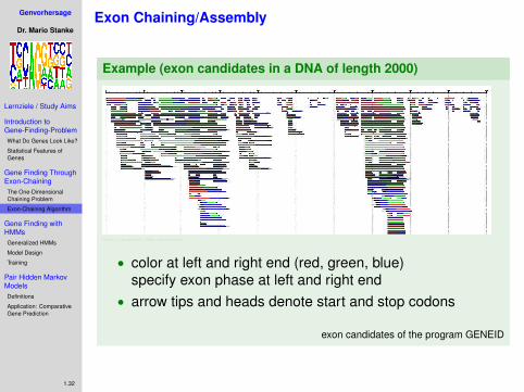
Genvorhersage
Dr. Mario Stanke
Lernziele / Study Aims
Introduction toGene-Finding-ProblemWhat Do Genes Look Like?
Statistical Features ofGenes
Gene Finding ThroughExon-ChainingThe One-DimensionalChaining Problem
Exon-Chaining Algorithm
Gene Finding withHMMsGeneralized HMMs
Model Design
Training
Pair Hidden MarkovModelsDefinitions
Application: ComparativeGene Prediction
1.32
Exon Chaining/Assembly
Example (exon candidates in a DNA of length 2000)
http://monstre1.imim.es/courses
• color at left and right end (red, green, blue)specify exon phase at left and right end
• arrow tips and heads denote start and stop codons
exon candidates of the program GENEID
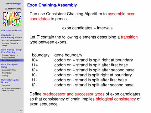
Genvorhersage
Dr. Mario Stanke
Lernziele / Study Aims
Introduction toGene-Finding-ProblemWhat Do Genes Look Like?
Statistical Features ofGenes
Gene Finding ThroughExon-ChainingThe One-DimensionalChaining Problem
Exon-Chaining Algorithm
Gene Finding withHMMsGeneralized HMMs
Model Design
Training
Pair Hidden MarkovModelsDefinitions
Application: ComparativeGene Prediction
1.33
Exon Chaining/Assembly
Can use Consistent Chaining Algorithm to assemble exoncandidates to genes.
exon candidates = intervals
Let T contain the following elements describing a transitiontype between exons.
boundary gene boundaryf0+ codon on + strand is split right at boundaryf1+ codon on + strand is split after first basef2+ codon on + strand is split after second basef0- codon on - strand is split right at boundaryf1- codon on - strand is split after first basef2- codon on - strand is split after second base
Define predecessor and successor types of exon candidatesso that consistency of chain implies biological consistency ofexon sequence.

Genvorhersage
Dr. Mario Stanke
Lernziele / Study Aims
Introduction toGene-Finding-ProblemWhat Do Genes Look Like?
Statistical Features ofGenes
Gene Finding ThroughExon-ChainingThe One-DimensionalChaining Problem
Exon-Chaining Algorithm
Gene Finding withHMMsGeneralized HMMs
Model Design
Training
Pair Hidden MarkovModelsDefinitions
Application: ComparativeGene Prediction
1.34
Consistent Exon Chain
Example
ATG *** CTA
suc(2) = f2+ = pre(3)
suc(1) = f0+ = pre(2) suc(3) = boundary = pre(4)
suc(4) = f2− = pre(5)
B B B B B3 51 2 4
***TAG* ******** * CAT**

Genvorhersage
Dr. Mario Stanke
Lernziele / Study Aims
Introduction toGene-Finding-ProblemWhat Do Genes Look Like?
Statistical Features ofGenes
Gene Finding ThroughExon-ChainingThe One-DimensionalChaining Problem
Exon-Chaining Algorithm
Gene Finding withHMMsGeneralized HMMs
Model Design
Training
Pair Hidden MarkovModelsDefinitions
Application: ComparativeGene Prediction
1.35
Issues of the Exon Chaining Approach
Problematic:
• introns are not modelled at all:• no length distribution considered• no difference to intergenic region
• UTRs: How can one accomodate for exons like these?UTR CDS
• dividing by background probability implicitly assumes thatthere are only two alternatives, e.g. exon↔ noncodingbut there are more than two alternatives for a region
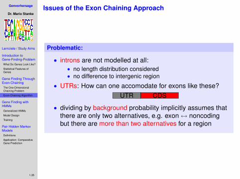
Genvorhersage
Dr. Mario Stanke
Lernziele / Study Aims
Introduction toGene-Finding-ProblemWhat Do Genes Look Like?
Statistical Features ofGenes
Gene Finding ThroughExon-ChainingThe One-DimensionalChaining Problem
Exon-Chaining Algorithm
Gene Finding withHMMsGeneralized HMMs
Model Design
Training
Pair Hidden MarkovModelsDefinitions
Application: ComparativeGene Prediction
1.36
1 Introduction to Gene-Finding-ProblemWhat Do Genes Look Like?Statistical Features of Genes
2 Gene Finding Through Exon-ChainingThe One-Dimensional Chaining ProblemExon-Chaining Algorithm
3 Gene Finding with HMMsGeneralized HMMsModel DesignTraining
4 Pair Hidden Markov ModelsDefinitionsApplication: Comparative Gene Prediction

Genvorhersage
Dr. Mario Stanke
Lernziele / Study Aims
Introduction toGene-Finding-ProblemWhat Do Genes Look Like?
Statistical Features ofGenes
Gene Finding ThroughExon-ChainingThe One-DimensionalChaining Problem
Exon-Chaining Algorithm
Gene Finding withHMMsGeneralized HMMs
Model Design
Training
Pair Hidden MarkovModelsDefinitions
Application: ComparativeGene Prediction
1.37
Reminder: Hidden Markov Model
HMM
• A HMM is a probabilistic model of a wordy = y1y2 · · · yn (“emission”) over some alphabet Σ and of astate sequence x = (x1, x2, · · · , xn) over some discrete setof states Q.
• The joint distribution of x and y is of the form
P(x , y) =n∏
i=1
p(xi |xi−1) · p(yi |xi ),
where the p(xi |xi−1) are the transition probabilities of aMarkov chain and the p(yi |xi ) are alled emissionprobabilities.
(x0 is a start state to simplify notation)
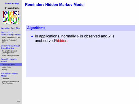
Genvorhersage
Dr. Mario Stanke
Lernziele / Study Aims
Introduction toGene-Finding-ProblemWhat Do Genes Look Like?
Statistical Features ofGenes
Gene Finding ThroughExon-ChainingThe One-DimensionalChaining Problem
Exon-Chaining Algorithm
Gene Finding withHMMsGeneralized HMMs
Model Design
Training
Pair Hidden MarkovModelsDefinitions
Application: ComparativeGene Prediction
1.38
Reminder: Hidden Markov Model
Algorithms
• In applications, normally y is observed and x isunobserved/hidden.
• The Viterbi algorithm computes a most likely statesequence x̂ ∈ arg maxx P(x |y) in time O(n).
• The Forward algorithm can be used to compute P(x , y) intime O(n).
• The Forward and Backward algorithms can be used tocompute posterior probabilities P(xi = q|y) in time O(n).
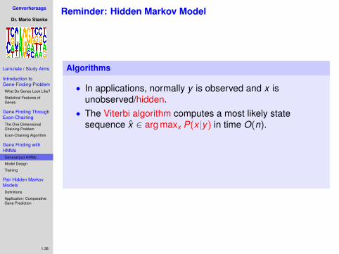
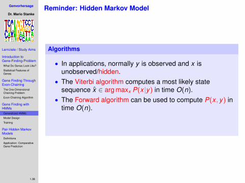
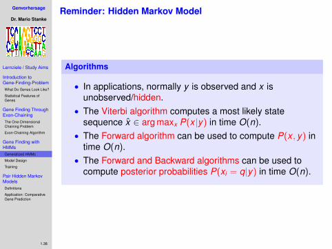

Genvorhersage
Dr. Mario Stanke
Lernziele / Study Aims
Introduction toGene-Finding-ProblemWhat Do Genes Look Like?
Statistical Features ofGenes
Gene Finding ThroughExon-ChainingThe One-DimensionalChaining Problem
Exon-Chaining Algorithm
Gene Finding withHMMsGeneralized HMMs
Model Design
Training
Pair Hidden MarkovModelsDefinitions
Application: ComparativeGene Prediction
1.39
Reminder: Generalized Hidden Markov Model
Why GHMMs?
• A HMM is a special case of a GHMM.
• In gene finding and for alignment tasksGHMMs are often used because
1 they allow a detailed modelling of the length distribution ofexons and other biological intervals
2 they accomodate for “silent” or “delete” states required tomodel alignment gaps
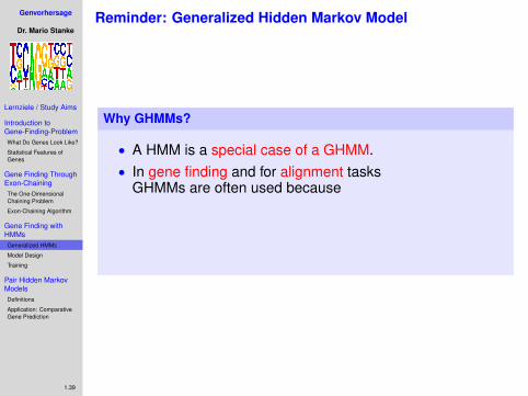
Genvorhersage
Dr. Mario Stanke
Lernziele / Study Aims
Introduction toGene-Finding-ProblemWhat Do Genes Look Like?
Statistical Features ofGenes
Gene Finding ThroughExon-ChainingThe One-DimensionalChaining Problem
Exon-Chaining Algorithm
Gene Finding withHMMsGeneralized HMMs
Model Design
Training
Pair Hidden MarkovModelsDefinitions
Application: ComparativeGene Prediction
1.39
Reminder: Generalized Hidden Markov Model
Why GHMMs?
• A HMM is a special case of a GHMM.• In gene finding and for alignment tasks
GHMMs are often used because
1 they allow a detailed modelling of the length distribution ofexons and other biological intervals
2 they accomodate for “silent” or “delete” states required tomodel alignment gaps

Genvorhersage
Dr. Mario Stanke
Lernziele / Study Aims
Introduction toGene-Finding-ProblemWhat Do Genes Look Like?
Statistical Features ofGenes
Gene Finding ThroughExon-ChainingThe One-DimensionalChaining Problem
Exon-Chaining Algorithm
Gene Finding withHMMsGeneralized HMMs
Model Design
Training
Pair Hidden MarkovModelsDefinitions
Application: ComparativeGene Prediction
1.39
Reminder: Generalized Hidden Markov Model
Why GHMMs?
• A HMM is a special case of a GHMM.• In gene finding and for alignment tasks
GHMMs are often used because1 they allow a detailed modelling of the length distribution of
exons and other biological intervals
2 they accomodate for “silent” or “delete” states required tomodel alignment gaps
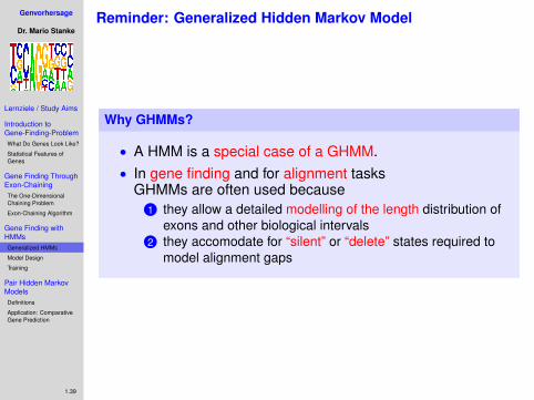
Genvorhersage
Dr. Mario Stanke
Lernziele / Study Aims
Introduction toGene-Finding-ProblemWhat Do Genes Look Like?
Statistical Features ofGenes
Gene Finding ThroughExon-ChainingThe One-DimensionalChaining Problem
Exon-Chaining Algorithm
Gene Finding withHMMsGeneralized HMMs
Model Design
Training
Pair Hidden MarkovModelsDefinitions
Application: ComparativeGene Prediction
1.39
Reminder: Generalized Hidden Markov Model
Why GHMMs?
• A HMM is a special case of a GHMM.• In gene finding and for alignment tasks
GHMMs are often used because1 they allow a detailed modelling of the length distribution of
exons and other biological intervals2 they accomodate for “silent” or “delete” states required to
model alignment gaps
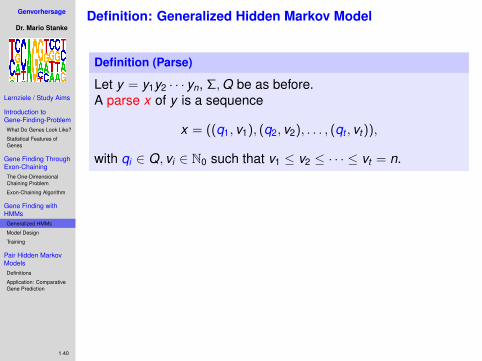
Genvorhersage
Dr. Mario Stanke
Lernziele / Study Aims
Introduction toGene-Finding-ProblemWhat Do Genes Look Like?
Statistical Features ofGenes
Gene Finding ThroughExon-ChainingThe One-DimensionalChaining Problem
Exon-Chaining Algorithm
Gene Finding withHMMsGeneralized HMMs
Model Design
Training
Pair Hidden MarkovModelsDefinitions
Application: ComparativeGene Prediction
1.40
Definition: Generalized Hidden Markov Model
Definition (Parse)
Let y = y1y2 · · · yn, Σ,Q be as before.A parse x of y is a sequence
x = ((q1, v1), (q2, v2), . . . , (qt , vt )),
with qi ∈ Q, vi ∈ N0 such that v1 ≤ v2 ≤ · · · ≤ vt = n.
2 vq
d
qv11qv = 00v
y1 y2 y3 v1y
2 ii
i−1y(v
i
vt
ny
t−1vi−1v
, v ]i
qt
• observe that y decomposes via x intoy = y(v0, v1]y(v1, v2] · · · y(vn−1, vn] (v0 := 0)
• we say that state “qi ends at vi ”• we call di := vi − vi−1 the length of the i-th emission
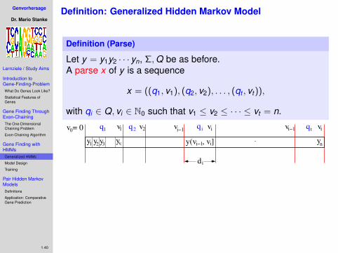
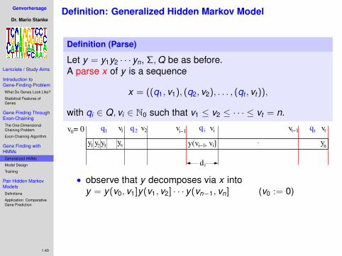
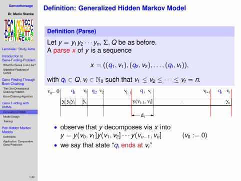
Genvorhersage
Dr. Mario Stanke
Lernziele / Study Aims
Introduction toGene-Finding-ProblemWhat Do Genes Look Like?
Statistical Features ofGenes
Gene Finding ThroughExon-ChainingThe One-DimensionalChaining Problem
Exon-Chaining Algorithm
Gene Finding withHMMsGeneralized HMMs
Model Design
Training
Pair Hidden MarkovModelsDefinitions
Application: ComparativeGene Prediction
1.40
Definition: Generalized Hidden Markov Model
Definition (Parse)
Let y = y1y2 · · · yn, Σ,Q be as before.A parse x of y is a sequence
x = ((q1, v1), (q2, v2), . . . , (qt , vt )),
with qi ∈ Q, vi ∈ N0 such that v1 ≤ v2 ≤ · · · ≤ vt = n.
2 vq
d
qv11qv = 00v
y1 y2 y3 v1y
2 ii
i−1y(v
i
vt
ny
t−1vi−1v
, v ]i
qt
• observe that y decomposes via x intoy = y(v0, v1]y(v1, v2] · · · y(vn−1, vn] (v0 := 0)
• we say that state “qi ends at vi ”
• we call di := vi − vi−1 the length of the i-th emission
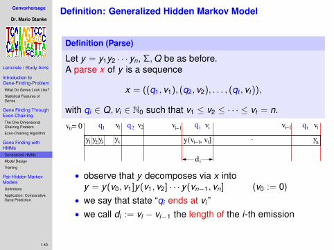
Genvorhersage
Dr. Mario Stanke
Lernziele / Study Aims
Introduction toGene-Finding-ProblemWhat Do Genes Look Like?
Statistical Features ofGenes
Gene Finding ThroughExon-ChainingThe One-DimensionalChaining Problem
Exon-Chaining Algorithm
Gene Finding withHMMsGeneralized HMMs
Model Design
Training
Pair Hidden MarkovModelsDefinitions
Application: ComparativeGene Prediction
1.40
Definition: Generalized Hidden Markov Model
Definition (Parse)
Let y = y1y2 · · · yn, Σ,Q be as before.A parse x of y is a sequence
x = ((q1, v1), (q2, v2), . . . , (qt , vt )),
with qi ∈ Q, vi ∈ N0 such that v1 ≤ v2 ≤ · · · ≤ vt = n.
2 vq
d
qv11qv = 00v
y1 y2 y3 v1y
2 ii
i−1y(v
i
vt
ny
t−1vi−1v
, v ]i
qt
• observe that y decomposes via x intoy = y(v0, v1]y(v1, v2] · · · y(vn−1, vn] (v0 := 0)
• we say that state “qi ends at vi ”• we call di := vi − vi−1 the length of the i-th emission
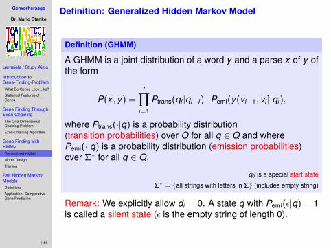
Genvorhersage
Dr. Mario Stanke
Lernziele / Study Aims
Introduction toGene-Finding-ProblemWhat Do Genes Look Like?
Statistical Features ofGenes
Gene Finding ThroughExon-ChainingThe One-DimensionalChaining Problem
Exon-Chaining Algorithm
Gene Finding withHMMsGeneralized HMMs
Model Design
Training
Pair Hidden MarkovModelsDefinitions
Application: ComparativeGene Prediction
1.41
Definition: Generalized Hidden Markov Model
Definition (GHMM)
A GHMM is a joint distribution of a word y and a parse x of y ofthe form
P(x , y) =t∏
i=1
Ptrans(qi |qi−i ) · Pemi(y(vi−1, vi ]|qi ),
where Ptrans(·|q) is a probability distribution(transition probabilities) over Q for all q ∈ Q and wherePemi(·|q) is a probability distribution (emission probabilities)over Σ∗ for all q ∈ Q.
q0 is a special start state
Σ∗ = {all strings with letters in Σ} (includes empty string)
Remark: We explicitly allow di = 0. A state q with Pemi(ε|q) = 1is called a silent state (ε is the empty string of length 0).
Genvorhersage
Dr. Mario Stanke
Lernziele / Study Aims
Introduction toGene-Finding-ProblemWhat Do Genes Look Like?
Statistical Features ofGenes
Gene Finding ThroughExon-ChainingThe One-DimensionalChaining Problem
Exon-Chaining Algorithm
Gene Finding withHMMsGeneralized HMMs
Model Design
Training
Pair Hidden MarkovModelsDefinitions
Application: ComparativeGene Prediction
1.42
Delineation of HMM
When is a GHMM called a HMM?
• A HMM is a GHMM in which di ≡ 1 for all i , i.e. allemissions are a single character. In that special case theparse x can be identified with the state sequence, whichhas the same length as y
• Sometimes in the literature a GHMM, in which di ∈ {0,1},is still called a HMM only with some special modificationsto the algorithms. Example: “delete” state in profile HMMs
Genvorhersage
Dr. Mario Stanke
Lernziele / Study Aims
Introduction toGene-Finding-ProblemWhat Do Genes Look Like?
Statistical Features ofGenes
Gene Finding ThroughExon-ChainingThe One-DimensionalChaining Problem
Exon-Chaining Algorithm
Gene Finding withHMMsGeneralized HMMs
Model Design
Training
Pair Hidden MarkovModelsDefinitions
Application: ComparativeGene Prediction
1.43
Algorithms for GHMM
Algorithms
1 Usually, the word y is observed.Now: A concatenation of the emissions, not the sequenceof emissions.Contrast to HMM: The emissions cannot be inferred fromy alone.
2 x is unobserved, neither the states nor their boundariesare known.
3 Analogous Viterbi, Forward and Backward algorithmsexists that all run in O(n2). Important special case: theyrun in O(n) if all di are bounded from above by a constant.
4 A prerequisite for points 3 above is that no loops of stateswith just empty-word-emissions are possible.We will ensure that by the design of the model topology.
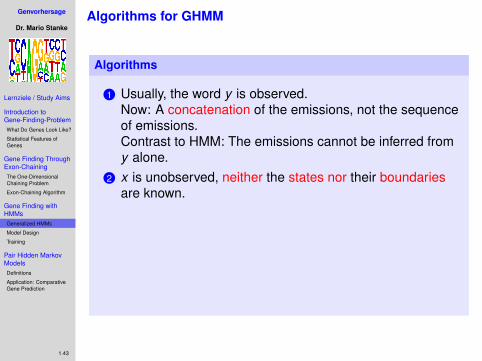
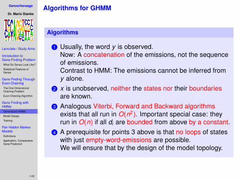
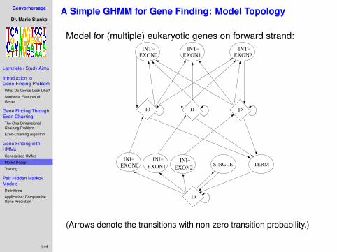
Genvorhersage
Dr. Mario Stanke
Lernziele / Study Aims
Introduction toGene-Finding-ProblemWhat Do Genes Look Like?
Statistical Features ofGenes
Gene Finding ThroughExon-ChainingThe One-DimensionalChaining Problem
Exon-Chaining Algorithm
Gene Finding withHMMsGeneralized HMMs
Model Design
Training
Pair Hidden MarkovModelsDefinitions
Application: ComparativeGene Prediction
1.44
A Simple GHMM for Gene Finding: Model Topology
Model for (multiple) eukaryotic genes on forward strand:
IR
I1 I2I0
TERMSINGLEEXON1 EXON2
EXON0
EXON0
EXON1 EXON2INT− INT−INT−
INI− INI− INI−
(Arrows denote the transitions with non-zero transition probability.)
Genvorhersage
Dr. Mario Stanke
Lernziele / Study Aims
Introduction toGene-Finding-ProblemWhat Do Genes Look Like?
Statistical Features ofGenes
Gene Finding ThroughExon-ChainingThe One-DimensionalChaining Problem
Exon-Chaining Algorithm
Gene Finding withHMMsGeneralized HMMs
Model Design
Training
Pair Hidden MarkovModelsDefinitions
Application: ComparativeGene Prediction
1.45
What (Most) Eukaryotic Species Have in Common?
In Common:
• same genetic code, including start and stop codons
• genes can have introns, may have many• genes rarely overlap in sequence• introns start almost always with GT, end with AG
(some introns GC/AG)• more non-coding sequence than coding sequence
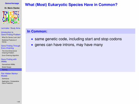
Genvorhersage
Dr. Mario Stanke
Lernziele / Study Aims
Introduction toGene-Finding-ProblemWhat Do Genes Look Like?
Statistical Features ofGenes
Gene Finding ThroughExon-ChainingThe One-DimensionalChaining Problem
Exon-Chaining Algorithm
Gene Finding withHMMsGeneralized HMMs
Model Design
Training
Pair Hidden MarkovModelsDefinitions
Application: ComparativeGene Prediction
1.45
What (Most) Eukaryotic Species Have in Common?
In Common:
• same genetic code, including start and stop codons• genes can have introns, may have many
• genes rarely overlap in sequence• introns start almost always with GT, end with AG
(some introns GC/AG)• more non-coding sequence than coding sequence
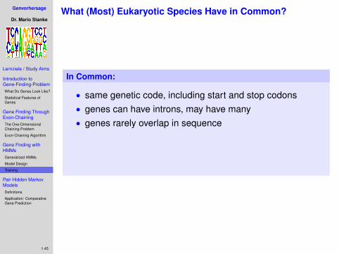
Genvorhersage
Dr. Mario Stanke
Lernziele / Study Aims
Introduction toGene-Finding-ProblemWhat Do Genes Look Like?
Statistical Features ofGenes
Gene Finding ThroughExon-ChainingThe One-DimensionalChaining Problem
Exon-Chaining Algorithm
Gene Finding withHMMsGeneralized HMMs
Model Design
Training
Pair Hidden MarkovModelsDefinitions
Application: ComparativeGene Prediction
1.45
What (Most) Eukaryotic Species Have in Common?
In Common:
• same genetic code, including start and stop codons• genes can have introns, may have many• genes rarely overlap in sequence
• introns start almost always with GT, end with AG(some introns GC/AG)
• more non-coding sequence than coding sequence

Genvorhersage
Dr. Mario Stanke
Lernziele / Study Aims
Introduction toGene-Finding-ProblemWhat Do Genes Look Like?
Statistical Features ofGenes
Gene Finding ThroughExon-ChainingThe One-DimensionalChaining Problem
Exon-Chaining Algorithm
Gene Finding withHMMsGeneralized HMMs
Model Design
Training
Pair Hidden MarkovModelsDefinitions
Application: ComparativeGene Prediction
1.45
What (Most) Eukaryotic Species Have in Common?
In Common:
• same genetic code, including start and stop codons• genes can have introns, may have many• genes rarely overlap in sequence• introns start almost always with GT, end with AG
(some introns GC/AG)
• more non-coding sequence than coding sequence

Genvorhersage
Dr. Mario Stanke
Lernziele / Study Aims
Introduction toGene-Finding-ProblemWhat Do Genes Look Like?
Statistical Features ofGenes
Gene Finding ThroughExon-ChainingThe One-DimensionalChaining Problem
Exon-Chaining Algorithm
Gene Finding withHMMsGeneralized HMMs
Model Design
Training
Pair Hidden MarkovModelsDefinitions
Application: ComparativeGene Prediction
1.45
What (Most) Eukaryotic Species Have in Common?
In Common:
• same genetic code, including start and stop codons• genes can have introns, may have many• genes rarely overlap in sequence• introns start almost always with GT, end with AG
(some introns GC/AG)• more non-coding sequence than coding sequence

Genvorhersage
Dr. Mario Stanke
Lernziele / Study Aims
Introduction toGene-Finding-ProblemWhat Do Genes Look Like?
Statistical Features ofGenes
Gene Finding ThroughExon-ChainingThe One-DimensionalChaining Problem
Exon-Chaining Algorithm
Gene Finding withHMMsGeneralized HMMs
Model Design
Training
Pair Hidden MarkovModelsDefinitions
Application: ComparativeGene Prediction
1.46
How Species-Specific Must Gene Finding Models Be?
Differences:
• distribution at signals, e.g. branch point region
top: human / bottom: fly
• GC content highly variable• number and length distribution of introns• length distribution of UTRs• gene density
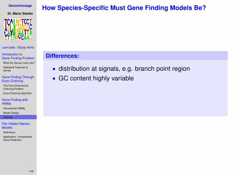
Genvorhersage
Dr. Mario Stanke
Lernziele / Study Aims
Introduction toGene-Finding-ProblemWhat Do Genes Look Like?
Statistical Features ofGenes
Gene Finding ThroughExon-ChainingThe One-DimensionalChaining Problem
Exon-Chaining Algorithm
Gene Finding withHMMsGeneralized HMMs
Model Design
Training
Pair Hidden MarkovModelsDefinitions
Application: ComparativeGene Prediction
1.46
How Species-Specific Must Gene Finding Models Be?
Differences:
• distribution at signals, e.g. branch point region• GC content highly variable
• number and length distribution of introns• length distribution of UTRs• gene density
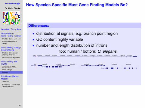
Genvorhersage
Dr. Mario Stanke
Lernziele / Study Aims
Introduction toGene-Finding-ProblemWhat Do Genes Look Like?
Statistical Features ofGenes
Gene Finding ThroughExon-ChainingThe One-DimensionalChaining Problem
Exon-Chaining Algorithm
Gene Finding withHMMsGeneralized HMMs
Model Design
Training
Pair Hidden MarkovModelsDefinitions
Application: ComparativeGene Prediction
1.46
How Species-Specific Must Gene Finding Models Be?
Differences:
• distribution at signals, e.g. branch point region• GC content highly variable• number and length distribution of introns
top: human / bottom: C. eleganschr21: 33250000 33260000 33270000 33280000 33290000 33300000 33310000 33320000 33330000 33340000 33350000 33360000 33370000HUNK
chrII: 15005000 15010000 15015000 15020000 15025000 15030000 15035000Y53F4B.10
Y53F4B.9Y53F4B.11 Y53F4B.12
Y53F4B.13
• length distribution of UTRs• gene density
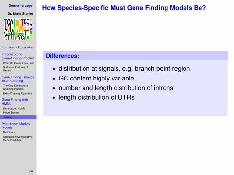
Genvorhersage
Dr. Mario Stanke
Lernziele / Study Aims
Introduction toGene-Finding-ProblemWhat Do Genes Look Like?
Statistical Features ofGenes
Gene Finding ThroughExon-ChainingThe One-DimensionalChaining Problem
Exon-Chaining Algorithm
Gene Finding withHMMsGeneralized HMMs
Model Design
Training
Pair Hidden MarkovModelsDefinitions
Application: ComparativeGene Prediction
1.46
How Species-Specific Must Gene Finding Models Be?
Differences:
• distribution at signals, e.g. branch point region• GC content highly variable• number and length distribution of introns• length distribution of UTRs
• gene density
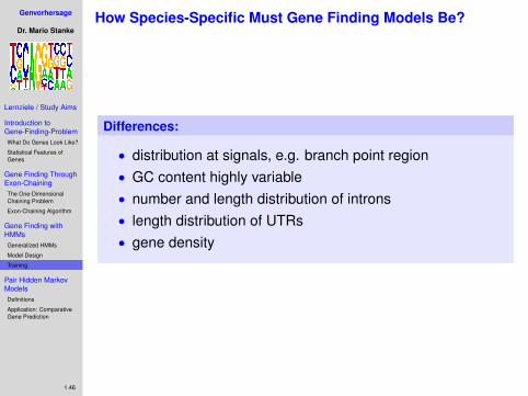
Genvorhersage
Dr. Mario Stanke
Lernziele / Study Aims
Introduction toGene-Finding-ProblemWhat Do Genes Look Like?
Statistical Features ofGenes
Gene Finding ThroughExon-ChainingThe One-DimensionalChaining Problem
Exon-Chaining Algorithm
Gene Finding withHMMsGeneralized HMMs
Model Design
Training
Pair Hidden MarkovModelsDefinitions
Application: ComparativeGene Prediction
1.46
How Species-Specific Must Gene Finding Models Be?
Differences:
• distribution at signals, e.g. branch point region• GC content highly variable• number and length distribution of introns• length distribution of UTRs• gene density
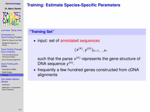
Genvorhersage
Dr. Mario Stanke
Lernziele / Study Aims
Introduction toGene-Finding-ProblemWhat Do Genes Look Like?
Statistical Features ofGenes
Gene Finding ThroughExon-ChainingThe One-DimensionalChaining Problem
Exon-Chaining Algorithm
Gene Finding withHMMsGeneralized HMMs
Model Design
Training
Pair Hidden MarkovModelsDefinitions
Application: ComparativeGene Prediction
1.47
Training: Estimate Species-Specific Parameters
“Training Set”
• input: set of annotated sequences
(x (k), y (k))k=1,...,N ,
such that the parse x (k) represents the gene structure ofDNA sequence y (k).
• frequently a few hundred genes constructed from cDNAalignments
Genvorhersage
Dr. Mario Stanke
Lernziele / Study Aims
Introduction toGene-Finding-ProblemWhat Do Genes Look Like?
Statistical Features ofGenes
Gene Finding ThroughExon-ChainingThe One-DimensionalChaining Problem
Exon-Chaining Algorithm
Gene Finding withHMMsGeneralized HMMs
Model Design
Training
Pair Hidden MarkovModelsDefinitions
Application: ComparativeGene Prediction
1.48
1 Introduction to Gene-Finding-ProblemWhat Do Genes Look Like?Statistical Features of Genes
2 Gene Finding Through Exon-ChainingThe One-Dimensional Chaining ProblemExon-Chaining Algorithm
3 Gene Finding with HMMsGeneralized HMMsModel DesignTraining
4 Pair Hidden Markov ModelsDefinitionsApplication: Comparative Gene Prediction

Genvorhersage
Dr. Mario Stanke
Lernziele / Study Aims
Introduction toGene-Finding-ProblemWhat Do Genes Look Like?
Statistical Features ofGenes
Gene Finding ThroughExon-ChainingThe One-DimensionalChaining Problem
Exon-Chaining Algorithm
Gene Finding withHMMsGeneralized HMMs
Model Design
Training
Pair Hidden MarkovModelsDefinitions
Application: ComparativeGene Prediction
1.49
Pair HMM versus standard HMM
Pair HMM
• same concept of hidden states
• two observed sequences y and z instead of just one• an association between character pairs yi and zj is usually
sought but a priori not known• typical Bioinformatics applications:
alignments, comparative gene finding
Genvorhersage
Dr. Mario Stanke
Lernziele / Study Aims
Introduction toGene-Finding-ProblemWhat Do Genes Look Like?
Statistical Features ofGenes
Gene Finding ThroughExon-ChainingThe One-DimensionalChaining Problem
Exon-Chaining Algorithm
Gene Finding withHMMsGeneralized HMMs
Model Design
Training
Pair Hidden MarkovModelsDefinitions
Application: ComparativeGene Prediction
1.49
Pair HMM versus standard HMM
Pair HMM
• same concept of hidden states• two observed sequences y and z instead of just one
• an association between character pairs yi and zj is usuallysought but a priori not known
• typical Bioinformatics applications:alignments, comparative gene finding
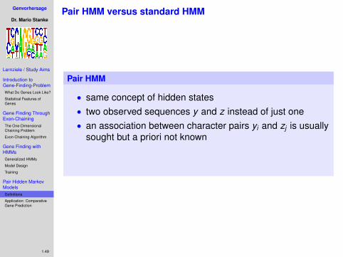
Genvorhersage
Dr. Mario Stanke
Lernziele / Study Aims
Introduction toGene-Finding-ProblemWhat Do Genes Look Like?
Statistical Features ofGenes
Gene Finding ThroughExon-ChainingThe One-DimensionalChaining Problem
Exon-Chaining Algorithm
Gene Finding withHMMsGeneralized HMMs
Model Design
Training
Pair Hidden MarkovModelsDefinitions
Application: ComparativeGene Prediction
1.49
Pair HMM versus standard HMM
Pair HMM
• same concept of hidden states• two observed sequences y and z instead of just one• an association between character pairs yi and zj is usually
sought but a priori not known
• typical Bioinformatics applications:alignments, comparative gene finding
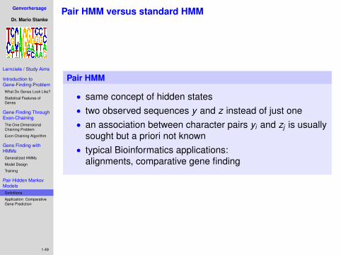
Genvorhersage
Dr. Mario Stanke
Lernziele / Study Aims
Introduction toGene-Finding-ProblemWhat Do Genes Look Like?
Statistical Features ofGenes
Gene Finding ThroughExon-ChainingThe One-DimensionalChaining Problem
Exon-Chaining Algorithm
Gene Finding withHMMsGeneralized HMMs
Model Design
Training
Pair Hidden MarkovModelsDefinitions
Application: ComparativeGene Prediction
1.49
Pair HMM versus standard HMM
Pair HMM
• same concept of hidden states• two observed sequences y and z instead of just one• an association between character pairs yi and zj is usually
sought but a priori not known• typical Bioinformatics applications:
alignments, comparative gene finding
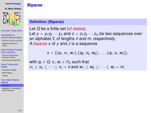
Genvorhersage
Dr. Mario Stanke
Lernziele / Study Aims
Introduction toGene-Finding-ProblemWhat Do Genes Look Like?
Statistical Features ofGenes
Gene Finding ThroughExon-ChainingThe One-DimensionalChaining Problem
Exon-Chaining Algorithm
Gene Finding withHMMsGeneralized HMMs
Model Design
Training
Pair Hidden MarkovModelsDefinitions
Application: ComparativeGene Prediction
1.50
Biparse
Definition (Biparse)
Let Q be a finite set (of states).Let y = y1y2 · · · yn and z = z1z2 · · · zm be two sequences overan alphabet Σ of lengths n and m, respectively.A biparse x of y and z is a sequence
x = ((q1, v1,w1), (q2, v2,w2), . . . , (qt , vt ,wt )),
with qi ∈ Q, vi ,wi ∈ N0 such thatv1 ≤ v2 ≤ · · · ≤ vt = n and w1 ≤ w2 ≤ · · · ≤ wt = m.
• a biparse segments 2 sequences into the same number ofsegments
• each segment pair y(vi−1, vi ], z(wi−1,wi ] corresponds asingle state qi
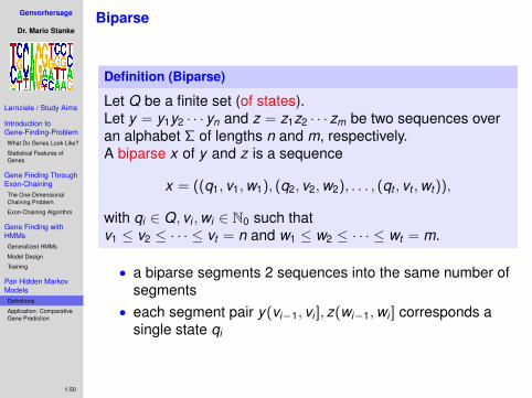
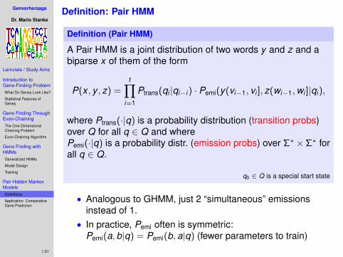
Genvorhersage
Dr. Mario Stanke
Lernziele / Study Aims
Introduction toGene-Finding-ProblemWhat Do Genes Look Like?
Statistical Features ofGenes
Gene Finding ThroughExon-ChainingThe One-DimensionalChaining Problem
Exon-Chaining Algorithm
Gene Finding withHMMsGeneralized HMMs
Model Design
Training
Pair Hidden MarkovModelsDefinitions
Application: ComparativeGene Prediction
1.51
Definition: Pair HMM
Definition (Pair HMM)
A Pair HMM is a joint distribution of two words y and z and abiparse x of them of the form
P(x , y , z) =t∏
i=1
Ptrans(qi |qi−i ) · Pemi(y(vi−1, vi ], z(wi−1,wi ]|qi ),
where Ptrans(·|q) is a probability distribution (transition probs)over Q for all q ∈ Q and wherePemi(·|q) is a probability distr. (emission probs) over Σ∗ ×Σ∗ forall q ∈ Q.
q0 ∈ Q is a special start state
• Analogous to GHMM, just 2 “simultaneous” emissionsinstead of 1.
• In practice, Pemi often is symmetric:Pemi(a,b|q) = Pemi(b,a|q) (fewer parameters to train)
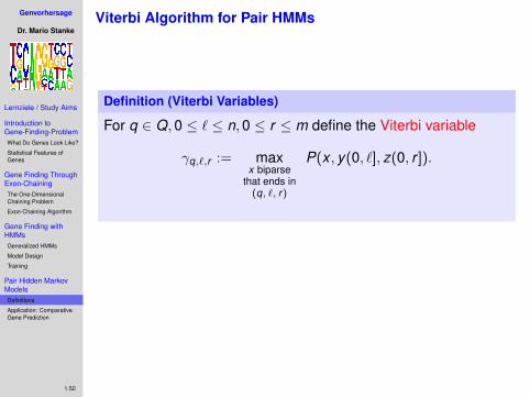
Genvorhersage
Dr. Mario Stanke
Lernziele / Study Aims
Introduction toGene-Finding-ProblemWhat Do Genes Look Like?
Statistical Features ofGenes
Gene Finding ThroughExon-ChainingThe One-DimensionalChaining Problem
Exon-Chaining Algorithm
Gene Finding withHMMsGeneralized HMMs
Model Design
Training
Pair Hidden MarkovModelsDefinitions
Application: ComparativeGene Prediction
1.52
Viterbi Algorithm for Pair HMMs
Definition (Viterbi Variables)
For q ∈ Q,0 ≤ ` ≤ n,0 ≤ r ≤ m define the Viterbi variable
γq,`,r := maxx biparse
that ends in(q, `, r)
P(x , y(0, `], z(0, r ]).
Interpretation
γq,`,r is the probability of the most likely parseof y up to ` and of z up to r that ends in state q.
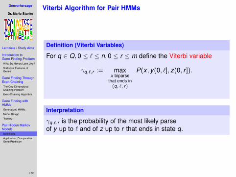
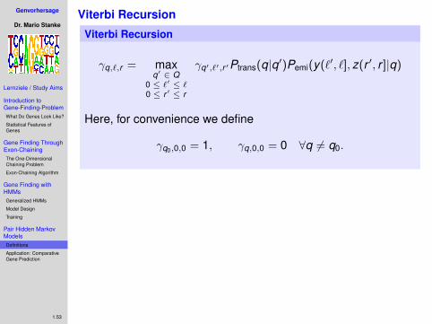
Genvorhersage
Dr. Mario Stanke
Lernziele / Study Aims
Introduction toGene-Finding-ProblemWhat Do Genes Look Like?
Statistical Features ofGenes
Gene Finding ThroughExon-ChainingThe One-DimensionalChaining Problem
Exon-Chaining Algorithm
Gene Finding withHMMsGeneralized HMMs
Model Design
Training
Pair Hidden MarkovModelsDefinitions
Application: ComparativeGene Prediction
1.53
Viterbi Recursion
Viterbi Recursion
γq,`,r = maxq′ ∈ Q
0 ≤ `′ ≤ `0 ≤ r ′ ≤ r
γq′,`′,r ′Ptrans(q|q′)Pemi(y(`′, `], z(r ′, r ]|q)
Here, for convenience we define
γq0,0,0 = 1, γq,0,0 = 0 ∀q 6= q0.
Assumption
Never the empty string is emitted simultaneously in bothsequences:
Pemi(ε, ε|q) = 0 ∀q ∈ Q
• is anyway the case in our applications• is sufficient condition that the Viterbi recursion can be
iteratively computed
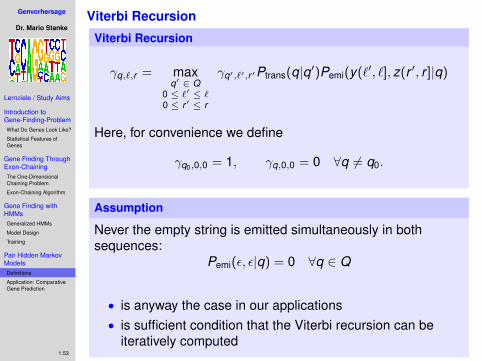
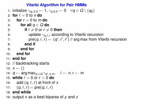
Viterbi Algorithm for Pair HMMs1: initialize γq0,0,0 ← 1, γq,0,0 ← 0 ∀q ∈ Q \ {q0}2: for ` = 0 to n do3: for r = 0 to m do4: for all q ∈ Q do5: if ` 6= 0 or r 6= 0 then6: update γq,`,r according to Viterbi recursion7: pre(q, `, r)← (q′, `′, r ′) // arg max from Viterbi recursion8: end if9: end for
10: end for11: end for12: // backtracking starts13: x ← ()14: q ← arg maxq′∈Q γq′,n,m, `← n, r ← m15: while ` > 0 or r > 0 do16: add (q, `, r) at front of x17: (q, `, r) = pre(q, `, r)18: end while19: output x as a best biparse of y and z

Running Time
• in general:
O(n2m2)
• if emissions are bounded by d :Pemi (w ,w ′|q) = 0, ∀w ,w ′ ∈ Σ∗ : |w | > d or |w ′| > d ,∀q ∈ Qwe can shortcut recursion:
γq,`,r = maxq′ ∈ Q
max{0, `− d} ≤ `′ ≤ `max{0, `− d} ≤ r ′ ≤ r
γq′,`′,r ′Ptrans(q|q′)Pemi(y(`′, `], z(`′, `]|q)
then running time is O(d2nm)
• very important special case d = 1: running time = O(nm)
• further heuristics to reduce running time possible:compute Viterbi recursion only for subset of (`, r) ∈ (0,n]× (0,m],assume it vanishes elsewhere
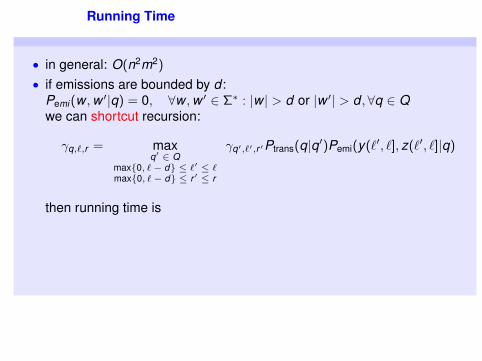
Running Time
• in general: O(n2m2)
• if emissions are bounded by d :Pemi (w ,w ′|q) = 0, ∀w ,w ′ ∈ Σ∗ : |w | > d or |w ′| > d ,∀q ∈ Qwe can shortcut recursion:
γq,`,r = maxq′ ∈ Q
max{0, `− d} ≤ `′ ≤ `max{0, `− d} ≤ r ′ ≤ r
γq′,`′,r ′Ptrans(q|q′)Pemi(y(`′, `], z(`′, `]|q)
then running time is
O(d2nm)
• very important special case d = 1: running time = O(nm)
• further heuristics to reduce running time possible:compute Viterbi recursion only for subset of (`, r) ∈ (0,n]× (0,m],assume it vanishes elsewhere
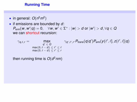
Running Time
• in general: O(n2m2)
• if emissions are bounded by d :Pemi (w ,w ′|q) = 0, ∀w ,w ′ ∈ Σ∗ : |w | > d or |w ′| > d ,∀q ∈ Qwe can shortcut recursion:
γq,`,r = maxq′ ∈ Q
max{0, `− d} ≤ `′ ≤ `max{0, `− d} ≤ r ′ ≤ r
γq′,`′,r ′Ptrans(q|q′)Pemi(y(`′, `], z(`′, `]|q)
then running time is O(d2nm)
• very important special case d = 1: running time = O(nm)
• further heuristics to reduce running time possible:compute Viterbi recursion only for subset of (`, r) ∈ (0,n]× (0,m],assume it vanishes elsewhere
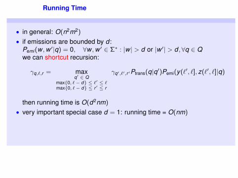
Running Time
• in general: O(n2m2)
• if emissions are bounded by d :Pemi (w ,w ′|q) = 0, ∀w ,w ′ ∈ Σ∗ : |w | > d or |w ′| > d ,∀q ∈ Qwe can shortcut recursion:
γq,`,r = maxq′ ∈ Q
max{0, `− d} ≤ `′ ≤ `max{0, `− d} ≤ r ′ ≤ r
γq′,`′,r ′Ptrans(q|q′)Pemi(y(`′, `], z(`′, `]|q)
then running time is O(d2nm)
• very important special case d = 1: running time = O(nm)
• further heuristics to reduce running time possible:compute Viterbi recursion only for subset of (`, r) ∈ (0,n]× (0,m],assume it vanishes elsewhere
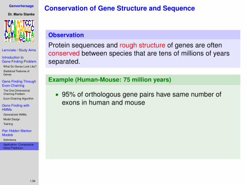
Genvorhersage
Dr. Mario Stanke
Lernziele / Study Aims
Introduction toGene-Finding-ProblemWhat Do Genes Look Like?
Statistical Features ofGenes
Gene Finding ThroughExon-ChainingThe One-DimensionalChaining Problem
Exon-Chaining Algorithm
Gene Finding withHMMsGeneralized HMMs
Model Design
Training
Pair Hidden MarkovModelsDefinitions
Application: ComparativeGene Prediction
1.56
Conservation of Gene Structure and Sequence
Observation
Protein sequences and rough structure of genes are oftenconserved between species that are tens of millions of yearsseparated.
Example (Human-Mouse: 75 million years)
• 95% of orthologous gene pairs have same number ofexons in human and mouse
• coding sequence to ≈ 85% identical--->
GapsHumanMouse
GCAC T T T T C T T A A AGGA A AGT A A TGGACC A GTGA AGGTGTGGGGA AGCA T T A A AGGAC T G AC TGA AGGCC TGCA TGGA T T CC A TGT T CA T GAGT T TGGAGA T A A T ACAGCAGGTGGGTG TE S N G P V K V W G S I K G L T E G L H G F H V H E F G D N T A GSOD1
4GCAC T T T T C T T A A AGGA A AGT A A TGGACC A GTGA AGGTGTGGGGA AGCA T T A A AGGAC T G AC TGA AGGCC TGCA TGGA T T CC A TGT T CA T GAGT T TGGAGA T A A T ACAGCAGGTGGGTG TGT A T T T T T - A T CA AGGCA AGCGGTGA ACC A GT TGTGT TGT CAGGACA A A T T ACAGGA T T A AC TGA AGGCCAGCA TGGGT T CC ACGT CCA T C AGT A TGGGGACA A T ACACA AGGT AGGT C C
• noncoding sequence to ≈ 35% identicalchr21:
--->
GapsHumanMouse
33035890 33035900 33035910 33035920 33035930 33035940 33035950 33035960 33035970 33035980 33035990AGTGTGGGA ACA AGA T T ACCA T C T CCC T T T TGAGGACACAGGCC T AGAGCAGT T A AGCA GC T TGC TGGAGGT T CAC TGGC T AGA A AGTGG T CAGCC TGGGA T T TGGAC ACAGA T T T T T C C
SOD14 3 3 6
AGTGTGGGA AC A AGA T T ACCA T C T CCC T T T TGAGGACACAGGCC T AGAGCAGT T A AGCA GC T TGC TGGAGGT T CAC TGGC T AGA A AGTGG T CAGCC TGGGA T T TGGACACAGA T T T T T C CAGTGT T AGGAGA A - - - - GTG - - - - - - - - - T GGGAGAGAGAGGCC T - - - AGAGC TGAGCG T - - - - C T CC AGAGCCAC - - - CC TGT AGGA A G T GGGT C T AGGA T C TGA AC A T AGG T T T T T T T
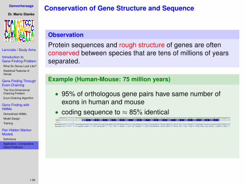
Genvorhersage
Dr. Mario Stanke
Lernziele / Study Aims
Introduction toGene-Finding-ProblemWhat Do Genes Look Like?
Statistical Features ofGenes
Gene Finding ThroughExon-ChainingThe One-DimensionalChaining Problem
Exon-Chaining Algorithm
Gene Finding withHMMsGeneralized HMMs
Model Design
Training
Pair Hidden MarkovModelsDefinitions
Application: ComparativeGene Prediction
1.56
Conservation of Gene Structure and Sequence
Observation
Protein sequences and rough structure of genes are oftenconserved between species that are tens of millions of yearsseparated.
Example (Human-Mouse: 75 million years)
• 95% of orthologous gene pairs have same number ofexons in human and mouse
• coding sequence to ≈ 85% identical--->
GapsHumanMouse
GCAC T T T T C T T A A AGGA A AGT A A TGGACC A GTGA AGGTGTGGGGA AGCA T T A A AGGAC T G AC TGA AGGCC TGCA TGGA T T CCA TGT T CA T GAGT T TGGAGA T A A T ACAGCAGGTGGGTG TE S N G P V K V W G S I K G L T E G L H G F H V H E F G D N T A GSOD1
4GCAC T T T T C T T A A AGGA A AGT A A TGGACC A GTGA AGGTGTGGGGA AGCA T T A A AGGAC T G AC TGA AGGCC TGCA TGGA T T CCA TGT T CA T GAGT T TGGAGA T A A T ACAGCAGGTGGGTG TGT A T T T T T - A T CA AGGCA AGCGGTGA ACC A GT TGTGT TGT CAGGACA A A T T ACAGGA T T A AC TGA AGGCCAGCA TGGGT T CCACGT CCA T C AGT A TGGGGACA A T ACACA AGGT AGGT C C
• noncoding sequence to ≈ 35% identicalchr21:
--->
GapsHumanMouse
33035890 33035900 33035910 33035920 33035930 33035940 33035950 33035960 33035970 33035980 33035990AGTGTGGGA ACA AGA T T ACCA T C T CCC T T T TGAGGACACAGGCC T AGAGCAGT T A AGCA GC T TGC TGGAGGT T CAC TGGC T AGA A AGTGG T CAGCC TGGGA T T TGGACACAGA T T T T T C C
SOD14 3 3 6
AGTGTGGGA ACA AGA T T ACCA T C T CCC T T T TGAGGACACAGGCC T AGAGCAGT T A AGCA GC T TGC TGGAGGT T CAC TGGC T AGA A AGTGG T CAGCC TGGGA T T TGGACACAGA T T T T T C CAGTGT T AGGAGA A - - - - GTG - - - - - - - - - T GGGAGAGAGAGGCC T - - - AGAGC TGAGCG T - - - - C T CC AGAGCCAC - - - CC TGT AGGA A G T GGGT C T AGGA T C TGA ACA T AGG T T T T T T T
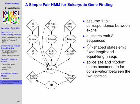
Genvorhersage
Dr. Mario Stanke
Lernziele / Study Aims
Introduction toGene-Finding-ProblemWhat Do Genes Look Like?
Statistical Features ofGenes
Gene Finding ThroughExon-ChainingThe One-DimensionalChaining Problem
Exon-Chaining Algorithm
Gene Finding withHMMsGeneralized HMMs
Model Design
Training
Pair Hidden MarkovModelsDefinitions
Application: ComparativeGene Prediction
1.57
A Simple Pair HMM for Eukaryotic Gene Finding
Start−kodon
Stopp−kodon
IR
Intron0 Intron1 Intron2
Kodons
z1gty1gt
gtgt
agag
agy3agz3
agy2y3agz2z3
z1z2gty1y2gt
• assume 1-to-1correspondence betweenexons
• all states emit 2sequences
• -shaped states emitfixed-length andequal-length seqs
• splice site and “Kodon”states accomodate forconservation between thetwo species