lecture linear filters edge detection · cos 429: computer vison linear filters and edge detection...
TRANSCRIPT

COS 429: COMPUTER VISONLinear Filters and Edge Detection
• convolution• shift invariant linear system• Fourier Transform• Aliasing and sampling• scale representation• edge detection
Reading: Chapters 7, 8


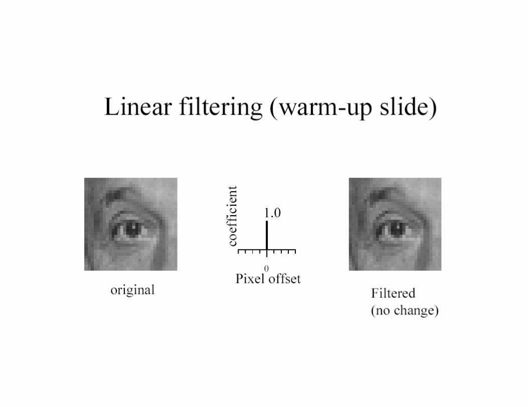
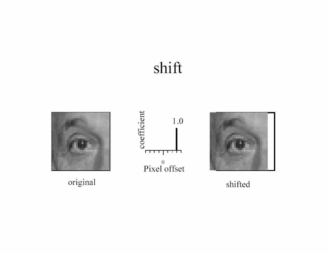
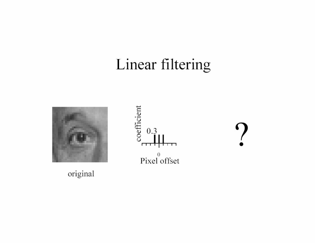
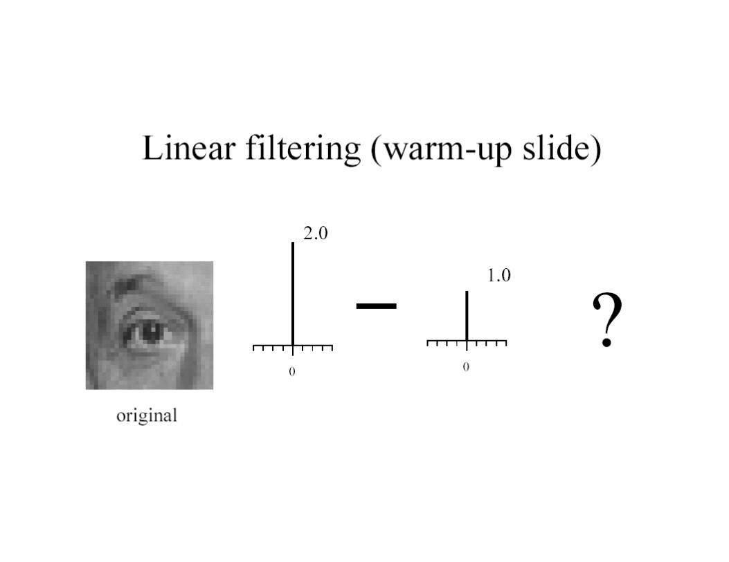
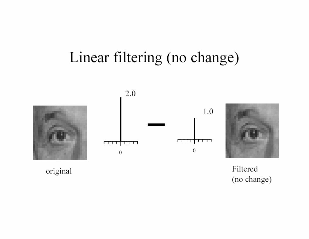
Linear Filters
• Linear filtering:– Form a new image whose pixels are a
weighted sum of original pixel values, using the same set of weights at each point

Convolution
• Represent the linear weights as an image, F
• F is called the kernel• Operation is called
convolution– Center origin of the kernel
F at each pixel location– Multiply weights by
corresponding pixels– Set resulting value for each
pixel
• Image, R, resulting from convolution of F with image H, where u,v range over kernel pixels:
Rij = Hi−u, j−vFuvu,v∑
Warning: the textbook mixes upH and F
111
111
111
Slide credit: David Lowe (UBC)

Slide credits for these examples: Bill Freeman, David Jacobs


Convolution
1/9.(10x1 + 11x1 + 10x1 + 9x1 + 10x1 + 11x1 + 10x1 + 9x1 + 10x1)1/9.(10x1 + 11x1 + 10x1 + 9x1 + 10x1 + 11x1 + 10x1 + 9x1 + 10x1) = = 1/9.( 90) = 101/9.( 90) = 10
1010 1111 101099 1010 1111
1010 99 101011
10101010
2299
0099
00
9999
9999
00
11
99991010
1010 1111
110011
11111111
1111111110101010
II
111111
1111 11
1111
11
FF
XX XX XX
XX 1010
XX
XX
XXXX
XX
XX
XX
XX
XX
XXXX
XX
XXXXXXXX
1/91/9
OO
Slide credit: Christopher Rasmussen
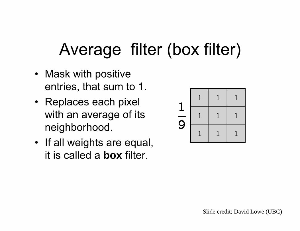
Average filter (box filter)• Mask with positive
entries, that sum to 1.• Replaces each pixel
with an average of its neighborhood.
• If all weights are equal, it is called a box filter.
111
111
111
Slide credit: David Lowe (UBC)

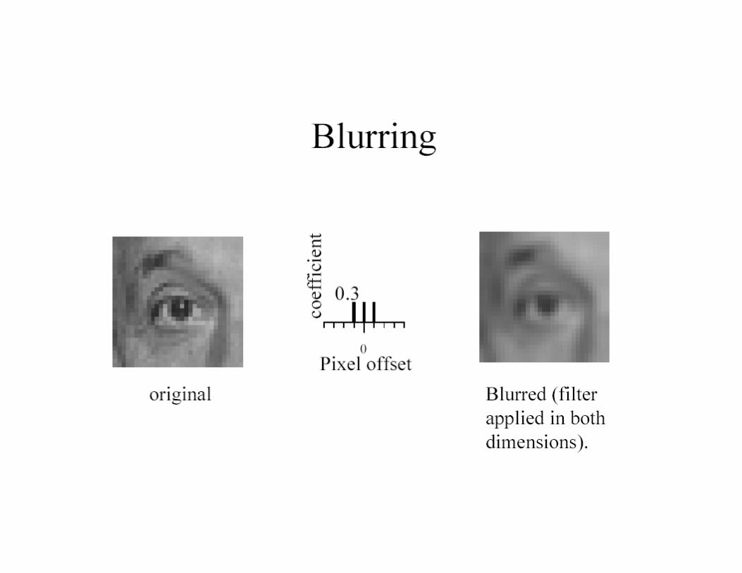
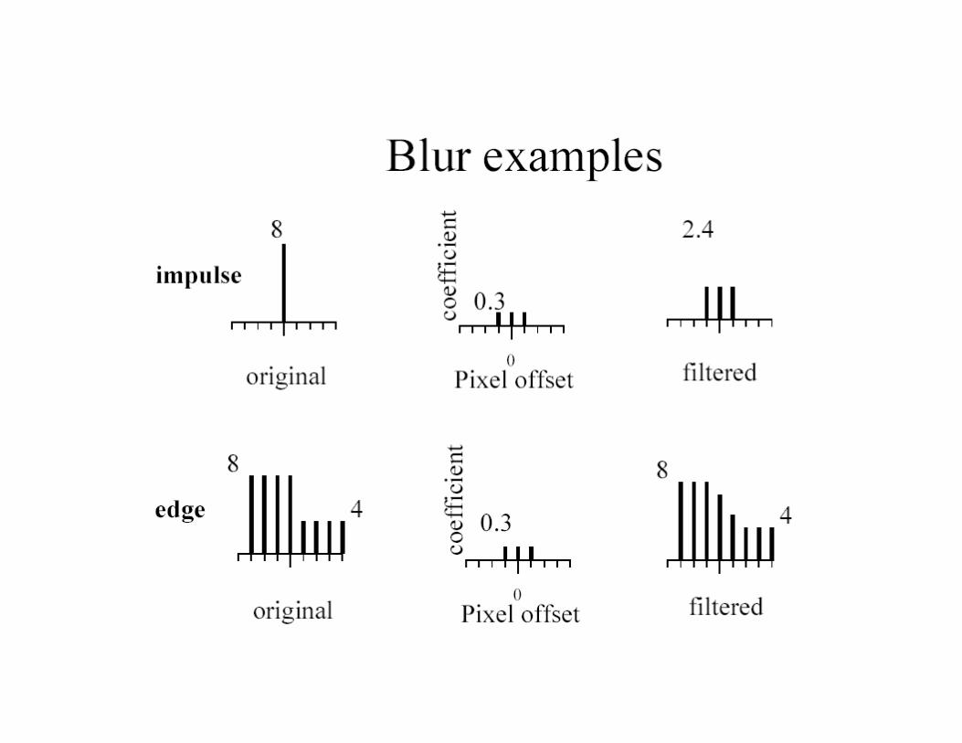
Example: Smoothing with a box filter
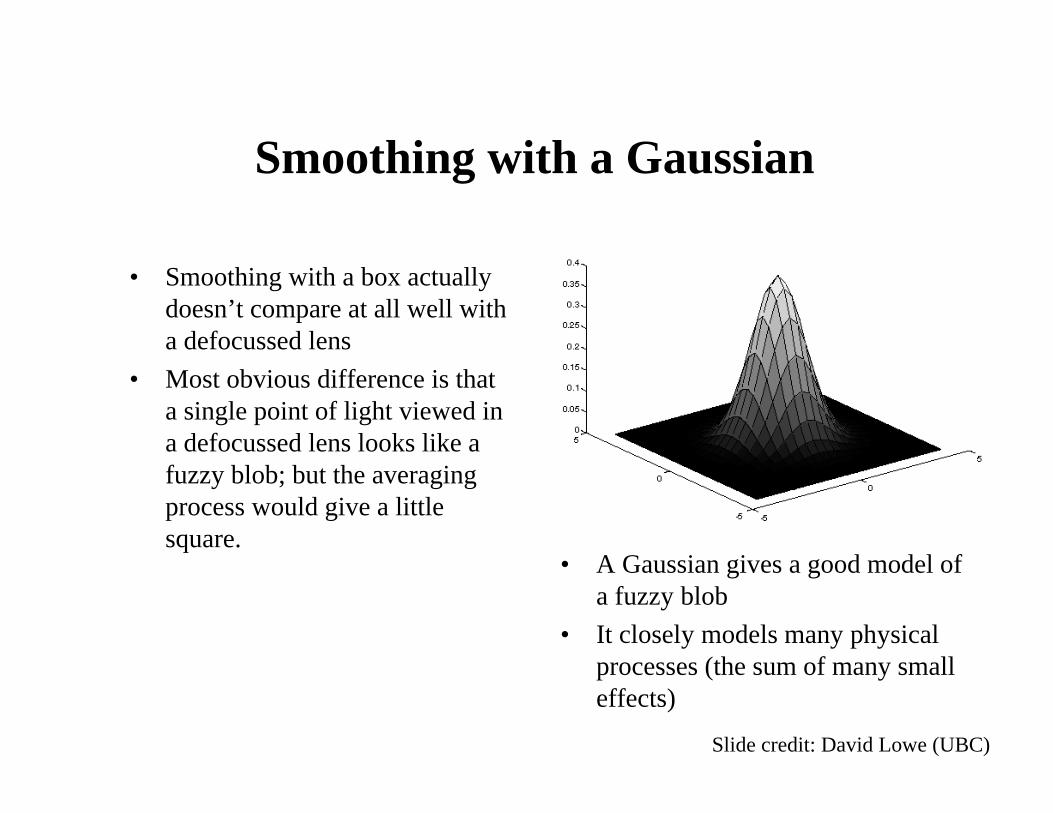
Smoothing with a Gaussian
• Smoothing with a box actually doesn’t compare at all well with a defocussed lens
• Most obvious difference is that a single point of light viewed in a defocussed lens looks like a fuzzy blob; but the averaging process would give a little square.
• A Gaussian gives a good model of a fuzzy blob
• It closely models many physical processes (the sum of many small effects)
Slide credit: David Lowe (UBC)

Gaussian Kernel• Idea: Weight contributions of neighboring pixels by nearness
• Constant factor at front makes volume sum to 1 (can be ignored, as we should normalize weights to sum to 1 in any case).
0.003 0.013 0.022 0.013 0.0030.013 0.059 0.097 0.059 0.0130.022 0.097 0.159 0.097 0.0220.013 0.059 0.097 0.059 0.0130.003 0.013 0.022 0.013 0.003
5 x 5, σ = 1
Slide credit: Christopher Rasmussen

Smoothing with a Gaussian
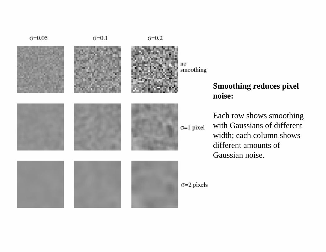
Smoothing reduces pixel noise:
Each row shows smoothingwith Gaussians of differentwidth; each column showsdifferent amounts of Gaussian noise.

Efficient Implementation
• Both the BOX filter and the Gaussian filter are separable into two 1D convolutions:– First convolve each row with a 1D filter– Then convolve each column with a 1D filter.
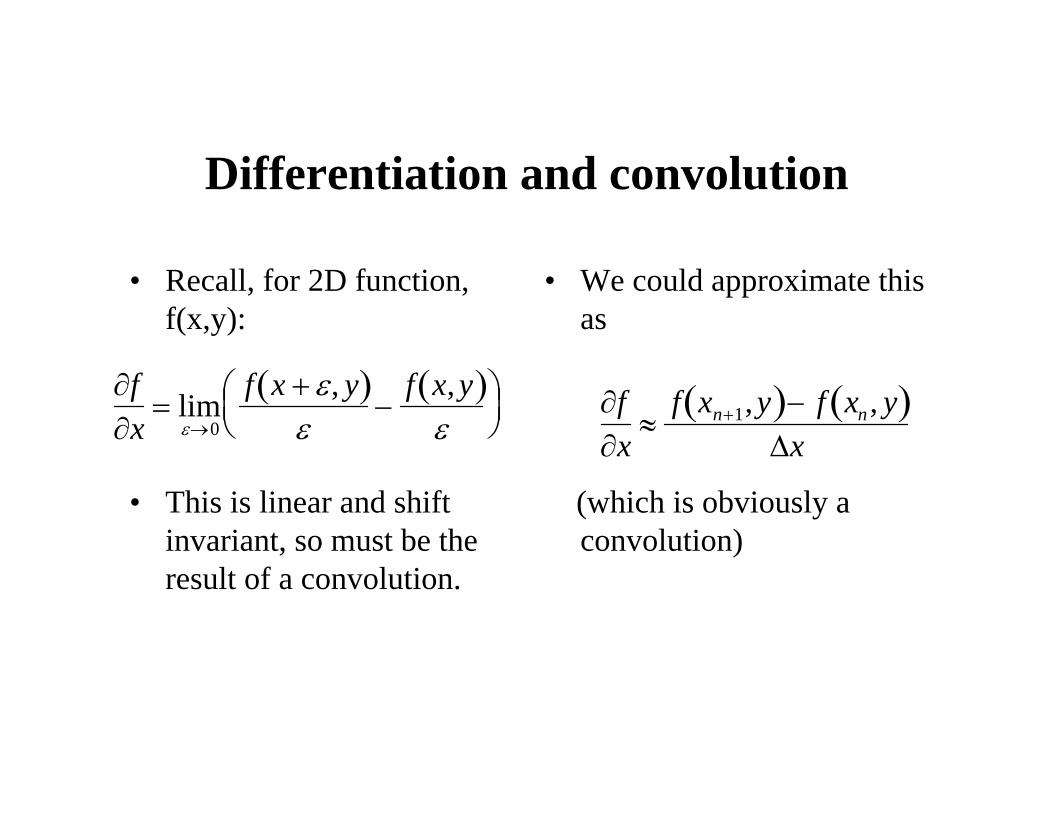
Differentiation and convolution
• Recall, for 2D function, f(x,y):
• This is linear and shift invariant, so must be the result of a convolution.
• We could approximate this as
(which is obviously a convolution)
∂f∂x
= limε→0
f x + ε, y( )ε
−f x,y( )
ε⎛ ⎝ ⎜
⎞ ⎠ ⎟ ∂f
∂x≈
f xn+1,y( )− f xn , y( )Δx

Vertical gradients from finite differences

Shift invariant linear systems
• 3 properties– Superposition– Scaling– Shift invariance
Discrete convolution
• 1D• 2D• “edge effects” in discrete convolution
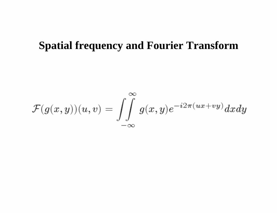
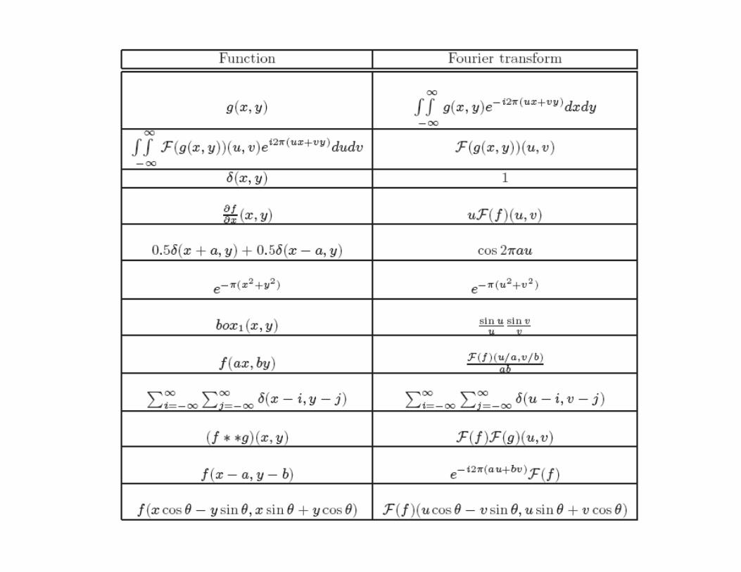
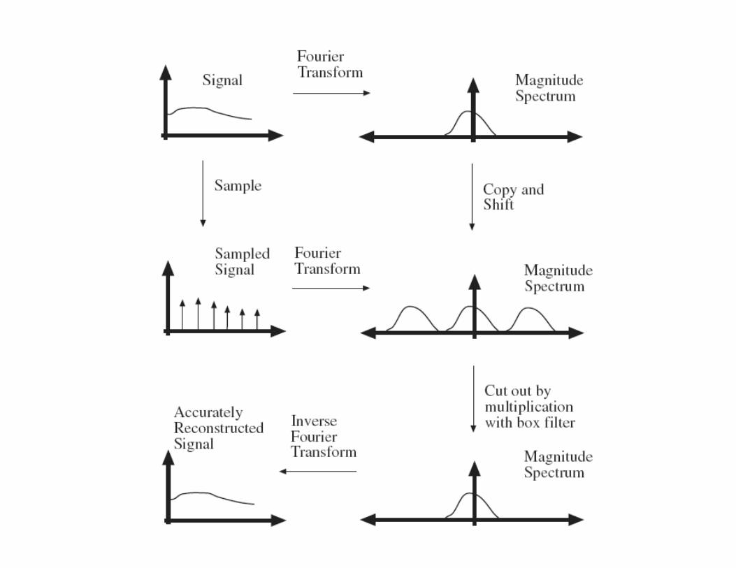
Spatial frequency and Fourier Transform
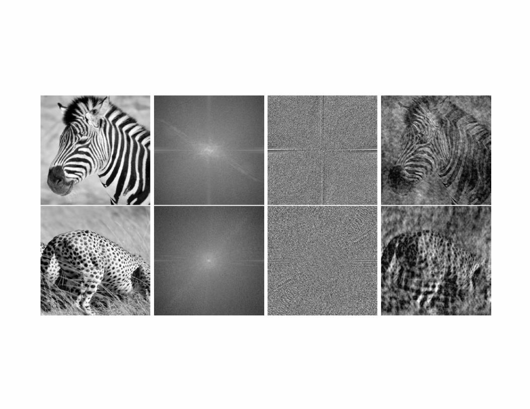
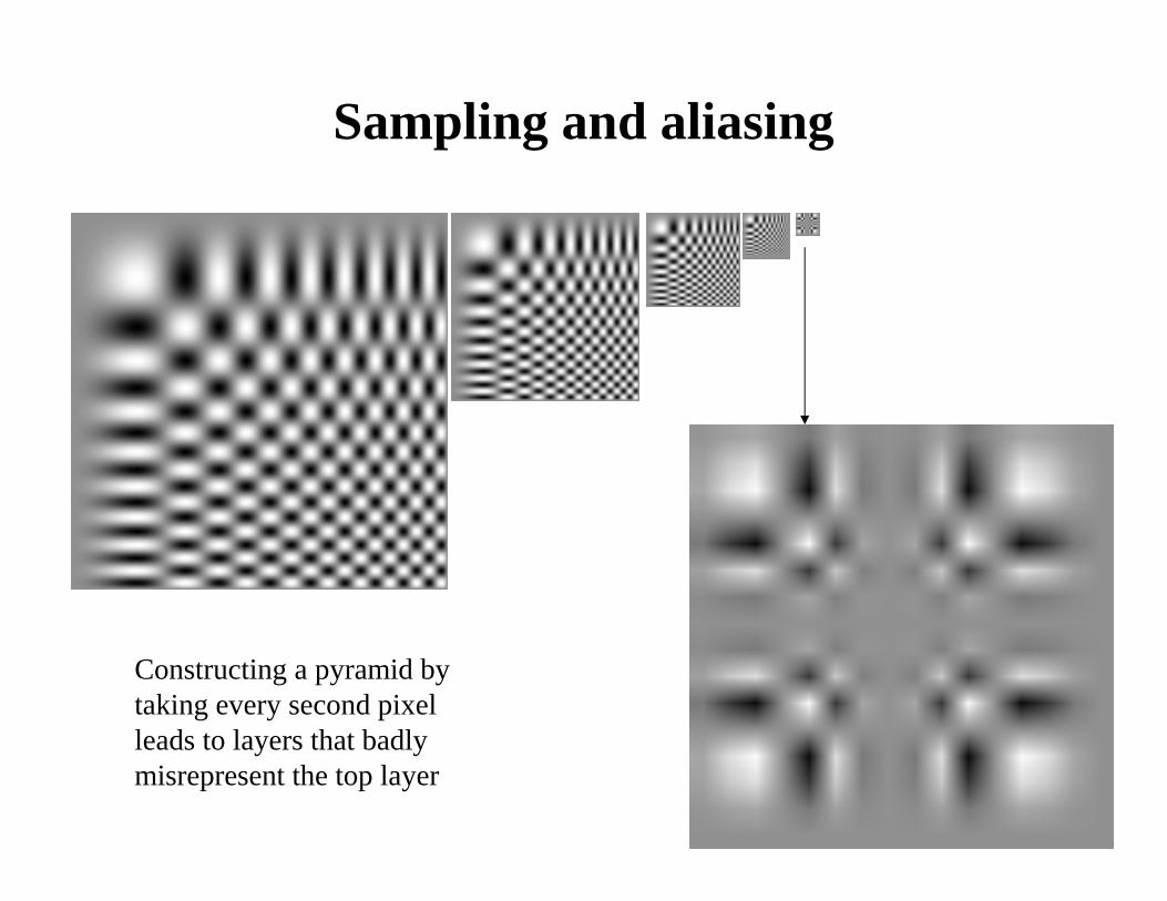
Sampling and aliasing
Constructing a pyramid by taking every second pixel leads to layers that badly misrepresent the top layer
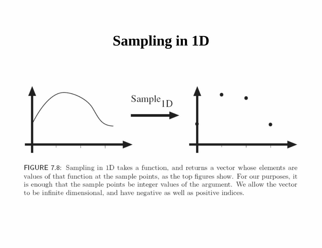
Sampling in 1D
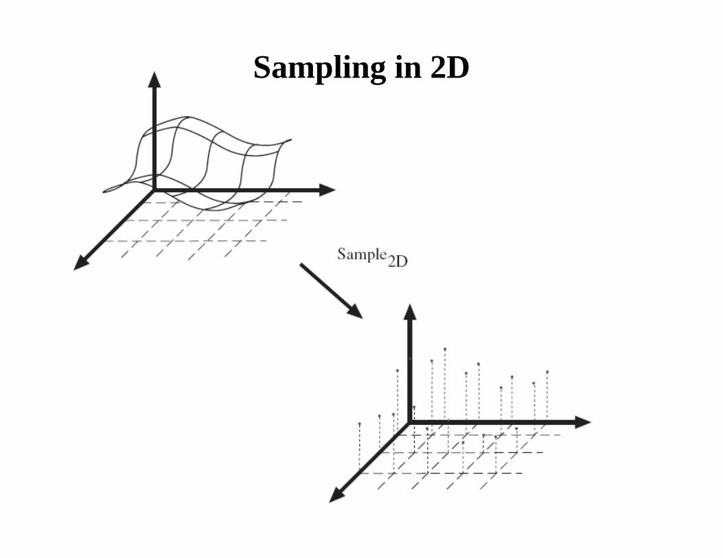
Sampling in 2D

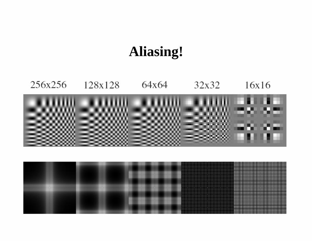
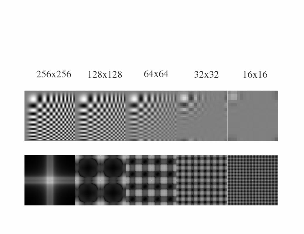
Aliasing!

Smoothing and resampling
• Nyquist’s theorem
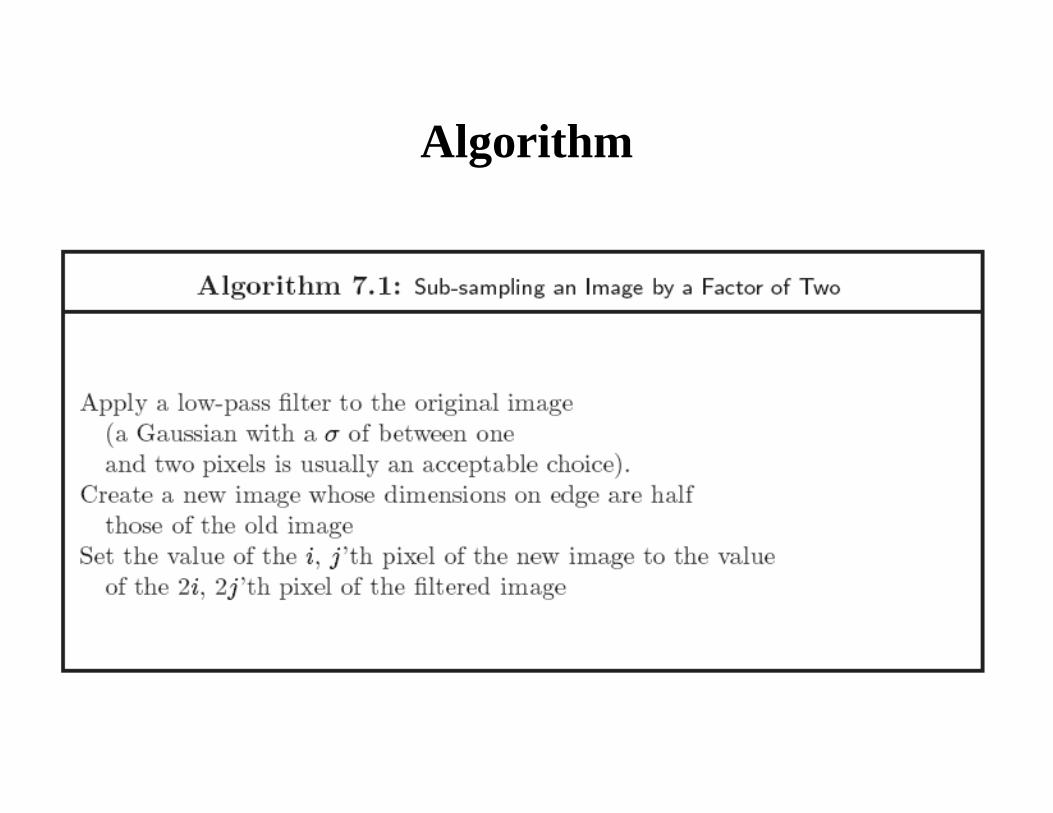
Algorithm

Filters are templates
• Applying a filter at some point can be seen as taking a dot-product between the image and some vector
• Filtering the image is a set of dot products
• Insight – filters look like the effects
they are intended to find– filters find effects they look
like
Slide credit: David Lowe (UBC)
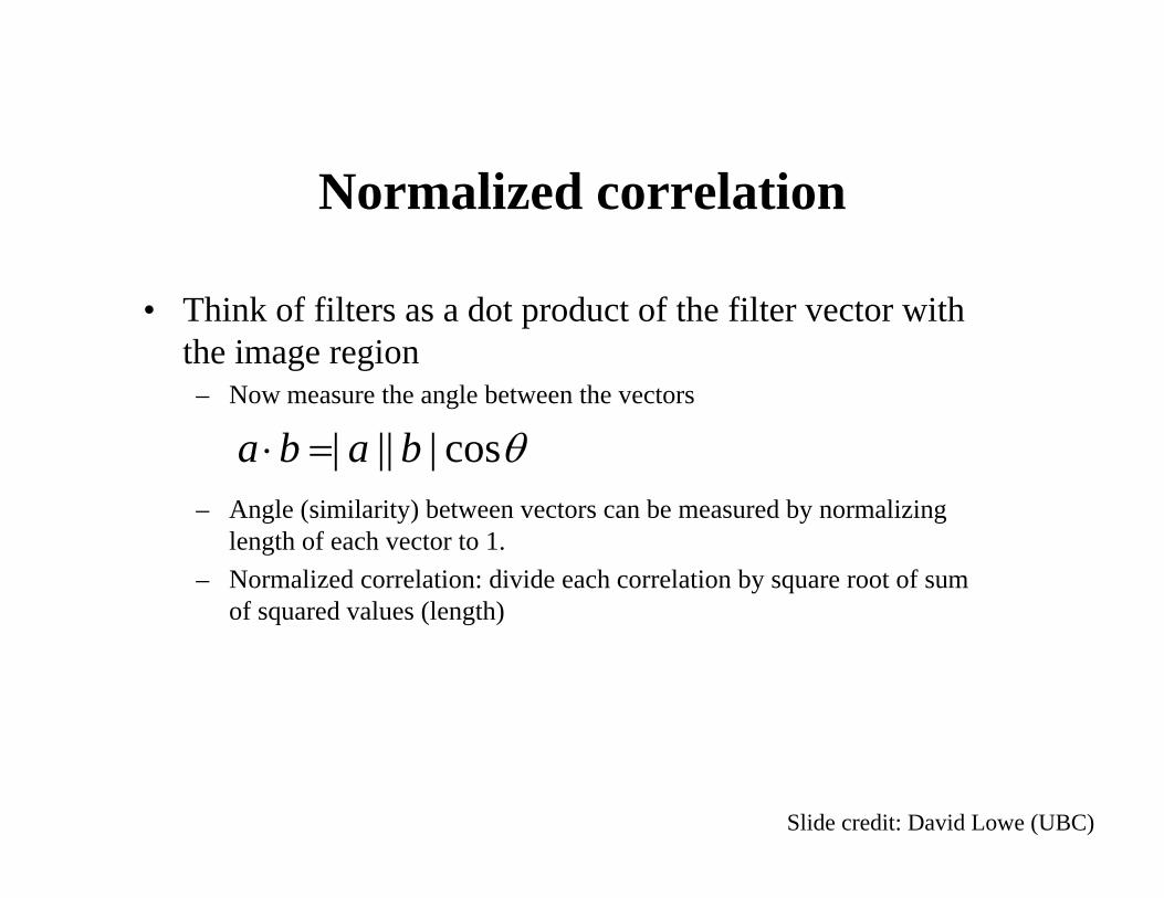
Normalized correlation
• Think of filters as a dot product of the filter vector with the image region
– Now measure the angle between the vectors
– Angle (similarity) between vectors can be measured by normalizing length of each vector to 1.
– Normalized correlation: divide each correlation by square root of sum of squared values (length)
θcos|||| baba =⋅
Slide credit: David Lowe (UBC)

Figure from “Computer Vision for Interactive Computer Graphics,” W.Freeman et al, IEEE Computer Graphics and Applications, 1998 copyright 1998, IEEE
Application: Vision system for TV remote control
- uses template matching

We need scaled representations
• Find template matches at all scales– e.g., when finding hands or faces, we don’t know what
size they will be in a particular image– Template size is constant, but image size changes
• Efficient search for correspondence– look at coarse scales, then refine with finer scales– much less cost, but may miss best match
• Examining all levels of detail– Find edges with different amounts of blur– Find textures with different spatial frequencies (levels
of detail)
Slide credit: David Lowe (UBC)
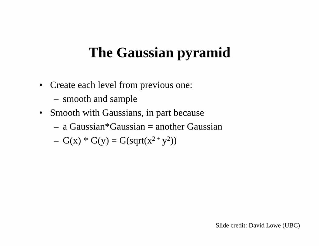
The Gaussian pyramid
• Create each level from previous one:– smooth and sample
• Smooth with Gaussians, in part because– a Gaussian*Gaussian = another Gaussian – G(x) * G(y) = G(sqrt(x2 + y2))
Slide credit: David Lowe (UBC)

All the extra levels add very little overhead for memory or computation!
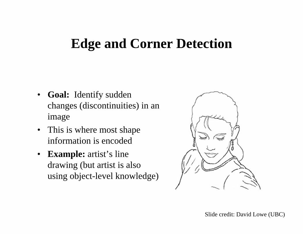
Edge and Corner Detection
• Goal: Identify sudden changes (discontinuities) in an image
• This is where most shape information is encoded
• Example: artist’s line drawing (but artist is also using object-level knowledge)
Slide credit: David Lowe (UBC)
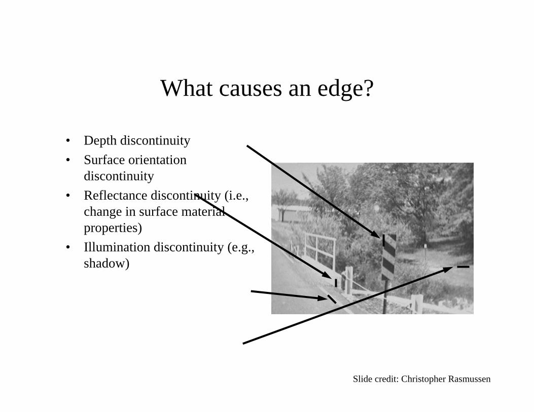
What causes an edge?
• Depth discontinuity• Surface orientation
discontinuity• Reflectance discontinuity (i.e.,
change in surface material properties)
• Illumination discontinuity (e.g., shadow)
Slide credit: Christopher Rasmussen

Smoothing and Differentiation
• Edge: a location with high gradient (derivative)• Need smoothing to reduce noise prior to taking derivative• Need two derivatives, in x and y direction. • We can use derivative of Gaussian filters
• because differentiation is convolution, and convolution is associative:
D * (G * I) = (D * G) * I

Derivative of Gaussian
Slide credit: Christopher Rasmussen
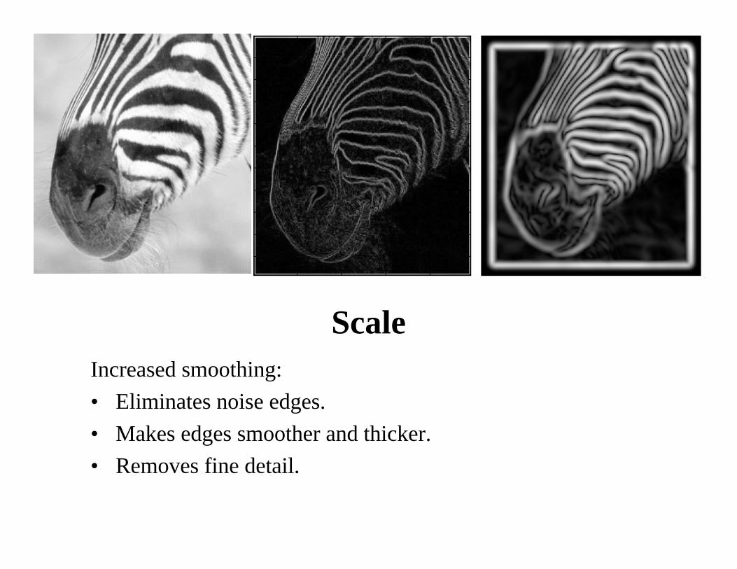
ScaleIncreased smoothing:• Eliminates noise edges.• Makes edges smoother and thicker.• Removes fine detail.
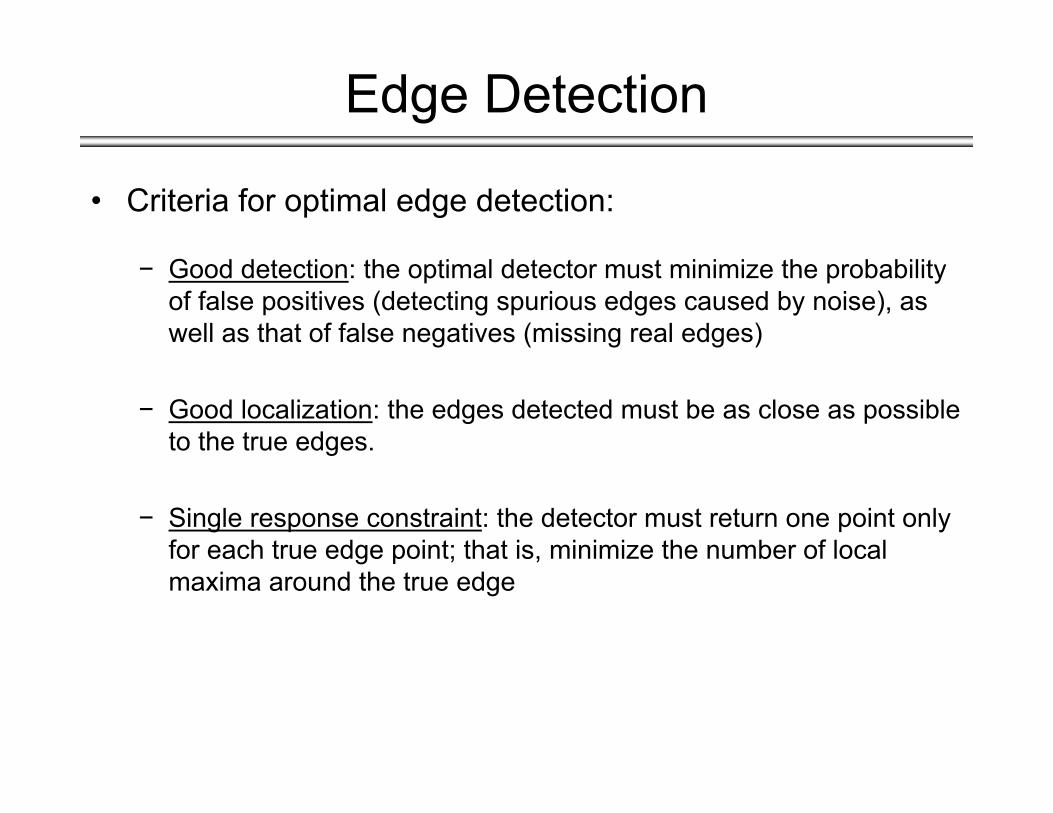
Edge Detection
− Good detection: the optimal detector must minimize the probability of false positives (detecting spurious edges caused by noise), as well as that of false negatives (missing real edges)
− Good localization: the edges detected must be as close as possible to the true edges.
− Single response constraint: the detector must return one point only for each true edge point; that is, minimize the number of local maxima around the true edge
• Criteria for optimal edge detection:
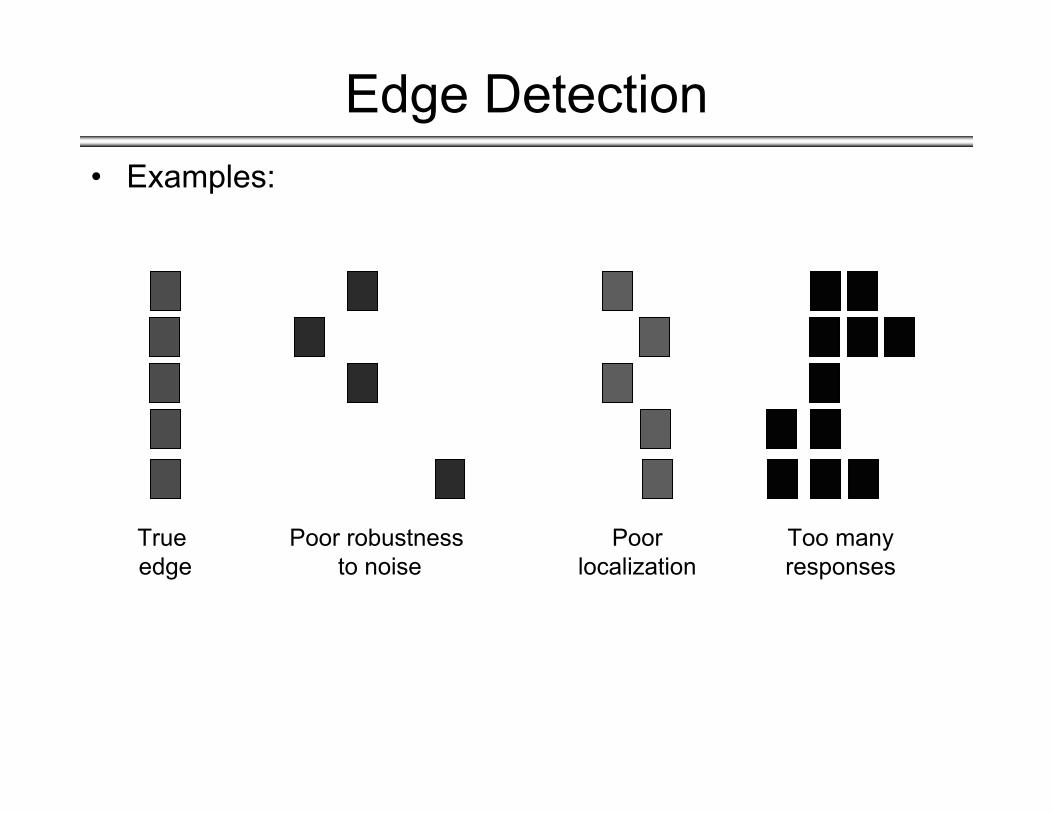
Edge Detection• Examples:
True edge
Poor robustness to noise
Poorlocalization
Too manyresponses
− This is probably the most widely used edge detector in computer vision.
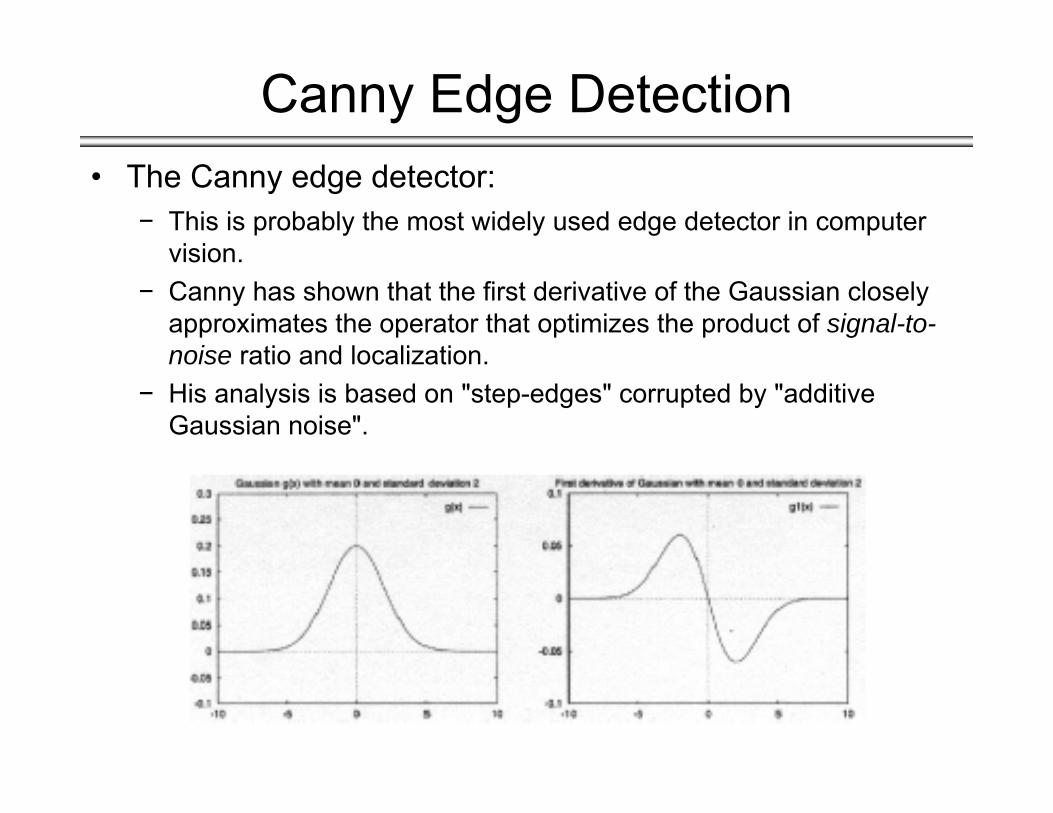
− Canny has shown that the first derivative of the Gaussian closely approximates the operator that optimizes the product of signal-to-noise ratio and localization.
− His analysis is based on "step-edges" corrupted by "additive Gaussian noise".
• The Canny edge detector:
Canny Edge Detection
Canny Edge Detection
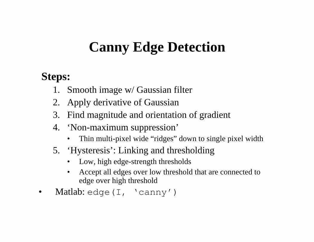
Steps:1. Smooth image w/ Gaussian filter2. Apply derivative of Gaussian3. Find magnitude and orientation of gradient4. ‘Non-maximum suppression’
• Thin multi-pixel wide “ridges” down to single pixel width5. ‘Hysteresis’: Linking and thresholding
• Low, high edge-strength thresholds• Accept all edges over low threshold that are connected to
edge over high threshold• Matlab: edge(I, ‘canny’)
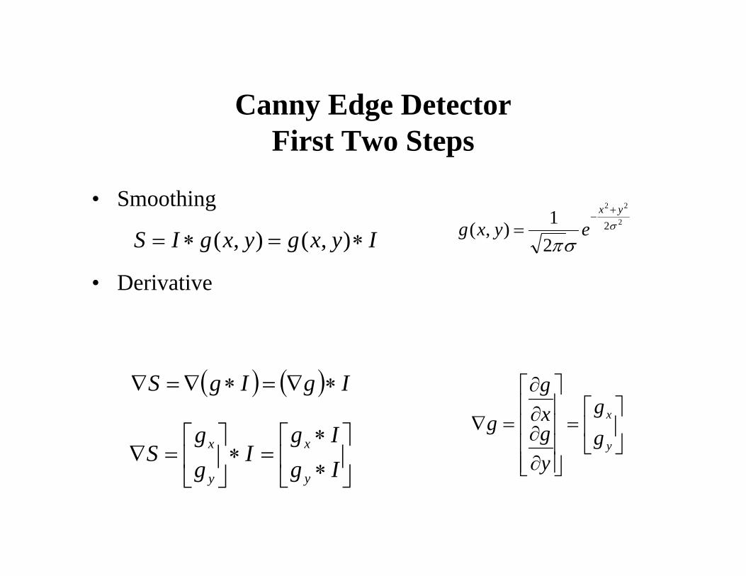
Canny Edge DetectorFirst Two Steps
• Smoothing
• Derivative
IyxgyxgIS ∗=∗= ),(),(2
22
2
21),( σ
σπ
yx
eyxg+
−=
( ) ( ) IgIgS ∗∇=∗∇=∇
⎥⎦
⎤⎢⎣
⎡=
⎥⎥⎥⎥
⎦
⎤
⎢⎢⎢⎢
⎣
⎡
∂∂∂∂
=∇y
x
gg
ygxg
gI
gg
Sy
x ∗⎥⎦
⎤⎢⎣
⎡=∇ ⎥
⎦
⎤⎢⎣
⎡∗∗
=IgIg
y
x
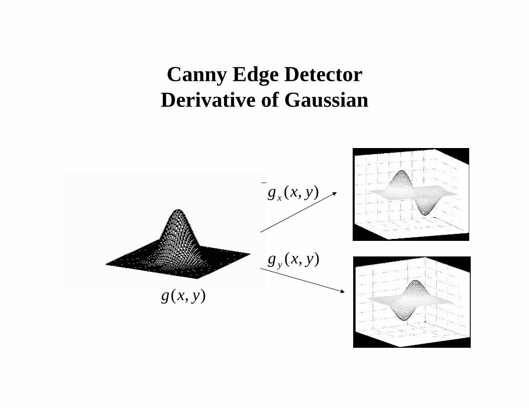
Canny Edge DetectorDerivative of Gaussian
),( yxg
),( yxgx
),( yxg y
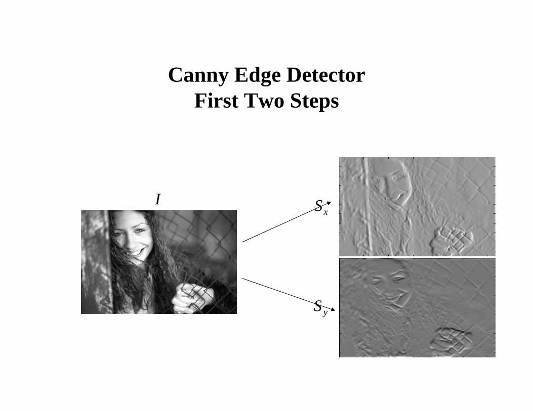
Canny Edge DetectorFirst Two Steps
xS
yS
I

Canny Edge DetectorThird Step
• Gradient magnitude and gradient direction
x
y
yx
yx
SS
SS
SS
1
22
tan
)(
),(
−==
+=
θdirection
magnitude
VectorGradient
image gradient magnitude

Canny Edge DetectorFourth Step
• Non maximum suppression
We wish to mark points along the curve where the magnitude is biggest. We can do this by looking for a maximum along a slice normal to the curve (non-maximum suppression). These points should form a curve. There are then two algorithmic issues: at which point is the maximum, and where is the next one?
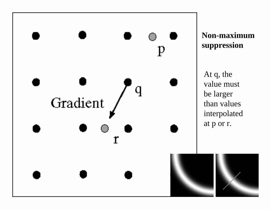
Non-maximumsuppression
At q, the value must be larger than values interpolated at p or r.

Examples: Non-Maximum Suppression
courtesy of G. Loy
Original image Gradient magnitude Non-maxima suppressed
Slide credit: Christopher Rasmussen
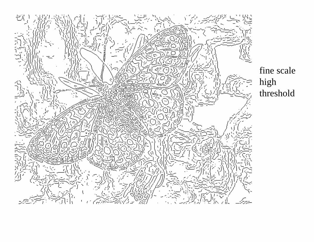
fine scalehigh threshold
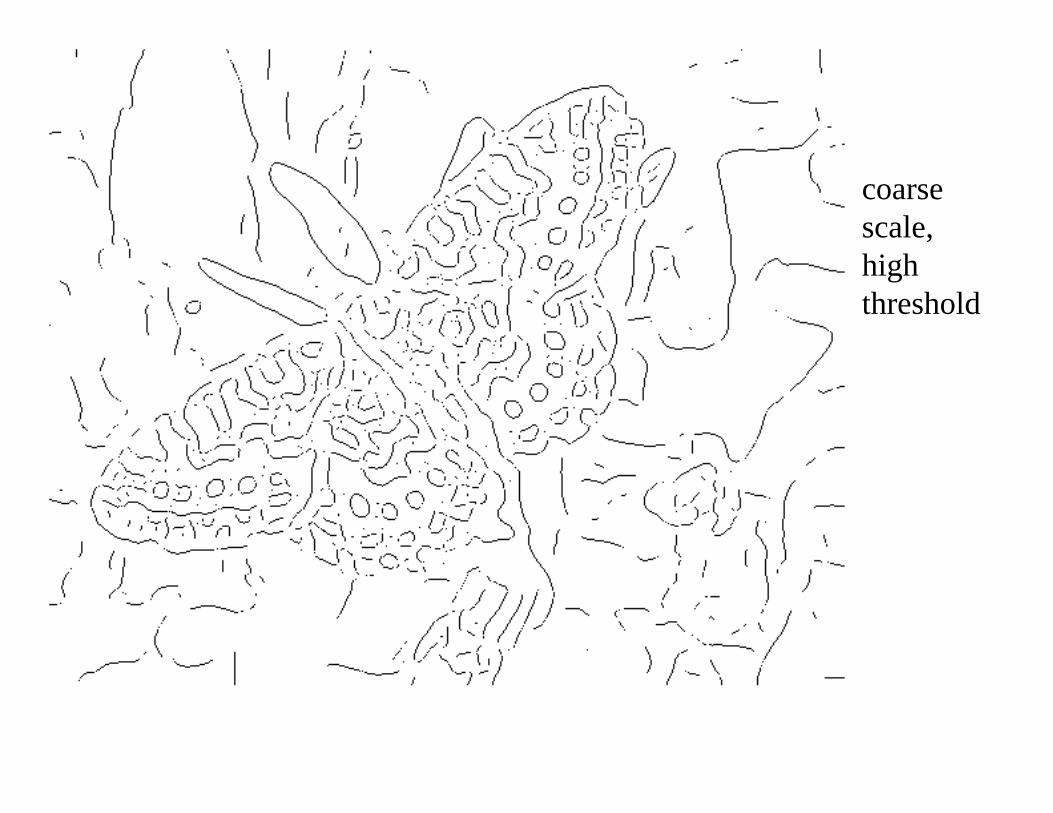
coarse scale,high threshold
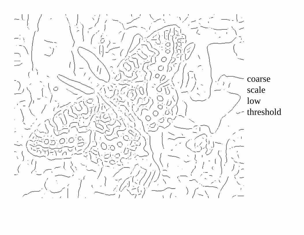
coarsescalelowthreshold
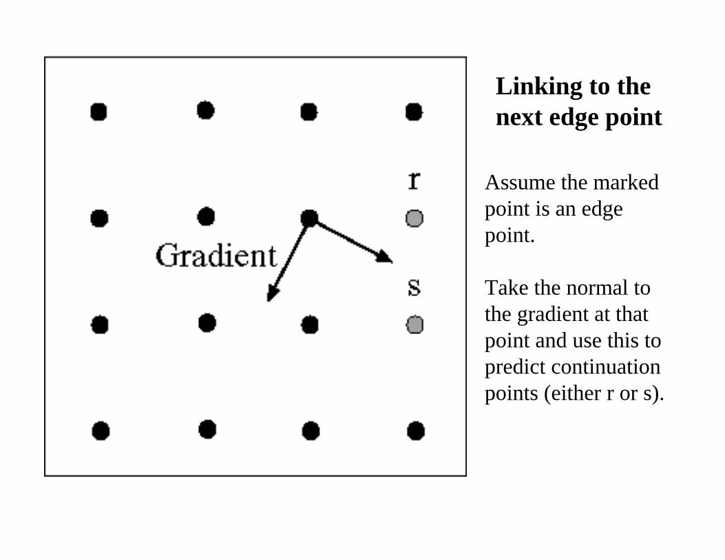
Linking to the next edge point
Assume the marked point is an edge point.
Take the normal to the gradient at that point and use this to predict continuation points (either r or s).
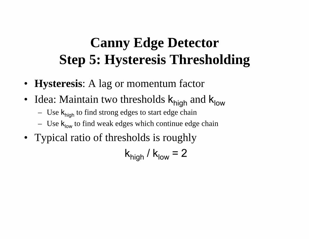
• Hysteresis: A lag or momentum factor• Idea: Maintain two thresholds khigh and klow
– Use khigh to find strong edges to start edge chain– Use klow to find weak edges which continue edge chain
• Typical ratio of thresholds is roughlykhigh / klow = 2
Canny Edge DetectorStep 5: Hysteresis Thresholding
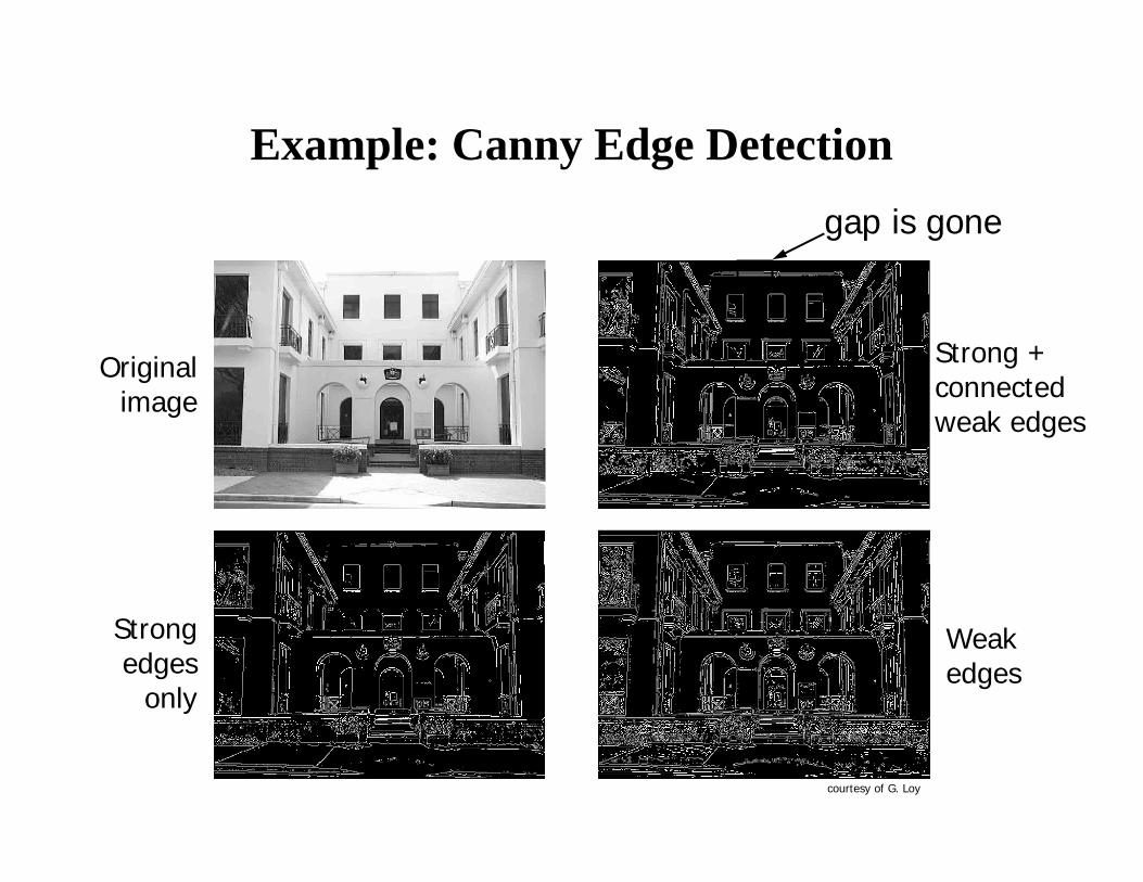
Example: Canny Edge Detection
courtesy of G. Loy
gap is gone
Originalimage
Strongedges
only
Strong +connectedweak edges
Weakedges