lecture no. 7 finite element methodcoast.nd.edu/jjwteach/www/www/60130/new lecture... · lecture...

C E 6 0 1 3 0 F I N I T E E L E M E N T M E T H O D S - L E C T U R E 7 P a g e 1 | 32

Lecture no. 7

Finite Element Method

Define the approximating functions locally over “finite elements”

Advantages

It’s much easier to satisfy the b.c.’s with local functions over local parts of the boundary

than it is with global functions over the entire boundary.

Splitting the domain into intervals and using lower order approximations within each

element will cause the integral error to assure better accuracy on a pointwise basis.

(Courant, 1920).

An integral norm attempts to minimize total error over the entire domain. A low integral

norm does not always mean that we have good pointwise error norm.


General Steps to FEM

Divide the domain into N sub-intervals or finite elements.

Develop interpolating functions valid over each element. We will make use of localized

coordinate systems to assure functional universality (i.e. they will be applicable to any

length element at any location).

We will tailor these functions such that the required degree of functional continuity can

be readily enforced.

Enforce functional continuity

Through definition of Cardinal basis

Through “global” matrix assembly

Note that we use these interpolating functions in conjunction with the implementation of

the desired weighted residual form (i.e. integrations etc.) as before.


Lagrange Interpolation

Lagrange Interpolation : pass an approximating function, g(x), exactly through the

functional values at a set of interpolation points or nodes.


Method 1 to deriving g(x) – Power series:

─ We are given 𝑓0, 𝑓1, 𝑓2 and corresponding points 𝑥0, 𝑥1, 𝑥2

─ Constraints we can apply

𝑔(𝑥0 = 0) = 𝑓0

𝑔(𝑥1 = ℎ) = 𝑓1

𝑔(𝑥2 = 2ℎ) = 𝑓2

3 Constraints ⇒ 3 d.o.f/3 nodes = 1 d.o.f/node

⇒ Polynomial form g(x) can have 3 d.o.f ⇒ quadratic

─ General form of g(x)

𝑔(𝑥) = 𝑎 + 𝑏𝑥 + 𝑐𝑥2

─ Apply constraints

𝑔(𝑥0 = 0) = 𝑓0 ⇒ 𝑎 = 𝑓0

𝑔(𝑥1 = ℎ) = 𝑓1 ⇒ 𝑎 + 𝑏ℎ + 𝑐ℎ2 = 𝑓1

𝑔(𝑥2 = 2ℎ) = 𝑓2 ⇒ 𝑎 + 2ℎ𝑏 + 4ℎ2𝑐 = 𝑓2


Solve a system of simultaneous equations.

[1 0 01 1 11 2 4

] [𝑎𝑏ℎ𝑐ℎ2]=[

𝑓0𝑓1𝑓2

] ⇒

[𝑎𝑏ℎ𝑐ℎ2] = [

1 0 0−1.5 2 −0.50.5 −1 0.5

] [

𝑓0𝑓1𝑓2

] ⇒

𝑎 = 𝑓0

𝑏 =1

ℎ(−

3

2 𝑓0 + 2𝑓1 −

1

2𝑓2)

𝑐 =1

ℎ2(1

2𝑓0 − 𝑓1 +

1

2𝑓2)

∴ 𝑔(𝑥) = 𝑓0 +1

2ℎ(−3𝑓0 + 4𝑓1 − 𝑓2)𝑥 +

1

2ℎ2(𝑓0 − 2𝑓1 + 𝑓2)𝑥

2

Interpolating function throughout interval of interest [0,2ℎ]


Let’s rewrite 𝑔(𝑥)

Factor out of 𝑓0, 𝑓1 and 𝑓2

𝑔(𝑥) = 𝑓0 (1 −3𝑥

2ℎ𝑥 +

1

2ℎ2𝑥2)⏟

≡𝜙0(𝑥)

+ 𝑓1 (4

2ℎ𝑥 −

1

ℎ2𝑥2)⏟

≡𝜙1(𝑥)

+ 𝑓2 (−1

2ℎ𝑥 +

1

2ℎ2𝑥2)⏟

≡𝜙2(𝑥)

⇒

𝑔(𝑥) = ∑ 𝑓𝑖 𝜙𝑖(𝑥)⏟ →

2𝑖=0

Interpolating basis functions!!

Each is associated with one node.

Looks very much like expansions we used for w.r. methods!!!

Let’s plot these functions

𝜙0(𝑥0 = 0) = 1 𝜙1(𝑥0 = ∅) = 0 𝜙2(𝑥0 = 0)

𝜙0(𝑥1 = ℎ) = 0 𝜙1(𝑥1 = ℎ) = 1 𝜙2(𝑥1 = ℎ) = 0

𝜙0(𝑥1 = 2ℎ) = 0 𝜙1(𝑥2 = 2ℎ) = 0 𝜙2(𝑥2 = 2ℎ) = 1


Thus 𝜙1(𝑥𝑗) = 𝛿𝑖𝑗 =1 𝑖 = 𝑗0 𝑖 ≠ 𝑗

⇒ We can in fact use the constraints to derive 𝜙0, 𝜙1

and 𝜙2

Thus interpolating functions are 1 at nodes they are associated with and zero at all other

nodes. At x values other than nodal values these functions vary and do not equal zero.

A very important consequence of using Lagrange interpolation is that

𝑔(𝑥𝑖) = 𝑓𝑖

This property and the fact that we define nodes on inter-element boundaries will enable us

to easily enforce functional continuity on inter-element boundaries


Applying Lagrange Interpolation to develop 𝒖𝒂𝒑𝒑

Option 1 – Develop a higher order approximation which is global and based on Lagrange basis

function defined over the entire domain.

𝑢𝑎𝑝𝑝 =∑𝑢𝑖𝜙𝑖

𝑁

𝑖=1

where

𝜙𝑖 = globally defined Lagrange basis functions valid over the entire domain

𝑢𝑖 = the expansion coefficients and by definition these equal the function values at the nodes!!

𝑖 = 1, 𝑁 are the N “nodes” defined throughout the global domain

These nodes can be equispaced or nonequispaced


Boundary conditions can be readily incorporated into the expansion if they are function

specified (essential type boundary conditions)

─ For example 𝑢(𝑥𝐿) = 𝑢𝐿

𝑢(𝑥𝑅) = 𝑢𝑅

─ The expansion can now be written as

𝑢𝑎𝑝𝑝 = 𝑢𝐿𝜙1 + 𝑢𝑅𝜙𝑁 + ∑ 𝑢𝑖𝜙𝑖

𝑁−1

𝑖=2

(since 𝑢1 = 𝑢𝐿 and 𝑢𝑁 = 𝑢𝑅)

─ Thus

𝑢𝐵 = 𝑢𝐿𝜙1 + 𝑢𝑅𝜙𝑁

─ We note that 𝑢𝐵 satisfies admissibility conditions

𝑢𝐵(𝑥𝐿) = 𝑢𝐿 𝜙1(𝑥𝐿)⏟ =1

+ 𝑢𝑅 𝜙𝑁(𝑥𝐿)⏟ =0

= 𝑢𝐿

𝑢𝐵(𝑢𝑅) = 𝑢𝐿 𝜙1(𝑥𝑅)⏟ =0

+ 𝑢𝑅 𝜙𝑁(𝑥𝑅)⏟ =1

= 𝑢𝑅


─ Also we note that the remaining 𝜙𝑖 𝑖 = 2, 𝑁 − 1 satisfy

𝜙𝑖(𝑥𝐿) = 0 →

𝜙𝑖(𝑥𝑅) = 0 𝑖 = 2, 𝑁 − 1

Thus satisfying function specified b.c.’s (essential) for 1-D is very easy!! For natural b.c.’s

it is much more difficult.

The sequence of functions 𝜙𝑖 are linearly independent

The coefficients in the expansion are now actually equal to the values of the function at the

nodes!!

The drawback of option 1 is that you obtain poor pointwise convergence as N becomes

large for most problems.

Another drawback is that the matrix will also be almost fully populated

Typically the technique does work well for slowly varying smooth solutions.


Example

Solve 𝐿(𝑢) = 𝑝(𝑥) 𝑥 ∈ [𝑥𝐿, 𝑥𝑅]

b.c.’s 𝑢(𝑥𝐿) = 𝑢𝐿


Assume that we will apply a six term expansion

𝑢𝑎𝑝𝑝 = 𝑢𝐿𝜙1 + 𝑢𝑅𝜙6 +∑𝑢𝑖𝜙𝑖

5

𝑖=2


Note that 𝑢𝐵 = 𝑢𝐿𝜙1 + 𝑢𝑅𝜙6

𝑢𝐵 satisfies b.c.’s as specified

Note that 𝜙2, 𝜙3, 𝜙4 and 𝜙5 all satisfy the homogeneous form of the essential

function specified b.c.’s


Option 2 – Develop an approximation 𝑢𝑎𝑝𝑝 which is the sum of localized approximations

𝑢𝑎𝑝𝑝 = ∑∑𝑢𝑖𝑗𝜙𝑖𝑗

𝑁𝑗

𝑖=1

𝑀

𝑗=1

Where 𝑢𝑖𝑗= expansion coefficient for element j and node i within element j

𝜙𝑖𝑗= Lagrange basis function for element j and node i

Note that 𝜙𝑖𝑗= 0 outside of element j

𝑗 = 1,𝑀 = total number of localized domains or “finite elements”

𝑖 = 1, 𝑁𝑗 = total number of nodes within element j


Local unknowns at nodes

𝑢11 𝑢3

1 𝑢31 𝑢1

3 𝑢23 𝑢3

3 𝑢43 𝑢5

3 𝑢63

𝑢12 𝑢2

2 𝑢32 𝑢1

4 𝑢24 𝑢3

4 ← 𝑒𝑙𝑒𝑚𝑒𝑛𝑡 𝑖𝑛𝑑𝑒𝑥 ← 𝑙𝑜𝑐𝑎𝑙 𝑛𝑜𝑑𝑒 𝑖𝑛𝑑𝑒𝑥

The boundary conditions can again be readily built into 1-D type problems for function

specified conditions (essential). Even in multiple dimensions, function specified b.c.’s

(essential) can be incorporated in a straight forward manner

The sequence of all functions will be linearly independent.

Again note that those coeficients of expansion are equal to the actual function values at the

nodes


To ensure 𝐶0 inter-element functional continuity we must have at all inter-element

boundaries:

𝑢𝑎𝑝𝑝(left of an inter-element boundary) = 𝑢𝑎𝑝𝑝 (right of an inter-element boundary)

Thus in the example given

Anywhere in element 1

𝑢1(𝜉) = 𝑢11𝜙11(𝜉) + 𝑢2

1𝜙21(𝜉) + 𝑢3

1𝜙31(𝜉)

Note that all other Lagrange basis function from other elements are defined as zero.

Anywhere in element 2

𝑢2(𝜉) = 𝑢12𝜙12(𝜉) + 𝑢2

2𝜙22(𝜉) + 𝑢3

1𝜙32(𝜉)

Element 1 evaluated at r.h.s.

𝑢1(𝜉31) = 𝑢3

1

Element 2 evaluated at l.h.s.

𝑢2(𝜉12) = 𝑢1

2

In order to enforce 𝑐0 functional continuity we must have

𝑢1(𝜉31) = 𝑢2(𝜉1

2)


∴ 𝑢31 = 𝑢1

2

In general we must have the expansion coefficients equal at inter-element boundaries in

order to satisfy 𝑐0 functional continuity requirements

In our example, the expansion coef.’s are related as

𝑢31 = 𝑢1

2

𝑢32 = 𝑢1

3

𝑢63 = 𝑢1

4

∴ We must have expansion coef.’s at inter-element boundaries be equal

There are several approaches to implement the inter-element functional continuity (i.e.

setting equal the adjacent inter-element expansion coef.’s)

─ Develop “Cardinal” basis functions which are formed by patching together the

localized Lagrange functions and defining them globally. This also implies that you

redefine the expansion coef.’s globally (so that there will now be only one coef. per

global node)

─ Actually implement all expansions locally. Then take care of inter-element functional

continuity by assembling the “global” matrix correctly


Notes

Boundary condition implementation/satisfaction as well as inter-element functional

continuity enforcement are made simple and possible by the use of Lagrange basis

functions. However we must place nodes at the ends of the domain as well as at the ends of

each element for this to work.

The advantages of defining local functions are:

─ Essential function specified b.c.’s are very easy to implement in 2-D and 3-D as well

as 1-D

─ Excellent pointwise as well as integral norm convergence

─ Matrices are sparse with a limited number of non-zero entries per row


Solve 𝐿(𝑢) = 𝑝(𝑥) [𝑥𝐿, 𝑥𝑅]

𝑢(𝑥𝐿) = 𝑢𝐿


Consider the following 6 global nodes defined over 4 elements


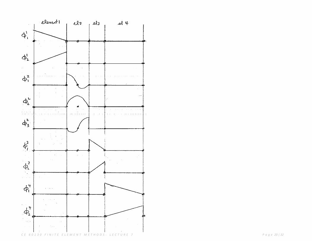
We will have the following elemental based expansion

part of uB ↓ ↓ elemental index

𝑢𝑎𝑝𝑝 = 𝑢𝐿𝜙11 + 𝑢2

1𝜙21 Element 1

↑ ↑ local node index

+ 𝑢12𝜙12 + 𝑢2

2𝜙22 + 𝑢3

2𝜙32 Element 2

+ 𝑢13𝜙13 + 𝑢2

3𝜙23 Element 3

+ 𝑢14𝜙14 + 𝑢𝑅𝜙2

4 ← part of 𝑢𝐵 Element 4

This is a local expansion!!

It has 7 elemental unknowns

However 3 functional continuity constraints will be applied


We can also patch together functions and form truly “global” functions. These are called

“Cardinal” bases

part of 𝑢𝐵

𝑢𝑎𝑝𝑝 = 𝑢𝐿𝛷𝑛1⏞ + 𝑢𝑛2𝛷𝑛2 + 𝑢𝑛3𝛷𝑛3 + 𝑢𝑛4𝛷𝑛4

+𝑢𝑛5𝛷𝑛5 + 𝑢𝑅𝛷𝑛6 ← part of 𝑢𝐵

𝛷𝑛1 = 𝜙11 𝑢𝑛1 = 𝑢1

1 = 𝑢𝐿 essential b.c

𝛷𝑛2 = 𝜙21 + 𝜙1

2 𝑢𝑛2 = 𝑢21 = 𝑢1

2 unknown

𝛷𝑛3 = 𝜙22 𝑢𝑛3 = 𝑢2

2 unknown

𝛷𝑛4 = 𝜙32 + 𝜙1

3 𝑢𝑛4 = 𝑢32 = 𝑢1

3 unknown

𝛷𝑛5 = 𝜙23 + 𝜙1

4 𝑢𝑛5 = 𝑢23 = 𝑢1

4 unknown

𝛷𝑛6 = 𝜙24 ⏟ 𝑢𝑛6 = 𝑢2

4 = 𝑢𝑅⏟ essential b.c.

local functions local coef.’s or unknown functions

↑ Cardinal or global functions ↑ Global coef.’s or unknown functions


Notes

• The global or Cardinal basis functions and approximation automatically satisfy

functional continuity. This is not true for local expansions for which we must still enforce

the functional continuity constraints.

• However it will be very easy to handle the functional continuity constraints and it is much

easier to work with the local functions in a finite element grid.


• Global basis functions


Local Lagrange basis functions

Define a “unit” element with a local coordinate system

−1 ≤ 𝜉 ≤ +1

Map the element j which lies in the interval 𝑥𝑗 ≤ 𝑥 ≤ 𝑥𝑗+1 to the unit element.

The transformation and its inverse are:

𝜉 = −1 + 2(𝑥 − 𝑥𝑗)/(𝑥𝑗+1 − 𝑥𝑗)

and

𝑥 = 𝑥𝑗 + (𝑥𝑗+1 − 𝑥𝑗)(𝜉 + 1)/2

Define the function associated with each node in a local coordinate system:

𝜙1(𝜉) = 𝑎1 + 𝑏1𝜉

𝜙2(𝜉) = 𝑎2 + 𝑏2𝜉


Apply constraints to solve for the coefficients

𝜙1(𝜉1) = 1 𝜙1(𝜉2) = 0

𝜙2(𝜉1) = 0 𝜙2(𝜉2) = 1

This leads to:

𝜙1(𝜉) =1

2(1 − 𝜉)

𝜙2(𝜉) =1

2(1 + 𝜉)

These functions represent the linear Lagrange interpolation functions. These allow

𝑪𝒐 functional continuity and each local basis function equals unity at the associated

node and zero elsewhere.


These local basis functions on the unit element are related to those defined over the 𝑗𝑡ℎ

element by

𝜙1(𝜉) = 𝜙2𝑗−1(𝑥(𝜉)) = 𝜙2𝑗−1(𝑥)

𝜙2(𝜉) = 𝜙2𝑗(𝑥(𝜉)) = 𝜙2𝑗(𝑥)

where 𝜙2𝑗−1(𝑥) and 𝜙2𝑗(𝑥) are defined as nonzero for 𝑥𝑗 ≤ 𝑥 ≤ 𝑥𝑗+1 and zero everywhere

else.

We note that

�̂�𝑒 = α1𝜙1(𝜉) + α2𝜙2(𝜉)

Therefore:

�̂�𝑒(𝜉1) = α1 �̂�𝑒(𝜉2) = α2

Therefore the coefficients of the elemental expansion equals the actual value of the

function at the nodes!


Derivatives of 𝜙2𝑗−1(𝑥) w.r.t. x

𝑑𝜙2𝑗−1

𝑑𝑥=𝑑𝜙1𝑑𝑥

=𝑑𝜙1𝑑𝜉

𝑑𝜉

𝑑𝑥=

2

(𝑥𝑗+1 − 𝑥𝑗)

𝑑𝜙1𝑑𝜉

and

𝑑𝜙2𝑗

𝑑𝑥=

2

(𝑥𝑗+1 − 𝑥𝑗)

𝑑𝜙2𝑑𝜉

Note that these formula are valid whether or not elements of equal length are used. If

(𝑥𝑗+1 − 𝑥𝑗) = ∆𝑥 is constant, then derivatives of the basis functions w.r.t., 𝑑𝜙𝑗/𝑑𝑥, are

related by the constant 2/∆𝑥 to the derivatives w.r.t. 𝜉 of these functions.

Cardinal Basis Functions:

If we piece together the elemental functions such that we eliminate or satisfy the

functional continuity requirements we form the cardinal basis functions:

𝛷𝑖(𝑥) = chapeau functions (also called rooftop or tophat functions)


Previously we had:

𝑢𝑎𝑝𝑝 = ∑ 𝑢1𝑒𝑙𝑗𝑁

𝑒𝑙𝑗=1𝜙1𝑒𝑙𝑗 + 𝑢2

𝑒𝑙𝑗𝜙2𝑒𝑙𝑗

with 2N unknowns when N=the no. of elements

Now we’ve enforced functional continuity by

i. requiring 𝑢2𝑒𝑙1 = 𝑢1

𝑒𝑙2 = 𝑢2global

etc.

ii. defining 𝛷2 = 𝜙2𝑒𝑙1 + 𝜙1

𝑒𝑙2 etc.

Thus we have N-1 constraints and we can now write

𝑢𝑎𝑝𝑝(𝑥) = ∑ (𝑢𝑖global

𝛷𝑖)

𝑁+1

𝑖=1

We now have N+1 unknowns which equals the total number of nodes.

Therefore the rooftop functions are the same as the first order polynomials defined over

each element except that now the functional continuity requirement is automatically

satisfied.

In FE practice we don’t really use Cardinal basis functions. We use the local elemental

functions and account for functional continuity as matrix assembly proceeds.


Development of Lagrange Quadratic Basis

𝐶𝑜 functional continuity using quadratic interpolation over an element (instead of the

required minimum linear), requires 3 nodes per element.

Consider the unit element and let the 3 nodes be defined such that 𝜉1 = −1,

𝜉2 = 0, and 𝜉3 = +1.

The general form of the Lagrange quadratic basis function is:

𝜙𝑖(𝜉) = 𝑎𝑖 + 𝑏𝑖𝜉 + 𝑐𝑖𝜉2, 𝑖 = 1,3

and the elemental expansion is

�̂�𝑒 =∑𝑢𝑖𝜙𝑖

3

𝑖=1

We now require that 𝜙𝑖(𝜉𝑗) = 𝛿𝑖𝑗 , 𝑖 = 1,3; 𝑗 = 1,3 (this defines 9 constraints to solve

for the 9 unknowns).


Thus:

𝜙11(−1) = 𝑎1 − 𝑏1 + 𝑐1 = 1

𝜙11(0) = 𝑎1 = 0

𝜙11(+1) = 𝑎1 + 𝑏1 + 𝑐1 = 0

Hence:

𝑎1 = 0, 𝑏1 = −1

2, 𝑐1 =

1

2

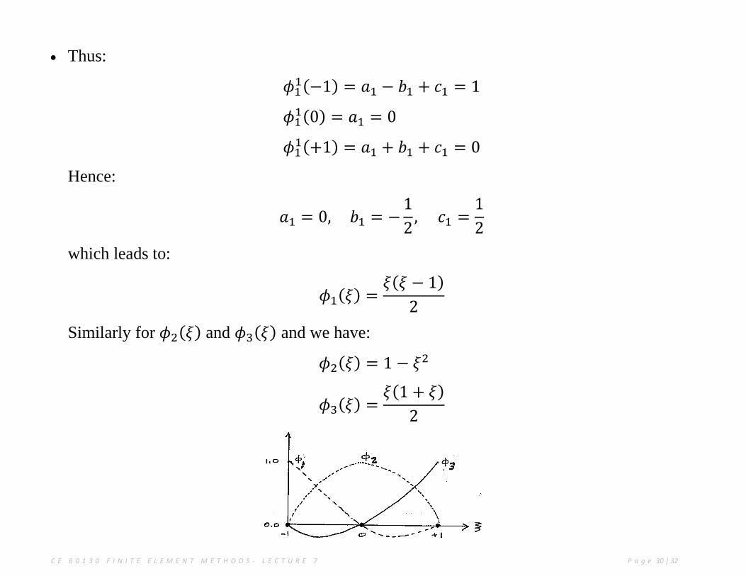
which leads to:

𝜙1(𝜉) =𝜉(𝜉 − 1)

2

Similarly for 𝜙2(𝜉) and 𝜙3(𝜉) and we have:

𝜙2(𝜉) = 1 − 𝜉2

𝜙3(𝜉) =𝜉(1 + 𝜉)

2


Notes

Again we note that the generic expansion is written over each element as

�̂�𝑒𝑙 = 𝑢1𝑒𝑙𝜙1(𝜉) + 𝑢2

𝑒𝑙𝜙2(𝜉) + 𝑢3𝑒𝑙𝜙3(𝜉)

Thus the coefficients in the expansion for �̂�𝑒 equal the value of the function at the node 𝜉𝑖.

This is only possible sue to the form of the basis/expansion functions!

We still only have 𝐶𝑜 functional continuity between elements. We do have non-trivial 2nd

derivatives within the element. However the 2nd derivatives are not defined at inter-element

boundaries!

Cardinal Basis

# of elemental unknowns 3𝑁

# of functional continuity constraints 𝑁 − 1

Total number of global unknowns 2𝑁 + 1

We have

N+1 vertex nodes

N mid-side nodes

2N+1 total number of globally defined basis functions

Note that 2N + 1 also equals the total number of nodes for N elements.


Piecing together the element functions we arrive at the following set of 2N + 1

Cardinal basis functions:

Each function is associated with 1 global node and is defined such that inter-element

continuity is assured.

𝑢𝑎𝑝𝑝(𝑥) = ∑ 𝑢𝑖𝛷𝑖(𝑥)

2𝑁+1

𝑖=1

Higher Order Lagrange Interpolation can be treated in similar ways

1. Add more nodes which allows us to define more interpolating functions of higher order.

2. Require each interpolating function to be equal to unity at the node it is associated with

and zero at all other nodes

3. The unknown coefficients will equal the functional value at the nodes!

lecture no. 7 finite element methodcoast.nd.edu/jjwteach/www/www/60130/new lecture... · lecture...

Documents