lecture notes mathematical foundations for finance
TRANSCRIPT

Lecture Notes
Mathematical Foundations
for Finance
© M. Schweizer and E. W. Farkas
Department of Mathematics
ETH Zurich
This version: December 15, 2020


Contents
1 Financial markets in finite discrete time 5
1.1 Basic probabilistic concepts . . . . . . . . . . . . . . . . . . . . . . . . . . 5
1.2 Financial markets and trading . . . . . . . . . . . . . . . . . . . . . . . . . 9
1.3 Some important martingale results . . . . . . . . . . . . . . . . . . . . . . 21
1.4 An example: The multinomial model . . . . . . . . . . . . . . . . . . . . . 26
2 Arbitrage and martingale measures 31
2.1 Arbitrage . . . . . . . . . . . . . . . . . . . . . . . . . . . . . . . . . . . . 31
2.2 The fundamental theorem of asset pricing . . . . . . . . . . . . . . . . . . 39
2.3 Equivalent (martingale) measures . . . . . . . . . . . . . . . . . . . . . . . 45
3 Valuation and hedging in complete markets 51
3.1 Attainable payo↵s . . . . . . . . . . . . . . . . . . . . . . . . . . . . . . . . 51
3.2 Complete markets . . . . . . . . . . . . . . . . . . . . . . . . . . . . . . . . 59
3.3 Example: The binomial model . . . . . . . . . . . . . . . . . . . . . . . . . 62
4 Basics about Brownian motion 69
4.1 Definition and first properties . . . . . . . . . . . . . . . . . . . . . . . . . 69
4.2 Martingale properties and results . . . . . . . . . . . . . . . . . . . . . . . 76
4.3 Markovian properties . . . . . . . . . . . . . . . . . . . . . . . . . . . . . . 82
5 Stochastic integration 85
5.1 The basic construction . . . . . . . . . . . . . . . . . . . . . . . . . . . . . 86
5.2 Properties . . . . . . . . . . . . . . . . . . . . . . . . . . . . . . . . . . . . 97
5.3 Extension to semimartingales . . . . . . . . . . . . . . . . . . . . . . . . . 101
6 Stochastic calculus 105
6.1 Ito’s formula . . . . . . . . . . . . . . . . . . . . . . . . . . . . . . . . . . . 105
6.2 Girsanov’s theorem . . . . . . . . . . . . . . . . . . . . . . . . . . . . . . . 117
6.3 Ito’s representation theorem . . . . . . . . . . . . . . . . . . . . . . . . . . 124

CONTENTS 4
7 The Black–Scholes formula 127
7.1 The Black–Scholes model . . . . . . . . . . . . . . . . . . . . . . . . . . . . 127
7.2 Markovian payo↵s and PDEs . . . . . . . . . . . . . . . . . . . . . . . . . 134
7.3 The Black–Scholes formula . . . . . . . . . . . . . . . . . . . . . . . . . . . 138
8 Appendix: Some basic concepts and results 143
8.1 Very basic things . . . . . . . . . . . . . . . . . . . . . . . . . . . . . . . . 143
8.2 Conditional expectations: A survival kit . . . . . . . . . . . . . . . . . . . 146
8.3 Stochastic processes and functions . . . . . . . . . . . . . . . . . . . . . . . 150
9 References 151
10 Index 153

1 FINANCIAL MARKETS IN FINITE DISCRETE TIME 5
1 Financial markets in finite discrete time
In this chapter, we introduce basic concepts in order to model trading in a frictionless
financial market in finite discrete time. We recall the required notions from probability
theory and stochastic processes and directly illustrate them by means of examples.
Standard concepts and results from (measure-theoretic) probability theory are as-
sumed to be known; Chapter 8 contains a brief (and non-comprehensive) summary, and
details can be found in Jacod/Protter [10] or Durrett [6].
1.1 Basic probabilistic concepts
Financial markets involve uncertainty , in particular about the future evolution of asset
prices. We therefore start from a probability space (⌦,F , P ). Time evolves in discrete
steps over a finite horizon; we label trading dates as k = 0, 1, . . . , T with T 2 IN .
The flow of information over time is described by a filtration IF = (Fk)k=0,1,...,T ; this
is a family of �-fields Fk ✓ F which is increasing in the sense that Fk ✓ F` for k `.
The interpretation is that Fk contains all events that are observable up to and including
time k.
An (IRd-valued) stochastic process in this discrete-time setting is simply a family
X = (Xk)k=0,1,...,T of (IRd-valued) random variables which are all defined on the same
probability space (⌦,F , P ). This can be used to describe the random evolution over time
of d quantities, e.g. a bank account, asset prices, some liquidly traded options, or the
holdings in a portfolio of assets. A stochastic process X is called adapted (to IF ) if each
Xk is Fk-measurable, i.e. observable at time k; it is called predictable (with respect to IF )
if each Xk is even Fk�1-measurable, for k = 1, . . . , T . (For the predictable processes X
we use here, the value X0 at time 0 is usually irrelevant.)
Example. If we think of a market where assets can be traded once each day (so that
the time index k numbers days), then the price of a stock will usually be adapted because
date k prices are known at date k. But if one wants to invest by selling or buying shares,
one must make that decision before one knows where prices go in the next step; hence
trading strategies must be predictable, unless one allows insiders or prophets. For a more

1 FINANCIAL MARKETS IN FINITE DISCRETE TIME 6
detailed discussion, see Section 1.2.
Example (multiplicative model). Suppose that we start with random variables
r1, . . . , rT and Y1, . . . , YT . Take a constant S10 > 0 and define
eS0k:=
kY
j=1
(1 + rj), eS1k:= S
10
kY
j=1
Yj
for k = 0, 1, . . . , T . Note that we use here and throughout the convention that an empty
product equals 1 and an empty sum equals 0. Suppose also that rk > �1 and Yk > 0
P -a.s. for k = 1, . . . , T . Then we have
eS0k
eS0k�1
= 1 + rk,
eS1k
eS1k�1
= Yk,
or equivalently
eS0k� eS0
k�1 = eS0k�1rk,
eS1k� eS1
k�1 = eS1k�1(Yk � 1),
with eS00 = 1, eS1
0 = S10 .
Interpretation. rk describes the (simple) interest rate for the period (k � 1, k]; so eS0
models a bank account with that interest rate evolution, and rk > �1 ensures that eS0> 0,
in the sense that eS0k> 0 P -a.s. for k = 0, 1, . . . , T . Similarly, eS1 models a stock , say, and
Yk is the growth factor for the time period (k � 1, k]. Of course, we could strengthen the
analogy by writing Yk = 1+Rk; then Rk > �1 would describe the (simple) return on the
stock for the period (k � 1, k].
How about the filtration in this example? For a general discussion, see Remark 1.1
below. The most usual choice for IF is the filtration generated by Y , i.e.,
Fk = �(Y1, . . . , Yk) = �(eS10 ,eS11 , . . . ,
eS1k)
is the smallest �-field that makes all stock prices up to time k observable. Then eS1 is
obviously adapted to IF . The bank account is naturally less risky than a stock, and in

1 FINANCIAL MARKETS IN FINITE DISCRETE TIME 7
particular the interest rate for the period (k � 1, k] is usually known at the beginning,
i.e. at time k�1. So each rk ought to be Fk�1-measurable, i.e. the process r = (rk)k=1,...,T
should be predictable. Then eS0 is also predictable (and vice versa). In particular, the
interest rate rk for the period (k� 1, k] then only depends on Y1, . . . , Yk�1 or equivalently
on the stock prices eS10 ,eS11 , . . . ,
eS1k�1, but not on other factors. This can be generalised.
Example (binomial model). Suppose all the rk are constant with a value r > �1;
this means that we have the same nonrandom interest rate over each period. Then the
bank account evolves as eS0k= (1 + r)k for k = 0, 1, . . . , T .
Suppose also that Y1, . . . , YT are independent and only take two values, 1 + u with
probability p, and 1 + d with probability 1� p. In particular, this means that all the Yk
have the same distribution; they are identically distributed (with a particular two-point
distribution). Usually, one also has u > 0 and �1 < d < 0 so that 1 + u > 1 and
0 < 1 + d < 1. Then the stock price at each step moves either up (by a factor 1 + u) or
down (by a factor 1 + d), because
eS1k
eS1k�1
= Yk =
8<
:1 + u with probability p
1 + d with probability 1� p.
This is the so-called Cox–Ross–Rubinstein (CRR) binomial model .
Remark. If in the general multiplicative model, the rk are all constant with the same
value and Y1, . . . , YT are i.i.d., we have the i.i.d. returns model. If in addition the Yk only
take finitely many values (two or more), we get the multinomial model . ⇧
Remark 1.1. (This remark is for mathematicians, but not only.) In the general multi-
plicative model, one could also start with the filtration
F0k:= �(Y1, . . . , Yk, r1, . . . , rk) = �(eS1
0 ,eS11 , . . . ,
eS1k, eS0
0 ,eS01 , . . . ,
eS0k)
generated by both Y and r, or equivalently by both assets eS0 and eS1. In general, this
filtration IF0 is bigger than IF , meaning that F 0
k◆ Fk for all k. But if one also assumes

1 FINANCIAL MARKETS IN FINITE DISCRETE TIME 8
that the process r (or, equivalently, the bank account eS0) is predictable, one can show by
induction that
F0k= �(Y1, . . . , Yk) = Fk for all k.
This explains a posteriori why we have started above directly with IF generated by Y . ⇧

1 FINANCIAL MARKETS IN FINITE DISCRETE TIME 9
1.2 Financial markets and trading
In this section, we present the basic model for a discrete-time financial market and explain
how to describe dynamic trading in a mathematical way. This involves stochastic processes
to describe asset prices and trading strategies, and gains or losses from trade are then
naturally described by (discrete-time) stochastic integrals.
As Dieter Sondermann, the founder and first editor of the journal “Finance and
Stochastics”, once said: “The financial engineer always starts from a filtered probabil-
ity space.” In all the sequel in this chapter, we work on a probability space (⌦,F , P )
with a filtration IF = (Fk)k=0,1,...,T for some T 2 IN , without repeating this explicitly.
We shall only be more specific when we want to exploit special properties of a particular
model (⌦,F , IF, P ). We sometimes assume that F0 is (P -)trivial , i.e. P [A] 2 {0, 1} for all
A 2 F0; this equivalently means that any F0-measurable random variable is P -a.s. con-
stant, and it represents a situation where we have no nontrivial information at time 0.
For notational convenience, we sometimes also assume that F = FT ; this means that any
event is observable by time T at the latest.
The basic asset prices in our financial market are specified by a strictly positive
adapted process eS0 = (eS0k)k=0,1,...,T and an IR
d-valued adapted process eS = (eSk)k=0,1,...,T .
The interpretation is that eS0 models a reference asset or numeraire; this explains why we
assume that eS00 = 1 and eS0 is strictly positive, i.e. eS0
k> 0 P -a.s. for all k. In many cases,
we think of eS0 as a bank account and then in addition also assume that eS0 is predictable;
see Section 1.1. In contrast, eS = (eS1, . . . , eSd) describes the prices of d genuinely risky
assets (often called stocks); so eSi
kis the price of asset i at time k, and because this be-
comes known at time k, but usually not earlier, each eSi and hence also the vector process
eS is adapted. For financial reasons, one might want eSi
k� 0 P -a.s. for all i and k, but
mathematically, this is not needed.
Prices (and values) are expressed in units of something, but it is economically not
relevant what that is; all prices (and values) are relative. To simplify notations, we
immediately switch to units of the reference asset eS0; this is sometimes called “discounting
with eS0 ” or “using eS0as numeraire”. Mathematically, it basically amounts to dividing at
each time k every traded quantity by eS0k; so the discounted price of the reference asset is

1 FINANCIAL MARKETS IN FINITE DISCRETE TIME 10
simply S0k:= eS0
k/eS0
k= 1 at all times, and the discounted asset prices S = (Sk)k=0,1,...,T are
given by Sk := eSk/eS0k. If eS0 is viewed as a bank account, then in terms of interest rates,
using discounted prices is equivalent to working with zero interest . We shall explain later
how to re-incorporate interest rates; but our basic (discounted) model always has S0⌘ 1,
and we usually call asset 0 the bank account.
Remark 2.1. It is important for this simplification by discounting that the reference
asset 0 is also tradable. So while we have only d risky assets with discounted prices
S1, . . . , S
d, there are actually d + 1 assets available for trading. This is almost always
implicitly assumed in the literature, but not always stated explicitly.
2) Economically, it should not matter whether one works in original or in discounted
prices (except that one has of course di↵erent units and di↵erent numbers). Mathe-
matically, however, things are more subtle. In finite discrete time, there is indeed an
equivalence between undiscounted and discounted formulations, as discussed in Delbaen/
Schachermayer [4, Section 2.5]. But in models with infinitely many trading dates (whether
in infinite discrete time or in continuous time), one must be more careful because there
are pitfalls. ⇧
We assume that we have a frictionless financial market , which includes quite a lot of
assumptions. There are no transaction costs so that assets can be bought or sold at the
same price (at any given time); money (in the bank account) can be borrowed or lent at
the same (zero) interest rate; assets are available in arbitrarily small or large quantities;
there are no constraints on the numbers of assets one holds, and in particular, one may
decide to own a negative number of shares (so-called short selling); and investors are
small so that their trading activities have no e↵ect on asset prices (which means that S
is an exogenously and a priori given and fixed stochastic process). All this is of course
unrealistic; but for explaining and understanding basic concepts, one has to start with
the simplest case, and a frictionless financial market is in many cases at least a reasonable
first approximation.
1 FINANCIAL MARKETS IN FINITE DISCRETE TIME 11
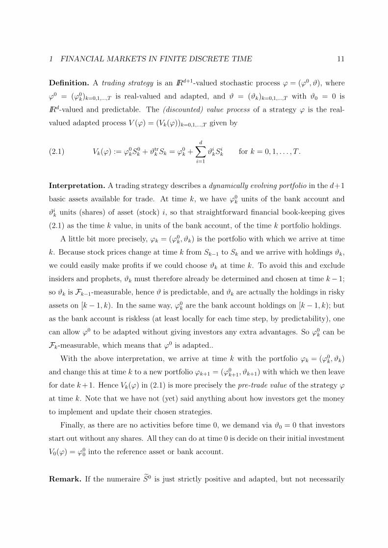
Definition. A trading strategy is an IRd+1-valued stochastic process ' = ('0
,#), where
'0 = ('0
k)k=0,1,...,T is real-valued and adapted, and # = (#k)k=0,1,...,T with #0 = 0 is
IRd-valued and predictable. The (discounted) value process of a strategy ' is the real-
valued adapted process V (') = (Vk('))k=0,1,...,T given by
(2.1) Vk(') := '0kS0k+ #
trkSk = '
0k+
dX
i=1
#i
kSi
kfor k = 0, 1, . . . , T .
Interpretation. A trading strategy describes a dynamically evolving portfolio in the d+1
basic assets available for trade. At time k, we have '0kunits of the bank account and
#i
kunits (shares) of asset (stock) i, so that straightforward financial book-keeping gives
(2.1) as the time k value, in units of the bank account, of the time k portfolio holdings.
A little bit more precisely, 'k = ('0k,#k) is the portfolio with which we arrive at time
k. Because stock prices change at time k from Sk�1 to Sk and we arrive with holdings #k,
we could easily make profits if we could choose #k at time k. To avoid this and exclude
insiders and prophets, #k must therefore already be determined and chosen at time k� 1;
so #k is Fk�1-measurable, hence # is predictable, and #k are actually the holdings in risky
assets on [k� 1, k). In the same way, '0kare the bank account holdings on [k� 1, k); but
as the bank account is riskless (at least locally for each time step, by predictability), one
can allow '0 to be adapted without giving investors any extra advantages. So '0
kcan be
Fk-measurable, which means that '0 is adapted..
With the above interpretation, we arrive at time k with the portfolio 'k = ('0k,#k)
and change this at time k to a new portfolio 'k+1 = ('0k+1,#k+1) with which we then leave
for date k+1. Hence Vk(') in (2.1) is more precisely the pre-trade value of the strategy '
at time k. Note that we have not (yet) said anything about how investors get the money
to implement and update their chosen strategies.
Finally, as there are no activities before time 0, we demand via #0 = 0 that investors
start out without any shares. All they can do at time 0 is decide on their initial investment
V0(') = '00 into the reference asset or bank account.
Remark. If the numeraire eS0 is just strictly positive and adapted, but not necessarily

1 FINANCIAL MARKETS IN FINITE DISCRETE TIME 12
predictable, then also '0 must be predictable. We shall see later in Proposition 2.3 that
this is automatically satisfied if the strategy ' is self-financing. ⇧
Of course, investors must do book-keeping about their expenses (and income). To
work out the costs associated to a trading strategy ' = ('0,#), we first observe that
apart from time 0, transactions only occur at the dates k when 'k is changed to 'k+1.
So the incremental cost for ' over the time interval (k, k + 1] occurs at time k when we
change from 'k to 'k+1 at the time-k prices Sk, and it is given by
�Ck+1(') := Ck+1(')� Ck(')(2.2)
= ('0k+1 � '
0k)S0
k+ (#k+1 � #k)
trSk
= '0k+1 � '
0k+
dX
i=1
(#i
k+1 � #i
k)Si
k.
Note that this is again in units of the bank account, hence discounted; and note also that
(2.2) is just a book-keeping identity with no room for alternative or artificial definitions.
Finally, the initial cost for ' at time 0 comes from putting '00 into the bank account; so
(2.3) C0(') = '00 = V0(').
We also point out that it is to some extent arbitrary whether we associate the above cost
increment �Ck+1(') to the time interval (k, k + 1] or to [k, k + 1). The choice we have
made simplifies notations, but is not financially compelling.
Remark. '0, # and S are all stochastic processes, and so '0k+1, '
0k, #k+1, #k and Sk are
all random variables, i.e., functions on ⌦ (to IR or IRd). In consequence, the equality in
(2.2) is really an equality between functions, and so (2.2) means that we have this equality
whenever we plug in an argument, i.e. for all !. In particular, what looks like one simple
equation is in fact an entire system of equations.
Of course, this comment applies not only to (2.2), but to all equalities or inequalities
between random variables. In addition, it is usually enough if the set of all ! for which
the relevant equality or inequality holds has probability 1; so e.g. (2.2) only needs to
1 FINANCIAL MARKETS IN FINITE DISCRETE TIME 13
hold P -a.s., and a similar comment applies again in general. We often do not write
P -a.s. explicitly unless this becomes important for some reason. ⇧
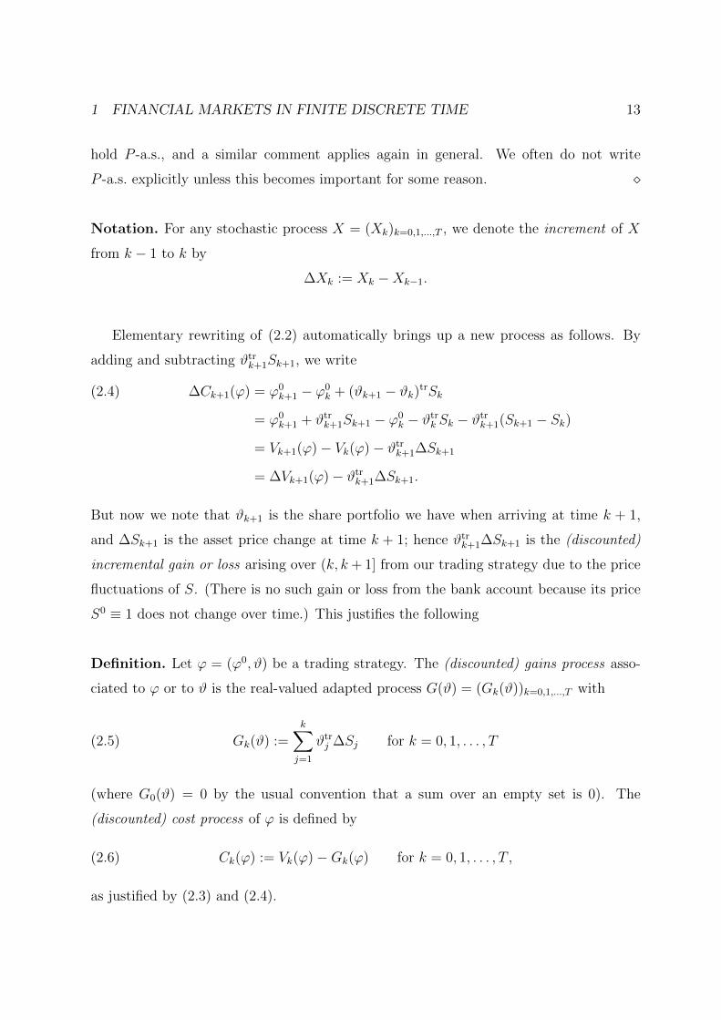
Notation. For any stochastic process X = (Xk)k=0,1,...,T , we denote the increment of X
from k � 1 to k by
�Xk := Xk �Xk�1.
Elementary rewriting of (2.2) automatically brings up a new process as follows. By
adding and subtracting #trk+1Sk+1, we write
�Ck+1(') = '0k+1 � '
0k+ (#k+1 � #k)
trSk(2.4)
= '0k+1 + #
trk+1Sk+1 � '
0k� #
trkSk � #
trk+1(Sk+1 � Sk)
= Vk+1(')� Vk(')� #trk+1�Sk+1
= �Vk+1(')� #trk+1�Sk+1.
But now we note that #k+1 is the share portfolio we have when arriving at time k + 1,
and �Sk+1 is the asset price change at time k + 1; hence #trk+1�Sk+1 is the (discounted)
incremental gain or loss arising over (k, k+ 1] from our trading strategy due to the price
fluctuations of S. (There is no such gain or loss from the bank account because its price
S0⌘ 1 does not change over time.) This justifies the following
Definition. Let ' = ('0,#) be a trading strategy. The (discounted) gains process asso-
ciated to ' or to # is the real-valued adapted process G(#) = (Gk(#))k=0,1,...,T with
(2.5) Gk(#) :=kX
j=1
#trj�Sj for k = 0, 1, . . . , T
(where G0(#) = 0 by the usual convention that a sum over an empty set is 0). The
(discounted) cost process of ' is defined by
(2.6) Ck(') := Vk(')�Gk(') for k = 0, 1, . . . , T ,
as justified by (2.3) and (2.4).

1 FINANCIAL MARKETS IN FINITE DISCRETE TIME 14
Remark 2.2. If we think of a continuous-time model where successive trading dates are
infinitely close together, then the increment �S in (2.5) becomes a di↵erential dS and
the sum becomes an integral. This explains why the stochastic integral G(#) =R# dS
provides the natural description of gains from trade in a continuous-time financial market
model. As a mathematical aside, we also note that we should think of this stochastic
integral as “G(#) =R P
d
i=1 #i dSi ”, not as “
Pd
i=1
R#i dSi ”. It turns out in stochastic
calculus that this does make a di↵erence. ⇧
By construction, Ck(') = C0(')+P
k
j=1 �Cj(') describes the cumulative (total) costs
for the strategy ' on the time interval [0, k]. If we do not want to worry about how to pay
these costs, we ideally try to make sure they never occur, by imposing this as a condition
on '. This motivates the next definition.
Definition. A trading strategy ' = ('0,#) is called self-financing if its cost process C(')
is constant over time (and hence equal to C0(') = V0(') = '00).
Due to (2.2), a strategy is self-financing if and only if it satisfies for each k
(2.7) '0k+1 � '
0k+ (#k+1 � #k)
trSk = �Ck+1(') = 0 P -a.s.
As it should, from economic intuition, this means that changing the portfolio from 'k
to 'k+1 at time k can be done cost-neutrally, i.e. with zero gains or losses at that time.
In particular, all losses from the portfolio due to stock price changes must be fully com-
pensated by gains from the bank account holdings and vice versa, without infusing or
draining extra funds. Due to (2.6), another equivalent description of a self-financing
strategy ' = ('0,#) is that it satisfies C(') = C0(') or
(2.8) V (') = V0(') +G(#) = '00 +G(#)
(in the sense that Vk(') = V0(')+Gk(#) P -a.s. for each k). This gives the following very
useful result.

1 FINANCIAL MARKETS IN FINITE DISCRETE TIME 15
Proposition 2.3. Any self-financing trading strategy ' = ('0,#) is uniquely determined
by its initial wealth V0 and its “risky asset component” #. In particular, any pair (V0,#),
where V0 is an F0-measurable random variable and # is an IRd-valued predictable process
with #0 = 0, specifies in a unique way a self-financing strategy. We sometimes write
' b= (V0,#) for the resulting strategy '.
Moreover, if ' = ('0,#) is self-financing, then ('0
k)k=1,...,T is automatically predictable.
The important feature of Proposition 2.3 is that it allows us to describe self-financing
strategies in a very simple way. We just have to specify the initial wealth V0 and the
strategy # we use for the risky assets; then the self-financing condition automatically
tells us how the bank account component '0 must evolve. The proof simply makes that
intuition precise, and so we give the short argument to get some practice.
Proof of Proposition 2.3. By (2.8) (or directly from the definitions of self-financing
and of C(') in (2.6), a strategy ' is self-financing if and only if for each k,
Vk(') = V0(') +Gk(#) P -a.s.
Because Vk(') = '0k+#tr
kSk by definition, we can rewrite the above equation for '0
kto get
'0k= V0(') +Gk(#)� #
trkSk,
which already shows that '0 is determined from V0 and # by the self-financing condition.
To see that '0 is predictable, we note that
Gk(#)�Gk�1(#) = �Gk(#) = #trk�Sk = #
trk(Sk � Sk�1).
Therefore
'0k= V0(') +Gk�1(#) +�Gk(#)� #
trkSk
= V0(') +Gk�1(#)� #trkSk�1
is directly seen to be Fk�1-measurable, because G(#) and S are adapted and # is pre-
dictable. q.e.d.

1 FINANCIAL MARKETS IN FINITE DISCRETE TIME 16
Remarks. 1) The notion of a strategy being self-financing is a kind of economic budget
constraint . Exactly like the cost process, this is formulated via basic financial book-
keeping requirements, and hence there cannot be any alternative (di↵erent) definitions
that make sense financially. This is a clear example where basic modelling sense must
override mathematical convenience. (In fact, there have been some attempts in continuous
time to use a di↵erent concept of stochastic integral, the so-called Wick integral, to define
the notion of a self-financing strategy. This has led to mathematical results which were
easier to derive; but the approach has subsequently been demonstrated to be economically
meaningless.)
2) We have expressed all prices and values in units of the bank account. However, as
basic intuition suggests, this has no e↵ect on whether or not a strategy is self-financing;
indeed, because eS0k> 0, (2.7) is equivalent to
(2.9) ('0k+1 � '
0k)eS0
k+ (#k+1 � #k)
tr eSk = 0
if we recall that S = eS/eS0. But (2.9) is clearly the self-financing condition expressed in
terms of the original units. The same argument shows that the notion of self-financing
is numeraire-invariant in the sense that it does not depend on the units in which we do
calculations. [! Exercise] Note that it also does not matter here whether eS0 is predictable
or only adapted. ⇧
Example (Stopping a process at a random time). Let ⌧ : ⌦ ! {0, 1, . . . , T} be
some mapping to be thought of as some random time; one specific example might be the
first time that stock i’s price exceeds that of stock j. We should like to use the “strategy”
to “buy and then hold until time ⌧”, because we believe for some reason that this might
be a good idea. For ease of notation, we take d = 1 so that there is just one risky asset.
Formally, let us take V0 := S0 and
#k(!) := I{k⌧(!)} =
8<
:1 for k = 1, . . . , ⌧(!)
0 for k = ⌧(!) + 1, . . . , T ,
which means exactly that we hold one unit of S up to and including time ⌧(!), but no
further. The value process of the corresponding self-financing “strategy” ' b= (V0,#) is

1 FINANCIAL MARKETS IN FINITE DISCRETE TIME 17
then by (2.8) and (2.5) given by
Vk(') = V0 +Gk(#)
= S0 +kX
j=1
#j�Sj
= S0 +kX
j=1
I{j⌧}(Sj � Sj�1)
= S0 +
8<
:Sk � S0 if ⌧ > k
S⌧ � S0 if ⌧ k
= Sk^⌧ =
8<
:Sk if k < ⌧
S⌧ if k � ⌧ ,
where we use the standard notation a ^ b := min(a, b).
The “stochastic process” S⌧ = (S⌧
k)k=0,1,...,T defined by
S⌧
k(!) := Sk^⌧ (!) := Sk^⌧(!)(!)
is called the process S stopped at ⌧ , because it clearly behaves like S up to time ⌧ and
remains constant after time ⌧ . Of course, for every ! 2 ⌦, this operation and notation
per se make sense for any stochastic process and any “random time” ⌧ as above.
However, a closer look shows that one must be a little more careful. For one thing, S⌧
could fail to be a stochastic process because S⌧
k= Sk^⌧ could fail to be a random variable,
i.e. could fail to be measurable. But (in discrete time like here) this is not a problem if
we assume that ⌧ is measurable, which is mild and reasonable enough.
While the measurability question is mainly technical, there is a second and financially
much more relevant issue. For ' to be a strategy, we need # to be predictable, and this
translates into the equivalent requirement that ⌧ should be a so-called stopping time,
meaning that ⌧ : ⌦ ! {0, 1, . . . , T} satisfies
(2.10) {⌧ j} 2 Fj for all j.
To see this, note that #k = I{k⌧} is Fk�1-measurable if and only if {⌧ � k} 2 Fk�1, and
to have this for all k is equivalent to (2.10) by passing to complements. By definition,

1 FINANCIAL MARKETS IN FINITE DISCRETE TIME 18
(2.10) means that ⌧ is a stopping time (with respect to IF , to be accurate). Intuitively,
(2.10) says that at each time j, we can observe from the then available information Fj
whether or not ⌧ is already past, i.e., whether the event corresponding to ⌧ has already
occurred. Typical examples are the first (or, by induction, n-th) time that an adapted
process does something that only involves looking at the past, e.g.
⌧(!) := inf{k : Si
k(!) > S
j
k(!)} ^ T
(the first time that stock i’s price exceeds that of stock j) or
⌧0(!) := inf
nk : S1
k(!) � 10 max
j=0,1,...,k�1S1j(!)o^ T
(the first time that stock 1’s price goes above ten times its past maximum value). On the
other hand, times looking at the future like
⌧00(!) := sup{k : S`
k(!) > 5} _ 0
(the last time that stock `’s price exceeds 5) are typically not stopping times; so they
cannot be used for constructing such buy-and-hold strategies. This makes intuitive sense.
Example (A doubling strategy). Suppose we have a model where the stock price can
in each step only go up or down. A well-known idea for a strategy to force winnings is
then to bet on a rise and keep on betting, doubling the stakes at each date, until the rise
occurs.
More formally, consider the binomial model with parameters u > 0, �1 < d < 0 and
r = 0; so the stock price Sk is either (1+u)Sk�1 or (1+d)Sk�1. To simplify computations,
suppose u = �d so that the growth factors Yk = Sk/Sk�1 are symmetric around 1. Note
that as seen earlier,
(2.11) �Sk = Sk � Sk�1 = Sk�1(Yk � 1).
Now denote by
(2.12) ⌧ := inf{k : Yk = 1 + u} ^ T

1 FINANCIAL MARKETS IN FINITE DISCRETE TIME 19
the (random) time of the first stock price rise and define
(2.13) #k :=1
Sk�12k�1
I{k⌧}.
Then ⌧ is a stopping time, because
{⌧ j} = {max(Y1, . . . , Yj) � 1 + u} 2 Fj
for each j, and so # is predictable because each #k is Fk�1-measurable. Note that this
uses {k ⌧} = {⌧ < k}c = {⌧ k � 1}c. Moreover,
#k+1Sk = 2kI{⌧�k+1} = 2⇥ 2k�1(I{⌧�k} � I{⌧=k}) = 2#kSk�1 � 2kI{⌧=k}
shows that while we are not successful, the value of our stock holdings (not the amount
of shares of the strategy itself) indeed doubles from one step to the next.
For V0 := 0, we now take the self-financing strategy ' corresponding to (V0,#). Its
value process is by (2.8) and (2.5) given by
Vk(') = Gk(#) =kX
j=1
#j�Sj =kX
j=1
2j�1I{j⌧}(Yj � 1),
using (2.11) and (2.13). By the definition (2.12) of ⌧ , we have Yj = 1 + d for j < ⌧ and
Yj = 1 + u for j = ⌧ ; so
Vk(') = I{⌧>k}
kX
j=1
2j�1d+ I{⌧k}
✓ ⌧�1X
j=1
2j�1d+ 2⌧�1
u
◆
= (2k � 1)d I{⌧>k} +�(2⌧�1
� 1)d+ 2⌧�1u�I{⌧k}.
Because u = �d and d < 0, we can write this as
Vk(') = |d|I{⌧k} � |d|(2k � 1)I{⌧>k},
which says that we obtain a value, and hence net gain, of |d| in all the (usually many)
cases that S goes up at least once up to time k, and make a (big) loss of |d|(2k � 1) in
the (hopefully unlikely) event that S always goes down up to time k.

1 FINANCIAL MARKETS IN FINITE DISCRETE TIME 20
One problem with the doubling strategy in the above example is that while it does
produce a gain in many cases, its value process goes very far below 0 in those cases where
“things go badly”. In continuous time or over an infinite time horizon, one obtains quite
pathological e↵ects if one does not forbid such strategies in some way. The next definition
aims at that.
Definition. For a � 0, a trading strategy ' is called a-admissible if its value process V (')
is uniformly bounded from below by �a, i.e. V (') � �a in the sense that Vk(') � �a
P -a.s. for all k. A trading strategy is admissible if it is a-admissible for some a � 0.
Interpretation. An admissible strategy has some credit line which imposes a lower bound
on the associated value process; so one may make debts, but only within clearly defined
limits. Note that while every admissible strategy has some credit line, the level of that
can be di↵erent for di↵erent strategies.
Remarks. 1) If ⌦ (or more generally F) is finite, any random variable can only take
finitely many values; for any model with finite discrete time, every trading strategy is
then admissible. But if F (or the time horizon) is infinite or time is continuous, imposing
admissibility is usually a genuine and important restriction. We return to this point later.
2) Note that all our prices and values are discounted and hence expressed in units of the
reference asset 0. Imposing a constant lower bound on a value process like admissibility
does is therefore obviously not invariant if we change to a di↵erent reference asset for
discounting. This is the root of the pitfalls mentioned earlier in Remark 2.1. ⇧
1 FINANCIAL MARKETS IN FINITE DISCRETE TIME 21
1.3 Some important martingale results
Martingales are ubiquitous in mathematical finance, as we shall see very soon. This
section collects a number of important facts and results we shall use later on.
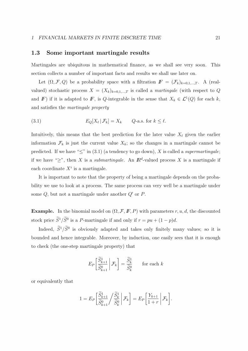
Let (⌦,F , Q) be a probability space with a filtration IF = (Fk)k=0,1,...,T . A (real-
valued) stochastic process X = (Xk)k=0,1,...,T is called a martingale (with respect to Q
and IF ) if it is adapted to IF , is Q-integrable in the sense that Xk 2 L1(Q) for each k,
and satisfies the martingale property
(3.1) EQ[X` | Fk] = Xk Q-a.s. for k `.
Intuitively, this means that the best prediction for the later value X` given the earlier
information Fk is just the current value Xk; so the changes in a martingale cannot be
predicted. If we have “” in (3.1) (a tendency to go down), X is called a supermartingale;
if we have “�”, then X is a submartingale. An IRd-valued process X is a martingale if
each coordinate Xi is a martingale.
It is important to note that the property of being a martingale depends on the proba-
bility we use to look at a process. The same process can very well be a martingale under
some Q, but not a martingale under another Q0 or P .
Example. In the binomial model on (⌦,F , IF, P ) with parameters r, u, d, the discounted
stock price eS1/eS0 is a P -martingale if and only if r = pu+ (1� p)d.
Indeed, eS1/eS0 is obviously adapted and takes only finitely many values; so it is
bounded and hence integrable. Moreover, by induction, one easily sees that it is enough
to check (the one-step martingale property) that
EP
eS1k+1
eS0k+1
����Fk
�=eS1k
eS0k
for each k
or equivalently that
1 = EP
eS1k+1
eS0k+1
�eS1k
eS0k
����Fk
�= EP
Yk+1
1 + r
����Fk
�.

1 FINANCIAL MARKETS IN FINITE DISCRETE TIME 22
But Yk+1 is independent of Fk and takes the values 1+u, 1+ d with probabilities p, 1� p.
Therefore
EP
Yk+1
1 + r
����Fk
�=
1
1 + rEP [Yk+1]
=1
1 + r
�p(1 + u) + (1� p)(1 + d)
�
=1 + pu+ (1� p)d
1 + r.
This equals 1 if and only if r = pu+ (1� p)d, which proves the assertion.
For mathematical reasons and arguments, the following generalisation of martingales
is extremely useful.
Definition. An adapted process X = (Xk)k=0,1,...,T null at 0 (i.e. with X0 = 0) is
called a local martingale (with respect to Q and IF ) if there exists a sequence of stop-
ping times (⌧n)n2IN increasing to T such that for each n 2 IN , the stopped process
X⌧n = (Xk^⌧n)k=0,1,...,T is a (Q, IF )-martingale. We then call (⌧n)n2IN a localising sequence.
Remarks. 1) Especially in continuous time, local martingales can be substantially
di↵erent from (true) martingales; the concept is rather subtle.
2) In parts of the recent finance literature, local martingales have come up in studies
of price bubbles. ⇧
The next result gives a whole class of examples of local martingales.
Theorem 3.1. Suppose X = (Xk)k=0,1,...,T is an IRd-valued martingale or local martingale
null at 0. For any IRd-valued predictable process #, the stochastic integral process # X
defined by
# Xk :=kX
j=1
#trj�Xj for k = 0, 1, . . . , T

1 FINANCIAL MARKETS IN FINITE DISCRETE TIME 23
is then a (real-valued) local martingale null at 0. If X is a martingale and # is bounded,
then # X is even a martingale.
Note that if we think of X = S as discounted asset prices, then # S = G(#) is the
discounted gains process of the self-financing strategy ' b= (0,#).
Proof of Theorem 3.1. This result is important enough to deserve at least a partial
proof. So suppose X is a Q-martingale and # is bounded. Then # X is also Q-integrable,
it is always adapted, and
EQ[# Xk+1 � # Xk | Fk] = EQ[#trk+1�Xk+1 | Fk]
=dX
i=1
EQ[#i
k+1�Xi
k+1 | Fk].
But #i
k+1 is bounded and Fk-measurable because # is predictable, and �Xi
k+1 is Q-inte-
grable because X is a Q-martingale; so
EQ[#i
k+1�Xi
k+1 | Fk] = #i
k+1EQ[�Xi
k+1 | Fk] = 0
again because Xi is a Q-martingale. So # X also has the martingale property.
For the mathematicians: Because # is predictable,
�n := inf{k : |#k+1| > n} ^ T
is a stopping time, and |#k| n for k �n by definition. So if (⌧n)n2IN is a localising
sequence for X, one can easily check with the above argument that ⌧ 0n:= ⌧n ^ �n yields a
localising sequence for # X. This gives the general result. q.e.d.
We have seen earlier that if ⌧ is any stopping time, then #k := I{k⌧} is predictable,
and of course bounded. So if we note that # X = X⌧�X0, an immediate consequence
of Theorem 3.1 is
Corollary 3.2. For any martingale X and any stopping time ⌧ , the stopped process X⌧
is again a martingale. In particular, EQ[Xk^⌧ ] = EQ[X0] for all k.

1 FINANCIAL MARKETS IN FINITE DISCRETE TIME 24
Interpretation. A martingale describes a fair game in the sense that one cannot predict
where it goes next. Corollary 3.2 says that one cannot change this fundamental character
by cleverly stopping the game — and Theorem 3.1 says that as long as one can only use
information from the past, not even complicated clever betting (in the form of trading
strategies) will help.
Remark. Corollary 3.2 still holds if we replace “martingale” by either “supermartingale”
or “submartingale”. However, such a generalisation is not true in general for Theorem 3.1.
[! Exercise] ⇧
In general, the stochastic integral with respect to a local martingale is only a local
martingale — and in continuous time, it may fail to be even that in the most general
case. But there is one situation where things are very nice in discrete time, and this is
tailor-made for applications in mathematical finance, as one can see by looking at the
definition of self-financing and admissible strategies.
Theorem 3.3. Suppose that X is an IRd-valued local Q-martingale null at 0 and # is
an IRd-valued predictable process. If the stochastic integral process # X is uniformly
bounded below (i.e. # Xk � �b Q-a.s. for all k, with a constant b � 0), then # X is a
Q-martingale.
Proof. See Follmer/Schied [9, Theorem 5.15]. A bit more generally, this relies on
the result that in discrete (possibly infinite) time, a local martingale that is uniformly
bounded below is a true martingale. More precisely: If L = (Lk)k2IN0 is a local Q-martin-
gale with EQ[|L0|] < 1 and T 2 IN is such that EQ[L�T] < 1, then the stopped process
LT = (Lk)k=0,1,...,T is a Q-martingale. q.e.d.
We shall see later that Theorem 3.3 is extremely useful.
Remark. We have formulated everything here for the setting k = 0, 1, . . . , T of finite

1 FINANCIAL MARKETS IN FINITE DISCRETE TIME 25
discrete time. The same definitions and results also apply for the setting k 2 IN0 of
infinite discrete time; the only required change is that one must replace T by 1 in an
appropriate manner. ⇧

1 FINANCIAL MARKETS IN FINITE DISCRETE TIME 26
1.4 An example: The multinomial model
In this section, we take a closer look at the multinomial model already introduced briefly
in Section 1.1. Recall that this is the multiplicative model with i.i.d. returns given by
eS0k
eS0k�1
= 1 + r > 0 for all k,
eS1k
eS1k�1
= Yk for all k,
where eS00 = 1, eS1
0 = S10 > 0 is a constant, and Y1, . . . , YT are i.i.d. and take the finitely
many values 1 + y1, . . . , 1 + ym with respective probabilities p1, . . . , pm. To avoid degen-
eracies and fix the notation, we assume that all the probabilities pj are > 0 and that
ym > ym�1 > · · · > y1 > �1. This also ensures that eS1 remains strictly positive.
The interpretation for this model is very simple. At each step, the bank account
changes by a factor of 1+r, while the stock changes by a random factor that can only take
the m di↵erent values 1+yj, j = 1, . . . ,m. The choice of these factors happens randomly,
with the same mechanism (identically distributed) at each date, and independently across
dates. Intuition suggests that for a reasonable model, the sure factor 1 + r should lie
between the minimal and maximal values 1 + y1 and 1 + ym of the (uncertain) random
factor; we come back to this issue in the next chapter when we discuss absence of arbitrage.
The simplest and in fact canonical model for this setup is a path space. Let
⌦ = {1, . . . ,m}T
=�! = (x1, . . . , xT ) : xk 2 {1, . . . ,m} for k = 1, . . . , T
be the set of all strings of length T formed by elements of {1, . . . ,m}. Take F = 2⌦, the
family of all subsets of ⌦, and define P by setting
(4.1) P [{!}] = px1px2 · · · pxT =TY
k=1
pxk.
Finally, define Y1, . . . , YT by
(4.2) Yk(!) := 1 + yxk

1 FINANCIAL MARKETS IN FINITE DISCRETE TIME 27
so that Yk(!) = 1 + yj if and only if xk = j. This mathematically formalises the idea
that at each step k, we choose the value 1 + yj for Yk with probability pj, and we do this
independently over k because P is obtained by multiplication. A nice way to graphically
illustrate the construction of this canonical model (⌦,F , P ) is to draw a (non-recombining)
tree of length T with m branches going out from each node. We then place the pj as
one-step transition probabilities into each branching, and the probability of each single
trajectory ! is obtained by multiplying the one-step transition probabilities along the
way. [A figure to illustrate this is very helpful.]
As usual, we take as filtration the one generated by eS1 (or, equivalently, by Y ) so that
Fk = �(Y1, . . . , Yk) for k = 0, 1, . . . , T .
Intuitively , this means that up to time k, we can observe the values of Y1, . . . , Yk and
hence the first k “bits” of the trajectory or string !. Formally , this translates as follows.
Recall that for a general probability space (⌦,F , P ), a set B is an atom of a �-field
G ✓ F if B 2 G, P [B] > 0 and any C 2 G with C ✓ B has either P [C] = 0 or
P [C] = P [B]. In that sense, atoms of a �-field G are minimal elements of G, where
minimal is measured with the help of P .
In the above path-space setting, the only set of probability zero is the empty set, and
so P [C] = 0 and P [C] = P [B| translate into C = ; and C = B, respectively. A set
A ✓ ⌦ is therefore an atom of Fk if and only if there exists a string (x1, . . . , xk) of length
k with elements xi 2 {1, . . . ,m} such that A consists of all those ! 2 ⌦ that start with
the substring (x1, . . . , xk), i.e.
A = Ax1,...,xk:=�! = (x1, . . . , xT ) 2 {1, . . . ,m}
T : xi = xi for i = 1, . . . , k .
This has the following consequences for our path-space model:
– Each Fk is parametrised by substrings of length k and therefore contains precisely
mk atoms.
– When going from time k to time k + 1, each atom A = Ax1,...,xkfrom Fk splits into
precisely m subsets A1 = Ax1,...,xk,1, . . . , Am = Ax1,...,xk,mthat are atoms of Fk+1. So

1 FINANCIAL MARKETS IN FINITE DISCRETE TIME 28
we can see very precisely and graphically how information about the past, i.e. the
initial part of trajectories !, is growing and refining over time.
It is clear from the above description that for any k, the atoms of Fk are pairwise disjoint
and their union is ⌦; in other words, the atoms of Fk form a partition of ⌦ so that we
can write
⌦ =[
(x1,...,xk)2{1,...,m}kAx1,...,xk
with the Ax1,...,xkpairwise disjoint.
Finally, each set B in Fk is a union of atoms of Fk; so the family Fk of events observable
up to time k consists of 2mksets (because for each of the mk atoms, we can either include
it or not when forming B).
Remark. For many (but not all) purposes in the multinomial model, it is enough if one
looks at time k only at the current value eS1kof the stock. In graphical terms, this means
that one makes the underlying tree recombining by collapsing at each time k into one
(big) node all those nodes where eS1khas the same value. In terms of �-fields, this amounts
to looking at time k only at Gk = �(eS1k). It is clear that Gk (as a collection of subsets
of ⌦, i.e. Gk ✓ 2⌦) is substantially smaller than Fk and also that the recombining tree
is much less complicated. However, note that the family (Gk)k=0,1,...,T is in general not a
filtration; we do not have Gk ✓ G` for k `. ⇧
With the help of the atoms introduced above, we can also give a very precise and
intuitive description of all probability measures Q on FT . First of all, we identify each atom
in Fk with a node at time k of the non-recombining tree, namely that node which is reached
via the substring (x1, . . . , xk) that parametrises the atom. For any atom A = Ax1,...,xkof
Fk, we then look at its m successor atoms A1 = Ax1,...,xk,1, . . . , Am = Ax1,...,xk,mof Fk+1,
and we define the one-step transition probabilities for Q at the node corresponding to A
by the conditional probabilities (note that Aj \ A = Aj as Aj ✓ A)
(4.3) Q[Aj |A] =Q[Aj]
Q[A]for j = 1, . . . ,m.

1 FINANCIAL MARKETS IN FINITE DISCRETE TIME 29
Because A is the disjoint union of A1, . . . , Am, we have 0 Q[Aj |A] 1 for j = 1, . . . ,m
andP
m
j=1 Q[Aj |A] = 1. (If Q[A] is zero, then so are all the Q[Aj] because Aj ✓ A, and
we can for instance define the ratios to be 1m, to make sure they are � 0 and sum to 1.)
By attaching all these one-step transition probabilities to each branch from each node, we
then have by construction a decomposition or factorisation of Q in such a way that for
every trajectory ! 2 ⌦, its probability Q[{!}] is the product of the successive one-step
transition probabilities along !. This follows in an elementary way from the definition of
conditional probabilities, Q[C \D] = Q[C]Q[D |C], and by iteration. In more detail, we
can write, for ! = (x1, . . . , xT ),
Q[{!}] = Q[Ax1,...,xT ]
= Q[Ax1,...,xT |Ax1,...,xT�1 ]Q[Ax1,...,xT�1 ]
= qxT (x1, . . . , xT�1)Q[Ax1,...,xT�1 ]
and iterate from here to obtain
Q[{!}] = qx1
T�1Y
j=1
qxj+1(x1, . . . , xj).
In the above procedure, we have factorised a given probability measure Q on (⌦,F)
into its one-step transition probabilities. However, this idea also works the other way
round. If we take for each node m numbers in [0, 1] that sum to 1 and attach them to the
branches from that node as “one-step transition probabilities”, then defining Q[{!}] for
each ! 2 ⌦ to be as in (4.1) the product of the numbers along ! defines a probability mea-
sure Q on FT whose one-step transition probabilities, defined as above in (4.3) via atoms,
coincide with the a priori chosen numbers at each node. Indeed, just using (4.1) gives in
(4.3) that Q[Aj |A] = Q[Ax1,...,xk,j|Ax1,...,xk
] = qj(x1, . . . , xk). Hence we can describe Q
equivalently either via its global weights Q[{!}] or via its local transition behaviour. The
latter description is particularly useful when computing conditional expectations under
Q, as we shall see later in Sections 2.1, 2.3 or 3.3.
For a general Q, one can have di↵erent one-step transition probabilities at every node
in the tree. The (coordinate) variables Y1, . . . , YT from (4.2) are independent under Q if
and only if for each k, the one-step transition probabilities are the same for each node at

1 FINANCIAL MARKETS IN FINITE DISCRETE TIME 30
time k (but they can still di↵er across dates k). Finally, Y1, . . . , YT are i.i.d. under Q if
and only if at each node throughout the tree, the one-step transition probabilities are the
same. Probability measures with this particular structure can therefore be described by
m � 1 parameters; recall that the m one-step transition probabilities at any given node
must sum to 1, which eliminates one degree of freedom.
Remark. We have discussed the path space formulation for the multinomial model where
each node in the tree has the same number of successor nodes and in that sense is homo-
geneous in time. But of course, the same considerations can be done for any model where
the final �-algebra FT is finite. The only di↵erence is that the corresponding event tree
is no longer nicely symmetric and homogeneous, which makes the notation (but not the
basic considerations) more complicated. ⇧

2 ARBITRAGE AND MARTINGALE MEASURES 31
2 Arbitrage and martingale measures
Our goal in this chapter is to formalise the idea that a reasonable financial market model
should not allow the construction of riskless yet profitable investment strategies, and to
characterise this by an equivalent mathematical property. Throughout the chapter,
we consider a discounted financial market in finite discrete time on (⌦,F , IF, P ) with
IF = (Fk)k=0,1,...,T , where discounted asset prices are given by the processes S0⌘ 1 and
S = (Sk)k=0,1,...,T , the latter taking values in IRd.
2.1 Arbitrage
Recall from Proposition 1.2.3 that any pair (V0,#) consisting of V0 2 L0(F0) and an
IRd-valued IF -predictable process # can be identified with a self-financing strategy ',
whose value process is then given by V (') = V0 + G(#) = V0 +R# dS = V (V0,#). We
shortly write ' b= (V0,#). (Of course, we work throughout in units of asset 0.) Hence
G(#) = V (0,#) describes the cumulative gains or losses one can generate from initial
capital 0 through self-financing trading via ' b= (0,#). We also recall that a strategy '
is a-admissible if V (') � �a, and admissible if it is a-admissible for some a � 0. Note
that these notions depend on the chosen accounting unit or numeraire (here S0), except
for 0-admissibility.
Definition. An arbitrage opportunity is an admissible self-financing strategy ' b= (0,#)
with zero initial wealth, with VT (') � 0 P -a.s. and with P [VT (') > 0] > 0. The finan-
cial market (⌦,F , IF, P, S0⌘ 1, S) or shortly S is called arbitrage-free if there exist no
arbitrage opportunities. Sometimes one also says that S satisfies (NA).
Interpretation. An arbitrage opportunity produces something (nonnegative final wealth
VT (') � 0, with a genuine chance of having strictly positive final wealth) out of noth-
ing (zero initial capital) without any risk (because the strategy is self-financing). In a
well-functioning market, such “money pumps” cannot exist (for long) because they would
quickly be exploited and hence would vanish. So absence of arbitrage is a natural eco-
2 ARBITRAGE AND MARTINGALE MEASURES 32
nomic/financial requirement for a reasonable model of a financial market.
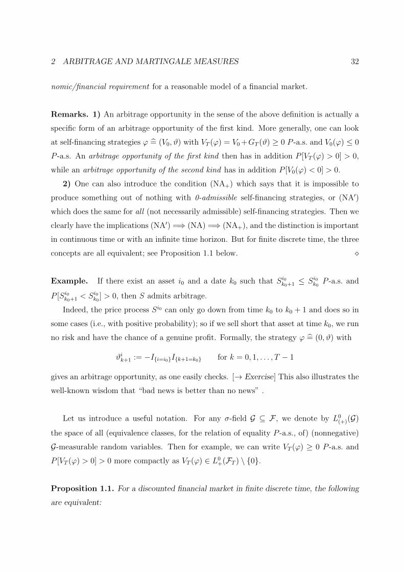
Remarks. 1) An arbitrage opportunity in the sense of the above definition is actually a
specific form of an arbitrage opportunity of the first kind. More generally, one can look
at self-financing strategies ' b= (V0,#) with VT (') = V0+GT (#) � 0 P -a.s. and V0(') 0
P -a.s. An arbitrage opportunity of the first kind then has in addition P [VT (') > 0] > 0,
while an arbitrage opportunity of the second kind has in addition P [V0(') < 0] > 0.
2) One can also introduce the condition (NA+) which says that it is impossible to
produce something out of nothing with 0-admissible self-financing strategies, or (NA0)
which does the same for all (not necessarily admissible) self-financing strategies. Then we
clearly have the implications (NA0) =) (NA) =) (NA+), and the distinction is important
in continuous time or with an infinite time horizon. But for finite discrete time, the three
concepts are all equivalent; see Proposition 1.1 below. ⇧
Example. If there exist an asset i0 and a date k0 such that Si0k0+1 S
i0k0
P -a.s. and
P [Si0k0+1 < S
i0k0] > 0, then S admits arbitrage.
Indeed, the price process Si0 can only go down from time k0 to k0 + 1 and does so in
some cases (i.e., with positive probability); so if we sell short that asset at time k0, we run
no risk and have the chance of a genuine profit. Formally, the strategy ' b= (0,#) with
#i
k+1 := �I{i=i0}I{k+1=k0} for k = 0, 1, . . . , T � 1
gives an arbitrage opportunity, as one easily checks. [! Exercise] This also illustrates the
well-known wisdom that “bad news is better than no news” .
Let us introduce a useful notation. For any �-field G ✓ F , we denote by L0(+)(G)
the space of all (equivalence classes, for the relation of equality P -a.s., of) (nonnegative)
G-measurable random variables. Then for example, we can write VT (') � 0 P -a.s. and
P [VT (') > 0] > 0 more compactly as VT (') 2 L0+(FT ) \ {0}.
Proposition 1.1. For a discounted financial market in finite discrete time, the following
are equivalent:

2 ARBITRAGE AND MARTINGALE MEASURES 33
1) S is arbitrage-free.
2) There exists no self-financing strategy ' b= (0,#) with zero initial wealth and satis-
fying VT (') � 0 P -a.s. and P [VT (') > 0] > 0; in other words, S satisfies (NA0).
3) For every (not necessarily admissible) self-financing strategy ' with V0(') = 0 P -a.s.
and VT (') � 0 P -a.s., we have VT (') = 0 P -a.s.
4) For the space
G0 := {GT (#) : # is IRd-valued and predictable}
of all final wealths that one can generate from zero initial wealth through some
self-financing trading ' b= (0,#), we have
G0\ L
0+(FT ) = {0}.
Remarks. 1) Proposition 1.1 and its proof substantiate the above comment that all
three above formulations for absence of arbitrage are equivalent in finite discrete time.
2) The mathematical relevance of Proposition 1.1 is that it translates the no-arbitrage
condition (NA) into the formulation in 4) which has a very useful geometric interpretation.
We shall exploit this in the next section. ⇧
Proof of Proposition 1.1. “2) , 3)” is obvious, and “2) , 4)” is a direct consequence
of the parametrisation of self-financing strategies in Proposition 1.2.3. It is also clear that
(NA0) as in 2) implies (NA) as in 1). Finally, the argument for “1) ) 2)” is indirect
and even shows a bit more: We claim that if one has a self-financing strategy ' which
produces something out of nothing, one can construct from ' a 0-admissible self-financing
strategy ' which also produces something out of nothing. Indeed, if ' is not already
0-admissible itself, then the set Ak := {Vk(') < 0} has P [Ak] > 0 for some k. We take
as k0 the largest of these k and then define ' simply as the strategy ' on Ak0 after time
k0. In words, we wait until we can start on some set with a negative initial capital and
transform that via ' into something nonnegative. As this turns something nonpositive

2 ARBITRAGE AND MARTINGALE MEASURES 34
into something nonnegative and keeps wealth nonnegative by construction, it produces
the desired arbitrage opportunity.
(Writing out the above verbal argument in formal terms and checking all the details
is an excellent [! exercise] necessarily increase the financial understanding.) q.e.d.
Our next intermediate goal is to give a simple probabilistic condition that excludes
arbitrage opportunities. Recall that two probability measuresQ and P on F are equivalent
(on F), written as Q ⇡ P (on F), if they have the same nullsets (in F), i.e. if for each
set A (in F), we have P [A] = 0 if and only if Q[A] = 0. Intuitively, this means that while
P and Q may di↵er in their quantitative assessments, they qualitatively agree on what is
“possible or impossible”.
Example. If we construct the multinomial model as in Section 1.4 as an event tree on the
canonical path space ⌦ = {1, . . . ,m}T with F = 2⌦, then we know that any probability
measure on (⌦,F) can be described by its collection of one-step transition probabilities,
which all lie between 0 and 1, i.e. in [0, 1].
Now consider two probability measures P and Q on (⌦,F). If some of the transition
probabilities pij of P are 0 (or 1), a characterisation of Q being equivalent to P is a bit
involved, and so we assume (as for example in the multinomial model) that P [{!}] > 0
for all ! 2 ⌦. This means that all one-step transition probabilities pij for P lie in the open
interval (0, 1), and then we have Q ⇡ P if and only if all one-step transition probabilities
qij for Q lie in (0, 1) as well.
Now we go back to the general case.
Lemma 1.2. If there exists a probability measure Q ⇡ P on FT such that S is a
Q-martingale, then S is arbitrage-free.
Proof. If S is a Q-martingale and ' b= (0,#) is an admissible self-financing strategy,
then V (') = G(#) = # S is a stochastic integral of S and uniformly bounded below (by

2 ARBITRAGE AND MARTINGALE MEASURES 35
some �a with a � 0). By Theorem 1.3.3, V (') is thus also a Q-martingale and so
EQ[VT (')] = EQ[V0(')] = 0.
Now suppose in addition that Q ⇡ P on FT , so that Q-a.s. and P -a.s. are the same thing
for all events in FT . If ' b= (0,#) is an admissible self-financing strategy with VT (') � 0
P -a.s., then also VT (') � 0 Q-a.s. But EQ[VT (')] = 0 by the above argument, and so
we must have VT (') = 0 Q-a.s., hence also VT (') = 0 P -a.s. By Proposition 1.1, S is
therefore arbitrage-free. q.e.d.
Remark 1.3. 1) It would be enough if S is only a local Q-martingale, because we could
still use Theorem 1.3.3.
2) An alternative proof of Lemma 1.2 goes as follows. This is attractive because
it proves a more general result, and the proof still works (with one reference changed)
in continuous or infinite discrete time. Suppose that Q ⇡ P on FT is such that S is
a local Q-martingale and take an admissible self-financing strategy ' b= (0,#). Then
V (') = G(#) = # S is a local Q-martingale by Theorem 1.3.1, with V0(') = 0, and V (')
is bounded below because ' is admissible. (In continuous time, the argument and reference
here are bit di↵erent.) But then V (') is a Q-supermartingale (this is easily argued via
localising and passing to the limit with the help of Fatou’s lemma [! exercise]), and so we
get EQ[VT (')] EQ[V0(')] = 0. If in addition VT (') � 0 P -a.s., we also get VT (') � 0
Q-a.s., hence VT (') = 0 Q-a.s., and then also VT (') = 0 P -a.s. This allows us to conclude
as before.
3) We can also give a complete proof of Lemma 1.2 which relies only on proved
results. We still use that with ' b= (0,#), we have V (') = G(#) = # S. Now because
# is predictable, the process #(n) defined by #(n)k
:= #kI{|#k|n} is again predictable and
bounded. So if S is a martingale under Q, then #(n)S is again a Q-martingale by (the
simple and proved part of) Theorem 1.3.1. Moreover, the definition of #(n) yields
�(#(n)k
)tr�Sk = �#trk�SkI{|#k|n} �#
trk�SkI{#tr
k �Sk0}I{|#k|n} �#trk�SkI{#tr
k �Sk0}
so that ((#(n)k
)tr�Sk)� (#trk�Sk)� for all k and hence (#(n)
S)� (# S)�. But
V (') is bounded below by �a because ' is admissible, and therefore the entire sequence

2 ARBITRAGE AND MARTINGALE MEASURES 36
(G(#(n)))n2IN = (#(n)S)n2IN is also bounded below by �a. This allows us to use Fatou’s
lemma and conclude from the martingale property of each G(#(n)) that V (') = # S is a
Q-supermartingale; indeed,
EQ[Gk(#) | Fk�1] = EQ
hlimn!1
Gk(#(n))���Fk�1
i lim inf
n!1EQ[Gk(#
(n)) | Fk�1]
= lim infn!1
Gk�1(#(n)) = Gk�1(#).
Then we can finish the proof as before in 2).
4) In continuous time, Theorem 1.3.3 no longer holds; then it is useful and important
to have for proofs the alternative route via 2). Also for discrete but infinite time, one
must be careful about the behaviour at 1. ⇧
Example. Consider themultinomial model on the canonical path space ⌦ = {1, . . . ,m}T
and suppose as usual that P [{!}] > 0 for all ! 2 ⌦. (We can also assume that the returns
Y1, . . . , YT are i.i.d. under P , but this is actually not needed for the subsequent reasoning.)
To find Q ⇡ P such that S1 = eS1
/eS0 is a Q-martingale (recall that we always work in
units of asset 0), we need to find one-step transition probabilities in the open interval
(0, 1) such that
EQ[eS1k/eS0
k| Fk�1] = eS1
k�1/eS0k�1 for all k.
Because
eS1k/eS0
k
eS1k�1/
eS0k�1
=eS1k/eS1
k�1
eS0k/eS0
k�1
=Yk
1 + r,
we equivalently need EQ[Yk/(1 + r) | Fk�1] = 1 for all k.
Now fix k and look at a node corresponding to an atom A(k�1) = Ax1,...,xk�1
of Fk�1 at
time k�1 with corresponding one-step transition probabilities q1, . . . , qm. (We sometimes
omit to write the indices for qj = qj(A(k�1)) = qj(x1, . . . , xk�1), but of course the one-step
transition probabilities can depend on the atom A(k�1) and hence on the time k.) For
the associated probability measure Q, the quantities qj(A(k�1)) = Q[Yk = 1 + yj |A(k�1)]
for branch j = 1, . . . ,m then describe the (one-step) conditional distribution of Yk given
2 ARBITRAGE AND MARTINGALE MEASURES 37
Fk�1 at that node, and so
on the atom A(k�1), EQ[Yk | Fk�1] = EQ[Yk |A
(k�1)]
=mX
j=1
qj(A(k�1))(1 + yj)
= 1 +mX
j=1
qj(A(k�1))yj
which implies that
EQ[Yk | Fk�1] =X
atomsA(k�1)2Fk�1
IA(k�1)EQ[Yk |A
(k�1)]
= 1 +X
atomsA(k�1)2Fk�1
IA(k�1)qj(A
(k�1))yj,
and we want this to equal 1+r. Note that although we have started with a particular time
k and atom A(k�1), the resulting condition always looks the same; this is due to the ho-
mogeneity in the structure of the multinomial model. The above conditional expectation
equals 1 + r if and only if the equation
mX
j=1
qj(A(k�1))yj = r
has a solution q1(A(k�1)), . . . , qm(A(k�1)). Because we want all the qj(A(k�1)) to lie in
(0, 1) and because we have ym > ym�1 > · · · > y1 > �1 by the assumed labelling, this
can clearly be achieved if and only if ym > r > y1, i.e. if and only if the riskless interest
rate r for the bank account lies strictly between the smallest and largest return values,
y1 and ym, for the stock. Moreover, we can then choose the qj(A(k�1)) independently of k
and A(k�1), and if we do that, the corresponding probability measure Q has the property
that the returns Y1, . . . , YT are i.i.d. under Q. But we also see that there are clearly many
Q0⇡ P on FT such that eS1
/eS0 is a Q0-martingale, but Y1, . . . , YT are not i.i.d. under Q0.
In summary, we obtain the following result.

2 ARBITRAGE AND MARTINGALE MEASURES 38
Corollary 1.4. In the multinomial model with parameters y1 < · · · < ym and r, there
exists a probability measure Q ⇡ P such that eS1/eS0 is a Q-martingale if and only if
y1 < r < ym.
The interpretation of the condition y1 < r < ym is very intuitive. It says that in
comparison to the riskless bank account eS0, the stock eS1 has the potential for both
higher and lower growth than eS0. Hence eS1 is genuinely more risky than eS0. One has
the feeling that this should not only be su�cient to exclude arbitrage opportunities, but
necessary as well. That feeling is correct, as we shall see in the next section; alternatively,
one can also prove this directly. [! Exercise]
For the special case of the binomial model, we can even say a bit more.
Corollary 1.5. In the binomial model with parameters u > d and r, there exists a
probability measure Q ⇡ P such that eS1/eS0 is a Q-martingale if and only if u > r > d.
In that case, Q is unique (on FT ) and characterised by the property that Y1, . . . , YT are
i.i.d. under Q with parameter
Q[Yk = 1 + u] = q⇤ =
r � d
u� d= 1�Q[Yk = 1 + d].
Proof. The martingale conditionP
m
j=1 qj(A(k�1))yj = r reduces, with m = 2, y1 = d,
y2 = u and q := q2(A(k�1)), to the equation (1 � q)d + qu = r, which has the unique
solution q⇤. Because the one-step transition probabilities for Q are thus the same in each
node throughout the tree, the i.i.d. description under Q follows as in Section 1.4 and in
the preceding discussion. q.e.d.

2 ARBITRAGE AND MARTINGALE MEASURES 39
2.2 The fundamental theorem of asset pricing
We have already seen in Lemma 1.2 a su�cient condition for S to be arbitrage-free.
Moreover, the multinomial model has led us to suspect that this condition might be
necessary as well. In this section, we shall prove that this is indeed so, for every financial
market model in finite discrete time. To give the result a crisp formulation, we first
introduce a new and very important concept.
Definition. An equivalent (local) martingale measure (E(L)MM) for S is a probability
measure Q equivalent to P on FT such that S is a (local) Q-martingale. We denote by
IPe(S) or simply IPe the set of all EMMs for S and by IPe,loc the set of all ELMMs for S.
Clearly, IPe ✓ IPe,loc.
Saying that IPe(,loc)(S) is non-empty is the same as saying that there exists an equiv-
alent (local) martingale measure Q for S. By Lemma 1.2 and the discussion around it,
both these properties imply that S is arbitrage-free or, equivalently, that S satisfies (NA).
It is very remarkable and important that the converse implication holds as well.
Theorem 2.1 (Dalang/Morton/Willinger). Consider a (discounted) financial market
model in finite discrete time. Then S is arbitrage-free if and only if there exists an
equivalent martingale measure for S. In brief:
(NA) () IPe(S) 6= ; () IPe,loc(S) 6= ;.
This result deserves a number of comments :
1) The crucial significance of Theorem 2.1 is that it translates the economic/financial
condition of absence of arbitrage into an equivalent, purely mathematical/probabilistic
condition. This opens the door for the use of martingale theory, with its many tools and
results, for the study of financial market models.
2) The classical theorems in martingale theory on gambling say that one cannot win in
a systematic way if one bets on a martingale (see the stopping theorem or Doob’s systems

2 ARBITRAGE AND MARTINGALE MEASURES 40
theorem). Theorem 2.1 can be viewed as a converse; it says that if one cannot win by
betting on a given process, then that process must be a martingale — at least after an
equivalent change of probability measure.
3) Note that we make no integrability assumptions about S (under P ); so it is also
noteworthy that S, being a Q-martingale, is automatically integrable under (some) Q.
(To put this into perspective, one should add that it is a minor point; one can always
easily construct [! exercise] a probability measure R equivalent to P such that S becomes
under R as nicely integrable as one wants. But of course such an R will in general not be
a martingale measure for S.)
Proving Theorem 2.1 is not elementary if one wants to allow models where the under-
lying probability space (⌦,F , P ) is infinite, or more precisely if one of the �-fields Fk,
k T , is infinite. This level of generality is needed very quickly, for instance as soon as
we want to work with returns which take more than only a finite number of values; the
simplest example would be to have the Yk lognormal, and other typical examples come up
when one wants to study GARCH-type models. In that sense, the result in Theorem 2.1 is
really needed in full generality. However, we content ourselves here with an explanation of
the key geometric idea behind the proof, and with the exact argument for the case where
⌦ (or rather FT ) is finite (like for instance in the canonical setting for the multinomial
model).
Due to Lemma 1.2 (plus Remark 1.3) and IPe ✓ IPe,loc, we only need to prove that
absence of arbitrage implies the existence of an equivalent martingale measure for S. By
Proposition 1.1, (NA) is equivalent to G0\ L
0+(FT ) = {0}, where
G0 = {GT (#) : # is IRd-valued and predictable}
is the space of all final positions one can generate from initial wealth 0 by self-financing
(but not necessarily admissible) trading. In geometric terms, this means that the upper-
right quadrant of nonnegative random variables, L0+(FT ), intersects the linear subspace
G0 only in the point 0.

2 ARBITRAGE AND MARTINGALE MEASURES 41
Graphical illustration of the condition G0\ L
0+(FT ) = {0}
As a consequence, the two sets L0+(FT ) and G
0 can be separated by a hyperplane, and
the normal vector defining that hyperplane then yields (after suitable normalisation) the
(density of the) desired EMM.
As one can see from the above scheme of proof, the existence of an EMM follows from
the existence of a separating hyperplane between two sets. In that sense, the proof is (not
surprisingly) not constructive, and it is also clear that we cannot expect uniqueness of an
EMM in general. The latter fact can also easily be seen directly: Because the set IPe(S)
is obviously convex [! exercise], it is either empty, or contains exactly one element, or
contains infinitely (uncountably) many elements.
Proof of Theorem 2.1 for ⌦ (or FT ) finite. If ⌦ (or FT ) is finite, then every random
variable on (⌦,FT ) can take only a finite number (n, say) of values, and so we can identify
L0(FT ) with the finite-dimensional space IR
n and L0+(FT ) with IR
n
+. (More precisely, as
pointed out below, we must take n as the number of atoms of FT .) The set G 0✓ L
0(FT ),
which is obviously linear, can then be identified with a linear subspace H of IRn, and so
(NA) translates into H \ IRn
+ = {0} due to Proposition 1.1.
Recall that a set A 2 FT is an atom in FT if P [A] > 0 and if any B 2 FT with B ✓ A
has either P [B] = 0 or P [B] = P [A]. Then any FT -measurable random variable Z has

2 ARBITRAGE AND MARTINGALE MEASURES 42
the form Z =P
A atom inFTZIA =
PA atom inFT
zAIA with zA 2 IR. We consider the set of
all FT -measurable Z � 0 withP
A atom inFTzA = 1 and identify this with the subset
K =
⇢z 2 IR
n
+ :nX
i=1
zi = 1
�
of IRn
+, where n denotes the (finite, by assumption) number of atoms in FT . Then K ✓ IRn
+
and K does not contain the vector 0, so that we must have H \ K = ;. Moreover,
K is convex and compact, and so a classical separation theorem for sets in IRn (see
e.g. Lamberton/Lapeyre [12, Theorem A.3.2] implies that there exists a vector � 2 IRn
with � 6= 0 such that
(2.1) �trh = 0 for all h 2 H
(which says that � is a normal vector to the hyperplane separating H and K) and
(2.2) �trz > 0 for all z 2 K
(which says that the hyperplane strictly separates H and K).
Now we normalise �. By the definition of K, choosing as z in turn all the unit
coordinate vectors in IRn, the property (2.2) implies that all coordinates of � must be
strictly positive, and so the numbers
⇢i :=�iPn
i=1 �i
lie in (0, 1) and sum to 1 so that they define a probability measure Q on FT via
Q[Ai] := ⇢i for all atoms Ai of FT ;
recall that FT by assumption has only n atoms because it is finite, and any set in FT is
a union of atoms in FT . Because P [A] > 0 for all n atoms A 2 FT , it is clear that Q is
equivalent to P on FT ; and the property (2.1) that �trh = 0 for all h 2 H translates via
the identification of H and G0 and the definition of G 0 into
EQ[GT (#)] = 0 for all IRd-valued predictable #.

2 ARBITRAGE AND MARTINGALE MEASURES 43
Choosing # := I{time = k}I{asset number = i}IA with A 2 Fk�1 gives GT (#) = IA(Si
k� S
i
k�1).
But the fact that this has Q-expectation 0 for arbitrary A 2 Fk�1 simply means that
EQ[Si
k� S
i
k�1 | Fk�1] = 0 for all k, and so S is clearly a Q-martingale. Note that integra-
bility is not an issue here because ⌦ (or FT ) is finite. q.e.d.
In continuous time or with an infinite time horizon, existence of an EMM still implies
(NA), but the converse is not true. One needs a sort of topological strengthening which
excludes not only arbitrage from each single strategy, but also the possibility of creating
“arbitrage in the limit by using a sequence of strategies”. The resulting condition is called
(NFLVR) for “no free lunch with vanishing risk”, and the corresponding equivalence the-
orem, due to Freddy Delbaen and Walter Schachermayer in its most general form, is called
the fundamental theorem of asset pricing (FTAP). (To be accurate, we should mention
that also the concept of EMM must be generalised a little to obtain that theorem.) The
basic idea for proving the FTAP is still the same as in our above proof, but the techniques
and arguments are much more advanced. One reason is that for infinite Fk, k T , already
the proof of Theorem 2.1 needs separation arguments for infinite-dimensional spaces . The
second, more important reason is that the continuous-time formulation also needs the full
arsenal and machinery of general stochastic calculus for semimartingales. This is rather
di�cult. For a detailed treatment, we refer to Delbaen/Schachermayer [4, Chapters 8, 9,
14]
Remark. While Theorem 2.1 is a very nice result, one should also be aware of its as-
sumptions and in consequence its limitations. The most important of these assumptions
are frictionless markets and small investors — and if one tries to relax these to have more
realism, the theory even in finite discrete time becomes considerably more complicated
and partly does not even exist yet. The same of course applies to continuous-time models
and theorems. ⇧
In some specific models, we have already studied when there exists a probability
measure Q ⇡ P such that eS1/eS0 is a Q-martingale; see Corollaries 1.4 and 1.5. Combining

2 ARBITRAGE AND MARTINGALE MEASURES 44
this with Theorem 2.1 now immediately gives the following results.
Corollary 2.2. The multinomial model with parameters y1 < · · · < ym and r is arbitrage-
free if and only if y1 < r < ym.
Note that this confirms the intuition stated after Corollary 1.4.
Corollary 2.3. The binomial model with parameters u > d and r is arbitrage-free if and
only if u > r > d. In that case, the EMM Q⇤ for eS1
/eS0 is unique (on FT ) and is given as
in Corollary 1.5.

2 ARBITRAGE AND MARTINGALE MEASURES 45
2.3 Equivalent (martingale) measures
We can already see from the FTAP in its simplest form in Theorem 2.1 that EMMs play
an important role in mathematical finance. This becomes even more pronounced when
we turn to questions of option pricing or hedging, as we shall see in later chapters. In this
section, we therefore start to study how one can relate computations and probabilistic
properties under Q and under P to each other if Q ⇡ P , and we also have a look at how
one might actually construct an EMM for a given process S in certain situations.
We begin with (⌦,F) and a filtration IF = (Fk)k=0,1,...,T in finite discrete time. On
F , we have two probability measures Q and P , and we assume that Q ⇡ P . Then the
Radon–Nikodym theorem tells us that there exists a densitydQdP =: D; this is a random
variable D > 0 P -a.s. (because Q ⇡ P ) such that Q[A] = EP [DIA] for all A 2 F , or more
generally
(3.1) EQ[Y ] = EP [YD] for all random variables Y � 0.
In particular, EP [D] = EQ[1] = 1. One sometimes writes (3.1) in integral form as
Z
⌦
Y dQ =
Z
⌦
YD dP,
which explains the notation to some extent. The point of these formulae is that they tell
us how to compute Q-expectations in terms of P -expectations and vice versa. Sometimes
one also writes D = dQdP |F to emphasise that we have Q[A] = EP [DIA] for all A 2 F , and
one sometimes explicitly calls D the density of Q with respect to P on F .
To get similar transformation rules for conditional expectations, we introduce the
P -martingale Z (sometimes denoted more explicitly by ZQ or ZQ;P ) by
Zk := EP [D |Fk] = EP
dQ
dP
����Fk
�for k = 0, 1, . . . , T .
Because D > 0 P -a.s., the process Z = (Zk)k=0,1,...,T is strictly positive in the sense that
Zk > 0 P -a.s. for each k, or also P [Zk > 0 for all k] = 1. Z is called the density process
(of Q, with respect to P ); the next result makes it clear why.

2 ARBITRAGE AND MARTINGALE MEASURES 46
Lemma 3.1. 1) For every k 2 {0, 1, . . . , T} and any A 2 Fk or any Fk-measurable
random variable Y � 0 or Y 2 L1(Q), we have
Q[A] = EP [ZkIA] and EQ[Y ] = EP [ZkY ],
respectively. This means that Zk is the density of Q with respect to P on Fk, and we also
write sometimes Zk =dQdP |Fk
.
2) If j k and Uk is Fk-measurable and either � 0 or in L1(Q), then we have the
Bayes formula
(3.2) EQ[Uk | Fj] =1
Zj
EP [ZkUk | Fj] Q-a.s.
This tells us how conditional expectations under Q and P are related to each other.
3) A process N = (Nk)k=0,1,...,T which is adapted to IF is a Q-martingale if and only
if the product ZN is a P -martingale. This tells us how martingale properties under P
and Q are related to each other.
The proof of Lemma 3.1 is a standard exercise from probability theory in the use of
conditional expectations. We do not give it here, but strongly recommend to do this as
an [! exercise]. Note that if FT is smaller than F , we have ZT 6= D in general.
Because Z is strictly positive, we can define
Dk :=Zk
Zk�1for k = 1, . . . , T .
The process D = (Dk)k=1,...,T is adapted, strictly positive and satisfies by its definition
EP [Dk | Fk�1] = 1,
because Z is a P -martingale. Again because Z is a martingale and by Lemma 3.1,
EP [Z0] = EP [ZT ] = EP [ZT I⌦] = Q[⌦] = 1,

2 ARBITRAGE AND MARTINGALE MEASURES 47
and we can of course recover Z from Z0 and D via
Zk = Z0
kY
j=1
Dj for k = 0, 1, . . . , T .
So every Q ⇡ P induces via Z a pair (Z0, D). If we conversely start with a pair (Z0, D)
with the above properties (i.e. Z0 is F0-measurable, Z0 > 0 P -a.s. with EP [Z0] = 1, and
D is adapted and strictly positive with EP [Dk | Fk�1] = 1 for all k), we can define a
probability measure Q ⇡ P via
dQ
dP:= Z0
TY
j=1
Dj.
Written in terms of D, the Bayes formula (3.2) for j = k � 1 becomes
(3.3) EQ[Uk | Fk�1] = EP [DkUk | Fk�1].
This shows that the ratios Dk play the role of “one-step conditional densities” of Q with
respect to P .
The above parametrisation is very simple and yet very useful when we want to con-
struct an equivalent martingale measure for a given process S. All we need to find are
an F0-measurable random variable Z0 > 0 P -a.s. with EP [Z0] = 1 and an adapted
strictly positive process D = (Dk)k=1,...,T satisfying EP [Dk | Fk�1] = 1 for all k (these
are the properties required to get an equivalent probability measure Q), and in addition
EP [Dk(Sk � Sk�1) | Fk�1] = 0 for all k. Indeed, the latter condition is, in view of (3.3),
simply the martingale property of S under the measure Q determined by (Z0, D). (To be
accurate, we also need to make sure that S is Q-integrable, meaning that EQ[|Sk|] < 1
for all k; this amounts to the integrability requirement that EP [Zk|Sk|] < 1 for all k,
where Zk = Z0
Qk
j=1 Dj.)
The simplest choice for Z0 is clearly the constant Z0 ⌘ 1; this amounts to saying that
Q and P should coincide on F0. If F0 is P -trivial (i.e. P [A] 2 {0, 1} for all A 2 F0) as
is often the case, then every F0-measurable random variable is P -a.s. constant, and then
Z0 ⌘ 1 is actually the only possible choice (because we must have EP [Z0] = 1).

2 ARBITRAGE AND MARTINGALE MEASURES 48
Concerning the Dk, not much can be said in this generality because we do not have
any specific structure for our model. To get more explicit results, we therefore specialise
and consider a setting with i.i.d. returns under P ; this means that
eS1k= S
10
kY
j=1
Yj,eS0k= (1 + r)k,
where Y1, . . . , YT are > 0 and i.i.d. under P . The filtration we use is generated by (eS0, eS1)
or equivalently by eS1 or by Y ; so F0 is P -trivial and Yk is under P independent of Fk�1
for each k. The Q-martingale condition for S1 = eS1/eS0 in multiplicative form is then by
(3.3) given by
1 = EQ
S1k
S1k�1
����Fk�1
�= EQ
eS1k/eS0
k
eS1k�1/
eS0k�1
����Fk�1
�= EP
DkYk
1 + r
����Fk�1
�.
Because S1> 0, this also implies by iteration that EQ[|S1
k|] = EQ[S1
k] = EQ[S1
0 ] = S10 < 1
so that Q-integrability is automatically included in the martingale condition.
To keep things as simple as possible, we now might try to chooseDk like Yk independent
of Fk�1. Then [one can prove that] we must have Dk = gk(Yk) for some measurable
function gk, and we have to choose gk in such a way that we get
1 = EP [Dk | Fk�1] = EP [gk(Yk)]
and
1 + r = EP [DkYk | Fk�1] = EP [Ykgk(Yk)].
(Note that these calculations both exploit the P -independence of Yk from Fk�1.) If this
choice is possible, we can then choose all the gk ⌘ g1, because the Yk are (assumed)
i.i.d. under P and so the distribution of Yk under P is the same as that of Y1. To ensure
that Dk > 0, we can impose gk > 0.
If we find such a function g1 > 0 with EP [g1(Y1)] = 1 and EP [Y1g1(Y1)] = 1+r, setting
dP
dQ:=
TY
j=1
g1(Yj)

2 ARBITRAGE AND MARTINGALE MEASURES 49
defines an EMM Q for S1 = eS1/eS0. Moreover, [one can show that] the returns Y1, . . . , YT
are again i.i.d. under Q (but of course not necessarily under an arbitrary EMM Q0 for S1).
Example. We still assume that we have i.i.d. returns under P . If the Yk are discrete
random variables taking values (1 + yj)j2IN with probabilities P [Yk = 1 + yj] = pj, then
g1 is (for our purposes) determined by its values g1(1 + yj), and Q ⇡ P means that we
need qj := Q[Yk = 1 + yj] > 0 for all those j with pj > 0. If we set
qj := pjg1(1 + yj),
we are thus in more abstract terms looking for qj having qj > 0 whenever pj > 0 and
satisfying
1 = EP [g1(Y1)] =X
j2IN
pjg1(1 + yj) =X
j2IN
qj
and
1 + r = EP [Y1g1(Y1)] =X
j2IN
pj(1 + yj)g1(1 + yj) =X
j2IN
qj(1 + yj) = 1 +X
j2IN
qjyj,
or equivalentlyX
j2IN
qjyj = r.
Note that the actual values of the pj are not relevant here; it only matters which of them
are strictly positive.
Example. In the multinomial model with parameters y1, . . . , ym and r, the above recipe
boils down to finding q1, . . . , qm > 0 withP
m
j=1 qj = 1 andP
m
j=1 qjyj = r. If m > 2 and
the yj are as usual all distinct, there is clearly an infinite number of solutions (provided
of course that there is at least one).
Example. If we have i.i.d. lognormal returns , then Yi = e�Ui+b with random variables
U1, . . . , UT i.i.d. ⇠ N (0, 1) under P . Instead of Di = g1(Yi), we here try (equivalently)
with Di = g1(Ui), and more specifically with Di = e↵Ui+�. Then we have
EP [Di] = e�+ 1
2↵2= 1 for � = �
12↵
2,

2 ARBITRAGE AND MARTINGALE MEASURES 50
and we get
EP [DiYi] = EP [eb+�+(↵+�)Ui ] = e
b+�+ 12 (↵+�)2 = 1 + r
for
log(1 + r) = b+ � +1
2(↵ + �)2 = b+
1
2�2 + ↵�,
hence
↵ =1
�
✓log(1 + r)� b�
1
2�2
◆.
So we could for instance take
Dk = exp
✓��Uk �
1
2�2
◆
with
� = �↵ =b+ 1
2�2� log(1 + r)
�.

3 VALUATION AND HEDGING IN COMPLETE MARKETS 51
3 Valuation and hedging in complete markets
In Chapter 2, we have characterised those financial market models in finite discrete time
that are reasonable in the sense that they do not allow arbitrage. More precisely, we have
studied when it is impossible to create money pumps by cleverly combining the basic
traded assets (stocks and bank account).
If we now introduce into that market a new financial instrument (e.g. an option) and
stipulate that this should not create arbitrage opportunities, what can then be said about
the price of that new instrument? Note that “absence of arbitrage” now takes a di↵erent
meaning because we consider a di↵erent market than before — the basic instruments are
now the old stocks, the old bank account, and the new option. Depending on the structure
of the stock price process S as well as the structure of the option under consideration,
the restrictions on the possible price of the new option can be more or less severe; in the
extreme, it can happen that the price of the option is uniquely determined. While this
makes things nice and transparent, we should say that this is the exception rather than
the rule.
Throughout this chapter, we consider as usual a (discounted) financial market in
finite discrete time on (⌦,F , P ) with IF = (Fk)k=0,1,...,T , where discounted asset prices are
given by S0⌘ 1 and S = (Sk)k=0,1,...,T with values in IR
d. Note that we again express all
(discounted) quantities in terms or units of asset 0, and we think of asset 0 as representing
money.
3.1 Attainable payo↵s
Let us first introduce a general financial instrument of European type.
Definition. A general European option or payo↵ or contingent claim is a random variable
H 2 L0+(FT ).
The interpretation is that H describes the net payo↵ (in units of asset 0) that the
owner of this instrument obtains at time T ; so having H � 0 is natural and also avoids
integrability issues. (A bit more generally, one could instead impose that H is bounded
3 VALUATION AND HEDGING IN COMPLETE MARKETS 52
below P -a.s. by some constant.) As H is FT -measurable, the payo↵ can depend on the
entire information up to time T ; and “European” means that the time for the payo↵ is
fixed at the end T .
Remark. We could also deal with an Fk-measurable payo↵made at time k; but as S0⌘ 1,
it is financially equivalent whether such a payo↵ is made at k or at T , because we can use
the bank account to transfer money over time without changing it or its value in any way.
By using linearity, we could then also deal with payo↵ streams having a payo↵ at every
date k (with, of course, the time k payo↵ being Fk-measurable, i.e. the payo↵ stream being
an adapted process). However, we do not consider here American-type payo↵s where the
owner of the financial instrument has some additional freedom in choosing the time of the
payo↵; the theory for that is a bit more complicated. ⇧
Example. A European call option on asset i with maturity T and strike K gives its
owner the right, but not the obligation, to buy at time T one unit of asset i for the price
K, irrespective of what the actual asset price Si
Tthen is. Any rational person will make
use of (exercise) that right if and only if Si
T(!) > K, because it is in that, and only in
that, situation that the right is more valuable than the asset itself. In that case, in purely
monetary terms, the net payo↵ is then Si
T(!) �K, and this is obtained by buying asset
i at the low price K and immediately selling it on the market at the high price Si
T(!).
In the other case Si
T(!) K, the option is clearly worthless — it makes no monetary
sense to pay K for one unit of asset i if one can get this on the market for less, namely
for Si
T(!). So here we have for the option a net payo↵, in monetary terms, of
H(!) = max�0, Si
T(!)�K
�=�Si
T(!)�K
�+.
As a random variable, this is clearly nonnegative and FT -measurable because Si is
adapted. Actually, H here is even simpler because it only depends on the terminal asset
price Si
T; we can write H = h(Si
T) with the function h(x) = (x�K)+.
Remark. In the above example, and more generally by identifying an option with its
net payo↵ in units of S0, we are implicitly restricting ourselves to so-called cash delivery

3 VALUATION AND HEDGING IN COMPLETE MARKETS 53
of options. However, there might be other contractual agreements. For instance, with a
call option with physical delivery , one actually obtains at time T in case of exercise the
shares or units of the specified asset and has to pay in cash the agreed amount K. If the
underlying asset is some commodity like e.g. oil or grain, this distinction becomes quite
important. However, we do not discuss this here any further. ⇧
Example. If we want to bet on a reasonably stable asset price evolution, we might be
interested in a payo↵ of the form H = IB with
B =na min
i=1,...,dmin
k=0,1,...,TSi
k< max
i=1,...,dmax
k=0,1,...,TSi
k b
o.
In words, this option pays at time T one unit of money if and only if all stocks remain
between the levels a and b up to time T . This H is also FT -measurable, but now depends
on the asset price evolution over the whole time range k = 0, 1, . . . , T ; it cannot be written
as a function of the final stock price ST alone.
Example. A payo↵ of the form
H = IA g
✓1
T
TX
k=1
Si
k
◆with A 2 FT and a function g � 0
gives a payo↵ which depends on the average price (over time) of asset i, but which is only
due in case that a certain event A occurs. In insurance, the set A could for instance be
the event of the death up to time T of an insured person; then H would describe the
payo↵ from an index-linked insurance policy . This is an example where H depends on
more than only the basic asset prices. To get interesting examples of this type, we need
the filtration IF to be strictly larger than the filtration IFS generated by asset prices.
The basic question studied in this chapter is the following: Given a contingent claim
H 2 L0+(FT ), how can we assign to H a value at any time k < T in such a way that
this creates no arbitrage opportunities (if the claim is made available for trading at these
values)? And having sold H, what can one do to insure oneself against the risk involved
in having to pay the random, uncertain amount H at time T?

3 VALUATION AND HEDGING IN COMPLETE MARKETS 54
The key idea for answering both questions is very simple. With the help of the basic
traded assets S0 and S, we try to construct an artificial product that looks as similar
to H as possible. The value of this product is then known because the product is con-
structed from the given assets; and this value should by absence of arbitrage be a good
approximation for the value of H.
Let us first look at the ideal case. Suppose that we can find a self-financing strategy
' b= (V0,#) such that VT (') = H P -a.s. Then both the strategy ' and just holding H
have costs of 0 at all intermediate times k = 1, . . . , T � 1 because ' is self-financing, and
both have at time T a value of H. To avoid arbitrage, the values of both structures must
therefore coincide at time 0 as well, because we can otherwise buy the cheaper and sell
the more expensive product to make a riskless profit. (Note that this argument crucially
exploits that in finite discrete time, (NA) and (NA0) are equivalent, so that we need not
worry about any admissibility condition for the “strategy”, in the extended market, of
combining two products.) In consequence, the value or price of H at time 0 must be V0.
An analogous argument and conclusion are valid for any time k, where the value or price
of H must then be Vk(').
Definition. A payo↵ H 2 L0+(FT ) is called attainable if there exists an admissible self-
financing strategy ' b= (V0,#) with VT (') = H P -a.s. The strategy ' is then said to
replicate H and is called a replicating strategy for H.
Remark. Even in finite discrete time, it is important (and exploited below) that a repli-
cating strategy should be admissible. In continuous or infinite discrete time, this becomes
indispensable. ⇧
The next result formalises the key idea explained just before the above definition. In
addition, it also provides an e�cient way of computing the resulting option price.
Theorem 1.1 (Arbitrage-free valuation of attainable payo↵s). Consider a dis-

3 VALUATION AND HEDGING IN COMPLETE MARKETS 55
counted financial market in finite discrete time and suppose that S is arbitrage-free and F0
is trivial. Then every attainable payo↵ H has a unique price process V H = (V H
k)k=0,1,...,T
which admits no arbitrage (in the extended market consisting of 1, S and VH). It is given
by
VH
k= EQ[H | Fk] = Vk(V0,#) for k = 0, 1, . . . , T ,
for any equivalent martingale measure Q for S and for any replicating strategy ' b= (V0,#)
for H.
Proof. By the DMW theorem in Theorem 2.2.1, IPe(S) is nonempty because S is
arbitrage-free; so there is at least one EMM Q. By assumption, H is attainable; so there
is at least one replicating strategy '. Because ' and H provide the same payo↵ structures,
they must by absence of arbitrage in the extended market have the same value processes;
so VH = V ('), and this holds for any replicating '. Because any such ' b= (V0,#) is
admissible by definition, V (') = V0+# S = V (V0,#) is a Q-martingale by Theorem 1.3.3,
for any Q 2 IPe(S), and as its final value is VT (') = H (P -a.s., hence also Q-a.s.), we get
VH
k= Vk(') = EQ[H | Fk] for all k.
More precisely, V0 is a constant because F0 is trivial, and ' is admissible so that V (') is
bounded from below. So # S = V (') � V0 is also bounded from below, which justifies
the use of Theorem 1.3.3. q.e.d.
In terms of e�ciency , Theorem 1.1 is a substantial achievement. In a first step, we
ought to check in any case whether or not the basic model we use for S is arbitrage-free,
and that is most easily done by exhibiting or constructing an EMM Q for S. If we then
have any attainable payo↵, we very simply compute its price process by taking conditional
expectations under Q, without having to spend any e↵ort on finding a replication strategy.
However, the above statement is a bit misleading . First of all, for hedging purposes,
we very often are interested in actually knowing and then also using a replicating strat-
egy. But more fundamentally, how can we decide for a given payo↵ whether or not it is
attainable, without exhibiting or constructing a replicating strategy? Is there a di↵erent
and maybe simpler way to show the existence of a replicating strategy?

3 VALUATION AND HEDGING IN COMPLETE MARKETS 56
The next result shows how the last question can be answered by again using E(L)MMs
for S.
Theorem 1.2 (Characterisation of attainable payo↵s). Consider a discounted fi-
nancial market in finite discrete time and suppose that S is arbitrage-free and F0 is trivial.
For any payo↵ H 2 L0+(FT ), the following are equivalent:
1) H is attainable.
2) supQ2IPe,loc(S) EQ[H] < 1 is attained in some Q
⇤2 IPe,loc(S), i.e. the supremum is
finite and a maximum; in other words, we have supQ2IPe,loc(S) EQ[H] = EQ⇤ [H] < 1
for some Q⇤2 IPe,loc(S).
3) The mapping IPe(S) ! IR, Q 7! EQ[H] is constant, i.e. H has the same and finite
expectation under all EMMs Q for S.
Proof. While some of the implications are rather straightforward, the full proof,
and in particular the implication “2) ) 1)”, is di�cult because it relies on the so-
called optional decomposition theorem. For the case where prices S are nonnegative,
see Follmer/Schied [9, Remark 7.17 and Theorem 5.32]. The general case is more deli-
cate; the simplification for S � 0 is due to the fact that the sets IPe(S) and IPe,loc(S) then
coincide. A full proof is for instance given in the lecture “Introduction to Mathematical
Finance”. q.e.d.
Remark. For models with continuous or infinite discrete time, the equivalence between
1) and 2) in Theorem 1.2 still holds (with a slightly stronger definition of attainability),
but the equivalence between 2) and 3) may (surprisingly!) fail. More precisely, “3) ) 2)”
remains valid if we replace IPe by IPe,loc in 3), but “2) ) 3)” in general only holds if H is
bounded; see Delbaen/Schachermayer [4, Chapter 10] for a counterexample. ⇧
In summary , the approach to valuing and hedging a given payo↵ H in a financial
market in finite discrete time (with F0 trivial) looks quite simple:

3 VALUATION AND HEDGING IN COMPLETE MARKETS 57
1) Check if S is arbitrage-free by finding at least one ELMM Q for S.
2) Find all ELMMs Q for S.
3) Compute EQ[H] for all ELMMs Q for S and determine the supremum of EQ[H]
over Q.
4a) If the supremum is finite and a maximum, i.e. attained in some Q⇤2 IPe,loc(S), then
H is attainable and its price process can be computed as V H
k= EQ[H | Fk], for any
Q 2 IPe(S).
4b) If the supremum is not attained (or, equivalently for finite discrete time, there is a
pair of EMMs Q1, Q2 with EQ1 [H] 6= EQ2 [H]), then H is not attainable.
In case 4a), Theorem 1.1 tells us how to value H; but if we also want to find a
replicating strategy , then more work is required.
In case 4b), we are faced with a genuine problem: It is impossible to replicate H, so our
whole conceptual approach up to here breaks down. We then have the di�cult problem of
valuation and hedging for a non-attainable payo↵ , and there are in the literature several
competing approaches to that, all involving in some way the specification of preferences
or subjective views of the option seller.
Remark. Because it involves no preferences, but only the assumption of absence of
arbitrage, the valuation from Theorem 1.1 is often also called risk-neutral valuation, and
an EMM Q for S is called a risk-neutral measure. ⇧
Warning: In large parts of the literature, the terminology “risk-neutral valuation” is
used for computing conditional expectations of a given payo↵ H under some EMM Q.
This is potentially problematic for two reasons:
1) VH,Q
k:= EQ[H | Fk] typically depends on Q if H is not attainable. So when following
that approach, one should at the very least think carefully about which Q 2 IPe(S)
one uses, and why.

3 VALUATION AND HEDGING IN COMPLETE MARKETS 58
2) If H is not attainable, it is at best not clear how to hedge H in any reasonably safe
way, and at worst, this may be impossible to achieve.
Both of these issues are often ignored in the literature; whether this happens intentionally
or through ignorance is not always clear. One area where this used to be particularly
prominent is credit risk. One can of course argue that having some approach to obtain
a valuation is better than nothing; but a value which has substantial arbitrariness and
perhaps no clear risk management outlook should certainly be treated with care and
respect.

3 VALUATION AND HEDGING IN COMPLETE MARKETS 59
3.2 Complete markets
As we have seen in Theorem 1.1, absence of arbitrage is already enough to value or price
any attainable payo↵.
Definition. A financial market model (in finite discrete time) is called complete if every
payo↵ H 2 L0+(FT ) is attainable. Otherwise it is called incomplete.
An obvious corollary of Theorem 1.1 is then
Theorem 2.1 (Valuation and hedging in complete markets). Consider a discounted
financial market model in finite discrete time and suppose that F0 is trivial and S is
arbitrage-free and complete. Then for every payo↵ H 2 L0+(FT ), there is a unique price
process V H = (V H
k)k=0,1,...,T which admits no arbitrage. It is given by
VH
k= EQ[H | Fk] = Vk(V0,#) for k = 0, 1, . . . , T
for any EMM Q for S and any replicating strategy ' b= (V0,#) for H.
While Theorem 2.1 looks very nice, it raises the important question of how to recognise
a complete market, because completeness is a statement about all payo↵s H 2 L0+(FT ).
But very fortunately, there is a very simple criterion — and it should be no surprise by
now that this again involves EMMs Q.
Theorem 2.2. Consider a discounted financial market model in finite discrete time and
assume that S is arbitrage-free, F0 is trivial and FT = F . Then S is complete if and only
if there is a unique equivalent martingale measure for S. In brief:
(NA) + completeness () #�IPe(S)
�= 1, i.e. IPe(S) is a singleton.
Proof. “(=”: If IPe(S) contains only one element, then Q 7! EQ[H] is of course constant
over Q 2 IPe(S) for any H 2 L0+(FT ). Hence H is attainable by Theorem 1.2.

3 VALUATION AND HEDGING IN COMPLETE MARKETS 60
[To be accurate and avoid the case that Q 7! EQ[H] ⌘ +1, one also needs to check a
priori some integrability issues, namely that EQ[H] < 1 for at least one Q 2 IPe(S); see
Follmer/Schied [9, Theorems 5.30 and 5.26] for details.]
“=)”: For any A 2 FT , the payo↵ H := IA is attainable; so by Theorem 1.1, we have
for any pair of EMMs Q1, Q2 for S that
Q1[A] = EQ1 [H] = VH
0 = EQ2 [H] = Q2[A].
So Q1 and Q2 coincide on FT = F , which means that there can be at most one EMM
for S. By the DMW theorem in Theorem 2.2.1, there is at least one EMM because S is
arbitrage-free, and so the proof is complete. q.e.d.
Theorem 2.2 is sometimes called the second fundamental theorem of asset pricing .
Combining it with the first FTAP in Theorem 2.2.1, we have a very simple and beautiful
description of discounted financial market models in finite discrete time:
– Existence of an EMM is equivalent to the market being arbitrage-free.
– Uniqueness of the EMM is equivalent to completeness of the market.
For continuous or infinite discrete time, such statements become more subtle to formulate
and more di�cult to prove.
Remarks. 1) We can see from the proof of Theorem 2.2 where the assumption FT = F
is used. But it is also clear from looking at the statement why it is needed; after all,
completeness is only an assertion about FT -measurable quantities.
2) One can show that if a financial market in finite discrete time is complete, then FT
must be finite; see Follmer/Schied [9, Theorem 5.38]. In e↵ect, finiteness of FT means
that ⌦ can also be taken finite. This shows that while it makes the theory nice and
simple, completeness is also a very restrictive property — complete financial markets in
finite discrete time are e↵ectively given by finite tree models. ⇧
Example. The multinomial model with a bank account and one stock (d = 1) is
incomplete whenever m > 2, i.e. as soon as there is some node in the tree which allows

3 VALUATION AND HEDGING IN COMPLETE MARKETS 61
more than two possible stock price evolutions. This follows from Theorem 2.2 because in
that situation, there are infinitely many EMMs; see Section 2.3.
Example. Consider any model with d = 1 (one risky asset) and i.i.d. returns Y1, . . . , YT
under P . If Y1 has a density (e.g. if we have lognormal returns), then S is incomplete. This
is because F1 (and hence also FT ) must be infinite for Y1 to have a density. Alternatively,
one can easily construct di↵erent EMMs if there is at least one. [! Exercise]

3 VALUATION AND HEDGING IN COMPLETE MARKETS 62
3.3 Example: The binomial model
In this section, we briefly illustrate how the preceding theory works out in the binomial
or Cox–Ross–Rubinstein model . We recall that this model is described by parameters
p 2 (0, 1) and u > r > d > �1; then we have eS0k= (1 + r)k and eS1
k= S
10
Qk
j=1 Yj with
S10 > 0 and Y1, . . . , YT i.i.d. under P taking values 1 + u or 1 + d with probability p or
1 � p, respectively. The filtration IF is generated by eS = (eS0, eS1) or equivalently by eS1
or by Y . Note that F0 is then trivial because eS00 = 1 and eS1
0 = S10 is a constant. We
also take F = FT ; this is even an automatic conclusion if we construct the model on the
canonical path space as in Section 1.4.
We already know from Corollary 2.2.3 that this model is arbitrage-free and has a unique
EMM for S1 = eS1/eS0. Hence S
1 is complete by Theorem 2.2, and so every H 2 L0+(FT )
is attainable, with a price process given by
VH
k= EQ⇤ [H | Fk] for k = 0, 1, . . . , T ,
where Q⇤ is the unique EMM for S1. We also recall from Corollary 2.2.3 that the Yj are
under Q⇤ again i.i.d., but with
Q⇤[Y1 = 1 + u] = q
⇤ :=r � d
u� d2 (0, 1).
All the above quantities S1, H, V
H are discounted with eS0, i.e. expressed in units of
asset 0. The undiscounted quantities are the stock price eS1 = S1 eS0, the payo↵ eH := H eS0
T
and its price process V eH with VeH
k:= V
H
keS0kfor k = 0, 1, . . . , T . Putting together all we
know then yields
Corollary 3.1. In the binomial model with u > r > d, the undiscounted arbitrage-free
price process of any undiscounted payo↵ eH 2 L0+(FT ) is given by
VeH
k= eS0
kEQ⇤
eHeS0T
����Fk
�= EQ⇤
eHeS0k
eS0T
����Fk
�=eS0k
eS0T
EQ⇤ [ eH | Fk] for k = 0, 1, . . . , T .
Example. For a European call option on eS1 with maturity T and undiscounted strike

3 VALUATION AND HEDGING IN COMPLETE MARKETS 63
eK, we have
eH = (eS1T� eK)+ = (eS1
T� eK)I{eS1
T> eK}.
Now
{eS1T> eK} =
⇢eS1k
TY
j=k+1
Yj >eK�
=
⇢ TX
j=k+1
log Yj > log( eK/eS1k)
�.
If we define
Wj := I{Yj=1+u} =
8<
:1 if Yj = 1 + u,
0 if Yj = 1 + d,
then W1, . . . ,WT are under Q⇤ independent 0-1 experiments with success parameter q⇤,
so that their sum has under Q⇤ a binomial distribution. Moreover, using the fact that
log Yj = Wj log(1 + u) + (1�Wj) log(1 + d) = Wj log1+u
1+d+ log(1 + d) gives
TX
j=k+1
log Yj = Wk,T log1 + u
1 + d+ (T � k) log(1 + d),
where Wk,T :=P
T
j=k+1 Wj ⇠ Bin(T � k, q⇤) is independent of Fk under Q⇤. So we get
{eS1T> eK} =
⇢Wk,T log
1 + u
1 + d> log
eKeS1k
� (T � k) log(1 + d)
�
and therefore
Q⇤[eS1
T> eK | Fk] = Q
⇤Wk,T >
logeKs� (T � k) log(1 + d)
log 1+u
1+d
�����s=eS1
k
,
because Wk,T is independent of Fk under Q⇤ and eS1kis Fk-measurable. The above prob-
ability can be computed explicitly because Wk,T has a binomial distribution; and as
EQ⇤ [ eH | Fk] = EQ⇤⇥eS1
TI{eS1
T> eK}
��Fk
⇤� eKQ
⇤[eS1T> eK | Fk],
we already have the second half of the so-called binomial call pricing formula.

3 VALUATION AND HEDGING IN COMPLETE MARKETS 64
For the first term, one can either use explicit (and lengthy) computations or more
elegantly a so-called change of numeraire to obtain that
EQ⇤⇥eS1
TI{eS1
T> eK}
��Fk
⇤= eS1
k
eS0T
eS0k
eS0k
eS1k
EQ⇤
eS1T
eS0T
I{eS1T> eK}
����Fk
�(3.1)
= eS1k
eS0T
eS0k
Q⇤⇤[eS1
T> eK | Fk]
= eS1k
eS0T
eS0k
Q⇤⇤Wk,T >
logeKs� (T � k) log(1 + d)
log 1+u
1+d
�����s=eS1
k
,
where Wk,T under Q⇤⇤ is Bin(T � k, q⇤⇤)-distributed with
q⇤⇤ := q
⇤1 + u
1 + r, hence 1� q
⇤⇤ = (1� q⇤)1 + d
1 + r.
Indeed, because eS1/eS0 = S
1 is under Q⇤ a positive martingale, one can use it to define
via dQ⇤⇤/ dQ⇤ := S
1T/S
10 a probability measure Q
⇤⇤⇡ Q
⇤ on FT ; then the Q⇤-martingale
S1/S
10 starting at 1 is by construction the density process ZQ
⇤⇤;Q⇤of Q⇤⇤ with respect to
Q⇤, and the second equality in (3.1) is due to the Bayes formula (2.3.2) in Lemma 2.3.1.
One then easily verifies [! exercise] that Q⇤⇤ is the unique probability measure equivalent
to P on FT such that eS0/eS1 = 1/S1 becomes a Q
⇤⇤-martingale, and one can also check
that Y1, . . . , YT are under Q⇤⇤ i.i.d. with Q
⇤⇤[Y1 = 1 + u] = q⇤⇤. Indeed, this is not
really surprising — by Lemma 2.3.1, 3), the process 1/S1 is a Q⇤⇤-martingale because the
product ZQ⇤⇤;Q⇤
(1/S1) = (S1/S
10)(1/S
1) ⌘ 1/S10 is obviously a Q
⇤-martingale, and 1/S1
has a binomial structure exactly like S1 itself. The measure Q
⇤⇤ is sometimes called dual
martingale measure.
So all in all, we obtain the fairly simple formula
(3.2) VeH
k= eS1
kQ
⇤⇤[Wk,T > x]� eKeS0k
eS0T
Q⇤[Wk,T > x]
with
(3.3) x =log
eKs� (T � k) log(1 + d)
log 1+u
1+d
, for s = eS1k,

3 VALUATION AND HEDGING IN COMPLETE MARKETS 65
and where Wk,T has a binomial distribution with parameter T � k and with q⇤ under
Q⇤, respectively with q
⇤⇤ under Q⇤⇤. This binomial call pricing formula is the discrete
analogue of the famous Black–Scholes formula.
For a general payo↵ eH, the discounted price process VH is by its construction a
Q⇤-martingale with final value H, so that V H
T= H and
VH
k�1 = EQ⇤ [V H
k| Fk�1] for k = 1, . . . , T .
This provides a very simple recursive algorithm by using that the filtration IF in the
binomial model has the structure of a (binary) tree. Indeed, if we fix some node (corre-
sponding to some atom) at time k�1 (respectively of Fk�1) and denote by vk�1 the value
of V H
k�1 there (on that atom), then there are only two possible successor nodes (atoms of
Fk) and VH
kcan only take two values there, say v
u
kand v
d
k. The Q
⇤-martingale property
then says that
vk�1 = q⇤vu
k+ (1� q
⇤)vdk,
because the one-step transition probabilities of Q⇤ are the same throughout the tree and
given by q⇤, 1� q
⇤. In undiscounted terms, we have
VeH
k�1
eS0k�1
= EQ⇤
V
eHk
eS0k
����Fk�1
�
or
VeH
k�1 =1
1 + rEQ⇤ [V
eHk
| Fk�1],
which translates at the level of node values to the recursion
(3.4) vk�1 =1
1 + r
�q⇤vu
k+ (1� q
⇤)vdk
�.
The terminal condition VH
T= H or V
eHT
= eH means that the values vT or vT at the
terminal nodes are given by the values of eH there. Note that for a general (hence typically
path-dependent) payo↵ eH, we have to work with the full, non-recombining tree and all
its 2T terminal nodes.

3 VALUATION AND HEDGING IN COMPLETE MARKETS 66
To work out the replicating strategy , also for a general payo↵ H, we recall from The-
orem 1.1 that
VH
k= Vk(V0,#) = V0 +
kX
j=1
#j�S1j
for k = 0, 1, . . . , T .
For the increments , this means that
(3.5) �VH
k= V
H
k� V
H
k�1 = #k�S1k= #k(S
1k� S
1k�1).
Now let us look again at some fixed node at time k � 1 (atom of Fk�1). Because # is
predictable, #k is Fk�1-measurable and so the value of #k is already known at time k� 1,
hence in that node (on that atom), and it cannot change as we move forward to time k.
If we denote as before by vk�1 the value of V H
k�1 in the chosen node (on the chosen atom)
at time k� 1 and by sk�1 the value of S1k�1 there, we know that vk�1 evolves to either vu
k
or vd
k, and sk�1 evolves to s
u
k= sk�1
1+u
1+ror s
d
k= sk�1
1+d
1+r, respectively, in the next step.
But the relation (3.5) between increments must hold in all nodes (on all atoms) and at
all times; so if ⇠k denotes the value of #k in the chosen node (on the chosen atom) at time
k � 1, we obtain the two equations
vu
k� vk�1 = ⇠k(s
u
k� sk�1),
vd
k� vk�1 = ⇠k(s
d
k� sk�1).
Note that we have the same ⇠k in both equations because the value of #k cannot change
as we go from time k � 1 to time k. The above two equations are readily solved to give
(3.6) ⇠k =vu
k� v
d
k
su
k� s
d
k
=vu
k� v
d
k
u�d
1+rsk�1
.
Again, the right-hand side is known at time k = T because we know that V H
T= H. So
both the price process V H and the hedging strategy # can be computed in parallel while
working backward through the tree.
If the payo↵ eH is like the call option of the simple path-independent form eH = h(eS1T) for
some function h, then the above formulas and computation scheme simplify considerably.

3 VALUATION AND HEDGING IN COMPLETE MARKETS 67
Indeed one can show by backward induction that
VeH
k= v(k, eS1
k) for k = 0, 1, . . . , T
and
#k = ⇠(k, eS1k�1) for k = 1, . . . , T
with functions v(k, s) and ⇠(k, s) that are given by the recursion (compare (3.4))
v(k � 1, s) =1
1 + r
⇣q⇤v�k, s(1 + u)
�+ (1� q
⇤)v�k, s(1 + d)
�⌘
with terminal condition
v(T, s) = h(s)
and, from (3.6) multiplied in both numerator and denominator by eS0k= (1 + r)k, by
(3.7) ⇠(k, s) =v(k, s(1 + u))� v(k, s(1 + d))
(u� d)s.
In particular, it is here enough to do all the computations in the simplified, recombining
tree because neither VeH nor # have any path-dependence, but only depend on current
values of eS1. So instead of 2T terminal nodes for all the trajectories !, we need here only
T +1 terminal nodes, for all the possible values of eS1T. The corresponding tree is therefore
also massively smaller, and so are computation times and storage requirements.
[It is a very good [! exercise] to either derive the above relations for the path-independent
case directly or deduce them from the preceding general results. In both cases, one uses
a backward induction argument.]

3 VALUATION AND HEDGING IN COMPLETE MARKETS 68

4 BASICS ABOUT BROWNIAN MOTION 69
4 Basics about Brownian motion
The continuous-time analogue (and limit, in an appropriate sense) of the Cox–Ross–
Rubinstein binomial model is the Black–Scholes model of geometric Brownian motion.
To be able to study this later in Chapter 7, we collect in this chapter some basic facts and
results about Brownian motion. This is the stochastic process driving the Black–Scholes
model; but it is of fundamental importance in many other areas as well. Very loosely,
one can think of Brownian motion as a dynamic version of the normal distribution, with
a comparable status as an object of central significance.
Throughout this chapter, we work on a probability space (⌦,F , P ) which is tacitly
assumed to be big and rich enough for our purposes. In particular, ⌦ cannot be finite
or countable. We also work with a filtration IF = (Ft) in continuous time; this is like in
discrete time a family of �-fields Ft ✓ F with Fs ✓ Ft for s t. The time parameter
runs either through t 2 [0, T ] with a fixed time horizon T 2 (0,1) or through t 2 [0,1).
In the latter case, we define
F1 :=_
t�0
Ft := �
✓[
t�0
Ft
◆.
For technical reasons, we should also assume (or make sure, if we construct the filtration
in some way) that IF satisfies the so-called usual conditions of being right-continuous and
P -complete, but we do not dwell on this technical mathematical issue in more detail.
4.1 Definition and first properties
Definition. A Brownian motion with respect to P and a filtration IF = (Ft)t�0 is a (real-
valued) stochastic process W = (Wt)t�0 which is adapted to IF , starts at 0 (i.e. W0 = 0
P -a.s.) and satisfies the following properties:
(BM1) For s t, the increment Wt �Ws is independent (under P ) of Fs with (under
P ) a normal distribution N (0, t� s).
(BM2) W has continuous trajectories , meaning that for P -almost all ! 2 ⌦, the function
t 7! Wt(!) on [0,1) is continuous.

4 BASICS ABOUT BROWNIAN MOTION 70
Remarks. 1) One can prove that Brownian motion exists, but this is a nontrivial
mathematical result. See the course on “Brownian Motion and Stochastic Calculus” (in
short BMSC) for more details.
2) The letter W is used in honour of Norbert Wiener who gave the first rigorous
proof of the existence of Brownian motion in 1923. It is historically interesting to note,
however, that Brownian motion was already introduced and used considerably earlier in
both finance and physics — by Louis Bachelier in his PhD thesis in 1900 for finance and
by Albert Einstein in 1905 for physics.
3) Brownian motion in IRm is simply an adapted IR
m-valued stochastic process null at
0 with (BM2) and such that (BM1) holds with N (0, t� s) replaced by N (0, (t� s)Im⇥m),
where Im⇥m denotes the m⇥m identity matrix. This is equivalent to saying that the m
components are all real-valued Brownian motions and independent (as processes). ⇧
There is also a definition of Brownian motion (BM for short) without any filtration IF .
This is a (real-valued) stochastic process W = (Wt)t�0 which starts at 0, satisfies (BM2)
and instead of (BM1) the following property:
(BM10) For any n 2 IN and any times 0 = t0 < t1 < · · · < tn < 1, the increments
Wti �Wti�1 , i = 1, . . . , n, are independent (under P ) and we have (under P ) that
Wti �Wti�1 ⇠ N (0, ti � ti�1), or ⇠ N (0, (ti � ti�1)Im⇥m) if W is IRm-valued.
Instead of (BM10), one also says (in words) that W has independent stationary increments
with a (specific) normal distribution.
The two definitions of BM are equivalent if one chooses as IF the filtration IFW gen-
erated by W (and made right-continuous and P -complete). This (like many other subse-
quent results and facts) needs a proof, which we do not give. More details can be found
in the lecture notes on “Brownian Motion and Stochastic Calculus”.
There are several transformations that produce a new Brownian motion from a given
one, and this can in turn be used to prove results about BM. More precisely:
Proposition 1.1. Suppose W = (Wt)t�0 is a BM. Then:

4 BASICS ABOUT BROWNIAN MOTION 71
1) W1 := �W is a BM.
2) W2t:= Wt+T �WT , t � 0, is a BM for any T 2 (0,1) (restarting at a fixed time T ).
3) W3t:= cW t
c2, t � 0, is a BM for any c 2 IR, c 6= 0 (rescaling in space and time).
4) W4t:= WT�t �WT , 0 t T , is a BM on [0, T ] for any T 2 (0,1) (time-reversal).
5) The process W 5t, t � 0, defined by
W5t:=
8<
:tW 1
tfor t > 0
0 for t = 0
is a BM (inversion of small and large times).
(Note that we always use here the definition of BM without an exogenous filtration.)
While parts 1)–4) of Proposition 1.1 are easy to prove, part 5) is a bit more tricky.
However, it is also very useful because it relates the asymptotic behaviour of BM as t ! 1
to the behaviour of BM close to time 0, and vice versa.
The next result gives some information about how trajectories of BM behave.
Proposition 1.2. Suppose W = (Wt)t�0 is a BM. Then:
1) Law of large numbers: limt!1
Wt
t= 0 P -a.s., i.e. BM grows more slowly than linearly
as t ! 1.
2) (Global) Law of the iterated logarithm (LIL): With glob(t) :=p2t log(log t), we
have
lim supt!1
lim inft!1
9=
;Wt
glob(t)=
⇢+1
�1P -a.s.,
i.e., for P -almost all !, the function t 7! Wt(!) for t ! 1 oscillates precisely
between t 7! ± glob(t).

4 BASICS ABOUT BROWNIAN MOTION 72
3) (Local) Law of the iterated logarithm (LIL): With loc(h) :=q2h log(log 1
h), we
have for every t � 0
lim suph&0
lim infh&0
9=
;Wt+h �Wt
loc(h)=
⇢+1
�1P -a.s.,
i.e., for P -almost all !, to the right of t, the trajectory u 7! Wu(!) around the level
Wt(!) oscillates precisely between h 7! ± loc(h).
One immediate consequence of 2) and 3) is that BM crosses the level 0 (or, with a
bit more e↵ort for the proof, any level a) infinitely many times — and once it is at that
level, it even manages to achieve infinitely many crossings in an arbitrarily short amount
of time. This is already a first indication of the amazingly strong activity of BM.
We remark that part 1) of Proposition 1.2 is easily proved by using part 5) of Propo-
sition 1.1. Moreover, part 2) follows directly from part 3) via part 5) of Proposition 1.1,
and for proving part 3), it is enough to take t = 0, by part 2) of Proposition 1.1, and to
prove the lim sup result, by part 1) of Proposition 1.1. But then the easy reductions stop
and the proof becomes di�cult.
The oscillation results in Proposition 1.2 already make it clear that the trajectories of
BM behave rather wildly. Another result in that direction is
Proposition 1.3. Suppose W = (Wt)t�0 is a BM. Then for P -almost all ! 2 ⌦, the
function t 7! Wt(!) from [0,1) to IR is continuous, but nowhere di↵erentiable.
The deeper reason behind the wild behaviour of Brownian trajectories, and the key to
understanding stochastic calculus and Ito’s formula for BM, is that Brownian trajectories
are continuous functions having a nonzero quadratic variation. Heuristically, this can be
seen as follows. By definition, Brownian motion increments Wt+h � Wt have a normal

4 BASICS ABOUT BROWNIAN MOTION 73
distribution N (0, h), which implies they are symmetric around 0 with variance h so that
roughly, “Wt+h �Wt ⇡ ±ph with probability 1
2 each”. In very loose and purely formal
terms, this means that infinitesimal increments “dWt = Wt � Wt�dt” of BM have the
property that
“(dWt)2 = dt”.
While this is very helpful for an intuitive understanding , we emphasise that it is purely
formal and must not be used for rigorous mathematical arguments. A more precise
description is as follows.
Call a partition of [0,1) any set ⇧ ✓ [0,1) of time points with 0 2 ⇧ and such that
⇧ \ [0, T ] is finite for all T 2 [0,1). This implies that ⇧ is at most countable and can
be ordered increasingly as ⇧ = {0 = t0 < t1 < · · · < tm < · · · < 1}. The mesh size of ⇧
is then defined as |⇧| := sup{ti � ti�1 : ti�1, ti 2 ⇧}, i.e. the size of the biggest time-step
in ⇧. For any partition ⇧ of [0,1), any function g : [0,1) ! IR and any p > 0, we first
define the p-variation of g on [0, T ] along ⇧ as
Vp
T(g,⇧) :=
X
ti2⇧
|g(ti ^ T )� g(ti�1 ^ T )|p.
One can then define the p-variation of g on [0, T ] as
Vp
T(g) := sup
⇧V
p
T(g,⇧),
where the supremum is taken over all partitions ⇧ of [0,1). For a sequence (⇧n)n2IN
of partitions of [0,1) with limn!1 |⇧n| = 0, one can also define the p-variation of g on
[0, T ] along (⇧n)n2IN as
limn!1
Vp
T(g,⇧n),
provided that the limit exists.
With the above notations, a function g is of finite variation or has finite 1-variation
if V 1T(g) < 1 for every T 2 (0,1). The interpretation is that the graph of g has finite
length on any time interval. More precisely, if we define the arc length of (the graph of)
g on the interval [0, T ] as
sup⇧
X
ti2⇧
q(ti ^ T � ti�1 ^ T )2 +
�g(ti ^ T )� g(ti�1 ^ T )
�2,

4 BASICS ABOUT BROWNIAN MOTION 74
with the supremum again taken over all partitions ⇧ of [0,1), then g has finite variation
on [0, T ] if and only if it has finite arc length on [0, T ]. This can be checked by using the
inequalitypa+ b
pa+
pb for a, b � 0.
Any monotonic (increasing or decreasing) function is clearly of finite variation, because
the absolute values above disappear and we get a telescoping sum. Moreover, one can
show that any function of finite variation can be written as the di↵erence of two increasing
functions (and vice versa).
Now let us return to Brownian motion, taking p = 2 and as g one trajectory W.(!).
Then
Q⇧T:=X
ti2⇧
(Wti^T �Wti�1^T )2 = V
2T(W.,⇧)
is the sum up to time T of the squared increments of BM along ⇧. With the above formal
intuition “(dWt)2 = dt”, we then expect, at least for |⇧| very small so that time points
are close together, that (Wti^T �Wti�1^T )2⇡ ti ^ T � ti�1 ^ T and hence
Q⇧T⇡
X
ti2⇧
(ti ^ T � ti�1 ^ T ) = T for |⇧| small.
Even if the above reasoning is only heuristic, the result surprisingly is correct:
Theorem 1.4. Suppose W = (Wt)t�0 is a BM. For any sequence (⇧n)n2IN of partitions
of [0,1) which is refining (i.e. ⇧n ✓ ⇧n+1 for all n) and satisfies limn!1 |⇧n| = 0, we
have
P
hlimn!1
Q⇧nt
= t for every t � 0i= 1.
We express this by saying that along (⇧n)n2IN , the Brownian motion W has (with prob-
ability 1) quadratic variation t on [0, t] for every t � 0, and we write hW it = t. (We
sometimes also say, with a certain abuse of terminology, that P -almost all trajectories
W.(!) : [0,1) ! IR of BM have quadratic variation t on [0, t], for each t � 0.)
Remark 1.5. 1) It is a very nice and useful [! exercise] in analysis to prove that every
continuous function f which has nonzero quadratic variation along a sequence (⇧n) as

4 BASICS ABOUT BROWNIAN MOTION 75
above must have infinite variation, i.e. unbounded oscillations. (This will come up again
later in Section 6.1.) More generally, if limn!1 Vq
T(f,⇧n) > 0 for some q > 0, then
limn!1 Vp
T(f,⇧n) = +1 for any p with 0 < p < q, and if limn!1 V
p
T(f,⇧n) < 1 for
some p > 0, then limn!1 Vq
T(f,⇧n) = 0 for all q > p. We also recall that a classical
result due to Lebesgue says that any function of finite variation is almost everywhere
di↵erentiable. So Proposition 1.3 implies that Brownian trajectories must have infinite
variation, and Theorem 1.4 makes this even quantitative.
2) Caution: The comment in 1) is only true for continuous functions. With RCLL
functions, this breaks down in general.
3) It is important in Theorem 1.4 that the partitions ⇧n do not depend on the tra-
jectory W.(!), but are fixed a priori. One can show for P -almost all trajectories W.(!),
the (true) quadratic variation of W.(!) is +1.
4) There is an extension of Theorem 1.4 to general local martingales M instead of
Brownian motion W . But then the limit, called [M ]t, of the sequence (Q⇧nt (M))n2IN
is not t, but some (Ft-measurable) random variable, and the convergence holds not P -
almost surely, but only in probability. (Alternatively, one can obtain P -a.s. convergence
along a sequence of partitions, but then this cannot be chosen, but is only shown to exist.)
Moreover, t 7! [M ]t(!) is then always increasing (for P -almost all !), but only continuous
if M itself has continuous trajectories. Finally, as for Brownian motion, the limit does
not depend on the sequence (⇧n)n2IN of partitions. ⇧

4 BASICS ABOUT BROWNIAN MOTION 76
4.2 Martingale properties and results
There are many martingales which are naturally associated to Brownian motion, and this
is useful in many di↵erent contexts. We present here just a small sample that will be used
or useful later.
As in discrete time, a martingale with respect to P and IF is a (real-valued) stochastic
process M = (Mt) such that M is adapted to IF , M is P -integrable in the sense that each
Mt is in L1(P ), and the martingale property holds: for s t, we have
(2.1) E[Mt | Fs] = Ms P -a.s.
If we have in (2.1) the inequality “” instead of “=”, then M is a supermartingale; if we
have “�”, then M is a submartingale. Of course, IF = (Ft) and M = (Mt) should have
the same time index set.
Remark 2.1. Because our filtration satisfies the usual conditions, a general result from
the theory of stochastic processes says that any martingale has a version with nice (RCLL,
i.e. right-continuous with left limits , to be precise) trajectories . We can and do therefore
always assume that our martingales have nice trajectories in that sense, and this is im-
portant for some of the subsequent results. We shall point this out more explicitly when
it is used. ⇧
Again exactly like in discrete time, a stopping time with respect to IF is a mapping
⌧ : ⌦ ! [0,1] such that {⌧ t} 2 Ft for all t � 0. One of the standard examples is the
first time that some adapted right-continuous process X (e.g. Brownian motion W ) hits
an open set B (e.g. (a,1)), i.e.
⌧ := inf{t � 0 : Xt 2 B}�= inf{t � 0 : Wt > a}, for X = W and B = (a,1)
�.
We remark that checking the stopping time property above uses that the filtration is
right-continuous; and we mention that ⌧ above is still a stopping time if B is allowed to
be a Borel set, but the proof of this apparently minor extension is surprisingly di�cult.
One of the most useful properties of martingales is that the martingale property (2.1)
and its consequences very often extend to the case where the fixed times s t are replaced

4 BASICS ABOUT BROWNIAN MOTION 77
by stopping times � ⌧ . “Very often” means under additional conditions, as we shall see
presently. To make sense of (2.1) for � and ⌧ , we also first need to define, for a stopping
time �, the �-field of events observable up to time � as
F� :=�A 2 F : A \ {� t} 2 Ft for all t � 0
.
(One must and can check that F� is a �-field, and that one has F� ✓ F⌧ for � ⌧ .) We
also need to define M⌧ , the value of M at the stopping time ⌧ , by
(M⌧ )(!) := M⌧(!)(!).
Note that this implicitly assumes that we have a random variable M1, because ⌧ can
take the value +1. One can then also prove that if ⌧ is a stopping time and M is
an adapted process with RC trajectories, then M⌧ is F⌧ -measurable (as one intuitively
expects). Finally, we also recall the stopped process M ⌧ = (M ⌧
t)t�0 which is defined by
M⌧
t:= Mt^⌧ for all t � 0. Again, if M is adapted with RC trajectories and ⌧ is a stopping
time, then also M⌧ is adapted and has RC trajectories.
After the above preliminaries, we now have
Theorem 2.2 (Stopping theorem). Suppose that M = (Mt)t�0 is a (P, IF )-martingale
with RC trajectories, and �, ⌧ are IF -stopping times with � ⌧ . If either ⌧ is bounded
by some T 2 (0,1) or M is uniformly integrable, then M⌧ ,M� are both in L1(P ) and
(2.2) E[M⌧ | F�] = M� P -a.s.
Two frequent applications of Theorem 2.2 are the following:
1) For any RC martingale M and any stopping time ⌧ , we have E[M⌧^t | Fs] = M⌧^s
for s t, i.e., the stopped process M ⌧ = (M ⌧
t)t�0 = (Mt^⌧ )t�0 is again a martingale
(because we have E[M ⌧
t| Fs] = M
⌧
s).
[Because not necessarily s ⌧ ^ t, this needs a little bit of extra work.]
2) If M is an RC martingale and ⌧ is any stopping time, then we always have for any
t � 0 that E[M⌧^t] = E[M0]. If either ⌧ is bounded or M is uniformly integrable,
then we also obtain E[M⌧ ] = E[M0].
4 BASICS ABOUT BROWNIAN MOTION 78
For future use, let us also recall the notion of a local martingale null at 0, now in
continuous time. An adapted process X = (Xt)t�0 null at 0 (i.e. with X0 = 0) is called
a local martingale null at 0 (with respect to P and IF ) if there exists a sequence of
stopping times (⌧n)n2IN increasing to 1 such that for each n 2 IN , the stopped process
X⌧n = (Xt^⌧n)t�0 is a (P, IF )-martingale. We then call (⌧n)n2IN a localising sequence. (If
X is defined on [0, T ] for some T 2 (0,1), the requirement for a localising sequence is
that (⌧n) increases to T stationarily , i.e. ⌧n % T P -a.s. and P [⌧n < T ] ! 0 as n ! 1.)
The next result presents a number of martingales directly related to Brownian motion.
Proposition 2.3. Suppose W = (Wt)t�0 is a (P, IF )-Brownian motion. Then the follow-
ing processes are all (P, IF )-martingales:
1) W itself.
2) W2t� t, t � 0.
3) e↵Wt� 1
2↵2t, t � 0, for any ↵ 2 IR.
Proof. We do this argument (in part) because it illustrates how to work with the prop-
erties of BM. For each of the above processes, adaptedness is obvious, and integrability is
also clear because each Wt has a normal distribution and hence all exponential moments.
Finally, as Wt �Ws is independent of Fs and ⇠ N (0, t� s), we get 1) from
E[Wt �Ws | Fs] = E[Wt �Ws] = 0.
Using this with W2t� W
2s= (Wt � Ws)2 + 2Ws(Wt � Ws) and Fs-measurability of Ws
then gives
E[W 2t�W
2s| Fs] = E[(Wt �Ws)
2| Fs]
= E[(Wt �Ws)2] = Var[Wt �Ws] = t� s,
hence 2). Finally, setting Mt := e↵Wt� 1
2↵2t yields
E
Mt
Ms
����Fs
�= E
⇥e↵(Wt�Ws)� 1
2↵2(t�s)
��Fs
⇤
= e� 1
2↵2(t�s)
E[e↵(Wt�Ws)] = 1

4 BASICS ABOUT BROWNIAN MOTION 79
because E[eZ ] = eµ+ 1
2�2for Z ⇠ N (µ, �2). So we have 3) as well. q.e.d.
Example. To illustrate that the conditions in Theorem 2.2 are really needed, consider
a Brownian motion W and the stopping time
⌧ := inf{t � 0 : Wt > 1}.
Due to the law of the iterated logarithm in part 2) of Proposition 1.2, we have ⌧ < 1
P -a.s., and because W has continuous trajectories, we get W⌧ = 1 P -a.s. For � = 0, if
(2.2) were valid for W and ⌧, �, we should get by taking expectations that
1 = E[W⌧ ] = E[W�] = E[W0] = 0,
which is clearly false. So ⌧ cannot be bounded by a constant (in fact, one can even show
that E[⌧ ] = +1), and W is a martingale, but not uniformly integrable. Finally, we also
see that (2.2) is not true in general (i.e. without assumptions on M and/or ⌧).
One useful application of the above martingale results is the computation of the
Laplace transforms of certain hitting times . More precisely, let W = (Wt)t�0 be a Brown-
ian motion and define for a > 0, b > 0 the stopping times
⌧a := inf{t � 0 : Wt > a},
�a,b := inf{t � 0 : Wt > a+ bt}.
Note that ⌧a < 1 P -a.s. by the (global) law of the iterated logarithm in part 2) of
Proposition 1.2, whereas �a,b can be +1 with positive probability (see below).
Proposition 2.4. Let W be a BM and a > 0, b > 0. Then for any � > 0, we have
(2.3) E[e��⌧a ] = e�a
p2�
and
(2.4) E[e���a,b ] = E⇥e���a,bI{�a,b<1}
⇤= e
�a(b+pb2+2�)
.

4 BASICS ABOUT BROWNIAN MOTION 80
Proof. We give this argument because it illustrates how to use the preceding martingale
results. First of all, take ↵ > 0 and define Mt := exp(↵Wt �12↵
2t), t � 0. Then M is
a martingale by part 3) of Proposition 2.3, and hence so is the stopped process M⌧ by
(the first comment after) Theorem 2.2, for ⌧ 2 {⌧a, �a,b}. This implies (as in the second
comment after Theorem 2.2) that
1 = E[M0] = E[M⌧^t] = E⇥e↵W⌧^t� 1
2↵2(⌧^t)⇤
for all t, and we now want to let t ! 1.
For ⌧ = ⌧a, we have W⌧a^t a and therefore M⌧a^t is bounded uniformly in t and !
(by e↵a); so dominated convergence yields for t ! 1 that
1 = limt!1
E⇥e↵W⌧a^t� 1
2↵2(⌧a^t)
⇤
= E
hlimt!1
e↵W⌧a^t� 1
2↵2(⌧a^t)
i
= E⇥e↵W⌧a� 1
2↵2⌧a⇤
= e↵aE⇥e� 1
2↵2⌧a⇤
because ⌧a < 1 P -a.s., and so ↵ :=p2� gives (2.3).
For ⌧ = �a,b, we have W�a,b^t a+ b(�a,b ^ t) so that
M�a,b^t exp
✓↵a+
⇣↵b�
1
2↵2⌘(�a,b ^ t)
◆
is bounded uniformly in t and ! (by e↵a) for ↵b <
12↵
2, i.e. for ↵ > 2b. Moreover,
↵b �12↵
2< 0 implies that on the set {�a,b = +1}, we have both M�a,b^t ! 0 as
t ! 1 and e(↵b� 1
2↵2)�a,b = 0. Therefore we get in the same way as above via dominated
convergence that
1 = e↵aE⇥e(↵b� 1
2↵2)�a,bI{�a,b<1}
⇤= e
↵aE⇥e(↵b� 1
2↵2)�a,b
⇤.
Then (2.4) follows for ↵ := b +pb2 + 2�, which gives by a straightforward computation
that ↵b� 12↵
2 = ↵(b� 12↵) = �� < 0. q.e.d.
Remark. If we let � & 0 in (2.4), we obtain P [�a,b < 1] = e�2ab so that indeed
P [�a,b = +1] = 1� e�2ab
> 0. ⇧

4 BASICS ABOUT BROWNIAN MOTION 81
For a general random variable U � 0, the function � 7! E[e��U ] for � > 0 is called the
Laplace transform of U . Its general importance in probability theory is that it uniquely
determines the distribution of U .
In mathematical finance, both ⌧a and �a,b come up in connection with a number of
so-called exotic options . In particular, they are important for barrier options whose
payo↵ depends on whether or not a (upper or lower) level has been reached by a given
time. When computing prices of such options in the Black–Scholes model, one almost
immediately encounters the Laplace transforms from Proposition 2.4. For more details,
see for instance Dana/Jeanblanc [3, Chapter 9].

4 BASICS ABOUT BROWNIAN MOTION 82
4.3 Markovian properties
We have already seen in part 2) of Proposition 1.1 that for any fixed time T 2 (0,1),
the process
(3.1) Wt+T �WT , t � 0, is again a BM
if (Wt)t�0 is a Brownian motion. This means that if we restart a BM from level 0 at some
fixed time, it behaves exactly as if it had only just started. Moreover, one can show that
the independence of increments of BM implies that
(3.2) Wt+T �WT , t � 0, is independent of F0T,
where F0T
= �(Ws, s T ) is the �-field generated by BM up to time T . Intuitively,
this means that BM at any fixed time T simply forgets its past up to time T (with the
only possible exception that it remembers its current position WT at time T ), and starts
afresh.
One consequence of (3.1) and (3.2) is the following. Suppose that at some fixed time
T , we are interested in the behaviour ofW after time T and try to predict this on the basis
of the past of W up to time T , where “prediction” is done in the sense of a conditional
expectation. Then we may as well forget about the past and look only at the current
value WT at time T . A bit more precisely, we can express this, for functions g � 0 applied
to the part of BM after time T , as
(3.3) E[g(Wu, u � T ) | �(Ws, s T )] = E[g(Wu, u � T ) | �(WT )].
This is called the Markov property of BM, and it is already very useful in many situations.
Exactly as with martingales, we suspect that it might be interesting and helpful if one
could in (3.3) replace the fixed time T 2 (0,1) by a stopping time ⌧ . Note, however,
that quite apart from the di�culties of writing down an analogue of (3.3) for a random
time ⌧(!), it is even not clear whether this should then be true, because after all, ⌧ itself
can explicitly depend on the past behaviour of BM. Nevertheless, it turns out that such
a result is true; one says that BM even has the strong Markov property .

4 BASICS ABOUT BROWNIAN MOTION 83
Because a precise analogue of (3.3) for a stopping time becomes a bit technical, we
formulate things a bit di↵erently. If we denote almost as above by IFW the filtration
generated by W (and made right-continuous, to be accurate), and if ⌧ is a stopping time
with respect to IFW and such that ⌧ < 1 P -a.s., then
Wt+⌧ �W⌧ , t � 0, is again a BM and independent of FW
⌧.
Of course, this includes (3.1) and (3.2) as special cases, and one can easily believe that it
is even more useful than (3.3). However, the proof is too di�cult to be given here.

4 BASICS ABOUT BROWNIAN MOTION 84

5 STOCHASTIC INTEGRATION 85
5 Stochastic integration
From the discrete-time theory developed in Chapters 1–3, we know that the trading gains
or losses from a self-financing strategy ' b= (V0,#) are described by the stochastic integral
G(#) = # S =
Z# dS =
X
j
#trj�Sj =
X
j
#trj(Sj � Sj�1).
To be able to develop an analogous theory in continuous time, we therefore need to under-
stand how to define, and how to work with, a continuous-time stochastic integral processR# dS. From classical integration theory, the obvious idea is to start with approximating
Riemann sums of the formP#trti(Sti+1 � Sti), with ti lying between ti and ti+1, and then
pass to the limit in a suitable sense. The simplest idea for that would be to fix !, look at
the trajectories t 7! St(!) and t 7! #t(!) and take limits of
X#ti
(!)�Sti+1(!)� Sti(!)
�
like in courses on measure and integration theory. But unfortunately, this works well (i.e.,
for many integrands #) only if the function t 7! St(!) is of finite variation — and this
would immediately exclude as integrator a process like Brownian motion which does not
have this property. So one must use a di↵erent approach, and this will be explained in
this chapter. For an amplification (and proof) of the above point that “naive stochastic
integration is impossible”, we refer to Protter [13, Section I.8]; the idea originally goes
back to C. Stricker.
Remarks. 1) To avoid misunderstandings later, let us clarify that defining stochastic
integrals as above in a pathwise manner (i.e. ! by !) may well be possible if the integrator
S and the integrand # match up nicely enough, even if t 7! St(!) is not of finite variation.
We shall see this later in the context of Ito’s formula, where # has the form #t = g(St�)
for some C1-function g. But if we want to fix S and allow many # without imposing
undue restrictions, an !-wise approach leads to problems.
2) In classical integration theory, it does not matter in which point ti 2 [ti, ti+1]
one evaluates the integrand when defining the Riemann approximation. For stochastic

5 STOCHASTIC INTEGRATION 86
integrals, this is di↵erent — choosing the left endpoint ti = ti leads to the Ito integral , the
right endpoint ti = ti+1 yields the forward integral , and the midpoint choice ti =12(ti+ti+1)
produces the Stratonovich integral . However, for applications in finance, it is clear that
one must choose ti = ti (and hence the Ito integral) because the strategy must be decided
before the price move. ⇧
5.1 The basic construction
Our goal in this section is to construct a stochastic integral process H M =RH dM
when M is a (real-valued) local martingale null at 0 and H is a (real-valued) predictable
process with a suitable integrability property (relative to M). In Section 5.3 below, we
also explain how to extend this from local martingales to semimartingales; but the key
step and the main work happen in the martingale case.
Remark. For simplicity, we take both M and H to be real-valued. It is reasonably
straightforward, although somewhat technical, to extend the theory from this section to
M and H that are both IRd-valued, and we comment on the necessary changes a bit later.
We then also point out some of the pitfalls that one has to avoid in that context. ⇧
Throughout this chapter, we work on a probability space (⌦,F , P ) with a filtration
IF = (Ft)t�0 satisfying the usual conditions of right-continuity and P -completeness. If
needed, we define F1 :=Wt�0
Ft. We also fix a (real-valued) local martingale M = (Mt)t�0
null at 0 (as defined before Proposition 4.2.3) and having RCLL (right-continuous with
left limits) trajectories. (The latter property, as pointed out earlier in Remark 4.2.1, is not
a restriction; we can always find an RCLL version of M thanks to the usual conditions
on IF .) Because we want to define stochastic integralsR
b
aH dM and these are always
over half-open intervals of the form (a, b] with 0 a < b 1, the value of M at 0 is
irrelevant and it is enough to look at processes H = (Ht) defined for t > 0. This will
simplify some definitions. For any process Y = (Yt)t�0 with RCLL trajectories, we denote
by �Yt := Yt � Yt� := Yt � lims!t,s<t Ys the jump of Y at time t > 0.

5 STOCHASTIC INTEGRATION 87
The simplest example to be kept in mind is when M = W is a Brownian motion. From
Proposition 4.2.3, we know that both W itself and (W 2t� t)t�0 are then martingales, and
by Theorem 4.1.4, the quantity t we subtract from W2tis the quadratic variation of W ,
which can be obtained as a pathwise limit of sums of squared increments ofW . As already
mentioned in Remark 4.1.5, a similar result is true for a general local martingale M , and
this is the key for constructing stochastic integrals.
Theorem 1.1. For any local martingale M = (Mt)t�0 null at 0, there exists a unique
adapted increasing RCLL process [M ] = ([M ]t)t�0 null at 0 with �[M ] = (�M)2 and
having the property that M2� [M ] is also a local martingale. This process [M ] can be
obtained as the quadratic variation of M in the following sense: There exists a sequence
(⇧n)n2IN of partitions of [0,1) with |⇧n| ! 0 as n ! 1 such that
P
[M ]t(!) = lim
n!1
X
ti2⇧n
�Mti^t(!)�Mti�1^t(!)
�2for all t � 0
�= 1.
We call [M ] the optional quadratic variation or square bracket process of M .
If M satisfies sup0sT|Ms| 2 L
2 for some T > 0 (and hence is in particular a square-
integrable martingale on [0, T ]), then [M ] is integrable on [0, T ] (i.e. [M ]T 2 L1) and
M2� [M ] is a martingale on [0, T ].
Proof. See Protter [13, Section II.6] or Dellacherie/Meyer [5, Theorem VII.42] or Ja-
cod/Shiryaev [11, Section I.4c].
Remarks. 1) Recall from Theorem 1.4 that Brownian motion W has [W ]t = t.
2) Note that [M ] has paths of finite variation. So one can easily define integralsR. . . d[M ] in a pathwise manner as usual Lebesgue–Stieltjes integrals. This does not
need any new theory.
3) The sequence (⇧n)n2IN of partitions in Theorem 1.4 of course depends on M . ⇧
For two local martingales M , N null at 0, we define the (optional) covariation process

5 STOCHASTIC INTEGRATION 88
[M,N ] by polarisation, i.e.
[M,N ] :=1
4([M +N ]� [M �N ]).
From the characterisation of [M ] in Theorem 1.1, it follows easily that the operation [ · , · ]
is bilinear, and also that [M,N ] is the unique adapted RCLL process B null at 0, of finite
variation with �B = �M�N and such that the di↵erence MN � B is again a local
martingale.
Remark 1.2. 1) If M is a square-integrable martingale, then [M ] is integrable and
therefore, by the general theory of stochastic processes, admits a so-called (predictable)
compensator or dual predictable projection: There exists a unique increasing predictable
integrable process hMi = (hMit)t�0 null at 0 such that [M ] � hMi, and therefore also
M2�hMi = M
2� [M ]+ [M ]�hMi, is a martingale. The process hMi is called the sharp
bracket (or sometimes the predictable variance) process of M . See Dellacherie/Meyer [5,
Theorem VI.65 and Definition VI.77] or Jacod/Shiryaev [11, Theorem I.3.17]. Note that
we still need to define what “predictable” means in continuous time.
2) Once we know what localisation means (see the end of this section for more details),
we can easily extend the results in 1). It is enough if M is a locally square-integrable local
martingale; then hMi is also locally integrable, and then both [M ]� hMi and M2� hMi
are local martingales.
3) We already point out here that any adapted process which is continuous is auto-
matically locally bounded (see later for the definition) and therefore also locally square-
integrable. Again, we refer to the end of this section for more details.
4) If M is continuous , then so is [M ], because �[M ] = (�M)2 = 0. This implies then
also that [M ] = hMi. In particular, for a Brownian motion W , we have [W ]t = hW it = t
for all t � 0.
5) If both M and N are locally square-integrable (e.g. if they are continuous), we also
get hM,Ni via polarisation.
6) If M is IRd-valued, then [M ] becomes a d ⇥ d-matrix-valued process with entries
[M ]ik = [M i,M
k]. To work with that, one needs to establish more properties. The same
applies to hMi, if it exists.

5 STOCHASTIC INTEGRATION 89
7) The key di↵erence between [M ] and hMi is that [M ] exists for any local martingale
M null at 0, whereas the existence of hMi requires some extra local integrability of M . ⇧
Definition. We denote by bE the set of all bounded elementary processes of the form
H =n�1X
i=0
hiI(ti,ti+1]
with n 2 IN , 0 t0 < t1 < · · · < tn < 1 and each hi a bounded (real-valued)
Fti-measurable random variable. For any stochastic process X = (Xt)t�0, we then define
the stochastic integralRH dX of H 2 bE by
Zt
0
Hs dXs := H Xt :=n�1X
i=0
hi(Xti+1^t �Xti^t) for t � 0.
Note that if X is RCLL, then so isRH dX = H X.
If X and H are both IRd-valued, the integral is still real-valued, and we simply re-
place products by scalar products everywhere. But then Lemma 1.3 below looks more
complicated.
Lemma 1.3. Suppose that M is a square-integrable martingale (i.e., M is a martingale
with Mt 2 L2 for all t � 0, or equivalently with sup0sT
|Ms| 2 L2 for all T > 0). For
every H 2 bE , the stochastic integral process H M =RH dM is then also a square-
integrable martingale, and we have [H M ] =RH
2 d[M ] and the isometry property
E[(H M1)2] = E
✓Z 1
0
Hs dMs
◆2�(1.1)
= E
n�1X
i=0
h2i([M ]ti+1 � [M ]ti)
�
= E
Z 1
0
H2sd[M ]s
�.

5 STOCHASTIC INTEGRATION 90
Note that the last d[M ]-integral can be defined ! by ! via classical measure and
integration theory, because t 7! [M ]t(!) is increasing and hence of finite variation. But
of course it is here also just a finite sum, because H has such a simple form.
Proof of Lemma 1.3. Adaptedness of H M is clear, and so is square-integrability
because H is bounded and each H Mt is just a finite sum. Moreover, H is identically 0
after tn so that both infinite integrals actually end at tn. We first argue the martingale
property, for simplicity only for s = ti, t = ti+1. [! Exercise: Prove this in detail for
arbitrary s t.] Indeed, by first using that hi is Fti-measurable and bounded, and then
that M is a martingale, we get
E[H Mt �H Ms | Fs] = E[hi(Mti+1 �Mti) | Fti ] = hiE[Mti+1 �Mti | Fti ] = 0.
Next, it is easy to check [! exercise] for any square-integrable martingale N that
E[N2t�N
2s| Fs] = E[(Nt �Ns)
2| Fs] for s t.
Applying this once to H M and once to M yields
E[(H Mti+1)2� (H Mti)
2| Fti ] = E[(H Mti+1 �H Mti)
2| Fti ]
= E[h2i(Mti+1 �Mti)
2| Fti ]
= h2iE[M2
ti+1�M
2ti| Fti ]
= h2iE⇥[M ]ti+1 � [M ]ti
��Fti
⇤
= E⇥h2i([M ]ti+1 � [M ]ti)
��Fti
⇤
= E⇥H
2 [M ]ti+1 �H2 [M ]ti
��Fti
⇤,
where we have used twice that hi is Fti-measurable and bounded, and in the fourth step
also that M2� [M ] is a martingale. Summing up and taking expectations then gives (1.1).
Moreover, it is not very di�cult to argue that
�
✓ZH
2 d[M ]
◆= H
2�[M ] = H2(�M)2 =
��(H M)
�2
for H 2 bE , by exploiting that H is piecewise constant and �[M ] = (�M)2. In view of
Theorem 1.1 and the uniqueness there, the combination of these two properties can also

5 STOCHASTIC INTEGRATION 91
be formulated as saying that
[H M ] =
ZH dM
�=
ZH
2 d[M ] = H2 [M ] for H 2 bE .
This completes the proof. q.e.d.
Remark. The argument in the proof of Lemma 1.3 actually shows that the process
(H M)2 �RH
2 d[M ] is a martingale. [! Exercise: Prove this in detail.] See also
Remark 1.2. ⇧
Our goal is now to extend the above results from H 2 bE to a larger class of integrands.
To that end, it is useful to view stochastic processes as random variables on the product
space ⌦ := ⌦⇥ (0,1). (Recall that the values at 0 are irrelevant for stochastic integrals.)
We define the predictable �-field P on ⌦ as the �-field generated by all adapted left-
continuous processes, and we call a stochastic process H = (Ht)t>0 predictable if it is
P-measurable when viewed as a mapping H : ⌦ ! IR. As a consequence, every H 2 bE is
then predictable as it is adapted and left-continuous. We also define the (possibly infinite)
measure PM := P ⌦ [M ] on (⌦,P) by setting
Z
⌦
Y dPM := EM [Y ] := E
Z 1
0
Ys(!) d[M ]s(!)
�
for Y � 0 predictable; the inner integral is defined !-wise as a Lebesgue–Stieltjes integral
because t 7! [M ]t(!) is increasing, null at 0 and RCLL and so can be viewed as the
distribution function of a (possibly infinite) !-dependent measure on (0,1). (Actually,
one could even allow Y to be product-measurable here.) Note that PM = P ⌦ [M ] is not
a product measure in general because unlike hW it = t, the quadratic variation [M ] of a
general local martingale M depends on both t and !. Finally, we introduce the space
L2(M) := L
2(M,P ) := L2(⌦,P , PM)
=
⇢all (equivalence classes of) predictable H = (Ht)t>0 such that
kHkL2(M) := (EM [H2])12 =
✓E
Z 1
0
H2sd[M ]s
�◆ 12
< 1
�.

5 STOCHASTIC INTEGRATION 92
(As usual, taking equivalence classes means that we identify H and H0 if they agree
PM -a.e. on ⌦ or, equivalently, if E[R10 (Hs �H
0s)2 d[M ]s] = 0.)
With the above notations, we can restate the first half of Lemma 1.3 as follows:
For a fixed square-integrable martingale M , the mapping H 7! H M is linear
and goes from bE to the space M20 of all RCLL martingales N = (Nt)t�0 null at 0
which satisfy supt�0 E[N2
t] < 1.
The last assertion is true because each H M remains constant after some tn given by
H 2 bE , and because Doob’s inequality gives for any martingale N and any t � 0 that
E
hsup0st
|Ns|2i 4E[N2
t].
Now the martingale convergence theorem implies that each N 2 M20 admits a limit
N1 = limt!1 Nt P -a.s., and we have N1 2 L2 by Fatou’s lemma, and the process
(Nt)0t1 defined up to 1, i.e. on the closed interval [0,1], is still a martingale. More-
over, Doob’s maximal inequality implies that two martingales N and N0 which have the
same final value, i.e. N1 = N01 P -a.s., must coincide. Therefore we can identify N 2 M
20
with its limit N1 2 L2(F1, P ), and so M
20 becomes a Hilbert space with the norm
kNkM20= kN1kL2 = (E[N2
1])12
and the scalar product
(N,N0)M2
0= (N1, N
01)L2 = E[N1N
01].
Rephrasing Lemma 1.3 once again, we see that
the mapping H 7! H M from bE to M20 is linear and an isometry
5 STOCHASTIC INTEGRATION 93
because (1.1) says that for H 2 bE ,
(1.2) kH MkM20=�E[(H M1)2]
� 12 =
✓E
Z 1
0
H2sd[M ]s
�◆ 12
= kHkL2(M).
By general principles, this mapping can therefore be uniquely extended to the closure
of bE in L2(M); in other words, we can define a stochastic integral process H M for
every H that can be approximated, with respect to the norm k · kL2(M), by processes
from bE , and the resulting H M is again a martingale in M20 and still satisfies the
isometry property (1.2).
(The argument behind these general principles is quite standard. If (Hn)n2IN is a
sequence of predictable processes converging to H with respect to k · kL2(M), then (Hn)
is also a Cauchy sequence with respect to k · kL2(M). If all the Hn are in bE , then the
stochastic integral process Hn
M is well defined and in M20 for each n by Lemma 1.3.
Moreover, by the isometry property in Lemma 1.3 for integrands in bE , the sequence
(HnM)n2IN is then also a Cauchy sequence in M
20, and because M
20 is a Hilbert space,
hence complete, that Cauchy sequence must have a limit which is again in M20. This
limit is then defined to be the stochastic integral H M of H with respect to M . That
the isometry property extends to the limit is also standard.)
The crucial question now is of course how we can describe the closure of bE and
especially how big it is — the bigger the better, because we then have many integrands.
Proposition 1.4. Suppose that M is in M20. Then:
1) bE is dense in L2(M), i.e. the closure of bE in L
2(M) is L2(M). In other words,
every H 2 L2(M) can be written as a limit, with respect to the norm k · kL2(M), of
a sequence (Hn)n2IN in bE .
2) For every H 2 L2(M), the stochastic integral process H M =
RH dM is well
defined, in M20 and satisfies (1.2).
Proof. Assertion 1) uses a martingale approximation argument on ⌦ which we do not

5 STOCHASTIC INTEGRATION 94
give here. However, we point out that the assumption M 2 M20 is used to ensure that
PM is a finite measure. Assertion 2) is then clear from the discussion above. q.e.d.
By definition, saying that M is in M20 means that M is an RCLL martingale null
at 0 with supt�0 E[M2
t] < 1. In particular, we then have E[M2
t] < 1 for every t � 0
so that every M 2 M20 is also a square-integrable martingale. However, the converse is
not true; Brownian motion W for example is a martingale and has E[W 2t] = t so that
supt�0 E[W 2
t] = +1, which means that BM is not in M
20. This makes it clear that
we need to extend our approach to stochastic integration further. This can be done via
localisation.
Definition. We call a local martingale M null at 0 locally square-integrable and write
M 2 M20, loc if there is a sequence of stopping times ⌧n % 1 P -a.s. such that M ⌧n 2 M
20
for each n. We say for a predictable process H that H 2 L2loc(M) if there exists a sequence
of stopping times ⌧n % 1 P -a.s. such that HI]]0,⌧n]] 2 L2(M) for each n. Here we use the
stochastic interval notation ]]0, ⌧n]] := {(!, t) 2 ⌦ : 0 < t ⌧n(!)}.
More generally, if we have a class C of stochastic processes, we define the localised
class Cloc by saying that a process X is in Cloc or that X is locally in C if there exists a
sequence of stopping times ⌧n % 1 P -a.s. such that X⌧n is in C for each n. If the process
we consider is an integrand H, then we have to require instead that HI]]0,⌧n]] is in C for
each n.
For M 2 M20, loc and H 2 L
2loc(M), defining the stochastic integral is straightforward;
we simply set
H M := (HI]]0,⌧n]]) M⌧n on ]]0, ⌧n]]
which gives a definition on all of ⌦, because ⌧n % 1 so that ]]0, ⌧n]] increases to ⌦. The
only point we need to check is that this definition is consistent , i.e. that the definition on
]]0, ⌧n+1]] ◆ ]]0, ⌧n]] does not clash with the definition on ]]0, ⌧n]]. This can be done by using
the (subsequently listed) properties of stochastic integrals, but we do not go into details
here. Of course, H M is then in M20, loc.

5 STOCHASTIC INTEGRATION 95
Remarks. 1) A closer look at the developments so far shows that the definitions (but
not the preceding results and arguments) for PM and L2(M) only need [M ]; hence one
can introduce and use them for any local martingale M , due to Theorem 1.1.
2) One can also define a stochastic integral process H M for H 2 L2loc(M) when M is
a general local martingale, but this requires substantially more theory. For more details,
see Dellacherie/Meyer [5, Theorem VIII.37].
3) If M is IRd-valued with components M i that all are local martingales null at 0, one
can also define the so-called vector stochastic integral H M for IRd-valued predictable
processes in a suitable space L2loc(M); the result is then a real-valued process. Details
can be found in Jacod/Shiryaev [11, Sections III.4a and III.6a]. However, one warning is
indicated: L2loc(M) is not obtained by just asking that each component H i should be in
L2loc(M
i) and then setting H M =P
iH
iM
i. In fact, it can happen that H M is well
defined whereas the individual H iM
i are not. So the intuition for the multidimensional
case is that
“
ZH dM =
Z X
i
Hi dM i
6=X
i
ZH
i dM i”,
as we have already pointed out in Remark 1.2.2.
4) One can extend the stochastic integral even further to more general integrands in a
space called L(M), but this becomes technical and also has a nontrivial pitfall : There are
(real-valued) local martingales M and predictable integrands H such that the stochastic
integral processRH dM is well defined, but not a local martingale (!). This is in marked
contrast to discrete time; see Theorem 1.3.1. We remark, however, that this can only
happen if M has jumps. ⇧
To end this section on a positive note, let us consider the case where M is a continuous
local martingale null at 0, briefly written as M 2 Mc
0,loc. This includes in particular the
case of a Brownian motion W . Then M is in M20, loc because it is even locally bounded :
For the stopping times
⌧n := inf{t � 0 : |Mt| > n} % 1 P -a.s.,

5 STOCHASTIC INTEGRATION 96
we have by continuity that |M ⌧n | n for each n, because
��M ⌧nt
�� = |Mt^⌧n | =
8<
:|Mt| n if t < ⌧n,
|M⌧n | = n if t � ⌧n.
(Note that continuity of M is only used to obtain the equality |M⌧n | = n; everything else
works just as well if M is only assumed to be adapted and RCLL.) The set L2loc(M) of
nice integrands for M can here be explicitly described as
L2loc(M) =
⇢all predictable processes H = (Ht)t>0 such that
Zt
0
H2sd[M ]s =
Zt
0
H2sdhMis < 1 P -a.s. for each t � 0
�.
Finally, the resulting stochastic integral H M =RH dM is then (as we shall see from
the properties in Section 5.2 below) also a continuous local martingale, and of course null
at 0.

5 STOCHASTIC INTEGRATION 97
5.2 Properties
As with usual integrals, one very rarely computes a stochastic integral by passing to the
limit from some approximation. One works with stochastic integrals by using a set of
rules and properties . These are listed in this section, without proofs.
• (Local) Martingale properties:
– If M is a local martingale and H 2 L2loc(M), then
RH dM is a local martingale in
M20, loc. If H 2 L
2(M), thenRH dM is even a martingale in M
20.
– If M is a local martingale and H is predictable and locally bounded (which means
that there are stopping times ⌧n % 1 P -a.s. such that HI]]0,⌧n]] is bounded by a
constant cn, say, for each n 2 IN), thenRH dM is a local martingale.
– If M is a martingale in M20 and H is predictable and bounded, then
RH dM is
again a martingale in M20.
– Warning : If M is a martingale and H is predictable and bounded, thenRH dM
need not be a martingale; this is in striking contrast to the situation in discrete
time.
• Linearity:
– If M is a local martingale and H,H0 are in L
2loc(M) and a, b 2 IR, then also aH+bH
0
is in L2loc(M) and
(aH + bH0) M = (aH) M + (bH 0) M = a(H M) + b(H 0
M).
• Associativity:
– If M is a local martingale and H 2 L2loc(M), we already know that H M is again a
local martingale. Then a predictable process K is in L2loc(H M) if and only if the
product KH is in L2loc(M), and then
K (H M) = (KH) M,

5 STOCHASTIC INTEGRATION 98
i.e. ZK d
✓ZH dM
◆=
ZKH dM.
• Behaviour under stopping:
– Suppose that M is a local martingale, H 2 L2loc(M) and ⌧ is a stopping time. Then
M⌧ is a local martingale by the stopping theorem, H is in L
2loc(M
⌧ ), HI]]0,⌧ ]] is in
L2loc(M), and we have
(H M)⌧ = H (M ⌧ ) = (HI]]0,⌧ ]]) M = (HI]]0,⌧ ]]) (M ⌧ ).
In words: A stopped stochastic integral is computed by either first stopping the
integrator and then integrating, or setting the integrand equal to 0 after the stopping
time and then integrating, or combining the two.
• Quadratic variation and covariation:
– Suppose that M,N are local martingales, H 2 L2loc(M) and K 2 L
2loc(N). Then
ZH dM,N
�=
ZH d[M,N ]
and ZH dM,
ZK dN
�=
ZHK d[M,N ].
In words: The covariation process of two stochastic integrals is obtained by inte-
grating the product of the integrands with respect to the covariation process of the
integrators.
– In particular, [RH dM ] =
RH
2 d[M ]. (We have seen this already for H 2 bE in
Lemma 1.3.)

5 STOCHASTIC INTEGRATION 99
• Jumps:
– Suppose M is a local martingale and H 2 L2loc(M). Then we already know that
H M is in M20, loc and therefore RCLL. Its jumps are given by
�
✓ZH dM
◆
t
= Ht �Mt for t > 0,
where �Yt := Yt � Yt� again denotes the jump at time t of a process Y with
trajectories which are RCLL (right-continuous and having left limits).
Example. To illustrate why the direct use of the definitions is complicated, let us
compute the stochastic integralRW dW for a Brownian motion W . This is well defined
because M := W is in M20, loc (it is even continuous) and H := W is predictable and
locally bounded, because it is adapted and continuous.
Because
2Wti(Wti+1 �Wti) = W2ti+1
�W2ti� (Wti+1 �Wti)
2
by elementary algebra, we obtain by summing up that
X
ti2⇧n
Wti^t(Wti+1^t �Wti^t) =1
2(W 2
t�W
20 )�
1
2
X
ti2⇧n
(Wti+1^t �Wti^t)2.
If the mesh size |⇧n| of the partition sequence (⇧n) goes to 0, then the sum on the right-
hand side converges P -a.s. to t by Theorem 4.1.4, if the partitions are also refining. We
therefore expect to obtainZ
t
0
Ws dWs =1
2W
2t�
1
2t,
and we shall see later from Ito’s formula that this is indeed correct. Note that we should
expect the first term 12W
2tfrom classical calculus (where we have
Rx
0 y dy = 12x
2); the
second-order correction term 12t appears due to the quadratic variation of Brownian tra-
jectories.
Exercise: Prove directly (without using the above result) that the stochastic integral
processRW dW is a martingale, but not in M
20.

5 STOCHASTIC INTEGRATION 100
Exercise: Compute the Stratonovich integral and the backward integral forRW dW , and
analyse their properties.
Exercise: Prove that if H is predictable and bounded, thenRH dW is a square-integrable
martingale.
Exercise: For any local martingale M null at 0 and any stopping time ⌧ , prove that we
have [M ]⌧ = [M ⌧ ].

5 STOCHASTIC INTEGRATION 101
5.3 Extension to semimartingales
So far, we have seen two ideas for constructing stochastic integralsRH dX of some process
H with respect to another process X:
a) In Section 5.1, we have taken for X = M a local martingale null at 0 and for H
a process in L2loc(M); this means that H must be predictable and possess some
integrability.
b) If X = A has trajectories t 7! At(!) that are of finite variation, we can classically
defineRHs(!) dAs(!) for each ! (pathwise) as a Lebesgue–Stieltjes integral. This
requires some measurability and integrability for s 7! Hs(!).
Because integration is a linear operation, the obvious and easy idea for an extension is
therefore to look at processes that are sums of the above two types, because we can then
define an integral with respect to the sum as the sum of the two integrals.
Definition. A semimartingale is a stochastic process X = (Xt)t�0 that can be decom-
posed as X = X0 +M +A, where M is a local martingale null at 0 and A is an adapted
RCLL process null at 0 and having trajectories of finite variation. A semimartingale X
is called special if there exists such a decomposition where A is in addition predictable.
Remark 3.1. 1) If X is a special semimartingale, the decomposition with A predictable
is unique and called the canonical decomposition. The uniqueness result is based on the
useful fact that any local martingale which is predictable and of finite variation must be
constant .
2) If X is a continuous semimartingale, both M and A can be chosen continuous as
well. ThereforeX is special because A is then predictable, as it is adapted and continuous.
3) If X is a semimartingale, we define its optional quadratic variation or square bracket
process [X] = ([X]t)t�0 via
[X] := [M ] + 2[M,A] + [A] := [M ] + 2X
�M�A+X
(�A)2.

5 STOCHASTIC INTEGRATION 102
One can show that this is well defined and does not depend on the chosen decomposition
of X. Moreover, [X] can also be obtained as a quadratic variation similarly as in Theo-
rem 1.1; see Section 6.1 below for more details. However, X2� [X] is no longer a local
martingale, but only a semimartingale in general. ⇧
If X is a semimartingale, we can define a stochastic integral H X =RH dX at least
for any process H which is predictable and locally bounded. We simply set
H X := H M +H A,
whereH M is as in Section 5.1 andH A is defined !-wise as a Lebesgue–Stieltjes integral.
Of course one still needs to check that this is well defined (e.g. without ambiguity if X
has several decompositions), but this can be done; see for instance Dellacherie/Meyer [5,
Section VIII.1] or Jacod/Shiryaev [11, Section I.4d].
The resulting stochastic integral then has all the properties from Section 5.2 except
those that rest in an essential way on the (local) martingale property; so the isometry
property for example is of course lost. But we still have, for H predictable and locally
bounded:
– H X is a semimartingale.
– If X is special with canonical decomposition X = X0 +M + A, then H X is also
special, with canonical decomposition H X = H M +H A.
[This uses the non-obvious fact that if A is predictable and of finite variation and
H is predictable and locally bounded, the pathwise defined integral H A can be
chosen to be predictable again.]
– linearity: same formula as before.
– associativity: same formula as before.
– behaviour under stopping: same formula as before.
– quadratic variation and covariation: same formula as before.

5 STOCHASTIC INTEGRATION 103
– jumps: same formula as before.
– If X is continuous , then so is H X; this is clear from �(H X) = H�X = 0.
In addition, there is also a sort of dominated convergence theorem: If Hn, n 2 IN ,
are predictable processes with Hn! 0 pointwise on ⌦ and |H
n| |H| for some locally
bounded H, then Hn
X ! 0 uniformly on compacts in probability, which means that
(3.1) sup0st
|Hn
Xs| �! 0 in probability as n ! 1, for every t � 0.
This can also be viewed as a continuity property of the stochastic integral operator
H 7! H X, because (pointwise and locally bounded) convergence of (Hn) implies con-
vergence of (HnX), in the ucp sense of (3.1).
From the whole approach above, the definition of a semimartingale looks completely
ad hoc and rather artificial. But it turns out that this concept is in fact very natural and
has a number of very good properties:
1) IfX is a semimartingale and f is a C2-function, then f(X) is again a semimartingale.
This will follow from Ito’s formula, which even gives an explicit expression for f(X).
2) If X is a semimartingale with respect to P and R is a probability measure equivalent
to P , then X is still a semimartingale with respect to R. This will follow from
Girsanov’s theorem, which even gives a decomposition of X under R.
3) If X is any adapted process with RC trajectories, we can always define the (ele-
mentary) stochastic integral H X for processes H in bE . If X is such that this
mapping on bE also has the continuity property (3.1) for any sequence (Hn)n2IN in
bE converging pointwise to 0 and with |Hn| 1 for all n, then X must in fact be
a semimartingale. This deep result is due to Bichteler and Dellacherie and shows
that semimartingales are a natural class of integrators .
One direct consequence of 2) for finance is that semimartingales are the natural pro-
cesses to model discounted asset prices in financial markets. In fact, the fundamental

5 STOCHASTIC INTEGRATION 104
theorem of asset pricing (in a suitably general version for continuous-time models) essen-
tially says that a suitably arbitrage-free model should be such that S is a local martingale
(or more generally a �-martingale) under some Q ⇡ P . But then S is a Q-semimartingale
and thus by 2) also a P -semimartingale.
Put di↵erently, the above result implies that if we start with any model where S is
not a semimartingale, there will be arbitrage of some kind. Things become di↵erent if
one includes transaction costs; but in frictionless markets, one must be careful about this
issue.
Remark. We have explained so far how to obtain a stochastic integral H X for semi-
martingales X and locally bounded predictable H. The Bichteler–Dellacherie result shows
that one cannot go beyond semimartingales without a serious loss; but because not every
predictable process is locally bounded, one can ask if, for a given semimartingale X, there
are more possible integrands H for X. This leads to the notion and definition of the class
L(X) of X-integrable processes; but the development of this requires rather advanced re-
sults and techniques from stochastic calculus, and so we cannot go into details here. See
Dellacherie/Meyer [5, Section VIII.3] or Jacod/Shiryaev [11, Section III.6]. Alternatively,
this is usually presented in the course “Mathematical Finance”. ⇧

6 STOCHASTIC CALCULUS 105
6 Stochastic calculus
Our goal in this chapter is to provide the basic tools, results and techniques for working
with stochastic processes and especially stochastic integrals in continuous time. This
will be used in the next chapter when we discuss continuous-time option pricing and in
particular the famous Black–Scholes formula.
Throughout this chapter, we work on a probability space (⌦,F , P ) with a filtration
IF = (Ft) satisfying the usual conditions of right-continuity and P -completeness. For all
local martingales, we then can and tacitly do choose a version with RCLL trajectories.
For the time parameter t, we have either t 2 [0, T ] with a fixed time horizon T 2 (0,1)
or t � 0. In the latter case, we set
F1 :=_
t�0
Ft := �
✓[
t�0
Ft
◆.
6.1 Ito’s formula
The question to be addressed in this section is very simple. If X is a semimartingale and
f is some (suitable) function, what can we say about the stochastic process f(X)? What
kind of process is it, and what does it look like in more detail?
In the simplest case, let x : [0,1) ! IR be a function t 7! x(t) and think of x as a
typical trajectory t 7! Xt(!) of X. The classical chain rule from analysis then says that
if x is in C1 (i.e. continuously di↵erentiable) and f : IR ! IR is in C
1, the composition
f � x : [0,1) ! IR, t 7! f(x(t)) is again in C1 and its derivative is given by
d
dt(f � x)(t) =
df
dx
�x(t)
� dxdt
(t),
or more compactly
(f � x). (t) = f0�x(t)
�x(t),
where the dot ˙ denotes the derivative with respect to t and the prime 0 is the derivative
with respect to x. In formal di↵erential notation, we can rewrite this as
(1.1) d(f � x)(t) = f0�x(t)
�dx(t),

6 STOCHASTIC CALCULUS 106
or in integral form
(1.2) f�x(t)
�� f
�x(0)
�=
Zt
0
f0�x(s)
�dx(s).
In this last form, the chain rule can be extended to the case where f is in C1 and x is
continuous and of finite variation.
Unfortunately, this classical result does not help us a lot. For one thing, X might have
only RCLL instead of continuous trajectories. This is still solvable if X has trajectories
of finite variation. But even if X is continuous, we cannot hope that its trajectories are of
finite variation, as the example of X being a Brownian motion clearly demonstrates. So
we need a di↵erent result, namely a chain rule for functions having a nonzero quadratic
variation.
Let us now connect the above idea to semimartingales. Recall that a semimartingale
is a stochastic process of the form X = X0 +M + A, where M is a local martingale null
at 0 and A is an adapted process null at 0 with RCLL trajectories of finite variation. For
any such A and any fixed, i.e. nonrandom, sequence (⇧n)n2IN of partitions of [0,1) with
limn!1 |⇧n| = 0, the quadratic variation of A along (⇧n)n2IN is given by the sum of the
squared jumps of A, i.e.
[A]t = limn!1
X
ti2⇧n
(Ati+1^t � Ati^t)2 =
X
0<st
(�As)2 =
X
0<st
(As � As�)2 for t � 0.
By polarisation, we then obtain for any semimartingale Y that
[A, Y ]t =X
0<st
�As�Ys for t � 0.
So the quadratic variation of a general semimartingale X = X0 +M + A has the form
[X] = [M + A] = [M ] + [A] + 2[M,A] = [M ] +X
0<s.(�As)
2 + 2X
0<s.�Ms�As.
This partly repeats Remark 5.3.1. If A is continuous, we obtain that [X] = [M ], even if
X (hence M) is only RCLL.

6 STOCHASTIC CALCULUS 107
Now suppose that X is a continuous semimartingale. As already pointed out in
Remark 5.3.1, the processes M and A can then also be chosen continuous. A simple
result from analysis [! exercise] says that
any continuous function of finite variation has zero quadratic variation
along any sequence (⇧n)n2IN of partitions of [0,1) whose mesh size |⇧n|
goes to 0 as n ! 1.
(1.3)
(Note that this is a variant of the result already mentioned in Remark 4.1.5 in Chapter 4.)
So if the semimartingale X is continuous, then its (unique) finite variation part A has
zero quadratic variation, and its (unique) local martingale part M has quadratic variation
[M ] = hMi; see Remark 5.1.2 in Chapter 5. The covariation of M and A is thus also
zero by Cauchy–Schwarz. A continuous semimartingale X with canonical decomposition
X = X0 +M +A therefore has the quadratic variation [X] = hXi = [M ] = hMi which is
again continuous.
Now let us return to the transformation f(X) of a semimartingale X by a function f .
In the simplest case, the answer to our basic question in this section looks as follows.
Theorem 1.1 (Ito’s formula I). Suppose X = (Xt)t�0 is a continuous real-valued
semimartingale and f : IR ! IR is in C2. Then f(X) = (f(Xt))t�0 is again a continuous
(real-valued) semimartingale, and we explicitly have P -a.s.
(1.4) f(Xt) = f(X0) +
Zt
0
f0(Xs) dXs +
1
2
Zt
0
f00(Xs) dhXis
for all t � 0.
Remarks. 1) Not only the result is important, but also the basic idea for its proof.
2) The dX-integral in (1.4) is a stochastic integral; it is well defined because X is
a semimartingale and f0(X) is adapted and continuous, hence predictable and locally
bounded. The dhXi-integral is a classical Lebesgue–Stieltjes integral because hXi has

6 STOCHASTIC CALCULUS 108
increasing trajectories; it is also well defined because f 00(X) is also predictable and locally
bounded.
3) In purely formal di↵erential notation, (1.4) is usually written more compactly as
(1.5) df(Xt) = f0(Xt) dXt +
1
2f00(Xt) dhXit = f
0(Xt) dXt +1
2f00(Xt) dhMit,
using that hXi = hMi.
4) Comparing (1.1), (1.2) to (1.5), (1.4) shows that we have in comparison to the
classical chain rule an extra second-order term coming from the quadratic variation of
X (or here more precisely from the quadratic variation of the martingale part M of X).
This is the important point to remember, and it also shows up in the proof.
5) One can view Ito’s formula and its proof as a purely analytical result which provides
an extension of the chain rule for f � x to functions x that have a nonzero quadratic
variation. This has been pointed out and developed by Hans Follmer [8]. Not surprisingly,
relaxing the assumptions on x then requires stronger assumptions on f than in the classical
case (C2 instead of C1).
6) To see the financial relevance of Ito’s formula, think of X as some underlying
financial asset and of Y = f(X) as a new product obtained from the underlying by a
possibly nonlinear transformation f . Then (1.4) or (1.5) show us how the product reacts
to changes in the underlying. The important message of Theorem 1.1 is then that when
using stochastic models (for X), a simple linear approximation is not good enough; one
must also account for the second-order behaviour of X. ⇧
Proof of Theorem 1.1. The easiest way to remember both the result and its proof for
the case where X is continuous is via the following quick and dirty argument: “A Taylor
expansion at the infinitesimal level gives
df(Xt) = f(Xt)� f(Xt�dt) = f0(Xt) dXt +
1
2f00(Xt)( dXt)
2,
and (dXt)2 = (Xt � Xt�dt)2 = hXit � hXit�dt = dhXit.” Note, however, that this
reasoning is purely formal and does not constitute a correct proof. (For example, it does
not explain why we stop at the second and not at another higher order in the expansion.)

6 STOCHASTIC CALCULUS 109
To make the above idea rigorous, we write for non-infinitesimal increments
f(Xti+1^t)� f(Xti) = f0(Xti)(Xti+1^t �Xti) +
1
2f00(Xti)(Xti+1^t �Xti)
2 +Ri,
where Ri stands for the error term in the Taylor expansion and the ti come from a partition
⇧n of [0,1). Now we sum over the ti t and obtain on the left-hand side a telescoping
sum which equals f(Xt) � f(X0). When we study the terms on the right-hand side, we
first recall the convergence
Q⇧nt
:=X
ti2⇧n, tit
(Xti+1^t �Xti)2�! hXit as |⇧n| ! 0
from Theorem 5.1.1; see also Remark 5.3.1. This implies firstly by a weak convergence
argument that
1
2
X
ti2⇧n, tit
f00(Xti)(Xti+1^t �Xti)
2�!
1
2
Zt
0
f00(Xs) dhXis,
and secondly by a careful estimate that
X
ti2⇧n, tit
|Ri| �! 0.
(This is exactly the point where the mathematical analysis shows why the second order
is the correct order of expansion.) As a consequence, the sums
X
ti2⇧n, tit
f0(Xti)(Xti+1^t �Xti)
must also converge, and the dominated convergence theorem for stochastic integrals then
implies that the limit isR
t
0 f0(Xs) dXs. q.e.d.
Example. For X = W a Brownian motion and f(x) = x2, we obtain f
0(x) = 2x,
f00(x) ⌘ 2 and therefore
W2t= W
20 +
Zt
0
2Ws dWs +1
2
Zt
0
2 dhW is.

6 STOCHASTIC CALCULUS 110
Using W0 = 0 and the fact that BM has quadratic variation hW it = t, hence dhW is = ds,
gives
W2t= 2
Zt
0
Ws dWs +
Zt
0
ds = 2
Zt
0
Ws dWs + t
or rewrittenZ
t
0
Ws dWs =1
2W
2t�
1
2t.
This ties up with the example we have seen in Section 5.2.
Before moving on to more examples, we need an extension of Theorem 1.1.
Theorem 1.2 (Ito’s formula II). Suppose X = (Xt)t�0 is a general IRd-valued semi-
martingale and f : IRd! IR is in C
2. Then f(X) = (f(Xt))t�0 is again a (real-valued)
semimartingale, and we explicitly have P -a.s. for all t � 0
1) if X has continuous trajectories:
f(Xt) = f(X0) +dX
i=1
Zt
0
@f
@xi(Xs) dX
i
s+
1
2
dX
i,j=1
Zt
0
@2f
@xi@xj(Xs) dhX
i, X
jis,(1.6)
or in more compact notation, using subscripts to denote partial derivatives,
df(Xt) =dX
i=1
fxi(Xt) dXi
t+
1
2
dX
i,j=1
fxixj(Xt) dhXi, X
jit.
2) if d = 1 (so that X is real-valued, but not necessarily continuous):
f(Xt) = f(X0) +
Zt
0
f0(Xs�) dXs +
1
2
Zt
0
f00(Xs�) d[X]s(1.7)
+X
0<st
✓f(Xs)� f(Xs�)� f
0(Xs�)�Xs �1
2f00(Xs�)(�Xs)
2
◆.
Proof. See Protter [13, Section II.7]. q.e.d.

6 STOCHASTIC CALCULUS 111
Remark. There is of course also a version of Ito’s formula for general IRd-valued semi-
martingales (which contains both 1) and 2) as special cases). It looks similar to part 2)
of Theorem 1.2, but has in addition sums like in part 1), with h · , · i replaced by [ · , · ].
And of course one could also write (1.7) in di↵erential form. ⇧
If X is continuous, one frequently useful simplification of (1.6) arises if one or several
of the components of X are of finite variation. If Xk, say, is of finite variation, then we
know from (1.3) that hXki ⌘ 0 and hence also hX
i, X
ki ⌘ 0 for all i by Cauchy–Schwarz.
(Recall that we have already used such an argument before Theorem 1.1.) This implies
that all the second-order terms containing Xk will vanish; hence we do not need all the
corresponding partial derivatives, and so we can also relax the assumptions on f in that
regard.
Example 1.3. The CRR binomial model can be written as
eS0k� eS0
k�1
eS0k�1
= r,
eS1k� eS1
k�1
eS1k�1
= Yk � 1 =: Rk = E[Rk] + (Rk � E[Rk]).
Note that the terms in brackets above has expectation 0 and a variance which depends
on the distribution of the Rk. Passing from time steps of size 1 to dt and noting that
Brownian increments have expectation 0 like the term Rk � E[Rk], a continuous-time
analogue would be of the form
deS0t
eS0t
= r dt,(1.8)
deS1t
eS1t
= µ dt+ � dWt.(1.9)
(More accurately, we should put deS0t/eS0
t� and deS1t/eS1
t�. But as both eS0 and eS1 turn out
to be continuous, the di↵erence does not matter.)
Of course, the equation (1.8) for eS0 is just a very simple ordinary di↵erential equation
(ODE), whose solution for the starting value eS00 = 1 is eS0
t= e
rt. The equation (1.9) for

6 STOCHASTIC CALCULUS 112
eS1 is a stochastic di↵erential equation (SDE), and its solution is given by the geometric
Brownian motion (GBM)
(1.10) eS1t= eS1
0 exp
✓�Wt +
⇣µ�
1
2�2⌘t
◆for t � 0.
Note the possibly surprising term �12�
2. To see that this is indeed a solution, we write
eS1t= f(Wt, t) with f(x, t) = eS1
0 e�x+(µ� 1
2�2)t.
We now apply Ito’s formula (1.6) for d = 2 to Xt = (Wt, t). As the second component
X(2)t = t is continuous and increasing, it has finite variation; so (1.6) simplifies and we
only need the derivatives
fx =@f
@x= �f,
ft =@f
@t=
✓µ�
1
2�2
◆f,
fxx =@2f
@x2= �
2f.
Then we get, by using that hW it = t and f(Wt, t) = eS1t, that
deS1t= fx(Wt, t) dWt + ft(Wt, t) dt+
1
2fxx(Wt, t) dhW it
= � eS1tdWt +
✓µ�
1
2�2
◆eS1tdt+
1
2�2 eS1
tdt
= eS1t(� dWt + µ dt),
exactly as claimed. Note that we did not argue (as one should and can) that the above
explicit process in (1.10) is the only solution of (1.9).
Example. If X = (Xt)t�0 is a continuous real-valued semimartingale null at 0, then
(1.11) Zt := eXt� 1
2 hXit for t � 0
is the unique solution of the SDE
dZt = Zt dXt, Z0 = 1.

6 STOCHASTIC CALCULUS 113
Put di↵erently, this means that Z satisfies
Zt = 1 +
Zt
0
Zs dXs for all t � 0, P -a.s.
Checking that the above Z does satisfy the above SDE, as well as proving uniqueness of
the solution, is a good [! exercise] in the use of Ito’s formula.
Definition. For a general real-valued semimartingale X null at 0, the stochastic expo-
nential of X is defined as the unique solution Z of the SDE
dZt = Zt� dXt, Z0 = 1,
i.e.,
Zt = 1 +
Zt
0
Zs� dXs for all t � 0, P -a.s.,
and it is denoted by E(X) := Z.
From the preceding example, we have the explicit formula E(X) = exp(X �12hXi)
when X is continuous and null at 0. For general X, an explicit formula is given in
Protter [13, Theorem II.37]. Note that Z = E(X) can become 0 or negative when X has
jumps; in fact, the properties of jumps of stochastic integrals yield
Zt � Zt� = �Zt = �
✓1 +
ZZs� dXs
◆= Zt��Xt,
and this shows that Zt = Zt�(1 +�Xt) so that Z = E(X) changes sign between t� and
t whenever 1 +�Xt < 0, i.e. when X has a jump �Xt < �1.
Example 1.4. Suppose W is a Brownian motion, T 2 (0,1) is fixed and h : IR ! IR is
a measurable function with h(WT ) 2 L1. Then clearly
Mt := E[h(WT ) | Ft] for 0 t T
is a martingale. But writing
Mt = E[h(Wt +WT �Wt) | Ft]

6 STOCHASTIC CALCULUS 114
and using that Wt is Ft-measurable and WT �Wt is independent of Ft and ⇠ N (0, T � t)
shows that we also have
Mt = E[h(x+WT �Wt)]��x=Wt
= f(Wt, t)
with
f(x, t) = E[h(x+WT �Wt)] =
Z 1
�1h(x+ y)
1p2⇡(T � t)
e� y2
2(T�t) dy.
So f( · , t), as a function of x for fixed t < T , is the convolution of h with a function in
C1 and therefore also C
1 with respect to x, and f(x, · ) is clearly in C1 with respect to
t as long as t < T . Therefore Ito’s formula may be applied and gives
(1.12) Mt = M0 +
Zt
0
fx(Ws, s) dWs +
Zt
0
✓ft +
1
2fxx
◆(Ws, s) ds for 0 t < T .
Now one can check by laborious analysis that the function f(x, t) satisfies the partial
di↵erential equation (PDE) ft +12fxx = 0; or one can use the fact that the canonical
decomposition of a special semimartingale (like the martingale M) is unique. (Alterna-
tively, one can use that any continuous local martingale of finite variation is constant.)
Any of these leads to the conclusion that the ds-integral in (1.12) must vanish identically
because it is continuous and adapted, hence predictable, and of finite variation like any
ds-integral. By letting t % T in (1.12), we therefore obtain the representation
h(WT ) = MT = M0 +
ZT
0
fx(Ws, s) dWs
of the random variable h(WT ) as an initial value M0 plus a stochastic integral with respect
to the Brownian motion W . A more general result in that direction is given in Section 6.3.
Example. An Ito process is a stochastic process of the form
Xt = X0 +
Zt
0
µs ds+
Zt
0
�s dWs for t � 0
for some Brownian motion W , where µ and � are predictable processes satisfying ap-
propriate integrability conditions (e.g.R
T
0 (|µs| + |�s|2) ds < 1 P -a.s. for every T < 1).

6 STOCHASTIC CALCULUS 115
More generally, X,µ,W could be vector-valued and � could be matrix-valued, of course
all with appropriate dimensions. For any C2-function f , the process f(X) is then again
an Ito process, and Ito’s formula gives
f(Xt) = f(X0) +
Zt
0
✓f0(Xs)µs +
1
2f00(Xs)�
2s
◆ds+
Zt
0
f0(Xs)�s dWs.
This is another good [! exercise] for using Ito’s formula.
Example. For any two real-valued (RCLL) semimartingales X and Y , the product rule
is obtained by applying Ito’s formula with the function f(x, y) = xy. The result says that
XtYt = X0Y0 +
Zt
0
Ys� dXs +
Zt
0
Xs� dYs + [X, Y ]t
or compactly in di↵erential notation
d(XY ) = Y� dX +X� dY + d[X, Y ].
If both X and Y are continuous, this yields
d(XY ) = Y dX +X dY + dhX, Y i.
Example. Let W = (Wt)t�0 be a Brownian motion, a < 0 < b and
⌧a,b := inf�t � 0 : Wt > b or Wt < a
the first time that BM leaves the interval [a, b] around 0. Then classical results about the
ruin problem for Brownian motion say that
E[⌧a,b] = |a| b (so that ⌧a,b < 1 P -a.s.)
and
(1.13) P [W⌧a,b= b] =
|a|
b� a= 1� P [W⌧a,b
= a].
It is also known, or can be computed from (1.13), that E[W⌧a,b] = 0.
6 STOCHASTIC CALCULUS 116
In order to compute the covariance of ⌧a,b and W⌧a,b, we start with the function
f(x, t) = �13x
3 + tx. Then clearly ft +12fxx ⌘ 0 so that Ito’s formula shows that
Mt := f(Wt, t) = 0 +
Zt
0
fx(Ws, s) dWs
is like W a continuous local martingale, and so is then the stopped process M ⌧a,b . But
M⌧a,b
t = Mt^⌧a,b = �1
3
�W
⌧a,b
t
�3+ (t ^ ⌧a,b)W
⌧a,b
t
is bounded by a constant for t T as |W ⌧a,b | max(|a|, b), and so M⌧a,b is a martingale
on [0, T ] for each T < 1. This directly implies that
0 = E⇥M
⌧a,b
0
⇤= E
⇥M
⌧a,b
T
⇤= �
1
3E⇥W
3⌧a,b^T
⇤+ E
⇥(⌧a,b ^ T )W⌧a,b^T
⇤,
and letting T ! 1 yields by dominated convergence, also using ⌧a,b 2 L1, that
0 = �1
3E⇥W
3⌧a,b
⇤+ E
⇥⌧a,bW⌧a,b
⇤.
Hence we find
Cov�⌧a,b,W⌧a,b
�= E
⇥⌧a,bW⌧a,b
⇤=
1
3E⇥W
3⌧a,b
⇤=
1
3|a|b(b� |a|),
where the last equality is obtained by computing with the known (two-point) distribution
of W⌧a,bgiven in (1.13).

6 STOCHASTIC CALCULUS 117
6.2 Girsanov’s theorem
In Section 6.1, we have seen that the family of semimartingales is invariant under a trans-
formation by a C2-function, i.e., f(X) is a semimartingale wheneverX is a semimartingale
and f 2 C2. In this section, our goal is to show that the class of semimartingales is also
invariant under a change to an equivalent probability measure.
Suppose we have P and a filtration IF = (Ft)t�0. Assuming that Q ⇡ P on F (or
F1) can be too restrictive; so we fix T 2 (0,1) and assume only that Q ⇡ P on FT . If
we have this for every T < 1, we call Q and P locally equivalent and write Qloc⇡ P . For
an infinite horizon, this is usually strictly weaker than Q ⇡ P . (Also, one must be careful
with the filtration and the usual conditions, but we do not discuss these technical issues.)
To start, fix T 2 (0,1) for simplicity and suppose that Q ⇡ P on FT . Denote by
(2.1) Zt := ZQ;Pt := EP
dQ|FT
dP |FT
����Ft
�for 0 t T
the density process of Q with respect to P on [0, T ], choosing an RCLL version of this
P -martingale on [0, T ]. Because Q ⇡ P on FT , we have Z > 0 on [0, T ], meaning
that P [Zt > 0, 8t 2 [0, T ]] = 1, and because Z is a P -(super)martingale, we even have
inf0tT Zt > 0 P -a.s. by the so-called minimum principle for supermartingales ; see
Dellacherie/Meyer [5, Theorem VI.17]. This implies that also Z� > 0 on [0, T ] so that
1/Z� is well defined and adapted and left-continuous, hence also predictable and locally
bounded.
In perfect analogy to Lemma 2.3.1, we now have
Lemma 2.1. Suppose that Q ⇡ P on FT and define Z = ZQ;P as in (2.1). Then:
1) For s t T and every Ut which is Ft-measurable and either � 0 or in L1(Q), we
have the Bayes formula
EQ[Ut | Fs] =1
Zs
EP [ZtUt | Fs] Q-a.s.
2) An adapted process Y = (Yt)0tT is a (local) Q-martingale on [0, T ] if and only if
the product ZY is a (local) P -martingale on [0, T ].

6 STOCHASTIC CALCULUS 118
Of course, if Qloc⇡ P , we can use Lemma 2.1 for any T < 1 and hence obtain a
statement for processes Y = (Yt)t�0 on [0,1). One consequence of part 2) of Lemma 2.1
(with Y := 1/Z) is also that 1Zis a Q-martingale, more precisely on [0, T ] if Q ⇡ P on
FT , or even on [0,1) if Qloc⇡ P . Furthermore, it is easy to check that 1
Zis the density
process of P with respect to Q (again on [0, T ] or on [0,1), respectively).
The next result now proves the announced basic result.
Theorem 2.2 (Girsanov). Suppose that Qloc⇡ P with density process Z. If M is a local
P -martingale null at 0, then
fM := M �
Z1
Zd[Z,M ]
is a local Q-martingale null at 0. In particular, every P -semimartingale is also a Q-semi-
martingale (and vice versa, by symmetry).
Proof. The second assertion is very easy to prove from the first; we simply write
X = X0 +M + A = X0 + fM +
✓A+
Z1
Zd[Z,M ]
◆= X0 + fM + eA
and observe that eA := A +R
1Zd[Z,M ] is of finite variation. Note that
R1Zd[Z,M ]
is defined pathwise because [Z,M ] is of finite variation; so this requires no stochastic
integration, nor predictability of the integrand.
For proving the first assertion, note that the definition of the optional covariation
process implies that the di↵erence ZM � [Z,M ] is a local P -martingale like M and
Z. (To argue this in an alternative manner, we could use the product rule which gives
ZM � [Z,M ] =RZ� dM +
RM� dZ, which is a local P -martingale like M and Z.) So
by Lemma 2.1,
M �1
Z[Z,M ] is a local Q-martingale.

6 STOCHASTIC CALCULUS 119
Using the product rule gives
(2.2)1
Z[Z,M ] =
Z[Z,M ]� d
✓1
Z
◆+
Z1
Z�d[Z,M ] +
1
Z, [Z,M ]
�.
Because [Z,M ] is of finite variation, the last term equals
1
Z, [Z,M ]
�=X
�
✓1
Z
◆�[Z,M ] =
Z�
✓1
Z
◆d[Z,M ]
so that the last two terms in (2.2) add up toR
1Zd[Z,M ]. Because 1
Zis a local Q-martin-
gale, so is the stochastic integralR[Z,M ]� d
�1Z
�because its integrand is locally bounded.
So we obtain
fM = M �
Z1
Zd[Z,M ] =
✓M �
1
Z[Z,M ]
◆�
Z[Z,M ]� d
✓1
Z
◆,
and we see that this is a local Q-martingale. q.e.d.
In many situations, it is more convenient to do computations not in terms of Z, but
rather with its so-called stochastic logarithm. Suppose in general that Y is a semimartin-
gale with Y� > 0 (on [0, T ] or [0,1), respectively). Then we can define a semimartingale
null at 0 by L :=R
1Y�
dY , we have dY = Y� dL by construction, and so we obtain
Y = Y0 E(L) > 0 with a semimartingale L null at 0.
It is also clear that L is continuous if and only if Y is continuous, and that L is a local
P -martingale if and only if Y is a local P -martingale. This L is called the stochastic
logarithm of Y . Note that because of the quadratic variation, we do not have L = log Y ,
not even if Y is continuous; see the explicit formula (1.11) in Section 6.1.
In the situation here, Z is a P -martingale > 0, hence has Z� > 0 as discussed above,
and so applying the above with Y := Z yields Z = Z0 E(L), where L is like Z a local
P -martingale.
Theorem 2.3 (Girsanov, continuous version). Suppose that Qloc⇡ P with a density
process Z which is continuous. Write Z = Z0 E(L). If M is a local P -martingale null at

6 STOCHASTIC CALCULUS 120
0, then
fM := M � [L,M ] = M � hL,Mi
is a local Q-martingale null at 0.
More specifically, if W is a P -Brownian motion, then fW is a Q-Brownian motion. In
particular, if L =R⌫ dW for some ⌫ 2 L
2loc(W ), then
fW = W �
⌧Z⌫ dW,W
�= W �
Z⌫s ds
so that the P -Brownian motion W = fW +R⌫s ds becomes under Q a Brownian motion
with (instantaneous) drift ⌫.
Proof. Because Z = Z0 E(L) satisfies dZ = Z� dL, we have [Z,M ] =RZ� d[L,M ]
and henceR
1Zd[Z,M ] =
RZ�Z
d[L,M ] = [L,M ] by continuity of Z. So the first assertion
follows directly from Theorem 2.2, and [L,M ] = hL,Mi because L is continuous like Z.
The assertion for fW needs some extra work as it relies on the so-called Levy charac-
terisation of Brownian motion that we have not discussed here. q.e.d.
In all the above discussions, we have assumed that Q is already given and have then
studied its e↵ect on given processes. But in mathematical finance, we often want to
proceed the other way round: We start with a process S = (St)0tT of discounted asset
prices and want to find or construct some Q ⇡ P on FT such that S becomes a local
Q-martingale. Let us now see how we can tackle this problem by reverse-engineering
the preceding theory. We begin very generally and successively become more specific.
Moreover, the goal here is not to remember a specific result, but rather to understand
how to approach the problem in a systematic way.
We start with a local P -martingale L null at 0 and define Z := E(L) so that Z is
like L a local P -martingale, with Z0 = 1. If we also have �L > �1 (and this holds of
course in particular if L is continuous), then we have in addition Z > 0. This uses that
�Z = Z��L so that Z = Z�(1 +�L), which implies that Z never changes sign as long
as �L > �1.

6 STOCHASTIC CALCULUS 121
Suppose now that Z is a true P -martingale on [0, T ]; this amounts to imposing suitable
extra conditions on L. Then we can define a probability measure Q ⇡ P on FT by
setting dQ := ZT dP , and the density process of Q with respect to P on [0, T ] is then by
construction the P -martingale Z. In particular, if L is continuous, also Z is continuous.
In a bit more detail, Z = E(L) is in the present situation a local P -martingale > 0 on
[0, T ] and therefore a P -supermartingale starting at 1. So t 7! E[Zt] is decreasing, and one
can easily check that Z is a P -martingale on [0, T ] if and only if t 7! E[Zt] is identically
1 on [0, T ], or also if and only if E[ZT ] = 1. However, expressing this directly in terms of
L is more tricky, and one has only su�cient conditions on L that ensure E[E(L)T ] = 1.
The most famous of these is the Novikov condition: If L is a continuous local martingale
null at 0 and E[e12 hLiT ] < 1, then Z = E(L) is a martingale on [0, T ].
Now start with an IRd-valued process S = (St)0tT and suppose that S is a P -semi-
martingale. For each i, the coordinate Si can then (in general non-uniquely) be written as
Si = S
i
0 +Mi + A
i
with a local P -martingale Mi and an adapted process Ai of finite variation, both null at
0. By Theorem 2.2,
fM i = Mi�
Z1
Zd[Z,M i]
is then a local Q-martingale, and of course we have
Si = S
i
0 + fM i +
✓A
i +
Z1
Zd[Z,M i]
◆= S
i
0 + fM i + eAi.
So Si is a local Q-martingale (or, equivalently, Q is an ELMM for Si) if and only if
eAi = Ai +
Z1
Zd[Z,M i] is a local Q-martingale.
One su�cient condition is obviously that
(2.3) Ai +
Z1
Zd[Z,M i] ⌘ 0.

6 STOCHASTIC CALCULUS 122
This should be viewed as a condition on Z or, equivalently, on L. In general, because
dZ = Z� dL, we have
[Z,M i] =
ZZ� d[L,M i]
and �Z = Z��L, hence
Z = Z� +�Z = Z�(1 +�L)
and soZ�
Z=
1
1 +�L.
So in terms of L, the su�cient condition (2.3) can be written as
Ai +
Z1
1 +�Ld[L,M i] ⌘ 0.
If L is continuous, this simplifies further to
Ai + hL,M
ii ⌘ 0;
this could alternatively also be derived directly from Theorem 2.3. As a condition on
L in terms of M and A, this is fairly explicit. Note that this is actually a system of d
conditions (one for each Si) imposed on a single process L.
In Chapter 7, we shall see how the above ideas can be used to construct explicitly an
equivalent martingale measure in the Black–Scholes model of geometric Brownian motion
for S. But before that, we study in the next section how local martingales L can (or
must) look if we impose more structure on the underlying filtration IF .
Remark. Instead of using Theorem 2.2, we could also argue more directly. Suppose
again that Z = E(L) is a true P -martingale > 0 on [0, T ], and define Q ⇡ P on FT by
dQ := ZT dP . By Lemma 2.1, S is then a local Q-martingale if and only if ZS is a local
P -martingale, and therefore we compute, using the product rule and dZ = Z� dL,
d(ZSi) = Si
� dZ + Z� dSi + d[Z, Si] = Si
� dZ + Z� dM i + Z�(dAi + d[L, Si]).
6 STOCHASTIC CALCULUS 123
Because both Z and Mi, and hence also their stochastic integrals above, are local P -mar-
tingales, we see that Q is an ELMM for Si if and only if Ai+[L, Si] is a local P -martingale.
A su�cient condition for this is that
Ai + [L, Si] ⌘ 0.
If L is continuous or if Si is continuous, this again simplifies to
Ai + hL,M
ii ⌘ 0,
because then [L,Ai] =P
�L�Ai⌘ 0. ⇧

6 STOCHASTIC CALCULUS 124
6.3 Ito’s representation theorem
Our goal in this section is to describe all martingales that can exist in a filtration IF under
the assumption that IF is generated by a Brownian motion W . This deep structural result
goes back to Kiyosi Ito and is the mathematical explanation for the completeness of the
Black–Scholes model that we shall see in the next chapter.
We start with a Brownian motion W = (Wt)t�0 in IRm defined on a probability space
(⌦,F , P ) without an a priori filtration. We define
F0t:= �(Ws, s t) for t � 0,
F01 := �(Ws, s � 0),
and construct the filtration IFW = (FW
t)0t1 by adding to each F
0tthe class N of
all subsets of P -nullsets in F01 to obtain F
W
t= F
0t_ N . This so-called P -augmented
filtration IFW is then P -complete (in (⌦,F0
1, P ), to be accurate) by construction, and
one can show, by using the strong Markov property of Brownian motion, that IFW is also
automatically right-continuous (so that it satisfies the usual conditions). We usually call
IFW , slightly misleadingly, the filtration generated by W . One can show that W is also
a Brownian motion with respect to IFW ; the key point is to argue that Wt �Ws is still
independent of FW
s◆ F
0s, even though F
W
scontains some sets from F
01. If one works
on [0, T ], one replaces 1 by T ; then F01 is not needed separately because we use the
P -nullsets from the “last” �-field F0T.
Theorem 3.1 (Ito’s representation theorem). Suppose thatW = (Wt)t�0 is a Brown-
ian motion in IRm. Then every random variable H 2 L
1(FW
1 , P ) has a unique represen-
tation as
H = E[H] +
Z 1
0
s dWs P -a.s.
for an IRm-valued integrand 2 L
2loc(W ) with the additional property that
R dW is a
(P, IFW )-martingale on the closed interval [0,1] (and therefore uniformly integrable).
Remark. The assumptions onH say thatH is integrable and FW
1 -measurable. The latter

6 STOCHASTIC CALCULUS 125
means intuitively that H(!) can depend in a measurable way on the entire trajectory
W.(!) of Brownian motion, but not on any other source of randomness. ⇧
Corollary 3.2. Suppose the filtration IF = IFW is generated by a Brownian motion W
in IRm. Then:
1) Every (real-valued) local (P, IFW )-martingale L is of the form L = L0+R� dW for
some IRm-valued process � 2 L
2loc(W ).
2) Every local (P, IFW )-martingale is continuous.
Proof. For a localizing sequence (⌧k)k2IN , each (L � L0)⌧k is a uniformly integrable
martingale Nk, say, and therefore of the form
Nk
t= E[Nk
1 | FW
t] for 0 t 1,
for some Nk
1 2 L1(FW
1 , P ). So Theorem 3.1 and the martingale property ofR
k dW give
that Nk =
R
k dW (note that Nk
0 = 0). In particular, Nk = (L� L0)⌧k is continuous,
which means that L is continuous on [[0, ⌧k]]. As ⌧k % 1, L is continuous, and � is
obtained by piecing together the k via � := k on [[0, ⌧k]]. q.e.d.
While the above results are remarkable, the next result is bizarre. Note that in its
formulation, the filtration IF is even allowed to be general; but of course we could also
take IF = IFW .
Theorem 3.3 (Dudley). Suppose W = (Wt)t�0 is a Brownian motion with respect to
P and IF = (Ft)t�0. As usual, set
F1 :=_
t�0
Ft = �
✓[
t�0
Ft
◆.
Then every F1-measurable random variable H with |H| < 1 P -a.s. (for example every
H 2 L1(F1, P )) can be written as
H =
Z 1
0
s dWs P -a.s.

6 STOCHASTIC CALCULUS 126
for some integrand 2 L2loc(W ).
Note that there is no constant in the representation of H in Theorem 3.3. Note
also that we could for instance take for H a constant and represent this as a stochastic
integral of Brownian motion. This makes it almost immediately clear that the integrand
in Theorem 3.3 cannot be nice. In fact:
1) In Theorem 3.3, the stochastic integral processR dW is of course a local mar-
tingale, and can even be a martingale on [0,1), but it is in general not a martingale on
[0,1]; if it were, it would have constant expectation 0 up to +1, which would imply
that E[H] = 0.
2) In Theorem 3.3, the representation by is not unique. In fact, one can easily
construct some bounded predictable with 0 <R10
2sds < 1 P -a.s. (so that 6⌘ 0
and 2 L2loc(W )), but nevertheless
R10 s dWs = 0 P -a.s. Of course, and + then
represent the same H, but they are di↵erent in a nontrivial way.
[Exercise: Try to find such a — it is not very di�cult.]
3) In terms of finance, the integrands appearing in Theorem 3.3 are not nice at
all. For one thing,R dW cannot be bounded from below in general. Indeed, if it
were, thenR dW would be a local martingale uniformly bounded from below, hence
a supermartingale, and this would imply that we must have E[H] 0. Moreover, the
representation 1 =R10 s dWs looks suspiciously like creating the riskless payo↵ 1 out of
zero initial capital with a self-financing strategy ' b= (0, ), which would be arbitrage.
(But of course, that ' is not admissible, as we have just argued.)
Remark. It is not important for the above results that we work on the infinite interval
[0,1] or [0,1); everything could be done equally well on [0, T ] for any T 2 (0,1). ⇧

7 THE BLACK–SCHOLES FORMULA 127
7 The Black–Scholes formula
Our goal in this final chapter is to combine the modelling and financial ideas from the
discrete-time setting with the continuous-time techniques from stochastic calculus. We
introduce and study a simple continuous-time financial market model and show how this
allows us to derive the celebrated Black–Scholes formula together with the underlying
methodology. We emphasise that the latter is much more important than the formula
itself, for obvious reasons.
7.1 The Black–Scholes model
The Black–Scholes model or Samuelson model is the continuous-time analogue of the
Cox–Ross–Rubinstein binomial model we have seen at length in earlier chapters. Like the
latter, it is too simple to be realistic, but still very popular because it allows many explicit
calculations and results. It also serves as a basic starting point or reference model.
To set up the model, we start with a fixed time horizon T 2 (0,1) and a probability
space (⌦,F , P ) on which there is a Brownian motionW = (Wt)0tT . We take as filtration
IF = (Ft)0tT the one generated by W and augmented as in Section 6.3 by the P -nullsets
from F0T:= �(Ws, s T ) so that IF = IF
W satisfies the usual conditions under P . We
shall see soon that this choice of filtration is important.
The financial market model has two basic traded assets: a bank account with constant
continuously compounded interest rate r 2 IR, and a risky asset (usually called stock)
having two parameters µ 2 IR and � > 0. Undiscounted prices are given by
eS0t= e
rt,(1.1)
eS1t= S
10 exp
✓�Wt +
⇣µ�
1
2�2⌘t
◆(1.2)
with a constant S10 > 0. Applying Ito’s formula easily yields
deS0t= eS0
tr dt,(1.3)
deS1t= eS1
tµ dt+ eS1
t� dWt,(1.4)

7 THE BLACK–SCHOLES FORMULA 128
which can be rewritten as
deS0t
eS0t
= r dt,(1.5)
deS1t
eS1t
= µ dt+ � dWt.(1.6)
This means that the bank account has a relative price change (eS0t� eS0
t�dt)/eS0t�dt over a
short time period (t�dt, t] of r dt; so r is the growth rate of the bank account. In the same
way, the relative price change of the stock has a part µ dt giving a growth at rate µ, and a
second part � dWt “with mean 0 and variance �2 dt” that causes random fluctuations. We
call µ the drift (rate) and � the (instantaneous) volatility of eS1. The formulation (1.5),
(1.6) also makes it clear why this model is the continuous-time analogue of the CRR
binomial model; see Example 6.1.3 in Section 6.1 for a more detailed discussion. (Because
eS0 and eS1 are both continuous, we can replace eS0t�dt and eS1
t�dt in the denominators above
by eS0tand eS1
t, respectively.)
As usual, we pass to quantities discounted with eS0; so we have S0 = eS0
/eS0⌘ 1, and
S1 = eS1
/eS0 is by (1.1) and (1.2) given by
(1.7) S1t= S
10 exp
✓�Wt +
⇣µ� r �
1
2�2⌘t
◆.
Either from (1.7) or from (1.3), (1.4), we obtain via Ito’s formula that S1 solves the SDE
(1.8) dS1t= S
1t
�(µ� r) dt+ � dWt
�.
For later use, we observe that this gives
(1.9) dhS1it = (S1
t)2�2 dhW it = (S1
t)2�2 dt
for the quadratic variation of S1, because hW it = t.
Remark 1.1. Because the co�cients µ, r, � are all constant and � > 0, the undiscounted
prices (eS0, eS1), the discounted prices (S0
, S1), the discounted stock price S
1 alone, and
the Brownian motion W all generate the same filtration. This means that there is here
7 THE BLACK–SCHOLES FORMULA 129
no compromise between mathematical convenience (the filtration IF is generated by W )
and financial modelling (the filtration is generated by information about prices). ⇧
As in discrete time, we should like to have an equivalent martingale measure for the
discounted stock price process S1. To get an idea how to find this, we rewrite (1.8) as
(1.10) dS1t= S
1t�
✓dWt +
µ� r
�dt
◆= S
1t� dW ⇤
t,
with W⇤ = (W ⇤
t)0tT defined by
W⇤t:= Wt +
µ� r
�t = Wt +
Zt
0
� ds for 0 t T .
The quantity
� :=µ� r
�
is often called the instantaneous market price of risk or infinitesimal Sharpe ratio of S1.
By looking at Girsanov’s theorem in the form of Theorem 6.2.3, we see that W⇤ is a
Brownian motion on [0, T ] under the probability measure Q⇤ given by
dQ⇤
dP:= E
✓�
Z� dW
◆
T
= exp
✓��WT �
1
2�2T
◆on FT ,
whose density process with respect to P is
ZQ
⇤;Pt = Z
⇤t= E
✓�
Z� dW
◆
t
= exp
✓��Wt �
1
2�2t
◆for 0 t T .
By (1.10), the stochastic integral process
S1t= S
10 +
Zt
0
S1u� dW ⇤
u
is then a continuous local Q⇤-martingale like W⇤; it is even a Q
⇤-martingale because we
have the explicit expression
(1.11) S1t= S
01 E(�W
⇤)t = S10 exp
✓�W
⇤t�
1
2�2t
◆
7 THE BLACK–SCHOLES FORMULA 130
from (1.10) by Ito’s formula, and so we can use Proposition 4.2.3 under Q⇤.
All in all, then, S1 admits an equivalent martingale measure, explicitly given by Q⇤,
and so we expect that S1 should be “arbitrage-free” in any reasonable sense. However,
we cannot make this precise here before defining more carefully what “trading strategy”,
“self-financing”, “arbitrage opportunity” etc. should mean in this context.
Remark. Suppose Q is any probability measure equivalent to P on FT and denote its
P -density process by ZQ;P = Z = (Zt)0tT . Then we can write Z = Z0 E(L) as in
Section 6.2, where L is a local (P, IF )-martingale null at 0. But IF is generated by W ; so
Ito’s representation theorem in Corollary 6.3.2 says that
L =
Z⌫s dWs for some ⌫ 2 L
2loc(W )
and therefore dZt = Zt� dLt = Zt⌫t dWt (as Z is automatically continuous like L).
Now suppose in addition that S1 is a local Q-martingale, i.e. Q is an ELMM for S1.
By the Bayes rule in Lemma 6.2.1, this implies that ZS1 is a local P -martingale. But the
product rule, (1.8) and the rules for computing covariations of stochastic integrals give
d(ZtS1t) = Zt dS
1t+ S
1tdZt + dhZ, S1
it
= ZtS1t(µ� r) dt+ ZtS
1t� dWt + S
1tZt⌫t dWt + Zt⌫tS
1t� dhW,W it
= ZtS1t(� + ⌫t) dWt + ZtS
1t�(�+ ⌫t) dt,
using that µ�r = ��. On the left-hand side, we have by assumption a local P -martingale,
and on the right-hand side, the dW -integral is also a local P -martingale. Therefore the
last term,
At :=
Zt
0
ZsS1s�(�+ ⌫s) ds for 0 t T ,
must also be a local P -martingale. But A is adapted and continuous (hence predictable)
and of finite variation; so it has quadratic variation 0, hence must be constant, and so
its integrand must be 0. This implies that ⌫s ⌘ ��, because Z, S1, � are all > 0, and
therefore we get
Z = Z0 E(L) = Z0 E
✓Z⌫ dW
◆= Z0 E
✓�
Z� dW
◆.

7 THE BLACK–SCHOLES FORMULA 131
Finally, Z0 has EP [Z0] = EP [ZT ] = Q[⌦] = 1 and is measurable with respect to F0 = FW
0
which is P -trivial (because W0 is constant P -a.s.); so Z0 = EP [Z0] = 1 and therefore
Z = E
✓�
Z� dW
◆= Z
⇤, or Q = Q
⇤.
Thus we have shown that in the Black–Scholes model, there is a unique equivalent
martingale measure, which is given explicitly by Q⇤. So we expect that the Black–Scholes
model is not only “arbitrage-free”, but also “complete” in a suitable sense. Note that the
latter point (as well as the above proof of uniqueness) depends via Ito’s representation
theorem in a crucial way on the assumption that the filtration IF is generated by W . ⇧
Now take any H 2 L0+(FT ) and view H as a random payo↵ (in discounted units) due
at time T . Recall that IF is generated by W and that W⇤t= Wt + �t, 0 t T , is a
Q⇤-Brownian motion. Because � is deterministic, W and W
⇤ generate the same filtration,
and so we can also apply Ito’s representation theorem with Q⇤ and W
⇤ instead of P and
W . So if H is also in L1(Q⇤), the Q
⇤-martingale V⇤t:= EQ⇤ [H | Ft], 0 t T , can be
represented as
V⇤t= EQ⇤ [H] +
Zt
0
H
sdW ⇤
sfor 0 t T ,
with some unique H2 L
2loc(W
⇤) such thatR
H dW ⇤ is a Q⇤-martingale. Recall from
(1.10) that
dS1t= S
1t� dW ⇤
t.
So if we define for 0 t T
#H
t:=
H
t
S1t �
,
⌘H
t:= V
⇤t� #
H
tS1t
(which are both predictable because H is and S1, V
⇤ are both adapted and continuous),
then we can interpret 'H = (#H, ⌘
H) as a trading strategy whose discounted value process
is given by
Vt('H) = #
H
tS1t+ ⌘
H
tS0t= V
⇤t
for 0 t T ,

7 THE BLACK–SCHOLES FORMULA 132
and which is self-financing in the (usual) sense that
(1.12) Vt('H) = V
⇤t= V
⇤0 +
Zt
0
H
udW ⇤
u= V0('
H) +
Zt
0
#H
udS1
ufor 0 t T .
Moreover,
VT ('H) = V
⇤T= H a.s.
shows that the strategy 'Hreplicates H, and
Z#H dS1 = V ('H)� V0('
H) = V⇤� EQ⇤ [H] � �EQ⇤ [H]
(because V⇤� 0, as H � 0) shows that #H is admissible (for S1) in the usual sense.
In summary, then, every H 2 L1+(FT , Q
⇤) is attainable in the sense that it can be
replicated by a dynamic strategy trading in the stock and the bank account in such a way
that the strategy is self-financing and admissible, and its value process is a Q⇤-martingale.
In that sense, we can say that the Black–Scholes model is complete. By analogous argu-
ments as in discrete time, we then also obtain the arbitrage-free value at time t of any
payo↵ H 2 L1+(FT , Q
⇤) as its conditional expectation
VH
t= V
⇤t= EQ⇤ [H | Ft]
under the unique equivalent martingale measure Q⇤ for S1. This is in perfect parallel to
the results we have seen for the CRR binomial model; see Section 3.3.
Remarks. 1) All the above computations and results are in discounted units. Of course,
we could also go back to undiscounted units.
2) Ito’s representation theorem gives the existence of a strategy, but does not tell us
how it looks. To get more explicit results, additional structure (for the payo↵ H) and
more work is needed. [! Exercise]
3) The SDE (1.8) for discounted prices is
dS1t
S1t
= (µ� r) dt+ � dWt,

7 THE BLACK–SCHOLES FORMULA 133
and this is rather restrictive as µ, r, � are all constant. An obvious extension is to allow the
coe�cients µ, r, � to be (suitably integrable) predictable processes, or possibly functionals
of S or eS. This brings up several issues:
a) If µ, r, � are specified as functionals of S, it is no longer clear whether there exists
a solution of the resulting SDE. This needs a more careful and usually case-based
analysis.
b) If µ, r, � are stochastic processes that depend on extra randomness apart from W ,
we have to work in a larger filtration and a result like Ito’s representation theorem is
perhaps no longer available. Typical examples are stochastic volatility models where
� usually depends on a second Brownian motion as well, or credit risk models where
the default of an asset often involves the jump of some process.
c) Even if µ, r, � are predictable with respect to the filtration IF generated by W , the
process W⇤ = W +
R�s ds in general does not generate IF , but only a smaller
filtration. Fortunately, there is still a representation result with respect to W⇤ and
Q⇤, but one must work a little to prove this.
4) From the point of view of finance, the natural filtration to work with would be the
one generated by S or eS, i.e. by prices, not by W . From the explicit formulae (1.1), (1.2),
one can see that eS and W generate the same filtrations when the coe�cients µ, r, � are
deterministic. (This has already been pointed out in Remark 1.1.) But in general (i.e. for
more general coe�cients), working with the price filtration is rather di�cult because it is
hard to describe.
5) A closer look at the no-arbitrage argument for valuing H shows that in continuous
time, we can only say that the arbitrage-free seller price process for the payo↵ H is
given by VH = V
⇤. The reason is that the strategy 'H is admissible, but �'H is not,
in general, unless H is in addition bounded from above. In finite discrete time, this
phenomenon does not appear because absence of arbitrage for admissible or for general
self-financing strategies is the same there. ⇧

7 THE BLACK–SCHOLES FORMULA 134
7.2 Markovian payo↵s and PDEs
The presentation in Section 7.1 is often called the martingale approach to valuing options,
for obvious reasons. If one has more structure for the payo↵ H (and, in more general
models, also for S), an alternative method involves the use of partial di↵erential equations
(PDEs) and is thus called the PDE approach. We briefly outline some aspects of this here.
Suppose that the (discounted) payo↵ is of the form H = h(S1T) for some measurable
function h � 0 on IR+. We also suppose that H is in L1(Q⇤). One example discussed
in detail in the next section is the European call option on eS1 with maturity T and
undiscounted strike eK; here, H = (eS1T� eK)+/eS0
T= (S1
T� eKe
�rT )+ so that the payo↵
function is h(x) = (x� eKe�rT )+ =: (x�K)+. Our goal, for general h, is to compute the
value process V ⇤ and the strategy #H more explicitly.
We start with the value process . Because we have V ⇤t= EQ⇤ [H | Ft] = EQ⇤ [h(S1
T) | Ft],
we look at the explicit expression for S1 in (1.11) and write
S1T= S
1t
S1T
S1t
= S1texp
✓�(W ⇤
T�W
⇤t)�
1
2�2(T � t)
◆.
In the last term, the first factor S1tis obviously Ft-measurable. Moreover, W
⇤ is a
Q⇤-Brownian motion with respect to IF , and so in the second factor, W ⇤
T�W
⇤tis under
Q⇤ independent of Ft and has an N (0, T � t)-distribution. Therefore we get
(2.1) V⇤t= EQ⇤ [h(S1
T) | Ft] = v(t, S1
t)
with the function v(t, x) given, for Y ⇠ N (0, 1) under Q⇤, by
v(t, x) = EQ⇤
h
✓x exp
⇣�(W ⇤
T�W
⇤t)�
1
2�2(T � t)
⌘◆�(2.2)
= EQ⇤
hh
⇣xe
�pT�t Y� 1
2�2(T�t)
⌘i
=
Z 1
�1h
⇣xe
�pT�t y� 1
2�2(T�t)
⌘ 1p2⇡
e� 1
2y2dy.
This already gives a fairly precise structural description of V ⇤tas a function of (t and) S1
t,
instead of a general Ft-measurable random variable.

7 THE BLACK–SCHOLES FORMULA 135
Because we have an explicit formula for the function v as essentially the convolution of
h with a very smooth function (the density of a lognormally distributed random variable),
one can prove that the function v is su�ciently smooth to allow the use of Ito’s formula.
This gives, writing subscripts in the function v for partial derivatives and using (1.10)
and (1.9),
dV ⇤t= dv(t, S1
t)(2.3)
= vt(t, S1t) dt+ vx(t, S
1t) dS1
t+
1
2vxx(t, S
1t) dhS1
it
= vx(t, S1t)�S1
tdW ⇤
t+
✓vt(t, S
1t) +
1
2vxx(t, S
1t)�2(S1
t)2◆dt.
But V ⇤ is a local (even a true) Q⇤-martingale, by its definition, and so is the integrated
dW ⇤-term on the right-hand side above. Therefore the integrated dt-term on the right-
hand side of (2.3) is at the same time continuous and adapted and of finite variation, and
a local Q⇤-martingale. Hence it must vanish, and so (2.3) and (1.12) yield
vx(t, S1t) dS1
t= dV
⇤t= #
H
tdS1
t.
In consequence, we obtain the strategy explicitly as
(2.4) #H
t=@v
@x(t, S1
t),
i.e., as the spatial derivative of v, evaluated along the trajectories of S1. This is parallel
to the result in Section 3.3 for the CRR binomial model; see (3.3.6) or (3.3.7).
A closer look at the above argument also allows us to extract some information about
the function v. This is similar to our arguments in Example 6.1.4 for the representation of
the random variable h(WT ) as a stochastic integral ofW . Indeed, the fact that the dt-term
vanishes means that the function vt(t, x)+12vxx(t, x)�
2x2 must vanish along the trajectories
of the space-time process (t, S1t)0<t<T . But by the explicit expression in (1.11), each S
1t
is lognormally distributed and hence has all of (0,1) in its support. So the support of
the space-time process contains (0, T ) ⇥ (0,1), and so v(t, x) must satisfy the (linear,
second-order) partial di↵erential equation (PDE)
(2.5) 0 =@v
@t+
1
2�2x2 @
2v
@x2on (0, T )⇥ (0,1).

7 THE BLACK–SCHOLES FORMULA 136
Moreover, the definition of v via (2.1) gives the boundary condition
(2.6) v(T, · ) = h( · ) on (0,1),
because v(T, S1T) = V
⇤T= H = h(S1
T) and the support of the distribution of S1
Tcontains
(0,1). So even if we cannot compute the integral in (2.2) explicitly, we can at least
obtain v(t, x) numerically by solving the PDE (2.5), (2.6).
Remarks. 1) Instead of using the above probabilistic argument, one can also derive the
PDE (2.5) analytically . Using in (2.2) the substitution u = x exp(�pT � t y�
12�
2(T � t))
gives y = (log u
x+ 1
2�2(T � t))/�
pT � t, hence dy = 1
u�pT�t
du, and then
v(t, x) =
Z 1
0
h(u)1p
2⇡�2(T � t)
1
uexp
✓�
(log u
x+ 1
2�2(T � t))2
2�2(T � t)
◆du.
One can now first check, by using that h(S1T) is in L
1(Q⇤), that v may be di↵erentiated
by di↵erentiating under the integral sign, and by brute force computations , one can then
check in this way that v indeed satisfies the PDE (2.5). The deeper reason behind this
is the fact that the density function '(t, z) = 1p2⇡t
e� z2
2t of an N (0, t)-distribution satisfies
the heat equation 't =12'zz.
2) The above approach works not only for the Black–Scholes model, but more generally
in a Markovian setting , because conditional expectations given Ft can there typically
be written as functions of the state variables at time t. The martingale property then
essentially translates into saying that the generator of the driving Markov process applied
to the above functions must vanish. For di↵usion state variables, the generator is a
second-order di↵erential operator and so this leads to PDEs; for Levy state variables, one
has additional integral terms coming from the jumps of the driving Levy process, and so
one obtains PIDEs (partial integro-di↵erential equations). However, there are a number
of substantial technical issues; for instance, regularity or existence of smooth solutions to
the resulting equations is often not clear, and one must also be careful whether or not one
has uniqueness of solutions. Not all the literature is equally rigorous and precise about
these issues. ⇧

7 THE BLACK–SCHOLES FORMULA 137
When comparing the PDE (2.5), (2.6) to some of those found in the literature, one
might be puzzled by the simple form of (2.5). This is because we have expressed everything
in discounted units. If the undiscounted payo↵ is eH = h(eS1T) and the undiscounted value
at time t is written as v(t, eS1t), we have the relations
h(eS1T) = h(erTS1
T) = eH = e
rTH = e
rTh(S1
T)
and
v(t, eS1t) = e
rtv(t, S1
t)
so that
v(t, x) = e�rt
v(t, xert),
v(t, x) = ertv(t, xe�rt).
For the function v, we can then compute the partial derivatives
@v
@t(t, x) = rv(t, x) + e
rt@v
@t(t, xe�rt)� e
rt@v
@x(t, xe�rt)xre�rt
,
@v
@x(t, x) = e
rt@v
@x(t, xe�rt)e�rt =
@v
@x(t, xe�rt),
@2v
@x2(t, x) =
@2v
@x2(t, xe�rt)e�rt
,
and by plugging in, we obtain from (2.5) the PDE
0 =@v
@t+ rx
@v
@x+
1
2�2x2 @
2v
@x2� rv on (0, T )⇥ (0,1)
with the boundary condition
v(T, · ) = h( · ).
[It is a nice [! exercise] to convince oneself that this is correct. Possible ways include
straightforward but tedious calculus, or alternatively again a martingale argument.]

7 THE BLACK–SCHOLES FORMULA 138
7.3 The Black–Scholes formula
In the special case of a European call option, the value process and the corresponding
strategy can be computed explicitly, and this has found widespread use in the financial
industry. Suppose the undiscounted strike price is eK so that the undiscounted payo↵ is
eH = (eS1T� eK)+.
Then H = eH/eS0T= (S1
T� eKe
�rT )+ =: (S1T� K)+, and we obtain from (2.2) that the
discounted value of H at time t is
VH
t= V
⇤t= EQ⇤ [H | Ft] = EQ⇤ [(S1
T�K)+ | Ft] = EQ⇤
h⇣xe
�pT�t Y� 1
2�2(T�t)
�K
⌘+i���x=S
1t
,
with Y ⇠ N (0, 1) under Q⇤. An elementary computation with normal distributions yields
for x > 0, a > 0 and b � 0 that
EQ⇤⇥�xe
aY� 12a
2� b�+⇤
= x�
✓log x
b+ 1
2a2
a
◆� b�
✓log x
b�
12a
2
a
◆,
where
�(y) = Q⇤[Y y] =
Zy
�1
1p2⇡
e� 1
2 z2dz
is the cumulative distribution function of the standard normal distribution N (0, 1). Plug-
ging in x = S1t, a = �
pT � t, b = K and then passing to undiscounted quantities via
S1t= eS1
te�rt, K = eKe
�rT therefore yields the famous Black–Scholes formula in the form
(3.1) VeH
t= v(t, eS1
t) = eS1
t�(d1)� eKe
�r(T�t)�(d2)
with
(3.2) d1,2 =log(eS1
t/ eK) + (r ± 1
2�2)(T � t)
�pT � t
.
Note that the drift µ of the stock does not appear here; this is analogous to the result
that the probability p of an up move in the CRR binomial model does not appear in
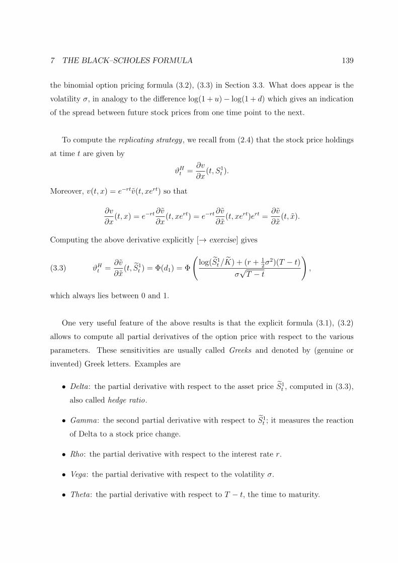
7 THE BLACK–SCHOLES FORMULA 139
the binomial option pricing formula (3.2), (3.3) in Section 3.3. What does appear is the
volatility �, in analogy to the di↵erence log(1 + u)� log(1 + d) which gives an indication
of the spread between future stock prices from one time point to the next.
To compute the replicating strategy , we recall from (2.4) that the stock price holdings
at time t are given by
#H
t=@v
@x(t, S1
t).
Moreover, v(t, x) = e�rt
v(t, xert) so that
@v
@x(t, x) = e
�rt@v
@x(t, xert) = e
�rt@v
@x(t, xert)ert =
@v
@x(t, x).
Computing the above derivative explicitly [! exercise] gives
(3.3) #H
t=@v
@x(t, eS1
t) = �(d1) = �
log(eS1
t/ eK) + (r + 1
2�2)(T � t)
�pT � t
!,
which always lies between 0 and 1.
One very useful feature of the above results is that the explicit formula (3.1), (3.2)
allows to compute all partial derivatives of the option price with respect to the various
parameters. These sensitivities are usually called Greeks and denoted by (genuine or
invented) Greek letters. Examples are
• Delta: the partial derivative with respect to the asset price eS1t, computed in (3.3),
also called hedge ratio.
• Gamma: the second partial derivative with respect to eS1t; it measures the reaction
of Delta to a stock price change.
• Rho: the partial derivative with respect to the interest rate r.
• Vega: the partial derivative with respect to the volatility �.
• Theta: the partial derivative with respect to T � t, the time to maturity.

7 THE BLACK–SCHOLES FORMULA 140
• Vanna: the partial derivative of Delta with respect to �, or the second partial
derivative of the option price, once with respect to eS1tand once with respect to �.
• Vomma: the second partial derivative of the option price with respect to �.
• Charm: the partial derivative of Delta with respect to T � t, the time to maturity.
• Volga: another term for Vomma.
Of course, the above definitions per se make sense for any model; but in the Black–
Scholes model, one has even explicit expressions for them.
Remark. One can find in the literature many di↵erent derivations for the Black–Scholes
formula. One especially popular approach is to first derive the binomial call pricing
formula in the CRR model via arbitrage arguments, as we have done in Section 3.3, and
to then pass to the limit by appropriately rescaling the parameters. More precisely, one
considers for each n 2 IN a binomial model with time step T/n so that letting n increase
corresponds to more and more frequent trading. It is intuitively plausible that the CRR
models should then converge in some sense to the BS model, and one can make this
mathematically precise via Donsker’s theorem. Obtaining the Black–Scholes formula as
a limit is similar but simpler; it is essentially an application of the central limit theorem.
The above limiting “derivation” of the Black–Scholes formula is mathematically much
simpler; but it is also far less satisfactory, especially at the conceptual level. Most impor-
tantly, it does not give the key insight of the methodology behind the formula, namely that
the price is the initial capital for a self-financing replication strategy in the continuous-
time model. We do have the corresponding insight for each binomial model; but the
elementary analysis usually done in the literature does not study whether that important
structural property is preserved when passing to the limit. To obtain that insight (and to
develop it further in other applications or maybe generalisations), stochastic calculus in
continuous time is indispensable.
It is interesting to note that the above view was also shared by the Nobel Prize
Committee; when it awarded the 1997 Nobel Prize in Economics to Robert C. Merton
and Myron Scholes (Fischer Black had died in 1995), the award was given “for a new

7 THE BLACK–SCHOLES FORMULA 141
method to determine the value of derivatives”. The emphasis here is clearly on “method”,
as opposed to “formula”. ⇧

7 THE BLACK–SCHOLES FORMULA 142

8 APPENDIX: SOME BASIC CONCEPTS AND RESULTS 143
8 Appendix: Some basic concepts and results
This short chapter recalls some basic notations, concepts and results from probability
theory. It is not exhaustive and not meant to serve as a replacement for a serious text in
probability theory.
8.1 Very basic things
Let ⌦ 6= ; be a nonempty set. We denote by 2⌦ the power set of ⌦; this is the family of
all subsets of ⌦. A �-field or �-algebra on ⌦ is a family F of subsets of ⌦ which contains
⌦ and which is closed under taking complements and countable unions, i.e. if A 2 F ,
then also Ac2 F , and if Ai, i 2 IN , are in F , then also
Si2IN Ai is in F . Of course, F is
then also closed under countable intersections. A �-field is called finite if it contains only
finitely many sets.
A pair (⌦,F) with ⌦ 6= ; and F a �-algebra on ⌦ is called a measurable space. One
concrete example is (IR,B(IR)), where B(IR) denotes the Borel-�-field on IR. For any
mapping X : ⌦ ! IR and any subset B ✓ IR, we use the shorthand notation
X�1(B) := {X 2 B} := {! 2 ⌦ : X(!) 2 B}.
This is sometimes called the pre-image of the set B under the mapping X. We say that
X is measurable (or more precisely Borel-measurable) if for every B 2 B(IR), we have
{X 2 B} 2 F . One can show that this is equivalent to having {X c} 2 F for every
c 2 IR. More precisely, we could also say that X : ⌦ ! IR is measurable with respect
to F and B(IR). If we replace the measurable space (IR,B(IR)) by another measurable
space (⌦0,F
0), say, we have an analogous definition of a measurable function from ⌦ to
⌦0, with respect to F and F0.
For any subset A of ⌦, the indicator function IA is the function defined by
IA(!) :=
8<
:1 if ! 2 A,
0 if ! 62 A.

8 APPENDIX: SOME BASIC CONCEPTS AND RESULTS 144
The function IA is measurable if and only if A 2 F .
Sometimes, we start with ⌦ 6= ; and a function X : ⌦ ! IR (or more generally to ⌦0).
Then �(X) is by definition the smallest �-field G, say, on ⌦ such thatX is measurable with
respect to G and B(IR) (or G and F0, respectively). We call �(X) the �-field generated
by X. Sometimes, we also consider a �-field generated by a whole family of mappings;
this is then analogously the smallest �-field that makes all the mappings in that family
measurable.
If (⌦,F) is a measurable space, a probability measure on F is a mapping P : F ! [0, 1]
such that P [⌦] = 1 and P is �-additive, i.e.
P
[
i2IN
Ai
�=X
i2IN
P [Ai] whenever Ai, i 2 IN , are sets in F that are pairwise disjoint.
The triple (⌦,F , P ) is then called a probability space.
We say that a statement holds P -almost surely or P -a.s. if the set
A := {! : the statement does not hold}
is a P -nullset, i.e. has P [A] = 0. We sometimes also use instead the formulation that a
statement holds for P -almost all !. For example, X � Y P -a.s. means that P [X < Y ] = 0
or, equivalently, P [X � Y ] = 1. Note that we also use here the shorthand notation
P [X � Y ] := P [{X � Y }] := P [{! 2 ⌦ : X(!) � Y (!)}].
Let (⌦,F , P ) be a probability space and X : ⌦ ! IR a measurable function. We also
say that X is a (real-valued) random variable. If Y is another random variable, we call
X and Y equivalent if X = Y P -a.s. We then denote by L0 or L
0(F) the family of all
equivalence classes of random variables on (⌦,F , P ). For 0 < p < 1, we denote by Lp(P )
the family of all equivalence classes of random variables X which are p-integrable in the
sense that E[|X|p] < 1, and we write then X 2 L
p(P ) or X 2 Lp for short. Finally, L1

8 APPENDIX: SOME BASIC CONCEPTS AND RESULTS 145
is the family of all equivalence classes of random variables that are bounded by a constant
c, say (where the constant can depend on the random variable).
If (⌦,F , P ) is a probability space, then an atom of F is a set A 2 F with the properties
that P [A] > 0 and that if B ✓ A is also in F , then either P [B] = 0 or P [B] = P [A].
Intuitively, atoms are the “smallest P -indivisible sets” in a �-field. Atoms are pairwise
disjoint up to P -nullsets. The space (⌦,F , P ) is called atomless if F contains no atoms;
this can only happen if F is infinite. On the other hand, a finite �-field F can be very
conveniently described via its atoms because every set in F is then a union of atoms.

8 APPENDIX: SOME BASIC CONCEPTS AND RESULTS 146
8.2 Conditional expectations: A survival kit
This section gives a short summary of some basic notions about conditional expectations.
We provide the definition and the most important properties, but hardly any proofs.
Let (⌦,F , P ) be a probability space and U a real-valued random variable, i.e. an
F -measurable mapping U : ⌦ ! IR. Let G ✓ F be a fixed sub-�-field of F ; the intuitive
interpretation is that G gives us some partial information. The goal is then to find a
prediction for U on the basis of the information conveyed by G, or, put di↵erently, a best
estimate for U that uses only information from G.
Definition. A conditional expectation of U given G is a real-valued random variable Y
with the following two properties:
Y is G-measurable.(2.1)
E[UIA] = E[Y IA] for all A 2 G.(2.2)
Y is then called a version of the conditional expectation and is denoted by E[U | G].
Theorem 2.1. Let U be an integrable random variable, i.e. U 2 L1(P ). Then:
1) There exists a conditional expectation E[U | G], and E[U | G] is again integrable.
2) E[U | G] is unique up to P -nullsets: If Y, Y0are random variables satisfying (2.1)
and (2.2), then Y0 = Y P -a.s.
Proof. 1) is nontrivial and not proved here; possible proofs use the Radon–Nikodym
theorem or a projection argument in L2(P ) combined with an extension argument.
2) Due to (2.1), the set A := {Y > Y0} is in G so that (2.2) implies
0 = E[(Y � Y0)IA].
But by the definition of A, we have (Y � Y0)IA � 0 P -a.s., and so we get (Y � Y
0)IA = 0
P -a.s., hence P [A] = 0 by the definition of A, i.e. Y Y0P -a.s. The converse inequality
is proved in the same way. q.e.d.

8 APPENDIX: SOME BASIC CONCEPTS AND RESULTS 147
We next recall without proofs some properties of and computation rules for conditional
expectations. Let U,U 0 be integrable random variables so that E[U | G] and E[U 0| G] exist.
We denote by bG the set of all bounded G-measurable random variables. Then we have:
E[UZ] = E⇥E[U | G]Z
⇤for all Z 2 bG.(2.3)
Linearity: E[aU + bU0| G] = aE[U | G] + bE[U 0
| G] P -a.s., for all a, b 2 IR.
Monotonicity: If U � U0P -a.s., then E[U | G] � E[U 0
| G] P -a.s.
Projectivity : E[U | G] = E⇥E[U | G]
��H⇤
P -a.s., for every �-field H ✓ G.
Further elementary properties are:
E[U | G] = U P -a.s. if U is G-measurable.(2.4)
E⇥E[U | G]
⇤= E[U ].(2.5)
E[ZU | G] = ZE[U | G] P -a.s., for all Z 2 bG.(2.6)
E[U | G] = E[U ] P -a.s. for U independent of G.(2.7)
In fact, (2.4) is clear from the definition, (2.5) follows immediately from (2.2) with A = ⌦,
and (2.6) follows from (2.3) with the help of the definition. The right-hand side of (2.7)
is clearly G-measurable, and U and IA are by assumption independent for every A 2 G;
hence we obtain
E[UIA] = E[U ]E[IA] = E⇥E[U ]IA
⇤
and therefore (2.7), as (2.2) holds as well.
Remarks. 1) Instead of integrability of U , one could also assume that U � 0; then
analogous statements are true. One point of caution applies: if U � 0, then U as well
as E[U | G] could take the value +1, and so one must be careful to avoid expressions
involving 1�1 as these are not well defined.
2) More generally, (2.3) and (2.6) hold as soon as U and ZU are both integrable or
both nonnegative; this is often useful.
3) If U is IRd-valued, one simply does everything component by component to obtain
analogous results. ⇧

8 APPENDIX: SOME BASIC CONCEPTS AND RESULTS 148
For concrete computations of conditional expectations, the following result is often
very useful.
Lemma 2.2. Let U, V be random variables such that U is G-measurable and V is inde-
pendent of G. For every measurable function F � 0 on IR2, we then have
(2.8) E[F (U, V ) | G] = E[F (u, V )]��u=U
=: f(U).
Proof. For F of the form F (u, v) = g(u)h(v) with g, h � 0 and measurable, we have on
the one hand
f(u) = E[F (u, V )] = g(u)E[h(V )]
and on the other hand by (2.6) and (2.7) that
E[F (U, V ) | G] = E[g(U)h(V ) | G] = g(U)E[h(V ) | G] = g(U)E[h(V )] = f(U),
because g(U) is G-measurable and h(V ) is like V independent of G. For general F , one
then uses an argument via the so-called monotone class theorem. q.e.d.
Intuitively, (2.8) says that under the assumptions of Lemma 2.2, one can compute
the conditional expectation E[F (U, V ) | G] by “fixing the known value U and taking the
expectation over the independent quantity V ”.
In analogy to Fatou’s lemma and the dominated convergence theorem, one has the
following convergence results for conditional expectations.
Theorem 2.3. Suppose (Un)n2IN is a sequence of random variables.
1) If Un � X P -a.s. for all n and some integrable random variable X, then
E
hlim infn!1
Un
���Gi lim inf
n!1E[Un | G] P -a.s.
2) If (Un) converges to some random variable U P -a.s. and if |Un| X P -a.s. for all n
and some integrable random variable X, then
(2.9) E
hlimn!1
Un
���Gi= E[U | G] = lim
n!1E[Un | G] P -a.s.
8 APPENDIX: SOME BASIC CONCEPTS AND RESULTS 149
Remark. In analogy to what happens for usual expectations, one might be tempted to
think that (2.9) is still true if one replaces the assumption that all the Un are dominated
by an integrable random variable by the weaker requirement that the sequence (Un) is
uniformly integrable. But while this is still enough to conclude that E[U ] = limn!1 E[Un]
(in fact, one even has convergence of (Un) to U in L1(P )), it does not imply that the
conditional expectations converge P -a.s. (although they then do converge in L1).

8 APPENDIX: SOME BASIC CONCEPTS AND RESULTS 150
8.3 Stochastic processes and functions
Let (⌦,F , P ) be a probability space and T an index set. Usually, we use T = {0, 1, . . . , T}
with some T 2 IN , or T = [0, T ] with some T 2 (0,1), or T = [0,1). A (real-valued)
stochastic process with index set T is then a family of random variables Xt, t 2 T , which
are all defined on the same probability space (⌦,F , P ). We often write X = (Xt)t2T .
Mathematically, a stochastic process can be viewed as a function depending on two
parameters, namely ! 2 ⌦ and t 2 T . If we fix t 2 T , then ! 7! Xt(!) is simply a
random variable. If we fix instead ! 2 ⌦, then t 7! Xt(!) can be viewed as a function
T ! IR, and we often call this the path or the trajectory of the process corresponding
to !. But also viewing a stochastic process as a mapping X : ⌦ ⇥ T ! IR is useful in
some circumstances.
We say that a stochastic process is continuous if all or P -almost all its trajectories
are continuous functions. We call a stochastic process RCLL if all or P -almost all its
trajectories are right-continuous (RC) functions admitting left limits (LL). We say that a
stochastic process is of finite variation if all or P -almost all its trajectories are functions
of finite variation. Recall that a function is of finite variation if and only if it can be
written as the di↵erence of two increasing functions.
Finally, we say that a stochastic process has a property locally if there exists a se-
quence of stopping times (⌧n)n2IN increasing to 1 P -a.s. such that when restricted to the
stochastic interval [[0, ⌧n]] = {(!, t) 2 ⌦⇥ T : 0 t ⌧n(!)}, the process has the prop-
erty under consideration. (Actually, this is a bit tricky. In some cases, for example when
considering integrators, one can simply keep the process constant after ⌧n at its time-⌧n
level; in other cases, for example when considering integrands, one must set the process
to 0 after time ⌧n.)

9 REFERENCES 151
9 References
[1] N. H. Bingham, R. Kiesel: Risk-Neutral Valuation. Pricing and Hedging of Financial
Derivatives, second edition, Springer, 2004
[2] J. Cvitanic, F. Zapatero: Economics and Mathematics of Financial Markets, MIT
Press, 2004
[3] R.-A. Dana, M. Jeanblanc: Financial Markets in Continuous Time, Springer, 2003
[4] F. Delbaen, W. Schachermayer: The Mathematics of Arbitrage, Springer, 2006
[5] C. Dellacherie, P.-A. Meyer: Probabilities and Potential B. Theory of Martingales,
North-Holland, 1982
[6] R. Durrett: Probability. Theory and Examples, fourth edition, Cambridge University
Press, 2010
[7] R. J. Elliott, P. E. Kopp:Mathematics of Financial Markets, second edition, Springer,
2005
[8] H. Follmer: Calcul d’Ito sans probabilites, Seminaire de Probabilites XV, Lecture
Notes in Mathematics 850, Springer, 1981, pp. 143–150
[9] H. Follmer, A. Schied: Stochastic Finance. An Introduction in Discrete Time, third
edition, de Gruyter, 2011
[10] J. Jacod, P. Protter: Probability Essentials, second edition, Springer, 2003
[11] J. Jacod, A. N. Shiryaev: Limit Theorems for Stochastic Processes, second edition,
Springer, 2003
[12] D. Lamberton, B. Lapeyre: Introduction to Stochastic Calculus Applied to Finance,
second edition, Chapman & Hall/CRC, 2008
[13] P. E. Protter: Stochastic Integration and Di↵erential Equations, second edition, ver-
sion 2.1, Springer, 2005

152

10 INDEX 153
10 Index
L2loc(M), 94
P -augmented filtration, 124
X-integrable, 104
F⌧ , 77
M20, loc, 94
a-admissible, 20
(NFLVR), 43
(predictable) compensator, 88
(NA), 31
adapted, 5
admissible, 20
American option, 52
arbitrage opportunity, 31
arbitrage-free, 31
arc length, 73
atom, 27
attainable, 54
bank account, 9
barrier option, 81
Bayes formula, 46, 117
Bichteler–Dellacherie theorem, 103
binomial call pricing formula, 65
binomial model, 7, 62
Black–Scholes formula, 138
Black–Scholes model, 127
boundary condition, 136
bounded elementary process, 89
branch, 27
Brownian motion (with respect to filtra-
tion), 69
Brownian motion with (instantaneous) drift,
120
canonical decomposition, 101
canonical model, 26
change of numeraire, 64
complete, 59
contingent claim, 51
cost process, 13
covariation process, 87
Cox–Ross–Rubinstein model, 7, 62
credit risk, 133
density, 45
density process, 45, 117
discounting, 9, 62, 65, 128, 137, 138
dominated convergence theorem, 103
doubling strategy, 18
drift, 128
dual martingale measure, 64
dynamic portfolio, 11
equivalent martingale measure, 39
equivalent martingale measure, construc-
tion, 47
equivalent probability measures, 34
European call option, 52, 62, 138
European option, 51

10 INDEX 154
events observable up to time �, 77
filtration, 5, 69
filtration, generated by a process, 6
finite variation, 73
frictionless financial market, 10
FTAP, 43
fundamental theorem of asset pricing, 43,
60
gains process, 13
geometric Brownian motion, 112
Girsanov’s theorem, 103, 118, 119
Greeks, 139
hitting time, 79
i.i.d. returns, 7
incomplete, 59
increment (of a process), 13
interest rate, 127
isometry property, 89
Ito process, 114
Ito’s formula, 103, 107, 110
Ito’s representation theorem, 124
Laplace transform, 81
law of large numbers, 71
law of the iterated logarithm, 71
local martingale, 22
local martingale null at 0, 78
localisation, 94
localised class, 94
localising sequence, 22, 78
locally bounded, 95
locally equivalent probability measures,
117
market price of risk, 129
Markov property, 82
martingale, 21, 76
martingale approach, 134
martingale property, 21
mesh size, 73
multinomial model, 7
no free lunch with vanishing risk, 43
node, 27
Novikov condition, 121
numeraire, 9
one-step transition probabilities, 27
optional decomposition theorem, 56
optional quadratic variation, 87
partial di↵erential equation, 135
partition, 73
path space, 26
payo↵, 51
payo↵ stream, 52
PDE approach, 134
portfolio, 11
predictable, 5, 91
predictable �-field, 91
predictable (process), 91
product rule, 115

10 INDEX 155
quadratic variation, 72, 74, 106
Radon–Nikodym, 45
RCLL, 76
recombining tree, 28
reference asset, 9
replicating strategy, 54, 132, 139
risk-neutral measure, 57
risk-neutral valuation, 57
risky assets, 9
ruin problem for Brownian motion, 115
Samuelson model, 127
second fundamental theorem of asset pric-
ing, 60
self-financing, 14, 132
semimartingale, 101
separating hyperplane, 41
sharp bracket, 88
Sharpe ratio, 129
special, 101
square bracket, 87
stochastic di↵erential equation, 112
stochastic exponential, 113
stochastic integral, 14, 85, 89
stochastic interval, 94
stochastic logarithm, 119
stochastic volatility, 133
stopped process, 17
stopping theorem, 77
stopping time, 17, 76
strong Markov property, 82
submartingale, 21, 76
supermartingale, 21, 76
trading dates, 5
trading strategy, 11, 131
transformations of Brownian motion, 70
tree, 27
tree, non-recombining, 27, 65
tree, recombining, 28, 67
trivial �-field, 9
usual conditions, 69
value process, 11
vector stochastic integral, 95
volatility, 128