Lecture Notes on

CAD-CIM

III B. Tech VI semester

Prepared by

Dr. D GOVARDHAN,

Professor & Head, AE

DEPARTMENT OF AERONAUTICAL ENGINEERING

INSTITUTE OF AERONAUTICAL ENGINEERING (Autonomous)

Dundigal, Hyderabad, Telangana 500043

SYLLABUS

UNIT-I INTRODUCTION

Computers in industrial manufacturing , product cycle, CAD/CAM hardware, basic structure, CPU,

memory types, input devices, display devices, hard copy devices, and storage devices, computer

graphics, raster scan graphics coordinate system, database structure for graphics modeling,

transformation of geometry, three dimensional transformations, mathematics of projections,

clipping, hidden surface removal.

UNIT-II GEOMETRICAL MODELLING

Requirements, geometric models, geometric construction models, curve representation methods,

surface representation methods, modeling facilities desired, drafting and modeling systems, basic

geometric commands, layers, display control commands, editing, dimensioning and solid

modeling.

UNIT-III GROUP TECHNOLGY COMPUTER AIDED PROCESS PLANNING

History of group technology, role of G.T in CAD/CAM integration, part families, classification and

coding, DCLASS and MCLASS and OPTIZ coding systems, facility design using G.T, benefits of

G.T, cellular manufacturing. Process planning, role of process planning in CAD/CAM integration,

approaches to computer aided process planning, variant approach and generative approaches,

CAPP and CMPP systems.

UNIT-IV COMPUTER AIDED PLANNING AND CONTROL, SHOP FLOOR CONTROL

AND INTRODUCTION TO FMS

Production planning and control, cost planning and control, inventory management, material

requirements planning (ERP), control, phases, factory data collection system, automatic

identification methods, bar code technology, automated data collection system; FMS, components

of FMS, types, FMS workstation, material handling and storage system, FMS layout, computer

control systems, applications and benefits.

UNIT-V COMPUTER AIDED PLANNING AND CONTROL AND COMPUTER

MONITORING

Production planning and control, cost planning and control, inventory management, material

requirements planning (MRP), shop floor control, lean and agile manufacturing, types of

production monitoring systems, structure model of manufacturing, process control and strategies,

direct digital control.

Text Books:

1. A. Zimmers, P. Groover, ―CAD/ CAM‖, Prentice- Hall India, 2008. 2. Zeid, Ibrahim, ―CAD / CAM Theory and Practice‖, Tata McGraw-Hill, 1997. 3. Mikell. P.Groover ―Automation, Production Systems and Computer Integrated

Manufacturing‖, Pearson Education 2001. 4. Ranky, Paul G., ―Computer Integrated Manufacturing‖, Prentice hall of India Pvt. Ltd.,2005 5. Yorem Koren, ―Computer Integrated Manufacturing‖, McGraw Hill, 2005.

Reference Books:

1. P. Groover, Automation, ―Production Systems & Computer Integrated Manufacturing‖,

Pearson Education.2nd Edition 1989.

2. Lalit Narayan, ―Computer Aided Design and Manufacturing‖, Prentice-Hall India.3rd

Edition 2002.

3. Radhakrishnan, Subramanian, ―CAD / CAM / CIM‖, New Age.4th Edition 2016. 4. Jami J Shah, Martti Mantyla, ―Parametric and Feature-Based CAD/CAM: Concepts,

Techniques, and Applications‖, John Wiley & Sons Inc, 1995.

5. Alavala, ―CAD/ CAM: Concepts and Applications‖, PHI Publications, 4th Edition, 2016.

6. W. S. Seames,- Computer Numerical Control Concepts and Programming‖, 4th Edition

1999.

3

UNIT 1

INTRODUCTION

CAD/CAM

CAD/CAM is a term which means computer-aided design and computer- aided

manufacturing. It is the technology concerned with the use of digital computers to perform certain

functions in design and production. This technology is moving in the direction of greater

integration of design and manufacturing, two activities which have traditionally been treated as

distinct and separate functions in a production firm. Ultimately, CAD/CAM will provide the

technology base for the computer-integrated factory of the future.

Computer-aided design (CAD) can be defined as the use of computer systems to

assist in the creation, modification, analysis, or optimization of a design. The computer

systems consist of the hardware and software to perform the specialized design functions

required by the particular user firm. The CAD hardware typically includes the computer, one or

more graphics display terminals, keyboards, and other peripheral equipment. The CAD

software consists of the computer programs to implement computer graphics on the system

plus application programs to facilitate the engineering functions of the user company. Examples

of these application programs include stress-strain analysis of components, dynamic response of

mechanisms, heat-transfer calculations, and numerical control part programming. The collection

of application programs will vary from one user firm to the next because their product lines,

manufacturing processes, and customer markets are different. These factors give rise to differences

in CAD system requirements.

Computer-aided manufacturing (CAM) can be defined as the use of computer

systems to plan, manage, and control the operations of a manufacturing plant through either

direct or indirect computer interface with the plant's production resources. As indicated by the

definition, the applications of computer-aided manufacturing fall into two broad categories:

1. Computer monitoring and control. These are the direct applications in which

the computer is connected directly to the manufacturing process for the purpose of

monitoring or controlling the process.

2. Manufacturing support applications. These are the indirect applications in which

the computer is used in support of the production operations in the plant, but there

is no direct interface between the computer and the manufacturing process.

4

The distinction between the two categories is fundamental to an understanding

of computer-aided manufacturing. It seems appropriate to elaborate on our brief definitions of the

two types.

Computer monitoring and control can be separated into monitoring applications

and control applications. Computer process monitoring involves a direct computer interface with

the manufacturing process for the purpose of observing the process and associated equipment

and collecting data from the process. The computer is not used to control the operation

directly. The control of the process remains in the hands of human operators, who may be

guided by the information compiled by the computer.

Computer process control goes one step further than monitoring by not only observing

the process but also controlling it based on the observations. The distinction between

monitoring and control is displayed in Figure. With computer monitoring the flow of data

between the process and the computer is in one direction only, from the process to the computer.

In control, the computer interface allows for a two-way flow of data. Signals are transmitted

from the process to the computer, just as in the case of computer monitoring. In addition, the

computer issues command signals directly to the manufacturing process based on control

algorithms contained in its software.

In addition to the applications involving a direct computer-process interface for the purpose of

process monitoring and control, computer-aided manufacturing also includes indirect

applications in which the computer serves a support role in the manufacturing operations of

the plant. In these applications, the computer is not linked directly to the manufacturing

process.

(a) computer monitoring, (b) computer control.

Instead, the computer is used "off-line" to provide plans, schedules, forecasts, instructions,

and information by which the firm's production resources can be managed more effectively.

The form of the relationship between the computer and the process is represented symbolically

5

in Figure. Dashed lines are used to indicate that the communication and control link is an off-

line connection, with human beings often required to consumate the interface. Some

examples of CAM for manufacturing support that are discussed in subsequent chapters of

this book include:

Numerical control part programming by computers. Control programs are prepared for

automated machine tools.

Computer-automated process planning. The computer prepares a listing of the operation

sequence required to process a particular product or component.

Computer-generate work standards. The computer determines the time standard for a

particular production operation.

Production scheduling. The computer determines an appropriate schedule for meeting

production requirements.

Material requirements planning. The computer is used to determine when to order raw

materials and purchased components and how many should be ordered to achieve the

production schedule.

Shop floor control. In this CAM application, data are collected from the factory to

determine progress of the various production shop orders.

In all of these examples, human beings are presently required in the application either to

provide input to the computer programs or to interpret the computer output and implement the

required action.

CAM for manufacturing support.

6

THE PRODUCT CYCLE AND CAD/CAM

For the reader to appreciate the scope of CAD/CAM in the operations of a manufacturing

firm, it is appropriate to examine the various activities and functions that must be accomplished

in the design and manufacture of a product. We will refer to these activities and functions as the

product cycle.

A diagram showing the various steps in the product cycle is presented in Figure 1.1. The

cycle is driven by customers and markets which demand the product. It is realistic to think of

these as a large collection of diverse industrial and consumer markets rather than one monolithic

market. Depending on the particular customer group, there will be differences in the way the

product cycle is activated. In some cases, the design functions are performed by the customer and

the product is manufactured by a different firm. In other cases, design and manufacturing is

accomplished by the same firm. Whatever the case, the product cycle begins with a concept, an

idea for a product. This concept is cultivated, refined, analyzed, improved, and translated into

a plan for the product through the design engineering process. The plan is documented by drafting

Ii set of engineering drawings showing how the product is made and providing a set of

specifications indicating how the product should perform.

PRODUCT CYCLE IN CONVENTIONAL ENVIRONMENT

7

Except for engineering changes which typically follow the product throughout its life

cycle, this completes the design activities in Figure. The next activities involve the

manufacture of the product. A process plan is formulated which

specifies the sequence of production operations required to make the product. New equipment and

tools must sometimes be acquired to produce the new product. Scheduling provides a plan

that commits the company to the manufacture of certain quantities of the product by certain dates.

Once all of these plans are formulated, the product goes into production, followed by quality

testing, and delivery to the customer.

Product cycle (design and manufacturing).

The impact of CAD/CAM is manifest in all of the different activities in the product cycle, as

indicated in Figure. Computer-aided design and automated drafting are utilized in the

conceptualization, design, and documentation of the product. Computers are used in process

planning and scheduling to perform these functions more efficiently. Computers are used in

production to monitor and control the manufacturing operations. In quality control,

computers are used to perform inspections and performance tests on the product and its

components.

Fig 1.2: Product cycle in an computerised environment

8

As illustrated in Figure 1.2, CAD/CAM is overlaid on virtually all of the activities and

functions of the product cycle. In the design and production operations of a modem

manufacturing firm, the computer has become a pervasive, useful, and indispensable tool. It is

strategically important and competitively imperative that manufacturing firms and the

people who are employed by them understand CAD/CAM.

AUTOMATION AND CAD/CAM Automation is defined as the technology concerned with the application of complex

mechanical, electronic, and computer-based systems in the operation and control of

production. It is the purpose of this section to establish the relationship between CAD/CAM

and automation.

As indicated in previous Section, there are differences in the way the product cycle is

implemented for different firms involved in production. Production activity can be divided into

four main categories:

l. Continuous-flow processes

2. Mass production of discrete products

3. Batch production

4. Job shop production

The definitions of the four types are given in Table. The relationships among the four

types in terms of product variety and production quantities can be conceptualized as shown in

Figure. There is some overlapping of the categories as the figure indicates. Table provides

a list of some of the notable achievements in automation technology for each of the four

production types.

One fact that stands out from Table is the importance of computer technology in

automation. Most of the automated production systems implemented today make use of

computers. This connection between the digital computer and manufacturing automation may

seem perfectly logical to the reader. However, this logical connection has not always existed.

For one thing, automation technology

9

1.1: TABLE Four Types of Production

Category Description

l. Continuous-flow

processes

Continuous dedicated production of large amounts of bulk

product. Examples include continuous chemical plants and

oil refineries

2. Mass production of

discrete products

Dedicated production of large quantities of one product (with

perhaps limited model variations). Examples include

automobiles, appliances, and engine blocks.

3. Batch production Production of medium lot sizes of the same product or

component. The lots may be produced once or repeated periodically. Examples include books, clothing, and certain

industrial machinery.

4. Job shop production Production of low quantities, often one of a kind, of specialized

products. The products are often customized and technologically complex. Examples include prototypes, aircraft, machine tools,

and other equipment

Fig: 1.3 Four production types related to quantity and product variation

10

TABLE Automation Achievements for the Four Types of Production

Category

Automation achievements

l. Continuous-flow processes

Flow process from beginning to end

Sensor technology available to measure important process variables

Use of sophisticated control and optimization strategies

Fully computer-automated plants

2. Mass production

of discrete products

Automated transfer machines

Dial indexing machines

Partially and fully automated assembly lines

Industrial robots for spot welding, parts handling, machine loading,

spray painting, etc.

Automated materials handling systems

Computer production monitoring

3. Batch production Numerical control (NC), direct numerical control (DNC), computer

numerical control (CNC)

Adaptive control machining

Robots for arc welding, parts handling, etc. Computer-

integrated manufacturing systems

4. Job shop

production

Numerical control, computer numerical control

FUNDAMENTALS OF CAD

INTRODUCTION The computer has grown to become essential in the operations of business, government, the

military, engineering, and research. It has also demonstrated itself, especially in recent years, to

be a very powerful tool in design and manufacturing. In this and the following two chapters,

we consider the application of computer technology to the design of a product. This

secton provides an overview of computer-aided design.

The CAD system defined

As defined in previous section, computer-aided design involves any type of design activity

which makes use of the computer to develop, analyze, or modify an engineering design. Modem

CAD systems (also often called CAD/CAM systems) are based on interactive computer

11

graphics (ICG).Interactive computer graphics denotes a user-oriented system in which the

computer is employed to create, transform, and display data in the form of pictures or symbols.

The user in the computer graphics design system is the designer, who communicates data

and commands to the computer through any of several input devices. The computer

communicates with the user via a cathode ray tube (CRT). The designer creates an image on

the CRT screen by entering commands to call the desired software sub-routines stored in

the computer. In most systems, the image is constructed out of basic geometric elements- points,

lines, circles, and so on. It can be modified according to the commands of the designer-

enlarged, reduced in size, moved to another location on the screen, rotated, and other

transformations. Through these various manipulations, the required details of the image are

formulated.

The typical ICG system is a combination of hardware and software. The hardware includes

a central processing unit, one or more workstations (including the graphics display terminals),

and peripheral devices such as printers. Plotters, and drafting equipment. Some of this

hardware is shown in Figure. The software consists of the computer programs needed to

implement graphics processing on the system. The software would also typically include

additional specialized application programs to accomplish the particular engineering

functions required by the user company.

It is important to note the fact that the ICG system is one component of a computer-aided design

system. As illustrated in Figure, the other major component is the human designer. Interactive

computer graphics is a tool used by the designer to solve a design problem. In effect, the

ICG system magnifies the powers of the designer. This bas been referred to as the

synergistic effect. The designer performs the portion of the design process that is most

suitable to human intellectual skills (conceptualization, independent thinking); the computer

performs the task: best suited to its capabilities (speed of calculations, visual display,

storage of large data), and the resulting system exceeds the sum of its components.

There are several fundamental reasons for implementing a computer-aided design system.

l. To increase the productivity of the designer. This is accomplished by helping the

designer to the product and its component subassemblies and parts; and by reducing

the time required in synthesizing, analyzing, and documenting the design. This

productivity improvement translates not only into lower design cost but also into shorter

project completion times.

12

2. To improve the quality of design. A CAD system permits a more thorough

engineering analysis and a larger number of design alternatives can be investigated.

Design errors are also reduced through the greater accuracy provided by the system.

These factors lead to a better design.

3. To improve communications. Use of a CAD system provides better engineering

drawings, more standardization in the drawings, better documentation of the design, fewer

drawing errors and greater legibility.

4. To create a database for manufacturing. In the process of creating the documentation

for the product design (geometries and dimensions of the product and its components,

material specifications for components, bill of materials, etc.), much of the required

database to manufacture the product is also created.

THE DESIGN PROCESS Before examining the several facets of computer-aided design, let us first consider the

general design process. The process of designing something is characterized by

Shigley as an iterative procedure, which consists of six identifiable steps or phases:-

l. Recognition of need

2. Definition of problem

3. Synthesis

4. Analysis and optimization

5. Evaluation

6. Presentation

Recognition of need involves the realization by someone that a problem exists for which

some corrective action should be taken. This might be the identification of some defect

in a current machine design by an engineer or the perception of a new product marketing

opportunity by a salesperson. Definition of the problem involves a thorough specification of

the item to be designed. This specification includes physical and functional characteristics,

cost, quality, and operating performance.

Synthesis and analysis are closely related and highly interactive in the design process. A

certain component or subsystem of the overall system is conceptualized by the designer,

subjected to analysis, improved through this analysis procedure, and redesigned. The process

13

is repeated until the design has been optimized within the constraints imposed on the

designer. The components and subsystems are synthesized into the final overall system in a

similar interactive manner.

Evaluation is concerned with measuring the design against the specifications established in

the problem definition phase. This evaluation often requires the fabrication and testing of

a prototype model to assess operating performance, quality, reliability, and other criteria. The

final phase in the design process is the presentation of the design. This includes

documentation of the design by means of drawings, material specifications, assembly lists,

and so on. Essentially, the documentation requires that a design database be created. Figure

illustrates the basic steps in the design process, indicating its iterative nature.

Fig 1.4: The general design process as defined by Shigley .

14

Engineering design has traditionally been accomplished on drawing boards, with the design

being documented in the form of a detailed engineering drawing. Mechanical design includes

the drawing of the complete product as well as its components and subassemblies, and the

tools and fixtures required to manufacture the product. Electrical design is concerned

with the preparation of circuit diagrams, specification of electronic components, and so on.

Similar manual documentation is required in other engineering design fields (structural

design, aircraft design, chemical engineering design, etc.). In each engineering

discipline, the approach has traditionally been to synthesize a preliminary design

manually and then to subject that design to some form of analysis. The analysis may involve

sophisticated engineering calculations or it may involve a very subjective judgment of the

aesthete appeal possessed by the design. The analysis procedure identifies certain

improvements that can he made in the design. As stated previously, the process is

iterative. Each iteration yields an improvement in the design. The trouble with this iterative

process is that it is time consuming. Many engineering labor hours are required to

complete the design project.

THE APPLICATION OF COMPUTERS FOR DESIGN The various design-related tasks which are performed by a modem computer-aided design-system

can be grouped into four functional areas:

l. Geometric modeling

2. Engineering analysis

3. Design review and evaluation

4. Automated drafting

These four areas correspond to the final four phases in Shigley's general design process,

illustrated in Figure. Geometric modeling corresponds to the synthesis phase in which

the physical design project takes form on the ICG system. Engineering analysis corresponds to

phase 4, dealing with analysis and optimization. Design review and evaluation is the fifth step

in the general design procedure. Automated drafting involves a procedure for converting

the design image data residing in computer memory into a hard-copy document. It

represents an important method for presentation (phase 6) of the design. The following four

sections explore each of these four CAD functions.

15

Geometric modeling

In computer-aided design, geometric modeling is concerned with the computer-

compatible mathematical description of the geometry of an object. The mathematical

description allows the image of the object to be displayed and manipulated on a

graphics terminal through signals from the CPU of the CAD system. The software that

provides geometric modeling capabilities must be designed for efficient use both by the

computer and the human designer.

To use geometric modeling, the designer constructs, the graphical image of the object on

the CRT screen of the ICG system by inputting three types of commands to the

computer. The first type of command generates basic geometric elements such as points,

lines, and circles. The second command type is used to accomplish scaling, rotating, or

other transformations of these elements. The third type of command causes the various

elements to be joined into the desired shape of the object being creaed on the ICG system.

During the geometric modeling process, the computer converts the commands into a

16

mathematical model, stores it in the computer data files, and displays it as an image on the

CRT screen. The model can subsequently be called from the data files for review, analysis, or

alteration.

There are several different methods of representing the object in geometric modeling. The

basic form uses wire frames to represent the object. In this form, the object is displayed by

interconnecting lines as shown in Figure. Wire frame geometric modeling is classified

into three types depending on the capabilities of the ICG system.

The three types are:

l. 2D. Two-dimensional representation is used for a flat object.

2. 2½D. This goes somewhat beyond the 2D capability by permitting a three-

dimensional object to be represented as long as it has no side-wall details.

3. 3D. This allows for full three-dimensional modeling of a more complex geometry.

Example of wire-frame drawing of a part.

Even three-dimensional wire-frame representations of an object are sometimes inadequate for

complicated shapes. Wire-frame models can be enhanced by several different methods.

Figure shows the same object shown in the previous figure but with two possible

improvements. lbe first uses dashed lines to portray the rear edges of the object, those

which would be invisible from the front. lbe second enhancement removes the

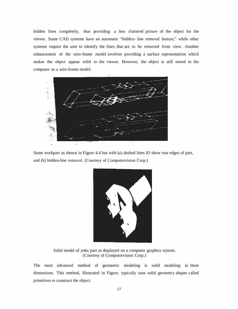
17

hidden lines completely, thus providing a less cluttered picture of the object for the

viewer. Some CAD systems have an automatic "hidden- line removal feature," while other

systems require the user to identify the lines that are to be removed from view. Another

enhancement of the wire-frame model involves providing a surface representation which

makes the object appear solid to the viewer. However, the object is still stored in the

computer as a wire-frame model.

Same workpart as shown in Figure 4.4 but with (a) dashed lines lO show rear edges of part,

and (b) hidden-line removal. (Courtesy of Computervision Corp.)

Solid model of yoke part as displayed on a computer graphics system.

(Courtesy of Computervision Corp.)

The most advanced method of geometric modeling is solid modeling in three

dimensions. This method, illustrated in Figure, typically uses solid geometry shapes called

primitives to construct the object.

18

Another feature of some CAD systems is color graphics capability. By means of colour,

it is possible to display more information on the graphics screen. Colored images help to

clarify components in an assembly, or highlight dimensions, or a host of other purposes.

Engineering analysis

In the formulation of nearly any engineering design project, some type of analysis is required.

The analysis may involve stress-strain calculations, heat-transfer computations, or the use of

differential equations to describe the dynamic behavior of the system being designed. The

computer can be used to aid in this analysis work. It is often necessary that specific

programs be developed internally by the engineering analysis group to solve a particular

design problem. In other situations, commercially available general-purpose programs can be

used to perform the engineering analysis.

Turnkey CAD/CAM systems often include or can be interfaced to engineering

analysis software which can be called to operate on the current design model.

Two important examples of this type:

1. Analysis of mass properties

2. Finite-element analysis

The analysis of mass properties is the analysis feature of a CAD system that has probably

the widest application. It provides properties of a solid object being analyzed, such as the

surface area, weight, volume, center of gravity, and moment of inertia. For a plane surface (or

a cross section of a solid object) the corresponding computations include the perimeter, area,

and inertia properties.

Probably the most powerful analysis feature of a CAD system is the finite-

element method. With this technique, the object is divided into a large number of

finite elements (usually rectangular or triangular shapes) which form an

interconnecting network of concentrated nodes. By using a computer with significant

computational capabilities, the entire Object can be analyzed for stress-strain, heat

transfer, and other characteristics by calculating the behavior of each node. By

determining the interrelating behaviors of all the nodes in the system, the behavior of

the entire object can be assessed.

Some CAD systems have the capability to define automatically the nodes

and the network structure for the given object. lbe user simply defines certain

19

parameters for the finite-element model, and the CAD system proceeds with the

computations.

The output of the finite-element analysis is often best presented by the

system in graphical format on the CRT screen for easy visualization by the user, For

example, in stress-strain analysis of an object, the output may be shown in the form

of a deflected shape superimposed over the unstressed object. This is illustrated in

Figure. Color graphics can also be used to accentuate the comparison before and

after deflection of the object. This is illustrated in Figure for the same image as that

shown in Figure . If the finite-element analysis indicates behavior of the design

which is undesirable, the designer can modify the shape and recompute the finite-

element analysis for the revised design.

Finite-element modeling for stress-strain analysis. Graphics display shows strained

part superimposed on unstrained part for comparison.

Design review and evaluation

Checking the accuracy of the design can be accomplished conveniently on

the graphics terminal. Semiautomatic dimensioning and tolerancing routines which

assign size specifications to surfaces indicated by the user help to reduce the

possibility of dimensioning errors. The designer can zoom in on part design details

and magnify the image on the graphics screen for close scrutiny.

A procedure called layering is often helpful in design review. For example,

a good application of layering involves overlaying the geometric image of the final

shape of the machined part on top of the image of the rough casting. This ensures

20

that sufficient material is available on the casting to acccomplish the final machined

dimensions. This procedure can be performed in stages to check each successive step

in the processing of the part.

Another related procedure for design review is interference checking. This

involves the analysis of an assembled structure in which there is a risk that the

components of the assembly may occupy the same space. This risk occurs in the

design of large chemical plants, air-separation cold boxes, and other complicated

piping structures.

One of the most interesting evaluation features available on some computer-

aided design systems is kinematics. The available kinematics packages provide the

capability to animate the motion of simple designed mechanisms such as hinged

components and linkages. This capability enhances the designer‘s visualization of the

operation of the mechanism and helps to ensure against interference with other

components. Without graphical kinematics on a CAD system, designers must often

resort to the use of pin-and-cardboard models to represent the mechanism.

commercial software packages are available to perform kinematic analysis. Among

these are programs such as ADAMS (Automatic Dynamic Analysis of Mechanical

Systems), developed at the University of Michigan. This type of program can be very

useful to the designer in constructing the required mechanism to accomplish a

specified motion and/or force.

Automated drafting

Automated drafting involves the creation of hard-copy engineering

drawings directly from the CAD data base. In some early computer-aided design

departments, automation of the drafting process represented the principal

justification for investing in the CAD system. Indeed, CAD systems can increase

productivity in the drafting function by roughly five times over manual drafting.

Some of the graphics features of computer-aided design systems lend them-

selves especially well to the drafting process. These features include automatic

dimensioning, generation of crosshatched areas, scaling of the drawing, and the

capability to develop sectional views and enlarged views of particular path details.

The ability to rotate the part or to perform other transformations of the image (e.g.,

oblique, isometric, or perspective views), as illustrated in Figure, can be of

significant assistance in drafting. Most CAD systems are capable of generating as

21

many as six views of the part. Engineering drawings can be made to adhere to

company drafting standards by programming the standards into the CAD system.

Figure shows an engineering drawing with four views displayed. This drawing was

produced automatically by a CAD system. Note how much the isometric view

promotes a higher level of understanding of the object for the user than the three

orthographic views.

Parts classification and coding

In addition to the four CAD functions described above, another feature of

the CAD data base is that it can be used to develop a parts classification and coding

system. Parts classification and coding involves the grouping of similar part designs

into classes, and relating the similarities by mean of a coding scheme. Designers can

use the classification and coding system to retrieve existing part designs rather than

always redesigning new parts.

CREATING THE MANUFACTURING DATA BASE

Another important reason for using a CAD system is that it offers the

opportunity to develop the data base needed to manufacture the product. In the

conventional manufacturing cycle practiced for so many years in industry,

engineering drawings were prepared by design draftsmen and then used by

manufacturing engineers to develop the process plan (i.e., the "route sheets"). The

activities involved in designing the product were separated from the activities

associated with process planning. Essentially, a two-step procedure was employed.

This was both time consuming and involved duplication of effort by design and

manufacturing personnel. In an integrated CAD/CAM system, a direct link is

established between product design and manufacturing: It" is the goal of CAD/CAM

not only to automate certain phases of design and certain phases of manufacturing,

but also to automate the transition from design to manufacturing. Computer-based

systems have been developed which create much of the data and documentation

required to plan and manage the manufacturing operations for the product.

The manufacturing data base is an integrated CAD/CAM data base. It

includes all the data on the product generated during design (geometry data, bill of

materials and parts lists, material specifications, etc.) as well as additional data

required for manufacturing much of which is based Oll the product design. Figure

22

4.lO shows how the CAD/CAM data base is related to design and manufacturing in a

typical production-oriented company.

FIGURE Desirable relationship of CAD/CAM data base to CAD and CAM.

BENERTS OF COMPUTER-AIDED DESIGN

There are many benefits of computer-aided design, only some of which can

be easily measured. Some of the benefits are intangible, reflected in improved work

quality, more pertinent and usable information, and improved control, all of which

are difficult to quantify. Other benefits are tangible, but the savings from them show

up far downstream in the production process, so that it is difficult to assign a dollar

figure to them in the design phase. Some of the benefits that derive from

implementing CAD/CAM can be directly measured. Table provides a checklist of

potential benefits of an integrated CAD/CAM system. In the subsections that follow,

we elaborate on some of these advantages.

Productivity improvement in design

Increased productivity translates into a more competitive position for the

firm because it will reduce staff requirements on a given project. This leads to lower

costs in addition to improving response time on projects with tight schedules.

Surveying some of the larger CAD/CAM vendors, one finds that the

Productivity improvement ratio for a designer/draftsman is usually given as a range,

typically from a low end of 3: l to a high end in excess of lO: l (often far in excess

of that figure). There are individual cases in which productivity has been increased

by a factor of lOO, but it would be inaccurate to represent that figure as typical.

TABLE Potential Benefits That May Result from implementing CAD as

Part of an Integrated CAD/CAM System.

23

l. Improved engineering productivity

2. Shorter lead times

3. Reduced engineering personnel requirements

4. Customer modifications are easier to make

5. Faster response to requests for quotations

6. Avoidance of subcontracting to meet schedules

7. Minimized transcription errors

8. Improved accuracy of design

9. In analysis, easier recognition of component interactions

lO. Provides better functional analysis to reduce prototype testing

ll. Assistance in preparation of documentation

l2. Designs have more standardization

l3. Better designs provided

l4. Improved productivity in tool design

l5. Better knowledge of costs provided

l6. Reduced training time for routine drafting tasks and NC part

programming

l7. Fewer errors in NC part programming

l8. Provides the potential for using more existing parts and tooling

l9. Helps ensure designs are appropriate to existing manufacturing

techniques

20. Saves materials and machining time by optimization algorithms

21. Provides operational results on the status of work in progress

22. Makes the management of design personnel on projects more effective

23. Assistance in inspection of complicated parts

24. Better communication interfaces and greater understanding among

engineers, designers, drafters, management, and different project

groups.

Productivity improvement in computer-aided design as compared to the

traditional design process is dependent on such factors as:

Complexity of the engineering drawing

Level of detail required in the drawing

Degree of repetitiveness in the designed parts

Degree of symmetry in the parts

Extensiveness of library of commonly used entities

As each of these factors is increased. the productivity advantage of CAD

24

will tend to increase

Shorter lead times

Interactive computer-aided design is inherently faster than the traditional

design. It also speeds up the task of preparing reports and lists (e.g., the assembly

lists) which are normally accomplished manually. Accordingly, it is possible with a

CAD system to produce a finished set of component drawings and the associated

reports in a relatively short time. Shorter lead times in design translate into shorter

elapsed time between receipt of a customer order and delivery of the final product.

The enhanced productivity of designers working with CAD systems will tend to

reduce the prominence of design, engineering analysis, and drafting as critical time

elements in the overall manufacturing lead time.

Design analysis

The design analysis routines available in a CAD system help to consolidate

the design process into a more logical work pattern. Rather than having a back- and-

forth exchange between design and analysis groups, the same person can perform the

analysis while remaining at a CAD workstation. This helps to improve the

concentration of designers, since they are interacting with their designs in a real-time

sense. Because of this analysis capability, designs can be created which are closer to

optimum. There is a time saving to be derived from the computerized analysis

routines, both in designer time and in elapsed time. This saving results from the rapid

response of the design analysis and from the tune no longer lost while the design

finds its way from the designer's drawing board to the design analyst's queue and

back again.

Fewer design errors

Interactive CAD systems provide an intrinsic capability for avoiding design,

drafting, and documentation errors. Data entry, transposition, and extension errors

that occur quite naturally during manual data compilation for preparation of a bill of

materials are virtually eliminated. One key reason for such accuracy is simply that

No manual handling of information is required once the initial drawing has

been developed. Errors are further avoided because interactive CAD systems perform

time-consuming repetitive duties such as multiple symbol placement, and sorts by

area and by like item, at high speeds with consistent and accurate results. Still more

errors can be avoided because a CAD system, with its interactive capabilities, can be

25

programmed to question input that may be erroneous. For example, the system might

question a tolerance of O.OOOO2 in. It is likely that the user specified too many zeros.

The success of this checking would depend on the ability of the CAD system

designers to determine what input is likely to be incorrect and hence, what to

question.

Greater accuracy in design calculations

There is also a high level of dimensional control, far beyond the levels of

accuracy attainable manually. Mathematical accuracy is often to l4 significant

decimal places. The accuracy delivered by interactive CAD systems in three-

dimensional curved space designs is so far behind that provided by manual

calculation methods that there is no real comparison.

Computer-based accuracy pays off in many ways. Parts are labeled by the

same recognizable nomenclature and number throughout all drawings. In some CAD

systems, a change entered on a single item can appear throughout the entire

documentation package, effecting the change on all drawings which utilize that part.

The accuracy also shows up in the form of more accurate material and cost estimates

and tighter procurement scheduling. These items are especially important in such

cases as long-lead-time material purchases.

Standardization of design, drafting, and documentation procedures

The single data base and operating system is common to all workstations in

the CAD system: Consequently, the system provides a natural standard for

design/drafting procedure -With interactive computer-aided design, drawings are

standardized as they are drawn; there is no confusion as to proper procedures

because the entire format is "built into" the system program.

Drawings are more understandable

Interactive CAD is equally adept at creating and maintaining isometrics and

oblique drawings as well as the simpler orthographies. All drawings can he generated

and updated with equal ease. Thus an up-to-date version of any drawing type can

always he made available.

26

FIGURE Improvement in visualization of images for various drawing types and

computer graphics features.

27

In general, ease of visualization of a drawing relates directly to the

projection used. Orthographic views are less comprehensible than isometrics. An

isometric view is usually less understandable than a perspective view. Most actual

construction drawings are "line drawings." The addition of shading increases

comprehension. Different colors further enhance understanding. Finally, animation

of the images on the CRT screen allows for even greater visualization capability. The

various relationships are illustrated in Figure..

Improved procedures for engineering changes

Control and implementation of engineering changes is significantly

improved with computer-aided design. Original drawings and reports are stored in

the data base of the CAD system. This makes them more accessible than documents

kept in a drawing vault. They can be quickly checked against new information. Since

data storage is extremely compact, historical information from previous drawings can

be easily retained in the system's data base, for easy comparison with current

design/drafting needs.

Benefits in manufacturing

The benefits of computer-aided design carry over into manufacturing. As

indicated previously, the same CAD/CAM data base is used for manufacturing

planning and control, as well as for design. These manufacturing benefits are found

in the following areas:

Tool and fixture design for manufacturing

Numerical control part programming

Computer-aided process planning

Assembly lists (generated by CAD) for production

Computer-aided inspection

Robotics planning

Group technology

Shorter manufacturing lead times through better scheduling

28

These benefits are derived largely from the CAD/CAM data base, whose

initial framework is established during computer-aided design. We will discuss the

many facets of computer-aided manufacturing in later chapters. In the remainder of

this chapter, let us explore several applications that utilize computer graphics

technology to solve various problems in engineering and related fields.

HARDWARE IN COMPUTER-AIDED DESIGN

INTRODUCTION

Hardware components for computer-aided design are available in a variety

of sizes, configurations, and capabilities. Hence it is possible to select a CAD system

that meets the particular computational and graphics requirements of the user firm.

Engineering firms that are not involved in production would choose a system

exclusively for drafting and design-related functions. Manufacturing firms would

choose a system to be part of a company-wide CAD/CAM system. Of course, the

CAD hardware is of little value without the supporting software for the system, and

we shall discuss the software for computer-aided design in the following chapter.

a modem computer-aided design system is based on interactive computer

graphics (ICG). However, the scope of computer-aided design includes other

computer systems as well. For example, computerized design has also been

accomplished in a batch mode, rather than interactively. Batch design means that

data are supplied to the system (a deck of computer cards is traditionally used for this

purpose) and then the system proceeds to develop the details of the design. The

disadvantage of the batch operation is that there is a time lag between when the data

are submitted and when the answer is received back as output. With interactive

graphics, the system provides an immediate response to inputs by the user. The user

and the system are in direct communication with each other, the user entering

commands and responding to questions generated by the system.

Computer-aided design also includes nongraphic applications of the

computer in design work. These consist of engineering results which are best

displayed in other than graphical form. Nongraphic hardware (e.g., line printers) can

be employed to create rough images on a piece of paper by appropriate combinations

of characters and symbols. However, the resulting pictures, while they may create

29

interesting wall posters, are not suitable for design purposes.

The hardware we discuss in this chapter is restricted to CAD systems that

utilize interactive computer graphics. Typically, a stand-alone CAD system would

include the following hardware components:

One or more design workstations. These would consist of:

A graphics terminal

Operator input devices

One or more plotters and other output devices

Central processing unit (CPU)

Secondary storage

These hardware components would be arranged in a configuration as

illustrated in Figure. The following sections discuss these various hardware

components and the alternatives and options that can be obtained in each category.

Figure 3: Typical configuration of hardware components in a stand-alone CAD system.

30

THE DESIGN WORKSTATION

The CAD workstation is the system interface with the outside world. It represents a

significant factor in determining how convenient and efficient it is for a designer to use the CAD

system. The workstation must accomplish five functions:

l. It must interface with the central processing unit.

2. It must generate a steady graphic image for the user.

3. It must provide digital descriptions of the graphic image.

4. It must translate computer commands into operating functions.

5. It must facilitate communication between the user and the system

The use of interactive graphics has been found to be the best approach to accomplish these

functions. A typical interactive graphics workstation would consist of the following hardware

Components:

A graphics terminal

Operator input device

A graphics design workstation showing these components is illustrated in figure

Figure: Interactive graphics design workstation showing graphics terminal and two input devices:

alphanumeric keyboard and electronic tablet and pen.

THE GRAPHICS TERMINAL

'There are various technological approaches which have been applied to the development of

graphics terminals. The technology continues to evolve as CAD system manufactures

attempt to improve their products and reduce their costs. In this section we present a discussion

of the current technology in interactive computer graphics terminals.

31

Image generation in computer graphics

Nearly all computer graphics terminals available today use the cathode ray tube (CRT) as the

display device. Television sets use a form of the same device as the picture tube. 'The

operation of the CRT is illustrated in Figure. A heated cathode emits a high-speed electron beam

onto a phosphor-coated glass screen. 'The electrons energize the phosphor coating, causing it to

glow at the points where the beam makes contact. By focusing the electron beam, changing its

intensity, and controlling its point of contact against the phosphor coating through the use of

a deflector system, the beam can be made to generate a picture on the CRT screen.

There are two basic techniques used in current computer graphics terminals for generating the

image on the CRT screen. They are:

l. Stroke writing

2. Raster scan

Other names for the stroke-writing technique include line drawing, random position, vector

writing, stroke writing, and directed beam. Other names for the raster scan technique include

digital TV and scan graphics.

Figure : Diagram of cathode ray tube (CRT).

The stroke-writing system uses an electron beam which operates like a pencil to create a

line image on the CRT screen. The image is constructed out of a sequence of straight-line

segments. Each line segment is drawn on the screen by directing the beam to move from

one point on the screen to the next, where each point is defined by its x and y

coordinates. The process is portrayed in Figure . Although the procedure results in images

composed of only straight lines, smooth curves can be approximated by making the connecting

line segments short enough.

32

In the raster scan approach, the viewing screen is divided into a large number of discrete

phosphor picture elements, called pixels. The matrix of pixels constitutes the raster. The

number of separate pixels in the raster display might typically range from 256 × 256 (a

total of over 65,(OO) to lO24 × lO24 (a total of over l,OOO,OOO points). Each pixel on

the screen can be made to glow with a different brightness. Color screens provide for the

pixels to have different colors as well as brightness. During operation, an electron beam

creates the image by sweeping along a horizontal line on the screen from left to right and

energizing the pixels in that line during the sweep. When the sweep of one line is completed, the

electron beam moves to the next line below and proceeds in a fixed pattern as indicated

in Figure. After sweeping the entire screen the process is repeated at a rate of 3O to 6O entire

scans of the screen per second:

Figure : Raster scan approach for generating images in computer graphics.

Graphics terminals for computer-aided design

The two approaches described above are used in the overwhelming majority of current-day

CAD graphics terminals. There are also a variety of other technical factors which result in

different types of graphics terminals. These factors include the type of phosphor coating on the

screen, whether color is required, the pixel density, and the amount of computer memory

available to generate the picture. We will discuss three types of graphics terminals, which

seem to be the most important today in commercially available CAD systems. The three types

are:

l. Directed-beam refresh

2. Direct-view storage tube (DVST)

3. Raster scan (digital TV)

The following paragraphs describe the three basic types. We then discuss some of the

possible enhancements, such as color and animation.

33

DIRECTED-BEAM REFRESH. The directed-beam refresh terminal utilizes the stroke-

writing approach to generate the image on the CRT screen. The term refresh in the name

refers to the fact that the image must be regenerated many times per second in order to avoid

noticeable flicker of the image. The phosphor elements on the screen surface are capable of

maintaining their brightness for only a short time (sometimes measured in microseconds). In

order for the image to be continued, these picture tubes must be refreshed by causing the

directed beam to retrace the image repeatedly. On densely filled screens (very detailed line

images or many characters of text), it is difficult to avoid flickering of the image with this

process. On the other hand, there are several advantages associated with the directed- beam

refresh systems. Because the image is being continually refreshed, selective erasure and

alteration of the image is readily accomplished. It is also possible to provide animation of

the image with a refresh tube.

The directed-beam refresh system is the oldest of the modem graphics display

technologies. Other names sometimes used to identify this system include vector refresh and

stroke-writing refresh. Early refresh tubes were very expensive. but the steadily decreasing

cost of solid-state circuitry has brought the price of these graphics systems down to a level which

is competitive with other types.

DIRECT-VIEW STORAGE TUBE (DVST). DVST terminals also use the stroke-writing

approach to generate the image on the CRT screen. The term storage tube refers to the ability

of the screen to retain the image which has been projected against it, thus avoiding the need to

rewrite the image which has been projected against it, thus avoiding the need to rewrite the

image constantly. What makes this possible is the use of an electron flood gun directed at the

phosphor coated screen which keeps the phosphor elements illuminated once they have been

energized by the stroke-writing electron beam. The resulting image on the CRT screen is

flicker- free. Lines may be readily added to the image without concern over their effect on

image density or refresh rates. However, the penalty associated with the storage tube is that

individual lines cannot be selectively removed from the image.

Storage tubes have historically been the lowest-cost terminals and are capable of displaying

large amounts of data, either graphical or textual. Because of these features, there are

probably more storage tube terminals in service in industry at the time of this writing than

any other graphics display terminal. The principal disadvantage of a storage CRT is that

selective erasure is not possible. Instead, if the user wants to change the picture, the change

will not be manifested on the screen until the entire picture is regenerated. Other disadvantages

34

include its lack of color capability, the inability to use a light pen as a data entry, and its lack of

animation capability.

RASTER SCAN TERMINALS. Raster scan terminals operate by causing an electron beam

to trace a zigzag pattern across the viewing screen, as described earlier. The operation is

similar to that of a commercial television set. The difference is that a TV set uses analog

signals originally generated by a video camera to construct the image on the CRT screen,

while the raster scan ICG terminal uses digital signals generated by a computer. For this

reason, the raster scan terminals used in computer graphics are sometimes called digital TVs.

The introduction of the raster scan graphics terminal using a refresh tube had been limited

by the cost of computer memory. For example, the simplest and lowest-cost terminal in this

category uses only two beam intensity levels, on or off. This means that each pixel in the

viewing screen is either illuminated or dark. A picture tube with 256 lines of resolution and

256 addressable points per line to form the image would require 256 × 256 or over 65,OOO

bits of storage. Each bit of memory contains the on/off status of the corresponding pixel

on the CRT screen. This memory is called the frame buffer or refresh buffer. The picture

quality can be improved in two ways: by increasing the pixel density or adding a gray scale

(or color). Increasing pixel density for the same size screen means adding more lines of resolution

and more addressable points per line. A lO24 × lO24 raster screen would require more than l

million bits of storage in the frame buffer. A gray scale is accomplished by expanding the

number of intensity levels which can be displayed on each pixel. This requires additional bits

for each pixel to store the intensity level. Two bits are required for four levels, three bits for

eight levels, and so forth. Five or six bits would be needed to achieve an approximation of a

continuous gray scale. For a color display, three times as many bits are required to get various

intensity levels for each of the three primary colors: red, blue, and green. (We discuss color in

the following section.) A raster scan graphics terminal with high resolution and gray scale

can require a very large capacity refresh buffer. Until recent developments in memory

technology, the cost of this storage capacity was prohibitive for a terminal with good picture

quality. The capability to achieve color and animation was notpossible except for very low

resolution levels.

Table Comparison of Graphics Terminal Features

35

Type

Directed-beam

refresh

DVST

Raster scan

Image generation Stroke writing Stroke writing Raster scan

Picture quality Excellent Excellent Moderate to good

Data content Limited High High

Selective erase Yes No Yes

Gray scale Yes No Yes

Color capability Moderate No Yes

Animation capability Yes No Moderate

It is now possible to manufacture digital TV systems for interactive computer

graphics at prices which are competitive with the other two types. The advantages of the

present raster scan terminals include the feasibility to use low-cost TV monitors, color

capability, and the capability for animation of the image. These features, plus the continuing

improvements being made in raster scan technology, make it the fastest-growing segment of

the graphics display market.

The typical color CRT uses three electron beams and a triad of color dots an the phosphor

screen to provide each of the three colors, red, green, and blue. By combining the three

colors at different intensity levels, a variety of colors can be created on the screen. It is

mare difficult to fabricate a stroke-writing tube which is precise enough far color because of

the technical problem of getting the three beams to. converge properly against the screen .

The raster scan approach has superior color graphics capabilities because of the developments

which have been made over the years in the color television industry. Color raster scan

terminals with lO24 × lO24 resolution are commercially available for computer graphics. The

problem in the raster terminals is the memory requirements of the refresh buffer. Each pixel on

the viewing screen' may require up to 24 bits of memory in the refresh buffer in order to

display the full range of color tones. When multiplied by the number of pixels in the display

screen, this translates into a very large storage buffer.

The capability for animation in computer graphics is limited to display methods in which

the image can be quickly redrawn. This limitation excludes the storage tube terminals Both

the directed-beam refresh and the raster scan systems are capable of animation. However, this

36

capability is not automatically acquired .with these systems. It must be accomplished by

means of a powerful and fast CPU interfaced to the graphics terminal to process the large

volumes of data required for animated images In computer-aided design, animation would be

a powerful feature in applications where kinematic simulation is required. The analysis of

linkage mechanisms and other mechanical behavior would be examples. In computer-aided

manufacturing, the planning of a robotic work cycle would be improved through the use of an

animated image of the robot simulating the motion of the arm during the cycle. The popular

video games marketed by Atari and other manufacturers for use with home TV sets are

primitive examples of animation in computer graphics. Animation in these TV games is made

possible by sacrificing the quality of the picture. This keeps the price of these games within

an affordable range.

OPERATOR INPUT DEVICES Operator input devices are provided at the graphics workstation to facilitate convenient

communication between the user and the system. Workstations generally have several types of

input devices to allow the operator to select the various preprogrammed input functions. These

functions permit the operator to create or modify an image on the CRT screen or to enter

alphanumeric data into the system. This results in a complete part on the CRT screen as

well as complete geometric description of the part m the CAD data base.

Different CAG system vendors offer different types of operator input devices. These

devices can be divided into three general categories:

l. Cursor control devices

2. Digitizers 3. Alphanumeric and other keyboard terminals

Of the three, cursor control devices and digitizers are both used for graphical interaction with the system. Keyboard terminals are used as input devices for commands and numerical data. There are two basic types of graphical interaction accomplished by means of cursor control and

digitizing: Creating and positioning new items on the CRT screen Pointing at or otherwise

identifying locations on the screen, usually associated with existing images. Ideally, a

graphical input device should lend itself to both of these functions. However, this is difficult to

accomplish with a single unit and that is why most workstations have several different input

devices.

Cursor control

The cursor normally takes the form of a bright spot on the CRT screen that, indicates where

lettering or drawing will occur. The computer is capable of reading the current position of the

37

cursor. Hence the user's capability to control the cursor position allows locational data to be

entered into the CAD system data base. A typical example would be for the user to locate

the cursor to identify the starting point of a line. Another, more sophisticated case, would be

for the user to position the cursor to select an item from a menu of functions displayed on the

screen. For instance, the screen might be divided into two sections, one of which is an array of

blocks which correspond to operator input functions. The user simply moves the cursor to

the desired block to execute the particular function.

There are a variety of cursor control devices which have been employed in CAD systems. These include:

Thumbwheels

Direction keys on a keyboard terminal

Joysticks

Tracker ball Light pen

Electronic

tablet/pen

The first four items in the list provide control over the cursor without any direct physical

contact of the screen by the user. The last two devices in the list require the user to

control the cursor by touching the screen (or some other flat surface which is related to the

screen) with a pen-type device.

The thumbwheel device uses two thumbwheels, one to control the horizontal position

of the cursor, the other to control the vertical position. This type of device is often mounted as

an integral part of the CRT terminal. The cursor in this arrangement is often represented by the

intersection of a vertical line and a horizontal line displayed on the CRT screen. The two

lines are like crosshairs in a gunsight which span the height and width of the screen.

Direction keys on the keyboard are another basic form of cursor control used not only for

graphics terminals but also for CRT terminals without graphics capabilities. Four keys are

used for each of the four directions in which the cursor can be moved (right or left, and up or

down).

The joystick apparatus is pictured in Figure. It consists of a box with a vertical toggle

stick that can be pushed in any direction to cause the cursor to be moved in that direction.

The joystick gets its name from the control stick that was used lO old airplanes.

The tracker ball is pictured in Figure. Its operation is similar to that of the joystick except that an

operator-controlled ball is rotated to move the cursor in the desired direction on the screen.

38

The light pen is a pointing device in which the computer seeks to identify position where the

light pen is in contact with the screen. Contrary to what its name suggests, the light pen does not

project light. Instead, it is a detector of light on the CRT screen and uses a photodiode,

phototransistor, or some other form of light sensor. The light pen can be utilized with a

refresh-type CRT but not with a storage tube. This is because the image on the refresh tube is

being generated in time sequence. The time sequence is so short that the image appears

continuous to the human eye.

FIGURE Joystick input device for interactive computer graphics

Figure: Tracker ball input device for interactive computer graphics.

However, the computer is capable of discerning the time sequence and it coordinates this

timing with the position of the pen against the screen. In essence, the system is performing as

an optical tracking loop to locate the cursor or to execute some other input function. The

tablet and pen in computer graphics describes an electronically sensitive tablet used in

conjunction with an electronic stylus. The tablet is a flat surface, separate from the CRT

39

screen, on which the user draws with the penlike stylus to input instructions or to control the

cursor

It should be noted that thumbwheels, direction keys, joysticks, and tracker balls are generally

limited in their functions to cursor control. The light pen and tablet/pen are typically used

for other input functions as well as cursor control. Some of these functions are:

Selecting from a function menu

Drawing on the screen or making strokes on the screen or tablet which indicate what image

is to be drawn

Selecting a portion of the screen for enlargement of an existing image

Digitizers

The digitizer is an operator input device which consists of a large, smooth board (the

appearance is similar to a mechanical drawing board) and an electronic tracking device which

can be moved over the surface to follow existing lines. It is a common technique in CAD

systems for taking x, y coordinates from a paper drawing. The electronic tracking device

contains a switch for the user to record the desired x and y coordinate positions. The

coordinates can be entered into the computer memory or stored on an off-line storage

medium such as magnetic tape. High-resolution digitizers, typically with a large board (e.g.,

42 in by 6O in.) can provide resolution and accuracy on the order of O.OOl in. It should be

mentioned that the electronic tablet and pen, previously discussed as a cursor control device, can

be considered to be a small, low-resolution digitizer.

Not all CAD systems would include a digitizer as part of its core of operator input devices. It

would be inadequate, for example, in three-dimensional mechanical design work since the

digitizer is limited to two dimensions. For two-dimensional drawings, drafters can readily

adapt to the digitizer because it is similar to their drafting boards. It can be tilted, raised, or

lowered to assume a comfortable position for the drafter.

The digitizer can be used to digitize line drawings. The user can input data from a rough

schematic or large layout drawing and edit the drawings to the desired level of accuracy and

detail. The digitizer can also be used to freehand a new design with subsequent editing to finalize

the drawing.

40

Keyboard terminals

Several forms of keyboard terminals are available as CAD input devices. The most familiar

type is the alphanumeric terminal which is available with nearly all interactive graphics

systems. The alphanumeric terminal can be either a CRT or a hard copy terminal, which prints

on paper. For graphics, the CRT has the advantage because of its faster speed, the ability to

easily edit, and the avoidance of large volumes of paper. On the other hand, a permanent

record is sometimes desirable and this is most easily created with a hard-copy terminal. Many

CAD systems use the graphics screen to display the alphanumeric data, but there is an

advantage in having a separate CRT terminal so that the alphanumeric messages can be created

without disturbing or overwriting the image on the graphics screen.

The alphanumeric terminal is used to enter commands, functions, and supplemental data to the

CAD system. This information is displayed for verification on the CRT or typed on paper. The

system also communicates back to the user in a similar manner. Menu listings, program listings,

error messages, and so forth, can be displayed by the computer as part of the interactive

procedure.

These function keyboards are provided to eliminate extensive typing of commands, or calculate

coordinate positions, and other functions. The number of function keys varies from about 8 to

8O. The particular function corresponding with each button is generally under computer control

so that the button function can be changed as the user proceeds from one phase of the design

to the next. In this way the number of alternative functions can easily exceed the number of but

tons on the keyboard.

Also, lighted buttons are used on the keyboards to indicate which functions are possible in the

current phase of design activity. A menu of the various function alternatives is typically

displayed on the CRT screen for the user to select the desired function.

PLOTTERS AND OTHER OUTPUT DEV CES There are various types of output devices used in conjunction with a computer-aided

design system. These output devices include:

Pen plotters

Hard-copy units

Electrostatic plotters Computer-output-to-microfilm (COM) units

We discuss these devices in the following sections.

41

Pen plotters

The accuracy and quality of the hard-copy plot produced by a pen plotter is considerably greater

than the apparent accuracy and quality of the corresponding image on the CRT screen. In the

case of the CRT image, the quality of the picture is degraded because of lack of resolution and

because of losses in the digital-to-analog conversion through: the display generators. On the

other hand, a high-precision pen plotter is capable of achieving a hard-copy drawing whose

accuracy is nearly consistent with the digital definitions in the CAD data base.

The pen plotter uses a mechanical ink pen (either wet ink or ballpoint) to write on paper

through relative movement of the pen and paper. There are two basic types of pen plotters

currently in use:

Drum plotters

Fiat-bed plotters

Hard-copy unit

A hard-copy unit is a machine that can make copies from the same image data layed on the

CRT screen. The image on the screen can be duplicated in a matter of seconds. The copies can

be used as records of intermediate steps in the design process or when rough hard copies of

the screen are needed quickly. The hard copies produced from these units are not suitable as

final drawings because the accuracy and quality of the reproduction is not nearly as good as the

output of a pen plotter.

Most hard-copy units are dry silver copiers that use light-sensitive paper exposed through a

narrow CRT window inside the copier. The window is typically 8½ in. (2l6 mm),

corresponding to the width of the paper, by about ½ in. (l2 mm) wide. The paper is exposed

by moving it past the window and coordinating the CRT beam to gradually transfer the image.

A heated roller inside the copier is used to develop the exposed paper. The size of the

paper is usually limited on these hard- copy units to 8½ by II in. Another drawback is that the

dry silver copies will darken with time when they are left exposed to normal light.

Electrostatic plotters Hard-copy units are relatively fast but their accuracy and resolution are poor. Pen plotters

are highly accurate but plotting time can take many minutes (up to a half-hour or longer for

complicated drawings). The electrostatic plotter offers a compromise between these two

types in terms of speed and accuracy. It is almost as fast as the hard-copy unit and almost as

accurate as the pen plotter.

42

The electrostatic copier consists of a series of wire styli mounted on a bar which spans the width

of the charge-sensitive paper. The styli have a density of up to 2OO per linear inch. The paper is

gradually moved past the bar and certain styli are activated to place dots on the paper. By

coordinating the generation of the dots with the paper travel, the image is progressively

transferred from the data base into hard- copy form. The dots overlap each other slightly to

achieve continuity. For example, a series of adjacent dots gives the appearance of a continuous

line.

A limitation of the electrostatic plotter is that the data must be in the raster format (i.e., in the same

format used to drive the raster-type CRT) in order to be readily converted into hard copy using the

electrostatic method. If the data are not in raster format, some type of conversion is required to

change them into the required format. The conversion mechanism is usually based on a

combination of software and hardware.

An advantage of the electrostatic plotter which is shared with the drum-type pen plotter is that the

length of the paper is virtually unlimited. Typical plotting widths might be up to 6 ft (l.83 m).

Another advantage is that the electrostatic plotter can be utilized as a high-speed line printer,

capable of up to l2OO lines of text per minute.

Memory Types

• ROM - Read only memory

• PROM - Programmable ROM

• EPROM - Erasable programmable ROM

• EEPROM - Electrically erasable and programmable ROM

• RAM - Random access memory

• Flash memory

43

THE CENTRAL PROCESSING UNIT The CPU operates as the central "brain" of the computer-aided design system.

It is typically a minicomputer. It executes all the mathematical computations needed

to accomplish graphics and other functions, and it directs the various activities

within the system.

THE SOFTWARE CONFIGURATION OF A GRAPHICS SYSTEM

In the operation of the graphics system by the user, a variety of activities take place, which

can be divided into three categories:

l. Interact with the graphics terminal to create and alter images on the screen

2 Construct a model of something physical out of the images on the screen. the models are

sometimes called application models.

3. Enter the model into computer memory and/or secondary storage.

In working with the graphics system the user performs these various activities in

combination rather than sequentially. The user constructs a physical model and inputs it to

memory by interactively describing images to the system. This is done without any thought

about whether the activity falls into category l, 2, or 3.

The reason for separating these activities in this fashion is that they correspond to the

general configuration of the software package used with the interactive computer graphics

(ICG) system. The graphics software can be divided into three modules according to a

conceptual model suggested by Foley and Van Dam:

l. The graphics package (Foley and Van Dam called this the graphics

systems

2. The application program 3. The application data bas

44

This software configuration is illustrated in Figure. The central module is the

application program. It controls the storage of data into and retrieves data out of the

application data base. The application program is driven by the user through the graphics

package.

The application program is implemented by the user to construct the model of a physical

entity whose image 'is to be viewed on the graphics-screen. Application programs are

written for particular problem areas. Problem areas in engineering design would

include architecture, construction, mechanical components, electronics, chemical

engineering, and aerospace engineering. Problem areas other than design would include

flight simulators, graphical display of data, mathematical analysis, and even artwork. In

each case, the application software is developed to deal with images and conventions which

are appropriate for that field.

The graphics package is the software support between the user and the graphics

terminal. It manages the graphical interaction between the user and the system. It also

serves as the interface between the user and the application software. The graphics

package consists of input subroutines and output subroutines. The input routines accept

input commands and data from the user and forward them to the application program.

The output subroutines control the display terminal (or other output device) and

converts the application models into two-dimensional or three- dimensional graphical

pictures.

The third module in the ICG software is the data base. The data base contains

mathematical, numerical, and logical definitions of the application models, such as

electronic circuits, mechanical components, automobile bodies, and so forth. It also

includes alphanumeric information associated with the models, such as bills of materials,

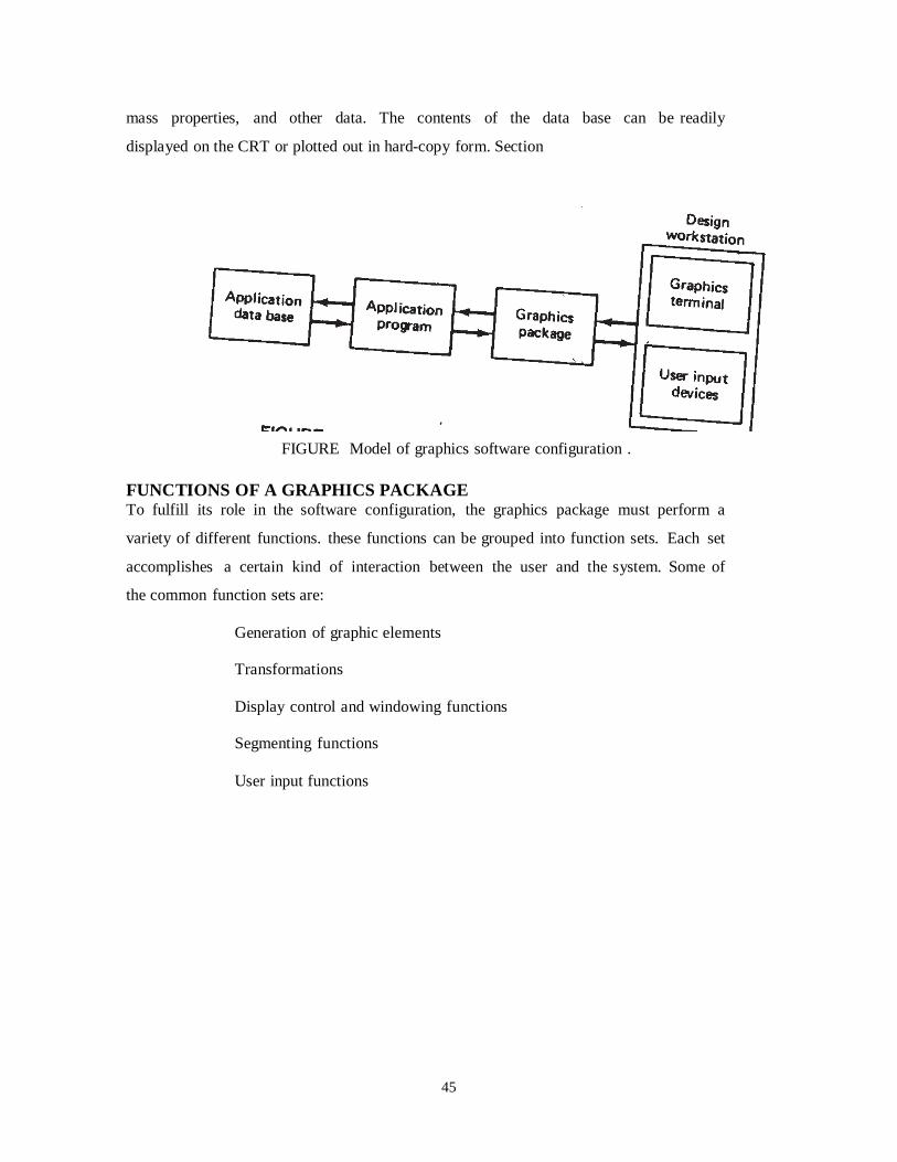
45

mass properties, and other data. The contents of the data base can be readily

displayed on the CRT or plotted out in hard-copy form. Section

FIGURE Model of graphics software configuration .

FUNCTIONS OF A GRAPHICS PACKAGE To fulfill its role in the software configuration, the graphics package must perform a

variety of different functions. these functions can be grouped into function sets. Each set

accomplishes a certain kind of interaction between the user and the system. Some of

the common function sets are:

Generation of graphic elements

Transformations

Display control and windowing functions

Segmenting functions

User input functions

46

TRANSFORMATIONS

Many of the editing features involve transformations of the graphics elements or cells

composed of elements or even the entire model. In this section we discuss the mathematics of

these transformations. Two-dimensional transformations are considered first to illustrate

concepts. Then we deal with three dimensions.

Two-dimensional transformations

To locate a point in a two-axis cartesian system, the x and y coordinates are specified. These

coordinates can be treated together as a lxl matrix: (x,y). For example, the matrix (2,

5) would be interpreted to be a point which is 2 units from the origin in the x-direction and

5 units from the origin in the y-direction.

This method of representation can be conveniently extended to define a line as a 2 x 2

matrix by giving the x and y coordinates of the two end points of the line.

The notation would be

L = xl yl

x2 y2

Using the rules of matrix algebra, a point or line (or other geometric element represented in

matrix notation) can be operated on by a transformation matrix to yield a new element.

There are several common transformations used in computer graphics. We will discuss

three transformations: translation, scaling, and rotation.

TRANSLATION.

Translation involves moving the element from one location to another. In the case of

a point, the operation would be

x' =x + m, y' = y + n

where x', y' = coordinates of the translated point

x, y = coordinates of the original point

m, n = movements in the x and y directions, respectively

In matrix notation this can be represented as

(x', y') = (x, y) + T

47

where

T = (m,n), the translation matrix

Any geometric element can be translated in space by applying Eq. to each point that

defines the element. For a line, the transformation matrix would be applied to its two end

points.

SCALING.

Scaling of an element is used to enlarge it or reduce its size. The scaling need not necessarily

be done equally in the x and y directions. For example, a circle could be transformed into an

ellipse by using unequal x and y scaling factors.

The points of an element can be scaled by the scaling matrix as follows:

(x' ,y') = (x,y)S

where

m O s the scaling matrix

O n

This would produce an alteration in the size of the element by the factor m in the x-

direction and by the factor n in the y direction. It also has the effect of repositioning the

element with respect to the cartesian system origin. If the scaling factors are less than I, the

size of the element is reduced and it is moved closer to the origin. If the scaling factors are

larger than I, the element is enlarged and removed farther from the origin.

ROTATION.

In this transformation, the points of an object are rotated about the origin by an angle O. For a

positive angle, this rotation is in the counterclockwise direction. This accomplishes rotation

of the object by the same angle, but it also moves the object. In matrix notation, the

procedure would be as follows:

(x',y') = (x,y)R

where

cos O sin O R =

sin Ocos O the rotation matrix

48

EXAMPLE 1: As an illustration of these transformations in two dimensions, consider the line

defined by

l l L =

2 4

Let us suppose that it is desired to translate the line in space by 2 units in the x direction and

3 units in the y direction. This would involve adding 2 to the current x value and 3 to the

current y value of the end points defining the line. That is,

FIGURE. Results of translation in Example 6.l.

l l 2 3 3 4

2 4 2 3 4 7

The new line would have end points at (3, 4) and (4, 7). The effect of the transformation

is illustrated in Figure 6.3.

49

Example 2: For the same original line as in Example 6.l, let us apply the scaling factor of 2 to

the line. The scaling matrix for the 2 x 2 line definition would therefore be

2 O T =

O 2

The resulting line would be determined by Eq. as follows:

l l 2 O 2 4

2 4 O 2 4 8

The new line is pictured in Figure .

Example 3: We will again use our same line and rotate the line about the origin by 3Oo. Equation

would be used to determine the transformed line where the rotation matrix would be:

FigureResults of scaling in Example .

cos 3O sin 3O O.866 O.5OO R =

sin 3O cos 3O O.5OO O.866

50

The new line would be defined as:

l l O.866O.5OO O.366 l.366

2 4 O.5O O.866 O.268 4.464

The effect of applying the rotation matrix to the line is shown in Figure.

Three-dimensional transformations

Transformations by matrix methods can be extended to three-dimensional space. We

consider the same three general categories defined in the preceding section. The same

general procedures are applied to use these transformations that were defined for the three

cases by Eqs. translation. The translation matrix for a point defined in three dimensions

would be

T = (m. n, p)

FIGURE Results of rotation in Example

and would be applied by adding the increments m, n, and p to the respective coordinates of

each of the points defining the three-dimensional geometry element.

SCALING. The scaling transformation is given by

51

m O O

S = O n O

O O p

For equal values of m, n, and p, the scaling is linear.

ROTATION. Rotation in three dimensions can be defined for each of the axes

Rotation about the z axis by an angle is accomplished by the matrix

cos sin O

Rz = sin cos O

O O l

Rotation about the y axis by the angle 6 is accomplished similarly.

cos O sin

Ry = O l O

sin O cos

Rotation about the x axis by the angle is done with an analogous

transformation matrix.

l O O

Rx = O cos sin

O sin cos

Concatenation

The previous single transformations can be combined as a sequence of transformations. This

is called concatenation, and the combined transformations are called concatenated

transformations.

During the editing process when a graphic model is being developed. the use of

concatenated transformations is quite common. It would be unusual that only a single

transformation would be needed to accomplish a desired manipulation of the image. Two

examples of where combinations of transformations would be required would be: -

Rotation of the element about an arbitrary point in the element

52

Magnifying the element but maintaining the location of one of its points in

the same location

In the first case, the sequence of transformations would be' translation to the origin, then

rotation about the origin, then translation back to the original location. In the second case,

the element would be scaled (magnified) followed by a translation to locate the desired

point as needed:-

The objective of concatenation is to accomplish a series of image manipulations

as a single-transformation. This allows the concatenated transformation to be defined

more concisely and the computation can generally be accomplished more efficiently.

Determining the concatenation of a sequence of single transformations can be fairly

straightforward if the transformations are expressed in matrix form as we have done. For

example. if we wanted to scale a point by the factor of 2 in a two dimensional system and

then rotate it about the origin by 45°, the concatenation would simply be the product of

the two transformation matrices. It is important that the order of matrix multiplication

be the same as the order in which the transformations are to be carried out.

Concatenation of a series of transformations becomes more complicated when a translation

is involved, and we will not consider this case.

53

MODELLING

WIRE-FRAME VERSUS SOLID MODELING

The importance of three-dimensional geometry

Early CAD systems were basically automated drafting board systems which displayed a two-

dimensional representation of the object being designed. Operators (e.g., the designer or

drafter) could use these graphics systems to develop the line drawing the way they wanted it

and then obtain a very high quality paper plot of the drawing. By using these systems, the

drafting process could be accomplished in less time, and the productivity of the designers

could be improved.

However, there was a fundamental shortcoming of these early systems. Although they were

able to reproduce high-quality engineering drawings efficiently and quickly, these systems

stored in their data files a two-dimensional record of the drawings. The drawings were

usually of three-dimensional objects and it was left to the human beings who read these

drawings to interpret the three-dimensional shape from the two-dimensional representation.

The early CAD systems were not capable of interpreting the three-dimensionality of the

object. It was left to the user of the system to make certain that the two-dimensional

representation was correct (e.g., hidden lines removed or dashed, etc.), as stored in the data

files.

More recent computer-aided design systems possess the capability to define objects in three

dimensions. This is a powerful feature because it allows the designer to develop a full three-

dimensional model of an object in the computer rather than a two-dimensional illustration.

The computer can then generate the orthogonal views, perspective drawings, and close-ups of

details in the object.

The importance of this three-dimensional capability in interactive computer graphics should

not be underestimated.

Wire-Frame models

Most current day graphics systems use a form of modeling called wire- frame modeling.

In the construction of the wire-frame model the edges of the objects are shown as lines. For

objects in which there are curved surfaces, contour lines can be added; as shown in

Figure, to indicate the contour. The image assumes the appearance of a frame constructed

out of wire - hence the name wire frame model.

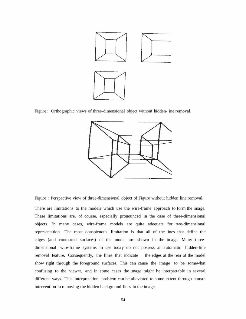
54

Figure : Orthographic views of three-dimensional object without hidden- ine removal.

Figure : Perspective view of three-dimensional object of Figure without hidden line removal.

There are limitations to the models which use the wire-frame approach to form the image.

These limitations are, of course, especially pronounced in the case of three-dimensional

objects. In many cases, wire-frame models are quite adequate for two-dimensional

representation. The most conspicuous limitation is that all of the lines that define the

edges (and contoured surfaces) of the model are shown in the image. Many three-

dimensional wire-frame systems in use today do not possess an automatic hidden-line

removal feature. Consequently, the lines that indicate the edges at the rear of the model

show right through the foreground surfaces. This can cause the image to be somewhat

confusing to the viewer, and in some cases the image might be interpretable in several

different ways. This interpretation problem can be alleviated to some extent through human

intervention in removing the hidden background lines in the image.

55

There are also limitations with the wire-frame models in the way many CAD systems

define the model in their data bases. For example, there might be ambiguity in the case of a

surface definition as to which side of the surface is solid. This type of limitation prevents

the computer system from achieving a comprehensive and unambiguous definition of

the object.

Figure : Wireframe model of F/A-l8 fighter aircraft, showing primary control curves.

Solid models An improvement over wire-frame models, both in terms of realism to the user and

definition to the computer, is the solid modeling approach. In this approach, the models are

displayed as solid objects to the viewer, with very little risk of misinterpretation. When color

is added to the image, the resulting picture becomes strikingly realistic. It is anticipated

that graphics systems with this capability will find a wide range of applications outside

computer-aided design and manufacturing. These applications will include' color illustrations

in magazines and technical publications, animation in movie films, and training simulators

(e.g., aircraft pilot training).

There are two factors which promote future widespread use of solid modelers (i.e.,

graphics systems with the capability for solid modeling). The first is the increasing

awareness among users of the limitations of wire-frame systems. As powerful as today's

56

wire-frame-based CAD systems have become, solid model systems represent a dramatic

improvement in graphics technology. The second reason is the continuing development

of computer hardware and software which make solid modeling possible. Solid modelers

require a great deal of computational power, in terms of both speed and memory, in order

to operate.

The advent of powerful, low-cost minicomputers has supplied the needed capacity to meet

this requirement. Developments in software will provide application programs which take

advantage of the opportunities offered by solid modelers. Among the possibilities

are more highly automated model building and design systems, more complete three-

dimensional engineering analysis of the models, including interference checking,

automated manufacturing planning, and more realistic production simulation models.

Two basic approaches to the problem of solid modeling have been developed:

l. Constructive solid geometry (CSG or C-rep), also called the building-

block approach

2. Boundary representation (B-rep)

The CSG systems allow the user to build the model out of solid graphic

primitives, such as rectangular blocks, cubes, spheres, cylinders, and pyramids. This

building-block approach is similar to the methods described in Section 6.4 except

that a solid three-dimensional representation of the object is produced. The most

common method of structuring the solid model in the graphics data base is to use

Boolean operations, described in the preceding section and pictured in Figure.

57

The boundary representation approach requires the user to draw the outline or boundary of

the object on the CRT screen using an electronic tablet and pen or analogous procedure. The

user would sketch the various views of the object (front, side, and top, more views if

needed), drawing interconnecting lines among the views to establish their relationship.

Various transformations and other specialized editing procedures are used to refine the model

to the desired shape. The general scheme is illustrated in Figure

The two approaches have their relative advantages and disadvantages. The C-rep systems

usually have a significant procedural advantage in the initial formulation of the

model. It is relatively easy to construct a precise solid model out of regular solid primitives

by adding, subtracting, and intersecting the components. The building-block approach also

results in a more compact file of the model in the database.

Figure 2.4: Input views of the types required for boundary representation (B-rep) .

.

58

On the other hand, B-rep systems have their relative advantages. One of them becomes

evident when unusual shapes are encountered that would not be included within the

available repertoire of the CSG systems. This kind of situation is exemplified by aircraft

fuselage and wing shapes and by automobile body styling. Such shapes would be quite

difficult to develop with the building-block approach, but the boundary representation

method is very feasible for this sort of problem.

Another point of comparison between the two approaches is the difference in the way the

model is stored in the data base for the two systems. The CSG approach stores the

model by a combination of data and logical procedures (the Boolean model). This

generally requires less storage but more computation to reproduce the model and its

image. By contrast, the B-rep system stores an explicit definition of the model

boundaries. This requires more storage space but does not necessitate nearly the same

computation effort to reconstruct the image. A related benefit of the B-rep systems is that it is

relatively simple to convert back and forth between a boundary representation and a

corresponding wire-frame model. The reason is that the model's boundary definition is similar

to the wire-frame definition, which facilitates conversion of one form to the other. This

makes the newer solid B-rep systems compatible with existing CAD systems out in the field.

Because of the relative benefits and weaknesses of the two approaches, hybrid systems

have been developed which combine the CSG and B-rep approaches. With these systems,

users have the capability to construct the geometric model by either approach, whichever

is more appropriate to the particular problem.

59

UNIT -II

GEOMETRIC MODELING

Geometry

Topology

Spatial addressability

Geometry Vs Topology

For wire frame- geometrical data

For surface model- geometrical data

For solid model- topology and geometry

Geometry is the acual dimensions that defines entities of a object

Geometry is visible to users

The geometry that defines the object shown below

Length of lines L1, L2, L3

Angle between lines

The center point P1 of semi circle

Topology or Combinational structure

It is the connectivity and association of the object entity

It determines relational information between object entities

Topology of object can be stated as below

L1 shares a vertex point with L2 & C1

L2 shares a vertex point with L1 & L3

L3 shares a ertex point with L2 & C1

L1 & L3 do not overlap

P1 lies outside the object

Example for better understanding

a) Same geometry but different topology

b) Same topology but different geometry

Spatial Addresability

A complete geometric data representation of an object is one that enables points in

space to be classified relative to the object, if it is inside or outside or on the object

Addresability

A complete geometric data representation of an object is one that enables points in space

to be classified relative to the object, if it is inside or outside or on the object This

classification is called spatial addressability.

60

3D modeling

Point location

Spatial addresability On object

Inside object

Outside Object

Wire frame Incapable of handling spatial address

Surface Incapable of handling spatial address

Solid Capable of handling spatial address

Free form surfaces

These are the surfaces which cannot be defined by any analytical techniques

Ex: Sculpture surface Surface is controlled by series of control points and boundaries

These are large number of numerical techniques available such as Brazier, Curves, Spline

surfaces and NURBS, etc

Classification of surfaces

I. Planar surfaces: a flat 2Dsurface

II. Curved surfaces :

Single curved surfaces :It s a simple curved surface obtained by rotating straight lines

around an axis Ex: cylindrical, conical, pyramid surfaces, prisms and -Double curved

surfaces: They are complex surfaces generated by complex curved lines/ surfaces

Ex: Spherical, Torous, Ellipsoid, Parabaloid, Fuselage, Automobiles, etc

A ruled surface: constructed by transiting between two or more curves by using linear

bending between each section OF SURFACE. Curve fitting methods For geometrical modeling curve fitting methods are generally used which are broadly

classified as: Interpolation techniques

Between interpolation & approximation

Interpolation Best fit/ Approximate

Curve can be made to

pass through all the

control data points for

designing curve and

surface

The curve does not pass through all the points for

designing curves and surfaces

Actual shape between

points depends on

degree of polynomial

& boundary condition

Used in computer graphics to design curves that

look good and aesthetic goal. It can also be used

to design free form surfaces, sculptures, surface

of automobiles, aerodynamic profile

Used to reconstruct

the shape of degitized

curved object

Ex: cubic spline

These techniques are preferred over

interpolation in curve design due to the added

flexibility and additional initiative fuel

Ex: Bazier curve, B- Spline

Cubic spline &

Lagrange

interpolation methods

used

Regression & least square matrix are used

61

The shape of curve is

affected greatly by

manipulating a single

data point. The nature

of tweaking is

unpredictable

It is possible to have local modification by

tweaking a single point where the behavior is

more predictable

Important properties for designing curves

Control points : data points

1. start from 0 to n

2. total n+1 points

3. Multiple values: parametric formation of a curve allows it to represent multiple

valued shapes. A curve is multi valued with respect to all coordinate systems

4. Axis of independence: - curves must be independent of coordinate systems

if any point on curve is moved by x0 then the curve rotates x0 but shape does not

change.

5. Control :- Global control: moving any control point on curve , this leads o entire

curve moves.

Ex:Bazier curve

Local control: moving control point on curve results only that point move on curve.

Ex: B- spline

6. Variation Diminishing properties : Curve should not oscillate widely away from it is

defined control pairs.

Ex: Brazier curves.

7. Versactality : depends on the number of control points. Ex: complex curve more

control points

8. Order of continuity: Continuity at joints between curves. ex:

c0, c

1, c

2

Parametric continuity condition

Data points are called control points to construct a smooth curve that passes through the

given data points, various continuity requirements can be specified at the data points to

impose various degree of smoothness of the resulting curve.

The order f continuity becomes more important where a complex curve is modeled by

several curved segments pieced together end to end. If each set of curve is described with

parametric coordinate functions of the form x=f(u), y=g(u), & l= h(u)

Whereumin≤ u ≤ umax

To ensure a smooth transition from one section of segment to the next we can impose the

following continuity condition at the joint of connecting points. Therefore, - Zero order

parametric continuity ( c0)

- First order parametric continuity ( c1)

- Second order parametric continuity (c2)

C0 continuity: zero order parametric continuity describes as c0 continuity means simply that

the curves meet i.e. values of x,y,z evaluated t umax of first curve section are equal

respectively to the values of x,y,z evaluated at uminfor the next curve section.

C1 continuity: the first order parametric continuity referred as c1 continuity means that the

first parametric derivatives ( tangent lines/ vectors) of coordinate function is function for

62

two successive curve sections are equal after joining points. Curves are same as the

intersection. First order continuity is often sufficient for digitizing drawings and for some

design applications.

C2 continuity: second order parametric continuity c2 continuity means that the both first

order and second order parametric derivates of line segment sections ( i.e. end points of firs

segment sections 2nd order parametric derivatives= start point of 2nd segment, 1st and 2nd

order parametric derivatives.) are same at the intersection.

First derivative of parametric equations of segment – end point = first order derivative

parametric equation of start point of 2nd segment.

Similarly End point of 2nd order derivative of 1st segment= start point of 2nd order

derivative of 2nd Segment 2nd order continuity is useful for setting approximation path for

camera motion for many precisions CAD requirements.

Blending function

When modeling a curve f(x) by using curve segments, we try to represent the curve as a sum

of smaller segments Ǿi(x) called blending function or basis function.

Analytical curves

Analytical curves are defined as those that can be described by analytical equations such as

lines, circles and conics. Analytical curves provide very compact forms to represent shapes

and simplify the computation of related properties such as areas and volumes

Analytical curves are not attractive to deal with interactively

Analytical curves are points, lines, arcs and circles, fillets and chambers and also conics

like parabola, hyperbola, ellipse, etc.

Synthetic curves

A synthetic curve is defined as that can be described by a set of data points( control points)

such as splines and bazier curves. Synthetic curves provide designers with greater flexibility

and control of curve shapes by changing the positions of control points. Global and local

control of a curve is possible. Synthetic curves are attractive to deal with interactively

Synthetic curves include various types of splines like cubic spline, B- spline, NURBS and

Bazier curves.

Curves

A 3D curve is an object in space that the direction only much like a thread A curve has one

degree of freedom. This means that a point on a curve can be moved in only one

independent direction Curve representation: is represented by an equation or group of

equations that has only one free variable or parameter (i.e. u)

The x,y,z coordinates of any point on the curve are determined by this free variable or

parameter

Mathematically there are 2 types of curve representatons

a) Non parameteric form: - explicit -implicit

b) Parameteric form:

-analytical

-synthetical

63

=0 i i

Parametric curve description

A parametric form curve is described by an equation or group of equations that has only one

free variable or parameter.

Surface

A surface is a 3D space in an object that has breadth and width much like a piece of cloth A

surface has two degrees of freedom. This means that a point on surface can be moved in

2independent directions The x,y,z coordinates of any point on the surface are determined by

these free variables or parameters( i.e. u & v) Mathematically there are two types of surface

description

Non parametric surface description: - implicit -explicit

Parametric surface description: -analytical -synthetic

PARAMETERIC REPRESENTATION OF SYNTHETIC CURVES

-Analytical curves are insufficient to meet the requirement of mechanical points having complex

curve shapes such as Propeller blades Aircraft wings Ship nuts Automobile bodies

The composite require free form or synthetic curve -Design of curved boundaries and surfaces

require curve representations that can be manipulated by changing data points which will create

bends and sharp turns in the shape of the curve These curves are called Synthetic curve and data

points are called control points.

-If curve passes through all the data points it is called as interpolated curve.

-The smoothness of curve is mere important requirement of synthetic curve. Most popular

synthetic curves are

- Hermit cube

- Bezier curve

- B- spline

- NURBS (Non- Uniform Rotation B- Spline)

1) Hermit cube curve (HCC)

- HCC is defined by defining 2position vectors and 2 tangent vectors at

data points

- Hermit cube curve is also called as parametric cube curve and cubic

spline

- The curve is used to interpolate given data points but not free form

curve

- The most commonly used, cubic spline is a 3D planer curve

- It is represented by cubic polynomial

- Several splines can be joined together by imposing slope continuity at

the corner points.

- The parametric equation for a cubic spline is given by

P u = 3 a u 0<u<1

64

=0

(1)

Where aiare polynomial coefficients and u is the parameter.

Expand (1)

P(u)= a0+a1u+a2u2+a3u

3

------(2)

If x,y,z are coordinates of P equation be

X(u) = a0x+a1xu+ a2xu2+a3xu

3

Y(u) = a0y+a1yu+ a2xu2+a3yu

3

Z(u) = a0x+a1xu+ a2xu2+a3zu

3

Tangent vector to the curve at any point is obtained by differentiating equation (1) wrt u

Now P’(u) = 3 ai.i.ui-1

Where 0<u<1

-- (3)

(i) Tangent vector at point P can be defined as

X’(u)= a1x+ 2a2xu+3a3xu2

Y’(u)= a1x+ 2a2xu+3a3yu2

Z’(u)= a1x+ 2a2xu+3a3zu2

The coefficients can be evaluated by applying the boundary conditions at the end

points.

Substituting boundary conditions at u=0, u=1 in equation (2) & (3) we get

P0= P(0)= a0

65

P1= P(1)= a0+ a1+ a2+ a3

P’0= P’(0)= a1

P’1= P’(1)= a1+ 2a2+ 3a3

Solving these equations simultaneously for coefficients, we get

a0= P0,

a1 = P0

a2= 3(P1- P0) – ( 2P’0+ P’1)

a3= -2(P1- P0) + P’0+ P’1

Parametric Cubic Curves

In order to assure C1 continuity at two extremities, our functions must be of at least degree

Here's what a parametric cubic spline function looks like: Alternatively, it can be

written in matrix form:

Solving for Coefficients

An Illustrative Example

Cubic Hermite Splines:

66

The Gradient of The Gradient of a Cubic Spline

The Hermite Specification as a Matrix Equation

Solve for the Hermite Coefficients

67

The Hermite Specification as a Matrix Equation

Spline Basis and Geometry Matrices

68

Resulting Cubic Hermite Spline Equation

Bézier Curves Another Spline class that has more intuitive controls

A Cubic Bézier Spine has four control points, two of which are knots.

Bezier spline is a way to define a curve by sequence of two end points and one or more control points which control the curve. Two end points are called Anchor Points. The bezier splines with two control points are called Cubic Bezier Spline.

69

Coefficients for Cubic Bezier Splines It just so happens that the knot gradients of a Bezier Spline can be expressed in terms of

the adjacent control points:

Bezier Blending Functions The reasonable justification for Bezier spline basis can only be approached by considering its

blending functions:

70

This family of polynomials (called order-3 Bernstein polynomials) have the following unique

properties:

They are all positive in the interval [0, 1] Their sum is equal to 1

71

B Spline functions

Bi(u) = (u^3)/6Bi-1(u) = (-3*(u^3) + 3*(u^2) + 3*u +1)/6 Bi-2(u) = (3*(u^3) - 6*(u^2) +4)/6

Bi-3(u) = (1 - u)^3/6

Bi(u) = (u^3)/6Bi-1(u) = (-3*((u-1)^3) + 3*((u-1)^2) + 3*(u-1) +1)/6

Bi-2(u) = (3*((u-2)^3) - 6*((u-2)^2) +4)/6

Bi-3(u) = (1 - (u-3))^3/6

72

Bi(u) = (u^3)/6

Bi-1(u) = (-3*((u-1)^3) + 3*((u-1)^2) + 3*(u-1) +1)/6

Bi-2(u) = (3*((u-2)^3) - 6*((u-2)^2) +4)/6

Bi-3(u) = (1 - (u-3))^3/6

B(u) = Bi(u) when 0 <= u < 1,

Bi-1(u) when 1 <= u < 2, Bi-

2(u) when 2 <= u < 3, Bi-3(u)

when 3 <= u < 4

Bi(u) = (u^3)/6 Bi1(u) = (-3*((u-1)^3) + 3*((u-1)^2) + 3*(u-1) +1)/6

Bi2(u) = (3*((u-2)^3) - 6*((u-2)^2) +4)/6

Bi3(u) = (1 - (u-3))^3/6

B(u) = Bi(u) when 0 <= u < 1, Bi1(u)

when 1 <= u < 2,

73

Bi2(u) when 2 <= u < 3,

Bi3(u) when 3 <= u < 4

B1(u)

=

B(u-1)

B2(u)

B3(u)

B4(u)

=

=

=

B(u-2)

B(u-3)

B(u-4)

74

Algebraic and geometric form:

Surface entities:

Parametric space of surface , subdividing:

A parametric surface is a surface in the Euclidean space which is defined by a parametric

equation with two parameters Parametric representation is a very general way to specify a surface,

as well as implicit representation. Surfaces that occur in two of the main theorems of vector

calculus, Stokes' theorem and the divergence theorem, are frequently given in a parametric form.

The curvature and arc length of curves on the surface, surface area, differential geometric invariants

such as the first and second fundamental forms, Gaussian, mean, and principal curvatures can all be

computed from a given parameterization.

We can represent a surface as a series of grid points inside its bounding curves. Surfaces can be in

two-dimensional space (planar) or in three-dimensional space (general surfaces). Surface can be

described using non-parametric or parametric equations Surfaces can be represented by equations to

pass through all the data points (fitting) or have patches of them connected at the data points.

Geometric Shape:

A geometric shape is the geometric information which remains

when location, scale, orientation and reflection are removed from the description of a geometric

object. That is, the result of moving a shape around, enlarging it, rotating it, or reflecting it in a

mirror is the same shape as the original, and not a distinct shape.

Objects that have the same shape as each other are said to be similar. If they also have the same

scale as each other, they are said to be congruent.

Many two-dimensional geometric shapes can be defined by a set

of points or vertices and lines connecting the points in a closed chain, as well as the resulting interior

points. Such shapes are called polygons and include triangles, squares, and pentagons. Other shapes

may be bounded by curves such as the circle or the ellipse.

75

Subdividing:

A parametric surface is a surface in the Euclidean space which is defined by

aparametric equation with two parameters. Parametric representation is a very general way to

specify a surface, as well as implicit representation.

Cylindrical Surface:

A cylindrical surface whose generatrix is parallel to one of the coordinate axes and whose directrix

is a curve in the coordinate plane that is perpendicular to the generatrix, has the same equation as the

directrix. For example, if the directrix is the ellipse. in the x-y plane, the equation of the ellipse as

In the x-y plane, the equation of the cylinder is Cylinder. (1) A cylindrical surface (2) Suppose we

are given two parallel planes and two simple closed curves C1 and C2 in these planes for which lines

joining corresponding points of C1 and C2 are parallel to a given line L. A cylinder is a closed

surface consisting of two bases which are plane regions bounded by such curves C1 and C2 and

a lateral surface which is the union of all line segments joining corresponding points of C1 and C2.

Each of the curves C1 and C2 is a directrix of the cylinder and the line segments joining

corresponding points of C1 and C2 are elements (or generators or rulings). The cylinder

is circular or elliptic if a directrix is a circle or an ellipse, respectively. Sometimes a circular

cylinder is defined to be a cylinder whose intersections with planes perpendicular to the elements are

circles. The cylinder is a right cylinder or an oblique cylinder according as L is perpendicular to the

planes or not perpendicular to the planes. The altitude of a cylinder is the perpendicular distance

between the planes containing the bases and a right section is the intersection of the cylinder and a

plane perpendicular to the elements that crosses the cylinder between the bases.

76

Ruled surface

Ruled Surfaces are surfaces that are generated using two curves with a straight line connecting each

curve. The two driving curves can be 3D Curves or existing edges of parts or other surfaces. Ruled

Surface, Ruled Surface to Point, and Ruled Surface to Face Examples.

A ruled surface can be described as the set of points swept by a moving straight line. For example, a

cone is formed by keeping one point of a line fixed whilst moving another point along a circle. A

surface is doubly ruled if through every one of its points there are two distinct lines that lie on the

surface.

77

Surface of revolution spherical surface:

A surface of revolution is generated by revolving a given curve about an axis. The given

curve is a profile curve while the axis is the axis of revolution..

Many commonly seen and useful surfaces are surfaces of revolution (e.g., spheres,

cylinders, cones and tori).

Sphere:

A sphere is obtained by revolving a sei-circle about the axis of revolution. In the curve

system, this semi-circle must be in the xz-plane and the axis of revolution must be the z-

axis.

78

79

UNIT III

GROUP TECHNOLOGY

INTRODUCTION

Group technology (abbreviated GT) is a manufacturing philosophy in which similar parts are

identified and grouped together to take advantage of their similarities in

manufacturing and design. Similar parts are arranged into part families. For example, a

plant producing lO,OOO different part numbers may be able to group the vast majority of

these parts into 5O or 6O distinct families. Each family would possess similar design and

manufacturing characteristics. Hence, the processing of each member of a given family

would be similar, and this results in manufacturing efficiencies. These efficiencies are

achieved in the form of reduced setup times, lower in-process inventories, better

scheduling, improved tool control, and the use of standardized process plans. In some plants

where GT has been implemented, the production equipment is arranged into machine groups,

or cells, in order to facilitate work flow and parts handling.

In product design, there are also advantages obtained by grouping parts into families. For

example, a design engineer faced with the task of developing a new part design must either

start from scratch or pull an existing drawing from the files and make the necessary changes

to conform to the requirements of the new part.

The problem is that finding a similar design may be quite difficult and time consuming. For a

large engineering department, there may be thousands of drawings in the files, with no

systematic way to locate the desired drawing. As a consequence, the designer may decide

that it is easier to start from scratch in developing the new part. This decision is replicated

many times over in the company, thus consuming valuable time creating duplicate or near-

duplicate part designs. If an effective design- retrieval system were available, this waste

could be avoided by permitting the engineer to determine quickly if a similar part already

exists. A simple change in an existing design would be much less time consuming than starting

from scratch. This design-retrieval system is a manifestation of the group technology principle

applied to the design function. To implement such a system, some form of parts classification

and coding is required.

80

Parts classification and coding is concerned with identifying the similarities among parts and

relating these similarities to a coding system. Part similarities are of two types: design

attributes (such as geometric shape and size), and manufacturing attributes (the sequence of

processing steps required to make the part). While the processing steps required to

manufacture a part are usually correlated with the part's design attributes, this is not always the

case. Accordingly, classification and coding systems are often devised to allow for

differences between a part's design and its manufacture.

Whereas a parts classification and coding system is required in a design- retrieval system,

it can also be used in computer-aided process planning (CAPP). Computer-aided process

planning involves the automatic generation of a process plan (or route sheet) to

manufacture the part. lbe process routing is developed by recognizing the specific attributes

of the part in question and relating these attributes to the corresponding manufacturing

operations.

In the present chapter we develop the topics of group technology and p classification and

coding. In the following chapter we present a discussion of computer-aided process

planning and several related issues. Group technology and parts classification and coding are

based on the concept of a part family.

3.2 PART FAMILIES A part family is a collection of parts which are similar either because of geometric shape

and size or because similar processing steps are required in their manufacture. The parts

within a family are different, but their similarities are close enough to merit their

identification as members of the part family. Figures show two part families. The two parts

shown in Figure are similar from design viewpoint but quite different in terms of

manufacturing. The parts shown in Figure might constitute a part family in manufacturing, but

their geometry characteristics do Dot permit them to be grouped as a design part family.

81

The part family concept is central to design-retrieval systems and modify current

computer-aided process planning schemes. Another important manufacturing

Two parts of identical shape and size but different manufacturing requirements.

Thirteen parts with similar manufacturing process requirements but different design attributes.

Advantage derived from grouping workparts into families can be explained with reference

to Figures. Figure shows a process-type layout for batch production in a machine shop.

The various machine tools are arranged by function. There is a lathe section, milling

machine section, drill press section, and so on. During the machining of a given part, the

workpiece must be moved between sections, with perhaps the same section being visited

several times. This results in a significant amount of material handling, a large in-process

inventory, usually more setups than necessary, long manufacturing lead times, and high cost.

Figure shows a production shop of supposedly equivalent capacity, but with the machines

arranged into cells. Each cell is organized to specialize in the manufacture of a particular

part family. Advantages are gained in the form of

82

Process-type layout.

Group technology layout.

reduced workpiece handling, lower setup times, less in-process inventory, less floor

space, and shorter lead times. Some of the manufacturing cells can be designed to

form production flow lines, with conveyors used to transport workparts between

machines in the cell. The biggest single obstacle in changing over to group technology

from a traditional production shop is the problem of grouping parts into families. There

are three general methods for solving this problem. All three methods are

time consuming and involve the analysis of much data by properly trained personnel.

The three methods are:

2. Production flow analysis (PFA)

3. Parts classification and coding system

83

The visual inspection method is the least sophisticated and least expensive method. It involves

the classification of parts into families by looking at either the physical parts or photographs

and arranging them into similar groupings. This method is generally considered to be the

least accurate of the three.

The second method, production flow analysis, was developed by J. L. Burbidge. PFA is a

method of identifying part families and associated machine tool groupings by analyzing the

route sheets for parts produced in a given shop. It groups together the parts that have similar

operation sequences and machine routings. The disadvantage of PF A is that it accepts the

validity of existing route sheets, with no consideration given to whether these process plans

are logical or consistent. The production flow analysis approach does not seem to be used

much at all in the United States.

The third method, parts classification and coding, is the most time consuming and

complicated of the three methods. However, it is the most frequently applied method and is

generally recognized to be the most powerful of the three.

3.3 PARTS CLASSIFICATION AND CODING This method of grouping parts into families involves an examination of the individual design

and/or manufacturing attributes of each part. The attributes of the part are uniquely

identified by means of a code number. This classification and coding may be carried out

on the entire list of active parts of the firm, or a sampling process may be used to establish the

part families. For example, parts produced in the shop during a certain given time period could

be examined to identify part family categories. The trouble with any sampling procedure is the

risk that the sample may be unrepresentative of the entire population. However, this risk may

be worth taking, when compared to the relatively enormous task of coding all the company's

parts.

Many parts classification and coding systems have been developed throughout the

world, and there are several commercially available packages being sold to industrial

concerns. It should be noted that none of them has been universally adopted. One of the

reasons for this is that a classification and coding system should be custom-engineered for a

given company or industry. One system may be best for one company while a different

system is more suited to another company.

84

TABLE Design and Manufacturing Part Attributes Typically Included in a Group Technology

Classification System

Part design attributes

Basic external shape Major dimensions

Basic internal shape Minor dimensions

Length/diameter ratio Tolerances Material

type Surface finish

Part function

Part manufacturing attributes

Major process Operation sequence

Minor operations Production time

Major dimensions Batch size

Length/diameter ratio Annual production

Surface finish Fixtures needed

Machine tool Cutting tools

Design systems versus manufacturing systems Parts classification and coding systems divide themselves into one of three general categories:

l. Systems based on part design attributes

2. Systems based on part manufacturing attributes

3. Systems based on both design and manufacturing attributes Systems in the first category are useful for design retrieval and to promote design

standardization. Systems in the second category are used for computer-aided process planning,

tool design, and other production-related functions. The third category represents an

attempt to combine the functions and advantages of the other two systems into a single

classification scheme. The types of design and manufacturing parts attributes typically

included in classification schemes are listed in Table. It is clear that there is a certain amount

of overlap between the design and manufacturing attributes of a part.

Coding system structure

85

A parts coding scheme consists of a sequence of symbols that identify the part' design

and/or manufacturing attributes. The symbols in the code can be al numeric, all

alphabetic, or a combination of both types. However, most of the common classification

and coding systems use number digits only. There are basic code structures used in group

technology applications:

l. Hierarchical structure

2. Chain-type structure

3. Hybrid structure, a combination of hierarchical and chain-type structures

With the hierarchical structure, the interpretation of each succeeding symbol depends on the

value of the preceding symbols. Other names commonly used for this structure are monocode

and tree structure. The hierarchical code provides a relatively compact structure which

conveys much information about the part in a limited number of digits.

In the chain-type structure, the interpretation of each symbol in the sequence is fixed and

does not depend on the value of preceding digits. Another name commonly given to

this structure is polycode. The problem associated with polycodes is that they tend to be

relatively long . On the other hand, the use of a polycode allows for convenient identification of

specific part attributes. This can be helpful in recognizing parts with similar processing

requirements.

To illustrate the difference between the hierarchical structure and the chain type structure,

consider a two-digit code, such as l5 or 25. Suppose that the first digit stands for the general

part shape. The symbol l means round workpart and 2 means flat rectangular geometry. In

a hierarchical code structure, the interpretation of the second digit would depend on the

value of the first digit. If preceded by l, the 5 might indicate some length/diameter ratio,

and if preceded by 2, the 5 might be interpreted to specify some overall length. In the

chain-type code structure, the symbol 5 would be interpreted the same way regardless of the

value of the first digit. For example, it might indicate overall part length, or whether the part is

rotational or rectangular.

Most of the commercial parts coding systems used in industry are a combination of the two

pure structures. The hybrid structure is an attempt to achieve the best features of

monocodes and polycodes. Hybrid codes are typically constructed as a series of short

polycodes. Within each of these shorter chains, the digits are independent, but one or more

symbols in the complete code number are used to classify the part population into groups, as

86

in the hierarchical structure. This hybrid coding seems to best serve the needs of both design

and production.

3.5 THREE PARTS CLASSIFICATION AND CODING SYSTEMS When implementing a parts classification and coding system, most companies elect

to purchase a commercially available package rather than develop their own. Inyong Ham

recommends that the following factors be considered in selecting a parts coding and

classification system:

Objective. The prospective user should first define the objective for the system. Will it be

used for design retrieval or part-family manufacturing or both?

Scope and application. What departments in the company will use the system? What

specific requirements do these departments have? What kinds of information must be coded?

How wide a range of products must be coded? How complex are the parts, shapes,

processes, tooling, and so forth?

Costs and time. The company must consider the costs of installation, training, and

maintenance for their parts classification and coding system.

Will there be consulting fees, and how much? How much time will be required to install

the system and train the staff to operate and maintain it? How long will it be before the benefits

of the system are realized?

Adapability to other systems. Can the classification and coding system be readily adapted

to the existing company computer systems and data bases? Can it be readily integrated with

other existing company procedures, such as process planning, NC programming, and

production scheduling?

Management problems. It is important that all involved management personnel be

informed and supportive of the system. Also, will there be any problems with the union?

Will cooperation and support for the system be obtained from the various departments

involved?

In the sections below, we review three parts classification and coding systems which are

widely recognized among people familiar with GT:

i . Opitz system, 2. MICLASS system and 3. CODE system

3.6.1 The Opitz classification system

87

This parts classification and coding system was developed by H. Opitz of the University

of Aachen in West Germany. It represents one of the pioneering efforts in the group

technology area and is perhaps the best known of the classification and coding schemes.

The Opitz coding system uses the following digit sequence:

l2345 6789 ABCD

The basic code consists of nine digits, which can be extended by adding four more digits. The

first nine digits are intended to convey both design and manufacturing data. The general

interpretation of the nine digits is indicated in Figure. The first five digits, l2345, are called

the "form code" and describe the primary design attributes of the part. The next four digits,

6789, constitute the supplementary code.

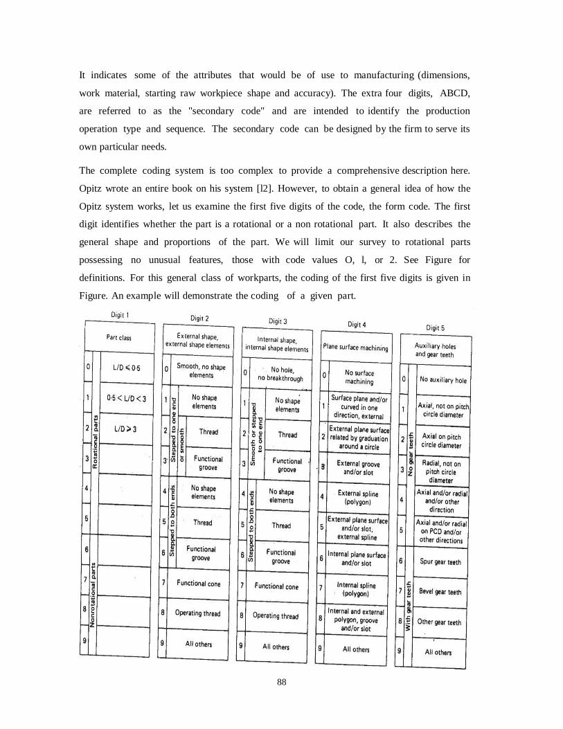
88

It indicates some of the attributes that would be of use to manufacturing (dimensions,

work material, starting raw workpiece shape and accuracy). The extra four digits, ABCD,

are referred to as the "secondary code" and are intended to identify the production

operation type and sequence. The secondary code can be designed by the firm to serve its

own particular needs.

The complete coding system is too complex to provide a comprehensive description here.

Opitz wrote an entire book on his system [l2]. However, to obtain a general idea of how the

Opitz system works, let us examine the first five digits of the code, the form code. The first

digit identifies whether the part is a rotational or a non rotational part. It also describes the

general shape and proportions of the part. We will limit our survey to rotational parts

possessing no unusual features, those with code values O, l, or 2. See Figure for

definitions. For this general class of workparts, the coding of the first five digits is given in

Figure. An example will demonstrate the coding of a given part.

89

3.6.2 The MICLASS System

MICLASS stands for Metal Institute Classification System and was developed by TNO,

the Netherlands Organization for Applied Scientific Research. It was started in Europe about five

years before being introduced in the United States in l974. Today, it is marketed in the United

States by the Organization for Industrial Research in Waltham, Massachussets. The MICLASS

system was developed to help automate and standardize a number of design, production,

and management functions. These include:

Standardization of engineering drawings

Retrieval of drawings according to classification number

Standardization of process routing

Automated process planning

Selection of parts for processing on particular groups of machine tools

Machine tool investment analysis

The MICLASS classification number can range from l2 to 3O digits. The first l2 digits are

a universal code that can be applied to any part. Up to l8 additional digits can be used to

code data that are specific to the particular company or industry. For example, lot size,

piece time, cost data, and operation sequence might be included in the l8 supplementary

digits.

The workpart attributes coded in the first l2 digits of the MICLASS number are as follows:

lst digit Main shape

2nd and 3rd digits Shape elements

4th digit Position of shape elements

5th and 6th digits Main dimensions

7th digit Dimension ratio

8th digit Auxiliary dimension

9th and lOth digits Tolerance codes

llth and l2th digits Material codes

90

3.6.4 The CODE system The CODE system is a parts classification and coding system developed and marketed by

Manufacturing Data Systems, Inc. (MDSI), of Aim Arbor, Michigan. Its most universal

application is in design engineering for retrieval of part design data, but it also has

applications in manufacturing process planning, purchasing, tool design, and inventory

control.

The CODE number has eight digits. For each digit there are l6 possible values (zero

through 9 and A through F) which are used to describe the part's design and manufacturing

characteristics. The initial digit position indicates the basic geometry of the part and is

called the Major Division of the CODE system. This digit would be used to specify whether

the shape was a cylinder, flat piece, block, or other. The interpretation of the remaining

seven digits depends on the value of the first digit, but these remaining digits form a

chain-type structure. Hence the CODE system possesses a hybrid structure.

BENEFITS OF GROUP TECHNOLOGY

Although group technology is expected to be an important principle in future

production plants, it has not yet achieved the widespread application which might be

expected. There are several reasons for this. First, as we have already indicated, there is

the problem of rearranging the machines in the plant into GT cells. Many companies have

been inhibited from adopting group technology because of the expense and disruption

associated with this transition to GT machine cells. Second, there is the problem of

identifying part families among the many components produced in the plant. Usually

associated with this problem is the expense of parts classification and coding. Not only is this

procedure expensive, but it also requires a considerable investment in time and personnel

resources. Managers often feel that these limited resources can better be allocated to

other projects than group technology with its uncertain future benefits. Finally, it is

common for companies to encounter a general resistance among its operating personnel

when changeover to a new system is contemplated.

When these problems are solved and group technology is applied, the company will

typically realize benefits in the following areas:

91

Product design

Tooling and setups

Materials handling

Production and inventory control

Employee satisfaction

Process planning procedures

92

COMPUTER-AIDED PROCESS PLANNING

THE PLANNING FUNCTION This chapter examines several process planning functions which can be implemented by

computer systems. Process planning is conerned with determining the sequence of

individual manufacturing operations needed to produce a given part or product. The

resulting operation sequence is documented on a form typically referred to as a route

sheet. The route sheet is a listing of the production operations and associated machine tools

for a workpart or assembly.

Closely related to process planning are the functions of determining appropriate

cutting conditions for the machining operations and setting the time standards for the

operations. All three functions-planning the process, determining the cutting conditions,

and setting the time standards-have traditionally been carried out as tasks with a very high

manual and clerical content. They are also typically routine tasks in which similar or even

identical decisions are repeated over and over. Today, these kinds of decisions are being made

with the aid of computers. In the first four sections of this chapter we consider the process

planning function and how computers can be used to perform this function.

Traditional process planning There are variations in the level of detail found in route sheets among different

companies and industries. In the one extreme, process planning is accomplished by

releasing the part print to the production shop with the instructions make to drawing. Most

firms provide a more detailed list of steps describing each operation and identifying each

work center. In any case, it is traditionally the task of the manufacturing engineers or

industrial engineers in an organization to write these process plans for new part designs to be

produced by the shop. The process planning procedure is very much dependent on the

experience and judgment of the planner. It is the manufacturing engineer's responsibility to

determine an optimal routing for each new part design. However, individual engineers

each have their own opinions about what constitutes the best routing. Accordingly, there are

differences among the operation sequences developed by various planners. We can

illustrate rather dramatically these differences by means of an example.

In one case cited, a total of 42 different routings were developed for various sizes of a

relatively simple part called an "expander sleeve." There were a total of 64 different sizes and

93

styles, each with its own part number. The 42 routings included 2O different machine

tools in the shop. The reason for this absence of process standardization was that many

different individuals had worked on the parts: 8 or 9 manufacturing engineers, 2 planners, and

25 NC part programmers. Upon analysis, it was determined that only two different routings

through four machines were needed to process the 64 part numbers. It is clear that there are

potentially great differences in the perceptions among process planners as to what

constitutes the "optimal" method of production.

In addition to this problem of variability among planners, there are often difficulties in

the conventional process planning procedure. New machine tools in the factory render old

routings less than optimal. Machine breakdowns force shop personnel to use temporary

routings, and these become the documented routings even after the machine is repaired.

For these reasons and others, a significant proportion of the total number of process

plans used in manufacturing are not optimal.

Automated process planning Because of the problems encountered with manual process planning, attempts have

been made in recent years to capture the logic, judgment, and experience required for

this important function and incorporate them into computer programs. Based on the

characteristics of a given part, the program automatically generates the manufacturing

operation sequence. A computer-aided process planning (CAPP) system offers the potential

for reducing the routine clerical work of manufacturing engineers. At the same time, it

provides the opportunity to generate production routings which are rational, consistent, and

perhaps even optimal. Two alternative approaches to computer-aided process planning

have been developed. These are:

l. Retrieval-type CAPP systems (also called variant systems)

2. Generative CAPP systems

The two types are described in the following two sections.

RETRIEVAL - TYPE PROCESS PLANNING SYSTEMS Retrieval-type CAPP systems use parts classification and coding and group technology as a

foundation. In this approach, the parts produced in the plant are grouped into part

families, distinguished according to their manufacturing characteristics. For each part

family, a standard process plan is established. The standard process plan is stored in

94

computer files and then retrieved for new workparts which belong to that family. Some

form of parts classification and coding system is required to organize the computer files and

to permit efficient retrieval of the appropriate process plan for a new workpart. For some new

parts, editing of the existing process plan may be required. This is done when the

manufacturing requirements of the new part are slightly different from the standard. The

machine routing may be the same for the new part, but the specific operations required at each

machine may be different. The complete process plan must document the operations as well

as the sequence of machines through which the part must be routed. Because of the

alterations that are made in the retrieved process plan, these CAPP systems are sometimes also

called by the name' 'variant system." Figure will help to explain the procedure used in a

retrieval process planning system. The user would initiate the procedure by entering the

part code number at a computer terminal. The CAPP program then searches the part

family matrix file to determine if a match exists. If the file contains an identical code

number, the standard machine routing and operation sequence are retrieved from the respective

computer files for display to the user. The standard process plan is examined by the

user to permit any necessary editing of the plan to make it compatible with the new

part design. After editing, the process plan formatter prepares the paper document in the

proper form.

If an exact match cannot be found between the code numbers in the computer file and

the code number for the new part, the user may search the machine routing file and the

operation sequence file for similar parts that could be used to develop the plan for the new

part. Once the process plan for a new part code number has been entered, it becomes the

standard process for future parts of the same classification.

95

system.

Information flow in a retrieval-type computer-aided process planning

96

In Figure the machine routing file is distinguished from the operation sequence file to

emphasize that the machine routing may apply to a range of different part families and code

numbers. It would be easier to find a match in the machine routing file than in the operation

sequence file. Some CAPP retrieval sys• terns would use only one such file which would

be a combination of operation sequence file and machine routing file.

The process plan formatter may use other application programs. These could include

programs to compute machining conditions, work standards, and standard costs. Standard

cost programs can be used to determine total product costs for pricing purposes.

A number of retrieval-type computer-aided process planning systems have been developed.

These include MIPLAN, one of the MICLASS modules [6,2O] the CAPP system developed

by Computer-Aided Manufacturing-International [l], COMCAPP V by MDSI, and systems

by individual companies [lO]. We will use MIPLAN as an example to illustrate these

industrial systems.

GENERATIVE PROCESS PLANNING SYSTEMS Generative process planning involves the use of the computer to create an individual process

plan from scratch, automatically and without human assistance. The computer would

employ a set of algorithms to progress through the various technical and logical decisions

toward a final plan for manufacturing. Inputs to the ~ tern would include a comprehensive

description of the workpart. This may involve the use of some form of part code number to

summarize the workpart data, but does not involve the retrieval of existing standard plans.

Instead, the general CAPP system synthesizes the design of the optimum process sequence,

based an analysis of part geometry, material, and other factors which would

influence manufacturing decisions.

In the ideal generative process planning package, any part design could presented to the

system for creation of the optimal plan. In practice, cu generative- type systems are far

from universal in their applicability. They ter fall short of a truly generative capability, and

they are developed for a some limited range of manufacturing processes. We will

illustrate the generative process planning approach by means system called GENPLAN

developed at Lockheed-Georgia Company

BENEFITS OF CAPP

97

Whether it is a retrieval system or a generative system, computer-aided process

planning offers a number of potential advantages over manually oriented process

planning.

l. Process rationalization. Computer-automated preparation of operation routings is more

likely to be consistent, logical, and optimal than its manual counterpart. The process

plans will be consistent because the same computer software is being used by all

planners. We avoid the tendency for drastically different process plans from different

planners. The process plans tend to be more logical and optimal because the company

has presumably incorporated the experience and judgment of its best manufacturing

people into the process planning computer software.

2. Increased productivity of process planners. With computer-aided process planning, there

is reduced clerical effort, fewer errors are made, and the planners have immediate access

to the process planning data base. These benefits translate into higher productivity of the

process planners. One system was reported to increase productivity by 6OO% in the process

planning function [lO].

3. Reduced turnaround time. Working with the CAPP system, the process planner is able to

prepare a route sheet for a new part in less time compared to manual preparation. "Ibis

leads to an overall reduction in manufacturing lead time.

4. Improved legibility. The computer-prepared document is neater and easier to read than

manually written route sheets. CAPP systems employ standard text, which facilitates

interpretation of the process plan in the factory.

5. Incorporation of other application programs. The process planning system can be

designed to operate in conjunction with other software packages to automate many of

the time-consuming manufacturing support functions.

Mono code or Hierarchical code

The structure of these codes is like a tree in which each symbol is qualified by the

preceding characters. Figure 7.1 depicts the monocode generation scheme. The first digit

(from 0 to 9) divides the set of parts into major groups such as sheet metal parts,

machined parts, purchased parts, and raw materials, and so forth. The second subsequent digits

further partition the set into subgroups for each of these groups. For example, the second

98

digit partitions the machined parts into rotational (0) and nonrotational (1) parts. Consider a

code 100 in figure 7.1. It represents a machined rotational part with a length to diameter ratio of

less than 0.5. The digit 1 in the first place of code has different meaning and different

information. Therefore, the digits in a monocode cannot be interpreted independently; the

interpretation depends on the information contained in the preceding symbol.

Advantage:

It can represent a large amount of information with very few code positions. The hierarchical nature

of the code makes it useful for storage and retrieval of design related information such as

geometry, material, and size as depicts in figure7.1.

Disadvantage:

A drawback is related to the complexity of the coding system. The applicability of these codes in

manufacturing is limited, as it is difficult to cover information on manufacturing sequences in

hierarchical manner.

Total parts

population

Sheet metal

parts

0

All machined

parts

1

Purchased

components

3 Raw

Rotational-

machined parts

0

Nonrotational- machined parts

1

0<L/D<0.5

0

0.5<L/D<1

1

L/D>10

9

0<L/W<1

0

1<L/W<3

1

materials L/W>8

9 9

Figure Example of Monocode.

Chain code or Poly code

In polycode the code symbols are independent of each other. Each digit in specific location the

code represents a distinct bit of information. A chain-structured coding scheme is presented.

Numeral 3 in the third position always means axial and cross hole no matter what numbers are

given to position 1 and 2.

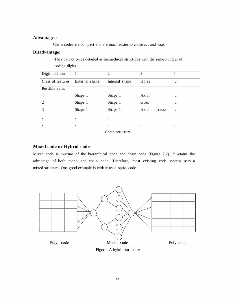
99

Advantages:

Chain codes are compact and are much easier to construct and use.

Disadvantage:

They cannot be as detailed as hierarchical structures with the same number of

coding digits.

Digit position 1 2 3 4

Class of features External shape Internal shape Holes …

Possible value

1

Shape 1

Shape 1

Axial

…

2 Shape 1 Shape 1 cross …

3 Shape 1 Shape 1 Axial and cross …

. . . . .

. . . . .

Chain structure

Mixed code or Hybrid code

Mixed code is mixture of the hierarchical code and chain code (Figure 7.2). It retains the

advantage of both mono and chain code. Therefore, most existing code system uses a

mixed structure. One good example is widely used optiz code

Poly code Mono code Poly code

Figure: A hybrid structure

100

Group Technology Coding Systems

Too much information regarding the components sometimes makes the decision very

difficult proposition. It would be better to provide a system with an abstract kind of thing, which

can summarize the whole system with the necessary information without giving great

details.

Group technology (GT) is a fitting tool for this purpose. Coding, a GT technique, can be used

to model a component with necessary information. When constructing a coding system for

a component‘s representation, there are several factors need to be considered. They include

The population of components (i.e. rotational, prismatic, deep drawn, sheet metal, and so on)

Detail in the code. The code structure. The digital representation (i.e. binary, octal, decimal,

alphanumeric, hexadecimal, and so on).In component coding, only those features are

included which are variant in nature. When a coding scheme is designed the two criteria

need to be fulfilled (1) unambiguity (2) completeness. We can define coding as a function

of F that maps components from a population space P into a coded space C (Figure 7.3).

Unambiguity of a code can be defined (for component j) as

j P only one i C i = F (j)... (1)

Completeness can be defined as j P i C i = F (j)... (2)

Population

space

H P

Code

space

C

Figure: Mapping from a population space to a code space

The two properties suggest that each component in a population has its own unique code

101

However, if two codes are complete and unambiguous, the one having more conciseness is

opted whereas a longer code is normally necessary whenever more detail is required e.g. in

basic optiz code system and the KK-3, former one uses 5 digits to describe the shape of the

component. 5 digits can represent 105

combinations. With this set, it is quite difficult to show all

the details of a component. So, KK-3 of Japan (Japan society, 1980), which has 21 digits and

contains multiple digits for single feature, and MICLASS of TNO (Houtzeel and

Schilperoort, 1976), which has a 12-digit code, is used.

Code contents

When using a code to represent an engineering design, it is important that it represents the

basic features of the design such as shape, size, tolerance, critical dimensions, material,

and so on. For process planning, it is desired to have codes that can distinguish unique production

families. Because a coding system transforms the properties and requirements of a design into a

code, the aforementioned informations must be provided to the process planning system.

The length of a part code dictates the detail that is captured by the code. In general, the

longer the code, the more detail that can be extracted. However, length and details of the code

depend on the specific application, in industrial use for product mix.

The optiz system

The Optiz coding is most likely the best-known coding system. It was developed by H. optiz

of the Aachen Tech University in West Germany. The code uses a hybrid structure. However,

except the first digit, it resembles a chain structure more closely.

It has following advantages over the existing system

It is nonproprietary.

It is widely used.

It provides a basic framework for understanding the classification and coding

process.

It can be applied to machined parts, non-machined parts, and purchased parts.

It considers both design and manufacturing information.

The optiz code consists of a form code and supplementary code (Figure 7.4). The form code

can represent parts of the following variety: long, short, cubic, flat, rotational etc. A

102

L/D

0.5

0.5

< L

/D<

3

L/D

3

Wit

h d

evia

tio

n

L/D

2

Wit

h d

evia

tio

n

L/D

>2

Spe

cial

A/B

3

A/C

4

A/B

>3

A/B

3

A/C

< 4

Spec

ial

dimension ratio is further used in classifying the geometry: the length/diameter ratio is used

to classify the rotational components and the length/height ratios are used to classify

Nonrotational components. The attributes of rotational parts are described as shown in table

7.2. The optiz form code uses five digits that focuse on 1) component class 2) basic shape 3)

rotational-surface machining 4) plane surface machining 5) auxiliary holes, gear teeth, and

forming. A supplementary code is a polycode consisting four digits is usually appended to the

Optiz system.

Digit 1

Part class

0 1 2 3 4 5 6 7 8 9

Rotational Nonrotational

Digit 2 Main shape

External shape

element

Main

shape

Main

shape

Digit 3 Rotational machining

Digit 4

Plane surface machining

Digit 5 Additional holes

Teeth and forming

Internal shape

element

Machining of

plane surface

Other holes

and teeth

Rotational

machining

Machining of

plane surface

Other holes teeth

and forming

Main bore and

rotational

machining

Machining of

plane surface

Other holes teeth

and forming

Form

code

103

Digit 6 Digit 7 Digit 8

Digit 9

104

Example: A part design is shown in figure. Develop an optiz code for that design

Spur gear

4.8 pitch circle diameter (p.c.d; φ)

-4φ -4.3φ

5.6 2 2

0.3

By using information from figure, the form code with explanation is given below

Part class: Form code

Form code 1 3 1 0 6

Rotational part, L/D = 9.9/4.8 = 2.0 (nearly) based on the pitch circle diameter of the

gear. Therefore, the first digit would be 1.

External shape:

The part is stepped in one side with a functional groove. Therefore, the second digit will be 3.

Internal shape:

Due to the hole the third digit code is one. Plain surface machining:

Since, there is no surface machining the fourth digit is 0. Auxiliary holes and gear teeth:

Because there are spur gear teeth on the part the fifth digit is 6.

The KK3 system The KK3 system is one of the general-purpose classification and coding system for

machined parts. It was developed by the Japanese society for the encouragement of the

machined industry. KK-3 was first presented in 1976 and use a 21-digit decimal system.

Tables show the code structure for rational component. It can represent more information

than that of optiz code because of greater length. It includes two digits for component name

or functional name classification. First digits classify the general function, such as gears,

shafts, drive and moving parts, and fixing parts. The second digit describes more detailed

function such as spur gears, bevel gears, worm gears, and so on.

KK-3 also classifies materials using two-code digit. The first digit classifies material type

and second digit classifies shape of the raw material. Length, diameter, and length/diameter

105

ratios are classified for rotational components. Shape details and types of processes are

classified using 13 digits of code. At last one digit is required for accuracy presentation. An

example of coding a component using KK-3 is illustrated in figure 7.6 and table 7.5.

Digit Items (rotational component)

1

Parts name

General classification

2 Detail classification

3 Materials

General classification

4 Detail classification

5

Chief dimension

Length

6 Diameter

7 Primary shapes and length diameter ratio

8

Shape d

eta

ils a

nd k

inds o

f pro

ce

sses

External surface

External surface and outer primary shape

9 Concentric screw threaded parts

10 Functional cut-off parts

11 Extraordinary shaped parts

12 Forming

13 Cylindrical surface

14

Internal surface

Internal primary shape

15 Internal curved surface

16 Internal flat surface and cylindrical surface

17 End surface

18

Nonconcentric holes

Regularly located holes

19 Special holes

20 Noncutting process

21 Accuracy

Table: Structure of the KK-3 coding system (rotational components)

106

The MICLASS system

Originally TNO of Holland developed MICLASS system, and is maintained in the United States

by the organization for industrial research. It is a chain-structured code of 12 digits. It includes

both design and manufacturing information. Information such as the main shape, shape elements,

position of shape elements, main dimensions, ratio of dimensions, auxiliary dimension,

tolerance, and the machinability of the material is included (Table 7.6). An additional 18 digits of

code is also available for user-specified information (i.e. part function, lot size, major machining

operation, etc). These supplementary digits provide flexibility expansion.

Code position

Item

1 Main shape

2

Shape elements 3

4 Position of shape element

5

Main dimension 6

7 Dimension ratio

8 Auxiliary dimension

9

Tolerance codes 10

11

Material codes 12

Table: MICLASS code structure The DICLASS systems Del Allen at Brigham Young University developed the DICLASS system. It is a tree-structured

system that can generate codes for components, materials, processes, machines, and tools. For

components, an eight-digit code is used.

Digits Item

1-3 Basic shape

4 From feature

5 Size

6 Precision

7-8 Material

Table: Description of DICLASS code structure In DICLASS, each branch represents a condition, and a code can be found at the terminal of each

branch. This system is not only a coding system, but also a decision-support system.

107

Underutilization of expansive processing equipment is a common characteristic of big industries.

The underutilization can have two forms.

1. Much of the machine time is idle and totally unproductive.

2. Many of the parts assigned to a specific machine are far below the capacity of the

machine.

Machines can be more fully utilized from both by using effective scheduling as well as a

capacity technique utilization by grouping closely matched parts into a part family. By using a

part coding system, similar parts having similar feature dimension specification can be assigned

to the part family, and machines corresponding to the minimum product specification can be

selected rather than over specifying the processing. The phenomenon for lathe parts. In the

figure it can be seen that only a few percent of the parts being machined required the full

lathe swing or length. Further more, the speed and feed capacity of the lathe can also be over

specified in

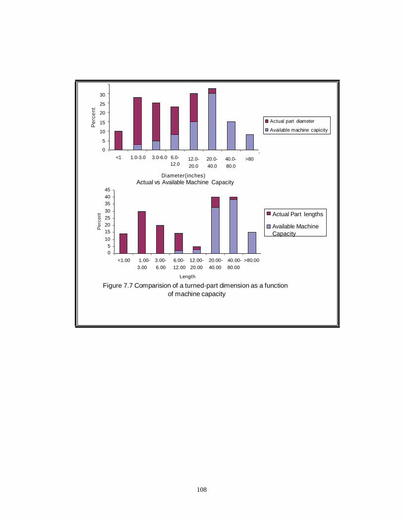
108

Pe

rce

nt

Perc

ent

30

25

20

15

10

5

0

<1 1.0-3.0 3.0-6.0 6.0-

12.0

12.0- 20.0- 40.0- >80

20.0 40.0 80.0

Actual part diameter

Available machine capicity

Diameter(inches)

Actual vs Available Machine Capacity

45

40

35

30

25

20

15

10

5

0

<1.00 1.00- 3.00- 6.00- 12.00- 20.00- 40.00- >80.00

3.00 6.00 12.00 20.00 40.00 80.00

Length

Actual Part lengths

Available Machine

Capacity

Figure 7.7 Comparision of a turned-part dimension as a function

of machine capacity

109

Pe

rce

nt

Pe

rce

nt

45

40

35

30

25

20

15

10

5

0

Maximum Speed(RPM)

Actual vs Available Machine Capacity

Actual Part

Speeds

Available

Machine

35

30

25

20

15

10

5

0

Maximum feed (Inch/Rev)

Actual Part

Speeds

Available

Machine

Figure 7.8 Comparision of maximum speeds and feeds

with maximum used

MODELS FOR MACHINE CELL AND PART FAMILY FORMATION One of the primary uses of coding system in manufacturing is to develop part families for

efficient workflow. Efficient workflow can result from grouping machines logically so that

material handling and setup can be minimized. The same tools and fixtures can be used by

grouping parts having similar operations. Due to this, a major reduction in setup results and also

material handling between machining operations is minimized.

Family formation is based on production parts or more specifically, their manufacturing feature.

Components requiring similar processing are grouped into the same family. There is no rigid rule

110

require similar routing. A user may want to put only those parts having exactly the same routing

sequence into a family. Minimum modification on the standard route is required for such family

members. Only, few parts will qualify for family membership. On the other hand, if one groups

all the parts requiring a common machine into family, large part families will results.

Before grouping can start, information related to the design and processing of all existing

components have to be collected from existing part and processing files. Each component is

represented in a coded form, called an operation-plan code (operation plan code, Table 7.8). An

OP code represents a series of operations on a machine and/or one workstation.

Operation code Operation plan

01 SAW 01 Cut to size 02 LATHE 02 Face end

Drill

Center drill

Ream

Bore

03

GRIND 05

Turn straight

Turn groove

Chamfer

Cutoff

Face

Grind

04 INSP 06 Inspect dimension

Inspect finish

1. operation-plan code (OP code) and operation plan

1 SAW 01 2 LATHE 02 3 GRIND 05

4 INSP 06 2. OP-code sequence

Table: Operation plan, OP code, and Op-code sequence

For example, we can use GRIND05 to represent the sequence; load the work piece onto the

grinding machine, attach the grinding wheel, grind the work piece, and unload the work piece

from the grinding machine. Operations represented by the Op code are called an operation plan.

It is not necessary that an OP code include all operations required on a machine for a component.

It is used to represent a logical group of operations on a machine, so that a process plan can be

represented in a much more concise manner. Such a representation is called an OP code

sequence. The main aim of an OP code is to simplify the representation of process plans. This

simplified process plan can be stored and retrieved

PRODUCTION FLOW ANALYSIS

problem for manufacturing cell design. This analysis uses the information contained on

production route sheets. Work parts with identical or similar routing are classified into part

111

families which can be used to form logical machine cells in a group technology layout. Since

PFA uses manufacturing data rather than design data to identify part families, it can overcome

two possible abnormalities that can occur in part classification and coding. First, parts whose

basic geometries are quite different may nevertheless require similar or identical process routing.

Second, parts whose geometries are quite similar may nevertheless require process routing that

are quite different.

The procedure in PFA consists of the following steps.

Machine classification. Classification of machines is based on the operation that can be

performed on them. A machine type is assigned to machines capable of performing

similar operations.

Checking part list and production route information. For each parts, information on the

operations to be taken and the machines required to perform each of these operations is

checked carefully

Factory flow analysis. This comprise a micro level examination of flow of components

through machines. Thus, it allows the problem to be decomposed into a number of

machine-component groups.

Machine-component group analysis. This analysis recommended manipulating the

matrix to form cells.

Many researchers have been subsequently developed algorithm to solve the family-formation

problem for manufacturing cell design. In PFA, a large matrix generally termed as incidence is

constructed. Each row represents an OP code, and each column represents a component. We can

define the matrix as Mij, where i indicates the optiz code and j indicates components for example

Mij = 1 if component j has OP code i; otherwise Mij = 0. The objective of PFA is to bring

together those components that need the similar set of OP codes in clusters.

Rank order clustering

This method is based on sorting the rows and columns of machine part incidence matrix. The

rank order clustering was developed by King (1980). Steps of this algorithm is given below

Step 1. For each row of the machine part incidence matrix, assign binary weight and calculate the

decimal equivalent

Step 2. Sort rows of the binary matrix in decreasing order of the corresponding decimal weights.

112

1 2 3 4 5

1 1 2

n k

n k

Step 3. Repeat the preceding two steps for each column.

Step 4. Repeat the preceding steps until the position of each element in each row and column

does not change.

A weight for each row i and column j are calculated as follows:

n

Row i : Wi = aik 2

k 1

m

Column j: Wj = akj 2

k 1

In the final matrix generated by the ROC algorithm, clusters are identified visually.

Example 7.3

Step 1. Assign binary equivalent to each row and calculate binary equivalent:

Part number

24 23 22 21 20 Part number 1 2 3 4 5 Decimal equivalent

1 1 1 11 1 1 20

1 1 10 Machine number

1 1 20

Step 2. Sorting the decimal weights in decreasing order results in the following matrix:

Part number

1 1 4

1 1 1 1

Machine number

1 1 3

Step 3. Repeating the proceeding steps for each column produces the following matrix:

Part number

1 3 2 4 5

1 1 2 1 1 4

1 1 1 1

1 1 3

Machine number

In this matrix two separate clusters are visible

Bond energy algorithm

McCormick, Schweitzer, and white (1972) developed an interchange-clustering algorithm called

the bond energy algorithm (BEA). The BEA seeks to form by minimizing the measure of

effectivene1ss. This is defined as follows:

ME= a a a m n a a ... (3)

2 i1 j1 ij i, j1 i , j1 i1, j i1, j

113

BEA algorithm

Step 1. Set j=1. Select one of the columns arbitrarily.

Step 2. Place each of the remaining n-j columns, one at a time, for each of j+1 positions, and

compute each column‘s contribution to the ME.

Place the column that gives the largest incremental contribution to the ME in its best location.

Increase j by 1 and repeat the preceding steps until j=n.

Step 3. When all the columns have been placed, repeat the procedure for the rows.

The BEA applied to the Example7.3 and is illustrated below in Example 7.4

Example 7.4

Step 1. Set j=1. Select column 2.

Step 2. Place each of the remaining columns in each of the j+1 position. The contribution to the

ME value of the column 2 is computed next:

Position

Column number

J=1 J+1 ME value

2 1 0

2 3 0

2 4 2

2 5 1

15 assemble these components into final product. Process planning acts as a bridge

Column 4 is placed in the j+1 position.

Machine number

15 assemble these components into final product. Process planning acts as a bridge

UNIT IV

COMPUTER AIDED PLANNING AND CONTROL, SHOP FLOOR CONTROL AND

INTRODUCTION TO FMS

1. Structure

Introduction

Objectives

Introduction to Process Planning

Approaches to Process Planning

Manual Experience-based Process Planning

Computer Aided Process Planning

Approaches to Computer Aided Process Planning (CAPP)

Variant Process Planning, Advantages and Disadvantages

Generative Process Planning, Advantages and Disadvantages

Knowledge-based Process Planning

Variant or Generative, Which to Use?

Feature Recognition in Computer Aided Process Planning

Approaches to Part Feature Recognition

Attributed Adjacency Graph Based Approach for Feature Recognition

An Illustrated Example

Recent Trends in Computer Aided Process Planning

Summary

Key Words

Answers to SAQs

INTRODUCTION

Before introduction to the role of computer aided process planning (CAPP), it is

worthwhile to understand the role of process planning in the product cycle. Once the

design of the product has been evolved from customer’s views, its manufacturing

necessitates careful planning and scheduling of the various processes of manufacture. So

that, the product is made to right specifications and delivered at the right time at a

minimal cost. The cycle from concept to design, planning, production, quality control

and feedback to design goes on in which one can easily understand the crucial role of

planning. In job/batch manufacture, as an enormous amount of data is needed for

planning as well as other activities, data bases are required and the flow of information

should be fast for a high performance of the total manufacturing system.

2. Objectives

After studying this unit, you should be able to

understand what is process planning and CAPP,

know the various steps involved in CAPP,

classify the various methods of CAPP, and

understand the feature recognition in CAPP.

INTRODUCTION TO PROCESS PLANNING

In manufacturing, the goal is to produce components that meet the design specifications.

15 assemble these components into final product. Process planning acts as a bridge

The design specification ensures the functionality aspect. Next step to follow is to

these operations are made. 16

Error!

CIM Modelling and

Operations between design and manufacturing by translating design specification into

manufacturing process detail. Hence, in general, process planning is a production

organization activity that transforms a product design into a set of instruction (sequence,

machine tool setup etc.) to manufacture machined part economically and competitively.

The information provided in design includes dimensional specification (geometric shape

and its feature) and technical specification (tolerance, surface finish etc.)

Now-a-days, process planning is applied to many manufacturing industries like metal

cutting, sheet metal forming, composite and ceramic fabrication and other manufacturing

processes. Figure 9.1 represents the various steps involved in developing a process plan.

Yes

No

Various steps are discussed as follows :

Figure 9.1

The analysis of finished part requirement is the first step in process planning. Initially

the features of parts are analyzed. Examples of geometric feature include plane, cylinder,

cone step, edge and include fillet. These common features can be modified by the

addition of slots, pockets, grooves, holes and others. The second step is the selection of

raw work piece shape, size (dimensions and weight), material and other attributes are

determined. Weight and material of the raw part are determined by the functional

requirement of plan.

The next logical step in process planning is to determine the appropriate types of

processing operations and their sequences to transform the features, dimensions and

tolerances of a part from the raw to the finished state. There may be many ways to

produce a design some times constraints are also considered like some feature be

machined before or after other. Furthermore, the types of machine, available tools as

well as batch size influence the process sequence.

Next step to be followed in process planning is the selection of machine tools on which

Implementation Selection of Tools, Work Holding Devices

(Fixtures) and Inspection Equipments

Process

Planner

Determining Machine Conditions (Cutting Speed, Feed, and Depth of Cut and Manufacturing Times (Processing

Time and LeadTime)

Analysis of Part Requirements

Design Specification

Selection of Machine Tools

Determining Manufacturing Operation and their Sequences

Selection of Raw Workpiece

Required Product

into inter-organizational flow. Main focus is to optimize the system performance in a 17

Some of the factors which influences the selection of machine tool are as follows :

(i) Attributes related to workpiece, such as desired features, dimensions of

workpiece, dimensional tolerances and raw material form.

(ii) Attributes related to machine tools, e.g. process capability size, mode of

operation, tooling capabilities and automatic tool changing capabilities.

(iii) Attribute related to production volume, e.g. production quantity and order

frequency.

Unit cost of production, manufacture lead time and quality are three basic criteria for

evaluating the suitability of a machine tool to accomplish an operation.

Next step to be followed is the selection of tools work holding devices and inspection

equipments. Features on the workpieces are generated using a combination of machine

tool and cutting tools. Work holding devices are used to locate and hold the workpiece to

generate features. In order to ensure the dimensional accuracy, tolerance and surface

finish on the feature, inspection equipments are required. Part features play a vital role in

the selection of machine tools, fixture and inspection equipment.

Now sixth step which has to be performed is the determination of machining condition

and manufacturing time. The controllable variables of machine condition are cutting

speed (υ), feed (f) and depth of cut (d).

Minimum cost per piece, maximum production rate and manufacture lead time are same

for the model to be optimized for high production and less cost.

APPROACHES TO PROCESS PLANNING

There are basically two approaches to process planning which are as follows :

(i) Manual experience-based process planning, and

(ii) Computer-aided process planning method.

Manual Experience-based Process Planning

The steps mentioned in the previous section are essentially same for manual process

planning. Following difficulties are associated with manual experienced based process

planning method :

It is time consuming and over a period of time, plan developed are not

consistent.

Feasibility of process planning is dependent on many upstream factors

(design and availability of machine tools). Downstream manufacturing

activities such as scheduling and machine tool allocation are also influenced

by such process plan.

Therefore, in order to generate a proper process plan, the process planner must have

sufficient knowledge and experience. Hence, it is very difficult to develop the skill of the

successful process planner and also a time consuming issue.

Computer-Aided Process Planning

Computer-aided process planning (CAPP) helps determine the processing steps required

to make a part after CAP has been used to define what is to be made. CAPP programs

develop a process plan or route sheet by following either a variant or a generative

approach. The variant approach uses a file of standard process plans to retrieve the best

plan in the file after reviewing the design. The plan can then be revised manually if it is

not totally appropriate. The generative approach to CAPP starts with the product design

specifications and can generate a detailed process plan complete with machine settings.

CAPP systems use design algorithms, a file of machine characteristics, and decision

logic to build the plans. Expert systems are based on decision rules and have been used

in some generative CAPP systems.

CAPP has recently emerged as the most critical link to integrated CAD/CAM system

Computer Aided

Process Planning

necessary and vital objective of CIM system. 18

CIM Modelling and

Operations global context. The essentiality of computer can easily be understood by taking an

example, e.g. if we change the design, we must be able to fall back on a module of CAPP

to generate cost estimates for these design changes. Similarly for the case of the

breakdown of machines on shop floor. In this case, alternative process plan must be in

hand so that the most economical solution for the situation can be adopted. Figure 9.2 is

one such representation, where setting of multitude of interaction among various

functions of an organization and dynamic changes that takes place in these sub

functional areas have been shown. Hence, the use of computer in process planning is

essential.

Figure 9.2 : Framework for Computer Aided Process Planning

CAPP is the application of computer to assist the human process planer in the process

planning function. In its lowest form it will reduce the time and effort required to prepare

process plans and provide more consistent process plan. In its most advanced state, it

will provide the automated interface between CAD and CAM and in the process achieve

the complete integration with in CAD/CAM.

1. Advantages Over Manual Experience-based Process Planning

The uses of computers in process plan have following advantages over manual

experience-based process planning :

(i) It can systematically produce accurate and consistent process plans.

(ii) It leads to the reduction of cost and lead times of process plan.

(iii) Skill requirement of process planer are reduced to develop feasible process

plan.

(iv) Interfacing of software for cost, manufacturing lead time estimation, and

work standards can easily be done.

(v) Leads to the increased productivity of process planar.

With the emergence of CIM as predominate thrust area in discrete part industries

process planning has received significant attention, because it is the link between

CAD and CAM. Hence, computer aided process planning (CAPP) has become a

Product Design and Development Request

Part List Connected data

Geometry Data

Parts Master Files

Process Plans

Production Order

Actual Data

Machine, Tool, Fixture Data Bands NC Corrected

Program Data

Production Control CAM

CAPP

CAD

Organizational Planning System

MRP Material Resource

Planning Capacity Planning

19

Header Data

Formatting

Part Family

Search

Process Plan Formatting

Work Element

Processing

Part Family Matrix File

Part Classification Code

Computer Aided

Process Planning

Header Data Formatter

Header Data Input

Standard Sequence File

Editing

Information

Operation Plan File

Editing Information

Process Plan

Application Program

Work Element Processor

Process Plan

Formatter

Process Plan

Figure 9.3 : Flow Diagram of the CAPP Process Planning System

2. Steps Involved in CAPP

Now-a-days, rapid progress is being made in the automation of actual production

process and also the product design element. However, the interface between

design and production presents the greatest difficulty in accomplishing integration.

CAPP has the potential to achieve this integration. In general, a complete CAPP

system has following steps :

(i) Design input

(ii) Material selection

(iii) Process selection

(iv) Process sequencing

(v) Machine and tool selection

(vi) Intermediate surface determination

(vii) Fixture selection

(viii) Machining parameter selection

(ix) Cost/time estimation

(x) Plan preparation

(xi) Mc tape image generation.

Operation Plan

Retrieve/Edit

Standard Sequence

Retrieve/Edit

20

CIM Modelling and

Operations

APPROACHES TO COMPUTER-AIDED PROCESS PLANNING

In recent days, several computer-aided process planning systems are available for use for

a variety of manufacturing operation.

These systems can broadly be clarified into two categories :

(i) Variant computer aided process planning method.

(ii) Generative computer aided process planning method.

The details of these are explained in next subsections.

Variant Process Planning, Advantages and Disadvantages

Variant process planning approach is sometimes referred as a data retrieval method. In

this approach, process plan for a new part is generated by recalling, identifying and

retrieving an existing plan for a similar part and making necessary modifications for new

part. As name suggests a set of standard plans is established and maintained for each part

family in a preparatory stage. Such parts are called master part. The similarity in design

attributes and manufacturing methods are exploited for the purpose of formation of part

families. Using coding and classification schemes of group technology (GT), a number

of methods such as coefficient based algorithm and mathematical programming models

have been developed for part family formation and plan retrieval. After identifying a new

part with a family, the task of developing process plan is simple. It involves retrieving

and modifying the process plan of master part of the family.

The general steps for data retrieval modification are as follows :

3. Establishing the Coding Scheme

A variant system usually begins with building a classification and coding scheme.

Because, classification and coding provide a relatively easy way to identify

similarity among existing and new parts. Today, several classification and coding

systems are commercially available. In some extreme cases, a new coding scheme

may be developed. If variant CAPP is preferred than it is useful for a company to

look into several commercially available coding and classification systems (e.g.

DCLASS, JD-CAPP etc.). Now, it is compared with companies before developing

their own coding and classification system. Because using an existing system can

save tremendous development time and manpower.

(i) Form the Part Families by Grouping Parts

The whole idea of GT lies into group numerous parts into a manageable

number of part families. One of the key issues in forming part families is

that all parts in the same family should have common and easily identifiable

machined features. As a standard process plan are attached with each part

family, thereby reducing the total number of standard process plans.

(ii) Develop Standard Process Plans

After formation of part families, standard process plan is developed for each

part families based on common part features. The standard plan should be

as simple as possible but detailed enough to distinguish it from other.

(iii) Retrieve and Modify the Standard Plans for New Parts

Step1 to step 3 are often referred as preparatory work. Each time when a

new part enters the systems, it is designed and coded based on its feature,

using the coding and classification scheme, and than assigned to a part

family. The part should be similar to its fellow parts in the same family.

Also, family’s standard plan should represent the basic set of processes that

the part has to go through. In order to generate detailed process routes and

20

operation sheets to this part, the standard plan is retrieved from the data

21

Material Requirement File

Machine Sequence File

Machine Tool File

Tool Fixture File

Mfg. Times File

Labour Cost File

Text Generator

Activity Text Generation

base and modified. Modification is done by human process planar. After

this stage parts are ready for release to the shop.

The success of aforementioned process planning system is dependent on

selection of coding scheme, the standard process plan and the modification

process, because the system is generally application oriented. It may be

possible that one coding scheme is preferable for one company and same is

not for other company.

Due to use and advancement of computers, the information management

capability of variant process planning is much superior. Otherwise it is quite

similar to manual experience-based planning.

4. Advantages and Disadvantages of Variant CAPP

Following advantages are associated with variant process planning approach:

(i) Processing and evaluation of complicated activities and managerial issues

are done in an efficient manner. Hence lead to the reduction of time and

labour requirement.

(ii) Structuring manufacturing knowledge of the process plans to company’s

needs through standardized procedures.

(iii) Reduced development and hardware cost and shorter development time.

This is an essential issue for small and medium scale companies, where

product variety is not so high and process planner are interested in

establishing their own process planning research activities.

5. Disadvantages of Variant Process Planning Approach

Following disadvantages are associated with variant process planning approach

(i) It is difficult to maintain consistency during editing.

(ii) Proper accommodation of various combinations of attributes such as

material, geometry, size, precision, quality, alternate processing sequence

and machine loading among many other factors are difficult.

(iii) The quality of the final process plan largely depends on the knowledge and

experience of process planner. The dependency on process planner is one of

the major shortcomings of variant process planning.

Master Variant File

Process Variant File

Process Selection Logic

Computer Aided

Process Planning

Finished Part

Description

Bill of Materials

Part No.

Process Deviation

Process Plan

Activity Report

Activity

Variant Process

Planning

21

Figure 9.4 : Framework of Variant Process Planning Activity

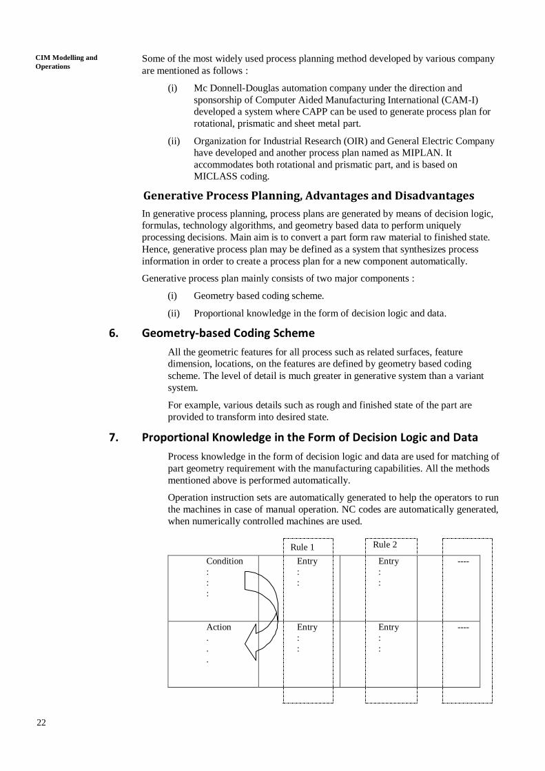
22

CIM Modelling and

Operations Some of the most widely used process planning method developed by various company

are mentioned as follows :

(i) Mc Donnell-Douglas automation company under the direction and

sponsorship of Computer Aided Manufacturing International (CAM-I)

developed a system where CAPP can be used to generate process plan for

rotational, prismatic and sheet metal part.

(ii) Organization for Industrial Research (OIR) and General Electric Company

have developed and another process plan named as MIPLAN. It

accommodates both rotational and prismatic part, and is based on

MICLASS coding.

Generative Process Planning, Advantages and Disadvantages

In generative process planning, process plans are generated by means of decision logic,

formulas, technology algorithms, and geometry based data to perform uniquely

processing decisions. Main aim is to convert a part form raw material to finished state.

Hence, generative process plan may be defined as a system that synthesizes process

information in order to create a process plan for a new component automatically.

Generative process plan mainly consists of two major components :

(i) Geometry based coding scheme.

(ii) Proportional knowledge in the form of decision logic and data.

6. Geometry-based Coding Scheme

All the geometric features for all process such as related surfaces, feature

dimension, locations, on the features are defined by geometry based coding

scheme. The level of detail is much greater in generative system than a variant

system.

For example, various details such as rough and finished state of the part are

provided to transform into desired state.

7. Proportional Knowledge in the Form of Decision Logic and Data

Process knowledge in the form of decision logic and data are used for matching of

part geometry requirement with the manufacturing capabilities. All the methods

mentioned above is performed automatically.

Operation instruction sets are automatically generated to help the operators to run

the machines in case of manual operation. NC codes are automatically generated,

when numerically controlled machines are used.

Rule 1 Rule 2

Condition

:

:

:

Entry

:

:

Entry

:

:

----

Action

.

.

.

Entry

:

:

Entry

:

:

----

22

F

i

g

u

r

e

9

.

5

:

F

r

a

m

e

w

o

r

k

o

f

a

D

e

c

i

s

i

o

n

T

a

b

l

e

23

Manufacturing knowledge plays a vital role in process planning. The process of

acquisition and documentation of manufacturing knowledge is a recurring

dynamic phenomenon. In addition, there are various sources of manufacturing

knowledge such experience of manufacturing personnel, handbooks, supplier of

machine tools, tools, jigs and fixtures materials, inspection equipment and

customers etc. Hence, in order to understand manufacturing information, ensuring

its clarity and providing a framework for future modification, it is not only

necessary but also inevitable to develop a good knowledge structure from wide

spectrum of knowledge. Flowchart, decision trees, decision tables, algorithms,

concepts of unit machined surfaces, pattern recognition techniques, and artificial

intelligent based tools are used to serve the purpose. A brief discussion on

decision table is given below.

The basic elements of decision tables are condition, action and rules. They are

represented in the form of allocation matrix. Figure 9.4 is one such representation

where condition states the goal that we want to achieve and action states the

operation that we have to perform. On the basis of experience the expert rules are

formed by entry values to establish the relationship between condition and action.

Table 9.1 is one such representation where entry are of Boolean-types (true, false,

don’t care). Similarly, in Table 9.2, continuous value type entries are shown.

8. Table 9.1 : Boolean Value-Type Entries

Length of bar 8 in. T* F

Diameter of bar 1 in.

Diameter of bar 1 in. T T

- - - -

Extra Support T

* T : True; F : False; blank : don’t care.

9. Table 9.2 : Continuous Value-type Entries

Length of bar (in) 4 4 16 16

Diameter of bar (in.) 0.2 > 0.2 1>diameter>0.2 1

Extra support T T T

* T : true; blank : do not care

The decision making process works as follow.

For a particular set of condition entries, look for its corresponding rule from that rule

determine the action.

10. Advantages of Generative Process Plan

Generative process plans have a number of advantages. Among the major ones are

the following :

(i) They rely less on group technology code numbers since the process, usually

uses decision tree to categorize parts into families.

(ii) Maintenance and updating of stored process plans are largely unnecessary.

Since, any plan may be quickly regenerated by processing through the tree.

I

n

d

e

e

d

,

m

a

n

y

a

r

g

u

e

t

h

a

t

w

i

t

h

g

e

n

e

r

a

b

l

e

s

y

s

t

e

m

s

,

p

r

o

c

e

s

s

p

23

lans should not be stored since if the process is changed, and out-of-dated

process plan might find its way back into the system. Computer Aided

Process Planning

24

CIM Modelling and

Operations (iii) The process logic rules however must be maintained up to dated and ready

for use. This provides the process planner with an assurance that the

processes generated will reflect state-of-the-art technology.

Description of various generative and variant and generative CAPP systems is

mentioned Table 9.3.

11. Table 9.3 : Some of the Variant and Generative CAPP Systems

CAPP

System

Part

Shapes

Process

Planning

Approaches

Characteristics and

Commercial

Situation

Programming

Languages

Used

Developers

CMPP Rotational Generative Uses English like

language(COPPL)

FORTRAN 77 UTRC (USA)

GENPLAN All Variant and

Generative

Interfaced with

CAD\CAM Lockheed-

Georgia(USA)

GT-CAPP All Generative Part family code

used Rockwell Inc

(USA)

KAPPS Rotational

and

Prismatic

Generative Part family numbers

used

LISP Kobe Univ.

(JAPAN)

MIPLAN Rotational

and

Prismatic

Variant Expert system based

on MICLASS OIR and GE

Co.(USA)

RTCAPP Prismatic Generative Generic shell USC (USA)

TURBO- CAPP

Rotational Generative Knowledge based interfaced with CAD

PROLOG Penn. State Univ (USA)

XPLAN All Generative Expert system based

on DCLASS

FORTRAN 77 Tech. Univ. of

DK (Denmark)

XPLAN-R Rotational Generative Expert system based

on DCLASS

FORTRAN 77 Tech. Univ. of

DK (Denmark)

XPLANE Rotational Generative Knowledge based FORTRAN Twente Univ.

Tech.

(Netherland)

XPS-1 All Variant and

Generative

COPPL used FORTRAN UTRC and

CAM-I (USA)

(Source : Alting and Jhang (1989))

Knowledge-based Process Planning

The main forces behind to apply knowledge-based (KB) techniques for CAPP is the

requirement of large amount of human expertise in CAPP. Based on the previous

discussion, one realizes that a productive CAPP system must contain tremendous amount

of knowledge – facts about the machine and shop environment as well as rules about

sequencing machining operations must be included. A traditional CAPP program cannot

learn new knowledge without a programmer explicitly rewriting it. The rigidity of

traditional methodology endangers the implementation of CAPP systems. A KB system

stores knowledge in a special manner so that it is possible to add, delete and modify facts

and rules in the knowledge base without rewriting the program, i.e. it learns new things

according to embedded learning procedures.

A complete set of manufacturing knowledge is not equipped by any existing

knowledge-based process planning system. Most of these systems focus on a small

portion of the issues in the domain of automated process planning using an expert

systems approach. Some of them are :

12. EXCAP Family of Process Planning Systems

EXCAP, EXpert Computer-Aided Process Planning, developed by Davies and

24

Darbys

hire, is

a

knowle

dge-

based

system

for

rotation

al part

process

plannin

g.

25

EXCAP-A and EXCAP-Y are previous generations of the current member of the

EXCAP family of process planning systems.

13. GARI

GARI is the first AI-based CAPP program to appear in the literature. It is

implemented in MACLISP and operates on CII-Honeywell Bull HB-68 computer

under the MULTICS operating system. GARI utilizes production rules in its

knowledge representation and generates a process plan from a model of the part. It

emphasizes the “conflict resolution”. The knowledge is rather subjective and

specialized. As a result, in the planning process, “compromises are often

necessary.”

14. TOM : Technostructure of Manufacturing

TOM is another production rule-based CAPP system written in PASCAL and runs

on VAX computer. TOM was designed to accept input in two ways: (1) directly

entering part desecration by the user, and (2) translating design data from

COMPAC CAD system. TOM can deal with “holes” exclusively.

15. SIPP : Semi-Intelligent Process Planner

SIPP is an AI-based CAPP system for the creation of metal parts using chip metal

removal operations. It is written in PROLOG and utilizes “frames” as its

knowledge representation scheme instead of using production rules. Frames are

used to represent two types of knowledge: (1) information about the

characteristics of various kinds of machinable surfaces, and (2) the capabilities of

various machining processes.

Computer Aided

Process Planning

16. SIPS

SIPS, another AI-based CAPP system which selects machining operations for the

creation of metal parts, is a successor to SIPP. It is written in LISP and is currently

being integrated into the AMRF (Automated Manufacturing Research Facility)

project, where it is used to select machining operations on a feature by feature

basis.

Like SIPP, SIPS also employs branch and bound search strategy for the least-cost-

first solution in its inference engine. The basic difference between SIPP and SIPS

is that SIPS used a new knowledge representation technique, called hierarchical

knowledge clustering, instead of “flat” frames to represent problem-solving

knowledge.

17. TOLTEC

TOLTEC is a system equipped with some learning capability. It takes input as

feature-based part description interactively. The features are represented in a

frame structure. It generates output in a form of operations and their sequence.

18. Turbo-CAPP

Turbo-CAPP is a knowledge-based CAPP system written in PROLOG and capable

of :

extracting and interpreting surface features from a 2&1/2-D CAD data base.

performing intelligent reason for process planning.

learning new process and machining capabilities.

generating alternative process plans (based on the current status of the

knowledge base).

creating generic NC part programs for automated.

25

Turbo-CAPP is designed to handle strictly symmetric rotational parts. It employs a

backward chining inference mechanism for plan generation. In the process of

26

CIM Modelling and

Operations creating process plan and NC codes, the system must acquire knowledge from the

user from time to time.

19. XPS-2 Family of CAPP Systems

CAM-I started the first structured development of process planning systems. It

then embarked on a form-feature based, generative planning project, XPS and

accomplished with the completion of XPS-2 in 1987. The form feature used to

implement XPS-2 were taken from a “feature taxonomy” developed by CAM-I.

20. Other Knowledge-Based CAPP Systems

Rather than aforementioned Knowledge-Based CAPP System some other KB

process planning systems are in existence :

(i) CMPP (Austin, 1996) is a planning system for planning cylindrical parts

(also for some non-cylindrical features). It performs dimension, tolerance,

and stock removal analysis based on a sophisticated algorithm with the

objective of optimizing tolerance capabilities of shop equipment.

(ii) Hi-MAPP developed by Brenfi and Khoshnevis.

(iii) Wolfe and Kung in 1984 developed a CAPP system, which reads part

geometry from a PADL model and generates process plans automatically.

Variant or Generative, Which to Use?

What CAPP approach (Variant or Generative) is better? This question has been

constantly asked but, there is no definite answer to it.

Generally speaking, a variant system is better for manufacturing setting where similar

parts are manufactured repetitively. Because parts are similar, Group Technology can

easily be implemented and shows quick and significant return on investment (ROI).

Because similar parts are produced repetitively, process plan can be retrieved, slightly

modified and used, without going through too much trouble. On the other hand,

generative process planning is better suited for a manufacturing environment in which

part does not exhibit too much similarity and new part are introduced on a regular basis.

In this case, benefits cannot be gained from Group Technology due to dissimilarity of

parts. Because, new parts are regularly introduced, historical data does not have too

much value to the process planner. However, aforementioned approach is a rough

guideline for selecting the appropriate CAPP approach.

3. SAQ 1

(a) What is process planning?

(b) What are the various steps in developing a process plan?

(c) Why the need for CAPP arises?

(d) What are different approaches to CAPP? Describe briefly.

(e) Briefly describe the “Knowledge based Process Planning”.

(f) Write short notes on following :

(i) Manual experience based process plan.

(ii) Computer Aided Process Plan.

well. This approach is encouraging because, conceptually, it can be applied for more 27

FEATURE RECOGNITION IN CAPP Computer Aided

Process Planning

As we have seen that CAPP system usually serve as link in integrating the CAD and

CAM. However, it is only the partial link due to lack of part feature information

provided by existing CAD/ Drafting system. Part feature information is an essential data

for CAPP. In other words, it is a tedious job for CAPP to understand the three

dimensional geometry of the designed part from CAD system in terms of their

engineering meaning related to assembly and manufacturing. Generally, all CAPP

planning method and systems suffered from such type of problem and is referred as

feature recognition in CAPP.

Hence, objective of feature recognition is to bridge the gap between the database and

automated process planning systems by automatically distinguishing the feature of a part

from the geometry and topological data stored in the CAD system. The essence of

feature recognition can easily be understood by taking an example as shown in

Figure 9.6. This figure is defined by a constructive solid geometry tree that represents a

block primitive and a cylinder primitive combined by the Boolean operator “-”. Shape

and dimension can easily be identified by these schemes but, some higher level

information is not provided by this scheme such as, whether the hole is blind hole or

through hole. Such types of information are called as feature. Hence, features play a vital

role in CAPP. In order to identify features and to solve CAD / CAPP interface problem,

feature recognition is one of the most efficient technique.

Feature recognition transforms a general CAD model into an application specific feature

model. In general, a generic part feature recognition system must be able to resolve

following issues.

(i) Extract design information of a part.

(ii) Identify all surfaces of part.

(iii) Recognize reasons about\and\or interpret these surfaces in terms of Part

features.

Once the features are classified, the automated planning system could develop the

required process plan to make the part and hence, eliminate the need for a human to

translate the CAD data into something that process planning system can understand.

Here, it is pertinent to mention that feature recognition is not only applicable to CAPP

system but it can also be applied to various other engineering applications that require

information about feature of parts classification and automated coding in GT.

Is a blind hole or through hole?

Figure 9.6 : Advance Level Information

Approaches to Part Feature Recognition

The most robust description of any part is provided through solid modelling. Therefore,

these appear to be a logical starting point for developing a feature recognition system.

Henderson and Anderson developed a system called FEATURES to perform automatic

feature recognition using data from solid modelling system. A FEATURE simulates the

human interpretation of part features. The system consists of a feature recognizer,

extractor, and organizer. For objects containing swept features, this system performs

28

CIM Modelling and

Operations complex parts. The FEATURES system uses the boundary representation (BREP) of a

part, which denotes the faces, edges and vertices (FEV). Thus, features such as holes

must be derived from more primitive data.

1. Table 9.4 : A Brief Review and Recent Trends in Feature Recognition Research

Author Part Feature-recognition System Recognizable

Features

CAM-1 From feature taxonomy --

Choi CAD/CAM-compatible, toll-oriented process

planning system.

Holes, Slots,

Pockets

Henderson

and Anderson

Extraction of feature information from 3-D CAD data. Holes, Slots,

Pockets

Jalubowski Syntactic characterization of machine part shapes. Rotational part

family

Kakazu and

Okino

Pattern-recognition approaches to GT code

generation.

Rotational GT

code

Kakino et.al. A method of parts description for computer-aided

production planning.

Grooves,

steps, flanges

Kung Feature-recognition and expert process planning

system

Holes, Slots,

Pockets

Kyprianou Shape features in geometric modelling Rotational part

family

Lee Integration of solid modelling and data base

management for CAD/CAM

--

Liu Generative process planning using syntactic pattern

recognition.

--

Srinrasan, Liu

and Fu

Extraction on manufacturing details from geometric

models

Rotational part

family

Woo Computer-aided recognition of volumetric designs --

Representing FEV contained in a BREP graph. As a result a hole may be present as a

collection of faces that must be recognized from the part data.

A number of approaches to part feature recognition for rotational as well as prismatic

parts have been developed. These different approaches are enlisted as follows :

(i) Syntactic Pattern Recognition

(ii) State Transition Diagram and Automata

(iii) Geometry Decomposition Approach

(iv) Expert System Rule Logic

(v) CSG (Set Theoretic) Approach

(vi) Graph Based Approaches

The syntactic pattern recognition and/or expert logic approach are mainly applied for

feature extraction of rotational part feature recognition. The complexity increases in case

for prismatic parts due to lack of rotational property. In this case, the difficulty of both

representation of a generic object and recognition of its feature increases extensively. A

brief review and recent trends in feature recognition research has been enumerated in

Table 9.4.

In next subsection, we have discussed the graph based approach to feature recognition.

F1 is adjacent to F2 and F4 29

:

Attributed Adjacency Graph Based Approach for Feature Recognition

Following three steps are involved in Graph based feature recognition

(i) Generating graph based representation of the object to be recognized.

(ii) Defining part features.

(iii) Matching part features in the graph representation.

2. Generating Graph Based Representation of the Object to be Recognized

During first step graphs are used for representation of the object. This step is

necessary because data extracted from the data base are usually in the form of

boundary representation (BREP) and can not be used for feature recognition.

Information regarding the type of face adjacency and relationship between the sets

of faces should be expressed explicitly to recognize a feature. Here, attribute

adjacency graph (AAG) has been used to demonstrate the recognition process.

Attributed Adjacency Graph

An AAG can be defined as a graph G = (N, A, T), where N is the set of

nodes, A is the set of arcs, T is the set of attributes to arcs in A such that :

For every face f in F, there exists a unique node n in N.

For every edge e in E, there exists a unique arc a in A, connecting

nodes ni and nj, corresponding to face fi and face fj, which share the

common edge e.

“t” is an attribute assigned to every arc a in A, where :

t = 0 if the faces sharing the edge form a concave angle ( or “ inside”

edge)

t = 1 if the faces haring the edge form a convex angle (or “outside”

edge).

The AAG is represented in the form of matrix as follows :

Computer Aided

Process Planning

F1

F1 E1,1

F2

E1,2

...

E1,3

...

...

Fn

E1,n

F2 : : : : :

:

:

: :

: : :

: : : :

Fn

En,1 En,2 ... ... En,n

where 0 if Fi forms a concave angle with Fj

Eij = 1 if Fi forms a convex angle with Fj

if Fi is not adjacent to Fj

Hence it can easily be understood from above observation that AAG defines

the shape of a part uniquely up to its topology, if and only if the faces are

cut orthogonally.

3. Definition of Part Feature

First we have to define what actually feature is? In general any shape can be

feature if their manufacturing meanings are defined. There are mainly six features

which are commonly used in manufacturing. These are step, slot, three side

pocket, four side pocket, pocket (or blind hole) and through hole. Figures 9.7(a-f)

F1 is adjacent to F2 and F4 29

represent some of the features and their surfaces are labeled.

Four-side Pocket

30

CIM Modelling and

Operations

(a)

(b)

F3 is adjacent to F2 and F4

F2 is adjacent to F1, F3, and F4

F4 is adjacent to F1, F3 and F2

F1 forms concave (90o) angles with F2 and F4

F2 forms concave (90o) angles with F3, F1 and F4

F3 forms concave (90o) angles with F2 and F4

F4 forms concave (90o) angles with F1, F2 and F3

Blind Hole (Pocket)

F1 is adjacent to F2, F4 and F5

F2 is adjacent to F1, F3 and F5

F3 is adjacent to F2, F4, and F5

F4 is adjacent to F1, F3, and F5

F5 is adjacent to all other surfaces of the pocket

F1 forms concave (90o) angles with F2, F4 and F5

F2 forms concave (90o) angles with F3, F1 and F5

F3 forms concave (90o) angles with F2 and F4 and F5

F4 forms concave (90o) angles F3, F1 and F5

F5 forms concave angle (90o) with all other surfaces of the pocket

(c)

F1

F2

0 F F

F3

F1 F1

0 F

0

2 F3

F2

F1

0

0

F3

F2

0

F2

F3

F1

31

(d) Computer Aided

Process Planning

(e) F3

F1

F4

F2

4. M

atching the Features

Figure 9.7(a-f) : Various Features

After execution of step 1 and 2, the main task is to recognize AAG subgraph

(f) F3

F2 F1

F4

F1 0 F2

0 0

F4 0 F3

F2 F1

F4

F3

F2

0 0

F1 0 F3

0 F4

0

F1 0

0 F2

0 0 F5

0

0 0

F4 F3

0

31

instead of recognizing machining features in parts. Because, complete AAG graph

represents the part and subgraphs represent the features. It is computationally

complex task to identify subgraphs in a graph. Although, there is no general way

or algorithm to solve the problem.

Joshi and Chang, 1988 used an algorithm to identify the components of the graph

that could form a feature. The algorithm is based on the following observations :

A face that is adjacent to all its neighbouring faces with a convex angle 270o does

not form part of a feature. This observation is used as a basis for separating the

original graph into subgraphs that could corresponds to features. The separation is

done by deleting some nodes of the graph. The delete node rule follow IF THEN

rule and given as follows. For all nodes :

If (all incident arcs of a node have attribute “1”)

Then (delete this node (and all the incident arcs at the node) from AAG)

Delete node rule actually delete rows and column that represent the nodes in the

matrix. Now feature recognition rule are applied to identify that whether or not a

sub-graph represent a feature. On the basis of feature definition some rules are

written. In order to identify features some rules are given as follows :

For a Given AAG

It is a four side feature if

(The AAG subgraph has four nodes) and (The number of arcs with

attribute “0” is the number of nodes plus one).

It is a pocket feature if

(The AAG subgraphs have five nodes) and (The number of arcs with

attribute”0” is the number of attributes plus three).

32

.

.

.

CIM Modelling and

Operations In some of the cases, delete node rule fails. This is due to the intersection of

features. Delete node rule cannot separate complete AAG graph into subgraphs,

particularly for the case when features intersects. Hence, only for those cases

when features are disjoint, delete node rule can be applied.

Following procedures are used to separate the subgraphs for intersecting features.

Delete all 1 arcs

Form the subgraphs that may or may not represent the features.

If not all the subgraphs, represent features, restore the one arc deleted

within the subgraph.

The main task of this procedure is to separate the graphs into subgraphs. If the

procedure is successful, it greatly reduces the computational effort otherwise

graph remains unchanged.

An Illustrative Example An example is taken from Li (1992), which is illustrated as follows

5. Example 9.1 It is easy for human to recognize that the part shown in Figure 5.14(a) has a slot

and a pocket feature. In this example, however, we simulate the computer to apply

the feature recognition algorithm discussed earlier. We, therefore, want to solve

the following problem :

(i) Develop the AAG of the object, (ii) Give the matrix representation of the

AAG, and (iii) Recognize the features in this object.

6. Solution (i) First, we have to label each surface of the part. Given that the part is labeled

as shown in Figure 9.8(a), we develop the AAG as shown in

Figure 9.8(b) from the definition of AAG. By the definition of AAG we

mean that each surface of this part is represented by a node and each edge

by an arc with attribute 1 or 0.

(ii) For propose of inputting the AAG graph into the computer, we have to

convert the graph to matrix form. The matrix representation of AAG is

given as follows.

F1 F1 F2 F3 F4 F5 F6 F7 F8 F9 F10 F11 F12 F13 F14 F1 5

F2 F3

F4

F5 F6

F7

F8 F9

F10

F11

F12

F13

F1

4

F1

5

2. 9 0 9 . 9 0

. .

. . . . . . . . .

. .

. . . s y m . . .

. .

. . . 0 0 1 9 9 0 1 9 0 0 1 9 9 9 1 9 . 9 9 9 . . 9 1 . . . 9 . . . . . . . . . . . .

m e t r . . . .

. . . .

. . . .

. . . .

.

.

.

.

.

.

9

.

.

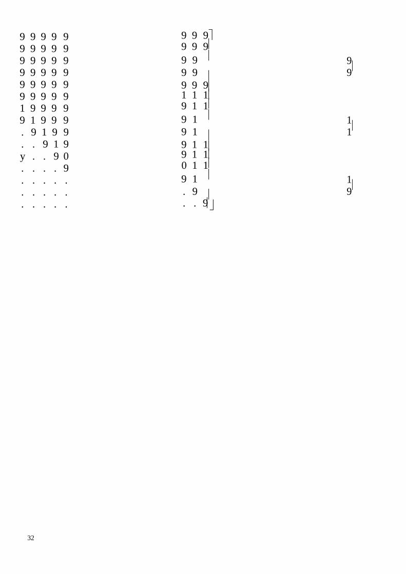
32

9 9

1 1

9 1

9 9 9 9 9 9 9 9 9 9 9 9 9 9 9 9 9 9 9 9 9 9 9 9 9 9 9 9 9 9 1 9 9 9 9 9 1 9 9 9 . 9 1 9 9 . . 9 1 9

y . . 9 0 . . . . 9 . . . . . . . . . . . . . . .

9 9 99 9 9

9 9

9 9

9 9 91 1 19 1 1

9 1

9 1

9 1 19 1 10 1 1

9 1

. 9

. . 9

33

(iii) Apply the delete node rule of the algorithm; that is delete the nodes

connected with all “1” attributer arcs. Also delete these “1” arcs. Doing this

on the adjacent matrix, we remove the rows and columns without

0 elements. For example, row 15 and column 15 represent this type of arc

and can be deleted. After all such arcs are deleted, the present matrix will

result into two unrelated sub-matrices. Each sub-matrix represents a sub-

graph. We find that “0” in column 12, which is F12. We find that two disjoint

subgraphs are generated (from Figure 9.8(d)). Figure 9.8(c) gives the same

structure as the one shown in Figure 9.8(b), which corresponds to the slot

feature. Thus the first feature that is recognized is the slot feature. In the

computer this matching is achieved by applying the identifying rules. That

is, if AAG subgroup has three nodes and the number of arcs with attribute

“0” is 2, and then it is a slot. Also, because Figure 9.8(d) has the same

structure as the one shown is Figure 9.7(e), it is a pocket. As there are no

more features to be recognized. We conclude that there are two features in

this part, a slot and a pocket.

Computer Aided

Process Planning

Figure 9.8(a)

Figure 9.8(b) : AAG for the Example Part

(c) AAG for Slot Features

0 1 0

0

0 4

0 1

2 3 1

1 7 1 8

1

1

9

1 1

0 1 0 0

1 1 1 1

1 1

1 5

6 10

1

1 1 1

14

1 1 1

13 0

1

12

0

1 15

1 11

15 3

9 10

11 2

12 1 5 6

13 7

4

8

14

4 0 1

0 0

0 5 0

0 0

3 2 0

34

CIM Modelling and

Operations

Figure (d) : AAG for Pocket Feature

RECENT TRENDS IN CAPP

In the global competitive market, various areas such as design process planning,

manufacturing and inspection plays a vital role in reducing cost and lead time. In the

various areas, different kind of interference mechanism has been developed. A lot of

difficulty arises while integrating the goal in CIM environment. For example, all

functional areas have its own standalone relational database and associated database

management system. One of the main difficulties posed in CIM environment is the

incompatibility of software and hardware incompatibility. Hence, it is not only desirable

but also inevitable to develop a single database technology to address these problems.

The major challenges of and research areas are to make CAPP system affordable to the

medium and small scale manufacturing industries. Hence recent trends in CAPP systems

include :

Automated translation of the design dimensions.

Tolerances into manufacturing dimensions.

Tolerances considering process capabilities.

Dimensional chains.

And to make CAPP system affordable for small and medium scale

manufacturing industries.

1. SAQ 2

(a) What do you mean by Feature Recognition?

(b) What are different steps of Graph based approach?

(c) Mathematically define AAG.

(d) Discuss about future trends in CAPP.

(e) What are the achievements of CIM?

SUMMARY

In the early 1970s, the function of process planning received very little attention. Today,

manufacturing environment has become more complex and competition has become

more intense. Hence, process planning has been accepted as critical to the success of

many companies. Process planning bridges the gap between design and manufacturing.

In addition, it has been acknowledged to be the link between CAD and CAM. As a result

process planning is recognized as a vital element in CIM environment.

This unit dealt with process planning where more focus was concentrated on CAPP. It

begins with the introduction of process planning and its various components. We

discussed and illustrated with examples the element of process planning, such as analysis

11 0 12 0 13

of part requirement; selection of the raw workpiece; determining manufacturing

operation and their sequences; selection of machine tools; selection of tools, jigs or

fixtures and inspection equipment; and determining machining condition and

manufacturing times (setup time, processing time and lead time). After that Computer

Aided Process Planning is discussed by explaining the reason why Computer Aided

Process Planning has recently received much attention both in industry and academia. It

follows by an overview of basic approaches for building Computer Aided Process

Planning system : variant and generative. It then discusses the basic component required

in a variant or generative system. A few existing knowledge based Computer Aided

Process Planning systems are reviewed. After that, principles of making decisions for

using either variant or generative approaches are discussed. Feature recognition in

Computer Aided Process Planning has been discussed with a brief review of part feature

recognition approaches. In this unit, we limit our exposition to the graph based approach

to feature recognition. And finally focuses are made on recent trends in Computer Aided

Process Planning.

KEY WORDS

Computer Aided

Process Planning

Process Planning : Process planning is a production

organization activity that transforms a

product design into a set of instruction

(Machine tool setup etc.) to manufacture

market part or produced economically and

competitively.

Computer-Aided Process : Computer aided process planning has recently

Planning emerged as the most critical link to integrate

CAD/CAM system into inter-organizational

flow.

Variant Process Planning : In this approach, process plan for a new part is

generated by recalling, identifying and

retrieving an existing plan for a similar part

and making necessary modifications for new

part.

Generative Process Planning : In Generative Process Planning, process plans are

generated by means of decision logic,

formulas, technology algorithms, and

geometry based data to perform uniquely

processing decisions.

Feature Recognition : Objective of feature recognition is to bridge the

gap between the database and automated

process planning systems by automatically

distinguishing the feature of a part from the

geometry and topological data stored in the

CAD system.

ANSWERS TO SAQS

Refer the relevant text in this unit for Answer to SAQs.

3. Introduction to FMS

Intense competition in the global market for mechanical parts manufactured on machine tools and other

metal working equipment has compelled manufacturers to reduce delivery times and quote competitive

prices even for relatively small orders. In many situations, manufacturers have to deliver customized

products to the consumers. The batch size is ever-decreasing, and the need to meet specific customer

needs calls for considerable flexibility in the working of the manufacturing system. In this situation, the

requirements that a modern manufacturing facility has to meet can be detailed as follows:

• High productivity for all batch sizes, large or small

• Shorter throughput times

• Lower storage costs

• Reduced labour if not altogether avoiding labour

• Reduced handling

• Flexible production system to incorporate product changes at short notice to meet customer’s

specific requirements

• Sensing and taking care of such eventualities like tool breakage.

Conventional high volume production facilities such as automatic equipment and transfer lines do not

fulfill these requirements. This provided sufficient reason for manufacturing engineers to turn attention to

alternative approaches to manufacturing.

Flexible manufacturing cells and flexible manufacturing systems have been evolved to meet the

requirements listed above.

The functions of many manufacturing equipment have already been automated through the use of CNC

and PLC. The next stage is to automate the wider manufacturing environment comprising the following

activities:

• Management of resources

• Storage, preparation and transport of raw workpieces and finished components

• Acquisition, processing and evaluation of production data

• Inspection of workpieces and continuously monitoring the performance of production

equipment

• Testing of products

• Developing software to control all the above operations.

In such a process of integrated automation it is necessary to combine a number of machines, both

mechanically and in terms of data processing into a closely linked manufacturing unit. In this way, highly

automated manufacturing units (cells) are created which are capable of handling a number of different

workpieces without interruptions due to operations like setting up workpieces, tool change, inspection etc.

Monitoring and process correction facilities through appropriate sensors are also part of the system so that

operator intervention is kept to a bare minimum. Manufacturing cells normally contain 1 to 4 production

machines. In addition to various “service machines” such as measuring machines and washing machines)

and transport systems like automated guided vehicles, rail guided vehicles and conveyors for the

workpieces and for the tools. The cell computer simultaneously controls the manufacturing operations

within the manufacturing cell.

Subsystems of FMS

There are three major subsystems in FMS:

(i) Computer-controlled manufacturing equipment (e.g. numerically controlled machine tools,

robots, gantry loaders, palletizing systems, washing stations, tool pre-setters, in- process

inspection systems etc.)

(ii) Automated materials storage, retrieval, transport and transfer system

(iii) Manufacturing control system (including both machine tool, tool and logistics control) Some

FMS’s have additional subsystems. For example, in a machining application there may also be

systems for presetting tools, storing and retrieving tools, disposing of chips and cutting fluids,

washing and inspection workpieces. These subsystems must be linked together to achieve

integrated manufacturing operation.

Scope of FMS

Although this was initially developed for machining applications, the concept of FMS has subsequently

been used in a variety of other manufacturing applications, such as:

• Assembly of equipments

• Semiconductor component manufacturing

• Plastic injection moulding

• Sheet metal fabrication

• Welding

• Textile machinery manufacture

Such systems have proved to be practical and economical for applications with the following

characteristics:

• Families of parts with similar geometric features that require similar types of equipment and

processes

• A moderate number of tools and process steps

• Low to medium quantities of parts

• Moderate precision requirements

FMS Compared to other types of Manufacturing Approaches

One-off and low volumes of production are normally carried out by conventional general purpose

machine tools. When the number of parts in a production run is more it is called batch production. A

batch production shop is best suited for small quantities of many different types of parts. The very nature

of production makes the operation of a job shop less efficient than an automated production line.

Since the job shop must be provided the greatest degree of flexibility, most of its operations are manual.

They are normally equipped with general purpose CNC machine tools. Hard automation with dedicated

equipment is best suited for the production of very large quantities of identical parts. Production of

automobile components in a transfer line falls under this category. A large portion of the manufacturing

industry involves the intermediate level of batch operations that lend themselves to the FMS approach. In

this case volume is less but varieties are more.

FMS thus basically attempts to efficiently automate batch manufacturing operations. They are an

alternative that fits in between the manual job shop and hard automation. FMS is best suited for

applications that involve an intermediate level of flexibility and low or medium quantities. Fig. 28 shows

the different types of production systems and it can be seen from the figure that FMS fits into the

intermediate range of production.

Fig. 28 Types of Production Systems

General purpose machines can accommodate a large variety of parts. They are manually operated and

therefore production volumes are low. CNC machines can accommodate variety but the production

volume is less as the machines are not optimized for the highest productivity for a specified type of job. It

can be seen that FMC and FMS satisfy both variety and volume equally well. If we take special purpose

machines, variety is much restricted. Transfer lines are dedicated usually to manufacture a component and

hence can be said to have the minimum variety.

Types of FMS

FMS has been classified in several ways. Some of these classifications are still valid but the discussion in

this book is restricted to three basic types:

Flexible Manufacturing Cells (FMC)

The simplest, hence most flexible type of FMS is a flexible manufacturing cell. It consists of one or more

CNC machine tools, general purpose or of special design interfaced with automated material handling and

tool changers. FMC’s are capable of automatically machining a wide range of different workpieces.

They are usually

employed in one off and small batch production as independent machining centres, but are frequently the

starting point for FMS.

A turning centre fitted with a gantry loading and unloading system and pallets for storing work pieces and

finished parts is a typical flexible turning cell. If the turning centre is incorporated with either in-process

or post process metrology equipment like Renishaw probes or inductive measuring equipment for

automatic offset correction, the productivity of the system improves and wastage due to rejection is

reduced. Automatic tool changers, tool magazines, block tooling, automatic tool offset measurement, and

automatic chuck change and chuck jaw change etc. help to make the cell to be more productive.

One or two horizontal machining centres with modular fixturing, multiple pallets, advanced tool

management system, automatic tool changer, automatic head changer or automatic magazine changer,

robots or other material handling systems to facilitate access of the jobs to the machine also constitute a

flexible machining cell.

An FMC can also comprise a turning centre, machining centre and pick and place robots or other

materials handling systems. Fig. 29 shows the block diagram of a flexible manufacturing cell. This

consists of a CNC lathe, a machining centre, a small automatic storage and retrieval system, two robots

for loading and unloading the machines and a small rail guided vehicle to carry the component from one

machine tool to another. The system is controlled by a PLC and a couple of personal computer.

Fig. 29 Flexible Manufacturing Cell

Flexible Turning Cells

One of the most important advantages of CNC machines is their flexibility. The flexibility in this

particular context means that these work centres enable the production of components in short batches.

The production can be planned to meet immediate requirements because the change over time is short. In

order to enable the production set up to change over from one component to another component in the

shortest possible time, several technological features have to be added to the turning machines. This

section describes some of these important features.

There are several ways to cut down idle time and component change over time and improve the

productivity and flexibility of CNC turning centres. Flexible turning cells generally employ turning

centres instead of CNC lathes. The availability of C-axis and the live tools in the turret enable the process

designer to complete not only turning but also operations like milling, off-centre drilling, tapping, and

helical groove cutting etc in one set up. This means that all operations required to completely machine a

component can be carried out in one set up itself.

The relatively high cost of CNC machines means that the machine hour rate is several times that of

conventional machines. This necessitates not only increasing the utilization by cutting down idle time but

also working on all the three shifts of the day as well as during holidays. This calls for a high degree of

automation. By using automatic part changer, automatic tool changer and adopting process automation

through sensing and feedback devices like tool breakage sensors, automatic tool length offset

compensation, in-process or post-process gauging and program correction, automatic chuck changing and

chuck jaw changing, it will be possible to achieve fully automatic unmanned machining.

Flexible Transfer Lines (FTL)

Flexible transfer lines are intended for high volume production. A part in a high volume production may

have to undergo large number of operations. Each operation is assigned to and performed on only one

machine. This results in a fixed route for each part through the system. The material handling system is

usually a pallet or carousel or conveyor. In addition to general purpose machines, it can consist of

SPM’s, robots and

some dedicated equipment. Scheduling to balance the machine loads is easier. Unlike conventional

transfer lines, a number of different workpieces can be manufactured on the FTL. The resetting procedure

is largely automatic.

Flexible Machining Systems

Flexible Machining Systems consists of several flexible automated machine tools of the universal or

special type which are flexibly interlinked by an automatic workpiece flow system so that different

workpieces can be machined with the same machine configuration. The characteristic feature is the

external interlinkage of the machines, unrestricted by cycle time considerations. Different machining

times at the individual stations are compensated for by central or decentralized workpiece buffer stores.

Flexibility is applied to machines because of CNC control and flow of products from one machine to

another which is possible through flexible transport system. Flexibility is characterized by the system’s

ability to adapt to changes in the volumes in the product mix and of the machining processes and

sequences. This means that a FMS will be able to respond quickly to changing market and customer

demands.

Benefits of FMS

FMS’s are designed to provide a number of advantages over alternative approaches (Fig. 30). These are

listed below:

Fig. 30 Benefits of FMS

Reduced cycle times

• Lower work-in-process (WIP) inventory

• Low direct labour costs

• Ability to change over to different parts quickly

• Improved quality of product (due to consistency)

• Higher utilization of equipment and resources (Utilization better than standalone CNC

machines)

• Quicker response to market changes

• Reduced space requirements

• Ability to optimize loading and throughput of machines

• Expandability for additional processes or added capacity

• Reduced number of tools and machines required

• Motivation for designers to add variations and features to meet customer

requirements.

• Compatible with CIM

Some of these advantages can lead to significant cost savings. Direct labour can be eliminated almost

entirely. Cycle time and WIP can be reduced to a fraction of what is normally experienced in a manual

operation. An FMS is designed to have the production machines working most of the time rather than

standing idle.

This can be explained with the help of Fig. 31. On any manually controlled work centre, the total time

available for production per year is 8760 hours. Out of which the company loses 14.3 % of the time on

account of Sunday being a weekly holiday. Paid holidays result in production loss of roughly 1.5%. An

employee may also be eligible for paid leave (casual leave, earned leave etc.) and this may reduce the

available working hours by 8%. The efficiency of production in the third shift is usually less and the

production loss due to it is about 14% (assuming only 50% of the normal efficiency in the third shift). In

India, a major cause for loss of production is employee absenteeism due to medical or other reasons. A

factory employee is eligible to avail unto 90 days leave a year, enjoying the benefits from Employee’s

State Insurance. The average absenteeism in many industries varies. If we assume that the loss of

production due to absenteeism

is approximately 7%, the net available production time is only 55%. Assuming an efficiency of

production of 80%, the work centre time utilized comes down to 44%.

Fig. 31 Loss of Production Time

In the case of conventional manually operated metal cutting machines, the actual time utilized for

removal of material is about 30-35% of the working time. The rest of the time is spent on non-productive

operations like setting up of work and tools, inspection or procuring tools etc.

In the case of efficient operation of CNC machines this percentage increased to 80 to 85%. In FMS, one

can achieve as high as 90-95% efficiency. Another important feature of FMS is that an FMS can produce

parts even if the employee is absent or even if it is a holiday. The significance of FMS must be apparent

from this fact. An automated material handling system and a computer-based production scheduling

system are needed to keep the machines fed with parts. FMS uses computer automation techniques to

lower the overall cost of production operations.

Major Elements of FMS

Each of the major subsystems in an FMS performs a number of functions and is dependent on the others

to make the entire system work. The functions will vary, depending upon the type of equipment and

manufacturing operations involved.

Production Equipment

The production equipment used in FMS depends upon the product manufactured.

(i) FMS for sheet metal work: The work centres used in sheet metal FMS include turret punch

presses, laser machining centres, press brakes, guillotines etc. A typical FMC consists of sheet

stacking system, sheet unloading device, sorting conveyor, turret punch press, right angle shear,

loading device and automatic storage.

(ii) FMS for machining: This type of FMS typically has a number of machining centres and/or

turning centres to provide general purpose machining capabilities. Machining centers offer the

greatest flexibility, since they can perform many different machining operations. (e.g. milling,

drilling, and boring). This is made possible by a toolchanging system that is either built into or

supports the machining centre. A part can therefore undergo multiple machining processes at a

single workstation. Special purpose machines may also be included in the FMS to perform

operations which are unique or require more efficiency (e.g. turning, grinding). Washing

machines and inspection machines also form the equipment of FMS. The family of parts which

the FMS is designed to produce will determine the capabilities required from the machine tools

(e.g. accuracy, size, power etc).

Support Systems

Automated machine tools typically require several systems to support their operation. The tools required

to perform the multiple processes of a machining centre or a turning centre may be stored in magazines at

each machine or in central tool storage. Local magazines provide fast access as well as backup capability

but in a large FMS a central tool facility may be more efficient. Centralization not only permits the total

number of tools to be minimized; it also provides the opportunity to perform additional functions

automatically, such as:

(i) Measurement of tool wear

(ii) Tool pre-setting

(iii) Tool regrinding, repair and maintenance

(iv) Replacement of broken or worn tools

Many automated machine tools have built-in systems to monitor tool wear and detect tool breakage. They

may use probes or non-contact techniques such as acoustic emission for this purpose. When a tool needs

replacement, the machine can signal the tool room for the delivery of a replacement. This may be

performed by an AGV or gantry set up or RGV. Elaborate tool management support is an integral part of

FMS software. With this software, operating personnel can have effective centralized control of a large

tool inventory. Automated machining operations also need to have the chips cleaned off the workstation

and the workpiece. This may be performed by robots or special washing stations. Cleaning may involve

turning the workpiece over, vacuuming and washing.

Materials Handling System

• A FMS typically needs several materials handling systems to service the machines.

• A transport system to move workpieces into and out of the FMS (e.g. overhead conveyors,

gantry systems, AGV’s, RGV’s)

• A buffer storage system for queues of workpieces at the machines (e.g., pallets)

• A transfer system to load and unload the machines (e.g. robots, transfer fixtures)

For these systems to work effectively, they must be synchronized with the machine operations. The

location and movement of workpieces must be tracked automatically. This is done by using sensors on

the materials handling system and workstations.

They may be either contact devices (e.g. switches) or non-contact devices (e.g. optical, tags or proximity

devices).

Automatic Guided Vehicles (AGV)

AGV is one of the widely used types of material handling device in an FMS. These are battery-powered

vehicles that can move and transfer materials by following prescribed paths around the shop floor. They

are neither physically tied to the production line nor

driven by an operator like forklift. Such vehicles have on-board controllers that can be programmed for

complicated and varying routes as well as load and unload operations. The computer for the materials

handling system or the central computer provides overall control functions, such as dispatching, routing

and traffic control and collision avoidance. AGV’s usually complementing an automated production line

consisting of conveyor or transfer systems by providing the flexibility of complex and programmable

movement around the manufacturing shop.

Advantages of using AGV systems in FMS

(i) Flexibility: The route of the AGV’s can be easily altered, expanded and modified, simply by

changing the guide path of the vehicles. This is more cost effective than modifying fixed

conveyor lines or rail guided vehicles. It provides direct access materials handling system for

loading and unloading FMS cells and accessing the automated storage and retrieval system.

(ii) Real time monitoring and control: Because of computer control, AGV’s can be monitored in

real time. If the FMS control system decides to change the schedule, the vehicles can be re-

routed and urgent requests can be served. AGV’s are usually controlled through wires implanted

on the factory floor. The control is effected using a variable frequency approach. Radio control,

an alternative to in-floor mounted communication lines, permits two way communications

between the on-board computer and a remote computer, independent of where the vehicle is i.e.

whether it is in the parking place or whether it is in motion. To issue a command to a vehicle, the

central computer sends a bit stream via its transmitter using frequency shift keying methods to

address a specific vehicle. The signal transmitted from the base station is, therefore, read by the

appropriate vehicle only. The vehicle is also capable of sending signals back to the remote

controller, to report the status of the vehicle, vehicle malfunction, battery status, and so on.

(iii) Safety: AGV’s can travel at a slow speed but typically operate in the range 10 to 70 m/min.

They have on-board microprocessor control to communicate with local zone controllers which

direct the traffic and prevent collisions between vehicles as well as the vehicle and other objects.

A bumper is attached to some designs of AGV’s to prevent collision. AGV’s may also

incorporate warning lights, fire safety interlocks and controls

for safety in shops. During design, the use of simulation can help detect whether there are enough

vehicles to perform the necessary load, unload and transportation tasks and thus optimize the utilization of

the AGV system. Because these vehicles have to work in a tandem with highly organized FMS cells as

well as with automated warehouses under computer control, their level of performance will affect the

entire efficiency of the FMS.

Automated Storage and Retrieval Systems

A key part of any materials handling system is storage. Major advances have been made in recent years to

automate the storage and retrieval of product and materials by employing sophisticated materials handling

machines, high-density storage techniques and computer control. Such systems come in a variety of forms

and sizes depending on the materials handling and storage job that has to be done. They often take the

form of automated warehouses which use automatic storage and retrieval systems, conveyors and

computers to control the materials handling machines and to track and control the inventory. The

characteristics of such warehouses include:

(i) High density storage (in some cases, large, high-rise rack structures)

(ii) Automated handling systems (such as elevators, storage and retrieval carousels and

conveyors).

(iii) Materials tracking systems (using optical or magnetic sensors)

In such a storage system, the computer can keep track of a large number of different parts, products and

materials and can assign bin locations to optimize the use of storage space. When such a system is tied

into the production control system, parts and materials can be replenished as they are consumed on the

factory floor, keeping the work in process (WIP) to a minimum.

Categories of AS/RS

The automatic storage and retrieval system can be classified into several types. Some of them are:

• Unit load AS/RS

• Mini load AS/RS

• Man-on-board AS/RS

• Automated item retrieval system

• Deep lane AS/RS

Basic Components of AS/RS

An AS/RS normally consists of:

• Storage structure

• Storage and retrieval machine

• Storage modules

• Pick-up and deposit stations

Special Features of AS/RS

Some of the special features of AS/RS are:

• Aisle transfer cars

• Full/empty bin detectors

• Sizing stations

• Load identification stations

Buffer Storing of Parts

In an FMS, parts move from one work cell to another where the various processing tasks are performed.

Because of the almost random production facilities of FMS, the destination cell might not always ready to

accept the incoming part and the part has to wait in a buffer store. These and other bottlenecks in the

materials handling problems can be successfully detected by simulation. Buffer stores for parts will

always be desirable. Figure 19.8 shows a typical FMC cell layout where buffer stores are used as an

integral part of the cell as well as the overall materials handling system.

Fig. 32 Typical FMC Layout

In the case of turning centres, the machining time may be of the order of a few minutes. A gantry robot is

used for loading and unloading the component. It is better to present the raw workpieces in a pallet to the

gantry. Finished workpieces can be deposited in another pallet. The empty raw material pallet and the

filled finished part pallet will be transported by the AGV. Buffer store is also recommended for sheet

metal items. Machining centres with multiple pallets (2, 4, 8 or more) incorporate adequate buffer

capacity to last several hours.

Chip Removal and Washing Stations

Workpiece cleaning is important, especially before the part goes to the inspection station or assembly

station, because un-removed swarf can cause problems during the inspection cycles or assembly. The

swarf removal is done at the washing station of the FMS. The pallet with fixture part is loaded on to the

washing station, where it is located as if it was a table of any other machining station. It is tilted, by a

hydraulic mechanism, while being rinsed under high pressure coolant or pressurized air supply. Then,

while reverting to its load/unload position, the pallet is blown clean with compressed air. Once the part is

clean, it can be taken away by a robot or AGV together with its pallet.

2. Computer Control System

The computer control system of an FMS integrates several sub-systems including: CNC systems

Support system controllers Materials

handling system controller Monitoring and

sensing devices Data communication

system

Data collection system

Programmable logic controllers

Supervisory computer

This control system must also integrate other computer systems if existing in the factory. The FMS

system must also communicate with the following systems:

• The CAD/CAM system which generates the CNC programs for the machine tools

• The shop floor control systems which schedules loading and routing of the work

• The management information system (MIS) system which provides management with reports

on the performance of the system

The various controllers and computers can be arranged in the form of a LAN for this purpose. The type of

the supervisory computer depends upon the size of FMS. A powerful server will be adequate as a control

computer.

Optimization of FMS

An FMS requires considerable investment. Thorough planning and analysis should precede the purchase

of a FMS as the FMS should be designed to provide efficient operation. Following are some approaches

which should be considered in order to optimize the overall efficiency and effectiveness of FMS:

i. Minimizing the process cycle time: The process must be designed to minimize machining and

handling.

ii. Maximizing the utilization of each machine: This can be done by balancing the work load in

the system and real time scheduling.

iii. Use of automated storage systems to keep work ready for machines to process:

The raw work parts must be replenished as and when needed to avoid starving the work centres.

iv. Provision of adequate sensors for the detection of errors or problems: This includes the

detection of the presence and absence of parts, jamming, tool wear, machine failures, and so on.

This can be done with the use of vision systems, limit switches, proximity switches etc. In some

cases special sensors like tool monitoring systems are used.

v. Backup capabilities: Redundancy is important in ensuring trouble-free operation of the FMS.

The system should be able to run even when failures occur (e.g., use spare tools, provision to

isolate defective machines, supply of alternative materials and transport paths, additional

machine capacity).

vi. Incorporation of in-process or post-process measurement and inspection techniques: These

assure product quality and reduce scrap and rework.

vii. Use of identification marking techniques: Bar codes and RFID tags are now popular for

identifying products as well as components. This permits automatic tracking of workpieces and

tools.

A great deal of effort is required to implement FMS. They are complex systems that require careful

planning and thorough design. Some of the major tasks in selecting a FMS are:

• Selecting a family of parts that is both similar in design as well as in application. Group

technology concepts can be used for this purpose.

• Specifications of the capabilities and performance requirements of the subsystem and total

system.

• Bench marking the performance of the alternative proposals.

• Economic justification of the system.

• Determining the size of the system.

• System simulation for optimization.

• Selection of the equipment for the FMS.

• Design of the control systems.

• Selection and training of the personnel to run the system.

Operational Elements of a typical Flexible Manufacturing Cell

Figure 33 shows a flexible manufacturing cell. The various functional elements of the FMC are

discussed below:

Fig. 33 Flexible Manufacturing Cell

The FMC Software

The software system for the flexible manufacturing cell is designed on the basis of the

functions the FMC expected to perform. The basic system offers standard interfaces to

various software functions. It also handles communication between the individual software

modules and between the software modules and any peripherals (printers, other

computers).

The CNC controls associated with the cell are accessed via appropriate programs. The

basic system also supports or performs the following functions:

• System generation and parameterization

• System initialization

• Collection and display of error messages

• Log functions

Types of Data Associated with the Flexible Manufacturing Cell

A typical FMC system handles four different types of data: Master data, control data, status

data and general management data. These data are generated from CAD, CAP and CAM

functions (Fig. 34).

Fig. 34 Generation of FMS data

UNIT V

COMPUTER AIDED PLANNING AND CONTROL AND COMPUTER MONITORING

Material requirement planning is not only a technique for planning “material” requirements. It is

also a logic that relates all the activities in a company to customer demands. People can manage

all the resources in a company by using MRP logic together with data processing in other areas.

This entire system is called a Manufacturing Resources Planning System, or MRP II. With the

introduction of technological enhancements such as open systems platforms and client/server

architecture, MRP II systems are now evolving into Enterprise Resource Planning Systems

(ERP). An ERP system plans not only the allocation of manufacturing resources but also other

resources, and has applications in service as well as manufacturing industries. In this book, we

concentrate our discussion on manufacturing.

3. Nature of Demands

All systems are implemented to satisfy customers’ demand. There are different sources of

demand for a product and its component items. Some item requirements are determined by the

needs of other items while others are specified by customers. The former requirements also come

from customers, but indirectly. Item requirements can be classified as dependent and independent

demands.

Independent demand

Demand for an item that is unrelated to the demand for other items. Demand for finished

goods, parts required for destructive testing, and service part requirements are examples of

independent demand.

Dependent demand

Demand that is directly related to or derived from the bill of material structure for other

items or end products. Such demands are calculated and need not be forecasted.

A given inventory item may have both dependent and independent demand at any given time. For

example, a part may simultaneously be used as a component of an assembly and also sold as a

service part. Production to meet dependent demand should be scheduled so as to explicitly

recognize its linkage to production intended to meet independent demand.

4. MRP Input Data

MRP is to translate the requirement of end products stated in MPS into the requirement of

components and materials. MPS is the most direct input to MRP. Other input data include

inventory status, bill of material (BOM), fundamental data in item master file, and shop calendar.

MPS

MPS is the schedule for end items. It states the quantity and timing of production of specific

end items. Master production scheduling is a procedure to determine the production

schedules and the available-to-promise (ATP) of the end products. Based on MPS, MRP

calculates the replenishment plans from the items in the level below the end products down to

the raw materials

BOM

BOM describes the structure of the products. It states, from level to level, the components

needed to make the parent items. By using BOM, the requirements of end products are

expanded to include the requirements of the components, and hence the requirements of all

the lower level materials.

Inventory Status

In expanding the lower level requirements, what we obtain are gross requirements. Gross

requirement is not the real requirement. Net requirement is calculated by subtracting the

inventory from the gross requirement. Since MRP is time-phased, both on-hand and on-order

inventories are considered. On-hand inventory is the present inventory; on-order inventory is

the future inventory, and has to be represented by both quantity and receiving date.

Fundamental data in item master file

The attributes of all items including raw materials, works-in-process, semi-finished goods, or

finished goods, are expressed in the item master file. Part number, lead-time, safety stock, lot-

sizing rule, low level code, etc. are required by the MRP processor. Low level code is used to

determine the sequence of MRP calculation. Safety stock and lot-sizing rule are used to

decide the quantity of the material replenishments. Lead-time is used to decide the time to

replenish the required materials.

Shop Calendar

MRP systems are time-phased. Time bucket is an interval used to break time into discrete

chunks. The length of a time bucket is defined according to the characteristics of a business.

Commonly used time bucket includes week and day, i.e., numbered-week calendar (00-99)

and numbered-day calendar (M-day calendar, 000-999). Planning horizon is the amount of

time the master schedule and MRP extend into the future. The planning horizon should cover

at least the cumulative lead-time to produce a product.

5. Integrity of MRP Input Data

Data integrity means completeness, timeliness and accuracy. Input data should be provided by

related people or machine in time and accurately. If required data is not entered into the system

properly, MRP will produce nothing but garbage. MRP is supposed to provide users with credible

data but errors destroy the credibility and turn the MRP into a More Ridiculous Plan.

Discipline, attitude and training are the keys to data integrity. Education of employees is the most

important factor. Information or data processing auditing must occur regularly to keep the data

valid. Management must accept the responsibility for the training, discipline and motivation of

everyone who handles data. All the employees handling data must assume responsibility for

quality of data handled.

The objective of data integrity is to find and eliminate the causes of errors. Companies using

MRP/ERP systems should incorporate auditing, self-checking and self-correcting features into the

systems.

Automatic data integrity checks of input data include existence test (e.g. part number,

transaction code), reasonableness test (e.g. abnormal quantity or unit-of-measure), diagnostic test

(e.g. prior transactions required), internal detection (e.g. negative inventory balances), and purging

residences of undetected errors (e.g. closing out old shop or purchase orders)

6. MRP Procedure

MPS procedure consolidates the independent demands of forecasts and customer orders to

determine the requirements of the end products in each time bucket in the planning horizon. After

netting the on-hand and on-order inventory, and offsetting the lead-time, the production schedule

of the end products, MPS, is determined. In MPS procedure, the available-to-promise (ATP) is also

determined. MPS is then fed into the MRP procedure to determine the requirements of the lower

level components and raw materials.

The gross requirements of components are determined by calculating the planned order releases

(POR) of the parents via single level BOM explosion. The net requirements are calculated by

subtracting the on-hand inventory and scheduled receipts (on-order) in each time bucket. After

the consideration of lot-size, the net requirements are transformed into the planned order receipts.

Planned order receipts appear in every period. Lead-time offsetting shifts the planned order

receipts backward and derives the POR which are the MRP result of current item. The MRP

procedure continues to explode the POR to obtain the gross requirements of its components. The

MRP repeat the procedure until the POR of all the items are determined. The flow chart of the

MRP procedure is described in Figure 3.

The net requirement in a period is determined in MRP procedure by the following formula, Net

requirement = Gross requirement – Available inventory

The available inventory for the first period is

Available inventory = On hand inventory + Scheduled receipts of the first period

– Allocations – Backorders – Safety stock.

And, for the other periods

Available inventory = Projected available balance at the end of last period

+ Scheduled receipts of the current period

If the calculated net requirement is positive, then it is the net requirement of that item in that

period. In this case, the projected on-hand balance at the end of that period is less than the safety

stock, and the projected available balance is the projected on-hand balance plus the planned order

receipt in that period. If the calculated net requirement is negative, then it is the projected available

balance at the end of that period.

Figure 3: MRP Procedure

Offset lead-time to determine the planned order

releases.

Determine the planned order receipts according to lot

sizing rules.

Calculate: Net requirement = Gross requirement –

Available inventory, for each period.

Single level BOM explosion, calculate gross

requirement of the components with the planned order

releases in the corresponding periods. If there are item

s not p

rocessed

yet.

MPS: Part No./ Quantity/ Date

Obtain MRP report for the current item.

Let us examine a simple MRP case first.

7. MRP Case 1: Sunglasses Sets

Suppose a goggle sunglasses set is illustrated as in Figure 4.

Figure 4: Sunglasses Set

In the end product, two temples are assembled to a single-piece lens to make a pair of sunglasses.

Two spare lenses are sold along with the sunglasses. They are put in a plastic bag to form a

sunglasses set. We ignore the plastic bag in the end product. The item master file is shown in Table

1.

Table 1: Item Master File of the Sunglasses Set

P_No Name LLC LT On-

hand

A Sunglasses set

0 1 5

B sunglasses 1 1 40

C lens 2 2 0

D temple 2 3 50

In Figure 5, the quantities of the components required by per parent are expressed in the

parentheses. For example, a sunglasses set is made of a pair of sunglasses and two lenses, and a

pair of sunglasses is made of a lens and two temples. The data structure in a BOM file is shown in

Table 2.

A

B(qp=1) C(qp=2)

C(qp=1) D(qp=2)

Figure 5: Product Structure for Sunglasses Set

Table 2: BOM File

Parent Component Qty-per

A B 1

A C 2

B C 1

B D 2

The requirements of the sunglasses set are shown in Table 3. The scheduled receipts for lenses

and temples are shown in Table 4.

Table 3: Independent Demand for Sunglasses Sets

Period 1 2 3 4 5 6 7 8

A 40 50 50

Table 4: Schedule Receipts for Lenses and Temples

Period 1 2 3 4 5 6 7 8

C 100

D 50

The MPS/MRP procedure starts from the items with zero low level code, i.e., the end products.

The calculations of MRP from the top level end product to the lowest level materials are shown in

Table 5 to Table 8, and the summary of the MRP results is shown in Table 9.

Table 5: MPS Calculation for A

Period 1 2 3 4 5 6 7 8

GR 40 50 50

SR

NR 5 -5 35 50 50

POR 35 50 50

Table 6: MRP Calculation for B

Period 1 2 3 4 5 6 7 8

GR 35 50 50

SR

NR 40 -5 -5 45 50 50

POR 45 50

Table 7: MRP Calculation for C

Period 1 2 3 4 5 6 7 8

GR 70 45 100 50 100

SR 100

NR 0 -30 -30 15 100 50 100

POR 15 100 50 100

Table 8: MRP Calculation for D

Period 1 2 3 4 5 6 7 8

GR 90 100

SR 50

NR 50 -50 -100 -10 -10 -10 90

POR 90

Table 9: Summarized MRP Report

P_No source 1 2 3 4 5 6 7 8

A make 35 50 50

B make 45 50

C purchase 15 100 50 100

D purchase 90

8. MRP Case 2: International Airport Services

When an aircraft arrives at an international airport, a towing tractor marshals the aircraft to an

indicated gate. Ramp services and cabin services are proceeded during the period when the

aircraft stays. Ramp services include the toilet cleaning, gas refueling, etc. Cabin services include

catering load, garbage dumping, etc. Figure 6 is a simplified aircraft

services flow chart.

Since the times for the aircraft arrival and departure are scheduled, the marshaling services must be

performed at predetermined times. The other services can be scheduled between the earliest start

time (EST) and the latest start time (LST) as shown in Figure 7.

3. Arrival

Marshaling

Toilet cleaning

Refueling

Catering load

Garbage dmp

Marshaling

Departure

Figure 6: Simplified Aircraft Services

1 2 3 4 5 6 7 8 9 10 11 12

X Y

A B(Toilet cleaning) A

C(refueling)

D(Catering load) E(Garbage

dumping)

EST LST

Figure 7: Scheduling of Airport Services

As item master files in the manufacturing, we now create a “service master file” shown in Table

10.

Table 10: Service Master File of Airport Services

Service Number Service Name Service Time Phantom

X Arrival 0 y

Y Departure 0 y

A Marshaling 1 n

B Toilet cleaning 2 n

C Refueling 1 n

D Catering load 2 n

E Garbage dumping 1 n

The structure of the services is shown in Figure 8. Since the service-time of a service means its

duration, we have to count the loads of the resources in all time buckets from the start to the end of

services. For example, the toilet cleaning service lasts two time units, its service-time is set as 2 in

the service master file, and two records are defined in the “bill of service” file with offset-time

(OT) 1 and 2. The quantity-per (QP) defined in bill of service file is the load of the service. The

quantity-per of the toilet cleaning service is 2, which means two lavatory trucks are needed during

the service. The offset-time and the quantity-per determine that two lavatory trucks are required

during a period of two consecutive time buckets. Note that the service times in the service master

file are used to create the offset-times in the BOM file, and the lead-times used by MRP are all

zero.

X Y

A

(QP=1)

(OT=0)

A (QP=1) (OT=1)

B

(QP=2)

(OT=1)

B (QP=2) (OT=2)

C (QP=1) (OT=1)

D (QP=3) (OT=1)

D (QP=3) (OT=2)

E (QP=1) (OT=1)

Figure 8: Service Structure for Airport Services

The data structure of the bill of service file is shown in Table 11.

Table 11: Bill of Service File

Parent Component Qty-per Offset-time

X A 1 0

Y A 1 1

A B 2 1

A B 2 2

A C 1 1

A D 3 1

A D 3 2

A E 1 1

Suppose a certain aircraft is scheduled to arrive at time 1 and depart at time 12, the schedule is

stated similar to MPS in the manufacturing cases, now we name it the master service schedule

(MSS), as shown in Table 12.

Table 12: MSS for aircraft arrival and departure

Time 1 2 3 4 5 6 7 8 9 10 11 12

X 1

Y 1

Services have neither inventories nor scheduled receipts as in the cases of manufacturing.

Services must be provided at the moment when customers use it. In the MRP calculation

procedure, gross requirements are the services that customers need. Since there is no on-hand or

on-order inventory, the net requirement equals the gross requirement. Only two rows remain in the

MRP reports. MRP is now renamed as “service requirement planning”, and the rows are named

“required” and “scheduled”. The MRP procedure is described in Table 13.

In table 13, the scheduled service of A in time 1 required by X should not be exploded further.

This can be done with a field of X-A record in the BOM file indicating no further explosion. The

above example is for a single aircraft. The system will schedule all the flights in MSS, then use

MRP procedure to calculate all the services required. The service requirements are scheduled by

MRP at the latest start time. The system also calculates the EST schedule. Schedules are then

adjusted manually or automatically between EST and LST to balance the load and capacity.

Table 13: Service Requirement Planning for Airport Services

P_No time 1 2 3 4 5 6 7 8 9 10 11 12

X Req 1

Schl 1

Y Req 1

Schl 1

A Req 1 1

Schl 1 1

B Req 4

Schl 2 2

C Req 1

Schl 1

D Req 6

Schl 3 3

E Req 1

Schl 1

15

This example explains how ERP is used in a service business. Time buckets are sliced as

small as the minimal unit a service requires. All service times are multiple of the time bucket

length. Lead-times are all set to 0 because the start time of the parent operation is exactly the

end time of the child operation, or differs by 1, which can be controlled by offset-time. The

service time determines how many time buckets are needed by an operation. An operation

repeats, as a child item, the required time buckets times, say n, with offset-time from 1 to n in

each BOM record. The service requirement planning uses the same functions of item master,

BOM, MPS, and MRP in the ERP system. The idea can also be applied to manufacturing

operations.