lecture notes on chapter 12: photon monte carlo simulationumich.edu/~nersa590/lecture12.pdf ·...

Lecture notes on Chapter 12: Photon Monte Carlo Simulation

Nuclear Engineering and Radiological Sciences NERS 544: Lecture 12, Slide # 1:12.0

Topics covered

• Basic algorithms of Monte Carlo photon interaction and transport

• Basic, relevant interaction processes, dominance regions

• Flowchart for a photon Monte Carlo code


12.1 Basic photon interaction processes

The photon interaction processes that should be modeled by a photon Monte Carlo codeare:

• Pair production in the nuclear field (plus triplet production)

• The Compton interaction (incoherent scattering)

• The photoelectric interaction

• The Rayleigh interaction (coherent scattering)


12.1.1 Pair production in the nuclear field ...

Figure 1: The Feynman diagram depicting pair production in the field of a nucleus. Occasionally (suppressed by a factor of 1/Z), “triplet” productionoccurs whereby the incoming photon interacts with one of the electrons in the atomic cloud resulting in a final state with two electrons and onepositron. (Picture not shown.)


... 12.1.1 Pair production in the nuclear field ...

• A photon can interact in the field of a nucleus, annihilate and produce an electron-positron pair.

• A third body, usually a nucleus, is required to be present to conserve energy andmomentum. This interaction scales as Z2 for different nuclei. Materials containinghigh atomic number materials more readily convert photons into charged particles thando low atomic number materials.

• Greater than 50 MeV or so in all materials, the pair and bremsstrahlung interactionsdominate.



Figure 2: A simulation of the cascade resulting from five 1.0 GeV electrons incident from the left on a target. The electrons produce photons whichproduce electron-positron pairs and so on until the energy of the particles falls below the cascade region. Electron and positron tracks are shownwith black lines. Photon tracks are not shown explaining why some electrons and positrons appear to be “disconnected”. This simulation depictedhere was produced by the EGS4 code and the system for viewing the trajectories is called EGS Windows.



The high-energy limit of the pair production cross section per nucleus takes the form:

limα→∞

σpp(α) = σpp0 Z2

(

ln(2α)−109

42

)

, (1)

where α = Eγ/mec2, We note that the cross section grows logarithmically with incoming

photon energy.

The kinetic energy distribution of the electrons and positrons is remarkably “flat” exceptnear the kinematic extremes of K± = 0 and K± = Eγ − 2mec

2. Note as well that therest-mass energy of the electron-positron pair must be created and so this interaction hasa threshold at Eγ = 2mec

2. It is exactly zero below this energy.


... 12.1.1 Pair production (triplet production) ...

Triplet production

Occasionally it is one of the electrons in the atomic cloud surrounding the nucleus thatinteracts with the incoming photon and provides the necessary third body for momentumand energy conservation.

This interaction channel is suppressed by a factor of about 1/Z relative to the nucleus-participating channel as well as additional phase-space and Pauli exclusion differences.

In this case, the atomic electron is ejected with two electrons and one positron emitted.This is called “triplet” production.

It is common to include the effects of triplet production by “scaling up” the two-bodyreaction channel and ignoring the 3-body kinematics. This is a good approximation for allbut the low-Z atoms.


12.1.2 Compton interaction (incoherent scattering) ...

Figure 3: The Feynman diagram depicting the Compton interaction in free space. The photon strikes an electron assumed to be “at rest”. Theelectron is set into motion and the photon recoils with less energy.


12.1.2 ... Compton interaction (incoherent scattering) ...

The Compton interaction is an inelastic “bounce” of a photon from an electron in theatomic shell of a nucleus. It is also known as “incoherent” scattering in recognition of thefact that the recoil photon is reduced in energy.

At large energies, the Compton interaction approaches asymptotically:

limα→∞

σinc(α) = σinc0

Z

α, (2)

where σinc0 = 3.33 × 10−25 cm2/nucleus. It is proportional to Z (i.e. the number of

electrons) and falls off as 1/Eγ. Thus, the Compton cross section per unit mass is nearlya constant independent of material and the energy-weighted cross section is nearly aconstant independent of energy. Unlike the pair production cross section, the Comptoncross section decreases with increased energy.



At low energies, the Compton cross section becomes a constant with energy.

limα→0

σinc(α) = 2σinc0 Z . (3)

This is the classical limit and it corresponds to Thomson scattering, which describes thescattering of light from “free” (unbound) electrons.

In almost all applications, the electrons are bound to atoms and this binding has a pro-found effect on the cross section at low energies. However, above about 100 keV on canconsider these bound electrons as “free”, and ignore atomic binding effects. This is agood approximation for photon energies down to 100 of keV or so, for most materials.This lower bound is defined by the K-shell energy although the effects can have influencegreatly above it, particularly for the low-Z elements.



10−3

10−2

10−1

100

101

Inicident γ energy (MeV)0.0

0.2

0.4

0.6

0.8

Effect of binding on Compton cross section

10−3

10−2

10−1

100

1010.0

0.2

0.4

0.6

0.8

σ (b

arns

/e−)

free electron

hydrogen

lead

fraction ofenergy to e

−

Figure 4: The effect of atomic binding on the Compton cross section.


12.1.2 ... Compton interaction (incoherent scattering)

Below this energy the cross section is depressed since the K-shell electrons are too tightlybound to be liberated by the incoming photon. The unbound Compton differential crosssection is taken from the Klein-Nishina cross section, derived in lowest order QuantumElectrodynamics, without any further approximation.

It is possible to improve the modeling of the Compton interaction. Namito and Hirayamahave considered the effect of binding for the Compton effect as well as allowing for thetransport of polarized photons for both the Compton and Rayleigh interactions.


12.1.3 Photoelectric interaction ...

Figure 5: Photoelectric effect


12.1.3 ... Photoelectric interaction ...

The dominant low energy photon process is the photoelectric effect. In this case thephoton gets absorbed by an electron of an atom resulting in escape of the electron fromthe atom and accompanying small energy photons as the electron cloud of the atomsettles into its ground state. The theory concerning this phenomenon is not complete andexceedingly complicated. The cross section formulae are usually in the form of numericalfits and take the form:

σph(Eγ) ∝Zm

Enγ

, (4)

where the exponent on Z ranges from 4 (low energy, below 100 keV) to 4.6 (high energy,above 500 keV) and the exponent on Eγ ranges from 3 (low energy, below 100 keV) to1 (high energy, above 500 keV). Note that the high-energy fall-off is the same as theCompton interaction. However, the high-energy photoelectric cross section is depressedby a factor of about Z3.610−8 relative to the Compton cross section and so is negligiblein comparison to the Compton cross section at high energies.


12.1.3 ... Photoelectric interaction

A useful approximation that applies in the regime where the photoelectric effect is domi-nant is:

σph(Eγ) ∝Z4

E3γ

, (5)

which is often employed for simple analytic calculations. However, most Monte Carlocodes employ a table look-up for the photoelectric interaction.Angular distributions of the photoelectron can be determined according to the theory ofSauter. Although Sauter’s theory is relativistic, it appears to work in the non-relativisticregime as well.


12.1.4 Rayleigh (coherent) interaction ...

Figure 6: Rayleigh scattering


12.1.4 ...Rayleigh (coherent) interaction...

Now we consider the Rayleigh interaction, also known as coherent scattering.

The Rayleigh cross section is at least an order of magnitude less that the photoelectriccross section. However, it is still important! As can be seen from the Feynman diagramabove, the distinguishing feature of this interaction, in contrast to the photoelectric inter-action, is that there is a photon in the final state.

If low energy photons impinge on an optically thick shield both Compton and Rayleighscattered photons will emerge from the far side. Moreover, the proportions will be a sen-sitive function of the incoming energy.

The coherent interaction is an elastic (no energy loss) scattering from atoms. It is notgood enough to treat molecules as if they are made up of independent atoms. A gooddemonstration of the importance of molecular structure was demonstrated by Johns andYaffe.


12.1.4 ...Rayleigh (coherent) interaction

The Rayleigh differential cross section has the following form:

σcoh(Eγ,Θ) =r2e2(1 + cos2Θ)[F (q, Z)]2 , (6)

wherere is the classical electron radius (2.8179× 10−13 cm),q is the momentum-transfer parameter, q = (Eγ/hc) sin(Θ/2), andF (q, Z) is the atomic form factor.

F (q, Z) approaches Z as q goes to zero either by virtue of Eγ going to zero or Θ going tozero. The atomic form factor also falls off rapidly with angle although the Z-dependenceincreases with angle to approximately Z3/2.

The tabulation of the form factors published by Hubbell and Øverbø.


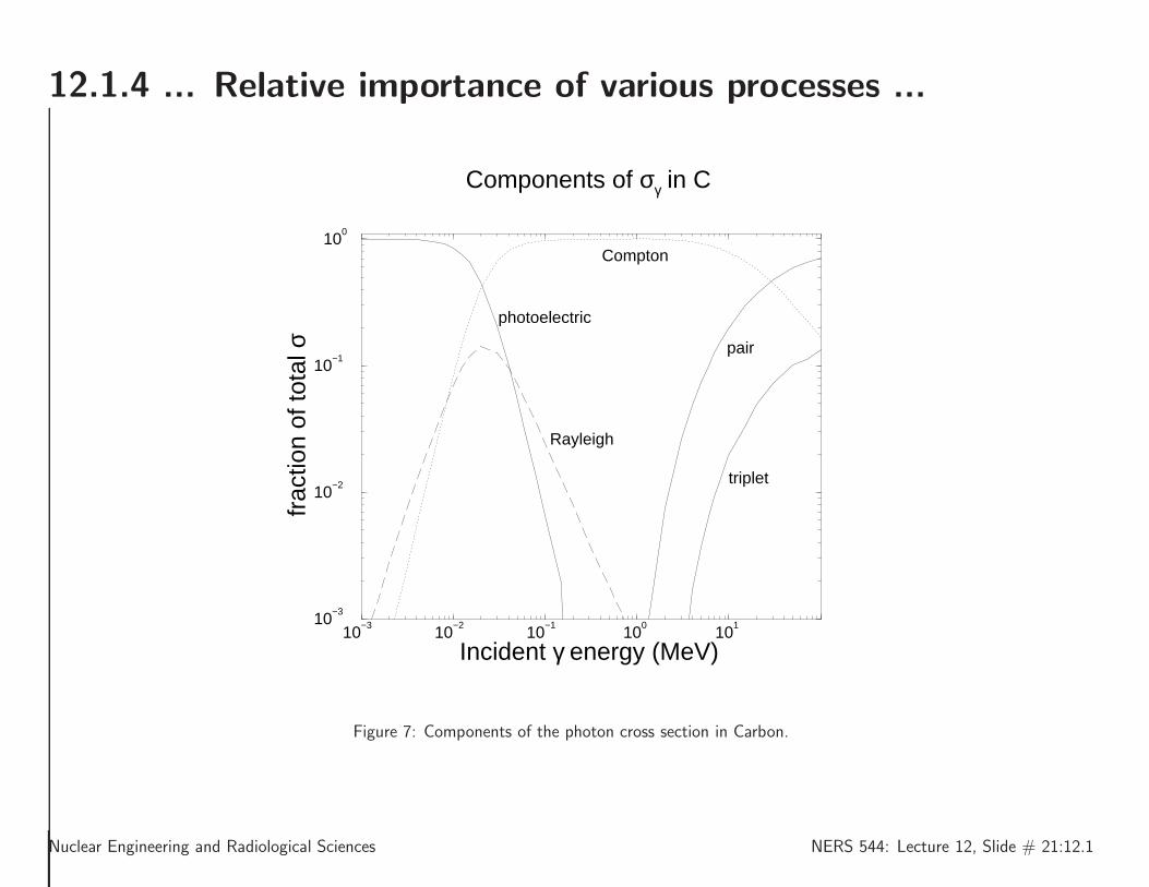
12.1.4 Relative importance of various processes ...

We now consider the relative importance of the various processes involved.

For carbon, a moderately low-Z material, the relative strengths of the photon interactionsversus energy is shown below. For this material we note three distinct regions of singleinteraction dominance:photoelectric below 20 keV,pair above 30 MeV andCompton in between.

The almost order of magnitude depression of the Rayleigh and triplet contributions is somejustification for the relatively crude approximations we have discussed. For lead, shownbelow, there are several differences and many similarities.


12.1.4 ... Relative importance of various processes ...

10−3

10−2

10−1

100

101

Incident γ energy (MeV)10

−3

10−2

10−1

100

frac

tion

of to

tal σ

Components of σγ in C

Compton

photoelectric

Rayleigh

pair

triplet

Figure 7: Components of the photon cross section in Carbon.



10−3

10−2

10−1

100

101


−3

10−2

10−1

100

frac

tion

of to

tal σ

Components of σγ in Pb

Comptonphotoelectric

Rayleigh

pair

triplet

Figure 8: Components of the photon cross section in Lead.



The same comment about the relative unimportance of the Rayleigh and triplet crosssections applies for lead.

The “Compton dominance” section is much smaller, now extending only from 700 keV to4 MeV.

We also note quite a complicated structure below about 90 keV, the K-shell bindingenergy of the lead atom. Below this threshold, atomic structure effects become very im-portant.

Finally, we consider the total cross section versus energy for the materials hydrogen, waterand lead, shown in Figure 9.



10−2

10−1

100

101


−2

10−1

100

101

102

σ (c

m2 /g

)

Total photon σ vs γ−energy

HydrogenWaterLead

Figure 9: Total photon cross section vs. photon energy.



The total cross section is plotted in the units cm2/g.

The Compton dominance regions are equivalent except for a relative A/Z factor.

At high energy the Z2 dependence of pair production is evident in the lead.

At lower energies the Zn(n > 4) dependence of the photoelectric cross section is quiteevident.


12.2 Photon transport logic ...

We now discuss a simplified version of photon transport logic. It is simplified by ignoringelectron creation and considering that the transport occurs in only a single volume elementand a single medium.

This photon transport logic is schematized in the figure below.

An initial photon’s parameters are present at the top of an structure that we shall nameSTACK.

This structure retains particle phase space characteristics for processing.

A transport cutoff is defined. A photons whose energy falls below this cutoff is is consid-ered to be absorbed “on the spot”. (Removed from the STACK.)

We consider that they do not contribute significantly to any tallies of interest and can beignored. Physically, this step is not really necessary—it is only a time-saving maneuver.In “real life” low-energy photons are absorbed by the photoelectric process and vanish.(This is, actually, a bit of a fiction. Energetic discussion to ensue.)


12.3 ... Photon transport logic ...

The logic flow of photon transport proceeds as follows.

A source function places an initial photon on the STACK, defining its energy, direction andposition vector, starting region number, and “weight”.(A particle’s weight is usually assigned to unity, but may have other values based on vari-ance reduction methods, covered in a later chapter.

The photon transport function, described in the following figure, first tests to see if theenergy is below the transport cutoff. If it is below the cutoff, the history is terminated. Ifthe STACK is empty then a new particle history is started.

If the energy is above the cutoff, then the distance to the next interaction site is chosen,following the discussion in Chapter 8, Transport in media, interaction models.


12.4 ... Photon transport logic ...

The photon is then transported, that is transported to the point of interaction. (If thegeometry is more complicated than just one region, transport through different elementsof the geometry would be taken care of here.)

If the photon, by virtue of its transport, has left the volume defining the problem then itis discarded.

Otherwise, the branching distribution is sampled to see which interaction occurs. Havingdone this, the surviving particles (new ones may be created, some disappear, the charac-teristics of the initial one will almost certainly change) have their energies, directions andother characteristics chosen from the appropriate distributions.

The surviving particles are put on the STACK.

Lowest energy ones should be put on the top of the STACK to keep the size of the STACKas small as possible.

Then the whole process takes place again until the STACK is empty and all the incidentparticles are used up.


0.0 0.5 1.00.0

0.5

1.0

Photon Transport

Place initial photon’s parameters on stack

Pick up energy, position, direction, geometry ofcurrent particle from top of stack

Is photon energy < cutoff?

Sample distance to next interactionTransport photon taking geometry into account

Has photon left the volume of interest?

Sample the interaction channel:

Sample energies and directions of resultant particlesand store paramters on stack for future processing

- photoelectric- Compton- pair production- Rayleigh

Is stackempty?

Terminatehistory

NY

Y

N

Y

N

Figure 10: “Bare-bones” photon transport logic.


lecture notes on chapter 12: photon monte carlo simulationumich.edu/~nersa590/lecture12.pdf ·...

Documents