lecture notes on numerical analysis of partial di erential ...arnold/8445.f11/notes.pdf · lecture...
TRANSCRIPT

MATH 8445, University of MinnesotaNumerical Analysis of Differential Equations
Lecture notes on
Numerical Analysis of
Partial Differential Equations
– version of 2011-09-05 –
Douglas N. Arnold
c©2009 by Douglas N. Arnold. These notes may not be duplicated without explicit permission from the author.


Contents
Chapter 1. Introduction 11. Basic examples of PDEs 11.1. Heat flow and the heat equation 11.2. Elastic membranes 31.3. Elastic plates 32. Some motivations for studying the numerical analysis of PDE 4
Chapter 2. The finite difference method for the Laplacian 71. The 5-point difference operator 72. Analysis via a maximum principle 103. Consistency, stability, and convergence 114. Fourier analysis 135. Analysis via summation by parts 156. Extensions 176.1. Curved boundaries 176.2. More general PDEs 206.3. More general boundary conditions 216.4. Nonlinear problems 21
Chapter 3. Linear algebraic solvers 231. Classical iterations 232. The conjugate gradient method 292.1. Line search methods and the method of steepest descents 292.2. The conjugate gradient method 312.3. Preconditioning 383. Multigrid methods 40
Chapter 4. Finite element methods for elliptic equations 491. Weak and variational formulations 492. Galerkin method and finite elements 503. Lagrange finite elements 514. Coercivity, inf-sup condition, and well-posedness 534.1. The symmetric coercive case 544.2. The coercive case 554.3. The inf-sup condition 555. Stability, consistency, and convergence 566. Finite element approximation theory 577. Error estimates for finite elements 62
3

4 CONTENTS
7.1. Estimate in H1 627.2. Estimate in L2 638. A posteriori error estimates and adaptivity 648.1. The Clement interpolant 648.2. The residual and the error 678.3. Estimating the residual 688.4. A posteriori error indicators 698.5. Examples of adaptive finite element computations 70
Chapter 5. Time-dependent problems 751. Finite difference methods for the heat equation 751.1. Forward differences in time 761.2. Backward differences in time 781.3. Fourier analysis 791.4. Crank–Nicolson 792. Finite element methods for the heat equation 802.1. Analysis of the semidiscrete finite element method 812.2. Analysis of a fully discrete finite element method 83

CHAPTER 1
Introduction
Galileo wrote that the great book of nature is written in the language of mathemat-ics. The most precise and concise description of many physical systems is through partialdifferential equations.
1. Basic examples of PDEs
1.1. Heat flow and the heat equation. We start with a typical physical applicationof partial differential equations, the modeling of heat flow. Suppose we have a solid bodyoccupying a region Ω ⊂ R3. The temperature distribution in the body can be given by afunction u : Ω × J → R where J is an interval of time we are interested in and u(x, t) isthe temperature at a point x ∈ Ω at time t ∈ J . The heat content (the amount of thermalenergy) in a subbody D ⊂ Ω is given by
heat content of D =
∫D
cu dx
where c is the product of the specific heat of the material and the density of the material.Since the temperature may vary with time, so can the heat content of D. The change ofheat energy in D from a time t1 to a time t2 is given by
change of heat in D =
∫D
cu(x, t2) dx−∫D
cu(x, t1) dx
=
∫ t2
t1
∂
∂t
∫D
cu dx dt =
∫ t2
t1
∫D
∂(cu)
∂t(x, t) dx dt.
Now, by conservation of energy, any change of heat in D must be accounted for by heatflowing in or out of D through its boundary or by heat entering from external sources (e.g.,if the body were in a microwave oven). The heat flow is measured by a vector field σ(x, t)called the heat flux, which points in the direction in which heat is flowing with magnitudethe rate energy flowing across a unit area per unit time. If we have a surface S embeddedin D with normal n, then the heat flowing across S in the direction pointed to by n in unittime is
∫Sσ · n ds. Therefore the heat that flows out of D, i.e., across its boundary, in the
time interval [t1, t2], is given by
heat flow out of D
∫ t2
t1
∫∂D
σ · n ds dt =
∫ t2
t1
∫D
div σ dx dt,
where we have used the divergence theorem. We denote the heat entering from externalsources by f(x, t), given as energy per unit volume per unit time, so that
∫ t2t1
∫Df(x, t) dx dt
1

2 1. INTRODUCTION
gives amount external heat added to D during [t1, t2], and so conservation of energy isexpressed by the equation
(1.1)
∫ t2
t1
∫D
∂(cu)
∂t(x, t) dx dt = −
∫ t2
t1
∫D
div σ ds dt+
∫ t2
t1
∫D
f(x, t) dx dt,
for all subbodies D ⊂ Ω and times t1, t2. Thus the quantity
∂(cu)
∂t+ div σ − f
must vanish identically, and so we have established the differential equation
∂(cu)
∂t= − div σ + f, x ∈ Ω,∀t.
To complete the description of heat flow, we need a constitutive equation, which tellsus how the heat flux depends on the temperature. The simplest is Fourier’s law of heatconduction, which says that heat flows in the direction opposite the temperature gradientwith a rate proportional to the magnitude of the gradient:
σ = −λ gradu,
where the positive quantity λ is called the conductivity of the material. (Usually λ is justa scalar, but if the material is thermally anisotropic, i.e., it has preferred directions of heatflow, as might be a fibrous or laminated material, λ can be a 3× 3 positive-definite matrix.)Therefore we have obtained the equation
∂(cu)
∂t= div(λ gradu) + f in Ω× J.
The source function f , the material coefficients c and λ and the solution u can all be functionsof x and t. If the material is homogeneous (the same everywhere) and not changing withtime, then c and λ are constants and the equation simplifies to the heat equation,
µ∂u
∂t= ∆u+ f ,
where µ = c/λ and we have f = f/λ. If the material coefficients depend on the temperatureu, as may well happen, we get a nonlinear PDE generalizing the heat equation.
The heat equation not only governs heat flow, but all sorts of diffusion processes wheresome quantity flows from regions of higher to lower concentration. The heat equation is theprototypical parabolic differential equation.
Now suppose our body reaches a steady state: the temperature is unchanging. Then thetime derivative term drops and we get
(1.2) − div(λ gradu) = f in Ω,
where now u and f are functions of f alone. For a homogeneous material, this becomes thePoisson equation
−∆u = f ,
the prototypical elliptic differential equation. For an inhomogeneous material we can leavethe steady state heat equation in divergence form as in (1.2), or differentiate out to obtain
−λ∆u+ gradλ · gradu = f.

1. BASIC EXAMPLES OF PDES 3
To determine the steady state temperature distribution in a body we need to know notonly the sources and sinks within the body (given by f), but also what is happening at theboundary Γ := ∂Ω. For example a common situation is that the boundary is held at a giventemperature
(1.3) u = g on Γ.
The PDE (1.2) together with the Dirichlet boundary condition (1.3) form an elliptic bound-ary value problem. Under a wide variety of circumstances this problem can be shown tohave a unique solution. The following theorem is one example (although the smoothnessrequirements can be greatly relaxed).
Theorem 1.1. Let Ω be a smoothly bounded domain in Rn, and let λ : Ω→ R+, f : Ω→R, g : Γ → R be C∞ functions. Then there exists a unique function u ∈ C2(Ω) satisfyingthe differential equation (1.2) and the boundary condition (1.3). Moreover u is C∞.
Instead of the Dirichlet boundary condition of imposed temperature, we often see theNeumann boundary condition of imposed heat flux (flow across the boundary):
∂u
∂n= g on Γ.
For example if g = 0, this says that the boundary is insulated. We may also have a Dirichletcondition on part of the boundary and a Neumann condition on another.
1.2. Elastic membranes. Consider a taut (homogeneous isotropic) elastic membraneaffixed to a flat or nearly flat frame and possibly subject to a transverse force distribution,e.g., a drum head hit by a mallet. We model this with a bounded domain Ω ⊂ R2 whichrepresents the undisturbed position of the membrane if the frame is flat and no force isapplied. At any point x of the domain and any time t, the transverse displacement isgiven by u(x, t). As long as the displacements are small, then u approximately satisfies themembrane equation
ρ∂2u
∂t2= k∆u+ f,
where ρ is the density of the membrane (mass per unit area), k is the tension (force perunit distance), and f is the imposed transverse force density (force per unit area). This isa second order hyperbolic equation, the wave equation. If the membrane is in steady state,the displacement satisfies the Poisson equation
−∆u = f ,
f = f/k.
1.3. Elastic plates. The derivation of the membrane equation depends upon the as-sumption that the membrane resists stretching (it is under tension), but does not resistbending. If we consider a plate, i.e., a thin elastic body made of a material which resistsbending as well as stretching, we obtain instead the plate equation
ρ∂2u
∂t2= −D∆2u+ f,

4 1. INTRODUCTION
where D is the bending modulus, a constant which takes into account the elasticity of thematerial and the thickness of the plate (D = Et3/[12(1− ν2)] where E is Young’s modulusand ν is Poisson’s ratio). Now the steady state equation is the biharmonic equation
∆2u = f .
Later in this course we will study other partial differential equations, including the equa-tions of elasticity, the Stokes and Navier–Stokes equations of fluid flow, and Maxwell’s equa-tions of electromagnetics.
2. Some motivations for studying the numerical analysis of PDE
In this course we will study algorithms for obtaining approximate solutions to PDEproblems, for example, using the finite element method. Such algorithms are a hugelydeveloped technology (we will, in fact, only skim the surface of what is known in this course),and there are thousands of computer codes implementing them. As an example of the sort ofwork that is done routinely, here is the result of a simulation using a finite element methodto find a certain kind of force distribution, the so-called von Mises stress, engendered in aconnecting rod of a Porsche race car when a certain load is applied. The von Mises stresspredicts when and where the metal of the rod will deform, and was used to design the shapeof the rod.
Figure 1.1. Connector rods designed by LN Engineering for Porsche racecars, and the stress distribution in a rod computed with finite elements.
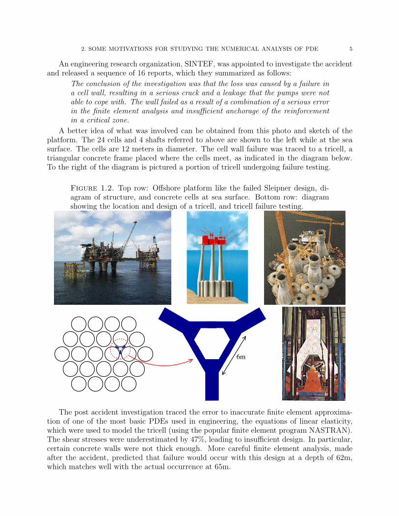
But one should not get the idea that it is straightforward to solve any reasonable PDEproblem with finite elements. Not only do challenges constantly arise as practitioners seekto model new systems and solve new equations, but when used with insufficient knowledgeand care, even advance numerical software can give disastrous results. A striking exampleis the sinking of the Sleipner A offshore oil platform in the North Sea in 1991. This occuredwhen the Norwegian oil company, Statoil, was slowly lowering to the sea floor an arrayof 24 massive concrete tanks, which would support the 57,000 ton platform (which was toaccomodate about 200 people and 40,000 tons of drilling equipment). By flooding the tanksin a so-called controlled ballasting operation, they were lowered at the rate of about 5 cmper minute. When they reached a depth of about 65m the tanks imploded and crashed tothe sea floor, leaving nothing but a pile of debris at 220 meters of depth. The crash did notresult in loss of life, but did cause a seismic event registering 3.0 on the Richter scale, andan economic loss of about $700 million.
2. SOME MOTIVATIONS FOR STUDYING THE NUMERICAL ANALYSIS OF PDE 5
An engineering research organization, SINTEF, was appointed to investigate the accidentand released a sequence of 16 reports, which they summarized as follows:
The conclusion of the investigation was that the loss was caused by a failure ina cell wall, resulting in a serious crack and a leakage that the pumps were notable to cope with. The wall failed as a result of a combination of a serious errorin the finite element analysis and insufficient anchorage of the reinforcementin a critical zone.
A better idea of what was involved can be obtained from this photo and sketch of theplatform. The 24 cells and 4 shafts referred to above are shown to the left while at the seasurface. The cells are 12 meters in diameter. The cell wall failure was traced to a tricell, atriangular concrete frame placed where the cells meet, as indicated in the diagram below.To the right of the diagram is pictured a portion of tricell undergoing failure testing.
Figure 1.2. Top row: Offshore platform like the failed Sleipner design, di-agram of structure, and concrete cells at sea surface. Bottom row: diagramshowing the location and design of a tricell, and tricell failure testing.
6m
The post accident investigation traced the error to inaccurate finite element approxima-tion of one of the most basic PDEs used in engineering, the equations of linear elasticity,which were used to model the tricell (using the popular finite element program NASTRAN).The shear stresses were underestimated by 47%, leading to insufficient design. In particular,certain concrete walls were not thick enough. More careful finite element analysis, madeafter the accident, predicted that failure would occur with this design at a depth of 62m,which matches well with the actual occurrence at 65m.


CHAPTER 2
The finite difference method for the Laplacian
With the motivation of the previous section, let us consider the numerical solution of theelliptic boundary value problem
(2.1) ∆u = f in Ω, u = g on Γ.
For simplicity we will consider first a very simple domain Ω = (0, 1)× (0, 1), the unit squarein R2. Now this problem is so simplified that we can attack it analytically, e.g., by separationof variables, but it is a very useful model problem for studying numerical methods.
1. The 5-point difference operator
Let N be a positive integer and set h = 1/N . Consider the mesh in R2
R2h := (mh, nh) : m,n ∈ Z .
Note that each mesh point x ∈ R2h has four nearest neighbors in R2
h, one each to the left,right, above, and below. We let Ωh = Ω∩R2
h, the set of interior mesh points, and we regardthis a discretization of the domain Ω. We also define Γh as the set of mesh points in R2
h
which don’t belong to Ωh, but which have a nearest neighbor in Ωh. We regard Γh as adiscretization of Γ. We also let Ωh := Ωh ∪ Γh
To discretize (2.1) we shall seek a function uh : Ωh → R satisfying
(2.2) ∆h uh = f on Ωh, uh = g on Γh.
Here ∆h is an operator, to be defined, which takes functions on Ωh (mesh functions) tofunctions on Ωh. It should approximate the true Laplacian in the sense that if v is a smoothfunction on Ω and vh = v|Ωh
is the associated mesh function, then we want
∆h vh ≈ ∆ v|Ωh
for h small.Before defining ∆h, let us turn to the one-dimensional case. That is, given a function vh
defined at the mesh points nh, n ∈ Z, we want to define a function D2hvh on the mesh points,
so that D2hvh ≈ v′′|Zh if vh = v|Zh. One natural procedure is to construct the quadratic
polynomial p interpolating vh at three consecutive mesh points (n− 1)h, nh, (n + 1)h, andlet D2
hvh(nh) be the constant value of p′′. This gives the formula
D2hvh(nh) = 2vh[(n− 1)h, nh, (n+ 1)h] =
vh((n+ 1)h
)− 2vh(nh) + vh
((n− 1)h
)h2
.
D2h is known as the 3-point difference approximation to d2/dx2. We know that if v is C2 in
a neighborhood of nh, then limh→0 v[x − h, x, x + h] = v′′(x)/2. In fact, it is easy to show
7

8 2. THE FINITE DIFFERENCE METHOD FOR THE LAPLACIAN
Figure 2.1. Ωh for h = 1/14: black: points in Ωh, purple: points in Γh.
by Taylor expansion (do it!), that
D2hv(x) = v′′(x) +
h2
12v(4)(ξ), for some ξ ∈
(x− h, x+ h
),
as long as v is C4 near x. Thus D2h is a second order approximation to d2/dx2.
Now returning to the definition of the ∆h ≈ ∆ = ∂2/∂x2 + ∂2/∂y2, we simply use the3-point approximation to ∂2/∂x2 and ∂2/∂y2. Writing vmn for v(mh, nh) we then have
∆h v(mh, nh) =vm+1,n − 2vmn + vm−1,n
h2+vm,n+1 − 2vmn + vm,n−1
h2
=vm+1,n + vm−1,n + vm,n+1 + vm,n−1 − 4vmn
h2.
From the error estimate in the one-dimensional case we easily get that for v ∈ C4(Ω),
∆h v(mh, nh)−∆ v(mh, nh) =h2
12
[∂4v
∂x4(ξ, nh) +
∂4v
∂y4(mh, η)
],
for some ξ, η. Thus:
Theorem 2.1. If v ∈ C2(Ω), then
limh→0‖∆h v −∆ v‖L∞(Ωh) = 0.
1. THE 5-POINT DIFFERENCE OPERATOR 9
If v ∈ C4(Ω), then
‖∆h v −∆ v‖L∞(Ωh) ≤h2
6M4,
where M4 = max(‖∂4v/∂x4‖L∞(Ω), ‖∂4v/∂y4‖L∞(Ω)).
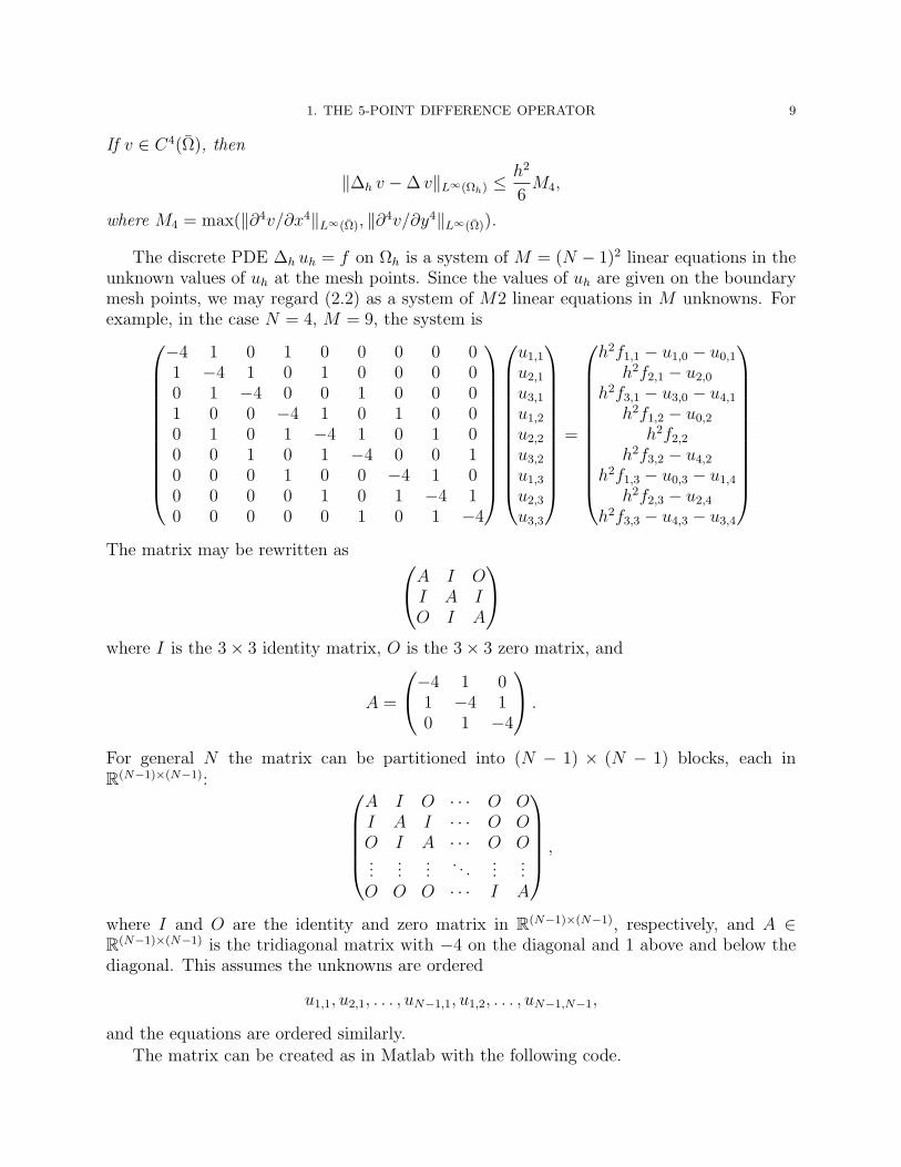
The discrete PDE ∆h uh = f on Ωh is a system of M = (N − 1)2 linear equations in theunknown values of uh at the mesh points. Since the values of uh are given on the boundarymesh points, we may regard (2.2) as a system of M2 linear equations in M unknowns. Forexample, in the case N = 4, M = 9, the system is
−4 1 0 1 0 0 0 0 01 −4 1 0 1 0 0 0 00 1 −4 0 0 1 0 0 01 0 0 −4 1 0 1 0 00 1 0 1 −4 1 0 1 00 0 1 0 1 −4 0 0 10 0 0 1 0 0 −4 1 00 0 0 0 1 0 1 −4 10 0 0 0 0 1 0 1 −4
u1,1
u2,1
u3,1
u1,2
u2,2
u3,2
u1,3
u2,3
u3,3
=
h2f1,1 − u1,0 − u0,1
h2f2,1 − u2,0
h2f3,1 − u3,0 − u4,1
h2f1,2 − u0,2
h2f2,2
h2f3,2 − u4,2
h2f1,3 − u0,3 − u1,4
h2f2,3 − u2,4
h2f3,3 − u4,3 − u3,4
The matrix may be rewritten as A I O
I A IO I A
where I is the 3× 3 identity matrix, O is the 3× 3 zero matrix, and
A =
−4 1 01 −4 10 1 −4
.
For general N the matrix can be partitioned into (N − 1) × (N − 1) blocks, each inR(N−1)×(N−1):
A I O · · · O OI A I · · · O OO I A · · · O O...
......
. . ....
...O O O · · · I A
,
where I and O are the identity and zero matrix in R(N−1)×(N−1), respectively, and A ∈R(N−1)×(N−1) is the tridiagonal matrix with −4 on the diagonal and 1 above and below thediagonal. This assumes the unknowns are ordered
u1,1, u2,1, . . . , uN−1,1, u1,2, . . . , uN−1,N−1,
and the equations are ordered similarly.The matrix can be created as in Matlab with the following code.

10 2. THE FINITE DIFFERENCE METHOD FOR THE LAPLACIAN
I = speye(n-1);
e = ones(n-1,1);
A = spdiags([e,-4*e,e],[-1,0,1],n-1,n-1);
J = spdiags([e,e],[-1,1],n-1,n-1);
Lh = kron(I,A) + kron(J,I)
Notice that the matrix has many special properties:
• it is sparse with at most 5 elements per row nonzero• it is block tridiagonal, with tridiagonal and diagonal blocks• it is symmetric• it is diagonally dominant• its diagonal elements are negative, all others nonnegative• it is negative definite
2. Analysis via a maximum principle
We will now prove that the problem (2.2) has a unique solution and prove an errorestimate. The key will be a discrete maximum principle.
Theorem 2.2 (Discrete Maximum Principle). Let v be a function on Ωh satisfying
∆h v ≥ 0 on Ωh.
Then maxΩhv ≤ maxΓh
v. Equality holds if and only if v is constant.
Proof. Suppose maxΩhv ≥ maxΓh
v. Take x0 ∈ Ωh where the maximum is achieved.Let x1, x2, x3, and x4 be the nearest neighbors. Then
4v(x0) =4∑i=1
v(xi)− h2 ∆h v(x0) ≤4∑i=1
v(xi) ≤ 4v(x0),
since v(xi) ≤ v(x0). Thus equality holds throughout and v achieves its maximum at all thenearest neighbors of x0 as well. Applying the same argument to the neighbors in the interior,and then to their neighbors, etc., we conclude that v is constant.
Remarks. 1. The analogous discrete minimum principle, obtained by reversing the in-equalities and replacing max by min, holds. 2. This is a discrete analogue of the maximumprinciple for the Laplace operator.
Theorem 2.3. There is a unique solution to the discrete boundary value problem (2.2).
Proof. Since we are dealing with a square linear system, it suffices to show nonsingu-larity, i.e., that if ∆h uh = 0 on Ωh and uh = 0 on Γh, then uh ≡ 0. Using the discretemaximum and the discrete minimum principles, we see that in this case uh is everywhere0.
The next result is a statement of maximum norm stability.
Theorem 2.4. The solution uh to (2.2) satisfies
(2.3) ‖uh‖L∞(Ωh) ≤1
8‖f‖L∞(Ωh) + ‖g‖L∞(Γh).

3. CONSISTENCY, STABILITY, AND CONVERGENCE 11
This is a stability result in the sense that it states that the mapping (f, g) 7→ uh isbounded uniformly with respect to h.
Proof. We introduce the comparison function φ(x) = [(x1 − 1/2)2 + (x2 − 1/2)2]/4,which satisfies ∆h φ = 1 on Ωh, and 0 ≤ φ ≤ 1/8 on Ωh. Set M = ‖f‖L∞(Ωh). Then
∆h(uh +Mφ) = ∆h uh +M ≥ 0,
so
maxΩh
uh ≤ maxΩh
(uh +Mφ) ≤ maxΓh
(uh +Mφ) ≤ maxΓh
g +1
8M.
Thus uh is bounded above by the right-hand side of (2.3). A similar argument applies to−uh giving the theorem.
By applying the stability result to the error u − uh we can bound the error in terms ofthe consistency error ∆h u−∆u.
Theorem 2.5. Let u be the solution of the Dirichlet problem (1.2) and uh the solutionof the discrete problem (2.2). Then
‖u− uh‖L∞(Ωh) ≤1
8‖∆u−∆h u‖L∞(Ωh).
Proof. Since ∆h uh = f = ∆u on Ωh, ∆h(u − uh) = ∆h u −∆u. Also, u − uh = 0 onΓh. Apply Theorem 2.4 (with uh replaced by u− uh), we obtain the theorem.
Combining with Theorem 2.1, we obtain error estimates.
Corollary 2.6. If u ∈ C2(Ω), then
limh→0‖u− uh‖L∞(Ωh) = 0.
If u ∈ C4(Ω), then
‖u− uh‖L∞(Ωh) ≤h2
48M4,
where M4 = max(‖∂4u/∂x41‖L∞(Ω), ‖∂4u/∂x4
2‖L∞(Ω)).
3. Consistency, stability, and convergence
Now we introduce an abstract framework in which to understand the preceding analysis.It is general enough that it applies, or can be adapted to, a huge variety of numerical methodsfor PDE. We will keep in mind, as an basic example, the 5-point difference discretizationof the Poisson equation with homogeneous boundary conditions, so the PDE problem to besolved is
∆u = f in Ω, u = 0 on Γ,
and the numerical method is
∆huh = fh in Ωh, uh = 0 on Γh.
Let X and Y be vector spaces and L : X → Y a linear operator. Given f ∈ Y , we seeku ∈ X such that Lu = f . This is the problem we are trying to solve. So, for the homogeneousDirichlet BVP for Poisson’s equation, we could take X to be the space of C2 functions onΩ which vanish on Γ, Y = C(Ω), and L = ∆. (Actually, slightly more sophisticated spaces

12 2. THE FINITE DIFFERENCE METHOD FOR THE LAPLACIAN
should be taken if we wanted to get a good theory for the Poisson equation, but that won’tconcern us now.) We shall assume that there is a solution u of the original problem.
Now let Xh and Yh be finite dimensional normed vector spaces and Lh : Xh → Yh a linearoperator. Our numerical method, or discretization, is:
Given fh ∈ Yh find uh ∈ Xh such that Lhuh = fh.
Of course, this is a very minimalistic framework so far. Without some more hypotheses, wedo not know if this finite dimensional problem has a solution, or if the solution is unique.And we certainly don’t know that uh is in any sense an approximation of u.
In fact, up until now, there is no way to compare u to uh, since they belong to differentspaces. For this reason, we introduce a representative of u, rhu ∈ Xh. We can then talkabout the error rhu−uh and its norm ‖rhu−uh‖Xh
. If this error norm is small, that meansthat uh is close to u, or at least close to our representative rhu of u, in the sense of the norm.
In short, we would like the error to be small in norm. To make this precise we do whatis always done in numerical analysis: we consider not a single discretization, but a sequenceof discretizations. To keep the notation simple, we will now think of h > 0 as a parametertending to 0, and suppose that we have the normed spaces Xh and Yh and the linear operatorLh : Xh → Yh and the element fh ∈ Yh for each h. This family of discretizations is calledconvergent if the norm ‖rhu− uh‖Xh
tends to 0 as h→ 0.In our example, we take Xh to be the grid functions in L∞(Ωh) which vanish on Γh, and
Yh to be the grid functions in L∞(Ω), and equip both with the maximum norm. We alsosimply define rhu = u|Ωh
. Thus a small error means that uh is close to the true solution uat all the grid points, which is a desireable result.
Up until this point there is not enough substance to our abstract framework for us to beable to prove a convergence result, because the only connection between the original problemLu = f and the discrete problems Lhuh = fh is that the notations are similar. We surelyneed some hypotheses. The first of two key hypotheses is consistency, which say that, insome sense, the discrete problem is reasonable, in that the solution of the original problemalmost satisfies the discrete problem. More precisely, we define the consistency error asLhrhu − fh ∈ Yh, a quantity which we can measure using our norm in Yh. The family ofdiscretizations is called consistent if the norm ‖Lhrhu− fh‖Yh
tends to 0 as h→ 0.Not every consistent family of discretizations is convergent (as you can easily convince
yourself, since consistency involves the norm in Yh but not the norm in Xh and for con-vergence it is the opposite). There is a second key hypothesis, uniform well-posedness ofthe discrete problems. More precisely, we assume that each discrete problem is uniquelysolvable (nonsingular): for every gh ∈ Yh there is a unique vh ∈ Xh with Lhvh = gh. Thusthe operator L−1
h : Yh → Xh is defined and we call its norm ch = ‖L−1h ‖L(Yh,Xh) the stability
constant of the discretization. The family of discretizations is called stable if the stabilityconstants are bounded uniformly in h: suph ch <∞. Note that stability is a property of thediscrete problems and depends on the particular choice of norms, but it does not depend onthe true solution u in any way.
With these definition we get a theorem which is trivial to prove, but which captures theunderlying structure of many convergence results in numerical PDE.
Theorem 2.7. Let there be given normed vector spaces Xh and Yh, an invertible linearoperator Lh : Xh → Yh, an element fh ∈ Yh, and a representative rhu ∈ Xh. Define uh ∈ Xh

4. FOURIER ANALYSIS 13
by Lhuh = fh. Then the norm of the error is bounded by the stability constant times thenorm of the consistency error. If a family of such discretizations is consistent and stable,then it is convergent.
Proof. Since Lhuh = fh,
Lh(rhu− uh) = Lhrhu− fh.Applying L−1
h we obtain
rhu− uh = L−1h (Lhrhu− fh),
and taking norms we get
‖rhu− uh‖Xh= ‖L−1
h ‖L(Yh,Xh)‖Lhrhu− fh‖Yh,
which is the desired result.
Remark. We emphasize that the concepts of convergence, consistency, and stabilitydepend on the choice of norms in Xh, Yh, and both, respectively. The norm in Xh shouldbe chosen so that the convergence result gives information that is desired. Choosing a weaknorm may make the hypotheses easier to verify, but the result of less interest. Similarly, fhmust be chosen in a practical way. We need fh to compute uh, so it should be something weknow before we solve the problem, typically something easily computed from f . Similarly aswell, rhu should be chosen in a reasonable way. For example, choosing rhu = L−1
h fh wouldgive rhu = uh so we definitely have a convergent method, but this is cheating: convergence isof no interest with this choice. The one other choice we have at our disposal is the norm onYh. This we are free to choose in order to make the hypotheses of consistency and stabilitypossible to verify. Note that weakening the norm on Yh makes it easier to prove consistency,while strengthening it makes it easier to prove stability.
Returning to our example, we see that the first statement of Theorem 2.1 is just thestatement that the method is consistent for any solution u ∈ C2(Ω), and the second statementsays that the consistency error is O(h2) if u ∈ C4(Ω). On the other hand, if we applyTheorem 2.4 with g = 0, it states that the stability constant ch ≤ 1/8 for all h, and so themethod is stable. We then obtain the convergence result in Corollary 2.6 by the basic resultof Theorem 2.7.
4. Fourier analysis
Define L(Ωh) to be the set of functions Ωh → R, which is isomorphic to RM , M = (N−1)2.Sometimes we think of these as functions on Ωh extended by zero to Γh. The discreteLaplacian then defines an isomorphism of L(Ωh) onto itself. As we just saw, the L∞ stabilityconstant, ‖∆−1
h ‖L(L∞,L∞) ≤ 1/8. In this section we use Fourier analysis to establish a similarL2 stability result.
First consider the one-dimensional case. With h = 1/N let Ih = h, 2h, . . . , (N − 1)h,and let L(Ih) be the space of functions on Ih, which is an N − 1 dimensional vectorspace.On L(Ih) we define the inner product
〈u, v〉h = hN−1∑k=1
u(kh)v(kh),

14 2. THE FINITE DIFFERENCE METHOD FOR THE LAPLACIAN
with the corresponding norm ‖v‖h.The space L(Ih) is a discrete analogue of L2(I) where I is the unit interval. On this
latter space the functions sinπmx, m = 1, 2, . . ., form an orthogonal basis consisting ofeigenfunctions of the operator −d2/dx2. The corresponding eigenvalues are π2, 4π2, 9π2, . . ..We now establish the discrete analogue of this result.
Define φm ∈ L(Ih) by φm(x) = sinπmx, x ∈ Ih. It turns out that these mesh functionsare precisely the eigenvectors of the operator D2
h. Indeed
D2hφm(x) =
sin πm(x+ h)− 2 sinπmx+ sin πm(x− h)
h2=
2
h2(cos πmh− 1) sinπmx.
Thus
D2hφm = −λmφm, λm =
2
h2(1− cos πmh) =
4
h2sin2 πmh
2.
Note that
0 < λ1 < λ2 < · · · < λN−1 <4
h2.
Note also that for small m << N , λm ≈ π2m2. In particular λ1 ≈ π2. To get a strict lowerbound we note that λ1 = 8 for N = 2 and λ1 increases with N .
Since the operator D2h is symmetric with respect to the inner product on L(Ih), and the
eigenvalues λm are distinct, it follows that the eigenvectors φm are mutually orthogonal.(This can also be obtained using trigonometric identities, or by expressing the sin functionsin terms of complex exponentials and using the discrete Fourier transform.) Since there areN − 1 of them, they form a basis of L(Ih).
Theorem 2.8. The functions φm, m = 1, 2, . . . , N − 1 form an orthogonal basis ofL(Ih). Consequently, any function v ∈ L(Ih) can be expanded as v =
∑N−1m=1 amφm with
am = 〈v, φm〉h/‖φm‖2h, and ‖v‖2
h =∑N−1
m=1 a2m‖φm‖2
h.
From this we obtain immediately a stability result for the one-dimensional Laplacian. Ifv ∈ L(Ih) and D2
hv = f , we expand v in terms of the φm:
v =N−1∑m=1
amφm, ‖v‖2h =
N−1∑m=1
a2m‖φm‖2
h.
Then
f = −N−1∑m=1
λmamφm, ‖f‖2h =
N−1∑m=1
λ2ma
2m‖φm‖2
h ≥ 82‖v‖2h.
Thus ‖v‖h ≤ ‖f‖h/8.The extension to the two-dimensional case is straightforward. We use the basis φmn =
φm ⊗ φn, i.e.,
φmn(x, y) := φm(x)φn(y), m, n = 1, . . . , N − 1,
for L(Ωh). It is easy to see that these (N − 1)2 functions form an orthogonal basis for L(Ωh)equipped with the inner product
〈u, v〉h = h2
N−1∑m=1
N−1∑n=1
u(mh, nh)v(mh, nh)

5. ANALYSIS VIA SUMMATION BY PARTS 15
and corresponding norm ‖ · ‖h. Moreover φmn is an eigenvector of −∆h with eigenvalueλmn = λm + λn ≥ 16. The next theorem follows immediately.
Theorem 2.9. The operator ∆h defines an isomorphism from L(Ωh) to itself. Moreover‖∆−1
h ‖ ≤ 1/16 where the operator norm is with respect to the norm ‖ · ‖h on L(Ωh).
Since the ‖v‖h ≤ ‖v‖L∞(Ωh) we also have consistency with respect to the discrete 2-norm.We leave it to the reader to complete the analysis with a convergence result.
5. Analysis via summation by parts
Fourier analysis is not the only approach to get an L2 stability result. Another usessummation by parts, the discrete analogue of integration by parts.
Let v be a mesh function. Define the backward difference operator
∂xv(mh, nh) =v(mh, nh)− v((m− 1)h, nh)
h, 1 ≤ m ≤ N, 0 ≤ n ≤ N.
In this section we denote
〈v, w〉h = h2
N∑m=1
N∑n=1
v(mh, nh)w(mh, nh),
with the corresponding norm ‖ · ‖h (this agrees with the notation in the last section for meshfunctions which vanish on Γh).
Lemma 2.10. If v ∈ L(Ωh) (the set of mesh functions vanishing on Γh), then
‖v‖h ≤1
2(‖∂xv‖h + ‖∂yv‖h).
Proof. It is enough to show that ‖v‖h ≤ ‖∂xv‖h. The same will similarly hold for ∂y aswell, and we can average the two results.
For 1 ≤ m ≤ N , 0 ≤ n ≤ N ,
|v(mh, nh)|2 ≤
(N∑i=1
|v(ih, nh)− v((i− 1)h, nh)|
)2
=
(h
N∑i=1
|∂xv(ih, nh)|
)2
≤
(h
N∑i=1
|∂xv(ih, nh)|2)(
hN∑i=1
12
)
= h
N∑i=1
|∂xv(ih, nh)|2.
Therefore
h
N∑m=1
|v(mh, nh)|2 ≤ h
N∑i=1
|∂xv(ih, nh)|2

16 2. THE FINITE DIFFERENCE METHOD FOR THE LAPLACIAN
and
h2
N∑m=1
N∑n=1
|v(mh, nh)|2 ≤ h2
N∑i=1
N∑n=1
|∂xv(ih, nh)|2,
i.e., ‖v‖2h ≤ ‖∂xv‖2
h, as desired.
This result is a discrete analogue of Poincare’s inequality, which bounds a function interms of its gradient as long as the function vanishes on a portion of the boundary. Theconstant of 1/2 in the bound can be improved. The next result is a discrete analogue ofGreen’s Theorem (essentially, integration by parts).
Lemma 2.11. If v, w ∈ L(Ωh), then
−〈∆h v, w〉h = 〈∂xv, ∂xw〉h + 〈∂yv, ∂yw〉h.
Proof. Let v0, v1, . . . , vN , w0, w1, . . . , wN ∈ R with w0 = wN = 0. Then
N∑i=1
(vi − vi−1)(wi − wi−1) =N∑i=1
viwi +N∑i=1
vi−1wi−1 −N∑i=1
vi−1wi −N∑i=1
viwi−1
= 2N−1∑i=1
viwi −N−1∑i=1
vi−1wi −N−1∑i=1
vi+1wi
= −N−1∑i=1
(vi+1 − 2vi + vi−1)wi.
Hence,
− hN−1∑i=1
v((i+ 1)h, nh)− 2v(ih, nh) + v((i− 1)h, nh)
h2w(ih, nh)
= h
N∑i=1
∂xv(ih, nh)∂xw(ih, nh),
and thus
−〈D2xv, w〉h = 〈∂xv, ∂xw〉h.
Similarly, −〈D2yv, w〉h = 〈∂yv, ∂yw〉h, so the lemma follows.
Combining the discrete Poincare inequality with the discrete Green’s theorem, we imme-diately get a stability result. If v ∈ L(Ωh), then
‖v‖2h ≤
1
2(‖∂xv‖2
h + ‖∂yv‖2h) = −1
2〈∆h v, v〉h ≤
1
2‖∆h v‖h‖v‖h.
Thus
‖v‖h ≤ ‖∆h v‖h, v ∈ L(Ωh),
which is a stability result.

6. EXTENSIONS 17
Figure 2.2. Gray points: Ωh. Black points: Ω∂h. Blue points: Γh.
6. Extensions
6.1. Curved boundaries. Thus far we have studied as a model problem the discretiza-tion of Poisson’s problem on the square. In this subsection we consider a variant which canbe used to discretize Poisson’s problem on a fairly general domain.
Let Ω be a smoothly bounded open set in R2 with boundary Γ. We again consider theDirichlet problem for Poisson’s equation, (2.1), and again set Ωh = Ω ∩ R2
h. If (x, y) ∈ Ωh
and the segment (x+ sh, y), 0 ≤ s ≤ 1 belongs to Γ, then the point (x+h, y), which belongsto Ωh, is a neighbor of (x, y) to the right. If this segment doesn’t belong to Ω we defineanother sort of neighbor to the right, which belongs to Γ. Namely we define the neighbor tobe the point (x + sh, y) where 0 < s ≤ 1 is the largest value for which (x + th, y) ∈ Ω forall 0 ≤ t < s. The points of Γ so constructed (as neighbors to the right or left or above orbelow points in Ωh) constitute Γh. Thus every point in Ωh has four nearest neighbors all of
which belong to Ωh := Ωh ∪ Γh. We also define Ωh as those points in Ωh all four of whoseneighbor belong to Ωh and Ω∂
h as those points in Ωh with at least one neighbor in Γh. SeeFigure 2.2.
In order to discretize the Poisson equation we need to construct a discrete analogue ofthe Laplacian ∆h v for mesh functions v on Ωh. Of course on Ωh, ∆h v is defined as the usual5-point Laplacian. For (x, y) ∈ Ω∂
h, let (x+h1, y), (x, y+h2), (x−h3, y), and (x, y−h4) be thenearest neighbors (with 0 < hi ≤ h), and let v1, v2, v3, and v4 denote the value of v at thesefour points. Setting v0 = v(x, y) as well, we will define ∆h v(x, y) as a linear combination ofthe five values vi. In order to derive the formula, we first consider approximating d2v/dx2(0)by a linear combination of v(−h−), v(0), and v(h+), for a function v of one variable. ByTaylor’s theorem
α−v(−h−) + α0v(0) + α+v(h+) = (α− + α0 + α+)v(0) + (α+h+ − α−h−)v′(0)
+1
2(α+h
2+ + α−h
2−)v′′(0) +
1
6(α+h
3+ − α−h3
−)v′′′(0) + · · · .

18 2. THE FINITE DIFFERENCE METHOD FOR THE LAPLACIAN
Thus, to obtain a consistent approximation we must have
α− + α0 + α+ = 0, α+h+ − α−h− = 0,1
2(α+h
2+ + α−h
2−) = 1,
which give
α− =2
h−(h− + h+), α+ =
2
h+(h− + h+), α0 =
−2
h−h+
.
Note that we have simply recovered the usual divided difference approximation to d2v/dx2:
α−v(−h−)+α0v(0)+α+v(h+) =[v(h+)− v(0)]/h+ − [v(0)− v(−h−)]/h−
(h+ + h−)/2= 2v[−h−, 0, h+].
Returning to the 2-dimensional case, and applying the above considerations to both∂2v/∂x2 and ∂2v/∂y2 we arrive at the Shortley–Weller formula for ∆h v:
∆h v(x, y)
=2
h1(h1 + h3)v1 +
2
h2(h2 + h4)v2 +
2
h3(h1 + h3)v3 +
2
h4(h2 + h4)v4 −
(2
h1h3+
2
h2h4
)v0.
Using Taylor’s theorem with remainder we easily calculate that for v ∈ C3(Ω),
‖∆ v −∆h v‖L∞(Ωh) ≤2M3
3h,
where M3 is the maximum of the L∞ norms of the third derivatives of v. Of course at themesh points in Ωh, the truncation error is bounded by M4h
2/6 = O(h2), as before, but formesh points neighboring the boundary, it is reduced to O(h).
The approximate solution to (2.1) is uh : Ωh → R determined again by 2.2. This is asystem of linear equations with one unknown for each point of Ωh. In general the matrixwon’t be symmetric, but it maintains other good properties from the case of the square:
• it is sparse, with at most five elements per row• it has negative diagonal elements and non-negative off-diagonal elements• it is diagonally dominant.
Using these properties we can obtain the discrete maximum principle with virtually the sameproof as for Theorem 2.2, and then a stability result as in Theorem 2.4 follows as before. Inthis way we can easily obtain an O(h) convergence result.
However, we can improve this result by modifying our previous analysis. Although thetruncation error is only O(h) at some points, we will now show that the error is O(h2) at allmesh points.
Let Xh denote the space of mesh functions defined on Ωh and which vanish on the meshpoints in Γh. On this space we continue to use the maximum norm. Let Yh denote the spaceof mesh functions defined on the interior mesh points only, i.e., on Ωh. On this space weshall use a different norm, namely,
(2.4) ‖f‖Yh:= max
maxx∈Ωh
|f(x)|, hmaxx∈Ω∂
h
|f(x)|.

6. EXTENSIONS 19
Thus we use the maximum norm except with a weight which decreases the emphasis on thepoints with a neighbor on the boundary. The advantage of this norm is that, measured inthis norm, the consistency error is still O(h2):
‖∆hu−∆u‖Yh≤ max
(M4
6h2, h
2M3
3h
)= O(h2).
We will now show that the Shortley-Weller discrete Laplacian is stable from Xh to Yh. For theargument we will use the maximum principle with a slightly more sophisticated comparisonfunction.
Before we used as a comparison function φ : Ωh → R defined by φ(x1, x2) = [(x1−1/2)2 +(x2 − 1/2)2]/4, where (1/2, 1/2) was chosen as the vertex because it was the center of thesquare (making ‖φ‖L∞ as small as possible while satisfying ∆hφ ≡ 1). Now, suppose that Ωis contained in the disk of some radius r about some point p. Then we define
(2.5) φ(x) =
[(x1 − p1)2 + (x2 − p2)2]/4, x ∈ Ωh,
[(x1 − p2)2 + (x2 − p2)2]/4 + h, x ∈ Γh
Thus we perturb the quadratic comparison function by adding h on the boundary. Thenφ is bounded independent of h (‖φ‖L∞ ≤ r2/4 + h ≤ r2/4 + 2r). Moreover ∆hφ(x) = 1,
if x ∈ Ωh, since then φ is just the simple quadratic at x and all its neighbors. However, ifx ∈ Ω∂
h, then there is an additional term in ∆hφ(x) for each neighbor of x on the boundary(typically one or two). For example, if (x1 − h1, x2) ∈ Γh is a neighbor of x and the other
neighbors are in Ωh, then
∆hφ(x) = 1 +2
h1(h1 + h)h ≥ h−1,
since h1 ≤ h. Thus we have
(2.6) ∆hφ(x) ≥
1, x ∈ Ωh,
h−1, x ∈ Ω∂h.
Now let v : Ωh → R be a mesh function, and set M = ‖∆hv‖Yh(weighted max norm of the
Shortley-Weller discrete Laplacian of v). If x ∈ Ωh, then M ≥ |∆hv(x)| and ∆hφ(x) = 1, so
∆h(Mφ)(x) ≥ |∆hv(x)|.If x ∈ Ω∂
h, then M ≥ h|∆hv(x)| and ∆hφ(x) ≥ h−1, so again
∆h(Mφ)(x) ≥ |∆hv(x)|.Therefore
∆h(v +Mφ) ≥ 0 on Ωh.
We can then apply the maximum principle (which easily extends to the Shortley-Wellerdiscrete Laplacian), to get
maxΩh
v ≤ maxΩh
(v +Mφ) ≤ maxΓh
(v +Mφ) ≤ maxΓh
v + c‖∆hv‖Yh,
where c = ‖φ‖L∞ . Of course, we have a similar result for −v, so
‖v‖L∞(Ωh) ≤ ‖v‖L∞(Γh) + c‖∆hv‖Yh.

20 2. THE FINITE DIFFERENCE METHOD FOR THE LAPLACIAN
In particular, if v vanishes on Γh, then
‖v‖L∞(Ωh) ≤ c‖∆hv‖Yh, v ∈ Xh,
which is the desired stability result. As usual, we apply the stability estimate to v = u−uh,and so get the error estimate
‖u− uh‖L∞(Ωh) ≤ c‖∆hu−∆u‖Yh= O(h2).
Remark. The perturbation of h on the boundary in the definition (2.5) of the comparisonfunction φ, allowed us to place a factor of h in front of the Ω∂
h terms in the Yh norm (2.4) andstill obtain stability. For this we needed (2.6) and the fact that the perturbed comparisonfunction φ remained bounded independent of h. In fact, we could take a larger perturbationby replacing h with 1 in (2.5). This would lead to a strengthening of (2.6), namely we couldreplace h−1 by h−2, and still have φ bounded independently of h. In this way we can provestability with the same L∞ norm for Xh and an even weaker norm for Yh:
‖f‖Yh:= max
maxx∈Ωh
|f(x)|, h2 maxx∈Ω∂
h
|f(x)|.
We thus get an even stronger error bound, with Th = ∆hu − ∆u denoting the truncationerror, we get
‖u− uh‖L∞(Ωh) ≤ cmax‖Th‖L∞(Ωh), h
2‖Th‖L∞(Ω∂h)
≤ cmax
M4h
2,M3h3
= O(h2).
This estimate shows that the points with neighbors on the boundary, despite having thelargest truncation error (O(h) rather than O(h2) for the other grid points), contribute onlya small portion of the error (O(h3) rather than O(h2)).
This example should be another warning to placing too much trust in a naive analysisof a numerical method by just using Taylor’s theorem to expand the truncation error. Notonly can a method perform worse than this might suggest, because of instability, it can alsoperform better, because of additional stability properties, as in this example.
6.2. More general PDEs. It is not difficult to extend the method and analysis tomore general PDEs. For example, instead of the Poisson equation, we may take
∆u− a ∂u∂x1
− b ∂u∂x2
− cu = f,
where a, b, and c are continuous coefficient functions on the square Ω. The difference methodtakes the obvious form:
∆hu(x)− a(x)u(x1 + h, x2)− u(x1 − h, x2)
h− b(x)
u(x1, x2 + h)− u(x1, x2 − h)
h− c(x)u(x) = f(x), x ∈ Ωh.
It is easy to show that the truncation error is O(h2). As long as the coefficient c ≥ 0, a versionof the discrete maximum principle holds, and one thus obtains stability and convergence.

6. EXTENSIONS 21
6.3. More general boundary conditions. It is also fairly easy to extend the methodto more general boundary conditions, e.g., the Neumann condition ∂u/∂n = g on all orpart of the boundary, although some cleverness is needed to obtain a stable method withtruncation error O(h2) especially on a domain with curved boundary. We will not go intothis topic here, but will treat Neumann problems when we consider finite elements.
6.4. Nonlinear problems. Consider, for example, the quasilinear equation
∆u = F (u, ∂u/∂x1, ∂u/∂x2),
with Dirichlet boundary conditions on the square. Whether this problem has a solution,and whether that solution is unique, or at least locally unique, depends on the nature of thenonlinearity F , and is beyond the scope of these notes. Supposing the problem does have a(locally) unique solution, we may try to compute it with finite differences. A simple schemeis
∆huh = F (uh, ∂x1uh, ∂x2uh), x ∈ Ωh,
where we use, e.g., centered differences like
∂x1uh(x) =u(x1 + h, x2)− u(x1 − h, x2)
2h, x ∈ Ωh.
Viewing the values of uh at the M interior mesh points as unknowns, this is a system of Mequations in M unknowns. The equations are not linear, but they have the same sparsitypattern as the linear systems we considered earlier: the equation associated to a certaingrid point involves at most 5 unknowns, those associated to the grid point and its nearestneighbors.
The nonlinear system is typically solved by an iterative method, very often Newton’smethod or a variant of it. Issues like solvability, consistency, stability, and convergence canbe studied for a variety of particular nonlinear problems. As for nonlinear PDE themselves,many issues arise which vary with the problem under consideration.


CHAPTER 3
Linear algebraic solvers
The finite difference method reduces a boundary value problem for a PDE to a linearalgebraic system Ax = f , with A ∈ Rn×n and f ∈ Rn. The solution of this system dominatesthe computation time. (For the 5-point Laplacian on a square with h = 1/N , then n =(N −1)2.) The simplest way to solve this is through some variation of Gaussian elimination.Since the matrix A is symmetric positive definite (for the 5-point Laplacian on a square, forinstance), we can use the Cholesky decomposition. Cholesky usually requires O(n3) = O(N6)floating point additions and multiplications (more precisely n3/6+O(n2), but this is reducedin this case, because of the sparsity of the matrix. Gaussian elimination is not able to exploitthe full sparsity of A (since when we factor A as LLT with L lower triangular, L will be muchless sparse that A), but it is able to exploit the fact that A is banded : in the natural orderingall the nonzero entries are on the main diagonal or on one of the first N − 1 sub- or super-diagonals. As a result, the storage count is reduced from O(n2) = O(N4) to O(nN) = O(N3)and the operation count is reduced from O(N6) to O(nN2) = O(N4).
For the 3-dimensional case 7-point Laplacian on a cube, the matrix is n × n with n =(N − 1)3, with the bandwidth (N − 1)2. In this case, elimination (e.g., Cholesky) wouldrequire storage O(nN2) = O(N5) and an operation count of O(nN4) = O(N7).
Fortunately, far more efficient ways to solve the equations have been devised. In fact,algorithm improvements from the early 1960s to the late 1990s are estimate to accountfor a speed-up of about 107 when solving the 7-point Laplacian or similar problems on a64× 64× 64 grid. This is summarized in the following table, taken from Figure 5, page 53of Computational Science: Ensuring America’s Competitiveness, a 2005 report to the Presi-dent of the United States from the President’s Information Technology Advisory Committee(PITAC). See also Figure 13, page 32 of the DOE Office of Science report A science-basedcase for large-scale simulation, 2003.
1. Classical iterations
Gaussian elimination and its variants are called direct methods, meaning that they pro-duce the exact solution of the linear system in finite number of steps. (This ignores the effectsof round-off error, which is, in fact, a significant issue for some problems.) More efficientmethods are iterative methods, which start from an initial guess u0 of the solution of thelinear system, and produce a sequence u1, u2, . . . , of iterates which—hopefully—convergeto the solution of the linear system. Stopping after a finite number of iterates, gives us anapproximate solution to the linear system. This is very reasonable. Since the solution ofthe linear system is only an approximation for the solution of the PDE problem, there islittle point in computing it exactly or nearly exactly. If the numerical discretization provides
23

24 3. LINEAR ALGEBRAIC SOLVERS
Figure 3.1. Algorithmic speedup from early 1960s through late 1990s forsolving the discrete Laplacian on a cubic mesh of size 64 × 64 × 64. Thecomparison line labelled “Moore’s Law” is based on a speedup by a factor oftwo every 18 months.
about 4 significant digits, we would be happy if the linear solver provides 4 or maybe 5 digits.Further accuracy in the linear solver serves no purpose.
For an iterative method the goal is, of course, to design an iteration for which
(1) the iteration is efficient, i.e., the amount of work to compute an iteration should notbe too large: typically we want it to be proportional to the number n of unknowns;
(2) the rate of convergence of the iterative method is fast, so that not too many iterationsare needed.
First we consider some classical iterative methods to solve Au = f . One way to motivatesuch methods is to note that if u0 is some approximate solution, then the exact solution umay be written u = u0+e and the error e = u−u0 is related to the residual r = f−Au0 by theequation Ae = r. That is, we can express u as a residual correction to u0: u = u0 +A−1(f −Au0). Of course, this merely rephrases the problem, since computing e = A−1(f − Au0)means solving Ae = r for e, which is as difficult as the original problem of solving Au = ffor u. But suppose we can find some nonsingular matrix B which approximates A−1 but isless costly to apply. We are then led to the iteration u1 = u0 + B(f − Au0), which can berepeated to give
(3.1) ui+1 = ui +B(f − Aui), i = 0, 1, 2, . . . .

1. CLASSICAL ITERATIONS 25
Of course the effectiveness of such a method will depend on the choice of B. For speed ofconvergence, we want B to be close to A−1. For efficiency, we want B to be easy to apply.Some typical choices of B are:
• B = ωI for some ω > 0. As we shall see, this method will converge for symmetricpositive definite A if ω is a sufficiently small positive number. This iteration is oftencalled Richardson iteration.• B = D−1 where D is the diagonal matrix with the same diagonal elements as A.
This is called the Jacobi method.• B = E−1 where E is the lower triangular matrix with the same diagonal and sub-
diagonal elements of A. This is the Gauss–Seidel method.
Another way to derive the classical iterative methods, instead of residual correction, isto give a splitting of A as P +Q for two matrices P and Q where P is in some sense close toA but much easier to invert. We then write the equations as Pu = f −Qu, which suggeststhe iteration
ui+1 = P−1(f −Qui).Since Q = A− P , this iteration may also be written
ui+1 = ui + P−1(f − Aui).Thus this iteration coincides with (3.1) when B = P−1.
Sometimes the iteration (3.1) is modified to
ui+1 = (1− α)ui + α[ui +B(f − Aui)], i = 0, 1, 2, . . . ,
for a real parameter α. If α = 1, this is the unmodified iteration. For 0 < α < 1 the iterationhas been damped, while for α > 1 the iteration is amplified. The damped Jacobi method willcome up below when we study multigrid. The amplified Gauss–Seidel method is known asSOR (successive over-relaxation). This terminology is explained in the next two paragraphs.
Before investigating their convergence, let us particularize the classical iterations to thediscrete Laplacian −∆2
h in one or two dimensions. In one dimension, the equations are
−um+1 + 2um − um−1
h2= fm, m = 1, . . . , N − 1,
where h = 1/N and u0 = uN = 0. The Jacobi iteration is then simply
umi+1 =um−1i + um+1
i
2+h2
2fm, m = 1, . . . , N − 1,
The error satisfies
emi+1 =em−1i + em+1
i
2,
so at each iteration the error at a point is set equal to the average of the errors at theneighboring points at the previous iteration. The same holds true for the 5-point Laplacianin two dimensions, except that now there are four neighboring points. In an old terminology,updating the value at a point based on the values at the neighboring points is called relaxingthe value at the point.
For the Gauss–Seidel method, the corresponding equations are
umi+1 =um−1i+1 + um+1
i
2+h2
2fm, m = 1, . . . , N − 1,

26 3. LINEAR ALGEBRAIC SOLVERS
and
emi+1 =em−1i+1 + em+1
i
2, m = 1, . . . , N − 1.
We can think of the Jacobi method as updating the value of u at all the mesh pointssimultaneously based on the old values, while the Gauss–Seidel method updates the valuesof one point after another always using the previously updated values. For this reason theJacobi method is sometimes referred to as simultaneous relaxation and the Gauss–Seidelmethod as successive relaxation (and amplified Gauss–Seidel as successive overrelaxation).Note that the Gauss–Seidel iteration gives different results if the unknowns are reordered. (Infact, from the point of view of convergence of Gauss–Seidel, there are better orderings thanjust the naive orderings we have taken so far.) By contrast, the Jacobi iteration is unaffectedby reordering of the unknowns. The Jacobi iteration is very naturally a parallel algorithm:if we have many processors, each can independently update one or several variables.
Our next goal is to investigate the convergence of (3.1). Before doing so we make somepreliminary definition and observations. First we recall that a sequence of vectors or matricesXi converges linearly to a vector or matrix X if there exists a positive number r < 1 and anumber C such that
(3.2) ‖X −Xi‖ ≤ Cri, i = 1, 2, . . . .
In particular this holds (with C = ‖X − X0‖) if ‖X − Xi+1‖ ≤ r‖X − Xi‖ i = 0, 1, . . ..For a linearly convergent sequence, the rate of linear convergence is the infimum of all rfor which there exists a C such that (3.2) holds. In a finite dimensional vector space, boththe notion of linear convergence and the rate of linear convergence are independent of achoice of norm. In investigating iterative methods applied to problems with a mesh sizeparameter h, we will typically find that the rate of linear convergence depends on h. Typicalis an estimate like ‖Xi‖ ≤ Cri where all we can say about r is r ≤ 1 − chp for somepositive constants c and p. In order to interpret this, suppose that we want the error tobe less than some tolerance ε > 0. Thus we need to take m iterations with Crm ≤ ε, orrm ≤ C−1ε, or m ≥ | log(C−1ε)|/| log r| (note that log r < 0 and log(C−1ε) < 0 unless already‖(‖X −X0) ≤ ε). Now, for r = 1 − chp, | log r| ≈ |chp|, so the number of iterations neededwill be about m = Kh−p, with K = c−1| log(C−1ε)|. In short, linear convergence with rater = 1 − chp means that the number of iterations required to reduce the error to a giventolerance will be O(h−p).
Next we recall that the spectrum σ(G) of a matrix G ∈ Rn×n is its set of eigenvalues, aset of at most n complex numbers. The spectral radius ρ(G) = maxλ∈σ(G) |λ|. Now considerthe L2-matrix norm ‖G‖2 corresponding to the Euclidean norm on Rn. Then
‖G‖22 = sup
06=x∈Rn
(Gx)TGx
xTx= sup
06=x∈Rn
xT (GTG)x
xTx= ρ(GTG),
(GTG is a symmetric positive semidefinite matrix and its spectral radius is the maximum
of its Rayleigh quotient). That is, ‖G‖2 =√ρ(GTG). If G is symmetric, then GTG = G2,
so its eigenvalues are just the squares of the eigenvalues of G, and ρ(GTG) = ρ(G2), so‖G‖2 = ρ(G). Independently of whether G is symmetric or not, for any choice of norm onRn, the corresponding matrix norm certainly satisfies ‖G‖ ≥ ρ(G). The next theorem showsthat we nearly have equality for some choice of norm.

1. CLASSICAL ITERATIONS 27
Theorem 3.1. Let G ∈ Rn×n and ε > 0. Then there exists a norm on Rn such that thecorresponding matrix norm satisfies ‖G‖ ≤ ρ(G) + ε.
Proof. We may use the Jordan canonical form to write SGS−1 = J where S is aninvertible matrix and J has the eigenvalues of G on the diagonal, 0’s and ε’s on the firstsuperdiagonal, and 0’s everywhere else. (The usual Jordan canonical form is the case ε = 1,but if we conjugate a Jordan block by the matrix diag(1, ε, ε2, . . .) the 1’s above the diagonalare changed to ε.) We select as the vector norm ‖x‖ := ‖Sx‖∞. This leads to ‖G‖ =‖SGS−1‖∞ = ‖J‖∞ ≤ ρ(A) + ε (the infinity matrix norm, is the maximum of the rowsums).
An important corollary of this result is a criterion for when the powers of a matrix tendto zero.
Theorem 3.2. For G ∈ Rn×n, limi→∞Gi = 0 if and only if ρ(G) < 1, and in this case
the convergence is linear with rate ρ(G).
Proof. For any choice of vector norm ‖Gn‖ ≥ ρ(Gn) = ρ(G)n, so if ρ(G) ≥ 1, then Gn
does not converge to 0.Conversely, if ρ(G) < 1, then for any ρ ∈ (ρ(G), 1) we can find an operator norm so that
‖G‖ ≤ ρ, and then ‖Gn‖ ≤ ‖G‖n = ρn → 0.
We now apply this result to the question of convergence of the iteration (3.1), which wewrite as
ui+1 = (I −BA)ui +Bf = Gui +Bf,
where the iteration matrix G = I − BA. The equation u = Gu + Bf is certainly satisfied(where u is the exact solution), and so we have another way to view a classical iteration:it is a one-point iteration for this fixed point equation. The error then satisfies ei+1 = Gei,and the method converges for all starting values e0 = u − u0 if and only if limi→∞G
i = 0,which, as we have just seen, holds if and only if ρ(G) < 1, in which case the convergenceis linear with rate of linear convergence ρ(G). Now the condition that the ρ(G) < 1 meansthat all the eigenvalues of G = I − BA lie strictly inside the unit circle in the complexplane, or equivalently that all the eigenvalues of BA lie strictly inside the circle of radius 1in the complex plane centered at the point 1. If BA has real eigenvalues, then the conditionbecomes that all the eigenvalues of BA belong to the interval (0, 2). Note that, if A issymmetric positive definite (SPD) and B is symmetric, then BA is symmetric with respectto the inner product 〈u, v〉A = uTAv, so BA does indeed have real eigenvalues in that case.
As a first example, we consider the convergence of the Richardson method for an SPDmatrix A. Since the matrix is SPD, it has a basis of eigenvectors with positive real eigenvalues
0 < λmin(A) = λ1 ≤ λ2 ≤ · · · ≤ λn = λmax(A) = ρ(A).
The eigenvalues of BA = ωA are then ωλi, i = 1, . . . , n, and the iteration converges if andonly if 0 < ω < 2/λmax.
Theorem 3.3. Let A be an SPD matrix. Then the Richardson iteration um+1 = um +ω(f − Aum) is convergent for all choices of u0 if and only if 0 < ω < 2/λmax(A). In thiscase the rate of convergence is
max(|1− ωλmax(A)|, |1− ωλmin(A)|).

28 3. LINEAR ALGEBRAIC SOLVERS
Note that the optimal choice is given by ωλmax(A) − 1 = 1 − ωλmin(A), i.e., ωopt =2/[λmax(A) + λmin(A)], and, with this choice of ω, the rate of convergence is
λmax(A)− λmin(A)
λmax(A) + λmin(A)=κ− 1
κ+ 1,
where κ = λmax(A)/λmin(A) = ‖A‖2‖A−1‖2 is the spectral condition number of A. Of course,in practice we do not know the eigenvalues, so we cannot make the optimal choice. But evenif we could, we would find very slow convergence when κ is large, as it typically is fordiscretizations of PDE.
For example, if we consider A = −D2h, then λmin ≈ π2, λmax ≈ 4/h2, so κ = O(h−2), and
the rate of convergence is like 1− ch2 for some c. Thus the converge is indeed very slow (wewill need O(h−2) iterations).
Note that for A = −D2h the Jacobi method coincides with the Richardson method with
ω = h2/2. Since λmax(A) < 4/h2, we have ω < 2/λmax(A) and the Jacobi method isconvergent. But again convergence is very slow, with a rate of 1 − O(h2). In fact for any0 < α ≤ 1, the damped Jacobi method is convergent, since it coincides with the Richardsonmethod with ω = αh2/2.
For the Richardson, Jacobi, and damped Jacobi iterations, the approximate inverse B issymmetric, but this is not the case for Gauss–Seidel, in which B is the inverse of the lowertriangle of A. Of course we get a similar method if we use BT , the upper triangle of A. If wetake two steps of Gauss–Seidel, one with the lower triangle and one with the upper triangle,the iteration matrix is
(I −BTA)(I −BA) = I − (BT +B −BTAB)A,
so this double iteration is itself a classical iteration with the approximate inverse
(3.3) B := BT +B −BTAB.
This iteration is called symmetric Gauss–Seidel. Now, from the definition of B, we get theidentity
(3.4) ‖v‖2A − ‖(I −BA)v‖2
A = 〈BAv, v〉A.
It follows that 〈BAv, v〉A ≤ ‖v‖2A, and hence that λmax(BA) ≤ 1. Thus the symmetrized
Gauss–Seidel iteration is convergent if and only if λmin(BA) > 0, i.e., if and only if BAis SPD with respect to the A inner product. This is easily checked to be equivalent to Bbeing SPD with respect to the usual inner product. When this is the case (3.4) implies that‖(I − BA)v‖A < ‖v‖A for all nonzero v, and hence the original iteration is convergent aswell.
In fact the above argument didn’t use any properties of the original approximate inverseB. So what we have really proved this more general theorem.
Theorem 3.4. Let ui+1 = ui +B(f −Aui) be an iterative method in residual correctionform, and consider the symmetrized iteration, i.e., ui+1 = ui + B(f − Aui) with B given by(3.3). Then the symmetrized iteration is convergent if and only if B is SPD, and, in thatcase, the original iteration is convergent as well.

2. THE CONJUGATE GRADIENT METHOD 29
Returning to Gauss–Seidel, we write A = L+D+LT where D is diagonal and L strictlylower diagonal, so B = (L+D)−1 and
B = BT +B −BTAB = BT (B−1 +B−T − A)B
= BT [(L+D) + (LT +D)− (L+D + LT )]B = BTDB,
which is clearly SPD whenever A is. Thus we have proven:
Theorem 3.5. The Gauss–Seidel and symmetric Gauss–Seidel iterations are convergentfor any symmetric positive definite linear system.
It is worth remarking that the same result is not true for the Jacobi iteration: althoughconvergence can be proven for many of the SPD matrices that arise from discretizations ofPDE, it is easy to construct an SPD matrix for which Jacobi iteration does not converge. Asto the speed of convergence, for Gauss–Seidel applied to the discrete Laplacian, the analysisis much trickier than for Jacobi, but it can again be proven (or convincingly demonstratedvia simple numerical experiments) that for A = −D2
h the rate of convergence is again isabout 1− ch2, as for Jacobi, although the constant c is about twice as big for Gauss–Seidelas for Jacobi.
For both of these iterations, applied to the 5-point Laplacian, the cost of an iteration isO(n) = O(N2), and we need O(h−2) = O(N2) iterations to achieve a given decrease in theerror. Thus the total cost will be O(N4) operations to achieve a given reduction factor, thesame order as for banded Cholesky. In 3 dimensions, the situation is more favorable for theiterative methods. In this case, the cost of an iteration is O(n) = O(N3), and we will againneed O(N2) iterations, for a total cost of O(N5), compared to O(N7) for banded Cholesky.
For SOR, the analysis is more complicated, but can be carried out in a similar way. Acareful analysis for ∆h, which can be found in many texts, shows that there is an optimalvalue of the relaxation parameter α, and for that value, the spectral radius behaves like1 − ch rather than 1 − ch2. This is significantly more efficient, giving O(N) rather thanO(N2) operations. However, in practice it can be difficult or impossible to find the optimalrelaxation parameter, and the convergence is quite sensitive to the choice of parameter.
2. The conjugate gradient method
2.1. Line search methods and the method of steepest descents. We now restrictto the case where A is SPD. In this case the solution u of Au = f is also the unique minimizerof the function F : Rn → R,
F (v) =1
2vTAv − vTf
This is a quadratic functional with a unique minimum, which can be found by solving theequation ∇F (u) = 0, i.e., Au = f . Now, for any v, w ∈ Rn, we can write
1
2vTAv =
1
2[w + (v − w)]TA[w + (v − w)] =
1
2wTAw +
1
2(v − w)TA(v − w) + (v − w)TAw,
so
F (v) = F (w) +1
2(v − w)TA(v − w) + (v − w)T (Aw − f).

30 3. LINEAR ALGEBRAIC SOLVERS
If we take w = u the last term vanishes, giving
F (v) = F (u) +1
2(v − u)TA(v − u),
which again shows that u is the unique minimizer of F , and helps us to visualize F (u). Itsgraph is an upward opening paraboloid with vertex at v = u and height F (v) = −vTAv/2.
Now one way to try to find a point in a vector space is through a line search method:
choose initial iterate u0
for i = 0, 1, . . .choose si ∈ Rn
choose λi ∈ Rset ui+1 = ui + λisi
end
At each step the search direction si and step length λi are chosen to, hopefully, get us nearerto the desired solution vector. If the goal is to minimize a function F : Rn → R (quadraticor not), a reasonable choice (but certainly not the only reasonable choice) of search directionis the direction of steepest descent of F at ui, i.e., si = −∇F (ui). In our quadratic case, thesteepest descent direction is si = f − Aui = ri, the residual. Thus the Richardson iterationcan be viewed as a line search method with steepest descent as search direction, and a fixedstep size.
Also for a general minimization problem, for any choice of search direction, there is anobvious choice of stepsize, namely we can do an exact line search by minimizing the functionof one variable λ 7→ F (ui + λsi). Thus we must solve sTi ∇F (ui + λsi) = 0, which, in thequadratic case, gives
(3.5) λi =sTi risTi Asi
.
If we choose the steepest descent direction with exact line search, we get si = ri, λi =rTi ri/r
Ti Ari, giving the method of steepest descents :
choose initial iterate u0
for i = 0, 1, . . .set ri = f − Auiset ui+1 = ui +
rTi ri
rTi Ari
riend
Thus the method of steepest descents is a variant of the Richardson iteration ui+1 =ui + ω(f − Aui) in which the parameter ω depends on i. It does not fit in the category ofsimple iterations ui+1 = Gui +Bf with a fixed iteration matrix G which we analyzed in theprevious section, so we shall need to analyze it by other means.
Let us consider the work per iteration of the method of steepest descents. As writtenabove, it appears to require two matrix-vector multiplications per iteration, one to compute

2. THE CONJUGATE GRADIENT METHOD 31
Ari used in defining the step length, and one to compute Aui used to compute the residual,and one to compute Ari used in defining the step length. However, once we have computedpi := Ari and the step length λi we can compute the next residual without an additionalmatrix-vector multiplication, since ui+1 = ui + λiri implies that ri+1 = ri − λipi. Thus wecan write the algorithm as
choose u0
set r0 = f − Au0
for i = 0, 1, . . .set pi = Ariset λi =
rTi rirTi pi
set ui+1 = ui + λiriset ri+1 = ri − λipi
end
Thus, for each iteration we need to compute one matrix-vector multiplication, two Eu-clidean inner products, and two operations which consist of a scalar-vector multiplication anda vector-vector additions (referred to as a SAXPY operation). The matrix-vector multipli-cation involves roughly one addition and multiplication for each nonzero in the matrix, whilethe inner products and SAXPY operations each involve n multiplications and additions. IfA is sparse with O(n) nonzero elements, the entire per iteration cost is O(n) operations.
We shall show below that if the matrix A is SPD, the method of steepest descentsconverges to the solution of Au = f for any initial iterate u0, and that the convergence islinear with the same rate of convergence as we found for Richardson extrapolation with theoptimal parameter, namely (κ − 1)/(κ + 1) where κ is the spectral condition number of A.This means, again, that the convergence is slow if the condition number is large. This isquite easy to visualize already for 2× 2 matrices. See Figure 3.2.
2.2. The conjugate gradient method. The slow convergence of the method of steep-est descents motivates a far superior line search method, the conjugate gradient method. CGalso uses exact line search to choose the step length, but uses a more sophisticated choice ofsearch direction than steepest descents.
For any line search method with exact line search, u1 = u0 + λ0s0 minimizes F over the1-dimensional affine space u0 + span[s0], and then u2 = u0 + λ0s0 + λ1s1 minimizes F overthe 1-dimensional affine space u0 + λ0s0 + span[s1]. However u2 does not minimize F overthe 2-dimensional affine space u0 + span[s0, s1]. If that were the case, then for 2-dimensionalproblems we would have u2 = u and we saw that that was far from the case for steepestdescents.
However, it turns out that there is a simple condition on the search directions si thatensures that u2 is the minimizer of F over u0 + span[s0, s1], and more generally that uiis the minimizer of F over u0 + span[s0, . . . , si−1]. Such a choice of search directions isvery favorable. While we only need do 1-dimensional minimizations, after k steps we endup finding the minimizer in an k-dimensional space. In particular, as long as the searchdirections are linearly independent, this implies that un = u.

32 3. LINEAR ALGEBRAIC SOLVERS
Figure 3.2. Convergence of steepest descents with a quadratic cost function.Left: condition number 2; right: condition number: 10.
−1 −0.5 0 0.5 1 1.5 2 2.5 3−1
−0.5
0
0.5
1
1.5
2
2.5
3
−1 −0.5 0 0.5 1 1.5 2 2.5 3−1
−0.5
0
0.5
1
1.5
2
2.5
3
Theorem 3.6. Suppose that ui are defined by exact line search using search directionswhich are A-orthogonal: sTi Asj = 0 for i 6= j. Then
F (ui+1) = minF (u) |u ∈ u0 + span[s0, . . . , si] .
Proof. Write Wi+1 for span[s0, . . . , si]. Now
minu0+Wi+1
F = miny∈u0+Wi
minλ∈R
F (y + λsi).
The key point is that the function (y, λ) 7→ F (y + λsi) decouples into the sum of a functionof y which does not depend on λ plus a function of λ which does not depend on y. This isbecause ui ∈ u0 + Wi, so sTi Aui = sTi Au0 = sTi Ay for for any y ∈ u0 + Wi, thanks to theA-orthogonality of the search directions. Thus
F (y + λsi) =1
2yTAy + λsTi Ay +
λ2
2sTi Asi − yTf − λsTi f
=
(1
2yTAy − yTf
)+
[λ2
2sTi Asi − λsTi (f − Aui)
].
Since only the term in brackets involves λ, the minimum occurs when λ minimizes that term,which is when λ = sTi (f − Aui)/sTi Asi, which is the formula for exact line search.
Any method which uses A-orthogonal (also called “conjugate”) search directions has thenice property of the theorem. However it is not so easy to construct such directions. Byfar the most useful method is the method of conjugate gradients, or the CG method, whichdefines the search directions by A-orthogonalizing the residuals ri = f − Aui:
• s0 = r0
• si = ri −i−1∑j=0
sTj Ari
sTj Asjsj.

2. THE CONJUGATE GRADIENT METHOD 33
This sequence of search directions, together with the exact line search choice of step length(3.5) defines the conjugate gradient. The last formula (which is just the Gram-Schmidtprocedure) appears to be quite expensive to implement and to involve a lot of storage, butfortunately we shall see that it may be greatly simplified.
Lemma 3.7. (1) Wi = span[s0, . . . , si−1] = span[r0, . . . , ri−1].(2) The residuals are l2-orthogonal: rTi rj = 0 for i 6= j.(3) There exists m ≤ n such that W1 ( W2 ( · · · ( Wm = Wm+1 = · · · and u0 6= u1 6=· · · 6= um = um+1 = · · · = u.
(4) For i ≤ m, s0, . . . , si−1 is an A-orthogonal basis for Wi and r0, . . . , ri−1 is anl2-orthogonal basis for Wi.
(5) sTi rj = rTi ri for 0 ≤ j ≤ i.
Proof. The first statement comes directly from the definitions. To verify the secondstatement, note that, for 0 ≤ j < i, F (ui + trj) is minimal when t = 0, which givesrTj (Aui− f) = 0, which is the desired orthogonality. For the third statement, certainly thereis a least integer m ∈ [1, n] so that Wm = Wm+1. Then rm = 0 since it both belongs toWm and is orthogonal to Wm. This implies that um = u and that sm = 0. Since sm = 0um+1 = um = u. Therefore rm+1 = 0, which implies that sm+1 = 0, um+2 = u, etc.
The fourth statement is an immediate consequence of the preceding ones. For the laststatement, we use the orthogonality of the residuals to see that sTi ri = rTi ri. But, if 0 ≤ j ≤i,then
sTi rj − sTi r0 = sTi A(u0 − uj) = 0,
since u0 − uj ∈ Wi.
Since si ∈ Wi+1 and the rj, j ≤ i are an orthogonal basis for that space for i < m, wehave
si =i∑
j=0
sTi rjrTj rj
rj.
In view of part 5 of the lemma, we can simplify
si = rTi ri
i∑j=0
rjrTj rj
= ri + rTi ri
i−1∑j=0
rjrTj rj
,
whence
si = ri +rTi ri
rTi−1ri−1
si−1.
This is the formula which is used to compute the search direction. In implementing thisformula it is useful to compute the residual from the formula ri+1 = ri − λiAsi (sinceui+1 = ui + λisi). Putting things together we obtain the following implementation of CG:
34 3. LINEAR ALGEBRAIC SOLVERS
choose initial iterate u0, set s0 = r0 = f − Au0
for i = 0, 1, . . .
λi =rTi risTi Asi
ui+1 = ui + λisiri+1 = ri − λiAsisi+1 = ri+1 +
rTi+1ri+1
rTi risi
end
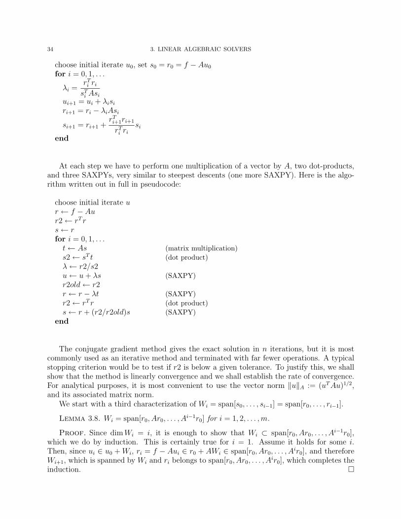
At each step we have to perform one multiplication of a vector by A, two dot-products,and three SAXPYs, very similar to steepest descents (one more SAXPY). Here is the algo-rithm written out in full in pseudocode:
choose initial iterate ur ← f − Aur2← rT rs← rfor i = 0, 1, . . .t← As (matrix multiplication)s2← sT t (dot product)λ← r2/s2u← u+ λs (SAXPY)r2old← r2r ← r − λt (SAXPY)r2← rT r (dot product)s← r + (r2/r2old)s (SAXPY)
end
The conjugate gradient method gives the exact solution in n iterations, but it is mostcommonly used as an iterative method and terminated with far fewer operations. A typicalstopping criterion would be to test if r2 is below a given tolerance. To justify this, we shallshow that the method is linearly convergence and we shall establish the rate of convergence.For analytical purposes, it is most convenient to use the vector norm ‖u‖A := (uTAu)1/2,and its associated matrix norm.
We start with a third characterization of Wi = span[s0, . . . , si−1] = span[r0, . . . , ri−1].
Lemma 3.8. Wi = span[r0, Ar0, . . . , Ai−1r0] for i = 1, 2, . . . ,m.
Proof. Since dimWi = i, it is enough to show that Wi ⊂ span[r0, Ar0, . . . , Ai−1r0],
which we do by induction. This is certainly true for i = 1. Assume it holds for some i.Then, since ui ∈ u0 + Wi, ri = f − Aui ∈ r0 + AWi ∈ span[r0, Ar0, . . . , A
ir0], and thereforeWi+1, which is spanned by Wi and ri belongs to span[r0, Ar0, . . . , A
ir0], which completes theinduction.

2. THE CONJUGATE GRADIENT METHOD 35
The space span[r0, Ar0, . . . , Ai−1r0] is called the Krylov space generated by the matrix A
and the vector r0. Note that we have as well
Wi = span[r0, Ar0, . . . , Ai−1r0] = p(A)r0 | p ∈ Pi−1 = q(A)(u− u0) | q ∈ Pi, q(0) = 0 .
Here Pi denotes the space of polynomials of degree at most i. Since ri is l2-orthogonal toWi, u− ui is A-orthogonal to Wi, so
‖u− ui‖A = infw∈Wi
‖u− ui + w‖A.
Since ui − u0 ∈ Wi,infw∈Wi
‖u− ui + w‖A = infw∈Wi
‖u− u0 + w‖A.
Combining the last three equations, we get
‖u− ui‖A = infq∈Piq(0)=0
‖u− u0 + q(A)(u− u0)‖A = infp∈Pip(0)=1
‖p(A)(u− u0)‖A.
Applying the obvious bound ‖p(A)(u−u0)‖A ≤ ‖p(A)‖A‖u−u0‖A we see that we can obtainan error estimate for the conjugate gradient method by estimating
K = infp∈Pip(0)=1
‖p(A)‖A.
Now if 0 < ρ1 < · · · < ρn are the eigenvalues of A, then the eigenvalues of p(A) are p(ρj),j = 1, . . . , n, and ‖p(A)‖A = maxj |p(ρj)|. Thus1
K = infp∈Pip(0)=1
maxj|p(ρj)| ≤ inf
p∈Pip(0)=1
maxρ1≤ρ≤ρn
|p(ρ)|.
The final infimum can be calculated explicitly, as will be explained below. Namely, for any0 < a < b, and integer n > 0,
(3.6) minp∈Pn
p(0)=1
maxx∈[a,b]
|p(x)| = 2(√b/a+1√b/a−1
)n+
(√b/a−1√b/a+1
)n .This gives
K ≤ 2(√κ+1√κ−1
)i+(√
κ−1√κ+1
)i ≤ 2
(√κ− 1√κ+ 1
)i,
where κ = ρn/ρ1 is the condition number of A. (To get the right-hand side, we suppressedthe second term in the denominator of the left-hand side, which is less than 1 and tends tozero with i, and kept only the first term, which is greater than 1 and tends to infinity withi.) We have thus proven that
‖u− ui‖A ≤ 2
(√κ− 1√κ+ 1
)i‖u− u0‖A,
1Here we bound maxj |p(ρj)| by maxρ1≤ρ≤ρn|p(ρ)| simply because we can minimize the latter quantity
explicitly. However this does not necessarily lead to the best possible estimate, and the conjugate gradientmethod is often observed to converge faster than the result derived here. Better bounds can sometimes beobtained by taking into account the distribution of the spectrum of A, rather than just its minimum andmaximum.

36 3. LINEAR ALGEBRAIC SOLVERS
which is linear convergence with rate
r =
√κ− 1√κ+ 1
.
Note that r ∼ 1 − 2/√κ for large κ. So the convergence deteriorates when the condition
number is large. However, this is still a notable improvement over the classical iterations.For the discrete Laplacian, where κ = O(h−2), the convergence rate is bounded by 1 − ch,not 1− ch2.
The above analysis yields a convergence estimate for the method of steepest descent aswell. Indeed, the first step of conjugate gradients coincides with steepest descents, and so,for steepest descents,
‖u− u1‖A ≤2
√κ+1√κ−1
+√κ−1√κ+1
‖u− u0‖A =κ− 1
κ+ 1‖u− u0‖A.
Of course, the same result holds if we replace u0 by ui and u1 by ui+1. Thus steepestdescents converges linearly, with rate (κ− 1)/(κ+ 1) (just like Richardson iteration with theoptimal parameter). Notice that the estimates indicate that a large value of κ will slow theconvergence of both steepest descents and conjugate gradients, but, since the dependencefor conjugate gradients is on
√κ rather than κ, the convergence of conjugate gradients will
usually be much faster.The figure shows a plot of the norm of the residual versus the number of iterations for
the conjugate gradient method and the method of steepest descents applied to a matrixof size 233 arising from a finite element simulation. The matrix is irregular, but sparse(averaging about 6 nonzero elements per row), and has a condition number of about 1, 400.A logarithmic scale is used on the y-axis so the near linearity of the graph reflects linearconvergence behavior. For conjugate gradients, the observed rate of linear convergence isbetween .7 and .8, and it takes 80 iterations to reduce the initial residual by a factor ofabout 106. The convergence of steepest descents is too slow to be useful: in 400 iterationsthe residual is not even reduced by a factor of 2.
Remark. There are a variety of conjugate-gradient-like iterative methods that apply tomatrix problems Au = f where A is either indefinite, non-symmetric, or both. Many sharethe idea of approximation of the solution in a Krylov space.
Our analysis of conjugate gradients and steepest descents depended on the explicit so-lution of the minimization problem given in (3.6). Here we outline the proof of this result,leaving the details as an exercise.
The Chebyshev polynomials are defined by the recursion
T0(x) = 1, T1(x) = x, Tn+1(x) = 2xTn(x)− Tn−1(x) for n = 1, 2, . . .,
so Tn is a polynomial of degree n. From this follows two explicit formulas for Tn:
Tn(x) = cos(n arccosx), Tn(x) =1
2[(x+
√x2 − 1)n + (x−
√x2 − 1)n],
with the first equation valid for |x| ≤ 1 and the second valid for |x| ≥ 1.The polynomial Tn satisfies |Tn(x)| ≤ 1 on [−1, 1] with equality holding for n+ 1 distinct
numbers in [−1, 1]. This can be used to establish the following: for any α < 1, there does not

2. THE CONJUGATE GRADIENT METHOD 37
Figure 3.3. Convergence of conjugate gradients for solving a finite elementsystem of size 233. On the left 300 iterations are shown, on the right the first50. Steepest descents is shown for comparison.
0 50 100 150 200 25010
−40
10−30
10−20
10−10
100
1010
iterations
norm
of r
esid
ual
CG
SD
0 10 20 30 40 5010
−2
10−1
100
101
102
iterationsno
rm o
f res
idua
l
Figure 3.4. The quintic polynomial equal to 1 at 0 with the smallest L∞
norm on [2, 10]. This is a scaled Chebyshev polynomial, and so the norm canbe computed exactly.
0 2 4 6 8 10 12−0.2
0
0.2
0.4
0.6
0.8
1
2 4 6 8 10−0.05
−0.025
0
0.025
0.05
0.075
0.1
exist any polynomial q ∈ Pn with q(α) = Tn(α) and |q(x)| < 1 on [−1, 1]. In other words,Tn minimizes of maxx∈[−1,1] |p(x)| over all polynomials in Pn which take the value Tn(α) atα.
Scaling this result we find that
p(x) =
[Tn
(−b+ a
b− a
)]−1
Tn
(2x− b− ab− a
)solves the minimization problem (3.6) and gives the minimum value claimed. This polyno-mial is plotted for n = 5, a = 2, b = 10 in Figure 3.4.

38 3. LINEAR ALGEBRAIC SOLVERS
2.3. Preconditioning. The idea is we choose a matrix M ≈ A such that the systemMz = c is relatively easy to solve. We then consider the preconditioned system M−1Ax =M−1b. The new matrix M−1A is SPD with respect to the M inner product, and we solvethe preconditioned system using conjugate gradients but using the M -inner product in placeof the l2-inner product. Thus to obtain the preconditioned conjugate gradient algorithm, orPCG, we substitute M−1A for A everywhere and change expressions of the form xTy intoxTMy. Note that the A-inner product xTAy remains invariant under these two changes.Thus we obtain the algorithm:
choose initial iterate u0, set s0 = r0 = M−1f −M−1Au0
for i = 0, 1, . . .
λi =rTi MrisTi Asi
ui+1 = ui + λisiri+1 = ri − λiM−1Asi
si+1 = ri+1 +rTi+1Mri+1
rTi Mrisi
end
Note that term sTi Asi arises as the M -inner product of si with M−1Asi. The quantityri is the residual in the preconditioned equation, which is related to the regular residual,ri = f − Aui by ri = Mri. Writing PCG in terms of ri rather than ri we get
choose initial iterate u0, set r0 = f − Au0, s0 = M−1r0
for i = 0, 1, . . .
λi =rTi M
−1risTi Asi
ui+1 = ui + λisiri+1 = ri − λiAsisi+1 = M−1ri+1 +
rTi+1M−1ri+1
rTi M−1ri
si
end
Thus we need to compute M−1ri at each iteration. Otherwise the work is essentially thesame as for ordinary conjugate gradients. Since the algorithm is just conjugate gradients forthe preconditioned equation we immediately have an error estimate:
‖ui − u‖A ≤ 2
(√κ− 1√κ+ 1
)i‖u0 − u‖A,
where κ now is the ratio of the largest to the least eigenvalue of M−1A. To the extent thatM approximates A, this ratio will be close to 1 and so the algorithm will converge quickly.
The matrix M is called the preconditioner. A good preconditioner should have two prop-erties. First, it must be substantially easier to solve systems with the matrix M than with

2. THE CONJUGATE GRADIENT METHOD 39
the original matrix A, since we will have to solve such a system at each step of the precon-ditioned conjugate gradient algorithm. Second, the matrix M−1A should be substantiallybetter conditioned than A, so that PCG converges faster than ordinary CG. In short, Mshould be near A, but much easier to invert. Note that these conditions are similar to thosewe look for in defining a classical iteration via residual correction. If ui+1 = ui +B(f −Aui)is an iterative method for which B is SPD, then we might use M = B−1 as a preconditioner.For example, the Jacobi method suggests taking M to be the diagonal matrix with the samediagonal entries as A. When we compute M−1ri in the preconditioned conjugate gradientalgorithm, we are simply applying one Jacobi iteration. Similarly we could use symmetricGauss-Seidel to get a preconditioner.
In fact, we can show that conjugate gradients preconditioned by some SPD approximateinverse always converges faster than the corresponding classical iterative method. For if λ isan eigenvalue of BA, then −ρ ≤ 1− λ ≤ ρ where ρ is the spectral radius of I −BA, and so
λmin(BA) ≥ 1− ρ, λmax(BA) ≤ 1 + ρ, κ(BA) ≤ 1 + ρ
1− ρ.
Thus the rate of convergence for the PCG method is at most√κ(BA)− 1√κ(BA) + 1
≤
√1+ρ1−ρ − 1√1+ρ1−ρ + 1
=1−
√1− ρ2
ρ.
The last quantity is strictly less than ρ for all ρ ∈ (0, 1). (For ρ small it is about ρ/2, whilefor the important case of ρ ≈ 1 − ε with ε small, it is approximately 1 −
√2ε.) Thus the
rate of convergence of PCG with B as a preconditioner is better than that of the classicaliteration with B as approximate inverse.
Diagonal (Jacobi) preconditioning is often inadequate (in the case of the 5-point Lapla-cian it accomplishes nothing, since the diagonal is constant). Symmetric Gauss-Seidel issomewhat better, but often insufficient as well. A third possibility which is often appliedwhen A is sparse is to determine M via the incomplete Cholesky factorization. This meansthat a triangular matrix L is computed by the Cholesky algorithm applied to A, except thatno fill-in is allowed: only the non-zero elements of A are altered, and the zero elements leftuntouched. One then takes M = LLT , and, so M−1 is easy to apply. Yet, other precondi-tioners take into account the source of the matrix problem. For example, if a matrix arisesfrom the discretization of a complex partial differential equation, we might precondition itby the discretization matrix for a simpler related differential equation (if that lead to a linearsystems which is easier to solve). In fact the derivation of good preconditioners for importantclasses of linear systems remain a very active research area.
We close with numerical results for preconditioned conjugate gradients with both the di-agonal preconditioner and incomplete Cholesky factorization as preconditioner. In Figure 3.5we reproduce the results shown in Figure 3.3, together with these preconditioned iterations.By fitting the log of the norm of the residual to a linear polynomial, we can compute theobserved rates of linear convergence. They are The preconditioned methods are much more
steepest descents 0.997 PCG (diag.) 0.529conjugate gradients 0.725 PCG (IC) 0.228

40 3. LINEAR ALGEBRAIC SOLVERS
effective. Diagonal preconditioning reduces the number of iterations needed by conjugategradients to reduce the initial error by a factor of 10−6 from 80 to 44. Incomplete Choleskypreconditioning reduces further to 18 iterations.
Figure 3.5. Convergence of conjugate gradients for solving a finite elementsystem of size 233, unpreconditioned, diagonally preconditioned, and precon-ditioned by incomplete Cholesky factorization. Steepest descents is shown aswell. On the left 300 iterations are shown, on the right the first 50.
0 50 100 150 200 25010
−200
10−150
10−100
10−50
100
1050
iterations
norm
of r
esid
ual
CG
SD
PCG (diag)
PCG (IC)
0 10 20 30 40 5010
−30
10−20
10−10
100
1010
iterations
norm
of r
esid
ual
CGPCG (diag)
SD
PCG (IC)
3. Multigrid methods
Figure 3.6 shows the result of solving a discrete system of the form −∆huh = f using theGauss–Seidel iteration. We have take h = 64, and chosen a smooth right-hand side vectorf which results in the vector uh which is shown in the first plot. The initial iterate u0,which is shown in the second plot, was chosen at random, and then the iterates u1, u2, u10,u50, and u500 are shown in the subsequent plots. In Figure 3.7, the maximum norm error‖uh − ui‖/‖uh‖ is plotted for i = 0, 1, . . . , 50.
These numerical experiments illustrate the following qualitative properties, which aretypical of the Gauss–Seidel iteration applied to matrices arising from the discretization ofelliptic PDEs.
• If we start with a random error, the norm of the error will be reduced fairly quicklyfor the first few iterations, but the error reduction occurs much more slowly afterthat.• After several iterations the error is much smoother, but not much smaller, than
initially. Otherwise put, the highly oscillatory modes of the error are suppressedmuch more quickly by the iteration than the low frequency modes.
The first observation is valid for all the methods we have studied: Richardson, Jacobi,damped Jacobi, and Gauss–Seidel. The second obervation—that Gauss–Seidel iterationsmooths the error—is shared damped Jacobi with α < 1, but not by Jacobi itself.
If we take the Richardson method with ω = 1/λmax(A) for the operator A = −D2h,
it is very easy to see how the smoothing property comes about. The initial error can beexpanded in terms of the eigenfunctions of A: e0 =
∑nm=1 ci sinmπx. The mth component

3. MULTIGRID METHODS 41
Figure 3.6. Iterative solution to −∆huh = f , h = 1/64, using Gauss–Seidel.The random initial iterate is rapidly smoothed, but approaches the solutionuh only very slowly.
exact solution initial iterate
iterate 1 iterate 2
iterate 10 iterate 50

42 3. LINEAR ALGEBRAIC SOLVERS
Figure 3.7. Error in the Gauss–Seidel iterates 0 through 50 in l∞ (•).
in this expansion is multiplied by 1 − λm/λmax = 1 − λm/λn at each iteration. Thus thehigh frequency components, m ≈ n, are multiplied by something near to 0 at each iteration,and so are damped very quickly. Even the intermediate eigenvalues, λm ≈ λn/2 are dampedreasonably quickly (by a factor of about 1/2 at each iteration). But the low frequency modes,for which λm λn, decrease very slowly.
This also explains the first observation, that the norm of the error decreases quicklyat first, and then more slowly. The norm of the error has contributions from all modespresent in the initial error. Those associated to the higher frequency modes disappear in afew iterations, bringing the error down by a significant fraction. But after that the error isdominated by the low frequency modes, and so decays very slowly.
The same analysis applies to damped Jacobi with positive damping, and shows thatundamped Jacobi doesn’t have the smoothing property: the mth mode is multiplied byabout 1 − 2λm/λn, and so convergence is very slow for low frequency modes and also thehighest frequency modes λm ≈ λn. For the intermediate modes, λm ≈ λn/2, convergence isvery fast.
Establishing the smoothing property for Gauss–Seidel is more complicated, since theeigenfunctions of the Gauss–Seidel iteration don’t coincide with those of A even for A = −D2
h.However both numerical study and careful analysis show that Gauss–Seidel does indeed havethe smoothing property for discretized elliptic operators.
The idea behind the multigrid method is to create an iterative method which reduces allcomponents of the residual quickly by putting together two steps. First it applies the approx-imate inverse from Gauss–Seidel or another classical iterative method with the smoothingproperty to the residual. This greatly reduces the high frequency components of the resid-ual, but barely reduces the low frequency components. The new residual, being relativelysmooth, can then be accurately approximated on a coarser mesh. So, for the second step,the residual is (somehow) transferred to a coarser mesh, and the equation solved there, thus

3. MULTIGRID METHODS 43
reducing the low frequency components. On the coarser mesh, it is of course less expensiveto solve. For simplicity, we assume for now that an exact solver is used on the coarse mesh.Finally this coarse mesh solution to the residual problem is somehow transferred back to thefine mesh where it can be added back to our smoothed approximation.
Thus we have motivated the following rough outline of an algorithm:
(1) Starting from an initial guess u0 apply a fine mesh smoothing iteration to get animproved approximation u.
(2) Transfer the residual in u to a coarser mesh, solve a coarse mesh version of theproblem there, transfer the solution back to the fine mesh, and add it back to u toget ¯u.
Taking ¯u for u1 and thus have described an iteration to get from u0 to u1 (which we canthen apply again to get from u1 to u2, and so on). In fact it is much more common to alsoapply a fine mesh smoothing at the end of the iteration, i.e., to add a third step:
3. Starting from ¯u apply the smoothing iteration to get an improved approximation ¯u.
The point of including the third step is that it leads to a multigrid iteration which is sym-metric, which is often advantageous (e.g., the iteration can be used as a preconditioner forconjugate gradients). If the approximation inverse B used for the first smoothing step is notsymmetric, we need to apply BT (which is also an approximate inverse, since A is symmetric)to obtain a symmetric iteration.
We have just described a two-grid iteration. The true multigrid method will involve notjust the original mesh and one coarser mesh, but a whole sequence of meshes. However, oncewe understand the two-grid iteration, the multigrid iteration will follow easily.
To make the two-grid method more precise we need to explain step 2 more fully, namely(a) how do we transfer the residual from the fine mesh to the coarse mesh?; (b) what problemdo we solve on the coarse mesh?; and (c) how do we transfer the solution of that problemfrom the coarse mesh to the fine mesh? For simplicity, we suppose that N = 1/h is evenand that we are interested in solving Ahu = f where A = −D2
h. Let H = 2h = (N/2)−1.We will use the mesh of size H as our coarse mesh. The first step of our multigrid iterationis then just
u = u0 +Bh(f − Ahu0),
where Bh is just the approximate inverse of Ah from Gauss–Seidel or some other smoothingiteration. The resulting residual is f − Ahu. This is a function on the fine mesh pointsh, 2h, . . . , (N − 1)h, and a natural way to transfer it to the coarse mesh is restrict it to theeven grid points 2h, 4h, . . . , (N −2)h = H, 2H, . . . , (N/2−1)H, which are exactly the coarsemesh grid points. Denoting this restriction operator from fine grid to coarse grid functions(i.e., from RN−1 → RN/2−1) by PH , we then solve AHeH = PH(f − Ahuh) where, of course,AH = −D2
H is the 3-point difference operator on the coarse mesh. To transfer the solution eH ,a coarse grid function, to the fine grid, we need a prolongation operator QH : RN/2−1 → RN−1.It is natural to set QHeH(jh) = eH(jh) if j is even. But what about when j is odd: howshould we define QHeH at the midpoint of two adjacent coarse mesh points? A naturalchoice, which is simple to implement, is QHeH(jh) = [eH((j − 1)h) + e((j + 1)h)]/2. Withthese two operators second step is
¯u = u+QHA−1H PH(f − Ahu).

44 3. LINEAR ALGEBRAIC SOLVERS
And then final post-smoothing step is
¯u = ¯u+BTh (f − Ah ¯u).
Actually this does not give a symmetric iteration. To obtain symmetry we need Qh = cP TH
and that is not the case for the grid transfer operators we defined. We have
(3.7) QH =
1/2 0 0 0 · · · 01 0 0 0 · · · 0
1/2 1/2 0 0 · · · 00 1 0 0 · · · 00 1/2 1/2 0 · · · 0...
......
.... . .
...0 0 0 0 · · · 1/2
,
but PH as we described it, consists only of 0’s and 1’s. Therefore one commonly takes adifferent choice for PH , namely PH = (1/2)QT
H . This means that the transferred coarse gridfunction doesn’t just take the value of the corresponding fine grid function at the coarse gridpoint, but rather uses a weighted average of the fine grid function’s values at the point inquestion and the fine grid points to the left and right (with weights 1/4, 1/2, 1/4). Withthis choice, QHAhPH is symmetric; in fact, QHAhPH = AH . This is a useful formula. Foroperators other than the Ah = −D2
h, we can use the same intergrid transfer operators,namely QH given by (3.7) and PH = (1/2)QT
H , and then define the coarse grid operator byAH = QHAhPH .
Remark. In a finite element context, the situation is simpler. If the fine mesh is arefinement of the coarse mesh, then a coarse mesh function is already a fine mesh function.Therefore, the operator QH can be taken simply to be the inclusion operator of the coarsemesh space into the fine mesh space. The residual in u0 ∈ Sh is most naturally viewed asa functional on Sh: v 7→ (f, v) − B(u0, v). It is then natural to transfer the residual to thecoarse mesh simply by restricting the test function v to SH . This operation STh → STH isexactly the adjoint of the inclusion operator SH → Sh. Thus the second step, solving thecoarse mesh problem for the restricted residual is obvious in the finite element case: we findeH ∈ SH such that
B(eH , v) = (f, v)−B(u, v), v ∈ SH ,
and then we set ¯u = u+ eH ∈ Sh.
Returning to the case of finite differences we have arrived at the following two-griditerative method to solve Ahuh = fh.

3. MULTIGRID METHODS 45
uh = twogrid(h,Ah, fh, u0)input: h, mesh size (h = 1/n with n even)
Ah, operator on mesh functionsfh, mesh function (right-hand side)u0, mesh function (initial iterate)
output: uh, mesh function (approximate solution)
for i = 0, 1, . . . until satisfied1. presmoothing: u = ui +Bh(fh − Ahui)2. coarse grid correction:
2.1. residual computation: rh = fh − Ahu2.2. restriction: H = 2h, rH = PHrh, AH = PHAhQH
2.3. coarse mesh solve: solve AHeH = rH2.4. prolongation: eh = QHeH2.5. correction: ¯u = u+ eh
3. postsmoothing: uh ← ui+1 = ¯u+BTh (fh − Ah ¯u)
end
Algorithm 3.1: Two-grid iteration for approximately solving Ahuh = fh.
In the smoothing steps, the matrix Bh could be, for example, (D − L)−1 where D isdiagonal, L strictly lower triangular, and Ah = D − L− LT . This would be a Gauss–Seidelsmoother, but there are other possibilities as well. Besides these steps, the major work is inthe coarse mesh solve. To obtain a more efficient algorithm, we may also solve on the coarsemesh using a two-grid iteration, and so involving an even coarser grid. In the followingmultigrid algorithm, we apply this idea recursively, using multigrid to solve at each meshlevel, until we get to a sufficiently coarse mesh, h = 1/2, at which point we do an exact solve(with a 1× 1 matrix!).

46 3. LINEAR ALGEBRAIC SOLVERS
uh = multigrid(h,Ah, fh, u0)input: h, mesh size (h = 1/n with n a power of 2)
Ah, operator on mesh functionsfh, mesh function (right-hand side)u0, mesh function (initial iterate)
output: uh, mesh function (approximate solution)
if h = 1/2 thenuh = A−1
h fhelse
for i = 0, 1, . . . until satisfied1. presmoothing: u = ui +Bh(f − Ahui)2. coarse grid correction:
2.1. residual computation: rh = fh − Ahu2.2. restriction: H = 2h, rH = PHrh, AH = PHAhQH
2.3. coarse mesh solve: eH = multigrid(H,AH , rH , 0)2.4. prolongation: eh = QHeH2.5. correction: ¯u = u+ eh
3. postsmoothing: uh ← ui+1 = ¯u+BTh (f − Ah ¯u)
endend if
Algorithm 3.2: Multigrid iteration for approximately solving Ahuh = f .
Figure 3.8 shows 5 iterations of this multigrid algorithm for solving the system −∆huh =f , h = 1/64, considered at the beginning of this section, starting from a random initialguess (we would get even better results starting from a zero initial guess). Compare withFigure 3.6. The fast convergence of the multigrid algorithm is remarkable. Indeed, forthe multigrid method discussed here it is possible to show that the iteration is linearlyconvergent with a rate independent of the mesh size (in this example, it is roughly 0.2).This means that the number of iterations needed to obtain a desired accuracy remainsbounded independent of h. It is also easy to count the number of operations per iteration.Each iteration involves two applications of the smoothing iteration, plus computation ofthe residual, restriction, prolongation, and correction on the finest mesh level. All thoseprocedures cost O(n) operations. But then, during the coarse grid solve, the same proceduresare applied on the grid of size 2h, incurring an additional cost of O(n/2). Via the recursionthe work will be incurred for each mesh size h, 2h, 4h, . . .. Thus the total work per iterationwill be O(n + n/2 + n/4 + . . . + 1) = O(n) (since the geometric series sums to 2n). Thusthe total work to obtain the solution of the discrete system to any desired accuracy is itselfO(n), i.e., optimal.

3. MULTIGRID METHODS 47
Figure 3.8. Iterative solution to −∆huh = f , h = 1/64, using multigrid.
initial iterate iterate 1
iterate 2 iterate 3
iterate 4 iterate 5

CHAPTER 4
Finite element methods for elliptic equations
1. Weak and variational formulations
Model PDE: − div a gradu+ cu = f in Ω
Here Ω is a bounded domain in Rn; 0 < a ≤ a(x) ≤ a, 0 ≤ c(x) ≤ c
First consider the homogeneous Dirichlet BC: u = 0 on ∂Ω.
Assuming that a ∈ C1(Ω), c ∈ C(Ω), u ∈ C2(Ω) satisfies the PDE and BC (a strongsolution), then it also satisfies the weak formulation:
Find u ∈ H1(Ω) such that∫(a gradu · grad v + cuv) =
∫fv, v ∈ H1(Ω),
A solution of the weak formulation need not belong to C2(Ω), but if it does, then it is astrong solution.
The variational formulation is completely equivalent to the weak formulation
u = argminv∈H1(Ω)
∫Ω
[1
2(a grad v · grad v + cv2)− fv]
Extensions: Neumann BC, Robin BC, mixed BC, inhomogeneous Dirichlet BC. Firstorder term to the PDE (then the problem is not symmetric and there is no variationalformulation, but weak formulation is fine).
All these problems can be put in the weak form: Find u ∈ V such that
(4.1) b(u, v) = F (v), v ∈ V,
where V is a Hilbert space (H1 or H1), b : V × V → R is a bilinear form, F : V → R isa linear form. (The inhomogeneous Dirichlet problem takes this form if we solve for u− ugwhere ug is a function satisfying the inhomogeneous Dirichlet BC ug = g on ∂Ω.) Forsymmetric problems (no first order term), the bilinear form b is symmetric, and the weakform is equivalent to the variational form:
u = argminv∈V
[1
2b(v, v)− F (v)].
49

50 4. FINITE ELEMENT METHODS FOR ELLIPTIC EQUATIONS
2. Galerkin method and finite elements
Let Vh be a finite dimensional subspace of V . If we replace the V in the weak formulationwith Vh we get a discrete problem: Find uh ∈ Vh such that
(4.2) b(uh, v) = F (v), v ∈ Vh.
This is called the Galerkin method. For symmetric problems it is equivalent to the Rayleigh–Ritz method, which replaces V by Vh in the variational formulation:
uh = argminv∈Vh
[1
2b(v, v)− F (v)].
The Galerkin solution can be reduced to a set of n linear equations in n unknowns wheren = dimVh by choosing a basis. Adopting terminology from elasticity, the matrix is calledthe stiffness matrix and the right hand side is the load vector.
Comparing (4.1) and (4.2), we find that the error in the Galerkin method u−uh satisfies
(4.3) b(u− uh, v) = 0, v ∈ Vh.
This relation, known as Galerkin orthogonality, is key to the analysis of Galerkin methods.To define a simple finite element method, we suppose that Ω is a polygon in R2 and let Th
be a simplicial decomposition of Ω (covering of Ω by closed triangles so that the intersectionof any two distinct elements of Th is either empty or a common edge or vertex. Let
M10 (Th) = v ∈ C(Ω) |V |T ∈ P1(T )∀T ∈ Th = v ∈ H1(Ω) |V |T ∈ P1(T )∀T ∈ Th ,
and M10 (Th) = H1(Ω) ∩M1
0 (Th). The P1 finite element method for the Dirichlet problem is
the Galerkin method with Vh = M10 (Th).
We can use the Lagrange (hat function) basis for Vh to ensure that (1) the matrix issparse, and (2) the integrals entering into the stiffness matrix and load vector are easy tocompute.
Figure 4.1. A hat function basis element for M10 (Th).
In the special case where Ω is the unit square, and Th is obtained from a uniform m×mpartition into subsquares, each bissected by its SW-NE diagonal (so n = (m − 1)2), theresulting stiffness matrix is exactly the same as the matrix of the 5-point Laplacian.
3. LAGRANGE FINITE ELEMENTS 51
3. Lagrange finite elements
This section is written mostly for 2D, although extending to n dimensions is straightfor-ward.
A finite element space is a space of piecewise polynomials with respect to a given trian-gulation (simplicial decomposition) Th, but not just any space of piecewise polynomials. Itis constructed by specifying the following things for each T ∈ Th:
• Shape functions : a finite dimensional space V (T ) consisting of polynomial functionson T .• Degrees of freedom: a finite set of linear functionals V (T )→ R which are unisolvent
on V (T ). This means that real values can be assigned arbitrarily to each DOF, andthese determine one and only one element of V (T ). In other words, the DOF forma basis for the dual space of V (T ).
We further assume that each degree of freedom on T is associated to a subsimplex of T , i.e.,to a vertex, an edge, or T itself (in 2D). Moreover, if a subsimplex is shared by two differenttriangles in T1 and T2 in Th, the DOFs for T1 and T2 associated to the subsimplex are in1-to-1 correspondence.
When all this is specified, the assembled finite element space is defined as all functionsv ∈ L2(Ω) such that
• v|T ∈ V (T ) for all T ∈ Th• The DOFs are single-valued in the sense that whenever q is a subsimplex shared byT1 and T2, then the corresponding DOFs on applied to v|T1 and v|T2 take on thesame value.
Note that we do not specify the interelement continuity explicitly. It is determined by thefact that the shared DOFs are single-valued.
The reason for this definition is that it is easy to construct and compute with piecewisepolynomial spaces defined in this way. First of all, we immediately obtain a set of globaldegrees of freedom, by considering all the degrees of freedom associated with all the sub-simplices of the triangulation. An element of the FE space is uniquely determined by anarbitrary assignment of values to the global degrees of freedom. Thus the dimension of theFE space is the sum over the subsimplices of the number of degrees of freedom associatedto the subsimplex. A basis for the FE space is obtained by setting one of the global DOFsto 1 and all the rest to zero. The resulting basis function is supported in the union of thetriangles which contain the subsimplex. Thus we have a local basis (small supports), andwill obtain a sparse stiffness matrix.
The simplest example is the P1 element, or Lagrange element of degree 1, discussed above.Then the shape functions are simply the linear polynomials: V (T ) = P1(T ) (dimensionequals 3 is 2D). The degrees of freedom on T are the evaluation functionals associated tothe 3 vertices. These DOFs are certainly unisolvent: a linear function in 2D is determinedby its value at any 3 non-colinear points. Clearly any continuous piecewise linear functionbelongs to the FE space, since it can be specified by assigning its vertex values. Conversely,if v is an element of the assembed FE space and two triangles T1 and T2 share a commonedge e, then v|T1 and v|T2 must agree on all of e, since on e they are both linear functions,and they agree at the two end points of e (a linear function in 1D is determined by its valueat any 2 distinct points). This shows that the assembled FE space consists precisely of the

52 4. FINITE ELEMENT METHODS FOR ELLIPTIC EQUATIONS
continuous piecewise linears. The global degrees of freedom are the vertex values, and thecorresponding local basis consists of the hat functions.
For the Lagrange element of degree 2, the shape functions are V (T ) = P2(T ). There isone DOF associated to each vertex (evaluation at the vertex), and one associated to eachedge (evaluation at the midpoint of the edge). Let us check unisolvence. Since dimV (T ) = 6and there are 6 DOFs on T , we must show that if all 6 DOFs vanish for some v ∈ V (T ),then v ≡ 0. For this choose a numbering of the vertices of T , and let λi ∈ P1(R2), i = 1, 2, 3,denote the linear function that is 1 on the ith vertex and which vanishes on the oppositeedge, e of T . Thus the equation λi = 0 is the equation of the line through the edge e. Sincev vanishes at the two endpoints and the midpoint of e, v|e vanishes (a quadratic in 1D whichvanishes at 3 points is zero). Therefore v is divisible by the linear polynomial λi, for eachi. Thus v is a multiple of λ1λ2λ3. But v is quadratic and this product is cubic, so the onlypossibility is that v ≡ 0. It is easy to check that the assembled space is exactly the spaceM2
0 (Th) of continuous piecewise quadratic functions. There is one basis function associatedto each vertex and one to each edge.
Figure 4.2. Basis functions for M20 (Th).
Note: the linear functions λi are the barycentric coordinate functions on T . They satisfyλ1 + λ2 + λ3 ≡ 1.
Higher degree Lagrange elements are defined similarly. V (T ) = Pr(T ). dimV (T ) =(r+ 1)(r+ 2)/2. There is 1 DOF at each vertex, r− 1 on each edge, and (r− 2)(r− 1)/2 ineach triangle. Note that 3× 1 + 3× (r− 1) + (r− 2)(r− 1)/2 = (r+ 1)(r+ 2)/2. The DOFs

4. COERCIVITY, INF-SUP CONDITION, AND WELL-POSEDNESS 53
are the evaluation functionals at the points with barycentric coordinates all of the form i/rwith 0 ≤ i ≤ r and integer.
Additional material covered here, notes not available: Data structures for triangulations,the finite element assembly process (loops over elements).
Other finite element spaces. Cubic Hermite finite elements. Shape functions are P3(T )for a triangle T . Three DOFs for each vertex v: u 7→ u(v), u 7→ (∂u/∂x)(v), u 7→ (∂u/∂y)(v);and one DOF associated to the interior u 7→
∫Tv (alternatively, evaluation at the barycenter).
Proof of unisolvence. Note that the assembled finite element space belongs to C0 and H1,but not to C1 and H2.
Figure 4.3. Cubic Hermite element.
Quintic Hermite finite elements (Argyris elements). Shape functions are P5(T ) for atriangle T . Six DOFs for each vertex v: evaluation of u, both 1st partials, and all three 2ndpartials of u at v. One DOF for each edge: evaluation of ∂u/∂n at midpoint. Unisolvent,H2.
Figure 4.4. Quintic Hermite element.
4. Coercivity, inf-sup condition, and well-posedness
First we consider this in an abstract framework, in which we are given a Hilbert spaceV , a bounded bilinear form b : V × V → R and a bounded linear form F : V → R, and theproblem we wish to solve is
(4.4) b(u, v) = F (v), v ∈ V.We will analyze the Galerkin method using the ideas of stability and consistency we intro-duced in Chapter 2, § 1.2. Recall that there we studied a problem of the form find u ∈ Xsuch that Lu = f where L mapped the vector space X where the solution was sought to

54 4. FINITE ELEMENT METHODS FOR ELLIPTIC EQUATIONS
the vector space Y where the data f belonged. For the problem (4.4), the solution spaceX = V , and the data space Y = V ∗, the dual space of V . The linear operator L is simplygiven by
Lw(v) = b(w, v) w, v ∈ V.So the problem (4.4) is simply: given F ∈ V ∗ find u ∈ V such that Lu = F .
First of all, before turning to discretization, we consider the well-posedness of this prob-lem. We have already assumed that the bilinear form b is bounded, i.e., there exists aconstant M such that
|b(w, v)| ≤M‖w‖‖v‖, w, v ∈ V,where, of course, the norm is the V norm. This implies that the operator L : V → V ∗ is abounded linear operator (with the same bound).
We will now consider hypotheses on the bilinear form b that ensure that the problem(4.4) is well-posed. We will consider three cases, in increasing generality.
4.1. The symmetric coercive case. First we assume that the bilinear form b is sym-metric (b(w, v) = b(v, w)) and coercive, which means that there exists a constant γ > 0, suchthat
b(v, v) ≥ γ‖v‖2, v ∈ V.In this case b(w, v) is an inner product on V , and the associated norm is equivalent to theV norm:
γ‖v‖2V ≤ b(v, v) ≤M‖v‖2
V .
Thus V is a Hilbert space when endowed with the b inner product, and the Riesz Represen-tation Theorem gives that for all F ∈ V ∗ there exists a unique u ∈ V such that
b(u, v) = F (v), v ∈ V,
i.e., (4.4) has a unique solution for any data, and L−1 : V ∗ → V is well-defined. Takingv = u and using the coercivity condition we immediately have γ‖u‖2
V ≤ F (u) ≤ ‖F‖V ∗‖u‖V ,so ‖u‖V ≤ γ−1‖F‖V , i.e., ‖L−1‖L(V ∗,V ) ≤ γ−1.
In short, well-posedness is an immediate consequence of the Riesz Representation Theo-rem in the symmetric coercive case.
As a simple example of the utility of this result, let us consider the Neumann problem
− div a gradu+ cu = f in Ω, a∂u
∂n= 0 on ∂Ω
where 0 < a ≤ a(x) ≤ a, 0 < c ≤ c(x) ≤ c. The weak formulation is: Find u ∈ V such that
b(u, v) = F (v), v ∈ V,
where V = H1,
b(w, v) =
∫Ω
(a gradw · grad v + cuv), F (v) =
∫Ω
fv.
Clearly the bilinear form b is bounded with M = max(a, c), and is coercive with γ =min(a, c). It follows that the weak formulation is well-posed. It admits a unique solutionand ‖u‖H1 ≤ γ−1‖F‖(H1)′ ≤ γ−1‖f‖L2 .

4. COERCIVITY, INF-SUP CONDITION, AND WELL-POSEDNESS 55
4.2. The coercive case. Even if we dispense with the assumption of symmetry, co-ercivity implies well-posedness. From coercivity we have γ‖w‖2 ≤ b(w,w) = Lw(w) ≤‖Lw‖V ∗‖w‖, so
(4.5) ‖w‖ ≤ γ−1‖Lw‖V ∗ , w ∈ V.This immediately leads to three conclusions:
• L is one-to-one.• If L is also onto, so L−1 is well-defined, then ‖L−1‖L(V ∗,V ) ≤ γ−1.• The range W = L(V ) is closed in V ∗.
The first two points are immediate. For the third, suppose that for some u1, u2, . . . ∈ V ,Lun converges to some G ∈ V ∗. We must show that G = Lu for some u ∈ V . Since Lunconverges in V ∗ it forms a Cauchy sequence. Using (4.5) we conclude that un forms a Cauchysequence in V , and so converge to some u in V . Since L is bounded Lun → Lu in V ∗, soLu = G, showing that indeed W is closed in V ∗.
It remains to show that L is onto, i.e., the closed subspace W = L(V ) is the whole of V ∗.If W were a strict closed subspace of V ∗ then there would exist a nonzero element v ∈ Vsuch that G(v) = 0 for all G ∈ W , i.e., b(w, v) = Lw(v) = 0 for all w ∈ V and this particularv. But, taking w = v and using coercivity we get a contradiction.
Thus we have shown that for a bounded coercive bilinear form, symmetric or not, theabstract weak formulation (4.4) is well-posed. This result is known as the Lax-Milgramtheorem.
4.3. The inf-sup condition. It turns out to be very useful to consider a much moregeneral case. Suppose that, instead of coercivity, we assume that
(1) (inf-sup condition) There exists γ > 0 such that for all 0 6= w ∈ V there exists0 6= v ∈ V such that
b(w, v) ≥ γ‖w‖‖v‖.(2) (dense range condition) For all 0 6= v ∈ V there exists a w ∈ V such that b(w, v) 6= 0.
We shall see that it is easy to adapt the proof of the Lax-Milgram theorem to this case.Note that the inf-sup condition can be written
inf0 6=w∈V
sup06=v∈V
b(w, v)
‖w‖‖v‖> 0,
which explains its name. The dense range condition is equivalent to the condition that therange W = L(V ) is dense in V ∗. Clearly coercivity implies both these conditions (takev = w for the first and w = v for the second). In the symmetric case the second conditionfollows from the first. In any case, using these two conditions it is easy to carry out theabove argument, as we do now.
The bound (4.5) follows directly from the inf-sup condition. Again this implies L is 1-to-1and that W = L(V ) is closed in V ∗, and furnishes a bound on ‖L−1‖ if L is onto. Since Lhas dense range, by the second condition, and closed range, it is indeed onto.
This version is in some sense the most general possible. If (4.4) is well-posed, so L−1 :V ∗ → V exists, then it is a simple matter of untangling the definitions to see that
inf06=w∈V
sup06=v∈V
b(w, v)
‖w‖‖v‖= ‖L−1‖−1
L(V ∗,V ),

56 4. FINITE ELEMENT METHODS FOR ELLIPTIC EQUATIONS
and so the inf-sup condition holds with γ = 1/‖L−1‖−1L(V ∗,V ). Thus the inf-sup condition and
dense range condition are equivalent to well-posedness.
5. Stability, consistency, and convergence
Now we turn to discretization, again using the framework of Chapter 2, § 1.2. First weconsider the coercive (but not necessarily symmetric) case. Thus we suppose again thatb : V × V → R is a bounded, coercive bilinear form, with constants M and γ. ConsiderVh a finite dimensional subspace of V . Restricting the bilinear form b to Vh × Vh defines anoperator Lh : Vh → V ∗h , and restricting F to Vh gives a linear form Fh : Vh → R. Galerkin’smethod is just Lhuh = Fh. We will show that this method is consistent and stable, and soconvergent.
Stability just means that Lh is invertible with the stability constant given by ‖L−1h ‖L(V ∗h ,Vh).
Since b is coercive over all of V it is certainly coercive over Vh, and so the last section impliesstability with stability constant γ−1. In short, if the bilinear form is coercive, then for anychoice of subspace the Galerkin method is stable with the stability constant bounded by theinverse of the coercivity constant.
To talk about consistency, as in Chapter 2, we need to define a representative rhu ofthe solution u in Vh. A natural choice, which we shall make, is that rh : V → Vh is theorthogonal projection so that
‖u− rhu‖ = infv∈Vh
‖u− v‖.
The consistency error is
‖Lhrhu− Fh‖V ∗h = sup06=v∈Vh
|(Lhrhu− Fh)(v)|‖v‖
.
But (Lhrhu−Fh)(v) = b(rhu, v)−F (v) = b(rhu−u, v), so |(Lhrhu−Fh)(v)| ≤M‖u−rhu‖‖v‖.Therefore the consistency error is bounded by
M infv∈Vh
‖u− v‖.
We therefore obtain the convergence estimate
‖rhu− uh‖ ≤Mγ−1 infv∈Vh
‖u− v‖.
We can then apply the triangle inequality to deduce
‖u− uh‖ ≤ (1 +Mγ−1) infv∈Vh
‖u− v‖.
This is the fundamental estimate for finite elements. It shows that finite elements are qua-sioptimal, i.e., that the error in the finite element solution is no more than a constant multipleof the error in the best possible approximation from the subspace. The constant can be takento be 1 plus the bound of the bilinear form times the stability constant.
Remark. We obtained stability using coercivity. From the last section we know thatwe could obtain stability as well if we had instead of coercivity, a discrete inf-sup condition:There exists γ > 0 such that for all 0 6= w ∈ Vh there exists 0 6= v ∈ Vh such that
b(w, v) ≥ γ‖w‖‖v‖.
6. FINITE ELEMENT APPROXIMATION THEORY 57
(In the finite dimensional case the dense range condition follows from the inf-sup condition
since an operator from Vh to V ∗h which is 1-to-1 is automatically onto) The big difficultyhowever is that the fact that b satisfies the inf-sup condition over V does not by any meansimply that it satisfies the inf-sup condition over a finite dimensional subspace Vh. In short, forcoercive problems stability is automatic, but for more general well-posed problems Galerkinmethods may or may not be stable (depending on the choice of subspace), and provingstability can be difficult.
6. Finite element approximation theory
In this section we turn to the question of finite element approximation theory, that is ofestimating
infv∈Vh
‖u− v‖1
where Vh is a finite element space. For simplicity, we first consider the case where Vh =M1
0 (Th), the Lagrange space of continuous piecewise linear functions on a given mesh Thwhere Th is a simplicial decomposition of Ω with mesh size h = maxT∈Th
diamT . (Note: weare overloading the symbol h. If we were being more careful we would consider a sequenceof meshes Ti with mesh size hi tending to zero. But the common practice of using h as boththe index and the mesh size saves writing subscripts and does not lead to confusion.)
First we need some preliminary results on Sobolev spaces: density of smooth functions,Poincare inequality, Sobolev embedding Hs(Ω) ⊂ C(Ω) if s > n/2.
Theorem 4.1 (Poincare inequality). Let Ω be a bounded domain in Rn with Lipschitzboundary (e.g., smooth boundary or a polygon). Then there exists a constant c, dependingonly on Ω, such that
‖u‖L2(Ω) ≤ c‖ gradu‖L2(Ω), u ∈ H1(Ω) such that
∫Ω
u = 0.
The same inequality holds for all u ∈ H1(Ω), or even for all u ∈ H1(Ω) which vanish on anon-empty open subset of the boundary.
The result for u of mean value zero is sometimes called the Poincare–Neumann inequality.In one dimension it is called Wirtinger’s inequality. The result for u ∈ H1(Ω) is sometimescalled the Poincare–Friedrichs inequality or just the Friedrichs inequality.
One proof of this result is based on Rellich’s theorem that H1(Ω) is compactly embeddedin L2(Ω). Other proofs are more explicit. Here we give a very simple proof of the Poincare–Neumann inequality in one dimension.
If u ∈ C1(I) where I is an interval of length L, and∫u = 0, then there exists a point
x0 ∈ I such that u(x0) = 0. Therefore
|u(x)|2 = |∫ x
x0
u′(s) ds|2 ≤ |∫I
|u′(s)| ds|2 ≤ L
∫I
|u′(s)|2 ds.
Integrating, we get ‖u‖ ≤ L‖u′‖. This can be extended to u ∈ H1 using density of C∞ inH1.
An alternative proof uses Fourier cosine series: u(x) =∑∞
n=1 an cosnπx/L (where thesum starts at n = 1, since
∫u = 0). This gives the result ‖u‖ ≤ L/π‖u′‖, in which the

58 4. FINITE ELEMENT METHODS FOR ELLIPTIC EQUATIONS
constant is sharp (achieved by u(x) = cos πx/L). In fact the result can be proved withthe constant d/π, d =diameter of Ω for any convex domain in n-dimensions (Payne andWeinberger, Arch. Rat. Mech. Anal. 5 1960, pp. 286–292). The dependence of the constanton the domain is more complicated for non-convex domains.
Multi-index notation: In n-dimensions a multi-index α is an n-tuple (α1, . . . , αn) withthe αi non-negative integers. We write |α| = α1 + · · ·+αn for the degree of the multi-index,α! = α1! · · ·αn!,
|α| = α1 + · · ·+ αn, α! = α1! · · ·αn!, xα = xα11 · · ·xαn
n , Dαu =∂|α|u
∂xα11 · · · ∂xαn
n
.
Thus a general element of Pr(Rn) is p(x) =∑|α|≤r aαx
α, and a general constant-coefficient
linear partial differential operator of degree r is Lu =∑|α|≤r aαD
αu. Taylor’s theorem for asmooth function defined in a neighborhood of a point x0 ∈ Rn is
u(x) =∑|α|≤m
1
α!Dαu(x0)(x− x0)α +O(|x− x0|m+1)
We write α ≤ β ⇐⇒ αi ≤ βi, i = 1, . . . , n. We have
Dαxβ =
β!
(β−α)!xβ−α, α ≤ β,
0, otherwise.
In particular Dαxα = α!.Let Ω be a bounded domain in Rn with Lipschitz boundary (for our applications, it will
be a triangle). It is easy to see that the DOFs
u 7→∫
Ω
Dαu, |α| ≤ r,
are unisolvent on Pr(Ω). Therefore we can define Pr : Hr(Ω)→ Pr(Ω) by∫Ω
DαPru(x) dx =
∫Ω
Dαu(x) dx, |α| ≤ r.
It follows immediately from this definition that DβPru = Pr−|β|Dβu for |β| ≤ r.
Remark. The rth Taylor polynomial of u at x0 is Tru given by
DαTru(x0) = Dαu(x0), |α| ≤ r.
So Pru is a sort of averaged Taylor polynomial of u.
Let u ∈ Hr+1(Ω). Then u− Pru has integral zero on Ω, so the Poincare inequality gives
‖u− Pru‖ ≤ c1
∑|α|=1
‖Dα(u− Pru)‖ = c1
∑|α|=1
‖Dαu− Pr−1(Dαu)‖,
for some constant c1 depending only on Ω (where we use the L2(Ω) norm). Applying thesame reasoning to Dαu − Pr−1(Dαu), we have ‖Dαu − Pr−1(Dαu)‖ is bounded by the sumof the norms of second partial derivatives, so
‖u− Pru‖ ≤ c2
∑|α|=2
‖Dαu− Pr−2(Dαu)‖.

6. FINITE ELEMENT APPROXIMATION THEORY 59
Continuing in this way we get
‖u− Pru‖ ≤ cr∑|α|=r
‖Dαu− P0(Dαu)‖ ≤ C∑|α|=r+1
‖Dαu‖.
For any |β| ≤ r may also apply this result to Dβu ∈ Hr+1−|β| to get
‖Dβu− Pr−|β|Dβu‖ ≤ C∑
|γ|≤r−|β|+1
‖DγDβu‖
so‖Dβ(u− Pru)‖ ≤ C
∑|α|=r+1
‖Dαu‖.
Since this holds for all |β| ≤ r, we
‖u− Pru‖Hr ≤ c|u|Hr+1 , u ∈ Hr+1(Ω).
We have thus given a constructive proof of the follow important result.
Theorem 4.2 (Bramble-Hilbert lemma). Let Ω be a Lipschitz domain and r ≥ 0. Thenthere exists a constant c only depending on the domain Ω and on r such that
infp∈Pr
‖u− p‖Hr ≤ c|u|Hr+1 , u ∈ Hr+1(Ω).
Remark. This proof of the Bramble-Hilbert lemma, based on the Poincare inequality,is due to Verfurth (A note on polynomial approximation in Sobolev spaces, M2AN 33, 1999).The method is constructive in that it exhibits a specific polynomial p satisfying the estimate(namely Pru). Based on classical work of Payne and Weinberger on the dependence of thePoincare constant on the domain mentioned above, it leads to good explicit bounds on theconstant in the Bramble-Hilbert lemma. A much older constructive proof is due to Dupontand Scott and taught in the textbook of Brenner and Scott. However that method is bothmore complicated and it leads a worse bound on the contant. Many texts (e.g., Braess)give a non-constructive proof of the Bramble-Hilbert lemma based on Rellich’s compactnesstheorem.
Now we derive an important corollary of the Bramble-Hilbert lemma.
Corollary 4.3. Let Ω be a Lipschitz domain and r ≥ 0, and π : Hr+1(Ω) → Pr(Ω) bea bounded linear projection onto Pr(Ω). Then there exists a constant c which only dependson the domain Ω, r, and the norm of π such that
‖u− πu‖Hr ≤ c|u|Hr+1 .
Note: the hypothesis means that π is a bounded linear operator mapping Hr+1(Ω) intoPr(Ω) such that πu = u if u ∈ Pr(Ω). Bounded means that ‖π‖L(Hr+1,Hr) < ∞. It doesn’tmatter what norm we choose on Pr, since it is a finite dimensional space.
Proof.
‖u− πu‖Hr = infp∈Pr
‖(u− p)− π(u− p)‖Hr
≤ (1 + ‖π‖L(Hr+1,Hr)) infp∈Pr
‖u− p‖Hr+1 = c(1 + ‖π‖)|u|Hr+1 .

60 4. FINITE ELEMENT METHODS FOR ELLIPTIC EQUATIONS
Figure 4.5. Mapping between the reference triangle and an arbitrary triangle.
@@@
@@
@@@
v0 v1
v2
AAAv0
v1v2
1F
XXXXXXXXXXXXXXXzf R
JJJJJJJ
f
As an example of the corollary, let Ω = T be the unit triangle with vertices v0 = (0, 0),
v1 = (1, 0), and v2 = (0, 1), r = 1, and let π = IT the linear interpolant: ITu ∈ P1(T ) and
ITu(vi) = u(vi), i = 0, 1, 2. The ITu is defined for all u ∈ C(¯T ) and ‖ITu‖L∞ ≤ ‖u‖L∞ ≤
c‖u‖H2 , where we use the Sobolev embedding theorem in the last step (and c is some absoluteconstant). From the corollary we get
(4.6) ‖u− ITu‖H1(T ) ≤ c|u|H2(T ).
This result will turn out to be a key step in analyzing piecewise linear interpolation.The next step is to scale this result from the unit triangle to an arbitrary triangle T .
Suppose the vertices of T are v0, v1, and v2. There exists a unique affine map F taking vito vi, i = 0, 1, 2. Indeed,
Fx = v0 +Bx, B = (v1 − v0|v2 − v0),
where the last notation means that B is the 2 × 2 matrix whose columns are v1 − v0 andv2−v0. The map F takes T 1-to-1 onto T . Since the columns of B are both vectors of lengthat most hT , certainly the four components bij of B are bounded by hT .
Now to any function f on T we may associate the pulled-back function f on T where
f(x) = f(x) with x = Fx.
I.e., f = f F . See Figure 4.5.Next we relate derivatives and norms of a function f with its pull-back f . For the
derivative we simply use the chain rule:
∂f
∂xj(x) =
2∑i=1
∂f
∂xi(x)
∂xi∂xj
=2∑i=1
bij∂f
∂xi(x).
Similarly,
∂2f
∂xj∂xl(x) =
2∑i=1
2∑k=1
bijbkl∂2f
∂xi∂xk(x),
etc. Thus we have ∑|α|=r
|Dαf(x)| ≤ c‖B‖r∑|β|=r
|Dβf(x)|.

6. FINITE ELEMENT APPROXIMATION THEORY 61
In the same way we have ∑|β|=r
|Dβf(x)| ≤ c‖B−1‖r∑|α|=r
|Dαf(x)|.
Now ‖B‖ = O(hT ). We can bound ‖B−1‖ by introducing another geometric quantity, namelythe diameter ρT of the inscribed disk in T . Then any vector of length ρT is the differenceof two points in T (two opposite points on the inscribed circle), and these are mapped by
B−1 to two points in T , which are at most√
2 apart. Thus, using the Euclidean norm‖B−1‖ ≤
√2/ρT , i.e., ‖B−1‖ = O(ρ−1
T ). We have thus shown∑|α|=r
|Dαf(x)| ≤ chrT∑|β|=r
|Dβf(x)|,∑|β|=r
|Dβf(x)| ≤ cρ−rT∑|α|=r
|Dαf(x)|.
Now let us consider how norms map under pull-back. First we consider the L2 norm.Let |T | denote the area of T . Changing variables from x to x = Fx, we have
‖f‖2L2(T ) =
∫T
|f(x)|2 dx = 2|T |∫T
|f(x)|2 dx = 2|T |‖f‖2L2(T )
.
That is, ‖f‖L2(T ) =√
2|T |‖f‖L2(T ). Next consider the Hr seminorm:
|f |2Hr(T ) =
∫T
∑|β|=r
|Dβf(x)|2 dx ≤ cρ−2rT
∫T
∑|α|=r
|Dαf(x)|2 dx = 2c|T |ρ−2rT
∫T
∑|α|=r
|Dαf(x)|2 dx,
so|f |Hr(T ) ≤ c
√|T |ρ−rT |f |Hr(T ).
Similarly,
|f |Hr(T ) ≤ c1√|T |
hrT |f |Hr(T ).
Now let u ∈ H2(T ), and let u ∈ H2(T ) be the corresponding function. We saw in (4.6)that
‖u− IT u‖H1(T ) ≤ c|u|H2(T ).
Now it is easy to see that the pull-back of ITu is IT u (both are linear functions which equal
u(vi) at the vertex vi). Therefore u− IT u = u− ITu. We then have
‖u− ITu‖L2(T ) ≤ c√|T |‖u− IT u‖L2(T ) ≤ c
√|T ||u|H2(T ) ≤ ch2
T |u|H2(T ),
and
|u− ITu|H1(T ) ≤ c√|T |ρ−1
T |u− IT u|H1(T ) ≤ c√|T |ρ−1
T |u|H2(T ) ≤ ch2T/ρT |u|H2(T ).
If the triangle T is not too distorted, then ρT is not much smaller than hT . Let us defineσT = hT/ρT , the shape constant of T . We have proved:
Theorem 4.4. Let T be a triangle with diameter hT , and let IT be the linear interpolantat the vertices of T . Then there exists an absolute constant c such that
‖u− ITu‖L2(T ) ≤ ch2T |u|H2(T ), u ∈ H2(T ).
Moreover there exists a constant c′ depending only on the shape constant for T such that
|u− ITu|H1(T ) ≤ c′hT |u|H2(T ), u ∈ H2(T ).

62 4. FINITE ELEMENT METHODS FOR ELLIPTIC EQUATIONS
Now we have analyzed linear interpolation on a single but arbitrary triangle, we can justadd over the triangles to analyze piecewise linear interpolation.
Theorem 4.5. Suppose we have a sequence of triangulations Th with mesh size h tendingto 0. For u a continuous function on Ω, let Ihu denote the continuous piecewise linearinterpolant of u on the mesh Th. Then there exists an absolute constant c such that
‖u− Ihu‖L2(Ω) ≤ ch2|u|H2(Ω), u ∈ H2(Ω).
If the mesh sequence is shape regular (i.e., the shape constant is uniformly bounded), thenthere exists a constant c′ depending only on a bound for the shape constant such that
|u− Ihu|H1(Ω) ≤ c′h|u|H2(Ω), u ∈ H2(Ω).
In a similar fashion, for the space of Lagrange finite elements of degree r we can analyzethe interpolant defined via the degrees of freedom.
Theorem 4.6. Suppose we have a sequence of triangulations Th with mesh size h tendingto 0. Let Vh be the space of Lagrange finite elements of degree r with respect to the mesh,and for u a continuous function on Ω, let Ihu denote the interpolant of u into Vh definedthrough the degrees of freedom. Then there exists an absolute constant c such that
‖u− Ihu‖L2(Ω) ≤ chs|u|Hs(Ω), u ∈ Hs(Ω), 2 ≤ s ≤ r + 1.
If the mesh sequence is shape regular (i.e., the shape constant is uniformly bounded), thenthere exists a constant c′ depending only on a bound for the shape constant such that
|u− Ihu|H1(Ω) ≤ c′hs−1|u|Hs(Ω), u ∈ Hs(Ω), 2 ≤ s ≤ r + 1.
Thus for smooth u (more precisely, u ∈ Hr+1), we obtain the rate of convergence O(hr+1)in L2 and O(hr) in H1 when we approximation with Lagrange elements of degree r.
The proof of this result is just the Bramble-Hilbert lemma and scaling. Note that wemust assume s ≥ 2 so that u ∈ Hs is continuous and the interpolant is defined. On theother hand we are limited to a rate of O(hr+1) in L2 and O(hr) in H1, since the interpolantis exact on polynomials of degree r, but not higher degree polynomials.
7. Error estimates for finite elements
7.1. Estimate in H1. To be concrete, consider the Dirichlet problem
− div a gradu = f in Ω, u = 0 on ∂Ω,
with a coefficient a bounded above and below by positive constants of Ω and f ∈ L2. Theweak formulation is: find u ∈ V = H1(Ω) such that
(4.7) b(u, v) = F (v), v ∈ V,where b(u, v) =
∫Ω
gradu · grad v dx, F (v) =∫
Ωfv dx. Clearly b is bounded: |b(w, v)| ≤
M‖w‖1‖v‖1, (with M = sup a). By Poincare’s inequality, Theorem 4.1, b is coercive:b(v, v) ≥ γ‖v‖2
1.Now suppose that Ω is a polygon and let Vh be the space of Lagrange finite elements of
degree r vanishing on the boundary with respect to a mesh of Ω of mesh size h, and defineuh to be the finite element solution: uh ∈ Vh,
b(uh, v) = F (v), v ∈ Vh.

7. ERROR ESTIMATES FOR FINITE ELEMENTS 63
By the fundamental estimate for finite element methods, proven in Section 5,
‖u− uh‖1 ≤ c infv∈Vh
‖u− v‖1,
(where c = 1 + Mγ−1). Then we may apply the finite element approximation theory sum-marized in Theorem 4.6, and conclude that
(4.8) ‖u− uh‖1 ≤ chr‖u‖r+1
as long as the solution u belongs to Hr+1. If u is less smooth, the rate of convergence willbe decreased accordingly.
In short, one proves the error estimate in H1 by using quasi-optimality in H1 (whichcomes from coercivity), and then finite element approximation theory.
7.2. Estimate in L2. Now let g ∈ L2(Ω) be a given function, and consider the compu-tation of G(u) :=
∫Ωug dx, which is a functional of the solution u of our Dirichlet problem.
We ask how accurately G(uh) approximates G(u). To answer this, we define an auxilliaryfunction φ ∈ V by
b(w, φ) = G(w), w ∈ V.This is simply a weak formulation of the Dirichlet problem
− div a gradφ = g in Ω, φ = 0 on ∂Ω.
We will assume that this problem satisfies H2 regularity, i.e., the solution φ ∈ H2(Ω) andsatisfies
‖φ‖2 ≤ c‖g‖0.
This is true, for example, if Ω is either a convex Lipschitz domain or a smooth domain anda is a smooth coefficient.
Remark. Note that we write b(w, φ) with the trial function φ second and the testfunction w first, the opposite as for the original problem (4.7). Since the bilinear formwe are considering is symmetric, this is not a true distinction. But if we started with annonsymmetric bilinear form, we would still define the auxilliary function φ in this way. Inshort φ satisfies a boundary value problem for the adjoint differential equation.
Now consider the error in G(u):
G(u)−G(uh) =
∫Ω
(u− uh)g dx = b(u− uh, φ) = b(u− uh, φ− v)
for any v ∈ Vh, where the second equality comes from the definition of the auxilliary functionφ and the third from Galerkin orthogonality (4.3). Therefore
|G(u)−G(uh)| ≤M‖u− uh‖1 infv∈Vh
‖φ− v‖1.
Now finite element approximation theory and 2-regularity tell us
infv∈Vh
‖φ− v‖1 ≤ ch‖φ‖2 ≤ ch‖g‖0.
Thus|G(u)−G(uh)| ≤ ch‖u− uh‖1‖g‖0 ≤ chr+1‖u‖r+1‖g‖0.
In short, if g ∈ L2(Ω), the error in G(u) =∫
Ωug dx is O(hr+1), one power of h higher than
the H1 error.

64 4. FINITE ELEMENT METHODS FOR ELLIPTIC EQUATIONS
A very important special case is when g = u− uh. Then G(u)−G(uh) = ‖u− uh‖20, so
we have
‖u− uh‖20 ≤ ch‖u− uh‖1‖u− uh‖0,
or
‖u− uh‖0 ≤ ch‖u− uh‖1 ≤ chr+1‖u‖r+1.
That is, the L2 error in the finite element method is one power of h higher than the H1 error.
Remark. The idea of introducing an auxilliary function φ, so we can express G(u− uh)or ‖u − uh‖2
0 as b(u − uh, φ) and estimate it using Galerkin orthogonality is the Aubin–Nitsche duality method. If we use it to estimate G(u−uh) where g is smoother than L2 andwe have higher order elliptic regularity, we can get even higher order estimates, so callednegative-norm estimates.
8. A posteriori error estimates and adaptivity
The error estimate (4.8) is a typical a priori error estimate for the finite element method.It indicates that, as long as we know a priori that the unknown solution of our problembelongs to Hr+1, then the error ‖u − uh‖1 will converge to zero as O(hr). By contrast ana posteriori error estimate attempts to bound the error in terms of uh, allowing the errorin the finite element solution to be approximated once the finite element solution itself hasbeen calculated. One important use of a posteriori error estimates is in estimating howaccurate the computed solution is. Another relates to the fact that the some a posteriorierror estimates give a way of attributing the error to the different elements of the mesh.Therefore they suggest how the mesh might be refined to most effectively decrease the error(basically by subdividing the elements which are contributing a lot to the error). This is thebasic idea of adaptivity, which we shall discuss below.
8.1. The Clement interpolant. First we need a new tool from finite element approx-imation theory. Suppose we are given a polygonal domain Ω and a mesh of mesh size h. LetVh be the usual Lagrange finite element space of degree r. Given a continuous function uon Ω, we may define the interpolant Ihu of u into Vh through the usual degrees of freedom.Then we have the error estimate
‖u− Ihu‖t ≤ chs−t‖u‖s, u ∈ Hs(Ω),
valid for integers 0 ≤ t ≤ 1, 2 ≤ s ≤ r + 1. See Theorem 4.6 (the constant c here dependsonly on r and the shape regularity of the mesh). We proved this result element-by-element,using the Bramble-Hilbert lemma and scaling. Of course this result implies that
infv∈Vh
‖u− v‖t ≤ chs−t‖u‖s, u ∈ Hs(Ω),
for the same ranges of t and s. The restriction t ≤ 1 is needed, since otherwise the functionsin Vh, being continuous but not generally C1, do not belong to H t(Ω). Here we are concernedwith weakening the restriction s ≥ 2, so we can say something about the approximation bypiecewise polynomials of a function u that does not belong to H2(Ω). We might hope forexample that
infv∈Vh
‖u− v‖0 ≤ ch‖u‖1, u ∈ H1(Ω).

8. A POSTERIORI ERROR ESTIMATES AND ADAPTIVITY 65
In fact, this estimate is true, and is important to the development of a posteriori errorestimates and adaptivity. However it can not be proven using the usual interpolant Ihu,because Ihu is not defined unless the function u has well-defined point values at the nodepoints of the mesh, and this is not true for a general function u ∈ H1. (In 2- and 3-dimensionsthe Sobolev embedding theorem implies the existence of point values for function in H2, butnot in H1.)
The way around this is through a different operator than Ih, called the Clement inter-polant, or quasi-interpolant. For each polynomial degree r ≥ 1 and each mesh, the Clementinterpolant Πh : L2(Ω)→ Vh is a bounded linear operator. Its approximation properties aresummarized in the following theorem.
Theorem 4.7 (Clement interpolant). Let Ω be a domain in Rn furnished with a sim-plicial triangulation with shape constant γ and maximum element diameter h, let r be apositive integer, and let Vh denote the Lagrange finite element space of continuous piecewisepolynomials of degree r. Then there exists a bounded linear operator Πh : L2(Ω)→ Vh and aconstant c depending only on γ and r such that
‖u− Πhu‖t ≤ chs−t‖u‖s, u ∈ Hs(Ω),
for all 0 ≤ t ≤ s ≤ r + 1, t ≤ 1.
Now we define the Clement interpolant. Let µi : C(Ω) → R, i = 1, . . . , N , be the usualDOFs for Vh and φi the corresponding basis functions. Thus the usual interpolant is
Ihu =∑i
µi(u)φi, u ∈ C(Ω).
To define the Clement interpolant we let Si denote the support of φi, i.e., the union oftriangles where φi is not identically zero (if µi is a vertex degree of freedom this is the unionof the elements with that vertex, if an edge degree of freedom, the union of the triangleswith that edge, etc.). Denote by Pi : L2(Si)→ Pr(Si) the L2-projection. Then we set
Πhu =∑i
µi(Piu)φi, u ∈ L2(Ω).
The usual interpolant Ihu is completely local in the sense that if u vanishes on a particulartriangle T , then Ihu also vanishes on T . The Clement interpolation operator is not quiteso local, but is nearly local in the following sense. If u vanishes on the set T , defined to bethe union of the triangles that share at least one vertex with T (see Figure 4.6), then Πhuvanishes on T . In fact, for any 0 ≤ t ≤ s ≤ r + 1,
(4.9) ‖u− Πhu‖Ht(T ) ≤ chs−tT ‖u‖Hs(T ), u ∈ Hs(T ),
where the constant depends only on the shape regularity of the mesh and r. From (4.9),using the shape regularity, the estimate of Theorem 3.7 easily follows.
To avoid too much technicality, we shall prove (4.9) in the case of linear elements, r = 1.Thus we are interested in the case t = 0 or 1 and t ≤ s ≤ 2. Let T be a particular triangleand let zi, µi, φi, Si denote its vertices and corresponding DOFs, basis functions, and theirsupports, for i = 1, 2, 3. Note that it is easy to see that
(4.10) ‖φi‖L2(T ) ≤ |T |1/2 ≤ chT , ‖ gradφi‖L2(T ) ≤ ch−1T |T |
1/2 ≤ c,
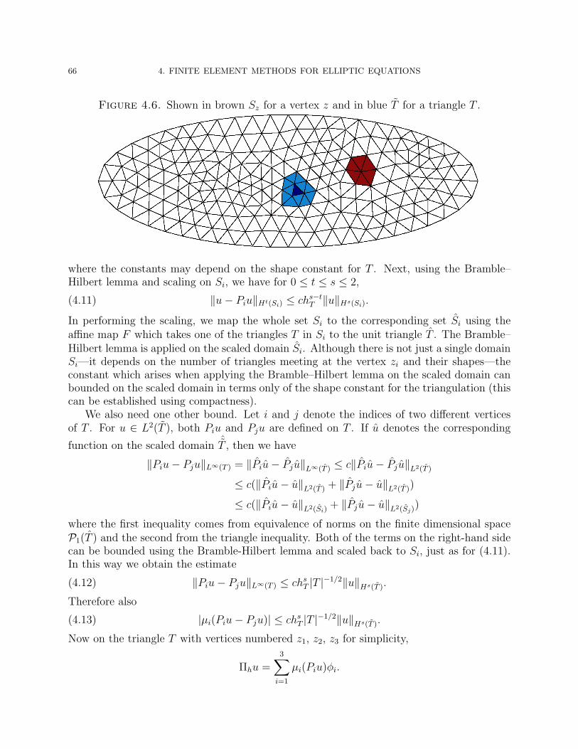
66 4. FINITE ELEMENT METHODS FOR ELLIPTIC EQUATIONS
Figure 4.6. Shown in brown Sz for a vertex z and in blue T for a triangle T .
where the constants may depend on the shape constant for T . Next, using the Bramble–Hilbert lemma and scaling on Si, we have for 0 ≤ t ≤ s ≤ 2,
(4.11) ‖u− Piu‖Ht(Si) ≤ chs−tT ‖u‖Hs(Si).
In performing the scaling, we map the whole set Si to the corresponding set Si using theaffine map F which takes one of the triangles T in Si to the unit triangle T . The Bramble–Hilbert lemma is applied on the scaled domain Si. Although there is not just a single domainSi—it depends on the number of triangles meeting at the vertex zi and their shapes—theconstant which arises when applying the Bramble–Hilbert lemma on the scaled domain canbounded on the scaled domain in terms only of the shape constant for the triangulation (thiscan be established using compactness).
We also need one other bound. Let i and j denote the indices of two different verticesof T . For u ∈ L2(T ), both Piu and Pju are defined on T . If u denotes the corresponding
function on the scaled domain ˆT , then we have
‖Piu− Pju‖L∞(T ) = ‖Piu− Pju‖L∞(T ) ≤ c‖Piu− Pju‖L2(T )
≤ c(‖Piu− u‖L2(T ) + ‖Pju− u‖L2(T ))
≤ c(‖Piu− u‖L2(Si)+ ‖Pju− u‖L2(Sj))
where the first inequality comes from equivalence of norms on the finite dimensional spaceP1(T ) and the second from the triangle inequality. Both of the terms on the right-hand sidecan be bounded using the Bramble-Hilbert lemma and scaled back to Si, just as for (4.11).In this way we obtain the estimate
(4.12) ‖Piu− Pju‖L∞(T ) ≤ chsT |T |−1/2‖u‖Hs(T ).
Therefore also
(4.13) |µi(Piu− Pju)| ≤ chsT |T |−1/2‖u‖Hs(T ).
Now on the triangle T with vertices numbered z1, z2, z3 for simplicity,
Πhu =3∑i=1
µi(Piu)φi.

8. A POSTERIORI ERROR ESTIMATES AND ADAPTIVITY 67
Since P1u is a linear polynomial on T ,
u− Πhu = (u− P1u)−3∑i=2
µi(Piu− P1u)φi.
The first term on the right hand side is bounded using (4.11):
‖u− P1u‖Ht(T ) ≤ chs−tT ‖u‖Hs(T ).
For the second term we have
‖µi(Piu− P1u)φi‖Ht(T ) ≤ ‖Piu− P1u‖L∞(T )‖φi‖Ht(T ),
which satisfies the desired bound by (4.10) and (4.13).For the next section an important special case of (4.9) is
(4.14) ‖u− Πhu‖L2(T ) ≤ chT‖u‖H1(T ).
Another case is H1 boundedness:
(4.15) ‖u− Πhu‖H1(T ) ≤ c‖u‖H1(T ).
We draw one more conclusion, which we will need below. Let T denote the unit triangle,and e one edge of it. The trace theorem then tells us that
‖u‖2L2(e) ≤ c(‖u‖2
L2(T )+ ‖ grad u‖2
L2(T )), u ∈ H1(T ).
If we use linear scaling to an arbitrary triangle, we get
‖u‖2L2(e) ≤ c(h−1
T ‖u‖2L2(T ) + hT‖ gradu‖2
L2(T )), u ∈ H1(T ),
where the constant depends only on the shape constant of T . If we now apply this with ureplaced by u−Πhu and use (4.14) and (4.15), we get this bound for the Clement interpolant:
(4.16) ‖u− Πhu‖L2(e) ≤ ch1/2e ‖u‖H1(T ),
where he is the length of the edge e, T is a triangle containing e, and c depends only on theshape constant for the mesh.
8.2. The residual and the error. Consider our usual model problem
− div a gradu = f in Ω, u = 0 on ∂Ω,
with a continuous positive coefficient a on Ω and f ∈ L2. The weak formulation is to findu ∈ V satisfying
b(u, v) = F (v), v ∈ V,where V = H1(Ω) and
b(w, v) =
∫a gradw · grad v dx, F (v) =
∫fv dx, w, v ∈ V.
The bilinear form is bounded and coercive on H1:
|b(w, v)| ≤M‖w‖1‖v‖1, b(v, v) ≥ γ‖v‖21, w, v ∈ V.
Now let U ∈ V be any function (we will be interested in the case where U = uh, a finiteelement approximation of u). The residual in U is the linear functional R(U) ∈ V ∗ given by
R(U)w = F (w)− b(U,w), w ∈ V.

68 4. FINITE ELEMENT METHODS FOR ELLIPTIC EQUATIONS
Clearly R(U)w = b(u−U,w). It follows immediately that |R(U)w| ≤M‖u−U‖1‖w‖1 for allw ∈ V , or, equivalently, that ‖R(U)‖V ∗ ≤M‖u−U‖1. On the other hand, taking w = u−Uand using the coercivity, we get γ‖u− U‖2
1 ≤ R(U)(u− U) ≤ ‖R(U)‖V ∗‖u− U‖1. Thus
M−1‖R(U)‖V ∗ ≤ ‖u− U‖1 ≤ γ−1‖R(U)‖V ∗ .
In short, the V ∗ norm of the residual R(U) is equivalent to the H1 norm of the error u−U .
8.3. Estimating the residual. Now let Vh be the Lagrange finite element subspaceof V corresponding to some mesh Th and some polynomial degree r, and let uh be thecorresponding finite element solution. We have just seen that we may estimate the error‖u− uh‖1 be estimating the V ∗ error in the residual
R(uh)w = F (w)− b(uh, w), w ∈ V.
This quantity does not involve the unknown solution u, so we may hope to compute it aposteriori, i.e., after we have computed uh.
Next we use integration by parts on each element T of the mesh to rewrite R(uh)w:
R(uh)w =∑T∈Th
∫T
(fw − a graduh · gradw) dx
=∑T
∫T
(f + div a graduh)w dx−∑T
∫∂T
a∂uh∂nT
w ds.
Consider the final sum. We can split each integral over ∂T into the sum of the integrals ofthe three edges of T . Each edge e which is not contained in the boundary comes in twice.For such an edge, let T− and T+ be the two triangles which contain e and set
Re(uh) = −a(∂uh|T−∂nT−
+∂uh|T+
∂nT+
)∈ L2(e)
on e. Since nT− = −nT+ the term in parenthesis is the jump in the normal derivative of uhacross the edge e. Also, for T ∈ Th, we set RT (uh) = f + div a graduh ∈ L2(T ). Then
(4.17) R(uh)w =∑T
∫T
RT (uh)w dx+∑e∈E0
∫e
Re(uh)w ds.
Next we use Galerkin orthogonality : since uh is the finite element solution, we have
b(u− uh, v) = 0, v ∈ Vh.
In terms of the residual this says that
R(uh)w = R(uh)(w − v), v ∈ Vh.
In particular, we may choose v = Πhw, the Clement interpolant in this equation. Combiningwith (4.17) (with w replaced by w − Πhw) we get(4.18)
R(uh)w = R(uh)(w − Πhw) =∑T
∫T
RT (uh)(w − Πhw) dx+∑e∈E0
∫e
Re(uh)(w − Πhw) ds.

8. A POSTERIORI ERROR ESTIMATES AND ADAPTIVITY 69
Now we bound the terms on the right hand side of (4.18) for w ∈ H1. First we use (4.14)to get∫
T
RT (uh)(w − Πhw) dx ≤ ‖RT (uh)‖L2(T )‖w − Πhw‖L2(T ) ≤ chT‖RT (uh)‖L2(T )‖w‖H1(T ).
Therefore
|∑T
∫T
RT (uh)(w − Πhw) dx| ≤
(∑T
h2T‖RT (uh)‖2
L2(T )
)1/2(∑T
‖w‖2H1(T )
)1/2
.
Using shape regularity,∑
T ‖w‖2L2(T )
≤ c‖w‖2H1(Ω), and so we have
(4.19) |∑T
∫T
RT (uh)(w − Πhw) dx| ≤ c
(∑T
h2T‖RT (uh)‖2
L2(T )
)1/2
‖w‖1.
In a similar way, but using (4.16), we get
(4.20) |∑e∈E0
∫e
Re(uh)(w − Πhw) ds| ≤ c
(∑e
he‖Re(uh)‖2L2(e)
)1/2
‖w‖1.
Combining (4.18), (4.19), and (4.20), we get
|R(uh)w| ≤ c
(∑T
h2T‖RT (uh)‖2
L2(T ) +∑e
he‖Re(uh)‖2L2(e)
)1/2
‖w‖1,
or
‖R(uh)‖V ∗ ≤ c
(∑T
h2T‖RT (uh)‖2
L2(T ) +∑e
he‖Re(uh)‖2L2(e)
)1/2
.
In view of the equivalence of the V ∗ norm of the residual and the H1 norm of the error, thisgives us the a posteriori error estimate
(4.21) ‖u− uh‖1 ≤ c
(∑T
h2T‖RT (uh)‖2
L2(T ) +∑e
he‖Re(uh)‖2L2(e)
)1/2
,
which is a key result.
8.4. A posteriori error indicators. The a posteriori error estimate (4.21) containsterms associated to each triangle and to each interior edge. We are going to base ouradaptive strategy on refining those triangles for which the corresponding quantity for eitherthe triangle itself or for one of its edges is large. Therefore we associate to each triangle anerror indicator consisting of the sum of these terms:
η2T := h2
T‖RT (uh)‖2L2(T ) +
1
2
∑e⊂∂T
he‖Re(uh)‖2L2(e)

70 4. FINITE ELEMENT METHODS FOR ELLIPTIC EQUATIONS
The factor of 1/2 is usually used, to account for the fact that each edge belongs to twotriangles. In terms of the error indicators, we can rewrite the a posteriori estimate as
‖u− uh‖1 ≤ c
(∑T
η2T
)1/2
.
Our basic adaptive strategy then proceed via the following SOLVE-ESTIMATE-MARK-REFINE loop:
• SOLVE: Given a mesh, compute uh• ESTIMATE: For each triangle T compute ηT . If (
∑T η
2T )1/2 ≤ tol, quit.
• MARK: Mark those elements T for which ηT is too large for refinement.• REFINE: Create a new mesh with the marked elements refined.
We have already seen how to carry out the SOLVE and ESTIMATE steps. There are anumber of possible strategies for choosing which elements to mark. One of the simplest ismaximal marking. We pick a number ρ between 0 and 1, compute ηmax = maxT ηT , and refinethose elements T for ηT ≥ ρηmax. Another approach, which is usually preferred is Dorflermarking, in which a collection of elements S is marked so that
∑T∈S η
2T ≥ ρ2
∑T∈Th
η2T , i.e.,
we mark enough elements that they account for a given portion ρ of the total error. Theprogram on the next page shows one way to implement this.
Once we have marked the elements, there is the question of how to carry out the refine-ment to be sure that all the marked elements are refined and there is not too much additionalrefinement. In 2-dimensions this is quite easy. Most schemes are based either on dividingeach triangle in two, or dividing the marked triangles into 4 congruent triangles. Generally,after refining the marked elements, additional elements have to be refined to avoid hangingnodes in which a vertex of an element fall in the interior of the edge of a neighboring ele-ment. In 3-dimensions things are more complicated, but good refinement schemes (whichretain shape regularity and avoid hanging nodes) are known.
8.5. Examples of adaptive finite element computations. On the next page wepresent a bare-bones adaptive Poisson solver written in FEniCS, displayed on the next page.This code uses Lagrange piecewise linear finite elements to solve the Dirichlet problem
−∆u = 1 in Ω, u = 0 on ∂Ω,
with Ω an L-shaped domain and f ≡ 1, with the error indicators and marking strategydescribed above. The solution behaves like r2/3 sin(2θ/3) in a neighborhood of the reentrantcorner, and so is not in H2. The results can be seen in Figure 4.7. The final mesh has 6,410elements, all right isoceles triangles, with hypotenuse length h ranging from 0.044 to 0.002.If we used a uniform mesh with the smallest element size, this would require over 3 millionelements. Figure 4.8 displays an adaptive mesh in 3D.

8. A POSTERIORI ERROR ESTIMATES AND ADAPTIVITY 71
"""
Adaptive Poisson solver using a residual-based energy-norm error
estimator
eta_h**2 = sum_T eta_T**2
with
eta_T**2 = h_T**2 ||R_T||_T**2 + c h_T ||R_dT||_dT**2
where
R_T = f + div grad u_h
R_dT = 2 avg(grad u_h * n) (2*avg is jump, since n switches sign across edges)
and a Dorfler marking strategy
Adapted by Douglas Arnold from code of Marie Rognes
"""
from dolfin import *
from sys import stdin
from numpy import zeros
# Stop when sum of eta_T**2 < tolerance or max_iterations is reached
tolerance = 0.04
max_iterations = 20
# Create initial mesh
mesh = Mesh("l-shape-mesh.xml")
mesh.order()
figure(0) # reuse plotting window
# Define boundary and boundary value for Dirichlet conditions
u0 = Constant(0.0)
def boundary(x, on_boundary):
return on_boundary
# SOLVE - ESTIMATE - MARK - REFINE loop
for i in range(max_iterations):
# *** SOLVE step
# Define variational problem and boundary condition
# Solve variational problem on current mesh
V = FunctionSpace(mesh, "CG", 1)
u = TrialFunction(V)
v = TestFunction(V)
f = Constant(1.0)
a = inner(grad(u), grad(v))*dx
L = f*v*dx
u_h = Function(V)
solve(a==L, u_h, DirichletBC(V, u0, boundary))
— continued on next page —

72 4. FINITE ELEMENT METHODS FOR ELLIPTIC EQUATIONS
# *** ESTIMATE step
# Define cell and edge residuals
R_T = f + div(grad(u_h))
# get the normal to the cells
n = V.cell().n
R_dT = 2*avg(dot(grad(u_h), n))
# Will use space of constants to localize indicator form
Constants = FunctionSpace(mesh, "DG", 0)
w = TestFunction(Constants)
h = CellSize(mesh)
# Assemble squared error indicators, eta_T^2, and store into a numpy array
eta2 = assemble(h**2*R_T**2*w*dx + 4.*avg(h)*R_dT**2*avg(w)*dS) # dS is integral over interior edges only
eta2 = eta2.array()
# compute maximum and sum (which is the estimate for squared H1 norm of error)
eta2_max = max(eta2)
sum_eta2 = sum(eta2)
# stop error estimate is less than tolerance
if sum_eta2 < tolerance:
print "Mesh %g: %d triangles, %d vertices, hmax = %g, hmin = %g, errest = %g" \
% (i, mesh.num_cells(), mesh.num_vertices(), mesh.hmax(), mesh.hmin(), sqrt(sum_eta2))
print "\nTolerance achieved. Exiting."
break
# *** MARK step
# Mark cells for refinement for which eta > frac eta_max for frac = .95, .90, ...;
# choose frac so that marked elements account for a given part of total error
frac = .95
delfrac = .05
part = .5
marked = zeros(eta2.size, dtype=’bool’) # marked starts as False for all elements
sum_marked_eta2 = 0. # sum over marked elements of squared error indicators
while sum_marked_eta2 < part*sum_eta2:
new_marked = (~marked) & (eta2 > frac*eta2_max)
sum_marked_eta2 += sum(eta2[new_marked])
marked += new_marked
frac -= delfrac
# convert marked array to a MeshFunction
cells_marked = MeshFunction("bool", mesh, mesh.topology().dim())
cells_marked.array()[:] = marked
# *** REFINE step
mesh = refine(mesh, cells_marked)
plot(mesh, title="Mesh q" + str(i))
print "Mesh %g: %d triangles, %d vertices, hmax = %g, hmin = %g, errest = %g" \
% (i, mesh.num_cells(), mesh.num_vertices(), mesh.hmax(), mesh.hmin(), sqrt(sum_eta2))
stdin.readline()
plot(mesh)
interactive()

8. A POSTERIORI ERROR ESTIMATES AND ADAPTIVITY 73
Figure 4.7. Adaptive solution of Poisson’s equation by the FEniCS programon the preceding page. Shown are the input mesh, the computed adaptivemesh, and a blow-up of that mesh near the re-entrant corner, as well as thefinal solution.
Figure 4.8. An adaptive mesh in 3-dimensions produced by Michael Holstusing his MC code. (The colors relate to partitioning among processors forparallel computation.)

CHAPTER 5
Time-dependent problems
So far we have considered the numerical solution of elliptic PDEs. In this chapter we willconsider some parabolic and hyperbolic PDEs.
1. Finite difference methods for the heat equation
In this section we consider the Dirichlet problem for the heat equation: find u : Ω ×[0, T ]→ R such that
∂u
∂t(x, t)−∆u(x, t) = f(x, t), x ∈ Ω, 0 ≤ t ≤ T,(5.1)
u(x, t) = 0, x ∈ ∂Ω, 0 ≤ t ≤ T.(5.2)
Since this is a time-dependent problem, we also need an initial condition:
u(x, 0) = u0(x), x ∈ Ω.
For simplicity, we will assume Ω = (0, 1)× (0, 1) is the unit square in R2 (or the unit intervalin R). Let us consider first discretization in space only, which we have already studied.Following the notations we used in Chapter 2, we use a mesh with spacing h = 1/N , and letΩh be the set of interior mesh points, Γh the set of boundary mesh points, and Ωh = Ωh∪Γh.The semidiscrete finite difference method is: find uh : Ωh × [0, T ]→ R such at
∂uh∂t
(x, t)−∆huh(x, t) = f(x, t), x ∈ Ωh, 0 ≤ t ≤ T,
uh(x, t) = 0, x ∈ ∂Ωh, 0 ≤ t ≤ T.
uh(x, 0) = u0(x), x ∈ Ωh.
If we let Umn(t) = uh((mh, nh), t), then we may write the first equation as
U ′mn(t)− Um+1,n(t) + Um−1,n(t) + Um,n+1(t) + Um,n−1(t)− 4Umn(t)
h2= fmn(t),
0 < m,n < N, 0 ≤ t ≤ T.
Thus we have a system of (n−1)2 ordinary differential equations, with given initial conditions.One could feed this system of ODEs to an ODE solver. But we shall consider simple ODE
solution schemes, which are, after all, themselves finite difference schemes, and analyze themdirectly. We shall focus on three simple schemes, although there are much more sophisticatedpossibilities.
For a system of ODEs, find u : [0, T ]→ Rm such that
u′(t) = f(t, u(t)), 0 ≤ t ≤ T, u(0) = u0,
75

76 5. TIME-DEPENDENT PROBLEMS
(where f : [0, T ]×Rm → Rm, u0 ∈ Rm) the simplest discretization is Euler’s method. For agiven timestep k > 0, let tj = jk, j = 0, 1, . . ., and define uj = uh(tj) ∈ Rm for j = 0, 1, . . .by uh(0) = u(0), and
uj+1 − ujk
= f(tj, uj), j = 0, 1, . . . .
Explicitly,uj+1 = uj + kf(tj, uj), j = 0, 1, . . . .
An alternative method is the backward Euler method or implicit Euler method
uj+1 − ujk
= f(tj+1, uj+1), j = 0, 1, . . . .
This method involves solving the algebraic system
uj+1 − kf(tj+1, uj+1) = uj, j = 0, 1, . . . .
This is a linear or nonlinear algebraic system according to whether f is linear or nonlinearin u, i.e., according to whether the original ODE system is linear or nonlinear.
1.1. Forward differences in time. Now consider the application of Euler’s methodto the semidiscretized heat equation. We take the timestep k = T/M for some integer M ,so that the discrete time values are 0, k, 2k, . . . , T = Mk. Writing U j
mn for uh((mh, nh), jk)we get the explicit method
(5.3)U j+1mn − U j
mn
k− (∆hU)jmn = f jmn,
i.e.,U j+1mn = U j
mn + k[(∆hU)jmn + f jmn], 0 < m,n < N, j = 0, 1 . . . .
This is called the forward-centered difference method for the heat equation, because it usesforward differences in time and centered differences in space.
We shall analyze the forward-centered scheme (5.3) as usual, by establishing consistencyand stability. Let ujmn = u((mh, nh), tj) denote the restriction of the exact solution, theconsistency error is just
Ejmn : =
uj+1mn − ujmn
k− (∆hu)jmn − f jmn(5.4)
=
[uj+1mn − ujmn
k− (∆hu)jmn
]−[(
∂u
∂t−∆u
)((mh, nh), jk)
].(5.5)
In Chapter 2 we used Taylor’s expansion to get∣∣(∆hu)jmn −∆u((mh, nh), jk)∣∣ ≤ c1h
2,
wherec1 = (‖∂4u/∂x4‖L∞(Ω×[0,T ]) + ‖∂4u/∂y4‖L∞(Ω×[0,T ]))/12.
Even easier is ∣∣∣∣uj+1mn − ujmn
k− ∂u
∂t((mh, nh), jk)
∣∣∣∣ ≤ c2k,
where c2 = ‖∂2u/∂t2u‖L∞/2. Thus
|Ejmn| ≤ c(k + h2),
1. FINITE DIFFERENCE METHODS FOR THE HEAT EQUATION 77
with c = max(c1, c2).Next we establish a stability result. Suppose that a mesh function U j
mn satisfies (5.3).We want to bound an appropriate norm of the mesh function in terms of an appropriatenorm of the function f jmn on the right hand side. For the norm, we use the max norm:
‖U‖L∞ = max0≤j≤M
max0≤m,n≤N
|U jmn|.
Write Kj = max0≤m,n≤N |U jmn|, and F j = max0≤m,n≤N |f jmn|. From (5.3), we have
U j+1mn = (1− 4k
h2)U j
mn +k
h2(U j
m−1,n + U jm+1,n + U j
m,n−1 + U jm,n+1) + kf jmn.
Now we make the assumption that 4k/h2 ≤ 1. Then the 5 coefficients of U on the righthand side are all nonnegative numbers which add to 1, so it easily follows that
Kj+1 ≤ Kj + kF j.
Therefore K1 ≤ K0 + kF 0, K2 ≤ K0 + k(F 0 + F 1), etc. Thus max0≤j≤M Kj ≤ K0 +T max0≤j<M F j, where we have used that kM = T . Thus, if U satisfies (5.3), then
(5.6) ‖U‖L∞ ≤ ‖U0‖L∞(Ωh) + T‖f‖L∞ ,
which is a stability result. We have thus shown stability under the condition that k ≤ h2/4.We say that the forward-centered difference method for the heat equation is conditionallystable.
Now we apply this stability result to the error ejmn = ujmn − U jmn, which satisfies
ej+1mn − ejmn
k− (∆he)
jmn = Ej
mn,
with E the consistency error (so ‖E‖L∞ ≤ c(k + h2)). Note that E0mn = 0, so the stability
result gives
‖e‖L∞ ≤ T‖E‖L∞ .
Using our estimate for the consistency error, we have proven the following theorem.
Theorem 5.1. Let u solve the heat equation (5.1), and let U jmn be determined by the
forward-centered finite difference method with mesh size h = 1/N and timestep k = T/M .Suppose that k ≤ h2/4. Then
max0≤j≤M
max0≤m,n≤N
|u((mh, nh), jk)− U jmn| ≤ C(k + h2),
where C = cT with c as above.
In short, ‖u− uh‖L∞ = O(k + h2).The requirement that 4k/h2 ≤ 1 is not needed for consistency. But it is required to prove
stability, and a simple example shows that it is necessary for convergence. See Figure 5.1.An even simpler example would be the 1D case, for which we obtain stability under thecondition k ≤ h2/2.

78 5. TIME-DEPENDENT PROBLEMS
Figure 5.1. Centered differences in space and forward differences in timefor the Dirichlet problem for the heat equation on the unit square. The meshsize is h = 1/20, and the timestep is k = 1/800 on the left and k = 1/1600 onthe right. On the left we show the result after 18 time steps, i.e., t = 18/800 =.0225. On the right we show the result after 36 time steps (the same time).The computation on the right remains stable for long times.
1.2. Backward differences in time. Next we consider of backward differences in time,i.e., the backward Euler method to solve the semidiscrete system. Then (5.3) becomes
(5.7)U j+1mn − U j
mn
k− (∆hU)j+1
mn = f j+1mn .
This is now an implicit method. Instead of writing down uj+1h explicitly in terms of ujh, we
need to solve for the vector of its values, U j+1mn , from a system of linear equations:
U j+1mn − k∆hU
j+1mn = U j
mn + kf j+1mn , 0 < m,n < N,
or, written out,
(5.8) (1 + 4µ)U j+1mn − µ(U j+1
m+1,n + U j+1m−1,n + U j+1
m,n+1 + U j+1m,n−1) = U j
mn + kf j+1mn ,
with µ = k/h2. This is a sparse system of (N − 1)2 equations in (N − 1)2 unknowns withthe same sparsity pattern as ∆h. Since −∆h is symmetric and positive definite, this system,whose matrix is I − k∆h, is as well.
Remark. The computational difference between explicit and implicit methods was verysignificant before the advent of fast solvers, like multigrid. Since such solvers reduce thecomputational work to the order of the number of unknowns, they are not so much slowerthan explicit methods.
Now suppose that (5.8) holds. Let Kj again denote the maximum of |U jmn|. Then there
exists m,n such that Kj+1 = sU j+1mn where s = ±1. Therefore sU j+1
mn ≥ sU j+1m+1,n and similarly
for each of the other three neighbors. For this particular m, n, we multiply (5.8) by s andobtain
Kj+1 = sU j+1mn ≤ sU j
mn + skf j+1mn ≤ Kj + k‖f j+1‖L∞ .
From this we get the stability result (5.6) as before, but now the stability is unconditional:it holds for any h, k > 0. We immediately obtain the analogue of the convergence theoremTheorem 5.1 for the backward-centered method.

1. FINITE DIFFERENCE METHODS FOR THE HEAT EQUATION 79
Theorem 5.2. Let u solve the heat equation (5.1), and let U jmn be determined by the
backward-centered finite difference method with mesh size h = 1/N and timestep k = T/M .Then
max0≤j≤M
max0≤m,n≤N
|u((mh, nh), jk)− U jmn| ≤ C(k + h2),
where C = cT with c as above.
1.3. Fourier analysis. As we did for the Poisson problem, we can use Fourier analysisto analyze difference schemes for the heat equation. Recall that for a mesh function v on Ωh
we defined the norm
‖u‖2h = h2
N−1∑m=1
N−1∑n=1
|u(mh, nh)|2,
and the corresponding inner product. We then showed that −∆h had an orthogonal basisof eigenfunctions φmn with corresponding eigenvalues satisfying
2π2 ≈ λ1,1 ≤ λmn ≤ λN−1,N−1 < 8/h2.
Consider now the forward-centered difference equations for the heat equation ∂u/∂t = ∆u,with homogeneous Dirichlet boundary data, and given initial data u0 (for simplicity weassume f ≡ 0). We have
U j+1mn = GU j
mn,
where the G = I + k∆h. By iteration, we have
‖U j‖ ≤ ‖G‖j‖U0‖.
Thus we have L2 stability if and only if the spectral radius of G is bounded by 1. Now theeigenvalues 1− kλmn, so they satisfy 1− 8k/h2 < µ < 1, so the spectral radius condition issatisfies if 1− 8k/h2 ≥ −1, i.e., k ≤ h2/4. In this way, Fourier analysis leads us to the sameconditional stability condition we obtained above.
If we consider instead the backward-centered difference scheme, then the correspondingoperator G is G = (I + k∆h)
−1 with eigenvalues (1 + kλmn)−1, which has spectral radiusbounded by 1 for any k > 0. Thus we obtain unconditional stability.
1.4. Crank–Nicolson. Although we are free to choose the timestep and space typeas we like for the backward-centered method, accuracy considerations still indicate that weshould take k = O(h2), so very small timesteps. It is natural to seek a method which is secondorder in time as well as space. If we use the trapezoidal method for time discretization, theresulting fully discrete scheme is called the Crank–Nicolson method. It is an implicit methodgiven by
U j+1mn − U j
mn
k− 1
2[(∆hU)j+1
mn + (∆hU)jmn] =1
2[f jmn + f j+1
mn ].
We leave it as an exercise to show that the Crank–Nicolson scheme is unconditionally stablescheme with respect to the L2 norm, with error O(h2 + k2).

80 5. TIME-DEPENDENT PROBLEMS
2. Finite element methods for the heat equation
In this section we consider the initial boundary value problem for the heat equation
∂u
∂t(x, t)− div a(x) gradu(x, t) = f(x, t), x ∈ Ω, 0 ≤ t ≤ T,
u(x, t) = 0, x ∈ ∂Ω, 0 ≤ t ≤ T,
u(x, 0) = u0(x), x ∈ Ω.
We have allowed the thermal conductivity a to be variable, assuming only that it is boundedabove and below by positive constants, since this will cause no additional complications. Wecould easily generalize further, allowing a variable specific heat (coefficient of ∂u/∂t), lowerorder terms, and different boundary conditions.
Now we consider finite elements for spatial discretization. To derive a weak formulation,we multiply the heat equation (5.1) by a test function v(x) ∈ H1(Ω) and integrate over Ω.This gives∫
Ω
∂u
∂t(x, t)v(x) dx+
∫Ω
a(x) gradu(x, t) · grad v(x) dx =
∫Ω
f(x, t)v(x) dx, 0 ≤ t ≤ T.
Writing 〈 · , · 〉 for the L2(Ω) inner product and b(w, v) =∫
Ωa gradw · grad v dx, we may
write the weak formulation as
〈∂u∂t, v〉+ b(u, v) = 〈f, v〉, v ∈ H1(Ω), 0 ≤ t ≤ T.
For the finite element method it is often useful to think of u(x, t) as a function of t taking
values in functions of x. Specifically, we may think of u mapping t ∈ [0, T ] to u(·, t) ∈ H1(Ω).
Specifically, we may seek the solution u ∈ C1([0, T ], H1(Ω)), which means that u(·, t) ∈H1(Ω) for each t, that u is differentiable with respect to t, and that ∂u(·, t)/∂t ∈ H1(Ω) for
all t. Thus when we write u(t), we mean the function u(·, t) ∈ H1(Ω).
Now let Vh ⊂ H1(Ω) denote the usual space of Lagrange finite elements of degree r withrespect to a triangulation of Ω. For a semidiscrete finite element approximation we seek uhmapping [0, T ] into Vh, i.e., uh ∈ C1([0, T ], Vh), satisfying
(5.9) 〈∂uh∂t
, v〉+ b(uh, v) = 〈f, v〉, v ∈ Vh, 0 ≤ t ≤ T.
We also need to specify an initial condition for uh. For this we choose some u0h ∈ Vh which
approximates u0 (common choices are the L2 projection or the interpolant).We now show that this problem may be viewed as a system of ODEs. For this let φi,
1 ≤ i ≤ D be a basis for Vh (for efficiency we will choose a local basis). We may then write
uh(x, t) =D∑j=1
αj(t)φj(x).
Plugging this into (5.9) and taking the test function v = φi, we get∑j
〈φj, φi〉α′j(t) +∑j
b(φj, φi)αj(t) = 〈f, φi〉.

2. FINITE ELEMENT METHODS FOR THE HEAT EQUATION 81
In terms of the mass matrix, stiffness matrix, and load vector:
Mij = 〈φj, φi〉, Aij = 〈φj, φi〉, Fi(t) = 〈f, φi〉,this can be written
Mα′(t) + Aα(t) = F (t), 0 ≤ t ≤ T.
This is a system of linear ODEs for the unknown coefficients α = (αj(t)). The initialcondition uh(0) = u0
h can be written α(0) = α0 where u0h =
∑j α
0jφj.
We now turn to fully discrete approximation using the finite element method for dis-cretization in space, and finite differences for discretization in time. Consider first usingEuler’s method for time discretization. This leads to the system
Mαj+1 − αj
k+ Aαj = F j,
or
Mαj+1 = Mαj + k(−Aαj + F j).
Notice that for finite elements this method is not truly explicit, since we have to solve anequation involving the mass matrix at each time step.
The backward Euler’s method
Mαj+1 − αj
k+ Aαj+1 = F j+1,
leads to a different linear system at each time step:
(M + kA)αj+1 = Mαj + kF j+1,
while Crank–Nicolson would give
(M +k
2A)αj+1 = (M − k
2A)αj +
k
2(F j + F j+1).
2.1. Analysis of the semidiscrete finite element method. Before analyzing a fullydiscrete finite element scheme, we analyze the convergence of the semidiscrete scheme, sinceit is less involved. The key to the analysis of the semidiscrete finite element method is tocompare uh not directly to u, but rather to an appropriate representative wh ∈ C1([0, T ], Vh).For wh we choose the elliptic projection of u, defined by
(5.10) b(wh, v) = b(u, v), v ∈ Vh, 0 ≤ t ≤ T.
From our study of the finite element method for elliptic problems, we have the L2 estimate
(5.11) ‖u(t)− wh(t)‖ ≤ chr+1‖u(t)‖r+1, 0 ≤ t ≤ T.
If we differentiate (5.10), we see that ∂wh/∂t is the elliptic projection of ∂u/∂t, so
‖∂u∂t
(t)− ∂wh∂t
(t)‖ ≤ chr+1‖∂u∂t
(t)‖r+1, 0 ≤ t ≤ T.
Now
(5.12)〈∂wh∂t
, v〉+ b(wh, v) = 〈∂wh∂t
, v〉+ b(u, v)
= 〈∂(wh − u)
∂t, v〉+ 〈f, v〉, v ∈ Vh, 0 ≤ t ≤ T.

82 5. TIME-DEPENDENT PROBLEMS
Let yh = wh − uh. Subtracting (5.9) from (5.12), we get
〈∂yh∂t
, v〉+ b(yh, v) = 〈∂(wh − u)
∂t, v〉, v ∈ Vh, 0 ≤ t ≤ T.
Now, for each t we choose v = yh(t) ∈ Vh. Note that for any function y ∈ C1([0, T ];L2(Ω)),
‖y‖ ddt‖y‖ =
1
2
d
dt‖y‖2 = 〈∂y
∂t, y〉.
Thus we get
(5.13) ‖yh‖d
dt‖yh‖+ b(yh, yh) = 〈∂(wh − u)
∂t, yh〉 ≤ ‖
∂(wh − u)
∂t‖‖yh‖,
sod
dt‖yh‖ ≤ ‖
∂(wh − u)
∂t‖ ≤ chr+1‖∂u
∂t(t)‖r+1.
This holds for each t. Integrating over [0, t], we get
‖yh(t)‖ ≤ ‖yh(0)‖+ chr+1‖∂u∂t‖L1([0,T ];Hr+1(Ω)).
For yh(0) we have
‖yh(0)‖ = ‖wh(0)− uh(0)‖ ≤ ‖wh(0)− u(0)‖+ ‖u0− uh(0)‖ ≤ chr+1‖u0‖r+1 + ‖u0− uh(0)‖.
Thus, assuming that the exact solution is sufficiently smooth and the initial data uh(0) ischosen so that ‖u0 − uh(0)‖ = O(hr+1), we have
‖yh‖L∞([0,T ];L2(Ω)) = O(hr+1).
Combining this estimate with the elliptic estimate (5.11) we get an estimate on the error
‖u− uh‖L∞([0,T ];L2(Ω)) = O(hr+1).
Remark. We can put this analysis into the framework of consistency and stability in-troduced in Section 3. We take our discrete solution space Xh as C1([0, T ];Vh), and thediscrete operator Lh : Xh → Yh := C([0, T ];V ∗h ) is
(Lhuh)(v) = 〈∂uh∂t
, v〉+ b(uh, v), uh ∈ Xh, v ∈ Vh, 0 ≤ t ≤ T.
Thus our numerical method is to find uh ∈ Xh such that Lhuh = Fh, where
Fh(v) =
∫fv dx, v ∈ Vh, 0 ≤ t ≤ T.
As a representative rhu ∈ Xh of the exact solution u we use the elliptic projection wh. Thenthe consistency error is given by
E(v) := 〈∂wh∂t
, v〉+ b(wh, v)− 〈f, v〉, v ∈ Vh, 0 ≤ t ≤ T.
In the first part of our analysis we showed that
E(v) = 〈∂(wh − u)
∂t, v〉,

2. FINITE ELEMENT METHODS FOR THE HEAT EQUATION 83
so |||E||| = O(hr+1), where the norm we use on Yh is
|||E||| =∫ T
0
sup06=v∈Vh
|E(v)|‖v‖
dt.
The second part of the analysis was a stability result. Essentially we showed that if uh ∈ Xh
and Fh ∈ Yh satisfy Lhuh = Fh, then
max0≤t≤T
‖uh‖ ≤ ‖uh(0)‖+ |||Fh|||.
Remark. In the case of finite elements for elliptic problems, we first got an estimatein H1, then an estimate in L2, and I mentioned that there are others possible. In thecase of the parabolic problem, there are many other estimates we could derive in differentnorms in space or time or both. For example, by integrating (5.13) in time we get that‖yh‖L2([0,T ];H1(Ω)) = O(hr+1). For the elliptic projection we have ‖u − wh‖H1(Ω) = O(hr) foreach t, so the triangle inequality gives ‖u− uh‖L2([0,T ];H1(Ω)) = O(hr).
2.2. Analysis of a fully discrete finite element method. Now we turn to theanalysis of a fully discrete scheme: finite elements in space and backward Euler in time.Writing ujh for uh(·, jk) (with k the time step), the scheme is
(5.14) 〈uj+1h − ujhk
, v〉+ b(uj+1, v) = 〈f j+1, v〉, v ∈ Vh, j = 0, 1, . . . .
We initialize the iteration by choosing u0h ∈ Vh to be, e.g., the interpolant, L2 projection, or
elliptic projection. Notice that, at each time step, we have to solve the linear system
(M + kA)αj+1 = Mαj + kF j+1,
where αj is the vector of coefficients of ujh with respect to a basis, and M , A, and F , are themass matrix, stiffness matrix, and load vector respectively.
To analyze this scheme, we proceed as we did for the semidiscrete scheme, with someextra complications coming from the time discretization. In particular, we continue to usethe elliptic projection wh as a representative of u. Thus the consistency error is given by
〈wj+1h − wjhk
,v〉+ b(wj+1h , v)− 〈f j+1, v〉
= 〈uj+1 − uj
k, v〉+ b(uj+1, v)− 〈f j+1, v〉+ 〈(w
j+1h − uj+1)− (wjh − uj)
k, v〉
= 〈uj+1 − uj
k− ∂uj+1
∂t, v〉+ 〈(w
j+1h − uj+1)− (wjh − uj)
k, v〉 = 〈zj, v〉,
where the last line gives the definition of zj. Next we estimate the two terms that comprisezj, in L2. First we have
‖uj+1 − uj
k− ∂uj+1
∂t‖ ≤ k
2‖∂
2u
∂t2‖L∞(L2),
by Taylors theorem. Next,
(wj+1h − uj+1)− (wjh − uj)
k=
1
k
∫ (j+1)k
jk
∂
∂t[wh(s)− u(s)] ds,

84 5. TIME-DEPENDENT PROBLEMS
so
‖(wj+1h − uj+1)− (wjh − uj)
k‖ ≤ chr+1‖∂u
∂t‖L∞([jk,(j+1)k];Hr+1(Ω).
Thus we have obtained a bound on the consistency error:
〈wj+1h − wjhk
, v〉+ b(wj+1h , v)− 〈f j+1, v〉 = 〈zj, v〉, v ∈ Vh, j = 0, 1, . . . .
with
‖zj‖ ≤ c(k‖∂2u
∂t2‖L∞([0,T ];L2(Ω)) + hr+1‖∂u
∂t‖L∞([0,T ];Hr+1(Ω)) =: E, j = 0, 1, . . . .
Combining with the scheme (5.14), we get (for yh = wh − uh)
〈yj+1h − yjhk
, v〉+ b(yj+1h , v) = 〈zj, v〉, v ∈ Vh.
We conclude the argument with a stability argument. Choose v = yj+1h ∈ Vh. This becomes:
‖yj+1h ‖
2 + kb(yj+1h , yj+1
h ) = 〈yjh + kzj, yj+1h 〉,
so‖yj+1
h ‖ ≤ ‖yjh‖+ kE,
and, by iteration,max
0≤j≤M‖yjh‖ ≤ ‖y
0h‖+ TE.
In this way we prove that
max0≤j≤M
‖uj − ujh‖ = O(k + hr+1).
Exercise for the reader: analyze the convergence of the fully discrete finite element methodusing Crank–Nicolson for time discretization. In the stability argument, you will want touse the test function v = (yj+1
h + yjh)/2.