numerical methods for partial di erential equations
TRANSCRIPT

Numerical Methods forPartial Differential Equations
Joachim Schoberl
October 2, 2018

2

Contents
1 Introduction 71.1 Classification of PDEs . . . . . . . . . . . . . . . . . . . . . . . . . . . . . 71.2 Weak formulation of the Poisson Equation . . . . . . . . . . . . . . . . . . 81.3 The Finite Element Method . . . . . . . . . . . . . . . . . . . . . . . . . . 10
2 The abstract theory 132.1 Basic properties . . . . . . . . . . . . . . . . . . . . . . . . . . . . . . . . . 132.2 Projection onto subspaces . . . . . . . . . . . . . . . . . . . . . . . . . . . 162.3 Riesz Representation Theorem . . . . . . . . . . . . . . . . . . . . . . . . . 172.4 Symmetric variational problems . . . . . . . . . . . . . . . . . . . . . . . . 182.5 Coercive variational problems . . . . . . . . . . . . . . . . . . . . . . . . . 19
2.5.1 Approximation of coercive variational problems . . . . . . . . . . . 222.6 Inf-sup stable variational problems . . . . . . . . . . . . . . . . . . . . . . 23
2.6.1 Approximation of inf-sup stable variational problems . . . . . . . . 25
3 Sobolev Spaces 273.1 Generalized derivatives . . . . . . . . . . . . . . . . . . . . . . . . . . . . . 273.2 Sobolev spaces . . . . . . . . . . . . . . . . . . . . . . . . . . . . . . . . . 293.3 Trace theorems and their applications . . . . . . . . . . . . . . . . . . . . . 30
3.3.1 The trace space H1/2 . . . . . . . . . . . . . . . . . . . . . . . . . 363.4 Equivalent norms on H1 and on sub-spaces . . . . . . . . . . . . . . . . . . 393.5 Interpolation Spaces . . . . . . . . . . . . . . . . . . . . . . . . . . . . . . 43
3.5.1 Hilbert space interpolation . . . . . . . . . . . . . . . . . . . . . . . 433.5.2 Banach space interpolation . . . . . . . . . . . . . . . . . . . . . . . 433.5.3 Operator interpolation . . . . . . . . . . . . . . . . . . . . . . . . . 453.5.4 Interpolation of Sobolev Spaces . . . . . . . . . . . . . . . . . . . . 46
3.6 The weak formulation of the Poisson equation . . . . . . . . . . . . . . . . 473.6.1 Shift theorems . . . . . . . . . . . . . . . . . . . . . . . . . . . . . . 48
4 Finite Element Method 514.1 Finite element system assembling . . . . . . . . . . . . . . . . . . . . . . . 534.2 Finite element error analysis . . . . . . . . . . . . . . . . . . . . . . . . . . 554.3 A posteriori error estimates . . . . . . . . . . . . . . . . . . . . . . . . . . 61
3

4 CONTENTS
4.4 Equilibrated Residual Error Estimates . . . . . . . . . . . . . . . . . . . . 69
4.4.1 General framework . . . . . . . . . . . . . . . . . . . . . . . . . . . 69
4.4.2 Computation of the lifting ‖σ∆‖ . . . . . . . . . . . . . . . . . . . . 71
4.5 Non-conforming Finite Element Methods . . . . . . . . . . . . . . . . . . . 73
4.6 hp - Finite Elements . . . . . . . . . . . . . . . . . . . . . . . . . . . . . . 79
4.6.1 Legendre Polynomials . . . . . . . . . . . . . . . . . . . . . . . . . 79
4.6.2 Error estimate of the L2 projection . . . . . . . . . . . . . . . . . . 81
4.6.3 Orthogonal polynomials on triangles . . . . . . . . . . . . . . . . . 83
4.6.4 Projection based interpolation . . . . . . . . . . . . . . . . . . . . . 84
5 Linear Equation Solvers 87
5.1 Direct linear equation solvers . . . . . . . . . . . . . . . . . . . . . . . . . 88
5.2 Iterative equation solvers . . . . . . . . . . . . . . . . . . . . . . . . . . . . 91
5.3 Preconditioning . . . . . . . . . . . . . . . . . . . . . . . . . . . . . . . . . 100
5.4 Analysis of the multi-level preconditioner . . . . . . . . . . . . . . . . . . . 112
6 Mixed Methods 117
6.1 Weak formulation of Dirichlet boundary conditions . . . . . . . . . . . . . 117
6.2 A Mixed method for the flux . . . . . . . . . . . . . . . . . . . . . . . . . . 118
6.3 Abstract theory . . . . . . . . . . . . . . . . . . . . . . . . . . . . . . . . . 119
6.4 Analysis of the model problems . . . . . . . . . . . . . . . . . . . . . . . . 122
6.5 Approximation of mixed systems . . . . . . . . . . . . . . . . . . . . . . . 129
6.6 Supplement on mixed methods for the flux : discrete norms, super-convergence and implementation techniques . . . . . . . . . . . . . . . . . 132
6.6.1 Primal and dual mixed formulations . . . . . . . . . . . . . . . . . 132
6.6.2 Super-convergence of the scalar . . . . . . . . . . . . . . . . . . . . 134
6.6.3 Solution methods for the linear system . . . . . . . . . . . . . . . . 136
6.6.4 Hybridization . . . . . . . . . . . . . . . . . . . . . . . . . . . . . . 136
7 Discontinuous Galerkin Methods 139
7.1 Transport equation . . . . . . . . . . . . . . . . . . . . . . . . . . . . . . . 139
7.1.1 Solvability . . . . . . . . . . . . . . . . . . . . . . . . . . . . . . . . 140
7.2 Discontinuous Galerkin Discretization . . . . . . . . . . . . . . . . . . . . . 141
7.3 Nitsche’s method for Dirichlet boundary conditions . . . . . . . . . . . . . 144
7.3.1 Nitsche’s method for interface conditions . . . . . . . . . . . . . . . 145
7.4 DG for second order equations . . . . . . . . . . . . . . . . . . . . . . . . . 146
7.4.1 Hybrid DG . . . . . . . . . . . . . . . . . . . . . . . . . . . . . . . 147
7.4.2 Bassi-Rebay DG . . . . . . . . . . . . . . . . . . . . . . . . . . . . 148
7.4.3 Matching integration rules . . . . . . . . . . . . . . . . . . . . . . . 148
7.4.4 (Hybrid) DG for Stokes and Navier-Stokes . . . . . . . . . . . . . . 148
CONTENTS 5
8 Applications 1518.1 The Navier Stokes equation . . . . . . . . . . . . . . . . . . . . . . . . . . 151
8.1.1 Proving LBB for the Stokes Equation . . . . . . . . . . . . . . . . . 1538.1.2 Discrete LBB . . . . . . . . . . . . . . . . . . . . . . . . . . . . . . 154
8.2 Elasticity . . . . . . . . . . . . . . . . . . . . . . . . . . . . . . . . . . . . 1578.3 Maxwell equations . . . . . . . . . . . . . . . . . . . . . . . . . . . . . . . 164
9 Parabolic partial differential equations 1719.1 Semi-discretization . . . . . . . . . . . . . . . . . . . . . . . . . . . . . . . 1739.2 Time integration methods . . . . . . . . . . . . . . . . . . . . . . . . . . . 1759.3 Space-time formulation of Parabolic Equations . . . . . . . . . . . . . . . . 177
9.3.1 Solvability of the continuous problem . . . . . . . . . . . . . . . . . 1779.3.2 A first time-discretization method . . . . . . . . . . . . . . . . . . . 1799.3.3 Discontinuous Galerkin method . . . . . . . . . . . . . . . . . . . . 179
10 Second order hyperbolic equations: wave equations 18310.0.1 Examples . . . . . . . . . . . . . . . . . . . . . . . . . . . . . . . . 18310.0.2 Time-stepping methods for wave equations . . . . . . . . . . . . . . 18410.0.3 The Newmark time-stepping method . . . . . . . . . . . . . . . . . 18410.0.4 Methods for the first order system . . . . . . . . . . . . . . . . . . . 186
11 Hyperbolic Conservation Laws 18911.1 A little theory . . . . . . . . . . . . . . . . . . . . . . . . . . . . . . . . . . 190
11.1.1 Weak solutions and the Rankine-Hugoniot relation . . . . . . . . . 19011.1.2 Expansion fans . . . . . . . . . . . . . . . . . . . . . . . . . . . . . 191
11.2 Numerical Methods . . . . . . . . . . . . . . . . . . . . . . . . . . . . . . . 192

6 CONTENTS

Chapter 1
Introduction
Differential equations are equations for an unknown function involving differential opera-tors. An ordinary differential equation (ODE) requires differentiation with respect to onevariable. A partial differential equation (PDE) involves partial differentiation with respectto two or more variables.
1.1 Classification of PDEs
The general form of a linear PDE of second order is: find u : Ω ⊂ Rd → R such that
d∑i,j=1
− ∂
∂xi
(ai,j(x)
∂u(x)
∂xj
)+
d∑i=1
bi(x)∂u(x)
∂xi+ c(x)u(x) = f(x). (1.1)
The coefficients ai,j(x), bi(x), c(x) and the right hand side f(x) are given functions. Inaddition, certain type of boundary conditions are required. The behavior of the PDEdepends on the type of the differential operator
L :=d∑
i,j=1
∂
∂xiai,j
∂
∂xj+
d∑i=1
bi∂
∂xi+ c.
Replace ∂∂xi
by si. Thend∑
i,j=1
siai,jsj +d∑i=1
bisi + c = 0
describes a quartic shape in Rd. We treat the following cases:
1. In the case of a (positive or negative) definite matrix a = (ai,j) this is an ellipse,and the corresponding PDE is called elliptic. A simple example is a = I, b = 0, andc = 0, i..e.
−∑i
∂2u
∂x2i
= f.
7

8 CHAPTER 1. INTRODUCTION
Elliptic PDEs require boundary conditions.
2. If the matrix a is semi-definite, has the one-dimensional kernel spanv, and b ·v 6= 0,then the shape is a parabola. Thus, the PDE is called parabolic. A simple exampleis
−d−1∑i=1
∂2u
∂x2i
+∂u
∂xd= f.
Often, the distinguished direction corresponds to time. This type of equation requiresboundary conditiosn on the d−1-dimensional boundary, and initial conditions in thedifferent direction.
3. If the matrix a has d− 1 positive, and one negative (or vise versa) eigenvalues, thenthe shape is a hyperbola. The PDE is called hyperbolic. The simplest one is
−d−1∑i=1
∂2u
∂x2i
+∂2u
∂x2d
= f.
Again, the distinguished direction often corresponds to time. Now, two initial con-ditions are needed.
4. If the matrix a is zero, then the PDE degenerates to the first order PDE
bi∂u
∂xi+ cu = f.
Boundary conditions are needed at a part of the boundary.
These cases behave very differently. We will establish theories for the individual cases.A more general classicfication, for more positive or negative eigenvalues, and systems ofPDEs is possible. The type of the PDE may also change for different points x.
1.2 Weak formulation of the Poisson Equation
The most elementary and thus most popular PDE is the Poisson equation
−∆u = f in Ω, (1.2)
with the boundary conditions
u = uD on ΓD,∂u∂n
= g on ΓN ,∂u∂n
+ αu = g onΓR.(1.3)
The domain Ω is an open and bounded subset of Rd, where the problem dimension d isusually 1, 2 or 3. For d = 1, the equation is not a PDE, but an ODE. The boundary
1.2. WEAK FORMULATION OF THE POISSON EQUATION 9
Γ := ∂Ω consists of the three non-overlapping parts ΓD, ΓN , and ΓR. The outer unitnormal vector is called n. The Laplace differential operator is ∆ :=
∑di=1
∂2
∂x2i, the normal
derivative at the boundary is ∂∂n
:=∑d
i=1 ni∂∂xi
. Given are the functions f , uD and g inproper function spaces (e.g., f ∈ L2(Ω)). We search for the unknown function u, again, ina proper function space defined later.
The boundary conditions are called
• Dirichlet boundary condition on ΓD. The function value is prescribed,
• Neumann boundary condition on ΓN . The normal derivative is prescribed,
• Robin boundary condition on ΓR. An affine linear relation between the functionvalue and the normal derivative is prescribed.
Exactly one boundary condition must be specified on each part of the boundary.
We transform equation (1.2) together with the boundary conditions (1.3) into its weakform. For this, we multiply (1.2) by smooth functions (called test functions) and integrateover the domain:
−∫
Ω
∆uv dx =
∫Ω
fv dx (1.4)
We do so for sufficiently many test functions v in a proper function space. Next, we applyGauss’ theorem
∫Ω
div p dx =∫
Γp · n ds to the function p := ∇u v to obtain∫
Ω
div(∇u v) dx =
∫Γ
∇u · n v ds
From the product rule there follows div(∇uv) = ∆uv +∇u · ∇v. Together we obtain∫Ω
∇u · ∇v dx−∫
Γ
∂u
∂nv ds =
∫Ω
fv dx.
Up to now, we only used the differential equation in the domain. Next, we incorporatethe boundary conditions. The Neumann and Robin b.c. are very natural (and thus arecalled natural boundary conditions). We simply replace ∂u
∂nby g and −αu + g on ΓN and
ΓR, respectively. Putting unknown terms to the left, and known terms to the right handside, we obtain∫
Ω
∇u · ∇v dx+
∫ΓR
αuv ds−∫
ΓD
∂u
∂nv ds =
∫fv dx+
∫ΓN+ΓR
gv ds.
Finally, we use the information of the Dirichlet boundary condition. We work brute forceand simple keep the Dirichlet condition in strong sense. At the same time, we only allowtest functions v fulfilling v = 0 on ΓD. We obtain the

10 CHAPTER 1. INTRODUCTION
Weak form of the Poisson equation:Find u such that u = uD on ΓD and∫
Ω
∇u · ∇v dx+
∫ΓR
αuv ds =
∫Ω
fv dx+
∫ΓN+ΓR
gv ds (1.5)
∀ v such that v = 0 on ΓD.
We still did not define the function space in which we search for the solution u. A properchoice is
V := v ∈ L2(Ω) : ∇u ∈ [L2(Ω)]d and u|Γ ∈ L2(∂Ω).
It is a complete space, and, together with the inner product
(u, v)V := (u, v)L2(Ω) + (∇u,∇v)L2(Ω) + (u, v)L2(Γ)
it is a Hilbert space. Now, we see that f ∈ L2(Ω) and g ∈ L2(Γ) is useful. The Dirichletb.c. uD must be chosen such that there exists an u ∈ V with u = uD on ΓD. By definitionof the space, all terms are well defined. We will see later, that the problem indeed has aunique solution in V .
1.3 The Finite Element Method
Now, we are developing a numerical method for approximating the weak form (1.5). Forthis, we decompose the domain Ω into triangles T . We call the set T = T triangulation.The set N = xj is the set of nodes. By means of this triangulation, we define the finiteelement space, Vh:
Vh := v ∈ C(Ω) : v|T is affine linear ∀T ∈ T
This is a sub-space of V . The derivatives (in weak sense, see below) are piecewise constant,and thus, belong to [L2(Ω)]2. The function vh ∈ Vh is uniquely defined by its values v(xj)in the nodes xj ∈ N . We decompose the set of nodes as
N = ND ∪Nf ,
where ND are the nodes on the Dirichlet boundary, and Nf are all others (f as free). Thefinite element approximation is defined as
Find uh such that uh(x) = uD(x) ∀x ∈ ND and∫Ω
∇uh · ∇vh dx+
∫ΓR
αuhvh ds =
∫fvh dx+
∫ΓN+ΓR
gvh ds (1.6)
∀ vh ∈ Vh such that vh(x) = 0 ∀x ∈ ND

1.3. THE FINITE ELEMENT METHOD 11
Now it is time to choose a basis for Vh. The most convenient one is the nodal basisϕi characterized as
ϕi(xj) = δi,j. (1.7)
The Kronecker-δ is defined to be 1 for i = j, and 0 else. These are the popular hatfunctions. We represent the finite element solution with respect to this basis:
uh(x) =∑
uiϕi(x) (1.8)
By the nodal-basis property (1.7) there holds uh(xj) =∑
i uiϕi(xj) = uj. We have todetermine the coefficients ui ∈ RN , with N = |N |. The ND := |ND| values according tonodes on ΓD are given explicitely:
uj = uh(xj) = uD(xj) ∀xj ∈ ΓD
The others have to be determined from the variational equation (1.6). It is equivalent tofulfill (1.6) for the whole space vh ∈ Vh : vh(x) = 0 ∀ xj ∈ ND, or just for its basisϕi : xi ∈ Nf associated to the free nodes:
∑i
∫Ω
∇ϕi ·∇ϕj dx+
∫ΓR
αϕiϕj dsui =
∫fϕj dx+
∫ΓN+ΓR
gϕj ds (1.9)
∀ϕj such that xj ∈ NfWe have inserted the basis expansion (1.8). We define the matrix A = (Aji) ∈ RN×N andthe vector f = (fj) ∈ RN as
Aji :=
∫Ω
∇ϕi · ∇ϕj dx+
∫ΓR
αϕiϕj ds,
fj :=
∫fϕj dx+
∫ΓN+ΓR
gϕj ds.
According to Dirichlet- and free nodes they are splitted as
A =
(ADD ADDAfD Aff
)and f =
(fDff
).
Now, we obtain the system of linear equations for u = (ui) ∈ RN , u = (uD, uf ):(I 0
AfD Aff
)(uDuf
)=
(uDff
). (1.10)
At all, we have N coefficients ui. ND are given explicitely from the Dirichlet values. Theseare Nf equations to determine the remaining ones. Using the known uD, we can reformulateit as symmetric system of equations for uf ∈ RNf :
Affuf = ff − AfDuD

12 CHAPTER 1. INTRODUCTION

Chapter 2
The abstract theory
In this chapter we develop the abstract framework for variational problems.
2.1 Basic properties
Definition 1. A vector space V is a set with the operations + : V × V → V and· : R× V → V such that for all u, v ∈ V and λ, µ ∈ R there holds
• u+ v = v + u
• (u+ v) + w = u+ (v + w)
• λ · (u+ v) = λ · u+ λ · v, (λ+ µ) · u = λ · u+ µ · u
Examples are Rn, the continuous functions C0, or the Lebesgue space L2.
Definition 2. A normed vector space (V, ‖ · ‖) is a vector space with the operation ‖.‖ :V → R being a norm, i.e., for u, v ∈ V and λ ∈ R there holds
• ‖u+ v‖ ≤ ‖u‖+ ‖v‖
• ‖λu‖ = |λ| ‖u‖
• ‖u‖ = 0⇔ u = 0
Examples are (C0, ‖ · ‖sup), or (C0, ‖ · ‖L2).
Definition 3. In a complete normed vector space, Cauchy sequences (un) ∈ V N convergeto an u ∈ V . A complete normed vector space is called Banach space.
Examples of Banach spaces are (L2, ‖ · ‖L2), (C0, ‖ · ‖sup), but not (C0, ‖ · ‖L2).
Definition 4. The closure of a normed vector-space (W, ‖ · ‖V ), denoted as W‖·‖V
is thesmallest complete space containing W .
13

14 CHAPTER 2. THE ABSTRACT THEORY
Example: C‖·‖L2 = L2.
Definition 5. A functional or a linear form l(·) on V is a linear mapping l(·) : V → R.The canonical norm for linear forms is the dual norm
‖l‖V ∗ := sup0 6=v∈V
l(v)
‖v‖.
A linear form l is called bounded if the norm is finite. The vector space of all boundedlinear forms on V is called the dual space V ∗.
An example for a bounded linear form is l(·) : L2 → R : v →∫v dx.
Definition 6. A bilinear form A(·, ·) on V is a mapping A : V × V → R which is linearin u and in v. It is called symmetric if A(u, v) = A(v, u) for all u, v ∈ V .
Examples are the bilinear form A(u, v) =∫uv dx on L2, or A(u, v) := uTAv on Rn, where
A is a (symmetric) matrix.
Definition 7. A symmetric bilinear form A(·, ·) is called an inner product if it satisfies
• (v, v) ≥ 0 ∀ v ∈ V
• (v, v) = 0⇔ v = 0
Often, is is denoted as (·, ·)A, (·, ·)V , or simply (·, ·).
An examples on R is uTAv, where A is a symmetric and positive definite matrix.
Definition 8. An inner product space is a vector space V together with an inner product(·, ·)V .
Lemma 9. Cauchy Schwarz inequality. If A(·, ·) is a symmetric bilinear form suchthat A(v, v) ≥ 0 for all v ∈ V , then there holds
A(u, v) ≤ A(u, u)1/2A(v, v)1/2
Proof: For t ∈ R there holds
0 ≤ A(u− tv, u− tv) = A(u, u)− 2tA(u, v) + t2A(v, v)
If A(v, v) = 0, then A(u, u)− 2tA(u, v) ≥ 0 for all t ∈ R, which forces A(u, v) = 0, and theinequality holds trivially. Else, if A(v, v) 6= 0, set t = A(u, v)/A(v, v), and obtain
0 ≤ A(u, u)− A(u, v)2/A(v, v),
which is equivalent to the statement. 2
Lemma 10. ‖v‖V := (v, v)1/2V defines a norm on the inner product space (V, (·, ·)V ).

2.1. BASIC PROPERTIES 15
Definition 11. An inner product space (V, (·, ·)V ) which is complete with respect to ‖ · ‖Vis called a Hilbert space.
Definition 12. A closed subspace S of an Hilbert space V is a subset which is a vectorspace, and which is complete with respect to ‖ · ‖V .
A finite dimensional subspace is always a closed subspace.
Lemma 13. Let T be a continuous linear operator from the Hilbert space V to the Hilbertspace W . The kernel of T , kerT := v ∈ V : Tv = 0 is a closed subspace of V .
Proof: First we observe that kerT is a vector space. Now, let (un) ∈ kerTN convergeto u ∈ V . Since T is continuous, Tun → Tu, and thus Tu = 0 and u ∈ kerT . 2
Lemma 14. Let S be a subspace (not necessarily closed) of V . Then
S⊥ := v ∈ V : (v, w) = 0 ∀w ∈ S
is a closed subspace.
The proof is similar to Lemma 13.
Definition 15. Let V and W be vector spaces. A linear operator T : V → W is a linearmapping from V to W . The operator is called bounded if its operator-norm
‖T‖V→W := sup0 6=v∈V
‖Tv‖W‖v‖V
is finite.
An example is the differential operator on the according space ddx
: (C1(0, 1), ‖ · ‖sup +‖ ddx· ‖sup)→ (C(0, 1), ‖ · ‖sup).
Lemma 16. A bounded linear operator is continuous.
Proof. Let vn → v, i.e. ‖vn − v‖V → 0. Then ‖Tvn − Tv‖ ≤ ‖T‖V→W‖vn − v‖V convergesto 0, i.e. Tvn → Tv. Thus T is continuous.
Definition 17. A dense subspace S of V is such that every element of V can be ap-proximated by elements of S, i.e.
∀ε > 0∀u ∈ V ∃v ∈ S such that ‖u− v‖V ≤ ε.
Lemma 18 (extension principle). Let S be a dense subspace of the normed space V , andlet W be a complete space. Let T : S → W be a bounded linear operator with respect to thenorm ‖T‖V→W . Then, the operator can be uniquely extended onto V .

16 CHAPTER 2. THE ABSTRACT THEORY
Proof. Let u ∈ V , and let vn be a sequence such that vn → u. Thus, vn is Cauchy. Tvnis a well defined sequence in W . Since T is continuous, Tvn is also Cauchy. Since Wis complete, there exists a limit w such that Tvn → w. The limit is independent of thesequence, and thus Tu can be defined as the limit w.
Definition 19. A bounded linear operator T : V → W is called compact if for everybounded sequence (un) ∈ V N, the sequence (Tun) contains a convergent sub-sequence.
Lemma 20. Let V,W be Hilbert spaces. A operator is compact if and only if there existsa complete orthogonal system (un) and values λn → 0 such that
(un, um)V = δn,m (Tun, Tum)W = λnδn,m
This is the eigensystem of the operator K : V → V ∗ : u 7→ (Tu, T ·)W .
Proof. (sketch) There exists an maximizing element of (Tv,Tv)W(v,v)V
. Scale it to ‖v‖V = 1
and call it u1, and λ1 = (Tu1,Tu1)W(u1,u1)V
. Repeat the procedure on the V -complement of u1 togenerate u2, and so on.
2.2 Projection onto subspaces
In the Euklidean space R2 one can project orthogonally onto a line through the origin, i.e.,onto a sub-space. The same geometric operation can be defined for closed subspaces ofHilbert spaces.
Theorem 21. Let S be a closed subspace of the Hilbert space V . Let u ∈ V . Then thereexists a unique closest point u0 ∈ S:
‖u− u0‖ ≤ ‖u− v‖ ∀ v ∈ V
There holdsu− u0⊥S
Proof: Let d := infv∈S ‖u−v‖, and let (vn) be a minimizing sequence such that ‖u−vn‖ → d.We first check that there holds
‖vn − vm‖2 = 2 ‖vn − u‖2 + 2 ‖vm − u‖2 − 4 ‖1/2(vn + vm)− u‖2.
Since 1/2(vn+vm) ∈ S, there holds ‖1/2(vn+vm)−u‖ ≥ d. We proof that (vn) is a Cauchysequence: Fix ε > 0, choose N ∈ N such that for n > N there holds ‖u− vn‖2 ≤ d2 + ε2.Thus for all n,m > N there holds
‖vn − vm‖2 ≤ 2(d2 + ε2) + 2(d2 + ε2)− 4d2 = 4ε2.
Thus, vn converge to some u0 ∈ V . Since S is closed, u0 ∈ S. By continuity of the norm,‖u− u0‖ = d.

2.3. RIESZ REPRESENTATION THEOREM 17
Fix some arbitrary w ∈ S, and define ϕ(t) := ‖u−u0 − tw︸ ︷︷ ︸∈S
‖2. ϕ(·) is a convex function,
it takes its unique minimum d at t = 0. Thus
0 =dϕ(t)
dt|t=0 = 2(u− u0, w)− 2t(w,w)|t=0 = 2(u− u0, w)
We obtained u− u0⊥S. If there were two minimizers u0 6= u1, then u0 − u1 = (u0 − u)−(u1 − u)⊥S and u0 − u1 ∈ S, which implies u0 − u1 = 0, a contradiction. 2
Theorem 21 says that given an u ∈ V , we can uniquely decompose it as
u = u0 + u1, u0 ∈ S u1 ∈ S⊥
This allows to define the operators PS : V → S and P⊥S : V → S⊥ as
PSu := u0 P⊥S u := (I − PS)u = u1
Theorem 22. PS and P⊥S are linear operators.
Definition 23. A linear operator P is called a projection if P 2 = P . A projector iscalled orthogonal, if (Pu, v) = (u, Pv).
Lemma 24. The operators PS and P⊥S are both orthogonal projectors.
Proof: For u ∈ S there holds Pu = u. Since Pu ∈ S, there holds P 2u = Pu. It isorthogonal since
(Pu, v) = (Pu, v − Pv + Pv) = ( Pu︸︷︷︸∈S
, v − Pv︸ ︷︷ ︸∈S⊥
) + (Pu, Pv) = (Pu, Pv).
With the same argument there holds (u, Pv) = (Pu, Pv). The co-projector P⊥S = I − PSis a projector since
(I − PS)2 = I − 2PS + P 2S = I − PS.
It is orthogonal since ((I −PS)u, v) = (u, v)− (Psu, v) = (u, v)− (u, PSv) = (u, (I −PS)v)2
2.3 Riesz Representation Theorem
Let u ∈ V . Then, we can define the related continuous linear functional lu(·) ∈ V ∗ by
lu(v) := (u, v)V ∀ v ∈ V.
The opposite is also true:

18 CHAPTER 2. THE ABSTRACT THEORY
Theorem 25. Riesz Representation Theorem. Any continuous linear functional l ona Hilbert space V can be represented uniquely as
l(v) = (ul, v) (2.1)
for some ul ∈ V . Furthermore, we have
‖l‖V ∗ = ‖ul‖V .
Proof: First, we show uniqueness. Assume that u1 6= u2 both fulfill (2.1). This leads tothe contradiction
0 = l(u1 − u2)− l(u1 − u2)
= (u1, u1 − u2)− (u2, u1 − u2) = ‖u1 − u2‖2.
Next, we construct the ul. For this, define S := ker l. This is a closed subspace.Case 1: S⊥ = 0. Then, S = V , i.e., l = 0. So take ul = 0.Case 2: S⊥ 6= 0. Pick some 0 6= z ∈ S⊥. There holds l(z) 6= 0 (otherwise, z ∈ S ∩ S⊥ =0). Now define
ul :=l(z)
‖z‖2z ∈ S⊥
Then
(ul, v) = ( ul︸︷︷︸S⊥
, v − l(v)/l(z)z︸ ︷︷ ︸S
) + (ul, l(v)/l(z)z)
= l(z)/‖z‖2(z, l(v)/l(z)z)
= l(v)
Finally, we prove ‖l‖V ∗ = ‖ul‖V :
‖l‖V ∗ = sup06=v∈V
l(v)
‖v‖= sup
v
(ul, v)V‖v‖V
≤ ‖ul‖V
and
‖u‖ =l(z)
‖z‖2‖z‖ =
l(z)
‖z‖≤ ‖l‖V ∗ .
2.4 Symmetric variational problems
Take the function space C1(Ω), and define the bilinear form
A(u, v) :=
∫Ω
∇u∇v +
∫Γ
uv ds

2.5. COERCIVE VARIATIONAL PROBLEMS 19
and the linear form
f(v) :=
∫Ω
fv dx
The bilinear form is non-negative, and A(u, u) = 0 implies u = 0. Thus A(·, ·) is an innerproduct, and provides the norm ‖v‖A := A(v, v)1/2. The normed vector space (C1, ‖.‖A) isnot complete. Define
V := C1(Ω)‖.‖A
,
which is a Hilbert space per definition. If we can show that there exists a constant c suchthat
f(v) =
∫Ω
fv dx ≤ c‖v‖A ∀ v ∈ V
then f(.) is a continuous linear functional on V . We will prove this later. In this case, theRiesz representation theorem tells that there exists an unique u ∈ V such that
A(u, v) = f(v).
This shows that the weak form has a unique solution in V .Next, take the finite dimensional (⇒ closed) finite element subspace Vh ⊂ V . The finite
element solution uh ∈ Vh was defined by
A(uh, vh) = f(vh) ∀ vh ∈ Vh,
This means
A(u− uh, vh) = A(u, vh)− A(uh, vh) = f(vh)− f(vh) = 0
uh is the projection of u onto Vh, i.e.,
‖u− uh‖A ≤ ‖u− vh‖A ∀ vh ∈ Vh
The error u− uh is orthogonal to Vh.
2.5 Coercive variational problems
In this chapter we discuss variational problems posed in Hilbert spaces. Let V be a Hilbertspace, and let A(·, ·) : V × V → R be a bilinear form which is
• coercive (also known as elliptic)
A(u, u) ≥ α1‖u‖2V ∀u ∈ V, (2.2)
• and continuous
A(u, v) ≤ α2‖u‖V ‖v‖V ∀u, v ∈ V, (2.3)

20 CHAPTER 2. THE ABSTRACT THEORY
with bounds α1 and α2 in R+. It is not necessarily symmetric. Let f(.) : V → R be acontinuous linear form on V , i.e.,
f(v) ≤ ‖f‖V ∗‖v‖V .
We are posing the variational problem: find u ∈ V such that
A(u, v) = f(v) ∀ v ∈ V.
Example 26. Diffusion-reaction equation:
Consider the PDE− div(a(x)∇u) + c(x)u = f in Ω,
with Neumann boundary conditions. Let V be the Hilbert space generated by the innerproduct (u, v)V := (u, v)L2 + (∇u,∇v)L2 . The variational formulation of the PDE involvesthe bilinear form
A(u, v) =
∫Ω
(a(x)∇u) · ∇v dx+
∫Ω
c(x)uv dx.
Assume that the coefficients a(x) and c(x) fulfill a(x) ∈ Rd×d, a(x) symmetric and λ1 ≤λmin(a(x)) ≤ λmax(a(x)) ≤ λ2, and c(x) such that γ1 ≤ c(x) ≤ γ2 almost everywhere. ThenA(·, ·) is coercive with constant α1 = minλ1, γ1 and α2 = maxλ2, γ2.
Example 27. Diffusion-convection-reaction equation:
The partial differential equation
−∆u+ b · ∇u+ u = f in Ω
with Dirichlet boundary conditions u = 0 on ∂Ω leads to the bilinear form
A(u, v) =
∫∇u∇v dx+
∫b · ∇u v dx+
∫uv dx.
If div b ≤ 0, what is an important case arising from incompressible flow fields (div b = 0),then A(·, ·) is coercive and continuous w.r.t. the same norm as above.
Instead of the linear form f(·), we will often write f ∈ V ∗. The evaluation is writtenas the duality product
〈f, v〉V ∗×V = f(v).
Lemma 28. A continuous bilinear form A(·, ·) : V × V → R induces a continuous linearoperator A : V → V ∗ via
〈Au, v〉 = A(u, v) ∀u, v ∈ V.
The operator norm ‖A‖V→V ∗ is bounded by the continuity bound α2 of A(·, ·).
2.5. COERCIVE VARIATIONAL PROBLEMS 21
Proof: For every u ∈ V , A(u, ·) is a bounded linear form on V with norm
‖A(u, ·)‖V ∗ = supv∈V
A(u, v)
‖v‖V≤ sup
v∈V
α2‖u‖V ‖v‖V‖v‖V
= α2‖u‖V
Thus, we can define the operator A : u ∈ V → A(u, ·) ∈ V ∗. It is linear, and its operatornorm is bounded by
‖A‖V→V ∗ = supu∈V
‖Au‖V ∗‖u‖V
= supu∈V
supv∈V
〈Au, v〉V ∗×V‖u‖V ‖v‖V
= supu∈V
supv∈V
A(u, v)
‖u‖V ‖v‖V≤ sup
u∈Vsupv∈V
α2‖u‖V ‖v‖V‖u‖V ‖v‖V
= α2.
2
Using this notation, we can write the variational problem as operator equation: findu ∈ V such that
Au = f (in V ∗).
Theorem 29 (Banach’s contraction mapping theorem). Given a Banach space V and amapping T : V → V , satisfying the Lipschitz condition
‖T (v1)− T (v2)‖ ≤ L ‖v1 − v2‖ ∀ v1, v2 ∈ V
for a fixed L ∈ [0, 1). Then there exists a unique u ∈ V such that
u = T (u),
i.e. the mapping T has a unique fixed point u. The iteration u1 ∈ V given, compute
uk+1 := T (uk)
converges to u with convergence rate L:
‖u− uk+1‖ ≤ L‖u− uk‖
Theorem 30 (Lax Milgram). Given a Hilbert space V , a coercive and continuous bilinearform A(·, ·), and a continuous linear form f(.). Then there exists a unique u ∈ V solving
A(u, v) = f(v) ∀ v ∈ V.
There holds‖u‖V ≤ α−1
1 ‖f‖V ∗ (2.4)
Proof: Start from the operator equation Au = f . Let JV : V ∗ → V be the Rieszisomorphism defined by
(JV g, v)V = g(v) ∀ v ∈ V, ∀ g ∈ V ∗.

22 CHAPTER 2. THE ABSTRACT THEORY
Then the operator equation is equivalent to
JVAu = JV f (in V ),
and to the fixed point equation (with some 0 6= τ ∈ R chosen below)
u = u− τJV (Au− f). (2.5)
We will verify thatT (v) := v − τJV (Av − f)
is a contraction mapping, i.e., ‖T (v1)−T (v2)‖V ≤ L‖v1−v2‖V with some Lipschitz constantL ∈ [0, 1). Let v1, v2 ∈ V , and set v = v1 − v2. Then
‖T (v1)− T (v2)‖2V = ‖v1 − τJV (Av1 − f) − v2 − τJV (Av2 − f)‖2
V
= ‖v − τJVAv‖2V
= ‖v‖2V − 2τ(JVAv, v)V + τ 2‖JVAv‖2
V
= ‖v‖2V − 2τ 〈Av, v〉+ τ 2‖Av‖2
V ∗
= ‖v‖2V − 2τA(v, v) + τ 2‖Av‖2
V ∗
≤ ‖v‖2V − 2τα1‖v‖2
V + τ 2α22‖v‖2
V
= (1− 2τα1 + τ 2α22)‖v1 − v2‖2
V
Now, we choose τ = α1/α22, and obtain a Lipschitz constant
L2 = 1− α21/α
22 ∈ [0, 1).
Banach’s contraction mapping theorem state that (2.5) has a unique fixed point. Finally,we obtain the bound (2.4) from
‖u‖2V ≤ α−1
1 A(u, u) = α−11 f(u) ≤ α−1
1 ‖f‖V ∗‖u‖V ,
and dividing by one factor ‖u‖. 2
2.5.1 Approximation of coercive variational problems
Now, let Vh be a closed subspace of V . We compute the approximation uh ∈ Vh by theGalerkin method
A(uh, vh) = f(vh) ∀ vh ∈ Vh. (2.6)
This variational problem is uniquely solvable by Lax-Milgram, since, (Vh, ‖.‖V ) is a Hilbertspace, and continuity and coercivity on Vh are inherited from the original problem on V .
The next theorem says, that the solution defined by the Galerkin method is, up to aconstant factor, as good as the best possible approximation in the finite dimensional space.
Theorem 31 (Cea). The approximation error of the Galerkin method is quasi optimal
‖u− uh‖V ≤ α2/α1 infv∈Vh‖u− vh‖V

2.6. INF-SUP STABLE VARIATIONAL PROBLEMS 23
Proof: A fundamental property is the Galerkin orthogonality
A(u− uh, wh) = A(u,wh)− A(uh, wh) = f(wh)− f(wh) = 0 ∀wh ∈ Vh.
Now, pick an arbitrary vh ∈ Vh, and bound
‖u− uh‖2V ≤ α−1
1 A(u− uh, u− uh)= α−1
1 A(u− uh, u− vh) + α−11 A(u− uh, vh − uh︸ ︷︷ ︸
∈Vh
)
≤ α2/α1 ‖u− uh‖V ‖u− vh‖V .
Divide one factor ‖u− uh‖. Since vh ∈ Vh was arbitrary, the estimation holds true also forthe infimum in Vh. 2
If A(·, ·) is additionally symmetric, then it is an inner product. In this case, the coer-civity and continuity properties are equivalent to to
α1‖u‖2V ≤ A(u, u) ≤ α2 ‖u‖2
V ∀u ∈ V.
The generated norm ‖.‖A is an equivalent norm to ‖.‖V . In the symmetric case, we canuse the orthogonal projection with respect to (., .)A to improve the bounds to
‖u− uh‖2V ≤ α−1
1 ‖u− uh‖2A ≤ α−1
1 infvh∈Vh
‖u− vh‖2A ≤ α2/α1‖u− vh‖2
V .
The factor in the quasi-optimality estimate is now the square root of the general, non-symmetric case.
2.6 Inf-sup stable variational problems
The coercivity condition is by no means a necessary condition for a stable solvable system.A simple, stable problem with non-coercive bilinear form is to choose V = R2, and thebilinear form B(u, v) = u1v1−u2v2. The solution of B(u, v) = fTv is u1 = f1 and u2 = −f2.We will follow the convention to call coercive bilinear forms A(·, ·), and the more generalones B(·, ·).
Let V and W be Hilbert spaces, and B(·, ·) : V ×W → R be a continuous bilinear formwith bound
B(u, v) ≤ β2‖u‖V ‖v‖W ∀u ∈ V, ∀ v ∈ W. (2.7)
The general condition is the inf-sup condition
infu∈Vu6=0
supv∈Wv 6=0
B(u, v)
‖u‖V ‖v‖W≥ β1. (2.8)

24 CHAPTER 2. THE ABSTRACT THEORY
Define the linear operator B : V → W ∗ by 〈Bu, v〉W ∗×W = B(u, v). The inf-supcondition can be reformulated as
supv∈W
〈Bu, v〉‖v‖W
≥ β1‖u‖V , ∀u ∈ V
and, using the definition of the dual norm,
‖Bu‖W ∗ ≥ β1‖u‖V . (2.9)
We immediately obtain that B is one to one, since
Bu = 0⇒ u = 0
Lemma 32. Assume that the continuous bilinear form B(·, ·) fulfills the inf-sup condition(2.8). Then the according operator B has closed range.
Proof: Let Bun be a Cauchy sequence in W ∗. From (2.9) we conclude that also un isCauchy in V . Since V is complete, un converges to some u ∈ V . By continuity of B, thesequence Bun converges to Bu ∈ W ∗. 2
The inf-sup condition (2.8) does not imply that B is onto W ∗. To insure that, we canpose an inf-sup condition the other way around:
infv∈Wv 6=0
supu∈Vu6=0
B(u, v)
‖u‖V ‖v‖W≥ β1. (2.10)
It will be sufficient to state the weaker condition
supu∈Vu6=0
B(u, v)
‖u‖V ‖v‖W> 0 ∀ v ∈ W. (2.11)
Theorem 33. Assume that the continuous bilinear form B(·, ·) fulfills the inf-sup condition(2.8) and condition (2.11). Then, the variational problem: find u ∈ V such that
B(u, v) = f(v) ∀ v ∈ W (2.12)
has a unique solution. The solution depends continuously on the right hand side:
‖u‖V ≤ β−11 ‖f‖W ∗
Proof: We have to show that the range R(B) = W ∗. The Hilbert space W ∗ can be splitinto the orthogonal, closed subspaces
W ∗ = R(B)⊕R(B)⊥.
Assume that there exists some 0 6= g ∈ R(B)⊥. This means that
(Bu, g)W ∗ = 0 ∀u ∈ V.
2.6. INF-SUP STABLE VARIATIONAL PROBLEMS 25
Let vg ∈ W be the Riesz representation of g, i.e., (vg, w)W = g(w) for all w ∈ W . This vgis in contradiction to the assumption (2.11)
supu∈V
B(u, vg)
‖u‖V= sup
u∈V
(Bu, g)W ∗
‖u‖V= 0.
Thus, R(B)⊥ = 0 and R(B) = W ∗. 2
Example 34. A coercive bilinear form is inf-sup stable.
Example 35. A complex symmetric variational problem:
Consider the complex valued PDE
−∆u+ iu = f,
with Dirichlet boundary conditions, f ∈ L2, and i =√−1. The weak form for the real
system u = (ur, ui) ∈ V 2 is
(∇ur,∇vr)L2 + (ui, vr)L2 = (f, vr) ∀ vr ∈ V(ur, vi)L2 − (∇ui,∇vi)L2 = −(f, vi) ∀ vi ∈ V
(2.13)
We can add up both lines, and define the large bilinear form B(·, ·) : V 2 × V 2 → R by
B((ur, ui), (vr, vi)) = (∇ur,∇vr) + (ui, vr) + (ur, vi)− (∇ui,∇vi)
With respect to the norm ‖v‖V = (‖v‖2L2
+‖∇v‖2L2
)1/2, the bilinear form is continuous, andfulfills the inf-sup conditions (exercises !) Thus, the variational formulation: find u ∈ V 2
such thatB(u, v) = (f, vr)− (f, vi) ∀ v ∈ V 2
is stable solvable.
2.6.1 Approximation of inf-sup stable variational problems
Again, to approximate (2.12), we pick finite dimensional subspaces Vh ⊂ V and Wh ⊂ W ,and pose the finite dimensional variational problem: find uh ∈ Vh such that
B(uh, vh) = f(vh) ∀ vh ∈ Wh.
But now, in contrast to the coercive case, the solvability of the finite dimensional equationdoes not follow from the solvability conditions of the original problem on V ×W . E.g.,take the example in R2 above, and choose the subspaces Vh = Wh = span(1, 1).
We have to pose an extra inf-sup condition for the discrete problem:
infuh∈Vhuh 6=0
supvh∈Whvh 6=0
B(uh, vh)
‖uh‖V ‖vh‖W≥ β1h. (2.14)
On a finite dimensional space, one to one is equivalent to onto, and we can skip the secondcondition.

26 CHAPTER 2. THE ABSTRACT THEORY
Theorem 36. Assume that B(·, ·) is continuous with bound β2, and B(·, ·) fulfills thediscrete inf-sup condition with bound β1. Then there holds the quasi-optimal error estimate
‖u− uh‖ ≤ (1 + β2/β1) infvh∈Vh
‖u− vh‖ (2.15)
Proof: Again, there holds the Galerkin orthogonality B(u,wh) = B(uh, wh) for all wh ∈ Vh.Again, choose an arbitrary vh ∈ Vh:
‖u− uh‖V ≤ ‖u− vh‖V + ‖vh − uh‖V
≤ ‖u− vh‖V + β−11h sup
wh∈Wh
B(vh − uh, wh)‖wh‖V
= ‖u− vh‖V + β−11h sup
wh∈Wh
B(vh − u,wh)‖wh‖V
≤ ‖u− vh‖V + β−11h sup
wh∈Wh
β2‖vh − u‖V ‖wh‖W‖wh‖W
= (1 + β2/β1h)‖u− vh‖V .

Chapter 3
Sobolev Spaces
In this section, we introduce the concept of generalized derivatives, we define families ofnormed function spaces, and prove inequalities between them. Let Ω be an open subset ofRd, either bounded or unbounded.
3.1 Generalized derivatives
Let α = (α1, . . . , αd) ∈ Nd0 be a multi-index, |α| =
∑αi, and define the classical differential
operator for functions in C∞(Ω)
Dα =
(∂
∂x1
)α1
· · ·(
∂
∂xn
)αd.
For a function u ∈ C(Ω), the support is defined as
suppu := x ∈ Ω : u(x) 6= 0.
This is a compact set if and only if it is bounded. We say u has compact support in Ω, ifsuppu ⊂ Ω. If Ω is a bounded domain, then u has compact support in Ω if and only if uvanishes in a neighbourhood of ∂Ω.
The space of smooth functions with compact support is denoted as
D(Ω) := C∞0 (Ω) := u ∈ C∞(Ω) : u has compact support in Ω. (3.1)
For a smooth function u ∈ C |α|(Ω), there holds the formula of integration by parts∫Ω
Dαuϕ dx = (−1)|α|∫
Ω
uDαϕdx ∀ϕ ∈ D(Ω). (3.2)
The L2 inner product with a function u in C(Ω) defines the linear functional on D
u(ϕ) := 〈u, ϕ〉D′×D :=
∫Ω
uϕ dx.
27
28 CHAPTER 3. SOBOLEV SPACES
We call these functionals in D′ distributions. When u is a function, we identify it withthe generated distribution. The formula (3.2) is valid for functions u ∈ Cα. The strongregularity is needed only on the left hand side. Thus, we use the less demanding right handside to extend the definition of differentiation for distributions:
Definition 37. For u ∈ D′, we define g ∈ D′ to be the generalized derivative Dαg u of u by
〈g, ϕ〉D′×D = (−1)|α| 〈u,Dαϕ〉D′×D ∀ϕ ∈ D
If u ∈ Cα, then Dαg coincides with Dα.
The function space of locally integrable functions on Ω is called
Lloc1 (Ω) = u : uK ∈ L1(K) ∀ compact K ⊂ Ω.
It contains functions which can behave very badly near ∂Ω. E.g., ee1/x
is in L1loc(0, 1). If Ω
is unbounded, then the constant function 1 is in Lloc1 , but not in L1.
Definition 38. For u ∈ Lloc1 , we call g the weak derivative Dαwu, if g ∈ Lloc1 satisfies∫
Ω
g(x)ϕ(x) dx = (−1)|α|∫
Ω
u(x)Dαϕ(x) dx ∀ϕ ∈ D.
The weak derivative is more general than the classical derivative, but more restrictivethan the generalized derivative.
Example 39. Let Ω = (−1, 1) and
u(x) =
1 + x x ≤ 01− x x > 0
Then,
g(x) =
1 x ≤ 0−1 x > 0
is the first generalized derivative D1
g of u, which is also a weak derivative. The secondgeneralized derivative h is
〈h, ϕ〉 = −2ϕ(0) ∀ϕ ∈ D
It is not a weak derivative.
In the following, we will focus on weak derivatives. Unless it is essential we will skipthe sub-scripts w and g.

3.2. SOBOLEV SPACES 29
3.2 Sobolev spaces
For k ∈ N0 and 1 ≤ p <∞, we define the Sobolev norms
‖u‖Wkp (Ω) :=
∑|α|≤k
‖Dαu‖pLp
1/p
,
for k ∈ N0 we set‖u‖Wk
∞(Ω) := max|α|≤k‖Dαu‖L∞ .
In both cases, we define the Sobolev spaces via
W kp (Ω) = u ∈ Lloc1 : ‖u‖Wk
p<∞
In the previous chapter we have seen the importance of complete spaces. This is thecase for Sobolev spaces:
Theorem 40. The Sobolev space W kp (Ω) is a Banach space.
Proof: Let vj be a Cauchy sequence with respect to ‖ · ‖Wkp. This implies that Dαvj is a
Cauchy sequence in Lp, and thus converges to some vα in ‖.‖Lp .We verify that Dαvj → vα implies
∫ΩDαvjϕdx →
∫Ωvαϕdx for all ϕ ∈ D. Let K be
the compact support of ϕ. There holds∫Ω
(Dαvj − vα)ϕdx =
∫K
(Dαvj − vα)ϕdx
≤ ‖Dαvj − vα‖L1(K)‖ϕ‖L∞≤ ‖Dαvj − vα‖Lp(K)‖ϕ‖L∞ → 0
Finally, we have to check that vα is the weak derivative of v:∫vαϕdx = lim
j→∞
∫Ω
Dαvjϕdx
= limj→∞
(−1)|α|∫
Ω
vjDαϕdx =
= (−1)α∫
Ω
vDαϕdx.
2
An alternative definition of Sobolev spaces were to take the closure of smooth functionsin the domain, i.e.,
W kp := C∞(Ω) : ‖.‖Wk
p≤ ∞
‖.‖Wkp .
A third one is to take continuously differentiable functions up to the boundary
W kp := C∞(Ω)
‖.‖Wkp .
Under moderate restrictions, these definitions lead to the same spaces:

30 CHAPTER 3. SOBOLEV SPACES
Theorem 41. Let 1 ≤ p <∞. Then W kp = W k
p .
Definition 42. The domain Ω has a Lipschitz boundary, ∂Ω, if there exists a collectionof open sets Oi, a positive parameter ε, an integer N and a finite number L, such that forall x ∈ ∂Ω the ball of radius ε centered at x is contained in some Oi, no more than N ofthe sets Oi intersect non-trivially, and each part of the boundary Oi ∩ Ω is a graph of aLipschitz function ϕi : Rd−1 → R with Lipschitz norm bounded by L.
Theorem 43. Assume that Ω has a Lipschitz boundary, and let 1 ≤ p < ∞. ThenW kp = W k
p .
The case W k2 is special, it is a Hilbert space. We denote it by
Hk(Ω) := W k2 (Ω).
The inner product is
(u, v)Hk :=∑|α|≤k
(Dαu,Dαv)L2
In the following, we will prove most theorems for the Hilbert spaces Hk, and state thegeneral results for W k
p .
3.3 Trace theorems and their applications
We consider boundary values of functions in Sobolev spaces. Clearly, this is not well definedfor H0 = L2. But, as we will see, in H1 and higher order Sobolev spaces, it makes senseto talk about u|∂Ω. The definition of traces is essential to formulate boundary conditionsof PDEs in weak form.
We start in one dimension. Let u ∈ C1([0, h]) with some h > 0. Then, we can bound
u(0) =(
1− x
h
)u(x)|x=0 = −
∫ h
0
(1− x
h
)u(x)
′dx
=
∫ h
0
−1
hu(x) +
(1− x
h
)u′(x) dx
≤∥∥∥∥1
h
∥∥∥∥L2
‖u‖L2 +∥∥∥1− x
h
∥∥∥L2
‖u′‖L2
' h−1/2‖u‖L2(0,h) + h1/2‖u′‖L2(0,h).
This estimate includes the scaling with the interval length h. If we are not interested in thescaling, we apply Cauchy-Schwarz in R2, and combine the L2 norm and the H1 semi-norm‖u′‖L2 to the full H1 norm and obtain
|u(0)| ≤√h−1/2 + h1/2
√‖u‖2
L2+ ‖u′‖2
L2= c ‖u‖H1 .
Next, we extend the trace operator to the whole Sobolev space H1:

3.3. TRACE THEOREMS AND THEIR APPLICATIONS 31
Theorem 44. There is a well defined and continuous trace operator
tr : H1((0, h))→ R
whose restriction to C1([0, h]) coincides with
u→ u(0).
Proof: Use that C1([0, h]) is dense in H1(0, h). Take a sequence uj in C1([0, h]) con-verging to u in H1-norm. The values uj(0) are Cauchy, and thus converge to an u0. Thelimit is independent of the choice of the sequence uj. This allows to define tru := u0. 2
Now, we extend this 1D result to domains in more dimensions. Let Ω be bounded, ∂Ωbe Lipschitz, and consists of M pieces Γi of smoothness C1.
We can construct the following covering of a neighbourhood of ∂Ω in Ω: Let Q = (0, 1)2.For 1 ≤ i ≤ M , let si ∈ C1(Q,Ω) be invertible and such that ‖s′i‖L∞ ≤ c, ‖(s′i)−1‖L∞ ≤ c,and det s′i > 0. The domains Si := si(Q) are such that si((0, 1) × 0) = Γi, and theparameterizations match on si(0, 1 × (0, 1)).
Theorem 45. There exists a well defined and continuous operator
tr : H1(Ω)→ L2(∂Ω)
which coincides with u|∂Ω for u ∈ C1(Ω).
Proof: Again, we prove that
tr : C1(Ω)→ L2(∂Ω) : u→ u|∂Ω
is a bounded operator w.r.t. the norms ‖.‖H1 and L2, and conclude by density. We usethe partitioning of ∂Ω into the pieces Γi, and transform to the simple square domainQ = (0, 1)2. Define the functions ui on Q = (0, 1)2 as
ui(x) = u(si(x))
We transfer the L2 norm to the simple domain:
‖ tru‖2L2(∂Ω) =
M∑i=1
∫Γi
u(x)2 dx
=M∑i=1
∫ 1
0
u(si(ξ, 0))2
∣∣∣∣∂si∂ξ (ξ, 0)
∣∣∣∣ dξ≤ c
M∑i=1
∫ 1
0
ui(ξ, 0)2 dξ

32 CHAPTER 3. SOBOLEV SPACES
To transform the H1-norm, we differentiate with respect to x by applying the chain rule
duidx
(x) =du
dx(si(x))
dsidx
(x).
Solving for dudx
is
du
dx(si(x)) =
duidx
(x)
(ds
dx
)−1
(x)
The bounds onto s′ and (s′)−1 imply that
c−1 |∇xu| ≤ |∇xu| ≤ c |∇xu|
We start from the right hand side of the stated estimate:
‖u‖2H1(Ω) ≥
M∑i=1
∫Si
|∇xu|2 dx
=M∑i=1
∫Q
|∇xu(si(x))|2 det(s′) dx
≥ cM∑i=1
∫Q
|∇xu(x)|2 dx
We got a lower bound for det(s′) = (det(s′)−1)−1 from the upper bound for (s′)−1.It remains to prove the trace estimate on Q. Here, we apply the previous one dimen-
sional result
|u(ξ, 0)|2 ≤ c
∫ 1
0
u(ξ, η)2 +
(∂u(ξ, η)
∂η
)2dη ∀ ξ ∈ (0, 1)
The result follows from integrating over ξ∫ 1
0
|u(ξ, 0)|2 dξ ≤ c
∫ 1
0
∫ 1
0
u(ξ, η)2 +
(∂u(ξ, η)
∂η
)2dη dξ
≤ c ‖u‖2H1(Q).
2
Considering the trace operator from H1(Ω) to L2(∂Ω) is not sharp with respect to thenorms. We will improve the embedding later.
By means of the trace operator we can define the sub-space
H10 (Ω) = u ∈ H1(Ω) : tr u = 0

3.3. TRACE THEOREMS AND THEIR APPLICATIONS 33
It is a true sub-space, since u = 1 does belong to H1, but not to H10 . It is a closed sub-space,
since it is the kernel of a continuous operator.
By means of the trace inequality, one verifies that the linear functional
g(v) :=
∫ΓN
g tr v dx
is bounded on H1.
Integration by parts
The definition of the trace allows us to perform integration by parts in H1:∫Ω
∇uϕ dx = −∫
Ω
u div ϕdx+
∫∂Ω
truϕ · n dx ∀ϕ ∈ [C1(Ω)]2
The definition of the weak derivative (e.g. the weak gradient) looks similar. It allows onlytest functions ϕ with compact support in Ω, i.e., having zero boundary values. Only bychoosing a normed space, for which the trace operator is well defined, we can state andprove integration by parts. Again, the short proof is based on the density of C1(Ω) in H1.
Sobolev spaces over sub-domains
Let Ω consist of M Lipschitz-continuous sub-domains Ωi such that
• Ω = ∪Mi=1Ωi
• Ωi ∩ Ωj = ∅ if i 6= j
The interfaces are γij = Ωi ∩ Ωj. The outer normal vector of Ωi is ni.
Theorem 46. Let u ∈ L2(Ω) such that
• ui := u|Ωi is in H1(Ωi), and gi = ∇ui is its weak gradient
• the traces on common interfaces coincide:
trγij ui = trγij uj
Then u belongs to H1(Ω). Its weak gradient g = ∇u fulfills g|Ωi = gi.
Proof: We have to verify that g ∈ L2(Ω)d, defined by g|Ωi = gi, is the weak gradient ofu, i.e., ∫
Ω
g · ϕdx = −∫
Ω
u divϕdx ∀ϕ ∈ [C∞0 (Ω)]d

34 CHAPTER 3. SOBOLEV SPACES
We are using Green’s formula on the sub-domains∫Ω
g · ϕdx =M∑i=1
∫Ωi
gi · ϕdx =M∑i=1
∫Ωi
∇ui · ϕdx
=M∑i=1
−∫
Ωi
ui divϕdx+
∫∂Ωi
trui ϕ · ni ds
= −∫
Ω
u divϕdx+∑γij
∫γij
trγij ui ϕ · ni + trγij uj ϕ · nj
ds
= −∫
Ω
u divϕdx
We have used that ϕ = 0 on ∂Ω, and ni = −nj on γij. 2
Applications of this theorem are (conforming nodal) finite element spaces. The parti-tioning Ωi is the mesh. On each sub-domain, i.e., on each element T , the functions arepolynomials and thus in H1(T ). The finite element functions are constructed to be contin-uous, i.e., the traces match on the interfaces. Thus, the finite element space is a sub-spaceof H1.
Extension operators
Some estimates are elementary to verify on simple domains such as squares Q. One tech-nique to transfer these results to general domains is to extend a function u ∈ H1(Ω) ontoa larger square Q, apply the result for the square, and restrict the result onto the generaldomain Ω. This is now the motivation to study extension operators.
We construct a non-overlapping covering Si of a neighbourhood of ∂Ω on both sides.Let ∂Ω = ∪Γi consist of smooth parts. Let s : (0, 1) × (−1, 1) → Si : (ξ, η) → x be aninvertible function such that
si((0, 1)× (0, 1)) = Si ∩ Ω
si((0, 1)× 0) = Γi
si((0, 1)× (−1, 0)) = Si \ Ω
Assume that ‖dsidx‖L∞ and ‖
(dsidx
)−1 ‖L∞ are bounded.This defines an invertible mapping x→ x(x) from the inside to the outside by
x(x) = si(ξ(x),−η(x)).
The mapping preserve the boundary Γi. The transformations si should be such that x→ xis consistent at the interfaces between Si and Sj.
With the flipping operator f : (ξ, η) → (ξ,−η), the mapping is the composite x(x) =si(f(s−1
i )). From that, we obtain the bound∥∥∥∥dxdx∥∥∥∥ ≤ ∥∥∥∥dsdx
∥∥∥∥∥∥∥∥∥(ds
dx
)−1∥∥∥∥∥ .

3.3. TRACE THEOREMS AND THEIR APPLICATIONS 35
Define the domain Ω = Ω ∪ S1 ∪ . . . ∪ SM .We define the extension operator by
(Eu)(x) = u(x) ∀x ∈ ∪Si(Eu)(x) = u(x) ∀x ∈ Ω
(3.3)
Theorem 47. The extension operator E : H1(Ω) → H1(Ω) is well defined and boundedwith respect to the norms
‖Eu‖L2(Ω) ≤ c ‖u‖L2(Ω)
and‖∇Eu‖L2(Ω) ≤ c ‖∇u‖L2(Ω)
Proof: Let u ∈ C1(Ω). First, we prove the estimates for the individual pieces Si:∫Si\Ω
Eu(x)2 dx =
∫Si∩Ω
u(x)2 det
(dx
dx
)dx ≤ c‖u‖2
L2(Si∩Ω)
For the derivatives we use
dEu(x)
dx=du(x(x))
dx=du
dx
dx
dx.
Since dxdx
and (dxdx
)−1 = dxdx
are bounded, one obtains
|∇xEu(x)| ' |∇xu(x)|,
and ∫Si\Ω|∇xEu|2 dx ≤ c
∫Si∪Ω
|∇u|2 dx
These estimates prove that E is a bounded operator into H1 on the sub-domains Si \ Ω.The construction was such that for u ∈ C1(Ω), the extension Eu is continuous across ∂Ω,
and also across the individual Si. By Theorem 46, Eu belongs to H1(Ω), and
‖∇Eu‖2L2(Ω) = ‖∇u‖2
Ω +M∑i=1
‖∇u‖2Si\Ω ≤ c‖∇u‖2
L2(Ω),
By density, we get the result for H1(Ω). Let uj ∈ C1(Ω) → u, than uj is Cauchy, Euj is
Cauchy in H1(Ω), and thus converges to u ∈ H1(Ω).
The extension of functions from H10 (Ω) onto larger domains is trivial: Extension by 0
is a bounded operator. One can extend functions from H1(Ω) into H10 (Ω), and further, to
an arbitrary domain by extension by 0.For x = si(ξ,−η), ξ, η ∈ (0, 1)2, define the extension
E0u(x) = (1− η)u(x)
This extension vanishes at ∂Ω

36 CHAPTER 3. SOBOLEV SPACES
Theorem 48. The extension E0 is an extension from H1(Ω) to H10 (Ω). It is bounded
w.r.t.‖E0u‖H1(Ω) ≤ c‖u‖H1(Ω)
Proof: ExercisesIn this case, it is not possible to bound the gradient term only by gradients. To see this,
take the constant function on Ω. The gradient vanishes, but the extension is not constant.
3.3.1 The trace space H1/2
The trace operator is continuous from H1(Ω) into L2(∂Ω). But, not every g ∈ L2(∂Ω) isa trace of some u ∈ H1(Ω). We will motivate why the trace space is the fractional orderSobolev space H1/2(∂Ω).
We introduce a stronger space, such that the trace operator is still continuous, andonto. Let V = H1(Ω), and define the trace space as the range of the trace operator
W = tr u : u ∈ H1(Ω)
with the norm‖ tru‖W = inf
v∈Vtr u=tr v
‖v‖V . (3.4)
This is indeed a norm on W . The trace operator is continuous from V → W with norm 1.
Lemma 49. The space (W, ‖.‖W ) is a Banach space. For all g ∈ W there exists an u ∈ Vsuch that tr u = g and ‖u‖V = ‖g‖W
Proof: The kernel space V0 := v : tr v = 0 is a closed sub-space of V . If tr u = tr v,then z := u− v ∈ V0. We can rewrite
‖ tr u‖W = infz∈V0
‖u− z‖V = ‖u− PV0u‖V ∀u ∈ V
Now, let gn = tr un ∈ W be a Cauchy sequence. This does not imply that un is Cauchy,but PV ⊥0 un is Cauchy in V :
‖PV ⊥0 (un − um)‖V = ‖ tr (un − um)‖W .
The PV ⊥0 un converge to some u ∈ V ⊥0 , and gn converge to g := tr u. 2
The minimizer in (3.4) fulfills
tr u = g and (u, v)V = 0 ∀ v ∈ V0.
This means that u is the solution of the weak form of the Dirichlet problem
−∆u+ u = 0 in Ωu = g on ∂Ω.

3.3. TRACE THEOREMS AND THEIR APPLICATIONS 37
To give an explicit characterization of the norm ‖.‖W , we introduce Hilbert spaceinterpolation:
Let V1 ⊂ V0 be two Hilbert spaces, such that V1 is dense in V0, and the embeddingoperator id : V1 → V0 is compact. We can pose the eigen-value problem: Find z ∈ V1,λ ∈ R such that
(z, v)V1 = λ(z, v)V0 ∀ v ∈ V.
There exists a sequence of eigen-pairs (zk, λk) such that λk → ∞. The zk form an or-thonormal basis in V0, and an orthogonal basis in V1.
The converse is also true. If zk is a basis for V0, and the eigenvalues λk →∞, then theembedding V1 ⊂ V0 is compact.
Given u ∈ V0, it can be expanded in the orthonormal eigen-vector basis:
u =∞∑k=0
ukzk with uk = (u, zk)V0
The ‖.‖V0 - norm of u is
‖u‖2V0
= (∑k
ukzk,∑l
ulzl)V0 =∑k,l
ukul(zk, zl)V0 =∑k
u2k.
If u ∈ V1, then
‖u‖2V1
= (∑k
ukzk,∑l
ulzl)V0 =∑k,l
ukul(zk, zl)V1 =∑k,l
ukulλk(zk, zl)V0 =∑k
u2kλk
The sub-space space V1 consists of all u =∑ukzk such that
∑k λku
2k is finite. This suggests
the definition of the interpolation norm
‖u‖2Vs =
∑k
(u, zk)2V0λsk,
and the interpolation space Vs = [V0, V1]s as
Vs = u ∈ V0 : ‖u‖Vs <∞.
We have been fast with using infinite sums. To make everything precise, one first workswith finite dimensional sub-spaces u : ∃n ∈ N and u =
∑nk=1 ukzk, and takes the closure.
In our case, we apply Hilbert space interpolation to H1(0, 1) ⊂ L2(0, 1). The eigen-valueproblem is to find zk ∈ H1 and λk ∈ R such that
(zk, v)L2 + (z′k, v′)L2 = λk (zk, v)L2 ∀ v ∈ H1

38 CHAPTER 3. SOBOLEV SPACES
By definition of the weak derivative, there holds (z′k)′ = (1 − λk)zk, i.e., zk ∈ H2. Since
H2 ⊂ C0, there holds also z ∈ C2, and a weak solution is also a solution of the strong form
zk − z′′k = λkzk on (0, 1)z′k(0) = z′k(1) = 0
(3.5)
All solutions, normalized to ‖zk‖L2 = 1, are
z0 = 1 λ0 = 1
and, for k ∈ N,zk(x) =
√2 cos(kπx) λk = 1 + k2π2.
Indeed, expanding u ∈ L2 in the cos-basis u = u0 +∑∞
k=1 uk√
2 cos(kπx), one has
‖u‖2L2
=∞∑k=0
(u, zk)2L2
and
‖u‖2H1 =
∞∑k=0
(1 + k2π2)(u, zk)2L2
Differentiation adds a factor kπ. Hilbert space interpolation allows to define the fractionalorder Sobolev norm (s ∈ (0, 1))
‖u‖2Hs(0,1) =
∞∑k=0
(1 + k2π2)s(u, zk)2L2
We consider the trace tr |E of H1((0, 1)2) onto one edge E = (0, 1) × 0. For g ∈WE := trH1((0, 1)2), the norm ‖g‖W is defined by
‖g‖W = ‖ug‖H1 .
Here, ug solves the Dirichlet problem ug|E = g, and (ug, v)H1 = 0 ∀ v ∈ H1 such thattrE v = 0.
Since W ⊂ L2(E), we can expand g in the L2-orthonormal cosine basis zk
g(x) =∑
gnzk(x)
The Dirichlet problems for the zk,
−∆uk + uk = 0 in Ωuk = zk on E∂uk∂n
= 0 on ∂Ω \ E,

3.4. EQUIVALENT NORMS ON H1 AND ON SUB-SPACES 39
have the explicit solution
u0(x, y) = 1
and
uk(x, y) =√
2 cos(kπx)ekπ(1−y) + e−kπ(1−y)
ekπ + e−kπ.
The asymptotic is
‖uk‖2L2' (k + 1)−1
and
‖∇uk‖2L2' k
Furthermore, the uk are orthogonal in (., .)H1 . Thus ug =∑
n gnuk has the norm
‖ug‖2H1 =
∑g2n‖uk‖2
H1 '∑
g2n(1 + k).
This norm is equivalent to H1/2(E).We have proven that the trace space onto one edge is the interpolation space H1/2(E).
This is also true for general domains (Lipschitz, with piecewise smooth boundary).
3.4 Equivalent norms on H1 and on sub-spaces
The intention is to formulate 2nd order variational problems in the Hilbert space H1. Wewant to apply the Lax-Milgram theory for continuous and coercive bilinear forms A(., .).We present techniques to prove coercivity.
The idea is the following. In the norm
‖v‖2H1 = ‖v‖2
L2+ ‖∇v‖2
L2,
the ‖∇ · ‖L2-semi-norm is the dominating part up to the constant functions. The L2 normis necessary to obtain a norm. We want to replace the L2 norm by some different term(e.g., the L2-norm on a part of Ω, or the L2-norm on ∂Ω), and want to obtain an equivalentnorm.
We formulate an abstract theorem relating a norm ‖.‖V to a semi-norm ‖.‖A. Anequivalent theorem was proven by Tartar.
Theorem 50 (Tartar). Let (V, (., .)V ) and (W, (., .)W ) be Hilbert spaces, such that theembedding id : V → W is compact. Let A(., .) be a non-negative, symmetric and V -continuous bilinear form with kernel V0 = v : A(v, v) = 0. Assume that
‖v‖2V ' ‖v‖2
W + ‖v‖2A ∀ v ∈ V (3.6)
Then there holds

40 CHAPTER 3. SOBOLEV SPACES
1. The kernel V0 is finite dimensional. On the factor space V/V0, A(., .) is an equivalentnorm to the quotient norm
‖u‖A ' infv∈V0
‖u− v‖V ∀u ∈ V (3.7)
2. Let B(., .) be a continuous, non-negative, symmetric bilinear form on V such thatA(., .) +B(., .) is an inner product. Then there holds
‖v‖2V ' ‖v‖2
A + ‖v‖2B ∀ v ∈ V
3. Let V1 ⊂ V be a closed sub-space such that V0 ∩ V1 = 0. Then there holds
‖v‖V ' ‖v‖A ∀ v ∈ V1
Proof: 1. Assume that V0 is not finite dimensional. Then there exists an (., .)V -orthonormalsequence uk ∈ V0. Since the embedding id : V → W is compact, it has a sub-sequenceconverging in ‖.‖W . But, since
2 = ‖uk − ul‖2V ' ‖uk − ul‖2
W + ‖uk − ul‖A = ‖uk − ul‖2W
for k 6= l, uk is not Cauchy in W . This is a contradiction to an infinite dimensional kernelspace V0. We prove the equivalence (3.7). To bound the left hand side by the right handside, we use that V0 = kerA, and norm equivalence (3.6):
‖u‖A = infv∈V0
‖u− v‖A ≤ infv∈V0
‖u− v‖V
The quotient norm is equal to ‖PV ⊥0 u‖. We have to prove that ‖PV ⊥0 u‖V ≤ ‖PV ⊥0 u‖A for
all u ∈ V . This follows after proving ‖u‖V ≤ ‖u‖A for all u ∈ V ⊥0 . Assume that this is nottrue. I.e., there exists a V -orthogonal sequence (uk) such that ‖uk‖A ≤ k−1‖uk‖V . Extracta sub-sequence converging in ‖.‖W , and call it uk again. From the norm equivalence (3.6)there follows
2 = ‖uk − ul‖2V ‖uk − ul‖W + ‖uk − ul‖A → 0
2. On V0, ‖.‖B is a norm. Since V0 is finite dimensional, it is equivalent to ‖.‖V , say withbounds
c1 ‖v‖2V ≤ ‖v‖2
B ≤ c2 ‖v‖2V ∀ v ∈ V0
From 1. we know that
c3 ‖v‖2V ≤ ‖v‖2
A ≤ c4 ‖v‖2V ∀ v ∈ V ⊥0 .

3.4. EQUIVALENT NORMS ON H1 AND ON SUB-SPACES 41
Now, we bound
‖u‖2V = ‖PV0u‖2
V + ‖PV ⊥0 u‖2V
≤ 1
c1
‖ PV0u︸︷︷︸u−P
V⊥0u
‖2B + ‖PV ⊥0 ‖
2V
≤ 2
c1
(‖u‖2
B + c2‖PV ⊥0 u‖2V
)+ ‖PV ⊥0 u‖
2V
=2
c1
‖u‖2B +
1
c2
(1 +
2c2
c1
)‖PV ⊥0 u‖
2A
‖u‖2B + ‖u‖2
A
3. Define B(u, v) = (P⊥V1u, PV ⊥1 u)V . Then A(., .) +B(., .) is an inner product: A(u, u) +
B(u, u) = 0 implies that u ∈ V0 and u ∈ V1, thus u = 0. From 2. there follows thatA(., .) +B(., .) is equivalent to (., .)V . The result follows from reducing the equivalence toV1.
2
We want to apply Tartar’s theorem to the case V = H1, W = L2, and ‖v‖A = ‖∇v‖L2 .The theorem requires that the embedding id : H1 → L2 is compact. This is indeed truefor bounded domains Ω:
Theorem 51. The embedding of Hk → H l for k > l is compact.
We sketch a proof for the embedding H1 ⊂ L2. First, prove the compact embeddingH1
0 (Q) → L2(Q) for a square Q, w.l.o.g. set Q = (0, 1)2. The eigen-value problem: Findz ∈ H1
0 (Q) and λ such that
(z, v)L2 + (∇z,∇v)L2 = λ(u, v)L2 ∀ v ∈ H10 (Q)
has eigen-vectors zk,l = sin(kπx)sin(lπy), and eigen-values 1 + k2π2 + l2π2 → ∞. Theeigen-vectors are dense in L2. Thus, the embedding is compact.
On a general domain Ω ⊂ Q, we can extend H1(Ω) into H10 (Q), embed H1
0 (Q) intoL2(Q), and restrict L2(Q) onto L2(Ω). This is the composite of two continuous and acompact mapping, and thus is compact. 2
The kernel V0 of the semi-norm ‖∇v‖ is the constant function.
Theorem 52 (Friedrichs inequality). Let ΓD ⊂ ∂Ω be of positive measure |ΓD|. LetVD = v ∈ H1(Ω) : trΓD v = 0. Then
‖v‖L2 ‖∇v‖L2 ∀ v ∈ VD
Proof: The intersection V0 ∩ VD is trivial 0. Thus, Theorem 50, 3. implies theequivalence
‖v‖2V = ‖v‖2
L2+ ‖∇v‖2
L2' ‖∇v‖L2 .
2

42 CHAPTER 3. SOBOLEV SPACES
Theorem 53 (Poincare inequality). There holds
‖v‖2H1(Ω) ≤ ‖∇v‖2
L2+ (
∫Ω
v dx)2
Proof: B(u, v) := (∫
Ωu dx)(
∫Ωv dx) is a continuous bilinear form on H1, and (∇u,∇v)+
B(u, v) is an inner product. Thus, Theorem 50, 2. implies the stated equivalence. 2
• Let ω ⊂ Ω have positive measure |ω| in Rd. Then
‖u‖2H1(Ω) ' ‖∇v‖2
L2(Ω) + ‖v‖L2(ω),
• Let γ ⊂ ∂Ω have positive measure |γ| in Rd−1. Then
‖u‖2H1(Ω) ' ‖∇v‖2
L2(Ω) + ‖v‖L2(γ),
Theorem 54 (Bramble Hilbert lemma). Let U be some Hilbert space, and L : Hk → U bea continuous linear operator such that Lq = 0 for polynomials q ∈ P k−1. Then there holds
‖Lv‖U ≤ |v|Hk .
Proof: The embedding Hk → Hk−1 is compact. The V -continuous, symmetric andnon-negative bilinear form A(u, v) =
∑α:|α|=k(∂
αu, ∂αv) has the kernel P p−1. Decompose
‖u‖2Hk = ‖u‖2
Hk−1 + A(u, u). By Theorem 50, 1, there holds
‖u‖A ' infv∈V0
‖u− v‖Hk
The same holds for the bilinear-form
A2(u, v) := (Lu, Lv)U + A(u, v)
Thus‖u‖A2 ' inf
v∈V0
‖u− v‖Hk ∀u ∈ V
Equalizing both implies that
(Lu, Lu)U ≤ ‖u‖2A2' ‖u‖2
A ∀u ∈ V,
i.e., the claim.
We will need point evaluation of functions in Sobolev spaces Hs. This is possible, weu ∈ Hs implies that u is continuous.
Theorem 55 (Sobolev’s embedding theorem). Let Ω ⊂ Rd with Lipschitz boundary. Ifu ∈ Hs with s > d/2, then u ∈ L∞ with
‖u‖L∞ ‖u‖Hs
There is a function in C0 within the L∞ equivalence class.

3.5. INTERPOLATION SPACES 43
3.5 Interpolation Spaces
3.5.1 Hilbert space interpolation
Let V1 ⊂ V0 be two Hilbert spaces with dense embedding. For simplicity we assume thatthe embedding is compact. Then there exists a system of eigenvalues λk and eigenvectors zksuch that
(zk, v)1 = λ2k (zk, v)0 ∀ v ∈ V1.
The eigenvectors are orthogonal and are normalized such that
(zk, zl)0 = δk,l and (zk, zl)1 = λ2kδk,l.
Eigenvalues are ascening, by compactness there holds λk →∞.The set of eigenvectos is a complete system. Thus u ∈ V0 can be expanded as
u =∞∑k=1
ukzk with uk = (u, zk)0.
There holds
‖u‖20 =
∑u2k
‖u‖21 =
∑λ2ku
2k <∞ for u ∈ V1.
For s ∈ (0, 1) we define the interpolation norm
‖u‖s :=( ∞∑k=1
λ2sk u
2k
)1/2
(3.8)
and the interpolation space
Vs := [V0, V1]s := u ∈ V0 : ‖u‖s <∞.
There holdsV1 ⊂ Vs ⊂ V0.
Example: Let V0 = L2(0, 1) and V1 = H10 (0, 1). Then
zk =√
2 sin(kπx) and λk = k
3.5.2 Banach space interpolation
We give an alternative definition of interpolation spaces, which is also applicable for Banachspaces. It is known as Banach space interpolation, K-functional method, real method ofinterpolation, or Peetre’s method.

44 CHAPTER 3. SOBOLEV SPACES
Let V1 ⊂ V0 be Banach spaces with dense and continuous embedding. We define theK-functional K : R+ × V0 → R as
K(t, u) := infv1∈V1
√‖u− v1‖2
0 + t2‖v1‖21.
Note that
K(t, u) ≤ ‖u‖0,
K(t, u) ≤ t ‖u‖1 for u ∈ V1.
The decay in t measures the smoothness of u. For s ∈ (0, 1) we define the interpolationnorm as
‖u‖s :=(∫ ∞
0
t−2sK(t, u)2dt/t)1/2
(3.9)
and the interpolation spaces Vs := u ∈ V0 : ‖u‖s <∞.The K-functional method is more general. If the spaces are Hilbert, then both inter-
polation methods coincide:
Theorem 56. Let V1 ⊂ V0 be Hilbert spaces with compact embedding. Then
‖u‖s = Cs ‖u‖s,
where C2s =
∫∞0
τ1−2s
1+τ2 dτ .
Proof. For u =∑ukzk we calculate the K-functional as
K(t, u)2 = infv∈V1
‖u− v‖20 + t2‖v‖2
1
= inf(vk)∈`2
(λkvk)∈`2
∑k
(uk − vk)2 + t2λ2kv
2k
=∑k
infvk∈R
(uk − vk)2 + t2λ2kv
2k.
The minimum of each summand is taken for
vk =1
1 + t2λ2k
uk
and its value ist2λ2
k
1 + t2λ2k
u2k.
Thus
K(t, u)2 =∞∑k=1
t2λ2k
1 + t2λ2k
u2k

3.5. INTERPOLATION SPACES 45
and
‖u‖2s =
∫ ∞0
t−2sK(t, u)2 dt/t =
∫ ∞0
∑k
t2λ2k
1 + t2λ2k
u2k dt/t
=∑k
∫ ∞0
t−2s t2λ2k
1 + t2λ2k
u2k dt/t
Substitution τ = λkt gives
‖u‖2s =
∑k
∫ ∞0
( τλk
)−2s τ 2
1 + τ 2u2k dτ/τ
=∑k
λ2sk u
2k
∫ ∞0
τ 1−2s
1 + τ 2dτ
= C2s ‖u‖2
s
Theorem 57. For u ∈ V1 there holds
‖u‖s ‖u‖1−s0 ‖u‖s1
Proof: Excercise
3.5.3 Operator interpolation
Let V1 ⊂ V0 and W1 ⊂ W0 with dense embedding.
Theorem 58. Let T : V0 → W0 be a linear operator such that TV1 ⊂ W1 with norms
‖T‖V0→W0 ≤ c0 and ‖T‖V1→W1 ≤ c1.
Then
T : [V0, V1]s → [W0,W1]s
with norm
‖T‖[V0,V1]s→[W0,W1]s ≤ c1−s0 cs1
Proof. We use the definition of the interpolation norm, TV1 ⊂ W1, operator norms and

46 CHAPTER 3. SOBOLEV SPACES
substitution τ = c1t/c0
‖Tu‖[W0,W1]s =
∫ ∞0
t−2sKW (t, Tu)2 dt/t
=
∫ ∞0
t−2s infw1∈W1
‖Tu− w1‖W0 + t2‖w1‖2W1 dt/t
≤∫ ∞
0
t−2s infv1∈V1
‖Tu− Tv1‖W0 + t2‖Tv1‖2W1 dt/t
≤∫ ∞
0
t−2s infv1∈V1
c20 ‖u− v1‖V0 + t2c2
1 ‖v1‖2V1 dt/t
≤∫ ∞
0
(c0τ
c1
)−2s
infv1∈V1
c20 ‖u− v1‖2
V0+ c2
0τ2 ‖v1‖2
V1 dτ/τ
= c2−2s0 c2s
1
∫ ∞0
τ−2sKV (t, u)2 dτ/τ
= c2−2s0 c2s
1 ‖u‖2[V0,V1]s
3.5.4 Interpolation of Sobolev Spaces
As an example of interpolation spaces we show the following:
Theorem 59. Let Ω be a Lipschitz domain. Then
[L2(Ω), H2(Ω)]1/2 = H1(Ω).
Proof. Let Q be a square containing Ω, w.l.o.g. Q = (0, 2π)2, and zk,l = eikxeily be thetrigonometric basis for (complex-valued) periodic Sobolev Spaces Hm
per(Q). Then
‖u‖2Hm '
∑k,l
(k2 + l2)m|uk,l|2,
and thus H1per(Q) = [H0
per(Q), H2per(Q)]1/2 by Hilbert space interpolation.
Now let E : L2(Ω)→ L2(Q) be an extension operator such that
E : Hm(Ω)→ Hmper(Q)
is continuous for all m ∈ 0, 1, 2. Furthermore, let
R : L2(Q)→ L2(Ω) : u 7→ u|Ω
be the restriction operator. Trivially, R : Hmper(Q)→ Hm(Ω) is continuous for m ∈ N0.
We show that‖u‖H1(Ω) ' ‖u‖[L2(Ω),H2(Ω)]1/2 .

3.6. THE WEAK FORMULATION OF THE POISSON EQUATION 47
Using operator interpolation we get
‖u‖H1(Ω) = ‖REu‖H1(Ω) ≤ ‖R‖‖Eu‖H1(Q)
' ‖Eu‖[L2(Q),H2per(Q)]1/2
≤ ‖E‖1/2L2(Ω)→L2(Q)‖E‖
1/2
H2(Ω)→H2per(Q)‖u‖[L2(Ω),H2(Ω)]1/2
' ‖u‖[L2(Ω),H2(Ω)]1/2 ,
and similarly the other way around.
Theorem 60. Let Ω be a Lipschitz domain. Then
[L2(Ω), H20 (Ω)]1/2 = H1
0 (Ω).
Proof. Exercise
Literature:
1. J. Bergh and J. Lofstrom. Interpolation spaces. Springer, 1976
2. J. H. Bramble. Multigrid Methods. Chapman and Hall, 1993
3.6 The weak formulation of the Poisson equation
We are now able to give a precise definition of the weak formulation of the Poisson problemas introduced in Section 1.2, and analyze the existence and uniqueness of a weak solution.
Let Ω be a bounded domain. Its boundary ∂Ω is decomposed as ∂Ω = ΓD ∪ ΓN ∪ ΓRaccording to Dirichlet, Neumann and Robin boundary conditions.
Let
• uD ∈ H1/2(ΓD),
• f ∈ L2(Ω),
• g ∈ L2(ΓN ∪ ΓR),
• α ∈ L∞(ΓD), α ≥ 0.
Assume that there holds
(a) The Dirichlet part has positive measure |ΓD| > 0,
(b) or the Robin term has positive contribution∫
ΓRα dx > 0.

48 CHAPTER 3. SOBOLEV SPACES
Define the Hilbert space
V := H1(Ω),
the closed sub-space
V0 = v : trΓD v = 0,
and the linear manifold
VD = u ∈ V : trΓD u = uD.
Define the bilinear form A(., .) : V × V → R
A(u, v) =
∫Ω
∇u∇v dx+
∫ΓR
αuv ds
and the linear form
f(v) =
∫Ω
fv dx+
∫ΓN∪ΓR
gv dx.
Theorem 61. The weak formulation of the Poisson problem
Find u ∈ VD such that
A(u, v) = f(v) ∀ v ∈ V0 (3.10)
has a unique solution u.
Proof: The bilinear-form A(., .) and the linear-form f(.) are continuous on V . Tartar’stheorem of equivalent norms proves that A(., .) is coercive on V0.
Since uD is in the closed range of trΓD , there exists an uD ∈ VD such that
tr uD = uD and ‖uD‖V ‖uD‖H1/2(ΓD)
Now, pose the problem: Find z ∈ V0 such that
A(z, v) = f(v)− A(uD, v) ∀ v ∈ V0.
The right hand side is the evaluation of the continuous linear form f(.) − A(uD, .) onV0. Due to Lax-Milgram, there exists a unique solution z. Then, u := uD + z solves (3.10).The choice of uD is not unique, but, the constructed u is unique. 2
3.6.1 Shift theorems
Let us restrict to Dirichlet boundary conditions uD = 0 on the whole boundary. Thevariational problem: Find u ∈ V0 such that
A(u, v) = f(v) ∀ v ∈ V0

3.6. THE WEAK FORMULATION OF THE POISSON EQUATION 49
is well defined for all f ∈ V ∗0 , and, due to Lax-Milgram there holds
‖u‖V0 ≤ c‖f‖V ∗0 .
Vice versa, the bilinear-form defines the linear functional A(u, .) with norm
‖A(u, .)‖V ∗0 ≤ c‖u‖V0
This dual space is called H−1:
H−1 := [H10 (Ω)]∗
Since H10 ⊂ L2, there is L2 ⊂ H−1(Ω). All negative spaces are defined as H−s(Ω) :=
[Hs0 ]∗(Ω), for s ∈ R+. There holds
. . . H20 ⊂ H1
0 ⊂ L2 ⊂ H−1 ⊂ H−2 . . .
The solution operator of the weak formulation is smoothing twice. The statements ofshift theorem are that for s > 0, the solution operator maps also
f ∈ H−1+s → u ∈ H1+s
with norm bounds
‖u‖H1+s ‖f‖H−1+s .
In this case, we call the problem H1+s - regular.
Theorem 62 (Shift theorem).
(a) Assume that Ω is convex. Then, the Dirichlet problem is H2 regular.
(b) Let s ≥ 2. Assume that ∂Ω ∈ Cs. Then, the Dirichlet problem is Hs-regular.
We give a proof of (a) for the square (0, π)2 by Fourier series. Let
VN = spansin(kx) sin(ly) : 1 ≤ k, l ≤ N
For an u =∑N
k,l=1 ukl sin(kx) sin(ly) ∈ VN , there holds
‖u‖2H2 = ‖u‖2
L2+ ‖∂xu‖2
L2+ ‖∂yu‖2
L2+ ‖∂2
xu‖2L2
+ ‖∂x∂yu‖2L2
+ ‖∂2yu‖2
'N∑
k,l=1
(1 + k2 + l2 + k4 + k2l2 + l4)u2kl
'N∑
k,l=1
(k4 + l4)u2kl,

50 CHAPTER 3. SOBOLEV SPACES
and, for f = −∆u,
‖ −∆u‖2L2
=N∑
k,l=1
(k2 + l2)2u2kl '
N∑k,l=1
(k4 + l4)u2kl.
Thus we have ‖u‖H2 ' ‖∆u‖L2 = ‖f‖L2 for u ∈ VN . The rest requires a closure argument:There is −∆v : v ∈ VN = VN , and VN is dense in L2. 2
Indeed, on non-smooth non-convex domains, the H2-regularity is not true. Take thesector of the unit-disc
Ω = (r cosφ, r sinφ) : 0 < r < 1, 0 < φ < ω
with ω ∈ (π, 2π). Set β = π/ω < 1. The function
u = (1− r2)rβsin(φβ)
is in H10 , and fulfills ∆u = −(4β + 4)rβsin(φβ) ∈ L2. Thus u is the solution of a Dirichlet
problem. But u 6∈ H2.On non-convex domains one can specify the regularity in terms of weighted Sobolev
spaces. Let Ω be a polygonal domain containing M vertices Vi. Let ωi be the interior angleat Vi. If the vertex belongs to a non-convex corner (ωi > π), then choose some
βi ∈ (1− π
ω, 1)
Definew(x) =
∏non-convexVertices Vi
|x− Vi|βi
Theorem 63. If f is such that wf ∈ L2. Then f ∈ H−1, and the solution u of theDirichlet problem fulfills
‖wD2u‖L2 ‖wf‖L2 .

Chapter 4
Finite Element Method
Ciarlet’s definition of a finite element is:
Definition 64 (Finite element). A finite element is a triple (T, VT ,ΨT ), where
1. T is a bounded set
2. VT is function space on T of finite dimension NT
3. ΨT = ψ1T , . . . , ψ
NTT is a set of linearly independent functionals on VT .
The nodal basis ϕ1T . . . ϕ
NTT for VT is the basis dual to ΨT , i.e.,
ψiT (ϕjT ) = δij
Barycentric coordinates are useful to express the nodal basis functions.Finite elements with point evaluation functionals are called Lagrange finite elements,
elements using also derivatives are called Hermite finite elements.Usual function spaces on T ⊂ R2 are
P p := spanxiyj : 0 ≤ i, 0 ≤ j, i+ j ≤ pQp := spanxiyj : 0 ≤ i ≤ p, 0 ≤ j ≤ p
Examples for finite elements are
• A linear line segment
• A quadratic line segment
• A Hermite line segment
• A constant triangle
• A linear triangle
• A non-conforming triangle
51

52 CHAPTER 4. FINITE ELEMENT METHOD
• A Morley triangle
• A Raviart-Thomas triangle
The local nodal interpolation operator defined for functions v ∈ Cm(T ) is
ITv :=
NT∑α=1
ψαT (v)ϕαT
It is a projection.Two finite elements (T, VT ,ΨT ) and (T , VT ,ΨT ) are called equivalent if there exists an
invertible function F such that
• T = F (T )
• VT = v F−1 : v ∈ VT
• ΨT = ψTi : VT → R : v → ψTi (v F )
Two elements are called affine equivalent, if F is an affine-linear function.Lagrangian finite elements defined above are equivalent. The Hermite elements are not
equivalent.Two finite elements are called interpolation equivalent if there holds
IT (v) F = IT (v F )
Lemma 65. Equivalent elements are interpolation equivalent
The Hermite elements define above are also interpolation equivalent.A regular triangulation T = T1, . . . , TM of a domain Ω is the subdivision of a domain
Ω into closed triangles Ti such that Ω = ∪Ti and Ti ∩ Tj is
• either empty
• or an common edge of Ti and Tj
• or Ti = Tj in the case i = j.
In a wider sense, a triangulation may consist of different element shapes such as segments,triangles, quadrilaterals, tetrahedra, hexhedra, prisms, pyramids.
A finite element complex (T, VT ,ΨT ) is a set of finite elements defined on the geo-metric elements of the triangulation T .
It is convenient to construct finite element complexes such that all its finite elementsare affine equivalent to one reference finite element (T , VT , ΨT ). The transformation FT is
such that T = FT (T ).Examples: linear reference line segment on (0, 1).

4.1. FINITE ELEMENT SYSTEM ASSEMBLING 53
The finite element complex allows the definition of the global interpolation operator forCm-smooth functions by
IT v|T = ITvT ∀T ∈ T
The finite element space is
VT := v = IT w : w ∈ Cm(Ω)
We say that VT has regularity r if VT ⊂ Cr. If VT 6= C0, the regularity is defined as −1.Examples:
• The P 1 - triangle with vertex nodes leads to regularity 0.
• The P 1 - triangle with edge midpoint nodes leads to regularity −1.
• The P 0 - triangle leads to regularity −1.
For smooth functions, functionals ψT,α and ψT ,α sitting in the same location are equiv-alent. The set of global functionals Ψ = ψ1, . . . , ψN is the linearly independent set offunctionals containing all (equivalence classes of) local functionals.
The connectivity matrix CT ∈ RN×NT is defined such that the local functionals arederived from the global ones by
ΨT (u) = CtTΨ(u)
Examples in 1D and 2DThe nodal basis for the global finite element space is the basis in VT dual to the global
functionals ψj, i.e.,ψj(ϕi) = δij
There holds
ϕi|T = ITϕi =
NT∑α=1
ψαT (ϕi)ϕαT
=
NT∑α=1
(CtTψ(ϕi))αϕ
αT
=
NT∑α=1
(CtT ei)αϕ
αT =
NT∑α=1
CT,iαϕαT
4.1 Finite element system assembling
As a first step, we assume there are no Dirichlet boundary conditions. The finite elementproblem is
Find uh ∈ VT such that : A(uh, vh) = f(vh) ∀ vh ∈ VT (4.1)
54 CHAPTER 4. FINITE ELEMENT METHOD
The nodal basis and the dual functionals provides the one to one relation between RN andVT :
RN 3 u↔ uh ∈ VT with uh =N∑i=1
ϕiui and ui = ψi(uh).
Using the nodal basis expansion of uh in (4.1), and testing only with the set of basisfunctions, one has
A(N∑i=1
uiϕi, ϕj) = f(ϕj) ∀ j = 1 . . . N
WithAji = A(ϕi, ϕj) and f
j= f(ϕj),
one obtains the linear system of equations
Au = f
The preferred way to compute the matrix A and vector f is a sum over element contribu-tions. The restrictions of the bilinear and linear form to the elements are
AT (u, v) =
∫T
∇u · ∇v dx+
∫∂Ω∩T
αuv ds
and
fT (v) =
∫T
fv dx+
∫∂Ω∩T
gv ds
ThenA(u, v) =
∑T∈T
AT (u, v) f(v) =∑T∈T
fT (v)
On each element, one defines the NT ×NT element matrix and element vector in termsof the local basis on T :
AT,αβ = AT (ϕTα , ϕTβ ) f
T,α= f
T(ϕTα)
Then, the global matrix and the global vector are
A =∑T∈T
CTATCtT
andf =
∑T∈T
CTfT
Namely,
fi
= f(ϕi) =∑T∈T
fT (ϕi|T ) =∑T∈T
fT (∑α
CT,iαϕαT )
=∑T∈T
∑α
CT,iαfT (ϕαT ) =∑T∈T
∑α
CT,iαfα

4.2. FINITE ELEMENT ERROR ANALYSIS 55
and
Aij =∑T∈T
A(ϕi|T , ϕj|T ) =∑T∈T
A(∑α
CT,iαϕαT ,∑β
CT,jβϕβT )
=∑T∈T
∑α
∑β
CT,iαAT,αβCT,jβ
On the elements T , the integrands are smooth functions. Thus, numerical integrationrules can be applied.
In the case of Dirichlet boundary conditions, let γD ⊂ 1, . . . , N correspond to thevertices xi at the Dirichlet boundary, and γf = 1, . . . N \ γD.
We have the equations∑i∈γD
Ajiui +∑i∈γf
Ajiui = fj ∀ j ∈ γf
Inserting ui = uD(xi) for i ∈ γi results in the reduced system∑i∈γf
Ajiui = fj −∑i∈γD
AjiuD(xi)
An alternative approach is to approximate Dirichlet boundary conditions by Robin b.c.,∂u∂n
+ αu = αuD, with large parameter α.
4.2 Finite element error analysis
Let u be the solution of the variational problem, and uh its Galerkin approximation in thefinite element sub-space Vh. Cea’s Lemma bounds the finite element error u − uh by thebest approximation error
‖u− uh‖V ≤ C infv∈Vh‖u− vh‖V .
The constant factor C is the ratio of the continuity bound and the coercivity bound of thebilinear form A(., .).
Provided that the solution u is sufficiently smooth, we can take the finite elementinterpolant to bound the best approximation error:
infv∈Vh‖u− vh‖V ≤ ‖u− IT u‖V
In the following, we will bound the interpolation error.
Lemma 66. Let T and T be d-dimensional domains related by the invertible affine lineartransformation FT : T → T
FT (x) = a+Bx,

56 CHAPTER 4. FINITE ELEMENT METHOD
where a ∈ Rd and B is a regular matrix in Rd×d. Then there holds:
‖u FT‖L2(T ) = (detB)−1/2 ‖u‖L2(T ) (4.2)
∂
∂xim. . .
∂
∂xi1(u FT ) =
d∑jm=1
. . .
d∑j1=1
(∂
∂xjm. . .
∂
∂xj1u
) FT Bjm,im . . . Bj1,i1 (4.3)
|u F |Hm(T ) (detB)−1/2‖B‖m |u|Hm(T ) (4.4)
Proof: Transformation of integrals, chain rule. 2
We define the diameter of the element T
hT = diamT
A triangulation is called shape regular, if all its elements fulfill
|T | h2T
with a “good” constant ∼ 1. If one studies convergence, one considers families of triangu-lations with decreasing element sizes hT . In that case, the family of triangulations is calledshape regular, if there is a common constant C such that all elements of all triangulationsfulfill |T | ≥ Ch2
T .
Lemma 67. Let FT = a + Bx be the mapping from the reference triangle to the triangleT . Let |T | h2
T . Then there holds
‖BT‖ ' hT
‖B−1T ‖ ' h−1
T
The following lemma is the basis for the error estimate. This lemma is the mainapplication for the Bramble Hilbert lemma. Sometimes, it is called the Bramble Hilbertlemma itself:
Lemma 68. Let (T, VT ,ΨT ) be a finite element such that the element space VT containspolynomials up to order P k. Then there holds
‖v − ITv‖H1 ≤ C|v|Hm ∀ v ∈ Hm(T )
for all m > d/2, m ≥ 1, and m ≤ k + 1.
Proof: First, we prove that id− IT is a bounded operator from Hm to H1:
‖v − ITv‖H1 ≤ ‖v‖H1 + ‖ITv‖H1 = ‖v‖H1 + ‖∑α
ψα(v)ϕα‖H1
≤ ‖v‖H1 +∑α
‖ϕα‖H1|ψα(v)|
≤ ‖v‖Hm
4.2. FINITE ELEMENT ERROR ANALYSIS 57
The last step used that for Hm, with m > d/2, point evaluation is continuous. Now, letv ∈ P k(T ). Since P k ⊂ VT , and IT is a projection on VT , there holds v − ITv = 0. TheBramble Hilbert Lemma applied for U = H1 and L = id− IT proves the result. 2
To bound the finite element interpolation error, we will transform functions from theelements T to the reference element T .
Theorem 69. Let T be a shape regular triangulation of Ω. Let VT be a C0-regular finiteelement space such that all local spaces contain P 1. Then there holds
‖v − IT v‖L2(Ω)
∑T∈T
h4T |v|H2(T )2
1/2
∀ v ∈ H2(Ω)
|v − IT v|2H1(Ω) ≤ C
∑T∈T
h2T |v|H2(T )2
∀ v ∈ H2(Ω)
Proof: We prove the H1 estimate, the L2 one follows the same lines. The interpolationerror on each element is transformed to the interpolation error on one reference element:
|v − IT v|2H1(Ω) =∑T∈T
|(id− IT )vT |2H1(T )
∑T∈T
(detBT ) ‖B−1T ‖
2 |(id− IT )vT FT |2H1(T )
=∑T∈T
(detBT )‖B−1T ‖
2‖(id− IT )(vT FT )‖2H1(T )
On the reference element T we apply the Bramble-Hilbert lemma. Then, we transformback to the individual elements:
|v − IT v|2H1(Ω) ∑T∈T
(detBT )‖B−1T ‖
2|vT FT |2Hm(T )
∑T∈T
(detBT ) ‖B−1T ‖
2 (detB−1T ) ‖BT‖4 |vT |2H2(T )
'∑T∈T
h2T‖vT‖2
H2(T ).
2
A triangulation is called quasi− uniform, is all elements are essentially of the samesize, i.e., there exists one global h such that
h ' hT ∀T ∈ T .
On a quasi-uniform mesh, there hold the interpolation error estimates
‖u− IT u‖L2(Ω) h2 |u|H2
|u− IT u|H1(Ω) h |u|H2
We are interested in the rate of the error in terms of the mesh-size h.

58 CHAPTER 4. FINITE ELEMENT METHOD
Theorem 70 (Finite element error estimate). Assume that
• the solution u of the weak bvp is in H2,
• the triangulation T is quasi-uniform of mesh-size h,
• the element spaces contain P 1.
Then, the finite element error is bounded by
‖u− uh‖H1 h |u|H2
Error estimates in L2-norm
The above theorem bounds the error in the L2-norm of the function, and the L2-norm ofthe derivatives with the same rate in terms of h. This is obtained by the natural norm ofthe variational formulation.
The interpolation error suggests a faster convergence in the weaker norm L2. Undercertain circumstances, the finite element error measured in L2 also decays faster. Theconsidered variational problem is
Find u ∈ V : A(u, v) = f(v) ∀ v ∈ V.
We define the dual problem as
Find w ∈ V : A(v, w) = f(v) ∀ v ∈ V.
In the case of a symmetric bilinear form, the primal and the dual problem coincide.
Theorem 71 (Aubin-Nitsche). Assume that
• the dual weak bvp is H2 regular
• the triangulation T is quasi-uniform of mesh-size h,
• the element spaces contain P 1.
Then, there holds the L2-error estimate
‖u− uh‖L2 h2 |u|H2
Proof: Solve the dual problem with the error u− uh as right hand side:
Find w ∈ V : A(v, w) = (u− uh, v)L2 ∀ v ∈ V.
Since the dual problem is H2 regular, there holds w ∈ H2, and ‖w‖H2 ‖u − uh‖L2 .Choose the test function v := u− uh to obtain the squared norm
A(u− uh, w) = (u− uh, u− uh)L2 .

4.2. FINITE ELEMENT ERROR ANALYSIS 59
Using the Galerkin orthogonality A(u− uh, vh) = 0 for all vh ∈ Vh, we can insert IT w:
‖u− uh‖2L2
= A(u− uh, w − IT w).
Next we use continuity of A(., .) and the interpolation error estimates:
‖u− uh‖2L2 ‖u− uh‖H1 ‖w − IT w‖H1 ‖u− uh‖H1 h |w|H2 .
From H2 regularity:‖u− uh‖2
L2 h‖u− uh‖H1 ‖u− uh‖L2 ,
and, after dividing one factor
‖u− uh‖L2 h‖u− uh‖H1 h2‖u‖H2 .
2
Approximation of Dirichlet boundary conditions
Till now, we have neglected Dirichlet boundary conditions. In this case, the continuousproblem is
Find u ∈ VD : A(u, v) = f(v) ∀ v ∈ V0,
where
VD = v ∈ H1 : trΓD v = uD and V0 = v ∈ H1 : trΓD v = 0.
The finite element problem is
Find uh ∈ VhD : A(uh, vh) = f(vh) ∀ vh ∈ Vh0,
whereVhD = IT v : v ∈ VD and Vh0 = IT v : v ∈ V0.
The definition of VhD coincides with vh ∈ Vh : vh(xi) = uD(xi) ∀ vertices xi on ΓD.There holds Vh0 ⊂ V0, but, in general, there does not hold VhD ⊂ VD.
Theorem 72 (Error estimate for Dirichlet boundary conditions). Assume that
• A(., .) is coercive on Vh0:
A(vh, vh) ≥ α1 ‖vh‖2V ∀ vh ∈ Vh0
• A(., .) is continuous on V :
A(u, v) ≤ α2 ‖u‖V ‖v‖V ∀u, v ∈ V

60 CHAPTER 4. FINITE ELEMENT METHOD
Then there holds the finite element error estimate
‖u− uh‖H1 h|u|H2
Proof: To make use of the coercivity of A(., .), we need an element in Vh0. There holdsGalerkin orthogonality A(u− uh, vh) = 0 ∀ vh ∈ Vh0:
‖u− uh‖2V = ‖u− Ihu+ Ihu− uh‖2
V ≤ 2 ‖u− Ihu‖2V + 2 ‖Ihu− uh‖2
V
≤ 2 ‖u− Ihu‖2V +
2
α1
A(Ihu− uh, Ihu− uh)
≤ 2‖u− Ihu‖2V +
2
α1
A(Ihu− u, Ihu− uh) +2
α1
A(u− uh, Ihu− uh)
≤ 2 ‖u− Ihu‖2V +
2α2
α1
‖Ihu− u‖‖Ihu− uh‖+ 0
≤ 2 ‖u− Ihu‖2V +
2α2
α1
‖Ihu− u‖(‖Ihu− u‖+ ‖u− uh‖)
= (2 +2α2
α1
) ‖u− Ihu‖2V +
2α2
α1
‖u− Ihu‖V ‖u− uh‖V
Next, we apply ab ≤ 12a2 + 1
2b2 for a = 2α2
α1‖u− Ihu‖V and b = ‖u− uh‖V :
‖u− uh‖2V ≤ (2 +
2α2
α1
)‖u− Ihu‖2V + 2
α22
α21
‖u− Ihu‖2V +
1
2‖u− uh‖2
V
Moving the term 12‖u− uh‖ to the left, we obtain
‖u− uh‖2V ‖u− Ihu‖2
V h ‖u‖H2
2
High order elements
One can obtain faster convergence, if the solution is smooth, and elements of higher orderare used:
Theorem 73. Assume that
• the solution is smooth: u ∈ Hm for m ≥ 2
• all element spaces VT contain polynomials P p for p ≥ 1
• the mesh is quasi-uniform
Then there holds
h−1‖u− Ihu‖L2 + ‖u− Ihu‖H1 hminm−1,k‖u‖Hm
The proof is analogous to the case m = 2 and k = 1. The constants in the estimatesdepend on the Sobolev index m and on the polynomial order p. Nodal interpolation isinstable (i.e., the constant grow with p) for increasing order p. There exist better choicesto bound the best approximation error.

4.3. A POSTERIORI ERROR ESTIMATES 61
Graded meshes around vertex singularities
On non-convex meshes domains, the solution is in general not in H2, but in some weightedSobolev space. The information of the weight can be used to construct proper locallyrefined meshes.
On a sector domain with a non-convex corner of angle ω > π, the solution is boundedin the weighted Sobolev norm
‖rβD2u‖L2 ≤ C,
with β = πω
. One may choose a mesh such that
hT ' hrβT , ∀T ∈ T
where rT is the distance of the center of the element to the singular corner, and h ∈ R+ isa global mesh size parameter.
We bound the interpolation error:
‖u− IT u‖2H1
∑T∈T
h2T |u|H2(T ) '
∑T∈T
h2 |rβD2u|L2(T )
' h2 ‖rβD2u‖2L2(Ω) C h2
The number of elements in the domain can be roughly estimated by the integral overthe density of elements. The density is number of elements per unit volume, i.e., the inverseof the area of the element:
Nel '∫
Ω
|T |−1 dx =
∫Ω
h−2r−2β dx = h−2
∫r−2β dx ' Ch−2
In two dimensions, and β ∈ (0, 1), the integral is finite.Combining the two estimates, one obtains a relation between the error and the number
of elements:‖u− IT u‖2
V N−1el
This is the same order of convergence as in the H2 regular case !
4.3 A posteriori error estimates
We will derive methods to estimate the error of the computed finite element approximation.Such a posteriori error estimates may use the finite element solution uh, and input datasuch as the source term f .
η(uh, f)
An error estimator is called reliable, if it is an upper bound for the error, i.e., thereexists a constant C1 such that
‖u− uh‖V ≤ C1 η(uh, f) (4.5)

62 CHAPTER 4. FINITE ELEMENT METHOD
An error estimator is efficient, if it is a lower bound for the error, i.e., there exists aconstant C2 such that
‖u− uh‖V ≥ C2 η(uh, f). (4.6)
The constants may depend on the domain, and the shape of the triangles, but may notdepend on the source term f , or the (unknown) solution u.
One use of the a posteriori error estimator is to know the accuracy of the finite elementapproximation. A second one is to guide the construction of a new mesh to improve theaccuracy of a new finite element approximation.
The usual error estimators are defined as sum over element contributions:
η2(uh, f) =∑T∈T
η2T (uh, f)
The local contributions should correspond to the local error. For the common errorestimators there hold the local efficiency estimates
‖u− uh‖H1(ωT ) ≥ C2 ηT (uh, f).
The patch ωT contains T and all its neighbor elements.
In the following, we consider the Poisson equation −∆u = f with homogenous Dirichletboundary conditions u = 0 on ∂Ω. We choose piecewise linear finite elements on triangles.
The Zienkiewicz Zhu error estimator
The simplest a posteriori error estimator is the one by Zienkiewicz and Zhu, the so calledZZ error estimator.
The error is measured in the H1-semi norm:
‖∇u−∇uh‖L2
Define the gradient p = ∇u and the discrete gradient ph = ∇uh. The discrete gradientph is a constant on each element. Let ph be the p.w. linear and continuous finite elementfunction obtained by averaging the element values of ph in the vertices:
ph(xi) =1
|T : xi ∈ T|∑T :xi∈T
ph|T for all vertices xi
The hope is that the averaged gradient is a much better approximation to the true gradient,i.e.,
‖p− ph‖L2 ≤ α ‖p− ph‖L2 (4.7)
holds with a small constant α 1. This property is known as super-convergence.It isindeed true on (locally) uniform meshes, and smoothness assumptions onto the sourceterm f .

4.3. A POSTERIORI ERROR ESTIMATES 63
The ZZ error estimator replaces the true gradient in the error p − ph by the goodapproximation ph:
η(uh) = ‖ph − ph‖L2(Ω)
If the super-convergence property (4.7) is fulfilled, than the ZZ error estimator is reli-able:
‖∇u−∇uh‖L2 = ‖p− ph‖L2 ≤ ‖ph − ph‖L2 + ‖p− ph‖L2
≤ ‖ph − ph‖L2 + α‖p− ph‖L2 ,
and
‖∇u−∇uh‖L2 ≤1
1− α‖ph − ph‖L2 .
It is also efficient, a similar short application of the triangle inequality.There is a rigorous analysis of the ZZ error estimator, e.g., by showing equivalence to
the following residual error estimator.
The residual error estimator
The idea is to compute the residual of the Poisson equation
f + ∆uh,
in the natural norm H−1. The classical ∆-operator cannot be applied to uh, since the firstderivatives, ∇uh, are non-continuous across element boundaries. One can compute theresiduals on the elements
f|T + ∆uh|T ∀T ∈ T ,
and one can also compute the violation of the continuity of the gradients on the edgeE = T1 ∩ T2. We define the normal-jump term[
∂uh∂n
]:=
∂uh∂n1
|T1 +∂uh∂n2
|T2 .
The residual error estimator is
ηres(uh, f)2 :=∑T
ηresT (uh, f)2
with the element contributions
ηresT (uh, f)2 := h2T‖f + ∆uh‖2
L2(T ) +∑E:E⊂TE⊂Ω
hE
∥∥∥∥[∂uh∂n
]∥∥∥∥2
L2(E)
.
The scaling with hT corresponds to the natural H−1 norm of the residual.

64 CHAPTER 4. FINITE ELEMENT METHOD
To show the reliability of the residual error estimator, we need a new quasi-interpolationoperator, the Clement- operator Πh. In contrast to the interpolation operator, this operatoris well defined for functions in L2.
We define the vertex patch of all elements connected with the vertex x
ωx =⋃
T :x∈T
T,
the edge patch consisting of all elemenets connected with the edge E
ωE =⋃
T :E∩T 6=∅
T,
and the element patch consisting of the element T and all its neighbors
ωT =⋃
T ′:T∩T ′ 6=∅
T ′.
The nodal interpolation operator Ih was defined as
Ihv =∑xi∈V
v(xi)ϕi,
where ϕi are the nodal basis functions. Now, we replace the nodal value v(xi) be a localmean value.
Definition 74 (Clement quasi-interpolation operator). For each vertex x,let vωx be themean value of v on the patch ωx, i.e.,
vωx =1
|ωx|
∫ωx
v dx.
The Clement operator is
Πhv :=∑xi∈V
vωxiϕi.
In the case of homogeneous Dirichlet boundary values, the sum contains only inner vertices.
Theorem 75. The Clement operator satisfies the following continuity and approximationestimates:
‖∇Πhv‖L2(T ) ‖∇v‖L2(ωT )
‖v − Πhv‖L2(T ) hT‖∇v‖L2(ωT )
‖v − Πhv‖L2(E) h1/2E ‖∇v‖L2(ωE)
4.3. A POSTERIORI ERROR ESTIMATES 65
Proof: First, choose a reference patch ωT of dimension ' 1. The quasi-interpolationoperator is bounded on H1(ωT ):
‖v − Πhv‖L2(T ) + ‖∇(v − Πhv)‖L2(T ) ‖v‖H1(ωT ) (4.8)
If v is constant on ωT , then the mean values in the vertices take the same values, andalso (Πhv)|T is the same constant. The constant function (on ωT ) is in the kernel of‖v−Πhv‖H1(T ). Due to the Bramble-Hilbert lemma, we can replace the norm on the righthand side of (4.8) by the semi-norm:
‖v − Πhv‖L2(T ) + ‖∇(v − Πhv)‖L2(T ) ‖∇v‖L2(ωT ) (4.9)
The rest follows from scaling. Let F : x→ hx scale the reference patch ωT to the actualpatch ωT . Then
‖v − Πhv‖L2(T ) + h ‖∇(v − Πhv)‖L2(T ) h ‖∇v‖L2(ωT )
The estimate for the edge term is similar. One needs the scaling of integrals form thereference edge E to E:
‖v‖L2(E) = h1/2E ‖v F‖L2(E)
Theorem 76. The residual error estimator is reliable:
‖u− uh‖ ηres(uh, f)
Proof: From the coercivity of A(., .) we get
‖u− uh‖H1 A(u− uh, u− uh)‖u− uh‖H1
≤ sup0 6=v∈H1
A(u− uh, v)
‖v‖H1
.
The Galerkin orthogonality A(u− uh, vh) = 0 for all vh ∈ Vh allows to insert the Clementinterpolant in the numerator. It is well defined for v ∈ H1:
‖u− uh‖H1 ≤ sup0 6=v∈H1
A(u− uh, v − Πhv)
‖v‖H1
.
We use that the true solution u fulfills A(u, v) = f(v), and insert the definitions of A(., .)and f(.):
A(u− uh, v − Πhv) = f(v − Πhv)− A(uh, v − Πhv)
=
∫Ω
fv dx−∫
Ω
∇uh∇(v − Πhv) dx
=∑T∈T
∫T
fv dx−∑T∈T
∫T
∇uh∇(v − Πhv) dx

66 CHAPTER 4. FINITE ELEMENT METHOD
On each T , the finite element function uh is a polynomial. This allows integration by partson each element:
A(u− uh, v − Πhv) =∑T∈T
∫T
fv dx−∑T∈T
−∫T
∆uh(v − Πhv) dx+
∫∂T
∂uh∂n
(v − Πhv) ds
All inner edges E have contributions from normal derivatives from their two adjacenttriangles TE,1 and TE,2. On boundary edges, v − Πhv vanishes.
A(u− uh, v − Πhv)
=∑T
∫T
(f + ∆uh)(v − Πhv) dx+∑E
∫E
∂uh∂n|TE,1 +
∂uh∂n|TE,2
(v − Πhv) ds
=∑T
∫T
(f + ∆uh)(v − Πhv) dx+∑E
∫E
[∂uh∂n
](v − Πhv) ds
Applying Cauchy-Schwarz first on L2(T ) and L2(E), and then in Rn:
A(u− uh, v − Πhv)
≤∑T
‖f + ∆uh‖L2(T )‖v − Πhv‖L2(T ) +∑E
∥∥∥∥[∂uh∂n
]∥∥∥∥L2(E)
‖v − Πhv‖L2(E)
=∑T
hT‖f + ∆uh‖L2(T )h−1T ‖v − Πhv‖L2(T ) +
∑E
h1/2E
∥∥∥∥[∂uh∂n
]∥∥∥∥L2(E)
h−1/2E ‖v − Πhv‖L2(E)
≤
∑T
h2T‖f + ∆uh‖2
L2(T )
1/2∑T
h−2T ‖v − Πhv‖2
L2(T )
1/2
+
+
∑E
hE
∥∥∥∥[∂uh∂n
]∥∥∥∥2
L2(E)
1/2∑E
h−1E ‖v − Πhv‖2
L2(E)
1/2
We apply the approximation estimates of the Clement operator, and use that only abounded number of patches are overlapping:
∑T
h−2T ‖v − Πhv‖2
L2(T ) ∑T
‖∇v‖2L2(ωT ) ‖∇v‖2
L2(Ω),
and similar for the edges
∑E
h−1E ‖v − Πhv‖2
L2(E) ≤ ‖∇v‖2L2(Ω).

4.3. A POSTERIORI ERROR ESTIMATES 67
Combining the steps above we observe
‖u− uh‖V supv∈H1
A(u− uh, v − Πhv)
‖v‖1H
supV ∈H1
∑T h
2T‖f + ∆uh‖2
L2(T ) +∑
E hE∥∥[∂uh
∂n
]∥∥2
L2(E)
1/2
‖∇v‖L2(Ω)
‖v‖H1
≤
∑T
h2T‖f + ∆uh‖2
L2(T ) +∑E
hE
∥∥∥∥[∂uh∂n
]∥∥∥∥2
L2(E)
1/2
,
what is the reliability of the error estimator ηres(uh, f)
Theorem 77. If the source term f is piecewise polynomial on the mesh, then the errorestimator ηres is efficient:
‖u− uh‖V ηres(uh, f)
Goal driven error estimates
The above error estimators estimate the error in the energy norm V . Some applicationsrequire to compute certain values (such as point values, average values, line integrals, fluxesthrough surfaces, ...). These values are descibed by linear functionals b : V → R. We wantto design a method such that the error in this goal, i.e.,
b(u)− b(uh)
is small. The technique is to solve additionally the dual problem, where the right handside is the goal functional:
Find w ∈ V : A(v, w) = b(v) ∀ v ∈ V.
Usually, one cannot solve the dual problem either, and one applies a Galerkin method alsofor the dual problem:
Find wh ∈ Vh : A(vh, wh) = b(vh) ∀ vh ∈ Vh.
In the case of point values, the solution of the dual problem is the Green function (whichis not in H1). The error in the goal is
b(u− uh) = A(u− uh, w) = A(u− uh, w − wh).
A rigorous upper bound for the error in the goal is obtained by using continuity of thebilinear-form, and energy error estimates η1 and η2 for the primal and dual problem,respectively:
|b(u− uh)| ‖u− uh‖V ‖w − wh‖V η1(uh, f) η2(wh, b).

68 CHAPTER 4. FINITE ELEMENT METHOD
A good heuristic is the following (unfortunately, not correct) estimate
b(u−uh) = A(u−uh, w−wh) ∑T∈T
‖u−uh‖H1(T ) ‖w−wh‖H1(T ) ∑T
η1T (uh, f) η2
T (wh, b)
(4.10)The last step would require a local reliability estimate. But, this is not true.
We can interpret (4.10) that way: The local estimators η2T (wh) provide a way for
weighting the primal local estimators according to the desired goal.
Mesh refinement algorithms
A posteriori error estimates are used to control recursive mesh refinement:
Start with initial mesh TLoop
compute fe solution uh on Tcompute error estimator ηT (uh, f)if η ≤ tolerance then stoprefine elements with large ηT to obtain a new mesh
The mesh refinement algorithm has to take care of
• generating a sequence of regular meshes
• generating a sequence of shape regular meshes
Red-Green Refinement:A marked element is split into four equivalent elements (called red refinement):
But, the obtained mesh is not regular. To avoid such irregular nodes, also neighboringelements must be split (called green closure):
If one continues to refine that way, the shape of the elements may get worse and worse:

4.4. EQUILIBRATED RESIDUAL ERROR ESTIMATES 69
A solution is that elements of the green closure will not be further refined. Instead, removethe green closure, and replace it by red refinement.
Marked edge bisection:Each triangle has one marked edge. The triangle is only refined by cutting from the middleof the marked edge to the opposite vertex. The marked edges of the new triangles are theedges of the old triangle.
If there occurs an irregular node, then also the neighbor triangle must be refined.
To ensure finite termination, one has to avoid cycles in the initial mesh. This can beobtained by first sorting the edges (e.g., by length), end then, always choose the largestedges as marked edge.
Both of these refinement algorithms are also possible in 3D.
4.4 Equilibrated Residual Error Estimates
4.4.1 General framework
Equilibrated residual error estimators provide upper bounds for the discretization errorin energy norm without any generic constant. We consider the standard problem: findu ∈ V := H1
0 (Ω) such that ∫Ω
λ∇u · ∇v =
∫Ω
fv ∀ v ∈ V
The left hand side defines the bilinear-form A(·, ·), the right hand side the linear-form f(·).We define a finite element sub-space Vh ⊂ V of order k, and the finite element solution
find uh ∈ Vh : A(uh, vh) = f(vh) ∀ vh ∈ Vh.
We assume that f is element-wise polynomial of order k−1, and λ is element-wise constantand positive.

70 CHAPTER 4. FINITE ELEMENT METHOD
The residual r(·) ∈ V ∗ is
r(v) = f(v)− A(uh, v) v ∈ V
Since
‖u− uh‖A = supv∈V
A(u− uh, v)
‖v‖A= sup
v∈V
r(v)
‖v‖A,
we aim in estimating ‖r‖ in the norm dual to ‖ · ‖A, which is essentially the H−1-norm.In general, the direct evaluation of this norm is not feasible. Using the structure of theproblem, we can represent the residual as
r(v) =∑T∈T
∫T
rTv +∑E∈E
∫E
rEv,
where rT and rE are given asgiven as
rT = fT + div λT∇uh|T and rE =
[λ∂uh∂n
]E
The element-residual rT is a polynomial of order k − 1 on the element T , and the edgeresidual (the normal jump) is a polynomial of order k − 1 on the edge E.
The residual error estimator estimates the residual in terms of weighted L2-norms:
‖r‖2 ' ηres(uh, f)2 :=∑T
h2T
λT‖rT‖2
L2(T ) +∑E
hEλE‖rE‖2
L2(E)
Here, λE is some averaging of the coefficients on the two elements containing the edge E.The equivalence holds with constants depending on the shape of elements, the relativejump of the coefficient, and the polynomial order k.
The equilibrated residual error estimator ηer is defined in terms of the same data rTand rE. It satisfies
‖u− uh‖A ≤ ηer reliable with constant 1
‖u− uh‖A ≥ c ηer efficient with a generic constant c
The lower bound depends on the shape of elements and the coefficient λ, but is robustwith respect to the polynomial order k.
The main idea is the following: Instead of calculating the H−1-norm of r, we computea lifting σ∆ such that div σ∆ = r, and calculate the L2-norm of σ∆. Since r is not a regularfunction, the equation must be posed in distributional form:∫
Ω
σ∆ · ∇ϕ = −r(ϕ) ∀ϕ ∈ V

4.4. EQUILIBRATED RESIDUAL ERROR ESTIMATES 71
Then, the residual can be estimated without envolving any generic constant:
‖r‖A∗ = supv∈V
r(v)
‖v‖A= sup
v
∫σ∆ · ∇v‖v‖A
= supv
∫λ−1/2σ∆ · λ1/2∇v
‖v‖A≤ sup
v
√∫λ−1|σ∆|2
√∫λ|∇v|2
‖v‖A= ‖σ∆‖L2,1/λ
The norm ‖σ∆‖ :=∫λ−1|σ∆|2 can be evaluated easily.
Remark: The flux-postprocessing σ := λ∇uh + σ∆ provides a flux σ ∈ H(div) suchthat div σ = f , i.e. the flux is in exact equilibrium with the source f . Thus the name.
4.4.2 Computation of the lifting ‖σ∆‖The residual is a functional of the form
r(v) =∑T
(rT , v)L2(T ) +∑E
(rE, v)L2(E),
where rT and rE are polynomials of order k − 1. We search for σ∆ which is element-wisea vector-valued polynomial of order k, and not continuous across edges. Element-wiseintegration by parts gives∫
Ω
σ · ∇ϕ = −∑T
∫T
div σ|Tϕ+∑E
∫E
[σ · n]Eϕ.
Thus div σ = r in distributional sense reads as
div σ|T = rT and [σ · n]E = −rE
for all elements T and edges E. We could now pose the problem
minσ∈Pk(T )2
div σ=r
‖σ‖L2,1/λ
We minimize the weighted-L2 norm since we want to find the smallest possible upper boundfor the error. This is already a computable approach. But, the problem is global, and itssolution is of comparable cost as the solution of the original finite element system. Theexistence of a σ such that div σ = r also needs a proof.
We want to localize the construction of the flux. Local problems are associated withvertex-patches ωV = ∪T :V ∈TT . We proceed in two steps:
1. localization of the residual: r =∑
V rV
2. local liftings: find σV such that div σV = rV on the vertex patch

72 CHAPTER 4. FINITE ELEMENT METHOD
Then, for σ :=∑σV there holds div σ = r
The localization is given by multiplication of the P 1 vertex basis functions (hat-functions) φV :
rV (v) := r(φV v)
Since∑
V φV = 1, there holds∑rV (·) = r(·). The localized residual has the same structure
of element and edge terms:
rV (v) =∑T⊂ωV
(rVT , v)L2(T ) +∑E⊂ωV
(rVE , v)L2(E),
withrVT = φV rT and rVE = φV rE
The local residual vanishes on constants on the patch:
rV (1) = r(φV 1) = A(u− uh, φV ) = 0
The last equality follows from the Galerkin-orthogonality.We give an explicit construction of the lifting σV in terms of the Brezzi-Douglas-Marini
(BDM) element. The kth order BDM element on a triangle is given by VT = [P k]2 and thedegrees of freedom:
(i)∫Eσ · n qi with qi a basis for P k(E)
(ii)∫T
div σ qi with qi a basis for P k−1(T ) ∩ L02(T )
(iii)∫Tσ · curl qi with qi a basis for P k+1
0 (T )
Exercise: Show that these dofs are unisolvent. Count dimensions, and prove that [∀i :ψi(σ) = 0]⇒ σ = 0.
Now, we give an explicit construction of equilibrated fluxes on a vertex patch. Labelelements T1, T2, . . . Tn in a counter-clock-wise order. Edge Ei is the common edge betweentriangle Ti−1 and Ti (with identifying T0 = Tn). We define σ by specifying the dofs of theBDM element:
1. Start on T1. We set σn = −rVE1on edge E1. On the edge on the patch-boundary we
set σn = 0, and on E2 we set σn = const such that∫∂T1
σn =∫T1rVT . We use the
dofs of type (ii) to specify∫T
div σ q =∫TrVT q ∀q ∈ P k−1 ∩ L0
2(T ). Together with getdiv σ = rT . Dofs of type (iii) are not needed, and set 0. There holds∫
E2
σn =
∫T1
rVT −∫E1
σn =
∫T1
rVT1+
∫E1
rVE1
2. Continue with element T2. On edge E2 common with T1 set σn such that [σ · n]E2 =rE2 . Otherwise, proceed as on T1. Thus∫
E3
σn =
∫T1
rVT1+
∫E1
rVE1+
∫T2
rVT2+
∫E2
rVE2

4.5. NON-CONFORMING FINITE ELEMENT METHODS 73
3. Continue to element Tn. Observe that on Tn:∫E1
σn =n∑i=1
∫Ti
rVTi +n∑i=1
∫Ei
rVEi = 0,
which follows from rV (1) = 0. Thus, also [σ · n]E1 = rVE1is satisfied.
This explicit construction proves the existence of an equilibrated flux. Instead of thisexplicit construction, one may solve a local constrained optimization problem
minσV :div σV =rV
‖σ‖L2,λ−1
This applies also for 3D. Furthoer notes
• mixed boundary conditions are possible
• the efficiency for the h-FEM is shown by scaling arguments, and equivalence to theresidual error estimator
• efficiency is also proven to be robust with respect to polynomial order k, examplesshow overestimation less than 1.5
Literature:
1. D. Braess and J. Schoberl. Equilibrated Residual Error Estimator for Maxwell’sEquations. Mathematics of Computation, Vol 77(262), 651-672, 2008
2. D. Braess, V. Pillwein and J. Schoberl: Equilibrated Residual Error Estimates arep-Robust. Computer Methods in Applied Mechanics and Engineering. Vol 198,1189-1197, 2009
4.5 Non-conforming Finite Element Methods
In a conforming finite element method, one chooses a sub-space Vh ⊂ V , and defines thefinite element approximation as
Find uh ∈ Vh : A(uh, vh) = f(vh) ∀ vh ∈ VhFor reasons of simpler implementation, or even of higher accuracy, the conforming frame-work is often violated. Examples are:
• The finite element space Vh is not a sub-space of V = Hm. Examples are the non-conforming P 1 triangle, and the Morley element for approximation of H2.
• The Dirichlet boundary conditions are interpolated in the boundary vertices.
• The curved domain is approximated by straight sided elements
• The bilinear-form and the linear-form are approximated by inexact numerical inte-gration
The lemmas by Strang are the extension of Cea’s lemma to the non-conforming setting.

74 CHAPTER 4. FINITE ELEMENT METHOD
The First Lemma of Strang
In the first step, let Vh ⊂ V , but the bilinear-form and the linear-form are replaced bymesh-dependent forms
Ah(., .) : Vh × Vh → R
andfh(.) : Vh → R.
We do not assume that Ah and fh are defined on V . We assume that the bilinear-formsAh are uniformly coercive, i.e., there exists an α1 independent of the mesh-size such that
Ah(vh, vh) ≥ α1 ‖vh‖2V ∀ vh ∈ Vh
The finite element problem is defined as
Find uh ∈ Vh : Ah(uh, vh) = fh(vh) ∀ vh ∈ Vh
Lemma 78 (First Lemma of Strang). Assume that
• A(., .) is continuous on V
• Ah(., .) is uniformly coercive
Then there holds
‖u− uh‖ infvh∈Vh
‖u− vh‖+ sup
wh∈Vh
|A(vh, wh)− Ah(vh, wh)|‖wh‖
+ sup
wh∈Vh
f(wh)− fh(wh)‖wh‖
Proof: Choose an arbitrary vh ∈ Vh, and set wh := uh − vh. We use the uniformcoercivity, and the definitions of u and uh:
α1‖uh − vh‖2V ≤ Ah(uh − vh, uh − vh) = Ah(uh − vh, wh)
= A(u− vh, wh) + [A(vh, wh)− Ah(vh, wh)] + [Ah(uh, wh)− A(u,wh)]
= A(u− vh, wh) + [A(vh, wh)− Ah(vh, wh)] + [fh(wh)− f(wh)]
Divide by ‖uh − vh‖ = ‖wh‖, and use the continuity of A(., .):
‖uh − vh‖ ‖u− vh‖+|A(vh, wh)− Ah(vh, wh)|
‖wh‖+|f(wh)− fh(wh)|
‖wh‖(4.11)
Using the triangle inequality, the error ‖u− uh‖ is bounded by
‖u− uh‖ ≤ infvh∈Vh
‖u− vh‖+ ‖vh − uh‖
The combination with (4.11) proves the result. 2

4.5. NON-CONFORMING FINITE ELEMENT METHODS 75
Example: Lumping of the L2 bilinear-form:Define the H1 - bilinear-form
A(u, v) =
∫Ω
∇u · ∇v +
∫Ω
uv dx,
and perform Galerkin discretization with P 1 triangles. The second term leads to a non-diagonal matrix. The vertex integration rule∫
T
v dx ≈ |T |3
3∑α=1
v(xT,α)
is exact for v ∈ P 1. We apply this integration rule for the term∫uv dx:
Ah(u, v) =
∫∇u · ∇v +
∑T∈T
|T |3
3∑α=1
u(xT,α)v(xT,α)
The bilinear form is now defined only for u, v ∈ Vh. The integration is not exact, sinceuv ∈ P 2 on each triangle.
Inserting the nodal basis ϕi, we obtain a diagonal matrix for the second term:
ϕi(xT,α)ϕj(xT,α) =
1 for xi = xj = xT,α0 else
To apply the first lemma of Strang, we have to verify the uniform coercivity∑T
|T |3
3∑α=1
|vh(xT,α)|2 ≥ α1
∑T
∫T
|vh|2 dx ∀ vh ∈ Vh, (4.12)
which is done by transformation to the reference element. The consistency error can beestimated by
|∫T
uhvh dx−|T |3
3∑α=1
uh(xα)vh(xα)| h2T ‖∇uh‖L2(T ) ‖∇vh‖L2(T ) (4.13)
Summation over the elements give
A(uh, vh)− Ah(uh, vh) h2‖uh‖H1(Ω) ‖vh‖H1(Ω)
The first lemma of Strang proves that this modification of the bilinear-form preserves theorder of the discretization error:
‖u− uh‖H1 infvh∈Vh
‖u− vh‖H1 + sup
wh∈Vh
|A(vh, wh)− Ah(vh, wh)|‖wh‖H1
‖u− Ihu‖H1 + sup
wh∈Vh
|A(Ihu,wh)− Ah(Ihu,wh)|‖wh‖H1
h ‖u‖H2 + supwh∈Vh
h2 ‖Ihu‖H1‖wh‖H1
‖wh‖H1
h ‖u‖H2
A diagonal L2 matrix has some advantages:

76 CHAPTER 4. FINITE ELEMENT METHOD
• It avoids oscillations in boundary layers (exercises!)
• In explicit time integration methods for parabolic or hyperbolic problems, one has tosolve linear equations with the L2-matrix. This becomes cheap for diagonal matrices.
The Second Lemma of Strang
In the following, we will also skip the requirement Vh ⊂ V . Thus, the norm ‖.‖V cannotbe used on Vh, and it will be replaced by mesh-dependent norms ‖.‖h. These norms mustbe defined for V + Vh. As well, the mesh-dependent forms Ah(., .) and fh(.) are defined onV + Vh. We assume
• uniform coercivity:
Ah(vh, vh) ≥ α1‖vh‖2h ∀ vh ∈ Vh
• continuity:
Ah(u, vh) ≤ α2‖u‖h‖vh‖h ∀u ∈ V + Vh, ∀ vh ∈ Vh
The error can now be measured only in the discrete norm ‖u− uh‖Vh .
Lemma 79. Under the above assumptions there holds
‖u− uh‖h infvh∈Vh
‖u− vh‖h + supwh∈Vh
|Ah(u,wh)− fh(wh)|‖wh‖h
(4.14)
Remark: The first term in (4.14) is the approximation error, the second one is calledconsistency error.Proof: Let vh ∈ Vh. Again, set wh = uh − vh, and use the Vh-coercivity:
α1 ‖uh − vh‖2h ≤ Ah(uh − vh, uh − vh) = Ah(uh − vh, wh)
= Ah(u− vh, wh) + [fh(wh)− Ah(u,wh)]
Again, divide by ‖uh − vh‖, and use continuity of Ah(., .):
‖uh − vh‖h ‖u− vh‖h +Ah(u,wh)− fh(wh)
‖wh‖h
The rest follows from the triangle inequality. 2
The non-conforming P 1 triangle
The non-conforming P 1 triangle is also called the Crouzeix-Raviart element.The finite element space generated by the non-conforming P 1 element is
V nch := v ∈ L2 : v|T ∈ P 1(T ), and v is continuous in edge mid-points

4.5. NON-CONFORMING FINITE ELEMENT METHODS 77
The functions in V nch are not continuous across edges, and thus, V nc
h is not a sub-spaceof H1. We have to extend the bilinear-form and the norm in the following way:
Ah(u, v) =∑T∈T
∫T
∇u∇v dx ∀u, v ∈ V + V nch
and‖v‖2
h :=∑T∈T
‖∇v‖2L2(T ) ∀ v ∈ V + V nc
h
We consider the Dirichlet-problem with u = 0 on ΓD.We will apply the second lemma of Strang.The continuous P 1 finite element space V c
h is a sub-space of V nch . Let Ih : H2 → V c
h bethe nodal interpolation operator.
To bound the approximation term in (4.14), we use the inclusion V ch ⊂ V nc
h :
infvh∈V nch
‖u− vh‖h ≤ ‖u− Ihu‖H1 h ‖u‖H2
We have to bound the consistency term
r(wh) = Ah(u,wh)− f(wh)
=∑T
∫T
∇u∇wh −∑T
∫T
fwh dx
=∑T
∫∂T
∂u
∂nwh ds−
∑T
∫T
(∆u+ f)wh ds
=∑T
∫∂T
∂u
∂nwh ds
Let E be an edge of the triangle T . Define the mean value whE. If E is an inner edge,
then the mean value on the corresponding edge of the neighbor element is the same. Thenormal derivative ∂u
∂non the neighbor element is (up to the sign) the same. If E is an edge
on the Dirichlet boundary, then the mean value is 0. This allows to subtract edge meanvalues:
r(wh) =∑T
∑E⊂T
∫E
∂u
∂n(wh − whE) ds
Since∫Ewh − whE ds = 0, we may insert the constant function ∂Ihu
∂non each edge:
r(wh) =∑T
∑E⊂T
∫E
(∂u
∂n− ∂Ihu
∂n
)(wh − whE) ds
Apply Cauchy-Schwarz on L2(E):
r(wh) =∑T
∑E⊂T
‖∇(u− Ihu)‖L2(E)‖wh − whE‖L2(E)

78 CHAPTER 4. FINITE ELEMENT METHOD
To estimate these terms, we transform to the reference element T , where we apply theBramble Hilbert lemma. Let T = FT (T ), and set
u = u FT wh = wh FT
There hold the scaling estimates
|wh|H1(T ) ' |wh|H1(T )
‖wh − whE‖L2(E) ' h1/2E ‖wh − wh
E‖L2(E)
|u|H2(T ) ' h−1T |u|H2(T )
‖∇(u− Ihu)‖L2(E) ' h−1/2E ‖∇(u− Ihu)‖L2(E)
On the reference element, we apply the Bramble Hilbert lemma, once for wh, and once foru. The linear operator
L : H1(T )→ L2(E) : wh → wh − whE
is bounded on H1(T ) (trace theorem), and Lw = 0 for w ∈ P0, thus
‖wh − whE‖L2(E) |wh|H1(T )
Similar for the term in u: There is ‖∇(u− Ihu)‖L2(E) ‖u‖H2(T ), and u− Ihu vanishes foru ∈ P 1.
Rescaling to the element T leads to
‖wh − whE‖L2(E) h1/2 |wh|H1(T )
‖∇(u− Ihu)‖L2(E) h1/2 |u|H2(T )
This bounds the consistency term
r(wh) ∑T
h |u|H2(T )|wh|H1(T ) h ‖u‖H2(Ω) ‖wh‖h.
The second lemma of Strang gives the error estimate
‖u− uh‖ h ‖u‖H2
There are several applications where the non-conforming P 1 triangle is of advantage:
• The L2 matrix is diagonal (exercises)
• It can be used for the approximation of problems in fluid dynamics described by theNavier Stokes equations (see later).
• The finite element matrix has exactly 5 non-zero entries in each row associated withinner edges. That allows simplifications in the matrix generation code.

4.6. HP - FINITE ELEMENTS 79
4.6 hp - Finite Elements
Let Vhp be a p-th order finite element sub-space of H1. By scaling and Bramble-Hilberttechnique one obtains the best-approxiamtion error estimate
infvhp∈Vhp
‖u− vhp‖H1 ≤ chm−1‖u‖Hm
for m ≤ p+1. The constant c depends on the order p. If m is fixed, we do obtain reductionof the approximation error as we increase p. Next we develop methods to obtain so calledp-version error estimates
infvhp∈Vhp
‖u− vhp‖H1 ≤ c(hp
)m−1
‖u‖Hm ,
where c is independent of h and p. This estimate proves also convergence of the p-versionfinite element method: One may fix the mesh, and increase the order p.
A detailed analyis of local Hm norms allows an optimal balance of mesh-size h andpolynomial order p. This hp-version leads to exponential convergence
infvhp∈Vhp
‖u− vhp‖H1 ≤ ce−Nα
,
where N is the number of unknowns.We will prove the p-version estimate, but not the hp-result.
4.6.1 Legendre Polynomials
Orthogonal polynomials are important to construct stable basis functions for the p-FEM,as well as for error estimates.
Let Πn denote the space of polynomials up to order n. We write πn for a genericpolynomial in Πn, with a different value any time it appears.
Definition of Legendre polynomials via Rodrigues’ formula:
Pn(x) :=1
2nn!
dn
dxn(x2 − 1)n.
It is a polynomial of degree n. The first view Legendre polynomials are
P0(x) = 1
P1(x) = x
P2(x) = 32x2 − 1
2
Pn is even if n is even, and Pn is odd if n is odd. Since (x2 − 1)n = x2n − nx2n−2 + π2n−4
(with proper modification for small n) we have
Pn(x) =1
2nn!
(2n)!
n!xn − n
2nn!
(2n− 2)!
(n− 2)!xn−2 + πn−4 (4.15)

80 CHAPTER 4. FINITE ELEMENT METHOD
Lemma 80. There holds ∫ 1
−1
Pn(x)Pm(x) dx =2
2n+ 1δn,m. (4.16)
Proof. W.l.o.g. let n ≤ m. Multiple integration by parts gives
2n+mn!m!
∫ 1
−1
Pn(x)Pm(x) dx =
∫ 1
−1
dn
dxn(x2 − 1)n
dm
dxm(x2 − 1)n dx
=
∫ 1
−1
dn+1
dxn+1(x2 − 1)n
dm−1
dxm−1(x2 − 1)m +
dn
dxn(x2 − 1)n
dm−1
dxm−1(x2 − 1)m︸ ︷︷ ︸
=0 for x∈−1,1
1
−1
= · · ·
=
∫ 1
−1
dn+m
dxn+m(x2 − 1)n(x2 − 1)m dx
For n < m, the first factor of the integrand vanishes, and we have orthogonality. Forn = m this equals
22n(n!)2‖Pn‖2L2
=
∫ 1
−1
(2n)!(x2 − 1)n dx = (2n)!
∫ 1
−1
(x− 1)n(x+ 1)n
= −(2n)!
∫ 1
−1
n
n+ 1(x− 1)n+1(x+ 1)n−1
= (2n)!
∫ 1
−1
n(n− 1)
(n+ 1)(n+ 2)(x− 1)n+2(x+ 1)n−2 = ...
= (2n)!n!
2n(2n− 1) · · · (n+ 1)
∫ 1
−1
(x− 1)2n dx = (n!)2 1
2n+ 122n+1,
which proves the scaling.
Next we prove the 3-term recurrency, which can be used for efficient evaluation.
Lemma 81. There holds
(n+ 1)Pn+1(x) = (2n+ 1)xPn(x)− nPn−1(x). (4.17)
Proof. Set r(x) = (n+ 1)Pn+1(x)− (2n+ 1)xPn(x) + nPn−1(x). Using (4.15), we see thatthe leading coefficients cancel, and thus r ∈ Πn−2. From Lemma 80 we get for any q ∈ Πn−2∫ 1
−1
r(x)q(x) dx = (n+ 1)
∫ 1
−1
Pn+1 q − (2n+ 1)
∫ 1
−1
Pn xq︸︷︷︸∈Πn−1
+n
∫ 1
−1
Pn−1 q = 0,
and thus r = 0.

4.6. HP - FINITE ELEMENTS 81
Lemma 82. Legendre polynomials satisfy the Sturm-Liouville differential equation
d
dx
[(x2 − 1)
d
dxPn(x)
]= n(n+ 1)Pn(x)
Proof. Both sides are in Πn. We compare leading coefficients, for this set Pn = anxn+πn−2
(with an = 12nn!
(2n)!n!
).
lhs =d
dx
[(x2 − 1)
d
dx(anx
n + πn−2)
]=
d
dx
[(x2 − 1)(annx
n−1 + πn−3)]
=d
dx
[annx
n+1 + πn−1
]= n(n+ 1)anx
n + πn−2,
and we get the same leading coefficient for rhs. Furthermore, for q ∈ Πn−1 there holds∫ 1
−1
lhs q = −∫ 1
−1
(x2 − 1)P ′nq′ dx+
[(x2 − 1)P ′nq
]1−1︸ ︷︷ ︸
=0
=
∫ 1
−1
Pn((x2 − 1)q′
)′︸ ︷︷ ︸∈Πn−1
dx−[Pn(x2 − 1)q′
]1−1
= 0,
and the same for the rhs. Thus the identity is proven.
Lemma 82 implies that the Legendre polynomials are also orthogonal w.r.t.(u′, v′)L2,1−x2 , i.e. ∫ 1
−1
(1− x2)P ′nP′m = n(n+ 1)‖Pn‖2
L2δn,m
4.6.2 Error estimate of the L2 projection
Since polynomials are dense in L2(−1, 1), we get
u =∞∑n=0
anPn
with the generalized Fourier coefficients
an =(u, Pn)L2
‖Pn‖2L2
,
and
‖u‖2L2
=∞∑n=0
a2n‖Pn‖2.

82 CHAPTER 4. FINITE ELEMENT METHOD
Let PΠpL2
denote the L2-projection onto Πp. There holds
PΠpL2u =
p∑n=0
anPn
The projection error is
‖u− PΠpL2u‖2
L2=
∞∑n=p+1
a2n‖Pn‖2
Lemma 83. The L2-projection error satisfies
‖u− PΠpL2u‖L2(−1,1) ≤
1√(p+ 1)(p+ 2)
|u|H1(−1,1) (4.18)
Proof. Since Pn are orthogonal also w.r.t. (u′, v′)L2,1−x2 , there holds
‖u′‖2L2,1−x2 =
∑n∈N
a2n ‖P ′n‖2
1−x2 ,
provided that u is in H1. The projection error satisfies
‖u− PΠpL2u‖2
L2=
∑n>p
a2n‖Pn‖2
L2=∑n>p
a2n
1
n(n+ 1)‖P ′n‖2
1−x2
≤ 1
(p+ 1)(p+ 2)
∑n>p
a2n‖P ′n‖2
1−x2 ≤1
(p+ 1)(p+ 2)
∑n∈N
a2n‖P ′n‖2
1−x2
=1
(p+ 1)(p+ 2)‖u′‖2
1−x2
Finally, the result follows from∫ 1
−1
(1− x2)(u′)2 dx ≤∫ 1
−1
(u′)2 dx.

4.6. HP - FINITE ELEMENTS 83
Similar as in Lemma 82 on shows also
dm
dxm[(x2 − 1)m
dm
dxmPn(x)
]= (n+m)(n+m− 1) . . . (n−m+ 1)Pn(x)
for m ≤ n, and, as in Lemma 83
‖u− PΠpL2u‖L2 ≤
√(p−m+ 1)!
(p+m+ 1)!|u|Hm .
4.6.3 Orthogonal polynomials on triangles
Orthogonal polynomials on tensor product elements are simply constructed by tensoriza-tion. Orthogonal polynomials on simplicial elements are more advanced. They are basedon Jacobi polynomials:
For α, β > −1, Jacobi polynomials are defined by
P (α,β)n (x) :=
(−1)n
2nn!
1
w(x)
dn
dxn(w(x)(1− x2)n
)with the weight function
w(x) = (1− x)α(1 + x)β.
Jacobi polynomials are orthogonal w.r.t. the weighted inner product∫ 1
−1
w(x)P (α,β)n (x)P (α,β)
m (x)dx = δn,m2α+β+1
2n+ α + β + 1
Γ(n+ α + 1) Γ(n+ β + 1)
n!Γ(n+ α + β + 1).
Note that P(0,0)n = Pn.
Define the unit-triangle T with vertices (−1, 0), (1, 0) and (0, 1).
Lemma 84 (Dubiner basis). The functions
ϕi,j(x, y) := Pi(
x1−y
)(1− y)iP
(2i+1,0)j (2y − 1) i+ j ≤ p
form an L2(T )-orthogonal basis for Πp(T ).
Proof. Note that ϕi,j ∈ Πi+j. Substitution ξ = x1−y leads to∫
T
ϕij(x, y)ϕkl(x, y) d(x, y) =
=
∫ 1
0
∫ 1−y
−1+y
Pi(
x1−y
)(1− y)iP
(2i+1,0)j (2y − 1)Pk
(x
1−y
)(1− y)kP
(2k+1,0)l (2y − 1) dxdy
=
∫ 1
0
∫ 1
−1
Pi(ξ)Pk(ξ)(1− y)i+k+1P(2i+1,0)j (2y − 1)P
(2k+1,0)l (2y − 1) dξdy
= δi,k‖Pi‖2L2
∫ 1
0
(1− y)2i+1P(2i+1,0)j (2y − 1)P
(2i+1,0)l (2y − 1) dy
= Cijδi,kδj,l

84 CHAPTER 4. FINITE ELEMENT METHOD
4.6.4 Projection based interpolation
By means of the orthogonal polynomials one shows approximation error estimates of theform
infq∈Πp(T )
‖u− q‖Hk(T ) ≤ cpk−m|u|Hm(T ) m ≥ k,
with c 6= c(p), easily in 1D and tensor product elements, and also on n-dimensional sim-plices [Braess+Schwab: Approximation on simplices with respect to weighted Sobolevnorms, J. Approximation Theory 103, 329-337 (2000)].
But, an interpolation operator to an H1-conforming finite element space has to satisfycontinuity constraints across element boundaries. We show that we get the same rate ofconvergence under these constraints.
The 1D case
Let I = (−1, 1). We define the operator Ip : H1(I)→ Πp such that
Ipu(x) = u(x) x ∈ −1, 1 (4.19)∫I
(Ipu)′q′ =
∫I
u′q′ ∀ q ∈ Πp,0(I), (4.20)
where Πp,0(D) := q ∈ Πp(D) : q = 0 on ∂D. This procedure is exactly a p-versionGalerkin-method for the Dirichlet problem. Since boundary values are preserved, theinterpolation operator produces a globally continuous function. The operator Ip is a kindof mixture of interpolation and projection, thus the term projection based interpolationintroduced by Demkowicz has been established.
Lemma 85 (Commuting diagram). There holds
ΠΠp−1
L2u′ = (Ipu)′
Proof. The range of both sides is Πp−1. We have to show that (Ipu)′ is indeed the L2-projection of u′, i.e. ∫
I
(Ipu)′q =
∫I
u′q ∀ q ∈ Πp−1.
This holds since q′ : q ∈ Πp,0 = q ∈ Πp−1 :∫q = 0 and (4.20), and∫ 1
−1
(Ipu)′ 1 = (Ipu)(1)− (Ipu)(−1) = u(1)− u(−1) =
∫ 1
−1
u′ 1.
The H1-error estimate follows directly from the commuting diagram property:
|u− Ipu|H1(I) = ‖u′ − (Ipu)′‖L2 = ‖u′ − PΠp−1
L2u′‖L2 ≤
c
pm−1|u′|Hm−1 .

4.6. HP - FINITE ELEMENTS 85
By the Aubin-Nitsche technique one obtains an extra p for the L2-error:
‖u− Ipu‖L2(I) 1
p|u− Ipu|H1(I) ≤
1
pm|u|Hm(I)
One also gets for q ∈ Πp
|u− Ipu|H1 = |u− q − Ip(u− q)|1 ≤ ||Id− Ip||H1→H1 |u− q|H1
Projection based interpolation on triangles
We define the operator Ip : H2(T )→ Πp(T ) as follows:
Ipu(x) = u(x) ∀ vertices x (4.21)∫E
∂τ (Ipu)∂τq =
∫E
∂τu∂τq ∀ edges E, ∀ q ∈ Πp,0(E) (4.22)∫T
∇(Ipu)∇q =
∫T
∇u∇q ∀ q ∈ Πp,0(T ) (4.23)
Note that Ipu on the edge E depends only on u|E, and thus the interpolant is continuousacross neighbouring elements.
Lemma 86. Let v ∈ C(∂T ) such that v|E ∈ Πp(E). Then there exists an extensionv ∈ Πp(T ) such that v|∂T = v and
|v|H1 ≤ c |v|H1/2(∂T ),
where c is independent of p.
Major steps have been shown in exercises 5.2 and 6.6. Note that the minimal-normextension v is the solution of the Dirichlet problem, i.e.∫
T
∇v∇w = 0 ∀w ∈ Πp,0
Theorem 87 (error estimate). There holds
|u− Ipu|H1 infq∈Πp|u− q|H1(T ) +
∑E⊂∂T
1√p
infq∈Πp(E)
|u− q|H1(E) 1
pm−1|u|Hm
for u ∈ Hm,m ≥ 2.
Proof. Let up be the | · |H1 best approximation to u, i.e.∫T
∇up∇v =
∫T
∇u∇v ∀ v ∈ Πp,
86 CHAPTER 4. FINITE ELEMENT METHOD
and, for uniqueness, mean values are preserved:∫Tup =
∫Tu. There holds
|u− up|H1 ≤ c
pm−1|u|Hm .
We apply the triangle inequality:
|u− Ipu|H1 ≤ |u− up|H1 + |up − Ipu|H1
Since ∫T
∇up∇v =
∫T
∇u∇v =
∫T
∇Ipu∇v ∀ v ∈ Πp,0(T ),
we have thatup − Ipu ⊥H1 Πp,0,
i.e. up − Ipu is solution of the Dirichlet problem with boundary values (up − Ipu)|∂T .Lemma 86 implies that
|up − Ipu|H1(T ) |up − Ipu|H1/2(∂T )
We insert an u on the boundary to obtain
|u− Ipu|H1 |u− up|H1(T ) + |up − Ipu|H1/2(∂T )
≤ |u− up|H1(T ) + |up − u|H1/2(∂T ) + |u− Ipu|H1/2(∂T )
≤ |u− up|H1(T ) + ‖u− Ipu‖1/2L2(∂T )|u− Ipu|
1/2
H1(∂T ).
In the last step we used that H1/2(∂T ) = [L2, H1]1/2 (i.e. the interpolation space). Next,
we observe that Ip restricted to one edge E is exactly the 1D operator. Using Aubin-Nitschewe get
|u− Ipu|H1 |u− up|H1(T ) + p−1/2‖u− Ipu‖H1(∂T )
|u− up|H1(T ) +∑E
p1−m |u|Hm−1/2(E)
p1−m|u|Hm(T )
In the last step we used the trace theorem.
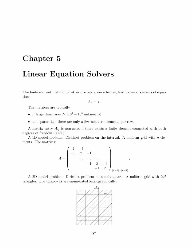
Chapter 5
Linear Equation Solvers
The finite element method, or other discretization schemes, lead to linear systems of equa-tions
Au = f.
The matrices are typically
• of large dimension N (104 − 108 unknowns)
• and sparse, i.e., there are only a few non-zero elements per row.
A matrix entry Aij is non-zero, if there exists a finite element connected with bothdegrees of freedom i and j.
A 1D model problem: Dirichlet problem on the interval. A uniform grid with n ele-ments. The matrix is
A =
2 −1−1 2 −1
. . . . . . . . .
−1 2 −1−1 2
(n−1)×(n−1)
,
A 2D model problem: Dirichlet problem on a unit-square. A uniform grid with 2n2
triangles. The unknowns are enumerated lexicographically:
h
1
n
2 n−1
(n−1)2
87

88 CHAPTER 5. LINEAR EQUATION SOLVERS
The FEM - matrix of dimension N = (n− 1)2 is
A =
D −I−I D −I
. . . . . . . . .
−I D −I−I D
with D =
4 −1−1 4 −1
. . . . . . . . .
−1 4 −1−1 4
(n−1)×(n−1)
,
and the (n− 1)× (n− 1) identity matrix I.
5.1 Direct linear equation solvers
Direct solvers are factorization methods such as LU -decomposition, or Cholesky factoriza-tion. They require in general O(N3) = O(n6) operations, and O(N2) = O(n4) memory. Afast machine can perform about 109 operations per second. This corresponds to
n ∼N time memory10 102 1 ms 80 kB100 104 16 min 800 MB1000 106 30 years 8 TB
A band-matrix of (one-sided) band-width b is a matrix with
Aij = 0 for |i− j| > b
The LU -factorization maintains the band-width. L and U are triangular factors of band-width b. A banded factorization method costs O(Nb2) operations, and O(Nb) memory.For the 1D example, the band-with is 1. Time and memory are O(n). For the 2D example,the band width is O(n). The time complexity is O(n4), the memory complexity is O(n3).
This corresponds to
n time memory10 10 µs 8 kB100 0.1 s 8 MB1000 16 min 8 GB
Block-elimination methods
By splitting the unknowns into two groups, we rewrite the equation Au = f as a blocksystem (
A11 A12
A21 A22
)(u1
u2
)=
(f1
f2
).

5.1. DIRECT LINEAR EQUATION SOLVERS 89
First, expressing u1 from the first row gives
u1 = A−111 (f1 − A12u2),
and the Schur-complement equation to determine u2
(A22 − A21A−111 A12︸ ︷︷ ︸
=:S
)u2 = f2 − A21A−111 f1.
This block-factorization is used in sub-structuring algorithms: Decompose the domain intom×m sub-domains, each one containing 2 n
m× n
mtriangles. Split the unknowns into interior
(I), and coupling (C) unknowns.
m = 2
The interior ones corresponding to different sub-domains have no connection in the matrix.The block matrix is
(AI AICACI AC
)=
AI,1 AIC,1
. . ....
AI,m2 AIC,m2
ACI,1 · · · ACI,m2 AC
Factorizing the block-diagonal interior block AI splits into m2 independent factorizationproblems. If one uses a banded factorization, the costs are
m2( nm
)4
=n4
m2
Computing the Schur complement
S = AC − ACIA−1I AIC = AC −
m2∑i=1
ACI,iA−1I,iAIC,i
is of the same cost. The Schur complement is of size mn, and has band-width n. Thus,the factorization costs O(mn3). The total costs are of order
n4
m2+mn3

90 CHAPTER 5. LINEAR EQUATION SOLVERS
Equilibrating both terms lead to the optimal number of sub-domains m = n1/3, and to theasymptotic costs
n3.33
If a parallel computer is used, the factorization of AI and the computation of Schur com-plements can be performed in parallel.
The hierarchical sub-structuring algorithm, known as nested dissection, eliminates in-terior unknowns hierarchically:
Let n = 2L. On level l, with 1 ≤ l ≤ L, one has 4l sub-domains. Each sub-domain hasO(2L−l) unknowns. The factorization of the inner blocks on level l costs
4l (2L−l)3 = 23L−l
Forming the Schur-complement is of the same cost. The sum over all levels is
L∑l=1
23L−l = 23L
(1
2+
1
4+ . . .
)≈ 23L
The factorization costs are O(n3). Storing the matrices on each level costs
4l (2L−l)2 = 22L.
The total memory is O(L× 22L) = O(n2 log n).This corresponds to
n time memory10 1 µs 3 kB100 1 ms 500 kB1000 1 s 150 MB
A corresponding sparse factorization algorithm for matrices arising from unstructuredmeshes is based on minimum degree ordering. Successively, the unknowns with the leastconnections in the matrix graph are eliminated.
In 2D, a direct method with optimal ordering is very efficient. In 3D, the situation isworse for the direct solver. There holds N = n3, time complexity = O(N2), and memory= O(N1.33).

5.2. ITERATIVE EQUATION SOLVERS 91
5.2 Iterative equation solvers
Iterative equation solvers improve the accuracy of approximative solution by an successiveprocess. This requires in general much less memory, and, depending on the problem andon the method, may be (much) faster.
The Richardson iteration
A simple iterative method is the preconditioned Richardson iteration (also known as simpleiteration, or Picard iteration):
start with arbitrary u0
for k = 0, 1, . . . convergencedk = f − Aukwk = C−1dk
uk+1 = uk + τwk
Here, τ is a damping parameter which may be necessary to ensure convergence. Thematrix C is called a preconditioner. It should fulfill
1. C is a good approximation to A
2. the matrix-vector multiplication w = C−1d should be cheap
A simple choice is C = diag A, the Jacobi preconditioner. The application of C−1 is cheap.The quality of the approximation C ≈ A will be estimated below. The optimal choice forthe first criterion would be C = A. But, of course, w = C−1d is in general not cheap.
Combining the steps, the iteration can be written as
uk+1 = uk + τC−1(f − Auk)
Let u be the solution of the equation Au = f . We are interested in the behavior of theerror uk − u:
uk+1 − u = uk − u+ τC−1(f − Auk)= uk − u+ τC−1(Au− Auk)= (I − τC−1A)(uk − u)
We call the matrix
M = I − τC−1A
the iteration matrix. The error transition can be estimated by
‖uk+1 − u‖ ≤ ‖M‖ ‖uk − u‖.

92 CHAPTER 5. LINEAR EQUATION SOLVERS
The matrix norm is the associated matrix norm to some vector norm. If ρ := ‖M‖ < 1,then the error is reduced. The error after k steps is
‖uk − u‖ ≤ ρk‖u0 − u‖
To reduce the error by a factor ε (e.g., ε = 10−8), one needs
Nits =log ε
log ρ
iterations.We will focus on the symmetric (A = AT ) and positive definite (uTAu > 0 for u 6=
0) case (short: SPD). Then it makes sense to choose symmetric and positive definitepreconditioners C = CT . Eigenvalue decomposition allows a sharp analysis. Pose thegeneralized eigenvalue problem
Az = λCz.
Let (λi, zi) be the set of eigen-pairs. The spectrum is σC−1A = λi. The eigen-vectorszi are normalized to
‖zi‖C = 1
The eigenvalues can are bounded from below and from above by the Rayleigh quotient:
minv
vTAv
vTCv≤ λi ≤ max
v
vTAv
vTCv
The ratio of largest to smallest eigen-value is the relative spectral condition number
κ =λNλ1
We will establish the spectral bounds
γ1 vTCv ≤ vTAv ≤ γ2 v
TCv ∀ v ∈ RN ,
which allow to bound the eigenvalues
λi ∈ [γ1, γ2],
and the condition number κ ≤ γ2
γ1.
A vector v can be expressed in terms of the eigen-vector basis zi as v =∑viei. There
holds
‖v‖2C =
∑v2i
‖v‖2A =
∑λiv
2i

5.2. ITERATIVE EQUATION SOLVERS 93
Lemma 88. The iteration matrix M can be bounded in A-norm and in C-norm:
‖M‖A ≤ supλ∈[γ1,γ2]
|1− τλ|
‖M‖C ≤ supλ∈[γ1,γ2]
|1− τλ|
Proof: Express v =∑vizi. Then
Mv = (I − τC−1A)v =∑
vi(I − τC−1A)zi =∑
vi(1− τλi)zi
The norm is
‖Mv‖2A =
∑λiv
2i (1− τλi)2
≤ supi
(1− τλi)2∑
λiv2i
≤ supλ∈[γ1,γ2]
(1− τλ)2 ‖v‖2A
and thus
‖M‖A = supv∈Rn
‖Mv‖A‖v‖A
≤ supλ∈[γ1,γ2]
|1− τλ|.
The proof is equivalent for ‖M‖C . 2
1−τγ
γ
1−τγ
1−τγ
γ
γ2
1
21
1
The optimal choice of the relaxation parameter τ is such that
1− τγ1 = −(1− τγ2),
i.e.,
τ =2
γ1 + γ2
The convergence factor is
1− τγ1 =γ2 − γ1
γ2 + γ1
.
Assume we knew sharp spectral bounds γ1 = λ1 and γ2 = λN . Then the convergence factoris
‖M‖ =κ− 1
κ+ 1≈ 1− 2
κ

94 CHAPTER 5. LINEAR EQUATION SOLVERS
The number of iterations to reduce the error by a factor ε is
Nits =log ε
log ρ≈ log ε
−2/κ= log ε−1 κ
2
Take the 1D stiffness matrix of dimension N ×N :
A =
2 −1−1 2 −1
. . . . . . . . .
−1 2 −1−1 2
,
and the trivial preconditioner C = I. The eigen-vectors zi and eigen-values λi are
zi =
(sin
ijπ
N + 1
)j=1,...N
λi = 2− 2 cos(iπ
N + 1)
The extremal eigenvalues are
λ1 = 2− 2 cos(π
N + 1) ≈ π2
N2
λN = 2− 2 cos(Nπ
N + 1≈ 4− π2
N2.
The optimal damping is
τ =2
λ1 + λN=
1
2,
and the convergence factor is
‖M‖ ≈ 1− 2λ1
λN≈ 1− 2π2
N2
The number of iterations isNits ' log ε−1N2
For the 2D model problem with N = (n− 1)2, the condition number behaves like
κ ' n2.
The costs to achieve a relative accuracy ε are
Nits × Costs-per-iteration ' log ε−1n2N ' log ε−1n4
The costs per digit are comparable to the band-factorization. The memory requirement isoptimal O(N).

5.2. ITERATIVE EQUATION SOLVERS 95
The gradient method
It is not always feasible to find the optimal relaxation parameter τ a priori. The gradientmethod is a modification to the Richardson method to find automatically the optimalrelaxation parameter τ :
The first steps are identic:
dk = f − Auk wk = C−1dk
Now, perform the updateuk+1 = uk + τwk
such that the error is minimal in energy norm:
Find τ such that ‖u− uk+1‖A = min!
Although the error cannot be computed, this minimization is possible:
‖u− uk+1‖2A = ‖u− uk − τwk‖2
A
= (u− uk)TA(u− uk)− 2τ(u− uk)TAwk + τ 2(wk)TAwk
This is a convex function in τ . It takes its minimum at
0 = 2(u− uk)TAwk + 2τopt(wk)TAwk,
i.e.,
τopt =wkA(u− uk)(wk)TAwk
=wkdk
(wk)TAwk
Since the gradient method gives optimal error reduction in energy norm, its convergencerate can be estimated by the Richardson iteration with optimal choice of the relaxationparameter:
‖u− uk+1‖A ≤κ− 1
κ+ 1‖u− uk‖A
The Chebyshev method
We have found the optimal choice of the relaxation parameter for one step of the iteration.If we perform m iterations, the overall rate of convergence can be improved by choosingvariable relaxation parameters τ1, . . . τm.
The m-step iteration matrix is
M = Mm . . .M2M1 = (I − τmC−1A) . . . (I − τ1C−1A).
By diagonalization, the A-norm and C-norm are bounded by
‖M‖ ≤ maxλ∈[γ1,γN ]
|(1− τ1λ) . . . (1− τmλ)|
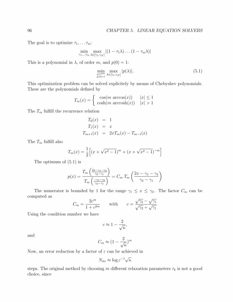
96 CHAPTER 5. LINEAR EQUATION SOLVERS
The goal is to optimize τ1, . . . τm:
minτ1,...τm
maxλ∈[γ1,γN ]
|(1− τ1λ) . . . (1− τmλ)|
This is a polynomial in λ, of order m, and p(0) = 1:
minp∈Pmp(0)=1
maxλ∈[γ1,γN ]
|p(λ)|. (5.1)
This optimization problem can be solved explicitely by means of Chebyshev polynomials.These are the polynomials defined by
Tm(x) =
cos(m arccos(x)) |x| ≤ 1
cosh(m arccosh(x)) |x| > 1
The Tm fulfill the recurrence relation
T0(x) = 1
T1(x) = x
Tm+1(x) = 2xTm(x)− Tm−1(x)
The Tm fulfill also
Tm(x) =1
2
[(x+
√x2 − 1)m + (x+
√x2 − 1)−m
]The optimum of (5.1) is
p(x) =Tm
(2x−γ1−γ2
γ2−γ1
)Tm
(−γ1−γ2
γ2−γ1
) = Cm Tm
(2x− γ1 − γ2
γ2 − γ1
)The numerator is bounded by 1 for the range γ1 ≤ x ≤ γ2. The factor Cm can be
computed as
Cm =2cm
1 + c2mwith c =
√γ2 −
√γ1√
γ2 +√γ1
Using the condition number we have
c ≈ 1− 2√κ,
and
Cm ≈ (1− 2√κ
)m
Now, an error reduction by a factor of ε can be achieved in
Nits ≈ log ε−1√κ
steps. The original method by choosing m different relaxation parameters τk is not a goodchoice, since

5.2. ITERATIVE EQUATION SOLVERS 97
• it is not numerically stable
• one has to know a priori the number of iterations
The recurrence relation for the Chebyshev polynomials leads to a practicable iterativemethod called Chebyshev iteration.
The conjugate gradient method
The conjugate gradient algorithm automatically finds the optimal relaxation parametersfor the best k-step approximation.
Let p0, p1, . . . be a finite sequence of A-orthogonal vectos, and set
Vk = spanp0, . . . pk−1
We want to approximate the solution u in the linear manifold u0 + Vk:
minv∈u0+Vk
‖u− v‖A
We represent uk as
uk = u0 +k−1∑l=0
αlpl
The optimality criteria are
0 = (u− uk, pj)A = (u− u0 −k−1∑l=0
αlpl, pj)A 0 ≤ j < k.
The coefficients αl follow from the A-orthogonality:
αl =(u− u0)TApl
pTl Apl=
(f − Au0)TplpTl Apl
The αl are computable, since the A-inner product was chosen. The best approximationscan be computed recursively:
uk+1 = uk + αkpk
Since uk − u0 ∈ Vk, and pk⊥AVk, there holds
αk =(f − Auk)Tpk
pTkApk.
Any k-step simple iteration approximates the solution uk in the manifold
u0 +Kk(d0)
with the Krylov space
Kk(d0) = C−1d0, C−1AC−1d0, . . . , C
−1(AC−1)k−1d0.
Here, d0 = f −Au0 is the initial residual. The conjugate gradient method computes anA-orthogonal basis of the Krylov-space. The term conjugate is equivalent to A-orthogonal.

98 CHAPTER 5. LINEAR EQUATION SOLVERS
Conjugate Gradient Algorithm:Choose u0, compute d0 = f − Au0, set p0 = C−1d0.for k = 0, 1, 2, . . . compute
αk =dTk pkpTkApk
uk+1 = uk + αk pk
dk+1 = dk − αk Apk
βk = −dTk+1C
−1Apk
pTkApk
pk+1 = C−1dk+1 + βkpk
Remark 89. In exact arithmetic, the conjugate gradient algorithm terminates at a finitenumber of steps k ≤ N .
Theorem 90. The conjugate gradient algorithm fulfills for k ≤ k
1. The sequence pk is A-orthogonal. It spans the Krylov-space Kk(d0)
2. The uk minimizesmin
v∈u0+Kk(d0)‖u− v‖A
3. There holds the orthogonality
dTk pl = 0 ∀ l < k
Proof: Per induction in k. We assume
pTkApl = 0 ∀ l < k
dTk pl = 0 ∀ l < k
This is obvious for k = 0. We prove the property for k + 1: For l < k there holds
dTk+1pl = (dk − αkApk)Tpl = dTk pl − αkpTkApl = 0
per induction. For l = k there is
dTk+1pk = (dk − αkApk)Tpk = dTk pk −dTk pkpTkApk
pTkApk = 0.
Next, prove the A-orthogonality of the pk. For l < k we have
(pk+1, pl)A = (C−1dk+1 + βkpk, pl)A
= dTk+1C−1Apl

5.2. ITERATIVE EQUATION SOLVERS 99
There is
C−1Apl ∈ spanp0, . . . pk,
and dTk+1pj = 0 for j ≤ k. For l = k there is
(pk+1, pk)A = (C−1dk+1 + βkpk, pk)A
= (C−1dk+1, pk)A −dTk+1C
−1Apk
pTkApkpTkApk = 0
2
The coefficients αk and βk should be computed by the equivalent, and numerically morestable expressions
αk =dTkC
−1dkpTkApk
βk =dTk+1C
−1dk+1
dTkC−1dk
.
Theorem 91. The conjugate gradient iteration converges with the rate
‖u− uk‖A ≤(√
κ− 1√κ+ 1
)kProof: The conjugate gradient gives the best approximation in the Krylov space. Thus,
it can be bounded by the Chebyshev method leading to that rate.
The conjugate gradient iteration is stopped as soon as a convergence criterion is fulfilled.Ideally, on wants to reduce the error in the energy norm by a factor ε:
‖u− uk‖A ≤ ε ‖u− u0‖A
But, the energy error cannot be computed. We rewrite
‖u− uk‖2A = ‖A−1(f − Auk)‖2
A = ‖A−1dk‖2A = dTkA
−1dk
If C is a good approxiamtion to A, then also C−1 is one to A−1. The error can beapproximated by
dTkC−1dk.
This scalar is needed in the conjugate gradient iteration, nevertheless.
For solving the 2D model problem with C = I, the time complexity is
log ε−1N√κ = log ε−1 n3
The costs for one digit are comparable to the recursive sub-structuring algorithm. In 3D,the conjugate gradient method has better time complexity.

100 CHAPTER 5. LINEAR EQUATION SOLVERS
5.3 Preconditioning
In the following, let the symmetric and positive definite matrix A arise from the finiteelement discretization of the H1-elliptic and continuous bilinear-form A(., .). We constructpreconditioners C such that the preconditioning action
w = C−1 × d
is efficiently computable, and estimate the spectral bounds
γ1 uTCu ≤ uTAu ≤ γ2 u
TCu ∀u ∈ RN
The analysis of the preconditioner is performed in the finite element framework. Forthis, define the Galerkin isomorphism
G : RN → Vh : u→ u =∑
uiϕi,
where ϕi are the fe besis functions. Its dual is
G∗ : V ∗h → RN : d(·)→ (d(ϕi))i=1,...,N .
To distinguish vectors and the corresponding finite element functions, we write vectorsu ∈ RN with underlines (when necessary).
The evaluation of the quadratic form is
uTAu = A(Gu,Gu) ' ‖Gu‖2H1
The Jacobi Preconditioner
The Jacobi preconditioner C isC = diagA.
The preconditioning action is written as
C−1 × d =N∑i=1
ei(eTi Aei)
−1eTi d
Here, ei is the ith unit-vector. Thus, eTi Aei gives the ith diagonal element Aii of the matrix,which is
Aii = A(ϕi, ϕi) ' ‖ϕi‖2H1 .
The quadratic form generated by the preconditioner is
uTCu =N∑i=1
u2i ‖ϕi‖2
A 'N∑i=1
u2i ‖ϕi‖2
H1

5.3. PRECONDITIONING 101
Theorem 92. Let h be the minimal mesh-size of a shape-regular triangulation. Then thereholds
h2 uTCu uTAu uTCu (5.2)
Proof: We start to prove the right inequality
uTAu = ‖∑i
uiϕi‖2A uTCu =
∑i
u2i ‖ϕi‖2
A.
We define the interaction matrix O with entries
Oij =
1 A(ϕi, ϕj) 6= 00 else
On a shape regular mesh, only a (small) finite number of basis functions have overlappingsupport. Thus, O has a small number of entries 1 per row. There holds
‖∑i
uiϕi‖2A =
∑i
∑j
uiujA(ϕi, ϕj)
=∑i
∑j
uiujOijA(ϕi, ϕj)
≤∑i
∑j
(ui‖ϕi‖A)Oij(uj‖ϕj‖A)
≤ ρ(O)∑i
(ui‖ϕi‖A)2
= ρ(O)uTCu.
The spectral radius ρ(O) = maxx∈RNxTOx‖x‖2 is bounded by the (small) finite row-sum norm
of O.The other estimate is proven element by element. Note that
uTAu ' ‖u‖2H1(Ω) =
∑T
‖∑i
uiϕi‖2H1(T )
anduTCu '
∑i
‖uiϕi‖2H1(Ω) =
∑T
∑i
‖uiϕi‖2H1(T ).
We prove the inequality for each individual element. The triangle T has diameter hT . OnT , we expand u in terms of the element shape functions ϕα, namely u|T =
∑3α=1 uαϕα.
We transform to the reference element T :
‖∑α
uαϕα‖2H1(T ) = ‖
∑α
uαϕα‖2L2(T ) + ‖∇
∑α
uαϕα‖2L2(T )
' h2T ‖∑α
uαϕα‖2L2(T )
+ ‖∇∑α
uαϕα‖2L2(T )
≥ h2T ‖∑α
uαϕα‖2L2(T )

102 CHAPTER 5. LINEAR EQUATION SOLVERS
and ∑α
‖uαϕα‖2H1(T ) =
∑α
‖uαϕα‖2L2(T ) +
∑α
‖∇uαϕα‖2L2(T )
' h2T
∑α
‖uαϕα‖2L2(T )
+∑α
‖∇uαϕα‖2L2(T )
∑α
‖uαϕα‖2L2(T )
Both, (u)α → ‖∑
α uαϕα‖L2(T ) and u→∑
α ‖uαϕα‖2L2(T )
1/2
are norms on R3. Since all
norms in R3 are equivalent, we have∑α
‖uαϕα‖2H1(T ) h−2
T ‖∑α
uαϕα‖2H1(T ). (5.3)
By summing over all elements and choosing h = minhT , we have proven the left inequalityof (5.2). 2
Remark: Inequality (5.3) is sharp. To prove this, choose uα = 1.
Block-Jacobi preconditioners
Instead of choosing the diagonal, one can choose a block-diagonal of A, e.g.,
• In the case of systems of PDEs, choose blocks consisting of all degrees of freedomsitting in one vertex. E.g., mechanical deformations (ux, uy, uz).
• For high order elements, choose blocks consisting of all degrees of freedom associatedto the edges (faces, inner) of the elements.
• On anisotropic tensor product meshes, choose blocks consisting of unknowns in theshort direction
• Domain decomposition methods: Choose blocks consisting of the unknowns in asub-domain
Decompose the unknowns into M blocks, the block i has dimension Ni. Define therectangular embedding matrices
Ei ∈ RN×Ni i = 1, . . . ,M.
Ei consists of Ni unit vectors corresponding to the unknowns in the block i. Each u ∈ RN
can be uniquely written as
u =M∑i=1
Eiui with ui ∈ RNi

5.3. PRECONDITIONING 103
The diagonal blocks areAi = ET
i AEi i = 1, . . . ,M.
The block Jacobi preconditioner is
C−1 × d =M∑i=1
EiA−1i ET
i d
The quadratic form induced by C can be written as
uTCu =∑i
uTi Aiui =∑i
‖GEiui‖2A
where u =∑Eiui.
Example: Discretize the unit interval I = (0, 1) into n elements of approximate sizeh ' 1/n. Split the unknowns into two blocks, the left half and the right half, and definethe corresponding block-Jacobi preconditioner.
SetI = I1 ∪ Tn/2 ∪ I2,
with I1 = (0, xn/2), Tn/2 = [xn/2, xn/2+1], and I2 = (xn/2+1, 1). Decompose
u = E1u1 + E2u2.
The corresponding finite element functions are ui = GEiui. There holds
u1(x) =
Gu(x) x ∈ I1
linear x ∈ T0 x ∈ I2
,
and u2 vice versa. The quadratic form is
uTCu =∑i
uiAiui =∑i
‖GEiui‖2A
Evaluation gives
‖u1‖2A = ‖u1‖2
H1(I1) + ‖u1‖2H1(T )
' ‖u1‖2H1(I1) + h−1|u(xn/2)|2
‖u‖2H1(I) + h−1‖u‖2
H1(I) (trace theorem)
' h−1 ‖u‖2A,
and thusuTCu =
∑i
‖ui‖2A h−1‖u‖2
A ' h−1uTAu.
The situation is the same in Rd.Exercise: Sub-divide the interval I intoM sub-domains of approximative sizeH ≈ 1/M .
What are the sprectral bounds of the block-Jacobi preconditioner ?

104 CHAPTER 5. LINEAR EQUATION SOLVERS
Additive Schwarz preconditioners
The next generalization is an overlapping block Jacobi preconditioner. For i = 1, . . . ,Mlet Ei ∈ RN×Ni be rectangular matrices such that each u ∈ RN can be (not necessarilyuniquely) written as
u =M∑i=1
Eiui with ui ∈ RNi
Again, the overlapping block-Jacobi preconditioning action is
C−1 × d =M∑i=1
EiA−1i ET
i d
Example: Choose the unit-interval problem from above. The block 1 contains all nodes in(0, 3/4), and the block 2 contains nodes in (1/4, 1). The blocks overlap, the decompositionis not unique.
The columns of the matrices Ei are not necessarily unit-vectors, but are linearly in-dependent. In this general setting, the preconditioner is called Additive Schwarz precon-ditioner. The following lemma gives a useful representation of the quadratic form. Itwas proven in similar forms by many authors (Nepomnyaschikh, Lions, Dryja+Widlund,Zhang, Xu, Oswald, Griebel, ...) and is called also Lemma of many fathers, or Lions’Lemma:
Lemma 93 (Additive Schwarz lemma). There holds
uTCu = infui∈R
Ni
u=∑Eiui
M∑i=1
uTi Aiui
Proof: The right hand side is a constrained minimization problem of a convex function.The feasible set is non-empty, the CMP has a unique solution. It is solved by means ofLagrange multipliers. Define the Lagrange-function (with Lagrange multipliers λ ∈ RN):
L((ui), λ) =∑
uTi Aui + λT (u−∑
Eiui).
Its stationary point (a saddle point) is the solution of the CMP:
0 = ∇uiL((ui), λ) = 2Aiui + ETi λ
0 = ∇λL((ui), λ) = u−∑
Eiui
The first line gives
ui =1
2A−1i ET
i λ.
Use it in the second line to obtain
0 = u− 1
2
∑EiA
−1i Eiλ = u− 1
2C−1λ,

5.3. PRECONDITIONING 105
i.e., λ = 2Cu, andui = A−1
i ETi Cu.
The minimal value is ∑uTi Aiui =
∑uTCEiA
−1i AiA
−1i ET
i Cu
=∑
uTCEiA−1i ET
i Cu
= uTCC−1Cu = uTCu
2
Next, we rewrite the additive Schwarz iteration matrix
I − τC−1A = I − τM∑i=1
EiA−1i ET
i A
in the fe framework. LetVi = GEiRNi ⊂ Vh
be the sub-space corresponding to the range of Ei, and define the A-orthogonal projection
Pi : Vh → Vi : A(Piu, vi) = A(u, vi) ∀ vi ∈ ViLemma 94. Set u = Gu, the application of the iteration matrix is u = (I− τC−1A)u, andset u = Gu. Then there holds
u =
(I − τ
M∑i=1
Pi
)u.
Proof: Let wi = A−1i ET
i Au. Then
u = u− τGEiwi.
There holds wi := GEiwi ∈ Vi, and
A(GEiwi, GEivi) = vTi ETi AEiwi
= vTi Aiwi = vTi ETi Au
= A(Gu,GEivi) ∀ vi ∈ RNi ,
i.e., wi = Piu. 2
The additive Schwarz preconditioner is defined by the space splitting
V =M∑i=1
Vi
If the spaces Vi are A-orthogonal, then∑
i Pi = I, and (with τ = 1), and the iterationmatrix is M = 0.
The reformulation of the additive Schwarz lemma 93 in the finite element framework is

106 CHAPTER 5. LINEAR EQUATION SOLVERS
Lemma 95 (Additive Schwarz lemma). Let u = Gu. There holds
uTCu = infui∈Viu=
∑ui
M∑i=1
‖ui‖2A
Example: Let
A(u, v) =
∫ 1
0
u′v′ + ε
∫uv dx
with 0 ≤ ε 1. The bilinear-form is H1-elliptic and continuous, but the bounds dependon the parameter ε. Let CJ be the Jacobi preconditioner. The proof of Theorem 92 showsthat
εh2uTCJu uTAu uTCJu.
The non-robust lower bound is sharp: Take u = (1, . . . , 1)T .The solution is to add the additional sub-space
V0 = span1 = GE0R1
to the AS preconditioner (with E0 ∈ RN×1 consisting of 1-entries). The preconditioningaction is
C−1 × d = diagA−1d+ E0(ET0 AE0)−1ET
0 d.
The spectral bounds are robust in ε:
h2uTCu uTAu uTCu,
namely
uTCu = infui∈Vi
u=∑M
0 ui
M∑i=0
‖ui‖2A
= infu0∈V0
‖u0‖2A + inf
ui∈Viu−u0=
∑M1 ui
M∑i=1
‖ui‖2A
inf
u0∈V0
‖u0‖2A + h−2‖u− u0‖2
H1
The last step was the result of the Jacobi preconditioner applied to (u, v)H1 . Finally, we
choose u0 =∫ 1
0u dx to obtain
uTCu ‖u0‖2A + h−2‖u− u0‖2
H1
ε ‖u0‖2L2
+ h−2‖∇(u− u0)‖2L2
ε ‖u‖2L2
+ h−2‖∇u‖2L2
= h−2 ‖u‖2A

5.3. PRECONDITIONING 107
Overlapping domain decomposition preconditioning
Let Ω = ∪Mi=1Ωi be a decomposition of Ω into M sub-domains of diameter H. Let Ωi besuch that
Ωi ⊂ Ωi dist∂Ωi \ ∂Ω, ∂Ωi H,
and only a small number of Ωi are overlapping. Choose a finite element mesh of meshsize h ≤ H, and the finite element space is Vh. The overlapping domain decompositionpreconditioner is the additive Schwarz preconditioner defined by the sub-space splitting
Vh =∑
Vi with Vi = Vh ∩H10 (Ωi).
The bilinear-form A(., .) is H1-elliptic and continuous. The implementation takes the sub-
matrices of A with nodes inside the enlarged sub-domains Ωi.
Lemma 96. The overlapping domain decomposition preconditioner fulfills the spectral es-timates
H2uTCu uAu uTCu.
Proof: The upper bound is generic. For the lower bound, we construct an explicitdecomposition u =
∑ui.
There exists a partition of unity ψi such that
0 ≤ ψi ≤ 1, suppψi ⊂ Ωi,M∑i=1
ψi = 1
and
‖∇ψi‖L∞ H−1.
Let Πh : L2 → Vh be a Clement-type quasi-interpolation operator such that Πh is aprojection on Vh, and
‖Πhv‖L2 ‖v‖L2 , and ‖∇Πhv‖L2 ‖∇v‖L2 .
For given u ∈ Vh, we choose the decomposition
ui = Πh(ψiu).
Indeed ui ∈ Vi is a decomposition of u ∈ Vh:∑ui =
∑Πh(ψiu) = Πh
((∑
ψi)u)
= Πhu = u

108 CHAPTER 5. LINEAR EQUATION SOLVERS
The lower bound follows from
uTCu = infu=
∑vi
∑i
‖vi‖2A
≤∑i
‖ui‖2A
∑i
‖ui‖2H1
=∑i
‖Πh(ψiu)‖2H1
∑i
‖ψiu‖2H1
=∑i
‖ψiu‖2
L2(Ωi)+ ‖∇(ψiu)‖2
L2(Ωi)
∑i
‖ψiu‖2
L2(Ωi)+ ‖(∇ψi)u‖2
L2(Ωi)+ ‖ψi∇u‖2
L2(Ωi)
∑i
‖u‖2
L2(Ωi)+H−2‖u‖2
L2(Ωi)+ ‖∇u‖2
L2(Ωi)
‖u‖2
L2(Ω) +H−2 ‖u‖2L2(Ω) + ‖∇u‖2
L2(Ω)
H−2 ‖u‖2A.
2
Overlapping DD preconditioning with coarse grid correction
The local DD preconditioner above gets worse, if the number of sub-domains increases. Inthe limit, if H ' h, the DD preconditioner is comparable to the Jacobi preconditioner.
To overcome this degeneration, we add one more subspace. Let TH be a coarse mesh ofmesh-size H, and Th is the fine mesh generated by sub-division of TH . Let VH be the finiteelement space on TH . The sub-domains of the domain decomposition are of the same sizeas the coarse grid.
The sub-space decomposition is
Vh = VH +M∑i=1
Vi.
Let GH : RNH → VH be the Galerkin isomorphism on the coarse grid, i.e.,
GHuH =
NH∑i=1
uH,iϕHi
The coarse space fulfills VH ⊂ Vh. Thus, every coarse grid basis ϕHi can be written aslinear combination of fine grid basis functions ϕhj :
ϕHi =N∑j=1
EH,jiϕhj .
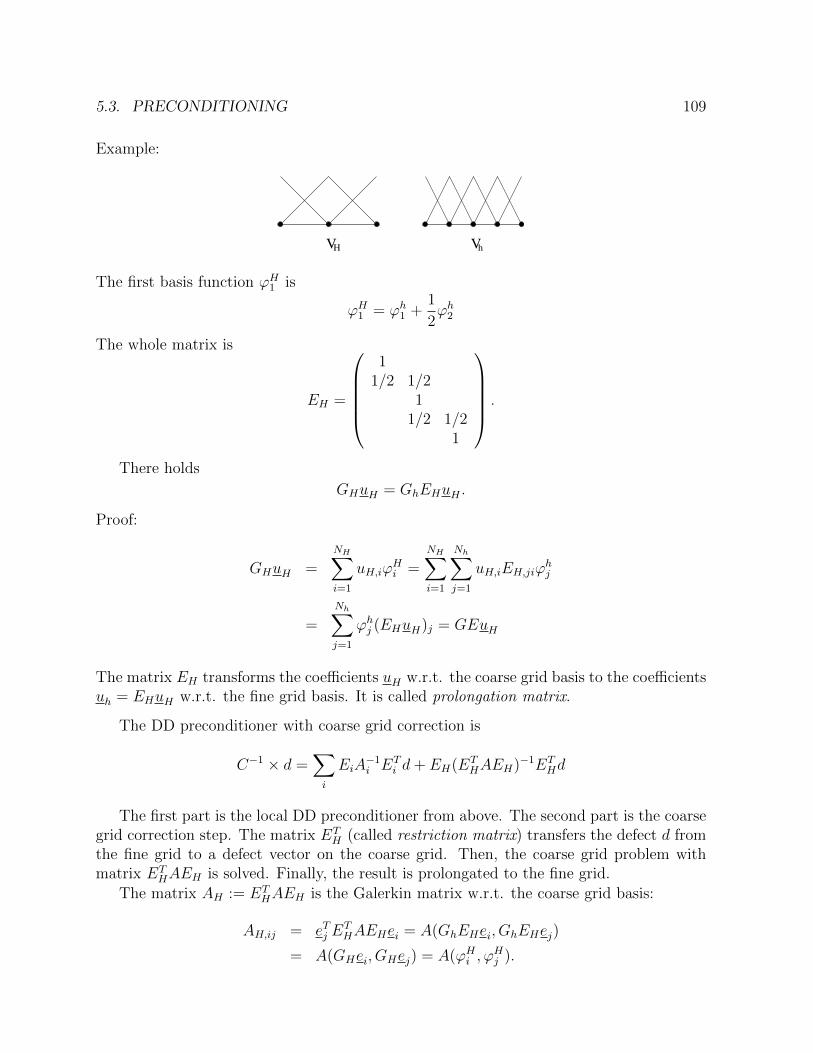
5.3. PRECONDITIONING 109
Example:
H hV V
The first basis function ϕH1 is
ϕH1 = ϕh1 +1
2ϕh2
The whole matrix is
EH =
1
1/2 1/21
1/2 1/21
.
There holds
GHuH = GhEHuH .
Proof:
GHuH =
NH∑i=1
uH,iϕHi =
NH∑i=1
Nh∑j=1
uH,iEH,jiϕhj
=
Nh∑j=1
ϕhj (EHuH)j = GEuH
The matrix EH transforms the coefficients uH w.r.t. the coarse grid basis to the coefficientsuh = EHuH w.r.t. the fine grid basis. It is called prolongation matrix.
The DD preconditioner with coarse grid correction is
C−1 × d =∑i
EiA−1i ET
i d+ EH(ETHAEH)−1ET
Hd
The first part is the local DD preconditioner from above. The second part is the coarsegrid correction step. The matrix ET
H (called restriction matrix) transfers the defect d fromthe fine grid to a defect vector on the coarse grid. Then, the coarse grid problem withmatrix ET
HAEH is solved. Finally, the result is prolongated to the fine grid.
The matrix AH := ETHAEH is the Galerkin matrix w.r.t. the coarse grid basis:
AH,ij = eTj ETHAEHei = A(GhEHei, GhEHej)
= A(GHei, GHej) = A(ϕHi , ϕHj ).

110 CHAPTER 5. LINEAR EQUATION SOLVERS
Theorem 97. The overlapping domain decomposition preconditioner with coarse grid sys-tem fulfills the optimal spectral estimates
uTCu uTAu uTCu.
Proof: The quadratic form generated by the preconditioner is
uTCu = infuH∈VH,ui∈Viu=uH+
∑ui
‖uH‖2A +
M∑i=1
‖ui‖2A.
Again, the upper bound uTAu uTCu follows from the finite overlap of the spacesVH , V1, . . . VM . To prove the lower bound, we come up with an explicit decomposition.We split the minimization into two parts:
uTCu = infuH∈VH
infui∈Vi
u−uH=∑ui
‖uH‖2A +
M∑i=1
‖ui‖2A (5.4)
In the analysis of the DD precondition without coarse grid system we have observed that
infui∈Vi
u−uH=∑ui
M∑i=1
‖ui‖2A H−2‖u− uH‖2
L2+ ‖∇(u− uH)‖2
L2
Using this in (5.4) gives
uTCu infuH∈VH
‖uH‖2
A +H−2 ‖u− uH‖2L2
+ ‖∇(u− uH)‖2L2
inf
uH∈VH
‖∇uH‖2
L2+H−2 ‖u− uH‖2
L2+ ‖∇u‖2
L2
To continue, we introduce a Clement operator ΠH : H1 → VH being continuous in the
H1-semi-norm, and approximating in L2-norm:
‖∇ΠHu‖2L2
+H−2‖u− ΠHu‖2L2 ‖∇u‖2
L2
Choosing now uH := ΠHu in the minimization problem we obtain the result:
uTCu ‖∇ΠHu‖2A +H−2 ‖u− ΠHu‖2
L2+ ‖∇u‖2
L2
‖∇u‖2 ' ‖u‖2A
2
The inverse factorH−2 we have to pay for the local decomposition could be compensatedby the approximation on the coarse grid.
The costs for the setup depend on the underlying direct solver for the coarse gridproblem and the local problems. Let the factorization step have time complexity Nα. Let
5.3. PRECONDITIONING 111
N be the number of unknowns at the fine grid, and M the number of sub-domains. Thenthe costs to factor the coarse grid problem and the M local problems are of order
Mα +M
(N
M
)αEquilibrating both terms gives the optimal choice of number of sub-domains
M = Nα
2α−1 ,
and the asymptotic costs
Nα2
2α−1 .
Example: A Cholesky factorization using bandwidth optimization for 2D problems hastime complexity N2. The optimal choice is M = N2/3, leading to the costs of
N4/3.
Multi-level preconditioners
The preconditioner above uses two grids, the fine one where the equations are solved,and an artificial coarse grid. Instead of two grids, one can use a whole hierarchy of gridsT0, T1, . . . , TL = T . The according finite element spaces are
V0 ⊂ V1 ⊂ . . . ⊂ VL = Vh.
Let El be the prolongation matrix from level l to the finest level L. Define
Al = ETl AEl and Dl = diagAl.
Then, the multi-level preconditioner is
C−1 = E0A−10 ET
0 +L∑l=1
ElD−1l ET
l
The setup, and the application of the preconditioner takes O(N) operations. One canshow that the multi-level preconditioner fulfills optimal spectral bounds
uTCu uTAu uTCu.
An iterative method with multi-level preconditioning solves the matrix equation Au = fof size N with O(N) operations !

112 CHAPTER 5. LINEAR EQUATION SOLVERS
5.4 Analysis of the multi-level preconditioner
We want to solve a finite element system on VL := Vh ⊂ H1. To define the multi-levelpreconditioner C = CL, we use also finite element spaces on coarser meshes T0, T1, . . . TL:
V0 ⊂ V1 ⊂ . . . ⊂ VL
Assume hl ' 2−l. Let ϕl,i : 1 ≤ i ≤ Nl be the hat-basis for Vl, with Nl = dimVl. Let Albe the finite element matrix on Vl.
El ∈ RNl×Nl−1 is the prolongation matrix from level l − 1 to level l.The multi-level preconditioner is defined recursively:
C−10 := A−1
0
C−1l := (diagAl)
−1 + ElC−1l−1E
Tl 1 ≤ l ≤ L.
The computational complexity of one application of C−1L is O(N) operations.
(An extended version of) the Additive Schwarz Lemma allows to rewrite
‖ul‖2Cl
= inful=ul−1+
∑Nli=1
ul,iul−1∈Vl−1,ul,i∈spanϕl,i
‖ul−1‖2Cl−1
+
Nl∑i=1
‖ul,i‖2A
= infu=u0+
∑Ll=1
∑Nli=1 ul,i
∑l
∑i
‖ul,i‖2A + ‖u0‖2
A
Reordering the minimization we obtain
‖u‖2CL
= infu=
∑Ll=0
ulul∈Vl
‖u0‖2A +
L∑l=1
inful=
∑ul,i
Nl∑i=1
‖ul,i‖2A
' infu=
∑Ll=0
ulul∈Vl
‖u0‖2A +
L∑l=1
h−2l ‖ul‖
2L2
Lemma 98 (simple analysis).1
LC A LC
Proof. A LC follows from maximal overlap of spaces and the inverse estimate ‖∇ul‖L2 h−1l ‖ul‖L2 . Let u =
∑Ll=0 ul be an arbitrary decomposition:
‖L∑l=0
ul‖2A ≤ (L+ 1)
L∑l=0
‖ul‖2A L
(‖u0‖2
A +L∑l=1
h−2l ‖ul‖
2L2
).
Since the estimate holds for any decompositon, it also holds for the infimum.

5.4. ANALYSIS OF THE MULTI-LEVEL PRECONDITIONER 113
To show C LA we come up with an explicit decomposition of u ∈ VL. Let Πl : L2 →Vl be a Clement-type operator which is a projection and satisfies
‖Πlu‖H1 + h−1l ‖u− Πlu‖L2 ‖u‖H1 ∀u ∈ H1.
Define
u0 := Π0u
ul := Πlu− Πl−1u 1 ≤ l ≤ L.
Then u =∑L
l=0 ul and
‖u‖2C ‖Π0u‖2
A +L∑l=1
h−2l ‖Πlu− Πl−1u‖2
L2 L ‖u‖2
H1 ≈ ‖u‖2A
We have bound each of the L+ 1 terms by the H1-norm of u, thus the factor L.
Next we show an improved estimate leading to the optimal condition numberκ(C−1A) 1, independent of the number of refinement levels:
Lemma 99. There holdsC A C
Proof. We show A C. Let u =∑L
l=0 ul an arbitrary decomposition. First, we split upthe coarsest level:
‖u‖2A ≤ ‖u0‖2
A + ‖L∑l=1
ul‖2A
Next we show the estimate
A(ul, vk) ≤ 2−|l−k|
2 h−1l ‖ul‖h
−1k ‖vk‖ ∀ul ∈ Vl, vk ∈ Vk
We assume l ≤ k. We perform integration by parts on the level-l triangles, and applyCauchy-Schwarz and scaling techniques:
A(ul, vk) =∑T∈Tl
∫T
∇ul∇vk
≤∑T
∫T
−∆ul︸ ︷︷ ︸=0
vk +
∫∂T
∂ul∂n
vk
≤∑T
∥∥∥∥∂ul∂n
∥∥∥∥∂Tl
‖vk‖∂Tl
≤ h−3/2l ‖ul‖L2 h
−1/2k ‖vk‖L2
=√hk/hl︸ ︷︷ ︸
'2−|k−l|/2
h−1l ‖ul‖L2 h
−1k ‖vk‖L2

114 CHAPTER 5. LINEAR EQUATION SOLVERS
We define the overlap - matrix O ∈ RL×L as
Okl = 2−|k−l|/2.
Then
‖L∑l=1
ul‖2A =
N∑l,k=1
A(ul, uk) ∑l,k
Oklh−1k ‖uk‖L2 h
−1l ‖ul‖L2
≤ ρ(O)L∑l=1
h−2l ‖ul‖
2L2
The spectral radius ρ(O) can be estimated by the row-sum-norm, which is bounded by aconvergent geometric sequence
L∑k=1
2−|k−l|/2 ≤ 2∞∑k=0
√2−k≤ 2
1−√
2.
Since the decomposition was arbitrary, the estimate holds for the minimal decomposition.
Now we show C A. We procede similar as above. Let Πl : L2 → Vl be an Clement-type operator such that
‖Πlu‖L2 ≤ ‖u‖L2 ∀u ∈ L2
‖u− Πlu‖L2 h2l ‖u‖H2 ∀u ∈ H2.
We define u0 = Π0u and ul = Πlu− Πl−1u. We obtain the 2 estimates
h−2l ‖ul‖
2L2 h−2
l ‖u‖2L2,
h−2l ‖ul‖
2L2 h2
l ‖u‖H2 .
The idea of the proof is that H1 is the interpolation space [L2, H2]1/2. We define the
K-functional
K(t, u)2 = infu=u0+u2
u0∈L2,u2∈H2
‖u0‖2
L2+ t2‖u2‖2
H2
.
Combining the 2 estimates above we get
h−2l ‖ul‖
2L2 h−2
l K2(h2l , u)
Thus, the sum over L levels is
L∑l=1
h−2l ‖ul‖
2L2≤
L∑l=1
h−2l K2(h2
l , u) 'L∑l=1
2lK2(2−l, u)

5.4. ANALYSIS OF THE MULTI-LEVEL PRECONDITIONER 115
Next we use that K(s, .) ' K(t, .) for t ≤ s ≤ 2t and replace the sum by an integral, andsubstitute t := 2−l, dt ' −2−ldl = tdl:
L∑l=1
h−2l ‖ul‖
2L2≤
∫ L+1
l=1
2lK2(2−l, u)dl
'∫ 1
2−L−1
t−1K2(t, u)dt
t
∫ ∞
0
t−1K2(t, u)dt
t
= ‖u‖[L2,H2]1/2 ' ‖u‖H1
An intuitive explanation of the proof is that different terms of the sum∑L
l=1 h−2l ‖Πlu−
Πl−1u‖L2 are dominated by different frequency components of u. The squared H1-norm isthe sum over H1-norms of the individual frequency components.

116 CHAPTER 5. LINEAR EQUATION SOLVERS
Chapter 6
Mixed Methods
A mixed method is a variational formulation involving two function spaces, and a bilinear-form of a special saddle point structure. Usually, it is obtained from variational problemswith constraints.
6.1 Weak formulation of Dirichlet boundary condi-
tions
We start with the Poisson problem
−∆u = f in Ω, (6.1)
and boundary conditionsu = uD on ΓD,∂u∂n
= 0 on ΓN .
In contrast to the earlier method, we multiply equation (6.1) with test functions v ∈ H1
(without imposing Dirichlet constraints), and integrate by parts. Using the Neumannboundary conditions, we obtain∫
Ω
∇u∇v dx−∫
ΓD
∂u
∂nv ds =
∫Ω
fv dx
The normal derivative ∂u∂n
is not known on ΓD. We simply call it −λ:
λ := −∂u∂n
To pose the Dirichlet boundary condition, we multiply u = uD by sufficiently many testfunctions, and integrate over ΓD:∫
ΓD
uµ ds =
∫ΓD
uDµ ds ∀µ ∈ ?
117
118 CHAPTER 6. MIXED METHODS
Combining both equations, we get the system of equations: Find u ∈ V = H1(Ω) andλ ∈ Q =? such that∫
Ω∇u · ∇v dx +
∫ΓDvλ ds =
∫fv dx ∀ v ∈ V,∫
ΓDuµ ds =
∫ΓDuDµ ds ∀µ ∈ Q.
(6.2)
A similar formulation can be obtained for interface conditions.
6.2 A Mixed method for the flux
We start from the second order pde
div(a∇u) = f in Ω,
and boundary conditions
u = uD on ΓD
a∂u
∂n= g on ΓN
Next, we introduce the flux variable σ := a∇u to rewrite the equations as: Find u and σsuch that
a−1σ −∇u = 0, (6.3)
div σ = −f, (6.4)
and boundary conditions
u = uD on ΓD
σ · n = g on ΓN .
We want to derive a variational formulation for the system of equations. For that, wemultiply the first equations by vector-valued test functions τ , the second equation by testfunctions v, and integrate:∫
Ω(a−1σ) · τ dx −
∫Ωτ · ∇u dx = 0 ∀ τ∫
Ωdiv σ v dx = −
∫fv dx ∀ v
We would like to have the second term of the first equation of the same structure as thefirst term in the second equation. This can be obtained by integration by parts applied toeither one of them. The interesting case is to integrate by parts in the first line to obtain:∫
Ω
aστ dx+
∫Ω
div τ u dx−∫
ΓD
τn u ds−∫
ΓN
τn u ds = 0.

6.3. ABSTRACT THEORY 119
Here, we make use of the boundary conditions. On the Dirichlet boundary, we knowu = uD, and use that in the equation. The Neumann boundary condition σ · n = g mustbe put into the approximation space, it becomes an essential boundary condition. Thus,it is enough to choose test functions of the sub-space fulfilling τ · n = 0. The problem isnow the following. The space V will be fixed later. Find σ ∈ V, σn = g on ΓN , and u ∈ Qsuch that∫
Ω(a−1σ) · τ dx +
∫Ω
div τ u dx =∫
ΓDuDτn ds ∀ τ, τn = 0 on ΓN∫
Ωdiv σ v dx = −
∫fv dx ∀ v
The derivatives are put onto the flux unknown σ (and its test function τ). We don’t haveto derive the primal unknown u. This will give us better approximation for the fluxes thanfor the scalar. That is one of the reasons to use this mixed method.
6.3 Abstract theory
A mixed variational formulation involves two Hilbert spaces V and Q, bilinear-forms
a(u, v) : V × V → R,b(u, q) : V ×Q→ R,
and continuous linear-forms
f(v) : V → R,g(q) : Q→ R.
The problem is to find u ∈ V and p ∈ Q such that
a(u, v) + b(v, p) = f(v) ∀ v ∈ V,b(u, q) = g(q) ∀ q ∈ Q.
(6.5)
The two examples from above are of this form.
Instead of considering this as a system of equations, one can look at the mixed methodas one variational problem on the product spaces V ×Q. For this, simply add both lines,and search for (u, p) ∈ V ×Q such that
a(u, v) + b(u, q) + b(v, p) = f(v) + g(q) ∀ (v, q) ∈ V ×Q.
Define the big bilinear-form B(., .) : (V ×Q)× (V ×Q)→ R as
B((u, p), (v, q)) = a(u, v) + b(u, q) + b(v, p),
to write the whole system as single variational problem
Find (u, p) ∈ V ×Q : B((u, p), (v, q)) = f(v) + g(q) ∀ (v, q) ∈ V ×Q

120 CHAPTER 6. MIXED METHODS
By the Riesz-representation theorem, we can define operators:
A : V → V : u→ Au : (Au, v)V = a(u, v) ∀ v ∈ VB : V → Q : u→ Bu : (Bu, q)Q = b(u, q) ∀ q ∈ QB∗ : Q→ V : p→ B∗p : (B∗p, v)V = b(v, p) ∀ v ∈ V.
By means of these operators, we can write the mixed variational problem as operatorequation
Au + B∗p = JV f,Bu = JQg.
(6.6)
Here, we used the Riesz-isomorphisms JV : V ∗ → V and JQ : Q∗ → Q.
In the interesting examples, the operator B has a large kernel:
V0 := v : Bv = 0
Lemma 100. Assume that B∗Q is closed in V . Then there holds the V -orthogonal decom-position
V = V0 +B∗Q
Proof: There holds
V0 = v : Bv = 0= v : (Bv, q)Q = 0 ∀ q ∈ Q= v : (v,B∗q)V = 0 ∀ q ∈ Q.
This means, V0 is the V -orthogonal complement to B∗Q. 2
Now, we will give conditions to ensure a unique solution of a mixed problem:
Theorem 101 (Brezzi’s theorem). Assume that a(., .) and b(., .) are continuous bilinear-forms
a(u, v) ≤ α2 ‖u‖V ‖v‖V ∀u, v ∈ V, (6.7)
b(u, q) ≤ β2 ‖u‖V ‖q‖Q ∀u ∈ V, ∀ q ∈ Q. (6.8)
Assume there holds coercivity of a(., .) on the kernel,i.e.,
a(u, u) ≥ α1 ‖u‖2V ∀u ∈ V0, (6.9)
and there holds the LBB (Ladyshenskaja-Babuska-Brezzi) condition
supu∈V
b(u, q)
‖u‖V≥ β1 ‖q‖Q ∀ q ∈ Q. (6.10)
Then, the mixed problem is uniquely solvable. The solution fulfills the stability estimate
‖u‖V + ‖p‖Q ≤ c‖f‖V ∗ + ‖g‖Q∗,
with the constant c depending on α1, α2, β1, β2.

6.3. ABSTRACT THEORY 121
Proof: The big bilinear-form B(., .) is continuous
B((u, p), (v, q)) (‖u‖+ ‖p‖) (‖v‖+ ‖q‖).
We prove that it fulfills the inf − sup condition
infv,q
supu,p
B((u, p), (v, q))
(‖v‖V + ‖q‖Q)(‖u‖V + ‖p‖Q)≥ β.
Then, we use Theorem 33 (by Babuska-Aziz) to conclude continuous solvability.To prove the inf − sup-condition, we choose arbitrary v ∈ V and q ∈ Q. We will
construct u ∈ V and p ∈ Q such that
‖u‖V + ‖p‖Q ‖v‖V + ‖q‖Q
andB((u, p), (v, q)) = ‖v‖2
V + ‖q‖2Q.
First, we use (6.10) to choose u1 ∈ V such that
b(u1, q) = ‖q‖2Q and ‖u1‖V ≤ 2β−1
1 ‖q‖Q.
Next, we solve a problem on the kernel:
Find u0 ∈ V0 : a(u0, w0) = (v, w0)V − a(u1, w0) ∀w0 ∈ V0
Due to assumption (6.9), the left hand side is a coercive bilinear-form on V0. The righthand side is a continuous linear-form. By Lax-Milgram, the problem has a unique solutionfulfilling
‖u0‖V ‖v‖V + ‖u1‖VWe set
u = u0 + u1.
By the Riesz-isomorphism, we define a z ∈ V such that
(z, w)V = (v, w)V − a(u,w) ∀w ∈ V
By construction, it fulfills z⊥V V0. The LBB condition implies
‖p‖Q ≤ β−11 sup
v
b(v, p)
‖v‖V= β−1
1 supv
(v,B∗p)V‖v‖V
= β−11 ‖B∗p‖V ,
and thus B∗Q is closed, and z ∈ B∗Q. Take the p ∈ Q such that
z = B∗p.
It fulfills‖p‖Q ≤ β−1
1 ‖z‖V ‖v‖V + ‖q‖Q

122 CHAPTER 6. MIXED METHODS
Concluding, we have constructed u and p such that
‖u‖V + ‖p‖Q ‖v‖V + ‖q‖Q,
and
B((u, p), (v, q)) = a(u, v) + b(v, p) + b(u, q)
= a(u, v) + (z, v)V + b(u, q)
= a(u, v) + (v, v)V − a(u, v) + b(u, q)
= ‖v‖2V + b(u1, q)
= ‖v‖2V + ‖q‖2
Q.
2
6.4 Analysis of the model problems
Now, we apply the abstract framework to the two model problems.
Weak formulation of Dirichlet boundary conditions
The problem is well posed for the spaces
V = H1(Ω) and Q = H−1/2(ΓD)
Remember, H−1/2(ΓD) is the dual to H1/2(ΓD). The later one is the trace space of H1(Ω),the norm fulfills
‖uD‖H1/2(ΓD) ' infw∈H1
tr w=uD
‖w‖H1(Ω).
The bilinear-forms are
a(u, v) =
∫Ω
∇u∇v dx
b(u, λ) = 〈λ, tr u〉H−1/2×H1/2
To be precise, the integral∫
ΓDλu dx is extended to the duality product 〈λ, u〉. For regular
functions (λ ∈ L2(ΓD)), we can write the L2-inner product.
Theorem 102. The mixed problem (6.2) has a unique solution u ∈ H1(Ω) and λ ∈H−1/2(ΓD).
Proof: The spaces V and Q, and the bilinear-forms a(., .) and b(., .) fulfill the assump-tions of Theorem 101. The kernel space V0 is
V0 = u :
∫ΓD
uµ dx = 0 ∀µ ∈ L2(ΓD) = u : trΓD u = 0

6.4. ANALYSIS OF THE MODEL PROBLEMS 123
The continuity of a(., .) on V is clear. It is not coercive on V , but, due to Friedrichsinequality, it is coercive on V0.
The bilinear-form b(., .) is continuous on V ×Q:
b(u, µ) = 〈µ, tr u〉H−1/2×H1/2 ≤ ‖µ‖H−1/2‖ tr u‖H1/2(ΓD) ‖µ‖Q‖u‖H1 = ‖µ‖Q‖u‖V
The LBB - condition of b(., .) follows more or less from the definition of norms:
‖q‖Q = supu∈H1/2
〈q, u〉‖u‖H1/2
' supu∈H1/2
〈q, u〉inf w∈H1(Ω)
tr w=u
‖w‖H1(Ω)
= supu∈H1/2
supw∈H1(Ω)tr w=u
〈q, u〉‖w‖H1
= supw∈H1
〈q, tr w〉‖w‖H1
= supw∈V
b(w, q)
‖w‖V
Mixed method for the fluxes
This mixed method requires the function space H(div,Ω):
Definition 103. A measurable function g is called the weak divergence of σ on Ω ⊂ Rd ifthere holds ∫
Ω
g ϕ dx = −∫
Ω
σ · ∇ϕdx ∀ϕ ∈ C∞0 (Ω)
The function space H(div) is defined as
H(div,Ω) := σ ∈ [L2(Ω)]d : div σ ∈ L2,
its norms is‖σ‖H(div) =
‖σ‖2
L2+ ‖ div σ‖2
L2
1/2
The mixed method is formulated on the spaces
V = H(div) Q = L2
The bilinear-forms are
a(σ, τ) =
∫a−1στ dx ∀σ, τ ∈ V
b(σ, v) =
∫div σ v dx ∀σ ∈ V, ∀ v ∈ Q
We assume that the symmetric matrix a ∈ Rd×d and its inverse a−1 are bounded.

124 CHAPTER 6. MIXED METHODS
Theorem 104. The mixed problem for the fluxes is well posed.
Proof: We check the conditions of the theorem of Brezzi: The bilinear-forms arebounded, namely
a(σ, τ) =
∫a−1στ dx ≤ ‖a−1‖L∞‖σ‖L2 ‖τ‖L2 ‖σ‖V ‖τ‖V
and
b(σ, v) =
∫div σv dx ≤ ‖ div σ‖L2 ‖v‖L2 ≤ ‖σ‖V ‖v‖Q.
The kernel space V0 = τ : b(τ, v) = 0 ∀ v ∈ Q is
V0 = τ ∈ H(div) : div τ = 0
There holds the kernel-ellipticity of a(., .). Let τ ∈ V0. Then
a(τ, τ) =
∫τTa−1τ dx ≥ inf
x∈Ωλmin(a−1)
∫|τ |2 dx ‖τ‖2
L2= ‖τ‖2
H(div)
We are left to verify the LBB condition
supσ∈H(div)
∫div σ v dx
‖σ‖H(div)
‖v‖L2 ∀ v ∈ L2. (6.11)
For given v ∈ L2, we will construct a flux σ satisfying the inequality. For this, we solvethe artificial Poisson problem −∆ϕ = v with Dirichlet boundary conditions ϕ = 0 on ∂Ω.The solution satisfies ‖∇ϕ‖L2 ‖v‖L2 . Set σ = −∇ϕ. There holds div σ = v. Its norm is
‖σ‖2H(div) = ‖σ‖2
L2+ ‖ div σ‖2
L2= ‖∇ϕ‖2
L2+ ‖v‖2
L2 ‖v‖2
L2.
Using it in (6.11), we get the result∫div σ v dx
‖σ‖H(div)
=
∫v2 dx
‖σ‖H(div)
‖v‖L2 .
The function space H(div)
The mixed formulation has motivated the definition of the function space H(div). Now,we will study some properties of this space. We will also construct finite elements forthe approximation of functions in H(div). In Section 3.3.1, we have investigated traces offunctions in H1. Now, we apply similar techniques to the space H(div). Again, the proofsare based on the density of smooth functions.
For a function in H1, the boundary values are well defined by the trace operator. Fora vector-valued function in H(div), only the normal-component is well defined on theboundary:

6.4. ANALYSIS OF THE MODEL PROBLEMS 125
Theorem 105. There exists a normal-trace operator
trn : H(div)→ H−1/2(∂Ω)
such that for σ ∈ H(div) ∩ [C(Ω)]d it coincides with its normal component
trn σ = σ · n on ∂Ω.
Proof: For smooth functions, the trace operator gives the normal component on theboundary. We have to verify that this operator is bounded as operator from H(div) toH−1/2(∂Ω). Then, by density, we can extend the trace operator to H(div). Let σ ∈H(div) ∩ [C1(Ω)]d:
‖ trn σ‖H−1/2 = supϕ∈H1/2(∂Ω)
∫∂Ωσ · nϕds‖ϕ‖H1/2
' supϕ∈H1(Ω)
∫∂Ωσ · n tr ϕds
‖ϕ‖H1
= supϕ∈H1(Ω)
∫∂Ω
(σ tr ϕ) · n ds‖ϕ‖H1
= supϕ∈H1(Ω)
∫Ω
div(σϕ) dx
‖ϕ‖H1
= supϕ∈H1(Ω)
∫Ω
(div σ)ϕdx+∫
Ωσ · ∇ϕdx
‖ϕ‖H1
≤ supϕ∈H1(Ω)
‖ div σ‖L2 ‖ϕ‖L2 + ‖σ‖L2 ‖∇ϕ‖L2
‖ϕ‖H1
≤‖σ‖2
L2+ ‖ div σ‖2
L2
1/2= ‖σ‖H(div)
2
Lemma 106. There holds integration by parts∫Ω
σ · ∇ϕdx+
∫Ω
(div σ)ϕdx = 〈trn σ, trϕ〉H−1/2×H1/2
for all σ ∈ H(div) and ϕ ∈ H1(Ω).
Proof: By density of smooth functions, and continuity of the trace operators.
Now, let Ω1, . . .ΩM be a non-overlapping partitioning of Ω. In Section 3.3.1, we haveproven that functions which are in H1(Ωi), and which are continuous across the boundariesγij = Ωi ∩ Ωj, are in H1(Ω). A similar property holds for functions in H(div).
Theorem 107. Let σ ∈ [L2(Ω)]d such that
•σ|Ωi ∈ H(div,Ωi)
•trn,i σ|Ωi = − trn,j σ|Ωj on γij.
Then σ ∈ H(div,Ω), and(div σ)|Ωi = div (σ|Ωi).

126 CHAPTER 6. MIXED METHODS
The proof follows the lines of Theorem 46.
We want to compute with functions in H(div). For this, we need finite elements forthis space. The characterization by sub-domains allows the definition of finite elementsub-spaces of H(div). Let T = T be a triangulation of Ω. One family of elements arethe BDM (Brezzi-Douglas-Marini) elements. The space is
Vh = σ ∈ [L2]2 : σ|T ∈ [P k]d, σ · n continuous across edges.
This finite element space is larger than the piece-wise polynomial H1-finite element spaceof the same order. The finite element functions can have non-continuous tangential com-ponents across edges.
The cheapest element for H(div) is the lowest order Raviart-Thomas element RT0.The finite element (T, VT , ψi) is defined by the space of shape functions VT , and linearfunctionals ψi. The element space is
VT =
(ab
)+ c
(x
y
): a, b, c ∈ R
,
the linear functionals are the integrals of the normal components on the three edges of thetriangle
ψi(σ) =
∫ei
σ · n ds i = 1, 2, 3
The three functionals are linearly independent on VT . This means, for each choice ofσ1, σ2, σ3, there exists three unique numbers a, b, c ∈ R such that
σ =(ab
)+ c
(x
y
).
satisfies ψi(σ) = σi.Exercise: Compute the shape functions for the RT0 - reference triangle.
The global finite element functions are defined as follows. Given one value σi for eachedge ei of the triangulation. The corresponding RT0 finite element function σ is definedby
σ|T ∈ VT and
∫ei
σ|T · nei ds = σi
for all edges ei ⊂ T and all triangles T ∈ T .
We have to verify that this construction gives a function in H(div). For each ele-ment, σ|T is a linear polynomial, and thus in H(div, T ). The normal components must becontinuous. By construction, there holds∫
e
σ|T,i · n ds =
∫e
σ|T,j · n ds

6.4. ANALYSIS OF THE MODEL PROBLEMS 127
for the edge e = Ti ∩ Tj. The normal component is continuous since σ · ne is constant onan edge: Points (x, y) on the edge e fulfill xnx + yny is constant. There holds
σ · ne =
[(ab
)+ c
(x
y
)]·(nxny
)= anx + bny + c(xnx + yny) = constant
The global RT0-basis functions ϕRTi are associated to the edges, and satisfy∫ei
ϕRTj · ne ds = δij ∀ i, j = 1, . . . Nedges
By this basis, we can define the RT - interpolation operator
IRTh σ =∑
edges ei
(∫ei
σ · ne ds)ϕRTi
It is a projection on Vh. The interpolation operator preserves the divergence in mean:
Lemma 108. The RT0 - interpolation operator satisfies∫T
div Ihσ dx =
∫T
div σdx
for all triangles T ∈ T .
Let Ph be the L2 projection onto piece-wise constant finite element functions. Thisis: Let Qh = q ∈ L2 : q|T = const ∀T ∈ T . Then Php is defined by Php ∈ Qh and∫
ΩPhp qh dx =
∫ΩPp qh dx ∀ qh ∈ Qh. This is equivalent to Php satisfies Php ∈ Qh and∫
T
Php dx =
∫T
p dx ∀T ∈ T .
The Raviart-Thomas finite elements are piecewise linear. Thus, the divergence is piece-wise constant. From div Ihσ ∈ Qh and Lemma 108 there follows
div Ihσ = Ph div σ.
This relation is known as commuting diagram property:
H(div)div−→ L2yIh yPh
V RTh
div−→ Qh
(6.12)
The analysis of the approximation error is based on the transformation to the referenceelement. For H1 finite elements, interpolation on the element T is equivalent to interpo-lation on the reference element T , i.e., (Ihv) FT = Ih(v FT ). This is not true for theH(div) elements: The transformation F changes the direction of the normal vector. Thus∫eσ · n ds 6=
∫eσ · n ds.
The Piola transformation is the remedy:

128 CHAPTER 6. MIXED METHODS
Definition 109 (Piola Transformation). Let F : T → T be the mapping from the reference
element T to the element T . Let σ ∈ L2(T ). Then, the Piola transformation
σ = Pσ
is defined byσ(F (x)) = (detF ′)−1F ′σ(x).
The Piola transformation satisfies:
Lemma 110. Let σ ∈ H(div, T ), and σ = Pσ. Then there holds
(div σ)(F (x)) = (detF ′)−1 div σ
Let e be an edge of the reference element, and e = F (e). Then∫e
σ · n ds =
∫e
σ · n ds
Proof: Let ϕ ∈ C∞0 (T ), and ϕ(F (x)) = ϕ(x). Then there holds∫T
div σ ϕdx =
∫T
σ · ∇ϕdx
=
∫T
[(detF ′)−1F ′σ
]·[(F ′)−T∇ϕ
](detF ′) dx
=
∫T
σ∇ϕ dx =
∫T
div σ ϕ dx
=
∫T
(detF ′)−1 (div σ)ϕdx.
Since C∞0 is dense in L2(T ), there follows the first claim. To prove the second one, we showthat ∫
e
(σ · n)ϕds =
∫e
(σ · n)ϕ dx
holds for all ϕ ∈ C∞(T ), ϕ = 0 on ∂T \ e. Then, let ϕ→ 1 on the edge e:∫e
(σ · n)ϕds =
∫T
div(σϕ) dx =
∫T
div(σϕ) dx =
∫e
(σ · n)ϕ ds.
2
Lemma 111. The Raviart-Thomas triangle T and the Raviart-Thomas reference triangleare interpolation equivalent:
IRTh Pσ = PIRTh σ
Proof: The element spaces are equivalent, i.e., VT = PVT, and the functionals ψi(σ) =∫eσ · n ds are preserved by the Piola transformation.
6.5. APPROXIMATION OF MIXED SYSTEMS 129
Theorem 112. The Raviart-Thomas interpolation operator satisfies the approximationproperties
‖σ − IRTh σ‖L2(Ω) h ‖∇σ‖L2(Ω)
‖ div σ − div IRTh σ‖L2(Ω) h ‖∇ div σ‖L2(Ω)
Proof: Transformation to the reference element, using that the interpolation preservesconstant polynomials, and the Bramble Hilbert lemma. The estimate for the divergenceuses the commuting diagram property
‖ div(I − IRTh )σ‖L2 = ‖(I − Ph) div σ‖L2 h ‖∇ div σ‖L2
2
6.5 Approximation of mixed systems
We apply a Galerkin-approximation for the mixed system. For this, we choose (finiteelement) sub-spaces Vh ⊂ V and Qh ⊂ Q, and define the Galerkin approximation (uh, ph) ∈Vh ×Qh by
B((uh, ph), (vh, qh)) = f(vh) + g(qh) ∀ vh ∈ Vh ∀ qh ∈ Qh.
Theorem 113. Assume that the finite element spaces fulfill the discrete stability condition
infv∈Vh,q∈Qh
supu∈Vh,p∈Qh
B((u, p), (v, q))
(‖v‖V + ‖q‖)(‖u‖V + ‖p‖Q)≥ β. (6.13)
Then the discretization error is bounded by the best-approximation error
‖u− uh‖V + ‖p− ph‖Q infvh∈Vh,qh∈Qh
‖u− vh‖V + ‖p− qh‖Q
Proof: Theorem 36 applied to the big system B((u, p), (v, q)). 2
The stability on the continuous level V × Q does not imply the discrete stability !Usually, one checks the conditions of Brezzi on the discrete level to prove stability ofB(., .) on the discrete levels. The continuity of a(., .) and b(., .) are inherited from thecontinuous levels. The stability conditions have to be checked separately. The discretetkernel ellipticity
a(vh, vh) ‖vh‖2V ∀ vh ∈ V0h = vh ∈ Vh : b(vh, qh) = 0 ∀ qh ∈ Qh, (6.14)
and the discrete LBB condition
supuh∈Vh
b(uh, qh)
‖uh‖V ‖qh‖Q ∀ qh ∈ Qh. (6.15)

130 CHAPTER 6. MIXED METHODS
The discrete LBB condition is posed for less dual variables qh in Qh ⊂ Q, but the space inthe supremum is also smaller. It does not follow from the LBB condition on the continuouslevels.
There is a canonical technique to derive the discrete LBB condition from the continuousone:
Lemma 114. Assume there exists a quasi-interpolation operator
Πh : V → Vh
which is continuous‖Πhv‖V ‖v‖V ∀ v ∈ V,
and which satisfiesb(Πhv, qh) = b(v, qh) ∀ qh ∈ Qh.
Then, the continuous LBB condition implies the discrete one.
Proof: For all ph ∈ Qh there holds
supvh∈Vh
b(vh, ph)
‖vh‖V≥ sup
v∈V
b(Πhv, ph)
‖Πhv‖V sup
v∈V
b(v, ph)
‖v‖V ‖ph‖Q
2
Approximation of the mixed method for the flux
Choose the pair of finite element spaces, the Raviart Thomas spaces
Vh = v ∈ H(div) : v|T ∈ V RTT ⊂ V = H(div)
and the space of piece-wise constants
Qh = q ∈ L2 : q|T ∈ P 0 ⊂ Q = L2.
Pose the discrete mixed problem: Find (σh, uh) ∈ Vh ×Qh such that∫Ω
(a−1σh) · τh dx +∫
Ωdiv τh uh dx =
∫ΓDuDτn ds ∀ τh ∈ Vh∫
Ωdiv σh vh dx = −
∫fvh dx ∀ vh ∈ Qh.
(6.16)
Lemma 115 (Discrete Stability). The discrete mixed variational problem (6.16) is wellposed.
Proof: By Brezzi’s theorem. Continuity of the bilinear-form and the linear-form followfrom the continuous level. We prove the kernel ellipticity: Since
div Vh ⊂ Qh,

6.5. APPROXIMATION OF MIXED SYSTEMS 131
there holds ∫div σh qh dx = 0 ∀ qh ∈ Qh ⇒ div σh = 0,
and thus V0h ⊂ V0. In this special case, the discrete kernel ellipticity is simple the restrictionof the continuous one to V0h. We are left with the discrete LBB condition. We would liketo apply Lemma 114. The quasi-interpolation operator is the Raviar-Thomas interpolationoperator IRTh . The abstract condition
b(IRTh σ, vh) = b(σ, vh) vh ∈ Qh
reads as ∫T
div IRTh σ dx =
∫T
div σdx,
which was proven in Lemma 108. But, the interpolation operator is not continuous onH(div). The edge-integrals are not well defined on H(div). We have to include the sub-space [H1]d ⊂ H(div). There holds
‖IRTh σ‖H(div) ‖σ‖H1 ∀σ ∈ [H1]d,
and the stronger LBB condition (see Section on Stokes below)
supσ∈[H1]d
(div σ, v)L2
‖σ‖H1
≥ β‖v‖L2 ∀ v ∈ L2.
We follow the proof of Lemma 114: For all vh ∈ Qh there holds
supσh∈Vh
b(σh, vh)
‖σh‖V≥ sup
σ∈[H1]d
(div IRTh σ, vh)
‖IRTh σ‖V sup
σ∈[H1]d
(div σ, vh)
‖σ‖H1
‖vh‖L2 .
Brezzi’s theorem now proves that the discrete problem is well posed, i.e., it fulfills thediscrete inf-sup condition.
2
Theorem 116 (A priori estimate). The mixed finite element methods for the fluxes satisfiesthe error estimates
‖σ − σh‖L2 + ‖ div(σ − σh)‖L2 + ‖u− uh‖L2 h (‖σ‖H1 + ‖u‖H1 + ‖f‖H1) (6.17)
Proof: By discrete stability, one can bound the discretization error by the best approx-imation error
‖σ − σh‖H(div) + ‖u− uh‖L2 infτh∈Vhvh∈Qh
‖σ − τh‖H(div) + ‖u− vh‖L2
.
The best approximation error is bounded by the interpolation error. The first term is(using the commuting diagram property and div σ = f)
infτh∈Vh
‖σ − τh‖L2 + ‖ div(σ − τh)‖L2 ≤ ‖σ−IRTh σ‖L2+‖(I−P 0) div σ‖L2 h (‖σ‖H1 + ‖f‖H1) .

132 CHAPTER 6. MIXED METHODS
The second term is
infvh∈Qh
‖u− vh‖L2 ≤ ‖u− P 0u‖L2 h ‖u‖H1 .
2
The smoothness requirements onto the solution of (6.17) are fulfilled for problems onconvex domains, and smooth (constant) coefficients a. There holds ‖u‖H2 ‖f‖L2 . Sinceσ = a∇u, there follows ‖σ‖H1 ‖f‖L2 . The mixed method requires more smoothnessonto the right hand side data, f ∈ H1. It can be reduced to H1 on sub-domains, what isa realistic assumption. On non-convex domains, u is in general not in H2 (and σ not inH1). Again, weighted Sobolev spaces can be used to prove similar estimates on properlyrefined meshes.
Approximation of the mixed method for Dirichlet boundary conditions
A possibility is to choose continuous and piece-wise linear finite element spaces on thedomain and on the boundary
Vh = v ∈ C(Ω) : v|T ∈ P 1 ∀T,
Qh = µ ∈ C(∂Ω) : µ|E ∈ P 1 ∀E ⊂ ∂Ω.
Theorem 117. The discrete mixed method is well posed.
Proof: Exercises.
6.6 Supplement on mixed methods for the flux : dis-
crete norms, super-convergence and implementa-
tion techniques
6.6.1 Primal and dual mixed formulations
A mixed method for the flux can be posed either in the so called primal form: find σ ∈V = [L2]2, u ∈ H1 with u = uD on ΓD such that∫
Ω(a−1σ) · τ dx −
∫Ωτ · ∇u dx = 0 ∀ τ,
−∫
Ωσ · ∇v dx = −
∫fv dx−
∫ΓNgv ds ∀ v, v = 0 on ΓD,
or in the so called dual mixed form: find σ ∈ V = H(div), u ∈ L2 with σ · n = g on ΓN∫Ω
(a−1σ) · τ dx +∫
Ωdiv τ u dx =
∫ΓDuDτn ds ∀ τ, τn = 0 on ΓN∫
Ωdiv σ v dx = −
∫fv dx ∀ v.

6.6. SUPPLEMENTONMIXEDMETHODS FOR THE FLUX : DISCRETE NORMS, SUPER-CONVERGENCE AND IMPLEMENTATION TECHNIQUES133
Both are formally equivalent: If the solutions are smooth enough for integration by parts,both solutions are the same. In both cases, the big-B bilinear-form is inf−sup stable withrespect to the corresponding norms.
The natural discretization for the primal-mixed formulation uses standard H1-finiteelements of order k for u, and discontinuous L2 elements of order k − 1 for σ. Here,the discrete Brezzi conditions are trivial. The dual one requires Raviart-Thomas (RT)or Brezzi-Douglas-Marini (BDM) elements for σ, and L2 elements for u. This pairingdelivers locally exact conservation (
∫∂Tσn = −
∫Tf). In particular this property makes
the method interesting by itself, but often this scheme is a part of a more complex problem(e.g. Navier-Stokes equations).
Our plan is as follows: We want to use the dual finite element method, but analyzeit in a primal - like setting. Since Qh is no sub-space of H1, we have to use a discretecounterpart of the H1-norm:
‖τ‖2Vh
:= ‖τ‖2L2
‖v‖2Qh
:= ‖v‖2H1,h :=
∑T
‖∇v‖2L2(T ) +
∑E⊂Ω
1h‖[v]‖2
L2(E) +∑E⊂ΓD
1h‖v‖2
L2(E)
The factor 1h
provides correct scaling: If we transform an element patch to the referencepatch, the jump term scales like the H1-semi-norm. This norm is called discrete H1-norm,or DG-norm (as it is essential for Discontinuous Galerkin methods discussed later).
There holds a discrete Friedrichs inequality
‖v‖L2 ‖v‖H1,h.
Theorem 118. The dual-mixed discrete problem satisfies Brezzi’s conditons with respectto L2 and discrete H1-norms.
Proof. The a(., .) bilinear-form is continuous and coercive on (Vh, ‖ · ‖L2). Now we showcontinuity of b(., .) on the finite element spaces. We integrate by parts on the elements,and rearrange boundary terms:
b(σh, vh) =
∫Ω
div σh vh =∑T
∫T
div σh vh
=∑T
−∫T
σh · ∇vh +
∫∂T
σh · n vh
=∑T
−∫T
σh · ∇vh +∑E⊂Ω
∫E
σhnE[v] +∑E⊂ΓD
∫E
σhnEv +∑E⊂ΓN
∫E
σhnE︸ ︷︷ ︸=0
v
The jump term is defined as [v](x) = limt→0+ v(x + tnE) − v(x − tnE). Thus, σhnE[v] isindependent of the direction of the normal vector. Next we apply Cauchy-Schwarz, and

134 CHAPTER 6. MIXED METHODS
use that h‖σh · n‖2L2(E) ‖σh‖L2(T ) for some E ⊂ T (scaling and equivalence of norms on
finite dimensional spaces):
b(σh, vh) ≤∑T
‖σh‖L2(T ) ‖∇vh‖L2(T ) +∑E⊂Ω
h1/2‖σ‖L2(E) h−1/2‖[vh]‖L2(E) +
∑E⊂ΓD
...
‖σh‖L2(Ω)‖vh‖H1,h
The linear-forms are continous with norms h−1/2‖uD‖L2(ΓD) and ‖f‖L2(Ω), respectively.Finally, we show the LBB - condition: Given an vh ∈ Qh, we define σh as follows:
σh · nE = 1h[vh] on E ⊂ Ω
σh · nE = 1hvh on E ⊂ ΓD
σh · nE = 0 on E ⊂ ΓN∫T
σh · q = −∫T
∇vh · q ∀ q ∈ [P k−1]2.
This definition mimics σ = −∇v. This construction is allowed by the definition of Raviart-Thomas finite elements. Thus we get
b(σh, vh) =∑T
−∫σh ∇vh︸︷︷︸∈[Pk−1]2
+∑E⊂Ω
1h‖[vh]‖2
L2(E) +∑E⊂ΓD
1h‖vh‖2
L2(E)
=∑T
∫∇vh · ∇vh +
∑E⊂Ω
1h‖[vh]‖2
L2(E) +∑E⊂ΓD
1h‖vh‖L2(E)
= ‖vh‖2H1,h
By scaling arguments we see that ‖σh‖L2 ‖vh‖H1,h. Thus we got σh such that
b(σh, vh)
‖σh‖L2
‖vh‖H1,h,
and we have constructed the candidate for the LBB condition.
6.6.2 Super-convergence of the scalar
Typically, the discretization error of mixed methods depend on best-approximation errorsin all variables:
‖σ − σh‖L2 + ‖u− uh‖H1,h infτh,vh‖σ − τh‖L2 + ‖u− vh‖H1,h
By the usual Bramble-Hilbert and scaling arguments we see that (using the element-wiseL2-projection Ph):
‖u− Phu‖H1,h hk‖u‖H1+k k ≥ 0.
In the lowest order case (k = 0) we don’t get any convergence !!But, we can show error estimates for σ in terms of approximability for σ only. Further-
more, we can perform a local postprocessing to improve also the scalar variable.

6.6. SUPPLEMENTONMIXEDMETHODS FOR THE FLUX : DISCRETE NORMS, SUPER-CONVERGENCE AND IMPLEMENTATION TECHNIQUES135
Theorem 119. There holds
‖σ − σh‖L2 + ‖Phu− uh‖ ‖σ − Ihσ‖L2 ,
where Ih is the canonical RT interpolation operator satisfying the commuting diagram prop-erty div Ih = Ph div.
Proof. As usual for a priori estimates, we apply stability of the discrete problem, and usethe Galerkin orthogonality:
‖Ihσ − σh‖L2 + ‖Phu− uh‖H1,h supτh,vh
B((Ihσ − σh, Phu− uh), (τh, vh))‖τh‖L2 + ‖vh‖H1,h
(6.18)
= supτh,vh
B((Ihσ − σ, Phu− u), (τh, vh))
‖τh‖L2 + ‖vh‖H1,h
(6.19)
Now we elaborate on the terms of B((Ihσ − σ, Phu − u), (τh, vh)) =∫a−1(Ihσ − σ) · τh +∫
div(Ihσ−σ)vh+∫
div τh(Phu−u): For the first one we use Cauchy-Schwarz, and boundsfor the coefficient a: ∫
a−1(Ihσ − σ) · τh ‖σ − Ihσ‖L2 ‖τh‖L2
For the second one we use the commuting diagram, and orthogonality:∫div(Ihσ − σ)vh =
∫(Ph − Id) div σ︸ ︷︷ ︸
∈Q⊥h
vh︸︷︷︸∈Qh
= 0
For the third one we use that div Vh ⊂ Qh:∫div τh︸ ︷︷ ︸∈Vh
(Phu− u)︸ ︷︷ ︸V ⊥h
Thus, the right hand side of equation (6.19) can be estimated by ‖σ − Ihσ‖L2 . Finally, anapplication of the triangle inequality proves the result.
Remark 120. This technique applies for BDM elements as well as for RT. Both satisfydiv Vh = Qh, and the commuting diagram. For RTk elements, i.e. [P k]2 ⊂ RTk ⊂ [P k+1]2
as well as BDMk elements, i.e. BDMk = [P k]d we get the error estimate
‖σ − Ihσ‖L2 hk+1‖σ‖Hk
with k ≥ 0 for RT and k ≥ 1 for BDM.
Remark 121. The scalar variable shows super-convergence: A filtered error, i.e. Phu−uhis of higer order than the error u− uh itself: One order for RT and two orders for BDM
We can apply a local post-processing to compute the scalar part with higher accuracy:We use the equation σ = a∇u, and the good error estimates for σ and Phu. We setQh := P k+1, and solve a local problem on every element:
minvh∈Qh∫
T vh=∫T vh
‖a∇vh − σh‖2L2(T ),a−1
136 CHAPTER 6. MIXED METHODS
6.6.3 Solution methods for the linear system
The finite element discretization leads to the linear system for the coefficient vectors (calledσ and u again): (
A Bt
B 0
)(σu
)=
(0−f
)This matrix is indefinite, it has dimVh positive and dimQh negative eigenvalues. Thiscauses difficulties for the linear equation solver.
The first possibility is a direct solver, which must (in contrast to positive definitesystems) apply Pivot strategies.
A second possibility is block-elimination: eliminate σ from the first equation. Theregularity of A follows from L2-coercivity of a(., .):
σ = −A−1Btu
and insert it into the second equation:
−BA−1Btu = −f
Thanks to the LBB-condition, B has full rank, and thus the Schur complement matrix isregular. Since B is the discretization of the div-operator, Bt of the negative gradient, andA of a(x)−1I, the equation can be interpreted as a discretization of
div a∇u = −f
This approach is not feasible, since A−1 is not a sparse matrix anymore.One can use extensions of the conjugate gradient (CG) method for symmetric but
indefinit matrices (e.g. MINRES). Here, preconditioners are important. Typically, forblock-systems one uses block-diagonal preconditioners to rewrite the system as(
G−1V 0
0 G−1Q
)(A BT
B 0
)(σu
)=
(G−1V 0
0 G−1Q
)(0−f
)where GV and GQ are approximations to the Gramien matrices in Vh and Qh:
GV,ij = (ϕσi , ϕσj )V and GQ,ij = (ϕui , ϕ
uj )Q
One can either choose the H(div)-L2, or the [L2]2-H1 setting, which leads to different kindof preconditioners. Here, the later one is much simpler. This is a good motivation forconsidering the alternative framework.
6.6.4 Hybridization
Hybridization is a technique to derive a new variational formulation which obtains the samesolution, but its system matrix is positive definit. For this, we break the normal-continuity

6.6. SUPPLEMENTONMIXEDMETHODS FOR THE FLUX : DISCRETE NORMS, SUPER-CONVERGENCE AND IMPLEMENTATION TECHNIQUES137
of the flux functions, and re-inforce it via extra equations. We obtain new variables livingon the element-edges (or faces in 3D).
We start from the first equation a−1σ−∇u = 0, multiply with element-wise discontin-uous test-functions τ , and integrate by parts on the individual elements:∫
Ω
a−1στ +∑T
∫T
u div τ −∫∂T
u τn
= 0
We now introduce the new unknown variable u which is indeed the restriction of u ontothe mesh skeleton u|∪E.
We set V :=∏
T H(div, T ) and Q := L2(Ω) ×∏
E H1/2(E), and pose the so called
hybrid problem: find σ ∈ V and (u, u) ∈ Q such that∫Ω
(a−1σ) · τ dx +∑
T
∫T
div τ u dx +∑
T
∫∂Tu τn = 0 ∀ τ ∈ V∑
T
∫T
div σ v dx = −∫fv dx ∀ v ∈ L2(Ω)∑
T
∫∂Tv σn = 0 ∀ v ∈
∏E H
1/2(E).
The last equation can be rearranged edge by edge:∑E⊂Ω
∫E
[σn] v +∑E⊂∂Ω
∫E
σn v = 0 ∀ v ∈∏E
H1/2(E),
which implies normal-continuity of σ. Dirichlet/Neumann boundary conditions are posednow for the skeleton variable u.
This system is discretized by discontinuous RT/BDM elements for σ, piecewise poly-nomials on elements T for u, and piecewise polynomials on edges for u such that the ordermatches with σ · n.
1. This discrete system is well-posed with respect to the norms ‖σ‖V := ‖σ‖L2 and‖u, u‖2 =
∑T ‖∇u‖2
L2(T ) + 1h‖u− u‖2
∂T . Similar proof as for Theorem 118.
2. The components σh and uh of the solution of the hybrid problem correspond to thesolution of the mixed method.
3. Since the σh is discontinuous across elements, the arising matrix A is block-diagonal.Now it is cheap to form the Schur complement
−BA−1BT(uu
)=
(f
0
)This is now a system with a positive definite matrix for unknowns in the elements andon the edges. Since the matrix block for the element-variables is still block-diagonal,they can be locally eliminated, and only the skeleton variables are remaining. In thelowest order case, the matrix is the same as for the non-conforming P 1 element.

138 CHAPTER 6. MIXED METHODS

Chapter 7
Discontinuous Galerkin Methods
Discontinuous Galerkin (DG) methods approximate the solution with piecewise functions(polynomials), which are discontinuous across element interfaces. Advantages are
• block-diagonal mass matrices which allow cheap explicit time-stepping
• upwind techniques for dominant convection
• coupling of non-matching meshes
• more flexibility for stable mixed methods
DG methods require more unknowns, and also have a denser stiffness matrix. The lastdisadvantage can be overcome by hybrid DG methods (HDG).
7.1 Transport equation
We consider the first order equation
div(bu) = f on Ω,
where b is the given wind, and f is the given source. Boundary conditions are specified
u = uD on Γin,
where the inflow boundary is
Γin = x ∈ ∂Ω : b · n < 0,
and the outflow boundary Γout = ∂Ω \ Γin.The instationary transport equation
∂u
∂t+ div(bu) = f on Ω× (0, T )
139

140 CHAPTER 7. DISCONTINUOUS GALERKIN METHODS
with initial conditions u = u0 for t = 0 can be considered as stationary transport equationin space-time:
divx,t(bu) = f,
where b = (b, 1). The inflow boundary consists now of the lateral boundary Γin×(0, T ) andthe bottom boundary Ω×0, which is an inflow boundary according to (b, 1) ·(0,−1) < 0.
The equation in conservative form leads to a conservation principle. Let V be anarbitrary control volume. From the Gauß theorem we get∫
∂V
b · nu =
∫V
f
The total outflow is in balance with the production inside V .For stability, we assume div b = 0. This is a realistic assumption, since the wind is
often the solution of the incompressible Navier Stokes equation.A variational formulation is ∫
div(bu)v =
∫fv ∀v
If we set v = u, and usediv(bu)u = 1
2div(bu2)
We obtain ∫div(bu)v = 1
2
∫∂Ω
bnu2 =
∫fu
For f = 0 we obtain ∫Γout
|bn|u2 =
∫Γin
|bn|u2.
This inflow-outflow isometrie is a stability argument. For time dependent problems (withbn = 0 on ∂Ω), it ensures the conservation of L2-norm in time.
7.1.1 Solvability
We assume b ∈ L∞ with div b = 0. We consider the problem: find u ∈ V , u = uD on Γinand
B(u, v) = f(v) ∀ v ∈ Wwith
B(u, v) =
∫div(bu)v and f(v) =
∫fv
The space V shall be defined by the (semi)-norm
‖u‖V = ‖b∇u‖L2
Depending on b, it is a norm for u = 0 onΓin. Roughly speaking, if every point in Ωcan be reached by a finite trajectory along b, then ‖u‖L2 ‖u‖V , by Friedrichs inequality.

7.2. DISCONTINUOUS GALERKIN DISCRETIZATION 141
It does not hold if b has vortices. Then ‖ · ‖V is only a semi-norm. Note, for space-timeproblems b cannot have vortices. For theory, we will assume that
‖u‖L2 ‖u‖V ∀u = 0 on Γin
The test space isW = L2
The forms B(., .) and f(.) are continuous. The inf − sup conditions is trivial:
supv
B(u, v)
‖v‖L2
≥︸︷︷︸v:=b∇u
∫(b∇u)2
‖b∇u‖= ‖b∇u‖L2
7.2 Discontinuous Galerkin Discretization
A DG method is a combination of finite volume methods and finite element methods. Westart with a triangulation T. On every element we multiply the equation by a test-function: ∫
T
b∇uv =
∫T
fv ∀ v
We integrate by parts:
−∫T
bu∇v +
∫∂T
bnuv =
∫T
fv
On the element-boundary we replace bnu by its up-wind limit bnuup. On the element inflow
boundary ∂Tin = x ∈ ∂T : bnT < 0, the upwind value is the value from the neighbourelement, while on the element outflow boundary it is the value from the current element T .For elements on the domain inflow boundary, the upwind value is taken as the boundaryvalue uD. For the continuous solution there holds
−∫T
bu∇v +
∫∂T
bnuupv =
∫T
fv
Now we integrate back: ∫T
b∇uv +
∫∂T
bn(uup − u)v =
∫T
fv
On the outflow boundary, the boundary integral cancels out, on the inflow boundary wecan write it as a jump term [u] = uup − u:∫
T
b∇uv +
∫∂Tin
bn[u]v =
∫T
fv
We define the DG bilinear-form
BDG(u, v) =∑T
∫T
b∇uv +
∫∂Tin
bn[u]v
.

142 CHAPTER 7. DISCONTINUOUS GALERKIN METHODS
The true solution is consistent with
BDG(u, v) = f(v) ∀ v piece-wise continuous.
We define DG finite element spaces:
Vh := Wh := v ∈ L2 : v|T ∈ P k
The DG formulation is: find uh ∈ Vh such that
BDG(uh, vh) = f(vh) ∀ vh ∈ Wh
For the discontinuous space, the jump-term is important. If we use continous spaces, thejump-term disappears. The discrete norms are defined as
‖uh‖2Vh
:=∑T
‖b∇u‖2L2(T ) +
∑E
1h‖bn[u]‖2
L2(E)
‖vh‖Wh= ‖vh‖L2
The part with the jump-term mimics the derivative as kind of finite difference term acrossedges.
We prove solvability of the discrete problem by showing a discrete inf − sup condition.But, in general, one order in h is lost due to a mesh-dependent inf − sup constant. Thisfactor shows up in the general error estimate by consistency and stability. It can be avoidedin 1D, and on special meshes.
Theorem 122. There holds the discrete inf − sup condition
supvh
B(uh, vh)
‖vh‖Wh
h ‖uh‖Vh
Proof. We take two different test-functions: v1 = uh and v2 := b · ∇Tu, and combine themproperly. The second test-function would not be possible in the standard C0 finite elementspace.
There holds (dropping sub-scripts h):
B(uh, v1) = B(uh, uh) =∑T
∫T
b∇uu+
∫∂Tin
bn[u]u
=∑T
1
2
∫∂T
bnu2 +
∫∂Tin
bn[u]u
We reorder the terms edge-by-edge. On the edge E we get contributions from twoelements: On the inflow-boundary of the down-wind element we get
12
∫E
bn(ud)2 +
∫E
bn(uu − ud)ud =
∫E
|bn|(
12(ud)2 − uuud
)

7.2. DISCONTINUOUS GALERKIN DISCRETIZATION 143
We used that b · n is negative on the inflow boundary. From the up-wind element we geton its outflow-boundary: ∫
E
12|bn| (uu)2
Summing up, we have the square ∫E
12|bn|(uu − ud)2,
and summing over elements we get the non-negative term
B(uh, uh) = 12
∑E
∫E
|bn|[u]2.
An extra treatment of edges on the whole domain boundary gives that the jump must bereplaced by the function values on ∂u.
We plug in the second test function v2:
B(uh, v2) =∑T
∫T
(b∇u)2 +
∫∂Tin
bn[u] b∇u
We use Young’s inequality to bound the second term from below:
B(uh, v2) ≥∑T
∫T
(b∇u)2 − 1
2γ‖bn[u]‖2
∂L2(Tin) −γ
2‖b∇u‖2
L2(∂Tin)
By the choice γ ' h and a inverse trace inequality (which needs smoothness assumptionsonto b) we can bound the last term by the first one on the right hand. Thus
B(uh, v2) ∑T
∫T
(b∇u)2 −∑E
1
h‖[u]‖2
L2(E),bn
Finally, we set
vh =1
hv1 + v2
to obtain
B(uh, vh) ∑T
∫T
(b∇u)2 +∑E
1
h‖[u]‖2
L2(E),bn ' ‖uh‖2Vh.
But, for this choice we get‖vh‖Wh
h−1‖uh‖Vh ,
and thus the h-dependent inf − sup-constant.
144 CHAPTER 7. DISCONTINUOUS GALERKIN METHODS
7.3 Nitsche’s method for Dirichlet boundary condi-
tions
We build in Dirichlet b.c. in a weak sense. In constrast to a mixed method, we obtain apositive definit matrix.
We consider the equation
−∆u = f and u = uD on ∂Ω.
A diffusion coefficient, or mixed boundary conditions are possible as well. We multiplywith testfunctions, integrate and integrate by parts:∫
Ω
∇u∇v −∫∂nuv =
∫fv ∀ v
We do not restrict test functions to v = 0. To obtain a symmetric bilinear-form, we add aconsistent term∫
Ω
∇u∇v −∫∂Ω
∂nuv −∫∂Ω
∂nvu =
∫fv −
∫∂Ω
∂nvuD ∀ v
Finally, to obtain stability (as proven below), we add the so called stabilization term∫Ω
∇u∇v −∫∂Ω
∂nuv −∫∂Ω
∂nvu+α
h
∫uv =
∫fv −
∫∂Ω
∂nvuD +α
h
∫uDv ∀ v
These are the forms of Nitsche’s method:
A(u, v) =
∫Ω
∇u∇v −∫∂Ω
∂nuv −∫∂Ω
∂nvu+α
h
∫∂Ω
uv
f(v) =
∫Ω
fv −∫∂Ω
∂nvuD +α
h
∫∂Ω
uDv
A(., .) is not defined for u, v ∈ H1, but it requires also well defined normal derivatives.This is satisfied for the flux ∇u ∈ H(div) of the solution, and finite element test functionsv.
We define the Nitsche norm:
‖u‖21,h := ‖∇u‖2
L2+ 1
h‖u‖2
L2(∂Ω)
Lemma 123. If α = O(p2) is chosen sufficiently large, then A(., .) is elliptic on the finiteelement space:
A(uh, uh) ‖uh‖21,h ∀uh ∈ Vh
Proof. On one element there holds the inverse trace inequality
‖uh‖2L2(∂T ) ≤ c
p2
h‖uh‖2
L2∀uh ∈ P p(T )

7.3. NITSCHE’S METHOD FOR DIRICHLET BOUNDARY CONDITIONS 145
The h-factor is shown by transformation to the reference element, the p-factor (polynomialorder) is proven by expansion in terms of orthogonal polynomials. Using the element-wiseestimate for all edges on the domain boundary, we obtain
‖uh‖2L2(∂Ω) ≤ c
p2
h‖u‖2
L2(Ω) (7.1)
Evaluating the bilinear-form, and applying Young’s inequality for the mixed term we get
A(uh, uh) = ‖∇uh‖2L2− 2
∫∂Ω
∂nuu+α
h‖u‖2
L2(∂Ω)
≥ ‖∇uh‖2L2− 1
γ‖n · ∇uh‖2
L2(∂Ω) − γ‖u‖2L2(∂Ω) +
α
h‖u‖2
L2(∂Ω)
The inverse trace inequality applied to ∇uh gives
‖n · ∇uh‖∂Ω ≤ ‖∇uh‖∂Ω ≤ cp2
h‖∇uh‖Ω
By choosing
γ > cp2
hand γ ≤ α
h
we can absorb the negative terms into the positive ones. Therefore it is necessary to choose
α > cp2
For the error analysis we apply the discrete stability and consistency:
‖uh − Ihu‖1,h supvh
A(uh − Ihu, vh)‖vh‖1,h
= supvh
A(u− Ihu, vh)‖vh‖1,h
We cannot argue with continuity of A(., .) on H1 (which is not true), but we can estimatethe interpolation error u− Ihu for all four terms of A(uh − Ihu, vh).
7.3.1 Nitsche’s method for interface conditions
We give now a variational formulation for interface conditions u1 = u2, ∂n1u1 + ∂n2)u2 = 0on the interface γ separating Ω1 and Ω2. Boundary conditions on the outer boundary aretreated as usual. Integration by parts on the sub-domains leads to∫
Ω1
∇u∇v −∫γ
∂n1u1v1 +
∫Ω2
∇u∇v −∫γ
∂n2u2v2 =
∫fv

146 CHAPTER 7. DISCONTINUOUS GALERKIN METHODS
We define the mean value∂n1u = 1
2(∂n1u1 + ∂n2u2)
and jump[v] = v1 − v2.
Using continuity of the normal flux (taking the orientation into account) we get∑i
∫Ωi
∇u∇v −∫γ
∂n1u[v] =
∫fv.
Note that both terms, mean of normal derivative and jump, change sign if we exchangethe enumeration of sub-domains.
We procede as before and add consistent symmetry and stabilization terms:∑i
∫Ωi
∇u∇v −∫γ
∂n1u[v]−∫γ
∂n1v[u] +α
h
∫γ
[u][v] =
∫fv.
The variational formulation is consistent on the solution, and elliptic on Vh, which is provenas before. This approach is an alternative to the mixed method (mortar method), since itleads to positive definite matrices (called also gluing method).
7.4 DG for second order equations
Nitsche’s method for interface conditions can be applied element-by-element. This is the(independently developed) Discontinuous Galerkin (DG) method. Precisely, it’s calledSIP-DG (symmetric interior penalty) DG:
A(u, v) =∑T
∫T
∇u∇v − 12
∫∂T
∂nu[v]− 12
∫∂T
∂nv[u] + αh
∫∂T
[u][v]
(and proper treatment of integrals on the domain boundary). The factor 1
2is coming from
splitting the consistent terms to the two elements on the edge.Convergence analysis similar to Nitsche’s method.Beside the SIP-DG, also different version are in use: The NIP-DG (non-symmetric
interior penalty) DG:
A(u, v) =∑T
∫T
∇u∇v − 12
∫∂T
∂nu[v] + 12
∫∂T
∂nv[u] + αh
∫∂T
[u][v]
The term formerly responsible for symmetry is added with a different sign. The variationalproblem is still consistent on the true solution. The advantage of the NIP-DG is that
A(u, u) =∑T
‖∇u‖2L2(T ) + α
h‖[u]‖2
L2(∂T ,

7.4. DG FOR SECOND ORDER EQUATIONS 147
i.e. A(., .) is elliptic in any case α > 0. The disadvantage is that A(., .) is not consistentfor the dual problem, i.e. the Aubin-Nitsche trick cannot be applied. It is popular forconvection-diffusion problems, where the bi-form is non-symmetric anyway. The IIP-DG(incomplete) skips the third term completely. Advantages are not known to the author.
7.4.1 Hybrid DG
One disadvantage of DG - methods is that the number of degrees of freedom is muchhigher than a continuous Galerkin method on the same mesh. Even worse, the number ofnon-zero entries per row in the system matrix is higher. The second disadvantage can beovercome by hybrid DG methods: One adds additional variables u, v on the inter-elementfacets (edges in 2D, faces in 3D). The derivation is very similar:
∑T
∫T
∇u∇v −∫∂T
∂nuv =∑T
fv ∀ v ∈ P k(T ),∀T
Using continuity of the normal flux, we may add∑
T
∫∂T∂nuv with a single-valued test-
function on the facets:∑T
∫T
∇u∇v −∫∂T
∂nu(v − v) =∑T
fv ∀ v ∈ P k(T ),∀T
Again, we smuggle in consistent terms for symmetry and coercivity:∑T
∫T
∇u∇v−∫∂T
∂nu(v−v)−∫∂T
∂nv(u−u)+α
h
∫∂T
(u−u)(v−v) =∑T
fv ∀ v ∈ P k(T ),∀T
The jump between neighbouring elements is now replaced by the difference of element-values and facet values. The natural norm is
‖u, u‖2 =∑T
‖∇u‖2 + 1h‖u− u‖∂T
The HDG methods allows for static condensation of internal variables which results in aglobal system for the edge-unknowns, only.
The lowest order method uses P 1(T ) and P 1(E), and we get O(h) convergence. Whencomparing with the non-conforming P 1-method, HDG has more unknowns on the edges,but the same order of convergence. The Lehrenfeld-trick is to smuggle in a projector:∑T
∫T
∇u∇v−∫∂T
∂nu(v−v)−∫∂T
∂nv(u−u)+α
h
∫∂T
P k−1(u−u)(v−v) =∑T
fv ∀ v ∈ P k(T ), ∀T
This allows to reduce the order on edges by one, while maintaining the order of convergence.

148 CHAPTER 7. DISCONTINUOUS GALERKIN METHODS
7.4.2 Bassi-Rebay DG
One disadvantage of IP-DG is the necessary penalty term with α sufficiently large. For well-shaped meshes α = 5p2 is usually enough. But, for real problems the element deformationmay become large, and then a fixed α is not feasible. Setting α too large has a negativeeffect for iterative solvers.
An alternative is to replace the penalty term by
‖[u]‖2BR := sup
σh∈[Pk−1]d
([u], n · σh)2L2(∂T )
‖σh‖2L2(T )
It can be implemented by solving a local problem with L2-bilinear-form.In the coercivity proof, the bad term is now estimated as∫
∂T
n · ∇uh [uh] ≤ supσh
∫∂Tn · σh [uh]
‖σh‖‖∇uh‖ ≤ ‖∇uh‖ ‖[u]‖BR
The BR-norm scales like the IP - norm (in h and p), but the (typically unknown) constantin the inverse trace inequality can be avoided.
7.4.3 Matching integration rules
Another method to avoid guessing the sufficiently large α is to use integration rules, suchthe the integration points for the boundary integral are a sub-set of the integration pointsof the volume term. Now, Young’s inegality can be applied for the numerical integrals.The α
hfactor is now replace by the largest relative scaling of weights for the boundary
integrals and volume integrals. The pro is the simplicity, the con is the need of numericalintegration rules which need more points.
7.4.4 (Hybrid) DG for Stokes and Navier-Stokes
DG or HDG methods allow the construction of numercal methods for incompressible flows,which obtain exactly divergence free discrete velocities. We discretize Stokes’s equation asfollows:
Vh = BDMk Qh = P k−1,dc,
and the bilinear-formsa(uh, vh) = aDG(uh, vh)
and
b(uh, qh) =
∫div uh qh.
Since the space Vh is not conforming for H1, the DG - technique is applied. The b(., .)bilinear-form is well defined for the H(div)-conforming finite element space Vh. There holds
div Vh = Qh,

7.4. DG FOR SECOND ORDER EQUATIONS 149
and thus the discrete divergence free condition∫div uhqh = 0 ∀qh
implies
‖ div uh‖2L2
=
∫div uh div uh︸ ︷︷ ︸
∈Qh
= 0.
Hybridizing the method leads to facet variables for the tangential components, only. Thismethod can be applied to the Navier Stokes equations. Here, the exact divergence-freediscrete solution leads to a stable method for the nonlinear transport term (References:Master thesis Christoph Lehrenfeld: HDG for Navier Stokes, h-version LBB, Master thesisPhilip Lederer: p-robust LBB for triangular elements).

150 CHAPTER 7. DISCONTINUOUS GALERKIN METHODS

Chapter 8
Applications
We investigate numerical methods for equations describing real life problems.
8.1 The Navier Stokes equation
The Navier Stokes equation describe the flow of a fluid (such as water or air). The in-compressible Navier Stokes equation models incompressible fluids (such as water). Thestationary N.-St. equation models a solution in steady state (no change in time).
The field variables are the fluid velocity u = (ux, uy, uz), and the pressure p. Conserva-tion of momentum is
−ν∆u+ ρ(u · ∇)u−∇p = f
The first term describes friction of the fluid (ν is called viscosity). The second one arisesfrom conservation of momentum of moving particles. It is called the convective term (ρ isthe density). The source term f models forces, mainly gravity. The incompressibility ofthe fluid is described by
div u = 0.
Different types of boundary conditions onto u and p are possible.
The Navier Stokes equation is nonlinear. In general, no unique solution is guaranteed.The common approach to find a solution is the so called Oseen iteration: Given uk, findthe next iterate (uk+1, pk+1) by solving
−ν∆uk+1 + ρ(uk · ∇)uk+1 −∇pk+1 = f
div uk+1 = 0.
Under reasonable conditions, this Oseen equation is uniquely solvable. Since uk is thesolution of the old step, it satisfies div uk = 0. Furthermore, we assume that the velocityuk is bounded in L∞-norm.
151

152 CHAPTER 8. APPLICATIONS
From now on, we continue to investigate the Oseen equation. Given a vector-fieldw = (wx, wy, wz) ∈ [L∞]3 such that div w = 0. Find u and p such that
−∆u+ (w · ∇)u−∇p = f
div u = 0.
We have removed the viscosity by rescaling the equation. The factor ρ/ν is incorporatedinto the vector-field w.
As usual, we go over to the weak formulation: Find u ∈ V = [H1]3 and p ∈ Q = L2
such that ∫∇u∇v + (w · ∇)u v dx +
∫div v p dx =
∫fv dx ∀ v ∈ V∫
div u q dx = 0 ∀ q ∈ Q. (8.1)
This variational problem is a mixed formulation. It satisfies the conditions of Brezzi:The bilinear forms are
a(u, v) =
∫∇u∇v + (w · ∇)uv dx,
b(u, q) =
∫div u q dx.
Both forms are continuous. The form a(., .) is non-symmetric. In a(., .), the x, y, andz components of u and v are independent. To investigate a(., .), it is enough to considerscalar bilinear-forms. We define the inflow and outflow boundaries
Γi = x ∈ ∂Ω : w · n < 0,Γo = x ∈ ∂Ω : w · n ≥ 0.
If we pose Dirichlet boundary conditions on Γi, then a(., .) is coercive (see example 27, andexercises). The ratio of the continuity bound and the coercivity bound depends on thenorm of the convection w. With increasing w, the problem is getting worse.
The form b(., .) satisfies the LBB condition:
supu∈[H1
0,D]3
∫div u q dx
‖u‖H1
‖q‖L2 ∀ q ∈ L2.
In the case of (partial) Dirichlet boundary conditions (H10,D = u : u = 0 on ΓD),
this condition is very nontrivial to prove. If there are only Dirichlet b.c., one has to useQ = L0
2 = q :∫
Ωq dx = 0.
Under these conditions, Brezzi’s theorem proves a unique solution of the Oseen equa-tion.

8.1. THE NAVIER STOKES EQUATION 153
Finite elements for Navier-Stokes equation
We want to approximate the Oseen equation by a Galerkin method: Find uh ∈ Vh andph ∈ Qh such that∫
∇uh∇vh + (w · ∇)uh vh dx +∫
div vh ph dx =∫fvh dx ∀ vh ∈ Vh∫
div uh qh dx = 0 ∀ qh ∈ Q.(8.2)
To obtain convergence uh → u and ph → p, it is important to choose proper approxi-mation spaces Vh and Qh. Using the simplest elements, namely continuous and piece-wiselinear elements for Vh ⊂ [H1]3, and piece-wise constants for Qh ⊂ L2 does not work. Thediscrete LBB condition is not fulfilled: In 2D, there are asymptotically twice as manytriangles than vertices, i.e., dim Vh ≈ dim Qh, and
∫div uh qh dx = 0 ∀ qh ∈ Qh implies
uh ≈ 0.
The simplest spaces which lead to convergence are the non-conforming P1 element forthe velocities, and piece-wise constant elements for the pressure. The arguments are
• There are unknowns on the edges to construct a Fortin operator satisfying∫e
u · n ds =
∫e
(Ihu) · n ds,
and thus proving the discrete LBB condition.
• The error due to the non-conforming space Vh 6⊂ V is of the same order as theapproximation error (see Section 4.5).
8.1.1 Proving LBB for the Stokes Equation
Stability of the continuous equation
We consider Stokes equation: find u ∈ [H10 ]d and p ∈ L0
2 such that∫∇u · ∇v +
∫div v p =
∫fv ∀ v ∈ [H1
0 ]d∫div u q = 0 ∀ q ∈ L0
2.(8.3)
Solvability follows from Brezzi’s theorem. The only non-trivial part is the LBB condition:
supv∈[H1
0 ]d
∫div v p
‖v‖H1
≥ β‖p‖L2 ∀ p ∈ L02
We sketch two different proofs:Proof 1: The LBB condition becomes simple if we skip the Dirichlet conditions:
supv∈[H1]d
∫div v p
‖v‖H1
≥ β‖p‖L2∀ p ∈ L2

154 CHAPTER 8. APPLICATIONS
Take p ∈ L2(Ω), extend it by 0 to L2(Rd). Now compute a right-inverse of div via Fouriertransform:
p(ξ) = F(p)
u(ξ) =−iξ|ξ|2
p(ξ)
u(x) = F−1(u)
Since div u = p translates to iξ · u = p, we found a right-inverse to the divergence. Fur-thermore, |u|H1(Ω) = ‖iξu‖L2 ‖p‖L2 = ‖p‖L2 . We restrict this u to Ω. The L2-part of‖u‖H1 follows from the Poincare inequality after subtracting the mean value.
The technical part is to ensure Dirichlet - boundary conditions. One can build anextension operator E from L2(Rd \ Ω) onto Rd, which commutes with the div-operator:div Eu = Ep div u, and sets
ufinal := u− EuThis u satisfies u = 0 on ∂Ω. Since div u = p = 0 outside of Ω, the correction did notchange the divergence inside Ω.
Proof 2: Directly construct a right-inverse for the div-operator via integration. Weassume that Ω is star-shaped w.r.t. ω, and a ∈ ω. Extend p by 0 to L2(Rd):
ua(x) := −(x− a)
∫ ∞1
td−1p(a+ t(x− a)) dt x 6= a
and ua(a) = 0. If∫
Ωp = 0, then div ua = p. Furthermore, u = 0 outside Ω. Next, we
average over star-points in ω:
u :=1
|ω|
∫ω
ua da
There is still div u = p. Now, one can show that ‖u‖H1 ‖p‖L2
8.1.2 Discrete LBB
Now, we turn to the discrete system posed on Vh ⊂ V and Qh ⊂ Q. The discrete LBBcondition follows from the continuous one by construction of a Fortin operator (Lemma 99).
Elements with discontinuous pressure
The simplest pair is the non-conforming P 1 element, and constant pressure:
Vh = P 1,nc, Qh = P 0,dc
We have to extend the V -norm and forms by the sum over element-wise norms and forms.The Fortin-operator IF : V → Vh is defined via∫
E
IFu =
∫E
u ∀ edges E

8.1. THE NAVIER STOKES EQUATION 155
It is continuous from H1 to broken H1 (via mapping), and satisfies∫T
div(IFu) =
∫∂T
(IFu) · n =
∫∂T
u · n =
∫T
div u,
and thusbh(IFu, qh) = b(u, qh) ∀ qh ∈ Qh
The error estimate follows similar as in the second Lemma by Strang:
‖u− uh‖H1,nc + ‖p− ph‖L−2
infvh,qh‖u− vh‖H1,nc + ‖p− qh‖L2 + sup
wh
∑T
∫∇u∇wh + p divwh − fwh
‖wh‖H1,nc
ch (‖u‖H2 + ‖p‖H1)
This convergence rate O(h) is considered to be optimal for these elements.Next we consider
Vh = P 2 Qh = P 0,dc
We would like to define the Fortin operator similar as before:
IFu(V ) = u(V ) ∀ vertices V∫EIFu =
∫Eu ∀ edges E
But, the vertex evaluation is not allowed in H1. We proceed now in two steps: Firstapproximate u in the finite element space via a Clement operator Πh:
u1h := Πhu,
and modify this u1h via a correction term:
uh := IFu := u1h + I2
F (u− u1h)
The correction operator I2F is defined as
I2Fu(V ) = 0 ∀ vertices V,∫EI2Fu =
∫Eu ∀ edges E.
It preserves edge-integrals and thus satisfies b(u− I2Fu, qh) = 0 ∀u ∀ qh. Furthermore, it is
continuous with respect to
‖I2Fu‖H1 ‖u‖H1 + h−1‖u‖L2
Thus, the combined operator IF is continuous:
‖IFu‖H1 ‖Πhu‖H1 + ‖I2F (u− Πhu)‖H1
‖u‖H1 + ‖u− Πhu‖H1 + h−1‖u− Πhu‖L2
‖u‖H1

156 CHAPTER 8. APPLICATIONS
It also satisfies the constraints:
b(u− IFu, qh) = b(u− Πhu− I2F (u− Πhu), qh) = b((Id− I2
F )(u− Πhu), qh) = 0
Error estimates are
‖u− uh‖H1 + ‖p− ph‖L2 infvh,qh‖u− vh‖H1 + ‖p− qh‖L2 = O(h)
Although we approximate uh with P 2-elements, the bad approximation of p leads to firstorder convergence, only. This element is considered to be sub-optimal.
A solution is the the pairing
Vh = P 2+ Qh = P 1,nc,
where P 2+ is the second order space enriched with cubic bubbles:
P 2+(T ) = vh ∈ H1 : vh|T ∈ P 3(T ), vh|E ∈ P 2(E)
It leads to second order convergence. Since the costs of a method depend mainly on thecoupling dofs, the price for the additional bubble is low.
Elements with continuous pressure
Although the pressure p is only in L2, we may approximate it with continous elements.The so called mini-elemnet is
Vh = P 1+ Qh = P 1,cont,
where P 1+ is P 1 enriched by the cubic bubble. The continuous pressure allows integrationby parts: ∫
div u qh = −∫u∇qh
The gradient of qh is element-wise constant. We thus construct a Fortin-operator preservingelement-wise mean values. Again, we use the Clement operator and a correction operator:
uh := IFu = Πhu+ I2F (u− Πhu)
The correction is now defined as
I2Fu = 0 on ∪ E∫
TI2Fu =
∫Tu ∀ elements T.
It satisfies b(u− I2Fu, qh) = 0 ∀u∀ qh, and, as above:
‖I2Fu‖H1 ‖u‖H1 + h−1‖u‖L2
Thus, the combined operator is a Fortin operator. This method is O(h) convergent.
Another (essentially) stable pair is P 2×P 1,cont (the popular Taylor Hood element). Itsanalysis is more involved. It requires the additional assumption that no two edge of oneelement are on the domain boundary. Its convergence rate is O(h2).

8.2. ELASTICITY 157
8.2 Elasticity
We start with a one-dimensional model. Take a beam which is loaded by a force density fin longitudinal (x) direction. We are interested in the displacement u(x) in x direction.
The variables are
• The strain ε: It describes the elongation. Take two points x and y on the beam.After deformation, their distance is y+ u(y)− (x+ u(x)). The relative elongation ofthe beam is
y + u(y)− (x+ u(x)) − (y − x)
y − x=u(y)− u(x)
y − x.
In the limit y → x, this is u′. We define the strain ε as
ε = u′.
• The stress σ: It describes internal forces. If we cut the piece (x, y) out of the beam,we have to apply forces at x and y to keep that piece in equilibrium. This force iscalled stress σ. Equilibrium is
σ(y)− σ(x) +
∫ y
x
f(s) ds = 0,
or
σ′ = −f
Hook’s law postulates a linear relation between the strain and the stress:
σ = Eε.
Combining the three equations
ε = u′ σ = Eε σ′ = −f
leads to the second order equation for the displacement u:
−(Eu′)′ = f.
Boundary conditions are
• Dirichlet b.c.: Prescribe the displacement at the boundary
• Neumann b.c: Prescibe the stress at the boundary

158 CHAPTER 8. APPLICATIONS
Elasticity in more dimensions
We want to compute the deformation of the body Ω ⊂ Rd.
• The body is loaded with a volume force density f : Ω→ Rd.
• The displacement is described by a the vector-valued function
u : Ω→ Rd.
• The strain ε becomes a symmetric tensor in Rd×d. The elongation in the direction ofthe unit-vector n is
nT εn.
The (linearized!) relation between the displacement u and the strain is now
εij =1
2
∂ui∂xj
+∂uj∂xi
,
or, in compact form
ε = ε(u) =1
2
∇u+ (∇u)T
.
If the displacement is a pure translation (u = const), then the strain vanishes. Also,if the displacement is a linearized (!) rotation, (in two dimensions u = (ux, uy) =(y,−x), the strain vanishes. We call these deformations the rigid body motions:
R2D =
(a1
a2
)+ b
(y
−x
): a1, a2, b ∈ R
R3D =
a+ b× x : a, b ∈ R3
• The stress becomes a tensor σ ∈ Rd×d. Consider the part V ⊂ Ω. To keep V in
equilibrium, on has to apply the surface force density σn at ∂V :∫∂V
σn ds+
∫V
f dx = 0.
Apply Gauss theorem to obtain the differential form
div σ = −f.
The div-operator is applied for each row of σ. A further hypothesis, equilibrium ofangular momentum, implies that σ is symmetric.
• Hook’s law is now a relation between two second order tensors:
σij =∑kl
Dijklεkl,
8.2. ELASTICITY 159
in shortσ = Dε,
where D is a fourth order tensor. For an isotropic material (same properties in alldirections), the matrial law has the special structure
σ = 2µ ε+ λ trε I.
The two parameters µ and λ are called Lame’s parameters. The trace tr is definedas trε =
∑di=1 εii.
Collecting the equations
ε = ε(u) σ = Dε div σ = −f
leads to− div D ε(u) = f.
Multiplication with test-functions v : Ω→ Rd, and integrating by parts leads to∫Ω
D ε(u) : ∇v dx =
∫f · v dx ∀ v
The operator ’:’ is the inner product for matrices, A : B =∑
ij AijBij. Next, we use that
σ = Dε(u) is symmetric. Thus, σ : ∇v = σ : (∇v)T = σ : 12∇v + (∇v)T.
The equations of elasticity in weak form read as: Find u ∈ V = [H10,D(Ω)]d such that∫
Ω
Dε(u) : ε(v) dx =
∫Ω
f · v dx ∀ v ∈ V.
Displacement (Dirichlet) boundary conditions (u = uD at ΓD) are essential b.c., andare put into the space V . Neumann boundary conditions (natural b.c.) model surfaceforces sigman = g, and lead to the additional term
∫ΓNg · v ds on the right hand side.
The bilinear-form in the case of an isotropic material reads as∫2µ ε(u) : ε(v) + λ div u div v dx.
We assume a positive definite material law
Dε : ε ε : ε ∀ symmetric ε ∈ Rd×d
Theorem 124. Assume that the Dirichlet boundary ΓD has positive measure. Then theequations of elasticity are well posed in [H1]d.

160 CHAPTER 8. APPLICATIONS
Proof: Continuity of the bilinear-form and the linear-form are clear. Ellipticity of thebilinear-form follows from the positive definite matrial law, and the (non-trivial) Korninequality ∫
Ω
ε(u) : ε(v) dx ‖u‖2H1(Ω) ∀u ∈ [H1
0,D]d
The Lax-Milgram theorem proves a unique solution u. 2
The discretization of the elasticity problem is straight forward. Take a finite dimensionalsub-space Vh ⊂ V , and perform Galerkin projection. One may use the ’standard’ nodalfinite elements for each component.
Structural mechanics
Many engineering applications involve thin structures (walls of a building, body of a car,...). On thin structures, the standard approach has a problem: One observed that thesimulation results get worse as the thickness decreases. The explanation is that the constantin Korn’s inequality gets small for thin structures. To understand and overcome thisproblem, we go over to beam, plate and shell models.
We consider a thin (t 1) two-dimensional body
Ω = I × (−t/2, t/2) with I = (0, 1)
The goal is to derive a system of one-dimensional equations to describe the two-dimensionaldeformation. This we obtain by a semi-discretization. Define
VM =
(ux(x, y)
uy(x, y)
)∈ V : ux(x, y) =
Mx∑i=0
uix(x)yi, uy(x, y) =
My∑i=0
uiy(x)yi
.
This function space on Ω ⊂ R2 is isomorph to a one-dimensional function space with valuesin RMx+My+2. We perform semi-discretization by searching for u ∈ VM such that
A(u, v) = f(v) ∀ v ∈ VM .
As Mx,My →∞, VM → V , and we obtain convergence u→ u.
The lowest order (qualitative) good approximating semi-discrete space is to set Mx = 1and My = 0. This is
V =
(U(x)− β(x)y
w(x)
)Evaluating the bilinear-form (of an isotropic material) leads to
A
((U − yβw
),
(U − yβw
))= (2µ+ λ)t
∫ 1
0
U ′U ′ dx+
(2µ+ λ)t3
12
∫ 1
0
β′β′ + 2µt
2
∫ 1
0
(w′ − β)(w′ − β) dx

8.2. ELASTICITY 161
The meaning of the three functions is as follows. The function U(x) is the average(over the cross section) longitudinal displacement, w(x) is the vertical displacement. Thefunction β is the linearized rotation of the normal vector.
We assume that the load f(x, y) does not depend on y. Then, the linear form is
f
(U − yβw
)= t
∫ 1
0
fxU dx+ t
∫ 1
0
fyw dx
The semi-discretization in this space leads to two decoupled problems. The first onedescribes the longitudinal displacement: Find U ∈ H1(I) such that
(2µ+ λ)t
∫ 1
0
U ′U ′ dx = t
∫ 1
0
fxU′ dx ∀U ′ ∈ H1(I).
The small thickness parameter t cancels out. It is a simple second order problem for thelongitudinal displacement.
The second problems involves the 1D functions w and β: Find (w, β) ∈ V =? such that
(2µ+ λ)t3
12
∫ 1
0
β′β′ dx+ µt
∫ 1
0
(w′ − β)(w′ − β) dx = t
∫ 1
0
fyw dx ∀ (w, β) ∈ V
The first term models bending. The derivative of the rotation β is (approximative) thecurvature of the deformed beam. The second one is called the shear term: For thin beams,the angle β ≈ tan β is approximatively w′. This term measures the difference w′−β. Thissecond problem is called the Timoshenko beam model.
For simplification, we skip the parameters µ and λ, and the constants. We rescale theequation by dividing by t3: Find (w, β) such that∫
β′β′ dx+1
t2
∫(w′ − β)(w′ − β) dx =
∫t−2fw dx. (8.4)
This scaling in t is natural. With t → 0, and a force density f ∼ t2, the deformationconverges to a limit. We define the scaled force density
f = t−2f
In principle, this is a well posed problem in [H1]2:
Lemma 125. Assume boundary conditions w(0) = β(0) = 0. The bilinear-formA((w, β), (w, β)) of (8.4) is continuous
A((w, β), (w, β)) t−2(‖w‖H1 + ‖β‖H1)(‖w‖H1 + ‖β‖H1)
and coerciveA((w, β), (w, β)) ≥ ‖w‖2
H1 + ‖β‖2H1

162 CHAPTER 8. APPLICATIONS
Proof: ...As the thickness t becomes small, the ratio of the continuity and coercivity bounds
becomes large ! This ratio occurs in the error estimates, and indicates problems. Really,numerical computations show bad convergence for small thickness t.
The large coefficient in front of the term∫
(w′− β)(w′− β) forces the difference w′− βto be small. If we use piece-wise linear finite elements for w and β, then w′h is a piece-wiseconstant function, and βh is continuous. If w′h − βh ≈ 0, then βh must be a constantfunction !
The idea is to weaken the term with the large coefficient. We plug in the projection P 0
into piece-wise constant functions: Find (wh, βh) such that∫β′hβ
′h dx+
1
t2
∫P 0(w′h − βh)P 0(w′h − βh) dx =
∫f wh dx. (8.5)
Now, there are finite element functions wh and βh fulfilling P 0(w′h − βh) ≈ 0.In the engineering community there are many such tricks to modify the bilinear-form.
Our goal is to understand and analyze the obtained method.
Again, the key is a mixed method. Start from equation (8.4) and introduce a newvariable
p = t−2(w′ − β). (8.6)
Using the new variable in (8.4), and formulating the definition (8.6) of p in weak form leadsto the bigger system: Find (w, β) ∈ V and p ∈ Q such that∫
β′β′ dx +∫
(w′ − β)p dx =∫f w dx ∀ (w, β) ∈ V∫
(w′ − β)p dx − t2∫p p dx = 0 ∀ p ∈ Q.
(8.7)
This is a mixed formulation of the abstract structure: Find u ∈ V and p ∈ Q such that
a(u, v) + b(v, p) = f(v) ∀ v ∈ V,b(u, q) − t2c(p, q) = 0 ∀ q ∈ Q.
(8.8)
The big advantage now is that the parameter t does not occur in the denominator, andthe limit t→ 0 can be performed.
This is a family of well posed problems.
Theorem 126 (extended Brezzi). Assume that the assumptions of Theorem 101 are true.Furthermore, assume that
a(u, u) ≥ 0,
and c(p, q) is a symmetric, continuous and non-negative bilinear-form. Then, the big form
B((u, p), (v, q)) = a(u, v) + b(u, q) + b(v, p)− t2 c(p, q)
is continuous and stable uniformly in t ∈ [0, 1].

8.2. ELASTICITY 163
We check Brezzi’s condition for the beam model. The spaces are V = [H1]2 and Q = L2.Continuity of the bilinear-forms a(., .), b(., .), and c(., .) is clear. The LBB condition is
supw,β
∫(w′ − β)q dx
‖w‖H1 + ‖β‖H1
‖q‖L2
We construct a candidate for the supremum:
w(x) =
∫ x
0
q(s) ds and β = 0
Then ∫(w′ − β)q dx
‖w‖H1 + ‖β‖H1
∫q2 dx
‖w′‖= ‖q‖L2
Finally, we have to check kernel ellipticity. The kernel is
V0 = (w, β) : β = w′.
On V0 there holds
‖w‖1H1 + ‖β‖2
H1 ‖w′‖2 + ‖β‖2H1 = ‖β‖2
L2+ ‖β‖2
H1
‖β′‖L2 = a((w, β), (w, β))
The lowest order finite element discretization of the mixed system is to choose contin-uous and piece-wise linear elements for wh and βh, and piecewise constants for ph. Thediscrete problem reads as: Find (wh, βh) ∈ Vh and ph ∈ Qh such that∫
β′hβ′h dx +
∫(w′h − βh)ph dx =
∫f wh dx ∀ (wh, βh) ∈ Vh∫
(w′h − βh)ph dx − t2∫ph ph dx = 0 ∀ ph ∈ Qh.
(8.9)
This is a inf-sup stable system on the discrete spaces Vh and Qh. This means, we obtainthe uniform a priori error estimate
‖(w − wh, β − βh)‖H1 + ‖p− ph‖L2 infwh,βh,ph
‖(w − wh, β − βh)‖H1 + ‖p− ph‖L2
h ‖w‖H2 + ‖β‖H2 + ‖p‖H1
The required regularity is realistic.The second equation of the discrete mixed system (8.9) states that
ph = t−2P 0(w′h − βh)
If we insert this observation into the first row, we obtain exactly the discretization method(8.5) ! Here, the mixed formulation is a tool for analyzing a non-standard (primal) dis-cretization method. Both formulations are equivalent. They produce exactly the samefinite element functions. The mixed formulation is the key for the error estimates.

164 CHAPTER 8. APPLICATIONS
The two pictures below show simulations of a Timoshenko beam. It is fixed at the leftend, the load density is constant one. We compute the vertical deformation w(1) at theright boundary. We vary the thickness t between 10−1 and 10−3. The left pictures showsthe result of a standard conforming method, the right picture shows the results of themethod using the projection. As the thickness decreases, the standard method becomesworse. Unless h is less than t, the results are completely wrong ! The improved methodconverges uniformly well with respect to t:
0
0.02
0.04
0.06
0.08
0.1
0.12
1 10 100 1000 10000
w(1
)
Elements
t=1e-1t=1e-2t=1e-3
0
0.02
0.04
0.06
0.08
0.1
0.12
1 10 100 1000
w(1
)
Elements
t=1e-1t=1e-2t=1e-3
8.3 Maxwell equations
Maxwell equations describe electro-magnetic fields. We consider the special case of sta-tionary magnetic fields. Maxwell equations are three-dimensional.
A magnetic field is caused by an electric current. We suppose that a current density
j ∈ [L2(Ω)]3
is given. (Stationary) currents do not have sources, i.e., div j = 0.The involved (unknown) fields are
• The magnetic flux B (in German: Induktion). The flux is free of sources, i.e.,
div B = 0.
• The magnetic field intensity H (in German: magnetische Feldstarke). The field isrelated to the current density by Henry’s law:∫
S
j · n ds =
∫∂S
H · τ ds ∀ Surfaces S
By Stokes´ Theorem, one can derive Henry’s law in differential form:
curl H = j
The differential operator is curl = rot = ∇×. Both fields are related by a material law.The coefficient µ is called permeability:
B = µH

8.3. MAXWELL EQUATIONS 165
The coefficient µ is 103 to 104 times larger in iron (and other ferro-magnetic metals) asin most other media (air). In a larger range, the function B(H) is also highly non-linear.
Collecting the equations we have
div B = 0 B = µH curl H = j (8.10)
In principle, Maxwell equations are valid in the whole R3. For simulation, we have totruncate the domain and have to introduce artificial boundary conditions.
The picture below shows the magnetic field caused by a tangential current density in acoil:
Compare these equations to the diffusion equation − div a∇u = f . Here, we couldintroduce new unknowns g = ∇u and σ = ag. On simply connected domains, g is agradient field if and only if curl g = 0. We could reformulate the equations as: Find vectorfields g and σ such that
curl g = 0 σ = ag div σ = −f.
The system of magnetostatic equations looks similar. Only, the right hand side data isapplied to the curl-equation, instead of the div-equation. In a similar way as curl g = 0allows to introduce a scalar field u such that g = ∇u, div B = 0 allows to introduce avector potential A such that
B = curl A.
Inserting the vector-potential into the equations (8.10), one obtains the second order equa-tion
curl µ−1 curlA = j. (8.11)
The two original fields B and H can be obtained from the vector potential A.

166 CHAPTER 8. APPLICATIONS
The vector-potential A is not uniquely defined by (8.11). One may add a gradient fieldto A, and the equation is still true. To obtain a unique solution, the so called Coloumb-Gauging can be applied:
div A = 0. (8.12)
As usual, we go over to the weak form. Equations (8.11) and (8.12) together become:Find A such that ∫
Ω
µ−1 curlA curl v dx =
∫Ω
j · v dx ∀ v ∈?
and ∫Ω
A · ∇ψ dx = 0.
We want to choose the same space for A and the according test functions v. But, thenwe have more equations than unknowns. The system is still solvable, since we have madethe assumption div j = 0, and thus j is in the range of the curl- operator. To obtain asymmetric system, we add a new scalar variable ϕ. The problem is now: Find A ∈ V =?and ϕ ∈ Q = H1/R such that∫
µ−1 curlA · curl v dx +∫∇ϕ · v dx =
∫j · v dx ∀ v ∈ V∫
A · ∇ψ dx = 0 ∀ψ ∈ Q(8.13)
The proper space V is the H(curl):
H(curl) = v ∈ [L2(Ω)]3 : curl v ∈ [L2(Ω)]3
Again, the differential operator curl is understood in the weak sense. The canonical normis
‖v‖H(curl) =‖v‖2
L2+ ‖ curl v‖2
L2
1/2.
Similar to H1 and H(div), there exists a trace operator for H(curl). Now, only thetangential components of the boundary values are well defined:
Theorem 127 (Trace theorem). There exists a tangential trace operator trτ v : H(curl)→W (∂Ω) such that
trτ v = (v|∂Ω)τ
for smooth functions v ∈ [C(Ω)]3.
Theorem 128. Let Ω = ∪Ωi. Assume that u|Ωi ∈ H(curl,Ωi), and the tangential tracesare continuous across the interfaces γij. Then u ∈ H(curl,Ω).
The theorems are according to the ones we have proven for H(div). But, the proofs (inR3) are more involved.
The gradient operator ∇ relates the space H1 and H(curl):
∇ : H1 → H(curl)

8.3. MAXWELL EQUATIONS 167
Furthermore, the kernel space
H0(curl) = v ∈ H(curl) : curl v = 0
is exactly the range of the gradient:
H0(curl) = ∇H1
Theorem 129. The mixed system (8.13) is a well posed problem on H(curl)×H1/R.
Proof: The bilinear-forms
a(A, v) =
∫µ−1 curlA · curl v dx
and
b(v, ϕ) =
∫v · ∇ϕdx
are continuous w.r.t. the norms of V = H(curl) and Q = H1/R.The LBB-condition in this case is trivial. Choose v = ∇ϕ:
supv∈H(curl)
∫v∇ϕdx‖v‖H(curl)
≥∫∇ϕ · ∇ϕdx‖∇ϕ‖H(curl)
=‖∇ϕ‖2
L2
‖∇ϕ‖L2
= ‖∇ϕ‖L2 ' ‖ϕ‖Q
The difficult part is the kernel coercivity of a(., .). The norm involves also the L2-norm,while the bilinear-form only involves the semi-norm ‖ curl v‖L2 . Coercivity cannot hold onthe whole V : Take a gradient function ∇ψ. On the kernel, the L2-norm is bounded by thesemi-norm:
‖v‖L2 ‖ curl v‖ ∀ v ∈ V0,
where
V0 = v ∈ H(curl) :
∫v∇ϕdx = 0 ∀ϕ ∈ H1
This is a Friedrichs-like inequality.
Finite elements in H(curl)
We construct finite elements in three dimensions. The trace theorem implies that functionsin H(curl) have continuous tangential components across element boundaries (=faces).
We design tetrahedral finite elements. The pragmatic approach is to choose the elementspace as VT = P 1, and choose the degrees of freedom as the tangential component alongthe edges in the end-points of the edges. The dimension of the space is 3 × dimP 1 =3× 4 = 12, the degrees of freedom are 2 per edge, i.e., 2× 6 = 12. They are also linearlyindependent. In each face, the tangential component has 2 components, and is linear.Thus, the tangential component has dimension 6. These 6 values are defined by the 6

168 CHAPTER 8. APPLICATIONS
degrees of freedom of the 3 edges in the face. Neighboring elements share this 6 degrees offreedom in the face, and thus have the same tangential component.
There is a cheaper element, called Nedelec, or edge-element. It has the same accuracyfor the curl-part (the B-field) as the P 1-element. It is similar to the Raviart-Thomaselement. It contains all constants, and some linear polynomials. All 3 components aredefined in common. The element space is
VT = a+ b× x : a, b ∈ R3.
These are 6 coefficients. For each of the 6 edges of a tetrahedron, one chooses the integralof the tangential component along the edge
ψEi(u) =
∫Ei
u · τEi ds.
Lemma 130. The basis function ϕEi associated with the edge Ei is
ϕEi = λE1i∇λE2
i−∇λE2
iλE1
i,
where E1i and E2
i are the two vertex numbers of the edge, and λ1, . . . λ4 are the vertex shapefunctions.
Proof:
• These functions are in VT
• If i 6= j, then ψEj(ϕEi) = 0.
• ψEi(ϕEi) = 1
Thus, edge elements belong to H(curl). Next, we will see that they have also veryinteresting properties.
The de’Rham complex
The spaces H1, H(curl), H(div), and L2 form a sequence:
H1 ∇−→ H(curl)curl−→ H(div)
div−→ L2
Since ∇H1 ⊂ [L2]3, and curl∇ = 0, the gradients of H1 functions belong to H(curl).Similar, since curlH(curl) ⊂ [L2]3, and div curl = 0, the curls of H(curl) functions belongto H(div).
The sequence is a complete sequence. This means that the kernel of the right differentialoperator is exactly the range of the left one (on simply connected domains). We have usedthis property already in the analysis of the mixed system.
The same property holds on the discrete level: Let

8.3. MAXWELL EQUATIONS 169
Wh be the nodal finite element sub-space of H1
Vh be the Nedelec (edge) finite element sub-space of H(curl)Qh be the Raviart-Thomas (face) finite element sub-space of H(div)Sh be the piece-wise constant finite element sub-space of L2
Theorem 131. The finite element spaces form a complete sequence
Wh∇−→ Vh
curl−→ Qhdiv−→ Sh
Now, we discretize the mixed formulation (8.13) by choosing edge-finite elements forH(curl), and nodal finite elements for H1: Find Ah ∈ Vh and ϕh ∈ Wh such that∫
µ−1 curlAh · curl vh dx +∫∇ϕh · vh dx =
∫j · vh dx ∀ vh ∈ Vh∫
Ah · ∇ψh dx = 0 ∀ψh ∈ Wh
(8.14)
The stability follows (roughly) from the discrete sequence property. The verification of theLBB condition is the same as on the continuous level. The kernel of the a(., .)- form arethe discrete gradients, the kernel of the b(., .)-form is orthogonal to the gradients. Thisimplies solvability. The discrete kernel-coercivity (with h-independent constants) is true(nontrivial).
The complete sequences on the continuous level and on the discrete level are con-nected in the de’Rham complex: Choose the canonical interpolation operators (vertex-interpolation IW , edge-interpolation IV , face-interpolation IQ, L2-projection IS). Thisrelates the continuous level to the discrete level:
H1 ∇−→ H(curl)curl−→ H(div)
div−→ L2yIW yIV yIQ yISWh
∇−→ Vhcurl−→ Qh
div−→ Sh .
(8.15)
Theorem 132. The diagram (8.15) commutes:
IV∇ = ∇IW IQ curl = curl IV IS div = div IQ
Proof: We prove the first part. Note that the ranges of both, ∇IW and IV∇, are inVh. Two functions in Vh coincide if and only if all functionals coincide. It remains to provethat ∫
E
(∇IWw) · τ ds =
∫E
(IV∇w) · τ ds
Per definition of the interpolation operator IV there holds∫E
(IV∇w) · τ ds =
∫E
∇w · τ ds

170 CHAPTER 8. APPLICATIONS
Integrating the tangential derivative gives the difference∫E
∇w · τ ds =
∫E
∂w
∂τds = w(E2)− w(E1)
Starting with the left term, and using the property of the nodal interpolation operator, weobtain ∫
E
(∇IWw) · τ ds = (IWw)(E2)− (IWw)(E1) = w(E2)− w(E1).
We have already proven the commutativity of the H(div) − L2 part of the diagram. Themiddle one involves Stokes´ theorem. 2
This is the key for interpolation error estimates. E.g., in H(curl) there holds
‖u− IV u‖2H(curl) = ‖u− IV u‖2
L2+ ‖ curl(I − IV )u‖2
L2
= ‖u− IV u‖2L2
+ ‖(I − IQ) curlu‖2L2
h2 ‖u‖2H1 + h2‖ curlu‖2
H1
Since the estimates for the L2-term and the curl-term are separate, one can also scale eachof them by an arbitrary coefficient.
The sequence is also compatible with transformations. Let F : T → T be an (element)transformation. Choose
w(F (x)) = w(x)
v(F (x)) = (F ′)−T v(x) (covariant transformation)
q(F (x)) = (detF ′)−1(F ′)q(x) (Piola-transformation)
s(F (x)) = (detF ′)−1s(x)
Then
v = ∇w ⇒ v = ∇wq = curl v ⇒ q = curl v
s = div q ⇒ s = div q
Using these transformation rules, the implementation of matrix assembling for H(curl)-equations is very similar to the assembling for H1 problems (mapping to reference element).

Chapter 9
Parabolic partial differentialequations
PDEs involving first order derivatives in time, and an ellitpic differential operator in space,are called parabolic PDEs. For example, time dependent heat flow is described by aparabolic PDE.
Let Ω ⊂ Rd, and Q = Ω× (0, T ). Consider the initial-boundary value problem
∂u(x, t)
∂t− div(a(x)∇xu(x, t)) = f(x, t) (x, t) ∈ Q,
with boundary conditions
u(x, t) = uD(x, t) (x, t) ∈ ΓD × (0, T ),
a(x)∂u
∂n= g(x, t) (x, t) ∈ ΓN × (0, T ),
and initial conditionsu(x, 0) = u0(x) x ∈ Ω.
Weak formulation in space: Find u : [0, T ]→ H10,D(Ω) such that∫
Ω
∂tu(x, t)v(x) dx+
∫Ω
a∇u(x, t) · ∇v(x, t) dx =
∫Ω
f(x, t)v(x, t) dx+
∫ΓN
g(x, t)v(x, t) dx
∀ v ∈ H10,D, t ∈ (0, T ]
In abstact form: Find u : [0, T ]→ V s.t.
(u′(t), v)L2 + a(u(t), v) = 〈f(t), v〉 ∀ v ∈ V, t ∈ (0, T ]
In operator form (with 〈Au, v〉 = a(u, v)):
u′(t) + Au(t) = f(t) ∈ V ∗
171

172 CHAPTER 9. PARABOLIC PARTIAL DIFFERENTIAL EQUATIONS
Function spaces:
X = L2((0, T ), V ) X∗ = L2((0, T ), V ∗)
with norms
‖v‖X =
(∫ T
0
‖v(t)‖2V dt
)1/2
‖v‖X∗ =
(∫ T
0
‖v(t)‖2V ∗ dt
)1/2
Definition 133. Let u ∈ L2((0, T ), V ). It has a weak derivative w ∈ L2((0, T ), V ∗) if∫ T
0
ϕ(t) 〈w, v〉V ∗×V dt = −∫ T
0
ϕ′(t)(u, v)L2 dt ∀ v ∈ V, ∀ϕ ∈ C∞0 (0, T )
Definition 134.
H1((0, T ), V ;L2) = v ∈ L2((0, T ), V ) : v′ ∈ L2((0, T ), V ∗)
with norm‖v‖2
H1 = ‖v‖2X + ‖v′‖2
X∗ .
This space is a one-dimensional Sobolev space with range in a Hilbert space.
Theorem 135 (Trace theorem). Point evaluation is continuous:
maxt∈[0,T ]
‖v(t)‖L2 ‖v‖H1
This allows the formulation of the initial value u(0) = u0.
Theorem 136. Assume that a(., .) is coercive
a(u, u) ≥ µ1‖u‖2V ∀u ∈ V
and continuousa(u, v) ≤ µ2‖u‖V ‖v‖V ∀u, v ∈ V.
Then, the parabolic problem has a unique solution depending continuously on the right handside and the initial conditions:
‖u‖H1((0,T ),V ;L2) ‖u0‖L2 + ‖f‖L2((0,T ),V ∗ .
We only prove stability: Choose test functions v = u(t):
(u′(t), u(t))L2 + a(u(t), u(t)) = 〈f(t), u(t)〉
Use thatd
dt‖u(t)‖2
L2= 2(u′(t), u(t))L2 ,

9.1. SEMI-DISCRETIZATION 173
and integrate the equation over (0, T ):
1
2
‖u(T )‖2
L2− ‖u0‖2
L2
=
∫ T
0
〈f(s), u(s)〉 − a(u(s), u(s)) ds
≤∫ T
0
‖f(s)‖V ∗‖u(s)‖V − µ1‖u(s)‖2V ds
≤ ‖f‖X∗‖u‖X − µ1‖u‖2X
Since ‖u(T )‖ ≥ 0, one has
µ1‖u‖2X − ‖f‖X∗‖u‖X ≤
1
2‖u0‖L2
Solving the quadatic inequality, one obtains the bound
‖u‖X ≤1
2µ1
‖f‖X∗ +
√‖f‖2
X∗ + 2µ1‖u0‖2L2
The bound ‖u′‖L2((0,T ),V ∗) follows from u′(t) = f(t)− Au(t).
9.1 Semi-discretization
We start with a discretization in space. Choose a (finite element) sub-space Vh ⊂ V . TheGalerkin discretiztaion is: Find u : [0, T ]→ Vh such that
(u′h(t), vh)L2 + a(uh(t), vh) = 〈f(t), vh〉 ∀ vh ∈ Vh, ∀ t ∈ (0, T ],
and initial conditions
(uh(0), vh)L2 = (u0, vh)L2 ∀ vh ∈ Vh.
Choose a basis ϕ1, . . . ϕN of Vh. Expand the solution w.r.t. this basis:
uh(x, t) =N∑i=1
ui(t)ϕi(x),
and choose test functions v = ϕj. With the matrices
M = ((ϕj, ϕi)L2)i,j=1,...,N A = (a(ϕj, ϕi))i,j=1,...,N ,
and the t-dependent vectorf(t) = (〈f(t), ϕj〉)i=1,...,N ,
one obtains the system of ordinary differential equations (ODEs)
Mu′(t) + Au(t) = f(t), u(0) = u0

174 CHAPTER 9. PARABOLIC PARTIAL DIFFERENTIAL EQUATIONS
In general, the (mass) matrix M is non-diagonal. In the case of the (inexact) vertexintegration rules, or non-conforming P1-elements, M is a diagonal matrix. Then, this ODEcan be efficiently reduced to explicit form
u′(t) +M−1Au(t) = f(t)
Theorem 137. There holds the error estimate
‖u− uh‖H1((0,T ),V ;L2) ‖(I −Rh)u‖H1((0,T ),V ;L2),
where Rh is the Ritz projector
Rh : V → Vh : a(Rhu, vh) = a(u, vh) ∀u ∈ V, ∀ vh ∈ Vh.
Proof: The error is split into two parts:
u(t)− uh(t) = u(t)−Rhu(t)︸ ︷︷ ︸ρ(t)
+Rhu(t)− uh(t)︸ ︷︷ ︸Θh
The first part, u(t) − Rhu(t) is the elliptic discretization error, which can be bounded byCea’s lemma. To bound the second term, we use the properties for the continuous and thediscrete formulation:
〈f, vh〉 = (u′, vh) + a(u, vh) = (u′, vh) + a(Rhu, vh)
= (u′h, vh) + a(uh, vh),
i.e.,
(u′ − u′h, vh) + a(Rhu− uh, vh) = 0,
or
(Rhu′ − u′h, vh) + a(Rhu− uh, vh) = (Rhu
′ − u′, vh).
With the abbreviations from above we obtain the discrete parabolic equation for Θh:
(Θ′h, vh) + a(Θh, vh) = (ρ′, vh)
Θh(0) = (I −Rh)u(0).
The stability estimate, and the trace theorem bounds
‖Θh‖H1((0,T ),V ;L2) ‖(I −Rh)u(0)‖L2(Ω) + ‖ρ′‖L2((0,T ),V ∗)
‖(I −Rh)u‖H1((0,T ),V ;L2)
2
9.2. TIME INTEGRATION METHODS 175
9.2 Time integration methods
Next, we discuss methods for solving the system of ODEs:
Mu′(t) + Au(t) = f(t) (9.1)
u(0) = u0
We focus on simple time integration rules and the specific properties arising from thespace-discretization of parabolic PDEs. Let
0 = t0 < t1 < tm = T,
a partitioning of the interval [0, T ]. Define τj = tj+1 − tj. Integrating (9.1) over theintervalls leads to
M u(tj+1)− u(tj)+
∫ tj+1
tj
Au(s) ds =
∫ tj+1
tj
f(s) ds.
Next, we replace the integrals by numerical integration rules. The left-sided rectanglerule leads to
Mu(tj+1)− u(tj)+ τjAu(tj) = τjf(tj)
With the notation uj = u(tj), this leads to the sequence of linear equations
Muj+1 = Muj + τj(fj − Auj)
In the case of a diagoal M -matrix, this is an explicit formulae for the new time step !Using the right-sided rectangle rule leads to
Muj+1 − uj+ τjAuj+1 = τjfj+1,
or(M + τjA)uj+1 = Muj + τjfj+1.
In case of the right-side rule, a linear system must be solve in any case. Thus, this methodis called an implicit time integration method. These two special cases are called the explicitEuler method, and the implicit Euler method. A third simple choice is the trapezoidal ruleleading to
(M +τj2A)uj+1 = Muj +
τj2
(fj + fj+1 − Auj)
It is also an implcit method. Since the trapezoidal integration rule is more accurate, weexpect a more accurate method for approximating the ODE.
All single-step time integration methods can be written in the form
uj+1 = Gj(uj, fj),
where Gj is linear in both arguments and shall be continuous with bounds
‖Gj(uj, fj)‖M ≤ L ‖uj‖M + τj l ‖fj‖M−1 ,
with L ≥ 1.
176 CHAPTER 9. PARABOLIC PARTIAL DIFFERENTIAL EQUATIONS
Lemma 138. The time integration method fulfills the stability estimate
‖uj‖M ≤ Lj ‖u0‖M + lLjj−1∑i=0
τi‖fi‖M−1 (9.2)
The explicit Euler method is written as
uj+1 = (I − τM−1A)u+ τM−1fj,
and has bounds
L = max1, τλmax(M−1A)− 1 ' max1, τh2
l = 1
If τ > h2, the powers Lj become very large. This means that the explicit Euler methodbecomes instable. Thus, for the explicit Euler method, the time-step τ must not be greaterthan ch2.
The implicit Euler method is written as
uj+1 = (M + τA)−1Muj + τ(M + τA)−1fj,
and has the bounds
L = 1
l = 1
The method is stable for any time-step τ . Such a method is called A-stable.
Lemma 139. The time discretization error ej := u(tj) − uj of the implicit Euler methodsatisfies the difference equation
Mej+1 − ej+ τAej+1 = dj,
where the dj satisfy
dj =
∫ tj+1
tj
f(s)− Au(s) ds− τjf(tj+1)− Au(tj+1).
Lemma 140. The error of the integration rule can be estimated by
‖dj‖ τ ‖(f − Au)′‖L∞ = τ ‖u′′‖L∞Convergence of the time-discretization method follows from stability plus approxima-
tion:
Theorem 141. The error of the implicit Euler method satisfies
‖u(tj)− uj‖M ≤j∑i=0
τ‖dj‖ τ ‖u′′‖L∞(0,T )
The trapezoidal rule is A-stable, too. It is based on a more accurate integration rule,and leads to second order convergence O(τ 2). Convergence of higher order can be obtainedby Runge-Kutta methods.

9.3. SPACE-TIME FORMULATION OF PARABOLIC EQUATIONS 177
9.3 Space-time formulation of Parabolic Equations
In the previous section we have discretized in space to obtain an ordinary differentialequation, which is solved by some time-stepping method. This approach is known asmethod of lines. Now we formulate a space-time variational problem. This is discretizedin time and space by a (discontinuous) Galerkin method. We obtain time-slabs which aresolved one after another. This approach is more flexible, since it allows to use differentmeshes in space on different time-slabs.
9.3.1 Solvability of the continuous problem
Let V ⊂ H be Hilbert spaces, typically H = L2(Ω) and V = H1(Ω). Duality is definedwith respect to H. For t ∈ (0, T ) we define the familiy A(t) : V → V ∗ of uniformelycontinuous and elliptic operators:
(a) 〈A(t)u, u〉 ≥ α1‖u‖2V
(b) 〈A(t)u, v〉 ≤ α2‖u‖V ‖v‖V
We assume that 〈A(t)u, v〉 is integrable with respect to time. We do not assume that A(t)is symmetric. We consider the parabolic equation: Find u : [0, T ]→ V such that
u′ + Au = f ∀ t ∈ (0, T )
u(0) = u0
We define X = v ∈ L2(V ) : v′ ∈ L2(V ∗) and Y = L2(V ), with its dual Y ∗ = L2(V ∗). Avariational formulation of is: Find u ∈ X such that∫ T
0
〈u′ + Au, v〉 =
∫ T
0
〈f, v〉 ∀ v ∈ Y (9.3)
(u(0), v0)H = (u0, v0) ∀v0 ∈ H (9.4)
Adding up both equations leads to the variational problem B(u, v) = f(v) with thebilinear-form B(., .) : X × (Y ×H)→ R:
B(u, (v, v0)) =
∫ T
0
〈u′ + Au, v〉+ (u(0), v0)H
and the linear-form f : Y ×H → R:
f(v, v0) =
∫ T
0
〈f, v〉+ (u0, v0)H
We assume that f ∈ Y ∗ and u0 ∈ H
Theorem 142 (Lions). Problem (9.3)-(9.4) is uniquely solvable.

178 CHAPTER 9. PARABOLIC PARTIAL DIFFERENTIAL EQUATIONS
Proof. We apply the theorem by Babuska-Aziz. We observe that all forms are continuous(trace-theorem). We have to verify both inf-sup conditions.
First, we show
infu∈X
sup(v,v0)∈Y×H
B(u, v)
‖u‖X‖(v, v0)‖Y×H≥ β > 0 (9.5)
We fix some u ∈ X and set (with A−T the inverse of the adjoint operator)
v := A−Tu′ + u
v0 := u(0)
and obtain
B(u, v) =
∫ ⟨u′ + Au,A−Tu′ + u
⟩dt + (u(0), u(0))H
=
∫ ⟨A−Tu′, u′
⟩+ 〈Au, u〉+ 〈u′, u〉+ 〈u, u′〉 dt + ‖u0‖2
H
=
∫ ⟨A−Tu′, u′
⟩+ 〈Au, u〉+
d
dt‖u‖2
H + ‖u0‖2H
≥ α−12 ‖u′‖2
L2(V ∗) + α1‖u‖2L2(V ) + ‖u(T )‖2
H
‖u‖2X
Since ‖(v, v0)‖Y ‖u‖X the first inf − sup-condition is proven. For the other one, we show
∀ 0 6= (v, v0) ∈ Y ×H ∃u ∈ X : B(u, v) > 0 (9.6)
We fix some v, v0. We define u by solving the parabolic equation
u′ + γLu = ATv, u(0) = v0,
where L is a symmetric, constant-in-time, continuous and elliptic operator on V . Theparameter γ > 0, γ = O(1) will be fixed later. The equation has a unique solution, whichcan be constructed by spectral theory. If (v, v0) 6= 0, then also u 6= 0.
B(u, v) =
∫ ⟨u′ + Au,A−T (u′ + γLu)
⟩+ ‖v0‖2
H
=
∫ ⟨u′, A−Tu′
⟩+ 〈u, u′〉+
⟨u′, A−TγLu
⟩+ γ 〈u, Lu〉 dt+ ‖v0‖2
H
≥∫
1α2‖u′‖2
V ∗ + 12ddt‖u‖2
H − ‖u′‖V ∗‖A−TγLu‖V + γ 〈u, Lu〉+ ‖v0‖2H
The second term is integrated in time, and we apply Young’s inequality for the negativeterm:
B(u, v) ≥∫
1α2‖u′‖2
V ∗ − 12α2‖u′‖2
V ∗ − α2
2‖A−TγLu‖2
V + γ 〈u, Lu〉+ 12‖v0‖2
H + 12‖v(T )‖2
H
≥∫
12α2‖u′‖2
V ∗ −α2γ2
2‖A−TL‖2
V→V ‖u‖2V + γ 〈u, Lu〉+ 1
2‖u(0)‖2
H

9.3. SPACE-TIME FORMULATION OF PARABOLIC EQUATIONS 179
We fix now γ sufficiently small such that α2γ2
2‖A−TγL‖2
V→V ‖u‖2V ≤ γ 〈u, Lu〉 to obtain
B(u, v) ‖u′‖2L2(V ∗) + ‖u0‖2
H > 0.
A similar proof of Lions’s theorem is found in Ern + Guermond.
9.3.2 A first time-discretization method
We discretize in time, but keep the spatial function space infinit dimensional. A firstreasonable attempt is to use Xh = P 1(V ), and Yh = P 0,disc(V ). Evaluation of B(., .) leadsto
B(uh, vh) =n∑j=1
∫ tj
tj−1
〈u′h + Auh, vh〉+ (u0, vh)
=n∑j=1
〈uj − uj−1, vj〉+τj2〈A(uj−1 + uj), vj〉+ (u0, v0)
Here, the time derivative evaluates to finite differences of point values in tj. Since uj ∈ V ,the duality pairs coincide with inner products in H. Thus, for every time-step we get theequation
uj − uj−1 +τ
2A(uj + uj−1) = τfj
This is the trapezoidal method (Crank-Nicolson). From numerics for odes we remember itis A-stable, but not L-stable. We cannot prove a discrete inf − sup condition.
9.3.3 Discontinuous Galerkin method
We give an alternative, formally equivalent variational formulation for the parabolic equa-tion by integration by parts in time∫
−〈u, v′〉+ 〈Au, v〉+ (u(T ), v(T ))H − (u(0), v(0))H =
∫〈f, v〉
Now, we plug in the given initial condition u(0) = u0:∫−〈u, v′〉+ 〈Au, v〉+ (u(T ), v(T ))H =
∫〈f, v〉+ (u0, v(0))H
The higher H1-regularity is now put onto the test-space, which validates point-evaluationat t = 0 and t = T . The trial-space is now only L2, which gives no meaning for u(T ).There are two possible remedies, either to introduce a new variable for u(T ), or, to restrictthe test space:

180 CHAPTER 9. PARABOLIC PARTIAL DIFFERENTIAL EQUATIONS
1. Find u ∈ L2(V ), uT ∈ H such that∫−〈u, v′〉+〈Au, v〉+(uT , v(T ))H =
∫〈f, v〉+(u0, v(0))H ∀ v ∈ L2(V ), v′ ∈ L2(V ∗)
(9.7)
2. Find u ∈ L2(V ) such that∫−〈u, v′〉+ 〈Au, v〉 =
∫〈f, v〉+ (u0, v(0))H ∀ v ∈ L2(V ), v′ ∈ L2(V ∗), v(T ) = 0
(9.8)
Both problems are well posed (continuity and inf − sup conditions, exercise). Now, theinitial condition was converted from an essential to a natural boundary condition.
Next, we integrate back, but we do not substitute the initial condition back:∫〈u′ + Au, v〉+ (u(0), v(0))H =
∫〈f, v〉+ (u0, v(0))
The initial condition is again a part of the variational formulation. Note that this for-mulation is fulfilled for u ∈ H1, and smooth enough test functions providing the tracev(0).
This technique to formulate initial conditions is used in the Discontinuous Galerkin(DG) method. For every time-slab (tj−1, tj) we define a parabolic equation, where theinitial value is the end value of the previous time-slab.
Here, we first define a mesh T = t0, t1, . . . tn, and then the mesh-dependent formula-tion:∫ tj
tj−1
〈u′ + Au, v〉+(u(t+j−1), v(t+j−1))H =
∫ tj
tj−1
〈f, v〉+(u(t−j−1), v(t+j−1))H ∀ j ∈ 1, . . . n
(with the notation u(t−0 ) := u0). By using left and right sided limits, we get the u from thecurrent time-slab, and the end-value from the previous time-slab, respectively. The vari-ational formulation is valid for the solution u ∈ H1, and piece-wise regular test-functionson the time-intervals.
The bilinear-form is defined as
B(u, v) =n∑j=1
∫ tj
tj−1
〈u′ + Au, v〉+ ([u]tj−1, v(t+j−1))H
where the jump is defined as [u]tj = u(t+j )− u(t−j ), and the special case [u]t0 = u(t+0 ). Thesolution satisfies
B(u, v) =
∫〈f, v〉+ (u0, v(0)) ∀ p.w. smooth v

9.3. SPACE-TIME FORMULATION OF PARABOLIC EQUATIONS 181
The bilinear-form is defined for discontinuous trial and discontinuous test functions. Itallows to define
Xh = Yh = P k,dc(V )
Let us elaborate the case of piece-wise constants in time:
τ 〈Auj, vj〉+ (uj − uj−1, vj) = τ 〈fj, vj〉
which leads to the implicit Euler method
uj − uj−1
τ+ Auj = fj
The imlicit Euler method is A and L-stable.We define the mesh-dependent norms
‖u‖2Xh
=∑j
‖u‖2L2(tj−1,tj ,V ) + ‖u′‖2
L2(tj−1,tj ,V ∗)+ 1
tj−tj−1‖[u]tj−1
‖2V ∗
‖v‖2Yh
=∑j
‖v‖2L2(tj−1,tj ,V )
Since v|[tj−1,tj ] is a polynomial, we can bound
‖v(t+j−1)‖2V ≤
c
tj − tj−1
‖v‖2L2(tj−1,tj ,V ),
where the constant c deteriors with the polynomial degree. Thus, the bilinear-form is welldefined and continuous on Xh × Yh.
Theorem 143. The discrete problem is inf − sup stable on Xh × Yh
Proof. We mimic the first inf − sup condition in Theorem 142, where we have set v =u+ A−Tu′. We give the proof for the lowest order case (k=0)
vh := uh + γtj−tj−1
A(tj−1)−1[uh]j−1,
with γ = O(1) to be fixed later. Thanks to the discontinuous test-space, this is a validtest-function.
In the following we skip the subsripts h, and set τ = tj − tj−1. There holds
‖v‖Yh ‖u‖Xh .
B(uh, vh) =n∑j=1
∫ tj
tj−1
⟨Au, u+ γ
τA−Tj−1[u]j−1
⟩+∑j
([u]j−1, u+ γτA−1j−1[u]j−1)H
=
∫〈Au, u〉+
∑j
∫ ⟨Au, γ
τA−T [uj]
⟩+∑j
(uj − uj−1, uj)H +∑j
γτ‖[u]tj−1
‖A−1

182 CHAPTER 9. PARABOLIC PARTIAL DIFFERENTIAL EQUATIONS
The second term is split by Young’s inequality:∫tj−1
tj⟨Au, γ
τA1j−1[u]j−1
⟩≤∫
12〈Au, u〉+ γ2
2τ2
∫‖A−1[u]‖A
Thus, for sufficiently small γ it can be absorbed into the first and last term.We reorder the summation of the third term:
(u1, u1)2 − (u1, u2) + (u2, u2)2 − (u2, u3) + . . .
= 12‖u1‖2
H + 12‖u1 − u2‖2
H + . . .
Thus, we got (for piecewise constants in time):
B(uh, vh) ≥ ‖u‖2L2,V
+∑‖[u]tj‖2
H +1
τ‖[u]‖2
V ∗ ‖uh‖2Xh
By stability, we get for the discrete error
‖Ihu− uh‖Xh supvh
Bh(Ihu− uh, vh)‖vh‖Yh)
= supvh
Bh(Ihu− u, vh)‖vh‖Yh)
= supvh
∑j
∫〈u′ + Au− (Ihu)′ + AIhu, vh〉+
∑j([u]− [Ihu], vh)H
‖vh‖L2(V )
. . .
where the convergence rate depends as usual on the regulariy of the exact solution
Chapter 10
Second order hyperbolic equations:wave equations
We consider equations second order in time
u+ Au = f
with initial conditions
u(0) = u0 and u(0) = v0,
with a symmetric, elliptic operator A.
10.1 Examples
• scalar wave equation (acoustic waves)
∂2u
∂t2−∆u = f
• electromagnetic wave equation:
µ∂H
∂t= − curlE
ε∂E
∂t= curlH
with the magnetic field H and the electric field E, and material parameters perme-ability µ and permittivity ε. By differentiating the first equation in space, and thesecond on in time, we obtain
ε∂2E
∂t2+ curl
1
µcurlE = 0
183

184CHAPTER 10. SECONDORDER HYPERBOLIC EQUATIONS:WAVE EQUATIONS
• elastic waves: We consider the hyperelastic elastic energy
J(u) =
∫Ω
W (C(u))− fu
A body is in equilibrium, if J ′ = 0. If not, then J ′ ∈ V ∗ acts as an accelerating force.Newton’s law is
ρu = −J ′(u),
in variational form ∫ρuv + 〈J ′(u), v〉 = 0 ∀ v
In non-linear elasticity we have J ′(u) = divP−f , where P is the first Piola-Kirchhoffstress tensor. In linearized elasticity we obtain∫
ρuv +
∫Dε(u) : ε(v) =
∫fv
We observe conservation of energy in the following sense for elasticity, and similar forthe other cases. We define the kinetic energy as 1
2‖u‖2
ρ and the potential energy as J(u).Then
d
dt
12‖u‖2
ρ + J(u)
= (u, u)ρ + 〈J ′(u), u〉 = 0
For the linear equation set J(u) = 12〈Au, u〉 − 〈f, u〉
10.2 Time-stepping methods for wave equations
We consider the method of lines, where we first discretize in space, and then apply sometime-stepping method for the ODE. In principal, one can reduce the second order ODE to afirst order system, and apply some Runge-Kutta method for it. This will in general requirethe solution of linear systems of twice the size. In addition, the structure (symmetric andpositive definite) may be lost, which makes it difficult to solve.
We consider two approaches specially taylored for wave equations.
(a) for the second order equation
(b) for first order systems
10.2.1 The Newmark time-stepping method
We consider the ordinary differential equation
Mu+Ku = f
We consider single-step methods: From given state un ≈ u(tn) and velocity un ≈ u(tn) wecompute un+1 and un+1. The acceleration un = M−1(fn−Kun) follows from the equation.

10.2. TIME-STEPPING METHODS FOR WAVE EQUATIONS 185
The Newmark method is based on a Taylor expansion for u and u, where second orderderivatives are approximated from old and new accelerations. The real parameters β andγ will be fixed later, τ is the time-step:
un+1 = un + τ un + τ 2[(1
2− β)un + βun+1
](10.1)
un+1 = un + τ [(1− γ)un + γun+1] (10.2)
Inserting the formula for un+1 into Mu+Ku = f at time tn+1 we obtain
Mun+1 +K(un + τ un + τ 2
[(1
2− β)un + βun+1
])= fn+1
Now we keep unknows left and put known variables to the right:[M + βτ 2K
]un+1 = fn+1 −K
(un + τ un + τ 2(1
2− β)un
)The Newmark method requires to solve one linear system with the spd matrix M + τ 2βK,for which efficient direct or iterative methods are available. After computing the newacceleration, the new state un+1 and velocity un+1 are computed from the explicit formulas(10.1) and (10.2).
The Newmark method satisfies a discrete energy conservation. See [Steen Krenk: ”En-ergy conservation in Newmark based time integration algorithms” in Compute methods inapplied mechanics and engineering, 2006, pp 6110-6124] for the calculations and variousextensions: [
12uMu+ 1
2uTKequ
]n+1
n= −(γ − 1
2)(un+1 − un)Keq(un+1 − un)
whereKeq = K + (β − 1
2γ)τ 2KM−1K,
and the notation [E]ba := E(b)− E(a). Here, the right hand side f is skipped. From this,we get the conservation of a modified energy with the so called equivalent stiffness matrixKeq. Depending on the parameter γ we get
• γ = 12: conservation
• γ > 12: damping
• γ < 12: growth of energy (unstable)
If Keq is positive definite, then this conservation proves stability. This is unconditionallytrue if β ≥ 1
2γ (the method is called unconditionally stable). If β < 1
2γ, the allowed time
step is limited by
τ 2 ≤ λmax(M−1K)−1 1
12γ − β
.
For second order problems we have λmax(M−1K) ' h−2, and thus τ h which is a
reasonable choice also for accuracy.Choices for β and γ of particular interests are:

186CHAPTER 10. SECONDORDER HYPERBOLIC EQUATIONS:WAVE EQUATIONS
• γ = 12, β = 1
4: unconditionally stable, conservation of original energy (Keq = K)
• γ = 12, β = 0: conditionally stable. We have to solve
Mun+1 = fn+1 −K(un + τnun + τ2
2un)
which is explicit iff M is cheaply invertible (mass lumping, DG).
10.2.2 Methods for the first order system
We reduce the wave equationu−∆u = f
to a first order system of pdes. We introduce σ =∫ t
0∇u. Then
σ = ∇uu− div σ = f
with the integrated source f =∫ t
0f . In the following we skip the source f .
A mixed variational formulation in H(div) × L2, for given initial conditions u(0) andσ(0), is:
(σ, τ) = −(u, div τ) ∀ τ(u, v) = (v, div σ) ∀ v
After space discretization we obtain the ode system(Mσ 00 Mu
)(σu
)=
(0 −BT
B 0
)(σu
)We get a similar struture from the Maxwell system:
(µH, H) = (curlE, H) ∀ H(εE, E) = −(curl E,H) ∀ E
Conservation of energy is now seen from
d
dt
[12σTMσσ + 1
2uTMuu
]= σTMσσ + uTMuu = −σTBTu+ uTBσ = 0
A basis transformation with M1/2 leads to the transformed system (the transformed Bis called B again): (
σu
)=
(0 −BT
B 0
)(σu
)The matrix is skew-symmetric, and thus the eigenvalues are imaginary. They are containedin i [−ρ(B), ρ(B)], where the spectral radious ρ(B) ' h−1 for the first order operator. Using
10.2. TIME-STEPPING METHODS FOR WAVE EQUATIONS 187
Runge-Kutta methods, we need methods such that i [−τρ(B), τρ(B)] is in the stabilityregion. For large systems, explicit methods (M cheaply invertible !) are often preferred.While the stability region for the explicit Euler and improved Euler method do not includedan interval on the imaginary axis, the RK4 method does.
Methods taylored for the skew-symmetric (Hamiltonian) structure are symplectic meth-ods: The symplectic Euler method is
Mσσn+1 − σn
τ= −BTun
Muun+1 − un
τ= Bσn+1
For updating the second variable, the new value of the first variable is used. For theanalysis, we can reduce the large system to 2 × 2 systems, where β are singular values ofM−1/2σ BM
−1/2u :
σ = −βu u = βσ
The symplectic Euler method can be written as(σn+1
un+1
)=
(1 0τβ 1
)(1 −τβ0 1
)︸ ︷︷ ︸T=
1 −τβτβ 1− (τβ)2
(σnun
)
The eigenvalues of T satisfy λ1λ2 = det(T ) = 1, and iff τβ ≤√
2 they are conjugatecomplex, and thus |λ1| = |λ2| = 1. Thus, the discrete solution is oscillating withoutdamping or growth.
Again, diagonal mass matrices Mu and Mσ render explicit methods efficient.

188CHAPTER 10. SECONDORDER HYPERBOLIC EQUATIONS:WAVE EQUATIONS

Chapter 11
Hyperbolic Conservation Laws
We consider the equation∂u
∂t+ div f(u) = 0
in space dimension n, with the state u ∈ Rm, and the flux f : Rm → Rm×n. We need initialconditions u(x, 0) = u0(x), and proper boundary conditions.
Examples:
• Transport equation m = 1, n ∈ 1, 2, 3, . . ..f(u) = bTu
with b ∈ Rn the given wind.
• Burgers’ equation m = 1, n = 1f(u) = 1
2u2
Burgers’ equation is a typical model problem to study effects of non-linear conserva-tion laws.
• Wave equation in Rn: u = (p, v1, . . . vn), here m = n+ 1:
f(p, u) =
u1 · · · unp
. . .
p
• Euler equations (model for compressible flows) in Rn: m = n + 2, state u =
(ρ,m1, . . . ,mn, E), with density ρ, momentum m = ρv, and energy. The flux functionis
f =
ρvρv ⊗ v + pI
(E + p)v
with the internal energy e = E/ρ − 1
2|v|2 (proportional to temperature), and state
equation p = p(ρ, e). Equations are conservation of mass, momentum and energy.
189

190 CHAPTER 11. HYPERBOLIC CONSERVATION LAWS
11.1 A little theory
Set n = 1, m = 1. We assume that f is convex, i.e. f ′ is strictly monotone increasing. Forlinear fluxes f = bu, the solution is the traveling wave
u(x, t) = u0(x− bt).
It is constant along the characteristic lines x(t) = x0 + bt.
For smooth fluxes f , the solution is constant along characteristic lines x(t) = x0 +f ′(u0(x0))t:
u(x(t), t) = u0(x0)
proof:
0 =d
dtu(x(t), t) =
∂u
∂t+dx
dt
∂u
∂x=∂u
∂t+ f ′(u)
∂u
∂x= ft + (f(u))x
The smooth solution exists as long as characteristic lines don’t intersect.Example: Burgers equation. The velocity of the characteristic is f ′(u) = (1
2u2)′ = u,
i.e. the solution itself.
11.1.1 Weak solutions and the Rankine-Hugoniot relation
If characteristic lines intersect, the solution forms a shock. the Rankine-Hugoniot relationis a equation for the speed of the shock.
We assume the solution is piecewise smooth. To have meaningful discontinuous solu-tions, we have to consider weak solutions in space-time:∫
Ω×(0,T )
uϕt + f(u)∇ϕ = 0 ∀ϕ ∈ C∞0
(initial condition is skipped here, easily covered by non-vanishing test-functions for t = 0).The weak form states that for F = (f, u) there holds
divx,t F = 0
in weak senses. Thus, F ∈ H(div). This requires that F · n is continuous across disconti-nuities. Let s(t) the position of the shock. The normal vector satisfies
n ∼ (1,−s′)
Thus, [F · n] = 0 reads asf(ul)− uls′ = f(ur)− urs′
and we get the Rankine-Hugoniot relation
s′ =f(ul)− f(ur)
ul − urExample Burgers: The speed of the shocks is
s′ =12u2l − 1
2u2r
ul − ur=ul + ur
2

11.1. A LITTLE THEORY 191
11.1.2 Expansion fans
Assume u(x+) > u(x−), then, due to convexity of the flux there is also f ′(u(x+)) >f ′(u(x−)). The speed on the right is higher than on the left. Here, all monotone increasingfunctions (between u(x−) and u(x+)), constant along lines x+ f ′(u)t are weak solutions.
Another conditions is necessary to pick the meaningful physical solution. Two choicesare
Viscosity solutions. Consider the regularized equation
uεt + f(uε)x − εuεxx = 0
The limit (if existent) limε→0 uε is called viscosity solution.
Entropy solutions. We define some quantity E(u) called entropy, where, for physicalreasons, the total amount should not increase:
d
dt
∫Ω
E(u) ≤ 0
To localize it, we define the entropy flux F such that
F ′ = E ′f ′
If the solution is smooth, then
E(u)t + F (u)x = E ′ut + F ′ux = E ′(ut + f ′ux) = 0
Thusd
dt
∫Ω
E(u) =
∫Ω
E(u)t = −∫
Ω
F (u)x = −∫∂Ω
F (u) · n
No entropy changes for smooth solutions with isolated boundary. But, this is not true fordiscontinuous solutions.
We pose the entropy decrease E(u)t + F (u)x ≤ 0 in weak sense:
−∫
Ω×(0,T )
E(u)ϕt + F (u)∇ϕ ≤ 0 ∀ϕ ∈ C∞0 , ϕ ≥ 0
Similar to the Rankine-Hugoniot relation we integrate back on smooth regions in space-time ∑
(Ω×(0,T ))i
∫ (E(u)t + divF (u)︸ ︷︷ ︸
=0
)ϕ−
∫γ
([E(u)]s′ − [F (u)]
)ϕ ≤ 0 ∀ϕ ≥ 0
Example Burgers: Choose the entropy E(u) = u2. Then
F (u) =
∫E ′f ′ =
∫2uu =
2
3u3

192 CHAPTER 11. HYPERBOLIC CONSERVATION LAWS
Calculating
[E]s′ − [F ] = (u2r − u2
l )ur + ul
2+
2
3(u3
r − u3l ) = . . .
= −(ur − ul)(ur − ul)2
6
Now, posing the non-negative condition for [E]s′ − [F ] we allow jumps only for ur < ul.
11.2 Numerical Methods
The natural methods for conservation laws are finite volume / discontinuous Galerkinmethods: ∫
T
∂u
∂tv − f(u)∇v +
∫∂T
g(ul, ur)v = 0 ∀T ∀ v ∈ P k(T )
Here, g is the numerical flux on the element boundary, calculated from left- and right sidedstates. For continuous u = ul = ur, it satisfies
g(u, u) = f(u)n
Otherwise, up-wind like fluxes (many different choices !) are used.Finite volume methods can be designed such that entropy is non-increasing, often the
calculations are technical. They are also used to prove the existence of solutions.Higher order methods do not satisfy the maximum principle, which may lead to prob-
lems for non-linear equations (Euler: divide by ρ). Here, limiters are used: If the solutionproduces oscillations, it is smoothed (somehow). E.g., switch back to a finite volumemethod.
Recent development (by Guermond+Pasquetti+Popov) is the so-called entropy viscos-ity method: If the entropy relation is violated, artificial viscosity is switched on. Ideally,this happens only close to shocks.
Space-time methods include special mesh-generation related to the finite speed of prop-agation (front tracking methods, tent-pitching methods). [Gopalakrishnan, Schoberl, Win-tersteiger 2016, master thesis Wintersteiger].