lecture notes on statistical inference - …nunez/mastertecnologiastelecomunicac...so, for instance,...
TRANSCRIPT

LECTURE NOTES ON
STATISTICAL INFERENCE
KRZYSZTOF PODGORSKI
Department of Mathematics and Statistics
University of Limerick, Ireland
November 23, 2009

Contents
1 Introduction 4
1.1 Models of Randomness and Statistical Inference . . . . . . . . . . . . 4
1.2 Motivating Example . . . . . . . . . . . . . . . . . . . . . . . . . . 6
1.2.1 Probability vs. likelihood . . . . . . . . . . . . . . . . . . . . 8
1.2.2 More data . . . . . . . . . . . . . . . . . . . . . . . . . . . . 12
1.3 Likelihood and theory of statistics . . . . . . . . . . . . . . . . . . . 15
1.4 Computationally intensive methods of statistics . . . . . . . . . . . . 15
1.4.1 Monte Carlo methods – studying statistical methods using com-
puter generated random samples . . . . . . . . . . . . . . . . 16
1.4.2 Bootstrap – performing statistical inference using computers . 18
2 Review of Probability 21
2.1 Expectation and Variance . . . . . . . . . . . . . . . . . . . . . . . . 21
2.2 Distribution of a Function of a Random Variable . . . . . . . . . . . . 22
2.3 Transforms Method Characteristic, Probability Generating and Mo-
ment Generating Functions . . . . . . . . . . . . . . . . . . . . . . . 24
2.4 Random Vectors . . . . . . . . . . . . . . . . . . . . . . . . . . . . . 26
2.4.1 Sums of Independent Random Variables . . . . . . . . . . . . 26
2.4.2 Covariance and Correlation . . . . . . . . . . . . . . . . . . 27
2.4.3 The Bivariate Change of Variables Formula . . . . . . . . . . 28
2.5 Discrete Random Variables . . . . . . . . . . . . . . . . . . . . . . . 29
2.5.1 Bernoulli Distribution . . . . . . . . . . . . . . . . . . . . . 29
1

2.5.2 Binomial Distribution . . . . . . . . . . . . . . . . . . . . . 29
2.5.3 Negative Binomial and Geometric Distribution . . . . . . . . 30
2.5.4 Hypergeometric Distribution . . . . . . . . . . . . . . . . . 31
2.5.5 Poisson Distribution . . . . . . . . . . . . . . . . . . . . . . 32
2.5.6 Discrete Uniform Distribution . . . . . . . . . . . . . . . . . 33
2.5.7 The Multinomial Distribution . . . . . . . . . . . . . . . . . 33
2.6 Continuous Random Variables . . . . . . . . . . . . . . . . . . . . . 34
2.6.1 Uniform Distribution . . . . . . . . . . . . . . . . . . . . . . 34
2.6.2 Exponential Distribution . . . . . . . . . . . . . . . . . . . . 35
2.6.3 Gamma Distribution . . . . . . . . . . . . . . . . . . . . . . 35
2.6.4 Gaussian (Normal) Distribution . . . . . . . . . . . . . . . . 36
2.6.5 Weibull Distribution . . . . . . . . . . . . . . . . . . . . . . 38
2.6.6 Beta Distribution . . . . . . . . . . . . . . . . . . . . . . . . 38
2.6.7 Chi-square Distribution . . . . . . . . . . . . . . . . . . . . . 39
2.6.8 The Bivariate Normal Distribution . . . . . . . . . . . . . . . 39
2.6.9 The Multivariate Normal Distribution . . . . . . . . . . . . . 40
2.7 Distributions – further properties . . . . . . . . . . . . . . . . . . . . 42
2.7.1 Sum of Independent Random Variables – special cases . . . . 42
2.7.2 Common Distributions – Summarizing Tables . . . . . . . . 45
3 Likelihood 48
3.1 Maximum Likelihood Estimation . . . . . . . . . . . . . . . . . . . . 48
3.2 Multi-parameter Estimation . . . . . . . . . . . . . . . . . . . . . . . 55
3.3 The Invariance Principle . . . . . . . . . . . . . . . . . . . . . . . . 59
4 Estimation 61
4.1 General properties of estimators . . . . . . . . . . . . . . . . . . . . 61
4.2 Minimum-Variance Unbiased Estimation . . . . . . . . . . . . . . . . 64
4.3 Optimality Properties of the MLE . . . . . . . . . . . . . . . . . . . 69
5 The Theory of Confidence Intervals 71
5.1 Exact Confidence Intervals . . . . . . . . . . . . . . . . . . . . . . . 71
2

5.2 Pivotal Quantities for Use with Normal Data . . . . . . . . . . . . . . 75
5.3 Approximate Confidence Intervals . . . . . . . . . . . . . . . . . . . 80
6 The Theory of Hypothesis Testing 87
6.1 Introduction . . . . . . . . . . . . . . . . . . . . . . . . . . . . . . . 87
6.2 Hypothesis Testing for Normal Data . . . . . . . . . . . . . . . . . . 92
6.3 Generally Applicable Test Procedures . . . . . . . . . . . . . . . . . 97
6.4 The Neyman-Pearson Lemma . . . . . . . . . . . . . . . . . . . . . 101
6.5 Goodness of Fit Tests . . . . . . . . . . . . . . . . . . . . . . . . . . 106
6.6 The χ2 Test for Contingency Tables . . . . . . . . . . . . . . . . . . 109
3

Chapter 1
Introduction
Everything existing in the universe is the fruit of chance.
Democritus, the 5th Century BC
1.1 Models of Randomness and Statistical Inference
Statistics is a discipline that provides with a methodology allowing to make an infer-
ence from real random data on parameters of probabilistic models that are believed to
generate such data. The position of statistics with relation to real world data and corre-
sponding mathematical models of the probability theory is presented in the following
diagram.
The following is the list of few from plenty phenomena to which randomness is
attributed.
• Games of chance
– Tossing a coin
– Rolling a die
– Playing Poker
• Natural Sciences
4

Real World Science & Mathematics
Random Phenomena Probability Theory
Data – Samples Models
Statistics
Prediction and Discovery Statistical Inference
-
? ?
-
? ?-
HHHH
HHHHHHHj ?
?
Figure 1.1: Position of statistics in the context of real world phenomena and mathe-
matical models representing them.
5

– Physics (notable Quantum Physics)
– Genetics
– Climate
• Engineering
– Risk and safety analysis
– Ocean engineering
• Economics and Social Sciences
– Currency exchange rates
– Stock market fluctations
– Insurance claims
– Polls and election results
• etc.
1.2 Motivating Example
Let X denote the number of particles that will be emitted from a radioactive source
in the next one minute period. We know that X will turn out to be equal to one of
the non-negative integers but, apart from that, we know nothing about which of the
possible values are more or less likely to occur. The quantity X is said to be a random
variable.
Suppose we are told that the random variable X has a Poisson distribution with
parameter θ = 2. Then, if x is some non-negative integer, we know that the probability
that the random variable X takes the value x is given by the formula
P (X = x) =θx exp (−θ)
x!
where θ = 2. So, for instance, the probability that X takes the value x = 4 is
P (X = 4) =24 exp (−2)
4!= 0.0902 .
6
We have here a probability model for the random variable X . Note that we are using
upper case letters for random variables and lower case letters for the values taken by
random variables. We shall persist with this convention throughout the course.
Let us still assume that the random variable X has a Poisson distribution with
parameter θ but where θ is some unspecified positive number. Then, if x is some non-
negative integer, we know that the probability that the random variable X takes the
value x is given by the formula
P (X = x|θ) =θx exp (−θ)
x!, (1.1)
for θ ∈ R+. However, we cannot calculate probabilities such as the probability that X
takes the value x = 4 without knowing the value of θ.
Suppose that, in order to learn something about the value of θ, we decide to measure
the value of X for each of the next 5 one minute time periods. Let us use the notation
X1 to denote the number of particles emitted in the first period, X2 to denote the
number emitted in the second period and so forth. We shall end up with data consisting
of a random vector X = (X1, X2, . . . , X5). Consider x = (x1, x2, x3, x4, x5) =
(2, 1, 0, 3, 4). Then x is a possible value for the random vector X. We know that the
probability that X1 takes the value x1 = 2 is given by the formula
P (X = 2|θ) =θ2 exp (−θ)
2!
and similarly that the probability that X2 takes the value x2 = 1 is given by
P (X = 1|θ) =θ exp (−θ)
1!
and so on. However, what about the probability that X takes the value x? In order for
this probability to be specified we need to know something about the joint distribution
of the random variables X1, X2, . . . , X5. A simple assumption to make is that the ran-
dom variables X1, X2, . . . , X5 are mutually independent. (Note that this assumption
may not be correct sinceX2 may tend to be more similar toX1 that it would be toX5.)
However, with this assumption we can say that the probability that X takes the value x
7

is given by
P (X = x|θ) =5∏i=1
θxi exp (−θ)xi!
,
=θ2 exp (−θ)
2!× θ1 exp (−θ)
1!× θ0 exp (−θ)
0!
×θ3 exp (−θ)
3!× θ4 exp (−θ)
4!,
=θ10 exp (−5θ)
288.
In general, if X = (x1, x2, x3, x4, x5) is any vector of 5 non-negative integers, then
the probability that X takes the value x is given by
P (X = x|θ) =5∏i=1
θxi exp (−θ)xi!
,
=θ∑5i=1 xi exp (−5θ)
5∏i=1
xi!.
We have here a probability model for the random vector X.
Our plan is to use the value x of X that we actually observe to learn something
about the value of θ. The ways and means to accomplish this task make up the subject
matter of this course. The central tool for various statistical inference techniques is
the likelihood method. Below we present a simple introduction to it using the Poisson
model for radioactive decay.
1.2.1 Probability vs. likelihood
. In the introduced Poisson model for a given θ, say θ = 2, we can observe a function
p(x) of probabilities of observing values x = 0, 1, 2, . . . . This function is referred to
as probability mass function . The graph of it is presented below
The usage of such function can be utilized in bidding for a recorded result of future
experiments. If one wants to optimize chances of correctly predicting the future, the
choice of the number of recorded particles would be either on 1 or 2.
So far, we have been told that the random variableX has a Poisson distribution with
parameter θ where θ is some positive number and there are physical reason to assume
8

0 2 4 6 8 10
0.0
00.0
50.1
00.1
50.2
00.2
5
Number of particles
Pro
babili
ty
Figure 1.2: Probability mass function for Poisson model with θ = 2.
that such a model is correct. However, we have arbitrarily set θ = 2 and this is more
questionable. How can we know that it is correct a correct value of the parameter? Let
us analyze this issue in detail.
If x is some non-negative integer, we know that the probability that the random
variable X takes the value x is given by the formula
P (X = x|θ) =θxe−θ
x!,
for θ > 0. But without knowing the true value of θ, we cannot calculate probabilities
such as the probability that X takes the value x = 1.
Suppose that, in order to learn something about the value of θ, an experiment is
performed and a value of X = 5 is recorded. Let us take a look at the probability mass
function for θ = 2 in Figure 1.2. What is the probability of X to take value 2? Do we
like what we see? Why? Would you bet 1 or 2 in the next experiment?
We certainly have some serious doubt about our choice of θ = 2 which was arbi-
trary anyway. One can consider, for example, θ = 7 as an alternative to θ = 2. Here
are graphs of the pmf for the two cases. Which of the two choices do we like? Since it
9

0 2 4 6 8 10
0.0
00.0
50.1
00.1
50.2
00.2
5
Number of particles
Pro
babili
ty
0 2 4 6 8 10
0.0
00.0
50.1
00.1
5
Number of particles
Pro
babili
ty
Figure 1.3: The probability mass function for Poisson model with θ = 2 vs. the one
with θ = 7.
was more probable to get X = 5 under the assumption θ = 7 than when θ = 2, we say
θ = 7 is more likely to produce X = 5 than θ = 2. Based on this observation we can
develop a general strategy for chosing θ.
Let us summarize our position. So far we know (or assume) about the radioactive
emission that it follows Poisson model with some unknown θ > 0 and the value x = 5
has been once observed. Our goal is somehow to utilized this knowledge. First, we
note that the Poisson model is in fact not only a function of x but also of θ
p(x|θ) =θxe−θ
x!.
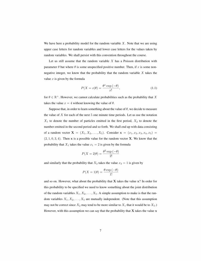
Let us plug in the observed x = 5, so that we get a function of θ that is called
likelihood function
l(θ) =θ5e−θ
120.
The graph of it is presented on the next figure. Can you localize on this graph the values
of probabilities that were used to chose θ = 7 over θ = 2? What value of θ appears to
be the most preferable if the same argument is extended to all possible values of θ? We
observe that the value of θ = 5 is most likely to produce value x = 5. In the result of
our likelihood approach we have used the data x = 5 and the Poisson model to make
inference - an example of statistical inference .
10
0 5 10 15
0.00
0.05
0.10
0.15
theta
Likelihood
Figure 1.4: Likelihood function for the Poisson model when the observed value is
x = 5.
Likelihood – Poisson model backward
Poisson model can be stated as a probability mass function that maps possible values
x into probabilities p(x) or if we emphasize the dependence on θ into p(x|θ) that is
given below
p(x|θ) = l(θ|x) =θxe−θ
x!,
• With the Poisson model with given θ one can compute probabilities that various
possible numbers x of emitted particles can be recorded, i.e. we consider
x 7→ p(x|θ)
with θ fixed. We get the answer how probable are various outcomes x.
• With the Poisson model where x is observed and thus fixed one can evaluate how
likely it would be to get x under various values of θ, i.e. we consider
θ 7→ l(θ|x)
with θ fixed. We get the answer how likely various θ could produced the observed
x.
11

Exercise 1. For the general Poisson model
p(x|θ) = l(θ|x) =θxe−θ
x!,
1. for a given θ > find the most probable value of the observation x.
2. for a given observation x find the most likely value of θ.
Give a mathematical argument for your claims.
1.2.2 More data
Suppose that we perform another measurement of the number of emitted particles. Let
us use the notation X1 to denote the number of particles emitted in the first period, X2
to denote the number emitted in the second period. We shall end up with data consisting
of a random vector X = (X1, X2). The second measurement yielded x2 = 2, so that
x = (x1, x2) = (5, 2).
We know that the probability thatX1 takes the value x1 = 5 is given by the formula
P (X = 5|θ) =θ5e−θ
5!
and similarly that the probability that X2 takes the value x2 = 2 is given by
P (X = 2|θ) =θ2e−θ
2!.
However, what about the probability that X takes the value x = (5, 2)? In order for
this probability to be specified we need to know something about the joint distribution
of the random variables X1, X2. A simple assumption to make is that the random
variables X1, X2 are mutually independent. In such a case the probability that X takes
the value x = (x1, x2) is given by
P (X = (x1, x2)|θ) =θx1e−θ
x1!· θ
x2e−θ
x2!= e−2θ θ
x1+x2
x1!x2!.
After little of algebra we easily find the likelihood function of observing X = (5, 2)
as
l(θ|(5, 2)) = e−2θ θ7
240
12

0 5 10 15
0.000
0.005
0.010
0.015
0.020
0.025
theta
Likelihood
0 5 10 15
0.00
0.05
0.10
0.15
theta
Likelihood
Figure 1.5: Likelihood of observing (5, 2) (top) vs. the one of observing 5 (bottom).
and its graph is presented in Figure 1.5 in comparison with the previous likelihood for
a single observation.
Two important effects of adding an extra information should be noted
• We observe that the location of the maximum shifted from 5 to 3 compared to
single observation.
• We also note that the range of likely values for θ has diminished.
Let us suppose that eventually we decide to measure three more values of X .
Let us use the vector notation X = (X1, X2, . . . , X5) to denote observable random
13

vector. Assume that three extra measurements yielded 3, 7, 7 so that we have x =
(x1, x2, x3, x4, x5) = (5, 2, 3, 7, 7). Under the assumption of independence the proba-
bility that X takes the value x is given by
P (X = x|θ) =5∏i=1
θxie−θ
xi!.
The likelihood function of observing X = (5, 2, 3, 7, 7) under independence can
be easily derived to beθ24e−5θ
14515200.
In general, if X = (x1, . . . , xn) is any vector of 5 non-negative integers, then the
likelihood is given by
l(θ|(x1, . . . , xn) =θ∑ni=1 xie−nθ
n∏i=1
xi!.
The value θ that maximizes this likelihood is called the maximum likelihood estimator
of θ.
In order to find values that effectively maximize likelihood, the method of calculus
can be implemented. We note that in our example we deal only with one variable θ and
computation of derivative is rather straightforward.
Exercise 2. For the general case of likelihood based on Poisson model
l(θ|x1, . . . , xn) =θ∑ni=1 xie−nθ
n∏i=1
xi!
using methods of calculus derive a general formula for the maximum likelihood esti-
mator of θ. Using the result find θ for (x1, x2, x3, x4, x5) = (5, 2, 3, 7, 7).
Exercise 3. It is generally believed that time X that passes until there is half of the
original radioactive material follow exponential distribution f(x|θ) = θe−θx, x > 0.
For beryllium 11 five experiments has been performed and values 13.21, 13.12, 13.95,
13.54, 13.88 seconds has been obtained. Find and plot the likelihood function for θ and
based on this determine the most likely θ.
14

1.3 Likelihood and theory of statistics
The strategy of making statistical inference based on the likelihood function as de-
scribed above is the recurrent theme in mathematical statistics and thus in our lecture.
Using mathematical argument we would compare various strategies to infering about
the parameters and often we will demonstrate that the likelihood based methods are
optimal. It will show its strength also as a criterium deciding between various claims
about parameters of the model which is the leading story of testing hypotheses.
In the modern days, the role of computers has increased in statistical methodology.
New computationally intense methods of data explorations become one of the central
areas of modern statistcs. Even there, methods that refer to likelihood play dominant
roles, in particular, in Bayesian methodology.
Despite this extensive penetration of statistical methodology by likelihood techin-
ques, by no means statistics can be reduced to analysis of likelihood. In every area of
statistics, there are important aspects that require reaching beyond likelihood, in many
cases, likelihood is not even a focus of studies and development. The purpose of this
course is to present both the importance of likelihood approach across statistics but also
presentation of topics for which likelihood plays a secondary role if any.
1.4 Computationally intensive methods of statistics
The second part of our presentation of modern statistical inference is devoted to compu-
tationally intensive statistical methods. The area of data explorations is rapidly growing
in importance due to
• common access to inexpensive but advance computing tools,
• emerging of new challenges associated with massive highly dimensional data far
exceeding traditional assumptions on which traditional methods of statistics have
been based.
In this introduction we give two examples that illustrate the power of modern computers
and computing software both in analysis of statistical models and in performing actual
15

statistical inference. We start with analyzing a performance of a statistical procedure
using random sample generation.
1.4.1 Monte Carlo methods – studying statistical methods using
computer generated random samples
Randomness can be used to study properties of a mathematical model. The model itself
may be probabilistic or not but here we focus on the probabilistic ones. Essentially, it
is based on repetitive simulations of random samples corresponding to the model and
observing behavior of objects of interests. An example of Monte Carlo method is ap-
proximate the area of circle by tossing randomly a point (typically computer generated)
on the paper where a circle is drawn. The percentage of points that fall inside the circle
represents (approximately) percentage of the area covered by the circle, as illustrated
in Figure 1.6.
Exercise 4. Write an R code that would explore the area of an elipsoid using Monte
Carlo method.
Below we present an application of Monte Carlo approach to studying fitting meth-
ods for the Poisson model.
Deciding for Poisson model
Recall that the Poisson model is given by
P (X = x|θ) =θxe−θ
x!.
It is relatively easy to demonstrate that the mean value of this distribution is equal to θ
and standard deviation is also equal to θ.
Exercise 5. Present a formal argument showing that for a Poisson random variable X
with parameter θ, EX = θ and VarX = θ.
Thus for a sample of observations x = (x1, . . . , xn) it is reasonable to consider
16

Figure 1.6: Monte Carlo study of the circle area – approximation for sample size of
10000 is 3.1248 which compares to the true value of π = 3.141593.
both
θ1 = x,
θ2 = x2 − x2
as estimators of θ.
We want to employ Monte Carlo method to decide which one is better. In the
process we run many samples from the Poisson distribution and check which of the
17

Histogram of means
means
Frequency
2.5 3.0 3.5 4.0 4.5 5.0 5.5
0100
Histogram of vars
vars
Frequency
0 5 10 15
0150
300
Figure 1.7: Monte Carlo results of comparing estimation of θ = 4 by the sample mean
(left) vs. estimation using the sample standard deviation right.
estimates performs better. The resulting histograms of the values of estimator are pre-
sented in Figure 1.8. It is quite clear from the graphs that the estimator based on the
mean is better than the one based on the variance.
1.4.2 Bootstrap – performing statistical inference using computers
Bootstrap (resampling) methods are one of the examples of Monte Carlo based statis-
tical analysis. The methodology can be summarized as follows
• Collect statistical sample, i.e. the same type of data as in classical statistics.
• Used a properly chosen Monte Carlo based resampling from the data using RNG
– create so called bootstrap samples.
• Analyze bootstrap samples to draw conclusions about the random mechanism
18

that produced the original statistical data.
This way randomness is used to analyze statistical samples that, by the way, are also a
result of randomness. An example illustrating the approach is presented next.
Estimating nitrate ion concentration
Nitrate ion concentration measurements in a certain chemical lab has been collected
and their results are given in the following table. The goal is to estimate, based on
0.51 0.51 0.51 0.50 0.51 0.49 0.52 0.53 0.50 0.47
0.51 0.52 0.53 0.48 0.49 0.50 0.52 0.49 0.49 0.50
0.49 0.48 0.46 0.49 0.49 0.48 0.49 0.49 0.51 0.47
0.51 0.51 0.51 0.48 0.50 0.47 0.50 0.51 0.49 0.48
0.51 0.50 0.50 0.53 0.52 0.52 0.50 0.50 0.51 0.51
Table 1.1: Results of 50 determinations of nitrate ion concentration in µg per ml.
these values, the actual nitrate ion concentration. The overall mean of all observations
is 0.4998. It is natural to ask what is the error of this determination of the nitrate
concentration. If we would repeat our experiment of collecting 50 samples of nitrate
concentrations many times we would see the range of error that is made. However,
it would be a waste of resources and not a viable method at all. Instead we resample
‘new’ data from our data and use so obtained new samples for assessment of the error
and compare the obtained means (bootstrap means) with the original one. The differ-
ences of these represent the bootstrap “estimation” errors their distribution is viewed
as a good representation of the distribution of the true error. In Figure ??, we see the
bootstrap counterpart of the distribution of the estimation error.
Based on this we can safely say that the nitrate concentration is 49.99± 0.005.
Exercise 6. Consider a sample of daily number of buyers in a furniture store
8, 5, 2, 3, 1, 3, 9, 5, 5, 2, 3, 3, 8, 4, 7, 11, 7, 5, 12, 5
Consider the two estimators of θ for a Poisson distribution as discussed in the previous
section. Describe formally the procedure (in steps) of obtaining a bootstrap confidence
19

Histogram of bootstrap
bootstrap
Frequency
-0.006 -0.004 -0.002 0.000 0.002 0.004 0.006 0.008
020
4060
80
Figure 1.8: Boostrap estimation error distribution.
interval for θ using each of the discussed estimatoand provide with 95% bootstrap
confidence intervals for each of them.
20

Chapter 2
Review of Probability
2.1 Expectation and Variance
The expected value E[Y ] of a random variable Y is defined as
E[Y ] =∞∑i=0
yiP (yi);
if Y is discrete, and
E[Y ] =∫ ∞−∞
yf(y)dy;
if Y is continuous, where f(y) is the probability density function. The variance Var[Y ]
of a random variable Y is defined as
Var[Y ] = E(Y − E[Y ])2;
or
Var[Y ] =∞∑i=0
(yi − E[Y ])2P (yi);
if Y is discrete, and
V ar[Y ] =∫ ∞−∞
(y − E[Y ])2f(y)dy;
if Y is continuous. When there is no ambiguity we often write EY for E[Y ], and VarY
for Var[Y ].
21

A function of a random variable is itself a random variable. If h(Y ) is function of
the random variable Y , then the expected value of h(Y ) is given by
E[h(Y )] =∞∑i=0
h(yi)P (yi);
if Y is discrete, and if Y is continuous
E[h(Y )] =∫ ∞−∞
h(y)f(y) dy.
It is relatively straightforward to derive the following results for the expectation
and variance of a linear function of Y .
E[aY + b] = aE[Y ] + b,
V ar[aY + b] = a2Var[Y ],
where a and b are constants. Also
Var[Y ] = E[Y 2]− (E[Y ])2 (2.1)
For expectations, it can be shown more generally that
Ek∑i=1
aihi(Y ) =k∑i=1
aiE[hi(Y )],
where ai, i = 1, 2, . . . , k are constants and hi(Y ), i = 1, 2, . . . , k are functions of the
random variable Y .
2.2 Distribution of a Function of a Random Variable
If Y is a random variable than for any regular function X = g(Y ) is also a random
variable. The cumulative distribution function of X is given as
FX(x) = P (X ≤ x) = P (Y ∈ g−1(−∞, x]).
The density function of X if exists can be found by differentiating the right hand side
of the above equality.
22

Example 1. Let Y has a density fY and X = Y 2. Then
FX(x) = P (Y 2 < x) = P (−√x ≤ Y ≤
√x) = FY (
√x)− FY (−
√x).
By taking a derivative in x we obtain
fX(x) =1
2√x
(fY (√x) + fY (−
√x)).
If additionally the distribution of Y is symmetric around zero, i.e. fY (y) = fY (−y),
then
fX(x) =1√xfY (√x).
Exercise 7. Let Z be a random variable with the density fZ(z) = e−z2/2/√
2π, so
called the standard normal (Gaussian) random variable. Show thatZ2 is aGamma(1/2, 1/2)
random variable, i.e. that it has the density given by
1√2πx−1/2e−x/2.
The distribution ofZ2 is also called chi-square distribution with one degree of freedom.
Exercise 8. Let FY (y) be a cumulative distribution function of some random variable
Y that with probability one takes values in a set RY . Assume that there is an inverse
function F−1Y [0, 1] 7→ RY so that FY F−1
Y (u) = u for u ∈ [0, 1]. Check that for U ∼
Unif(0, 1) the random variable Y = F−1Y (U) has FY as its cumulative distribution
function.
The densities of g(Y ) are particularly easy to express if g is a strictly monotone as
shown in the next result
Theorem 2.2.1. Let Y be a continuous random variable with probability density func-
tion fY . Suppose that g(y) is a strictly monotone (increasing or decreasing) differ-
entiable (and hence continuous) function of y. The random variable Z defined by
Z = g(Y ) has probability density function given by
fZ(z) = fY(g−1(z)
) ∣∣∣∣ ddz g−a(z)∣∣∣∣ (2.2)
where g−1(z) is defined to be the inverse function of g(y).
23

Proof. Let g(y) be a monotone increasing (decreasing) function and let FY (y) and
FZ(z) denote the probability distribution functions of the random variables Y and Z.
Then
FZ(z) = P (Z ≤ z) = P (g(Y ) ≤ z) = P (Y ≤ (≥)g−1(z)) = (1−)FY (g−1(z))
By the chain rule,
fZ(z) =d
dzFZ(z) = (−)
d
dzFY (g−1(z)) = fY (g−1(z))
∣∣∣∣dg−1
dz(z)∣∣∣∣ .
Exercise 9. (The Log-Normal Distribution) Suppose Z is a standard normal distribu-
tion and g(z) = eaz+b. Then Y = g(Z) is called a log-normal random variable.
Demonstrate that the density of Y is given by
fY (y) =1√
2πa2y−1 exp
(− log2(y/eb)
2a2
).
2.3 Transforms Method Characteristic, Probability Gen-
erating and Moment Generating Functions
The probability generating function of a random variable Y is a function denoted by
GY (t) and defined by
GY (t) = E(tY ),
for those t ∈ R for which the above expectation is convergent. The expectation defining
GY (t) converges absolutely if |t| ≤ 1. As the name implies, the p.g.f generates the
probabilities associated with a discrete distribution P (Y = j) = pj , j = 0, 1, 2, . . . .
GY (0) = p0, G′Y (0) = p1, G”Y (0) = 2!p2.
In general the kth derivative of the p.g.f of Y satisfies
G(k)Y (0) = k!pk.
24

The p.g.f can be used to calculate the mean and variance of a random variable Y . Note
that in the discrete case G′Y (t) =∑∞j=1 jpjt
j−1 for −1 < t < 1. Let t approach one
from the left, t→ 1−, to obtain
G′Y (1) =∞∑j=1
jpj = E(Y ) = µY .
The second derivative of GY (t) satisfies
G”Y (t) =∞∑j=1
j(j − 1)pjtj−2,
and consequently
G”Y (1) =∞∑j = 1j(j − 1)pj = E(Y 2)− E2(Y ).
The variance of Y satisfies
σ2Y = EY 2 − EY + EY − E2Y = G”Y (1) +G′Y (1)−G′2Y (1).
The moment generating function (m.g.f) of a random variable Y is denoted by
MY (t) and defined as
MY (t) = E(etY),
for some t ∈ R. The moment generating function generates the moments EY k
MY (0) = 1, M ′Y (0) = µY = E(Y ), M”Y (0) = EY 2,
and, in general,
M (k)Y (0) = EY k.
The characteristic function (ch.f) of a random variable Y is defined by
φY (t) = EeitY ,
where i =√−1.
A very important result concerning generating functions states that the moment
generating function uniquely defines the probability distribution (provided it exists in
an open interval around zero). The characteristic function also uniquely defines the
probability distribution.
25

Property 1. If Y has the characteristic function φY (t) and the moment generating
function MY (t), then for X = a+ bY
φX(t) =eaitφY (bt)
MX(t) =eatMY (bt).
2.4 Random Vectors
2.4.1 Sums of Independent Random Variables
Suppose that Y1, Y2, . . . , Yn are independent random variables. Then the moment gen-
erating function of the linear combination Z =∑ni=1 aiYi is the product of the indi-
vidual moment generating functions.
MZ(t) =Eet∑aiYi
=Eea1tY1Eea2tY2 · · ·EeantYn
=n∏i=1
MYi(aiYi).
The same argument gives also that φZ(t) =∏ni=1 φYi(aiY i).
When X and Y are discrete random variables, the condition of independence is
equiva- lent to pX,Y (x, y) = pX(x)pY (y) for all x, y. In the jointly continuous case
the condition of independence is equivalent to fX,Y (x, y) = fX(x)fY (y) for all x, y.
Consider random variables X and Y with probability densities fX(x) and fY (y) re-
spectively. We seek the probability density of the random variable X+Y . Our general
result follows from
FX+Y (a) =P (X + Y < a)
=∫ ∫
X+Y <a
fX(x)fY (y) dxdy
=∫ ∞−∞
∫ a−y
−∞fX(x)fY (y) dxdy
=∫ ∞−∞
∫ a
−∞fX(z − y) dz fY (y) dy
=∫ a
−∞
∫ ∞−∞
fX(z − y)fY (y) dy dz
(2.3)
26

Thus the density function fX+Y (z) =∫∞−∞ fX(z − y)fY (y) dy which is called the
convolution of the densities fX and fY .
2.4.2 Covariance and Correlation
Suppose that X and Y are real-valued random variables for some random experiment.
The covariance of X and Y is defined by
Cov(X,Y ) = E[(X − EX)(Y − EY )]
and (assuming the variances are positive) the correlation of X and Y is defined by
ρ(X,Y ) =Cov(X,Y )√
Var(X)√
Var(Y ).
Note that the covariance and correlation always have the same sign (positive, nega-
tive, or 0). When the sign is positive, the variables are said to be positively correlated,
when the sign is negative, the variables are said to be negatively correlated, and when
the sign is 0, the variables are said to be uncorrelated. For an intuitive understanding
of correlation, suppose that we run the experiment a large number of times and that
for each run, we plot the values (X,Y ) in a scatterplot. The scatterplot for positively
correlated variables shows a linear trend with positive slope, while the scatterplot for
negatively correlated variables shows a linear trend with negative slope. For uncorre-
lated variables, the scatterplot should look like an amorphous blob of points with no
discernible linear trend.
Property 2. You should satisfy yourself that the following are true
Cov(X,Y ) =EXY − EXEY
Cov(X,Y ) =Cov(Y,X)
Cov(Y, Y ) =Var(Y )
Cov(aX + bY + c, Z) =aCov(X,Z) + bCov(Y, Z)
Var
(n∑i=1
Yi
)=
n∑i,j=1
Cov(Yi, Yj)
If X and Y are independent, then they are uncorrelated. The converse is not true
however.
27

2.4.3 The Bivariate Change of Variables Formula
Suppose that (X,Y ) is a random vector taking values in a subset S of R2 with proba-
bility density function f . Suppose that U and V are random variables that are functions
of X and Y
U = U(X,Y ), V = V (X,Y ).
If these functions have derivatives, there is a simple way to get the joint probability
density function g of (U, V ). First, we will assume that the transformation (x, y) 7→
(u, v) is one-to-one and maps S onto a subset T of R2. Thus, the inverse transformation
(u, v) 7→ (x, y) is well defined and maps T onto S. We will assume that the inverse
transformation is “smooth”, in the sense that the partial derivatives
∂x
∂u,∂x
∂v,∂y
∂u,∂y
∂v,
exist on T , and the Jacobian
∂(x, y)∂(u, v)
=
∣∣∣∣∣∣∂x∂u
∂x∂v
∂y∂u
∂y∂v
∣∣∣∣∣∣ =∂x
∂u
∂y
∂v− ∂x
∂v
∂y
∂u
is nonzero on T . Now, let B be an arbitrary subset of T . The inverse transformation
maps B onto a subset A of S. Therefore,
P ((U, V ) ∈ B) = P ((X,Y ) ∈ A) =∫ ∫
A
f(x, y) dxdy.
But, by the change of variables formula for double integrals, this can be written as
P ((U, V ) ∈ B) =∫ ∫
B
f(x(u, v), y(u, y))∣∣∣∣∂(x, y)∂(u, v)
∣∣∣∣ dudv.By the very meaning of density, it follows that the probability density function of
(U, V ) is
g(u, v) = f(x(u, v), y(u, v))∣∣∣∣∂(x, y)∂(u, v)
∣∣∣∣ , (u, v) ∈ T.
The change of variables formula generalizes to Rn.
Exercise 10. Let U1 and U2 be independent random variables with the density equal
to one over [0, 1], i.e. standard uniform random variables. Find the density of the
following vector of variables
(Z1, Z2) = (√−2 logU1 cos(2πU2),
√−2 logU1 sin(2πU2)).
28

2.5 Discrete Random Variables
2.5.1 Bernoulli Distribution
A Bernoulli trial is a probabilistic experiment which can have one of two outcomes,
success (Y = 1) or failure (Y = 0) and in which the probability of success is θ. We
refer to θ as the Bernoulli probability parameter. The value of the random variable Y is
used as an indicator of the outcome, which may also be interpreted as the presence or
absence of a particular characteristic. A Bernoulli random variable Y has probability
mass function
P (Y = y|θ) = θy(1− θ)1 − y (2.4)
for y = 0, 1 and some θ ∈ (0, 1). The notation Y ∼ Ber(θ) should be read as the
random variable Y follows a Bernoulli distribution with parameter θ.
A Bernoulli random variable Y has expected value E[Y ] = 0 · P (Y = 0) + 1 ·
P (Y = 1) = 0·(1−θ)+1·θ = θ, and variance Var[Y ] = (0−θ)2·(1−θ)+(1−θ)2·θ =
θ(1− θ).
2.5.2 Binomial Distribution
Consider independent repetitions of Bernoulli experiments, each with a probability of
success θ. Next consider the random variable Y , defined as the number of successes in
a fixed number of independent Bernoulli trials, n . That is,
Y =n∑i=1
Xi,
where Xi ∼ Bernoulli(θ) for i = 1, . . . , n. Each sequence of length n containing y
“ones” and (n− y) “zeros” occurs with probability θy(1− θ)(n− y). The number of
sequences with y successes, and consequently (n− y) fails, is
n!y!(n− y)!
=(n
y
).
The random variable Y can take on values y = 0, 1, 2, . . . , n with probabilities
P (Y = y|θ) =(n
y
)θy(1− θ)n−y. (2.5)
29
The notation Y ∼ Bin(n, θ) should be read as “the random variable Y follows a bi-
nomial distribution with parameters n and θ.” Finally using the fact that Y is the sum
of n independent Bernoulli random variables we can calculate the expected value as
E[Y ] = E[∑Xi] = PE[Xi] =
∑θ = nθ and variance as Var[Y ] = V ar[
∑Xi] =∑
Var[Xi] =∑θ(1− θ) = nθ(1− θ).
2.5.3 Negative Binomial and Geometric Distribution
Instead of fixing the number of trials, suppose now that the number of successes, r,
is fixed, and that the sample size required in order to reach this fixed number is the
random variable N . This is sometimes called inverse sampling. In the case of r = 1,
using the independence argument again, leads to geomoetric distribution
P (N = n|θ) = θ(1− θ)n−1, n = 1, 2, . . . (2.6)
for n = 1, 2, . . . which is the geometric probability function with parameter θ. The
distribution is so named as successive probabilities form a geometric series. The no-
tation N ∼ Geo(θ) should be read as “the random variable N follows a geometric
distribution with parameter θ.” Write (1− θ) = q. Then
E[N ] =∞∑n=1
nqnθ = θ
∞∑n=0
d
dq(qn) = θ
d
dq
( ∞∑n=0
qn
)
= θd
dq
(1
1− q
)=
θ
(1− q)2=
1θ.
Also,
E[N2] =∞∑n=1
n2qn−1θ = θ
∞∑n=1
d
dq(nqn) = θ
d
dq
( ∞∑n=1
nqn
)
= θd
dqθ
(q
1− qE(N)
)= θ
d
dq
(q(1− q)−2
)= θ
(1θ2
+2(1− θ)θ3
)=
2θ2− 1θ.
Using Var[N ] = E[N2]− (E[N ])2, we get Var[N ] = (1− θ)/θ2.
Consider now sampling continues until a total of r successes are observed. Again,
let the random variable N denote number of trial required. If the rth success occurs
30

on the nth trial, then this implies that a total of (r − 1) successes are observed by the
(n− 1)th trial. The probability of this happening can be calculated using the binomial
distribution as (n− 1r − 1
)θr−1(1− θ)n−r.
The probability that the nth trial is a success is θ. As these two events are indepen-
dent we have that
P (N = n|r, θ) =(n− 1r − 1
)θr(1− θ)n−r (2.7)
for n = r, r + 1, . . . . The notation N ∼ NegBin(r, θ) should be read as “the random
variable N follows a negative binomial distribution with parameters r and θ.” This is
also known as the Pascal distribution.
E[Nk] =∞∑n=r
nk(n− 1r − 1
)θr(1− θ)n−r
=r
θ
∞∑n=r
nk−1
(n
r
)θr+1(1− θ)n−r since n
(n− 1r − 1
)= r
(n
r
)
=r
θ
∞∑m=r+1
(m− 1)k−1
(m− 1r
)θr+1(1− θ)m−(r+1)
=r
θE[(X − 1)k−1
],
where X ∼ Negativebinomial(r+ 1, θ). Setting k = 1 we get E(N) = r/θ. Setting
k = 2 gives
E[N2] =r
θE(X − 1) =
r
θ
(r + 1θ− 1).
Therefore Var[N ] = r(1− θ)/θ2.
2.5.4 Hypergeometric Distribution
The hypergeometric distribution is used to describe sampling without replacement.
Consider an urn containing b balls, of which w are white and b − w are red. We
intend to draw a sample of size n from the urn. Let Y denote the number of white balls
selected. Then, for y = 0, 1, 2, . . . , n we have
P (Y = y|b, w, n) =
(wy
)(b−wn−y)(
bn
) . (2.8)
31

The expected value of the jth moment of a hypergeometric random variable is
E[Y ] =n∑y=0
yjP (Y = y) =n∑y=1
yj
(wy
)(b−wn−y)(
bn
) .
The identities
y
(w
y
)= w
(w − 1y − 1
)n
(b
n
)= b
(b− 1n− 1
)can be used to obtain
E[Y j ] =nw
b
n∑y=1
yj−1
(w−1y−1
)(b−wn−1
)(b−1n−1
)=nw
b
n−1∑x=0
(x+ 1)j−1
(w−1x
)(b−wn−1−x
)(b−1n−1
)=nw
bE[(X + 1)j−1]
whereX is a hypergeometric random variable with parameters n−1, b−1,w−1. From
this it is easy to establish that E[Y ] = nθ and Var[Y ] = nθ(1 − θ)(b − n)/(b − 1),
where θ = w/b is the fraction of white balls in the population.
2.5.5 Poisson Distribution
Certain problems involve counting the number of events that have occurred in a fixed
time period. A random variable Y , taking on one of the values 0, 1, 2, . . . , is said to be
a Poisson random variable with parameter θ if for some θ > 0,
P (Y = y|θ) =θy
y!e−θ, y = 0, 1, 2, . . . (2.9)
The notation Y ∼ Pois(θ) should be read as “random variable Y follows a Poisson
distribution with parameter θ.” Equation 2.9 defines a probability mass function, since∞∑y=0
θy
y!e−θ = e−θ
∞∑y=0
θy
y!= e−θeθ = 1.
The expected value of a Poisson random variable is
E[Y ] =∞∑y=0
ye−θθy
y!= θe−θ
∞∑y=1
θy−1
(y − 1)!= θe−θ
∞∑j=0
θj
(j)!= θ.
32

To get the variance we first compute the second moment
E[Y 2] =∞∑y=0
y2e−θθy
y!= θ
∞∑y=1
ye−θθy−1
y − 1!= θ
∞∑j=0
(j + 1)e−θθj
j!= θ(θ + 1).
Since we already have E[Y ] = θ, we obtain Var[Y ] = E[Y 2]− (E[Y ])2 = θ.
Suppose that Y ∼ Binomial(n, p), and let θ = np. Then
P (Y = y|np) =(n
y
)py(1− p)n−y
=(n
y
)(θ
n
)y (1− θ
n
)n−y=n(n− 1) · · · (n− y + 1)
nyθy
y!(1− θ/n)n
(1− θ/n)y.
For n large and θ “moderate”, we have that(1− θ
n
)n≈ e−θ, n(n− 1) · · · (n− y + 1)
ny≈ 1,
(1− θ
n
)y≈ 1.
Our result is that a binomial random variable Bin(n, p) is well approximated by a
Poisson random variable Pois(θ = np) when n is large and p is small. That is
P (Y = y|n, p) ≈ e−np (np)y
y!.
2.5.6 Discrete Uniform Distribution
The discrete uniform distribution with integer parameter N has a random variable Y
that can take the vales y = 1, 2, . . . , N with equal probability 1/N . It is easy to show
that the mean and variance of Y are E[Y ] = (N + 1)/2, and Var[Y ] = (N2 − 1)/12.
2.5.7 The Multinomial Distribution
Suppose that we perform n independent and identical experiments, where each ex-
periment can result in any one of r possible outcomes, with respective probabilities
p1, p2, . . . , pr, where∑ri=1 pi = 1. If we denote by Yi, the number of the n experi-
ments that result in outcome number i, then
P (Y1 = n1, Y2 = n2, . . . , Yr = nr) =n!
n1!n2! · · ·nr!pn1
1 pn22 · · · p
nr5 (2.10)
33

where∑ri=1 ni = n. Equation 2.10 is justified by noting that any sequence of out-
comes that leads to outcome i occurring ni times for i = 1, 2, . . . , r, will, by the
assumption of independence of experiments, have probability pn11 pn2
2 · · · pnrr of occur-
ring. As there are n! = (n1!n2! · · ·nr!) such sequence of outcomes equation 2.10 is
established.
2.6 Continuous Random Variables
2.6.1 Uniform Distribution
A random variable Y is said to be uniformly distributed over the interval (a, b) if its
probability density function is given by
f(y|a, b) =1
b− a, if a < y < b
and equals 0 for all other values of y. Since F (u) =∫ u−∞ f(y)dy, the distribution
function of a uniform random variable on the interval (a, b) is
F (u) =
0; u ≤ a,
(u− a)/(b− a); a < u ≤ b,
1; u > b
The expected value of a uniform random turns out to be the mid-point of the interval,
that is
E[Y ] =∫ ∞−∞
yf(y)dy =∫ b
a
y
b− ady =
b2 − a2
2(b− a)=b+ a
2.
The second moment is calculated as
E[Y 2] =∫ b
a
y2
b− ady =
b3 − a3
3(b− a)=
13
(b2 + ab+ a2),
hence the variance is
Var[Y ] = E[Y 2]− (E[Y ])2 =112
(b− a)2.
The notation Y ∼ U(a, b) should be read as “the random variable Y follows a uniform
distribution on the interval (a, b)”.
34

2.6.2 Exponential Distribution
A random variable Y is said to be an exponential random variable if its probability
density function is given by
f(y|θ) = θe−θy, y > 0, θ > 0.
The cumulative distribution of an exponential random variable is given by
F (a) =∫ a
0
θe−θydy = −e−θy|a0 = 1− e−θa, a > 0.
The expected value E[Y ] =∫∞
0yθe−θy dy requires integration by parts, yielding
E[Y ] = −ye−θy|∞0 +∫ ∞
0
e−θy dy =−e−θy
θ|∞0 =
1θ.
Integration by parts can be used to verify that E[Y 2] = 2θ−2. Hence Var[Y ] = 1/θ2.
The notation Y ∼ Exp(θ) should be read as “the random variable Y follows an expo-
nential distribution with parameter θ”.
Exercise 11. Let Y ∼ U [0, 1]. Find the distribution of Y = − logU . Can you identify
it as a one of the common distributions?
2.6.3 Gamma Distribution
A random variable Y is said to have a gamma distribution if its density function is
given by
f(y|αθ) = θαe−θyyα−1/Γ(α), 0 < y, λ > 0, θ > 0
where Γ(α), is called the gamma function and is defined by
Γ(α) =∫ ∞
0
e−uuα−1du.
The integration by parts of Γ(α) yields the recursive relationship
Γ(α) = −e−uuα−1|∞0 +∫ ∞
0
e−u(α− 1)uα−2 du (2.11)
= (α− 1)∫ ∞
0
e−uuα−2 du = (α− 1)Γ(α− 1). (2.12)
35

For integer values α = n, this recursive relationship reduces to Γ(n + 1) = n!. Note,
by setting α = 1 the gamma distribution reduces to an exponential distribution. The
expected value of a gamma random variable is given by
E[Y ] =θα
Γ(α)
∫ ∞0
yαe−θy dy = θ!θα
Γ(α)
∫ ∞0
uαe−u du,
after the change of variable u = θy. Hence E[Y ] = Γ(α+ 1)/(Γ(α)θ) = α/θ. Using
the same substitution
E[Y 2] =θα
Γ(α)
∫ ∞0
yω+1e−θy dy =(α+ 1)α
θ2,
so that Var[Y ] = α/θ2. The notation Y ∼ Gamma(α, θ) should be read as “the
random variable Y follows a gamma distribution with parameters α and θ”.
Exercise 12. Let Y ∼ Gamma(α, θ). Show that the moment generating function for
Y is given for t ∈ (−θ, θ) by
MY (t) =1
(1− t/θ)α.
2.6.4 Gaussian (Normal) Distribution
A random variable Z is a standard normal (or Gaussian) random variable if the density
of Z is specified by
f(z) =1√2πe−z
2/2. (2.13)
It is not immediately obvious that (2.13) specifies a probability density. To show that
this is the case we need to prove∫ ∞−∞
1√2πe−z
2/2dy = 1
or, equivalently, that I =∫∞−∞ e−z
2/2 dz =√
2π. This is a “classic” results and so is
well worth confirming. Consider
I2 =∫ ∞−∞
e− z2/2 dz∫ ∞−∞
e−w2/2 dw =∫ ∞−∞
∫ ∞−∞
e−(z2+w2)/2 dzdw.
The double integral can be evaluated by a change of variables to polar coordinates.
Substituting z = r cos θ, w = r sin θ, and dzdw = rdθdr, we get
I2 =∫ ∞
0
∫ π
0
e−r2/2rdθdr = 2π
∫ ∞0
re−r2/2 dr = −2πe−r2/2|10 = 2π.
36

Taking the square root we get I =√
2π. The result I =√
2π can also be used to
establish the result Γ(1/2) =√π. To prove that this is the case note that
Γ(1/2) =∫ ∞
0
e−uu1/2 du = 2∫ ∞
0
e−z2dz =
√π.
The expected value of Z equals zero because ze−z2/2 is integrable and asymmetric
around zero. The variance of Z is given by
Var[Z] =1√2π
∫ ∞−∞
z2e−z2/2 dz.
Thus
Var[Z] =1√2π
∫ ∞−∞
z2e−z2/2 dz
=1√2π
[−ze−z
2/2|∞−∞ + +∫ ∞−∞
e− z2/2 dz]
=1√2π
∫ ∞−∞
e−z2/2 dz
=1.
If Z is a standard normal distribution then Y = µ + σZ is called general normal
(Gaussian distribution) with parameters µ and σ. The density of Y is given by
f(y|µ, σ) =1√
2πσ2e−
(y−µ)2
2σ2 .
We have obviously E[Y ] = µ and Var[Y ] = σ2. The notation Y ∼ N(µ, σ2) should
be read as “the random variable Y follows a normal distribution with mean parameter
µ and variance parameter σ2”. From the definition of Y it follows immediately that
a+ bY , where a and b are known constants, is again normal distribution.
Exercise 13. Let Y ∼ N(µ, σ2). What is the distribution of X = a+ bY ?
Exercise 14. Let Y ∼ N(µ, σ2). Show that the moment generating function if Y is
given by
MY (t) = eµt+σ2t2/2.
Hint Consider first the standard normal variable and then apply Property 1.
37

2.6.5 Weibull Distribution
The Weibull distribution function has the form
F (y) = 1− exp[−(yb
)a], y > 0.
The Weibull density can be obtained by differentiation as
f(y|a, b) =(ab
)(yb
)a−1
exp[−(yb
)a].
To calculate the expected value
E[Y ] =∫ ∞
0
ya
(1b
)aya−1 exp
[−(yb
)a]dy
we use the substitutions u = (y/b)a, and du = ab−aya−1dy. These yield
E[Y ] = b
∫ ∞0
u1/ae−udu = bΓ(a+ 1a
).
In a similar manner, it is straightforward to verify that
E[Y 2] = b2Γ(a+ 2a
),
and thus
Var[Y ] = b2(
Γ(a+ 2a
)− Γ2
(a+ 1a
)).
2.6.6 Beta Distribution
A random variable is said to have a beta distribution if its density is given by
f(y|a, b) =1
B(a, b)ya−1(1− y)b−1, 0 < y < 1.
Here the function
B(a, b) =∫ 1
0
ua−1(1− u)b−1 du
is the “beta” function, and is related to the gamma function through
B(a, b) =Γ(a)Γ(b)Γ(a+ b)
.
Proceeding in the usual manner, we can show that
E[Y ] =a
a+ b
Var[Y ] =ab
(a+ b)2(a+ b+ 1).
38

2.6.7 Chi-square Distribution
Let Z ∼ N(0, 1), and let Y = Z2. Then the cumulative distribution function
FY (y) = P (Y ≤ y) = P (Z2 ≤ y) = P (−√y ≤ Z ≤ √y) = FZ(√y)− FZ(−√y)
so that by differentiating in y we arrive to the density
fY (y) =1
2√y
[fz(√y) + fz(−
√y)] =
1√2πy
e−y/2,
in which we recognize Gamma(1/2, 1/2). Suppose that Y =∑ni=1 Z
2i , where the
Zi ∼ N(0, 1) for i = 1, . . . , n are independent. From results on the sum of indepen-
dent Gamma random variables, Y ∼ Gamma(n/2, 1/2). This density has the form
fY (y|n) =e−y/2yn/2−1
2n/2Γ(n/2), y > 0 (2.14)
and is referred to as a chi-squared distribution on n degrees of freedom. The notation
Y ∼ Chi(n) should be read as “the random variable Y follows a chi-squared dis-
tribution with n degrees of freedom”. Later we will show that if X ∼ Chi(u) and
Y ∼ Chi(v), it follows that X + Y ∼ Chi(u+ v).
2.6.8 The Bivariate Normal Distribution
Suppose thatU and V are independent random variables each, with the standard normal
distribution. We will need the following parameters µX , µY , σX > 0, σY > 0,
ρ ∈ [−1, 1]. Now let X and Y be new random variables defined by
X =µX + σXU,
V =µY + ρσY U + σY√
1− ρ2V.
Using basic properties of mean, variance, covariance, and the normal distribution, sat-
isfy yourself of the following.
Property 3. The following properties hold
1. X is normally distributed with mean µX and standard deviation σX ,
2. Y is normally distributed with mean µY and standard deviation σY ,
39

3. Corr(X,Y ) = ρ,
4. X and Y are independent if and only if ρ = 0.
The inverse transformation is
u =x− µXσX
v =y − µY
σY√
1− ρ2− ρ(x− µX)
σX√
1− ρ2
so that the Jacobian of the transformation is
∂(x, y)∂(u, v)
=1
σXσY√
1− ρ2.
Since U and V are independent standard normal variables, their joint probability den-
sity function is
g(u, v) =1
2πe−
u2+v22 .
Using the bivariate change of variables formula, the joint density of (X,Y ) is
f(x, y) =1
2πσXσY√
1− ρ2exp
[− (x− µX)2
2σ2X(1− ρ2)
+ρ(x− µX)(y − µY )σXσY (1− ρ2)
(y − µY )2
2σ2Y (1− ρ2)
]
Bivariate Normal Conditional Distributions
In the last section we derived the joint probability density function f of the bivariate
normal random variables X and Y . The marginal densities are known. Then,
fY |X(y|x) =fY,X(y, x)fX(x)
=1√
2πσ2Y (1− ρ2)
exp(− (y − (µY + ρσY (x− µX)/σX))2
2σ2Y (1− ρ2)
).
Then the conditional distribution of Y given X = x is also Gaussian, with
E(Y |X = x) =µY + ρσYx− µXσX
Var(Y |X = x) = σ2Y (1− ρ2)
2.6.9 The Multivariate Normal Distribution
Let Σ denote the 2× 2 symmetric matrix σ2X σXσY ρ
σY σXρ σ2Y
40

Then
det|Σ| = σ2Xσ
2Y − (σXσY ρ)2 = σ2
Xσ2Y (1− ρ2)
and
Σ−1 =1
1− ρ2
1/σ2X −ρ/(σXσY )
−ρ/(σXσY ) 1/σ2Y
.Hence the bivariate normal distribution (X,Y ) can be written in matrix notation as
f(X,Y )(x, y) =1
2π√det|Σ|
exp
−12
x− µXy − µY
T Σ−1
x− µXy − µY
.
Let Y = (Y 1, . . . , Y p) be a random vector. Let E(Yi) = µi, i = 1, . . . , p, and define
the p-length vector µ = (µ1, . . . , µp). Define the p × p matrix Σ through its elements
Cov(Yi, Yj) for i, j = 1, . . . p. Then, the random vector Y has a p-dimensional multi-
variate Gaussian distribution if its density function is specified by
fY (y) =1
(2π)p/2|Σ|1/2exp
(−1
2(y − µ)TΣ−1(y − µ)
). (2.15)
The notation Y ∼ MVNp(µ,Σ) should be read as “the random variable Y follows a
multivariate Gaussian (normal) distribution with p-vector mean µ and p × p variance-
covariance matrix Σ.”
41

2.7 Distributions – further properties
2.7.1 Sum of Independent Random Variables – special cases
Poisson variables
Suppose X ∼ Pois(θ) and Y ∼ Pois(λ). Assume that X and Y are independent.
Then
P (X + Y = n) =n∑k=0
P (X = k, Y = n− k)
=n∑k=0
P (X = k)P (Y = n− k)
=n∑k=0
e−θθk
k!e−λ
λn−k
(n− k)!
=e−(θ+λ)
n!
n∑k=0
n!k!(n− k)!
θkλn−k
=e− (θ + λ)(θ + λ)n
n!.
That is, X + Y ∼ Pois(θ + λ).
Binomial Random Variables
We seek the distribution of Y + X , where Y ∼ Bin(n, θ) and X ∼ Bin(m, θ).
Since X + Y is modelling the situation where the total number of trials is fixed at
n + m and the probability of a success in a single trial equals θ. Without performing
a calculations, we expect to find that X + Y ∼ Bin(n + m, θ). To verify that note
thatX = X1 + · · ·+Xn whereXi are independent Bernoulli variables with parameter
θ while Y = Y1 + · · · + Ym where Yi are also independent Bernoulli variables with
parameter θ. Assuming that Xi’s are independent of Yi’s we obtain that X + Y is the
sum of n + m indpendent Bernoulli random variables with parameter θ, i.e. X + Y
has Bin(n+m, θ) distribution.
42

Gamma, Chi-square, and Exponential Random Variables
Let X ∼ Gamma(α, θ) and Y ∼ Gamma(βθ) are independent. Then the moment
generating function of X + Y is given as
MX+Y (t) = MX(t)MY (t) =1
(1 + t/θ)α1
(1 + t/θ)β=
1(1 + t/θ)α+β
But this is the moment generating function of a Gamma random variable distributed
as Gamma(α + β, θ). The result X + Y ∼ Chi(u + v) where X ∼ Chi(u) and
Y ∼ Chi(v), follows as a corollary.
Let Y1, . . . , Yn be n independent exponential random variables each with parameter
θ. Then Z = Y1 + Y2 + · · · + Yn is a Gamma(n, θ) random variable. To see that
this is indeed the case, write Yi ∼ Exp(θ), or alternatively, Yi ∼ Gamma(1, θ). Then
Y1 + Y2 ∼ Gamma(2, θ), and by induction∑ni=1 Yi ∼ Gamma(n, θ).
Gaussian Random Variables
Let X ∼ N(µX , σ2X) and Y ∼ N(µY , σ2
Y ). Then the moment generating function of
X + Y is given by
MX+Y (t) = MX(t)MY (t) = eµXt+σ2Xt
2/2eµY t+σ2Y t
2/2 = e(µX+µY )t+(σ2X+σ2
Y )t2/2
which proves that X + Y ∼ N(µX + µY , σ2X + σ2
Y ).
43

44

2.7.2 Common Distributions – Summarizing TablesDiscrete Distributions
Bernoulli(θ)
pmf P (Y = y|θ) = θy(1− θ)1−y, y = 0, 1, 0 ≤ θ ≤ 1
mean/variance E[Y ] = θ,Var[Y ] = θ(1− θ)
mgf MY (t) = θet + (1− θ)
Binomial(n, θ)
pmf P (Y = y|θ) =(ny
)θy(1− θ)n−y, y = 0, 1, . . . , n, 0 ≤ θ ≤ 1
mean/variance E[Y ] = nθ,Var[Y ] = nθ(1− θ)
mgf MY (t) = [θet + (1− θ)]n
Discrete uniform(N )
pmf P (Y = y|N) = 1/N, y = 1, 2, . . . , N
mean/variance E[Y ] = (N + 1)/2,Var[Y ] = (N + 1)(N − 1)/12
mgf MY (t) = 1Net 1−eNt
1−et
Geometric(θ)
pmf P (Y = y|N) = θ(1− θ)y−1, y = 1, . . . , 0 ≤ θ ≤ 1
mean/variance E[Y ] = 1/θ,Var[Y ] = (1− θ)/θ2
mgf MY (t) = θet/[1− (1− θ)et], t < − log(1− θ)
notes The random variable X = Y − 1 is NegBin(1, θ).
Hypergeometric(b, w, n)
pmf P (Y = y|b, w, n) =(wy
)(b−wn−y
)/(bn
), y = 0, 1, . . . , n,
b− (b− w) ≤ y ≤ b, b, w, n ≥ 0
mean/variance E[Y ] = nw/b,Var[Y ] = nw(b− w)(b− n)/(b2(b− 1))
Negative binomial(r, θ)
pmf P (Y = y|r, θ) =(r+y−1y
)θr(1− θ)y, y = 0, 1, . . . , n,
b− (b− w) ≤ y ∈ N, 0 < θ ≤ 1
mean/variance E[Y ] = r(1− θ)/θ,Var[Y ] = r(1− θ)/θ2
mgf MY (t) = θ/(1− (1− θ)et)r, t < − log(1− θ)
notes
An alternative form of the pmf, used in the derivation in our notes, isgiven by P (N = n|r, θ) =
(n−1r−1
)θr(1 − θ)n−r , n = r, r + 1, . . .
where the random variableN = Y + r. The negative binomial can alsobe derived as a mixture of Poisson random variables.
Poisson(θ)
pmf P (Y = y|θ) = θye−θ/y!, y = 0, 1, 2, . . . , 0 < θ
mean/variance E[Y ] = θ,Var[Y ] = θ,
mgf MY (t) = eθ(et−1)
45

Continuous Distributions
Uniform U(a, b)
pmf f(y|a, b) = 1/(b− a), a < y < b
mean/variance E[Y ] = (b+ a)/2,Var[Y ] = (b− a)2/12,
mgf MY (t) = (ebt − eat)/((b− a)t)
notesA uniform distribution with a = 0 and b = 1 is a special case of thebeta distribution where (α = β = 1).
Exponential E(θ)
pmf f(y|θ) = θe−θy, y > 0, θ > 0
mean/variance E[Y ] = 1/θ,Var[Y ] = 1/θ2,
mgf MY (t) = 1/(1− t/θ)
notesSpecial case of the gamma distribution. X = Y 1/γ is Weibull, X =√
2θY is Rayleigh, X = α− γ log(Y/β) is Gumbel.
Gamma G(λ, θ)
pmf f(y|λθ) = θλe−θyyλ−1/Γ(λ), y > 0, λ, θ > 0
mean/variance E[Y ] = λ/θ,Var[Y ] = λ/θ2,
mgf MY (t) = 1/(1− t/θ)λ
notes Includes the exponential (λ = 1) and chi squared (λ = n/2, θ = 1/2).
Normal N( µ, σ2 )
pmf f(y|µ, σ2) = 1√2πσ2 e
−(y−µ)2/(2σ2), σ > 0
mean/variance E[Y ] = µ,Var[Y ] = σ2,
mgf MY (t) = eµt+σ2t2/2
notes Often called the Gaussian distribution.
Transforms
The generating functions of the discrete and continuous random variables discussed
thus far are given in Table 2.7.2.
46

Distrib. p.g.f. m.g.f. ch.f.
Bi(n, θ) (θt+ θ)n (θet + θ)n (θeit + θ)n
Geo(θ) θt/(1− θt) θ/(e−t − θ) θ/(e−it − θ)
NegBin(r, θ) θr(1− θt)−r θr(1− θet)−r θr(1− θeit)−r
Poi(θ) e−θ(1−t) eθ(et−1) eθ(e
it−1)
Unif(α, β) eαt(eβt − 1)/(βt) eiαt(eiβt − 1)/(iβt)
Exp(θ) (1− t/θ)−1 (1− it/θ)−1
Ga(c, λ) (1− t/θ)−c (1− it/θ)−c
N(µ, σ2) exp(−µt+ σ2t2/2
)exp
(−iµt− σ2t2/2
)
Table 2.1: Transforms of distributions. In the formulas θ = 1− θ.
47

Chapter 3
Likelihood
3.1 Maximum Likelihood Estimation
Let x be a realization of the random variableX with probability density fX(x|θ) where
θ = (θ1, θ2, . . . , θm)T is a vector of m unknown parameters to be estimated. The set
of allowable values for θ, denoted by Ω, or sometimes by Ωθ, is called the parameter
space. Define the likelihood function
l(θ|x) = fX(x|θ). (3.1)
It is crucial to stress that the argument of fX(x|θ) is x, but the argument of l(θ|x) is θ.
It is therefore convenient to view the likelihood function l(θ) as the probability of the
observed data x considered as a function of θ. Usually it is convenient to work with the
natural logarithm of the likelihood called the log-likelihood, denoted by
log l(θ|x) = log l(θ|x).
When θ ∈ R1 we can define the score function as the first derivative of the log-
likelihood
S(θ) =∂
∂θlog l(θ).
The maximum likelihood estimate (MLE) θ of θ is the solution to the score equation
S(θ) = 0.
48

At the maximum, the second partial derivative of the log-likelihood is negative, so we
define the curvature at θ as I(θ) where
I(θ) = − ∂2
∂θ2log l(θ).
We can check that a solution θ of the equation S(θ) = 0 is actually a maximum by
checking that I(θ) > 0. A large curvature I(θ) is associated with a tight or strong
peak, intuitively indicating less uncertainty about θ.
The likelihood function l(θ|x) supplies an order of preference or plausibility among
possible values of θ based on the observed y. It ranks the plausibility of possible values
of θ by how probable they make the observed y. If P (x|θ = θ1) > P (x|θ = θ2) then
the observed x makes θ = θ1 more plausible than θ = θ2, and consequently from
(3.1), l(θ1|x) > l(θ2|x). The likelihood ratio l(θ1|x)/l(θ2|x) = f(θ1|x)/f(θ2|x) is
a measure of the plausibility of θ1 relative to θ2 based on the observed fact y. The
relative likelihood l(θ1|x)/l(θ2|x) = k means that the observed value x will occur k
times more frequently in repeated samples from the population defined by the value θ1
than from the population defined by θ2. Since only ratios of likelihoods are meaningful,
it is convenient to standardize the likelihood with respect to its maximum.
When the random variablesX1, . . . , Xn are mutually independent we can write the
joint density as
fX(x) =n∏j=1
fXj (xj)
where x = (x1, . . . , xn)′ is a realization of the random vector X = (X1, . . . , Xn)′,
and the likelihood function becomes
LX(θ|x) =n∏j=1
fXj (xj |θ).
When the densities fXj (xj) are identical, we unambiguously write f(xj).
Example 2 (Bernoulli Trials). Consider n independent Bernoulli trials. The jth ob-
servation is either a “success” or “failure” coded xj = 1 and xj = 0 respectively,
and
P (Xj = xj) = θxj (1− θ)1−xj
49

for j = 1, . . . , n. The vector of observations y = (x1, x2, . . . , xn)T is a sequence of
ones and zeros, and is a realization of the random vector Y = (X1, X2, . . . , Xn)T . As
the Bernoulli outcomes are assumed to be independent we can write the joint probabil-
ity mass function of Y as the product of the marginal probabilities, that is
l(θ) =n∏j=1
P (Xj = xj)
=n∏j=1
θxj (1− θ)1−xj
= θ∑xj (1− θ)n−
∑xj
= θr(1− θ)n−r
where r =∑ni=1 xj is the number of observed successes (1’s) in the vector y. The
log-likelihood function is then
log l(θ) = r log θ + (n− r) log(1− θ),
and the score function is
S(θ) =∂
∂θlog l(θ) =
r
θ− (n− r)
1− θ.
Solving for S(θ) = 0 we get θ = r/n. We also have
I(θ) =r
θ2+
n− r(1− θ)2
> 0 ∀ θ,
guaranteeing that θ is the MLE. Each Xi is a Bernoulli random variable and has ex-
pected value E(Xi) = θ, and variance Var(Xi) = θ(1 − θ). The MLE θ(y) is itself a
random variable and has expected value
E(θ) = E( rn
)= E
(∑ni=1Xi
n
)=
1n
n∑i=1
E (Xi) =1n
n∑i=1
θ = θ.
If an estimator has on average the value of the parameter that it is intended to estimate
than we call it unbiased, i.e. if Eθ = θ. From the above calculation it follows that θ(y)
is an unbiased estimator of θ. The variance of θ(y) is
Var(θ) = Var(∑n
i=1Xi
n
)=
1n2
n∑i=1
Var (Xi) =1n2
n∑i=1
(1− θ)θ =(1− θ)θ
n.
2
50
Example 3 (Binomial sampling). The number of successes in n Bernoulli trials is a
random variable R taking on values r = 0, 1, . . . , n with probability mass function
P (R = r) =(n
r
)θr(1− θ)n−r.
This is the exact same sampling scheme as in the previous example except that instead
of observing the sequence y we only observe the total number of successes r. Hence
the likelihood function has the form
LR (θ|r) =(n
r
)θr(1− θ)n−r.
The relevant mathematical calculations are as follows
log lR (θ|r) = log(n
r
)+ r log(θ) + (n− r) log(1− θ)
S (θ) =r
n+n− r1− θ
⇒ θ =r
n
I (θ) =r
θ2+
n− r(1− θ)2
> 0 ∀ θ
E(θ) =E(r)n
=nθ
n= θ ⇒ θ unbiased
Var(θ) =Var(r)n2
=nθ(1− θ)
n2=θ(1− θ)
n.
2
Example 4 (Prevalence of a Genotype). Geneticists interested in the prevalence of a
certain genotype, observe that the genotype makes its first appearance in the 22nd sub-
ject analysed. If we assume that the subjects are independent, the likelihood function
can be computed based on the geometric distribution, as l(θ) = (1 − θ)n−1θ. The
score function is then S(θ) = θ−1 − (n − 1)(1 − θ)−1. Setting S(θ) = 0 we get
θ = n−1 = 22−1. Moreover I(θ) = θ−2 + (n− 1)(1− θ)−2 and is greater than zero
for all θ, implying that θ is MLE.
Suppose that the geneticists had planned to stop sampling once they observed r =
10 subjects with the specified genotype, and the tenth subject with the genotype was
the 100th subject anaylsed overall. The likelihood of θ can be computed based on the
negative binomial distribution, as
l(θ) =(n− 1r − 1
)θr(1− θ)n−r
51

for n = 100, r = 5. The usual calculation will confirm that θ = r/n is MLE. 2
Example 5 (Radioactive Decay). In this classic set of data Rutherford and Geiger
counted the number of scintillations in 72 second intervals caused by radioactive de-
cay of a quantity of the element polonium. Altogether there were 10097 scintillations
during 2608 such intervals
Count 0 1 2 3 4 5 6 7
Observed 57 203 383 525 532 408 573 139
Count 8 9 10 11 12 13 14
Observed 45 27 10 4 1 0 1
The Poisson probability mass function with mean parameter θ is
fX(x|θ) =θx exp (−θ)
x!.
The likelihood function equals
l(θ) =∏ θxi exp (−θ)
xi!=θ∑xi exp (−nθ)∏
xi!.
The relevant mathematical calculations are
log l(θ) = (Σxi) log (θ)− nθ − log [Π(xi!)]
S(θ) =∑xiθ− n
⇒ θ =∑xin
= x
I(θ) =Σxiθ2
> 0, ∀ θ
implying θ is MLE. Also E(θ) =∑
E(xi) = 1n
∑θ = θ, so θ is an unbiased estimator.
Next Var(θ) = 1n2
∑Var(xi) = 1
nθ. It is always useful to compare the fitted values
from a model against the observed values.
i 0 1 2 3 4 5 6 7 8 9 10 11 12 13 14
Oi 57 203 383 525 532 408 573 139 45 27 10 4 1 0 1
Ei 54 211 407 525 508 393 254 140 68 29 11 4 1 0 0
+3 -8 -24 0 +24 +15 +19 -1 -23 -2 -1 0 -1 +1 +1
The Poisson law agrees with the observed variation within about one-twentieth of its
range. 2
52
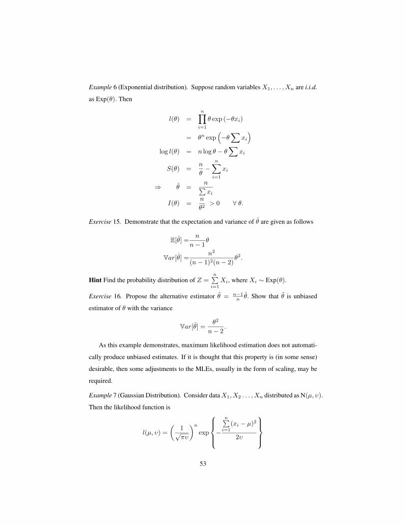
Example 6 (Exponential distribution). Suppose random variablesX1, . . . , Xn are i.i.d.
as Exp(θ). Then
l(θ) =n∏i=1
θ exp (−θxi)
= θn exp(−θ∑
xi
)log l(θ) = n log θ − θ
∑xi
S(θ) =n
θ−
n∑i=1
xi
⇒ θ =n∑xi
I(θ) =n
θ2> 0 ∀ θ.
Exercise 15. Demonstrate that the expectation and variance of θ are given as follows
E[θ] =n
n− 1θ
Var[θ] =n2
(n− 1)2(n− 2)θ2.
Hint Find the probability distribution of Z =n∑i=1
Xi, where Xi ∼ Exp(θ).
Exercise 16. Propose the alternative estimator θ = n−1n θ. Show that θ is unbiased
estimator of θ with the variance
Var[θ] =θ2
n− 2.
As this example demonstrates, maximum likelihood estimation does not automati-
cally produce unbiased estimates. If it is thought that this property is (in some sense)
desirable, then some adjustments to the MLEs, usually in the form of scaling, may be
required.
Example 7 (Gaussian Distribution). Consider dataX1, X2 . . . , Xn distributed as N(µ, υ).
Then the likelihood function is
l(µ, υ) =(
1√πυ
)nexp
−n∑i=1
(xi − µ)2
2υ
53

and the log-likelihood function is
log l(µ, υ) = −n2
log (2π)− n
2log (υ)− 1
2υ
n∑i=1
(xi − µ)2 (3.2)
Unknown mean and known variance As υ is known we treat this parameter as a con-
stant when differentiating wrt µ. Then
S(µ) =1υ
n∑i=1
(xi − µ), µ =1n
n∑i=1
xi, and I(θ) =n
υ> 0 ∀ µ.
Also, E[µ] = nµ/n = µ, and so the MLE of µ is unbiased. Finally
Var[µ] =1n2
Var
[n∑i=1
xi
]=υ
n= (E[I(θ)])−1
.
Known mean and unknown variance Differentiating (3.2) wrt υ returns
S(υ) = − n
2υ+
12υ2
n∑i=1
(xi − µ)2,
and setting S(υ) = 0 implies
υ =1n
n∑i=1
(xi − µ)2.
Differentiating again, and multiplying by −1 yields
I(υ) = − n
2υ2+
1υ3
n∑i=1
(xi − µ)2.
Clearly υ is the MLE since
I(υ) =n
2υ2> 0.
Define
Zi = (Xi − µ)2/√υ,
so that Zi ∼ N(0, 1). From the appendix on probability
n∑i=1
Z2i ∼ χ2
n,
implying E[∑Z2i ] = n, and Var[
∑Z2i ] = 2n. The MLE
υ = (υ/n)n∑i=1
Z2i .
54

Then
E[υ] = E
[υ
n
n∑i=1
Z2i
]= υ,
and
Var[υ] =(υn
)2
Var
[n∑i=1
Z2i
]=
2υ2
n.
2
Our treatment of the two parameters of the Gaussian distribution in the last example
was to (i) fix the variance and estimate the mean using maximum likelihood; and then
(ii) fix the mean and estimate the variance using maximum likelihood. In practice we
would like to consider the simultaneous estimation of these parameters. In the next
section of these notes we extend MLE to multiple parameter estimation.
3.2 Multi-parameter Estimation
Suppose that a statistical model specifies that the data y has a probability distribution
f(y;α, β) depending on two unknown parameters α and β. In this case the likelihood
function is a function of the two variables α and β and having observed the value y is
defined as l(α, β) = f(y;α, β) with log l(α, β) = log l(α, β). The MLE of (α, β) is a
value (α, β) for which l(α, β) , or equivalently log l(α, β) , attains its maximum value.
Define S1(α, β) = ∂ log l/∂α and S2(α, β) = ∂ log l/∂β. The MLEs (α, β) can
be obtained by solving the pair of simultaneous equations
S1(α, β) = 0
S2(α, β) = 0
Let us consider the matrix I(α, β)
I(α, β) =
I11(α, β) I12(α, β)
I21(α, β) I22(α, β)
= −
∂2
∂α2 log l ∂2
∂α∂β log l∂2
∂β∂α log l ∂2
∂β2 log l
The conditions for a value (α0, β0) satisfying S1(α0, β0) = 0 and S2(α0, β0) = 0
to be a MLE are that
I11(α0, β0) > 0, I22(α0, β0) > 0,
55
and
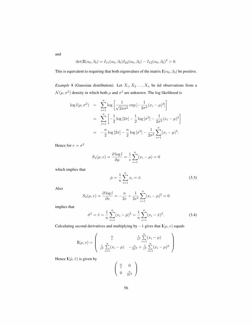
det(I(α0, β0) = I11(α0, β0)I22(α0, β0)− I12(α0, β0)2 > 0.
This is equivalent to requiring that both eigenvalues of the matrix I(α0, β0) be positive.
Example 8 (Gaussian distribution). Let X1, X2 . . . , Xn be iid observations from a
N (µ, σ2) density in which both µ and σ2 are unknown. The log likelihood is
log l(µ, σ2) =n∑i=1
log[
1√2πσ2
exp [− 12σ2
(xi − µ)2]]
=n∑i=1
[−1
2log [2π]− 1
2log [σ2]− 1
2σ2(xi − µ)2
]
= −n2
log [2π]− n
2log [σ2]− 1
2σ2
n∑i=1
(xi − µ)2.
Hence for v = σ2
S1(µ, v) =∂ log l∂µ
=1v
n∑i=1
(xi − µ) = 0
which implies that
µ =1n
n∑i=1
xi = x. (3.3)
Also
S2(µ, v) =∂ log l∂v
= − n
2v+
12v2
n∑i=1
(xi − µ)2 = 0
implies that
σ2 = v =1n
n∑i=1
(xi − µ)2 =1n
n∑i=1
(xi − x)2. (3.4)
Calculating second derivatives and multiplying by −1 gives that I(µ, v) equals
I(µ, v) =
nv
1v2
n∑i=1
(xi − µ)
1v2
n∑i=1
(xi − µ) − n2v2 + 1
v3
n∑i=1
(xi − µ)2
Hence I(µ, v) is given by n
v 0
0 n2v2
56
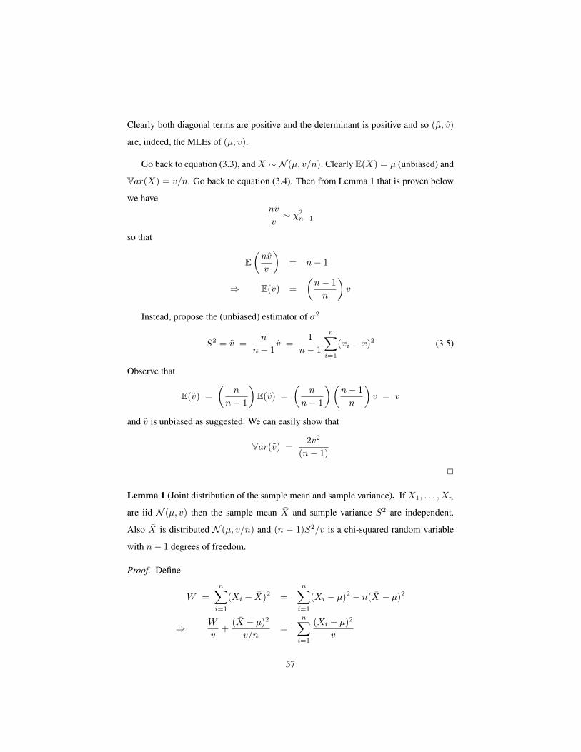
Clearly both diagonal terms are positive and the determinant is positive and so (µ, v)
are, indeed, the MLEs of (µ, v).
Go back to equation (3.3), and X ∼ N (µ, v/n). Clearly E(X) = µ (unbiased) and
Var(X) = v/n. Go back to equation (3.4). Then from Lemma 1 that is proven below
we havenv
v∼ χ2
n−1
so that
E(nv
v
)= n− 1
⇒ E(v) =(n− 1n
)v
Instead, propose the (unbiased) estimator of σ2
S2 = v =n
n− 1v =
1n− 1
n∑i=1
(xi − x)2 (3.5)
Observe that
E(v) =(
n
n− 1
)E(v) =
(n
n− 1
)(n− 1n
)v = v
and v is unbiased as suggested. We can easily show that
Var(v) =2v2
(n− 1)
2
Lemma 1 (Joint distribution of the sample mean and sample variance). If X1, . . . , Xn
are iid N (µ, v) then the sample mean X and sample variance S2 are independent.
Also X is distributed N (µ, v/n) and (n − 1)S2/v is a chi-squared random variable
with n− 1 degrees of freedom.
Proof. Define
W =n∑i=1
(Xi − X)2 =n∑i=1
(Xi − µ)2 − n(X − µ)2
⇒ W
v+
(X − µ)2
v/n=
n∑i=1
(Xi − µ)2
v
57

The RHS is the sum of n independent standard normal random variables squared, and
so is distributed χ2n. Also, X ∼ N (µ, v/n), therefore (X − µ)2/(v/n) is the square
of a standard normal and so is distributed χ21 These Chi-Squared random variables have
moment generating functions (1− 2t)−n/2 and (1− 2t)−1/2 respectively. Next, W/v
and (X − µ)2/(v/n) are independent
Cov(Xi − X, X) = Cov(Xi, X)− Cov(X, X)
= Cov(Xi,
1n
∑Xj
)− Var(X)
=1n
∑j
Cov(Xi, Xj)−v
n
=v
n− v
n= 0
But, Cov(Xi − X, X − µ) = Cov(Xi − X, X) = 0 , hence
∑i
Cov(Xi − X, X − µ) = Cov
(∑i
(Xi − X), X − µ
)= 0
As the moment generating function of the sum of independent random variables is
equal to the product of their individual moment generating functions, we see
E[et(W/v)
](1− 2t)−1/2 = (1− 2t)−n/2
⇒ E[et(W/v)
]= (1− 2t)−(n−1)/2
But (1−2t)−(n−1)/2 is the moment generating function of a χ2 random variables with
(n−1) degrees of freedom, and the moment generating function uniquely characterizes
the random variable S = (W/v).
Suppose that a statistical model specifies that the data x has a probability distri-
bution f(x; θ) depending on a vector of m unknown parameters θ = (θ1, . . . , θm).
In this case the likelihood function is a function of the m parameters θ1, . . . , θm and
having observed the value of x is defined as l(θ) = f(x; θ) with log l(θ) = log l(θ).
The MLE of θ is a value θ for which l(θ), or equivalently log l(θ), attains its
maximum value. For r = 1, . . . ,m define Sr(θ) = ∂ log l/∂θr. Then we can (usually)
find the MLE θ by solving the set of m simultaneous equations Sr(θ) = 0 for r =
58

1, . . . ,m. The matrix I(θ) is defined to be the m ×m matrix whose (r, s) element is
given by Irs where Irs = −∂2 log l/∂θr∂θs. The conditions for a value θ satisfying
Sr(θ) = 0 for r = 1, . . . ,m to be a MLE are that all the eigenvalues of the matrix I(θ)
are positive.
3.3 The Invariance Principle
How do we deal with parameter transformation? We will assume a one-to-one trans-
formation, but the idea applied generally. Consider a binomial sample with n = 10
independent trials resulting in data x = 8 successes. The likelihood ratio of θ1 = 0.8
versus θ2 = 0.3 isl(θ1 = 0.8)l(θ2 = 0.3)
=θ8
1(1− θ1)2
θ82(1− θ2)2
= 208.7 ,
that is, given the data θ = 0.8 is about 200 times more likely than θ = 0.3.
Suppose we are interested in expressing θ on the logit scale as
ψ ≡ logθ/(1− θ) ,
then ‘intuitively’ our relative information about ψ1 = log(0.8/0.2) = 1.29 versus
ψ2 = log(0.3/0.7) = −0.85 should be
L∗(ψ1)L∗(ψ2)
=l(θ1)l(θ2)
= 208.7 .
That is, our information should be invariant to the choice of parameterization. ( For
the purposes of this example we are not too concerned about how to calculate L∗(ψ). )
Theorem 3.3.1 (Invariance of the MLE). If g is a one-to-one function, and θ is the
MLE of θ then g(θ) is the MLE of g(θ).
Proof. This is trivially true as we let θ = g−1(µ) then fy|g−1(µ) is maximized in µ
exactly when µ = g(θ).When g is not one-to-one the discussion becomes more subtle,
but we simply choose to define gMLE(θ) = g(θ)
It seems intuitive that if θ is most likely for θ and our knowledge (data) remains
unchanged then g(θ) is most likely for g(θ). In fact, we would find it strange if θ is an
59

estimate of θ, but θ2 is not an estimate of θ2. In the binomial example with n = 10 and
x = 8 we get θ = 0.8, so the MLE of g(θ) = θ/(1− θ) is
g(θ) = θ/(1− θ) = 0.8/0.2 = 4.
60

Chapter 4
Estimation
In the previous chapter we have seen an approach to estimation that is based on the
likelihood of observed results. Next we study general theory of estimation that is used
to compare between different estimators and to decide on the most efficient one.
4.1 General properties of estimators
Suppose that we are going to observe a value of a random vector X. Let X denote the
set of possible values X can take and, for x ∈ X , let f(x|θ) denote the probability that
X takes the value x where the parameter θ is some unknown element of the set Θ.
The problem we face is that of estimating θ. An estimator θ is a procedure which
for each possible value x ∈ X specifies which element of Θ we should quote as an
estimate of θ. When we observe X = x we quote θ(x) as our estimate of θ. Thus θ is
a function of the random vector X. Sometimes we write θ(X) to emphasise this point.
Given any estimator θ we can calculate its expected value for each possible value
of θ ∈ Θ. As we have already mentioned when discussing the maximum likelihood
estimation, an estimator is said to be unbiased if this expected value is identically equal
to θ. If an estimator is unbiased then we can conclude that if we repeat the experiment
an infinite number of times with θ fixed and calculate the value of the estimator each
time then the average of the estimator values will be exactly equal to θ. To evaluate
61

the usefulness of an estimator θ = θ(x) of θ, examine the properties of the random
variable θ = θ(X).
Definition 1 (Unbiased estimators). An estimator θ = θ(X) is said to be unbiased for
a parameter θ if it equals θ in expectation
E[θ(X)] = E(θ) = θ.
Intuitively, an unbiased estimator is ‘right on target’. 2
Definition 2 (Bias of an estimator). The bias of an estimator θ = θ(X) of θ is defined
as bias(θ) = E[θ(X)− θ]. 2
Note that even if θ is an unbiased estimator of θ, g(θ) will generally not be an
unbiased estimator of g(θ) unless g is linear or affine. This limits the importance of the
notion of unbiasedness. It might be at least as important that an estimator is accurate
in the sense that its distribution is highly concentrated around θ.
Exercise 17. Show that for an arbitrary distribution the estimator S2 as defined in (3.5)
is an unbiased estimator of the variance of this distribution.
Exercise 18. Consider the estimator S2 of variance σ2 in the case of the normal dis-
tribution. Demonstrate that although S2 is an unbiased estimator of σ2, S is not an
unbiased estimator of σ. Compute its bias.
Definition 3 (Mean squared error). The mean squared error of the estimator θ is de-
fined as MSE(θ) = E(θ − θ)2. Given the same set of data, θ1 is “better” than θ2 if
MSE(θ1) ≤ MSE(θ2) (uniformly better if true ∀ θ). 2
Lemma 2 (The MSE variance-bias tradeoff). The MSE decomposes as
MSE(θ) = Var(θ) + bias(θ)2.
62

Proof. We have
MSE(θ) = E(θ − θ)2
= E [ θ − E(θ) ] + [ E(θ)− θ ]2
= E[θ − E(θ)]2 + E[E(θ)− θ]2
+2 E
[θ − E(θ)][E(θ)− θ]
︸ ︷︷ ︸=0
= E[θ − E(θ)]2 + E[E(θ)− θ]2
= Var(θ) + [E(θ)− θ]2︸ ︷︷ ︸bias(θ)
2
.
NOTE This lemma implies that the mean squared error of an unbiased estimator is
equal to the variance of the estimator.
Exercise 19. Consider X1, . . . , Xn where Xi ∼ N(θ, σ2) and σ is known. Three
estimators of θ are θ1 = X = 1n
∑ni=1Xi, θ2 = X1, and θ3 = (X1 + X)/2. Discuss
their properties which one you would recommend and why.
Example 9. Consider X1, . . . , Xn to be independent random variables with means
E(Xi) = µ and variances Var(Xi) = σ2i . Consider pooling the estimators of µ into a
common estimator using the linear combination µ = w1X1 + w2X2 + · · · + wnXn.
We will see that the following is true
(i) The estimator µ is unbiased if and only if∑wi = 1.
(ii) The estimator µ has minimum variance among this class of estimators when the
weights are inversely proportional to the variances σ2i .
(iii) The variance of µ for optimal weights wi is Var(µ) = 1/∑i σ−2i .
Indeed, we have E(µ) = E(w1X1 + · · · + wnXn) =∑i wiE(Xi) =
∑i wiµ =
µ∑i wi so µ is unbiased if and only if
∑i wi = 1. The variance of our estimator is
Var(µ) =∑i w
2i σ
2i , which should be minimized subject to the constraint
∑i wi = 1.
Differentiating the Lagrangian L =∑i w
2i σ
2i − λ (
∑i wi − 1) with respect to wi and
63

setting equal to zero yields 2wiσ2i = λ ⇒ wi ∝ σ−2
i so that wi = σ−2i /(
∑j σ−2j ).
Then, for optimal weights we get Var(µ) =∑i w
2i σ
2i = (
∑i σ−4i σ2
i )/(∑i σ−2i )2 =
1/(∑i σ−2i ).
Assume now that the instead of Xi we observe biased variable Xi = Xi + β for
some β 6= 0. When σ2i = σ2 we have that Var(µ) = σ2/n which tends to zero for
n → ∞ whereas bias(µ) = βand MSE(µ) = σ2/n + β2. Thus in the general case
when the bias is present it tends to dominate the variance as n gets larger, which is very
unfortunate.
Exercise 20. Let X1, . . . , Xn be an independent sample of size n from the uniform
distribution on the interval (0, θ), with density for a single observation being f(x|θ) =
θ−1 for 0 < x < θ and 0 otherwise, and consider θ > 0 unknown.
(i) Find the expected value and variance of the estimator θ = 2X.
(ii) Find the expected value of the estimator θ = X(n), i.e. the largest observation.
(iii) Find an unbiased estimator of the form θ = cX(n) and calculate its variance.
(iv) Compare the mean square error of θ and θ.
4.2 Minimum-Variance Unbiased Estimation
Getting a small MSE often involves a tradeoff between variance and bias. For unbiased
estimators, the MSE obviously equals the variance, MSE(θ) = Var(θ), so no tradeoff
can be made. One approach is to restrict ourselves to the subclass of estimators that are
unbiased and minimum variance.
Definition 4 (Minimum-variance unbiased estimator). If an unbiased estimator of g(θ)
has minimum variance among all unbiased estimators of g(θ) it is called a minimum
variance unbiased estimator (MVUE). 2
We will develop a method of finding the MVUE when it exists. When such an
estimator does not exist we will be able to find a lower bound for the variance of an
unbiased estimator in the class of unbiased estimators, and compare the variance of our
unbiased estimator with this lower bound.
64
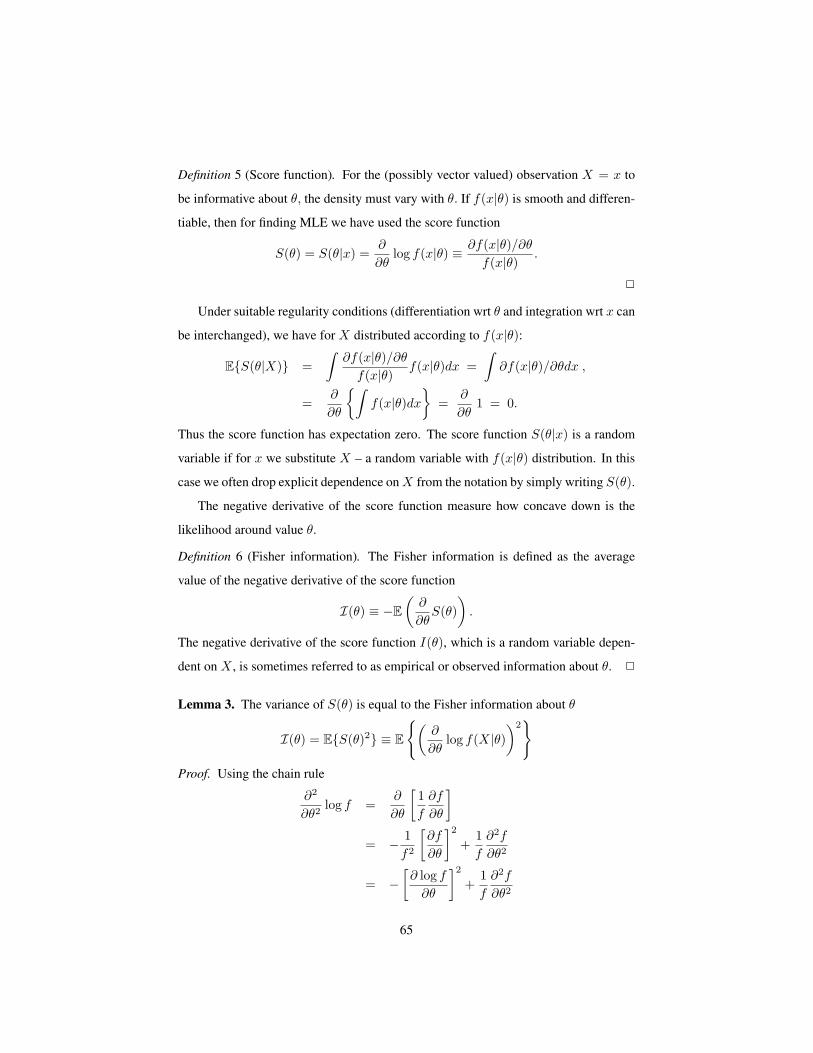
Definition 5 (Score function). For the (possibly vector valued) observation X = x to
be informative about θ, the density must vary with θ. If f(x|θ) is smooth and differen-
tiable, then for finding MLE we have used the score function
S(θ) = S(θ|x) =∂
∂θlog f(x|θ) ≡ ∂f(x|θ)/∂θ
f(x|θ).
2
Under suitable regularity conditions (differentiation wrt θ and integration wrt x can
be interchanged), we have for X distributed according to f(x|θ):
ES(θ|X) =∫∂f(x|θ)/∂θf(x|θ)
f(x|θ)dx =∫∂f(x|θ)/∂θdx ,
=∂
∂θ
∫f(x|θ)dx
=
∂
∂θ1 = 0.
Thus the score function has expectation zero. The score function S(θ|x) is a random
variable if for x we substitute X – a random variable with f(x|θ) distribution. In this
case we often drop explicit dependence onX from the notation by simply writing S(θ).
The negative derivative of the score function measure how concave down is the
likelihood around value θ.
Definition 6 (Fisher information). The Fisher information is defined as the average
value of the negative derivative of the score function
I(θ) ≡ −E(∂
∂θS(θ)
).
The negative derivative of the score function I(θ), which is a random variable depen-
dent on X , is sometimes referred to as empirical or observed information about θ. 2
Lemma 3. The variance of S(θ) is equal to the Fisher information about θ
I(θ) = ES(θ)2 ≡ E
(∂
∂θlog f(X|θ)
)2
Proof. Using the chain rule
∂2
∂θ2log f =
∂
∂θ
[1f
∂f
∂θ
]= − 1
f2
[∂f
∂θ
]2
+1f
∂2f
∂θ2
= −[∂ log f∂θ
]2
+1f
∂2f
∂θ2
65

If integration and differentiation can be interchanged
E[
1f
∂2f
∂θ2
]=∫X
∂2f
∂θ2dx =
∂2
∂θ2
∫X
fdx =∂2
∂θ21 = 0,
thus
− E[∂2
∂θ2log f(X|θ)
]= E
[(∂
∂θlog f(X|θ)
)2]
= I(θ). (4.1)
Theorem 4.2.1 (Cramer Rao lower bound). Let θ be an unbiased estimator of θ. Then
Var(θ) ≥ I(θ) −1.
Proof. Unbiasedness, E(θ) = θ, implies∫θ(x)f(x|θ)dx = θ.
Assume we can differentiate wrt θ under the integral, then∫∂
∂θ
θ(x)f(x|θ)
dx = 1.
The estimator θ(x) can’t depend on θ, so∫θ(x)
∂
∂θf(x|θ) dx = 1.
Since∂f
∂θ= f
∂
∂θ(log f) ,
so that now ∫θ(x)f
∂
∂θ(log f) dx = 1.
Thus
E[θ(x)
∂
∂θ(log f)
]= 1.
Define random variables
U = θ(x),
and
S =∂
∂θ(log f) .
66

Then E (US) = 1. We already know that the score function has expectation zero,
E (S) = 0. Consequently Cov(U, S) = E(US) − E(U)E(S) = E(US) = 1. By the
well-known property of correlations (that follows from the Schwartz’s inequality) we
have
Corr(U, S)2 =Cov(U, S)2
Var(U)Var(S)≤ 1
Since, as we mentioned, Cov(U, S) = 1 we get
Var(U)Var(S) ≥ 1
This implies
Var(θ) ≥ 1I(θ)
which is our main result. We call I(θ) −1 the Cramer Rao lower bound (CRLB).
Why information? Variance measures lack of knowledge. Reasonable that the
reciprocal of the variance should be defined as the amount of information carried by
the (possibly vector valued) random observation X about θ.
Sufficient conditions for the proof of CRLB are that all the integrands are finite,
within the range of x. We also require that the limits of the integrals do not depend on
θ. That is, the range of x, here f(x|θ), cannot depend on θ. This second condition is
violated for many density functions, i.e. the CRLB is not valid for the uniform distri-
bution. We can have absolute assessment for unbiased estimators by comparing their
variances to the CRLB. We can also assess biased estimators. If its variance is lower
than CRLB then it can be indeed a very good estimate, although it is bias.
Example 10. Consider IID random variables Xi, i = 1, . . . , n, with
fXi(xi|µ) =1µ
exp(− 1µxi
).
Denote the joint distribution of X1, . . . , Xn by
f =n∏i=1
fXi(xi|µ) =(
1µ
)nexp
(− 1µ
n∑i=1
xi
),
so that
log f = −n log(µ)− 1µ
n∑i=1
xi.
67

The score function is the partial derivative of log f wrt the unknown parameter µ,
S(µ) =∂
∂µlog f = −n
µ+
1µ2
n∑i=1
xi
and
E S(µ) = E
−nµ
+1µ2
n∑i=1
Xi
= −n
µ+
1µ2
E
n∑i=1
Xi
For X ∼ Exp(1/µ), we have E(X) = µ implying E(X1 + · · · + Xn) = E(X1) +
· · ·+ E(Xn) = nµ and E S(µ) = 0 as required.
I(θ) = −E
∂
∂µ
(−nµ
+1µ2
n∑i=1
Xi
)
= −E
n
µ2− 2µ3
n∑i=1
Xi
= − n
µ2+
2µ3
E
n∑i=1
Xi
= − n
µ2+
2nµµ3
=n
µ2
Hence
CRLB =µ2
n.
Let us propose µ = X as an estimator of µ. Then
E(µ) = E
1n
n∑i=1
Xi
=
1n
E
n∑i=1
Xi
= µ,
verifying that µ = X is indeed an unbiased estimator of µ. For X ∼ Exp(1/µ), we
have E(X) = µ =√
Var(X), implying
Var(µ) =1n2
n∑i=1
Var(Xi) =nµ2
n2=µ2
n.
We have already shown that Var(µ) = I(θ) −1, and therefore conclude that the
unbiased estimator µ = x achieves its CRLB. 2
Definition 7 (Efficiency ). Define the efficiency of the unbiased estimator θ as
eff(θ) =CRLB
Var(θ),
68

where CRLB = I(θ) −1. Clearly 0 < eff(θ) ≤ 1. An unbiased estimator θ is said
to be efficient if eff(θ) = 1. 2
Exercise 21. Consider the MLE θ = r/n for the binomial distribution that was con-
sidered in Example 3. Show that for this estimator efficiency is 100%, i.e. its variance
attains CRLB.
Exercise 22. Consider the MLE for the Poisson distribution that was considered in
Example 5. Show that also in this case the MLE is 100% efficient.
Definition 8 (Asymptotic efficiency ). The asymptotic efficiency of an unbiased esti-
mator θ is the limit of the efficiency as n → ∞. An unbiased estimator θ is said to be
asymptotically efficient if its asymptotic efficiency is equal to 1. 2
Exercise 23. Consider the MLE θ for the exponential distribution with parameter θ that
was considered in Exercise 16. Find its variance, and its mean square error. Consider
also θ that was considered in this example. Which of the two has smaller variance and
which has smaller mean square error? Is θ asymptotically efficient?
Exercise 24. Discuss efficiency of the estimator of variance in the normal distribution
in the case when the mean is known (see Example 7).
4.3 Optimality Properties of the MLE
Suppose that an experiment consists of measuring random variables X1, X2, . . . , Xn
which are iid with probability distribution depending on a parameter θ. Let θ be the
MLE of θ. Define
W1 =√I(θ)(θ − θ)
W2 =√I(θ)(θ − θ)
W3 =√I(θ)(θ − θ)
W4 =√I(θ)(θ − θ).
Then, W1,W2,W3, and W4 are all random variables and, as n→∞, the probabilistic
behaviour of each of W1,W2,W3, and W4 is well approximated by that of a N(0, 1)
random variable.
69

Since E[W1] ≈ 0, we have that E[θ] ≈ θ and so θ is approximately unbiased. Also
Var[W1] ≈ 1 implies that Var[θ] ≈ (I(θ))−1 and so θ is asymptotically efficient. The
above properties of the MLE estimators carry to the multivariate case. Here is a brief
account of these properties.
Let the data X have probability distribution g(X;θθθ) where θθθ = (θ1, θ2, . . . , θm) is
a vector of m unknown parameters.
Let I(θθθ) be the m × m observed information matrix and let I(θθθ) be the m ×
m Fisher’s information matrix obtained by replacing the elements of I(θθθ) by their
expected values. Let θθθ be the MLE of θθθ. LetCRLBr be the rth diagonal element of the
Fisher’s information matrix. For r = 1, 2, . . . ,m, define W1r = (θr − θr)/√CRLBr.
Then, as n→∞,W1r behaves like a standard normal random variable.
Suppose we define W2r by replacing CRLBr by the rth diagonal element of the
matrix I(θθθ)−1,W3r by replacing CRLBr by the rth diagonal element of the matrix
I(θθθ)−1 and W4r by replacing CRLBr by the rth diagonal element of the matrix
I(θθθ)−1. Then it can be shown that as n → ∞,W2r,W3r, and W4r all behave like
standard normal random variables.
70
Chapter 5
The Theory of Confidence
Intervals
5.1 Exact Confidence Intervals
Suppose that we are going to observe the value of a random vector X. LetX denote the
set of possible values that X can take and, for x ∈ X , let g(x|θ) denote the probability
that X takes the value x where the parameter θ is some unknown element of the set Θ.
Consider the problem of quoting a subset of θ values which are in some sense plausible
in the light of the data x. We need a procedure which for each possible value x ∈ X
specifies a subset C(x) of Θ which we should quote as a set of plausible values for θ.
Definition 9. Let X1, . . . , Xn be a sample form a distribution that is parameterized
by some parameter θ. A random set C(X1, . . . , Xn) of possible values for θ that is
computable from the sample is called a confidence region at confidence level 1− α if
P(θ ∈ C(X1, . . . , Xn)) = 1− α.
If the set C(X1, . . . , Xn) has the form of an interval, then we call it a confidence
interval.
Example 11. Suppose we are going to observe data x where x = (x1, x2, . . . , xn), and
71
x1, x2, . . . , xn are the observed values of random variables X1, X2, . . . , Xn which are
thought to be iid N(θ, 1) for some unknown parameter θ ∈ (−∞,∞) = Θ. Consider
the subset C(x) = [x− 1.96/√n, x+ 1.96/
√n]. If we carry out an infinite sequence
of independent repetitions of the experiment then we will get an infinite sequence of x
values and thereby an infinite sequence of subsetsC(x). We might ask what proportion
of this infinite sequence of subsets actually contain the fixed but unknown value of θ?
Since C(x) depends on x only through the value of x we need to know how x
behaves in the infinite sequence of repetitions. This follows from the fact that X has a
N(θ, 1n ) density and so Z = X−θ
1√n
=√n(X − θ) has a N(0, 1) density. Thus even-
though θ is unknown we can calculate the probability that the value of Z will exceed
2.78, for example, using the standard normal tables. Remember that the probability is
the proportion of experiments in the infinite sequence of repetitions which produce a
value of Z greater than 2.78.
In particular we have that P [|Z| ≤ 1.96] = 0.95. Thus 95% of the time Z will lie
between −1.96 and +1.96. But
−1.96 ≤ Z ≤ +1.96 ⇒ −1.96 ≤√n(X − θ) ≤ +1.96
⇒ −1.96/√n ≤ X − θ ≤ +1.96/
√n
⇒ X − 1.96/√n ≤ θ ≤ X + 1.96/
√n
⇒ θ ∈ C(X)
Thus we have answered the question we started with. The proportion of the infinite se-
quence of subsets given by the formula C(X) which will actually include the fixed but
unknown value of θ is 0.95. For this reason the set C(X) is called a 95% confidence
set or confidence interval for the parameter θ. 2
It is well to bear in mind that once we have actually carried out the experiment and
observed our value of x, the resulting interval C(x) either does or does not contain
the unknown parameter θ. We do not know which is the case. All we know is that the
procedure we used in constructing C(x) is one which 95% of the time produces an
interval which contains the unknown parameter.
72

0 20 40 60 80 100
510
1520
25
Index
c(0,
mu)
Figure 5.1: One hundred confidence intervals for the mean of a normal variable with
“unknown” mean and variance for sample size of ten. In fact the samples have been
drawn from the normal distribution with the mean 15 and standard deviation 6.
The crucial step in the last example was finding the quantity Z =√n(X − θ)
whose value depended on the parameter of interest θ but whose distribution was known
to be that of a standard normal variable. This leads to the following definition.
Definition 10 (Pivotal Quantity). A pivotal quantity for a parameter θ is a random
variable Q(X|θ) whose value depends both on (the data) X and on the value of the
unknown parameter θ but whose distribution is known. 2
The quantity Z in the example above is a pivotal quantity for θ. The following
lemma provides a method of finding pivotal quantities in general.
Lemma 4. Let X be a random variable and define F (a) = P [X ≤ a]. Consider the
random variable U = −2 log [F (X)]. Then U has a χ22 density. Consider the random
variable V = −2 log [1− F (X)]. Then V has a χ22 density.
73

Proof. Observe that, for a ≥ 0,
P [U ≤ a] = P [F (X) ≥ exp (−a/2)]
= 1− P [F (X) ≤ exp (−a/2)]
= 1− P [X ≤ F−1(exp (−a/2))]
= 1− F [F−1(exp (−a/2))]
= 1− exp (−a/2).
Hence, U has density 12 exp (−a/2) which is the density of a χ2
2 variable as required.
The corresponding proof for V is left as an exercise.
This lemma has an immediate, and very important, application.
Suppose that we have data X1, X2, . . . , Xn which are iid with density f(x|θ). De-
fine F (a|θ) =∫ a−∞ f(x|θ)dx and, for i = 1, 2, . . . , n, define Ui = −2 log[F (Xi|θ)].
ThenU1, U2, . . . , Un are iid each having a χ22 density. HenceQ1(X, θ) =
∑ni=1 Ui has
a χ22n density and so is a pivotal quantity for θ. Another pivotal quantity ( also having
a χ22n density ) is given by Q2(X, θ) =
∑ni=1 Vi where Vi = −2 log[1− F (Xi|θ)].
Example 12. Suppose that we have data X1, X2, . . . , Xn which are iid with density
f(x|θ) = θ exp (−θx)
for x ≥ 0 and suppose that we want to construct a 95% confidence interval for θ. We
need to find a pivotal quantity for θ. Observe that
F (a|θ) =∫ a
−∞f(x|θ)dx
=∫ a
0
θ exp (−θx)dx
= 1− exp (−θa).
Hence
Q1(X, θ) = −2n∑i=1
log [1− exp (−θXi)]
is a pivotal quantity for θ having a χ22n density. Also
Q2(X, θ) = −2n∑i=1
log [exp (−θXi)] = 2θn∑i=1
Xi
74

is another pivotal quantity for θ having a χ22n density.
Using the tables, find A < B such that P [χ22n < A] = P [χ2
2n > B] = 0.025.
Then
0.95 = P [A ≤ Q2(X, θ) ≤ B]
= P [A ≤ 2θn∑i=1
Xi ≤ B]
= P [A
2∑ni=1Xi
≤ θ ≤ B
2∑ni=1Xi
]
and so the interval
[A
2∑ni=1Xi
,B
2∑ni=1Xi
]
is a 95% confidence interval for θ.
5.2 Pivotal Quantities for Use with Normal Data
Many exact pivotal quantities have been developed for use with Gaussian data.
Exercise 25. Suppose that we have data X1, X2, . . . , Xn which are iid observations
from a N (θ, σ2) density where σ is known. Define
Q =√n(X − θ)σ
.
Show that the defined random variable is pivotal for µ. Construct confidence intervals
for µ based on this pivotal quantity.
Example 13. Suppose that we have data X1, X2, . . . , Xn which are iid observations
from a N(θ, σ2) density where θ is known. Define
Q =
n∑i=1
(Xi − θ)2
σ2
We can write Q =n∑i=1
Z2i where Zi = (Xi − θ)/σ. If Zi has a N (0, 1) density then
Z2i has a χ2
1 density. Hence, Q has a χ2n density and so is a pivotal quantity for σ. If
n = 20 then we can be 95% sure that
9.591 ≤
n∑i=1
(Xi − θ)2
σ2≤ 34.170
75

which is equivalent to√√√√ 134.170
n∑i=1
(Xi − θ)2 ≤ σ ≤
√√√√ 19.591
n∑i=1
(Xi − θ)2.
The R command qchisq(p=c(.025,.975),df=20) returns the values 9.590777
and 34.169607 as the 2 12 % and 97 1
2 % quantiles from a Chi-squared distribution on 20
degrees of freedom. 2
Lemma 5 (The Student t-distribution). Suppose the random variables X and Y are
independent, and X ∼ N(0, 1) and Y ∼ χ2n. Then the ratio
T =X√Y/n
has pdf
fT (t|n) =1√πn
Γ([n+ 1]/2)Γ(n/2)
(1 +
t2
n
)−(n+1)/2
,
and is known as Student’s t-distribution on n degrees of freedom.
Proof. The random variables X and Y are independent and have joint density
fX,Y (x, y) =1√2π
2−n/2
Γ(n/2)e−x
2/2yn/2−1e−y/2−1e−y/2 for y > 0.
The Jacobian ∂(t, u)/∂(x, y) of the change of variables
t =x√y/n
and u = y
equals
∂(t, u)∂(x, y)
≡
∣∣∣∣∣∣∂t∂x
∂t∂y
∂u∂x
∂u∂y
∣∣∣∣∣∣ =
∣∣∣∣∣∣√n/y − 1
2x√n
(y)3/2
0 1
∣∣∣∣∣∣ = (n/y)1/2
and the inverse Jacobian
∂(x, y)/∂(t, u) = (u/n)1/2.
76

Then
fT (t) =∫ ∞
0
fX,Y
(t(u/n)1/2, u
)(un
)1/2
du
=1√2π
2−n/2
Γ(n/2)
∫ ∞0
e−t2u/2nun/2−1e−u/2
(un
)1/2
du
=1√2π
2−n/2
Γ(n/2)n1/2
∫ ∞0
e−(1+t2/n)u/2u(n+1)/2−1du .
The last integrand comes from the pdf of a Gam((n + 1)/2, 1/2 + t2/(2n)) random
variable. Hence
fT (t) =1√πn
Γ([n+ 1]/2)Γ(n/2)
(1
1 + t2/n
)(n+1)/2
,
which gives the above formula.
Example 14. Suppose that we have data X1, X2, . . . , Xn which are iid observations
from a N (θ, σ2) density where both θ and σ are unknown. Define
Q =√n(X − θ)
s
where
s2 =
n∑i=1
(Xi − X)2
n− 1.
We can write
Q =Z√
W/(n− 1)
where
Z =√n(X − θ)σ
has a N (0, 1) density and
W =
n∑i=1
(Xi − X)2
σ2
has a χ2n−1 density ( see lemma 1 ). It follows immediately that W is a pivotal quantity
for σ. If n = 31 then we can be 95% sure that
16.79077 ≤
n∑i=1
(Xi − X)2
σ2≤ 46.97924
77

which is equivalent to√√√√ 146.97924
n∑i=1
(Xi − X)2 ≤ σ ≤
√√√√ 116.79077
n∑i=1
(Xi − X)2. (5.1)
The R command qchisq(p=c(.025,.975),df=30) returns the values 16.79077
and 46.97924 as the 2 12 % and 97 1
2 % quantiles from a Chi-squared distribution on 30
degrees of freedom. In lemma 5 we show that Q has a tn−1 density, and so is a pivotal
quantity for θ. If n = 31 then we can be 95% sure that
−2.042 ≤√n(X − θ)
s≤ +2.042
which is equivalent to
X − 2.042s√n≤ θ ≤ X + 2.042
s√n. (5.2)
The R command qt(p=.975,df=30) returns the value 2.042272 as the 97 12 % quan-
tile from a Student t-distribution on 30 degrees of freedom. ( It is important to point
out that although a probability statement involving 95% confidence has been attached
the two intervals (5.2) and (5.1) separately, this does not imply that both intervals si-
multaneously hold with 95% confidence. ) 2
Example 15. Suppose that we have data X1, X2, . . . , Xn which are iid observations
from a N (θ1, σ2) density and data Y1, Y2, . . . , Ym which are iid observations from a
N (θ2, σ2) density where θ1, θ2, and σ are unknown. Let δ = θ1 − θ2 and define
Q =(X − Y )− δ√s2( 1
n + 1m )
where
s2 =
∑ni=1(Xi − X)2 +
∑mj=1(Yj − Y )2
n+m− 2.
We know that X has a N (θ1,σ2
n ) density and that Y has a N (θ2,σ2
m ) density. Then
the difference X − Y has a N (δ, σ2[ 1n + 1
m ]) density. Hence
Z =X − Y − δ√σ2[ 1
n + 1m ]
78

has a N (0, 1) density. Let W1 =∑ni=1(Xi − X)2/σ2 and let W2 =
∑mj=1(Yj −
Y )2/σ2. Then,W1 has a χ2n−1 density andW2 has a χ2
m−1 density, andW = W1+W2
has a χ2n+m−2 density. We can write
Q1 = Z/√W/(n+m− 2)
and so, Q1 has a tn+m−2 density and so is a pivotal quantity for δ. Define
Q2 =
∑ni=1(Xi − X)2 +
∑mj=1(Yj − Y )2
σ2.
Then Q2 has a χ2n+m−2 density and so is a pivotal quantity for σ. 2
Lemma 6 (The Fisher F-distribution). Let X1, X2, . . . , Xn and Y1, Y2, . . . , Ym be iid
N (0, 1) random variables. The ratio
Z =
n∑i=1
X2i /n
m∑i=1
Y 2i /m
has the distribution called Fisher, or F distribution with parameters (degrees of free-
dom) n,m, or the Fn,m distribution for short. The corresponding pdf fFn,m is concen-
trated on the positive half axis
fFn,m(z) =Γ((n+m)/2)Γ(n/2)Γ(m/2)
( nm
)n/2zn/2−1
(1 +
n
mz)−(n+m)/2
for z > 0.
Observe that if T ∼ tm, then T 2 = Z ∼ F1,m, and if Z ∼ Fn,m, then Z−1 ∼ Fm,n.
If W1 ∼ χ2n and W2 ∼ χ2
m, then Z = (mW1)/(nW2) ∼ Fn,m. 2
Example 16. Suppose that we have data X1, X2, . . . , Xn which are iid observations
from a N (θX , σ2X) density and data Y1, Y2, . . . , Ym which are iid observations from a
N (θY , σ2Y ) density where θX , θY , σX , and σY are all unknown. Let
λ = σX/σY
and define
F ∗ =s2X
s2Y
=∑ni=1(Xi − X)2
(n− 1)(m− 1)∑m
j=1(Yj − Y )2.
79

Let
WX =n∑i=1
(Xi − X)2/σ2X
and let
WY =m∑j=1
(Yj − Y )2/σ2Y .
Then, WX has a χ2n−1 density and WY has a χ2
m−1 density. Hence, by lemma 6,
Q =WX/(n− 1)WY /(m− 1)
≡ F ∗
λ2
has an F density with n−1 andm−1 degrees of freedom and so is a pivotal quantity for
λ. Suppose that n = 25 and m = 13. Then we can be 95% sure that 0.39 ≤ Q ≤ 3.02
which is equivalent to √F ∗
3.02≤ λ ≤
√F ∗
0.39.
To see how this might work in practice try the following R commands one at a time
x = rnorm(25, mean = 0, sd = 2)
y = rnorm(13, mean = 1, sd = 1)
Fstar = var(x)/var(y); Fstar
CutOffs = qf(p=c(.025,.975), df1=24, df2=12)
CutOffs; rev(CutOffs)
Fstar / rev(CutOffs)
var.test(x, y)
2
The search for a nice pivotal quantity for δ = θ1 − δ2 continues and is one of the
unsolved problems in Statistics - referred to as the Behrens-Fisher Problem.
5.3 Approximate Confidence Intervals
Let X1, X2, . . . , Xn be iid with density f(x|θ). Let θ be the MLE of θ. We saw before
that the quantities W1 =√I(θ)(θ − θ),W2 =
√I(θ)(θ − θ),W3 =
√I(θ)(θ −
θ), and W4 =√I(θ)(θ − θ) all had densities which were approximately N (0, 1).
80

Hence they are all approximate pivotal quantities for θ. W3 and W4 are the simplest
to use in general. For W3 the approximate 95% confidence interval is given by [θ −
1.96/√I(θ), θ + 1.96/
√I(θ)]. For W4 the approximate 95% confidence interval is
given by [θ − 1.96/√I(θ), θ + 1.96/
√I(θ)]. The quantity 1/
√I(θ) ( or 1/
√I(θ))
is often referred to as the approximate standard error of the MLE θ.
Let X1, X2, . . . , Xn be iid with density f(x|θ) where θ = (θ1, θ2, . . . , θm) con-
sists of m unknown parameters. Let θ = (θ1, θ2, . . . , θm) be the MLE of θ. We saw
before that for r = 1, 2, . . . ,m the quantities W1r = (θr − θr)/√CRLBr where
CRLBr is the lower bound for Var(θr) given in the generalisation of the Cramer-Rao
theorem had a density which was approximately N (0, 1). Recall that CRLBr is the
rth diagonal element of the matrix [I(θ)]−1. In certain cases CRLBr may depend on
the values of unknown parameters other than θr and in those cases W1r will not be an
approximate pivotal quantity for θr.
We also saw that if we define W2r by replacing CRLBr by the rth diagonal ele-
ment of the matrix [I(θ)]−1,W3r by replacing CRLBr by the rth diagonal element
of the matrix [I(θ)]−1 and W4r by replacing CRLBr by the rth diagonal element of
the matrix [I(θ)]−1 we get three more quantities all of whom have a density which is
approximately N (0, 1). W3r and W4r only depend on the unknown parameter θr and
so are approximate pivotal quantities for θr. However in certain cases the rth diago-
nal element of the matrix [I(θ)]−1 may depend on the values of unknown parameters
other than θr and in those cases W2r will not be an approximate pivotal quantity for
θr. Generally W3r and W4r are most commonly used.
We now examine the use of approximate pivotal quantities based on the MLE in a
series of examples
Example 17 (Poisson sampling continued). Recall that θ = x and I(θ) =∑ni=1 xi/θ
2 =
nθ/θ2 with E[I(θ)] = n/θ. Hence I(θ) = I(θ) = n/θ and the usual approximate
95% confidence interval is given by
[ θ − 1.96
√θ
n, θ + 1.96
√θ
n].
2
81

Example 18 (Bernoulli trials continued). Recall that θ = x and
I(θ) =∑ni=1 xiθ2
+n−
∑ni=1 xi
(1− θ)2
with
I(θ) = EI(θ) =n
θ(1− θ).
Hence
I(θ) = I(θ) =n
θ(1− θ)and the usual approximate 95% confidence interval is given by
[ θ − 1.96
√θ(1− θ)
n, θ + 1.96
√θ(1− θ)
n].
2
Example 19. Let X1, X2, . . . , Xn be iid observations from the density
f(x|α, β) = αβxβ−1 exp [−αxβ ]
for x ≥ 0 where both α and β are unknown. In can be verified by straightforward
calculations that the information matrix I(α, β) is given by n/α2∑ni=1 x
βi log[xi]∑n
i=1 xβi log[xi] n/β2 + α
∑ni=1 x
βi log[xi]2
Let V11 and V22 be the diagonal elements of the matrix [I(α, β)]−1. Then the approxi-
mate 95% confidence interval for α is
[α− 1.96√V11, α+ 1.96
√V11]
and the approximate 95% confidence interval for β is
[β − 1.96√V22, β + 1.96
√V22].
Finding α and β is an interesting exercise that you can try to do on your own. 2
82

Exercise 26. Components are produced in an industrial process and the number of
flaws indifferent components are independent and identically distributed with proba-
bility mass function p(x) = θ(1 − θ)x, x = 0, 1, 2, . . ., where 0 < θ < 1. A random
sample of n components is inspected; n0 components are found to have no flaws, n1
components are found to have two or more flaws.
1. Show that the likelihood function is l(θ) = θn0+n1(1− θ)2n−2n0−n1 .
2. Find the MLE of θ and the sample information in terms of n, n0 and n1.
3. Hence calculate an approximate 90% confidence interval for θ where 90 out of
100 components have no flaws, and seven have exactly one flaw.
Exercise 27. Suppose that X1, X2, . . . , Xn is a random sample from the shifted expo-
nential distribution with probability density function
f(x|θ, µ) =1θe−(x−µ)/θ, µ < x <∞,
where θ > 0 and −∞, µ <∞. Both θ and µ are unknown, and n > 1.
1. The sample range W is defined as W = X(n) −X(1), where X(n) = maxiXi
and X(1) = miniXi. It can be shown that the joint probability density function
of X(1) and W is given by
fX(1),W (x(1), w) = n(n− 1)θ−2e−n(x(1)−µ)/θe−w/θ(1− e−w/θ)n−2,
for x(1) > µ and w > 0. Hence obtain the marginal density function of W and
show that W has distribution function P (W ≤ w) = (1− e−w/θ)n−1, w > 0.
2. Show thatW/θ is a pivotal quantity for θ.Without carrying out any calculations,
explain how this result may be used to construct a 100(1 − α)% confidence
interval for θ for 0, α < 1.
Exercise 28. Let X have the logistic distribution with probability density function
f(x) =ex−θ
(1 + ex−θ)2, −∞ < x <∞,
where −∞ < θ <∞ is an unknown parameter.
83

1. Show that X − θ is a pivotal quantity and hence, given a single observation X,
construct an exact 100(1 − α)% confidence interval for θ. Evaluate the interval
when α = 0.05 and X = 10.
2. Given a random sample X1, X2, . . . , Xn from the above distribution, briefly ex-
plain how you would use the central limit theorem to construct an approximate
95% confidence interval for θ. Hint E(X) = θ and Var(X) = π2/3.
Exercise 29. Let X1, . . . , Xn be iid with density fX(x|θ) = θ exp (−θx) for x ≥ 0.
1. Show that∫ x
0f(u|θ)du = 1− exp (−θx).
2. Use the result in (a) to establish that Q = 2θ∑ni=1Xi is a pivotal quantity for θ
and explain how to use Q to find a 95% confidence interval for θ.
3. Derive the information I(θ). Suggest an approximate pivotal quantity for θ
involving I(θ) and another approximate pivotal quantity involving I(θ) where
θ = 1/x is the maximum likelihood estimate of θ. Show how both approximate
pivotal quantities may be used to find approximate 95% confidence intervals
for θ. Prove that the approximate confidence interval calculated using the ap-
proximate pivotal quantity involving I(θ) is always shorter than the approximate
confidence interval calculated using the approximate pivotal quantity involving
I(θ) but that the ratio of the lengths converges to 1 as n→∞.
4. Suppose n = 25 and∑20i=1 xi = 250. Use the method explained in (b) to
calculate a 95% confidence interval for θ and the two methods explained in (c)
to calculate approximate 95% confidence intervals for θ. Compare the three
intervals obtained.
Exercise 30. Let X1, X2, . . . , Xn be iid with density
f(x|θ) =θ
(x+ 1)θ+1
for x ≥ 0.
1. Derive an exact pivotal quantity for θ and explain how it may be used to find a
95% confidence interval for θ.
84

2. Derive the information I(θ). Suggest an approximate pivotal quantity for θ in-
volving I(θ) and another approximate pivotal quantity involving I(θ) where θ
is the maximum likelihood estimate of θ. Show how both approximate pivotal
quantities may be used to find approximate 95% confidence intervals for θ.
3. Suppose n = 25 and∑25i=1 log [xi + 1] = 250. Use the method explained in (a)
to calculate a 95% confidence interval for θ and the two methods explained in
(b) to calculate approximate 95% confidence intervals for θ. Compare the three
intervals obtained.
Exercise 31. Let X1, X2, . . . , Xn be iid with density
f(x|θ) = θ2x exp (−θx)
for x ≥ 0.
1. Show that∫ x
0f(u|θ)du = 1− exp (−θx)[1 + θx].
2. Describe how the result from (a) can be used to construct an exact pivotal quan-
tity for θ.
3. Construct FOUR approximate pivotal quantities for θ based on the MLE θ.
4. Suppose that n = 10 and the data values are 1.6, 2.5, 2.7, 3.5, 4.6, 5.2, 5.6, 6.4,
7.7, 9.2. Evaluate the 95% confidence interval corresponding to ONE of the
exact pivotal quantities ( you may need to use a computer to do this ). Compare
your answer to the 95% confidence intervals corresponding to each of the FOUR
approximate pivotal quantities derived in (c).
Exercise 32. Let X1, X2, . . . , Xn be iid each having a Poisson density
f(x|θ) =θx exp (−θ)
x!
for x = 0, 1, 2, . . . .,∞. Construct FOUR approximate pivotal quantities for θ based on
the MLE θ. Show how each may be used to construct an approximate 95% confidence
interval for θ. Evaluate the four confidence intervals in the case where the data consist
of n = 64 observations with an average value of x = 4.5.
85

Exercise 33. Let X1, X2, . . . , Xn be iid with density
f1(x|θ) =1θ
exp [−x/θ]
for 0 ≤ x <∞. Let Y1, Y2, . . . , Ym be iid with density
f2(y|θ, λ) =λ
θexp [−λy/θ]
for 0 ≤ y <∞.
1. Derive approximate pivotal quantities for each of the parameters θ and λ.
2. Suppose that n = 10 and the average of the 10 x values is 24.0. Suppose that
m = 40 and the average of the 40 y values is 12.0. Calculate approximate 95%
confidence intervals for both θ and λ.
86

Chapter 6
The Theory of Hypothesis
Testing
6.1 Introduction
Suppose that we are going to observe the value of a random vector X. Let X denote
the set of possible values that X can take and, for x ∈ X , let f(x, θ) denote the density
(or probability mass function) of X where the parameter θ is some unknown element
of the set Θ.
A hypothesis specifies that θ belongs to some subset Θ0 of Θ. The question arises
as to whether the observed data x is consistent with the hypothesis that θ ∈ Θ0, often
written asH0 : θ ∈ Θ0. The hypothesisH0 is usually referred to as the null hypothesis.
The null hypothesis is contrasted with the so-called alternative hypothesisH1 : θ ∈
Θ1, where Θ0 ∩Θ1 = ∅.
The testing hypothesis is aiming at finding in the data x enough evidence to reject
the null hypothesis:
H0 : θ ∈ Θ0
in favor of the alternative hypothesis
H1 : θ ∈ Θ1.
87

Due to the focus on rejecting H0 and control of the error rate for such a decision,
the set up in the role of the hypotheses is not exchangeable.
In a hypothesis testing situation, two types of error are possible.
• The first type of error is to reject the null hypothesis H0 : θ ∈ Θ0 as being
inconsistent with the observed data x when, in fact, θ ∈ Θ0 i.e. when, in fact,
the null hypothesis happens to be true. This is referred to as Type I Error.
• The second type of error is to fail to reject the null hypothesis H0 : θ ∈ Θ0 as
being inconsistent with the observed data x when, in fact, θ ∈ Θ1 i.e. when, in
fact, the null hypothesis happens to be false. This is referred to as Type II Error.
The goal is to propose a procedure that for given data X = x would automatically
point which of the hypothesis is more favorable and in such a way that chances of
making Type I Error are some prescribed small α ∈ (0, 1), that is refered to as the
significance level of a test. More precisely for given data x we evaluate a certain
numerical characteristics T (x) that is called a test statistic and if it falls in a certain
critical region Rα (often also called rejection region), we reject H0 in the favor of H1.
We demand that T (x) and Rα are chosen in such a way that for θ ∈ Θ0
P(T (X) ∈ Rα|θ) ≤ α,
i.e. Type I Error is at most α.
Therefore the test procedure can be identified with a test statistic T (x) and a rejec-
tion region Rα. It is quite natural to expected that Rα is decreasing with α (it should
be harder to reject H0 if error 1 is smaller). Thus for a given sample x, there should be
an α such that for α > α we have T (x) ∈ Rα and for α < α the test statistics T (x) is
outside Rα. The value α is called the p-value for a given test.
While the focus in setting a testing hypothesis problem is on Type I Error so it
is controlled by the significance level, it is also important to have chances of Type II
Error as small as possible. For a given testing procedure smaller chances of Type I
Error are at the cost of bigger chances of Type II Error. However, the chances of Type
II Error can serve for comparison of testing procedures for which the significance level
88

is the same. For this reason, the concept of the power of a test has been introduced. In
general, the power of a test is a function p(θ) of θ ∈ Θ1 and equals the probability of
rejectingH0 while the true parameter is θ, i.e. under the alternative hypothesis. Among
two tests in the same problem and at the same significance level, the one with larger
power for all θ ∈ Θ1 is considered better. The power of a given procedure is increasing
with the sample size of data, therefore it is often used to determine a sample size so
that not rejecting H0 will represent a strong support for H0 not only a lack of evidence
for the alternative.
Example 20. Suppose the data consist of a random sample X1, X2, . . . , Xn from a
N (θ, 1) density. Let Θ = (−∞,∞) and Θ0 = (−∞, 0] and consider testing H0 : θ ∈
Θ0, i.e. H0 : θ ≤ 0.
The standard estimate of θ for this example is X . It would seem rational to consider
that the bigger the value of X that we observe the stronger is the evidence against the
null hypothesis that θ ≤ 0, in favor of the alternative θ > 0. Thus we decide to use
T (X) = X as our test statistics. How big does X have to be in order for us to reject
H0? In other words we want to determine the rejection region Rα. It is quite natural to
consider Rα = [aα,∞), so we reject H0 if X is too large, i.e. X ≥ aα. To determine
aα we recall that controlling Type I Error means that
P(X ≥ aα|θ) ≤ α,
where θ ≤ 0. For such θ, we clearly have
P(X ≥ aα|θ) ≤ P(X ≥ aα|θ = 0)
= 1− Φ(aα√n),
from which we get that aα = z1−α/√n assures that Type I Error is controlled at α
level.
Suppose that n = 25 and we observe x = 0.32. Finding the p-value is then equiva-
lent to determining the chances of getting such a large value for x by a random variable
that has the distribution of X , i.e. N (0, 1n ). In our particular case, it is aN (θ, 0.04), the
probability of getting a value for X as large as 0.32 is the area under aN (0, 0.04) curve
89

between 0.32 and∞ which is the area under aN (0, 1) curve between 0.320.20 = 1.60 and
∞ or 0.0548. This quantity is called the p-value. The p-value is used to measure
the strength of the evidence against H0 : θ ≤ 0 and H0 is rejected if the p-value is
less than some small number such as 0.05. You might like to try the R commands
1-pnorm(q=0.32,mean=0,sd=sqrt(.04)) and 1-pnorm(1.6).
Consider the test statistic T (X) =√nX and suppose we observe T (x) = t. A
rejection region that results in the significance level α can be defined as
Rα = [z1−α,∞).
In order to calculate the p-value we need to find α such that t = z1−α which is equiva-
lent to α = P(T > t). 2
Exercise 34. Since the images on the two sides of coins are made of raised metal, the
toss may slightly favor one face or the other, if the coin is allowed to roll on one edge
upon landing. For the same reason coin spinning is much more likely to be biased than
flipping. Conjurers trim the edges of coins so that when spun they usually land on a
particular face.
To investigate this issue a strict method of coin spinning has been designed and
the results of it recorded for various coins. We assume that the number of considered
tosses if fairly large (bigger than 100). Formulate a testing hypothesis problem for this
situation and in the process answer the following questions.
1. Formulate the null and alternative hypotheses.
2. Propose a test statistic used to decide for one of the hypotheses.
3. Derive a rejection region that guarantees the chances of Type I Error to be at
most α.
4. Explain how for an observed proportions p of “Heads” one could obtain p-value
for the proposed test.
5. Derive a formula for the power of the test.
6. Study how the power depends on the sample size. In particular, it is believed
that a certain coin is tinted toward “Heads” and that the true chances of landing
90

“Heads” are at least 0.51. Design an experiment in which the chances of making
a correct decision using your procedure are 95%.
7. If one hundred thousands spins of a coin will be made. What are chances that
the procedure will lead to the correct decision?
8. Suppose that one hundred thousands spins of a coin have been made and the coin
landed “Heads” 50877 times. Find the p-value and report a conclusion.
Example 21 (The power function). Suppose our rule is to reject H0 : θ ≤ 0 in favor
H1 : θ > 0 if the p-value is less than 0.05. In order for the p-value to be less than 0.05
we require√nt > 1.65 and so we reject H0 if x > 1.65/
√n. What are the chances of
rejecting H0 if θ = 0.2 ? If θ = 0.2 then X has theN [0.2, 1/n] distribution and so the
probability of rejecting H0 is
P
N(
0.2,1n
)≥ 1.65√
n
= P
N (0, 1) ≥ 1.65− 0.2
√n.
For n = 25 this is given by PN (0, 1) ≥ 0.65 = 0.2578. This calculation can be
verified using the R command 1-pnorm(1.65-0.2*sqrt(25)). The following
table gives the results of this calculation for n = 25 and various values of θ ∈ Θ1.
θ: 0.00 0.1 0.2 0.3 0.4 0.5 0.6 0.7 0.8 0.9 1.0
Prob: 0.50 .125 .258 .440 .637 .802 .912 .968 .991 .998 .999
This is called the power function of the test. The R command
Ns=seq(from=(-1),to=1, by=0.1)
generates and stores the sequence −1.0,−0.9, . . . ,+1.0 and the probabilities in the
table were calculated using 1-pnorm(1.65-Ns*sqrt(25)). The graph of the
power function is presented in Figure 6.1. 2
Example 22 (Sample size). How large would n have to be so that the probability of
rejecting H0 when θ = 0.2 is 0.90 ? We would require 1.65− 0.2√n = −1.28 which
implies that√n = (1.65 + 1.28)/0.2 or n = 215. 2
91

-1.0 -0.5 0.0 0.5 1.0
0.00.2
0.40.6
0.81.0
Ns
y
Figure 6.1: The power function of the test that a normal sample of size 25 has the mean
value bigger than zero.
So the general plan for testing a hypothesis is clear: choose a test statistic T , ob-
serve the data, calculate the observed value t of the test statistic T , calculate the p-value
as the maximum over all values of θ in Θ0 of the probability of getting a value for T
as large as t, and reject H0 : θ ∈ Θ0 if the p-value so obtained is too small.
6.2 Hypothesis Testing for Normal Data
Many standard test statistics have been developed for use with normally distributed
data.
Example 23. Suppose that we have data X1, X2, . . . , Xn which are iid observations
from a N (µ, σ2) density where both µ and σ are unknown. Here θ = (µ, σ) and
Θ = (µ, σ) : −∞ < µ <∞, 0 < σ <∞. Define
X =∑ni=1Xi
nand s2 =
∑Ni=1(Xi − X)2
n− 1.
92

(a) Suppose that for a fixed value µ0 we consider Θ0 = (µ, σ) : −∞ < µ ≤
µ0, 0 < σ < ∞, which can be simply reported as H0 : µ ≤ µ0. Define
T =√n(X − µ0)/s. Let t denote the observed value of T . Then the rejection
region at the level α is defined as
Rα = [t1−α,n−1,∞),
where tp,k is, as usual, the p-quantile of Student t-distribution with k degrees of
freedom. It is clear that the p-value is α that is determined from the equality
t1−α,n−1 = t,
which equivlant to α = P(T > t) = 1 − F (t), where F is the cdf of Student
t-distribution with n− 1 degrees of freedom.
(b) Suppose H0 : µ ≥ µ0. Let T be as before and t denote the observed value of T .
By the analogy with the previous case
Rα = (−∞, tα,n−1],
and the p-value is given by α = P(T < t) = F (t).
(c) Suppose H0 : µ = µ0. Define T as before and t denote the observed value of T .
Then Then a rejection region at the level α can be defined as
Rα = (−∞, tα/2,n−1] ∪ [t1−α/2,n−1,∞),
. It is clear that the p-value is can be obtained as α from the equation |t| =
t1−α/2,n−1 or equivalently
α = 2P(T > |t|) = 2(1− F (|t|)).
(d) Suppose H0 : σ ≤ σ0. Define T =∑ni=1(Xi − X)2/σ2
0 . Let t denote the
observed value of T . Then the rejection region can be set as
Rα = [χ21−α,n−1,∞),
93

where χ2p,k is as usually the p-quantile of the chi-squared distribution with k-
degrees of freedom. Let us verify that the test statistic with the rejection region
gives indeed the significance at the level α. We have
P(T ≥ χ21−α,n−1|σ ≤ σ0) = P(
n∑i=1
(Xi − X)2/σ2 ≥ χ21−α,n−1σ
20/σ
2|σ ≤ σ0)
≤ P(n∑i=1
(Xi − X)2/σ2 ≥ χ21−α,n−1) = α.
The p-value is α obtained from t = χ21−α,n−1 which is equivalent to α = P(T >
t) = 1−F (t) whereF is the cdf of the chi-squared distribution with n−1 degrees
of freedom.
(e) The case H0 : σ2 ≥ σ20 can be treated analogously, so that
Rα = [0, χ2α,n−1],
and the p-value is obtained as α = P(T < t) = F (t).
(f) Finally for H0 : σ = σ0 and T defined as before we consider a rejection region
Rα = [0, χ2α/2,n−1] ∪ [χ2
1−α/2,n−1,∞),
It is easy to see that Rα and T gives the significance level α.
More over the p-value is determined by
α = 2 (P(T < t) ∧ P(T > t)) = 2 (F (t) ∧ (1− F (t))) ,
where ∧ stands for the minimum operator and F is the cdf of the chi-squared
distribution with n− 1 degrees of freedom. 2
Exercise 35. The following data has been obtained as result of measuring tempera-
ture on the first of December, noon, for ten consequitive years in a certain location in
Ireland:
3.7, 6.6, 8.0, 2.5, 4.5, 4.5, 3.5, 7.7, 4.0, 5.7.
Using this data set perform tests for the following problems
94

• H0 : µ = 6 vs. H1 : µ 6= 6,
• H0 : σ ≤ 1 vs. H1 : σ ≥ 1.
Report p values and write conclusions.
In the following we examine two samples problems with the normal distribution
assumption.
Example 24. Suppose that we have data X1, X2, . . . , Xn which are iid observations
from a N (µ1, σ2) density and data y1, y2, . . . , ym which are iid observations from a
N (µ2, σ2) density where µ1, µ2, and σ are unknown.
Here
θ = (µ1, µ2, σ)
and
Θ = (µ1, µ2, σ) : −∞ < µ1 <∞,−∞ < µ2 <∞, 0 < σ <∞.
Recall the pooled estimator of the common variance
s2 =
∑ni=1(xi − x)2 + Σmj=1(yj − y)2
n+m− 2.
(a) Suppose Θ0 = (µ1, µ2, σ) : −∞ < µ1 < ∞, µ1 ≤ µ2 < ∞, 0 < σ < ∞,
which can be simply expressed by H0 : µ1 ≤ µ2 vs. H1 : µ1 > µ2. Define
T = (x− y)/√s2(1/n+ 1/m). Let t denote the observed value of T . Then the
following rejection region
Rα = [t1−α,n+m−2,∞)
for T defines a test at significance level α. It is clear by the same arguments as
before that α = P(T > t) = 1−F (t) is the p value for the discussed procedure.
Here F is the cdf of the Student t-distribution with n+m−2 degrees of freedom.
(b) The symmetric case to the previous one ofH0 : µ1 ≥ µ2 can be treated by taking
Rα = (−∞, tα,n+m−2].
and the p-value α = P(T < t).
95

(c) Two-sided testing for H0 : µ1 = µ2 vs. H1 : µ1 6= µ2 is addressed by
Rα = (−∞, tα/2,n+m−2] ∪ [t1−α/2,n+m−2,∞).
with the p-value given by α = P(|T | > |t|) = 2P(T > |t|) = 2(1− F (t)).
(d) Suppose that we have data X1, X2, . . . , Xn which are iid observations from
a N (µ1, σ21) density and data y1, y2, . . . , ym which are iid observations from
a N (µ2, σ21) density where µ1, µ2, σ1, and σ2 are all unknown. Here θ =
(µ1, µ2, σ1, σ2) and Θ = (µ1, µ2, σ1, σ2) : −∞ < µ1 < ∞,−∞ < µ2 <
∞, 0 < σ1 <∞, 0 < σ2 <∞. Define
s21 =
∑ni=1(xi − x)2
n− 1, and s2
2 =Σmj=1(yj − y)2
m− 1.
Suppose Θ0 = (µ1, µ2, σ, σ) : −∞ < µ1 < ∞, µ1 < µ2 < ∞, 0 < σ < ∞
or simply H0 : σ1 = σ2 vs. H1 : σ1 6= σ2.
Define
T =(n− 1)s2
1
(m− 1)s22
.
Let t denote the observed value of T . Define a rejection region by
Rα = [0, Fn−1,m−1(α/2)] ∪ [Fn−1,m−1(1− α/2),∞),
where Fk,l(p) is the p-quantile of the Fischer distribution with k and l degrees of
freedom. We note that Fn−1,m−1(α/2) = 1/Fm−1,n−1(1− α/2). The p-value
can be obtained by taking α = 2 (P(T < t) ∧ P(T > t)) = 2(F (t) ∧ F (1/t)
),
where F is the cdf’s of the Fischer distributions with n− 1 and m− 1 and F is
the one with m− 1 and n− 1 degrees of freedom. 2
Exercise 36. The following table gives the concentration of norepinephrine (µmol per
gram creatinine) in the urine of healthy volunteers in their early twenties.
Male 0.48 0.36 0.20 0.55 0.45 0.46 0.47 0.23
Female 0.35 0.37 0.27 0.29
96

The problem is to determine if there is evidence that concentration of norepinephrine
differs between genders.
1. Testing for the difference between means in two normal sample problem is the
main testing procedure. However it requires verification if the variances in the
samples are the same. Carry out a test that checks if there is a significant differ-
ence between variances. Evaluate the p-value and make a conclusion.
2. If the above procedure did not reject the equality of variance assumption, carry
out a procedure that examines the equality of concentrations between gender.
Report the p-value and write down conclusion.
6.3 Generally Applicable Test Procedures
Suppose that we observe the value of a random vector X whose probability density
function is g(X|θ) for x ∈ X where the parameter θ = (θ1, θ2, . . . , θp) is some
unknown element of the set Θ ⊆ Rp. Let Θ0 be a specified subset of Θ. Consider the
hypothesis H0 : θ ∈ Θ0 vs. H1 : θ ∈ Θ1. In this section we consider three ways in
which good test statistics may be found for this general problem.
The Likelihood Ratio Test: This test statistic is based on the idea that the max-
imum of the log likelihood over the subset Θ0 should not be too much less than
the maximum over the whole set Θ if, in fact, the parameter θ actually does lie in
the subset Θ0. Let log l(θ) denote the log likelihood function. The test statistic
is
T1(x) = 2 logl(θ)
l(θ0)= 2[log l(θ)− log l(θ0)]
where θ is the value of θ in the set Θ for which log l(θ) is a maximum and θ0
is the value of θ in the set Θ0 for which log l(θ) is a maximum.
The Maximum Likelihood Test Statistic: This test statistic is based on the idea
that θ and θ0 should be close to one another. Let I(θ) be the p× p information
97

matrix. Let B = I(θ). The test statistic is
T2(x) = (θ − θ0)TB(θ − θ0)
Other forms of this test statistic follow by choosing B to be I(θ0) or I(θ) or
I(θ0).
The Score Test Statistic: This test statistic is based on the idea that θθθ0 should
almost solve the likelihood equations. Let S(θ) be the p × 1 vector whose rth
element is given by ∂ log l/∂θr. Let C be the inverse of I(θ0) i.e. C = I(θ0)−1.
The test statistic is
T3(x) = S(θ0)TCS(θ0)
In order to calculate p-values we need to know the probability distribution of the test
statistic under the null hypothesis. Deriving the exact probability distribution may be
difficult but approximations suitable for situations in which the sample size is large are
available in the special case where Θ is a p dimensional set and Θ0 is a q dimensional
subset of Θ for q < p, whence it can be shown that, when H0 is true, the probability
distributions of T1(x), T2(x) and T3(x) are all approximated by a χ2p−q density.
Example 25. Let X1, X2, . . . , Xn be iid each having a Poisson distribution with pa-
rameter θ. Consider testing H0 : θ = θ0 where θ0 is some specified constant. Recall
that
log l(θ) = [n∑i=1
xi] log [θ]− nθ − log [n∏i=1
xi!].
Here Θ = [0,∞) and the value of θ ∈ Θ for which log l(θ) is a maximum is θ = x.
Also Θ0 = θ0 and so trivially θ0 = θ0. We saw also that
S(θ) =∑ni=1 xiθ
− n
and that
I(θ) =∑ni=1 xiθ2
.
Suppose that θ0 = 2, n = 40 and that when we observe the data we get x = 2.50.
98

Hence∑ni=1 xi = 100. Then
T1 = 2[log l(2.5)− log l(2.0)]
= 200 log (2.5)− 200− 200 log (2.0) + 160 = 4.62.
The information is B = I(θ) = 100/2.52 = 16. Hence
T2 = (θ − θ0)2B = 0.25× 16 = 4.
We have S(θ0) = S(2.0) = 10 and I(θ0) = 25 and so
T3 = 102/25 = 4.
Here p = 1, q = 0 implying p − q = 1. Since P [χ21 ≥ 3.84] = 0.05 all three test
statistics produce a p-value less than 0.05 and lead to the rejection of H0 : θ = 2. 2
Example 26. LetX1, X2, . . . , Xn be iid with density f(x|α, β) = αβxβ−1 exp(−αxβ)
for x ≥ 0. Consider testing H0 : β = 1. Here Θ = (α, β) : 0 < α < ∞, 0 <
β < ∞ and Θ0 = (α, 1) : 0 < α < ∞ is a one-dimensional subset of the two-
dimensional set Θ. Recall that log l(α, β) = n log[α]+n log[β]+(β−1)∑ni=1 log[xi]−
α∑ni=1 x
βi . Hence the vector S(α, β) is given by n/α−
∑ni=1 x
βi
n/β +∑ni=1 log[xi]− α
∑ni=1 x
βi log[xi]
and the matrix I(α, β) is given by n/α2
∑ni=1 x
βi log[xi]∑n
i=1 xβi log[xi] n/β2 + α
∑ni=1 x
βi log[xi]2
We have that θ = (α, β) which require numerical method for their calculation which
is discussed in the sample of exam problems. Also θ0 = (α0, 1) where α0 = 1/x.
Suppose that the observed value of T1(x) is 3.20. Then the p-value is P [T1(x) ≥
3.20] ≈ P [χ21 ≥ 3.20] = 0.0736. In order to get the maximum likelihood test statistic
plug in the values α, β for α, β in the formula for I(α, β) to get the matrix B. Then
calculate T2(X) = (θ − θ0)TB(θ − θ0) and use the χ21 tables to calculate the p-value.
99

Finally, to calculate the score test statistic note that the vector S(θ0) is given by 0
n+∑ni=1 log[xi]−
∑ni=1 xi log[xi]/x
and the matrix I(θ0) is given by nx2
∑ni=1 xi log[xi]∑n
i=1 xi log[xi] n+∑ni=1 xi log[xi]2/x
Since T2(x) = S(θ0)TCS(θ0) where C = I(θ0)−1 we have that T2(x) is
[n+n∑i=1
log[xi]−n∑i=1
xi log[xi]/x]2
multiplied by the lower diagonal element of C which is given by
nx2
[nx2][n+∑ni=1 xi log[xi]2/x]− [
∑ni=1 xi log[xi]]2
Hence we get that
T2(x) =[n+
∑ni=1 log[xi]−
∑ni=1 xi log[xi]/x]2nx2
[nx2][n+∑ni=1 xi log[xi]2/x]− [
∑ni=1 xi log[xi]]2
No numerical techniques are need to calculate the value of T2(X) and for this reason
the score test is often preferred to the other two. However there is some evidence that
the likelihood ratio test is more powerful in the sense that it has a better chance of
detecting departures from the null hypothesis. 2
Exercise 37. Suppose that household incomes in a certain country have a Pareto distri-
bution with probability density function
f(x) =θvθ
xθ+1, v ≤ x <∞ ,
where θ > 0 is unknown and v > 0 is known. Let x1, x2, . . . , xn denote the incomes
for a random sample of n such households. We wish to test the null hypothesis θ = 1
against the alternative that θ 6= 1.
1. Derive an expression for θ, the MLE of θ.
100

2. Show that the generalised likelihood ratio test statistic, λ(x), satisfies
lnλ(x) = n− n ln(θ)− n
θ.
3. Show that the test accepts the null hypothesis if
k1 <
n∑i=1
ln(xi) < k2 ,
and state how the values of k1 and k2 may be determined. Hint: Find the distri-
bution of ln(X), where X has a Pareto distribution.
Exercise 38. A Geiger counter (radioactivity meter) is calibrated using a source of
known radioactivity. The counts recorded by the counter, xi, over 200 one second
intervals are recorded:
8 12 6 11 3 9 9 8 5 4 6 11 6 14 3 5 15 11 7 6 9 9 14 13
6 11 . . . . . . . . . . . . . . . . . . . . . . 9 8 5 8 9 14 14
The sum of the counts∑200i=1 xi = 1800. The counts can be treated as observations of
iid Poisson random variables with parameter µ with p.m.f.
f(xi;µ) = µxie−µ/xi! xi = 0, 1, . . . ;µ > 0.
If the Geiger counter is functioning correctly then µ = 10, and to check this we would
test H0 : µ = 10 versus H1 : µ 6= 10. Suppose that we choose to test at a significance
level of 5%. The test can be performed using a generalized likelihood ratio test. Carry
out such a test. What does this imply about the Geiger counter? Finally, given the form
of the MLE, what was the point of recording the counts in 200 one-second intervals
rather than recording the count in one 200-second interval?
6.4 The Neyman-Pearson Lemma
Suppose we are testing a simple null hypothesis H0 : θ = θ′ against a simple alterna-
tive H1 : θ = θ′′, where θ is the parameter of interest, and θ′, θ′′ are particular values
of θ. Observed values of the i.i.d. random variables X1, X2, . . . , Xn, each with p.d.f.
101

fX(x|θ), are available. We are going to reject H0 if (x1, x2, . . . , xn) ∈ Rα, where
Rα is a region of the n-dimensional space called the critical or rejection region. The
critical region Rα is determined so that the probability of a Type I error is α:
P[ (X1, X2, . . . , Xn) ∈ Rα|H0 ] = α.
Definition 11. We call a test defined through Rα as the most powerful at the signifi-
cance level α in the testing problem H0 : θ = θ′ against the alternative H1 : θ = θ′′ if
any other test of this problem has lower power.
The Neyman-Pearson lemma provides us with a way of finding most powerfull tests
in the above problem. It demonstrates that the likelihood ratio test is the most powerful
for the above problem. To avoid distracting technicalities of non-continuous case we
formulate and prove it for the continuous distribution case.
Lemma 7 (The Neyman-Pearson lemma). Let Rα be a subset of the sample space
defined by
Rα = x : l(θ′|x)/l(θ′′|x) ≤ k
where k is uniquely determined from the equality
α = P[X ∈ Rα|H0].
ThenRα defines the most powerful test at the significance level α for testing the simple
hypothesis H0 : θ = θ′ against the alternative simple hypothesis H1 : θ = θ′′.
Proof. For any region R of n-dimensional space, we will denote the probability that
X ∈ R by∫Rl(θ), where θ is the true value of the parameter. The full notation, omitted
to save space, would be
P(X ∈ R|θ) =∫. . .
R
∫l(θ|x1, . . . , xn)dx1 . . . dxn .
We need to prove that if A is another critical region of size α, then the power of the
test associated with Rα is at least as great as the power of the test associated with A,
or in the present notation, that ∫A
l(θ′′) ≤∫Rα
l(θ′′). (6.1)
102

By the definition of Rα we have∫A′∩Rα
l(θ′′) ≥ 1k
∫A′∩Rα
l(θ′). (6.2)
On the other hand ∫A∩R′α
l(θ′′) ≤ 1k
∫A∩R′α
l(θ′). (6.3)
We now establish (6.1), thereby completing the proof.∫A
l(θ′′) =∫
A∩Rα
l(θ′′) +∫
A∩R′α
l(θ′′)
=∫Rα
l(θ′′)−∫
A′∩Rα
l(θ′′) +∫
A∩R′α
l(θ′′)
≤∫Rα
l(θ′′)− 1k
∫A′∩Rα
l(θ′) +1k
∫A∩R′α
L(θ′) ( see (6.2), (6.3) )
=∫Rα
l(θ′′)− 1k
∫Rα
l(θ′) +1k
∫A
l(θ′)
=∫Rα
l(θ′′)− α
k+α
k
=∫Rα
l(θ′′)
since both Rα and A have size α.
Example 27. SupposeX1, . . . , Xn are iidN (0, 1), and and we want to testH0 : θ = θ′
versus H1 : θ = θ′′, where θ′′ > θ′. According to the Z-test, we should reject H0 if
Z =√n(X − θ′) is large, or equivalently if X is large. We can now use the Neyman-
Pearson lemma to show that the Z-test is “best”. The likelihood function is
L(θ) = (2π)−n/2 exp−n∑i=1
(xi − θ)2/2.
103

According to the Neyman-Pearson lemma, a best critical region is given by the set of
(x1, . . . , xn) such that L(θ′)/L(θ′′) ≤ k1, or equivalently, such that
1n
ln[L(θ′′)/L(θ′)] ≥ k2.
But
1n
ln[L(θ′′)/L(θ′)] =1n
n∑i=1
[(xi − θ′)2/2− (x1 − θ′′)2/2]
=1
2n
n∑i=1
[(x2i − 2θ′xi + θ′2)− (x2
i − 2θ′′xi + θ′′2)]
=1
2n
n∑i=1
[2(θ′′ − θ′)xi + θ′2 − θ′′2]
= (θ′′ − θ′)x+12
[θ′2 − θ′′2].
So the best test rejects H0 when x ≥ k, where k is a constant. But this is exactly the
form of the rejection region for the Z-test. Therefore, the Z-test is “best”. 2
Exercise 39. A random sample of n flowers is taken from a colony and the numbers
X,Y and Z of the three genotypes AA,Aa and aa are observed, where X + Y +Z =
n. Under the hypothesis of random cross-fertilisation, each flower has probabilities
θ2, 2θ(1− θ) and (1− θ)2 of belonging to the respective genotypes, where 0 < θ < 1
is an unknown parameter.
1. Show that the MLE of θ is θ = (2X + Y )/(2n).
2. Consider the test statistic T = 2X + Y. Given that T has a binomial distribution
with parameters 2n and θ, obtain a critical region of approximate size α based on
T for testing the null hypothesis that θ = θ0 against the alternative that θ = θ1,
where θ1 < θ0 and 0 < α < 1.
3. Show that the above test is the most powerful of size α.
4. Deduce approximately how large n must be to ensure that the power is at least
0.9 when α = 0.05, θ0 = 0.4 and θ1 = 0.3.
104

Definition 12. For a general testing problem H0 : θ ∈ Θ0 vs. H1 : θ ∈ Θ1. A
test at significance level α is called uniformly most powerful if its power is larger at
each θ ∈ Θ1 from the power of any other test in the same problem and at the same
significance.
It is easy to note that if the test (rejection region) derived from the Neyman-Pearson
lemma does not depend on θ′′ ∈ Θ1 then it is most powerful for the problem H0 : θ =
θ0 vs. H1 : θ ∈ Θ1.
Exercise 40. Let X1, X2, . . . , Xn be a random sample from the Weibull distribution
with probability density function f(x) = θλxλ−1 exp(−θxλ), for x > 0 where θ > 0
is unknown and λ > 0 is known.
1. Find the form of the most powerful test of the null hypothesis that θ = θ0 against
the alternative hypothesis that θ = θ1, where θ0 > θ1.
2. Find the distribution function of Xλ and deduce that this random variable has an
exponential distribution.
3. Find the critical region of the most powerful test at the 1% level when n =
50, θ0 = 0.05 and θ1 = 0.025. Evaluate the power of this test.
4. Explain what is meant by the power of a test and describe how the power may
be used to determine the most appropriate size of a sample. Using this approach
to the situation described in the previous item to determine the minimal sample
size for a test that would have chances of any kind of error smaller than 1%.
Exercise 41. In a particular set of Bernoulli trials, it is widely believed that the proba-
bility of a success is θ = 34 . However, an alternative view is that θ = 2
3 . In order to test
H0 : θ = 34 against H1 : θ = 2
3 , n independent trials are to be observed. Let θ denote
the proportion of successes in these trials.
1. Show that the likelihood ratio aapproach leads to a size α test in which H0 is
rejected in favour of H1 when θ < k for some suitable k.
105

2. By applying the central limit theorem, write down the large sample distributions
of θ when H0 is true and when H1 is true.
3. Hence find an expression for k in terms of n when α = 0.05.
4. Find n so that this test has power 0.95.
6.5 Goodness of Fit Tests
Suppose that we have a random experiment with a random variable Y of interest. As-
sume additionally that Y is discrete with density function f on a finite set S. We repeat
the experiment n times to generate a random sample Y1, Y2, . . . , Yn from the distribu-
tion of Y . These are independent variables, each with the distribution of Y .
In this section, we assume that the distribution of Y is unknown. For a given
probability mass function f0, we will test the hypotheses H0 : f = f0 versus H1 :
f 6= f0. The test that we will construct is known as the goodness of fit test for the
conjectured density f0. As usual, our challenge in developing the test is to find an
appropriate test statistic – one that gives us information about the hypotheses and whose
distribution, under the null hypothesis, is known, at least approximately.
Suppose that S = y1, y2, . . . , yk. To simplify the notation, let pj = f0(yj) for
j = 1, 2, . . . , k. Now let Nj = #i ∈ 1, 2, ..., n : yi = yj for j = 1, 2, . . . , k.
Under the null hypothesis, (N1, N2, . . . , Nk) has the multinomial distribution with
parameters n and p1, p2, . . . , pk with E(Nj) = npj and Var(Nj) = npj(1− pj). This
result indicates how we might begin to construct our test: for each j we can compare
the observed frequency of yj (namely Nj) with the expected frequency of value yj
(namely npj), under the null hypothesis. Specifically, our test statistic will be
X2 =(N1 − np1)2
np1+
(N2 − np2)2
np2+ · · ·+ (Nk − npk)2
npk.
Note that the test statistic is based on the squared errors (the differences between the
expected frequencies and the observed frequencies). The reason that the squared errors
are scaled as they are is the following crucial fact, which we will accept without proof:
106

under the null hypothesis, as n increases to infinity, the distribution of X2 converges to
the chi-square distribution with k − 1 degrees of freedom.
For m > 0 and r in (0, 1), we will let χ2m,r denote the quantile of order r for
the chi-square distribution with m degrees of freedom. Then, the following test has
approximate significance level α: reject H0 : f = f0 versus H1 : f 6= f0, if and only
if X2 > χ2k−1,1−α. The test is an approximate one and works best when n is large.
Just how large n needs to be depends on the pj . One popular rule of thumb proposes
that the test will work well if all the expected frequencies satisfy npj ≥ 1 and at least
80% of the expected frequencies satisfy npj ≥ 5.
Example 28 (Genetical inheritance). In crosses between two types of maize four dis-
tinct types of plants were found in the second generation. In a sample of 1301 plants
there were 773 green, 231 golden, 238 green-striped, 59 golden-green-striped. Accord-
ing to a simple theory of genetical inheritance the probabilities of obtaining these four
plants are 916 ,
316 ,
316 and 1
16 respectively. Is the theory acceptable as a model for this
experiment?
Formally we will consider the hypotheses:
H0 : p1 = 916 , and p2 = 3
16 , and p3 = 316 and p4 = 1
16 ;
H1 : not all the above probabilities are correct.
The expected frequencies for any plant under H0 is npi = 1301pi. We therefore
calculate the following table:
Observed Counts Expected Counts Contributions to X2
Oi Ei (Oi − Ei)2/Ei
773 731.8125 2.318
231 243.9375 0.686
238 243.9375 0.145
59 81.3125 6.123
X2 = 9.272
Since X2 embodies the differences between the observed and expected values we
can say that if X2 is large that there is a big difference between what we observe and
107

what we expect so the theory does not seem to be supported by the observations. If X2
is small the observations apparently conform to the theory and act as support for the
theory. The test statisticX2 is distributedX2 ∼ χ23df . In order to define what we would
consider to be an unusually large value ofX2 we will choose a significance level of α =
0.05. The R command qchisq(p=0.05,df=3,lower.tail=FALSE) calcu-
lates the 5% critical value for the test as 7.815. Since our value ofX2 is greater than the
critical value 7.815 we reject H0 and conclude that the theory is not a good model for
these data. The R command pchisq(q=9.272,df=3,lower.tail=FALSE)
calculates the p-value for the test equal to 0.026. ( These data are examined further in
chapter 9 of Snedecor and Cochoran. ) 2
Very often we do not have a list of probabilities to specify our hypothesis as we had
in the above example. Rather our hypothesis relates to the probability distribution of the
counts without necessarily specifying the parameters of the distribution. For instance,
we might want to test that the number of male babies born on successive days in a
maternity hospital followed a binomial distribution, without specifying the probability
that any given baby will be male. Or, we might want to test that the number of defective
items in large consignments of spare parts for cars, follows a Poisson distribution, again
without specifying the parameter of the distribution.
The X2 test is applicable when all the probabilities depend on unknown parame-
ters, provided that the unknown parameters are replaced by their maximum likelihood
estimates and provided that one degree of freedom is deducted for each parameter es-
timated.
Example 29. Feller reports an analysis of flying-bomb hits in the south of London dur-
ing World War II. Investigators partitioned the area into 576 sectors each beng 14 km2.
The following table gives the resulting data:
No. of hits (x) 0 1 2 3 4 5
No. of sectors with x hits 229 221 93 35 7 1
If the hit pattern is random in the sense that the probability that a bomb will land in
any particular sector in constant, irrespective of the landing place of previous bombs, a
Poisson distribution might be expected to model the data.
108

x P (x) = θxe−θ Expected Observed Contributions to X2
x! 576× P (X) (Oi − Ei)2/Ei
0 0.395 227.53 229 0.0095
1 0.367 211.34 211 0.0005
2 0.170 98.15 93 0.2702
3 0.053 30.39 35 0.6993
4 0.012 7.06 7 0.0005
5 0.002 1.31 1 0.0734
X2 = 1.0534
The MLE of θ was calculated as θ = 535/576 = 0.9288, that is, the total number
of observed hits divided by the number of sectors. We carry out the chi-squared test
as before except that we now subtract one additional degree of freedom because we
had to estimate θ. The test statistic X2 is distributed X2 ∼ χ24df . The R command
qchisq(p=0.05,df=4,lower.tail=FALSE) calculates the 5% critical value
for the test as 9.488. Alternatively, the R command
pchisq(q=1.0534,df=4,lower.tail=FALSE)
calculates the p-value for the test equal to 0.90. The result of the chi-squared test is
not statistically significant indicating that the divergence between the observed and
expected counts can be regarded as random fluctuations about the expected values.
Feller comments, “It is interesting to note that most people believed in a tendency of
the points of impact to cluster. It this were true, there would be a higher frequency of
sectors with either many hits or no hits and a deficiency in the intermediate classes. the
above table indicates perfect randomness and homogeneity of the area; we have here
an instructive illustration of the established fact that to the untrained eye randomness
appears a regularity or tendency to cluster.” 2
6.6 The χ2 Test for Contingency Tables
Let X and Y be a pair of categorical variables and suppose there are r possible values
for X and c possible values for Y . Examples of categorical variables are Religion,
109

Race, Social Class, Blood Group, Wind Direction, Fertiliser Type etc. The random
variablesX and Y are said to be independent if P [X = a, Y = b] = P [X = a]P [Y =
b] for all possible values a of X and b of Y . In this section we consider how to test
the null hypothesis of independence using data consisting of a random sample of N
observations from the joint distribution of X and Y .
Example 30. A study was carried out to investigate whether hair colour (columns)
and eye colour (rows) were genetically linked. A genetic link would be supported if
the proportions of people having various eye colourings varied from one hair colour
grouping to another. 955 people were chosen at random and their hair colour and eye
colour recorded. The data are summarised in the following table :
Oij Black Brown Fair Red Total
Brown 60 110 42 30 242
Green 67 142 28 35 272
Blue 123 248 90 25 486
Total 250 500 160 90 1000
The proportion of people with red hair is 90/1000 = 0.09 and the proportion having
blue eyes is 486/1000 = 0.486. So if eye colour and hair colour were truly indepen-
dent we would expect the proportion of people having both black hair and brown eyes
to be approximately equal to (0.090)(0.486) = 0.04374 or equivalently we would
expect the number of people having both black hair and brown eyes to be close to
(1000)(0.04374) = 43.74. The observed number of people having both black hair and
brown eyes is 60.5. We can do similar calculations for all other combinations of hair
colour and eye colour to derive the following table of expected counts :
Eij Black Brown Fair Red Total
Brown 60.5 121 38.72 21.78 242
Green 68.0 136 43.52 24.48 272
Blue 121.5 243 77.76 43.74 486
Total 250.0 500 160.00 90.00 1000
In order to test the null hypothesis of independence we need a test statistic which mea-
sures the magnitude of the discrepancy between the observed table and the table that
110

would be expected if independence were in fact true. In the early part of this century,
long before the invention of maximum likelihood or the formal theory of hypothesis
testing, Karl Pearson ( one of the founding fathers of Statistics ) proposed the follow-
ing method of constructing such a measure of discrepancy:
(Oij−Eij)2
EijBlack Brown Fair Red
Brown 0.004 1.000 0.278 3.102
Green 0.015 0.265 5.535 4.521
Blue 0.019 0.103 1.927 8.029
For each cell in the table calculate (Oij − Eij)2/Eij where Oij is the observed count
and Eij is the expected count and add the resulting values across all cells of the table.
The resulting total is called the χ2 test statistic which we will denote by W . The null
hypothesis of independence is rejected if the observed value ofW is surprisingly large.
In the hair and eye colour example the discrepancies are as follows :
W =r∑i=1
c∑j=1
(Oij − Eij)2
Eij= 24.796
What we would now like to calculate is the p-value which is the probability of getting
a value for W as large as 24.796 if the hypothesis of independence were in fact true.
Fisher showed that, when the hypothesis of independence is true,W behaves somewhat
like a χ2 random variable with degrees of freedom given by (r − 1)(c − 1) where r
is the number of rows in the table and c is the number of columns. In our example
r = 3, c = 4 and so (r − 1)(c − 1) = 6 and so the p-value is P [W ≥ 24.796] ≈
P [χ26 ≥ 24.796] = 0.0004. Hence we reject the independence hypothesis. 2
Exercise 42. It is believed that the number of breakages in a damaged chromosome,
X, follows a truncated Poisson distribution with probability mass function
P (X = k) =e−λ
1− e−λλk
k!, k = 1, 2, . . . ,
where λ > 0 is an unknown parameter. The frequency distribution of the number of
breakages in a random sample of 33 damaged chromosomes was as follows:
Breakages 1 2 3 4 5 6 7 8 9 10 11 12 13 Total
Chromosomes 11 6 4 5 0 1 0 2 1 0 1 1 1 33
111

1. Find an equation satisfied by λ, the MLE of λ.
2. Discuss approximations of λ. Show that the observed data give the estimate
λ = 3.6.
3. Using this value for λ, test the null hypothesis that the number of breakages in a
damaged chromosome follows a truncated Poisson distribution. The categories
6 to 13 should be combined into a single category in the goodness-of-fit test.
112

Bibliography
[1] Hogg, R.V, McKean J.W., Craig, A.T. (2005) Introduction to mathematical statis-
tics. 6th Ed. Pearson-Prentice Hall.
113