lectures on approximation by polynomials - …publ/ln/tifr16.pdflectures on approximation by...

Lectures OnApproximation By Polynomials

By

J.G. Burkill

No part of this book may be reproduced in anyform by print, microfilm or any other meanswithout written permission from the Tata Insti-tute of Fundamental Research, Apollo Pier Road,Bombay-1

Tata Institute of Fundamental Research,Bombay

1959

Contents

1 Weierstrass’s Theorem 11 Approximation by Polynomials . . . . . . . . . . . . . . 1

2 Singular Integrals and Landau’s Proof . . . . . . . . . . 4

3 Bernstein Polynomials . . . . . . . . . . . . . . . . . . 7

2 The Polynomial of Best Approximation... 114 The Lagrange Polynomial . . . . . . . . . . . . . . . . . 11

5 Best Approximation . . . . . . . . . . . . . . . . . . . . 12

6 Chebyshev polynomials . . . . . . . . . . . . . . . . . . 16

3 Approximations to |x| 197 . . . . . . . . . . . . . . . . . . . . . . . . . . . . . . 19

8 Oscillating polynomials . . . . . . . . . . . . . . . . . . 20

9 Approximation to|x| . . . . . . . . . . . . . . . . . . . 25

4 Trigonometric Polynomials 2910 Trigonometric polynomials. Modulus of Continuity . . . 29

11 Fourier and Fejer Sums . . . . . . . . . . . . . . . . . . 33

5 Inequalities, etc. 4112 Bernstein’s and Markoff’s Inequalities . . . . . . . . . . 41

13 Structural Properties Depend on the... . . . . . . . . . . 45

14 Divergence of the Lagrange Sequence . . . . . . . . . . 47

iii

iv Contents

6 Approximation in Terms of Differences 5115 . . . . . . . . . . . . . . . . . . . . . . . . . . . . . . 5116 Definition and Properties of thenth Difference . . . . . . 531 Runge’s Theorem . . . . . . . . . . . . . . . . . . . . . 592 Interpolation . . . . . . . . . . . . . . . . . . . . . . . . 633 Best Approximation . . . . . . . . . . . . . . . . . . . . 66

Chapter 1

Weierstrass’s Theorem

1 Approximation by Polynomials

A basic property of a polynomialP(x) =n∑

0ar xr is that its value for 1

a givenx can be calculated (e.g. by a machine) in a finite number ofsteps. A central problem of mathematical analysis is the approximationto more general functions by polynomials an the estimation of how smallthe discrepancy can be made. A discussion of this problem should beincluded in any University course of analysis. Not only are the resultsimportant, but their proofs admirably illustrate a number of powerfulmethods.

This account will be confined to the leading theorems, statedin theirfundamental rather than their most general forms. There aremany ex-cellent systematic presentations in the literature, to which this may serveas an introduction.

Variables and functions will be real. We say thatf (x) is C(a, b)meaning thatf (x) is continuous fora ≤ x ≤ b.p(x) or q(x) alwaysdenotes a polynomial;pn(x) is a polynomial of degree at mostn. In thiscourse, the goodness (or badness!) of the fit of a particular polynomialp(x) to the functionf (x) will always be measured by

sup| f (x) − p(x)|,

where the sup. is taken overa ≤ x ≤ b.

1

2 1. Weierstrass’s Theorem

There are other useful ways of defining a ‘distance’ betweenf (x)andp(x), e.g.

∫ b

a

{

f (x) − p(x)}2dx,

but we shall not deal with them here.The interval (a, b) will commonly be taken to be (0, 1) or (−1, 1) as2

may be convenient in particular context; there will be no loss of gener-ality. Our enquiry is restricted to finite intervals. The numbersǫ willalways be supposed greater than 0. The Halmos symbol/// denotes theend of a proof.

Theorem 1(Weierstrass 1885). If f (x) is C(a, b), then, givenε, we canfind p(x) such that

sup| f (x) − p(x)| < ε.

This is the fundamental theorem of the subject. An alternative state-ment of it is that a continuous function is the sum of a uniformly conver-gent series of polynomials. For let pn1(x), pn2(x), · · · (n1 ≤ n2 ≤ · · · ) be

polynomials corresponding toε,12ε, . . . , ε/2n . . .. Then the series

pn1(x) +{

pn2(x) − pn1(x)}

+ · · ·

converges uniformly to f(x).

We shall give three proofs of Weierstrass’s theorem. The first andsimplest is that of Lebesgue (1898). It is based on a polynomial ap-proximation to the particular function|x| in (−1, 1). We shall study thisfunction closely in ChapterIII , and shall learn a lot from it.

Lemma. There is a sequence of polynomials converging uniformly to|x|for −1 ≤ x ≤ 1.

Proof. If u = 1− x2. then|x| =√

(1− u), and 0≤ u ≤ 1 corresponds to1 ≥ |x| ≥ 0. �

√(1− u) has a binomial expansion in which the term inun is −cnun3

where

cn =1.3.5 . . . (2n− 3)

2.4.6 . . . 2n(n ≥ 2)

1. Approximation by Polynomials 3

We can prove that this series, which certainly converges for|u| < 1,also converges foru = 1. This follows either from Gauss’s test appliedto

cn

cn+1= 1+

32n+ 0

(

1

n2

)

or by proving (on the lines of the Lemma following Theorem 2) thatcn ∼ A

n√

n.

By Abel’s limit theorem, the series for√

(1−u) converges uniformlyfor 0 ≤ u ≤ 1, i.e.,|x| is uniform limit of a sequence of polynomials for−1 ≤ x ≤ 1.

Corollary. Let

g(x) = 0 for x < 0

g(x) = 0 for 0 ≤ x ≤ k.

Then g(x) is the limit of a uniformly convergent sequence of polyno-mials in−k ≤ x ≤ k.

Proof. Changing the variable by a factork, we may suppose thatk is 1.Then

2 g(x) =12

(x+ |x|).

Proof of theorem 1.Givenε, we can find a functionl(x) whose graphis a polygon with vertices at (a, y0), (x1, y1), . . . , (xi , yi), . . . , (b, yn) suchthat

| f (x) − l(x)| <12ε.

Now l(x) is the sum of constant multiples of functions of the type4g(x− xi) defined in the Corollary, namely,

l(x) = y0 +

n−1∑

0

cig(x− xi).

For the right hand side is linear in each (xi , xi+1), and theci give theright value ofl(x) at the vertices if

y1 =y0 + c0(x1 − x0)


· · · · · ·

yi =y0 +

i−1∑

k=0

c(xi − xk).

By the lemma and corollary, we can find a polynomialp(x) such that

|l(x) − p(x)| < 12ε, a ≤ x ≤ b

and this gives | f (x) − p(x)| < ε, a ≤ x ≤ b.

2 Singular Integrals and Landau’s Proof

Weierstrass’s own proof of Theorem 1 rested on the limit asn→ ∞ ofthe ‘singular integral’

n√π

∫ ∞

−∞exp

{

−n2(t − x)2}

f (t)dt.

The essence of the argument is that, ifn is large, the exponential‘kernel’ is small except in a small interval roundt = x, and so the inte-gral is nearly equal tof (x). This integral is not, however, a polynomialin x and, to complete the proof, Weierstrass had to approximate to theexponential by the sum of a finite number of terms of its series. A natu-ral step, taken, by Landau and by de la Vallee Poussin, was to start witha singular integral which is a polynomial inx. An appropriate kernel toreplace Weierstrass’s exponential factor is

{

1− (t − x)2}n

which (for largen) falls away rapidly from the value 1 ast moves away5

form x.We need a theorem about the convergence of singular integrals,and this is best stated for a general kernelKn(t − x).

Theorem 2. Let

Jn =

∫ 1

−1Kn(u)du

Ln(δ) =∫ δ

−δKn(u)du (0 < δ < 1)

2. Singular Integrals and Landau’s Proof 5

Suppose that

(i) Kn(u) ≥ 0

(ii) for each fixedδ, Ln(δ)/Jn→ 1, as n→∞.

Suppose that f(x) is C(0, 1) and0 < a < b < 1. Then, as n→ ∞,

In(x) =1Jn

1∫

0

Kn(t − x) f (t)dt→ f (x)

uniformly for a≤ x ≤ b.

Proof. In In(x), we shall split up the integral over (0, 1)

(1) In(x) =1Jn

{∫ x−δ

0+

∫ x+δ

x−δ+

∫ 1

x+δ

}

,

where 0< x−δ < x+δ < 1. Consider first the integral over (x−δ, x+δ).Givenε, we can, by the continuity off (x), find δ = δ(ε) such that

| f (t) − f (x)| < ε if a ≤ x ≤ b, |t − x| ≤ δ.

�

Suppose further thatδ < min(a, 1− b). Then the middle term on theR. H. S. of (1)

=1Jn

∫ δ

−δKn(u) f (x+ u)du

=Ln(δ)

Jnf (x) +

1Jn

∫ δ

−δKn(u)

{

f (x+ u) − f (x)}

du.

The first term in the last line tends tof (x), from (ii ) of the hypothe- 6

sis. The second term is, by (i), numerically less thanεLn(δ)/Jn, that is,less thanε.

Now return to equation (1) and consider the first term on the R.H.S. LetM = sup| f (x)|in (0, 1).

|1Jn

∫ x−δ

0Kn(t − x) f (t)dt| ≤

MJn

∫ −δ

−xKn(u)du


≤ M

{

1−Ln(δ)

Jn

}

→ 0 asn→ ∞.A similar estimate holds for the third term of (1).All the inequalities in the above argument are independent of x, and,

collecting the results, we have proved thatIn(x) → f (x) uniformly fora ≤ x ≤ b.

If, in Theorem 2, we take, following Landau

Kn(u) = (1− u2)n,

then In(x) is a polynomial inx of degree 2n. We have, therefore, asecond proof of Theorem 1 as soon as we have proved, as we do in thefollowing Lemma, that thisKn(u) satisfies the conditions of Theorem 2.

Lemma. In Theorem2,Kn(u) may be taken to be(1− u2)n.

Proof.

Jn =

∫ 1

−1(1− u2)ndu= 2

∫ 120π

0 sin2n+1 θdθ

= 2S2n+1, say.

S2n+1 =2.4 . . . 2n

3.5 . . . (2n+ 1)

From the inequalities7

S2n > S2n+1 > S2n+2,

it is easily proved that

Jn ∼√

π

nandJn >

√

π

n+ 1.

�

Then

1− Ln(δ)Jn

=

2∫ 1δ

(1− u2)ndu

Jn

< 2(1− δ2)n

√

n+ 1π→ 0 asn→∞.

3. Bernstein Polynomials 7

3 Bernstein Polynomials

We shall give a third proof of Theorem 1. It has the advantage of em-bodying a definite construction for the approximating polynomials.

Definition. Write ln,m(x) = (nm)xm(1 − x)n−m, 0 ≤ m ≤ n. Thenth Bern-

stein polynomials off (x) in (0, 1) is defined to be

Bn(x) = Bn( f ; x) =n

∑

m=0

f (m/n)ln,m(x).

Bn(x) has degreen (at most).

Theorem 3. Let f(x) be C(0, 1). Then, as n→ ∞, Bn(x) → f (x) uni-formly.

Note.We can see what underlies this.ln,m(x) has a maximum atx =m/n. So the terms ofBn(x) for which m/n is near tox are those whichcontribute most. It is, in fact, the analogue for a finite sum of the ’singu-lar integral’ notion. Then two schemes, for sum and integral, could becombined into one by using a Steltjes integral.

Lemmas onln,m(x).The sums on the R.H.S. being taken for values ofm such that 0≤ 8

m≤ n,

1 =∑

ln,m(x)

nx=∑

mln,m(x)

nx(1− x) =∑

(nx−m)2ln,m(x).

Proof. With a view to differentiating with regard toy, we write{

ey+ (1− x)

}n=

∑

(nm)emy(1− x)n−m

Putey= x and we have the first result. Differentiate with regard toy and

put ey= x and we have second. Differentiating again gives

nx+ n(n− 1)x2=

∑

m2ln,m(x)

Multiply the three equations in turn byn2x2,−2x, 1 and add. This givesthe third result in the lemma. �


Proof of theorem 2.Givenε, there isδ such that| f (x1) − f (x2)| < ε if|x1 − x2| < δ. Now,

f (x) − Bn(x) =n

∑

m=0

{

f (x) − f (m/n)}

ln,m(x).

Divide the sum on the R.H.S. into parts:∑

l taken over those values

of m for which |x−mn| < δ, and

∑

2 the rest. Then|∑

1 | ≤ ε∑

1 ln,m(x) ≤

εn∑

0ln.m(x) = ε. If M is sup| f (x)| in 0 ≤ x ≤ 1,

|∑

2

| ≤ 2M∑

2

ln,m(x)

≤ 2M∑

2

(nx−m)2

n2δ2ln,m(x)

≤ 2Mnx(1− x)/n2δ2, from the Lemma

≤ M/2nδ2

So| f (x)−Bn(x)| ≤ |∑

1 |+ |∑

2 | ≤ ε+M/2nδ2. Choosen > M/2εδ29

and the R.H.S.≤ 2ε.

Remarks on Bernstein polynomials.

(1) They have applications to the theory of probability, moment prob-lems and the summation of series. See Lorentz, Bernstein polyno-mials, (Toronto 1953).

(2) In questions of polynomial approximation, it is a disadvantage thatthe Bernstein polynomial of a polynomialpn(x) is not, in general,pn(x), e.g.

for x2, B2(x) is12

x(1+ x)

for x(1− x), B2(x) is12

x(1− x).

3. Bernstein Polynomials 9

For most of the useful systems of polynomials, the approximationwithin the system to a givenpn(x) is pn(x), e.g. with Legendrepolynomials,

x2=

13

P0(x) +23

P2(x).

Notes on Chapter I

Notes at the end of a chapter may include exercises (with hints for 10

solutions), extensions of the theorem and suggestions for further read-ing.

1. In the Lemma of§1, prove that the polynomial consisting of theterms up tox2n in the expansion of

√

{

1− (1− x2)}

approximatesto |x| in (−1, 1) with a greatest error which∼ A/

√n.

2. Let f (x) =12− |x −

12| in (0, 1). (This is an adaptation of|x| to

the interval (0, 1)). As in 1, investigate the order of magnitude of

the error atx =12

given by (a) the Landau singular integral, (b) the

Bernstein, approximations tof (x).

3. Theorem 1 can be extended to a function of two (or more) variables,say f (x, y) for 0 ≤ x ≤ 1, 0 ≤ y ≤ 1. Suggest a method of proof.

4. If f ′(x) is continuous, then

ddx

Bn( f ; x) → f ′(x) uniformly.

A similar result for the Landau integral.

5. Readers who like to place theorems on analysis in an abstract set-ting will be interested in Stone’s extension of Theorem 1. See Math.Magazine 21 (1948) 167 and 237, or Lorentz, 9, or Rudin, Principlesof Mathematical Analysis (New York 1953), 134.


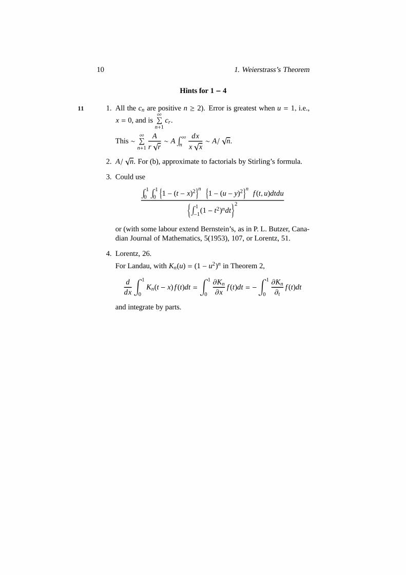
Hints for 1 − 4

1. All the cn are positiven ≥ 2). Error is greatest whenu = 1, i.e.,11

x = 0, and is∞∑

n+1cr .

This∼∞∑

n+1

A

r√

r∼ A

∫ ∞n

dx

x√

x∼ A/

√n.

2. A/√

n. For (b), approximate to factorials by Stirling’s formula.

3. Could use∫ 10

∫ 10

{

1− (t − x)2}n {

1− (u− y)2}n

f (t, u)dtdu{

∫ 1

−1(1− t2)ndt

}2

or (with some labour extend Bernstein’s, as in P. L. Butzer, Cana-dian Journal of Mathematics, 5(1953), 107, or Lorentz, 51.

4. Lorentz, 26.

For Landau, withKn(u) = (1− u2)n in Theorem 2,

ddx

∫ 1

0Kn(t − x) f (t)dt =

∫ 1

0

∂Kn

∂xf (t)dt = −

∫ 1

0

∂Kn

∂tf (t)dt

and integrate by parts.

Chapter 2

The Polynomial of BestApproximation ChebyshevPolynomials

4 The Lagrange Polynomial

We are givenn+ 1 values ofx, 12

x0, x1, . . . , xn

andn+ 1 constantsc0, c1, . . . , cn.Write

∏

(x) = (x− x0) · · · (x− xn).The polynomialp(x) of degree at mostn which takes the valuesci

at xi is, by the partial- fraction rule forp(x)/∏

(x),

∏

(x)n

∑

0

1x− xi

ci∏

(xi).

If the ci are the values atxi of a function f (x), we call p(x) theLagrange polynomial off (x) at thexi . Here we follow the usual termi-nology, although Waring (1779) used the polynomial before Lagrange(1795) and indeed it is clear that the formula was known to Newton.

Suppose that the valuesx0, . . . , xn are fixed. The following lemmasfollow from the definition of the Lagrange polynomial.

11

12 2. The Polynomial of Best Approximation...

Lemma 1. Given an aggregate of polynomials pα(x) of degree at mostn, whereα runs through an index-set I, such that

|pα(xi)| ≤ A, α in I ; i = 0, . . . , n.

Then, ifaα,r is the coefficient ofxr in pα(x),

|aα,r | ≤ AB,

whereB is independent ofα.

Proof. Write pα(xi) for ci . We have aB depending only on thexi . �

Lemma 2. (For brevity of expression, we translate de la Vallee Poussin,13

Leons, 74). If, at n+ 1 given points, two polynomials of degree at mostn take ’infinitely close’ values, their corresponding coefficients are in-finitely close.

Proof. Given ε, we have two polynomials saypα(x), qα(x) which dif-fer by at mostε for each of the valuesx0, . . . , xn. By Lemma 1, theircorresponding coefficients differ by at mostBε. �

5 Best Approximation

Let Pn be the set of polynomialsp(x) of degree less than or equal ton.Then

P0 ⊂ P1 ⊂ P2 · · ·

Define, for any particularp in Pn,

d(p, f ) = sup| f (x) − p(x)| f or a ≤ x ≤ b.

Let d = dn = dn( f ) = inf d(p, f ) for all p in Pn. Thend ≥ 0.Our first aim is to prove that there exists ap in Pn for which the inf. isattained, i.e., that, givenf (x) of C(a, b), there is apolynomial of degreen of best approximation.Later we shall prove uniqueness.

If f is given,d0 ≥ d1 ≥ d2 . . . ,

5. Best Approximation 13

and Theorem 1 asserts that limdn = 0.The existence of a polynomial of best approximation was known

to Chebyshev (or Tschebyscheff) (1821 - 1894) who was one of thefounders of the subject. The necessary proof was supplied byBorel(1905).

Theorem 4. There is a polynomial p(x) in Pn for which 14

sup| f (x) − p(x)| = d(= dn).

Proof. All our polynomials beingPn, we do not need the suffix n todenote degree, and the suffixes inp1, p2, . . . will be used to specify par-ticular polynomials ofPn. As here, we shall commonly omit the variablex form a polynomialp(x) or a function f (x). �

By definition ofd, there is a polynomialpm with

d ≤ d(pm, f ) < d +1m.

For all manda ≤ x ≤ b,

|pm(x)| ≤ d + 1+ sup| f (x)| = A.

By §4, Lemma 1, then + 1 coefficients of powersx0, x1, . . . , xn in thepm(x) all lie in a bounded region ofn + 1 space. This set of points inn + 1 space has at least one limit point, defining a polynomialp(x) forwhich

d( f , p) ≤ d( f , pm) + d(pm, p)

≤ d +1m+ ε

whereε → 0 asm → ∞ through a sub-sequence for which there isconvergence of the coefficients to their limits.

Therefored( f , p) = d.

Theorem 5. If f (x) is C(a, b) and p(x) satisfies Theorem 4 there aren+ 2 values (or more) at which

f (x) − p(x) = ±d,

with alternating sign.


Proof. g(x) = f (x)− p(x) is continuous. Divide (a, b) into sub-intervals 15

such thatg(x) does not take the value 0 in any (closed) sub-interval inwhich it takes the value±d. Denote byl1, l2, . . . , lm (numbered from leftto right) those of the sub-intervals in whichg(x) takes the value+d or−d. Defineε1, ε2, . . . , εm to be+1 or−1 according as the value is+d or−d. We have to prove that there are at least are at leastn+ 1 changes ofsign in the sequence ofε′s. Suppose there are fewer. We shall obtain acontradiction by constructing a polynomial of better approximation thanp(x). �

If all the ε′shave the same sign, say+, add a small constant top(x).This gives a polynomial of better approximation.

Generally, suppose that there arek changes of sign in the sequenceof ε′s, wherek ≤ n. Let εi , εi+1 be different. Thenl i and l i+1 cannotabut (sinceg(x) does not vanish in either), so we can choose a value ofx; lying between them. We have thusk values ofx; call them

x1, x2, . . . , xk.

Defineh(x) = ε1(x1− x)(x2− x) · · · (xk− x).h(x) has the same sign asg(x) in each of sub-intervalsl. We shall prove that, ifη is small enough,the polynomial ofPn

p(x) + ηh(x)

has better approximation tof (x) thanp(x) has.In those intervals of the original subdivision which are notl′s,

sup|g(x)| = d′ (say) < d.

Chooseη to make|ηh(x)| < d − d′(a ≤ x ≤ b), now,16

| f − p− ηh| = |g− ηh|.

In the l′s, this is less thand, sinceg, h have the same sign.And, in the sub-intervals other thanl′s,

|g− ηh| ≤ |g| + |ηh| < d′ + (d − d′) = d.

So p+ ηh approximates better tof thanp does.


Theorem 6. The polynomial p(x) of Theorem 4 is unique.

Proof. Suppose that two polynomialsp, q satisfy Theorem 4. Letr =12

(p+q). Then f −r = 12( f −p)+

12

( f −q). Thereforer satisfies Theorem

4, and so, by Theorem 5,f − r = ±d

for n+ 2 values ofx. �

But f − r = d only if f − p = f − q = d. Therefore there aren+ 2values ofx for which p(x) andq(x), polynomials of degree at mostn,are equal. Thereforep(x) ≡ q(x).

In future we can (by Theorem 6) describeas the best Pn that poly-nomial p(x) in Pn for which

sup| f (x) − p(x)| = d,

whered = inf d( f , q) for all q(x) in Pn. The numberd (or dn if it isnecessary to make thenn explicit) may be calledthe best approximation.

Theorem 7. Suppose f is C(a, b) and q is in Pn. Let there be n+ 2values of x at which f− q takes values alternating in sign

d1,−d2, d3, . . . , (−1)n+1dn+2.

Then the best approximation d satisfies 17

d ≥ mindi

Proof. Suppose thatd < di(i = 1, . . . , n + 2) and letp be the bestPn.Thenp− q = ( f − q)− ( f − p) takes alternate signs at then+ 2 values inthe hypothesis. Thereforep− q (which is inPn) has at leastn+ 1 zeros.This is a contradiction. �

Corollary. Let q be in Pn and let

sup| f − q| = d′.

Suppose thatf − q takes the values±d′ alternately forn+ 2 valuesof x. Thend′ = d andq is the bestPn.

Proof. By theorem 6,d ≥ d′. But d ≤ d′, sinced is the best approxima-tion. �


6 Chebyshev polynomials

Theorem 4 guarantees the existence of the bestPn for a given f . It isonly in special cases that the explicit calculation of this polynomial ispracticable. Theorem 7 and its corollary can often be turnedto use.Easy exercises:

For x2 in (0, 1), the bestP0 is12

, the bestP1 is x+18

.

For x4 in (−1, 1), the bestP3 is x2+

18

.

Consider now the general problem.

A. Among all pn(x) with coefficient ofxn equal to 1, find that which de-viates least from 0 in (−1, 1) in other words, that for whichsup|pn(x)| = d is least.

This problem can be stated in the equivalent form.

B. Find the best approximation inPn−1 to xn in (−1, 1).

From Theorem 7 (Corollary) we wish to find apn(x) which takes the18

values±d alternately atn+1 points (why notn+2 points?). Enlightenedguessing soon leads to the answer

pn(x) = dcosnθ wherex = cosθ.

It is worth while to give Chebyshev’s own proof of this, whichdoesnot depend on guesswork.

Theorem 8. Among all pn(x) with coefficient of xn equal to1, the poly-nomial

2−n+1 cosnθ where x= cosθ

deviates least from0 in (−1, 1).

Proof. let p(x) = xn+· · · be the required polynomial, andd = sup|p(x)|.

�

By Theorem 5, there aren+1 values ofx (at least) wherep(x) = ±d.These may be end-points or interior points of (−1, 1). At such a point

6. Chebyshev polynomials 17

which is an interior point,p(x) has a maximum or minimum and sop′(x) = 0. Sincep′(x) has degreen− 1, then+ 1 values must be 1,−1andn− 1 others, sayx1, x2, . . . , xn−1.

The two polynomials of degree 2n

d2 − p2 and (1− x2)p′2

have the same zeros, namely, 1,−1 and each ofx1, x2, . . . , xn−1 doubly.Comparing the coefficients ofx2n we have

n2(d2 − p2) = (1− x2)p′2.

Solving this differential equation forp we find, puttingx = cosθ,

p = dcos(nθ +C)

Sincep(x) is a polynomial,C = 0. But

cosnθ = 2n−1 cosn θ + lower powers of cosθ,

and so = 2−n+1.

The polynomials revealed by Theorem 8 are named after Chebyshev 19

and (following the alternative spelling of his name) we define

Tn(x) = cos(n arc cosx).

The early members of the sequence are

T0(x) = 1, T1(x) = x T2(x) = 2x2 − 1

T3(x) = 4x3 − 3x, T4(x) = 8x4 − 8x2+ 1.

Their mode of definition is restricted to (−1, 1) and it is in that inter-val that their utility mainly lies. But many of their properties hold for allvalues ofx. Some useful results are collected in Theorem 9; the proofscan easily be supplied.

Theorem 9. (1) y= Tn(x) satisfies the differential equation

(1− x2)y′′ − xy′ + n2y = 0.


(2) Tn(x) is the coefficient of tn in the expansion of the generating func-tion

1− tx

1− 2tx+ t2

(3) the recurrence relation

Tn(x) = 2xTn−1(x) − Tn−2(x) (n ≥ 2).

(4) an explicit formula for the coefficients

Tn(x) =∑

(−1)kn

n− k

(

n− kn

)

2n−2k−1xn−2k

summed for0 ≤ k ≤[n2

]

(5) orthogonality with the weight-function1/√

(1− x2)

∫ 1

−1

Tn(x)Tm(x)√

(1− x2)dx=

0(m, n)12π(m= n)

(6) for |x| > 1,

2Tn(x) = {x+√

(x2 − 1)}n + {x+√

(x2 − 1)}n.

Note

The calculation of polynomials of best approximation is in practice20

troublesome. See de la Vallee Poussin, ChapterVI. For a method of cal-culation by a convergent sequence, see Polya, Comptes Rendus (Paris)157 (1913), 840.

Chapter 3

Approximations to |x|

7

We now take up the central problem of polynomial approximation, 21

namelyGiven a function f (x), how high is the degree of the polynomial

necessary to approach it with an assigned accuracy?The answer may well depend on structural properties off (x). For

instance, we may guess (rightly) that we can predict a lower degree iff (x) is assumed to be differentiable instead of only continuous. Thebest theorems on these matter lie fairly deep. We shall go through someheuristic motion of finding from particular cases what truthappears tobe and then deciding how to try to establish it.

A useful function to study with care is|x| in (−1, 1). This functionwas the basis of Lebesgue’s proof of Theorem 1.

From Exercises 1, 2 at the end of ChapterI , the deviation from|x|of a polynomial of degreen of any of the three types used in provingTheorem 1 is of order 1/

√n.

Let us clarify our mode of speech. If, for somep(x) in Pn,

| f (x) − p(x)| = 0{ϕ(n)}

we will say that the approximation is 0{ϕ(n)}. If, moreover, there is nop(x) in Pn for which

| f (x) − p(x)| = 0{ϕ(n)}

19

20 3. Approximations to|x|

we will say that the approximation isactually0{ϕ(n)}.Study of the proofs of Theorem 1 might lead us to conjecture that

the best approximation inpn to |x| is actually 0(1/√

n).We proceed to show that, in fact, it is actually 0(1/n). This will be22

proved, following Bernstein, Lecons Ch.I, by elementary (though ratherlengthy) algebra.

To approximation to|x| in (−1, 1) is the same thing as to approximateto x in (0, 1) by polynomials whose exponents are all even, and this iswhat we shall do.

If d2n is the best approximation tox in (0, 1) by

a0 + a1x2+ · · · + anx2n

we shall prove that

12n+ 1

> d2n >1

4(1+√

2)· 1

2n− 1.

Bernstein went further and proved thatd2n ∼ C/n, whereC is aconstant which he evaluated as 0.282± 0.004.

The theorems of this Chapter will not be used later in the course,and any one who wishes may note above inequalities ford2n and passon to Chapter IV.

8 Oscillating polynomials

Definition. If 0 ≤ α0 < α1 · · · < αn andAi , 0 (all i), we say that

p(x) = A0xα0 + A1xα1 + · · · + Anxαn

is anoscillating polynomialin (0, 1) if sup|p(x)| is attained forn + 1values ofx in 0 ≤ x ≤ 1. We shall suppose theα′s integers.Illustrations.

(1) αi = 2i + 1 T2n+1(x) satisfies

(2) αi = i T2n(√

x).

8. Oscillating polynomials 21

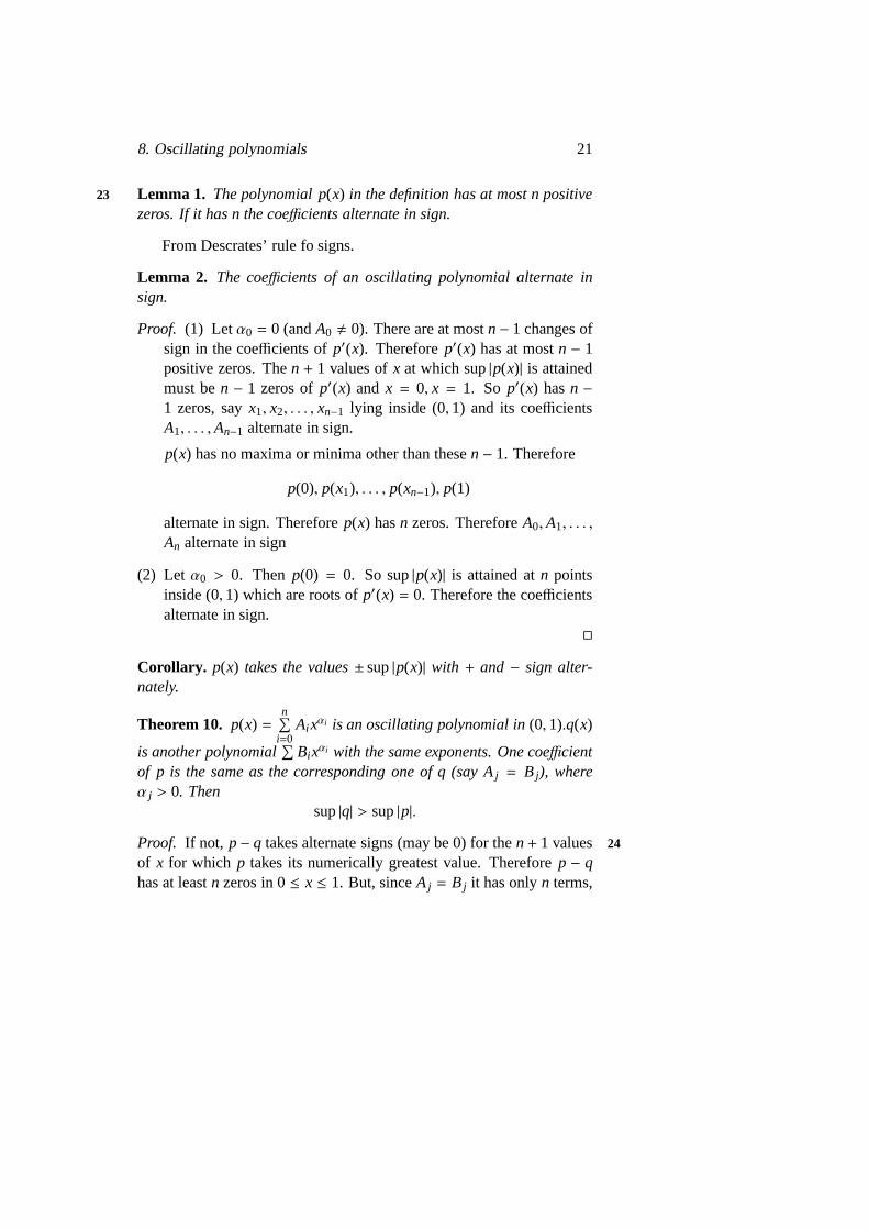
Lemma 1. The polynomial p(x) in the definition has at most n positive23

zeros. If it has n the coefficients alternate in sign.

From Descrates’ rule fo signs.

Lemma 2. The coefficients of an oscillating polynomial alternate insign.

Proof. (1) Letα0 = 0 (andA0 , 0). There are at mostn− 1 changes ofsign in the coefficients ofp′(x). Thereforep′(x) has at mostn − 1positive zeros. Then + 1 values ofx at which sup|p(x)| is attainedmust ben − 1 zeros ofp′(x) and x = 0, x = 1. So p′(x) hasn −1 zeros, sayx1, x2, . . . , xn−1 lying inside (0, 1) and its coefficientsA1, . . . ,An−1 alternate in sign.

p(x) has no maxima or minima other than thesen− 1. Therefore

p(0), p(x1), . . . , p(xn−1), p(1)

alternate in sign. Thereforep(x) hasn zeros. ThereforeA0,A1, . . . ,

An alternate in sign

(2) Let α0 > 0. Thenp(0) = 0. So sup|p(x)| is attained atn pointsinside (0, 1) which are roots ofp′(x) = 0. Therefore the coefficientsalternate in sign.

�

Corollary. p(x) takes the values± sup|p(x)| with + and − sign alter-nately.

Theorem 10. p(x) =n∑

i=0Ai xαi is an oscillating polynomial in(0, 1).q(x)

is another polynomial∑

Bi xαi with the same exponents. One coefficientof p is the same as the corresponding one of q (say Aj = B j), whereα j > 0. Then

sup|q| > sup|p|.

Proof. If not, p− q takes alternate signs (may be 0) for then+ 1 values 24

of x for which p takes its numerically greatest value. Thereforep − qhas at leastn zeros in 0≤ x ≤ 1. But, sinceA j = B j it has onlyn terms,


and so at mostn−1 changes of sign in its coefficients and so (by Lemma1) at mostn− 1 positive zeros. This is a contradiction. �

Converse of Theorem 10. p(x) andq(x) are two polynomials with thesame exponents and one coefficient the same (A j = B j, whereα j > 0).If

sup|p| < sup|q|

for every suchq, thenp is an oscillating polynomial.

Proof. We gives the gist of the proof, without setting out all the detailin full. It uses a ’deformation’ argument like that of theorem 5. �

Suppose thatp(x) is not an oscillating polynomial. Thenp(x) takesthe values±M, whereM = sup|p(x)|, at h points, sayxk(k = 1, . . . , h),whereh < n + 1. We can construct a polynomialr(x) =

∑

Ci xαi withC j = 0 andr(xk) = p(xk). (Then + 1 coefficientsCi have to satisfy atmostn+ 1 equations; the determinant can be proved, 0).

We can takeε and intervals round thexk, outside which|p(x)| <M − ε and inside each of whichp(x) andr(x) have the same sign.

Chooseλ to makeλ|r(x)| < ε for 0 ≤ x ≤ 1.

Then sup|p− λr | < sup|p|.

But p− λr satisfies the conditions for aq, giving a contradiction.Apply theorem 10, takingp(x) to be a constant multiple of one of25

the oscillating polynomialsT2n(√

x) andT2n+1(x). We obtain

Corollary 1. If q(x) = a0 + a1x+ · · · anxn and M= sup|q(x)| in (0, 1),then

|ai | ≤ M|ti |(i = 0, 1, . . . , n),

where ti is the coefficient of xi in T2n(√

x).26

Corollary 2. If q(x) = a0x + a1x3+ · · · anx2n+1 and M = sup|q(x)| in

(0, 1), then|ai | ≤ M|ti |(i = 0, . . . , n)

where ti is the coefficient of x2i+1 in T2n+1(x).

8. Oscillating polynomials 23

Theorem 11. To a given set of exponents there corresponds an oscillat-ing polynomial in(0, 1), which is unique except for a constant factor.

Proof. Let α0, α1, . . . , αn be the given exponents in ascending order.Suppose that the coefficient of xαk is given to beK. �

We need to prove that among all the polynomials with the givenexponents

q(x) = B0xα0 + · · · + Bk−1xαk−1 + kxαk + · · · + Bnxαn,

there is a uniqueq(x) for which sup0≤x≤1

|q(x)| attains its lower bound.

Clearly sup|q(x)| is a continuous function of then variables (B0 · · · ,Bk−1, Bk+1, . . . , Bn). Its lower bound is greater than 0 by Corollary 1 ofTheorem 10. It is less than or equal toK, as is seen by taking theB′s tobe small. Again by Corollary 1, we need only consider values of Bi forwhich

|Bi | ≤ K|ti | (i = 0, 1, . . . , k− 1, k+ 1, . . . , n),

whereti is the coefficient of xαi in T2αn(√

x).TheBi lie in a bounded closed region ofn space, and so they have at

least one set of values for which sup|q(x)| attains its lower bound. Thisproves the existence of an oscillating polynomial. Uniqueness followsfrom Theorem 10.

Theorem 12. If

p(x) = xα0 + A1xα1β1+ · · · + Anxαn

βn

and q(x) = xα0 + B1xβ1 + · · · + Bnxβn

are both oscillating polynomials in(0, 1) where

0 < α0 < β1 < α1 < β2 < · · · < βn < αn,

then sup|p(x)| > sup|q(x)|.


Proof. By Lemma 2, the coefficients fo ofp(x) alternate in sign and sodo those ofq(x).

q(x) − p(x) = B1xβ1 − A1xα1 + B2xβ2 − · · · − Axαnn

hasn variation of sign, and so the equation

q(x) − p(x) = 0

has at mostn positive roots. �

Suppose the theorem false and

sup|p(x)| ≤ sup|q(x)|.

Thenq(x) − p(x) has the sign ofq(x) (it may be 0) for the valuesxn(k = 1, . . . , n+ 1) at which|q(x)| takes its maximum value. Thereforeq(x) − p(x) vanishes forn valuesξ1, . . . , ξn such that

xi ≤ ξ1 ≤ x2 ≤ ξ2 ≤ · · · ≤ ξn ≤ xn+1.

Moreover, there aren+ 1x′s and onlynξ′s so at least onex, sayxi27

must satisfyξi−1 < xi < ξi (giving meaning toξ0, ξn+1).We shall now compute the sign ofq(xi) by two different methods

and obtain contradictory results.Firstly, in (0, ξ1), q(x)− p(x) has the sign of its dominant termB1xβ1,

which is negative. By following the changes of sign along thesequence,q(x) − p(x) has sign (−1)i in (ξi−1, ξi). At xi , q(x) − p(x) and alsoq(x)have the sign (−1)i .

Secondly, for small values ofx, q(x) had the sign of its first term,which is positive. Thereforeq(x1) > 0. Soq(x2) < 0, and generally,q(xi) has the sign (−1)i+1.

This is a contradiction.The same arguments can be used to prove

Theorem 12 (Extension).If

p(x) = A0xα0 + · · · + Ai−1xαi−1 + xm+ Ai+1xαi+1 + · · · + Anxαn

9. Approximation to|x| 25

q(x) = B0xβ0 + · · · + Bi−1xβi−1 + xm+ Bi+1xβi+1 + · · · + Bnxβn

are both oscillating polynomials in(0, 1), where

0 ≤ α0 < β0 < · · · < αi−1 < βi−1 < m< βi+1 < αi+1 · · · < βn < αn,

thensup|p(x)| > sup|q(x)|.

9 Approximation to |x|

Theorem 13. If

p(x) = x+ a1x2+ a2x4

+ · · · + anx2n

is an oscillating polynomial in(0, 1), then

12n+ 1

> sup|p(x)| > 1

2(1+√

2)(2n− 1)(n > 1).

Note. If n = 1, the second inequality is to be replaced by equality. The28

oscillating polynomial isx−(

12+

1√

2

)

x2.

Proof. Taken > 1. By Theorem 12, sup|p(x)| is less than the supremumof the oscillating polynomial

x+ b1x3+ · · ·

with exponents 1, 3, 5, . . . 2n+ 1. But that polynomial is (−1)nT2n+1(x)/(2n+ 1). This gives the first inequality of the theorem. �

By Theorems 12 and 10, the oscillating polynomialx+ b1x3+ · · ·+

bn−1x2n−1 has smaller maximum modulus than the polynomialx+c2x4+

· · · + cr x2n with exponents 1, 4, 6, . . . , 2n. But the former polynomial is(−1)n−1T2n−1(x)/(2n− 1), with maximum modules 1/(2n− 1). We shallnow construct a polynomial of the latter form (with no term inx2).

With the notation of the hypothesis forp(x), write sup|p(x)| = m.


Then, ifµ > 0,

∣

∣

∣

∣

∣

x1+ µ

+ a1

(

x1+ µ

)2

· · · + an

(

x1+ µ

)2n ∣

∣

∣

∣

∣

≤ m.

Therefore

|x(1+ µ) + a1x2+ a′2x4

+ · · · + a′nx2n| ≤ m(1+ µ)2

i.e., |p(x) + µ(x+ c2x4+ · · · + cnx2n)| ≤ m(1+ µ)2.

Therefore

|µ(x+ c2x4+ · · · + cnx2n)| ≤ m

{

(1+ µ)2+ 1

}

and so |x+ c2x4+ · · · + cnx2n| ≤ m

{

(1+ µ)2+ 1

}

/µ

This is true for all positive values ofµ, and so we can replace the29

right-hand side by its minimum, which is 2m(1+√

2).As we said, the maximum modulus of a polynomial with exponents

1, 4, 6, . . . , 2n is greater than 1/(2n− 1) and therefore

m>1

2(1+√

2).

12n− 1

We have now all the material for the final result announced at theend of §7.

Theorem 14. If d2n is the best approximation to x in(0, 1) by

a0 + a1x2+ · · · + anx2n,

then1

2n+ 1> d2n >

1

4(1+√

2)· 1

2n− 1.

Proof. d2n is the maximum modulus of the oscillating polynomial

A0 + x+ A1x2+ A2x4

+ · · · + Anx2n.

Let p(x) andmhave the same meanings as in Theorem 13. �

9. Approximation to|x| 27

By Theorem 10, d2n < m.Write q(x) − A0 = x+ A1x2

+ · · · + Anx2n.So, by Theorem 10,

sup|q(x) − A0|

is greater than the maximum modulus ofp(x), the oscillating polynomialwith exponents 1, 2, 4, . . . , 2n and coefficient of x equal to 1; that is tosay, is greater thanm.

But sup|q(x) − A0| ≤ d2n + |A0| ≤ 2d2n.Therefore 2d2n > m.The inequalities of Theorem 13 form give the started inequalities

for d2n.

Notes

1. Example. Find the polynomial inPn for which the coefficient of xk 30

is 1 and which deviates least from 0.

2. The definition on page 22 of an oscillating polynomial can be ex-tended to a system

A0ϕ0 + · · · + Anϕn(x),

if the ϕ′s satisfy certain conditions. See Bernstein, Lecons, 1 or As-chieser, 67

Hint

1. If k, n are both even or both odd, considerTn(x), otherwiseT2n(√

x).

Chapter 4

Trigonometric Polynomials

10 Trigonometric polynomials. Modulus of Conti-nuity

The central problem of approximation, namely the degree of the poly- 31

nomial required an assigned closeness to a given function, yields moreeasily to trigonometric than to algebraic treatment. Trigonometric seriesand in particular Fourier series have been in the fore-frontof Analysisfor something like a century, and knowledge about them has been avail-able for any problem of approximation.

A trigonometric polynomials is

t(x) =12

a0 + (a1 cosx+ b1 sinx)+ · · ·+ (an cosnx+ bn sinnx). This

can be writtentn(x) if an , 0 orbn , 0 and we wish to display theorderof the polynomial. We can denote byTn the set of all polynomials whichare sums of multiples of coskx and sinkx for <≤ k ≤ n. (There will beno confusion with the Chebyshev polynomialsTn(x) of §6).

The functiont(x) is periodic with period 2π (and, in general, with nosmaller period). We say thatf (x) is C(2π) if it is continuous with period2π.

The problem of approximating to aC(2π) function by a trigono-metric polynomial is essentially the same as that of approximating toa C(a, b) function by an algebraic polynomials. In the first place, theanalogue of Theorem 1 holds.

29

30 4. Trigonometric Polynomials

Theorem 15(Weierstrass). If f (x) is C(2π) then, givenε, there is t(x)such that

| f (x) − t(x)| < ε (all x)

This will emerge as a by-product of theorem 18, and we shall givean independent proof here. You should, however, read Notes1− 3 at theend of this chapter.

In statements about periodic functions, values ofx differing by mul-32

tiple of 2π will be regarded as the same.

Lemma 1. The equation tn(x) = 0 has at most2n roots.

(Prove by expressing in term of tan12

x or of expix).

Corollary 1. Two t′ns which take the same values at2n + 1 points areidentical.

Corollary 2. If two t′ns have2n common zeros one is a consult multipleof the order

The reader should verify that there is an analogue of the Lagrangepolynomial of §4, namely

The polynomial inTn which takes the valuesci at xi(i = 0, 1, . . . , 2n)is

P(x)∑ 1

2 sin x−xi2

ci

P′(xi)

where P(x) =∏

sinx− xi

2.

We shall take for granted the trigonometric analogues of Theorem4 − 7 (pages 14− 17) about best approximation. Briefly, for a givenf (x) in C(2π), there is uniquet(x) of best approximation inTn whichis characterized byf (x) − t(x) taking its greatest numerical value, withalternating sign, for alt least 2n+ 2 values ofx. Proofs can be found inthe book of de la Vallee Poussin or Natanson.

10. Trigonometric polynomials. Modulus of Continuity 31

Illustrations:

1) If f (x) = tn−1(x) + (an cosnx+ bn sinnx). thentn−1(x) gives thebest approximation inTn−1 to f (x).

Proof. f− tn−1 takes the values±√

(a2n + b2

n) alternately at 2n points.�

2) An interesting example is Weiertrass’s non-differentiable function 33

f (x) =∞∑

r=0

ar cosbr x

where 0< a < 1, b is an odd integer andab> 1. We shall prove thatthe best approximation inTn to f (x) is

t(x) =k

∑

r=0

ar cosbr x, wherebk ≤ n < bk+1.

Proof. f(x) − t(x) =∑∞

k+1 ar cosbr x. �

This takes its greatest value∞∑

k+1ar at x = 0. Cosbk+1x takes the

values±1 alternately at integral multiples ofπ/bk+1, of which there are2bk+1 in a period.

Sinceb is an odd integer, cosbr x for r > k+ 1 takes the same valuesat those points as cosbk+1x.

Now 2bk+1 ≥ 2n+ 2 and sof (x)− t(x) takes its numerically greatestvalue for at least 2n+ 2 values ofx.

Corollary. The approximation given by this t(x) is A/nα, whereα =log(1/a)/ logb.

Proof. The approximation is

ak+1

1− a=

b−α(k+1)

1− a∼

11− a

·1nα

�


Modulus of continuity.Let f (x) beC(a, b) and define

ω(δ) = sup| f (x2) − f (x1)| for |x2 − x1| ≤ δ.

Thenω(δ) is continuous, increases asδ increases, and tends to 0 asδ tends to 0. We shall find that the rapidity with whichω(1/n) tends to0 asn→ ∞ gives the clue to the approximation tof (x) attainable inPn

or Tn.If f (x) isC(2π), the same definition ofω(δ) holds. Observe that now34

the greatest value ofω(δ) isω(π)Properties ofω(δ) are collected in the following theorem.

Theorem 16. (1) If n is an integer,

ω(nδ) ≤ nω(δ).

(2) If k > 0, ω(kδ) ≤ (k + 1)ω(δ).

(3) If ω(δ) = for someδ > 0, then f(x) is a constant.

Proof. (1) f (x+ nh) − f (x) =n−1∑

k=o

{

f (x+ kh+ h) − f (x+ kh)}

.

Forh ≤ δ, the R.H.S. is numerically at mostnω(δ).

(2) If k is not an integer, letn be the integer next greater. Then

ω(kδ) ≤ ω(nδ) ≤ nω(δ) ≤ (k + 1)ω(δ).

(3) f (x) is constant in any interval less thatδ, and so everywhere.�

Lipschitz condition. Def. f(x) satisfies the Lipschitz condition oforderα(briefly, is Lip. α) in a given interval, if for everyx1, x2 in it,

| f (x2) − f (x1)| ≤ A|x2 − x1|α.

It follows thatω(δ) ≤ Aδα.In this, 0 < α ≤ 1. If α > 1, f (x) can only be a constant,be a

constant, because then

ω(δ) ≤ nω(δ/n) ≤ Aδα/nα−1.

Making n→ ∞, we haveω(δ) = 0.

11. Fourier and Fejer Sums 33

11 Fourier and Fejer Sums

We collect for reference in Theorem 17 some well-known facts. Proofs 35

can be found in any text-book of analysis which includes a chapter onFourier Series.

Theorem 17. (1) The sum

Sn =12

a0 +

n∑

r=1

(ar cosrx + br sinrx)

for the Fourier Series of f(x) is equal to

1π

∫ π

0{ f (x+ t) + f (x− t)}

sin(

n+ 12

)

t

2 sin 12t

dt.

(2) | f (x) − Sn(x)| < M(A logn+ B), where M= sup| f (x)| and A, B areconstants.

(3) If σn = (S0 + S1 · · · + Sn−1)/n

is the Fejer(C1) sum of the Fourier series of f(x), then

σn =1nπ

∫ π

0f (x+ 2t)

(

sinntsint

)2

dt.

(4)1

sin2 t=

∑∞−∞

1

(t + kπ)2(t , kπ).

The result (2), which cannot be improved, shows that, in general,the Fourier series of a function gives a poor approximation in the sensemeasured by sup| f (x) − Sn(x)|. As the R.H.S. of (2) tends to infinitywith n, (2) does not include Weierstrass’s Theorem 15. The sense inwhich the Fourier series does give the best approximation isthe mean-square sense (omitted here). It is known that the Fejer sumsσn of (3)behave more regularly than the Fourier sumsSn; this is due to the kernel(sinnt/ sint)2 in the integral forσn being positive, whereas the kernel inSn takes both signs. The next theorem gives the approximation to f (x)afforded by (σn (x).


Theorem 18. If f (x) has modulus of continuityω(δ), then 36

| f (x) − σn(x)| ≤ Aω(1/n)|logω(1/n)|.

Proof. We first putσn(x) into a form more convenient than that of The-orem 17(3). Sincef is periodic

∫ π

0f (x+ 2t)

sin2 nt

(t + kπ)2dt =

∫ (k+1)π

kπf (x+ 2t)

sin2 nt

(t2)dt.

�

Then, from (3) and (4) of Theorem 17,

σn =1nπ

∫ π

0f (x+ 2t)

sin2 nt

sin2 tdt =

1nπ

∫ ∞

−∞f (x+ 2t)

sin2 nt

t2dt,

and so, by changing the variable fromt to t/n,

σn =1π

∫ ∞

−∞f (x+

2tn

)sin2 t

t2dt

σn − f =1π

∫ ∞

−∞

{

f (x+2tn

) − f (x)

}

sin2 t

t2dt.

Therefore

| f − σn| ≤2π

∫ ∞

0ω(2t/n)

sin2 t

t2dt.

The integral on the R.H.S. is the sum of the integrals over (0, 1),(1,X) and (X,∞). This gives

| f − σn| ≤2π

{

ω(2/n) +∫ X

1ω(2t/n)

dt

t2+ ω(π)

∫ ∞

X

dt

t2

}

≤2π

{

ω(2/n) + ω(2/n)∫ X

1

t + 1

t2dt +

ω(π)X

}

≤ 2π

{

ω(2/n)(2+ log X) +ω(π)

X

}

.

ChooseX = 1/ω(2/n) and we have a result equivalent to that stated.


Corollary 1. Theorem 1537

Corollary 2. If ω(δ) < Aδα(0 < α < 1), then | f − σn| < ABnα , where

B = B(α) is independent of f .

Proof.

| f − σn| ≤2π

∫ ∞

0ω(2t/n)

sin2 t

t2dt

≤2α+1Aπnα

∫ ∞

0tα

sin2 t

t2dt

The estimates in Chapter III would lead us to suspect that, ifwe canfind at(x) which approximates tof (x) more closely thanσn(x) does, wemay get rid of the logω(1/n) on the R.H.S. of Theorem 18. It is easy tosee how to try to do this. The logarithm arises from integrating a termin 1/t. The Fejer sum is

Fr(x, n) =1Jr

∫ ∞

−∞f

(

x+2tn

) (

sintt

)

2r dt

for r = 1 andJr = π. If r ≥ 2, there will be no term in 1/t. We shallachieve our purpose by takingr = 2. �

Lemma 1. (1) J2 =

∞∫

−∞(

sintt

)4dt = 2π

3 .

(2) F2(x, n) is in T2n−1.

Proof. (1)

J2 =

π∫

0

sin4 t∞∑

−∞

1(t + kπ)4

dt

=16

π∫

0

sin4 td2

dt2

(

1

sin2 t

)

dt

=16

π∫

0

sin4 t

(

6

sin4 t− 4

sin2 t

)

dt =2π3.


(2) Reversing the steps by whichF1(x, n) was obtained in the first partof the proof of Theorem 18. we have

F2(x, n) =32π

36n

π∫

0

f (x+ 2t) sin4 ntd2

dt2

(

1

sin2 t

)

dt.

Then sin4 ntd2

dt2

(

1

sin2 t

)

= sin4 nt

(

6

sin4 t− 4

sin2 t

)

. �38

Nowsinntsint

is the sum of multiples of coskt wherek ≤ n− 1. Hence

sin4 ntd2

dt2

(

1

sin2 t

)

is the sum of multiples of coskt wherek ≤ 4n − 2.

Moreover, the expression is even and has periodπ, sok takes only evenvalues, 21 say, where 1≤ 2n− 1. Finally,

∫ π

0f (x+ 2n) cos 21tdt =

12

∫ 2π

0f (u) cosl(u− x)du

andF2(x, n) is in T2n−1.

Theorem 19. | f (x) − F2(x, n)| ≤ 3ω(1/n).

Proof. F2(x, n) − f (x) =32π

∞∫

−∞

{

f (x+2tn

) − f (x)}

(

sintt

)4

dt. �

Now | f (x+2tn

) − f (x)| ≤ ω(

2|t|n

)

≤ (2|t| + 1)ω(1/n) from Theorem

16 (2). Therefore

| f (x) − F2(x, n)| ≤ ω(1/n)3π

∫ ∞

0(2t + 1)

(

sintt

)4

dt = Aω(1/n),

whereA = 1+6π

∫ ∞0

sin4 t

t3dt. But

∫ ∞

0

sin4 t

t3dt

∫ ∞

0|sin3 t

t2|dt =

12

∫ π

0

sin3 t

sin2 tdt = 1

(again by use of Theorem 17(4)).

So A < 1+6π< 3.


Theorem 20. If f (x) is C(2π) and f′(x) is continuous with modulus ofcontinuityω1(δ), then

| f (x) − F2(x, n)| ≤Anω1(1/n) where A< 5/2.

Proof. F2(x, n) − f (x) =32π

∞∫

0

{

f

(

x+2tn

)

+ f

(

x− 2tn

)

− 2 f (x)

} (

sintt

)4

dt.

The modulus of the term within{ } is 39

|2n

∫ t

0

{

f ′(

x+2un

)

− f ′(

x− 2un

)}

du|

≤2n

t∫

0

ω1

(

4un

)

du

≤ 2nω1

(

1n

)

t∫

0

(4u+ 1)du

=2nω1

(

1n

)

(2t2 + t)

�

Therefore

| f (x) − F2(x, n)| ≤Anω1

(

1n

)

,

where

A =3π

∞∫

0

(2t2 + t)

(

sintt

)4

dt =3π

sin2 tdt+3π

∞∫

0

sin4 tt3

dt <3π

(

π

2+ 1

)

<52

Theorem 20 can be extended to higher derivatives. Iff (x) has anr-th derivative with modulus of continuityωr (δ), the approximation at-tainable inTn is a constant multiple ofn−rωr(1/n).

Notes on Chapter IV 40


1. Use the singular integral (de la Vallee Poussin)

1Jn

π∫

−π

cos2n 12

(t − x) f (t)dt,

whereJn is the value of the integral whenf (t) = 1, to give a directproof of Theorem 15.

2. Assuming Theorem 15 proved, deduce Theorem 1 from it.

3. Deduce Theorem 15 from Theorem 1 as follows:

(a) Prove that, iff (x) is C(0, π), it can be approximated uniformlyby at(x) containing cosines only.

(b) By applying (a) to the even functions

2g(x) = f (x) + f (−x)

2h(x) ={

f (x) − f (−x)}

sinx,

deduce thatf (x) is uniformly approximately by at(x).

4. With the notation of Illustration (2), Corollary, page 31, prove thatWeierstrass’s function

∑

ar cosbr x satisfies a Lipschitz condition oforderα.

Hints41

1 Follow Theorem 2. Detail is in Natanson, 10.

2 Approximate to coskxand sinkxby a finite number of terms of theirexpansions in powers ofx.

3 (a) Puty = cosx.

(b) g(x), h(x) are uniformly approximately in (−π, π). So is g(x)sin2 x + h(x) sin2 x. So is f (x) cos2 x, and hencef (x)(sin2 x +cos2 x).


4 Givenh, choosen so thatbnh ≤ 1 < bn+1h.

f (x+ h) − f (x− h) = −2∞∑

1

ar sinbrhsinbr x

=

n∑

1

+

∞∑

n+1∣

∣

∣

∣

∣

∞∑

n+1

∣

∣

∣

∣

∣

≤ 2∞∑

n+1

ar=

2an+1

1− a∣

∣

∣

∣

∣

n∑

1

∣

∣

∣

∣

∣

≤ 2hn

∑

1

arbr= 2abh

anbn − 1ab− 1

<2ban+1

ab− 1

But an+1= b−α(n+1) < hα.

Hence | f (x+ h) − f (x− h)| < Ahα.With more trouble (Aschieser and Krein, 167) this can be proved

best possible.

Chapter 5

Inequalities, etc.

12 Bernstein’s and Markoff’s Inequalities

Theorem 21(Bernstein). If t(x) =12

ao +∑n

1(ak coskx+ bk sinkx) then 42

|t′(x)| ≤ nsup|t(x)|.

Proof. Suppose, on the contrary, that

sup|t′(x)| = nl,

where l > sup|t(x)|. �

t′(x), being continuous, attains its bounds and so, for somec, t′(a) =±nl and we will suppose that

t′(c) = nl.

Sincenl is a maximum value oft′(x),

t′′(c) = 0.

Define S(x) = l sinn(x− c) − t(x).

Thenr(x) = S′(x) = nl cosn(x− c) − t′(x).

S(x) and r(x) both have ordern.Consider the points

uo = c+ π/2n, uk = uo + kπ/n(1 ≤ k ≤ 2n).

41

42 5. Inequalities, etc.

Then

S(uo) = 1− t(uo) > 0

S(u1) = 1− t(u1) < 0

· · · · · ·S(u2n) = 1− t(u2n) > 0

Each of the 2n intervals (uo, u1), (u1, u2), . . . , (u2n−1, u2n) then contains azero ofS(x).say

S(yi ) = 0,

whereui < yi < ui+1, (0 ≤ i ≤ 2n− 1). Clearly43

y2n−1 < yo + 2π.

Write y2n = yo + 2π.

Then S(y2n) = S(yo) = 0.

By Rolle’s Theorem, there is a zeroxi of r(x) inside each interval(yi , yi+1) where 0≤ i ≤ 2n− 1. Clearly

x2n−1 < xo + 2π.

Now r(c) = nl − t′(c) = 0.Since the polynomialr(x) of ordern has at most 2n zeros, it follows

that, for somek,c ≡ xk (mod 2π).

But r′(c) = −t′′(c) = 0.Thereforec(and soxk) is a double zero (at least) ofr(x).Therefore thexi(0 ≤ i ≤ 2n − 1) provide at least 2n + 1 zeros of

r(x). This is only possible ifr(x) ≡ 0, and soS(x) is a constant. ButS(uo) > 0 andS(u1) < 0 and we have a contradiction

Corollary 1. t(x) = sinnx shows that the result is the best possible.

Corollary 2. The algebraic equivalent is- If p(x) has degree n and|p(x)| ≤ M in (−1, 1), then

|p′(x)| ≤ nM√

(1− x2).

12. Bernstein’s and Markoff’s Inequalities 43

Proof. Put

t(θ) = p(cosθ)

t′(θ) = −p′(cosθ) sin(θ).

The bound for|p′(x)| given in Corollary 2 fails at the end-points±1. A 44

better result, due to Markoff, is

|p′(x)| ≤ Mn2,

as will be proved in Theorem 22. �

Lemma 1. Let

xk = cos(2k − 1)π

2n(k = 1, 2, . . . , n)

be the zeros of the Chebyschev polynomial Tn(x). If q(x) is in Pn−1, then

q(x) =1n

n∑

k=1

(−1)k−1√

(1− x2k)q(xk) ·

Tn(x)x− xk

.

Proof. Both sides are inPn−1 and so it is sufficient to show that theyagree for then valuesxk. As x→ xk,

Tn(x)x− xk

→ T′n(xk) =n

√

(1− x2k)

sin(n arc cosxk)

=n(−1)k−1

√

(1− x2k)

Also, for x = xk, every term on the R.H.S. except the k-th vanishes.�

Lemma 2. Suppose that q(x) is in Pn−1 and |q(x)| ≤ 1√

(1− x2)(−1 <

x < 1).

Then|q(x)| ≤ n (−1 ≤ x ≤ 1).


Proof. With the notation of Lemma 1, if−x1 = xn ≤ x ≤ x1,

√

(1− x2) ≥√

(1− x21) = sin

π

2n≥ 1

n.

Therefore Lemma 2 is true forxn ≤ x ≤ x1. If x1 < x ≤ 1 (or−1 ≤ x < xn) Lemma 1 gives

|q(x)| ≤1n|∑ Tn(x)

x− xk|,

since all thex− xk are positive (or all negative). Now45

Tn(x) = 2n−1∏

(x− xk),

and soT′n(x)Tn(x)

=

∑ 1x− xk

.

�

Therefore |q(x)| ≤ 1n|T′n(x)|.

But, if x = cosθ,T′n(x) =nsinnθ

sinθ, which gives

|T′n(x)| ≤ n2.

Theorem 22(Markoff). If p(x) is in Pn, then

|p′(x)| ≤ n2 sup|p(x)| − 1 ≤ x ≤ 1.

Proof. If sup|p(x)| = M, take in Lemma 2,

q(x) =p′(x)Mn.

�

Corollary. p(x) = Tn(x) shows that the result is the best possible.

13. Structural Properties Depend on the... 45

13 Structural Properties Depend on the closeness ofthe approximation

Theorem 21 can be used to prove theorems of a type converse to The-orems 18-20. Theorem 23, which is complementary to Theorem 18,Corollary 2, will suffice to show the method.

Theorem 23. Let f(x) be C(2π). Suppose that, for all n, the best ap-proximation in Tn to f(x) is less than A/nα, where0 < α < 1. Then f(x)is Lip.α.

Proof. Let tn(x) satisfy

| f (x) − tn(x)| ≤Anα.

Define u0(x) = t1(x)

an(x)t2n(x) − t2n−1(x) (n ≥ 1).

�

Then f (x) is the sum of the uniformly convergent series∞∑

0un(x). 46

Chooseδ with 0 < δ ≤12

, andmsuch that

2m−1 ≤ 1δ< 2m.

Suppose|x− y| ≤ δ. We have

| f (x) − f (y)| ≤m−1∑

0

|un(x) − un(y)| +∞∑

m

|un(x)| +∞∑

m

|un(y)|.

We shall find upper bounds for the terms on the R.H.S.

|un(x)| ≤ |t2n(x) − f (x)| + | f (x) − t2n−1(x)|

≤A

2nα +A

2(n−1)α=

A(1+ 2α)2nα .


Therefore∞∑

m

|un(x)| ≤ A(1+ 2α)∞∑

m

12nα =

A(1+ 2α)1− 2−α

12mα .

This gives

| f (x) − f (y)| ≤m−1∑

o

|un(x) − un(y)| +B

2mα .

Theorem 21 applied toun(x) gives

|u′n(x)| ≤ 2n sup|un(x)| ≤ A(1+ 2α)2n(1−α).

By the mean-value theorem,

|un(x) − un(y)| ≤ |u′n(ξ)||x− y| ≤ A(1+ 2α)2n(1−α)δ

Therefore

| f (x) − f (y)| ≤ A(1+ 2α)δm−1∑

o

2n(1−α)+

B2mα .

PuttingC = A(1+ 2α) and using1

2m < δ, we have

ω(δ) ≤ Cδm−1∑

o

2n(1−α)+ Bδα.

If now α < 1,47

m−1∑

o

2n(1−α)=

2m(1−α) − 1

21−α − 1<

2m(1−α)

21−α − 1.

Use now 2m ≤ 2δ

and we find

ω(δ) <

(

21−α

21−α − 1C + B

)

δα

See Notes 1-4 at the end of the Chapter.

14. Divergence of the Lagrange Sequence 47

14 Divergence of the Lagrange Sequence

There is a sense in which the Lagrange polynomial of degreen (§4) fit-ted to a functionf (x) at n+ 1 points equally spaced through an intervalfollows the function closely. It is natural to expect that, by increasingn,the approximation would improve and we might, for instance,find an-other proof of Theorem 1 on these lines. Such expectations are falsified.Unless heavy restrictions are laid onf (x), the sequence of Lagrangepolynomials diverges except for certain special values ofx.

We shall construct an example of this phenomenon.

Lemma. Let p(x) be the Lagrange polynomial which takes the value0at the2m values of x

k/m (−m≤ k ≤ m; k , 2)

and takes the value1/m when x= 2/m. Then, if m is odd,|p(

12

)

| → ∞as m→ ∞.

Proof. The polynomialp(x), of degree 2m, is

1m

(x+ 1)(x+ m−1m ) . . . x(x− 1/m)(x− 3/m) . . . (x− 1)

(2/m+ 1)(2/m+ m−1m ) . . . 2/m(2/m− 1/m)(2/m− 3/m) . . . (2/m− 1)

This gives for|p(

12

)

| 48

1m

3m(3m− 2) . . .m(m− 2)(m− 6) . . . 1.1.3. . . .m

22m(m+ 1)(m+ 1) . . . 2.1.1.2 . . . (m− 2)

�

This can be estimated by forming it into factorials and usingStirb-ing’s theorem. More simply, we can prove that it tends to∞ by groupingthe factors as follows:

|p(

12

)

| =m− 1

2(m+ 1)(m+ 2)(m− 4)A2BC,


where A =3.54. . .m

2.4 . . . (m− 1)

B =(m+ 2)(m+ 4) . . . (2m+ 1)

(m+ 1)(m+ 3) . . . 2m

C =

(

−2m+ 3m+ 1

) (

3m+ 5m+ 3

)

. . .

(

3m2m− 2

)

.

HereA > 1, B > 1, and the factors ofC decrease from left to right,the last being greater than 3/2. SoC > (3/2)m−1.

Note.x =12

has been taken for ease of calculation. The conclusion holds

for other values ofx.

Theorem 24 (Borel). There is f(x) in C(−1, 1) whose nth Lagrangepolynomial does not converge to f(x) as n→∞.

Proof. Define a continuous curveCk which coincides with Ox outsidethe interval (3−k−1, 3−k) and has maximum 3−k−1 at the midpoint of thatinterval. For example we can defineCk by

y = 3−k−1 sin{

(3k+1x− 1)π/2}

.

�

We shall use theCk to construct a curveS.Pk,S(x) will denote theLagrange polynomial which takes the same values asS for the valuesx = 1/3k, where−3k ≤ 1 (integer)≤ 3k.

We shall constructS so thatPk,S

(

12

)

does not converge to the point49

onS wherex =12

. Observe first thatPk,Ck−1 is the Lagrange polynomial

in the Lemma withm= 3k. From the Lemma, given A, there ish1 suchthat

|Pk,Ck−1

(

12

)

| > 2A if k− 1 > h1.

There are two possibilities:

(a) With h1 fixed, Pk,Ch1

(

12

)

does not tend to 0 ask→ ∞. ThenS can

be taken to beCh1; or

14. Divergence of the Lagrange Sequence 49

(b) there existsr such that

|Pk,Ch1

(

12

)

| < 12

A for all k > r1.

Chooseh2 > max(h1, r1).DefineD2,k to be the sine-curves inCh1 andCk−1(k − 1 ≥ h2), and,

for the rest, the x-axis in (−1, 1).

D2,k is a continuous curve; its ordinate forx =12

is 0, and

Pk,D2,k = Pk,Ch1+ Pk,Ck−1.

From above, sincek− 1 ≥ h2,

|Pk,D2,k

(

12

)

| > 2A− 12

A.

Again, there are two possibilities:

(a) With h2 fixed,Pk,D2,k

(

12

)

does not tend to 0 ask → ∞. ThenS can

be taken to beD2,h2; or

(b) there existsr2 such that

|Pk,D2,kh2

(

12

)

| < 14· A for all k > r2.

Chooseh3 > max(h2, r2). 50

DefineD3,k to be the sine-curves inCh1,Ch2 andCk−1(k − 1 ≥ h3)and, for the rest, the -axis in (−1, 1). After n repetitions, there are twopossibilities:

(a) There is aDn,hn for which thek th Lagrange polynomial does not

tend to 0 atx =12

; and this serves forS; or

(b) there is an infinite sequenceDn,hn for which

|Phn+1,Dn,hn

(

12

)

| > 2A− 12

A− 14

A− . . . − A

2n−1> A.


As n → ∞,Dn,hn defines a continuous curveS whose ordinate for

x =12

is 0. Its Lagrange polynomial takes values greater thanA for

x =12

when its degree ish1, h2, . . . , hn, . . ..

Notes51

1. Weierstrass’s function∑

ar cosbr x illustrates Theorem 18 (Corol-lary 2) and Theorem 23. See Chapter IV, note 4.

2. If α = 1, the best that can be proved in Theorem 23 is thatω(δ) <Aδ log(1/δ). The latter part of the argument can be adapted forthis purpose (Natanson, 91).

The function∑∞

1sinnx

n2 satisfiesdn <1n

, but is not in Lip.1 (Natan-

son, 93).

3. A condition which is necessary and sufficient ofdn < A/n is that

| f (x+ h) − 2 f (x) + f (x− h)| < Bh.

(Zymund, Duke Mathematical Journal, 12(1945)47 or Natanson,96).

4. (Extension of Theorem 23). If, forf (x), dn < A/np+α (p =integer, 0 < α < 1), then f (x) has a pth derivativef (p)(x) in Lipα.

5. For further ‘negative results’ like Theorem 24, see Natanson, 369– 388. For example, the Lagrange polynomial taking the values of|x| atn equally spaced points in (−1, 1) converges to|x| asn→ ∞for no value ofx expect 0,±1.

Chapter 6

Approximation in Terms ofDifferences

15

This is the only chapter in the course, of which the results are not clas- 52

sical. The point of view here might lead to a re-orientation towardsalgebraic rather than trigonometric polynomials.

In Theorem 20 (and its known extensions) the approximation attain-able inPn or Tn to a differentiable functionf (x) is expressed in terms ofits first higher derivative. We shall now give simple examples which leadus to suppose that bounds ofdifferencesof f (x) rather than derivativesmay be more directly related to the closeness of the approximation.

Example 1.If f (x) attains its greatest value atx2 and its least atx1, thenthe best approximation inP0 is

12{ f (x1) + f (x2)}

and do =12{ f (x2) − f (x1)} = 1

2sup|∆ f |

This depends solely on the first difference off (x); the derivative off (x)- if it exists-has no bearing on it.

Now raise the degree by one.

51

52 6. Approximation in Terms of Differences

Example 2.If f (x) is C(0, 1), there is a linear functionp(x) for which

| f (x) − p(x)| ≤ sup| f (x+ 2h) − 2 f (x+ h) + f (x)|,

the sup being taken over allx, h such that

0 ≤ x ≤ x+ 2h ≤ 1.

Proof. Definep(x) to be equal tof (x) at x = 0 andx = 1 Write53

g(x) = f (x) − p(x).

�

Then|g(x)| attains its maximum,M, for 0 ≤ x ≤ 1 atx1, say.

If 0 ≤ x1 ≤12

, takex = 0, h = x1. Then

|g(x+ 2h) − 2g(x+ h) + g(x)| = |g(2x1) − 2g(x1) + g(0)| ≥ M.

If12< x1 ≤ 1 takex = 2x1 − 1, h = 1− x1. Then

|g(x+ 2h) − 2g(x+ h) + g(x)| = |g(1)− 2g(x1) + g(1− x1)| ≥ M.

But the second difference ofg(x) and f (x) are equal.By a longer argument it is possible to prove the corresponding result

for P2 and the third difference.The general result was conjectured in 1949 by H. Burkill.

Theorem 25. There is a number Kn depending only on n such that givenf (x) in C(a, b), there is a polynomial p(x) in Pn−1 for which

| f (x) − p(x)| ≤ Kn sup|∆n( f )|

(where the supremum is taken for all sets of n+ 1 points x, . . . , x+ nh in(a, b))

16. Definition and Properties of thenth Difference 53

The theorem looks innocent, but attempts at it failed until Whitneyit in 1955. He took for hisp(x) the Lagrange polynomial for the pointsof division of (a, b) into n − 1 equal parts. His work does not yield anestimate ofKn for generaln; in view of Theorem 24, we should hardlyexpect good value ofKn.

Whitney’s elegant arguments are too long for reproduction here, and54

the reader is referred to his paper in journal de Mathematiques 36(1957),67-95.

It is worth observing, however, that instead of the usualnth differ-ence with equal increments, we can take a more generalnth differencedepending of the values off (x) at n+ 1 arbitrary points. The difficultythen disappears and the polynomial of best approximation can be usedinstead of the Lagrange polynomial.

16 Definition and Properties of thenth Difference

Ifϕ(u) = (u− ho)(u− h1) · · · (u− hn),

thenth divided difference off (x) for the values specified is commonlydefined by

Dn = Dn( f ; ho, . . . , hn) =n

∑

i=0

f (hi )ϕ′(hi)

.

In what follows it will be convenient to suppose that

ho > h1 > · · · > hn

To define annth difference∆n, as distinct from a divided difference,we naturally take

∆n = HnDn,

whereHn is homogeneous of degreen in theh′s.The most suitable definition ofHn appears to be

Hn = 2n/Tn,


where Tn = Tn(ho, h1, . . . , hn) =n

∑

i=0

|ϕ′(hi)|−1.

In the special case of equal increments withho − hn = nh, this gives55

Hn = n!hn, which is right.As a further check on the appropriateness of ourHn, we observe that

if a function is numerically less thanA, its nth difference∆n is numeri-cally less than 2nA.

In working with Dn,∆n, etc., we shall specify the function and thevalues of the variables only so far as is necessary for clarity.

We are now in a position to restate and prove Theorem 25, taking∆n( f ) to be the differenceHnDn( f ) just defined.

Theorem 25′. Theorem 25 is true with Kn = 2−n and∆n( f ) as just de-fined and the supremum taken over all values of ho, . . . , hn in (a, b).

Proof. Given f (x), takep(x) to be its polynomial of best approximationof degree at mostn − 1. Then f (x) − p(x) takes its greatest numericalvalue atn+ 1 points, with signs alternately+ and−. Thesen+ 1 pointswe takes asho, . . . , hn. �

Since thenth difference of a polynomial of degreen−1 is 0, we have

∆n( f ; ho, . . . , hn) = Hn

n∑

i=o

f (hi ) − p(hi)ϕ′(hi)

So |∆n| = Hnd

∑

|ϕ′(hi)|−1= 2nd,

by definition ofHn.Therefore, for allx in (−1, 1),

| f (x) − p(x)| ≤ d ≤ 2−n sup|∆n( f )|.

This proves Theorem 25′.Alternatively we can prove Theorem 25′, starting from the upper56

bound of|∆n| instead of from the polynomial of best approximation.

16. Definition and Properties of thenth Difference 55

Suppose, then, that sup|∆n| = L and that the boundL is assumedfor the valuesho, h1, . . . , hn of the independent variable. Define points(hi , yi) for i = 0, 1, . . . , by taking

yi = f (hi) − (−1)kL2n ,

wherek is i or i+1 according as∆n( f , ho, . . . , hn) is positive or negative.Constructa p(x) of Pn−1 through then points (hi , yi) for i = 0, 1, . . . ,

n− 1. Writeg(x) = f (x) − p(x).

Since∆n(p) ≡ 0, |∆n(g)| = |∆n( f )| attains its upper bound forh0, h1,. . . , hn. From the definition of∆n, the value ofg(hn) which makes|∆n(g, h0, h1, . . . , hn)| = L is (−1)kL/2n, wherek is n or n + 1 accord-ing as∆n( f , ho, . . . , hn) is positive or negative.

We prove that|g(x)| ≤ 2−nL for all x. Suppose that|g| takes valuesgreater thanL/2n, sayg(h′i ) > L/2n for a valueh′i betweenhi−1 andhi+1

whereg(hi ) = 2−nL. Then, from the definition ofTn,

Dn(g, ho, . . . , hi−1, h′i , hi+1, . . . , hn)

> 2−nLTn(ho, . . . , hi−1, h′i , hi+1, . . . , hn)

and so, by definition of∆n,

∆n(g, ho, . . . , hi−1, h′i , hi+1, . . . , hn) > L,

which is a contradiction. We have therefore

| f (x) − p(x)| = |g(x)| ≤ 2−n sup|∆n( f )|,

which is Theorem 25′. 57

For the next result let us call then+ 1 values

−1,− cosπ

n, . . . , cos

π

n, 1

at which the Chebyshev polynomial cos(n arc cosx) assumes the values±1 the Chebyshev points of the interval (−1, 1).


Theorem 26. Suppose that1 ≥> ho > h1 ≥ · · · ≥ hn ≥ −1. Then

Tn(ho, . . . , hn) ≥ 2n−1

and the sign= holds if and only if the hi are the Chebyshev points.

Proof. The polynomialqn(x) of degreen which takes the value (−1)i athi(i = 0, . . . , n) is

qn(x) = ϕ(x)n

∑

i=0

(−1)i

ϕ′(hi) (x− hi ).

�

Thenqn(x) = anxn+ · · · + ao, where

an =

n∑

i=o

1|ϕ′(hi)|

= Tn(ho, . . . , hn).

Write tn(x) = 2−n+1an cos(n arc cosx).Thenqn(x) − tn(x) has degreen− 1 at most.If an < 2n−1, then|tn(x)| < 1 andqn(x) − tn(x) has the sign ofqn(x)

for the n + 1 valuesho, . . . , h1. If an = 2n−1 the same is true on theunderstanding thatqn(x) − tn(x) may vanish for any of these values. Sothe polynomialqn(x) − tn(x), of degree at mostn− 1, hasn zeros. Thisis a contradiction ifan < 2n−1, and is only possible foran = 2n−1 whenqn(x) ≡ tn(x). This proves the theorem.

Corollary. For 1 ≥ ho ≥ · · · ≥ hn ≥ −1,Hn ≤ 2.

Bibliography

[1] Achieser,N.I.- (English by Hyman), Theory of Approximation, 58

New Yor, 1956.

[2] Bertstein,S.- Lecons sur les properties extremales et la meilleureapproximation des fucntions analytiquesd′une variables reelle,paris, 1926

[3] Jackson,D.- The theory of approximation, (Ameriacan Mathemat-ical Society Colloquium,XI New York, 1930.

[4] Natanson,I,P. - (German by Bogel), Konstruktive Funktionentheo-rie, Berlin, 1955.

[5] de la Vallee Poussin, G.J.- Lecons sur 1’ approximation ses func-tions dune variable reelle, Paris, 1919.

57

APPENDIXApproximation byPolynomials in the ComplexDomain

1 Runge’s Theorem

The problem considered till now was the approximation of a given con- 59

tinuous function on a finite closed interval by polynomials in a real vari-able. Even for functions of two variables, we considered only the prob-lem of approximation by polynomials in two independent realvariablesx, y. in what follows, we shall consider the approximation of a functionin a domain in the plane (open connected set) by polynomials in thecomplex variablez= x+ iy (which are analytic functions of the variablez).

Let pn(z) be a sequence of polynomials and suppose thatG (whichwe assume is not empty) is the largest open set in whichpn(z) converges,uniformly on every compact subset. (This is the type of approximationwe shall consider; the problem of approximation on closed sets moredifficult). By Weierstrass’s theorem the limit of the sequencepn(z) is ananalytic function inG. There is moreover, a purely topological restric-tion onG, viz., every connected componentD of G is simply connected:for, if C is a sample closed curve contained inD andB is its interior, then

59

60 BIBLIOGRAPHY

(maximum modulus principle)

supz∈B∪C

|pn(z) − pm(z)| = supz∈C|pn(z) − pm(z)| → as 0n,m→ ∞

so that the sequencepn(z) converges uniformly onB∪C. HenceB∪C ⊂G and sinceD is a connected component andC ⊂ D, B ⊂ D.

The main theorem, which is the analogue of Weierstrass’s approx-60

imation theorem (Th.1, p.2) and which includes a converse of the re-marks made above, runs as follows.

Theorem A (Runge).Let D be a domain in the plane and f an analyticfunction in D. Then f can be approximated, uniformly on everycompactsubset of D, by rational functions whose poles lie outside D.If D issimply connected, f may be approximated by polynomials.

We begin by funding a sequence of open regionsGn, n = 1, 2, 3, . . .bounded by polygons such thatGn is relatively compact inGn+1, whoselimit is D. We may takeGn as a subsequence of the sequenceBm, where

Bm is defined to be the interior of the union of those squaresk

2m ≤

x ≤k+ 12m ,

12m ≤ y ≤

l + 12m , k, 1 integers,|k|, |l| ≤ 22m

, which lie in D.

The boundary ofGn can be split into a finite number of simple closedpolygonsCn,k can be joined by a simple are which does not meetGn toa point on the boundary ofD. If Cn =

⋃

kCn,k is the boundary ofGn we

have

f (z) =1

2πi

∫

Cn

f (t)t − z

dt, z ∈ Gn.

By the definition of the integral, we may approximatef (z) uniformlyin Gn−1 by finite sums of the form

fn(z) =1

2πi

∑ f (tr )tr − z

(tr+1 − tr )

wheretr are certain points onCn. Hence ifεn ↓ 0, we can find a se-quence of rational functionsRn such thatRn has poles at most onCn

and

(1) | f (z) − Rn(z)| < εn in Gn−1.

1. Runge’s Theorem 61

The main idea in the proof of the theorem is contained in the next 61

step, which we state as a separate lemma.

Lemma. Let C be a simple are joining the points zo and z1 and K acompact set not meeting C. Then, any rational function whoseonlypossible pole is at zo can be approximated, uniformly on K, by rationalfunctions which no poles expect possibly at z1.

Proof of the lemma. Let ε > 0 be given and 2d be the distancebetweenC andK. We find pointsao, . . . , aµ onC, ao = zo, aµ = z1 suchthat |ak+1 − ak| ≤ d. Let R(z) be the given rational function. There aretwo polynomialsp andq so that

R(z) = p(z) + q

(

1z− zo

)

and we have only to approximateq

(

1z− zo

)

= f (z). Since f (z) is ana-

lytic in |z−a1| > d and is finite at∞, the Laurent expansion off (z) abouta1 contains no positive powers ofz− a1 and converges uniformly on ev-ery compact subset of|z− a1| > d. A suitable partial sum then gives us

a polynomialp1 with∣

∣

∣

∣

∣

f (z) − p1

(

1z− a1

)∣

∣

∣

∣

∣

<ε

µ + 1for z ∈ K. Repeating

this process, we find successively, polynomialsp j , j = 1, . . . , µ with∣

∣

∣

∣

∣

p j

(

1z− a j

)

− p j+1

(

1z− a j+1

)∣

∣

∣

∣

∣

<ε

µ + 1for z ∈ K.

Then clearly∣

∣

∣

∣

∣

f (z) − pµ

(

1z− aµ

)∣

∣

∣

∣

∣

< ε, z ∈ K

and the lemma follows.

Proof of Theorem.Let D be any domain andf analytic inD. Let Gn

be the sequence of regions exhaustingD described above. There is a62

rational functionrn with poles at most onCn+1 such that∣

∣

∣

∣

∣

f (z) − rn(z)∣

∣

∣

∣

∣

<12n

onGn.

62 BIBLIOGRAPHY

Every point of the boundary ofGn+1 can be joined be an arc notmeetingGn to the boundary ofD, so that, by the lemma, there is a

rational functionRn with poles outsideD such that∣

∣

∣

∣

∣

Rn(z) − rn(z)∣

∣

∣

∣

∣

<12n

on Gn and | f (z) − Rn(z)| < 1n

on Gn. The first part of Runge’s theorem

is proved. IfD is simply connected, then every connected componentof the complement is unbounded (unlessD is the whole plane in whichcase the theorem is trivial). Hence every point of the boundary of Gn+1

can be joined to a pointz1(|z1| ≥ 2r) by an arc which does not meetGn,r being such thatGn is contained in the circle|z| < r.

Now it follows as above that there is a rational functionRn(z) withall its poles lying in|z| ≥ 2r, with

∣

∣

∣

∣

∣

f (z) − Rn(z)∣

∣

∣

∣

∣

<12n

onGn.

If we expandRn(z) in a Taylor series aboutz = 0 (which convergesuniformly for |z| ≤ r), then a suitable partial sumpn(z) satisfies

∣

∣

∣

∣

∣

Rn(z) − pn(z)∣

∣

∣

∣

∣

<12n

onGn

so that∣

∣

∣

∣

∣

f (z) − pn(z)∣

∣

∣

∣

∣

<1n

onGn.

This complete the proof of Runge’s theoremThe same argument proves the following theorem

THEOREM A 1. Let D be any plane domain. From each connectedcomponent of the complement of D, choose a point zα. Then any analyticfunction in D can be approximated uniformly on every compactset in D63

by rational functions which have poles at most at the points zα.

Runge’s theorem is of importance in the theory of functions.Asan instance of its applicability we prove the following extension to anarbitrary of Mittag-Leffler’s theorem

THEOREM. Let D be a plane domain and aν, ν = 1, 2, . . . sequence ofpoints in D having no limit point in D. Let pνbe polynomials (without

2. Interpolation 63

constant term). Then there is a meromorphic function f in D with poles

at most at the aν such that f(z) − pν

(

1z− aν

)

is analytic at aν.

Proof. We can construct a sequenceGn, n = 1, 2, . . . of regions so thatGn is relatively compact inGn+1,

⋃

n Gn = D and so that any point of theboundary ofGn can be joined to a point not inD by an arc not meetingGn. Let

fn(z) =∑

aν∈Gn

pν

(

1z− aν

)

the sum being over those (finitely many)aν which lie inGn. Sincefn+2−fn+1 is analytic inGn+1, we can find a rational functionRn+1 with nopoles inD such that

∣

∣

∣

∣

∣

fn+2(z) − fn+1(z) − Rn+1(z)∣

∣

∣

∣

∣

<12n for z in Gn.

�

Since the poles of theRn+1 lie outsideD and the series

∞∑

n=no+1

( fn+1 − fn − Rn)

converges uniformly inGno, it follows easily that we may take 64

f (z) = f2(z) +∞∑

n=2

( fn+1(z) − fn(z) − Rn(z)).

2 Interpolation

For functionsf of a real variable, ifpn is the (Lagrange) polynomialpof degreen which agrees withf at n + 1 equally spaces points on aninterval, the sequencepn in general diverges asn→ ∞. The behaviourfor functions of a complex variable is more satisfactory. Weproceed toprove two of the main theorems.

64 BIBLIOGRAPHY

Let C be a simple closed rectifiable curve andf (z) a function an-alytic inside and onC. Let t1, . . . , tn+1 be n + 1 points insideC (notnecessarily distinct). Then the polynomialpn(z) of degreen such thatpn(ti) = f (ti ), i = 1, . . . , n + 1 (multiplicity being taken into account ifsome of theti coincide) is easily seen to be given by

f (z) − pn(z) =1

2πi

∫

C

(z− t1) · · · (z− tn+1)(t − t1) · · · (t − tn+1)

f (t)t − z

dt.

Our first theorem is as follows. It is also due to Runge.

THEOREM B. Let f(z) be analytic for|z| < R,R > 1 and pn(z) thepolynomial of degree n with pn(zi ) = f (zi), i = 0, 1, . . . , n, where the ziare the(n+ 1)th roots of unity.

Thenpn(z) → f (z) as n→∞

uniformly for |z| ≤ < R.

Proof. Let C be the circle|z| = ρ′, ρ′ > ρ, ρ > 1. Then, for|z| ≤ ρ,65

f (z) − pn(z) =1

2πi

∫

c

zn+1 − 1tn+1 − 1

f (t)t − z

dt,

so that

| f (z) − pn(z)| = 12π|∫

c

zn+1 − 1tn+1 − 1

f (t)t − z

dt|

≤ 1+ ρn+1

(ρ′n+1 − 1)(ρ′ − ρ)M (M = sup

z∈C| f (z)|)

→ 0 asn→ ∞ sinceρ′ > ρ, ρ′ > 1.

�

The next theorem is due to Fejer and is considerably deeper; it con-tains TheoremB.

Let C be a simple closed curve and suppose thatw(z) maps the exte-rior of C one-one conformally onto|w| > 1 in such a way that the points

2. Interpolation 65

at infinity correspond. Then, as is well known,w(z) is one-one continu-ous onC. Letα(n)

i , i = 0, 1, . . . , n be then+ 1 points ofC correspondingto the (n+ 1)th roots of unity in the w-plane. Then we have

THEOREM C. Let f(z) be a function analytic inside and on Cand pn(z)the polynomial of degree n which equals f(z) at the pointsα(c)

i . Thenpn(z)→ f (z), uniformly inside and on C.

We begin with a lemma.

Lemma.

limn→∞

n∏

i=0

∣

∣

∣

∣

z− α(n)i

∣

∣

∣

∣

1(n+1)= A|w(z)|.

uniformly on any compact set exterior to C,A > 0 being a constant 66

(depending on C).

Proof of the lemma. Let z = z(w) be the inverse ofw = w(z) and letwo, . . . ,wn be the (n+ 1)th roots of unity. We prove first that

1. limn→∞

n∏

i=0

∣

∣

∣

∣

∣

z(w)−z(wi )w−wi

∣

∣

∣

∣

∣

1(n+1)= A.

The logarithm of the term on the left is

2. limn→∞

1n+1

∑ni=o log

∣

∣

∣

∣

∣

z(w)−z(wi )w−wi

∣

∣

∣

∣

∣

=12π

2π∫

olog

∣

∣

∣

∣

∣

z(w)−z(eiθ)w−eiθ

∣

∣

∣

∣

∣

dθ

and the limit is uniform forw in a compact set in|w| > 1.

Nowz(w) − z(ζ)

w− ζis an analytic function ofζ for |ζ | > 1 and fixedw,

includingζ = ∞, ζ = w. Hence the integral in (2) is equal to

limζ→∞

log∣

∣

∣

∣

∣

z(w) − z(ζ)w− ζ

∣

∣

∣

∣

∣

= log A, say

(we have only to make the substitutionζ → 1/ζ and use the Poisonintegral).

From (1), it follows that

limn→∞

n∏

i=o

|z(w) − z(wi)|1

(n+1)

|w− wi |1/(n+1)= lim

n→∞

n∏

i=0|z(w) − z(wi)|

1(n+1)

|wn+1 − 1|1/(n+1)

66 BIBLIOGRAPHY

=

limn→∞

n∏

i=0|z(w) − z(wi)

1(n+1)

|w|= A

and the lemma follows on substitutingw = w(z).

Proof of Theorem.Let CR(R > 1) denote the image underz(w) of the67

circle |w| = R; we can chooseR> 1 such thatf is analytic inside and onCR. Let 1< r1 < r2 < R; and put

πn(z) =n

∏

i=o

(z− α(n)i ).

We have

f (z) − pn(z) =1

2πi

∫

Cr2

πn(z)πn(t)

f (t)t − z

dt.

If z is onCr1 andt onCr2,

limn→∞

∣

∣

∣

∣

∣

πn(z)πn(t)

∣

∣

∣

∣

∣

1n+1

=r1

r2(by the lemma)

so that limn→∞

[

supz∈Cr1

| f (z) − pn(z)|]

1n+1≤ r1

r2< 1.

Consequentlyf (z) − pn(z)→ o uniformly for zonCr1.The theorem follows at once from the maximal modulus principle.

3 Best Approximation

In this section we shall consider the problem of best approximation.Let K be a compact set containing infinitely many points andf (z) a68

continuousfunction onK. Our aim is to prove the existence and unique-ness of a polynomialpn(z) of degreen such that

d( f , pn) = supz∈K

∣

∣

∣

∣

∣

f (z) − pn(z)∣

∣

∣

∣

∣


is least. in general, of course, this minimumd( f , pn) does not tend tozero asn→ ∞.Existence of a polynomial of best approximation.

Let Pn be the family of all polynomials of degree≤ n, and let f (z)be a continuous function on the compact setK. Let

d( f ) = d = infp∈Pn

d( f , p) = infp∈Pn

(supz∈K| f (z) − p(z)|).

Then we have the

THEOREM D. There exists a p∈ Pn with d( f , p) = d.

Proof. Any polynomial p ∈ Pn takes values 0 or 1 atn points at most.HencePn is a quasi-normal family of ordern, (theorem of Montel, see[1] p. 67) i.e., given a sequencepν of polynomials inPn, there is asubsequencepνk andn pointszi such thatpνk converges, uniformly onevery compact set not containing thezi , either to a finite limit functionor to∞. In the first case it is clear thatpνk converges uniformly on anycompact set (which may contain some of thezi). �

There is a sequencep(ν) of polynomials ofPn so thatd( f , p(ν))→ d.Then, clearly, ifz ∈ K, |p(ν)(z)| ≤ d + 1+ sup

ζ∈K| f (ζ)| for largeν (we may 69

suppose that holds for allν). Let p(νk) be a subsequence converging out-siden pointszi , uniformly on compact sets. SinceK contains infinitelymany points there are points ofK not equal to anyzi , and it these pointsz, |p(νk)(z)| is bounded. Hence the limit outsidezi is finite and conse-quently,p(νk) converges uniformly on any compact set. From Cauchy’sinequality, it follows then that the corresponding co-efficients of p(νk)

converge, so that limk→∞

p(νk)(z) = p(z) ∈ Pn. Then we have

d ≤ d( f , p) ≤ d( f , p(νk)) + d(p(νk), p)→ d

so thatd( f , p) = d.[If K contains a circle|z− a| < r, r > o, the existence of a sequence

p(νk) converging uniformly on any compact set follows at once, as in thecase (Ch.II ,Th.4, p.14) if we use the Cauchy inequalities.]

68 BIBLIOGRAPHY

Uniqueness of the polynomial of best approximation.We shall deduce the uniqueness fro the following theorem, asin the

case of a real variable.Let p ∈ Pn satisfy d( f , p) = d( f ). Then | f (z) − p(z)| attains its

maximum at atleastn+ 2 distinct points ofK.(The proof is similar in principle to the proof ofTh.5, p.14).

Proof. Suppose thatf (z)−p(z) = g(z) attains its maximum modulus atmpoints (m≤ n+ 1)z1, . . . , zm of K. Then, we can construct a polynomialq(z) of degreen such thatq(zi ) = g(zi ). Givenε > o, we can findδ > 070

so that if

|ζ1 − ζ2| < δ, |g(ζ1) − g(ζ2)| < ε, |q(ζ1) − q(ζ2)| < ε

�

Let K1 be the set obtained fromK by removing the points of the(open) discs|z− zi | < δ. Then

supz∈K1|g(z)| = d1 < d = sup

z∈K|g(z)|.

Let 1 > η > o be sufficiently small. Considerg(z) − ηq(z); then for|z− zi | < δ, |g(z) − g(zi)| < ε, |ηq(z) − ηq(zi )| < ηε, so that|g(z) − ηq(z)| =|η(g(zi ) − g(z)) + ηg(z) − g(z) + η(q(z) − q(zi ))| (sinceq(zi ) = g(zi )) <ηε + ηε + (1− η)d < d if 2ε < d

If we chooseη so small that

supz∈K1|g(z) − ηq(z)| < d

we have supz∈K|g(z) − ηq(z)| < d

andd( f , p+ ηq) < d, contradicting the definition ofd.

THEOREM E. The polynomial of degree≤ n of best approximation isunique.

Proof. Let d( f , p) = d = d( f , q); let r(z) =12

(p(z) + q(z)). �

Bibliography

[1] Montel, P. : Lecons sur les familles normales de fonctions analy-tiques et leurs applications, Gauthiers-Villars, Paris, 1927

[2] Walsh,J.L. : Approximation by polynomials in the complex do-main, Mem. des Sciences Mathem., Paris, 1935

[3] Walsh, J.L. : Interpolation and approximation by rational func-tions in the complex domain, Amer. Math. Soc. Colloquium Pub-lications,Vol.XX, 1935.

71

lectures on approximation by polynomials - …publ/ln/tifr16.pdflectures on approximation by...

Documents