lectures on classical mechanics

Lectures onClassical Mechanics

John C. BaezDerek K. Wise

(version of September 7, 2019)

i

c©2017 John C. Baez & Derek K. Wise

iii

Preface

These are notes for a mathematics graduate course on classical mechanics at U.C. River-side. I’ve taught this course three times recently. Twice I focused on the Hamiltonianapproach. In 2005 I started with the Lagrangian approach, with a heavy emphasis onaction principles, and derived the Hamiltonian approach from that. This approach seemsmore coherent.

Derek Wise took beautiful handwritten notes on the 2005 course, which can be foundon my website:

http://math.ucr.edu/home/baez/classical/

Later, Blair Smith from Louisiana State University miraculously appeared and volun-teered to turn the notes into LATEX . While not yet the book I’d eventually like to write,the result may already be helpful for people interested in the mathematics of classicalmechanics.

The chapters in this LATEX version are in the same order as the weekly lectures, butI’ve merged weeks together, and sometimes split them over chapter, to obtain a moretextbook feel to these notes. For reference, the weekly lectures are outlined here.

Week 1: (Mar. 28, 30, Apr. 1)—The Lagrangian approach to classical mechanics:deriving F = ma from the requirement that the particle’s path be a critical point ofthe action. The prehistory of the Lagrangian approach: D’Alembert’s “principle of leastenergy” in statics, Fermat’s “principle of least time” in optics, and how D’Alembertgeneralized his principle from statics to dynamics using the concept of “inertia force”.

Week 2: (Apr. 4, 6, 8)—Deriving the Euler–Lagrange equations for a particle onan arbitrary manifold. Generalized momentum and force. Noether’s theorem on con-served quantities coming from symmetries. Examples of conserved quantities: energy,momentum and angular momentum.

Week 3 (Apr. 11, 13, 15)—Example problems: (1) The Atwood machine. (2) Africtionless mass on a table attached to a string threaded through a hole in the table, witha mass hanging on the string. (3) A special-relativistic free particle: two Lagrangians, onewith reparametrization invariance as a gauge symmetry. (4) A special-relativistic chargedparticle in an electromagnetic field.

Week 4 (Apr. 18, 20, 22)—More example problems: (4) A special-relativistic chargedparticle in an electromagnetic field in special relativity, continued. (5) A general-relativisticfree particle.

Week 5 (Apr. 25, 27, 29)—How Jacobi unified Fermat’s principle of least time andLagrange’s principle of least action by seeing the classical mechanics of a particle in apotential as a special case of optics with a position-dependent index of refraction. Theubiquity of geodesic motion. Kaluza-Klein theory. From Lagrangians to Hamiltonians.

iv

Week 6 (May 2, 4, 6)—From Lagrangians to Hamiltonians, continued. Regular andstrongly regular Lagrangians. The cotangent bundle as phase space. Hamilton’s equa-tions. Getting Hamilton’s equations directly from a least action principle.

Week 7 (May 9, 11, 13)—Waves versus particles: the Hamilton-Jacobi equation.Hamilton’s principal function and extended phase space. How the Hamilton-Jacobi equa-tion foreshadows quantum mechanics.

Week 8 (May 16, 18, 20)—Towards symplectic geometry. The canonical 1-form andthe symplectic 2-form on the cotangent bundle. Hamilton’s equations on a symplecticmanifold. Darboux’s theorem.

Week 9 (May 23, 25, 27)—Poisson brackets. The Schrodinger picture versus theHeisenberg picture in classical mechanics. The Hamiltonian version of Noether’s theorem.Poisson algebras and Poisson manifolds. A Poisson manifold that is not symplectic.Liouville’s theorem. Weil’s formula.

Week 10 (June 1, 3, 5)—A taste of geometric quantization. Kahler manifolds.If you find errors in these notes, please email me! I thank Sheeyun Park and Curtis

Vinson for catching lots of errors.

John C. Baez

Contents

1 From Newtonian to Lagrangian Mechanics 11.1 Lagrangian and Newtonian Approaches . . . . . . . . . . . . . . . . . . . . 1

1.1.1 Lagrangian versus Hamiltonian Approaches . . . . . . . . . . . . . 51.2 Prehistory of the Lagrangian Approach . . . . . . . . . . . . . . . . . . . . 5

1.2.1 The Principle of Least Time . . . . . . . . . . . . . . . . . . . . . . 71.2.2 The Principle of Minimum Energy . . . . . . . . . . . . . . . . . . 91.2.3 Virtual Work . . . . . . . . . . . . . . . . . . . . . . . . . . . . . . 101.2.4 From Virtual Work to the Principle of Least Action . . . . . . . . . 11

2 Lagrangian Mechanics 152.1 The Euler–Lagrange Equations . . . . . . . . . . . . . . . . . . . . . . . . 152.2 Noether’s Theorem . . . . . . . . . . . . . . . . . . . . . . . . . . . . . . . 20

2.2.1 Time Translation . . . . . . . . . . . . . . . . . . . . . . . . . . . . 202.2.2 Symmetries . . . . . . . . . . . . . . . . . . . . . . . . . . . . . . . 212.2.3 Noether’s Theorem . . . . . . . . . . . . . . . . . . . . . . . . . . . 222.2.4 Conservation of Energy . . . . . . . . . . . . . . . . . . . . . . . . . 22

2.3 Conserved Quantities from Symmetries . . . . . . . . . . . . . . . . . . . . 232.3.1 Time Translation Symmetry . . . . . . . . . . . . . . . . . . . . . . 242.3.2 Space Translation Symmetry . . . . . . . . . . . . . . . . . . . . . . 242.3.3 Rotational Symmetry . . . . . . . . . . . . . . . . . . . . . . . . . . 25

3 Examples 273.1 The Atwood Machine . . . . . . . . . . . . . . . . . . . . . . . . . . . . . . 273.2 Bead on a Rotating Rod . . . . . . . . . . . . . . . . . . . . . . . . . . . . 283.3 Disk Pulled by Falling Mass . . . . . . . . . . . . . . . . . . . . . . . . . . 303.4 Free Particle in Special Relativity . . . . . . . . . . . . . . . . . . . . . . . 32

3.4.1 Comments . . . . . . . . . . . . . . . . . . . . . . . . . . . . . . . . 343.5 Gauge Symmetries . . . . . . . . . . . . . . . . . . . . . . . . . . . . . . . 36

3.5.1 Relativistic Hamiltonian . . . . . . . . . . . . . . . . . . . . . . . . 373.6 Relativistic Particle in an Electromagnetic Field . . . . . . . . . . . . . . . 383.7 Lagrangian for a String . . . . . . . . . . . . . . . . . . . . . . . . . . . . . 40

v

vi CONTENTS

3.8 Another Lagrangian for Relativistic Electrodynamics . . . . . . . . . . . . 413.9 The Free Particle in General Relativity . . . . . . . . . . . . . . . . . . . . 443.10 A Charged Particle on a Curved Spacetime . . . . . . . . . . . . . . . . . . 463.11 The Principle of Least Action and Geodesics . . . . . . . . . . . . . . . . . 46

3.11.1 Jacobi and Least Time vs Least Action . . . . . . . . . . . . . . . . 463.11.2 The Ubiquity of Geodesic Motion . . . . . . . . . . . . . . . . . . . 49

4 From Lagrangians to Hamiltonians 534.1 The Hamiltonian Approach . . . . . . . . . . . . . . . . . . . . . . . . . . 534.2 Regular and Strongly Regular Lagrangians . . . . . . . . . . . . . . . . . . 56

4.2.1 Example: A Particle in a Riemannian Manifold with Potential V (q) 564.2.2 Example: General Relativistic Particle in an E-M Potential . . . . . 564.2.3 Example: Free General Relativistic Particle with Reparameteriza-

tion Invariance . . . . . . . . . . . . . . . . . . . . . . . . . . . . . 574.2.4 Example: A Regular but not Strongly Regular Lagrangian . . . . . 57

4.3 Hamilton’s Equations . . . . . . . . . . . . . . . . . . . . . . . . . . . . . . 584.3.1 Hamilton and Euler–Lagrange . . . . . . . . . . . . . . . . . . . . . 594.3.2 Hamilton’s Equations from the Principle of Least Action . . . . . . 61

4.4 Waves versus Particles—The Hamilton-Jacobi Equations . . . . . . . . . . 634.4.1 Wave Equations . . . . . . . . . . . . . . . . . . . . . . . . . . . . . 634.4.2 The Hamilton-Jacobi Equations . . . . . . . . . . . . . . . . . . . . 66

Chapter 1

From Newtonian to LagrangianMechanics

Classical mechanics is a peculiar branch of physics with a long history. It used to beconsidered the sum total of our theoretical knowledge of the physical universe (Laplace’sdaemon, the Newtonian clockwork), but now it is known as an idealization, a toy modelif you will. The astounding thing is that probably all professional applied physicists stilluse classical mechanics. So it is still an indispensable part of any physicist’s or engineer’seducation.

It is so useful because the more accurate theories that we know of (general relativityand quantum mechanics) make corrections to classical mechanics generally only in extremesituations (black holes, neutron stars, atomic structure, superconductivity, and so forth).Given that general relativity and quantum mechanics are much harder theories to apply,it is no wonder that scientists revert to classical mechanics whenever possible.

So, what is classical mechanics?

1.1 Lagrangian and Newtonian Approaches

We begin by comparing the Newtonian approach to mechanics to the subtler approach ofLagrangian mechanics. Recall Newton’s law:

F = ma (1.1)

wherein we consider a particle moving in Rn. Its position, say q, depends on time t ∈ R,so it defines a function,

q : R −→ Rn.

From this function we can define velocity,

v = q : R −→ Rn

1

2 From Newtonian to Lagrangian Mechanics

where q = dqdt

, and also acceleration,

a = q : R −→ Rn.

Now let m > 0 be the mass of the particle, and let F be a vector field on Rn called theforce. Newton claimed that the particle satisfies F = ma. That is:

ma(t) = F (q(t)) . (1.2)

This is a 2nd-order differential equation for q : R→ Rn which will have a unique solutiongiven some q(t0) and q(t0), provided the vector field F is ‘nice’ — by which we technicallymean smooth and bounded (i.e., |F (x)| < B for some B > 0, for all x ∈ Rn).

We can then define a quantity called kinetic energy:

K(t) :=1

2mv(t) · v(t). (1.3)

This quantity is interesting because

d

dtK(t) = mv(t) · a(t)

= F (q(t)) · v(t).

So, kinetic energy goes up when you push an object in the direction of its velocity, andgoes down when you push it in the opposite direction. Moreover,

K(t1)−K(t0) =

∫ t1

t0

F (q(t)) · v(t) dt

=

∫ t1

t0

F (q(t)) · q(t) dt.

So, the change of kinetic energy is equal to the work done by the force, that is, theintegral of F along the curve q : [t0, t1] → Rn. In 3 dimensions, Stokes’ theorem relatingline integrals to surface integrals of the curl implies that the change in kinetic energyK(t1)−K(t0) is independent of the curve going from q(t0) = a to q(t1) = b iff

∇×F = 0.

This in turn is true iffF = −∇V (1.4)

for some function V : Rn → R.In fact, this conclusion is true even when n 6= 3, using a more general version of

Stokes’ theorem: the integral of F along a curve in Rn depends only on the endpoints ofthis curve iff F = −∇V for some function V . Moreover, this function is then unique up

1.1 Lagrangian and Newtonian Approaches 3

to an additive constant; we call this function the potential. A force with this propertyis called conservative. Why? Because in this case we can define the total energy ofthe particle by

E(t) := K(t) + V (q(t)) (1.5)

where V (t) := V (q(t)) is called the potential energy of the particle, and then we canshow that E is conserved: that is, constant as a function of time. To see this, note thatF = ma implies

d

dt[K(t) + V (q(t))] = F (q(t)) · v(t) +∇V (q(t)) · v(t)

= 0, (because F = −∇V ).

Conservative forces let us apply a bunch of cool techniques. In the Lagrangian ap-proach we define a quantity

L := K(t)− V (q(t)) (1.6)

called the Lagrangian, and for any curve q : [t0, t1] → Rn with q(t0) = a, q(t1) = b, wedefine the action to be

S(q) :=

∫ t1

t0

L(t) dt. (1.7)

From here one can go in two directions. One is to claim that nature causes particlesto follow paths of least action, and derive Newton’s equations from that principle. Theother is to start with Newton’s principles and find out what conditions, if any, on S(q)follow from this. We will use the shortcut of hindsight, bypass the philosophy, and simplyuse the mathematics of variational calculus to show that particles follow paths that are‘critical points’ of the action S(q) if and only if Newton’s law F = ma holds. To do this,

t0 t1

Rn

R

q

qs+sdq

Figure 1.1: A particle can sniff out the path of least action.


let us look for curves (like the solid line in Fig. 1.1) that are critical points of S, namely:

d

dsS(qs)

∣∣∣∣s=0

= 0 (1.8)

where

qs = q + sδq

for all δq : [t0, t1]→ Rn with

δq(t0) = δq(t1) = 0.

To show that

F = ma ⇔ d

dsS(qs)

∣∣∣∣s=0

= 0 for all δq : [t0, t1]→ Rn with δq(t0) = δq(t1) = 0 (1.9)

we start by using the definition of the action and the chain rule:

d

dsS(qs)

∣∣∣∣s=0

=d

ds

∫ t1

t0

1

2mqs(t) · qs(t)− V (qs(t)) dt

∣∣∣∣s=0

=

∫ t1

t0

d

ds

[1

2mqs(t) · qs(t)− V (qs(t))

]dt

∣∣∣∣s=0

=

∫ t1

t0

[mqs ·

d

dsqs(t)−∇V (qs(t)) ·

d

dsqs(t)

]dt

∣∣∣∣s=0

Next note thatd

dsqs(t) = δq(t)

sod

dsqs(t) =

d

ds

d

dtqs(t) =

d

dt

d

dsqs(t) =

d

dtδq(t).

Thus we have

d

dsS(qs)

∣∣∣∣s=0

=

∫ t1

t0

[mq · d

dtδq(t)−∇V (q(t)) · δq(t)

]dt.

Next we can integrate by parts, noting the boundary terms vanish because δq = 0 at t1and t0:

d

dsS(qs)|s=0 =

∫ t1

t0

[−mq(t)−∇V (q(t))] · δq(t)dt .

1.2 Prehistory of the Lagrangian Approach 5

It follows that variation in the action is zero for all variations δq iff the term in bracketsis identically zero, that is,

−mq(t)−∇V (q(t)) = 0.

So, the path q is a critical point of the action S iff

F = ma.

The above result applies only for conservative forces, i.e., forces that can be writtenas minus the gradient of some potential. This is not true for all forces in nature: forexample, the force on a charged particle in a magnetic field depends on its velocity aswell as its position. However, when we develop the Lagrangian approach further we willsee that it applies to this force as well!

1.1.1 Lagrangian versus Hamiltonian Approaches

I am not sure where to mention this, but before launching into the history of the La-grangian approach may be as good a time as any. In later chapters we will describeanother approach to classical mechanics: the Hamiltonian approach. Why do we needtwo approaches, Lagrangian and Hamiltonian?

They both have their own advantages. In the simplest terms, the Hamiltonian ap-proach focuses on position and momentum, while the Lagrangian approach focuses onposition and velocity. The Hamiltonian approach focuses on energy, which is a functionof position and momentum — indeed, ‘Hamiltonian’ is just a fancy word for energy. TheLagrangian approach focuses on the Lagrangian, which is a function of position and veloc-ity. Our first task in understanding Lagrangian mechanics is to get a gut feeling for whatthe Lagrangian means. The key is to understand the integral of the Lagrangian over time– the ‘action’, S. We shall see that this describes the ‘total amount that happened’ fromone moment to another as a particle traces out a path. And, peeking ahead to quantummechanics, the quantity exp(iS/~), where ~ is Planck’s constant, will describe the ‘changein phase’ of a quantum system as it traces out this path.

In short, while the Lagrangian approach takes a while to get used to, it providesinvaluable insights into classical mechanics and its relation to quantum mechanics. Weshall see this in more detail soon.

1.2 Prehistory of the Lagrangian Approach

We’ve seen that a particle going from point a at time t0 to a point b at time t1 follows apath that is a critical point of the action,

S =

∫ t1

t0

K − V dt


so that slight changes in its path do not change the action (to first order). Often, thoughnot always, the action is minimized, so this is called the Principle of Least Action.

Suppose we did not have the hindsight afforded by the Newtonian picture. Then wemight ask, “Why does nature like to minimize the action? And why this action

∫K−V dt?

Why not some other action?”

‘Why’ questions are always tough. Indeed, some people say that scientists shouldnever ask ‘why’. This seems too extreme: a more reasonable attitude is that we shouldonly ask a ‘why’ question if we expect to learn something scientifically interesting in ourattempt to answer it.

There are certainly some interesting things to learn from the question “why is actionminimized?” First, note that total energy is conserved, so energy can slosh back andforth between kinetic and potential forms. The Lagrangian L = K − V is big when mostof the energy is in kinetic form, and small when most of the energy is in potential form.Kinetic energy measures how much is ‘happening’ — how much our system is movingaround. Potential energy measures how much could happen, but isn’t yet — that’s whatthe word ‘potential’ means. (Imagine a big rock sitting on top of a cliff, with the potentialto fall down.) So, the Lagrangian measures something we could vaguely refer to as the‘activity’ or ‘liveliness’ of a system: the higher the kinetic energy the more lively thesystem, the higher the potential energy the less lively. So, we’re being told that naturelikes to minimize the total of ‘liveliness’ over time: that is, the total action.

In other words, nature is as lazy as possible!

For example, consider the path of a thrown rock in the Earth’s gravitational field, asin Fig. 1.2. The rock traces out a parabola, and we can think of it as doing this in order

K−V_small

K−V_big

spend_time_here

get_done_quick

Figure 1.2: A particle’s “lazy” motion minimizes the action.

to minimize its action. On the one hand, it wants to spend a lot much time near the topof its trajectory, since this is where the kinetic energy is least and the potential energyis greatest. On the other hand, if it spends too much time near the top of its trajectory,it will need to really rush to get up there and get back down, and this will take a lot ofaction. The perfect compromise is a parabolic path!


Here we are anthropomorphizing the rock by saying that it ‘wants’ to minimize itsaction. This is okay if we don’t take it too seriously. Indeed, one of the virtues of thePrinciple of Least Action is that it lets us put ourselves in the position of some physicalsystem and imagine what we would do to minimize the action.

There is another way to make progress on understanding ‘why’ action is minimized:history. Historically there were two principles that were fairly easy to deduce from obser-vations of nature: (i) the principle of least time, used in optics, and (ii) the principle ofminimum energy, used in statics. By putting these together, we can guess the principleof least action. So, let us recall these earlier minimum principles.

1.2.1 The Principle of Least Time

In 1662, Pierre Fermat pointed out that light obeys the principle of least time: when aray of light goes from one point to another, it chooses the path that takes the last time. Itwas known much earlier that moving freely through the air light moves in straight lines,which in Euclidean space are the shortest paths from one point to another. But moreinteresting than straight lines are piecewise straight paths and curves. Consider reflectionof light from a mirror:

q1 q2

A

B

C

C’

q2

What path does the light take? The empirical answer was known at least since Euclid:it chooses B such that θ1 = θ2, angle of incidence equals the angle of reflection. But Heroof Alexandria pointed out that this is precisely the path that minimizes the length of thetrajectory subject to the condition that it must hit the mirror (at least at one point). Infact light traveling from A to B takes both the straight paths ABC and AC. Why is ABCthe shortest path hitting the mirror? This follows from some basic Euclidean geometry:

B minimizes AB +BC ⇔ B minimizes AB +BC ′

⇔ A,B,C ′ lie on a line

⇔ θ1 = θ2.


Note the introduction of the fictitious image C′ “behind” the mirror. A similar trickis now used in solving electrostatic problems: a conducting surface can be replaced byfictitious mirror image charges to satisfy the boundary conditions. (We also see thismethod in geophysics when one has a geological fault, and in hydrodynamics when thereis a boundary between two media.)

However, the big clue came from refraction of light. Consider a ray of light passingfrom one medium to another: In 984 AD, the Persian scientist Ibn Sahl pointed out that

q1

q2

medium 1

medium 2

each medium has some number n associated with it, called its index of refraction, suchthat

n1 sin θ1 = n2 sin θ2.

This principle was rediscovered in the 1600s by the Dutch astronomer Willebrord Snellius,and is usually called Snell’s law. It is fundamental to the design of lenses.

In 1662, Pierre de Fermat pointed out in a letter to a friend that Snell’s law wouldfollow if the speed of light were proportional to 1/n and light minimized the time it takesto get from A to C. Note: in this case it is the time that is important, not the length ofthe path. But the same is true for the law of reflection, since in that case the path ofminimum length gives the same results as the path of minimum time.

So, not only is light the fastest thing around, it’s also always taking the quickest pathfrom here to there!

In fact, this idea seems to go back at least to 1021, when Ibn al-Haytham, a scientistin Cairo, mentioned it in his Book of Optics. But the French physicists who formulatedthe principle of least action were much more likely to have been influenced by Fermat.

Fermat’s friend, Cureau de la Chambre, was unconvinced:

The principle which you take as the basis for your proof, namely that Naturealways acts by using the simplest and shortest paths, is merely a moral, andnot a physical one. It is not, and cannot be, the cause of any effect in Nature.


The same philosophical objection is often raised against the principle of least action.That is part of what makes the principle so interesting: how does nature “know” howto take the principle of least action? The best explanation so far involves quantummechanics. But I am getting ahead of myself here.

1.2.2 The Principle of Minimum Energy

Another principle foreshadowing the principle of least action was the “principle of mini-mum energy”. Before physicists really got going in studying dynamics they thought a lotabout statics. Dynamics is the study of moving objects, while statics is the study ofobjects at rest, or in equilibrium.

m_1 m_2

L_1 L_2

Figure 1.3: A principle of energy minimization determines a lever’s balance.

For example, Archimedes studied the laws of a see-saw or lever (Fig. 1.3), and hefound that this would be in equilibrium if

m1L1 = m2L2.

This can be understood using the “principle of virtual work”, which was formalized quitenicely by Johann Bernoulli in 1715. Consider moving the lever slightly, i.e., infinitesimally,In equilibrium, the infinitesimal work done by this motion is zero! The reason is that the

dq

dq_1

dq_2


work done on the ith body isdWi = Fidqi

and gravity pulls down with a force mig, so

dW1 = (0, 0,−m1g) · (0, 0,−L1dθ)

= m1gL1 dθ


and similarly

dW2 = −m2gL2 dθ

The total “virtual work” dW = dW1 + dW2 vanishes for all dθ (that is, for all possibleinfinitesimal motions) precisely when

m1L1 −m2L2 = 0

which is just as Archimedes wrote.

1.2.3 Virtual Work

Let’s go over the above analysis in more detail. I’ll try to make it clear what we mean byvirtual work.

The forces and constraints on a system may be time dependent. So equal smallinfinitesimal displacements of the system might result in the forces Fi acting on thesystem doing different amounts of work at different times. To displace a system by δri foreach position coordinate, and yet remain consistent with all the constraints and forces at agiven instant of time t, without any time interval passing is called a virtual displacement.It’s called ‘virtual’ because it cannot be realized: any actual displacement would occurover a finite time interval and possibly during which the forces and constraints mightchange. Now call the work done by this hypothetical virtual displacement, Fi · δri, thevirtual work. Consider a system in the special state of being in equilibrium, i.e., when∑

Fi = 0. Then because by definition the virtual displacements do not change the forces,we must deduce that the virtual work vanishes for a system in equilibrium,∑

i

Fi · δri = 0, (when in equilibrium) (1.10)

Note that in the above example we have two particles in R3 subject to a constraint(they are pinned to the lever arm). However, a number n of particles in R3 can betreated as a single quasi-particle in R3n, and if there are constraints it can move in somesubmanifold of R3n. So ultimately we need to study a particle on an arbitrary manifold.But, we’ll postpone such sophistication for a while.

For a particle in Rn, the principle of virtual work says

q(t) = q0 satisfies F = ma, (it’s in equilibrium)

mdW = F · dq vanishes for all dq ∈ Rn, (virtual work is zero for δq → 0)

mF = 0, (no force on it!)


If the force is conservative (F = −∇V ) then this is also equivalent to,

∇V (q0) = 0

that is, we have equilibrium at a critical point of the potential. The equilibrium will bestable if q0 is a local minimum of the potential V .

stable_equilibrium

unstable_equilibriumV

Rn

unstable_equilibrium


We can summarize all the above by proclaiming that we have a “principle of least en-ergy” governing stable equilibria. We also have an analogy between statics and dynamics:

Statics Dynamics

equilibrium, F = 0 F = ma

potential, V action, S =

∫ t1

t0

K − V dt

critical points of V critical points of S

1.2.4 From Virtual Work to the Principle of Least Action

Sometimes laws of physics are just guessed using a bit of intuition and a gut feeling thatnature must be beautiful or elegantly simple (though occasionally awesomely complex inbeauty). One way to make good guesses is to generalize.

The principle of virtual work for statics says that equilibrium occurs when

F (q0) · δq = 0, ∀δq ∈ Rn

Around 1743, D’Alembert generalized this principle to dynamics in his Traite de Dy-namique. He did it by inventing what he called the “inertia force”, −ma, and postulating


that in dynamics equilibrium occurs when the so-called total force, F −ma, vanishes.Of course this is just a restatement of Newton’s law F = ma. But this allowed him togeneralize the principle of virtual work from statics to dynamics. Namely, a particle willtrace out a path q : [t0, t1]→ Rn obeying

[F (q(t))−ma(t)] · δq(t) = 0 (1.11)

for all δq : [t0, t1]→ Rn with

δq(t0) = δq(t1) = 0.

Let us see how this principle implies the principle of least action. We create a familyof paths parameterized by s in the usual way

qs(t) = q(t) + s δq(t)

and define the variational derivative of any function f on the space of paths by

δf(q) =d

dsf(qs)

∣∣∣s=0

. (1.12)

Then D’Alembert’s generalized principle of virtual work implies∫ t1

t0

[(F (q(t))−mq(t)] · δq(t) dt = 0

for all δq, so if F = −∇V we have

0 =

∫ t1

t0

[−∇V (q(t)))−mq(t)] · δq(t) dt

=

∫ t1

t0

[−∇V (q(t)) · δq(t) +mq(t) · δq(t)] dt

where in the second step we did an integration by parts, which has no boundary termssince δq(t0) = δq(t1) = 0. Next, using

δV (q(t)) =d

dsV (qs(t))

∣∣∣∣s=0

= ∇V (q) · dqs(t)ds

∣∣∣∣s=0

= ∇V (q(t)) · δq(t)

and

δ(q(t)2) = 2q(t) · δq(t)


we obtain

0 =

∫ t1

t0

[−∇V (q(t)) · δq(t) +mq(t) · δq(t)] dt

=

∫ t1

t0

[−δV (q(t)) +

m

2δ(q(t)2)

]dt

= δ

(∫ t1

t0

[−V (q(t)) +

m

2q(t)2

]dt

)= δ

(∫ t1

t0

[K(t)− V (q(t))] dt

)and thus

δS(q) = 0

where

S(q) =

∫ t1

t0

[K(t)− V (q(t))] dt

is the action of the path q.In fact, Joseph-Louis Lagrange presented a calculation of this general sort in 1768,

and this idea underlies his classic text Mecanique Analitique, which appeared 20 yearslater. This is why K − V is called the Lagrangian.

I hope you now see that the principle of least action is a natural generalization of theprinciple of minimum energy from statics to dynamics. Still, there’s something unsatis-fying about the treatment so far. I did not really explain why one must introduce the“inertia force”—except, of course, that we need it to obtain agreement with Newton’sF = ma.

We conclude with a few more words about this mystery. Recall from undergraduatephysics that in an accelerating coordinate system there is a fictional force −ma, whichis called the centrifugal force. We use it, for example, to analyze simple physics ina rotating reference frame. If you are inside the rotating system and you throw a ballstraight ahead it will appear to curve away from your target, and if you did not know thatyou were rotating relative to the rest of the universe then you’d think there was a force onthe ball equal to the centrifugal force. If you are inside a big rapidly rotating drum thenyou’ll also feel pinned to the walls. This is an example of an inertia force which comesfrom using a funny coordinate system. In fact, in general relativity one sees that—in acertain sense—gravity is an inertia force! But more about this later.

Chapter 2

Lagrangian Mechanics

In this chapter we’ll look at Lagrangian mechanics in more generality, and show the prin-ciple of least action is equivalent to some equations called the Euler–Lagrange equations.

2.1 The Euler–Lagrange Equations

We are going to start thinking of a general classical system as a set of points in an abstractconfiguration space or phase space1. So consider an arbitrary classical system as livingin a space of points in some manifold Q. For example, the space for a spherical doublependulum would look like Fig. 2.1, where Q = S2 × S2. So our system is “a particle

Q=S2xS2

Figure 2.1: Double pendulum configuration space.

in Q”, which means you have to disabuse yourself of the notion that we’re dealing withreal particles: what we’re really dealing with is a single abstract particle in an abstracthigher dimensional space. This single abstract particle represents two real particles if weare talking about the classical system in Fig. 2.1. Sometimes to make this clear we’ll talk

1The tangent bundle TQ will be referred to as configuration space, later on when we get to the chapteron Hamiltonian mechanics we’ll find a use for the cotangent bundle T ∗Q, and normally we call this thephase space.

15

16 Lagrangian Mechanics

about “the system taking a path”, instead of “the particle taking a path”. It is then clearthat when we say, “the system follows a path q(t)” that we’re referring to the point q inconfiguration space Q that represents all of the particles in the real system.

So as time passes, “the system” traces out a path

q : [t0, t1] −→ Q

and we define its velocityq(t) ∈ Tq(t)Q

to be the tangent vector at q(t) given by the equivalence class [σ] of curves through q(t)with derivatives σ(t) = dq(s)/ds|s=t. We’ll just write is as q(t).

Let Γ be the space of smooth paths from a ∈ Q to b ∈ Q,

Γ = {q : [t0, t1]→ Q|q(t0) = a, q(t1) = b}

(Γ is an infinite dimensional manifold, but we won’t go into that for now.) Let theLagrangian for the system be any smooth function of position and velocity:

L : TQ −→ R

and define the actionS : Γ −→ R

by

S(q) =

∫ t1

t0

L(q, q) dt (2.1)

The path that our abstract particle will actually take is a critical point of S. In otherwords, it will choose a path q ∈ Γ such that for any smooth 1-parameter family of pathsqs ∈ Γ with q0 = q, we have

d

dsS(qs)

∣∣∣s=0

= 0. (2.2)

For any function f on the space of paths we define its variational derivative by

δf(q) =d

dsf(q)

∣∣∣s=0

so that Eq. (2.2) can be rewritten simply as

δS(q) = 0. (2.3)

What is a “1-parameter family of paths”? It is nothing more nor less than a set ofwell-defined paths {qs}, each one labeled by a parameter s. For a “smooth” 1-parameterfamily of paths, qs(t) depends smoothly on both s and t. Thus, in Fig. 2.2 we can go fromq0 to qs by smoothly varying the parameter from 0 to a given value s.

2.1 The Euler–Lagrange Equations 17

q0

q_s

Figure 2.2: Schematic of a 1-parameter family of curves.

a

b

U

Q

Figure 2.3: Local path variation.

Since Q is a manifold, it admits a covering by coordinate charts. For now, let’s pickcoordinates in a neighborhood U of some point q(t) ∈ Q. Next, consider only variationsqs such that qs = q outside U . A cartoon of this looks like Fig. 2.3 Then we restrictattention to a subinterval [t′0, t

′1] ⊆ [t0, t1] such that qs(t) ∈ U for t′0 ≤ t ≤ t′1.

Let’s just go ahead and rename t′0 and t′1 as “ t0 and t1” to drop the primes. We canuse the coordinate charts on U ,

ϕ : U −→ Rn

x 7−→ ϕ(x) = (x1, x2, . . . , xn)

and we also have coordinates for the tangent vectors

dϕ : TU −→ TRn ∼= Rn × Rn

(x, y) 7−→ dϕ(x, y) = (x1, . . . , xn, y1, . . . , yn)

where y ∈ TxQ. We can restrict L : TQ → R to TU ⊆ TQ, and then we can describe Lusing the coordinates xi, yi on TU . The xi are position coordinates, while the yi are the


associated velocity coordinates. Using these coordinates we have

δS = δ

∫ t1

t0

L(q(t), q(t)) dt

=

∫ t1

t0

δL(q, q) dt

=

∫ t1

t0

( ∂L∂xi

δqi +∂L

∂yiδqi)dt

where we’ve used the smoothness of L and the Einstein summation convention for repeatedindices i. Note that we can write δL as above using a local coordinate patch because thepath variations δq are entirely trivial outside the patch for U . Continuing, using theLeibniz rule

d

dt

(∂L∂yδq)

=d

dt

∂L

∂yδq +

∂L

∂yδq

we have

δS =

∫ t1

t0

( ∂L∂xi− d

dt

∂L

∂yi

)δqi(t) dt

= 0.

If this integral is to vanish as demanded by δS = 0, then it must vanish for all pathvariations δq, further, the boundary terms vanish because we deliberately chose δq thatvanish at the endpoints t0 and t1 inside U . That means the term in brackets must beidentically zero, or

d

dt

∂L

∂yi− ∂L

∂xi= 0 (2.4)

This is necessary to get δS = 0, for all δq, but in fact it’s also sufficient. Physicists alwaysgive the coordinates xi, yi on TU the names “qi” and “qi”, despite the fact that thesesymbols also have another meaning, namely the xi and yi coordinates of the point(

q(t), q(t))∈ TU.

Thus, physicists write

d

dt

∂L

∂qi=∂L

∂qi

and they call these the Euler–Lagrange equations.Our derivation of these equations was fairly abstract: we used the terms “position”

and “velocity”, but we did not assume these were the usual notions of position and velocity

2.1 The Euler–Lagrange Equations 19

for a particle in R3, or even Rn. So, to bring things down to earth, consider the good oldfamiliar case where the configuration space Q is Rn and the Lagrangian is

L(q, q) =1

2mq · q − V (q)

In this case∂L

∂qi= −∂V

∂qi= Fi

are the components of the the force on the particle, while

∂L

∂qi= mqi

are the components of its mass times its velocity, also known as its momentum. Inphysics momentum is denoted by p for some obscure reason, so we say

∂L

∂qi= pi

and the Euler–Lagrange equations say simply

dp

dt= F.

The time derivative of momentum is force! Since dp/dt is also mass times acceleration,this is just another way of stating Newton’s law

F = ma.

Based on this example, we can make up nice names for the quantities in the Euler–Lagrange equation in general, for any Lagrangian L : TQ→ R. We define

Fi =∂L

∂qi

and call this quantity the force, and we define

pi =∂L

∂qi

and call this quantity the momentum. The Euler–Lagrange equations then say

dpidt

= Fi.

Written this way, the general Euler–Lagrange equations are revealed to be a generalizationof Newton’s law, with ma replaced by the time derivative of momentum.


Term Meaning for a particle in a potential Meaning in general

∂L

∂qimvi momentum: pi

∂L

∂qi−∂V∂qi

force: Fi

2.2 Noether’s Theorem

If the form of a system of dynamical equations does not change under spatial translationsthen the momentum is a conserved quantity. When the form of the equations is similarlyinvariant under time translations then the total energy is a conserved quantity (a constantof the equations of motion). Time and space translations are examples of 1-parametergroups of transformations. Invariance under a group of transformations is precisely whatwe mean by a symmetry in group theory. So symmetries of a dynamical system giveconserved quantities or conservation laws. The rigorous statement of all this is the contentof Noether’s theorem.

2.2.1 Time Translation

To handle time translations we need to replace our paths q : [t0, t1]→ Q by paths q : R→Q, and then define a new space of paths,

Γ = {q : R→ Q}.

The bad news is that the action

S(q) =

∫ ∞−∞

L(q(t), q(t)

)dt

typically will not converge, so S is then no longer a function of the space of paths.Nevertheless, if δq = 0 outside of some finite interval, then the functional variation,

δS :=

∫ ∞−∞

d

dsL(qs(t), qs(t)

)∣∣∣∣s=0

dt

will converge, since the integral is smooth and vanishes outside this interval. Moreover,demanding that this δS vanishes for all such variations δq is enough to imply the Euler–

2.2 Noether’s Theorem 21

Lagrange equations:

δS =

∫ ∞−∞

d

dsL(qs(t), qs(t)

)∣∣∣∣s=0

dt

=

∫ ∞−∞

(∂L

∂qiδqi +

∂L

∂qiδqi)dt

=

∫ ∞−∞

(∂L

∂qi− d

dt

∂L

∂qi

)δqi dt

where again the boundary terms have vanished since δq = 0 near t = ±∞. To be explicit,the first term in

∂L

∂qiδqi =

d

dt

(∂L

∂qiδqi)−(d

dt

∂L

∂qi

)δq

vanishes when we integrate. Then the whole thing vanishes for all compactly supportedsmooth δq iff

d

dt

∂L

∂qi=∂L

∂qi.

So, we get the Euler–Lagrange equations again.

Generalized Coordinates

2.2.2 Symmetries

First, let’s give a useful definition that will make it easy to refer to a type of dynamicalsystem symmetry. We want to refer to symmetry transformations (of the Lagrangian)governed by a single parameter.

Definition 2.1 (one-parameter family of symmetries). A 1-parameter family of symme-tries of a Lagrangian system L : TQ→ R is a smooth map,

F : R× Γ −→ Γ

(s, q) 7−→ qs, with q0 = q

such that there exists a function `(q, q) for which

δL =d`

dt

for some ` : TQ→ R, that is,

d

dsL(qs(t), qs(t)

)∣∣∣∣s=0

=d

dt`(qs(t), qs(t)

)for all paths q.


Remark: The simplest case is δL = 0, in which case we really have a way of movingpaths around (q 7→ qs) that doesn’t change the Lagrangian—i.e., a symmetry of L in themost obvious way. But δL = d

dt` is a sneaky generalization whose usefulness will become

clear.

2.2.3 Noether’s Theorem

Here’s a statement and proof of the theorem. Note that ` in this theorem is the functionassociated with F in Definition 2.1.

Theorem 2.1 (Noether’s Theorem). Suppose F is a one-parameter family of symmetriesof the Lagrangian system, L : TQ→ R. Then,

piδqi − `

is conserved, that is, its time derivative is zero for any path q ∈ Γ satisfying the Euler–Lagrange equations. In other words, in boring detail:

d

dt

[∂L

∂yi(q(s), q(s)

) d

dsqis(t)

∣∣∣∣s=0

− `(q(t), q(t)

)]= 0

Proof.

d

dt

(piδq

i − `)

= piδqi + piδq

i − d

dt`

=∂L

∂qiδqi +

∂L

∂qiδqi − δL

= δL− δL = 0.

“Okay, big deal” you might say. Before this can be of any use we’d need to find asymmetry F . Then we’d need to find out what this piδq

i− ` business is that is conserved.So let’s look at some examples.

2.2.4 Conservation of Energy

1. Conservation of Energy. (The most important example!)

All of our Lagrangian systems will have time translation invariance (because thelaws of physics do not change with time, at least not to any extent that we can tell).So we have a one-parameter family of symmetries

qs(t) = q(t+ s)

This indeed gives,

δL = L

2.3 Conserved Quantities from Symmetries 23

for

d

dsL(qs)

∣∣∣∣s=0

=d

dtL = L

so here we take ` = L simply! We then get the conserved quantity

piδqi − ` = piq

i − L

which we normally call the energy. For example, if Q = Rn, and if

L =1

2mq2 − V (q)

then this quantity is

mq · q −(1

2mq · q − V

)=

1

2mq2 + V (q).

The term in parentheses is K − V , and the left-hand side is K + V .

Let’s repeat this example, this time with a specific Lagrangian. It doesn’t matter whatthe Lagrangian is, if it has 1-parameter families of symmetries then it’ll have conservedquantities, guaranteed. The trick in physics is to write down a correct Lagrangian in thefirst place! (Something that will accurately describe the system of interest.)

2.3 Conserved Quantities from Symmetries

We’ve seen that any 1-parameter family

Fs : Γ −→ Γ

q 7−→ qs

which satisfiesδL = ˙

for some function ` = `(q, q) gives a conserved quantity

piδqi − `.

As usual we’ve defined

δL =d

dsL(qs(t), qs(t)

)∣∣∣∣s=0

.

Let’s see how we arrive at a conserved quantity from a symmetry.


2.3.1 Time Translation Symmetry

For any Lagrangian system, L : TQ→ R, we have a 1-parameter family of symmetries

qs(t) = q(t+ s)

because

δL = L

so we get a conserved quantity called the total energy or Hamiltonian,

H = piqi − L (2.5)

(You might prefer “Hamiltonian” to “total energy” because in general we are not in thesame configuration space as Newtonian mechanics, if you are doing Newtonian mechanicsthen “total energy” is appropriate.)

For example: a particle on Rn in a potential V has Q = Rn, L(q, q) = 12mq2 − V (q).

This system has

piqi =

∂L

∂qiqi = mq2 = 2K

so

H = piqi − L = 2K − (K − V ) = K + V

as you’d have hoped.

2.3.2 Space Translation Symmetry

For a free particle in Rn, we have Q = Rn and L = K = 12mq2. This has spatial

translation symmetries, so that for any v ∈ Rn we have the symmetry

qs(t) = q(t) + s v

with

δL = 0

because δq = 0 and L depends only on q not on q in this particular case. (Since L doesnot depend upon qi we’ll call qi an ignorable coordinate; as above, these ignorablesalways give symmetries, hence conserved quantities. It is often useful therefore, to changecoordinates so as to make some of them ignorable if possible!)

In this example we get a conserved quantity called momentum in the v direction:

piδqi = mqiv

i = mq · v.

2.3 Conserved Quantities from Symmetries 25

Aside: Note the subtle difference between two uses of the term “momentum”; here itis a conserved quantity derived from space translation invariance, but earlier it was adifferent thing, namely the momentum ∂L/∂qi = pi conjugate to qi. These two different“momentum’s” happen to be the same in this example!

Since this is conserved for all v we say that mq ∈ Rn is conserved. (In fact thatwhole Lie group G = Rn is acting as a translation symmetry group, and we’re getting aq(= Rn)-valued conserved quantity!)

2.3.3 Rotational Symmetry

The free particle in Rn also has rotation symmetry. Consider any X ∈ so(n) (that is askew-symmetric n× n matrix), then for all s ∈ R the matrix esX is in SO(n), that is, itdescribes a rotation. This gives a 1-parameter family of symmetries

qs(t) = esXq(t)

which has

δL =∂L

∂qiδqi +

∂L

∂qiδqi = mqiδq

i.

Now qi is ignorable, so ∂L/∂qi = 0, and ∂L/∂qi = pi, and

δqi =d

dsqis

∣∣∣∣s=0

=d

ds

d

dt

(esXq

)∣∣∣∣s=0

=d

dtX q

= X q.

Thus,

δL = mqiXij qj

= mq · (X q)

= 0

since X is skew symmetric as stated previously (X ∈ so(n)). So we get a conservedquantity, the angular momentum in the X direction.

(Note: this whole bunch of math above for δL just says that the kinetic energy doesn’tchange when the velocity is rotated, without changing its magnitude.)

We write,piδq

i = mqi · (X q)i


(δqi = Xq just as δqi = Xq in our previous calculation), or if X has zero entries exceptin ij and ji positions, where it’s ±1, then we get

m(qiqj − qjqi)

the “ij component of angular momentum”. If n = 3 we can write these as

mq× q.

Note that above we have assumed one can construct a basis for so(n) using matricesof the form assumed for X, i.e., skew symmetric with ±1 in the respectively ij and jielements, otherwise zero.

I mentioned earlier that we can do mechanics with any Lagrangian, but if we want tobe useful we’d better pick a Lagrangian that actually describes a real system. But howdo we do that? All this theory is fine but is useless unless you know how to apply it.The above examples were for a particularly simple system, a free particle, for which theLagrangian is just the kinetic energy, since there is no potential energy variation for afree particle. We’d like to know how to solve more complicated dynamics.

The general idea is to guess the kinetic energy and potential energy of the particle (asfunctions of your generalized positions and velocities) and then let,

L = K − V

So we are not using Lagrangians directly to tell us what the fundamental physical lawsshould be, instead we plug in some assumed physics and use the Lagrangian approch tosolve the system of equations. If we like, we can then compare our answers with exper-iments, which indirectly tells us something about the physical laws—but only providedthe Lagrangian formulation of mechanics is itself a valid procedure in the first place.

Chapter 3

Examples

To see how Lagrangian mechanics and Noether’s theorem works in practise, let’s do someproblems. The Lagrangian approach is often vastly superior to the simplistic F = maformulation of mechanics. The Lagrangian formulation allows the configuration space tobe any manifold, and allows us to easily use any coordinates we wish.

3.1 The Atwood Machine

Consider a frictionless pulley with two masses, m1 and m2, hanging from it:

m2

l−x

x

m1

We have

K =1

2(m1 +m2)(

d

dt(`− x))2 =

1

2(m1 +m2)x2

V = −m1gx−m2g(`− x)

so

L = K − V =1

2(m1 +m2)x2 +m1gx+m2g(`− x).

27

28 Examples

The configuration space is Q = (0, `), and x ∈ (0, `) (we could use the “owns” symbol 3here and write Q = (0, `) 3 x ). Moreover TQ = (0, `)×R 3 (x, x). As usual L : TQ→ R.Note that solutions of the Euler–Lagrange equations will only be defined for some timet ∈ R, as eventually the solutions reaches the “edge” of Q.

The momentum is:

p =∂L

∂x= (m1 +m2)x

and the force is:

F =∂L

∂x= (m1 −m2)g

The Euler–Lagrange equations say

p = F

(m1 +m2)x = (m1 −m2)g

x =m1 −m2

m1 +m2

g

So this is like a falling object in a downwards gravitational acceleration a =(m1−m2

m1+m2

)g.

It is trivial to integrate the expression for x twice (feeding in some appropriate initialconditions) to obtain the complete solution to the motion x(t) and x(t). Note that x = 0when m1 = m2, and x = g if m2 = 0.

3.2 Bead on a Rotating Rod

Now consider a bead of massm sliding in a frictionless way on a rod rotating in a horizontalplane. The rod will go through the origin (0, 0) ∈ R2 and rotate at a constant angularvelocity ω, so if the angle of the rod is θ(t) at time t, we may as well assume

θ(t) = ωt.

The bead’s position on the rod will be given by a number q(t) ∈ R depending on time.What will the bead do?

Since the bead lies on a line, namely the rod, its configuration space is Q = R, and itsLagrangian is a function L : TQ→ R where TQ = R× R. Its position and velocity thusform a pair (q(t), q(t)) ∈ TQ.

Since the rod lies in a horizontal plane, its gravitational potential energy is constant,and doesn’t affect the Euler–Lagrange equations to assume this constant is zero. So, wetake the bead’s potential energy to be

V = 0.

3.2 Bead on a Rotating Rod 29

Its kinetic energy is

K =1

2mv · v

where v is its velocity. But what is its velocity? Its position in the plane at time t is

(x(t), y(t)) = (r(t) cos θ(t), r(t) sin θ(t))= (|q(t)| cos(ωt), |q(t)| sin(ωt)).

The time derivative of |q(t)| is ±q(t), with the plus sign if q(t) > 0 and the minus signif q(t) < 0. If q(t) = 0 we seem to be in trouble, because the absolute value is notdifferentiable at zero, but we’ll see a way around this later. Ignoring this case for now,the bead’s velocity in the plane is thus

v(t) = (x(t), y(t))

=d

dt(|q(t)| cos(ωt), |q(t)| sin(ωt))

= (±q(t) cos(ωt)− |q(t)|ω sin(ωt),±q(t) sin(ωt) + |q(t)|ω cos(ωt)).

so we have

v(t) · v(t) = q2 cos2(ωt)∓ |q|q sin(ωt) cos(ω(t)) + ω2q2 sin2(ωt)+q2 sin2(ωt)± |q|q sin(ωt) cos(ω(t)) + ω2q2 cos2(ωt)

= q2 + ω2q2.

Thus, the bead’s kinetic energy is

K =1

2mv · v = q2 + ω2q2.

This has a simple interpretation: the first term is the ‘radial’ part of the kinetic energy,while the second term is the ‘angular’ part.

The Lagrangian of the bead is

L(q, q) = K − V = q2 + ω2q2.

Note that this is perfectly well-defined and smooth at q = 0. Thus, our problem at thatpoint is easily dealt with: simply define the Lagrangian as above. A more careful analysisshows this is reasonable.

The force on the bead is

F =∂L

∂q= mω2q.

This is called centrifugal force, since it’s caused by the rotating rod and tends to pullthe bead out. The bead’s momentum is

p =∂L

∂q= mq.

30 Examples

The Euler–Lagrange equation for the bead says

dp

dt= F

ormq(t) = mω2q(t)

or simplyq(t) = ω2q(t).

The mass of the bead does not affect its equation of motion. This equation is easy tosolve, too:

q(t) = Aeωt +Be−ωt.

Thus, the bead is likely to shoot off to infinity as t → +∞, due to the centrifugal force.If ω > 0, the only exception is when A = 0: in this case the bead moves ever closer tothe origin, or else just sits there if A = B = 0.

3.3 Disk Pulled by Falling Mass

Consider next a disk pulled across a table by a falling mass. The disk is free to move ona frictionless surface, and it can thus whirl around the hole to which it is tethered to themass below.

r m1

m2

l−rno swinging

Here Q = open disk of radius `, minus its center

= (0, `)× S1 3 (r, θ)

TQ = (0, `)× S1 × R× R 3 (r, θ, r, θ)

K =1

2m1(r2 + r2θ2) +

1

2m2(

d

dt(`− r))2

V = gm2(r − `)

L =1

2m1(r2 + r2θ2) +

1

2m2r

2 + gm2(`− r)

3.3 Disk Pulled by Falling Mass 31

having noted that ` is constant so d/dt(`− r) = −r. For the momenta we get,

pr =∂L

∂r= (m1 +m2)r

pθ =∂L

∂θ= m1r

2θ.

Note that θ is an “ignorable coordinate”—it doesn’t appear in L—so there’s a symmetry,rotational symmetry, and pθ, the conjugate momentum, is conserved.

The forces are

Fr =∂L

∂r= m1rθ

2 − gm2

Fθ =∂L

∂θ= 0 (θ is ignorable).

Note: in Fr the term m1rθ2 is recognizable as a centrifugal force, pushing m1 radially out,

while the term −gm2 is gravity pulling m2 down and thus pulling m1 radially in.So, the Euler–Lagrange equations give

pr = Fr, (m1 +m2)r = m1rθ2 −m2g

pθ = 0, pθ = m1r2θ = J = a constant.

Let’s use our conservation law here to eliminate θ from the first equation:

θ =J

m1r2

so

(m1 +m2)r =J2

m1r3−m2g

Thus effectively we have a particle on (0, `) of mass m = m1 +m2 feeling a force

Fr =J2

m1r3−m2g

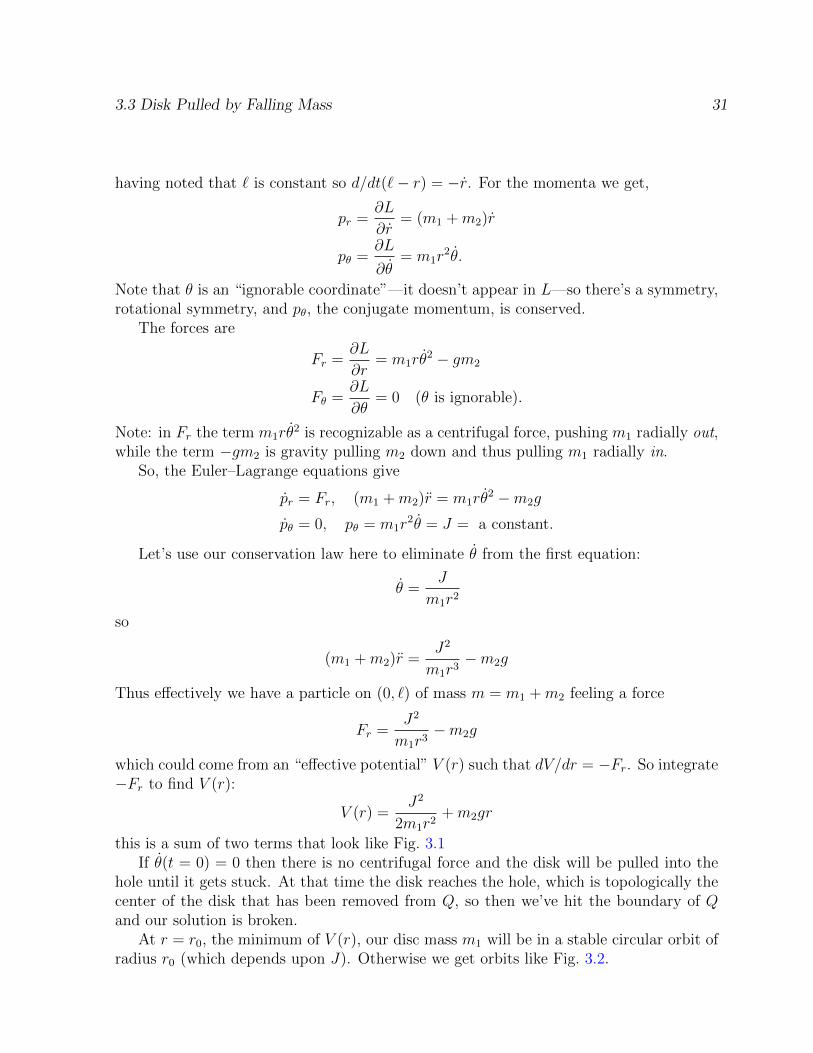
which could come from an “effective potential” V (r) such that dV/dr = −Fr. So integrate−Fr to find V (r):

V (r) =J2

2m1r2+m2gr

this is a sum of two terms that look like Fig. 3.1If θ(t = 0) = 0 then there is no centrifugal force and the disk will be pulled into the

hole until it gets stuck. At that time the disk reaches the hole, which is topologically thecenter of the disk that has been removed from Q, so then we’ve hit the boundary of Qand our solution is broken.

At r = r0, the minimum of V (r), our disc mass m1 will be in a stable circular orbit ofradius r0 (which depends upon J). Otherwise we get orbits like Fig. 3.2.

32 Examples

r0

V(r)

attractive grav. potnl

repulsive centrifugal

r

Figure 3.1: Potential function for disk pulled by gravitating mass.

Figure 3.2: Orbits for the disc and gravitating mass system.

3.4 Free Particle in Special Relativity

In relativistic dynamics the parameter coordinate that parametrizes the particle’s pathin Minkowski spacetime need not be the “time coordinate”, indeed in special relativitythere are many allowed time coordinates.

Minkowski spacetime is,Rn+1 3 (x0, x1, . . . , xn)

if space is n-dimensional. We normally take x0 as “time”, and (x1, . . . , xn) as “space”,but of course this is all relative to one’s reference frame. Someone else traveling at somehigh velocity relative to us will have to make a Lorentz transformation to translate fromour coordinates to theirs.

This has a Lorentzian metric

g(v, w) = v0w0 − v1w1 − . . .− vnwn

= ηµνvµwν

3.4 Free Particle in Special Relativity 33

where

ηµν =

1 0 0 . . . 00 −1 0 . . . 00 0 −1 0...

.... . .

...0 0 0 . . . −1

.

In special relativity we take spacetime to be the configuration space of a single pointparticle, so we let Q be Minkowski spacetime, i.e., Rn+1 3 (x0, . . . , xn) with the metricηµν defined above. Then the path of the particle is,

q : R(3 t) −→ Q

where t is a completely arbitrary parameter for the path, not necessarily x0, and notnecessarily proper time either. We want some Lagrangian L : TQ → R, i.e., L(qi, qi)such that the Euler–Lagrange equations will dictate how our free particle moves at aconstant velocity. Many Lagrangians do this, but the “best” one should give an actionthat is independent of the parameterization of the path—since the parameterization is“unphysical”: it can’t be measured. So the action

S(q) =

∫ t1

t0

L(qi(t), qi(t)

)dt

for q : [t0, t1]→ Q, should be independent of t. The obvious candidate for S is mass timesarclength,

S = m

∫ t1

t0

√ηij qi(t)qj(t) dt

or rather the Minkowski analogue of arclength, called proper time, at least when q isa timelike vector, i.e., ηij q

iqj > 0, which says q points into the future (or past) lightconeand makes S real, in fact it’s then the time ticked off by a clock moving along the path q :[t0, t1]→ Q. By “obvious candidate” we are appealing somewhat to physical intuition and

Lightlike

Timelike

Spacelike

generalization. In Euclidean space, free particles follow straight paths, so the arclengthor pathlength variation is an extremum, and we expect the same behavior in Minkowski

34 Examples

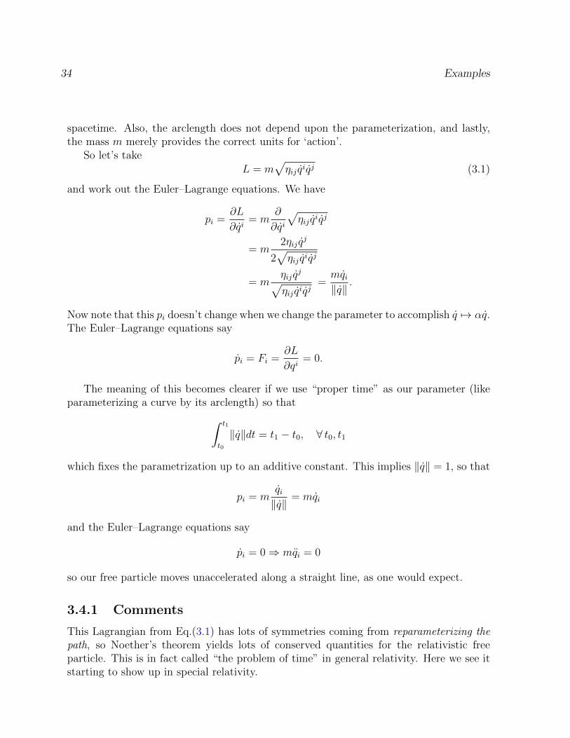
spacetime. Also, the arclength does not depend upon the parameterization, and lastly,the mass m merely provides the correct units for ‘action’.

So let’s takeL = m

√ηij qiqj (3.1)

and work out the Euler–Lagrange equations. We have

pi =∂L

∂qi= m

∂

∂qi

√ηij qiqj

= m2ηij q

j

2√ηij qiqj

= mηij q

j√ηij qiqj

=mqi‖q‖

.

Now note that this pi doesn’t change when we change the parameter to accomplish q 7→ αq.The Euler–Lagrange equations say

pi = Fi =∂L

∂qi= 0.

The meaning of this becomes clearer if we use “proper time” as our parameter (likeparameterizing a curve by its arclength) so that∫ t1

t0

‖q‖dt = t1 − t0, ∀ t0, t1

which fixes the parametrization up to an additive constant. This implies ‖q‖ = 1, so that

pi = mqi‖q‖

= mqi

and the Euler–Lagrange equations say

pi = 0⇒ mqi = 0

so our free particle moves unaccelerated along a straight line, as one would expect.

3.4.1 Comments

This Lagrangian from Eq.(3.1) has lots of symmetries coming from reparameterizing thepath, so Noether’s theorem yields lots of conserved quantities for the relativistic freeparticle. This is in fact called “the problem of time” in general relativity. Here we see itstarting to show up in special relativity.

3.4 Free Particle in Special Relativity 35

These reparameterization symmetries work as follows. Consider any (smooth) 1-parameter family of reparameterizations, i.e., diffeomorphisms

fs : R −→ R

with f0 = 1R. These act on the space of paths Γ = {q : R → Q} as follows: given anyq ∈ Γ we get

qs(t) = q(fs(t)

)where we should note that qs is physically indistinguishable from q. Let’s show that

δL = ˙, (when Euler–Lagrange eqns. hold)

so that Noether’s theorem gives a conserved quantity

piδqi − `

Here we go then:

δL =∂L

∂qiδqi +

∂L

∂qiδqi

= piδqi

=mqi‖q‖

d

dsqi(fs(t)

)∣∣∣∣s=0

=mqi‖q‖

d

dt

d

dsqi(fs(t)

)∣∣∣∣s=0

=mqi‖q‖

d

dtqi(fs(t)

)fs(t)ds

∣∣∣∣s=0

=mqi‖q‖

d

dt

(qiδfs

)=

d

dt

(piq

iδf)

where in the last step we used the Euler–Lagrange equations, i.e. ddtpi = 0, so δL = ˙ with

` = piqiδf .

So to recap a little: we saw the free relativistic particle has

L = m‖q‖ = m√ηij qiqj

and we’ve considered reparameterization symmetries

qs(t) = q(fs(t)

), fs : R→ R

36 Examples

we’ve used the fact that

δqi =d

dsqi(fs(t)

)∣∣∣∣s=0

= qiδf

so (repeating a bit of the above)

δL =∂L

∂qiδqi +

∂L

∂qiδqi

= piδqi, (since ∂L/∂qi = 0, and ∂L/∂qi = p)

= piδqi

= pid

dtδqi

= pid

dtqiδf

=d

dtpiq

iδf, and set piqiδf = `

so Noether’s theorem gives a conserved quantity

piδqi − ` = piq

iδf − piqiδf= 0

So these conserved quantities vanish! In short, we’re seeing an example of whatphysicists call gauge symmetries. This is a good topic for starting a new section.

3.5 Gauge Symmetries

What are gauge symmetries?

1. These are symmetries that permute different mathematical descriptions of the samephysical situation—in this case reparameterizations of a path.

2. These symmetries make it impossible to compute q(t) given q(0) and q(0): since ifq(t) is a solution so is q(f(t)) for any reparameterization f : R → R. We have ahigh degree of non-uniqueness of solutions to the Euler–Lagrange equations.

3. These symmetries give conserved quantities that work out to equal zero!

Note that (1) is a subjective criterion, (2) and (3) are objective, and (3) is easy totest, so we often use (3) to distinguish gauge symmetries from physical symmetries.

3.5 Gauge Symmetries 37

3.5.1 Relativistic Hamiltonian

What then is the Hamiltonian for special relativity theory? We’re continuing here withthe example problem of §3.4. Well, the Hamiltonian comes from Noether’s theorem fromtime translation symmetry,

qs(t) = q(t+ s)

and this is an example of a reparametrization (with δf = 1), so we see from the previousresults that the Hamiltonian is zero!

H = 0.

Explicitly, H = piδqi − ` where under q(t) → q(t + s) we have δqi = qiδf , and so

δL = d`/dt, which implies ` = piδqi. The result H = 0 follows.

Now you know why people talk about “the problem of time” in general relativitytheory, its glimmerings are seen in the flat Minkowski spacetime of special relativity. Youmay think it’s nice and simple to have H = 0, but in fact it means that there is notemporal evolution possible! So we can’t establish a dynamical theory on this footing!That’s bad news. (Because it means you might have to solve the static equations for the4D universe as a whole, and that’s impossible!)

But there is another conserved quantity deserving the title of “energy” which is notzero, and it comes from the symmetry,

qs(t) = q(t) + sw

where w ∈ Rn+1 and w points in some timelike direction.

qs

q

w

In fact any vector w gives a conserved quantity,

δL =∂L

∂qiδqi +

∂L

∂qiδqi

= piδqi, (since ∂L/∂qi = 0 and ∂L/∂qi = pi)

= pi0 = 0

38 Examples

since δqi = wi, δqi = wi = 0. This is our ˙ from Noether’s theorem with ` = 0, soNoether’s theorem says that we get a conserved quantity

piδqi − ` = piw

i

namely, the momentum in the w direction. We know p = 0 from the Euler–Lagrangeequations, for our free particle, but here we see it coming from spacetime translationsymmetry:

p =(p0, p1, . . . , pn)

p0 is energy, (p1, . . . , pn) is spatial momentum.

We’ve just about exhausted all the basic stuff that we can learn from the free particle.So next we’ll add some external force via an electromagnetic field.

3.6 Relativistic Particle in an Electromagnetic Field

The electromagnetic field is described by a 1-form A on spacetime, A is the vectorpotential, such that

dA = F (3.2)

is a 2-form containing the electric and magnetic fields,

Fij =∂Aj∂xi− ∂Ai∂xj

(3.3)

We can write (for Q having local charts to Rn+1),

A = A0dx0 + A1dx

1 + . . . Andxn

and then because d2 = 0

dA = dA0dx0 + dA1dx

1 + . . . dAndxn

and since the Aj are just functions,

dAj = ∂iAjdxi

using the summation convention and ∂i := ∂/∂xi. The reader can easily check that thecomponents for F = F01dx

0 ∧ dx1 +F02dx0 ∧ dx2 + . . ., agrees with the matrix expression

below (at least in 4 dimensions).So, for example, in 4-dimensional spacetime

F =

0 E1 E2 E3

−E1 0 B3 −B2

−E2 −B3 0 B1

−E3 B2 −B1 0

3.6 Relativistic Particle in an Electromagnetic Field 39

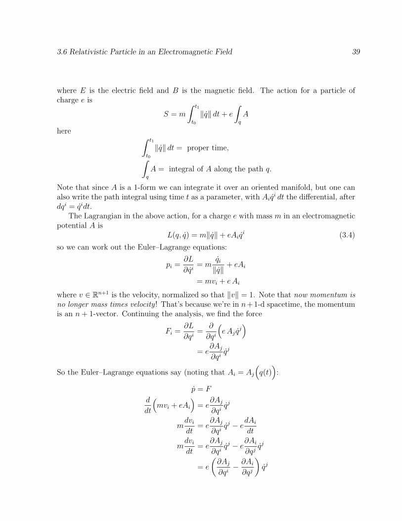
where E is the electric field and B is the magnetic field. The action for a particle ofcharge e is

S = m

∫ t1

t0

‖q‖ dt+ e

∫q

A

here ∫ t1

t0

‖q‖ dt = proper time,∫q

A = integral of A along the path q.

Note that since A is a 1-form we can integrate it over an oriented manifold, but one canalso write the path integral using time t as a parameter, with Aiq

i dt the differential, afterdqi = qidt.

The Lagrangian in the above action, for a charge e with mass m in an electromagneticpotential A is

L(q, q) = m‖q‖+ eAiqi (3.4)

so we can work out the Euler–Lagrange equations:

pi =∂L

∂qi= m

qi‖q‖

+ eAi

= mvi + eAi

where v ∈ Rn+1 is the velocity, normalized so that ‖v‖ = 1. Note that now momentum isno longer mass times velocity ! That’s because we’re in n+ 1-d spacetime, the momentumis an n+ 1-vector. Continuing the analysis, we find the force

Fi =∂L

∂qi=

∂

∂qi

(eAj q

j)

= e∂Aj∂qi

qj

So the Euler–Lagrange equations say (noting that Ai = Aj

(q(t)

):

p = F

d

dt

(mvi + eAi

)= e

∂Aj∂qi

qj

mdvidt

= e∂Aj∂qi

qj − edAidt

mdvidt

= e∂Aj∂qi

qj − e∂Ai∂qj

qj

= e

(∂Aj∂qi− ∂Ai∂qj

)qj

40 Examples

the term in parentheses is F ij = the electromagnetic field, F = dA. So we get the followingequations of motion

mdvidt

= eF ij qj, (Lorentz force law) (3.5)

(Usually called the “Lorenz” force law.)

3.7 Lagrangian for a String

So we’ve looked at a point particle and tried

S = m · (arclength) +

∫A

or with ‘proper time’ instead of ‘arclength’, where the 1-from A can be integrated overa 1-dimensional path. A generalization (or specialization, depending on how you look atit) would be to consider a Lagrangian for an extended object.

In string theory we boost the dimension by +1 and consider a string tracing out a 2Dsurface as time passes (Fig. 3.3).

becomes

Figure 3.3: Worldtube of a closed string.

Can you infer an appropriate action for this system? Remember, the physical orphysico-philosophical principle we’ve been using is that the path followed by physicalobjects minimizes the “activity” or “aliveness” of the system. Given that we presumablycannot tamper with the length of the closed string, then the worldtube quantity analogousto arclength or proper time would be the area of the worldtube (or worldsheet for an openstring). If the string is also assumed to be a source of electromagnetic field then we needa 2-form to integrate over the 2D worldtube analogous to the 1-form integrated over thepathline of the point particle. In string theory this is usually the “Kalb-Ramond field”,

3.8 Another Lagrangian for Relativistic Electrodynamics 41

call it B. To recover electrodynamic interactions it should be antisymmetric like A, butits tensor components will have two indices since it’s a 2-form. The string action can thenbe written

S = α · (area) + e

∫B (3.6)

We’ve also replaced the point particle mass by the string tension α [mass·length−1] toobtain the correct units for the action (since replacing arclength by area meant we had tocompensate for the extra length dimension in the first term of the above string action).

This may still seem like we’ve pulled a rabbit out of a hat. But we haven’t checked thatthis action yields sensible dynamics yet! But supposing it does, then would it justify ourguesswork and intuition in arriving at Eq.(3.6)? Well by now you’ve probably realizedthat one can have more than one form of action or Lagrangian that yields the samedynamics. So provided we supply reasonabe physically realistic heuristics then whateverLagrangian or action that we come up with will stand a good chance of describing somesystem with a healthy measure of physical verisimilitude.

That’s enough about string for now. The point was to illustrate the type of reasoningthat one can use in conjuring up a Lagrangian. It’s particularly useful when Newtoniantheory cannot give us a head start, i.e., in relativistic dynamics and in the physics ofextended particles.

3.8 Another Lagrangian for Relativistic Electrody-

namics

In § 3.6, Eq.(3.4) we saw an example of a Lagrangian for relativistic electrodynamicsthat had awkward reparametrization symmetries, meaning that H = 0 and there werenon-unique solutions to the Euler–Lagrange equations arising from applying gauge trans-formations. This freedom to change the gauge can be avoided.

Recall Eq.(3.4), which was a Lagrangian for a charged particle with reparametrizationsymmetry

L = m‖q‖+ eAiqi

just as for an uncharged relativistic particle. But there’s another Lagrangian we can usethat doesn’t have this gauge symmetry:

L =1

2mq · q + eAiq

i (3.7)

This one even has some nice features.

• It looks formally like “12mv2”, familiar from nonrelativistic mechanics.

• There’s no ugly square root, so it’s everywhere differentiable, and there’s no troublewith paths being timelike or spacelike in direction, they are handled the same.

42 Examples

What Euler–Lagrange equations does this Lagrangian yield?

pi =∂L

∂qi= mqi + eAi

Fi =∂L

∂qi= e

∂Aj∂qi

qj

Very similar to before! The Euler–Lagrange equations then say

d

dt

(mqi + eAi

)= e

∂Aj∂qi

qj

mqi = eF ij qj

almost as before. (I’ve taken to using F here for the electromagnetic field tensor to avoidclashing with F for the generalized force.) The only difference is that we have mqi insteadof mvi where vi = qi/‖q‖. So the old Euler–Lagrange equations of motion reduce to thenew ones if we pick a parametrization with ‖q‖ = 1, which would be a parametrizationby proper time for example.

Let’s work out the Hamiltonian for this

L =1

2mq · q + eAiq

i

for the relativistic charged particle in an electromagnetic field. Recall that for ourreparametrization-invariant Lagrangian

L = m√qiqi + eAiq

i

we got H = 0, time translation was a gauge symmetry. With the new Lagrangian it’snot! Indeed

H = piqi − L

and now

pi =∂L

∂qi= mqi + eAi

so

H = (mqi + eAi)qi − (1

2mqiq

i + eAiqi)

= 12mqiq

i

3.8 Another Lagrangian for Relativistic Electrodynamics 43

Comments. This is vaguely like how a nonrelativistic particle in a potential V has

H = piqi − L = 2K − (K − V ) = K + V,

but now the “potential’ V = eAiqi is linear in velocity, so now

H = piqi − L = (2K − V )− (K − V ) = K.

As claimed H is not zero, and the fact that it’s conserved says ‖q(t)‖ is constant asa function of t, so the particle’s path is parameterized by proper time up to rescalingof t. That is, we’re getting “conservation of speed” rather than some more familiar“conservation of energy”. The reason is that this Hamiltonian comes from the symmetry

qs(t) = q(t+ s)

instead of spacetime translation symmetry

qs(t) = q(t) + sw, w ∈ Rn+1

the difference is illustrated schematically in Fig. 3.4.

w

qs=q(t+s) qs=q+sw

0

12

3

4

12

3

4

5

Figure 3.4: Proper time rescaling vs spacetime translation.

Our LagrangianL(q, q) = 1

2m‖q‖2 + Ai(q)q

i

has time translation symmetry iff A is translation invariant (but it’s highly unlikely agiven system of interest will have A(q) = A(q+sw)). In general then there’s no conserved“energy” for our particle corresponding to translations in time.

44 Examples

3.9 The Free Particle in General Relativity

In general relativity, spacetime is an (n + 1)-dimensional Lorentzian manifold, namely asmooth (n+ 1)-dimensional manifold Q with a Lorentzian metric g. We define the metricas follows.

1. For each x ∈ Q, we have a bilinear map

g(x) : TxQ× TxQ −→ R(v, w) 7−→ g(x)(v, w)

or we could write g(v, w) for short.

2. With respect to some basis of TxQ we have

g(v, w) = gijviwj

gij =

1 0 . . . 00 −1 0...

. . ....

0 0 . . . −1

Of course we can write g(v, w) = gijv

iwj in any basis, but for different bases gij willhave a different form.

3. g(x) varies smoothly with x.

The Lagrangian for a free point particle in the spacetime Q is

L(q, q) = m√g(q)(q, q)

= m√gij qiqj

just like in special relativity but with ηij replaced by gij. Alternatively we could just aswell use

L(q, q) = 12mg(q)(q, q)

= 12mgij q

iqj

The big difference between these two Lagrangians is that now spacetime translationsymmetry (and rotation, and boost symmetry) is gone! So there is no conserved energy-momentum (nor angular momentum, nor velocity of center of energy) anymore!

Let’s find the equations of motion. Suppose then Q is a Lorentzian manifold withmetric g and L : TQ→ R is the Lagrangian of a free particle,

L(q, q) = 12mgij q

iqj

3.9 The Free Particle in General Relativity 45

We find equations of motion from the Euler–Lagrange equations, which in this case startfrom

pi =∂L

∂qi= mgij q

j

The velocity q here is a tangent vector, the momentum p is a cotangent vector, and weneed the metric to relate them, via

g : TqM× TqM−→ R(v, w) 7−→ g(v, w)

which gives

TqM−→ T ∗qMv 7−→ g(v,−).

In coordinates this would say that the tangent vector vi gets mapped to the cotangentvector gijv

j. This is lurking behind the passage from qi to the momentum mgijvj.

Getting back to the Euler–Lagrange equations,

pi =∂L

∂qi= mgij q

j

Fi =∂L

∂qi=

∂

∂qi

(12mgjk(q)q

j qk)

= 12m∂igjkq

j qk, (where ∂i =∂

∂qi).

So the Euler–Lagrange equations say

d

dtmgij q

j = 12m∂igjkq

j qk.

The mass factors away, so the motion is independent of the mass! Essentially we have ageodesic equation.

We can rewrite this geodesic equation as follows

d

dtgij q

j = 12∂igjkq

j qk

∴ ∂kgij qkqj + gij q

j = 12∂igjkq

j qk

∴ gij qj =

(12∂igjk − ∂kgij

)qj qk

= 12

(∂igjk − ∂kgij − ∂jgki

)qj qk

where the last line follows by symmetry of the metric, gik = gki. Now let,

Γijk = −(∂igjk − ∂kgij − ∂jgki

)

46 Examples

the minus sign being just a convention (so that we agree with everyone else). This defineswhat we call the Christoffel symbols Γijk. Then

qi = gij qj = −Γijkq

j qk

∴ qi = −Γijkqj qk.

So we see that q can be computed in terms of q and the Christoffel symbols Γijk, which isreally a particular type of connection that a Lorentzian manifold has (the Levi-Civita con-nection), a “connection” is just the rule for parallel transporting tangent vectors aroundthe manifold.

Parallel transport is just the simplest way to compare vectors at different points inthe manifold. This allows us to define, among other things, a “covariant derivative”.

3.10 A Charged Particle on a Curved Spacetime

We can now apply what we’ve learned in consideration of a charged particle, of charge e,in an electromagnetic field with potential A, in our Lorentzian manifold. The Lagrangianwould be

L = 12mgjkq

j qk + eAiqi

which again was conjured up be replacing the flat space metric ηij by the metric for GRgij. Not surprisingly, the Euler–Lagrange equations then yield the following equations ofmotion,

mqi = −mΓijkqj qk + eF ij q

j.

If you want to know more about Lagrangians for general relativity we recommend thepaper by Peldan [Pel94], and also the “black book” of Misner, Thorne & Wheeler [WTM71].

3.11 The Principle of Least Action and Geodesics

3.11.1 Jacobi and Least Time vs Least Action

We’ve mentioned that Fermat’s principle of least time in optics is analogous to the prin-ciple of least action in particle mechanics. This analogy is strange, since in the principleof least action we fix the time interval q : [0, 1] → Q. Also, if one imagines a force on aparticle resulting from a potential gradient at an interface as analogous to light refractionthen you also get a screw-up in the analogy (Fig. 3.5).

Nevertheless, Jacobi was able to reinterpret the mechanics of a particle as an opticsproblem and hence “unify” the two minimization principles. First, let’s consider light ina medium with a varying index of refraction n (recall 1/n ∝ speed of light). Suppose

3.11 The Principle of Least Action and Geodesics 47

light

light

faster

slower

particle

particle

slower

faster

n high

n low

V high

V low

Figure 3.5: Least time versus least action.

it’s in Rn with its usual Euclidean metric. If the light is trying to minimize the time, itstrying to minimize the arclength of its path in the metric

gij = n2δij

that is, the index of refraction n : Rn → (0,∞), times the usual Euclidean metric

δij =

1 0

. . .

0 1

This is just like the free particle in general relativity (minimizing its proper time)

except that now gij is a Riemannian metric

g(v, w) = gijviwj

where g(v, v) ≥ 0

So we’ll use the same Lagrangian:

L(q, q) =√gij(q)qiqj

and get the same Euler–Lagrange equations:

d2qi

dt2+ Γijkq

j qk = 0 (3.8)

if q is parameterized by arclength or more generally

‖q‖ =√gij(q)qiqj = constant.

48 Examples

As before the Christoffel symbols Γ are built from the derivatives of the metric g.Now, what Jacobi did is show how the motion of a particle in a potential could be

viewed as a special case of this. Consider a particle of mass m in Euclidean Rn withpotential V : Rn → R. It satisfies F = ma, i.e.,

md2qi

dt2= −∂iV (3.9)

How did Jacobi see (3.9) as a special case of (3.8)? He considered a particle of energy Eand he chose the index of refraction to be

n(q) =

√2

m

(E − V (q)

)which is just the speed of a particle of energy E when the potential energy is V (q), since√

2

m(E − V ) =

√2

m

1

2m‖q‖2 = ‖q‖.

Note: this is precisely backwards compared to optics, where n(q) is proportional to thereciprocal of the speed of light!! But let’s see that it works.

L =√gij(q)qiqj

=√n2(q)qiqj

=√

2/m(E − V (q))q2

where q2 = q · q is just the usual Euclidean dot product, v · w = δijviwj. We get the

Euler–Lagrange equations,

pi =∂L

∂qi=

√2

m(E − V ) · q

‖q‖

Fi =∂L

∂qi= ∂i

√2

m(E − V (q)) · ‖q‖

=1

2

−2/m∂iV√2/m(E − V q)

· ‖q‖

Then p = F says,

d

dt

√2/m(E − V (q)) · qi

‖q‖= − 1

m∂iV

‖q‖√2/m(E − V )

Jacobi noticed that this is just F = ma, or mqi = −∂iV , that is, provided we reparame-terize q so that,

‖q‖ =√

2/m(E − V (q)).

Recall that our Lagrangian gives reparameterization invariant Euler–Lagrange equations!This is the unification between least time (from optics) and least action (from mechanics)that we sought.


3.11.2 The Ubiquity of Geodesic Motion

We’ve seen that many classical systems trace out paths that are geodesics, i.e., pathsq : [t0, t1]→ Q that are critical points of

S(q) =

∫ t1

t0

√gij qiqj dt

which is proper time when (Q, g) is a Lorentzian manifold, or arclength when (Q, g) is aRiemannian manifold. We have

1. The metric at q ∈ Q is,

g(q) : TqQ× TqQ→ R(v, w) 7→ g(v, w)

and it is bilinear.

2. w.r.t a basis of TqQg(v, w) = δijv

iwj

3. g(q) varies smoothly with q ∈ Q.

An important distinction to keep in mind is that Lorentzian manifolds represent space-times, whereas Riemannian manifolds represent that we’d normally consider as just space.

We’ve seen at least three important things.

(1) In the geometric optics approximation, light in Q = Rn acts like particles tracingout geodesics in the metric

gij = n(q)2δij

where n : Q→ (0,∞) is the index of refraction function.

(2) Jacobi saw that a particle in Q = Rn in some potential V : Q → R traces outgeodesics in the metric

gij =2

m(E − V )δij

if the particle has energy E (where1 V < E).

(3) A free particle in general relativity traces out a geodesic on a Lorentzian manifold(Q, q).

In fact all three of these results can be generalized to cover every problem that we’vediscussed!

1The case V > E, if they exist, would be classically forbidden regions.

50 Examples

(1′) Light on any Riemannian manifold (Q, q) with index of refraction n : Q → (0,∞)traces out geodesics in the metric h = n2g.

(2′) A particle on a Riemannian manifold (Q, q) with potential V : Q → R traces outgeodesics w.r.t the metric

h =2

m(E − V )g

if it has energy E. Lots of physical systems can be described this way, e.g., theAtwood machine, a rigid rotating body (Q = SO(3)), spinning tops, and others.All of these systems have a Lagrangian which is a quadratic function of position, sothey all fit into this framework.

(3′) Kaluza-Klein Theory. A particle with charge e on a Lorentzian manifold (Q, q)in an electromagnetic vector potential follows a path with

qi = −Γijkqj qk +

e

mF ij q

j

whereF ij = ∂iAj − ∂jAi

but this is actually geodesic motion on the manifold Q× U(1) where U(1) = {eiθ :θ ∈ R} is a circle.

Let’s examine this last result a bit further. To get the desired equations for motion onQ×U(1) we need to given Q×U(1) a cleverly designed metric built from g and A wherethe amount of “spiralling”—the velocity in the U(1) direction is e/m. The metric h on

QxU(1)

a geodesic

Q

the apparent

Q×U(1) is built from g and A in a very simple way. Let’s pick coordinates xi on Q wherei ∈ {0, . . . , n} since we’re in n + 1-dimensional spacetime, and θ is our local coordinateon S1. The components of h are

hij = gij + AiAj

hθi = hθi = −Aihθθ = 1


Working out the equations for a geodesic in this metric we get

qi = −Γijkqj qk +

e

mF ij q

j

qθ = 0,

if qθ = e/m. Since F ij is part of the Christoffel symbols for h.To summarize this section on least time versus least action we can say that every

problem that we’ve discussed in classical mechanics can be regarded as geodesic motion!

52 Examples

Chapter 4

From Lagrangians to Hamiltonians

In the Lagrangian approach we focus on the position and velocity of a particle, andcompute what the particle does starting from the Lagrangian L(q, q), which is a function

L : TQ −→ R

where the tangent bundle is the space of position-velocity pairs. But we’re led toconsider momentum

pi =∂L

∂qi

since the equations of motion tell us how it changes:

dpidt

=∂L

∂qi.

4.1 The Hamiltonian Approach

In the Hamiltonian approach we focus on position and momentum, and compute whatthe particle does starting from the energy

H = piqi − L(q, q)

reinterpreted as a function of position and momentum We call this the Hamiltonian

H : T ∗Q −→ R

where the cotangent bundle is the space of position-momentum pairs. In this approach,position and momentum will satisfy Hamilton’s equations:

dqi

dt=∂H

∂pi,

dpi

dt= −∂H

∂qi

53

54 From Lagrangians to Hamiltonians

where the latter is the Euler–Lagrange equation

dpi

dt=∂L

∂qi

in disguise (it has a minus sign since H = pq − L).To obtain this Hamiltonian description of mechanics rigorously we need to study this

map

λ : TQ −→ T ∗Q

(q, q) 7−→ (q, p)

where q ∈ Q, and q is any tangent vector in TqQ (not the time derivative of something),and p is a cotangent vector in T ∗qQ := (TqQ)∗, given by

qλ−→ pi =

∂L

∂qi.

So λ is defined using L : TQ→ R. Despite appearances, λ can be defined in a coordinate-free way, as follows (referring to Fig. ??). To understand “ ∂L

∂qi” in a coordinate-free way,

TqQ

TQ

T(q,qdot)TqQ

QTqQ

q

Figure 4.1:

we treat it as the “differential of L in the vertical direction”—i.e., the qi directions. Todo this, note that the differential of

π : TQ −→ Q(q, q) 7−→ q

is a mapdπ : TTQ −→ TQ.

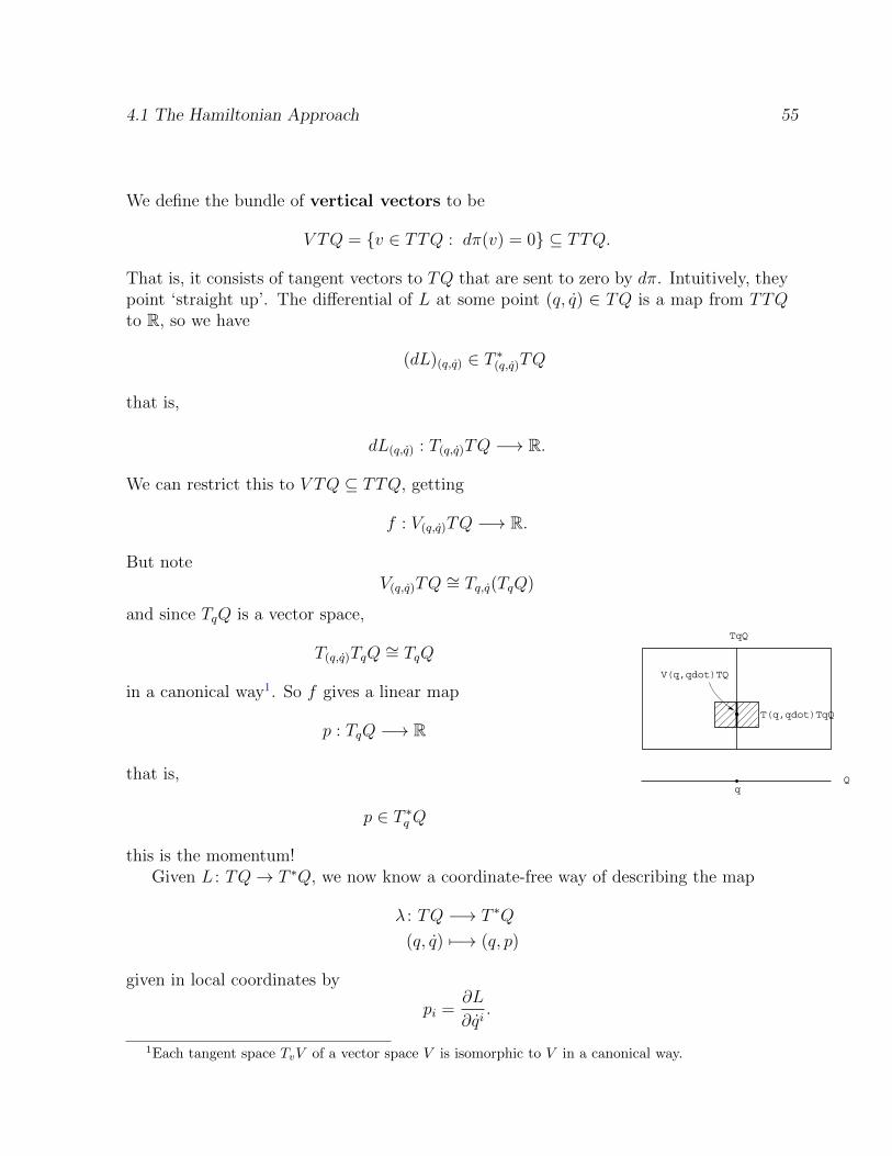
4.1 The Hamiltonian Approach 55

We define the bundle of vertical vectors to be

V TQ = {v ∈ TTQ : dπ(v) = 0} ⊆ TTQ.

That is, it consists of tangent vectors to TQ that are sent to zero by dπ. Intuitively, theypoint ‘straight up’. The differential of L at some point (q, q) ∈ TQ is a map from TTQto R, so we have

(dL)(q,q) ∈ T ∗(q,q)TQ

that is,

dL(q,q) : T(q,q)TQ −→ R.

We can restrict this to V TQ ⊆ TTQ, getting

f : V(q,q)TQ −→ R.

But noteV(q,q)TQ ∼= Tq,q(TqQ)

TqQ

T(q,qdot)TqQ

Qq

V(q,qdot)TQ

and since TqQ is a vector space,

T(q,q)TqQ ∼= TqQ

in a canonical way1. So f gives a linear map

p : TqQ −→ R

that is,

p ∈ T ∗qQ

this is the momentum!Given L : TQ→ T ∗Q, we now know a coordinate-free way of describing the map

λ : TQ −→ T ∗Q

(q, q) 7−→ (q, p)

given in local coordinates by

pi =∂L

∂qi.

1Each tangent space TvV of a vector space V is isomorphic to V in a canonical way.


We say L is regular if λ is a diffeomorphism from TQ to some open subset X ⊆ T ∗Q.In this case we can describe what our system is doing equally well by specifying positionand velocity,

(q, q) ∈ TQ

or position and momentum(q, p) = λ(q, q) ∈ X.

We call X the phase space of the system. In practice often X = T ∗Q, then L is said tobe strongly regular.

4.2 Regular and Strongly Regular Lagrangians

This section discusses some examples of the above theory.

4.2.1 Example: A Particle in a Riemannian Manifold with Po-tential V (q)

For a particle in a Riemannian manifold (Q, q) in a potential V : Q→ R has Lagrangian

L(q, q) =1

2mgij q

iqj − V (q)

Here

pi =∂L

∂qi= mgij q

j

soλ(q, q) =

(q,mg(q,−)

)L is strongly regular in this case because

TqQ −→ T ∗qQ

v −→ g(v,−)

is 1-1 and onto, i.e., the metric is nondegenerate. Thus λ is a diffeomorphism, which inthis case extends to all of T ∗Q.

4.2.2 Example: General Relativistic Particle in an E-M Poten-tial

For a general relativistic particle with charge e in an electromagnetic vector potential Athe Lagrangian is

L(q, q) =1

2mgij q

iqj − eAiqi

4.2 Regular and Strongly Regular Lagrangians 57

and thus

pi =∂L

∂qi= mgij q

iqj + eAi.

This L is still strongly regular, but now each map

λ |TqQ : TqQ −→ T ∗qQ

q 7−→ mg(q,−) + eA(q)

is affine rather than linear2.

4.2.3 Example: Free General Relativistic Particle with Repa-rameterization Invariance

The free general relativistic particle with reparameterization invariant Lagrangian has

L(q, q) = m√gij qiqj.

This is terrible from the perspective of regularity—it’s not differentiable when gij qiqj

vanishes, and undefined when the same is negative. Where it is defined

pi =∂L

∂qi=mgij q

j

‖q‖

(where q is timelike), we can ask about regularity. Alas, the map λ is not 1-1 where definedsince multiplying q by some number has no effect on p! (This is related to the reparameter-ization invariance—this always happens with reparameterization-invariant Lagrangians.)

4.2.4 Example: A Regular but not Strongly Regular Lagrangian

Here’s a Lagrangian that’s regular but not strongly regular. Let Q = R and

L(q, q) = f(q)

so that

p =∂L

∂q= f ′(q)

This will be regular but not strongly so if f ′ : R→ R is a diffeomorphism from R to someproper subset U ⊂ R. For example, take f(q) = eq so f ′ : R ∼→ (0,∞) ⊂ R. So

L(q, q) = eq //

positive slope

2All linear transforms are affine, but affine transformations include translations, which are nonlinear.In affine geometry there is no defined origin. For the example the translation is the “+eA(q)” part.


or

L(q, q) =√

1 + q2 //

slope between−1 and 1

and so forth.

4.3 Hamilton’s Equations

Now let’s assume L is regular, so

λ : TQ −→ X ⊆ T ∗Q

(q, q) 7−→ (q, p)

is a diffeomorphism. This lets us have the best of both worlds: we can identify TQ withX using λ. This lets us treat qi, pi, L, H, etc., all as functions on X (or TQ), thus writing

qi (function on TQ)

for the function

qi ◦ λ−1 (function on X)

In particular

pi :=∂L

∂qi(Euler–Lagrange equation)

which is really a function on TQ, will be treated as a function on X. Now let’s calculate:

dL =∂L

∂qidqi +

∂L

∂qidqi

= pidqi + pidq

i

while

dH = d(piqi − L)

= qidpi + pidqi − dL

= qidpi + pidqi − (pidq

i + pidqi)

= qidpi − pidqi

sodH = qidpi − pidqi.

4.3 Hamilton’s Equations 59

Assume the Lagrangian L : TQ→ R is regular, so

λ : TQ∼−→ X ⊆ T ∗Q

(q, q) 7−→ (q, p)

is a diffeomorphism. This lets us regard both L and the Hamiltonian H = piqi − L as

functions on the phase space X, and use (qi, qi) as local coordinates on X. As we’ve seen,this gives us

dL = pidqi + pidq

i

dH = qidpi − pidqi.

But we can also work out dH directly, this time using local coordinates (qi, pi), to get

dH =∂H

∂pidpi +

∂H

∂qidqi.

Since dpi, dqi form a basis of 1-forms, we conclude:

qi =∂H

∂pi, pi = −∂H

∂qi

These are Hamilton’s Equations.

4.3.1 Hamilton and Euler–Lagrange

Though qi and pi are just functions of X, when the Euler–Lagrange equations hold forsome path q : [t0, t1] → Q, they will be the time derivatives of qi and pi. So whenthe Euler–Lagrange equations hold, Hamilton’s equations describe the motion of a pointx(t) =

(q(t), p(t)

)∈ X. In fact, in this context, Hamilton’s equations are just the Euler–

Lagrange equations in disguise. The equation

qi =∂H

∂pi

really just lets us recover the velocity q as a function of q and p, inverting the formula

pi =∂L

∂qi

which gave p as a function of q and q. So we get a formula for the map

λ−1 : X −→ TQ

(q, p) 7−→ (q, q).


Given this, the other Hamilton equation

pi = −∂H∂qi

is secretly the Euler–Lagrange equation

d

dt

∂L

∂qi=∂L

∂qi,

or pi = ∂L∂qi

for short. These are the same because

∂H

∂qi=

∂

∂qi(piq

i − L)

= −∂L∂qi

.

Example: Particle in a Potential V (q)

For a particle in Q = Rn in a potential V : Rn → R the system has Lagrangian

L(q, q) =m

2‖q‖2 − V (q)

which gives

p = mq

q =p

m, (though really that’s q =

gijpjm

)

and Hamiltonian

H(q, p) = piqi − L =

1

m‖p‖2 −

(‖p‖2

2m− V

)=

1

2m‖p‖2 + V (q).

So Hamilton’s equations say

qi =∂H

∂pi⇒ q =

p

m

pi = −∂H∂qi

⇒ p = −∇V

The first just recovers q as a function of p; the second is F = ma.

4.3 Hamilton’s Equations 61

Note on Symplectic Structure

Hamilton’s equations push us toward the viewpoint where p and q have equal status ascoordinates on the phase space X. Soon, we’ll drop the requirement that X ⊆ T ∗Q whereQ is a configuration space. X will just be a manifold equipped with enough structure towrite down Hamilton’s equations starting from any H : X → R.

The coordinate-free description of this structure is the major 20th century contributionto mechanics: a symplectic structure.

This is important. You might have some particles moving on a manifold like S3,which is not symplectic. So the Hamiltonian mechanics point of view says that theabstract manifold that you are really interested in is something different: it must be asymplectic manifold. That’s the phase space X. We’ll introduce symplectic geometrymore completely in later chapters.

4.3.2 Hamilton’s Equations from the Principle of Least Action

Before, we obtained the Euler–Lagrange equations by associating an “action” S withany q : [t0, t1] → Q and setting δS = 0. Now let’s get Hamilton’s equations directly byassigning an action S to any path x : [t0, t1] → X and setting δS = 0. Note: we don’timpose any relation between p and q, q! The relation will follow from δS = 0.

Let P be the space of paths in the phase space X and define the action

S : P −→ R

by

S(x) =

∫ t1

t0

(piqi −H)dt

since piqi −H is another way of writing the Lagrangian. More precisely, write our path

x as x(t) =(q(t), p(t)

)and let

S(x) =

∫ t1

t0

[pi(t)

d

dtqi(t)−H

(q(t), p(t)

)]dt

we write ddtqi instead of qi to emphasize that we mean the time derivative rather than a

coordinate in phase space.Let’s show δS = 0⇔Hamilton’s equations.

δS = δ

∫(piq

i −H)dt

=

∫ (δpiq

i + piδqi − δH

)dt


then integrating by parts,

=

∫ (δpiq

i − piδqi − δH)dt

=

∫ (δpiq

i − piδqi −∂H

∂qiδqi − ∂H

∂piδpi

)dt

=

∫ (δpi

(qi − ∂H

∂pi

)+ δqi

(−pi −

∂H

∂qi

))dt

This vanishes ∀δx = (δq, δp) if and only if Hamilton’s equations

qi =∂H

∂pi, pi = −∂H

∂qi

hold, just as we hoped.We’ve seen two principles of “least action”:

1. For paths in configuration space Q, δS = 0⇔Euler–Lagrange equations.

2. For paths in phase space X, δS = 0⇔Hamilton’s equations.

Additionally, since X ⊆ T ∗Q, we might consider a third version based on paths inposition-velocity space TQ. But when our Lagrangian is regular we have a diffeomor-phism λ : TQ

∼→ X, so this third principle of least action is just a reformulation ofprinciple 2. However, the really interesting principle of least action involves paths in theextended phase space where we have an additional coordinate for time: X × R.

Recall the action

S(x) =

∫(piq

i −H) dt

=

∫pidqi

dtdt−H dt

=

∫pidq

i −H dt

We can interpet the integrand as a 1-form

β = pidqi −H dt

on X × R, which has coordinates {pi, qi, t}. So any path

x : [t0, t1] −→ X

gives a path

σ : [t0, t1] −→ X × Rt 7−→ (x(t), t)

4.4 Waves versus Particles—The Hamilton-Jacobi Equations 63

and the action becomes the integral of a 1-form over a curve:

S(x) =

∫pi dq

i −H dt =

∫σ

β

4.4 Waves versus Particles—The Hamilton-Jacobi Equa-

tions

In quantum mechanics we discover that every particle—electrons, photons, neutrinos,etc.—is a wave, and vice versa. Interestingly Newton already had a particle theory oflight (his “corpuscules”) and various physicists argued against it by pointing out thatdiffraction is best explained by a wave theory. We’ve talked about geometrized optics, anapproximation in which light consists of particles moving along geodesics. Here we startwith a Riemannian manifold (Q, g) as space, but we use the new metric

hij = n2gij

where n : Q → (0,∞) is the index of refraction throughout space (generally not a con-stant).

4.4.1 Wave Equations

Huygens considered this same setup (in simpler language) and considered the motion ofa wavefront:

//


and saw that the wavefront is the envelope of a bunch of little wavelets centered at pointsalong the big wavefront:

balls of radius εcentered at points

of the old wavefront��

In short, the wavefront moves at unit speed in the normal direction with respect to the“optical metric” h. We can think about the distance function

d : Q×Q −→ [0,∞)

on the Riemannian manifold (Q, h), where

d(q0, q1) = infΥ

(arclength)

where Υ = {paths from q0 to q1}. (Secretly this d(q0, q1) is the least action—the infimumof action over all paths from q0 to q1.) Using this we get the wavefronts centered at q0 ∈ Qas the level sets

{q : d(q0, q) = c}

or at least for small c > 0, as depicted in Fig. 4.2. For larger c the level sets can ceaseto be smooth—we say a catastrophe occurs—and then the wavefronts are no longer thelevel sets. This sort of situation can happen for topological reasons (as when the wavessmash into each other in the back of Fig. 4.2) and it can also happen for geometricalreasons (Fig. 4.3). Assuming no such catastrophes occur, we can approximate the wavesof light by a wavefunction:

ψ(q) = A(q)eik d(q,q0)

where k is the wavenumber of the light (i.e., its color) and A : Q→ R describes the ampli-tude of the wave, which drops off far from q0. This becomes the eikonal approximationin optics3 once we figure out what A should be.

3Eikonal comes form the Greek word for ‘image’ or ‘likeness’, in optics the eikonal approximation isthe basis for ray tracing methods.


q0

Page 1 of 1

9/7/2019file:///D:/My%20Website/classical/texfiles/2005/book/images/wave-levelsets.svg

Figure 4.2:

Figure 4.3:

Hamilton and Jacobi focused on distance d : Q × Q → [0,∞) as a function of twovariables. This is now called Hamilton’s principal function, and we will denote it as W .They noticed that

∂

∂qi1W (q0, q1) = (p1)i

q0•

p1• //

q1

where p1 is a cotangent vector pointing normal to the wavefronts.


4.4.2 The Hamilton-Jacobi Equations

We’ve seen that in optics, particles of light move along geodesics, but wavefronts are levelsets of the distance functions:

88

at least while the level sets remain smooth. In the eikonal approximation, light is describedby waves

ψ : Q −→ Cψ(q1) = A(q1)eikW (q0,q1)

where (Q, h) is a Riemannian manifold, h is the optical metric, q0 ∈ Q is the light source,k is the frequency and

W : Q×Q −→ [0,∞)

is the distance function on Q, or Hamilton’s principal function:

W (q0, q1) = infq∈Υ

S(q)

where Υ is the space of paths from q0 to q and S(q) is the action of the path q, i.e., itsarclength. This is begging to be generalized to other Lagrangian systems! (At least it isretrospectively, with the advantage of our historical perspective.) We also saw that

∂

∂qi1W (q0, q1) = (p1)i,

q0•

p1• //

q1

“points normal to the wavefront”—really the tangent vector

pi1 = hij(p1)j

points in this direction. In fact kp1i is the momentum of the light passing through q1.This foreshadows quantum mechanics! After all, in quantum mechanics, the momentumis an operator that acts to differentiating the wavefunction.


Jacobi generalized this to the motion of point particles in a potential V : Q→ R, usingthe fact that a particle of energy E traces out geodesics in the metric

hij =2(E − V )

mgij.

We’ve seen this reduces point particle mechanics to optics—but only for particles of fixedenergy E. Hamilton went further, and we now can go further still.

Suppose Q is any manifold and L : TQ → R is any function (Lagrangian). DefineHamilton’s principal function

W : Q× R×Q× R −→ R

byW (q0, t0; q1, t1) = inf

q∈ΥS(q)

whereΥ =

{q : [t0, t1]→ Q, q(t0) = q0, & q(t1) = q1

}and

S(q) =

∫ t1

t0

L(q(t), q(t)

)dt

Now W is just the least action for a path from (q0, t0) to (q1, t1); it’ll be smooth if (q0, t0)and (q1, t1) are close enough—so let’s assume that is true. In fact, we have

∂

∂qi1W (q0, q1) = (p1)i,

(q0, t0)•

p1• //

(q1, t1)

where p1 is the momentum of the particle going from q0 to q1, at time t1, and

∂W

∂qi0= −(p0)i, (-momentum at time t0)

∂W

∂t1= −H1, (-energy at time t1)

∂W

∂t0= H0, (+energy at time t0)

(H1 = H0 as energy is conserved). These last four equations are the Hamilton–Jacobiequations. The mysterious minus sign in front of energy was seen before in the 1-form,

β = pidqi −H dt


on the extended phase space X × R. Maybe the best way to get the Hamilton–Jacobiequations is from this extended phase space formulation. But for now let’s see howHamilton’s principal function W and variational principles involving least action alsoyield the Hamilton–Jacobi equations.

Given (q0, t0), (q1, t1), let

q : [t0, t1] −→ Q

be the action-minimizing path from q0 to q1. Then

W (q0, t0; q1, t1) = S(q)

Now consider varying q0 and q1 a bit

t0 t1

q

and thus vary the action-minimizing path, getting a variation δq which does not vanishat t0 and t1. We get

δW = δS

= δ

∫ t1

t0

L(q, q) dt

=

∫ t1

t0

(∂L

∂qiδqi +

∂L

∂qiδqi)dt

=

∫ t1

t0

(∂L

∂qiδqi − piδqi

)dt+ piδq

i

∣∣∣∣t1t0

=

∫ t1

t0

(∂L

∂qi− pi

)δqi dt

the term in parentheses is zero because q minimizes the action and the Euler–Lagrangeequations hold. So we δqi have

δW = p1iδqi1 − p0iδq

i0

and so∂W

∂qi1= p1i, and

∂W

∂qi0= −p0i


These are two of the four Hamilton–Jacobi equations! To get the other two, we need tovary t0 and t1:

t0t1 + ∆t1t0 + ∆t0t1

•••

•

Now change inW will involve ∆t0and ∆t1

(you can imagine ∆t0 < 0 in this figure if you like).

We want to derive the Hamilton–Jacobi equations describing the derivatives of Hamil-ton’s principal function

W (q0, t0; q1, t1) = infq∈Υ

S(q)

where Υ is the space of paths q : [t0, t1]→ Q with q(t0) = q, q(t1) = q1 and

S(q) =

∫ t1

t0

L(q, q) dt

where the Lagrangian L : TQ→ R will now be assumed regular, so that

λTQ : −→ X ⊆ T ∗Q

(q, q) 7−→ (q, p)

is a diffeomorphism. We need to ensure that (q0, t0) is close enough to (qi, t1) that thereis a unique q ∈ Υ that minimizes the action S, and assume that this q depends smoothlyon U = (q0, t0; q1, t1) ∈ (Q× R)2. We’ll think of q as a function of U :

(t0, q0)

(t1, q1)q •

•

(Q× R)2 → Υu 7→ q

defined only when (q0, t0) and(q1, t1) are sufficiently close.


Then Hamilton’s principal function is

W (u) := W (q0, t0; q1, t1) = S(q)

=

∫ t1

t0

L(q, q) dt

=

∫ t1

t0

(pq −H(q, p)

)dt

=

∫ t1

t0

p dq −H dt

=

∫C

β

where β = pdq − H(q, p)dt is a 1-form on the extended phase space X × R, and C is acurve in the extended phase space:

C(t) =(q(t), p(t), t

)∈ X × R.

Note that C depends on the curve q ∈ Υ, which in turn depends upon u = (q0, t0; q1, t1) ∈(Q×R)2. We are after the derivatives of W that appear in the Hamilton–Jacobi relations,so let’s differentiate

W (u) =

∫C

β

with respect to u and get the Hamilton–Jacobi equations from β. Let us be a 1-parameterfamily of points in (Q× R)2 and work out

d

dsW (us) =

d

ds

∫Cs

β

where Cs depends on us as above

Cs** ••

C0

,,•

•

X × RAs

VV BsWW................................

................................

................................

...

Let’s compare ∫Cs

β and

∫As+Cs+Bs

=

∫As

β +

∫Cs

β +

∫Bs

β


Since C0 minimizes the action among paths with the given end-points, and the curveAs + Cs +Bs has the same end-points, we get

d

ds

∫As+Cs+Bs

β = 0

(although As +Cs +Bs is not smooth, we can approximate it by a path that is smooth).So

d

ds

∫Cs

β =d

ds

∫Bs

β − d

ds

∫As

β at s = 0.

Note

d

ds

∫As

β =d

ds

∫β(A′r) dr

= β(A′0)

where A′0 = v is the tangent vector of As at s = 0. Similarly,

d

ds

∫Bs

β = β(w)

where w = B′0. So,d

dsW (us) = β(w)− β(v)

where w keeps track of the change of (q1, p1, t1) as we move Cs and v keeps track of(q0, p0, t0). Now since β = pidqi −Hdt, we get

∂W

∂qi1= pi1

∂W

∂t1= −H

and similarly

∂W

∂qi0= −pi0

∂W

∂t0= H

So, if we define a wavefunction:

ψ(q0, t0; q1, t1) = eiW (q0,t0;q1,t1)/~


then we get

∂ψ

∂t1= − i

~H1ψ

∂ψ

∂qi1=i

~p1ψ

At the time of Hamilton and Jacobi’s research this would have been new... but nowadaysit is thoroughly familiar from quantum mechanics !

Bibliography

[Pel94] Peter Peldan. Actions for gravity, with generalizations: A review. Classicaland Quantum Gravity, 11:1087, 1994.

[WTM71] J. A. Wheeler, K. S. Thorne, and C. W. Misner. Gravitation. W. H. Freeman,New York, 1971.

73

lectures on classical mechanics

Documents