leniency, asymmetric punishment and corruption: evidence from china
TRANSCRIPT
Stockholm Institute of Transition Economics (SITE) ⋅ Stockholm School of Economics ⋅ Box 6501 ⋅ SE-113 83 Stockholm ⋅ Sweden
Stockholm Institute of Transition Economics
WORKING PAPER
October 2015
No. 34
Leniency, Asymmetric Punishment and Corruption. Evidence from China
Maria Perrotta Berlin and Giancarlo Spagnolo
Working papers from Stockholm Institute of Transition Economics (SITE) are preliminary by nature, and are circulated to promote discussion and critical comment. The views expressed here are the authors’ own and not necessarily those of the Institute or any other organization or institution.

Leniency, Asymmetric Punishment and CorruptionEvidence from China
Maria Perrotta Berlin∗ Giancarlo Spagnolo†
October 1, 2015
Abstract
One-sided leniency policies and asymmetric punishment are regarded as potentially pow-erful anti-corruption tools, also in the light of their success in busting price-fixing cartels. Ithas been argued, however, that the introduction of these policies in China in 1997 has nothelped fighting corruption. Following up on this view, the Central Committee of the ChineseCommunist Party passed on 23 October 2014 a Decision concerning Several Major Issues inComprehensively Advancing Governance According to Law which stressed the current govern-ment’s strong commitment to fight corruption introducing heavier penalties, including deathpenalty, but also severe restrictions of leniency offered to bribe-givers. Claims on the effectsof the 1997 reform are not backed by data, to our knowledge, while evaluating the effects of apolicy on crimes like corruption is difficult. These crimes are typically only observed if detectedand convicted by the police, and an increase in observed convictions may as well be due to anincrease in the total number of crimes rather than to a positive effect of the policy. We collectdata on the investigations of bribery and public official corruption, available for most Chineseprovinces for the period 1986-2010, and extend to corruption a method to identify deterrenceeffects from changes in detected cases, originally developed for cartels. The available evidenceso far points to a substantial and stable reduction in the number of major corruption casesaround the 1997 reform, a result per se ambiguous but clearly consistent with a positive de-terrence effect of the 1997 reform. A case study analysis is under way to corroborate and helpthe interpretation of these preliminary findings.
1 IntroductionCorruption remains an endemic problem in the developing world and has become a central politicalissue in emerging countries like India, Brazil and China. This paper focuses on a specific approachto the fight of corruption, being lenient with one party to induce it to denounce the other corrupt∗SITE†SITE, University of Rome "Tor Vergata", Eief, CEPR. We own a debt of gratitude to Bei Qin, University of
Hong Kong, for sharing the Procuratorates’ reports and to Ronald Ren, Associate Senior Counsel at The LindeGroup, for substantial feedback in the initial phases of this work. We thank Kaushik Basu for valuable discussions.Erika Gyllström, Martin Rassl and Shangqiu Xu provided excellent research assistance. We also benefited fromcomments during presentations at the ASWEDE Workshop, the SITE Academic Conference and the FREE NetworkRetreat. We acknowledge the Jan Wallanders and Tom Hedelius Research Foundations for supporting this work. Allremaining errors are our own.
1

parties. As other forms of organized crime, corruption requires cooperation between two or moreinformed parties, so that there is always a witness whose information can be retrieved by suitablystructured legal incentives. The story of the Prisoner’s Dilemma is a classic example of leniency - areduction or cancellation of legal sanctions to a wrongdoer that betrays his partner reporting theirillegal behaviour. Formal and informal exchanges of leniency against information and collaborationare a normal feature of law enforcement in most countries. In particular they have been extensivelyand quite successfully used to fight mafia in the US and Italy, drug dealing and organised crime.Since the US reform in 1993, structured leniency programs, offering immunity to the first party thatreports information (and possibly less generous form of leniency for other reporting parties) havebecome Competition authorities’ main instrument to fight cartels and bid rigging.1 The possibilityto use leniency to play one part against the other also in the fight against corruption has been atthe center of a recent intense policy debate after the popular note Why, for a Class of Bribes, theAct of Giving a Bribe Should Be Treated as Legal (Basu, 2011). Then chief economist of the Indiangovernment and now of the World Bank, Kaushik Basu advocated asymmetric depenalization, whichcan be thought of as a form of unconditional, one-sided leniency. More precisely, the note proposed,for one particular type of bribes - harassment bribes (also called extortionary or discharge-of-dutybribes), paid to obtain something one is entitled to - to make bribe-giving legal, while strengtheningsanctions against bribe takers. As for other forms of leniency, the idea is to create a conflict ofinterests between the partners in crime by tweaking their incentives. One party (in this case thebribe giver, in the general case the first to apply for leniency) can now betray and report the illegalact in order to obtain the benefit of the lenient treatment, no sanctions and the restitution of thebribe. In the debate sparked by this note many different arguments have been put forward, bothagainst it and in favor of it. Then a blogpost by a Chinese law scholar, Li (2012), attracted ourattention to the case of China, where asymmetric punishment (bribe-giver impunity) has been inplace since 1997. She argued, probably reflecting the political debate in the country rather thanbased on factual evidence, that the system had not been successful. We felt this claim granted adeeper investigation into the details of the Chinese legal reform and the changes it introduced, andof course a careful inspection of the data to back it.
Further motivation for this study comes from the current events in China. Chinese President XiJinping since coming into office famously vowed to crack down on both “tigers" and “flies" - powerfulleaders and lowly bureaucrats - who engage in corrupt activities. For the past two years, Mr. Xihas carried out a sweeping, highly publicized anticorruption campaign. Even a brand new website(www.ccdi.gov.cn) was launched recently with a handy online feature for reporting corruption,anonymously or not. Most importantly, in October 2014 a new reform to the Criminal Law wasproposed, known as Amendment IX. Among other measures, heavier penalties are envisaged, andsevere restrictions of leniency, for those offering bribes. In this study we hope to shed some lightonto why the chinese leadership is dissatisfied with the current legislation and on the likely effectsof the proposed changes. In the next Section we review the literature most closely related. InSection 3, we offer a short summary of the evolution of the Chinese anti-corruption legislation. Inthe rest of the paper, we bring the reform to the data, described in Section 4; the statistical tests inSection 4.1 suggest a success of the reform in reducing corruption cases. However, we acknowledgeall the limitations in these data, and propose a way forward. We plan to go beyond aggregatedata and look at a sample of cases, as detailed in Section 5, in order to understand which detailsof the legislation mattered and through which channels. This data collection is of itself anothercontribution of this study. The paper concludes on a hopeful note.
1See Spagnolo (2008).
2

2 Literature reviewThe rich theoretical literature sparked by the introduction of leniency programs in antitrust hasshown that that these tools can be extremely powerful in deterring collaborative crimes like cartelsand corruption2. For example, Spagnolo Spagnolo (2004) shows that leniency generated an addiionaldeterrence effect operating through “distrust", and that if fines are severe, the first best of fulldeterrence can be obtained offering a reward to the first self-reporting party financed by the finespaid by the remaining parties. However, the same literature also showed that these programs caneasily be manipulated or misused, becoming counterproductive, so that success depends on thespecific details of their design and implementaton (Motta and Polo, 2003; Spagnolo, 2000).
Although Spagnolo (2004) does discuss applications to corruption, specific theoretical analysis ofone-sided leniency and corruption starts with Buccirossi and Spagnolo (2006). This paper developsa model of occasional and repeated corrupt transactions emphasizing that corrupt exchanges - notbeing enforceable by law - expose parties to the risk of hold-up or “double crossing". A long-term,repeated relationship helps govern these problems, but occasional corrupt deals may be normallyunfeasible. It is then shown that the asymmetry in legal punishment linked to one-sided leniencyprograms could be exploited by wrongdoers to solve the risk of hold-up, making occasional corruptdeals viable. When the incentives generated by these programs are strong enough, e.g. when areward is paid to the reporting agent, they have a robust deterrence effect on long-term corruptrelationships (and on occasional ones that do not suffer the risk of hold-up). However, when notproperly designed, these policies may provide an effective governance mechanism for occasionalsequential illegal transactions that would not be feasible in its absence: parties can then structuretheir corrupt exchange so that the party subject to the risk of hold-up would report to obtainleniency if actually held up, but not if the corrupt transaction is completed. Lambsdorff and Nell(2007) use the static version of the corruption game developed in Buccirossi and Spagnolo (2006)to consider the possibility that different fines are imposed for the acts of paying a bribe, receivinga bribe, giving an illegal advantage (the reason for the bribe), and receiving the illegal advantage.While the complex prescriptions they derive appear to depend on the specific timing assumed andto be relevant to occasional deals only, they confirm the finding in Buccirossi and Spagnolo (2006)that sufficiently strong incentives must be provided for leniency to be effective. These analyses focuson collusive corruption, where bribes are exchanged against an illegal advantage that produces adistortion, and take into account the risk of hold-up in the corrupt exchange. The 2011 note byBasu, instead, carefully circumscribes the proposal to bribes paid to obtain a service one is legallyentitled to, and focuses on situation were the exchange is simultaneous, so that no risk of hold-up ispresent. The proposal is analyzed in a formal model that maintains Basu’s focus and assumptionsin Dufwenberg and Spagnolo (2015). This model also tries to take into account some of the critiquesthat Basu’s proposal drew during the policy debate, such as that the fear of retaliation could hamperthe mechanism, and that moral concerns could arise by legalization of bribe paying with possiblycounterproductive effect on the frequency of corruption Dreze (2011). In Dufwenberg and Spagnolo(2015) it is shown that Basu’s proposal fares poorly in some situations and very well in others,and in particular in those where the bureaucracy and law enforcement institutions are not tooinefficient or corrupt, so that reporting costs are low relative to the bribe and there is limited riskof retaliation. This suggests that these mechanisms are better suited to fight serious corruption,where large bribes are at stake. It is also shown that modifying the proposal by making immunity
2See e.g. Motta and Polo (2003); Spagnolo (2004); Aubert et al. (2006); Harrington (2008, 2013); Chen and Rey(2013).
3

conditional on having reported the bribe solves several of the problems raised in the policy debate,and that the mechanism could be effective even against collusive corruption, as long as the bribegivers can be compensated for the loss of the distortive favor in case they report the corrupt deal.More analysis of the proposal are being advanced. For example, a recent paper by Oak (2015)considers the possibility that deterring harassment bribes could lead bureaucrat to increase theamount of distortive corruption, while Basu et al. (2014) focus on the bargaining game betweenbribe-giver and bribe-taker and the risk that Basu’s proposal could increase the size of the bribeswhile deterring their occurrence.
The literature on leniency in antitrust has taught us that it is very difficult to evaluate em-pirically the success of these policies against crimes like corruption and collusion, as only changesin discovered and convicted cases are typically observed, not in their overall number (Spagnolo,2008). Indirect methods have been developed to estimate the deterrence effects of these new poli-cies (Miller, 2009; Harrington and Chang, 2009). By and large, the available evidence supportsthe theoretical conclusion that leniency tends to be effective in deterring cartels when accompaniedby strong sanctions, as in the US (Miller, 2009), but much less when sanctions are lower, as inthe EU (Brenner, 2009). Our paper is particularly related to Miller (2009), because we adapt hisidentification method developed for long term price-fixing cartels to the case of more short-termcorrupt exchanges. Laboratory experiments are particularly valuable to study collusive and white-collar crimes, as they allow to observe the overall population of infringements, not only the onesdiscovered, as in reality, and have by and large confirmed the potential together with the subtletyof these instruments (Apesteguia et al., 2007; Hinloopen and Soetevent, 2008; Engel et al., 2012).The experiment of Bigoni et al. (2012) finds, among other things, that deterrence is very strongand theoretical predictions are approximated only when these schemes allow to pay a reward to theparty blowing the whistle, as suggested in Spagnolo (2004), a result partly confirmed by the morerecent experiment by Wu and Abbink (2013). When rewards are not allowed, Abbink et al. (2014)find that the effectiveness of asymmetric punishment depends on the environment, and is stronglydependent on the (im-)possibility of retaliation by the bribe taker. Bigoni et al. (2015) focus on thesize of the sanction, and show that one-sided leniency has a tremendous deterrence effect as longas it is accompanied by sufficiently severe sanctions. Then the probability of independent detection(i.e. independently from reports by the agents) becomes irrelevant to deterrence, because subjectsare entirely focused on the risk of being betrayed and the large fines this would imply.
3 Anti-bribery legislation in China and the 1997 reformThe major statutes in Chinese anti-bribery legislation are the Criminal Law of the People’s Republicof China (CL)3 and the Anti-Unfair Competition Law of the People’s Republic of China (AUCL)4.In this paper we will focus on corruption offences investigated and prosecuted under the CL, whichcovers all public official corruption. The AUCL was introduced in 1993 to cover bribery of private
3English translation in Cohen et al. (1982) and CL (1997).4Available in translation in AUCL (1993). Additional sources include: the Interim Provisions on Banning Com-
mercial Bribery, issued by the State Administration for Industry and Commerce of the People’s Republic of Chinaon November 15th, 1996; the Interim Measures of Hubei Province on Prevention and Administration of CommercialBribery in Engineering Construction Fields, issued by People’s Government of Hubei Province on July 11th, 2007; theSupplementary Provisions of the Standing Committee of the National People’s Congress Concerning the Punishmentof the Crimes of Embezzlement and Bribery, issued by the Standing Committee of the National People’s Congresson January 21th, 1988 and abolished pursuant to the Criminal Law of the People’s Republic of China promulgatedby the National People’s Congress on March 14, 1997.
4

sector managers as part of a set of practices that distort competition. If the offence does notviolate the CL, the punishment under the AUCL is a fine between 10,000 and 200,000 RMB, plusconfiscation of the illegal gain. Art. 22 of the AUCL states explicitly that those guilty of briberyshould be investigated and punished in accordance with the CL whenever applicable.
The CL was adopted during the Second Session of the Fifth National People’s Congress onJuly 1st, 1979 and revised during the Fifth Session of the Eighth National People’s Congress onOctober 1st, 1997. This revision is a major reform, and constitutes the focus of this study. Inthe 1979 text, both the crimes of paying and accepting bribes are defined in one single article(Art. 185). Both definitions involve state personnel on at least one end of the corrupt deal. Thepunishment is slightly more lenient for active bribery: offering bribes could be punished by up tothree years imprisonement, while accepting bribes was punishable by up to five years, or more thanfive in presence of serious losses for the public. Active bribery in the context of elections was alsopunished to the same extent (Art. 142).
The revised text of the CL promulgated in 1997 is much richer in details than the previousversion. The crimes of accepting and paying bribes involving state functionaries, state organs ornon-state functionaries are defined and regulated in Chapter VIII. The use of bribery in othercontexts is also mentioned in Chapters III, IV and VI regarding the private sector ("Crimes ofDisrupting the Order of Administration of Companies and Enterprises"), the electoral context("Crimes of Infringing upon Citizens’ Rights and Democratic Rights") and the judicial context("Crimes of Impairing Judicial Administration") respectively.
Between those two versions, the definitions of active and passive bribery and the associatedpunishments were extensively changed in 1988 by the Standard Committee of the National People’sCongress (the only institution that has the right to revise laws in China), in an official documentcalled Supplementary Provisions of the Standing Committee of the National People’s Congress Con-cerning the Punishment of the Crimes of Embezzlement and Bribery5. Such a document has legaleffect, but lower status that the CL. In this text, different levels of punishment are specified ina schedule according to the seriousness of the circumstances, see Tables 1 and 2. Moreover, twoimportant details are added to the discipline. The first one is the introduction of leniency (miti-gated punishment or exemption from punishment) for those who confess voluntarily before beinginvestigated. Previously there existed only a generic provision for leniency within the legal system,not specific to the crimes of corruption and bribery. It is noteworthy that there is an asymmetryin the eligibility to leniency: bribe-takers are only eligible if the size of the bribe is below a giventhreshold, while there is no such limitation for the bribe-giver, see Table 3.
The second one is the introduction of asymmetric punishment. The crime of giving a bribe isnow associated with the intent “to secure improper benefits”. This means that a briber either: (1)seeks benefits that are in violation of law, regulations, rules, or state policies; or (2) seeks benefitsthat are themselves legitimate, but are to be obtained by means of violating laws, regulations,rules, state policies, or industrial norms6. Although in practice different judicial authorities havedifferent interpretations on the definition of improper benefit and its importance, and it has neverbeen treated as an absolute prerequisite for a prosecution or conviction on count of bribery Gintel(2013); Tanzhihua (2011), with a strict literal interpretation, this implies a differentiation in the
5Available in Chinese, in SCNPC (1988a) and SCNPC (1988b). Bilingual version available upon request to theauthors.
6Note of the Supreme People’s Court and the Supreme People’s Procuratorate on Issuing the Opinions on IssuesConcerning the Application of Law in the Handling of Criminal Cases of Commercial Briberies, promulgated bythe Supreme People’s Court and the Supreme People’s Procuratorate, 2008, as reported in Gintel (2013).
5

Table 1: Punishment schedule for bribe-takers
Penalties1979
Penalties 1988-1997
Thresholds1988
Thresholds1997
Penalties 2014 Thresholds2014
p <= 5 orcriminaldeten-tion plusconfisca-tion ofproperty;p>= 5if seriouslosses
p <= 2 or crim-inal detention;administrativesanctions if notserious
b < 2,000 b < 5,000 p <= 3 or crimi-nal detention plusfine; administrativesanctions if not se-rious
“Relativelylargeamount"
1<=p<=7;7<=p<= 10 ifserious
2,000 <= b<=10,000
5,000 <= b<= 50,000
3 <= p <= 10 plusfine plus confisca-tion of property
“Hugeamount"
p >= 5 plusconfiscation ofproperty; lifeimprisonementif serious
10,000 <= b<= 50,000
50,000 <= b<=100,000
p >= 10 or lifeimprisonement plusfine plus confisca-tion of property;life imprisonementor death, plus fineplus confiscation ofproperty, if seriouslosses
“Especiallyhugeamount"
p >= 10 or lifeimprisonement,plus confisca-tion of property;death if serious
b >= 50,000 b>=100,000
Notes: p = imprisonement, in years; b = size of bribe, in yuan
Table 2: Punishment schedule for bribe-givers
Levels ofpunishment
Penalties 1979 Penalties 1988 Penalties 1997 Penalties 2014
Base p <= 3 or criminaldetention
p <= 5 or criminaldetention
p <= 5 or criminaldetention
p <= 5 or criminaldetention plus fine
Serious cir-cumstancesor heavylosses to thepublic
p>=5 5 <= p <= 10 5 <= p <= 10 plusfine
Especiallyserious cir-cumstances
Life imprisonementplus ev. confisca-tion of property
p >= 10 or life plusev. confiscation ofproperty
p >= 10 or life plusfine plus ev. confis-cation of property
Notes: p = imprisonement, in years
6

treatment of extortionary bribes (or harassment bribes), those that do not procure improper benefitbut are exchanged for something the giver had right to7. Under the new legislation, this bribe-giverwould not be considered as guilty. This type of asymmetric punishment has been the object ofrecent debate, as mentioned in the Introduction8.
The 1997 revision of the CL retains most of the formulations of this 1988 text, although theschedule of punishments is revised in a way that makes punishment less severe (see Table 1). Noticetherefore that asymmetric punishment, whether practically relevant or not, was introduced alreadyin 1988 and not in 1997, as claimed in Li (2012). At the same time, the CL has stronger statusthan the 1988 Supplementary Provisions, which might be interpreted as a reinforcement of thisprovision.
To sum up, two new elements were given strongest legal status in 1997: the possibility of leniencyand the asymmetric punishment for the case of extortionary bribery. To what extent they havebeen used in practice remains to be investigated. Concurrently, penalties are by and large increasedin 1988 and decreased in 1997, in particular for bribe-takers.
On 23 October 2014, the Central Committee of the Chinese Communist Party passed a Deci-sion concerning Several Major Issues in Comprehensively Advancing Governance According to Lawwhich stressed a commitment to “accelerate State legislation against corruption, perfect systemsto punish and prevent corruption, create effective mechanisms so no-one dares to be corrupt, canbe corrupt and wants to be corrupt, persist in containing and preventing the phenomenon of cor-ruption. Perfect criminal law systems to punish venality and bribes, broaden the scope of criminalbribery from assets to assets and other property-type interests."9 A draft amendment to the Crimi-nal Law (Amendment IX) was also submitted to the NPC Standing Committee in October. Heavierpenalties are envisaged for those accepting bribes, however the thresholds are made more discre-tionary, as reported in Table 110. Penalties for bribe-givers are kept the same but compounded byfines. What’s more, Amendment IX provides severe restrictions to leniency, as shown in Table 3.
7The distinction applies to the two situations in which the public official takes the bribe to perform what is herduty (for example, produce a licence the bribe-giver is qualified for) or rather to perform an act in violation of herduty (for example, award a public contract to the bribe-giver); from the point of view of the bribe-giver, in the twosituations he would pay for something that is in his right to obtain, or rather something that he has not right to.The first type of bribe is also referred to as extortion.
8See Basu (2011) and Li (2012).9Source in Chinese and English translation at CCPCC (2014).
10Media coverage in English at ChinaDaily (2015) and CCTV (2014). An incomplete translation of the draft canbe obtained from the authors upon request.
7

Table 3: Conditions for leniency
Bribe-giver Bribe-takerExemption frompunishment
Mitigated punish-ment
Exemption frompunishment (onlyadministrativsanctions)
Mitigated punish-ment
1988 Confess prior to investigation b <= 5,000 plus confession plus re-pentance plus restitution
1997 Confess prior to investigation b <= 10,000 plus repentance plusrestitution
2014 Confess priorto investigationplus minor cir-cumstances orcritical role ofconfession ormajor meritoriousservice
Confess prior toinvestigation
Large amountplus confession,repentance andrestitution beforeprosecution
Huge amount plusconfession, repen-tance and restitu-tion before prose-cution
4 Prosecution DataData on the prevalence of bribery are notoriously hard to come by, because of the secretive natureof the activity. We use several data sources which capture on the one hand actual corruption casestried in courts and on the other hand surveys of corruption perceptions. Records of actual casesare published by the National Bureau of Statistics China, and report in particular:
• the number of arrests and public prosecutions on suspicion of corruption and bribery11 forthe period 1998-201012;
• the number of bribery cases accepted by the court, registered and settled in the period 1998-201013;
• and the number of first trials (we disregard the appeals) for corruption and bribery acceptedand settled by courts in the period 1999-201014.
For the period prior to 1998, for which the records are not published online, we have accessed theoriginal source in printed version15. We collected the same information from the Procuratorates’Yearly Reports for each of the Chinese provinces since 1986. Reports are available for almost allprovinces up to 1995, after which the number of provinces reporting falls sharply. This possiblyreflects the switch to electronic reporting. Figure 1 shows the time series of prosecutions for thecounts of corruption and bribery from our two sources, with the number of provinces included ineach data point. The red vertical line highlights the date of the reform.
11“Offences of Corruption and Bribery", under “Arrests of Criminal Suspects and Defendants Under Public Pros-ecution Approved by Procurator’s Offices".
12Data missing for 2003.13Of cases under direct investigation by Procurator’s offices. Data missing for 2003.14Data missing for 2003.15We thank Bei Qin, University of Hong Kong, for providing us with access to the reports.
8

26
2729
29
22
27
26
23
16
1225
23
1919
22 2220
1720
1510000
20000
30000
40000
50000
1990 1995 2000 2005 2010Year
Num
ber
ofca
ses
Provincial reports
National reports
Figure 1: Prosecutions for corruption and bribery
If one expects missing reports across provinces to be random, the sum of observations should berather stable. As shown in the right panel of Figure 2, this is not the case. Especially for the yearssurrounding the reform in 1997 the number of observations, i.e. provinces which reported data, isfluctuating16.
0 5 10 15 20 25 300
5
10
15
20
25
30
Province (by Code)
Nu
mb
er
of
Ob
serv
ati
on
s
1985 1990 1995 2000 2005 20100
5
10
15
20
25
30
Year
Nu
mb
er o
f O
bservati
on
s
Figure 2: Number of observations for each province (left) and year (right)
We therefore consider the two series as complementary. In particular, we are not able to observethe number of prosecutions for the period after the reform in the exact same set of provinces that weobserve in the previous period; however we observe both a lower bound (from a somewhat smallerset of provinces) and an upper bound (from the national level series). For robustness checks we
16Also, there are only one and three reporting provinces for the years 1986 and 1987, respectively. We thereforedrop the data for those two years and base the analysis on the time frame 1988-2010.
9
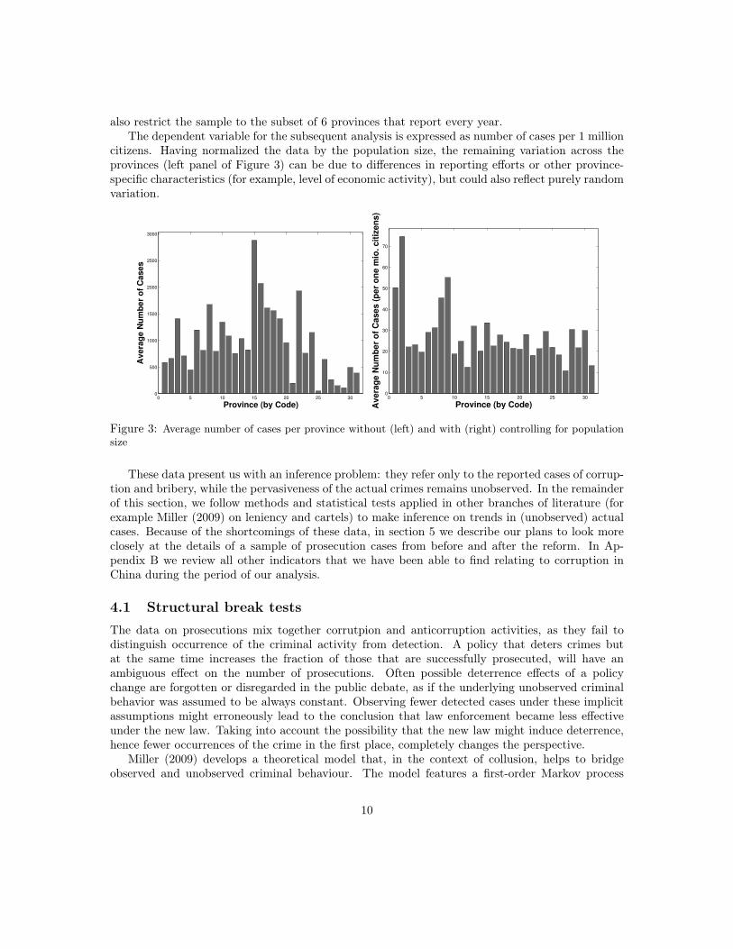
also restrict the sample to the subset of 6 provinces that report every year.The dependent variable for the subsequent analysis is expressed as number of cases per 1 million
citizens. Having normalized the data by the population size, the remaining variation across theprovinces (left panel of Figure 3) can be due to differences in reporting efforts or other province-specific characteristics (for example, level of economic activity), but could also reflect purely randomvariation.
0 5 10 15 20 25 300
500
1000
1500
2000
2500
3000
Province (by Code)
Av
era
ge
Nu
mb
er
of
Ca
se
s
0 5 10 15 20 25 300
10
20
30
40
50
60
70
Province (by Code)Avera
ge N
um
ber
of
Cases (
per
on
e m
io. cit
izen
s)
Figure 3: Average number of cases per province without (left) and with (right) controlling for populationsize
These data present us with an inference problem: they refer only to the reported cases of corrup-tion and bribery, while the pervasiveness of the actual crimes remains unobserved. In the remainderof this section, we follow methods and statistical tests applied in other branches of literature (forexample Miller (2009) on leniency and cartels) to make inference on trends in (unobserved) actualcases. Because of the shortcomings of these data, in section 5 we describe our plans to look moreclosely at the details of a sample of prosecution cases from before and after the reform. In Ap-pendix B we review all other indicators that we have been able to find relating to corruption inChina during the period of our analysis.
4.1 Structural break testsThe data on prosecutions mix together corrutpion and anticorruption activities, as they fail todistinguish occurrence of the criminal activity from detection. A policy that deters crimes butat the same time increases the fraction of those that are successfully prosecuted, will have anambiguous effect on the number of prosecutions. Often possible deterrence effects of a policychange are forgotten or disregarded in the public debate, as if the underlying unobserved criminalbehavior was assumed to be always constant. Observing fewer detected cases under these implicitassumptions might erroneously lead to the conclusion that law enforcement became less effectiveunder the new law. Taking into account the possibility that the new law might induce deterrence,hence fewer occurrences of the crime in the first place, completely changes the perspective.
Miller (2009) develops a theoretical model that, in the context of collusion, helps to bridgeobserved and unobserved criminal behaviour. The model features a first-order Markov process
10

governing the occurrence of criminal activity (cartel formation, in this case) and derives predictionsfor how changes in the rate of occurrence and the rate of detection affect the time series of detection.This is then applied to test the effect of the introduction of leniency on cartel formation and detectionrates.
Similarly to collusive behavior leading to cartel formation, bribery is also based on trust betweenthe corrupt partners. And leniency similarly may undermine this trust Bigoni et al. (2015) leadingto deterrence effects. We exploit this similarity in the two types of criminal activity to adapt thetheoretical results and empirical tests developed by Miller (2009) to the case of the anti-briberyreforms. While cartels are long-term agreements, though, we can think of bribe exchanges asone-shot interactions.
The main results from Miller’s theoretical model are summarized as follows:RESULT 1: The immediate increase in the number of prosecutions after a reform is sufficient
to establish a corresponding increase in the detection rate.RESULT 2: The subsequent readjustment of the number of prosecutions below initial levels is
sufficient to establish a decrease in the underlying criminal activity (deterrence effect).Based on this, Miller (2009) expects a peak in discoveries after the reform due to defection of
existing cartels’ members followed by a slump, revealing less cartel formation. Given the instanta-neous nature of bribery interactions, we should not expect a separate detection effect of the samekind. On the other hand, the 1997 reform is retroactive, implying that leniency becomes availablealso for birbe-exchanges that have happened before 1997. This could potentially still lead to a peakin discoveries immediately after the reform.
The bar graph in Figure 4, showing the number of cases per 1 million citizens from 1988 until2010, yields some first insights. The average is relatively high in the first ten years of data andexhibits some time variation, before it experiences a major drop in the year 1998, coinciding withthe implementation of the reform in 1997. The average levels off in this low state in the subsequentyears.
1990 1995 2000 2005 20100
10
20
30
40
50
Year
Nu
mb
er
of
Ca
se
s (
pe
r o
ne
mil
lio
n c
itiz
en
s)
Figure 4: Number of cases over time
The box plots in Figure 5 group together observations from before and after the reform, illus-trating a difference-in-means test. The left panel uses only the province-level data. Both the median
11

- indicated by the red line - and the variance - indicated by the edges of the box, the 25th and75th percentile - are considerably lower after the reform. In line with this graphical observation,the two-sample t-test of equal means rejects the null hypothesis of equal means (and equal butunknown variances) at any common significance level.
Figure 5: Box Plot - Average number of cases before and after the reform: province-level (left) andnational-level data (right)
Since the province-level data has less observations after the reform, it seems worthwhile to usethe available national data for the post-treatment period as a robustness check. Note that theabsolute number of reported cases on the national level is weighed by the national population sizeto obtain a measure comparable with the Province-level data. The box plot in the right panelof Figure 5 yields similar results. The two-sample t-test of equal means again rejects the nullhypothesis at any common significance level.
After these first graphical observations and mean tests, we now turn to regression analysis toquantify the effect of the reform.
Figure 6 plots the dependent variable, the number of cases per one million citizens (includingin red national-level data where available).
In Column (1) of Table 4, we regress the dependent variable only on the reform dummy, whichtakes the value one for the years after 1997 and zero otherwise. The legal reform resulted in 23.66less cases per one million citizens, corresponding to a 23.66
37.95 · 100% = 62.3% decrease.In order to take into account potential trends over time, the model is augmented in the other
Columns to include polynomials of different orders in two separate time trends. The term TIME1equals one in the first period (year 1988), two in the second period, and so on. The variable TIME2equals one in the first period following the reform (year 1998), two in the next period, and soon. The coefficient on the reform dummy, which measures the treatment effect, remains close to30% and statistically significant in all but one case: Column (4), which includes a second orderpolynomial in both TIME1 and TIME2. This is probably due to the neat fit of the polynomial,as illustrated in the bottom-left panel of Figure 10 in Appendix A.17 As one would expect whenlooking at Figure 6, using the national-level data for the post-reform period yields almost identicalresults (see Appendix A).
17The inclusion of other combinations and higher polynomial orders was also tested. The treatment effect remainsstatistically significant with values in the same range.
12
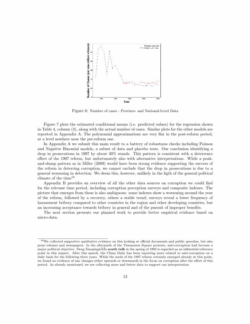
Figure 6: Number of cases - Province- and National-Level Data
Figure 7 plots the estimated conditional means (i.e. predicted values) for the regression shownin Table 4, column (3), along with the actual number of cases. Similar plots for the other models arereported in Appendix A. The polynomial approximations are very flat in the post-reform period,at a level nowhere near the pre-reform one.
In Appendix A we submit this main result to a battery of robustness checks including Poissonand Negative Binomial models, a subset of data and placebo tests. Our conclusion identifying adrop in prosecutions in 1997 by about 30% stands. This pattern is consistent with a deterrenceeffect of the 1997 reform, but unfortunately also with alternative interpretations. While a peak-and-slump pattern as in Miller (2009) would have been strong evidence supporting the success ofthe reform in deterring corruption, we cannot exclude that the drop in prosecutions is due to ageneral worsening in detection. We deem this, however, unlikely in the ligth of the general politicalclimate of the time18
Appendix B provides an overview of all the other data sources on corruption we could findfor the relevant time period, including corruption perception surveys and composite indexes. Thepicture that emerges from these is also ambiguous: some indexes show a worsening around the yearof the reform, followed by a recovery, others a stable trend; surveys reveal a lower frequency ofharassment bribery compared to other countries in the region and other developing countries, butan increasing acceptance towards bribery in general and of the pursuit of improper benefits.
The next section presents our planned work to provide better empirical evidence based onmicro-data.
18We collected supportive qualitative evidence on this looking at official documents and public speeches, but alsopress releases and newspapers. In the aftermath of the Tienanmen Square protests, anti-corruption had become amajor political objective. Deng XiaopingâĂŹs south talk in the spring of 1992 is regarded as an influential referencepoint in this respect. After this speech, the China Daily has been reporting news related to anti-corruption on adaily basis for the following three years. While the seeds of the 1997 reform certainly emerged already at this point,we found no evidence of any changes either upwards or downwards in the focus on corruption after the effort of thisperiod. As already mentioned, we are collecting more and better data to support our interpretation.
13

Table 4: OLS Regression Results
Dependent variable: Number of cases (Prosecutions for corruption and bribery)
(1) (2) (3) (4) (5)
Legal Reform DummyREFORM -23.66*** -13.66** -14.53*** -3.64 -11.87***
(4.31) (6.74) (4.77) (4.05) (3.72)
Polynomials in timeTIME1 None 2nd order 1st order 2nd order 3rd orderTIME2 None None 1st order 2nd order 3rd order
Constant 37.95*** 47.37*** 47.63*** 29.88** 5.96(4.33) (13.39) (10.62) (11.17) (16.28)
Observations 23 23 23 23 23DF 21 19 19 17 15Adj R2 0.63 0.64 0.66 0.71 0.74LL -82.20 -80.71 -80.30 -77.16 -74.33F-Statistic 38.8 14.20 15.00 11.60 9.96Notes: Heteroscedasticity and autocorrelation consistent (HAC) estimates, robust standard errors in parentheses.
TIME1 is a time trend for the whole period. TIME2 is a time trend starting after the reform.*, **, *** Significant at the 10%, 5%, and 1% level, respectively.
10
20
30
40
1990 1995 2000 2005 2010Year
Pop
ulat
ion-
adju
sted
num
ber
ofca
ses
Act
uala
ndes
tim
ated
-O
LS
Figure 7: Test for structural break – Model (3)
14

5 Case-files AnalysisAs discussed above, the data on prosecutions are subject to several limitations, both theoreticaland practical. Starting with the latter, our panel of regional reports is severely unbalanced, whilethe national ones only cover the post-reform period. Moreover, the data do not distinguish briberyfrom other corruption offences such as embezzlement, nor giving versus taking of bribes. Althougha previous case analysis study (Guo, 2008) found that 82-93% of all corruption cases (between 1978and 2005) were about bribery, and that only 4-9% of cases were against bribe-givers only, we cannotobserve using these data, what part of the drop in cases is simply due to a change in composition.In an extreme case, it could be that prosecutions against bribe-givers are not carried out anymorefor extortionary bribery cases, since they are not considered guilty any longer, explaining the dropin our aggregate statistic even if the number of cases agaisnt bribe-takers is unchanged.
Another more general limitation of prosecution data is that they do not disentangle deterrencefrom detection, or criminal activity from prosecution efforts: a policy that deters crimes but at thesame time increases the fraction of those that are successfully prosecuted will have an ambiguouseffect on the number of prosecutions. For this reason, we analyze here more in depth a stratifiedrandom sample of prosecution cases between 1986 and 2010. Given that we sample a given numberof cases, determined by power and budget considerations, in this part of the analysis we cannotgain any insight about the incidence of bribery in general. We can instead observe the impact ofthe legislative reform on specific details of the corrupt behavior, most notably whether it involvesillegittimate benefit or not, the size of the bribe and the favor exchanged, and so on, and themechanisms through which this behavior occurs or is deterred. In particular we want to distinguishbetween extortionary (harassment) bribes and bribes for illicit benefit. Moreover we want to shedlight on whether and how leniency and asymmetric punishment are applied in practice.
The outcomes that we look at are specified in a pre-analysis plan (Perrotta Berlin and Spagnolo,2015). Subsequently, in September 2015, we collected a pilot – a small random sample of case files– in order to learn more about what information is available in the case files. Here we describe ourmain outcomes of interest and hypotheses.
• Relative incidence of report by the bribe-giver. Ideally we would want to know whetherthe case was initiated by a spontaneous report. After the introduction of asymmetric pun-ishment and leniency, we should in general expect a higher frequency of cases in which thebribe-givers come forth and report the crime to the authorities in the short run. Although inpractice this will depend on the severity of sanctions and the actual likelihood of obtainingleniency, in equilibrium this effect should disappear, due to deterrence. Unfortunately theinformation on how the case was initiated is not available in the case files. There is howeversome indication of whether the defendant volunteered information if leniency was awarded.
• Relative incidence of harassment bribes in the total. Looking at the prosecutiondocuments we can first of all form a better idea of whether the presence of improper benefitis actually considered in practice, and so whether harassment bribes are effectively set apartand subject to a different discipline (in particular, the exemption from punishment for thegiver). Further, if this is the case, we can observe whether the 1997 reform led to a changein this respect, and hence on the frequency of harassment bribes relative to other types ofbribery among the cases detected.
• Size of the bribe, size of the return, income or status of the bribe-giver (and thebribe-taker) If the reform, through the introduction of leniency and asymmetric punishment,
15

makes detection easier because of the incentives provided to the bribe-giver, this amounts toan increase in the expected fine for the bribe-taker (even though the actual sanctions decrease).We expect this to lead to an increase of bribe size for distortionary bribes: the threshold toundertake corrupt behavior is now raised, hence individuals will only exchange bribes if thereturns from this corrupt agreement are higher. The picture is different though for harassmentbribes, when the bribe-giver is not expected to give back the gain. In this case incentives toreport increase with the size of the bribe, so the larger bribes will be deterred to a largerextent.
5.1 Power analysisThe aim of this exercise is to determine the minimum sample size needed to be able to observe thetrue impact of the reform. As a reminder, “[. . . ] the power of a statistical test is the probabilitythat it correctly rejects the null hypothesis. [. . . ] the power of a study depends on sample size,measurement variance, the number of comparisons being performed, and the size of the effects beingstudied." (Gelman and Carlin, 2014)
The main challenge in our case is to specify the expected effect size, given that there is nocomparable empirical work done in this area19. The optimal sample size can be computed usingoptimal design20, an algorithm that requires as input the standardized effect size, which in turnrequires an estimate of the mean and variation of the outcome(s) in the two groups. We offer herecalculations corresponding to ranges of values, going through the outcome variables, discussingwhat is reasonable to expect in terms of effect on each of them in turns.
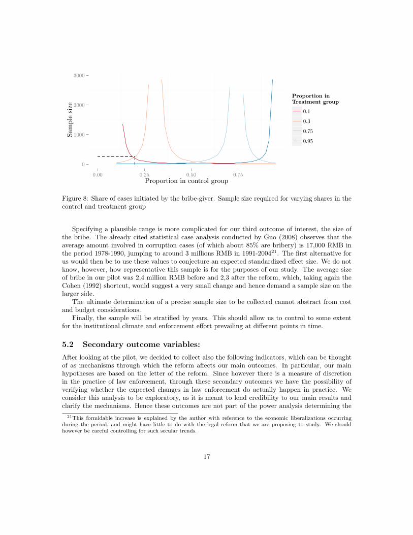
Our first outcome is a proportion, the share of cases discovered through a report by the bribe-giver, which makes it easier to specify a reasonable expected value. Starting from a desired sig-nificance level of 0.05 and power of 0.8, Figure 8 below plots the sample size as a function of theproportion (of reporting bribe-givers) in the control group, i.e. before the reform. The differentcurves correspond to different sizes of the change in this proportion after the reform. To give anexample, if we observe that the proportion of cases initiated by the bribe-giver is 19% and weexpect an increase in it by 60% after the reform (roughly corresponding to the impact estimated byMiller), we would need about 120 observations in order to correctly reject a false null hypothesis.To identify a (still big but) smaller increase by 40%, if the original proportion had been 21%, therequired sample jumps already to 483, and a 20% increase, starting from 25%, would require morethan 1800 observations.
The second outcome is also a proportion, the share of harassment bribes in the total. However,we have very little to go by in terms of expected proportions and effect sizes. There is no distinctionon this dimension in previous work, and unfortunately even in our pilot there was no instance ofharassment bribes either before or after the reform. Another alternative is represented by a moregeneral approach: a shortcut when data on mean and standard deviation of the outcomes are notavailable is to directly specify the effect size one wishes to detect in multiples of the standarddeviation of the outcome. Cohen (1992) proposes that an effect of 0.2 standard deviation is “small”,0.5 is “medium” and 0.8 is “large”. The sample size required to observe such effects, with the samesignificance and power as above, is 392, 63 and 25 respectively.
19The alternative would be to specify the minimum size of effect that we will be able to identify given the budget atour disposal. This in turn requires estimates of the factors determining the cost, namely how accessible prosecutiondocuments are, how they look like and consequently how long time it will take to process them and extract therelevant information.
20See Raudenbush et al. (2005).
16
0
1000
2000
3000
0.00 0.25 0.50 0.75Proportion in control group
Sam
ple
size
Proportion inTreatment group
0.1
0.3
0.75
0.95
Figure 8: Share of cases initiated by the bribe-giver. Sample size required for varying shares in thecontrol and treatment group
Specifying a plausible range is more complicated for our third outcome of interest, the size ofthe bribe. The already cited statistical case analysis conducted by Guo (2008) observes that theaverage amount involved in corruption cases (of which about 85% are bribery) is 17,000 RMB inthe period 1978-1990, jumping to around 3 millions RMB in 1991-200421. The first alternative forus would then be to use these values to conjecture an expected standardized effect size. We do notknow, however, how representative this sample is for the purposes of our study. The average sizeof bribe in our pilot was 2,4 million RMB before and 2,3 after the reform, which, taking again theCohen (1992) shortcut, would suggest a very small change and hence demand a sample size on thelarger side.
The ultimate determination of a precise sample size to be collected cannot abstract from costand budget considerations.
Finally, the sample will be stratified by years. This should allow us to control to some extentfor the institutional climate and enforcement effort prevailing at different points in time.
5.2 Secondary outcome variables:After looking at the pilot, we decided to collect also the following indicators, which can be thoughtof as mechanisms through which the reform affects our main outcomes. In particular, our mainhypotheses are based on the letter of the reform. Since however there is a measure of discretionin the practice of law enforcement, through these secondary outcomes we have the possibility ofverifying whether the expected changes in law enforcement do actually happen in practice. Weconsider this analysis to be exploratory, as it is meant to lend credibility to our main results andclarify the mechanisms. Hence these outcomes are not part of the power analysis determining the
21This formidable increase is explained by the author with reference to the economic liberalizations occurringduring the period, and might have little to do with the legal reform that we are proposing to study. We shouldhowever be careful controlling for such secular trends.
17

size of the sample.
• Actual likelihood of obtaining leniency. Leniency is not automatic in the text of thelaw. Since it is administered at the discretion of the judicial authority, it can be informativeto investigate how often it is accorded in practice. This might also highlight differences inattitudes between different courts, which might be exploited at a later stage.
• Actual sanctions imposed. Similarly to the previous point, sanctions are specified in thelegal text in form of ranges (ex. not less than 2 and up to 5 years imprisonement), andimply discretion for the judicial authority. It is hence interesting to verify how severe are thesanctions administered in practice. Again, this might also highlight differences in attitudesbetween different courts, which might be exploited at a later stage.
• Latency. The analysis of cases allows to some extent to distinguish the time of detectionfrom the time when the corrupt exchange took place. This gives a clearer picture of the timetrends in criminal activity as separate from discovery.
• Bureaucrat characteristics. Who becomes a bureaucrat after corruption has been mademore difficult? Is there selection into this career? We plan to collect as many personalcharacteristics of the corrupt bureaucrats from the case files as available.
6 ConclusionsThis paper provides the first empirical assessment of the effectiveness of leniency and asymmetricpunisjment as a policy tool against corrutpion. Leniency has been used before to undermine theinternal trust between partners in crime in other law enforcement areas, and this mechanism hasbeen studied theoretically in the context of corrutpion, but never evaluated empirically. Part ofthe reason lies in the difficulty to obtain good data on corrutpion. We cannot solve completelythe issue of data quality, as we also rely on official reports of counts of corruption cases. Howeverwe go a step further by collecting and analyzing microdata from a stratified randomized sampleof these cases. Whereas the aggregated data clearly show that something happened to corruptioncases in China in connection with the 1997 Criminal Law reform, and that the observed effects areconsistent with an increase in deterrence, without the microdata we wouldn’t be confident in thisinterpretation. Through the analysis of the sample we can instead isolate at a higher level of detailthe changes in criminal behavior, reporting behavior and prosecution activity and link them to thedetails of the legal reform to highlight the mechanisms at work. Overall we believe this to be asignificant contribution to our understanding of how to best taylor policy to fight corrutpion.
A further contribution of this paper is the focus on China. This country is home to a sixth ofhumanity, and currently undergoing a massive crack down on corruption. Whatever we can learnabout the effectiveness of anti-corrutpion policies is likely to have considerable welfare effects.
ReferencesAbbink, K., U. Dasgupta, L. Gangadharan, and T. Jain (2014). Letting the briber go free: An
experiment on mitigating harassment bribes. Journal of Public Economics 111, 17–28.
18
Apesteguia, J., M. Dufwenberg, and R. Selten (2007). Blowing the whistle. Economic Theory 31 (1),143–166.
Aubert, C., P. Rey, and W. E. Kovacic (2006). The impact of leniency and whistle-blowing programson cartels. International Journal of Industrial Organization 24 (6), 1241–1266.
AUCL (1993). Anti unfair competition law of the people’s republic of china. http://www.lawinfochina.com/Display.aspx?lib=law&Cgid=6359. Accessed: 2015-05-20.
Basu, K. (2011). Why, for a class of bribes, the act of giving a bribe should be treated as legal.Technical Report 172011, Ministry of Finance, Government of India.
Basu, K., K. Basu, and T. Cordella (2014). Asymmetric punishment as an instrument of corruptioncontrol. World Bank Policy Research Working Paper (6933).
Bigoni, M., S.-O. Fridolfsson, C. Le Coq, and G. Spagnolo (2012). Fines, leniency, and rewards inantitrust. The RAND Journal of Economics 43 (2), 368–390.
Bigoni, M., S.-O. Fridolfsson, C. Le Coq, and G. Spagnolo (2015). Trust, leniency, and deterrence.Journal of Law, Economics, and Organization.
Brenner, S. (2009). An empirical study of the european corporate leniency program. InternationalJournal of Industrial Organization 27 (6), 639–645.
Buccirossi, P. and G. Spagnolo (2006). Leniency policies and illegal transactions. Journal of PublicEconomics 90 (6), 1281–1297.
CCPCC (2014). CCP Central Committee Decision Concerning Several Major Issues In Com-prehensively Advancing Governance According To Law. http://chinalawtranslate.com/en/fourth-plenum-decision/. Accessed: 2015-05-20.
CCTV (2014). CCTV NewsContent. http://220.181.168.86/NewJsp/news.jsp?fileId=286007.Accessed: 2015-05-20.
Chen, Z. and P. Rey (2013). On the design of leniency programs. Journal of Law and Eco-nomics 56 (4), 917–957.
ChinaDaily (2015). China to speed up drafting anti-corruption law. http://www.chinadaily.com.cn/china/2015twosession/2015-03/08/content_19751223.htm. Accessed: 2015-05-20.
CL (1997). Criminal law of the people’s republic of china in database of laws and regulations. http://www.npc.gov.cn/englishnpc/Law/2007-12/13/content_1384075.htm. Accessed: 2015-05-20.
Cohen, J. (1992). A power primer. Psychological bulletin 112 (1), 155.
Cohen, J. A., T. A. Gelatt, and F. M. T. b. Li (1982). The criminal law of the people’s republicof china. J. Crim. L. & Criminology 73, 138. http://scholarlycommons.law.northwestern.edu/cgi/viewcontent.cgi?article=6292&context=jclc.
Dreze, J. (2011). The bribing game. Indian Express 23.
19

Dufwenberg, M. and G. Spagnolo (2015). Legalizing bribe giving. Economic Inquiry .
Engel, C., S. J. Goerg, and G. Yu (2012). Symmetric vs. asymmetric punishment regimes forbribery. SSRN Working Paper Series.
Gelman, A. and J. Carlin (2014). Beyond power calculations assessing type s (sign) and type m(magnitude) errors. Perspectives on Psychological Science 9 (6), 641–651.
Gintel, S. R. (2013). Fighting transnational bribery: China’s gradual approach. Wisconsin Inter-national Law Journal 31 (1).
Guo, Y. (2008). Corruption in transitional china: An empirical analysis. China Quarterly 194, 349.
Harrington, J. E. (2008). Optimal corporate leniency programs. The Journal of Industrial Eco-nomics 56 (2), 215–246.
Harrington, J. E. (2013). Corporate leniency programs when firms have private information: Thepush of prosecution and the pull of pre-emption. The Journal of Industrial Economics 61 (1),1–27.
Harrington, J. E. and M.-H. Chang (2009). Modeling the birth and death of cartels with anapplication to evaluating competition policy. Journal of the European Economic Association 7 (6),1400–1435.
Hinloopen, J. and A. R. Soetevent (2008). Laboratory evidence on the effectiveness of corporateleniency programs. The RAND Journal of Economics 39 (2), 607–616.
Kaufmann, D., A. Kraay, and M. Mastruzzi (2009). Governance matters VIII: aggregate andindividual governance indicators, 1996-2008. World bank policy research working paper (4978).
Lambsdorff, J. and M. Nell (2007). Fighting corruption with asymmetric penalties and leniency.Technical report, University of Goettingen, Department of Economics.
Li, X. (2012). Guest post: bribery and the limits of game theory –the lessons from China. http://blogs.ft.com/beyond-brics/2012/05/01/guest-post-bribery-and-the-limits-of-game-theory-the-lessons-from-china/. Ac-cessed: 2015-05-20.
Miller, N. H. (2009). Strategic leniency and cartel enforcement. The American Economic Review ,750–768.
Motta, M. and M. Polo (2003). Leniency programs and cartel prosecution. International journalof industrial organization 21 (3), 347–379.
Oak, M. (2015). Legalization of bribe giving when bribe type is endogenous. Journal of PublicEconomic Theory .
Perrotta Berlin, M. and G. Spagnolo (2015). Pre-analysis plan for the impact of the introductionof leniency on bribery prosecutions in china. AEA RCT Registry . Published: 2015-07-17.
Raudenbush, S., J. Spybrook, X. Liu, and R. Congdon (2005). Optimal design for longitudinal andmulti-level research. Ann Arbor, MI: William T. Grant Foundation.
20

SCNPC (1988a). Supplementary provisions of the standing committee of the national people’scongress concerning the punishment of the crimes of embezzlement and bribery. https://aplf.com.au/article/prof-mingkai-zhang?language=eng. Accessed: 2015-05-20.
SCNPC (1988b). Supplementary provisions of the standing committee of the national people’scongress concerning the punishment of the crimes of embezzlement and bribery. http://www.npc.gov.cn/wxzl/gongbao/1988-01/21/content_1481041.htm. Accessed: 2015-05-20.
Spagnolo, G. (2000). Self-defeating antitrust laws: how leniency programs solve bertrand’s paradoxand enforce collusion in auctions.
Spagnolo, G. (2004). Divide et impera: Optimal leniency programs.
Spagnolo, G. (2008). Leniency and whistleblowers in antitrust. In P. Buccirossi (Ed.), Handbook ofAntitrust Economics. M.I.T. Press.
Tanzhihua, S. (2011). Research on “illegitimate benefit” in the guilty of offering bribes. Journal ofLaw Application (12), 59–62. http://oversea.cnki.net/kcms/detail/detail.aspx?dbCode=cjfd&QueryID=28&CurRec=14&filename=FLSY201112016&dbname=CJFD2011.
Wu, K. and K. Abbink (2013). Reward self-reporting to deter corruption: An experiment onmitigating collusive bribery. Technical report, Monash University, Department of Economics.
Appendices
A Robustness checksA.1 OLS models
As a first robustness check, we estimate the same models as in Section 4.1 on the subset of 6provinces which have a report for all the 23 years of the sample. Figure 9 shows that this makesresuts even stronger. Figures 10 and 11 report a visualization of the other models estimated inTable 4, which fit different order of polynomials in the time trends.
21

10
20
30
1990 1995 2000 2005 2010Year
Pop
ulat
ion-
adju
sted
num
ber
ofca
ses
Act
uala
ndes
tim
ated
-O
LS
Figure 9: Test for structural break in a subset of provinces
10
20
30
40
1990 1995 2000 2005 2010
Model ( 1 )
10
20
30
40
1990 1995 2000 2005 2010
Model ( 2 )
10
20
30
40
1990 1995 2000 2005 2010
Model ( 4 )
10
20
30
40
1990 1995 2000 2005 2010
Model ( 5 )
Figure 10: Test for structural break – other polynomials
22

10
20
30
1990 1995 2000 2005 2010
Model ( 1 )
10
20
30
1990 1995 2000 2005 2010
Model ( 2 )
10
20
30
1990 1995 2000 2005 2010
Model ( 4 )
10
20
30
40
1990 1995 2000 2005 2010
Model ( 5 )
Figure 11: Test for structural break – subset of non-missing provinces
A.2 Poisson regression
The linear regression model rests on assumptions that can be at odds with this particular type ofdata. The dependent variable is assumed to be continuous, normally distributed (hence symmetricaround the mean), and linearly related to the independent variables (McClendon, 1994). Crimedata rarely adhere to these assumptions. Most crime incidents are distributed as rare event counts.In other words, smaller values are much more common across spatial units than larger values, withzero often being the most commonly observed value. Such a distribution violates the aforemen-tioned assumptions of OLS regression. Although these considerations are attenuated through theaggregation and averaging of the data (remember that the dependent variable is the number ofcases per one million citizens), it is worthwhile to compare the OLS results with regression mod-els that are designed to analyze count data, namely the Poisson and negative binomial regressionmodels. The Poisson regression model is often used to model count data and contingency tables.The response variable is assumed to follow a Poisson distribution, and the logarithm of its expectedvalue can be modeled by a linear combination of unknown parameters.
Table 5 reports the results of five Poisson models corresponding to the linear models used in4. Note that the reported coefficients have to be converted in order to be comparable to the OLScoefficients. The estimated number of cases λ̂ in model (1) before the reform can be calculatedas λ̂ = exp(β̂0) = exp(3.64) = 38.09. After the reform, when the treatment dummy takes thevalue one, the estimated number of cases is λ̂ = exp(β̂0 + β̂1 · 1) = exp(3.64− 0.98) = 14.30. Thisresult is very similar to the model (1) in the OLS case, a 62.4% decrease. The other estimates canbe calculated in a similar fashion. Take for instance model (2): in the year 1997, the estimate isλ̂ = exp(β̂0 + β̂2 · 10 + β̂3 · 102) = exp(3.87− 0.05 · 10 + 0.000929 · 100) = exp(3.46) = 31.81, where
23

Table 5: Poisson and Negative Binomial models
Dependent variable: Number of cases (Prosecutions for corruption and bribery)
(1) (2) (3) (4) (5)
Legal Reform DummyREFORM -0.98*** -0.64*** -0.67*** -0.26 -0.56
(0.09) (0.18) (0.18) (0.29) (0.43)
Polynomials in timeTIME1 None 2nd order 1st order 2nd order 3rd orderTIME2 None None 1st order 2nd order 3rd order
Constant 3.64*** 3.87*** 3.88*** 3.39*** 2.79***(0.05) (0.12) (0.11) (0.20) (0.34)
Observations 23 23 23 23 23DF 21 19 19 17 15Notes: Standard errors in parentheses.
TIME1 is a time trend for the whole period. TIME2 is a time trend starting after the reform.*, **, *** Significant at the 10%, 5%, and 1% level, respectively.
β̂2 and β̂3 are the coefficients for the second order polynomial in TIME1. In the year 1998, theestimate amounts to λ̂ = exp(β̂0 + β̂1 + β̂2 · 10 + β̂3 · 112) = exp(3.87− 0.64− 0.05 · 11 + 0.000929 ·121) = exp(2.79) = 16.28. More generally, OLS and Poisson regressions yield very similar results.However, the reform coefficient loses statistical significance in model (4) and (5) and for higherorder polynomials (not reported) when using the Poisson model. The similarity in the results isnot surprising when considering that the normal distribution is a good approximation to a Poissondistribution for data with a mean above (roughly) 30. The linear model assumes that the valuesare normally distributed around the expected value and can take any real value. Hence, when themean is large enough, i.e. negative values are highly unlikely, and the variance is in a similar range,the OLS approximates the Poisson regression estimates quite well.
One drawback of the Poisson regression is the inherent assumption of equal mean and variance.Yet, we saw that the data exhibits different degrees of variation, especially when comparing thedependent variable before and after the reform. To handle overdispersed count variables, thenegative binomial distribution is often used, since it allows for variance greater than the mean,making it suitable for count data that do not meet the assumptions of the Poisson distribution.Fitting a negative binomial model to our data delivered identical results22, except sligthly inflatedstandard errors. The pattern of significance is also unchanged, with models (1) - (3) stronglysignificant but not (4) and (5).
A.3 National data
Table 6 replicates the specification of Table 4, using the national statistics on prosecutions ratherthan the province-level ones for the period after the reform as a robustness tests. These data providean upper-bound to the actual number of prosecutions in the group of provinces that we observe forthe period before the reform, as they are supposedly including all the 31 provinces. We see that
22Results are not reported but are available upon request to the authors.
24

the decrease immediately following the reform is still significant, although smaller in size.
Table 6: OLS Regression Results - National-level data for the post-reform period
Dependent variable: Number of cases (Prosecutions for corruption and bribery)
(1) (2) (3) (4) (5)
Legal Reform DummyREFORM -21.60*** -12.99** -13.91*** -3.62 -12.11***
(4.34) (7.42) (4.77) (4.16) (4.46)
Polynomials in timeTIME1 None 2nd order 1st order 2nd order 3rd orderTIME2 None None 1st order 2nd order 3rd order
Constant 37.95*** 47.41*** 47.63*** 29.88** 5.96(4.34) (14.50) (10.49) (13.08) (17.36)
Observations 22 22 22 22 22Degrees of Freedom 20 18 18 16 14Adjusted R2 0.58 0.59 0.66 0.66 0.70Log Likelihood -79.02 -77.71 -77.22 -74.22 -71.48F-Statistic 30.00 10.90 11.70 9.18 7.92Notes: Heteroscedasticity and autocorrelation consistent (HAC) estimates, robust standard errors in parentheses.
TIME1 is a time trend for the whole period. TIME2 is a time trend starting after the reform.*, **, *** Significant at the 10%, 5%, and 1% level, respectively.
A.4 Placebo Interventions
So far we imposed to the data an exogenous breakpoint at the date of leniency introduction. Analternative approach would be to check whether alternative breakpoints - i.e. a different hypotheticaltiming of the legal reform - fit the data better. If this were the case, then it would be unlikely thatthe relationship between the reform introduction and the time series of prosecutions would be causal.If instead the fit is superior when the breakpoint is imposed at the date of the reform, then thedata provide support for our hypothesis. Recent literature suggests the Quandt-Likelihood Ratio(QLR) test for detecting structural changes of unknown timing (e.g., Hansen, 2001). The QLR testconsists of calculating Chow breakpoint tests at every observation, while ensuring that subsamplepoints are not too near the end points of the sample.
The results are shown in Figure 12. Each point on the graph in panels (a) and (b) representsthe maximized log-likelihood of a different regression specification. The x-axis is rescaled with0 for 1997, the year of the reform. Looking at panel (a), the maximized log-likelihood valueis located in 1990, when allowing for breakpoints between 1990-2008 (i.e. a symmetric window,trimming 2 observations from each end of the sample). The corresponding fitted values of theplacebo intervention with breakpoint in 1990 are illustrated in panel (c). Looking at panel (c)it becomes evident that 1990 has the highest maximized likelihood because it describes the kinkin the dependent variable around 1990. However, looking at the actual data, it is clear that thiscorresponds to the sharp increase in cases around 1990, which plausibly have very little to do withthe events in 1997. The test is looking for a global maximum, and hence we should be cautious withthe interpretation of the results and the choice of an appropriate window for possible breakpoints.
25

(a) Maximum log-likelihood 1990-2008 (b) Maximum log-likelihood 1992-2006
(c) Fitted Values with Maximizing Break-point (1990)
(d) Fitted Values with Maximizing Break-point (1996)
Figure 12: QLR test for structural change of unknown timing
In fact, the results change when a smaller window is chosen. Allowing for breakpoints between1992-2006 (again a symmetric window, this time leaving out the first and last 4 observations), thelog-likelihood is maximized in the year 1996. In particular, the maximized log-likelihood producedby the placebo intervention in 1996 is the only one greater than the one produced by the actuallegal reform in 1997. By visual inspection of the bottom panels of the figure, it is clear that thefitted values approximate the data much better in panel (d) compared to panel (c), both beforeand after the reform. The year 1990 as a breakpoint with the highest maximum log-likelihood ofthe placebo interventions might therefore just be an anomaly.
26
2.4
2.8
3.2
3.6
1995 2000 2005 2010Year
CPI
25
30
35
40
1995 2000 2005 2010 2015Year
Freedom from Corruption
Figure 13: Composite indices of corruption perceptions
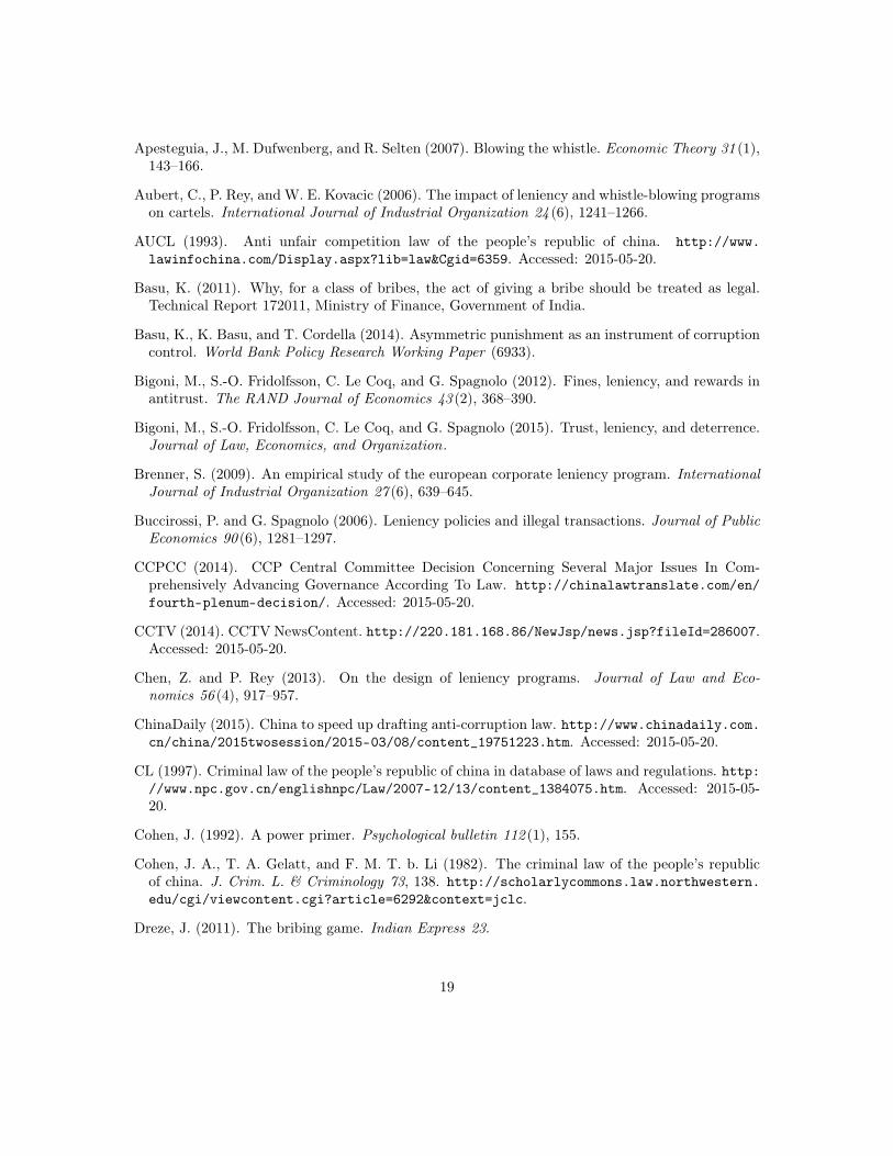
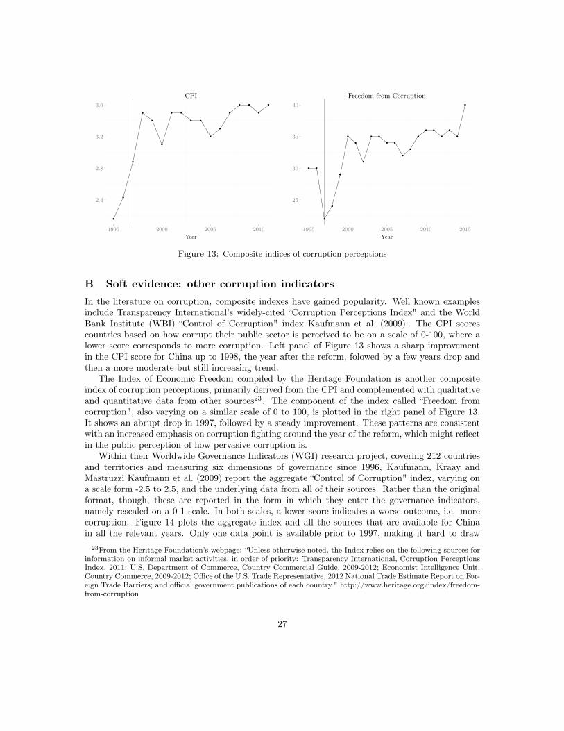
B Soft evidence: other corruption indicatorsIn the literature on corruption, composite indexes have gained popularity. Well known examplesinclude Transparency International’s widely-cited “Corruption Perceptions Index" and the WorldBank Institute (WBI) “Control of Corruption" index Kaufmann et al. (2009). The CPI scorescountries based on how corrupt their public sector is perceived to be on a scale of 0-100, where alower score corresponds to more corruption. Left panel of Figure 13 shows a sharp improvementin the CPI score for China up to 1998, the year after the reform, folowed by a few years drop andthen a more moderate but still increasing trend.
The Index of Economic Freedom compiled by the Heritage Foundation is another compositeindex of corruption perceptions, primarily derived from the CPI and complemented with qualitativeand quantitative data from other sources23. The component of the index called “Freedom fromcorruption", also varying on a similar scale of 0 to 100, is plotted in the right panel of Figure 13.It shows an abrupt drop in 1997, followed by a steady improvement. These patterns are consistentwith an increased emphasis on corruption fighting around the year of the reform, which might reflectin the public perception of how pervasive corruption is.
Within their Worldwide Governance Indicators (WGI) research project, covering 212 countriesand territories and measuring six dimensions of governance since 1996, Kaufmann, Kraay andMastruzzi Kaufmann et al. (2009) report the aggregate “Control of Corruption" index, varying ona scale form -2.5 to 2.5, and the underlying data from all of their sources. Rather than the originalformat, though, these are reported in the form in which they enter the governance indicators,namely rescaled on a 0-1 scale. In both scales, a lower score indicates a worse outcome, i.e. morecorruption. Figure 14 plots the aggregate index and all the sources that are available for Chinain all the relevant years. Only one data point is available prior to 1997, making it hard to draw
23From the Heritage Foundation’s webpage: “Unless otherwise noted, the Index relies on the following sources forinformation on informal market activities, in order of priority: Transparency International, Corruption PerceptionsIndex, 2011; U.S. Department of Commerce, Country Commercial Guide, 2009-2012; Economist Intelligence Unit,Country Commerce, 2009-2012; Office of the U.S. Trade Representative, 2012 National Trade Estimate Report on For-eign Trade Barriers; and official government publications of each country." http://www.heritage.org/index/freedom-from-corruption
27

-0.4
0.0
0.4
2000 2005 2010
Year
Inde
x
Control of Corruption
Institute for Management and DevelopmentWorld Competitiveness YearbookPolitical Economic Risk ConsultancyCorruption in Asia SurveyPolitical Risk ServicesInternational Country Risk GuideWorld Economic ForumGlobal Competitiveness Report
Figure 14: WBI Control of Corruption Index and components
any inference on the impact of the reform. In general, the aggregate index gives a rather negativeassessment of the trends in corruption, although all the components seem rather stationary.
This illustrates one of the main drawbacks of this type of composite indexes. The sources usedin constructing them can change over time. This implies that different values are likely to reflectdiffering implicit definitions of corruption, depending on what goes into them. The standardizationprocedure used to place different indicators on a common scale can also impair the ability totrack changes meaningfully over time. A final issue with the indexes that use expert sources istheir interdependence. If expert assessments display high correlations driven by the fact that theyconsult each other’s ratings - or that they all base their ratings on the same information sources -this can undermine the main premise of the aggregation methodology that averaging more sourcesproduces more accurate and reliable estimates.
We considered separately also the components of the CPI index. These were ultimately notincluded here due to either not being publicly available, not covering a sufficient number of years,or not referring specifically to bribery. For some sources, though, we were able to access the unpub-lished firm-level responses that are behind the publicly released country-level index. Surveys arerelatively well-suited for evaluating the administrative corruption, as they measure the prevalenceof corruption as experienced by users of government services. However, surveys are less effective inassessing the prevalence of corrupt transactions that occur entirely within the state, for examplewhen politicians bribe bureaucrats. The Business Environment and Enterprise Performance Sur-vey (BEEPS) and the World Economic Forum (WEF) “Executive Opinion Survey" are the mostresearch-friendly surveys on corruption-related topics, as they are systematic and comparable acrosscountries and years, have broad coverage and disclose most informations about their definitions andmethodology. The BEEPS, funded by the EBRD, are focused on Eastern Europe and Central Asiaand not available for China, however, while the WEF includes China as long back as at least 199524.In the question of interest, survey respondents were asked how common it is for firms to make un-
24Note that the WEF has conducted the Executive Opinion Survey for over 30 years, but due to methodologychanges they are unwilling to provide data going further back in time than 2004.
28

documented extra payments or bribes connected with imports and exports; public utilities; annualtax payments; awarding of public contracts and licensing; and obtaining favorable judicial decisions.In all of these cases, the assessment is improving with very similar downward trends in the period2004-201325.
Another source that similarly elicits the information about what service the bribe was paid for isthe World Bank’s Enterprise Surveys, collected since 2002 from 130,000 companies in 135 countries.Unfortunately only one year is available for China. As reported in Table 7 below, according to thissource bribery incidence in 2012 is lower in China (11.6% of firms experiencing at least one bribepayment request) both compared to the East Asian and Pacific region (24.2%) and to the wholesurvey sample (17%). However, bribery associated with illegitimate benefit is more common whileextortionary bribery is less common in both comparisons (columns (2) and (3) of Table 7).
Table 7: Unjust-benefit bribes VS harassment bribes in 2012
Bribery inci-dence (percentof firms experi-encing at leastone bribe pay-ment request)
Percent of firmsexpected to givegifts to securegovernment con-tract
Percent of firmsexpected to givegifts to publicofficials “to getthings done"
China 11.6 42.2 10.7EAP 24.2 31.0 20.4All 17.0 26.4 19.6Source: World Bank Group Enterprise Surveys
Finally, the World Value Survey is another well-known source of data on opinions and attitudesaround the globe. From the WVS we focus on two variables: the share of respondents supportingthe view that it is justfiable to accept a bribe in the exercise of one’s duty; and the share ofrespondents that think it is justifiable to claim benefits to which one is not entitled. The first onecan be thought of as a proxy for how widespread the practice of bribing public officials is in general.The second can instead be related to the practice of using or at least supporting the use of briberyto obtain an illegitimate benefit.
In the left panel of Figure 15, a decreasing trend in the acceptance of passive bribery seemsto have been reverted by the legal change. Even though there are too few data poins to actuallyestablish a pre-reform decreasing trend, it is clear that the share of respondents supporting thisview increased after the reform. This is somewhat reminiscent of the critique moved to asymmetricpunishment as a depenalization of a wrong behavior, which would over time undermine the moralsense26. The left panel shows instead that the acceptance for the behavior of seeking a benefit oneis not entitled to only grew over time since 1990. In this case, the legal change did not impact thesecular trend.
25The results are not reported. The distinction between different circumstances in which a bribe payment mightoccur can be suggestive about the presence or not of illegitimate benefit, that is relevant for the application ofimpunity according to the law. However, since there is no difference in the trends, no relevant inference can bedrawn. Moreover the time horizon of these data does not cover the implementation of the reform.
26For example in Dreze (2011).
29

0.1
0.2
0.3
0.4
1990 1995 2000 2005 2010Year
Accept bribe on duty
0.2
0.4
0.6
1990 1995 2000 2005 2010Year
Claim gov benefit if not entitled
Figure 15: Share of respondents who think behavior is justifiable
30