lesson 1 grade breakdown: general information …pirun.ku.ac.th/~fengwtc/teaching/208322 mechanical...

208322 Mechanical Vibrations Lesson 1

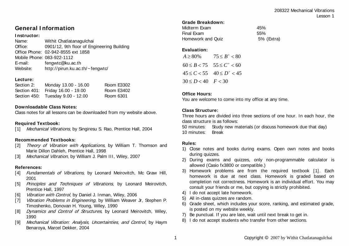
General Information Instructor: Name: Withit Chatlatanagulchai Office: 0901/12, 9th floor of Engineering Building Office Phone: 02-942-8555 ext 1858 Mobile Phone: 083-922-1112 E-mail: [email protected] Website: http://pirun.ku.ac.th/~fengwtc/ Lecture: Section 2: Monday 13.00 - 16.00 Room E3302 Section 401: Friday 16.00 - 19.00 Room E3402 Section 450: Tuesday 9.00 - 12.00 Room 6301 Downloadable Class Notes: Class notes for all lessons can be downloaded from my website above. Required Textbook: [1] Mechanical Vibrations, by Singiresu S. Rao, Prentice Hall, 2004 Recommended Textbooks: [2] Theory of Vibration with Applications, by William T. Thomson and

Marie Dillon Dahleh, Prentice Hall, 1998 [3] Mechanical Vibration, by William J. Palm III, Wiley, 2007 References: [4] Fundamentals of Vibrations, by Leonard Meirovitch, Mc Graw Hill,

2001 [5] Principles and Techniques of Vibrations, by Leonard Meirovitch,

Prentice Hall, 1997 [6] Vibration with Control, by Daniel J. Inman, Wiley, 2006 [7] Vibration Problems in Engineering, by William Weaver Jr, Stephen P.

Timoshenko, Donovan H. Young, Wiley, 1990 [8] Dynamics and Control of Structures, by Leonard Meirovitch, Wiley,

1990 [9] Mechanical Vibration: Analysis, Uncertainties, and Control, by Haym

Benaroya, Marcel Dekker, 2004

Grade Breakdown: Midterm Exam 45% Final Exam 55% Homework and Quiz 5% (Extra) Evaluation:

80% 75 8060 75 55 6045 55 40 4530 40 30

A BB CC DD F

+

+

+

≥ ≤ <

≤ < ≤ <≤ < ≤ <

≤ < < Office Hours: You are welcome to come into my office at any time. Class Structure: Three hours are divided into three sections of one hour. In each hour, the class structure is as follows: 50 minutes: Study new materials (or discuss homework due that day) 10 minutes: Break Rules: 1) Close notes and books during exams. Open own notes and books

during quizzes. 2) During exams and quizzes, only non-programmable calculator is

allowed (Casio fx3800 or compatible.) 3) Homework problems are from the required textbook [1]. Each

homework is due at next class. Homework is graded based on completion not correctness. Homework is an individual effort. You may consult your friends or me, but copying is strictly prohibited.

4) I do not accept late homework. 5) All in-class quizzes are random. 6) Grade sheet, which includes your score, ranking, and estimated grade,

is posted on my website weekly. 7) Be punctual. If you are late, wait until next break to get in. 8) I do not accept students who transfer from other sections.

1 Copyright 2007 by Withit Chatlatanagulchai


Course Schedule: Monday Tuesday Wednesday Thursday Friday Saturday Sunday

4 June (2) Lesson 1

5 June 6 June (450) Lesson 1


9 June 10 June

11 June (2) Lesson 2


14 June 15 June (401) Lesson 2 Add/Drop 1 (KU 3)

16 June 17 June




23 June 24 June




30 June 1 July

2 July (2) Lesson 5

3 July Drop 2 (No Grade W)

4 July (450) Lesson 5

5 July 6 July (401) Lesson 5

7 July 8 July

9 July (2) Lesson 6



14 July 15 July




21 July 22 July


24 July Commence-ment (No Class)




28 July Midterm Week (No Class)




1 August Midterm Week (No Class)

2 August Midterm Exam 12.00-15.00PM

3 August Midterm Week (No Class)

4 August 5 August

6 August (2) Lesson 9

7 August 8 August (450) Lesson 8


11 August 12 August

13 August Queen’s Birthday Subst. (No Class)



18 August 19 August




25 August 26 August


28 August Drop 3 (Grade W)



1 September 2 September

3 September (2) Lesson 12

4 September 5 September (450) Lesson 12











24 September Final Weeks (No Class)







1 October Final Weeks (No Class)



4 October Final Exam 13.00-16.00PM


6 October

7 October

Course Content: Contents and homework problems are based on the required textbook [1]. Lesson Contents

1 Introduction to Vibrations • Degrees of Freedom • Categories of Vibrations

Harmonic Motion • Exponential Form

Periodic Motion • Fourier Series

Vibration Terminology 2 Vibration Analysis Procedure

Vibration Model • Mechanical Elements

One Degree of Freedom, Free VibrationsSystems with Mass and Spring Natural Frequency

3 Systems with Mass, Spring, and Damper • Underdamped Case • Overdamped Case • Critically Damped Case • Logarithmic Decrement

Coulomb Damping 4 EOM 1: Newton’s Method

EOM 2: Energy Method 5 EOM 3: Equivalent System Method (Rayleigh’s Method)

EOM 4: Virtual Work Method (D’ Alembert’s Method) 6 One Degree of Freedom, Harmonically Excited Vibrations

Forced Harmonic Vibration • Frequency Response Curves

Rotating Unbalance Support Motion

7 Vibration Isolation Sharpness of Resonance Energy Dissipated by Damping Vibration-Measuring Instruments



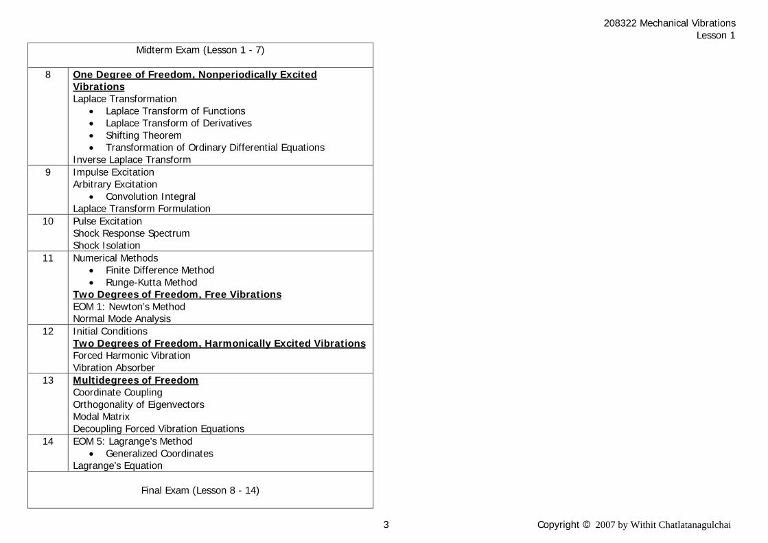
Midterm Exam (Lesson 1 - 7)

8 One Degree of Freedom, Nonperiodically Excited Vibrations Laplace Transformation

• Laplace Transform of Functions • Laplace Transform of Derivatives • Shifting Theorem • Transformation of Ordinary Differential Equations

Inverse Laplace Transform 9 Impulse Excitation

Arbitrary Excitation • Convolution Integral

Laplace Transform Formulation 10 Pulse Excitation

Shock Response Spectrum Shock Isolation

11 Numerical Methods • Finite Difference Method • Runge-Kutta Method

Two Degrees of Freedom, Free Vibrations EOM 1: Newton’s Method Normal Mode Analysis

12 Initial Conditions Two Degrees of Freedom, Harmonically Excited Vibrations Forced Harmonic Vibration Vibration Absorber

13 Multidegrees of FreedomCoordinate Coupling Orthogonality of Eigenvectors Modal Matrix Decoupling Forced Vibration Equations

14 EOM 5: Lagrange’s Method • Generalized Coordinates

Lagrange’s Equation

Final Exam (Lesson 8 - 14)



1 Introduction to Vibrations Any motion that repeats itself after an interval of time is called vibration or oscillation. Examples of vibration are

• we hear because our eardrums vibrate • we see because light waves undergo vibration • breathing is vibration of lungs • walking involves oscillatory motion of legs and hands • we speak due to the oscillation of tongue • destruction of Tacoma Narrows bridge

Figure 1: Destruction of Tacoma Narrows bridge [1].

• explosion of space shuttle Challenger

Figure 2: Explosion of Challenger [2].

A vibratory system includes mass (to store kinetic energy), spring (to store potential energy), and damper (means by which energy is gradually lost.)

1.1 Degrees of Freedom Degrees of Freedom is the minimum number of independent coordinates required to determine completely the positions of all parts of a system at any instant of time. For example,

• a free particle undergoing general motion in space has three degrees of freedom (x,y,z)

• a rigid body in space has six degrees of freedom (three components for position and three components for orientation)

• a continuous elastic body has infinite number of degrees of freedom

The coordinates necessary to describe the motion of a system constitute a set of generalized coordinates. ☻ Example 1: [3] Determine number of degrees of freedom and generalized coordinates of the following systems. a)

Solution 1 DOF, .θ



b)

Solution 3 DOF, 1 2 3, , .θ θ θ c)

Solution infinite degrees of freedom d)

Solution 2 DOF, , .x θ

e)

Solution 6 DOF, 3.1 2, , , , ,x y z θ θ θ f)

Solution 7 DOF, 1 2, , , , , , .r lx y z θ θ θ θ



1.2 Categories of Vibrations • Discrete versus Continuous Systems

Systems with a finite number of degrees of freedom are called discrete systems or lumped parameter systems. Systems with an infinite number of degrees of freedom are called continuous systems or distributed systems. Most of the time, continuous systems are approximated as discrete systems, and solutions are obtained in a simpler manner.

• Free versus Forced Vibrations Free vibration is vibration of a system, after an initial disturbance, is left to vibrate on its own without external force acting on the system. Forced vibration is vibration of a system that is subjected to an external force. The system under free vibration will vibrate at one or more of its natural frequencies. When the system is excited (forced), the system is forced to vibrate at the excitation frequency.

• Undamped versus Damped Vibrations If no energy is lost or dissipated in friction or other resistance during oscillation, the vibration is known as undamped vibration. If any energy is lost in this way, it is called damped vibration.

• Linear versus Nonlinear Vibrations A linear system obeys principle of superposition shown in Figure 3. If the system does not obey principle of superposition, the system is said to be nonlinear system and hence having nonlinear vibration.

Vibrating System

Vibrating System

Vibrating System

1u 1y

2u 2y

1 2au bu+ 1 2ay by+

Figure 3: Principle of superposition of a linear

system.

• Deterministic versus Random Vibrations Vibration that results from excitation (force or motion) that can be predicted at any given time is called deterministic vibration. If the excitation at a given time cannot be predicted, the vibration is called nondeterministic or random vibrations.

Figure 4: Deterministic and random excitations

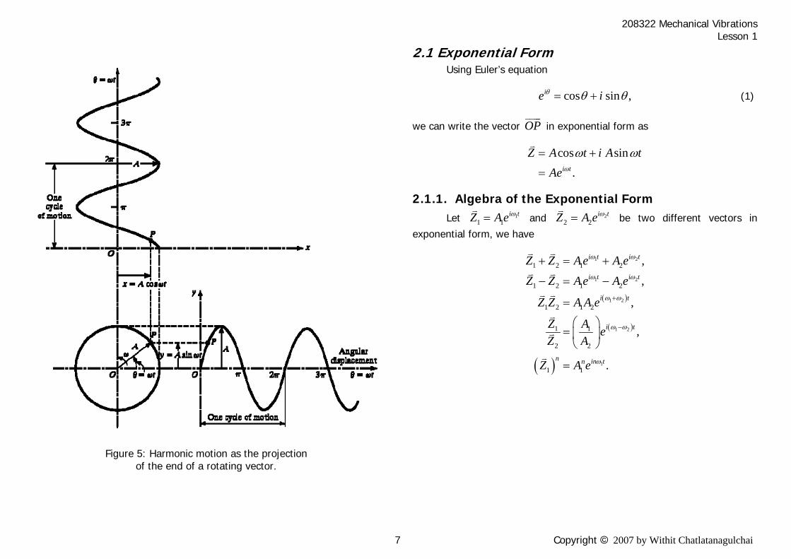
2 Harmonic Motion Harmonic motion is motion of an oscillating system that vibrates at one fixed frequency. Consider Figure 5, the harmonic motion can be represented by a vector of magnitude OP A rotating at a constant angular velocity ω . The projection of the tip of the vector OP on the vertical axis is given by

sin ,y A tω=

and the projection on the horizontal axis is given by

cos .x A tω=

If we replace the x-y plane with a complex plane where x-axis represents real axis and y-axis represents imaginary axis, we can write the vector in complex format as OP

cos sin ,Z x iy

A t i A tω ω= += +

where 1.i = −



Figure 5: Harmonic motion as the projection

of the end of a rotating vector.

2.1 Exponential Form Using Euler’s equation

cos sin ,ie iθ θ θ= + (1)

we can write the vector OP in exponential form as

cos sin.i t

Z A t i A tAe ω

ω ω= +

=

2.1.1. Algebra of the Exponential Form Let 1

1 1i tZ Ae ω= and 2

2 2i tZ A e ω= be two different vectors in

exponential form, we have

( )

( )

( )

1 2

1 2

1 2

1 2

1

1 2 1 2

1 2 1 2

1 2 1 2

1 1

2 2

1 1

,

,

,

,

.

i t i t

i t i t

i t

i t

n in tn

Z Z Ae A e

Z Z Ae A e

Z Z A A e

Z A eZ A

Z A e

ω ω

ω ω

ω ω

ω ω

ω

+

−

+ = +

− = −

=

⎛ ⎞= ⎜ ⎟⎝ ⎠

=



☻ Example 2: [3] Find the sum of the two harmonic motions ( )1 10cosx t tω= and ( ) ( )2 15cos 2 .x t tω= +



Solution Let the sum of the two harmonic motions be

( ) ( )

( )( ) ( )( )cos

cos cos sin sin .

x t A t

t A t A

ω α

ω α ω

= +

= − α (2)

Then,

( ) ( ) ( )( )

( ) (3)

( )( ) ( )( )

1 2

10cos 15cos 2

10cos 15 cos cos 2 sin sin 2

cos 10 15cos 2 sin 15sin 2 .

x t x t x t

t t

t t t

t t

ω ω

ω ω ω

ω ω

= +

= + +

= + −

= + −

Comparing (2) with (3), we have

cos 10 15cos2,A α = + (4)

and

sin 15sin 2.A α = (5)

From (4) and (5), we have

( ) ( )2 2

1

10 15cos2 15sin 2

14.148,10 15cos 2cos

14.1481.3 .

A

rad

α −

= + +

=+

=

=

Therefore, we have the sum as

( ) ( )14.148cos 1.3 .x t tω= +

2.1.2. Velocity and Acceleration of Harmonic Motion Consider a rotating vector ,i tZ Ae ω= its derivatives with respect to time are

2

2 22

,

.

i t

i t

dZ i Ae i Zdtd Z Ae Zdt

ω

ω

ω ω

ω ω

= =

= − = − (6)

The projection of i tZ Ae ω= on the horizontal axis is cosx A tω= whose derivatives are given as

( )2

2 22

sin cos ,2

cos cos .

dx A t A tdt

d x A t A tdt

πω ω ω ω

ω ω ω ω π

⎛ ⎞= − = +⎜ ⎟⎝ ⎠

= − = +

(7)

We can see from both (6) and (7) that the acceleration vector leads the velocity vector by 90 degrees, and the velocity vector leads the displacement vector by 90 degrees as shown in Figure 6.

Figure 6: Displacement, velocity, and acceleration vectors as rotating vectors.



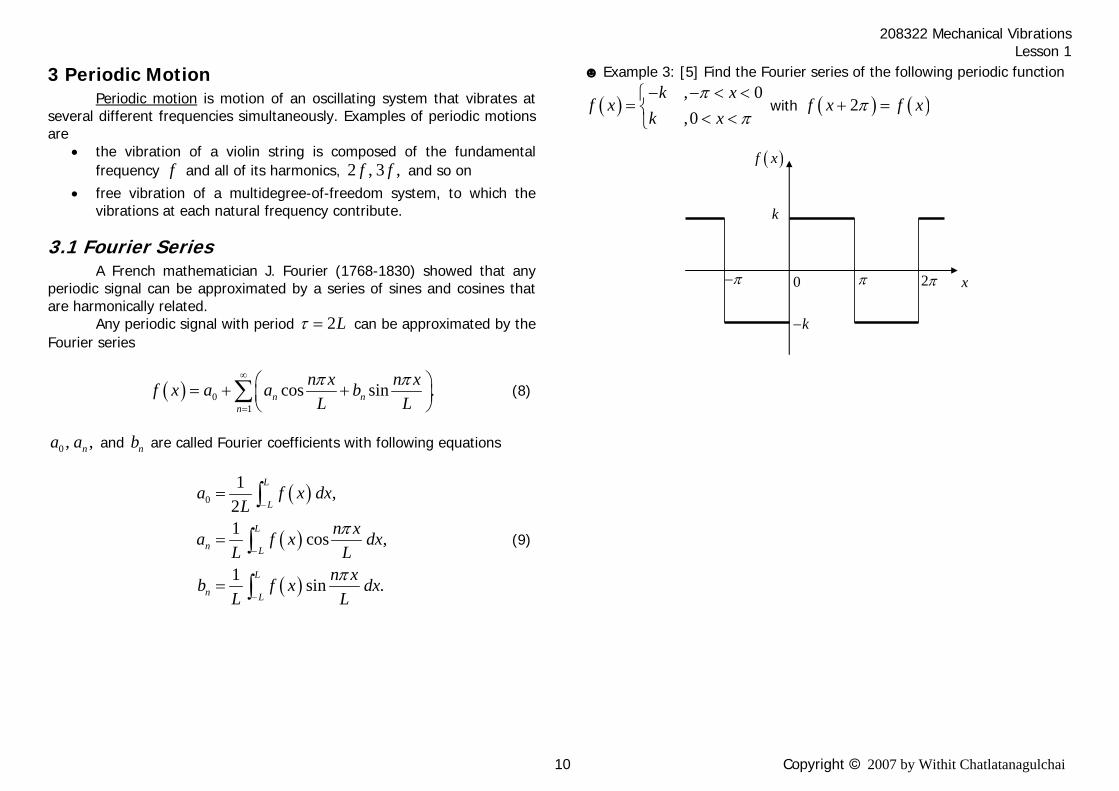
3 Periodic Motion Periodic motion is motion of an oscillating system that vibrates at several different frequencies simultaneously. Examples of periodic motions are

• the vibration of a violin string is composed of the fundamental frequency f and all of its harmonics, 2 , 3 ,f f and so on

• free vibration of a multidegree-of-freedom system, to which the vibrations at each natural frequency contribute.

3.1 Fourier Series A French mathematician J. Fourier (1768-1830) showed that any periodic signal can be approximated by a series of sines and cosines that are harmonically related. Any periodic signal with period 2Lτ = can be approximated by the Fourier series

( ) 01

cos sin .n nn

n x n xf x a a bL Lπ π∞

=

⎛ ⎞= + +⎜ ⎟ (8) ⎝ ⎠

∑

0 , ,na a and are called Fourier coefficients with following equations nb

( )

( )

( )

01 ,

21 cos ,

1 sin .

L

L

L

n L

L

n L

a f x dxL

n xa f x dxL L

n xb f x dxL L

π

π

−

−

−

=

=

=

∫

∫

∫

(9)

☻ Example 3: [5] Find the Fourier series of the following periodic function

( ), 0,0

k xf x

k xπ

π− − < <⎧

= ⎨ < <⎩ with ( ) ( )2f x f xπ+ =

( )f x

k

k−

0 π 2π xπ−



-6 -4 -2 0 2 4 6

-1

0

1

-6 -4 -2 0 2 4 6

-1

0

1

-6 -4 -2 0 2 4 6

-1

0

1

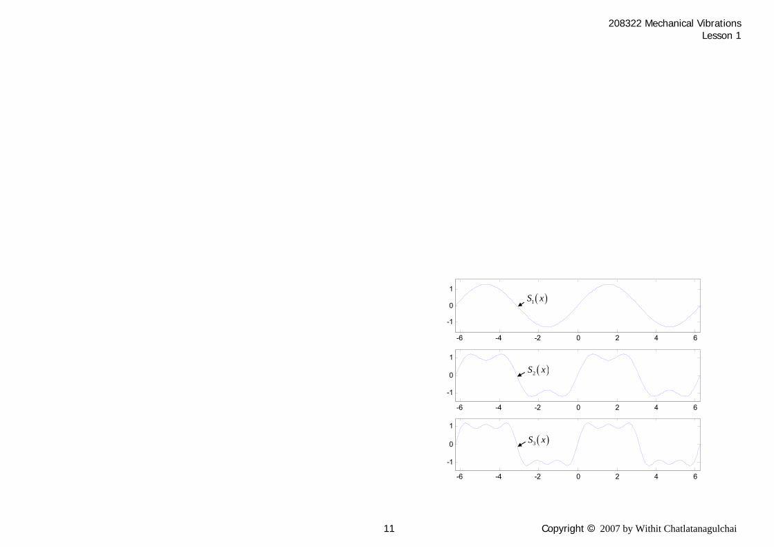
( )1S x

( )2S x

( )3S x



Solution In (8), the period is . Since the signal has period 2L 2 ,π we have

2 2 ,.

LL

ππ

==

From (9), we have

( )0

0

0

12

12

0,

a f x dx

k dx k dx

π

π

π

π

π

π

−

−

=

⎛ ⎞= − +⎜ ⎟

⎝ ⎠=

∫

∫ ∫

( )1 cos

0,

nn xa f x dx

π

ππ π−

=

=

∫π

( )

( )

( )

0

0

0

0

1 sin

1 sin sin

1 cos cos

1 cos cos

2 cos 1 .

nn xb f x dx

k nx dx k nx dx

k knx nxn n

k k k kn nn n n n

k nn

π

π

π

π

π

ππ π

π

π

π ππ

π

3.1.1. Complex Form The Fourier series can be written in complex form using the Euler’s equation (1) as follows

( )

( )

/

/

,

1 .2

in x Ln

n

L in x Ln L

f x c e

c f x e dxL

π

π

∞

=−∞

−

−

=

=

∑

∫

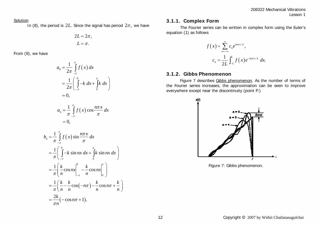
3.1.2. Gibbs Phenomenon Figure 7 describes Gibbs phenomenon. As the number of terms of the Fourier series increases, the approximation can be seen to improve everywhere except near the discontinuity (point P.)

π

π

−

−

−

=

⎛ ⎞= − +⎜ ⎟

⎝ ⎠⎛ ⎞

= −⎜ ⎟⎜ ⎟⎝ ⎠⎛ ⎞= − − − +⎜ ⎟⎝ ⎠

= − +

∫

∫ ∫

Figure 7: Gibbs phenomenon.



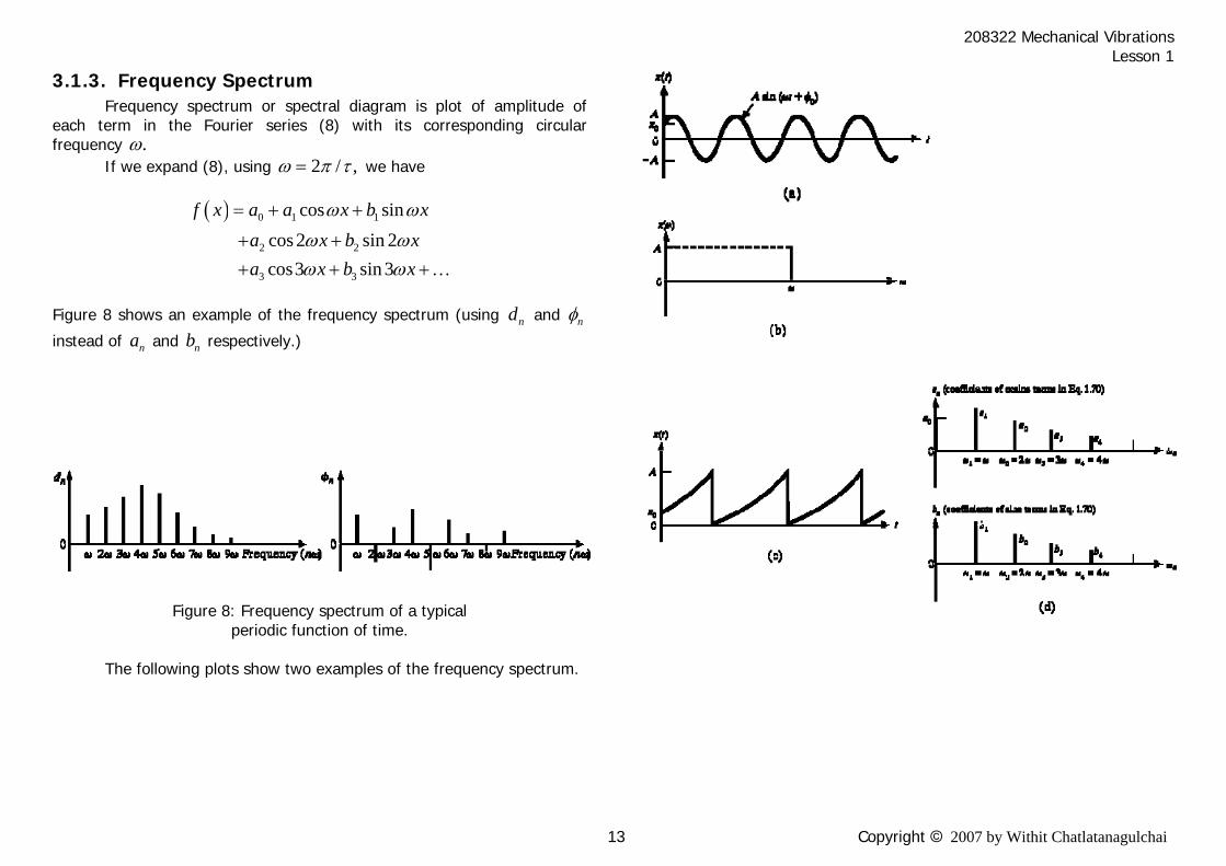
3.1.3. Frequency Spectrum Frequency spectrum or spectral diagram is plot of amplitude of each term in the Fourier series (8) with its corresponding circular frequency .ω If we expand (8), using ,2 /ω π τ= we have

( ) 0 1 1

2 2

3 3

cos sincos 2 sin 2cos3 sin 3

f x a a x b xa x b xa x b x

ω ωω ωω ω

= + +

+ ++ + +…

Figure 8 shows an example of the frequency spectrum (using and nd nφ

instead of and respectively.) na nb

Figure 8: Frequency spectrum of a typical periodic function of time.

The following plots show two examples of the frequency spectrum.



4 Vibration Terminology Certain terminologies used in vibration analysis are as follows. Peak Value generally means the maximum value of a vibrating body. Amplitude is the maximum displacement of a vibrating body from its equilibrium position. Average Value or Mean Value indicates a steady or static value. It can be found by the time integral

( )0

1lim .T

Tx x t dt

T→∞= ∫

If the signal ( )x t is periodic, the formula above reduces to

( )0

1 ,x x t dtτ

τ= ∫ (10)

where τ is the period of the signal ( ).x t

Mean Square Value is the average of the squared values, integrated over some time interval T

( )2 2

0

1lim .T

Tx x t dt

T→∞= ∫

If the signal ( )x t is periodic, the formula above reduces to

( )2 2

0

1 ,x x t dtτ

τ= ∫ (11)

where τ is the period of the signal ( ).x t

☻ Example 4: [4] Find the mean value and the mean square value of the following signals:

(a) ) sinx t A t=

b) a rectified sine wave

( )x t

t

sinA t



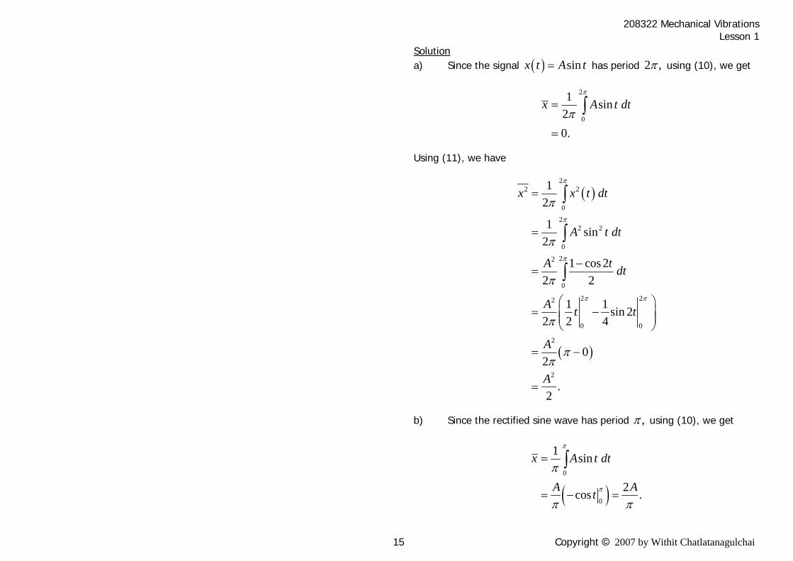
Solutiona) Since the signal ( ) sinx t A t= has period 2 ,π using (10), we get

2

0

1 sin20.

x A t dtπ

π=

=

∫

Using (11), we have

( )

( )

22 2

0

22 2

0

22

0

2 22

0 0

2

2

12

1 sin2

1 cos 22 2

1 1 sin 22 2 4

02

.2

x x t dt

A t dt

A t dt

A t t

A

A

π

π

π

π π

π

π

π

π

ππ

=

=

−=

⎛ ⎞= −⎜ ⎟⎜ ⎟

⎝ ⎠

= −

=

∫

∫

∫

b) Since the rectified sine wave has period ,π using (10), we get

( )0

0

1 sin

2cos .

x A t dt

A At

π

π

π

π π

=

= − =

∫



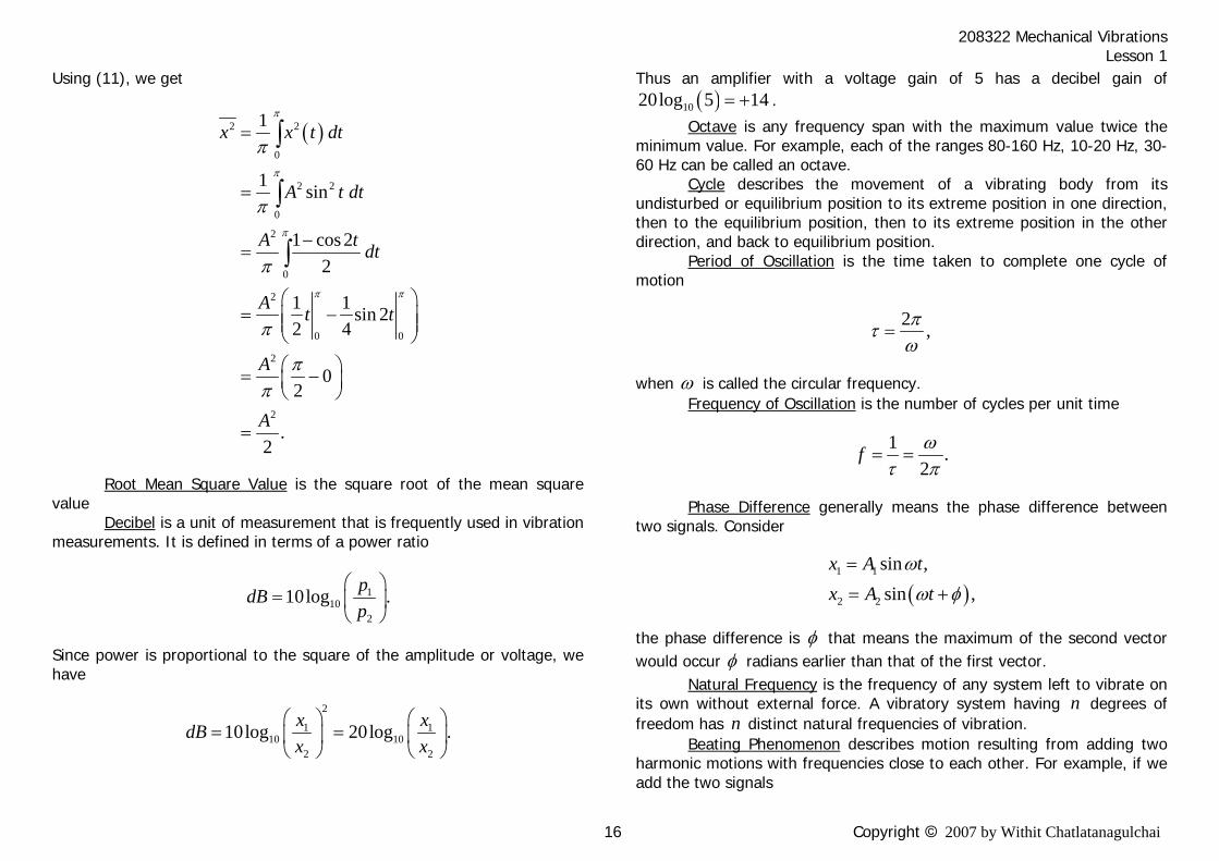
Using (11), we get

( )2 2

0

2 2

0

2

0

2

0 0

2

2

1

1 sin

1 cos 22

1 1 sin 22 4

02

.2

x x t dt

A t dt

A t dt

A t t

A

A

π

π

π

π π

π

π

π

π

ππ

=

=

−=

⎛ ⎞= −⎜ ⎟⎜ ⎟

⎝ ⎠

⎛ ⎞= −⎜ ⎟⎝ ⎠

=

∫

∫

∫

Root Mean Square Value is the square root of the mean square value Decibel is a unit of measurement that is frequently used in vibration measurements. It is defined in terms of a power ratio

110

2

10log .pdBp

⎛ ⎞= ⎜ ⎟

⎝ ⎠

Since power is proportional to the square of the amplitude or voltage, we have

2

1 110 10

2 2

10log 20log .x xdBx x

⎛ ⎞ ⎛ ⎞= =⎜ ⎟ ⎜ ⎟

⎝ ⎠ ⎝ ⎠

Thus an amplifier with a voltage gain of 5 has a decibel gain of ( )1020log 5 14= + .

Octave is any frequency span with the maximum value twice the minimum value. For example, each of the ranges 80-160 Hz, 10-20 Hz, 30-60 Hz can be called an octave. Cycle describes the movement of a vibrating body from its undisturbed or equilibrium position to its extreme position in one direction, then to the equilibrium position, then to its extreme position in the other direction, and back to equilibrium position. Period of Oscillation is the time taken to complete one cycle of motion

2 ,πτω

=

when ω is called the circular frequency. Frequency of Oscillation is the number of cycles per unit time

1 .2

f ωτ π

= =

Phase Difference generally means the phase difference between two signals. Consider

( )1 1

2 2

sin ,sin ,

x A tx A t

ωω φ

=

= +

the phase difference is φ that means the maximum of the second vector would occur φ radians earlier than that of the first vector. Natural Frequency is the frequency of any system left to vibrate on its own without external force. A vibratory system having n degrees of freedom has n distinct natural frequencies of vibration. Beating Phenomenon describes motion resulting from adding two harmonic motions with frequencies close to each other. For example, if we add the two signals



( )( ) ( )

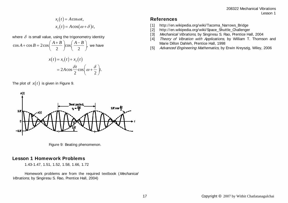
1

2

cos ,

cos ,

x t A t

x t A t

ω

ω δ

=

= +

where δ is small value, using the trigonometry identity

cos cos 2cos cos ,2 2

A B A BA B + −⎛ ⎞ ⎛ ⎞+ = ⎜ ⎟ ⎜ ⎟⎠

we have ⎝ ⎠ ⎝

( ) ( ) ( )1 2

2 cos cos .2 2

x t x t x t

tA tδ δω

= +

⎛ ⎞= +⎜ ⎟⎝ ⎠

The plot of ( )x t is given in Figure 9.

Figure 9: Beating phenomenon.

Lesson 1 Homework Problems 1.43-1.47, 1.51, 1.52, 1.58, 1.66, 1.72 Homework problems are from the required textbook (Mechanical Vibrations, by Singiresu S. Rao, Prentice Hall, 2004)

References [1] http://en.wikipedia.org/wiki/Tacoma_Narrows_Bridge [2] http://en.wikipedia.org/wiki/Space_Shuttle_Challenger [3] Mechanical Vibrations, by Singiresu S. Rao, Prentice Hall, 2004 [4] Theory of Vibration with Applications, by William T. Thomson and

Marie Dillon Dahleh, Prentice Hall, 1998 [5] Advanced Engineering Mathematics, by Erwin Kreyszig, Wiley, 2006


lesson 1 grade breakdown: general information …pirun.ku.ac.th/~fengwtc/teaching/208322 mechanical...

Documents