1.1 Overview of the Lesson The purpose of this lesson is to provide you with a brief overview of Pro/MECHANICA Motion, also called Motion in this book. Motion is a virtual prototyping tool for mechanism analysis and design. Instead of building and testing physical prototypes of the engineering products, you can use Motion to test and refine a mechanism design before you finalize the design and move into functional prototyping stage. Motion will help you design better engineering products in a relatively shorter time. In addition, Motion will provide you with information about the mechanism behavior, which you will usually obtain from tests of functional prototypes. You will be able to modify your design and usually achieve better design alternatives using the more convenient and less expensive virtual prototypes. With such information, you will gain insight on how the mechanism works and why they behave in certain ways. In the long run, this will help you become a more experienced and competent design engineer. In this lesson, we will start with a brief introduction to Motion and various types of physical problems that Motion can solve. We will then discuss capabilities supported by Motion for constructing motion model, conducting motion analyses, and viewing motion analysis results. We will also discuss design capabilities available in Motion, and how to use these capabilities to obtain better designs. In the final section, we will present design examples employed in this book and things you will learn from these examples. Note that materials presented in this lesson will be kept brief. More details on various aspects of mechanism design and analysis using Motion will be given in later lessons. 1.2 What is Pro/MECHANICA Motion? Pro/MECHANICA Motion is a computer software tool that supports design and analysis of mechanisms. Motion is a module of Pro/ENGINEER product family developed by Parametric Technology Corporation. Motion supports you in creating virtual mechanisms that answer the following general questions in product design. An internal combustion engine shown in Figures 1-1 and 1-2 will be used to illustrate these questions. 1. Will the components of the mechanism collide in operation? For example, will the connecting rod

collide with the inner surface of the piston or the engine case during operation? 2. Will the components in the mechanism you design move according to your intent? For example, will

the piston stay entirely in the piston sleeve? Will the system lock up when the firing force aligns vertically with the connection rod and crank?

3. How fast will your mechanism move?

Lesson 1: Introduction to Pro/MECHANICA Motion

1-2 Pro/MECHANICA Motion: Mechanism Design and Analysis 4. How much torque or force does it take to move the mechanism? For example, what will be the

minimum firing load to drive the engine? Note that in this case, proper friction forces and inertia must be added to simulate the resistance of the mechanism before a realistic firing force can be calculated.

5. What are the reaction loads generated on a connection (or joint) between components during

motion? For example, what is the reaction force at the connection between the connecting rod and piston pin? This reaction load is critical since the structural integrity of the connecting rod must be maintained, i.e., the connecting rod must be strong and durable enough to sustain the reaction load in operation.

The modeling and analysis capabilities in Motion will help you answer these common questions realistically, as long as your motion model is properly defined. Motion also supports you in modifying your mechanism to find better design alternatives. The changes that you can make in Motion include component size, geometric shape, mass properties, load magnitudes, etc. Some of these changes will be discussed in later lessons. The design capabilities available in Motion lead you to better design alternatives in a systematic way. A better design alternative can be, for the engine example, 1. A smaller reaction force applied to

the connecting rod; 2. No collisions between components. 1.3 Mechanism and Motion Analysis A mechanism is a mechanical device that transfers motion and/or force from a source to an output. It is an abstraction (simplified model) of a mechanical system. A linkage consists of links (or bodies), which are connected by connections, such as a pin joint, to form open or closed chains (or loops, see Figure 1-3). Such kinematic chains, with at least one link fixed, become mechanisms. In this book, all links are assumed rigid. In general, a mechanism can be represented by its corresponding schematic drawing for

Figure 1-1 An Internal Combustion Engine (Unexplode View)

Figure 1-2 Internal Combustion Engine (Explode View)

Crank Shaft

Piston

Connecting Rod

Engine Case

Piston Sleeve

Piston Pin

Introduction to Pro/MECHANICA Motion 1-3

analysis and design purposes. For example, a slider-crank mechanism represents the motion model of the engine, as shown in Figure 1-4, which is a closed loop mechanism. In general, there are two types of motion problems that you will solve in order to answer those questions. They are kinematics and dynamics. Kinematics is the study of motion without regard for the forces that cause the motion. A kinematic mechanism must be driven by a driver so that the position, velocity, and acceleration of each link of the mechanism can be analyzed at any given time. Usually, a kinematic analysis must be conducted before dynamic behavior of the mechanism can be simulated properly. Dynamics is the study of motion in response to externally applied loads. The dynamic behavior of a mechanism must follow Newton’s laws of motion. The simplest dynamic problem is particle dynamics that you learned in your Sophomore Dynamics, for example, a spring-mass-damper system shown in Figure 1-5. In this case, motion of the mass is governed by the following equation derived from Newton’s second law,

F p t kx c x m x∑ = − − =• ••

( ) (1.1) where (•) appearing on top of the physical quantity represents time derivative of the quantity. For a rigid body, mass properties (such as moment of inertia) are taken into account for dynamic analysis. For example, motion of a pendulum shown in Figure 1-6 is governed by the following equation of motion,

M mg∑ = −•• ••

l l sin = I = mθ θ θ2 (1.2)

Crank

Connecting Rod

Slider (Piston)

Ground

Figure 1-4 Schematic View of the Engine Motion Model

Figure 1-3 General Mechanisms

Ground

Links (Bodies) Connections

(a) Open Loop Mechanism (b) Closed Loop Mechanism

Figure 1-5 The Spring- Mass-Damper System

c k

m

x p(t)

Figure 1-6 A Simple Pendulum

l

θ

x

y

gc.g.

1-4 Pro/MECHANICA Motion: Mechanism Design and Analysis where M is the external moment or torque, I is the polar moment of inertia of the pendulum, m is the

pendulum mass, g is the gravitational acceleration, and θ••

is the angular acceleration of the pendulum. Dynamics of a rigid body system, as illustrated in Figure 1-3, is a lot more complicated than the single body problems. Usually, a system of differential and algebraic equations governs the motion and dynamic behavior of the system. Newton’s law must be obeyed by every single body in the system all the time. The motion of the system will be determined by the loads acting on the bodies or joint axes (e.g., a torque driving the system). Reaction loads at joint connections hold the bodies together. 1.4 Pro/MECHANICA Motion Capabilities Overall Process The overall process of using Motion for analyzing a mechanism consists of three main steps: model creation, analysis, and result visualization, as illustrated in Figure 1-7. Key entities that constitute a motion model include ground body that is always fixed, bodies that are movable, connections that connect bodies, drivers that drive the mechanism for kinematic analysis, loads, and initial conditions of the mechanism. More details about these entities will be discussed later in this lesson. The analysis capabilities in Motion include assembly, velocity, static, motion, and kinetostatics. For example, the assembly analysis brings bodies closer within a prescribed tolerance at each connection to create an initial assembled configuration of the mechanism. More details about the analysis capabilities in Motion will be discussed later in this lesson. The analysis results can be visualized in various forms. You may animate motion of the mechanism, or generate graphs for more specific information, such as reaction force of a joint in time domain. You may query results at a specific location for a given time. In addition, you may ask for a report on results that you specified, for example, acceleration of a moving body in time domain. Two Operation Modes There are two operation modes that you may choose in Motion: Integrated and Independent. The Integrated mode allows you to work in a unified Pro/ENGINEER user interface environment. You can access Motion through menus inside Pro/ENGINEER. You will use the same assembly in both Pro/ENGINEER and Motion. In this case, Motion is considered a module of Pro/ENGINEER, as illustrated in Figure 1-8.

Motion Model Generation

Motion Analysis

Results Visualization

Ground Body Bodies Connections Drivers Loads Initial ConditionsAssembly Velocity Static Motion (Kinematics and Dynamics) Kinetostatics

Animation Graph Query Report

Figure 1-7 General Process of Motion Analysis

Figure 1-8 The Integrated Mode

Pro/ENGINEER

Pro/MECHANICA Motion

Introduction to Pro/MECHANICA Motion 1-5

In the Independent mode, you have two options. You may create an assembly in Pro/ENGINEER and transfer it to the separate Motion user interface (option 1), or you may create your model from scratch in Motion (option 2), as illustrated in Figure 1-9. In option 2, you will have to use less general capabilities to create body geometry. Body geometry is essential for mass property computations in motion analysis. The advantage of using Pro/ENGINEER in either mode of Motion is that the geometry of the bodies can be created conveniently and accurately. When the mass properties of bodies are pre-calculated or pre-measured, creating motion models directly in Motion (Option 2) is more straightforward. Note that the interference checking is only available in the Integrated mode. More details of the differences between these two modes will be discussed in Lesson 3. User Interfaces User interfaces of the Integrated and Independent modes are similar but not identical. User interface of the Integrated mode is identical to that of Pro/ENGINEER, as shown in Figure 1-10. Pro/ENGINEER users should find it is straightforward to maneuver in Motion. As shown in Figure 1-10, user interface window of Pro/ENGINEER, i.e., Motion Integrated mode, consists of pull-down menus, short-cut buttons, prompt/message window, scroll-down menu, graphics area, datum feature buttons, model tree window, and command description area.

Figure 1-9 The Independent Mode

Pro/ENGINEER

Pro/MECHANICA Motion

Figure 1-10 Pro/MECHANICA Motion Integrated Mode

Pull-Down Menus

Short-Cut Buttons

Create New Model

Quit

Graphics Area

Prompt/Message Window

Command Description

Title Bar

Scroll-Down Menu

Datum Feature Buttons

Model Tree Window

1-6 Pro/MECHANICA Motion: Mechanism Design and Analysis The graphics area displays your Motion model. This is where most of the action will take place. The pull-down menus and the short-cut buttons at the top of the screen allow you to manipulate the Motion model. The scroll-down menu supports you in creating and editing your model. As you move the mouse across the menu options, a brief description will appear on the command description area (lower left corner). When you click the menu options, the prompt/message window shows brief messages describing the menu commands and shows system messages following command execution. The Independent mode of the Motion consists of three separate windows. They are Tools Menu and Command Area Window, Work Area Window, and Design Menu Window as shown in Figure 1-11. Each of the windows contains one or more components. Tools Menu and Command Area Window—Located at the top of the Motion screen. This window contains the following components: command area—displays prompts and messages; tool menu bar (pull-down menu)—displays the top-level tool menus; tool button area—displays four tool buttons. This window's title bar displays the version number of the current Motion software release. Work Area Window—This is the graphics window below the command area. The work area displays the current model.

Work Area Window

Design Menu WindowCommand Area

Tool Menu Bar (Pull-Down Menu) Tool Button Area

Title Bar

Tools Menu and Command Area Window

Figure 1-11 Pro/MECHANICA Motion Independent Mode

Introduction to Pro/MECHANICA Motion 1-7

Design Menu Window—Located at the right of the Motion screen. This window displays the current design menu and its ancestors. The Design Menu options allow you to create geometry, build models for your mechanisms, perform analysis and design studies, and review results. The tool menus (pull-down menus) allow you to access various tools, including file utilities, editing functions, and options for displaying entities and creating multiple windows for the work area. The tool buttons are used to access frequently used utilities. These buttons are always visible in the Tools Menu and Command Area Window. Figure 1-12 shows a typical user interface window of both Integrated and Independent modes. The common buttons and options in the window are identified in the figure. We will refer to these buttons and options in the rest of the book. Defining Motion Entities The basic entities of a motion model consist of ground points, bodies, connections, initial conditions, drivers, and loads. Each of the basic entities will be briefly introduced. More details can be found in later lessons. Ground Points A ground point represents a fixed location in space. Once defined, a ground point symbol will appear in the model. You must have at least one ground point in your model. All ground points are grouped as a single ground body. Note that in the Integrated mode, assembly datum points will be converted into ground points automatically. In the Independent mode, you may create your own ground points.

Figure 1-12 Buttons and Selections in a Typical Motion Window

Radio button

Pull-down options

Graphics Area

Text box

Push button

Check box

Display-only text Scrolling list

1-8 Pro/MECHANICA Motion: Mechanism Design and Analysis Bodies A body represents a single rigid component (or link) that moves relative to the other body (or bodies in some cases). A body may consist of several Pro/ENGINEER parts “welded” together. A body must contain a local coordinate system (LCS), body points, and mass properties. Note that body points are created for defining connections, force applications, etc. In Independent mode, geometric points can be created and attached to bodies. In Integrated mode, datum points created for part solid models are converted to body points by Motion. A spatial body consists of 3 translational and 3 rotational degrees of freedom (dof's). That is, a rigid body can translate and rotate along the X-, Y-, and Z-axes of a coordinate system. Rotation of a rigid body is measured by referring the orientation of its LCS to the global coordinate system, which is fixed to the ground body. In the Integrated mode, the LCS is assigned by Motion automatically, and the mass properties are calculated using part geometry and material properties. Body points are essential in creating motion model since they are employed for defining connections and where the external loads are applied. In the Independent mode, you will choose the LCS, and generate the mass properties. The mass properties can be either entered to Motion directly, or calculated from mass primitives you choose for the body. Note that the mass properties of a body are calculated relative to the body’s LCS. The mass primitives available in Motion are sphere, cylinder, brick, cone, and plate. An example of a typical body created in the Independent mode of Motion is shown in Figure 1-13. Connections A connection in Motion can be a joint, cam, gear, or slot that connects two bodies. The connection will constrain the relative motion between bodies. Each independent movement permitted by a connection is called degree of freedom (dof). The degrees of freedom that a connection allows can be translation and rotation along three perpendicular axes, as shown in Figure 1-14. The connections produce equal and opposite reactions (forces and/or torques) on the bodies connected.

Figure 1-13 A Body in Independent Mode

Mass primitives

Center of mass

Body points (Defining joints or forces)

Part schematic

LCS Body1 Body2

Reactions

Joint Rotational dof

Translational dof

Figure 1-14 A Joint Defined in Motion

Introduction to Pro/MECHANICA Motion 1-9

The symbol of a given joint tells the translational and/or rotational dof that the joint allows for the bodies to move relative to each other. Understanding the basic four symbols shown in Figure 1-15 will enable you to read any joint in Motion. More details about joint types available in Motion will be discussed in Lesson 4. Degrees of Freedom An unconstrained body in space has 6 degrees of freedom, i.e., 3 translational and 3 rotational. This is what Motion assumes spatial bodies with 6 dof's per body. When connections are added to connect bodies, constraints are imposed to restrict the relative motion between bodies. For example, a slider joint will impose 5 constraints so that only one translational motion is allowed between bodies. If one of the bodies is a ground body, the other body (slider) will slide back and forth along the given direction (joint axis), specified by the slider joint. The arrow in Figure 1-15a signifies the translational dof that the connection allows. Therefore, there is only one degree of freedom left in this two-body mechanism. In most motion models, you can determine their degrees of freedom using the following formula: D = 6M – N (1.3) where D is the degrees of freedom of the mechanism, M is number of bodies not including the ground body, and N is the number of constraints imposed by all connections. For example, the engine shown in Figure 1-16 consists of four bodies, two pin joints, 1 slider joint, and 1 bearing joint. Pin, slider, and bearing joints impose 5, 5, and 2 constraints, respectively, to the mechanism. According to Eq. 1.3, the degrees of freedom of the engine is D = 6×(4−1) − 2×5 − 1×5 − 1×2 = 1 In this example, if the bearing joint is replaced by a pin joint, the degrees of freedom becomes

(a) Translation⎯Each Arrow Signifies a Translational dof (Slider Joint)

(b) Rotation⎯Single Rotation (Pin Joint)

Figure 1-15 Basic Joint Symbols

(c) Translation and Rotation (Bearing Joint)

(d) No Axes⎯Any Rotation (Spherical Joint)

Ground Body

Shaft Body (Crank)

Piston Body (Slider)

Connecting Rod Body

Pin Joint (Piston/Rod)

Slider Joint (Piston/Ground)

Pin Joint (Crank/Rod)

LCS of Crank

Driver (Crank) Bearing Joint (Crank/Ground)

Figure 1-16 A Complete Motion Model In Exploded View

1-10 Pro/MECHANICA Motion: Mechanism Design and Analysis D = 6×(4−1) − 3×5 − 1×5 = −2 Mechanisms should not have negative degrees of freedom. When using a pin joint instead of a bearing, you have defined joints that impose redundant constraints. You always want to eliminate the redundant constraints in your motion model. The challenge is to find the joints that will impose non-redundant constraints and still allow the intended motion. Examples included in this book should give you some ideas on choosing proper joints. Loads Loads are used to drive a mechanism. Physically, loads are produced by motors, springs, dampers, gravity, tires, etc. A load entity in Motion is represented by the symbol shown in Figure 1-17. Note that a load can be applied to a body, a point in a body, a joint axis, or between two points in different bodies. Symbols of loads applied to joint axis and between two points are shown in Figure 1-18. Drivers Drivers are used to drive a joint axis with a particular motion, either translational or rotational. Drivers are specified as functions of time. The driver symbol is shown in Figure 1-19. Note that a driver must be defined along a movable axis of the joint you select. Otherwise, no motion will occur. When properly defined, drivers will account for the remaining dof's of the mechanism calculated using Eq. 1.3. An example of a complete motion model is shown in Figure 1-16. In this engine example, 26 Pro/ENGINEER parts are grouped into four bodies. In addition, 4 joints plus a driver are defined for kinematic analysis. Types of Mechanism Analyses There are five analysis types supported in Motion: assembly analysis, velocity analysis, static analysis, kinetostatics (inverse dynamics), and motion (kinematics and forward dynamics). The assembly analysis that puts the mechanism together, as illustrated in Figure 1-20, is performed before any other type of analysis. The assembly analysis determines an initial configuration of the mechanism based on the body geometry, joints, and initial conditions of bodies. The points chosen for defining joints will be brought to within a small tolerance. Velocity analysis is similar to assembly analysis but matches part velocities, instead of positions. Velocity analysis ensures that all prescribed velocities of points, including initial conditions are satisfied. Velocity analysis is also computed to within a tolerance. An example of the velocity analysis is shown in Figure 1-21.

Figure 1-17 The Load Symbol

Figure 1-18 Symbols of Special Load

Applied to joint axis

Point-to-Point Load

Figure 1-19 Symbols of Driver

Joint Axes

Driver

Introduction to Pro/MECHANICA Motion 1-11

Static analysis is used to find the rest position (equilibrium condition) of a mechanism, in which none of the bodies are moving. Static analysis is related to mechanical advantage, for example, how much load can be resisted by a driving motor. A simple example of the static analysis is shown in Figure 1-22. Kinetostatics is used to find desired driving loads that produce the prescribed motion of a mechanism. A typical kinetostatic analysis is illustrated in Figure 1-23. Forward dynamic analysis is used to study the motion in response to loads, as illustrated in Figure 1-24. This is the most complicated and common, but time-consuming analysis. Viewing Results In Motion, results of the motion analysis can be realized using animations, graphs, reports, and queries. Animations show the configuration of the mechanism in consecutive time frames. Animations will give

Figure 1-20 Assembly Analysis

Figure 1-21 Velocity Analysis

ω = 200 rpm

ω = ? rpm

V = ?

Figure 1-22 Static Analysis

k1

m g

K2

Figure 1-23 Kinetostatic Analysis

ω

Output: Driving Load p(t)

Input: Prescribed Motion ω(t)

p(t)

Figure 1-24 Forward Dynamic Analysis

ω

Input: Driving Load p(t)

Output: Resulting Motion ω(t)

p(t)

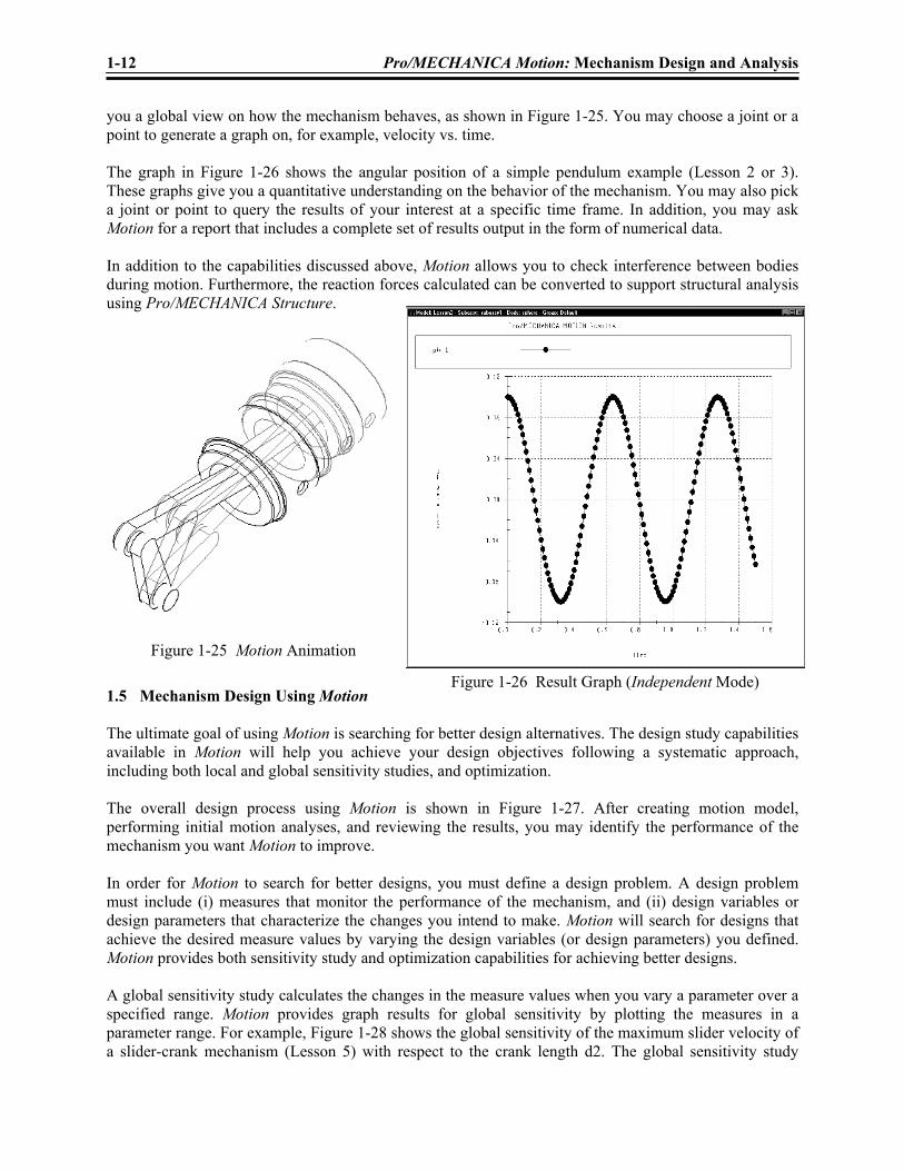
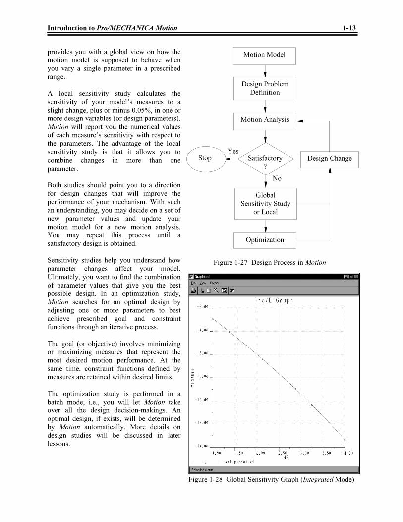
1-12 Pro/MECHANICA Motion: Mechanism Design and Analysis you a global view on how the mechanism behaves, as shown in Figure 1-25. You may choose a joint or a point to generate a graph on, for example, velocity vs. time. The graph in Figure 1-26 shows the angular position of a simple pendulum example (Lesson 2 or 3). These graphs give you a quantitative understanding on the behavior of the mechanism. You may also pick a joint or point to query the results of your interest at a specific time frame. In addition, you may ask Motion for a report that includes a complete set of results output in the form of numerical data. In addition to the capabilities discussed above, Motion allows you to check interference between bodies during motion. Furthermore, the reaction forces calculated can be converted to support structural analysis using Pro/MECHANICA Structure. 1.5 Mechanism Design Using Motion The ultimate goal of using Motion is searching for better design alternatives. The design study capabilities available in Motion will help you achieve your design objectives following a systematic approach, including both local and global sensitivity studies, and optimization. The overall design process using Motion is shown in Figure 1-27. After creating motion model, performing initial motion analyses, and reviewing the results, you may identify the performance of the mechanism you want Motion to improve. In order for Motion to search for better designs, you must define a design problem. A design problem must include (i) measures that monitor the performance of the mechanism, and (ii) design variables or design parameters that characterize the changes you intend to make. Motion will search for designs that achieve the desired measure values by varying the design variables (or design parameters) you defined. Motion provides both sensitivity study and optimization capabilities for achieving better designs. A global sensitivity study calculates the changes in the measure values when you vary a parameter over a specified range. Motion provides graph results for global sensitivity by plotting the measures in a parameter range. For example, Figure 1-28 shows the global sensitivity of the maximum slider velocity of a slider-crank mechanism (Lesson 5) with respect to the crank length d2. The global sensitivity study

Figure 1-26 Result Graph (Independent Mode)

Figure 1-25 Motion Animation

Introduction to Pro/MECHANICA Motion 1-13

provides you with a global view on how the motion model is supposed to behave when you vary a single parameter in a prescribed range. A local sensitivity study calculates the sensitivity of your model’s measures to a slight change, plus or minus 0.05%, in one or more design variables (or design parameters). Motion will report you the numerical values of each measure’s sensitivity with respect to the parameters. The advantage of the local sensitivity study is that it allows you to combine changes in more than one parameter. Both studies should point you to a direction for design changes that will improve the performance of your mechanism. With such an understanding, you may decide on a set of new parameter values and update your motion model for a new motion analysis. You may repeat this process until a satisfactory design is obtained. Sensitivity studies help you understand how parameter changes affect your model. Ultimately, you want to find the combination of parameter values that give you the best possible design. In an optimization study, Motion searches for an optimal design by adjusting one or more parameters to best achieve prescribed goal and constraint functions through an iterative process. The goal (or objective) involves minimizing or maximizing measures that represent the most desired motion performance. At the same time, constraint functions defined by measures are retained within desired limits. The optimization study is performed in a batch mode, i.e., you will let Motion take over all the design decision-makings. An optimal design, if exists, will be determined by Motion automatically. More details on design studies will be discussed in later lessons.

Figure 1-27 Design Process in Motion

Motion Model

Design Problem Definition

Motion Analysis

Global Sensitivity Study

or Local

Satisfactory ?

Design Change

Optimization

Stop Yes

No

Figure 1-28 Global Sensitivity Graph (Integrated Mode)

1-14 Pro/MECHANICA Motion: Mechanism Design and Analysis 1.6 Motion Examples Various motion examples will be introduced in the following lessons to illustrate step-by-step details of modeling, analysis, and design capabilities in Motion. You will learn from these examples both Independent and Integrated modes, as well as analysis and design capabilities in Motion. We will start with a simple pendulum example in the Integrated mode. This example will give you a quick start and a brief overview on Motion. Lessons 2 through 8 focus on analysis and design of regular mechanisms. Lessons 2, 4, 5 use Integrated mode; and lessons 3, 6, 7, and 8 discuss Independent mode of Motion. Design studies will be introduced in Lessons 5 and 7 for sensitivity and optimization studies, respectively. All examples and key subjects to be discussed in each lesson are summarized in the following table. Lesson Title Example Problem Type Things to Learn

2 A Simple Pendulum⎯ Integrated Mode

Particle Dynamics

1. This lesson gives quick run-through of modeling and analysis capabilities in the Integrated mode of Motion.

2. You will learn the general process of using Motion to construct a motion model, run analysis, and visualize the motion analysis results.

3 A Simple Pendulum⎯ Independent Mode

Particle Dynamics

1. The same simple pendulum example is modeled and analyzed in the Independent mode of Motion.

2. You will learn the general process of using Independent mode of Motion.

3. You will also learn the main differences between these two modes.

4 A Slider Crank Mechanism⎯ Initial Assembly and Motion Analyses

Multibody Kinematic Analysis

1. The lesson uses a more general mechanism to discuss joint types, initial assembly analysis, and kinematic analysis.

2. You will learn more about joints and drivers, perform initial assembly analysis, and use Motion and analytical method for motion analysis.

5 A Slider Crank Mechanism⎯ Design Study

Design of Kinematics of Mechanisms

1. The lesson introduces design study capabilities in Motion, including local and global sensitivity studies.

2. You will learn how to define design parameters and measures, conduct design studies, and visualize the design study results.

6 A Slider Crank Mechanism⎯ Independent Mode and Dynamic Analysis

Multibody Kinematic and Dynamic Analyses

1. The lesson discusses modeling and analysis of the same slider-crank mechanism using Independent mode.

2. You will learn more capabilities in the Independent mode, such as defining mass primitives, defining and editing joint types, defining force for dynamic analysis, etc.

Introduction to Pro/MECHANICA Motion 1-15

Lesson Title Example Problem Type Things to Learn 7 A Slider Crank

Mechanism⎯ Optimization Design Study

Optimization Design Study

1. The lesson discusses how to define and run an optimization design study, plus visualize optimization results.

8 Multiple Pendulum

Multibody Dynamic Analysis

1. The lesson introduces multibody dynamic analysis in the Independent mode.

2. You will learn how to create joints, loads, and measures for constructing the multibody system using subassembly capability.

3. You will also learn how to model impact phenomena using force entities supported in Motion.

1-16 Pro/MECHANICA Motion: Mechanism Design and Analysis NOTES: