liens code de la propriété intellectuelle. articles l 122....
TRANSCRIPT

AVERTISSEMENT
Ce document est le fruit d'un long travail approuvé par le jury de soutenance et mis à disposition de l'ensemble de la communauté universitaire élargie. Il est soumis à la propriété intellectuelle de l'auteur. Ceci implique une obligation de citation et de référencement lors de l’utilisation de ce document. D'autre part, toute contrefaçon, plagiat, reproduction illicite encourt une poursuite pénale. Contact : [email protected]
LIENS Code de la Propriété Intellectuelle. articles L 122. 4 Code de la Propriété Intellectuelle. articles L 335.2- L 335.10 http://www.cfcopies.com/V2/leg/leg_droi.php http://www.culture.gouv.fr/culture/infos-pratiques/droits/protection.htm

d'ord.re
THESE
présentée à
L'UNIVERSITÉ NB ldETZFACULTE DES SCIENCBS #
FR MATHÉiUEUQUES, Ii\FORMATIQUE, iUÉCENIQUE
pour I'obtention du rirre de
DOCTEUR
Spécialité :
SCIENCES DE L' INGÉNIEUR(Ment ion : AUTOVIATIQUE)
Par )
Liming WANG rr '
Sujet de la thèse :
GESTION HIÉRARCHISÉE DE SYSTÈMES DE
PRODUCTION DISCRETS: UNE APPROCHE
] BASÉE SUR LES RÉSEAUX DE PETRI. !,., . . . ' t i':. .
Soutenue le 1995 devant le jury composé de : '.
M. Claude LAURENT RapporteursM. Bernard MUTELM. François VERNADAT
Mlle Marie-Clerrrle PÔPTt\rt I xrtrt E-^.ninateUfS
BIBLIOTHECIJE TfTIIVERSITAIRE DE ÆTZ
IffitrHilffiffi$HHHNIo22 420526 5

i . i i : l . .,,,r".r,1:i{;ii
\b IPçt&
GestionDiscrets:
Hiérarchisée de SystèmesUne Apploche Basée sur
Petri
Liming WANG
de ProductionLes Réseaux de
lAs'la

;:!.r.1,r:;ïd:;..'Ë;:.:iÈ:
| : 1 , . : . . r . : : - -
Table des matières
Avant-proposArrière-plan de la thèseContribution de la thèsePlan de la thèseRemerciements
Introduction généralei.1 Gestion de la procluction
l. l . t Systèmes à ér'énernents discretsi.1.2 Systèmes cle production cl isclets1.1.3 Gestion des s1,51,!pes de production discrets
I.2 Introduction aux réseaux de Petri1.2.1 Notions de baseL.2.2 lVléthodes d'analyse générales1.2.3 Réseaux de Petri temporisés
1.3 L'approche proposée
Une hiérarchie à deux niveaux2.1 Approche hiérarchique et approche globale
2.1.1 Approche globale2.I.2 Approche hiérarchique
2.2 ïJn exemple illustratif . . .2.3 lVlodélisation des systèmes généraux
2.3.I Définitions et notations .2.3.2 Positionnement du problème général
2.4 ivlodélisation du système illustratif2 .4.1 L 'exemplere-v is i té2.4.2 Formulation du problème donné en exemple
2.5 Le modèle clu niveau haut2.6 Passage du niveau haut au niveau bas .
2.6.L Désagrégation des familles de produits2.6.2 Désagrégation temporelle et spatiale
2.7 Résultatsnumériques
vl l l
vl l t
ixixÀ
1t
2,J
79
l015r8l 9
2L2I2T22232424252626272830303233

2.7.L Valeurs des paramètres
2.7.2 Résultats et conclusions2.8 Conclusions
Réseaux à sort ies contrôlables et leur simplif ication
3.1 Introduction 38
3.2 Les réseaux de Petri à sorties contrôlables . 38
3.2.L Définit ions 38
3.2.2 Intégration des modules 4I
3.3 Simplification des réseaux de Petri 42
3.3.1 Les T-invariants réduits et leurs propriétés 42
3.3.2 La simplification des modules 43
3.3.3 Détermination de la famille génératrice des T-invariants réduits 44
Modélisation modulaire et gestion hiérarchisée 46
4.i rVlodélisation à I'aide des RdP 47
4.2 Modélisation modulaire . 49
4.3 Gestion hiérarchisée . 52
4.4 Présentation du loeiciel H\'IPS t:J
Evaluation de I 'approche5.1 Exemplesi l lustrati fs5.2 Application industrielle .5.3 Conclusions
Conclusions générales et6.1 Conclusions générales
perspect lves
6.2 Perspectives
Control lable-Output Petri netsA.1 Basic notions and properties of CO nets
4.1.1 Definition of CO netsA.1.2 Propert ies of CO nets
A.2 System integrationA.3 Identification of CO net
A.3.i Some condit ions for H5A.3.2 Identification algorithm .
A.4 Concluding remarks
Simplif ication/Reduction of module models8.1 Computation of minimal support T-invariant . . .
8.2 Reduced T-invariant: definition and properties8.2.1 Definition of reduced T-invariant .
8.2.2 Properties of reduced T-invariant . .
.:1,i;.:-;.;-1;-:.i:; i", ' ''1 - . ' l . - . . . ; .
333337
38
O D
ôD
5963
6464
686868707277t t
R'
84
8585868787

B.3 Computation of reduced T-invariant '8.3.1 Two schemes of aggregation8.3.2 A preliminary result8.3.3 Acyclic Petri nets rvith input and output transitions
8.3.4 General Petri nets8.3.5 Efficiency of the algorithms
8.4 Concluding remarks
Modular modell ing and hierarchical management
C.1 System representationC.2 System modelling by means of Petri nets 108
C.3 Modular modell ing 111
C.+ S)'stem features 114
C.5 Hierarchical management scheme 115
C.6 Capacity evaluation 118
C.6.1 Relevant notations 118
C.6.2 Evaluating s.v-stem capacit5' 1i9
C.6.3 An approximation of system capacity 120
C.7 Simplified rvhole s-rrstetl planning 121
C.8 Cell planning ancl cell scheduling 123
C.9 Computational experieuce I21
C.9.1 Capacity evaluation L2+
C.9.2 Solving a concreie example 126
Package HMPS (Hierarchical anrl tr[otlular approach to production Plan-
ning and Scheduling) 130D.1 Introduction to language Tcl/Tk 130
D.2 The package HMPS 131D.2.1 HMPS versus N4ASP I32D.2.2 Atctriteclule of HN'IPS . . I32D.2.3 Defining a model 133D.2.4 Building an executive product base 136D.2.5 Defining cells 136D.2.6 Specifying demands and getting results for planning . ' . I37D.2.7 Scheduling the cells L4I
D.3 Conclusion L43
9090919398
102103
104105
Bibliographie
Index
L45
156
l t I

Table des figures
1.1 Système de production et son environnementI.2 Système de gestion, système de production et environnement1.3 Une structure décisionnelle à trois niveaux
Un exempleLe système obtenu enNotations définitives
supprimant les premiers stocks
Niveau haut2.5 Essai I2.6 Essai I I2.7 Essai I I I2.8 Essai IV2.9 Essai V
3.i Trois réseaux de Petri
Schématisation du processus "horizon glissant"Deux gammes de fablicationLe RdP corresponclant aux deux gammes de fabricationLe modèle cl'ordonnancementiVlodèle RdP de la cellule C1 et sa simplificationModèle RdP de la cellule Cz eL sa simplificationModèle RdP de la cellule Cs et sa simplificationIntégration des modèles simplifiés
Valeurs critères des tests SE, SS, et SANIHTemps de calcul pour tests SE, SS, et SANIHGamme pour Pr à Pzs
2.r2.22.32.4
4.r4.24.34.44.54.64 .74 .8
40
17
68q
232326283.r35353636
48495050515152
DÙ
5960
6973737878
5.15.25.3
4.14.24.34.44.5
CO nets and non-CO netsA typical structure of system integrattonA contracted graphA non-oriented pathThe insufficiency of " no non-oriented path" condition
I V

8.1 An illustrative Petri net8.2 An illustration of aggregation schemesB.3 Integration of trvo Pebli nets by transition merging8.4 Decomposition of an acyclic Petri net into layers
8.5 Cross-layer connections .8.6 Elimination of cross-layer connections8.7 Removing cross-layer connections8.8 G(2) and G-(2)8.9 G'(3) and G.(3)8.10 G' , (4)8.11 An elementary transfolmation to obtain ac1'-clic Petri net
8.12 A Petri net rvith seven la.u-ers rvith S: {tr, tz} . .
B.13 Elimination of closs-layer connections from lorv la1'er nodes to high
laver nodesB.14 Nlodel obtainecl by removing cross-la1'er connections 100
B. I5 G' (2) and CJ-(2) rv i th sz = { t r ,Js, ls} 101
8 .16 G ' (3 ) anc l G- (3 ) r v i t h ,S3 = { t r , r5 , l 6 , l r o } 101
B.lT C;'(4) and CJ"(a) rvith ,5'4 = { lr, tz} . . 102
C.l Transtbrmation opelations 105
C.2 Transformation operations in series 106
C.3 An assemblv operation 106
C.4 A disassembl) 'operation 106
C.5 BOTVIs for Pr, Pz, Pt 107
C.6 PN models for tlansformation operations 109
C.7 PN model fbr assembl,v'operations 109
C.8 Petri net models for Pr, Pr, P" 110
C.9 Decomposing cancatenated transformation operations Il2
C.10 Decomposing a transformation operation 113
C.11 Decomposing an assembly operation . 113
C.12 Petri net model for cell I . . . IL4
C.13 Petri net models for cel ls 2 and 3 . . 115
C.14 lvlodular modelling 116
C.15 Hierarchical planning Il7
C.16 Petri net model for the simplified rvhole system LI7
D.1 Title of the package .D.2 The ma.in ûlenuD.3 Defining a modelD.4 Input a model as BOlvlD.5 Precedence constraint specificationD.6 Choosing an executive procluct base from a product base fileD.7 How many and rvhich pt'ocesses to choose
87929294949595969797oo
99
t00
L32133134135135136137

D.8 Cell definitionD.9 New look of main mentl after cell definitionD. l0 Objective functionD.11 Planning parametersD.12 Interface informationD.13 Results for simplified system planning and cells planning
D.14 New look of main menu after planningD.15 Scheduling menuD.16 Scheduling result 143
138139140140141147r42142
vl

Liste des tableaux
1.1 Classification cles Nloclèles cles Systèmes à Événements Discrets .
I .2 Nléthodes de réduction
2.I Temps opératoiles .2.2 Essai I: Denancles poul P1, ' ' ' , Po2.3 Essai I I : Demandes poul P1 , ' ' ' ' P,2.4 Essai I I I : Demandes pour P1, ' ' ' , P,2.5 Essai IV: Demancles pour P1 . ' ' ' , P,
5.1 Dettx groupes d'exemple5.2 Plemiel test5.3 Deuxième test5.4 Troisième test5.5 Temps élémentair-es pour- Pt à Pzo5.6 Temps élémentaires poul P21 à P2s5.7 Demandes cles pt'oduits (rnensuelles)5.8 Coûts de stockage et coûts cle rupture
C.l Correspondence betrveen reduced T-inv. and transitions L24
C.2 Definition of p . I24
C.3 Demands informabion 126
C.4 Initial inventory 126
C.5 Inventory costs ancl backlogging costs L27
C.6 Interface information L27
C.7 Simplified whole system planning results L27
C.8 Plan for cell 1 \27
c.g Plan for cell 2 I27
C . l 0P lan fo r ce l l 3 . . . 128
4T7
33:14')+
3536
coô t
57ôô
61616262
C.11 Schedule for cellC.12 Schedule for cell
(by means of SA)(by means of BAB)
128L29
I
I
1
v l l

Avant-propos
Arrière-plan de la Thèse
Dans un appel aux communications d'r:n congrès international (IJCAI'95: In-
telligent l,Ianufacturing System.s) sur les systèmes de production, on peut lire:
Global competition ancl rapid technological advances in communi-
cation, computing. ancl flexible machinery ale bringing about unPre-
cedented changes in manufactuling a.nd management practices. The
global manufa,ctttt'ittg companl' of the futule rvill have Lo be lean,,
customer-driuen. en,uir-on,nten,t-cottsciotL.s. It lvill have to be capable
of rapidly adapting its ploducts, processes and alliances in leaction to
changes in marliet demands, technologies, raw material availabilities,
legislations, etc.. As companies strive to attain these elusive objec-
tives, they are turning to radically nelv manufacturing philosophies
and concepts, e.g., Lean lvlanufacturing, Agile Vlanufacturing, Virtual
iVlanufacturing, Holonic Nlanufacturing, etc.. It is expected that Arti-
ficial Intelligence, Opera.tions Resealch, Control Theory, and Informa-
tion Technolog-v rvill plai' a liev role in delivering the decision support
tools required to turn these visiona,ry' concepts and philosophies into
practice.
Ce résumé des tendances montre bien clue Ia complexité des systèmes de pro-
duction va en croissant. et donc qu'une modélisation minutieuse prend tous lesjours plus d'importance. Cela justifie les travaux que nous présentons ici.
Cette thèse a été préparée au sein du projet SAGBP de I'INRIA-Lorraine sous
la clirection scientifiqtre de Nlonsieur Jean-lvla,rie PROTH, Directeur de Recherche
à I ' INRIA.Le projet SAGEP a pouï objectif l'étude cles problèmes induits par le contrôle
cles systèmes dynamiques, et en particulier des systèmes à événements discrets. Le
domaine d'application privilégié de nos travaux est celui des systèmes de produc-
tion industriels.
v lu

- . ' . : ; i . . i l : r : . ; i
Contribution de la Thèse
La gestion de la production aboutit à I'ordonnancement. L'ordonnancementconsiste à affecter les tâches aux ressources, et à décider les dates auxquelles cestâches vont débuter, en tenant compte des contraintes inhér'entes à la productionmanufacturière. Un tel problème est généralement NP-difficile, ce qui interdit dele résoudre sur un horizon sufÊsant pour prendre en compte les fluctuations dela demande. Un moyen possible pour contourner cette difficulté est d'utiliser uneapproche hiérarchique et de faile évoluer le système en suivant le principe desplans glissants.
Nous verrons, clans le chapitle 2, c1u'une abondante littérature existe sur cesujet. Cependant, une apploche sSrstématique de la conception d'une hiérarchiereste à trouver. Il nous semble clue les réseaux de Petri, et plus particulièrementun type de réseaux de Petri appelé réseaux de Petri à sorties contrôlables (COnets en anglais; CO signifie " Controllable-Output" ) sont particulièrement efficacespour nous accompagner daus cette démarche.
Dans notre travail, nous présentons d'abord un exemple simple de hiérarchieà deux niveaux. Il pelmet cl'iilustr-el les ar.'antages et les inconvénients d'une ap-proche hiérarchique.
Nous passons ensuite à une étucle approfondie des "CO nets", et nous mon-tlons que les réseaux CO constituent un outil satisfaisant pour notre approche,laquelle est à la fois modulaire et hiérarchiclue. Nous développons une méthode desimplification des modules et montrons comment intégrer les modules simplifiéspour conserver les propriétés clualitatives souhaitées.
Enfin, nous établissons une démarche descendante qui consiste à résoudre lemodèle global simplifié sur un horizon suffisamment grand, puis à se servir de lasolution obtenue comme contrainte à satisfaire par les modules détaillés du niveaubas sur un horizon réduit.
Ce travail peut être considéré comme une tentative de rationalisation de lagestion hiérarchisée.
Plan de la Thèse
Cette thèse est organisée comme suit:
- Le chapitre 1 est consacré à une présentation générale des réseaux de Petriet de la gestion de production. Les notions de base, ainsi que les approchesd'analyse et différentes classes de réseaux de Petri, sont présentées. Les basesde la gestion des systèmes de production discrets sont rappelées dans cemême chapitre.
- Dans le chapitre 2, nous comparons I'approche hiérarchique et I'approchemonolithique pour- la gestion de production à I'aide d'un exemple simple
' ; ' : , r , ' - l.:.l1 ..,":
l x

: . , : . : . : , 4 ; :. i ,+ : r_ - : - . + _+-ae, r ' i+ !3 .s -q
, r , . . ; : . t , . r : - . . ; . f - È : :
mais significatif. Cette étude comparative permet de justifier I'utilisation
de I'approche hiérarchique pour la gestion de systèmes complexes. Une ap-
proche hiérarchique à deux niveaux poul la planification de la production
est également présentée pour illustrer le concept.
- Dans le chapitre 3, nous proposons Ia notion de réseaux de Petri à sorties
contrôlables (réseaux CO) et étudions les propriétés des réseaux CO. Nous
étudions aussi la réduction/simplification d'un réseau de Petri. Nous propo-
sons quelques algorithmes pour atteindre cet objectif et, en particulier' nous
proposons un algorithme qui permet de traiter les réseaux de Petri généraux.
- Dans le chapitre 4, nous étudions Ia modélisation modulaire et la gestion
hiér'archique des systèmes cle procluction cliscrets à I'aide des réseau-x de Pe-
tri. Nous présentons a.ussi. dans ce chapibre, I'a,rchitecture du logiciel HTVIPS
(en anglais Hierarch,ical tntl tr'[odular opytroach to production Planning and
Scheduling) développé au sein cie l'écluipe SAGEP cle I'INRIA-Lot'raine.
- Dans le chapitre 5, nous évaluons I'approcire que nous avons proposée. Selon
les résultats des tests affectués. nous constatons que I'approche est efficace
poul les problèmes que nous avons rencontr-és dans la pratique.
- Le chapitre 6 est la. conclusion. Nous 1' présentons en particulier les exten-
sions possibles de notle travail.
Remerciements
Je tiens à remercier tous les membres du jur,v.
Je tiens à exprimer toute ma reconnaissance à ùlonsieur Jean-lVlarie PROTH
pour la confiance qu'il m'a accordée tout a,u long de cette thèse, ainsi que ses
conseils qui m'ont permis de progresser dans mon tlavail.
J'aclresse mes plus vifs remerciements à il'lonsieur Xiao-Lan XIE, Chargé de
Recherches à I'INRIA et habilité à diriger des recherches, pour I'aide qu'il m'a
apportée tout au long de ce travail.J'exprime également ma symPathie à bous les membres I du projet SAGEP,
ainsi qu'à Evelyne Agostini, pour l'aide et la bonne humeur dont ils font preuve
quotidiennement. En palticulier', je remercie C. Bouton, F. Chu, V.M. Savi pour
Ieurs aides dans la réalisation du logiciel HI'{PS. Je remercie aussi P. Fournet-
Fayard pour son aide sur I'usage de I4$X.
1. Julien Antonio, ChristopheFournet-Fayard, Nathalie Sauer,Philippe Wolfl
Bouton, Christel Carmier, Chengbin Chu, Feng Chu, PierreVanio Nlurilo Savi, Abdelghani Souilah, François Vernadat,

Chapitre 1
Introduction générale
La concurrence internationale, un marché où I'économie d'envergure a remplacél'économie d'échelle. et une clemande cle plus en plus forte de qualité, ont conduità concevoir des s,u-stèmes cle production de plus en plus sophistiqués. Les maîtresmots sont clésormais automatisation, intégration des fonctions de I 'entreprise,gestion hié'-archisée cle la procluction, flexibilité, c'esb-à-dire capacité de passer
rapiclement d'une procluction ir une autre, et modularité, laquelle facilite la re-structuration des systèmes de ploduction. Poul faire face à cette situation dans debonnes conditions de compétitivité, I'industrie fait appel à des systèmes à la foisadaptatifs et automatisés: les ateliers flexibles (en anglais: Flexible Manufac-turing Systems, en abrégé: F\,IS). Les systèmes automatisés et flexibles, tels lesateliers flexibles, permettent de fablicluer une grande variété de produits. en petites
et moyennes séries, grâce à I'utilisation de ressources multi-tâches. La conséquencede cette évolution est une complexité cloissa,nte des systèmes de production et deleur systèmes de commande. Cette ér'olution a rendu nécessaire le renforcement dela phase de conceplion préliminaire. encore appelée "étude papier". Cette étudepapier englobe I'ensemble cles activités qui vont de la spécification des produitsque I'on veut fabriquer à la spécification du système qui sera chargé de cette fa-brication. Elle contient, sans pour autant s'y limiter,la spécification fonctionnelle,la modélisation, l'évaluation et la spécification de la commande du futur système.
[105] [1 i4 ]Un problème fondamental rencontré dans les systèmes automatisés et flexibles
est de trouver le bon compromis entre les deux clualités antagonistes que sont unebonne productivité et une grande flexibilité. Une solution partielle du problèmese trouve dans la gestion cle ces systèmes.
Selon r-rne évaluation faite dans I'industrie aérospatiale el automobile,les progrès
de la recherche a,u niveau exécubion (serveur/actuateur) peuvent conduire à l-2Tode réduction du coût global, alors que les progrès de la recherche au niveau organi-sateur (planning, ordonnancement) peuvent conduire de 25 à 33% d'améliorationdu cofit global [55].
La gestion des systèmes de procluction est un vaste domaine qui s'intéresse

:,jr :r;#c- ri!::ri ri: ::::r-
r : . ' + . ,
à I'ensemble des décisions à prendre pour assurer le bon fonctionnement d'un
système cle production. Des outils ont été développés afin d'aider aux prises de
décision, du niveau le plus haut (stratégie génétale de I'entreprise) au niveau Ie
plus bas (fonctionnement cles machines dans I'atelier de fabrication) [3a].Notre travail concerne les systèmes de production discrets. L'outil que nous
utilisons est les réseaux de Petri (RdP) [100][109][68].Puisque I'objectif de cebte thèse est d'étudier la gestion des systèmes de pro-
duction discrets dans un enrrironnement réseaux de Petri, nous présentons d'abord
une introduction aux s,v-stèmes de procluction discrets, dans laquelle nous donnons
une vue globale de ce domaine. Puis nous intloduisons la théorie des réseaux de
Petri en nous limitant aux aspects qui seront utiles dans la suite.
La relation entre les réseaux de Petli et les s,u*stèmes de production automatisés
est clairement expliquée dans des articles [120] et [3].
1.1 Gestion de la production
Une des caractér'isticlues tbndamenta,les des systèmes de production que I'on
rencontre clans I'inclustrie rnanufactttrière est la nature rliscrète du processus de
tâbrication. Les occurrences cles ét'énem672l-s qui ploduisent les changemenbs d'état
clu système clépenclent cle plusieurs fa,cteurs: I'orclre par-tiel entre les différentes
tâches imposé pal les contraintes technologiques, les durées réelles des opérations
(i.e. conbraintes tempor:el les), et la disponil l i l i té des ressources. Un tel systèmeest
un système à événements cliscrets (SED).
On note que les caractérisbiclues des systèmes automatisés et flexibles se ren-
contrent dans d'autres domaines, notamment celui des s5rstèmes informatiques'
Bien que les paramètres ne soienl pas les mêmes, les systèmes informatiques
sont également des systèmes multi-tâches et multi-ressources, et les problèmes
qui se posent dans ce domaine s'expriment en termes de coordination d'acti-
vités parallèles asynchrones. cle conflits de ressources, et de contraintes tempo-
relles strictes. C'est pourquoi les outils d'évaluation employés aujourd'hui pour
les systèmes de production sont au ca,rrefour de plusieurs domaines d'application
[60] [105] .Il faut noter cepenclant que certaines caractéristiques, en particulier I'impor-
tance des débits, font que les outils disponibles n'ont pas la même efficacité en
production manufactutière et en informatique.
1.1.1 Systèmes à événements discrets
La théorie des systèmes traclitionnels est principalement consacrée à l'étude des
systèmes continus, dont les comporternents peuvent être décrits par des équations
aux différences finies, cles écluations différentielles, ou des équations aux dérivéespartielles. iVlalheureusement, il est impossible d'utiliser ces équations pour décrire

. , - . * .- . , . , , . : : . . , . . . . . , - : ,r,-*jr-\Yls#; r; F-l*- =n"
. : , - r , i i - : È : .
. .- -l a-..++lrr . :a- -, " . - -
.:,ii :li-j!!,
le comportement dynamique d'un système à événements discrets et, en particulier,
d'un système de production. La même remarque s'applique aux réseaux de commu-
nication, aux réseaux d'orclinateurs, aux réseaux de transpolt: bien que différents
des systèmes de production, ils ont des comportements qui en font également des
systèmes à événements discrets [27][6t] [73] [106] .Lorsque I'on observe un système à événements ctiscrets, on constate que son
état n'évolue qu'en des points discrets du temps. L'évolution d'un SED est donc
caractérisée par une séquence d'états et par la dulée de chacun d'eux. La combi-
naison de la nature discrète cle I'espace cles états et de la nature continue de leur
durée est une des difficultés de I'analyse des SEDs. D'autres difficultés sont:
- la présence de perturbations et d'interactions entre les sous-systèmes du
système étudié,
- I'explosion de I'espace des états: habituellement le nombre d'états d'un SEDcroît de manière exponentielle avec le nombre de ses composants,
- la variété des champs cl'application cles s-v'stèmes à événements discrets.
Pour ces Laisons, il est clilfcile de lburnir une apploche analy'ticlue unifiée dans
l'étude des sirstèmes à événements discrets.Les modèles des systèmes à événements cliscrets sont cle cleux types: les modèles
temporisés et les moclèles non temporisés. Les modèles non temporisés servent à
étudier les propriétés clualilatives telles clue I'absence de blocage, la vivacité, la
réversibi l i té etc. (Voir, e.g., [37] [105] [106] [10i] [120]). Les modèles temporiséssont utilisés pour l'évaluation des perfoïmances et pour I'optimisation du compor-tement des systèmes.
A ces deux types de moclèles correspondent respectirrement deu-x types de
travaux: les études logiques el les études des performances. Les études logiques
s'adressent à la description causale des comportements des systèmes. Les étudesdes performances s'adressent à l'évaluation des performances des systèmes. Elles
sont basées sur la théorie des probabilités et les techniques stochastiques. Le Ta-
bleau 1.1 donne une classificabion des modèles les plus connus [27] [61]. Dans le
Tableau 1.1, on voit que les réseaux de Petri sont un outil complet qui permet
de supporter la modélisation, I'analyse et l'évaluation des systèmes à événements
discrets [105] [130], car les réseaux de Petri peuvent servir à l'étude logique et à
l'étude des performances d'un système..Ramadge et Wonham [106][107] ont introduit la théorie du langage formel
et les automates pour étudier les systèmes à événements discrets. Ils ont étudié
en particulier le problèrne de supervision de ces systèmes. Ce problème consiste
à déterminer un contrôle aussi peu contraignant que possible pour que le com-portement du système satisfasse des conditions imposées décrites par un langagelégal. Un langage légal spécifie un ensemble de comportements admissibles. Les
concepts du contrôle classique tels que la contrôlabilité, I'observabilité, le contrôle

, : . - : :' . ' . i .r ' ,t
Temporisé Non temporisé
LogiqueAutomates,
Processus récursifs.RdP, etc.
PerforrnanceRdP temporisé,
Algèbre max-plus.Simulation. Fi les d'attenteAntoma,tes tempolisés. etc.
Tns. I.1 - Classi.fication. des X.'[orlèles des Systèmes à Euénements Discrets
décentralisé et le contrôle hiér'archiclue sont étudiés. Une extension aux modèlestemporisés a été étudiée dans Ostroff et Wonham [9i] à I'aide de la théorie de
logiqtre temporelle(real ti me temporul logic).Cohen et al [30][31] ont utilisé I'algèb.-e max-plus[33] pour modéiisel et analyser
les systèmes à événernents cliscrets. Ils ont fait apparaître cles propriétés similaires
entre les modèles d'algèble max-plus et les sy,'stèmes linéaires aux sens du contrôleclassiclue. L'inconvénient principal cle ce moclèle est sa faible puissance descriptive.
Inan et Varaiya [66] ont proposé des modèles FRP (Finitely Recursiae Process
models). Ces modèles sont basés sur la théorie des CSP (Communicating SequentialProcesses [63]). Un système à événements discrets est représenté par un ensembled'équations récurrentes et la trajectoire de l'état du système est générée de manièreitérative par rapport au temps. Les modèles FRP ont une grande puissance, ce qui
permet cle décrire une famille plus importante cle systèmes à événements discretsque les techniques précédentes.
L'utilisation des files d'attente pour les problèmes d'analyse et d'évaluation des
systèmes de production, et plus particulièr'ement les ateliers flexibles, fait I'objetd'une abondante littératule [25] [24]. Les réseaux de files d'attente sont adaptésà l'étude du fonctionnement en régime permanent lorsqu'il s'agit d'obtenir des
résultats en première approximation sur le comportement du système, ou bienpour résoudre certains problèmes qui se posent à un niveau "haut" de la ges-
tion (problèmes de flux). La littérature abondante qui traite des chaînes de IVIar-kov justifie les développements qui concernent les files d'attente. L'extension desprocessus Markoviens conduiI aux pr-ocessus semi-lVlarkoviens, e.g., GSMP (Ge'neralizecl Serni-ùlarlcou Proces.ses)[a7][a6], clans lesquels un temps cle distributiongénérale est associé à chaclue événement. Le concept de dérivée qui joue un rôleprédominant dans la théorie de contrôle classique fait I'objet cle nombreuses études
,r i*l-.

- . : ' . ! . ' : . l l .
appelées communément I'Analyse des Perturbations (Perturbation Analysis)1621.Le souci principal de I'analyse des perturbations est d'estimer les gradients desfonctions dont les valeurs sont obtenues par simulation.
Largement utilisée clans la pratique, la simulation a I'avantage de s'appli-quer à n'importe quel type de système, aussi complexe soit-il. Au niveau dela fi.nesse des résultats obtenus, la simulation reste incontestablement le moyend'évaluation le plus puissant. Les langages de simulation sont nombreux (plusd'une centaine), mais les plus connus restent WITNESS [64], SIMAN [99], SI-MULA [15], GPSS[49], et SLAI{ II [96]. I ls permettent d'exprimer le modèle sousforme d'un programme dont les entrées représentent le contrôle et les demandes.Si ce programme représente ficlèlement le système. son exécution rend possiblela connaissance du compoltement cle ce système sous différentes hypothèses decontrôle. Quand il s'agit d'optimiser les performances du s.u-stème, la simulationoffre donc peu de recoul's. Sans prétendre aborder en détaii les problèmes liés à samise en ceuvre, on reconnaîtra cependa,nt I'inconvénient majeur de la simulationen raison cle son aspect boîte noire: on définit des paramètres et on obtient desrésultats, mais sans aucune infor:rnation sur la façon dont les résultats dépendentdes valeurs des paramètres. Bien entendu, cela n'est plus vlai si I'on superposeI'analyse des perturbations à la simulations.
Grâce à leuls représentations graphiques faciles à comprendre et à utiliser parles ingénieurs, les réseaux cle Petri l [23] [92] [100] [109] tburnissenb un outi l simpleet efficace pour la modélisation des systèmes à événements discrets. Les réseaux dePetri tempolisés permettent de prendre en compte de manière simple les duréesdes activités d'un s,u*stème à événements discrets. Les réseaux de Petri ont éiéutilisés pour la modélisation et I'analyse des systèmes de production automatisés
[54] [59] [56] [74] [104] [103] [102] [105] [120], des protocoles de communication
[113 ] , e t c . .Il est utile de noter que I'exposé que nous venons de présenter n'est pas com-
p[et. L'objectif est de donner un aperçu de la recherche autour des systèmes àévénements disclets et, en particulier, de la gestion des systèmes de productiondiscrets, laquelle est notre principal intérêt de recherche.
L.L.2 Systèmes de production discrets
Un système de production dépend fortement de son environnement, en parti-culier de ses fournisseurs et de ses clients. La Figure 1.1 illustre cette dépendance.
D'un côté, les fournisseurs alimentent le système de production suivant lesdécisions prises par le système de gestion (voir aussi la Figure L.2). La matièrecircule ensuite dans I'atelier de production entre les ressources et les stocks. Enfin,les produits finis sont stockés jusqu'à la livraison aux clients.
) : i i '
I 'Nous présentons en plus de détail le daus la section 1.2.

i,f :;,i;d;;;.,,,:;,,,.:.,:;,.:ç..3;3;1i";.li::i==; : , . . . , ' . , : , r : t : : ' . : - , : l , i ; . r ; , , . t ' r t - r , : ! . : ; , ' : . , .1 r . : : , , ; . i
+r Fluxdcmatâicls
FIc. 1.1 ' Système de production et son enaironnernent
Un système de production contient toutes les ressources nécessaires, tant hu-maines que matérielles, qui permettenb de transformer la matière première ou/et
les composants en produits finis. Les systèmes de production sont organisés etgérés en fonction des dema,ndes et des ressoulces disponibles.
II existe une grande diversité de systèmes de production. De nombreuses typo-logies ont été proposées dans Ia littératr.rre [9i]. N,Iêmesi elles ne sont pas uniqueset peuvent êtle discutées, deux ty-pologies nous semblent intéressantes pour ca-
ractér'iser un système de ploduction [45].La première typologie clistingue les systèmes da,ns lesquels la production est
déclenchée par les comma,ncles des clients (production à la demande, rnake-to-order), et ceux dont la procluction peut s'effectuer en anticipant des demandes(production prévisionnelle, make-to-stock).
La production à la demande concerne principa.lement les entreprises fa-bricant une grande variété de produits dont la demande est trop aléatoire, et lesenbreprises qui ne définissent leurs procluits qu'à partir de clemandes précises desclients. Les sociétés de sous-tlaitance sont des exemples palfaits de cette catégorie
[34].La production prévisionnelle n'est possible que pour des entreprises qui
fabriquent les produits dont la demande reste relativement stable et prévisible.Par exemple, les productions alimentaires sonb à classer dans cette catégorie.
Bien entendu des situations intermédiaires existent: dans certaines firmes au-tomobiles les voitures sont commencées sur la base du " rnake-to-stoclC' et sontcomplétées au vu des commandes des clients.
La production prévisionnelle conduit à des modèles déterministes ou stochas-tiques de gestion de stocks. Parmi ces modèles, on trouve en particulier les fa-meuses quantités économiques, qui assurent un compromis optimal entre les coritsde stockage et les coûts de changement de fabrication [13] [38] [134].
La deuxième typologie est basée sul le type de production. Elle distingue quatre
catégories de systèmes [12] [3a]:
- La production unitaire: dans un s5'stème de ce type, la fabrication dechaque produit est longue et coûteuse. La tâche principale consiste à réunirles moyens nécessaires au bon moment et au bon endroit. Ce type de pro-duction utilise les techniques de l'ordonnancement de 'projets.
t :
ii: j,';.,É.

l u , , r * - " , q i - 1 ! 1 t L r F - . - * l - Î È + . l J + . ' :
.
I ' .: . i : i ..
i . .. j ;:: i ,r i1t:: i.1.. .:,.a-;;...1.:i , : i . . i , . ,z
::t::lI:
- La production en petites et moyennes séries: de volume faible, le pro-
duit se déplace dans un atelier de production. Le problème consiste souventà minimiser, non pas le temps de fabrication d'un seul produit, mais ce-
lui de I'ensemble de la production, cet objectif coîncidant souvent avec la
minimisation des temps d'attente devanb les ressources.
- La production en grande série: dans le cas orl le nombre de produits simi-laires à fabriquer clans les mêmes délais devient très important, ii est rentablede constituer des chaînes de fabrication (les ressources sont placées dans unordle précis et inamovible). Celles-ci peuvent entraîner une meilleure pro-
ductivité. La constitution de chaînes équilibrées est un élément primordialdans la réussite de ce type de production.
- La production en continu: ce t1''pe de ploduction interdit toute possi-
bilité d'attente entre cleux ressources. Il concerne surtout une fabricationnécessitant la manipulation de matières liquides ou gazeuses. Là encore, Iadéfinition de la chaîne est souvent l'élément essentiel du bon fonctionnementde la production.
Dans ce travail, nous nous intéressons aux systèmes de production discretsfonctionnant en préui.sionnel ou à la t lemande eL en petites et moyennes séries.
1.1.3 Gestion des systèmes de production discrets
Le système de gestion à pour rôle d'assurer en permanence la bonne utilisa-tion de I'ensemble des moyens de procluction. Poul bien gérer, les décisions prises
doivent être basées sur des informations actualisées (ressources disponibles. situa-tion des clients et des foulnisseurs). Un bon système de gestion est caractérisé par
sa capacité d'acquisition des informations nécessaires, et sa capacité de prises dedécisions [128].
Les interactions entre le système de gestion, le système de production, et sonenvironnement extérieur peuvent être schématisées par la Figure 1.2 (voir aussi laFigure 1.1) .
Le système de gestion reçoit les commandes des clients et ou les décisions deproduction prises en interne, en fonction de celles-ci, planifie Ia production tout enprenant en compte les contraintes des fournisseurs et la capacité du système. Deplus, il gère le système de procluction en tenant compte des aléas. Le système degestion inclut parfois les décisions concernant les réapprovisionnements de matièrespremières et la livraison des produits finis.
Poul un s-vstème cle procluction r'éel et complexe, les clécisions sont de plusieurs
types, et s'appliquent à différ'ents niveaux2. On distingue habituellement trois
2 En parlant du managemen[ de la complexité, Nla.cFarlane [86] dit:
Typical procedures for the lnanagement of complexity are aggregation and hierar-

i j r : ' -.!ii
dt
-+
Flux dc matsicls
Décisim
Ftc. 1.2 - Systè'me rle gestion, syst.ètne tle prod'uction et enuironnement
niveaux successifs calactérisés par I'horizon sur lequel les décisions s'appliquent
[4] [21] .
Niveau stratégique: La, concluite générale cle l'entreprise est décidée à ceniveau, et les clécisions clui en clécoulent concernent la mise au point desinstallations de ploclLrction. On cléfinit entre autres la taille et I'emplace-ment de nouvelles usines, Ies modifications en profondeur à apporter auxusines existantes. le recrutement et la formation du personnel, I'acquisitiond'équipements neufs, la conception de nouvelles gammes de produits, etc.. Cesont ces décisions, prises souvent pour plusieurs années, qui vont contraindreet constituer les objectifs des niveaux inférieurs.
Niveau tactique: Les décisions prises à ce niveau con'esPondent à un en-
semble de décisions à moysn telme (horizon variant entre 3 mois et 2 ans engénéral). La ca,pacité cle production a été fixée par le niveau stratégique. Apartir des commandes fermes des clients et des prévisions des demandes, les
chisation. . . .. Nature, in the aeons of experiment over which evolution has takenplace, has discovered that aggregation, modularisation and hierarchisation are ef-fective ways of managing cornplexity, building systems capable of highly effectiveinteraction with their environment by assembling the total complexity necessary by
an incremental approach. In an effectivel,"- functioning hierarchy, the interactionsbetween systems or units at the lorver levels is such as to create a reduced level
of complexity at the level perceived above. This reduction of externally perceived
complexity proceeds up the hierarchy till the top level perceive the aggregatedeffect of all the lorver levels in terms of a single entity rvith a manageable level
of perceived complexit;-. . .. . The price to be paid for a reduction of externallyperceived complexity is trvo-fold:
- A loss of detailed information;
- An appropriate degree of comple.tity in the sub-systems.
:: :-..rr .'1.'i,r-.:ri:ir. r9È.rj
-l
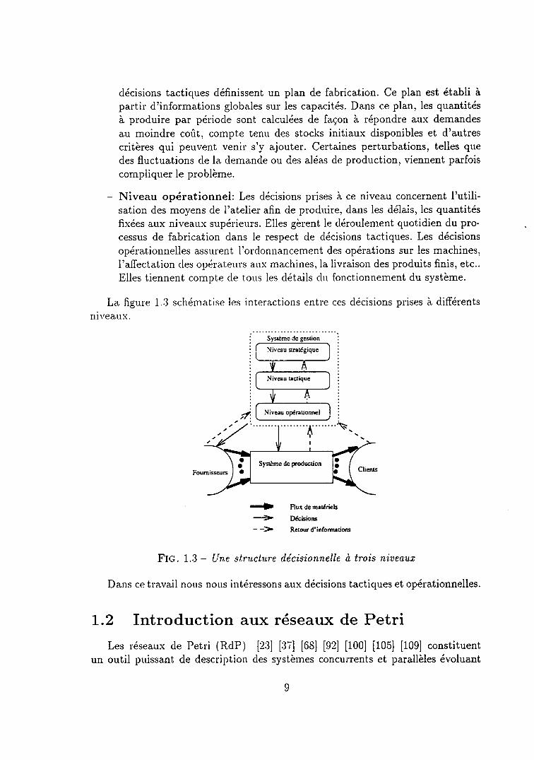
décisions tactiques définissent un plan de fabrication. Ce plan est établi àpartil d'informations globales sur les capacités. Dans ce plan, les quantitésà produire par période sont calculées de façon à répondre aux demandesau moindre coût, compte tenu des stocks initiaux disponibles et d'autrescritères qui peuvent venir s'y ajouter. Certaines perturbations, telles quedes fluctuations de la demande ou des aléas de production, viennent parfoiscompliquer le problème.
- Niveau opérationnel: Les clécisions prises à ce niveau concernent I'utili-sation des mo5'ens de I'atelier afin de produire. dans les délais, les quantitésfixées aux niveaux supérienrs. Elles gèrent le déroulement quotidien du pro-cessus de fabrication clans le respect de décisions tactiques. Les décisionsopérationnelles assur-ent I'ordonna,ncement des opérations sur les machines,l'affectation des opérateurs aux machines, la livlaison des produits finis, etc..Elles tiennent compte cle tous les détails clu fonctionnement du s5'stème.
La figure 1.3 schématise les interactions entre ces clécisions prises à différentsnirreaux.
.-f, Hur de marériels-> DécÈions
Ftc. 1 .3 - Une structure décisionnelle à trois niaeaux
Dans ce travail nous nous intér'essons aux clécisions tactiques et opérationnelles.
L.2 Introduction aux réseaux de Petri
Les réseaux de Petli (RdP) [23] [3i] [68] [92] [100] [105] [109] constituentun outil puissant de descliption des systèmes concurrents et parallèles évoluant

dans le temps de façon discrète, déterministe ou stochastique. IIs permettent unemodélisation simple des sys6!6es de procluction à des fins d'analyse mathématiqueou de simulation. Pour la simulation, on utilise souvent des réseaux de Petri com-plexes et généralement pauvres en plopriétés mathématiques, comme par exempleles réseaux de Petri colorés ou à prédicats [68]. Pour I'analyse mathématique, desréseaux pius simples, mais riches en propriétés, comme par exemple les réseaux dePetri élémentaires, sont utilisés. Puisque notre étude concerne I'analyse mathéma-tique des systèmes cle ploduction. nous nous limiterons aux réseaux de Petriélémentaires.
L.z.L Notions de base
Un réseau de Petri est un glaphe biparti composé de deux types de sommets: lesplaces et les transitions. Des arcs relient les places aux transitions, ou les transitionsaux places. Un arc ne relie jamais deux sommets de même nature. Généralement,les places sont représentées par des cercles et les transitions par des rectangles (oudes barres). Chaque place peut contenir un ou plusieurc jetons, représentés pardes poinbs. Comme nous les verrons plus loin. ces jetons pelmettent de modéliserla dynamique du système. Le narquage d'un RdP est un vecteur à composantesentières positives ou nulles. et dont la dimension est égale au nombre de places. Lenè*" composante de ce \;ecteur représente le nombre de jeions qui figurent dansla place n du RdP.
Plus formellement. un réseau de Petli est un 5-tuple G : (P, 7,, F, VV' IVI1)ori:
- P est l'ensemble fini des places
- ? est I'ensemble fini des tra.nsitions
- F est I'ensemble fini des arcs reliant les places aux transitions et les transi-t i onsauxp laces . Fçe x? ) U (TxP)
- tV : F + N esl la tbnction poids att,achée aux alcs, ori N est I'ensemble desentiers naturels.
- IVIo : P -> N U {0i est le marquage initial.
No tonsqueT îP :4 .Le RdP sans son marquage est noté PN : (P, T, F, l l l ) . Donc G:
(P/{, Ms). Lorsque tous les poids des arcs sont égaux à 1, le RdP est dit or-dinaire. Si.4/o est lemarqua.ge init ial d'un RdP C-i, lvIob) est lenombrede jetons
contenus dans la place p de CJ à I'instant initial.Dans la suite, nous tttilisons les notations suivantes:
- 't est I'ensemble cles places d'entrée de la transition t, c'est-à-dire I'ensembledes places p telles clue (p, t) e F.
i;.-r;i,l:'
10

- f' est I'ensemble des places de sortie de la transition t, c'est-à-dire I'ensembledes places p telles que (t, p) e F.
- 'p est I'ensemble des transitions d'entrée de la place p, c'est-à-dire I'ensembledes transitions I telies que (t,p) e F.
- p' est I'ensemble des transitions de sortie de la place p, c'est-à-dire I'ensembledes transitions I telles eue (p, t) € F.
Une transition f € 7 est dite franchissable (ot tirable) pour un marquage Msi, quelque soit p € ' t , M(p) 2 tV(p,l). En d'autres termes, une transit ion estfranchissable si chacune de ses places d'entlée contient un nombre de jetons aumoins égal au poids de I'arc qui la relie à la transition. Une transition t peut êtretirée (on dit encore mise à feu ot franclzie) si elle est tirable.
Le franchissement ou Ia mise à feu d'une transition I consiste à:
- retirer I,V(p,t) jetons cle chaque place p € 't,
- a joute l W(t ,p) je tons c lans toutes les p laces p € / ' .
Ainsi, à partir du marcluage l'1. le franchissernent d'une transition f conduitau nouveau narquage il,1' cléfini comme suit:
Nous noterons NIlt > ^,1'le fi'anchissement de f qui transforme IVI en t!/'. Nousnoterons aussi M[l > le fait clue t est fi'anchissable pour le marquage fu[.
A partir des notions cléfrnies pr'écédemment. il est clair que le marquage peutévoluer par tirs successifs cle tlansitions. On dira alors que la séquence de transi-t ions o: (f l , t ' , . . ' , f") est fra'nch.issable poul le marquage fuIo si les marquagessuccessi fs (Mt , I [2 , . . . , fu [ ' ) vér i f ient
ù Ik - r1 t k > À , I k pou r ,b = 1 ,2 , . . . , s
Nous noterons en abrégé I'lofo > 1\'1" pour signifier que M" est le marquageatteint à partir de l}/o par le franchissement de la séquence o.
Etant donné deux marquages M et .&/', nous dirons qr:,e M' est accessibleà partir de M si il existe une sécluence franchissable a telle que Mlo > M'.
L'ensemble de tous les marquages accessibles à partir de tI sera noté R(M).A partir d'une sécluence de transitions o, on peut construire un vecteur â,
appelé aecteur de com,ptage de la séquence, dont la. jième composante représentele nombre d'occurrences de la transition t; dans a.
( Iut(p) - tV(p,t) si p €. 't
Vpe P , À , I t (p ) : \ i \ t (p )+W( t ,p ) s i pe t ' (1 .1 )
L ,lz(p) sinon
i l

Si la séquerLce o est franchissable, le marquage fu[' atteint à partir de M par
le tir de a vérifie Ia relation algébrique suivante:
fu [ ' : fu [+Cxa ( 1 .2)
C'est, I' équation fondamentale ov,l' équatio'n d'état du réseau de Petri. Rappe-lons que C = lc;i l , i = l, 2, ..., lPl, i : !, 2, ..., l?l est la matrice d'incidencedu réseau. définie de la manière suivante:
(1 .3)
Notons que l'écluation 1.2 permet de calculer simplement le marquage atteint
pal une séquence a cluelconclue. sans c1u'il soit possible pour autant d'en déduire
si la séquence o est effectivement tirable. Par ailleuls le vecteur de comptage a ne
donne pas I'ordre clans lecptel les transitions sont birées'
Définit ion 1.1 (graphe d'événements) Lln grnph,e r l 'érénernents est un RdP
élémentaire dans lequel:
(i) chaqtte place u etu,ctentent une h'ansition d'entrée et u,ne transition de 'sortie;
(ii) tous les arcs sont pondérés à 1.
Définit ion L.2 (Tbansit ions sources et transit ions puits) Une transit ion
sans place d'entrée est ap7telée tra.nsition source. Ùn,e telle transition est toujou'rs
tirable. (Jne transition san.s place de sortie est appelée transition puits. Une telle
transition peu,t être tirée si elle est tirable. Si une telle transition est tirée, lesjetons sont préleués dan-* la (Ies) place(s) d'entrée suiuant les règles habituelles,
rnais aucun jeton n'est produit en sortie.
Nous verrons ultérieurement3 qu'une transition source est souvent utilisée,
dans un modèle d'atelier', pour modéliser I'entrée des matières premières (ou desproduits semi-finis) dans le système. De même, une transition puits est souvent
utilisée pour modéliser la sortie de produits finis (ou de produits semi-finis) du
système.
Déf in i t ion 1.3 (T- invar iant ) UnlT lxL aecteury te l que 9 i € NU{0} ,et y +0,pou r i : I , 2 , . . . , 1? l es t a2 t l t e lé un T - inua r ian t (ou T -se rn i - f l ' o t ) s iC xA :0 où
C est la matrice t l ' incidence.
( W(t ; , p ; ) s i ( f j , p ; ) e FÇ;j =
\ - l \ i (p;, t1) r i (po, t i) e P
[ 0 sinon
3 Voir chapitre .[ et annexe Cl
T2

Remarquons que, dans I'ensemble des T-invariants, si une composante donnée
est nulle, cela signifie qu'il n'est pas possible de revenir au marquage initial en
franchissant une séquence contenant la transition correspondant à cette compo-
sante. Dans le cas d'un atelier, cette situation signifie que l'état initial, qui peut
être par exemple un état nécessaire à une mise au point ou à un réglage, ne pourrajamais être retrouvé si I'on effectue certaines opérations. Il y aurait, dans ce cas'
une erreur de conception [105].
Définition 1.4 (T-invariant minimal) Lrz T-inuariant minimal est un T-
inaariant y tel qu, ' i l n'existe pas un T' inuariant x tel que x 1 y.
Un T-invariant minimal correspond à une gamme de fabrication. Utiiiser un
T-invariant qui est une combinaison linéaire de T-invariants minimaux revient à
décider d'utiliser différentes gammes dans des ploportions données ou, en d'autres
termes, de prendre a ltriori une partie des décisions de gestion [105].
Définit ion 1.5 (support de T-invariant) Soit y un T-inaariant. L'ensernble
llyll - {tl yltl > 0} des transitions est appelé le strpltort du T-in''uat'iant y, o'ù yltl
est la coordo'nnée tle y cott'es1ton.dant à lu transitiott t-
Définit ion 1.6 (support minimal) Soit u un T-ino-ur' i t t t t t . Son .support l lyl l e-*t
d,it minimut si llyll ne. contient pos ( uu sens strict ) de .sup2torts d'autres T-
inaariants.
Définit ion 1.7 (T-invariant à support minimal) UnT-inaarianty correspon-
d,ant à un support minimal est appelé un T-inuariant à support minintal.
Définition 1.8 (consistance) Un RdP G est d,it consistant si il existe un n'Lar-
quo,ge initial NIs et une séquence tle transitions francltissables o qui contient chaque
transition au moins une fois et tlont le franchi.ssement conduit à nouueau au tnar-
quo.ge initial NIs, i.e.. ùIslo > A,'Io et o ) 0. Il a été d.émontré que G est consistant
si et seule'rnent si il existe un T-inaariant strictement Ttositif pour G.
La consistance est une propriété structurellea liée à la réversibilité et aux états
d'accueils. Elle caractérise I'existence d'une séquence de transitions qui ramène le
marquage d'un RdP réversible au marquage initial.
Définition 1.9 (réversibilité) Un RdP G est dit réuersible si l'on peut toujours
reaenir au rno,rquage initial quelque soit le marquage atteint. i.e., NIs €. R(M)
pour tout tuI e R(Ms).a' Les propriétés structurelles ne dépendent que de la structure du RdP, et non de la manrère
dont les jetons évoluent dans le réseau. En termes de production, les propriétés structurelles
{épendent de I 'architecture du s,r-stème, et non de la manière dont i l est géré. On comprend I' im-
portance des propriétés structurelles lorsqu'on conçoit un système: elles permettent de garantir
des comportements ultérieurs indépendamment de la manière dont le système sera géré, laquelle
n'est pas connue à ce moment là.5'Un marquage M d'un RdP G est dit élal d'accaeilsi i l peut être atteint à partir de tous
les marquages atteignables, i.e., ̂ 4 e n(lul ') quelque soit M' e R(futo).
- r !
13

La réversibiiité est une propriété compormentale6, qui caractérise la possibilité
de relancer un système soumis à panne, après avoir solutionné des dysfonctionne-
ments.
Définition 1.10 (vivacité) Un RdP G est dit uiuant si chacune de ses transi'
tions est aiuante. (J'ne transitiotz t d'un RdP G est dite uiuante si elle peut être
franchie quel que soit le marqut.ge attei'nt, i.e..VX't e R(^'Io), llUI' €. R(M) tel
que t soit franchissable pour ArI''
La vivacité est aussi une propliété compoltementale. Dans un système de pro-
cluction, il est fréquenl clue des activités manufacburières se déroulent en parallèle.
Cela exige la synchronisabion de ces activités et le partage des ressources. Une mau-
vaise synchronisation et un paltage inadapté des ressoulces conduiseut non seule-
ment à une utilisation inefficace du système, mais peuvent également se traduire
par un blocage total ou partiel cles activités. L'étude de la tivacité d'un modèle
de RdP garantit I'absence cle blocage clans le système cle production considéré.
Définit ion 1.11 (bornitude) Lin.e place p de Ci est dite k-bo'mée si le nombre
d,e jetons dans cette l t loce ne rlépus.se jamai.s k. i .e. ' ùI(7t1 S k, VNI e R(^'Io).
[Jne place p r le G est d,i te bornée .si. el le est k-bornée pour un certain nombre
ent ier k > 0.G est dit le-borné.si le no'm,bre tle jeton-q dan.s chaque place ne dépasse pas k,
i .e., M(p) 1 lc, Vp e P et VM € Â(n1o). Autrentent dit, G est dit k-borné si
chaque place de G est k-bornée.Un RdP G est dit borné s'il est k-borné pour u,n ce'rtain nombre entier k > 0.
un RdPG est ditsain s' i l est l-borné. i .e., Ùl(p) S 1, vp e P etvI,I e R(ÙIo).
Certaines places d'un RdP. modèle d'un s.vstème de fabrication, représentent
des zones de stockage. D'autres places contiennent des jebons qui représentent des
ressources de fabrication. Il est souvent souhaitable de savoir si le nombre de jetons
dans ces places est limité: cela permet de dimensionner le système de production
correspondant, ou de découvrir certaines erreurs de conception. Par exemple, si un
modèle n'est pas borné, on pourra voir s'accumuler des en-cours dans le système de
fabrication correspondant, ce qui bien entendu n'est pas le reflet d'une conception
efficace dans le cas d'un système automatisé.Pour être complet, nous donnons la cléfinition d'un P-invariant qui est symétrique
à la notion de T-invariant:
Définit ion 1.12 (P-invariant) t ln lPl x I uecteur æ tel que t i € N U {0}, et
t *0 , pou r i : L ,2 , " ' , lP l es t a \ t \ t e lé P - inua r ian t (ou P -sen t ' i - f l o t ) s i x ' xC =0
où nt est Ia transposée dtL aecteur x et C est ln matrice d'incidence.
6' Les propriétés compormentales sonb souvent difficiles à étudier. Par contre, la plupart des
propriétés structurelles peuvent être aisément vérifiées à I'aide des techniques algébriques. Sous
certaines conditions, des propriétés structurelles irnpliquent des propriétés compormentales.
1.1

' irt ::
Nous aurons aussi besoin de la notion suivante:
Définition 1.13 (Conflit) Deur transitions fi et t2 sont en confl,it structurelsi elles o'nt au moins une place cornrnune en entrée, i.e', 't1î' tz * 0. EIIes
sont en confl,it effectif 'po'ur un rnarquo,ge NI si, d'e plus: AIIIL >, IuIlt2 > et
lp t.q. IUI(p) < W(p,t1) *W(p,t2). Un confl, i t effecti f correspond à un choio
exclusif entre deur franchissements.
L.2.2 Méthodes d'analyse générales
Arbres des marquages atteignables et arbre de recouvrement:[100]
[105] [e2] [1oe]Soit G un RdP muni d'un ma,r'cluage initial ffi. L'objectif de I'arbre des mar-
quages atteignables est de découvrir tous les marquages que I'on peut atteindre
à partir de ùIo. Un arbre des marcluages atteignables est une aborescence dontles nceuds sont les marqua,ges atteignables à pa.rtir de ffi, et dont chaque arcreprésente le tirage cl'une transition. La racine cle I'aborescence représente ù/s.
Notons clue chaclte mal'clua,ge concluit à a.utant de mat'quages qu'il y a detransitions tirables à par'lir ck: ce nlarcllra,ge. et clue Ie mêrne marquage peut se
retrour;er à cliffér'ents enclroit,s cle l'abolescence. Notons égalernent qu'un arbre desmar-quages atteignables se clér'eloppe incléfiniment clans la plupalb des cas.
Pour éviter d'aboutir à un ar'bre clui se développe indéfrniment, il a été décidé:
(i) qu'un marquage qui a été précéclemment rencontré est marqué par "old"1 unnæud marqué "old" sera ttne feuille cle I'aborescence;
(ii) que si un marcluage I/* obtenu est tel c1u'il existe. sul le chemin qui mène dela racine NIoà I,I-, un malquage A'I tel clue NI-(p)>- fvI@) pour toutes lesplaces p du RdP, et si :1.1-(p) > lul(p) pour au moins une place, alors le mar-quage de cette place est ma,rclué " o" (,i peut se comprendre comme signifiantI'infini). Ce marclua,ge restera i; dans tous les développements suivants, et larègle (i) s'appliclue égalernent aux malquages contenant le symbole c..'. Bienentendu, u I k : u)1 (t - k - rr.,, cluelclue soit I'entier É.
Un arbre de recouarernent est un arbre des marquages atteignables ajoutantles règles suivantes aux règles (i) et (ii):
(iii) un næud correspondant à un marquage tel qu'aucune transition n'est tirablesera marqué "DeadEnd" et constituera une feuille de I'aborescence;
(iv) tous les næuds clui ne sont pas marclués "old" et qui admettent au moins undescendant sont ma,r'c1tté "neiv".
L'arbre de recouvrement contient moins cl'informations que I'arbre des mar-quages atteignables, mais reste de taille limitée. L'arbre des marquages attei-gnables et I'arbre de recouvrement sont donc des outils d'analyse des RdP.
Ë 1 l l ' ' :
t5

- -.s".-+'.,
Les conclusions suivantes peuvent être tirées cle I'arbre de recouvrement et deI'arbre cles marquages atteignables:
- Un RdP est borné si et seulement si allcun des marquages correspondant auxnceuds de I'a,r'bre de recouvrement ne contient le symbole c.r. On comprendque si un RdP moclélise un système de production, il est nécessaire d'iden-tifier les situations clui augmentent les marquages indéfiniment. L'arbre derecouvrement est un moyen de détectel ces situations.
- L'arbre de recou'vrement permet de détecter les transitions qui ne sont pastirées, ou qui ne sont plus tirées à partir d'un certain point d'évolution. Celapermet de rnettle en ér'iclence les fonctionnalités d'un système de productionqui ne sont pas actives. ou clui cleviennent inactives att bout d'un certaintemps, pour certains é[ats initiaux du s,',*stème et certaines séquences dedécisions.
- Lolsclue le sysgi*" est borné. I'arbre des ma.rcluages atteignables donne I'en-semble des états clui peuvent être atteints les nns à. partir des autres, et larnanière cle réaliser ces transtbrma,tions. Du point cle vue des systèmes deplocluction, I 'alble cles états atteigna.bies foulnit clonc toutes les évolutionspossibles clu système connaissant son état initial .-eprésenté par i,Is.
Matr ice d ' inc idence et équat ion d 'é tat [100] [105] [92] [109]La matrice d'incidence d'un RdP est cléfinie pal la lelation 1.3 et l'équation
d'état est donnée pal l 'écluation 1.2.IJne colonne de la. matrice cl'incidence colrespond aux modifications apportées
aux pla.ces lors du fra,nchissement de la transition correspondante. ]Vlais la ma-trice d'incidence est indépenclante clu marcluage. Elle ne nous donne donc aucunlenseignement sur la possibilité de fi'anchir une transition donnée.
L'écluation d'état clonnée en 1.2 ne galantit pas que o soit tirable. Elle permet
simplement de trouver le marcluage atteint lorsqu'on connaît le marquage initialNIo et la séquence tirable a.
Il n'est pas possible cle représenter une boucle dans une matrice d'incidencecar cela exigerait dê mettre à I'intersection de la ligne correspondant à la placeet de la colonne corresponclant à la transition concernée par cette boucle à la fois
*1 et -1. Pour modélisel le fait que plusieuls opérations ne peuvent se déroulersimultanément sur la même machine, nous attacherons une boucle à toute tran-sition clans les modèles des systèmes de production comportant des transitionstemporisées. Cela ne nous empêchera pas d'utiliser la matrice d'incidence danstout calcul ne faisant pas intervenir le temps.
Méthodes de réducrion [100] [105] [92] [109]Un des problèmes que I'on rencontre lorsque I'on utilise les RdP pour modéliser
et analyser les systèmes cle ploduction est la taille généralement importante desmodèles obtenus (voir chapitre 3).
I O

Le tableau 1.2 résume les méthodes de réduction qui agissent localement sur
le modèle [105]. Elles sont de deux types, à sar.'oir les méthodes de transforrnation
et /es 'méth,odes tle sy'nth,èse .
IVIéthodes cletra,nsfbrtna,tion
sur lesplaces
simplification desplaces redondantesfusion de placesdoubléesfusion de placeséquivalentessuppresslon oeplaces impl ic i tes
sul les
transibions
post-fusionfusion latérale
pte-luslon
Techuiclues cle
synthèse
technicluesa.scendantes
combinaisou cleplacescornDlnarsoll de
chemins élémentailes
technicluesclescenclantes
affinage des
transitionsaflinage des places
Ti\B. 1.2 - fu[étlt,odes de réduction
Une place redondante est une place donb le marcluage n'influence pas le tirage
de ses transitions de sortie. Dans la praticlue, le marquage d'une telle place est lié
aux marquages des places clui ont les mêmes transitions de sortie.
Deux places h et pz sont structurellement doublées et peuvent être fusionnées
si aucun jeton n'arrive dans p1, p2 avant qu'un jeton ne soit arrivé dans chacunedes places des 't, où les transitions f sont les éléments de pi, qti.
Deux places h eL pz sont équivalentes si et seulement si il existe deux transi-
tions t1 et t2 telles que les conditions suivantes sont vérifiées: (i) P; (i : 1,2) est
une place d'entrée de t;, (ii) po (i : 1,2) n'est pas une place d'entrée de t3-;, (iii)
h et pz ne sont places d'entrée d'aucune autre transition que t1 et t2, (iv) t1 et
t2 ont mêmes places d'entrée et de sortie, excepté Pour ce qui concerne p' et p2,
ou n'ont pas de place d'entrée ou de sortie, (u) pr et p2 sont places de sortie d'au
moins une transit ion. Cette tra,nsit ion n'est pas nécessa,irement la même pour les
deux places.Une place implicite est une place clont le marquage n'est jamais un obstacle au
franchissement des transitions clont elle est place d'entrée, c'est-à-dire que lorsque
les autres places entrées d'une telle transition ont un marquage suffisant pour
. : ; " i , , 1 : ! i i . , r : r , !
: , . . - . r , i : . : : t t r l
-,.':.:.t.t
L7

permettre le franchissement, alors le marquage de la place considérée est lui aussi
toujours suffisant pour pelmettre ce franchissement.Les méthodes de transfbrmation partent cl'un réseau de Petri de taille impor-
tante, appliquent les règles cle transformation pour obtenir un réseau de faible
taille, et déduisent les propriétés du réseau initial des propriétés du réseau de
faible taille. Les règles de transformation qui préservent les propriétés souhaitées
ont été proposées dans [14], [80], [81]. L'inconvénient de ces méthodes réside dans
la difficulté que I'on renconble poul déterminel les sous-réseaux réductibles.
Les méthodes de s-vnthèse construisent les modèles RdP de manière
systématique et progressive afin de préselvel les plopriébés souhaitées tout au
long du processus cle conception. L'iclée est d'adopter un processus de conception
qui préserve les propriétés au lieu cle vérifiel les propriétés après avoir obtenu le
modèle RclP. Deux t1'pes cl'apploches existent: les méthode.s a-scendantes et les
m éth o d e s d e s cen d ant e -s.Une méthode descenda,nte palt d'un moclèle agrégé du système global, et I'af-
fine progressivement pour intloduire de plus en plus de détails. L'affinement prin-
cipal est de substituer- nn r'éseaux cle Petri bien formé à une place ou transition(voir, e.g., I t22], [126]. [132]). Cerre approche est bien adaptée pour modéliser les
systèmes composés cle sons-s-r'stèmes presque indépendants. Pour les systèmes de
production composés cle sous-svstèmes fortement liés à catlse de ressources par-
tagées, il est difficiie de trottr;er des modèles agr-égés de taille acceptable.
Une approche ascendante part des modèles des sous-systèmes (aussi appelés
modules) et intègre des moclules par fusion de places ou de transitions communes(voir, e.g., [2], [5] [i2] [95j [116] [132] ). Pour les approches ascendantes générales,
la faiblesse provient cle la. clifi[culté cle déterminer les conditions dans lesquelles
l'intégration préserve les propriétés souha.itées. Les approches modttlaires et les
approches incrémentales [28] sont éga.lement des approches ascendantes.IVIême si les méthodes cle réduction biennent une place non négligeable dans Ia
théorie des RdP et si elles s'a.pplicluent a.ux RdP dans lescluels les transitions ne
sont pas temporisées, elles exigent, dans le cas des RdP temporisés, des conditions
supplémentaires qui ne sont que très rarement vérifiées en pratique. C'est la raisonpour laquelle nous proposons plus loin une approche modulaire (voir chapitre 4),
qui est beaucoup plus naturelle clans I'industrie, pour résoudre les problèmes liés
à la taille. Nous verrons c1u'il est possible, pour certaines applications et sous cer-
taines hypothèses, de diviser le système à étuclier en modules de taille raisonnable,
de simplifier ces modules, puis d'en faire la synthèse d'une manière qui permet de
déduire les propriétés du s]'stème complet des propriétés des modules'
L.2.3 Réseaux de Petri ternporisés
Dans la littérature, on trottve trois types de temporisations:
- la temporisation des transit ions;
18

- la temporisation cles places;
- la temporisation de certains arcs
Ramchanclani [108] fut le premier à intlocluire les réseaux de Petri tempo-
risés. Dans son modèle appelé RdP T-tempolisés, il associe une durée à chaquefranchissement de transition. Dans le cas du modèle étudié par Sifakis [119], latemporisation est associée aux places et non aux bransitions. Ces réseaux sont
appelés réseaux P-temporisés eb, dans ce cas, les jetons ont un temps de séjourminimal dans chaque place. Stark [121] et Hanisch [51] ont proposés une autre
approche pour la prise en compte du temps: la temporisation est associée à cer-
tains arcs, appelés "alc temporisés". Les réseaux de Petri "arc temporisés" sont
utilisés poul mocléliser et anall-sel cer-tains pl'ocessus chimiclues [52]. Nous nous
intéressons aux processus discrets. Comme I 'a montré Sifal i is [119], les modèles deRdP T-temporisés eh cle RclP P-tempolisés sont écluivalents. Dans la suite, nouspréférons ubiliser la tempolisa,tion cles bla,nsitions cpri nous semble plus parlante
lorsqu' i l s 'agit d'activibés cle fabrication.Supposons clue le temps associé à, une transition t soit d1, et que le franchisse-
ment cle I débute à I ' instant 70. Alors. franchir la transit ion I consiste à:
1. r 'et irer VIr@,t) jetons cle tout p e' t ( i .e., cle toubes les places d'entrée de t)à I ' instant ?s;
2. ajouter W(t,p) jetons da,ns tout p € t '( i .e.. clans toutes les places de sort iecle t) à I ' instant To * 0t.
Entle les instanbs ?o et % * gr, les jetons sont supposés séjourner dans la tran-
sition. Cela leprésente. dans nobre approche, Ie séjour de pièces sur une machineau cours de leur transformation ou de leur assemblage. Cependant, les propriétés
des réseaux de Petri s'énoncent en supposant que les jetons concernés par un fran-chissement font partie des places d'entrée tant que le franchissement n'est pas
terminé.
1.3 L'approche proposée
Lorsqtre les demandes clui s'appliquent à un système de production varient au
cours du temps, nous disons que le système est à fonctionnement non cyclique. Lesperformances d'un tel systèrne dépendent de sa gestion, i.e., de la planification etde I'ordonnancement de Ia production. Les systèmes à fonctionnement non cycliquene peuvent plus être moclélisés à I'aide de graphes d'événements [105] [130].
L'approche que nous adoptons pour l'étucle des systèmes à, fonctionnement non
cyclique est modulaire et hiér'alchiclue [5a] [105] [i30].
: . : ! i .
19

l . - .. .iiË---,i..: r:. -,:L. . + -c.--'i5-giia ;^:i_,=::s-;_::fEfu;ir"g.qr. n*r,, .
. . . + : r . " t s . - : * q + . * i ! + . : * É t + _ : . . , , - . , , . . - - , l t r
s q j r r
: " d ' " : " : r
Pour modéliser et analyser un système de production réel, qui est souventcomplexe, nous adoptons une approche modula.ire (cf. chapitre 4 eI annexe C) qui
consiste à:
1. Décomposer le système de production en un ensemble de modules de faibletaille permettant une moclélisation et une analyse simple et efficace;
2. Modéliser les modules à I'aide des réseaux de Petri;
3. Analysel les propriétés qualitatives souhaitées pour les systèmes de produc-tion (bornitucle. vivacité, réversibilité. consistance, flexibilité, etc.);
4. Evaluer les propriétés cluantita.tives cle chacpe moclule (productivité, tauxd'utilisation des lessour-ces. niveaux moyens des stocks, etc.). Cette étapecomprend la conception d'un sy,'stème local d'aide à la clécision;
5. Intégrer les modèles cles modules de manières à pr-éselver les propriétés qua-l i tat ives souhaibées:
6. Déduire les plopriétés cluantita,tives du svstème intégré cle celles des modules.
En praticlue, le découpage cl'un s-r'stème cle procluction en modules dépend dusystème considéré. Il peut êtle r'ésolu par une approche combinant I'expertise etles techniques de classification automaticlue [105].
L'ut i l isabion d'une apploche modulaire nécessite des:
- transitio'ns d'entréÉ. poul représentel I'arlir,ée cle produits ou de matièrespremières dans un module:
- transitions de sortie, pour représenter le départ de produits finis du module;
- places d'interfuce, pour relier les clifférents moclules.
Pour gérer le système, nous adoptons I'approche hiérarchique qui comprendune hiérarchie à deux niveaux. Dans le prochain chapitre (chapitre 2), nous mon-trerons les avantages et les inconvénients de I'approche hiérarchique en étudiant laplanification d'un système de production simple. Comme un outil complet, RdPsera utilisé. dans les chapitres suivants, pour la moclélisation modulaire et la ges-tion hiér'archique de systèrnes de procluction discrets.
20

Chapitre 2
Une hiérarchie à deux nlveaux
2.t Approche hiérarchique et approche globale
Les s_vstèmes de procluction classiclues sont généralement de taille importante,ce qui rencl leul gest,ion courplexe. En planifica.tion cle la procluction, on distinguedeux approches fonclamentalement cliffér'entes: I'approche globale et I'approchehiérarchique.
2.L.L Approche globale
Cette approche utilise un moclèle rnonolithique clui cléclit le problème de plani-fication de manière détaillée. Elle foumit toubes les décisions sur I'horizon complet.
L'approche globale est lrès l imitée pout' les ra,isons suivantes:
- Le ploblème de pla.nifica,lion est coularnment formulé comme un problème deprogrammation linéa.ire en variables mixtes. Les procédures par séparationet évaluation, clui utilise parfois la technique de relaxation lagrangienne pourIe calcul des bornes inférieures, sont souvent mises en ceuvre pour obtenirla solution exacte [69]. Ces procédures sont souvent inacceptables en raisond'un temps de calcul exponentiel. Des méthodes approximatives basées surdes techniques de clécomposition sont proposées [75], mais ne garantissentpas I 'obtention d'une solution admissible.
- Beaucoup de clonnées sont prévisionnelles, ce clui conduit à des résultatssujets à caution lorsclu'on fait cles prévisions détaillées sur un horizon im-portant.
21

. _ r " - . . r A . . : _ : . ' , ' . ? à i 4 . 4 r ' . ' * È : ' . . : _ . : r " i J ' 1 : - _ '
..,]--î, i"" ' . ' ' i";Ff; '+"i -: '-: ' ;-": ' l . ' : '
2.L.2 Approche hiérarchique
L'approche hiérarchiclue est proposée par de nombreux auteurs l. Cette ap-
proche décompose le problème de planification en sous-problèmes. Chaque sous-
problème est lié à un niveau cle la hiérarchie. A chaque niveau, les entités sont
des agrégats des entités clu niveau immédiatement inférieur. L'horizon de planifi-
cation décroît en descendant dans la hiérarchie. Les décisions correspondant à ces
agrégats sont désagrégées au niveau immédiatement inférieur.Plusieurs efforts ont été fait dans le domaine de la gestion hiérarchisée de
systèmes de production. \ ioir e.g., [19], [20], [16], [39], [18], [50i, [ l ] , [17] ' [110]'
[93]. Plusieurs modèles ont été étudié, e.g., le modèle de Hax et Meal [57], le
modèle de Axaster t6] ti] [E], le modèle de Tsubone, Nlatsuura, et Tsutsu [125], le
rnoclèle de Saacl [112]. le moclèle cle Thompson, Davis et lVatanabe [12a] [123], le
modèle de Inman et Jones [67].Des synthèses de la littérature snl I'apploche hiérarchique de la production
peut être trouvées clans [42] [36] [91], ainsi clue clans les thèses de Xie[128], t\Ieier[90],
Nagi[93], Libosvar[S3], et N'[ehra[S9].Xie [12E], après a,r 'oir introcluit la notion cle configuration, a étudié I 'ordonnan-
cemenr en remps réel c['un atelier' flexible par une arpproche hiérarchique à trois
niveaux: sécluencement cle configurations, contr'ôle de flux et ordonnancement en
temps réel. La notion cle configulation a pour but de décrire un état du système
permettant de fablicger un ensemble cle procluits. Les machines de I'atelier sont
sujettes à pannes.lvleier [90] s'intéresse a,ux problèmes posés par la. gestion de production d'un
atelier flexible. Une procéclure hiér'archiclue à cleux niveaux a été développée pour
Ia planification et Ia. comma.ncle cle la ploduction.Nagi [93] a étudié la conception et I'exécution d'un système de gestion de
production hierarchisée. L'agréga.tion spatiale et temporelle, la consistance et la
désagrégation sont étucliées.Libosvar [83] s'intéresse à la gestion des flux de production. Ce type de décisions
est à prendre au niveau le plus élevé d'un système de gestion de production
hiératchisée.Mehra [89] a proposé une méthode hiérarchique à deux niveaux pour aborder le
problème de planification cl'un s.n*stème de production. L'agrégation des produits,
I'agrégation des machines et I'agrégation du temps sont considérés simultanément.
Cette méthocles a été applicluée à un atelier de Pungborn Corporaffoz (USA).
Afin d'introduire les bases de I'approche hiérarchique, nous étudions, dans ce
chapitre, Ia planification cl'un sy'stème de production simple. L'objectif est de
montrer comment la valeur de la fonction objectif varie avec le coût de stockage
des produits dans la cellule, ce clui permet de se faire une idée des avantages et
des inconvénients de I'approche hiérarchique.
r voire.c.,[6] t7l t8l tel [r0] [16] [1i] [1e] 12011221[84] [36] [3e] [40] [4211431[50] [53] l57ll77l[82] [87] [e4] [110] [111] [112] [123] [124] [125] [12i] [131] [135] [8e] [e0] [e3] [128] [E3]
22

2.2 LJn exemple illustratif
Considérons un système à 2 machines l}11 et IV[2 qui fabrique 4 types de produits
Pt, Pz, P3, et P+. Ce s5'stème est illustré par la Figure 2.1'
p : €
pr -J
,, _I
P4 -
Ftc. 2.1 - Un exemltle
On fait les hypothèses suivantes:
1. A chaclue t5rpe cle plocluit esl a.ssocié un routage clui indique la sécluence des
machines à visitet pour effecttter sa fabrication.
2. Pour chaclue tr,pe cle procluit, , le clelniel stock est, ut i l isé poul stocker les
procluits f inis.
3. Un cofit de stockage et un coût de r-upture sont associés à chaque stock de
produits finis. On suppose que ces coûts sont déterministes et qu'ils sont
connus à priori. La rupture cle stock n'est pas autorisée pour les produits en
cours de fabrication.
4. La durée de chaclue opér'ation est déterministe et connue à priori.
5. Les matières plernièr'es arrivent dans le s-,,-stème sul' un mode "juste-à-temps".
Par. conséqtient. on peut supprimer les premiers stocks cle chaque type de
produit, et on obtient la Figure 2.2.
83 l
812
BT2
v2
H}
PI
u2
P4
Frc. 2.2 - Le système obtenu en su'pprimant les premiers stocks
23

I
2.3 Modélisation des systèmes généraux
Dans ce paragraphe. on généralise I'exemple précédent et on présente des
définitions supplémenbaires.
2.3.L Définitions et notatious
Nous uti l isons plusieuls cléf init ions:
1. Horizon: ' l l : Tt lJ Tz U ...U Tri- est une périocle de longuew I( x H.
,If es[ le nomble cle périocles élémentaires. ,[/ est la longueur de chaque
périocle élémentaire. Dans la suite, on suppose clue la durée de chaque période
élémentaire est la même. L'hodzon est I'extrémité de la période 'lf , c'est à
dire I'instant 1( x .É1 si I'instant initial est I'instatnt 0.
2. Machiles: M : {il.1r ,.tL/2," ' . r\1-}, nz est le nombi-e de machines considérées.
3. Types de produi ts : F - - {Pr ,Pr , " ' -P, } , r l est le noml l . . .e de types de
procluits consiclérés.
4. Stocks: IE = {Bti | fl r'isite i,Ij}. Bij est le stock dédié au produit 4 à la
soltie de la machine il,,l;. On a cleux ty'pes cle stocks: les stocks internes et
les stocks terminaux (i.e., stocks contenant des produits finis).
5 . Opéra t i ons : O : {< P ; , ) [ ; > l f , v i s i t e M i , ,V i : 1 , " . ' r ? ;V j : 1 ' " ' , r n ]
est I'ensemble des opéra.tions dans le s-\'stème.
Ponr chaclue i : 1." ' ,??, olt cléf init O; : {< P,,I ' l i >l 4 visite t\ I i ,Vj :
1,.. . ,m) comme I 'ensemble cles opérations nécessaire pour la production de P;.
Pour chaque j - 1 , " ' , nz , on dé f i n i t n i = {P ; IP , v i s i t e f u I1 ,Y i - l , ' " . , n }
comme I'ensemble cles t."*pes de produits qui visitent la machine NIi.
On définit aussi:
- Onre - { ( i , f ) l l " rang c le I 'opérat ion 1P; ,ù[1>€O; est in fér ieur à lO; l ]
- Olin - {( i , j) l l" rang de I 'opération 1 P;, ù11 >€ O; est égal à l{2; l}
On note 1P; , I ,11 )11 P; , i '11) poul s ign i f ier qr te I 'opérabion 1P; , fu f i ) est
suivie par I 'opération ( P;, À,11).Les paramètres sLrivants sont utilisés:
t;;: temps nécessait'e pout' exécutel I'opér-ation ( P;, À'Ii );
a;;: cofit de stockage associé aux stocks B;i €.IB, Vi' 7;
B;: coît de rupture associé aux stocl is Bij €.8, V(i ' j ) ,91;n,Vi-
2+

On note aussi d;(È) la demande de 4 à la fin de la période ?i,.Les variables d'état sont:
x;i(k): niveau du stock Bij à la fin de la période ?6.
Les variables de contrôle sont:
u;1(k): nombre de produits de type P; qui doivent subir I'opération < P;, Mi >durant la période 76.
2.3.2 Positionnement du problèrne général
Avec les notations précéclentes et les cleux notations conventionnelles suivantes:
ru+ : nzac (z ,0 ) x - : - r t t i r z (2 ,0 )
le problème de planification cle la production peut s'écrire comme suit:
IUI ;n l l { I a ; rx : ; ; ; (A) * t [oor rx l (k ) * l3 tx" ; (È) ] ] (2 .1)È t j l ( i . j )eOp" i l ( t . i )e o / ' "
sous les contraintes suivantes:
- dynamiclue d'état:
,o i (k)
vÀ, v(i. j) e or", (t. /) € oP,', 1 P;, À,11
q i ( k ) : x ; j ( k - 1 )+ t r ' ; i ( k ) - d ; (À ' ) , Vk , V ( i . j ) e O t ' " (2 .3 )
- contraintes de capacité:
t t ; i x u4(k) 1 H, Vi, Vki :P;e.X t
- contraintes sur les variables:
, , , , f 2 o, si k > o, v(i, i) e oo'"r ; j (k) t =r , r to l , s i f r :o r t - - (2 '5)
,, i(k - 1) 2 u;;(È) > 0, Vi, Vi, VÈ (2.6)
Le critère (2.1) signifie qtle la fonction objectif est de minimiser la somme descofits de stockage et des coûts de rupture sur I'horizon de planification.
Les contraintes cl'états clistinguent deux cas: stocks internes (2.2) et stocksterminaux (2.3) contenant les produits finis.
(2.4)
25

. ,.:..i'-..:r., :i, --';Jf-i.'r;':=1,.j:.1'*#iti1.'.=îrtri:,rr;ir,',-r*:;i;,::: . . . . . i - : . ; . ' , . * 1 ] ' . , ; F ' ' : : . . + . ' * . . ' , ' . . .
Les contraintes de capacité (2.a) indiquent que, pour chaque machine' la somme
des temps d'exécution des opérations prévues sur une période élémentaire ne doit
pas excéder la durée de cette pér'iode.Les contraintes (2.5) et (2.6) indiquent d'une part qu'il ne peut y avoir de
rupture dans les stocks internes, et d'autre palt que la production d'une machine
durant une période élémentaire ne peut excéder le contenu des stocks en amont
au début cle la période.
2.4 Modélisation du système il lustratif
2.4.L Ltexemple re-visité
Afin cle facilitel l'étude clu système illustr-atif, nous re-étiquetons tous les buf-
fers et nous étiquetons toutes les opérabions. ce clui est schématisé dans la Figure
2.3 dérivée de la FigLrrc 2.2.
Ftc. 2.3 - Notation-q déftnitiues
Ainsi, on a les paramètres suivanbs:
- t t , . . . , tor temps nécessai re pour exécuter les opérat ions Opl , " ' ,Op6;
- d t ( k ) , , . . . , da (k ) : demande de P r , " ' , P+ i
- cr (0) , . . . , 16(0) : n iveaux in i t iaux des s tocks Bt , " ' , Boi
- 0r , . . . ,9{ coûts c le rupture pour les types de produi ts Pr , " ' ,Pn dans les
s tocks B t , . . . , Bq i
- o1; . . . ,o6r coûts de s tockage des produi ts dans les s tocks Br , " ' rBu.
On a encore cles variables suivantes:
- a l k ) , . . . , r 6 (k ) : n i veau des s tocks B t , " ' ,Baà l a f i n de pé r iode k ;
- ur(È), . . . ,u6(le): nombre d'opérations Oqt|, ' ' ' ,Op6 exécutées durant la période
k .
D J
D T
B2
84
P:}
P I
Y2
J
26

2.4.2 Formulation du problème donné en exemple
Avec les paramètres et les variables précédents, on peut poser le problème
relatif à notre exemple. Il s'écrit:
K 6
MinD{La; x rf (fr) +10; x r '-(k)} (2 .7 )È=l i=1 r=-l
Sous les contlaintes (
- dynamique d'état:
c ; (k ) : t ; ( k - 1 ) + u ; (k ) - d ; (k ) ' i = 7 ,2 , ,3 ,4
.z:5(k) - t r (k - 1) + z5(fr) - zr( f r )
. r '6(Ë) : r 'o( f r - 1) * uo(Â') - u2(k)
- contlaintes de ca,pacité:
t1 r r1 (À: ) * t2 t r .2(k) * / . ru . r (À ) <
fuq(k) | t5 t t5(A) + t6u6(À' ) <
- contraintes sur les variables:
z ; (È ) : t ; ( 0 ) , 4 : 0 , i : L , " ' , 6
z5 (k ) Z 0
uo( f t ) 2 0
0 (u1 (k ) <c5 (k -1 )
0<u2 (k )<c6 (k -1 )
us (k ) , un (k ) ,u r (È ) ,u6 (È) > 0
H
H
(2 .8)
/ t o )
(2 .10)
(2 .1 1 )
(2.12)
(2 .13)
(2.r4)
(2 .15)
(2 .16)
(2.17)
(2.1s)
Dans ce cas spécific1ue, la fonction objectif (2.7) à minimiser est la somme des
cofits de stockage et des coûts cle rupture pour les 4 types de produits sur I'horizon
de planification.Les contraintes (2.8) à (2.18) ont été expliquées lorsque le problème général a
été introduit.
27

*;*;t*iî, .si*'s:; :1.1. : ":':*,'.f ;l. ffii*-t-sniî,,]î,,k.,:*,t,i
2.5 Le modèle du niveau haut
Au niveau haut, les 2 machines ùfi et Ù12 sont groupées en une cellule, et les 4
types de produits sont groupés en deux familles de produits: P1 et Pz sont dans la
famille Ft, Ps et Pa sont da,ns la famille -Fz. Cette situation est schématisée dans
la Figure 2.4.Sàient -[T nombre cle sous-périodes, È la longueur de chaque sous-période, donc,
Ii x H - I7 x II.Soient aussi
Tr, Tr les temps nécessaires estimés au niveau haut poul la production d'une
unité cle chacttne cles tâmilles 4 et ,F2 r'especbivement.
Dr(*), Dr(") les clernancles cles familles Fl et F2 respectivement à la fin de sous-
périocle rc.
Xr(0), Xr(0) les stocks init iaux ponr F1 et -F2 r 'espectivement'
Br, Fr les cofits de luptttre pour F1 et F2 r'espectivement.
at. dz les coirts cle stocliage Pottr Fl et F2 respectivemenb.
Xr(^), X2(,r,:) les nivea,ux cles stocks de F et F2 respectir;ement au début de Ia
sous-période rc.
Ur(*), Lrz@) Ies quantités cle F1 et F2 produites respectivement pendant la sous-
pér'iode rc.
On a besoins cle spécifiel les paramètres suivanbs afin cte gouvo]1 constlrire-le
modèledu n iveau haut :1î : FI ; Tr , Tz: Dr(^) . Dz(rc) ; Xr( t ) , Xr(n) ; 0 t , 0z;at , a2.
Une cles apploches dont on peut disposel pour évaluer ces paramètres se trouve
dans [58]. Pour le cas spécific1ue étudié, nous obtenons facilement:
( i ) / i : 30 , I i : 6 ; H :5xH .
Ftc. 2.4 - Nit;eau h.aut
rA
T1, U l
T2, U2
28

(ii) La demande de chaque famille pendant une sous-période est égale à la sommedes demandes de tous les types de procluits (qui appartiennent à la famille)pendant les périodes élémentaires de la sous-périodes:
Dr(*) : I {a , [5 x ( rc - 1) + i l+ d2 l5x ( rc - 1) +r ] ] ,; - 1
5
Dr(" ) : f {a [s x (n - 1 ) + t ] + d4 l5x (n : - 1 ) + j l ] ,t - 1
K : t r . . . , 6
Æ:1, . ' . , 6
( i i i ) n en est de même potrr les stocks init iaux:
' \ ' ( 0 ) : r r ( 0 ) *12 (0 )
X r (0 ) : r e (0 ) * r a (0 )
Il n'est pas possible cl'ér,aluer pr'écisément les paramètres B1, 9z; at a2, car. ilsdépendent des quantités cle chaclue type cle produit fabriquées, et ne peuvent doncêtre obtenus qu'après la résolution cltr problème de niveau bas qui donne les quan-tités cle plocluction r'éel de chaclue svpe de procluit. Dans [58] ces paramètres sontapproximés en consiclérant les mo-u-ennes ponclérées par les demandes de chaquetype de produits. Dans l'exemple aucluel nous nous intéressons, nous avons:
â _f) l -
B,:
0t xLu*=tDl,=rrlr[5 x (n - t)+ i]+ 0z x D|=r Dl=rdrlî x (rc - l) + tl
gz x D6*=t Dl=, d.[5 x (ru - 1) + i] I g.t x D1=, Dl= da lsx( rc -1) + iï=, I ' ,?=,{r / j [5 x (" - 1) + t ] + dalS x (rc - 1)+ i ] ]
qtri donne les corits cle ru1>tr.rle estimés pour les farnilles F1 et F2 respectivement,et
or x DÎ=r Dl= 5 x (rc - 1)+ i l* a2 x D|=r Dl=rdrl ï x (r - 1) +i l0 r =
d z =
l= , D ' ,?=, {d1[5 x (^ - 1) + i ] + d2 l5 x( ,c - 1) + i l ]aa x D|=r D;t=rd.[5 x (ru - t) + i] * oa x D1=, Dl=, da[5 x(rc - 1) +i
3=' Dl='{r /u[5 x (,c - 1) + ej + dq[S x (rc - t) +i ] ]
qui donne les cofrts de stockage estimés pour les familles F1 et F2 respectivement.Les temps de fabrica,tion pour les familles sont estimés dans [58] comme suit:
: f1 -mcrxp l lB l lx. mariç1,wetl ti,-
où z est le nombre cles périodes élémentaires dans une sous-période qui est,dans notre cas, [{ f Hi
ti,,u est le temps nécessaire pour exécuter I'opération ( PlrlVI- );
? t l
D1=, Di=, {d1[5 x (o - 1) + i ] + d2[b x( rc - t ) + i ] ]
29
rfo est le valeur à estimer, i.e., le temps nécessaire pour exécuter la qh'
opéra[ion cle la famille / durant la sous-période rc. Rr? est I'ensemble des ma-
chines qui effectuent la tf^" opération de la famille / aucluel Pi appartient. Dans
notre cas, nous avons:
5' 1 \ : , , , J xmax ( t1 , t 2 , t 5 , t 6 )' ) + r - -/
T2 : -+_ "xmax ( t s . t a )a+ r_ r
Après avoir évalué les paramètres précédents, on peut poser Ie problème au
niveau haut comme suit (cf. problème 2.1):
6 2
À,t inl { I [at x ê;(rc) * - i3;
x / ' (") ] ] (2.19)x = 1 r = l
sous l es con t ra in tes su i va ,n [es ( pou r t ou t x - 1 . " ' , 6 , i - 1 , " ' , 2 ) '
X ; (o ) - X i ( r : - 1 ) * L t ; (n ) - D ; ( ru ) ,)
Dtn xsi(K)\sF{,i = l
e; ( ru ) -X ; ( ru ) 20 ,
/ , (n : ) +X; ( r , ; ) )0 ,
U;(ru) ) Q,ë;(ru) ) 0,
/ '( ') > o,
2.6 Passage du niveau haut au niveau bas
Après avoir construit le modèle du niveau haut et avoir obtenu la planifi-
cation à ce niveau, on peut utiliser les résultats de cette planification comme
contraintes pour le problème du niveau bas. La planification (niveau haut) consiste
à déterminer la quantité de chaque famille fabriquée dans chaque cellule durant
chaque sous-périocle. Les clécisions prises au niveau bas concernent la production
de chaque type de produit sur chaque machine durant chaque période élémentaire.
Nous résolvons le problèrne du niveau bas en deux étapes: désagrégation des fa-rnilles, pvis désagrégatio'n temporelle et spatiale [58].
2.6.L Désagrégation des familles de produits
Puisque nous avons deux familles de produits, nous devons résoudre deux
problèmes de programmation linéaire poul effectuer cette désagrégation.
30

So i t y ; ( r c ) , i : L , . . . , 4 ; Æ: 1 , " ' , 6 , l a p ropo r t i on de p rodu i t s de t ype f ldans les familles Fr ou r.2 pendant la sous-période rc. On note aussi z;(le), i =
1, . . ' i ,c : 1, . . . , 6 le niveau du stock de produit P, à la fin de la sous-période rc.
Résoudre les deux problèrnes ci-dessous conduit à la détermination de y;(x),, i :
1 , . . . , 4 ; r c : 1 , " ' , 6 .
6 2
A/IinD{Dla; x e;(rc) * Ê; x /,(")l}*=l i= l
sous l es con t ra in tes su i van tes (pou r t ou t r c - 1 , " ' , 6 , i : 1 ,2 ) :
(2.20)
5
r r ( rc ) : r r ( rc - 1 )+ y1( r , : ) x Ur@) -Ld t (5 x ( rc - 1 ) + j )
' r ( r ) =æe(rc- l )+ue( rc) x UzG)- iar f tx ( rc -1) + j )
a. t (n ) = x , t (n - 1 ) + y . r ( r r ) x u r ( * ) -Lan6 x ( rc - 1 ) + j )i = l
J = 1
5
(2.22)
(2.23)
(2.24)
(2.25)
(2.26)
(2.27)
(2.28)
(2.2r)
(2.30)
* r ( * ) : xz(x . - 1) + uz(rc) x U ' ( " ) -Dar ! x ( " - 1) + i )l = l
v (n ) *uz (n ) : l
e ; (n ) 2 c ; ( ru )
. / , ( t ) > - " ; ( " )
y;(*) à o
e ; ( c ) ) 0
/,(rc) 2 o
L'objectif (2.20) consiste à minimiser la somme des coûts de stockage et derupture des produits P1 eT, P2 (qui appartiennent à la famill" Ft) sur I'horizon
de planification, i.e., sur 6 sous-périodes dans notre cas. Les contraintes (2.21) et(2.22) concernent les niveaux des stocks X1 et )(z relatifs à Pr et P2 respectivement.Les contraintes (2.23) indiquent que la somme des ratios de Pr et P2 dans Ia famille^Fr est égale à 1. Les inégalités (2.24) à (2.28) sont des contraintes introduites pour
transformer Ie problème initial en un problème de programmation linéaire.
6 4
Minl { I ["r x e;(rc) * 0; x / ,( ' ) ] ] (2.2s)x=l i=3
sous l es con t ra in tessu i van tes (pou r t ou t r c - 1 , ' ' , 6 , , i - 3 , ' " , 4 ) ,
; - 1
J
31
(2 .31)

i . , - . . . - . : : : " t : . : . " ' , . ; , ; : ; . : ' . . , . . . ' l l : : : ; i : i , i = i . . " " ; r : i i : i
ys (E )+9a ( r c )=1
e;(rc) > z;(rc)
i ( " ) 2 - "n (o )
vi(rc) 2 o
e;(rc) à o
/ ,(o) 2 o
Les problèmes (2.29) et (2.20) sont semblables. Le problème (2.29) concerne
Ies produits P3 et & et le ploblème (2.20) concerne les produits P1 et P2.
2.6.2 Désagrégation temporelle et spatiale
Après avoir obtenu la planification cle niveau haut et déterminé les ratios des
produits dans les fanrilles, nous pa,ssons à. la planificabion de niveau bas. L'objectif
est de déterminer la cluantité cle chaclue type de ploduit à fabriquer pendant chaque
période élémentaire sul les machines c1u'ils utilisent. La résolution du problème
condu i t à l a dé te rm ina t i on c les u ; ( l ) . i - - 1 . ' ' ' . 6 ; / : 1 . ' " . 30 .Le problème s'écrit :
(2.32)
(2.33)
(2.34)
(2.35)
(2.36)
(2.37)
x,I i t - t tx(Æ{)+5
{È *, * "r( j )
j = 5 x ( x - l ) { l t = l
sous les contraintes sttivantes ( potrl tottt ru : 1,
( o - 1 ) * 5 ) :
4
+l g; x / ,U)) (2.3s)t - l
" ' , 6 ; i : 5x ( rc -1 )+1 , " ' ,5x
r ; ( , r ) : r ; ( i - 1 )+ r r ; ( i ) - t l ; ( i ) , i : 7 ,2 ,3 ,4
, t ( j ) : r r ( j - 1 ) + us( r ) - " t ( j )
roU) : ,uU - 1 )+ uo( j ) -uz ( j )
t1 x u1$) * tz x "zU)
+ t t x ut( j ) 3 H
13 x u3( j ) * t5 x ur(r) *ro x uoff) S I /
5 x ( x - l ) * s
t u ; ( j ) : y ; (o) x t r ' (o) ,j = 5 x ( æ - 1 ) * 1
5 x ( x - r ) * 5
t u ; ( j ) : y ; (o ) x L iz (n ) ,j = 5 x ( r - l ) * 1
0<urU) Sr5 ( / -1 )
O<uz j )<zoU- l )
i : I ,2
i :3 ,4
(2.3e)
(2.40)
(2.4r)
(2.42)
(2.43)
(2.44)
(2.45)
(2.46)
(2.47)
32

fi,'.. ,iitril.* .*
ri "rri. :.- . . .: :
, . l : : ; ,11, i f . , ' i t : ) ' - . "-- ' : i r : : . : l . r i
us]) , ur( l ) , us( i ) ,uo(r) 2 0
eiu)> r ; ( r ) , i :1 , . ' . ,6
f ;U) 2 -r ;(r) ' i : 1 , . . . 1 4
Il s'agit ici (fonction objectif (2.3S)) de minimiser la somme des corits de
stockage et de rupture des produits Pr à Pa sur I'horizon de planification. Les
contraintes (2.39) à (2.41) concernent les stocks Br à Be. Les contraintes (2.42)
et (2.a3) sont les contraintes de capacité cies machines IVII et NIz respectivement.
Les contraintes (2.44) et (2.a5) sont les contraintes provenant du niveau haut. Les
contraintes (2.a6) à (2.50) sont intlocluites pour transformer le problème en un
problème de prograrnmation linéaire.
2.7 Résultats numériques
On a résolu les problèmes ptécédents à I'aide du logiciel OSL2.
2.7.L Valeurs des pararnètres
On choisit les valeurs cles para,mètt-es comme suit:
- 1{ - 30 est I'holizon de pla.nification contient 30 périodes élémentaires;
- H - 30 est la dur'ée cle chaque période élémentaire est de 30 unités de temps;
- les temps nécessa.ires ponï exécuter les opér'ation sont donnés dans le tableau
2 . I t
T,q,s .2.1 - Temps opératoires
- r;(0) = 10, i = I, . . ' ,6 sont les stocks init iaux. IIs sont tous égaux à 10.
2.7.2 Résultats et conclusions
On consiclère la demande de chaclue type de produit comme aléatoire. La loi
de distr.ibution uniforme, U[a, b], est applicluée à la demande. On désigne la valeur
moyenne cle cette distribution pal a. Selon la sélection des valeurs de a et ô, qui
2 OSL (Optimisation Subroulin,e Librarg) est un logiciel commercial de IBM. Yoir Optimisa'
lion Sçbroulin,e Librarg, Guide and Reference, Release 2, Third Edition, July 1991
(2.48)
(2.4e)
(2.50)
t1 t2 t3 ta t -v J t6
1.1 1 .3 1 .8 2.0 T,7 1 .4
33

sont respectivement les bornes inférieures et supérieures, les demandes peuvent
être générées afin que les machines travaillent en surcharge ou en sous-charge.
Dans les Figures 2.5 à2.9,Ia coordonnée horizontale représente la valeur des
paramètres û5 et o6 (on suppose eue û5: oo), la coordonnée verticalereprésente
la valeur prise par la fonction objectif. Les Figures 2.5 à 2.9 donnent des résultats
des cinq groupes d'essais.
r Figure 2.5:
- les corlts de stockage dans les stocks Brr'" , -Ba sont dr : ' ' ' : a4 :
10.- les demandes d1 ," ' ,d, pour les produi ts Pr," ' , Pa sont:
T,r,s. 2.2 - Es.sai I : Dem,anrles pour Pr," ' , Pu
! '
rY
r 00000
s 0 0 0 0
6 0 0 0 0
4 0000
2 0000
n
Legende:
250 300
Frc. 2.5 - Es.sai I
Approche hiérarchique
Appræhe monolithique
100 150 200
cr 5=cr 6
Figure 2.6:
- les coûts de s tockage dans Br , " ' ,Ba sont o1 : " ' - Q4:100.
- les demandes dr," ' ,do pour les produi ts Pr," ' ,Pa sont:
T,c.s. 2.3 - Essai I I : Demandes pour Pt," ' ,Pu
d1 d2 tlj d4
3.4 3 .1 3 .3 4.9
/ '
d1 d2 cls tla
3.4 3.4 3.3 4.9
34

I - - * . , 4 , i - à - - - : , L , . : . - r - - " - : j 5 : : , Ë è r , : d i i - , : . - : - , ; j - . r . . - r .
- : _ { \ i q r q r l
. . . i ' . . . . ' ' ' : , . . : ' ' . r J , . . ' ' - " ' ! . a ; . . j
o so too..
,t]I utoo
250 3oo
Flc. 2 .6 - Essai I I
o Figure 2.7:
- les coûts de stockage dans Bt," ' , Ba sont Qt : " ' - o4 : 10.
- les demandes ch.' ' ' , r /4 pour les produits Pr, ' ' ' . P.r sont:
Trs. 2 . .1 - Essai I I I : Demant les pour Pt , " ' ,Pn
1 0 0 0 0 0
F SooooO.F
o 60000
E 4oooorY
20000
0
200000
F 15ooooF
o
rg soooo
Ugende:
Approche hiérarchique
Approche monolithique
Iægende:
Appræhe hiérarchique
Appræhe monolithique
1 5 0 2 0 0 2 5 0 3 0 0
rJ=cr-6
Ftc. 2.7 - Essui III
o Figure 2.8:
- les coûts de stockage dans Btr "' , Ba sont dL = " ' - d4 = 100.
- l es demandes ch , . . . , r / a poL r r l es p rodu i t s P l , . . . ,Pa son t :
(L't cl2 clz cla
tn 5.4 4 .9 . l a. t . t 7.8

': i: r:it'1.'i:r:
Tas. 2.5 - Essai IV: Demandes pour Pt," ' ,Pn
7 0 0 0 0 0
= 6 0 0 0 0 0
.q s00000
! nooooo€ soooooI
I zoooooq.
100000
Iægende:
Appræhe hiérarchique
Approche monolithique
legende:
Appræhe hiérarchique
Appræhe monolithiqe
100 150 200 254
a 5 =c r 6
Ftc. 2.8 - Es.sai IV
o Figure 2.9:
- Ies cof i ts de sbockage c lans Br , " ' ,8n, e t les demandes dr , " ' ,da sontIes mêmes que pour I'essai IV.
- on ne fixe pas les temps opératoires du niveau haut, mais on les ajusteitérativement comme clans Nlehra [89].
150000
5 125000o$ rooooo
E ?s000
Ê soooo
25000
/z,'100 I ) U
a 5 =cr 6
Ftc. 2.9 - E.s.sai V
d1 d2 d,s d4
w 5.4 4.9 4 .7 7.8
36

2.8 Concluslons
Dans les résultats que nous avons obtenus, nous constatons que:
- I'approche hiérarchique, avec I'estimation conservative du temps au niveauhaut, s'adapte bien au cas où les machines travaillent en sous-charge, c'estle cas de I 'essai I (Figure 2.5) et de I 'essai I I (Figure 2.6).
- I'approche hiérarchiclue, avec I'estimation conservative du temps au niveauhaut, se comporte mal lorsque les machines travaillent en surcharge, c'est lecas de l 'essai I I I (Figure 2.7) et de I 'essai IV (Figure 2.8).
- dans le cas où le temps estimé au niveau haut évolue itérativement [89],I'approche hiéralchiclue conveïge asymptoticluement vers I'approche mono-l i thique (voir Figure 2.9).
37
'. -i;: . r:. .- it::*;l:.i.,..,, "i*r+.11.!â_:.=
Chapitre 3
Réseaux à sorties contrôlables etleur simplification
3.1 Introduction
Dans ce chapitre, nous proposons nn outil pour rapprocher des méthodes uti-
lisées pour modéiiser: et anal.u*ser les systèmes de taille importante.Les r'ésultats que nous a\fons obtenus constituent la paltie modélisation des
travaux qui se déroulent autour cles sy'stèmes à fonctionnement non cyclique.Leur évaluation intervienclra ultérieurement. Plus précisément, nous proposons
une classe de réseaux de Petli, que nous appelons les réseaux de Petri à sortiescontrôlablesr, qui permettent de représenter les modules classiques des systèmesde production. Les réseaux de Petri à sorties contrôlables possèdent les pro-
priétés qualitatives souhaitables lorsclu'il s'agit d'un système de production. Ilssont consistants, vivants et réversibles. Nous présentons également des conditionspeu restrictives sous lesquelles I'intégration des modèles des modules préserve
ces propriétés. Finalement, nous introduisons les T-inaariants réduits2 qui per-
mettent d'obtenir les modèles agrégés des modules dans l'évaluation quantitative
du système intégré à I'aide d'une approche hiérarchique.
3.2 Les réseaux de Petri à sorties contrôlables
3.2.L Définitions
Le concept d'un réseau de Petri à sorties contrôlables (voir la définition 4.1
de I'annexe A) étant nouveau et essentiel dans notre travail, nous le rappelonsci-dessous.
I Pour plus de détails, voir I 'anuexe A2'Pour plus de détails, voir I 'annexe B
38

Définition 3.1 (réseaux de Petri à sorties contrôlables) Un réseau de Pe-
tri G - (P lJ R,T,F,^[g), où P et R sont deur ensentbles disjoints de places
appelées respectiuement places de process et places de 'ressource, est dit réseau de
Petri à sorties contrôlables si /es conditions suiaantes sont uérifiées:
HI. ( t ,r) e F <+ (r, r) € 4Yt e T,Vr € rt
H2. Ms(r) 2 1,Vr € ,R
H3. Le sous-réseau G' : (P,7, F', M3), où F' est la restr ict ion de F à(P x 7)U(T x P), et tr[' la re.stri.ction de NIo à P, est un graphe acyclique.
Hl. Les extrémités de G sont rles trut.sitions. Soit T;n l'ense'rnble des transitionsd'entrée et To6 I 'ensemble r les trunsit ions de sort ie, i .e.,
T i n= { t l ' I =A , t € 7 } , Tou t= { t l f ' :A , t eT }
H5. G est couuert parun ensemble de T-i.naariants tels qu,e chacun d'eur corres-pond à une seule tran,si.t i ,ott de sort ie, i .e.,Yt e Tout, )y, e Nlr l , tel qu"
Ct yt= 0. l l y , l lÀT", , = { f } , " ,p
l l y , l l : f .L C t o v t
où C représente la mrLtrice d' incit lence du réseau de Petri G.
La condition f15 nous a conduit à utiliser le terme "réseau de Petri à sortiecontrôlables". Compte tenu du fait que chaclue transition de sortie correspond àun T-invariant dont le support ne contient pas d'autres transitions de sortie, lefranchissement de chaque transition de sortie peut être complètement indépendantdes franchissements des autres tlansitions cle soltie. Pal conséquent, les sortiesd'un système représenté par un r'éseau cle Petri à sorties contrôlables peuvent êtrecontrôlées avec une grancle flexibilité. Cela correspond à la réalité des systèmesde production: on peut décider cle fabriquer un type de produits sans pour autant
être obligé de fabriquer d'a,utres types de produits simultanément.La théorème suivanb montre clue les réseaux de Petri à sorties contrôlables
possèdent des propriétés importantes pour un système de production3.
Théorème 3.1 Un réseau de Petri à sorties contrôlables G est consistant, aiuant,réaersible mais non borné qtLels que soient les nombres de jetons situés i,nitialementdans les places de process, i..e.. dans P.
La démonstration clu théorème 3.1 est fournie clans I'annexe A.La figure 3.1 donne trois réseaux cle Petlia. Les conditions -[/1 - I/4 sont
vérifiées pour ces trois réseaux de Petri. Le RdP (a) n'est pas à sorties contrôlables
3' Pour plus de détails, voir section A.1.2a' Un autre exemple se trouve page 69
39

,:" ..::-:,t: -i1..-.' .. ::_ -t :.:, i i: l
. n r _ . . i f : t r : E : t l
,_ ,,:.;t$if,,",
car son seul T-invariant contient 12 et t3. Le RdP (b) n'est pas à sorties contrôlablesnon plus car il n'est pas consistant. Le RdP (c) est à sorties contrôlables car il
ex is te deux T- invar iants {2* t1, t2 , tJ , t5 , t6 } e t { t1 , 2xt2, , t4 , t5 ,17} vér i f iant
la condition I/5.
(c)
Ftc+. 3.1 - Ir.oz.-s réseatt:r de Petrz
Dans la suite de ce paragra,phe. nous montlons comment identifier des réseauxde Petri à sorties contrôla.bles. Pour un réseau de Petli donné, les conditionsHI - H4 ne sont pas clifÊciles à. vérifier'. Les conditions -Il1 et H2 peuvent êtrevérifiées place après place. Si le r'éseau de Petri obtenu par suppression des places
de ressource ne contient ni place source, ni place puits, la condition I/4 est vérifiée.
La condition -F13 peut être vérifiée à I'aide d'une approche classique utilisée pour
déterminer les circuits dans les graphes. Il nous reste à vérifier la condition. H5.Afin de vérifier la condition H5. nous déterminons, pour chaque transition de
sortie t e.Tou2, un T-invariant y1 dont le suppolt ne contient pas d'autre transitionde sortie que t et dont le support est maximal. Si I'union des supports de ces T-invariants couvre le. réseau de Petri G. alors la condition H5 est vérifiée. Sinon, iln'est pas à sorties contrôlables.
Un tel T-invariant y1 s'obtient en résolvant le problème de programmation
linéaire suivant:À'I ax I z,
l eT
sous les contraintes:
Cxy l - 0
Ut[ ' ' ] : 9' V' €' Tou - {t}z, 3lltlrl, Yr € T
01z ,3 Ie tU { r l >0 , V r€T
10

Finalement, les théorèmes suivants donnent deux classes de conditions pour
qu'un RdP soit à sorties contr'ôlables. Le RclP (c) de la figure 3.1 appartient aux
deux classes.
Théorème3.2 [Jn résea,u de Petri consistant aérifi,ant les cond,itions HI - H4
est à sorties contrôlables si ch,aque T-inaari.ant à support minirnal concerrle une
seule transition de sortie.
Tlréorèrne 3.3 (Jn réseau de Petri consistant uérifiant les conditions HI-H4 est
à sorties co'ntrôlables si. chaque transition du, sous-réseau G' , obtenu en su,pprirnant
Ies places de ressout'ce, po.s.sècle au plus une place d,e so'rtie.
Les clémonstrations cles théorèrnes 3.2 et 3.3 sont fournies dans I'annexe A.
3.2.2 Intégration des modules
Dans ce paraglaphe, nous slrpposons que les modules sont modélisés à I'aide de
réseaux cle Petri à solties contr'ôlables. L'objectif est de présenter un mécanismed'intégration de moclules clui préset've les propriétés qualibatirres des modules, de
façon à ce que les moclèles RclP fina,ux possèdent les propriétés souhaitées pour
un système de production.Le mécanisme d'intégra.tion fait appel à un ensemble de places, que nous ap-
pelons places d'intelface. clui permettent de relier les moclèles des modules.
Considérons un ensemble de modules Gt,-.. ,Gn, or) G; est un réseau de Petri
à sorties contrôlables. Un s)'stèrne intégré G est un réseau cle Petri obtenu par
intégration des modules CJ1 ,". ,Cin à I'aide d'un ensemble de places d'interface Qet d'arcs inter-modules f de la manière suivante:
- I 'ensemble des places cle G est I 'union cle I 'ensemble de places de Gr ," ' ,Gnet Q;
- I'ensemble de transitions de G est I'union de I'ensemble de transitions de
Gr r ' ' ' ,Gn i
- I 'ensemble des arcs de G est I 'union de I 'ensemble des arcs de Gt," ' ,Gn etf .
Nous faisons les hypothèses suivantes au niveau de I'intégration. Elles sontnotées I/6 et HT et analysées dans I'annexe A:
H6: Chaque place d'interface n'est ni place de source ni place de puits;
H7: Chaque transition cle sortie cles modules est reliée à au plus une place d'in-terface.
41

, r - , . - i i l r - ! l , i
Pour un système acycliqu", nous avons:
Théorème3.4 Un système acyclique G, obtenu par intégration des réseaux dePetri à sorties contrôlable.s sous les conditions H6 et H7, est uiaant, consistant,réaersible mais non borné.
Cette propriété montre que I'intégration des modules des réseaux de Petri àsorties contrôlables préserve toutes les propriétés des modèles des modules. Celaest naturel compte tenu du résultat suivant:
Tlréorème 3.5 Le s;y-"tème 'intégré G est nls-sz 1z réseau de Petri à sortiescontrôlables.
Les démonstrations cles théor'èmes ci-dessus se trouvent dans l'annexe A.
3.3 Simplification des réseaux de Petri
Le modèle RdP d'un s)'stème complexe a.r;ant été construit selon I'applochemodulaile clécrite précéclemment. nous nous intéressons clans ce paragraphe àIa simplification cles moclèles cles moclnles afin cl'ol>tenir des modèles permet-
tant l'évaluation du comportemenl clu svstème intégr'é à I'aide d'une approchehiérarchique. Le modèle simplifié proposé ci-clessous préserve la relation d'entrée-sortie d'un module du point cle vue des flux de jetons. La sirnplification est baséesur les T-invariants réduits. Les propriétés cles T-invaliants réduits, leur calculet leur utilisation pour la simplification d'un module sont également présentésci-dessous.
3.3.1 Les T-invariants réduits et leurs propriétés
Définition 3.2 (T-invariants réduits) Soff Cl = (P, T, F, VV, Mo) Ie mod,èleRdP d'un mod,ule, soit C sa matrice d'inci.dence, S = T;n U To6 I'ensemble d,estransitions d'entrée/sortie. Un aecteur Z de dimension lSl est dit T-inaariantréduit si il existe tnt. uecteur y' € Rlrl orec l' > 0 tel qu,e CY = 0 et Ylt) -
Z[tl , vt e S.
Bien que les T-invariants réduits soient des vecteurs à composantes réelles etque les T-invariants soient des vecteurs à composantes entières, nous avons Ierésultat suivant:
Théorème 3.6 Pour tout T-inaariant réduit Z, il eri.ste un T-inuariant Y de Get un nornbre réel a tel que I ' [ t ] : a x Zft l , Vt € -\.
De plus,
Théorème 3.7 L'ensemble des T-inunriant.s rérluits forme un cône conaete.
42

Les démonstrations des théorèmes 3.6 et 3.7 sont fournies dans I'annexe B.
Selon les propriébés des cônes convexes, nous pouvons cléfinir les familles généra-
trices et les familles génératrices minimales cles T-invariants réduits.
Définition 3.3 (famille génératrice) LIn ensernble de T-inuariants réduits
{2r,, Zr, . ' . , Zt} est dit famil le génératrice si chaque T-inaariant réduit Z peut
être écrit cornme une co'mbinaison l inéaire non-négatiue de Zr, Zr, " ' , Zp, i .e',
si iI existe des nombres non-négatifs a1,, a2; "' , a1, tels que Z = Qr x Zt * az x
Zz * . " *anxZp .
Définition 3.4 (famille génératrice minirnale) Une farnille génératrice
{zr, zz,. . . , z*} est dite mini.male si aucun des T-inaariants réduits
zt, zz, , zx ne pettt être e:tprimé en combinai-"on linéaire non-négatiae
des autres.
La famille génératlice rninirnale est unique selon la propriété suivante:
Théorème 3.8 Soient {Zr, Zr, ' ' ' , Zr} et { l l '1,W2,' ' ' ,VVt} deux famil les généra-
trices mi'nimales de-s T-inurl,'iunt-q réduits. Alors, k = I et pour chaque Z;, il existe'un no'mbt'e'positif r; et utt14"11;1 tels qtt'e Z;: oi X l4/Uù.
La démonstratiou du lhéor'ème 3.8 se blouve dans I'annexe B.
3.3.2 La simplification des modules
Étant donné le modèle r 'éseau de Petri d'un module G - (P,T,F,VV,Mo)
avec transitions d'entr'ée/sortie 5 : TinUTout,la simplification commence par la
détermination de la famille génératrice minimale {Zr, Zr,. . . , Zx} des T-invariants
réduits. Le modèle simplifié ou agrégé peut alors être défini. C'est un réseau de
Petri général isé G* - {Po^l) Pout,T;nl)To6\J Q, F*,1'tr2-} où lP;"l : lT;^l, lPo'r l :
lT",tl,lQl = k, F* est I'ensemble des arcs reliant les places aux transitions et les
transitions aux places , eL \V' est une fonction qui a"ssocie à chaque arc un poids.
La définition de G- consiste à:
- créer une place p € P;* pour chaque transition d'entrée t €. T;n et relier t à
p à I'aide d'un arc cle poids 1;
- créer une place p e Pout pour chaque transition de sortie t € Tou et relier p
à I à I 'aide d'un arc de poids 1;
- créer une transition f;, pour chaclue T-invariant téd:uit Z;;
- relier toute place p € P;n belle clue z;l'pl > 0 à. t; à I'aide d'un arc de poids
z;l'pl;
43

;'r ,,.,,i ..
- relier t; à toute place p €. Pout telle que Zrlp'l > 0 à I'aide d'un arc de poids
Z;lp,l.
Il est aisé de démontrer que la famille génératrice des T-invariants réduits
du modèle simplifié est identique à celle du modèle RdP du module. De plus,
dans le modèle simplifié, chaclue T-invariant à support minimal contient une seule
transition intermédiaire, et I'ensemble de ces T-invariants correspond à la famille
génératrice minimale des T-invaliants réduits.
3.3.3 Détermination de la famille génératrice des T-inva-riants réduits
Dans ce paragraphe, nous supposons que le modèle réseau de Petri G à considérer
est acyclique. Le calcul est similaire pour les réseaux de Petli généraux.
Supposons que 5 ' : { t r , t 2 , " ' , 1 " } e t T : { h r t z , " ' , t r t t r +1 , " ' , t , r } . B i en
entendu, n ) r. Considérons la matrice D = ldoil,*, avec d;; : 1,V1 ( i S r et
d;j : 0,Vi + j .El le permet cle cléterminer le T-inva.riant récluit Z cl ' tn T-invariant
Y' comme suit:Z : D x \ ' '
II a été démontré clans [88] clue I'ensernble cles T-invariants à support minimal
forme une 1àmille génér'atrice minimale cle l'ensemble cles vecteurs Y € Rlll aue.y > 0 tel clue C x Y' : 0. Nous a\ions le résultat suivant:
Propr ié té 3.L so i t Ô : { ) i , \ ,2 . . . . , ) ' ; } l 'ensentb le de.s T- inaar iants à suppor t
minimal de G. Alors, {D "Yt, D xY2.. . ' , D x ) 'o} e.st une famil le gé'nératr ice des
T -inu ariants r é duit-q.
La démonstration est fournie dans I'annexe B.
Ce résultat suggère une méthode appelée méthode I de détermination de la
famille génératrice. Elle consiste à:
(i) déterminer I'ensemble cles T-inrariants à support minimal;
(ii) dériver une famille générabrice en appliquant le résultat 3.1;
(iii) supprimer les T-invariants réduits qui peuvent être exprimés comme une
combinaison linéaire non négative des autres T-invariants réduits.
La faiblesse de la méthocle I provient du nombre important des T-invariants
à support minimal. On a monbré que ce nombre croît de manière exponentielle
lorsque le nombre de bransitions augmente. Cependant, pour les modules réalistes,
la famille génératrice est composée d'un nombre faible de T-invariants réduits.
Dans la suite, nous développons une méthode appelée méthode II de détermination
de la famille génératrice sans passer par les T-invariants à support minimal de G.
' ' ' ! , _ r : . '
11

: ï;.iÈ 7f:_.
La méthode II se déroule en quatre étapes (un exemple est proposé dans I'an-nexe B pour illustrel ces étapes):
- La première étape consiste à regroupel les sommets par niveaux de sommetsde telle sorte qu'il n'existe pas de chemin reliant un sommet du niveau i àun sommet du niveau j lorsque j > i. Pour cela, il sufrt d'associer à chaquesommet r Ie niveau /(r), otr /(r) est le nombre de sommets sur le plus longchemin reliant o à une transition cle sortie. Puisclu'un réseau de Petri estun graphe biparti. /(z) est un nombre impair si s est une transition, et /(r)est un nombre pair si z est une place. Par convention, /(z) = 1 pour toutetransition de soltie r €. 7,,,,t et /(z) - 2Ii * I pour toute transition d'entréex €. T;n où 2/( * 1 est le nombre total de niveau.
- La deuxième étape consiste à remplacel cha,clue arc, reliant un sommet s duniveau i à un sommet y du niveau j avec i, j +1, par un cheminélémentaireallant de u à y clui contient (i - j - 1)12 transitions supplémentaires et(i - j - 1)12 places supplémentaires. Cette transformation est illustrée parla figure 8.6 cle I'annexe B ( page 95). Elle préserve les T-invariants. Deplus, dans le réseau de Petli obtenu. chaclue a,r'c relie un sommet de niveaudonné à un sommet cle nivea,u irnnrécliatement infér'ieur.
- La troisième étape consiste à: (i) extrai'-e le sous-réseau de Petri G(3) com-posé des sommets des niveaux i ( 3, (ii) déterminer la famille génératricedes T-invariants réduibs de G(3), eb (i i i ) construi le le modèle simplif ié G-(3)de G(3) .
- La quatrième étape est un plocessus itératif. Elle consiste, pour I : 5,7 ,' ' ' ,-2I{ + 1, à: (i) extlaire le sous-réseau de Pebri G(/) composé des sommetsde niveaux i < I. (ii) dériver un autle réseau de Petri G'(I) en remplaçantle sous-réseau G(1 - 2) par son modèle sirnplifré C;-(I - 2), (iii) déterminerla famille génératrice minimale des T-invaliants réduits de G'(/), et (iv)construire le modèle simplifié G'(I) de CJ'(I) qui est également, selon lethéorème 3.9, le moclèle simplif ié de C;(l).
Théorème 3.9 Consic léronE un sous-réseau G(I ) , auec I € {5,7, , . . - , ,21{ + l } ,cornposé des sornmets de niueaux i 1 I et le ré.seau de Petri G'(I) d,ériué de G(I)en remplaçant Ie sous-réseatt G(I -2) Ttar son modèle simplifié G-(I -2). Unuecteur à composantes réelles est un T-inaariant réduit de G(I) si et seulement siil est un T-inuariant réduit de C.l'Q).
La démonstration se trouve dans I 'annexe B.Selon ce théorème. la, famille généra[rice minimale des T-invariants réduits de
G(zK * 1) est celle du réseau cle Petri initial CJ, et le moclèle simplifié G'(21{ + Dest le modèle simplifié de G.
Plus de détails sur la simplification se trouvent dans I'annexe B.
+5

' ' , ' +È-l i i '
Chapitre 4
Modélisation modulaire etgestion hiérarchisée
Nous nous intéressons à. la moclélisation et à l'évaluatiou des sysf|6es non
cycliques (Pour plus cle clétails. r'oir a.nnexe C). Les s)'stèmes de ce genre se ca-
ractérisent par Ie fait c1u'ils sont appelés à réponclre à des demandes exogènes qui
évoluent dans le temps. On les appelle encol'e on-l.i.ne pour soulignel le fait qu'ils
évoluent en contact pelmanenb avec le moncle extérieur' à I'entreprise [t0S] [101].Nous nous contenterons cle modéliser les gammes cle fablication des produits
à I'aide cles réseaux cle Petri élémentaires, puis cl'utiliser les propriétés de ce
modèle pour proposer une approche modulaire clui permet cle traiter des systèmes
de grande taille. Cette approche modulaile conduit naturellement à une gestion
hiérarchisée de la planification à court terrne et de I'ordonnancement.L'objectif est de décider de la cprantité de chaque type de produit à fabriquer
durant chaque périocle élémentaire en tenant compte de la capacité globale du
système, puis de clécider. à I'intérieul de la première période élémentaire, des
ressources qui vont exécuter les clifférentes opérations et des instants de début de
ces opérations.La première phase, clui s'intéresse à établir les quantités de produits à fabriquer
durant chacune des périodes élémentaires, est la planification à court terme.
Son calcul se basé sur les capacités globales des ressources et ne tient pas comptedes ordres de passage des produits sur les machines. C'est la raison pour laquelle
on fait intervenir dans ces calculs une durée de travail qui est inférieure à la duréed'une période élémentaire: ainsi, les ressources seront en sous-charge durant lespériodes élémentaires, ce qui clonneta la souplesse nécessaire pour que la secondephase aboutisse.
La seconde phase, I'ordonnancement, clui s'intéresse à la première période
élémentaire, consiste à affecter les opérations aux ressources et à décider du débutde chaque opération en bena,nt compte du fait c1u'une ressource exécute au plus
une opération à chaclue instant. L'objectif est de lrouver un ordonnancement qui
réalise les fabrications spécifiées par la planification à court terme pour la première

: i t l4-!rËË1.-: j- i,: l
-'.+ ',jtr'tr1j'.'
période élémentaire. Il esb possible qu'un tel ordonnancement admissible ne puisse
être trouvé, soit parce qu'il n'existe pas, soit parce que I'algorithme heuristiqueutilisé n'a pas permis de I'obtenir. La seule solution est alors de réduire la durée
de travail et de relancer la planification à court terme. Bien entendu, cela se fa.it
au détriment de la clualité cle la solution et peut conduire à la sous-utilisation desressources.
La planification à court terme a pour objectif cl'optimiser un critère. Il y aplusieurs critères habituellement considérés [105]. Nous utilisons la minimisationde la somme des coûts cle stocliage et des coirts de rupture.
Pour la planification à coult terme à I'horizon fI, on utilise I'approche par
horizon glissant: au début de la, seconcle période élémentaire, on recommence laplanification sur l'horizon H en tenant compte des nouvelies données qui sontintervenues depuis le calcul pr'écéclent et des produits déjà ordonnancés sur cetintelvalle. on calcule l'or-donna,ncement sur la première période élémentaire, et
ainsi cle suibe. La Figule 4.1 schématise cette situation [105].
l T l T l T t T t T tr ld l l l l lLd,uuu
i# Ordonnancement
IIv1 T 1 T 1 T 1 T 1 T t Fianlr-icauon
: " ' . .
# Ordonnancemenr
IYl T l T q T t T t T l Flanu-rcauoni ' -
Ordonnancemenl
Frc. +.1 - Schémati.sation du, processus "horizon glissant"
4.I Modélisation à l'aide des RdP
Considérons un système de fabrication capable de fournir plusieurs types deproduits. Les quantités commandées pa,r les clients pour la fin de chacune despériodes élémentaires sont connues. Nous supposons qu'une période élémentaire aune dur'ée très supérieure a,u temps nécessaire pour ptoduire une unité de n'importequel type. C'est une hypothèse non restrictive dans la pratique.
La fabrication d'une unité de plocluit se caractérise par les opérationsà effectuer, les ressorlrces disponibles pour effectuer ces opérations, et les
47

. ' . ' : J t f é ! ] i"a? ;1 ;$ : l :+Ê
temps opératoires. Une opération peut être :une opération d,e transformation
ou une opération d'a-"se'mblarle. Nous ne consiclérons pas ici les opérations de
désassemblage.Le modèle utilisé pour la planification est I'ensemble des modèles des gammes
de fabrication des produits. La gamme de fabrication d'un produit, du point de
vue de Ia gestion de la production, est la succession des opérations à effectuer avec,
pour chacune d'elles, la liste des machines sur lesquelles elle peut être effectuée et
le temps nécessaire pour exécuter cette opération sur chacune des ressources.
Prenons un exemple. Considérons un atelier compor-tant cinq machines ou
stations de travail notées ù\, IVI2, Nft, NIa, iV15. Supposons que I'atelier fabrique
deux types de produits, P1 et P2. Supposons encore qu'une unité de produit P1 ait
à subir successivement cleux opérations: la première opér-ation peut être exécutée
sur .Vf. en quatre unités cle ternps ou snr I'12 en deux unités de temps; la deuxième
opération peut être exécutée sur' ù/3 en ttois unités de temps ott sul Ma en quatre
unités de temps. Ce processus est représenté en haut de la Figute 4.2. La gamme
de fabrication de produit Pz est un processus d'a,ssemblage qui est représenté en
bas de la Figure 4.2.
FIc. +.2 - Deur garnrnes de fabrication
Le RdP correspondant à. la gamme de fablicabion d'un produit comporte
des transitions sources temporisés à zéro. Les franchissements de ces transitions
représentent les lancements en fabrication des nouvelles unités de produits. Le
RdP correspondant à la gamme de fabrication d'un produit comporte aussi unetransition puits dont le franchissement représente la fin de fabrication d'une unité
de ce produit.Le RdP correspondant aux gammes de fabrication représentées dans la Figure
4.2 est indiqué dans la Figure 4.3.Le modèle de planification est constitué de composantes connexes disjointes.
chacune de ces composante ébant un réseau de Petri à sortie contrôlable sans place
ressource. Chaque composante connexe est le modèle d'une gamme de fabrication
et ne comporte qtt'une seule transition puits.
P I
P2
18

rr(4)
r15(O)
tro(0)
FIc. .t.3 - Lr, RdP correspon,drntt utL.t cleu,t gttrrttn.es tle fabricatiort
Dans le modèle utilisé pour la, planification. aucurl mécanisme n'empêche deux
transitions corresponclant à la même machine d'êtle franchies simultanément:
on ne s'intér'esse qu'à la. charge des machires et non à I'ordre d'exécution des
opérations.Le mot{èle d'ordonnancement s'obtient en complétant le modèle pour la plani-
fication de la manière suivante:
- pour chaque machine, on introduit une place contenant exactement un jeton.
Ces places sont les places ressottlces;
- on intloduit les arcs cpri fonb de chaclue place ressource la place d'entrée et
de soltie de loutes les transitions corlesPonclant à cebte machine.
Ce faisant, on empêche plusieurs transitions correspondant à la même machine
d'être franchies simultanément.Le moclèle cl'orclonnancement corresponda,nt à I'exemple ci-dessus est représenté
dans la Figure 4.4.Comme on ne considère pa.s les opérations de désassemblage, on peut démontrer
que les moclèles cl'ordonnancement sont des résea,ux cle Petri à solties contrôlables(la clémonstration se trottve en page 81: c'est la preuve de propriété A.i1).
4.2 Modélisation modulaire
On sait que I'utilisation cles réseaux de Petriélémentaires conduit à des modèles
de taille trop importante pour être acceptables. D'où I'idée d'utiliser une approche
'-:.'1, -.:'l:i:,:
M I
l " .42 i- l
_:z!z)_:
I
t7_(2) i
49

tr42)
- Le modèle d'ordo'nnancement
1-.6rn?
(e) Modèrle dc le ællule Cl (b) Modèle simplifié
Flc. 4.5 - futodèle RIIP de la cellule C1 et sa simqtlifi,cation
modulaire (voir aussi section 1.3) que l'on peut résumer comme suit:
- décomposer le système de fabrication en modules. Le découpage d'un systèmede fabrication en modules dépend du système considéré. Dans le cas de notreexemple, si I'on groupe les machines Iy'r et ù12 dans la cellule C1, les ma-chines Ms et.&/a dans la cellule C2, et si la machine IVI; constitue à elle seulela cellule Cs, on obtient trois modules.
- modéliser ces moclules. La modélisation des cellules est faite à I'aide desréseaux de Petri et des places d'interface. La modélisation des cellules denotre exemple est représentée dans les Figures 4.5(a), 4.6(a), ef 4.7(a).
- vérifier que les propriétés qualitatives de chacun des modules sont les pro-priétés souhaitées. Dans cet exemple, il n'est pas difficile de verifier les pro-priétés qualitatives telles que vivacité, réversibilité, consistance, bornitudeetc. de ces trois modules, car ils sont tous des RdP à sorties contrôlables(voir I'annexe A pour plus de détails).

DI'@
-d
(r) YodèI. de h ællulc C2 (b).Voêlc sirdifié
FIc.4.6 - tr'lodèle RdP de la cellu'le C2 et sa simplif'cation
p5
@---pt
@---
(a) Modèle RdP de la cellub C3 (b) ModèbsinplilÉ
Ftc. 4.7 - Ivlodèle RdP de la cellule Cs et sa sirnplif,cation
51

I
rl9 i
û0 i---t-.
FIc. 4.8 - Intégration des rnodèles simplifiés
simplifier chacun de ces moclules d'une manière qui préserve les propriétés
qualitatives. Dans notre exemple, on peut facilement simplifier les modules
comme indiqué dans les Figures 4.5(b). 1.6(b). et a.7(b). Pour les modules
plus complexes, nous a,vons dér'elopPé un algorithme général (p* seulement
applicable ar-rx RdP acl'cliclues. mais a,ussi capable cle traiter des RdP cy-
cliclues) et effica,ce pout' leuls simplifica.tions (r'oir I'a,nnexe B pour plus de
déta i ls ) .
i1légrer les modules simplifiés d'une manière ciui pr'éserve également les pro-
pliétés qualitatives. L'intégration se fa.it par la fusion cles places d'interfaces.
Le RdP intégré de I'exemple est schematisé dans la Figure 4.8.
4.3 Gestion hiérarchisee
Le modèle intégr'é, composé de modules simplifiés, servira à la planification à
moyen terme et fournira, en sortie. les quantités à fabriquer par chaque module
durant chaque période élémentaire. On pourra effectuer la planification à court
terme et I'orclonnancement au niveau de chaque module, éventuellement sur des
processeurs différents fonctionnant en parallèle'
Nous savons que les propriétés qualitatives désirées sont vérifiées et nous avons
montré, dans la section précédente, en quoi consiste la simplification des modules
et I'intégration des modules simplifiés. Nous y reviendrons en détails dans I'annexe
B et dans I'annexe C.Dans I'annexe C, nous montrerons aussi comment calculer la planification à
moyen terme et la planification à court terme lorsclue les clemandes sont connues
à la fin de chaque période élémentaire.La planification à moyen berme est basée sur le modèle simplifié. L'objectif est
de trouver, pour chaclue module, le nombre de frachissements de chaque transition
de sortie durant chaque période élémentaire. Pour plus de détails sur la formulation
générale de ce problème, voir section C.7 de I'annexe C.
52

La planification à court terme est basée sur le modèle de chaque module. L'ob-jectif est de maximiser le débit des modules tout en tenant compte de la capacitédes modules et en respectant les décisions prises au niveau haut de la hiérarchie(i.e., la planification à mo1'sn terme). Pour plus de détails sur la formulation de
ce problème, voir section C.8 de I'annexe C.Pour ordonnancer des modules, nous utilisons deux méthodes: le recuit simulé
et la procédure par séparation et évaluation (Voir, e.g., [11] [32] [41]). Nous ob-
servons que la procédure par sépalation et évaluation est particulièrement efficace
lorsque la taille du problèrne est récluite. Lorsque la taille du problème est impor-tante, la méthocle du recuit simulé devient de plus en plus intéressante [29].
4.4 Présentation du logiciel HMPS
Logiciel HIvIPS a élé dér,eloppé au sein de l'équipe SAGEP de I'INRIA, dansle cadre du projet SIR.EP (Spécification et Intégration à l'aide des Réseaux dePetri des fonctions d'un sy51|me cle production)t.L" projet SIREP s' intéresse àla modélisation et à l'ér,altration fonctionnelle cles s1,slèmes de production discrets.
Logiciel HIVIPS est realisé en la,nguage C et langr.rage Tcl/Tk. Sa mise en cevrea été faite sul un ordina,teur IBN.'I RS6000. Le choix de cette machines s'imposepal le fait clue nous faisons appel à. la bibliothèc1ue d'optimisation IBN{ OSL, qui
tourne sut' cette machine. Logiciel prototype HI,{PS permet de gérer un systèmediscret ouvert de manière hiérarchique. HN'IPS a été appliqué à des donnés deI'industrie (Péchiney) avec I'aide des ingénieurs du grouPe.
Le menu principal du logiciel HùIPS comporte les options suivantes:
o définition du modèle:
o définition des cellules;
e construction du réseaux cle Petri simplifié;
r planification du réseaux de Petri simplifié;
o planification des cellules;
o lancement de I'ordonnancement;
Initialement, seule I'option " définition du modèle" est activée. Une fois qu'un
modèle a été défini, I'option "définition des cellules" est activée. Aussi, une fois queles cellules ont été définies, I'option "construction du réseaux de Petri simplifié" estactivée. De la même façon, une fois clue le réseaux de Petri simplifié a été construit,
l ' Plus de détails se trouvent dans le rapport f inal du projet SIREP: SIREP - R^apportfinal, compte rendu de fin d'opération d'une recherche financée par le Ministère dela Recherche et de ltEspace et antlexe D de ce Ilémoire

I'option "planifica[ion du réseaux de Petri simplifié" peut être activée. Une foisque la planification du réseaux de Petri simplifié a été faite, I'option "planificationdes cellules" peut être activée. L'option "lancernent de I'ordonnancement" ne sera
activée qu'après la planification des cellules.Pour plus de détails sttr le fonctionnement clu logiciel, voir l'annexe D.
54

Chapitre 5
Evaluation de l'.pproche
Nous avons proposé une approche modulaire et hiérar:chique. Cette approche
est basée sur la théolie des réseaux de Petli. Les résultats développés ont été
intégrés dans Ie logiciel HN'IPS (voir annexe D).L'objectif de ce chapitre est d'anal5'ser les pelformances cle cette approche'
Nous étudions d'abolcl les pellbrmances cle notre approche à I'aide de troisjeux d'exernples ploposés clans Strvi [115]. Nous compal'olts les r'ésultabs clue nous
avons obtenus avec ses r-ésultats.Nous analysons ensuite un exemple provenarlt cle I'industrie et étudié dans
le cadre du projet SIREP. Nous ver-r'ons que notle appr:oche est ef;Êcace pour les
problèmes que nous avons lencontrés dans la praticlue.
5.1 Exemples illustratifs
Quinze structures de gammes de fabrications sont définis pour évaluer I'appli-
cation de I'approche proposée dans [115]. Elles peuvent représenter le processus
de fabrication d'un type de produit donné.Pour obtenir un exemple de test, on:
- choisit le nombre de types de produits ainsi que le nombre de machinesutilisées,
- affecte au hasard une de ces quinze structures de gammes à chaque type deproduits,
- affecte au hasard une machine et une durée opératoire à chaque opérationde la gamme.
La loi de distribution uniforme, Ula,ô1, est appliquée au choix des durées
opératoires, des demandes de produits, des coûts de stockage et des coûts de
rupture.Deux groupes d'exemples ont été définis (voir Table 5.1):

Groupe I Groupe IIExemple I 2 3 1l
T D b 7 8 9 10
ff de produits 6 T 7 I I 20 30 40 50 100
ff de machines 6 5 I 5 D 10 l0 20 20 20
Tes. 5.1 - Deur groupes cl 'eremple
- le premier groupe (exemple 1 à exemple 5) est composé d'exemples de petite
taille. Les exemples cle ce groupe ulilisent les quinze gammes de fabrication.
- le deuxième groupe (exemple 6 à exemple l0) n'utilise qu'une seule gamme
de fabrication qui consiste à un seul routa,ge par produit.
Basés sur ces deux groupes cl'exemples. trois groupes de tests ont été faitest f i r F l
oans [114 j .Pour tester les perfbl'mances de notre apploche, nous avons, pour chaque
exemple d'un groupe de test.
- groupé les machines en cellules (même si ce groupement dépend du besoinde I'utilisateur, il .r' a cluelclues règles clui sont analysés dans I'annexe C),
- affecté au hasalcl (selon la loi de clistribution unifolme) un corit de stockageà chaque place d'interface.
- affecté au hasard (également selon une loi cle distribution uniforme) un mar-quage initial à chaclue place d'intelface.
Les résultats obtenus pour les trois gloupes de tests sont présentés respective-ment dans les Tables 5.2,5.3, et 5.. i , où:
- EX est le numero d'exemple,
- DP est la durée de la période.
- SE est la solution exacte (avec I'approche monolithiclue),
- SS est la solution heuristiquue proposée dans Savi [115],
- SAIVIH est la solution obtenue à I'aide de I'approche modulaire et hiérarchique,
- VC est la valeur clu critère,
- TC est le temps cle calcul, en unités clu temps 4" CPU sur IBM RS6000,
DO

EX DPVC TC
SE SS SAMH SE SS SAMHII 390 Dù 64 dD 1 r ) , 1 0,93 0,792 570 8 M 19 10,87 1,67 0, I23 480 o I 11 9,92 1,89 0 ,114 1000 î2 72 94 600,52 2,54 4 ,L7
5 800 29 30 ,10 236,98 2,89 2,016 700 89 90 118 16,57 1,97 0,507 1300 Dll 60 80 10,82 2,78 0,108 850 70 80 ÙD 202,15 3,52 1 ,15I 1000 E5 8E 115 r22,35 5,88 1,5210 1750 l t I I 110 336.87 i3,79 2.87
T.rs. 5.2 - Prerni.er te.st
Tnn. 5.3 - Deuriènte test
EX DPVC TC
SE SS ST\N,IH SE SS SAN,IH1 380 6 11 I D 2,18 0,95 0,052 560 3 10 I 4 168,20 1 ,18 r.023 400 4 4 6 90,57 0,91 0,574 750 10 L I 23 3,02 1,04 0,05D 580 0 I 10 4,60 I ,27 0,066 820 33 43 56 36,64 r,26 0,35,]I 1 140 i3 l 4 19 181,721,68 1,298 1050 68 68 83 48,12 2.04 0,53I i060 30 35 46 12,08 2,85 0,1510 2200 )) 23 30 L4,79 8,97 0,20
D I

I
T,re. 5.-l - Troi.sième test
30
2 0
1 0
Flc.5.1 - Valeurs critères des tests SE, SS, et SAIIH
I
EX DPVC TC
SE SS SAMH SE SS SAMH
1 430 2 q T2 27,69 r , l2 0,502 850 3 3 5 36,52 0,79 0,543 500 10 13 112,971,48 1,014 700 q 12 14 14,07 1,20 0,225 880 tl1 b I .7.) .q4 0,90 0,40o 900 28 29 38 5,27 1,05 0 ,10,7 1200 67 68 89 33.50 1 scl 0,528 900 12 L2 16 8,40 2 ,13 0,33I 1000 35 36 47 18,10 3,13 0,6410 1900 1T 47 62 19,85 8,15 0,57
58

.l!i lii: 11:'5''lr. i
Ftc. 5.2 - Tern.ps rle calcul potr tests SE, SS, et SAMH
Les valeurs mo!'ennes cles résultats cle ces trois tests sont donnés dans les
Figures 5.1 et 5 .2.Dans notre cas, la, r'aleul c[u critèr'e est obtenue coflIrrle Ia somme des coûts de
stockage et cles coûts de ru1>ture au niveau haut et au niveatt bas. La résolution des
problèmes de planification a,u niveau haut e[ au niveau bas faite applel à la pro-
grammation linéaire clans logiciel OSL. Comme nous pouvons voir dans les Tables
5.2, 5.3, et 5.4, pour chacun de ces trente exemple, la valeur du critère (VC) obte-
nue par I'approche modulaile et hiérarchique (SANIH) est plus grande que ceiles
par I'approche exacte (SE) et I'approche proposée cla.ns [115] (SS). Cependant,temps de calcul avec I'approche SAIvIH est beaucoup plus courte que temps de
calcul avec SE et SS. Ceci justifie d'une part I'utilisation de I'approche modulaire
et hiérarchique. D'autre par[. avec I'approche modulaire et hiérarchique, on peut
traiter des problèmes cle ta.illes importantes qui ne peuvent être pas résolu par
I 'approche SE et SS.
5.2 Application industrielle
Dans cette section, nous étudions un exemple pt'ovenant cle I'industriel.Nous disposons de 28 types de produits (Pr à &r) à fabliquer sur 7 machines
(Nh à NI7). h à Pzo suivent la. gamme de fabrication inclicluée clans la Figure 5.3(a),Pz.- à P2s suivent la gamme de fabrication indicluée dans la Figure 5.3(b). Dans
cette figure, il y a 9 Points cle Fabrication (PF): PFI à PF9. Chaque PF est associé
à une machine. Il est clair que certaines machines sont associées à plusieurs PFs.
l Cet exemple est flourni par Nlonsieur J.-r\,I. BEAUVILLE de la Société Aluminium Péchineypour le projet SIREP.

Par exemple,, IVI2 est associée aux PFl et PF6, IVIA est associée aux PF2 et PF8.
Pn à P6 suivent une gamme qui consiste à un seul PF (PF5) auquel est associé
la machine N\. Les points de fabrication PF5 et PF6 constituent partiellement
le même point de fabdcation. Il contient deux machines (rV1r et IuI2) à fonctionidentique2 pour les opérations à PF5 et PF6. Il faut noter que les deux machinespeuvent être utilisées pour d'autres opérations. Par exemple, NI2 est aussi utiliséepour exécuter I'opération à PF1, ù4 est aussi utilisée pour exécuter'il 'opérationde transformation des procluits Pzr à Pze conme indiqué dans la Figure 5.3(b).
FIc. 5.3 - Gamme pour P1 à P2s
Dans la Figure 5.3, nous avons a,ussi 5 stocks tampons (S1 à 55) qui serventà stocker les procluits intermécliaires (dans S1. 52, 53, et Sa) et les produits finis(dans S5).
Les temps élémentaires (en minutes) sont présentés dans Ia Table 5.5 pour lesproduits Pr à P2o et dans la Table 5.6 pour les produits Pzr à Pze.
Les demandes des produits Pr à Pzt durant les 7 premiers mois sont donnéescomme indiqué dans la Table 5.7.
Dans tous les stocks [ampons (S1 à S5), la rupture des produits est interdite.Les ccoûts de rupture sont B1 = "' = 9s = 200. Dans le stock tampon 52.,lestockage des produits est inteldit. Le coût de stockage est o2 = 200. Les corits destockage dans les stocks tampons sont: a1 = 0,6, ûa = 3, al : 5 os = 7. Cesvaleurs figurent dans la Ta,ble 5.8.
La période élémentaire est 1 poste de 8 heures. Il y a 15 postes de 8 heurestravaillés pal semaine.
La sous-période est le mois. Donc chaque sous-période consiste à 60 périodesélémentaires.
(a) Gamme pour PI ...... P20
f f )
-1 vrl-l l
(b) Gamme pour PZl ...... P28
2 Les temps de fabrication sur les machines sont diférents

PF1 PF2 PF3 PF4 PF5 PF6 PF7 PF8 PF9P1 0,1 0,5 0,2 0,5 2 1 I 2 4
P2 0,1 0,5 012 0,5 2,5 1 1,5 2,,5 D
Ps 0,1 0,5 0,2 0,5 , I ' O 0,5 2,5 4
P.t 0,1 I 0,3 0 ,5 I 0,5 I 1,5 o
Ps 0,1 _t 0.3 0,5 2 0,5 I 1,5 4
P6 0,1 0,3 0,5 1 ,5 1 1 1 ,5 4Pz 0,1 I 0,3 0 ,5 2,5 0 ,5 I 2 5P8 0,1 I 0,3 0 ,5 1 ,5 1 .5 1 2 4,5Ps 012 0,5 0,2 0,5 , I I 2 4
Prc 0,2 0.5 0 ,3 0 ,5 2,5 I 1,5 2 ,5 oPlt 0,2 0.5 0.3 0 ,5 ) 1,5 0 ,5 2 ,5 1
P,, n . ) 0.5 0 .3 0 .5 ) 0.5 I 1,5 D
Pn 0.2 0.5 0 .3 0 ,5 r . . ) 1 I 1.5 ',Ia
Pv 0.2 0.5 0 .3 U . D 2,5 U . D I ,2d
Ptt 0,2 0.5 0,:] 0 ,5 1 ,5 l . D I , 4,5Prc 0,2 0.5 0,4 0 ,5 1 ,5 1 ,5 I 2 4,5Pfi 0,2 0,5 0.1 0,5 2,5 0,5 I , 5Pre 0,2 0,5 0,4 0,5 1 ,5 1
t I 1,5 4
PÉ 0,2 0,5 0,4 0 ,5 , 0,5 1 1,5Pzo 0,2 0.5 0,4 0 .5 2 1 .5 0 ,5 2,5 4
Trrs. 5.5 - Temps élémentaires pout' Pr à Pzo
T,,rs. 5.6 - Ternps élémentaires pour Pzr à Pze
Pzt Pzz Pzz Pzq Pzu Pru P,, Pze1 1,5 1 1,5 1 I,25 L,25 1
61

Tes. 5.7 - Demandes des produits ('mensuelles)
T.ts. 5.8 - Coûts de stockage et cofLts de ru'pture
Mois1 ) 3 A.+ 5 6 I
PL 0 0 50 0 50 0 0P2 150 50 0 400 150 150 0P3 DU 300 300 150 0 300 50P.t 300 400 400 150 0 0 0Ps n 0 50 150 200 0 0P6 0 50 0 400 400 400 0Pz 50 300 400 400 100 400 400Pa 150 150 300 0 0 50 50Ps 300 100 ,100 0 0 50 200Prc 400 300 200 150 l . )u 150 150Pn 0 0 300 50 300 150 150Pn U DU 0 300 300 300 300Pn 300 0 50 50 300 300 +00Pto 200 0 0 150 50 200 200Pts DU 400 50 400 50 0 0Pts r50 400 ôU 200 150 200 200Pt, 300 400 200 200 0 200 150Pre 400 400 0 0 0 50 50Prg 200 50 0 0 0 200 .+00Pzo 300 50 200 0 0 0 400Pzr 50 300 DU 200 300 0 300Pzz 300 0 200 50 400 150 300Pzz 200 50 r50 300 300 150 0Pzu 50 0 50 300 150 200 150Pzs 0 0 0 0 50 0 50Pza 0 150 150 50 50 50 150Pa, 0 400 400 150 50 r50 0Pza 400 200 0 0 50 0 50
S1 S2 S3 S4 S5coût de stockage 0,6 200 3 D
.7I
coût de rupture 200 200 200 200 200
62

L'objectif est cle minimiser les cofits cle stocltage et les coirts cle rupture à
I'année.L'approche modulaire et hiéralchiclue est util isée pour lésouch'e ce ploblème.
IJne planification avec la, r'a,leul clu critère égale à 1-15.61 est obtenue ar''ant 28,47
minutes.I1 iâut notet' clue les a,pproches SE et SS sont incapables de tlaiter ce ploblème.
5.3 Conclusions
Selons les résultats clue nous a\ions obtenus pour* .-ésot-rclre les problèmes
précédents. nous pouvons consta,ler clue I'approche que nous avons proposée
clans ce mémoire. i .e. . l 'approche moclulaire et hiérarchiclLte. est el f icace poul les
problèmes cille rlous a\ious t'eucontr'és clans la, pra.tic1r.re.
C)epenclant. I 'anrél iorat iou cle ce logicieI est tor.r . jours possible. af in cl t t 'une
glancle r .al iété cle ganrnrcs clr : fabr icat ion cle plochri ts prt isse être trai tée. Quelcluesanél ioL'at, ions trossiblc, :s - \on1 Irent ionnés clans le t :ha, l t i t t 'e 6 et [ 'aunere D.
o . t

Chapitre 6
Conclusions générales etperspectives
6. 1 Conclusions générales
Da,ns ce mémoire. uous l lous sonlnles f ixés cotntne ob jc 'ct i f c le moutrer clue les
a,pproches modula.iles pefutettent. cle urocléliser cles s-r'stètles cie procluction cont-
plexes, et , cpre les apploches hiérarchic3res pet 'mettent c le gérer les tels s1'stèmes.
Les nombrel lses plopl i r i tés importa,ntes clue nous avor]s pt 'ésenbées cians les cha-
pi tres pr 'écéclents et r lont c:el taines sont, antér ieures à ce t , ra,r 'a i l (" .g. . [35] [3?] [921
[105] [120]). rnontrert , cSre k-:s r 'éseaux cle Petr i sont, r . rn orrt i l complet c lui permet
de r 'éal isel la moclél isat ion. l 'arralvse et l 'ér 'a lLrat iot t c les sr.st ,ètnes à érrénemenbs
disclet,s et. notatntnent. c les svstèntr:s ck: plot l t tct iort c l isct ' t : ts.
Dans Lrn monde cle compé[i t . ion inl ,ense. Ia. ca.pacit . r : c le s 'aclapter aLt\ change-
ments cle plus en plus rapic[r : c les c[eura.nc[es esl c letettr- te inc[ ispensable. Les efforts
clue noLr.r i fer isons sr-r l la, rrroclr l l isat ion. [ 'anal1'sr: t : t l 'ér 'a l t rat iotr c les sJ'stèmes de
product ion non cy'c l ic lues cousistent plr lc isémeut à apporter à. I ' industr ie r-rn oubi l
pour les aiclel dans l t r concept ion prr i i i rninaire c[ 'urt nou\:eatt s-vstème ou clans la
ré-organisat ion cles svstèmes existants. Le clér 'eloppement cl 'nn tel out i l nécessite
de tr-ouver- des solubions r:[Iica,ces i't.u\ noml>reltx ploblèmes tels cltte:
- la cléfinition cle llouveaLrx réseaux cle Petli poul moclélisel les s-vstèmes ren-
cont-.-és clans I'inclustrie:
- la déf ini t ion cle concl i l ions cl ' intégrat ion a,ussi peu restt ' ict ives qtte possible
et c lui garant issent [a, préserva,t ion cles propriétés cles moclules:
- l 'ér 'a lLrat ion cluant, i ta l , ivr : c les svstèmes intégr 'és etr fbnct iou cles scéna.r ios four-
nis pa,r ' I 'ut i l isa.ter-rr . ( , 'e ia nécessite la résolr .r t ion cle problètnes cle planif icat ion
et cl 'o lc lonnancr:rnent cle la procluct ion. Nous pottvons profr ter des propl iétés
cles rnoclèles cle résea,rrx cle Pr: tr i porr l proposer r l t :s solr t t ious eff ica,ces à, nos
prol>lèmes cle planif icat, ion et c l 'ot 'c lotr t ta t t<:entetr t .
6.r

Motivé par les résultats des projets industriels, nous développons actuellementune méthodologie de moclélisation des systèmes de production complexes. Cetteméthodologie consiste à:
- décomposer le système cle production en sous-systèmes de production appelémodules;
- modéliser les modules à I'aide des réseaux de Petri contrôlés;
- vérifiel les propriétés clualita.tives et évaluer les performances des modèles desmodules. Les plopriétés clualitatives considér'ées sont la uiuacité,la bornitude,la réuersibilité, etc.
- intégrer les modèles cles moclules.
Nous nous sommes concentrés sur I'intégration de modèles représentant desmodules (ou sous-s1'stèmes) cle fabrication. Une méthodologie modulaire pour
l'intégration étant acloptée, nous avons cléfini une classe de réseaux de Petri appli-cable à la modélisation cl'un lalge ensemble de s5'stèmes cle fabrication. Les réseauxde Petri utilisés sont vivants. consistants et réversibles. Nous avons montré queI'intégration de ces moclules collserve ces propriétés clualitatives sous des condi-tions peu restrictives. De plus. le modèle global appartient également à la classede réseaux cle Petli considér'ée. Les résultats obtenns permettent d'éclairer lesproblèmes cle conception. cle gestion et de contrôle des systèmes de production degrande taille.
Afin d'utiliser les moclèles obtenus à I'aide de I'approche modulaire, nous avonsproposé le concept de T-inuu,riant rérluit Nous utilisons les T-invariants réduitspour cara,ctériser les relations entre les transitions d'entrée d'un module et sestransitions de sortie. Un algorithme efficace a été développé pour déterminer lesT-invariants réduits.
Les T-invariants réduits pelmetbent cl'obtenir les moclèles agrégés des modules.Ces modèles agrégés possèdent les proprié[és clualitatives requises et sont indis-pensables pour l'évaluation du comportement du système intégré à I'aide d'uneapproche hiérarchique.
Un système de gestion de production hiérarchisée se compose d'un certainnombre de niveaux de prise cle décisions. Les niveaux sont reliés entre eux par leflux des décisions qui descenclent dans la, hiérarchie et par les retours d'informationsur l'état du système qui remontent dans la hiérarchie (voir figure 1.3).
Nous avons étudié en particulier la gestion hiéralchisée à deux niveaux. Nousavons vu qu'il est possible de gérer, à I'aide des RdP élémentaires, des systèmesnon-cycliques de taille importante. Il sufÊt de les décomposer en modules dont lesmodèles sont contrôlables, et de simplifier ces modèles. La gestion se déroule dela manière suivante:
- Planification du modèle obtenu par intégration des modèles simplifiés sur
0.)

l .
un horizon .F/. c'est-à-dire, sur f/ période élémentaires. Cette planificationconduit à deux résultats importants, à savoir:
1. l'évolution des stoclis inter-modules sur I'horizon I/; ces stocks inter-modules sont représentés par les place d'interface,
2. le nombre de franchissements de chaque transition de sortie des modulesdurant chaclue pér'iode élémentaire.
Ces calculs constituent le niveau haut de la hiérarchie.
- Planification et ordonna.ncement des moclules. Ces calculs, qui constituentle niveau bas de la hiérarchie, partent du nombre de franchissements dechaque transition de sortie des modules durant chaque période élémentaire.
Nous voyons que la hiérarchie se constitue cle manière naturelle lorsqu'on utiliseles RdP pour mocléliser le svstèm.e. Les RclP sont donc un ou[il d'intégration auniveau cle la gestion cles s)/stèmes de procluction.
Enfin, nous a,\'ons éta.bli une cléma.rche descendante clui consiste à résoudre lemodèle global simplifié, ptris à se servil de la solution ol>benue comme contrainteà satisfaile pal les moclules clétaillés clu niveau bas. Un logiciel prototype HIvIPSa été développé pout tâcilil,er cette clémalche.
6.2 Perspectives
Les recherches futures exploiteront les potentiels des outils modernes pour lamodélisation, l'anal5,se et l'évaluation des systèmes à événements discrets.
L'approche hiérarchiclue cle la ges[ion des systèmes de production est toujoursconfrontée par une question fondamentale: combien cle niveaux hiérarchiques sontnécessaires pour repr'ésenter fidèlement la réalité? Bien que nous ayons adoptéune structure à deux niveaux, une méthode qui facilite la conception du systèmehierarchisé dans différentes situations pratiques reste à trouver [44].
Dans ce travail, nous nous sommes concentrés sur les gammes de fabrication quicontiennent deux types d'opérations: transformation et assernblage. Bien que cesdeux types d'opérations intéressent une large famille de gammes, on peut trouver,dans la pratique, des types de gammes incluant d'autres types d'opérations commepar exemple I'opération de désassemblage. Il faut donc envisager un système ca-pable de prendre en compte un ensemble plus large de types de gammes.
En ce clui concerne le logiciel HN{PS, on a observé qu'il y a plusieurs points àaméliorer:
- de meilleules méthodes d'or:donnancement basées sur les RdP restent à trou-ver. Rapellons que I'on ne cherche pas une ordonnancement optimal, maisune ordonnancement admissible.
66

- des logiciels de programmation linéaire nécessaires, pour la planification au
niveau haut et au nivean bas est envisagée. Le présent logiciel fait appel à un
package commercial OSL pour calculer un plan optimal, ce qui est un grand
obstacle dans la commercialisation du logiciel, car OSL n'est pas disponible
dans la plupart d'enbreprises moy'ennes et petites.
- une interface homme-machine plus conviviable reste à réaliser. La conception
d'une telle interface basée sur d'autle langage que Tcl/Tk, si possible, est à
envisager.
- Les sitlations comme I'agr'égation des bypes de produits en familles et des
temps opératoires stochastiques restenb à réaliser.
b l

Annexe A
Controllable-Output Petri nets
In this part 1, we define a class of Petri nets, called CO nets (short for Controllable-Output nets), explore their properties, study the integration issue concerned withthe combination of CO net modules to form lalge systems, and develop algorithmsfor identifying CO nets. CO nets form a basic building block for the modular andhierarchical approach to system analysis ploposed in our rvork.
4.1 Basic notions and properties of CO nets
In this section, rve first introduce the notion of CO net ( or CO net moduie ),bhen rve explore some properties of CO nets.
A.1.1 Definit ion of CO nets
Definit ion ,A,.1 (CO net rnodule - Controllable-Output net module) APetri net G: (PU R,T,F,ùII), where P and R are 1lrr,6 1Ji.-sjoint sets of processplaces ancl resource places, i.s calletl a controllable-output net module (CO net'module, for short) if the following conditions hold:
H l . ( t , r ) e F s ( r , t ) e F ,V t eT ,V r € R
H2. tuIs(r) à l,Vr € .R
H3. The subnet G' : (P,7, F' , IIII) , where F' is the restriction of F on (P x ?) U(T x P), is an acyclic graph without isolated nodes. MI is the restriction oftl,Is on P.
l Tlre material in this part comes mainly from the paper:
Jean-tllarie Proth, Liming lVang, Xiaolan Xie, "A class of Petri net for manu-facturing system integration" , INRIA Research Reporl No. 2055,1993 (A revisedversion of this paper is submitted for publicationin IEEE Trans. on Robolics andAulomal ion)
68

I i ; - i , l , : i . l
, : i . . i , r . :
H/. The ertremity nodes of G aretransitions. LetT;n andTo6 be respectiuely the
set oJ input transitions and the set oJ output transitions, i.ê.,
T;n : { t l ' t -0 , t€? } , Toû: { t l t ' :A , teT}
H5. The net G' is couered by a set of T-inaariants each of which is related to a
unique output transition, i.e., Vt e To,t, 1A, €. Nlrl, such that
C y, = 0, l l y, l l ÀT",, : { t} , and U l l y, l : f .têTout
n n
|larrl/
af
(c-4
Flc. A.1 - CO net-q and non-CO nets
Some remarks are due to clarify' the definition of CO net.
Remark 4.1 Hl and H2 together imply that resource places r €. R are implicit
places that are, informally speaking, those places whose markings are always
sufficient for the firing of their output transitions. According to [23][92]' we
know that removing the implicit places does not change the behaviour of
the net. As a result, we need only to consider the net G'.
Remark A.2 Hypotheses H3 and H4 imply that any place is an internal node,
i.e., it is neither a sink place nor a source place. Furthermore the set of
input transitions T;n and the set of output transitions Tey2 àte disjoint, i.e.,
T ; , -nTo6 : A '
Remark A.3 Hypothesis H5 implies that the net G'is consistent. But a consistentnet does not lead to hypothesis H5 as shown in Figure A.1 . It is the requi-rement of H5 that motivates us [o term this cla"ss of Petri net modules as

controllable-output net modules, since H5 requires that each output transi-tion of the module is related to at least one T-invariant whose support doesnot contain any other output transitions of the module. That is to say, thefiring of each output transition can be totally independent of the firings ofother output transitions. Thus the output of the systems represented by COnets can be controlled with great flexibility.
Figure A.1 gives thlee Petli nets in r,vhich (c) is a CO net, rvhile (a) and (b)are not since the net (b) is not consistenb, and (a) has only one T-inva.riant whosesupport contains bobh output transitions of the net, thus H5 is violated. Notebhat fbr simplicity' resource places and related connecting arcs are not shown inthese Petri net graphs. The reason that (c) is a CO net is that there exist twoT-invariants gtu = [1 0 1 1 1 0] and y1u - [0 I 1 I 0 1], each corresponding exactl5'to one output transition and the union of their supports covers all the transitionsof the net.
A.L.z Propert ies of CO nets
In this subsection lve invesligate sorne structulal and behavioural proper:tiesof CO nets. Specifically lve are intelested in consistency, liveness, boundedness,and reversibility, which are the ploperties required by Petri net models of realmanufacturing systems.
Property A.1 (Consistency) A CO net is consistent.
Proof: It is obvious from assumption H5.
Property 4.2 (Liveness) A CO net is l fue. no matter what the init ial markingis.
Proof: Since G is an acyclic graph, we can relabel the transitions as tr, tz, ' ' ' , tn(assume that n is the number of transitions in G) such that Vt; g 7, no pathexists from tl+r to t; (È : I , 2, , n - 1), and the f irst transit ion(s), sayt t , tz , . . . , t , (1 S "
< n) are input t rans i t ion(s) .In the following, we show by induction that
Vt ; € .7,3o, e { t r , t r , ' ' ' , t i - r } * , such that lu l fo ; o t ; ] ,Y NI € NlPl (4 .1)
where A* is the set of all finite sequences (including empty sequence rvhich isdenoted by )) formed by the elements in the finite set A, and a o I represents theconcatenation of a sequence a rvith an element t.
- First, induction assumption holds for any input transition t; €. {tr, tz, . . . ,t,},since NIlo; o f; ) ,VNI e NlPl, where o;: À.
70

[ 1 ; ' i o " , 'r : f . i ; . . . j . , : i
- We then assume that claim 4.1 holds for any t; such that i S ,b < l?l'Consider transition f,6a1, all the transitions which immediately precede t7r11,
i.e., the transit ions belonging to'( ' t6.., .1), belong to {tr, tz, " ' , t t}.This is
the consequence of the way transitions have been re-labelled.
- Thus if all the transitions of '('1611) have been fired, it is possible to fire t;.a1.Furthermore, according to the induction assumption, Vfi €' ('ft+r),1oi €
{ t r , t r , , l r - r } " such that M[o1 ot i > ,VNI € NlPl . As a consequence,
IVIlol"al o fr+r >,Vfu| € NlPl holds, where d1.,u1 consists in firing once the
sequence oi o t i t Vti €' ( ' t*+t).
This completes the proof.For this property. we notice tl'rat ther-e is an alternative proof. That is, since the
net G does not contain any syphon, it is live for any initial marking /V/6 accordingto [23][92]. As can be noticed, this property holcls for an-u* acyclic Petri net rvithout
source place(s).
Property A.3 (Unboundedness) .1 CO net Ci is tzot bounded.
Proof: This ploperty is true due to the existence of input transitions. Sinceinput transitions are always enabled, and thus can ahvays be fired. As a conse-quence, the number of tokens in the output places of the input transitions canincrease to infinity.
The facts that CO net is consistent and that the subnet structure of a CO netis acyclic lead to the follorving:
Property A.4 (Reversibi l i ty) ,4, CO net G is reuersible, whateaer the init ialrnarlcing is.
Proof: For any IUt e R(tVIo), the proof proceeds as follows:
(a) 3a € ?. such that tuIslo > tu[.
(b) Since G is consistent, then bhere exists positive l?l x 1 vector x, such thatCu : 0 .
(c) Flom (a) and (lt), rve have that thele exists a positive integer È, such thatkr -o ) 0, ancl kx -o f 0 rvhere ô is the f ir ingcount vectorof o.
which yields
(d) .V/o : NI * C(ka - a)
(e) From Theorem 16 in [92], (d) and (c) imply that ù10 is reachable from M.This completes the proof.
7T

l i ' . , . ,.: ,,- :;:::l; ',;,-..;:j:-!i'Ë.:: ;
' : " - ; I+i4€]t i
A.2 System integration
In the last section, we defined CO nets and studied some properties of CO
nets, and obtained the result that a CO net is consistent, live, and reversible,
though not bounded. Usually several manufacturing moduies are linked together to
accomplish a certain manufacturing function. Knowing that each module has the
qualitative properties as introduced above, the problem is to select an integration
process which preserves these ploperties, i.e., which guarantees that the integrated
system still has these qualitative properties. W-e consider the integration process
in which all the CO net modules are linked together through a set Q of places,
called interface places.
Definit ion A.2 (Integrated system) Consider a set of modules G't, Gr, ' ' ' , Gn,
where G; = (P; g Æ,, T;, F;, fuIs,;) with input transitiotts Ti, and output transi-
tions Tj,r. An integrated .sy.stem G i-q a Petri net resulting from the integration of
modules G1, CJ2r . . ' , Gn ui.ct a set Q of interface places and inter-nrodule arcs l,
'wh,ere
G=(Û*, Ri \ re, Ûr, , Ûnr. li = l i - l i = l
n n
f=(uT;,,x8) u(Q"uTi")i =1 i = l
Furthermore the moclule connection th,rough interface places satisfy the followingcondit ions:
H6. Each interface place is neither a source place nor a sinlc place.
H7. Each output tran.sition of any module is connected to at most one interface'place, i .e.,
n
l r ' l <1 vr€U?j" ,i= l
Let us now give an example which is a bypical Petri net system satisfying the
above two conditions H6 ancl H7. Its Petri net graph is shown in Figure 4.2
Definition 4.3 (System contraction) Systern contraction is the process of
transforming an integrated system into a directed graph (called contracted graph)
by contracting each module of the system as a nod,e, aiewing each place q e Qand each transition f € {s I s eT|UTJ*, for all'modules G; in the system} as a'node, a'nd'preseraing the inter-module arc.s.
The contracted graph of the system shown in Figure A.2 is drawn in Figure
4.3.
72

' ; . ' : :È : - ; i ; ; r l : , i . !
.H,Ëbq+ ' ::1- ';-: ' '
Frc. A.2 - A tyqtical stt-rLcture of system integration'
:l::::'::
rlo q3
73

Definition 4.4 (Acyclic system) An acyclic sAstern formed by rnodules
Gr, Gz, 1 Gn uia the set Q of interface places and inter-module arcs f is
a sastern
G = (Û o, R;u e, Ûr,, Û n, t li= l i - l i= l
who.se contracted graph is acyclic.
Property 4.5 (consistency of acycl ic systems) An acyclic system G satis-
fying H6 and H7 is co'nsistent.
Proof: Frorn the definition of acyclic system, we have that it is always possible
to re-label the moclules as G1 . Gz, -.. , Gn, such that there are no directed paths
f . rom G i t o G i i f f > i , i . j : I . 2 , " ' . n .For each module CJ;, let {a, I Vt € TJ,r} be a set of T-invariants satisff ing
assumption H5. i .e..
and
U llY'll = r't - T l' s _ ô r r t
yrltl> 0 and /t[.s] : 0 Vs €Ti,, - {t}
(4 .2 )
(4 .3 )
(A.4)
The central idea of tire proof lies in constructing a T-invariant Y > 0 of the
integrated Petri net system model. Clearly l'- can be written in the following form
ty'l y.f . . . y'll' rvhere Yl? is a vector rvhose components concern the transitions
of G; .Two conditions are to be considered. Firs[, y; > 0 is also a T-invariant of G;.
Second, the T-invariant Y should satisfy the balance equations for all interfaceplaces Q, i .e.,
IY[ ' ] = f r [s] vqeQsê ' , t s€? '
In the follorving rve construct Y in a backrvard fashion. Computing firstly Y",
we then construct h-r, Yn-2, "' , Yi consecutively.When computing Y; of module G;,, rve first compute the components corres-
ponding to its output transitions. For this purpose, consider a positive number 11fo r a l l t eT : , t , ( i : 1 ,2 , . . . , n ) de f i ned as fo l l o rvs :
( t i f f :Az r= { ! , . . v t ' r
t - -# i f ' t '=8
where q is the unique outpttt place of f .
- . 1t +

From the definitions for G;, each transition s € g' is an input transition of
some of the modules G;+t, ..' ; Gn, rvhich implies that Y[s] is known. Thus o1 is
well defined.The vector X is thus defined as follorvs:
Y;- t h*r,teT , , .
y t r "J
It is reaclily verified that Yi[l] : rut for all t € ?i,, due to relation A'3'
Since all 11's are positive real numbers, relation A.2 implies that Yj is also a
T-invariant of. G; and Yi > 0.W-e stitl need to prove that the vector Y satisfies the flow balance equation
for every interface place q e Q, i.e.. rve need to prove that the vectol Y satisfies
equation A.4. This shoulcl be clear from the following induction:
I
I v't'l = t{; I v.[r]] = I Y'trls € . q s € . ? | Y l 1 6 , 1 ' t e , ! '
rvhele the first equalii.v is true since q is the uniclue output place of all I €' q. This
completes the proof.Ftu'thermore, fol acyçli. s1'stems. rve also have the tblloiving
Property A.6 (other propert ies of acycl ic systems) An acyclic system G sa-
tisfying H6 and H7 is
- l iue
- reuersible
- unbounded
Proof: Since G is an acyclic net without source and sink places and since it is
consistent, this property follows from Remarks A.1 and 4.2.
From the last two properties about acyclic systems, we notice that the integra-
tion preserves both structural and behavioural properties of modules. This is not
a surprise as we can prove that the integrated model is itself a controllable-output
net module. i .e . . a CO net .
Property A.7 Tlte i'ntegrated s'ystern G satisf'es assumptions H1-H5.
Proof: First, we explicitly rvrite G in the following form:
G : (P U R, T, F, IVI1)
f T n n n
p:UP;uQ, À:UÂ;, T=UT;, f :UFrufi = l i = l i = l i = l
with
I D

,:: .'t"::1..r.',Éî
Clearly, G satisfies assumptions H1-H4. We now prove that assumption H5also holds.
For this purpose, let T;n and T6a1be respectively the set of input transitionsand the set of output transitions of G. Obviously, we have
n n.n r I l , t . i . t t f I l ,n il in L LJ r i r r , /o t t ! l_ ) tou t
r = l
f o r i : I , . . . r D
For each output blansition r Ç Toutt let us construct a T-invariant Y" in asimilar way as the one used for constructing Y in the proof of property 4.5. Weconstruct
1.,.;: t #"r,t€Tt 4t
v tL" J
with( I i t t : r
2 " . , : { o i f . t €To . t - { t }
| ù >< D"er' l ' ' [ '* ] i f t ' = Q
rvlrere Y-r. i ,rrr, !J1aïe respectively similar notations as Yi,21. y1 defined in the proofof propert-v- A.5, and q is tl-re unique output place of l.
As in lhe proof of propelty A.5, it can be shorvn that )'-, is a T-ini'ariant. Nolv
let us prove by induction that the follorving relation holds:
\r- t l . ;7€Tout
or equivalently:Y-i: t Y',,;
r€Tout
where Y is the T-invariant of G used in the proof of property 4.5.It is easy to shorv thab ecluation A.6 holds for i = n. Assume that it holds for
all i : ft + 1, k + 2, ..., TL. Consider then the module Gr. From the definition ofr7.1 and r1, we have
tt s l o u
lrr,t = llt : 1, Vt € ToutÀT!r,
Furthermore, by induction assumption, for all t eT:û, such that t' : Q,
t r: '!: I D'en-'Y'["] :4!l : t '
rt:Tout rêTout l'q I l'q I
since al l transit ions.s € q'belong to modules Gr+r, Gk+r, . . . , Gn as a result ofacyclicity. The above two relations imply that
I xr . t : i . t : Vt e T! ' ,t c t ô t t
(A .5 )
(4 .6 )
76

which yields
Dr.T,", Yrls] 2 tCxy l -0
Ur[s] = I
v,[s] 2 o
tr€Tou
Y,*= t t 4*r,: t 11
t reTo*r ,€Tj,r ,r l ' l ^ o' :
,r?5,*l, ; " 'Yt : Ï k
Equation A.5 is then proved. Since Y is a T-invariant and Y ) 0, we conclude that
Y (Y, € Tout) are T-invaliants. that llI',lln?,,,r : {r}, and that UreTout lly'll : ".This completes the proof.
4.3 ldentification of CO net
From the discussions in the previous sections we know that a CO net G hasthe properties of liveness, consistency, a.ncl Leversibility. Thus it would be nice ifwe could find out rvhether a given Petli net is a CO net or not. This leads us tothe issue to CO net iclentification.
It is not difficult to checli u'hether a given Petri net satisfies conditions H1-H,lin the definition of CiO net. Conclitions Hl a.ncl H2 can be checked place by place.We then rerrrove the lesource places. If the '-esulting Petli net contains neithersink nor source place ancl if it does not contain any isolated node, condition H4is satisfiecl. Condition H3. i.e.. acl'clicit-v. can thus be checked by using any graphtheory based approach [-t8].
In order to settle the ploblem of identifying H5. let us re-exarnine this condi-tion. H5 means bhat tbr each output transition I of a given Petri net G satisfyingH1-H4, thele exists a T-invaliant y1 of the acyclic Petri net G' obtained by remo-ving the resource places. such that, the the support of y1 contains, besides othernon-output transit ions, one and onl.v one output transit ion, that is t. Moreoverthe support of such 'I-invariants fol all the output transitions of G' covers ali thetransitions in G'. From this re-examination, rve conclude that the following set ofrelations must hold if H5 is satisfied:
Vs€?Vt € ToutV s € T o 6 -V.s€7
,,rl (A. i )
In the following rve first investigate some features of H5, then we propose twoalgorithrns to check bhe satisfiability of H5 for a given Petri net, i.e., to identify ifthe given Petri net is a CO net.
A.3.L Some condit ions for H5
lVe denote b), (ft,12), when no confusion may arise, a non-oriented path joiningt1 with t2. Such a path is said to be simple if each place on this path has exactlyone input and one output transition.
77

Let us now give an example to illustrate the notion of. simple non-orientedpatÀ. Figure A.4 shorvs a general situation in which a simple non-oriented path
occuïs. Tlre simple non-oriented path (l.,lr) is tlpi3p2tsP+tz. Directed dotted lines
represent the possible intelaction of (tr,tr) rvith the rest of the net.
Frc;. A."l - ,4, non-orie'nted path
Property 4.8 (a necessary condition) Il o giaen acgclic Petri net G' satisf,es
H5 then there does 'not erist simple non-oriented path linking two out'put transi-
t ions.
Proof: Consicler a place p rvith a uniclue input transition f and a unique output
tlansition f'. It is clear that yLt] - y[t'], lor any J-ilvariant 5'. As a result, for
any'trvo output transibions f1,f2 connected through a simple non-oriented path,
yltl : y[12], for any T-invariant y. rvhich implies that any T-invariant supportcontaining one of the trvo transitions contains also the other one. This shows that
H5 cannot be satisfied if there exists a simple non-oriented path connecting two
output transit ions.
Remark 4.4 ; The condition given above is not a sufficient one. This can be
shorvn by the Petri net CJ' in Figure A.5, rvhich has no simple non-oriented path
in it. and which does not fulfill H5 either.
Ftc. A.5 - The insfficiency of "no non-oriented path" condition
78

. . : . . r - . : r . , - i ! l ' . ; , r ; . r Ë ; , . . ; . . ;# l { i iÀ t , i .- ' .: ' l ï i l . . i ::ù +:*-a* -- r ' i i . :r 's' i i+t:F,;i Y i -r' ' i _ , , .
" . Ê , 5 d l . ; - i : Y ? : : : { ' : i -
: ' ' :1rlr ' ._:-;.*.n
_ ] . ' . l l ,
lVe notice that the Petri net in Figure A.5 is not consistent. Requiring that G'
be consistent, we get the following sufficient condition.
Property 4.9 (a sufficient condition) A giuen acyclic Petri net G' satisf'es
H5 ,f G' is consistent, and if each minirnal T-inuariant support contains one and
only one o'utput transition.
Proof: For each output transition t,let y[1], yl') , ..., y[") b. the set of minimal
T-invaliants related to t. Consider the follorving T-invariant
,r: iU!"r= l
Since each minimal'I-inva,ria,nt support contains one and only one output transi-
tion, we have
/r[-.] : 0. V-s e Tout - {t}
Thus
l lY ' l l nTo ' t = { t }
Furthelnrore
U l lY' l lteTout
is equivalent to the union of all minimal T-invaliant supports. Since G' is consistent,
i t is equal to T, i .e..
U lls' l l : rt€Tou,
Remark A.5 : The fact that the above condition is not a necessary one is shorvn
in Figure A.1(c). The inciclence matrix C of the Petri net in Figure A.1(c) is
[1 0 I -1 -1 o . l
C:10 I I - l 0 - t l
Lo o o I -1 -1 IObviously this net is consistent. There are trvo minimal T-invariants whose
supports contain t5. They are
Ulr r : [2 101 10] , and a?q: [1 0 I I 10 ]
The two minimal T-invariants rvhose supports contain t6 are
yt l r : [ l 2 o 1o 1 ] , and u !u t : [o 1 1 1o l ]
while there also exists another minimal T-invariant
Us ,e : [ 0 0 3 21 1 ]
the support of which contains both 15 and t6.
79

. . . . . . , . ; : . . i i , . . r* . . . . 1 , , , " . . , , , , ' ' , , , . . . l r . - ; . ; ;e" i t i l , l r ; i , ,a . . r y L - J ; . - j .. . , . . : , . . . t . : . , . * : , . + i r j . , : , . . " . . . . : ,
. . . p ç i i Ë ' , . - l : . :
The sufficient charactedsation of H5 given in property A.9 is not obvious torecognise. A sufficient characterisation of H5 from graph theoretical point of viewcan be obtained as follow.
Property A.10 (a graph theory based suff icient condit ion) If o giuen acy-clic Petri net G' is consistent and the following property holds:
H8: YteT, l t ' l <1
Then G'satisf ies H5.Proof: Due to propelty A.9 it is necessarJ' to prove that each minimal T-
invariant support contains one output tlansition. To prove this, it is enough toshow that any T-inval'iant sr.rpporb containing at least trvo output transitions isnob a minimal support.
For this purpose. consider a T-invariant y such that y[11] > 0, yltrj ) 0, fortt , tz € Tou.Since G' is acvcl ic, i t is possible to relabel the places pt, pz, . . . , P^with'm : lPl such tha,l thele is no di lected path f i 'om p; to pjt i f i > j .
Let us introduce a subset of transit ions 7- : {t € T I a[t] > 0]. We constructa T-invaliant y* rvhose snpport is containecl in 7-. This u'ill conclude the proof.
Let
a-[t l : 1. and y-[t] : o Vt € Tout - {tr } (4 .8 )
Start ing from p-. then pm-r: . . . , p.t, rve consider their input transit ions anddetermine the value y-[i] as fbllorvs:
(A.e)
with p; = l' lvhich can be unicluely determined as a result of assumption H8.Clearl,v for any place pr without output transitions belonging toT*, rve have
a-lt l: o v, €' p;u pi
which implies
L v'ltl: t v-ltl: oE p; tepi
Fol any place pr such that at least one output transition belongs to ?-, thereexists at least one input transition of p1 belonging to 7*, i.e., l'p;nT-l ) 0. Fromrelation A.9, we have
t y-ltl= D y-[']tê 'p i îT ' s€p i
which implies that
Iy"[ t ] - !u ' [sJ
x , r , f o . f i t / T -u lr) =
1 i-;*fl r"epi Y-['*]' if t e T-
(A .10)
te'pi
80
s€pi(A .11)

' : ' i 4 : ! Ï , : : * - . . : ' . - ' - 1 ê 4 ' 'q-tÈ&;. Ir j l : , - , ; ; ; - , . - ' . - . ' - '
as y. [ t ] : Q, v t /T- .Relations A.10 and A.1l imply that y'is also a T-invariant. Furthermore we
havey . [ t 2 ] : 0 , anc l y . [ l ] : 0 , V t /T - ' Thus , l l y " l l Ç T . - { t r } 'In fact, the conditions in property A.10 can be loosened as in the follorving:
Property 4.11 (a loosened suff icient condit ion) f a giuen acycl ic Petri net
G' does not contain source and sink places and HB holds, then G' satisfies H5.
Proof: Relabel the places pt, pz, ..., p^ as in the proof of property 4.10.
Construct iteratively' a T-invaria.nt y1 fol each outpttt transition t e. Tout. First,
u t [ t ) :1 , and yr [s ] : o , Vs € Tout - { l } (4 .12)
Stalt ing tr-om p,r, then Pnz-r. " ' , 'pt , lhe other components of y1 are def ined
as fbllows:
Since each transit ion -* has at most one outpttt place' i .e.. l .s ' l ( 1, the rela-
ted component y1[s] is unicluel5' clefined eithel by A.12 or A.13. The vector y1 is
obvionsly a T-invariant, since A.13 implies that
1
/ t [ -* ] - * D y, [ ' ] , Vs € ' p;I l t t l r ç n l
t / r [s] =I(- Iv, [ ' ] ) : ty,hl , v1 ( i (ns ( ' 2 , I P i l r € ' P , r € P i
(A .13)
ù g / / r
which is a necessar-y and sulficient condition fot yl to be a T-invariant.
H5 holds i f t l ie net G'is covered l l5'T-invaliants y1, i 'e' , any transit ion s is
related to at least one T-invariant yr' (yr.[s] > 0). To prove the latter state-
ment, consicler an elementaly pa,th fi'om s to an output transition l*. Since G'
is acyclic ancl contains no sonrce and sink places, such a path exists' Let (s =
t s , Q t , t 1 , Qz , . ' . , t k , q * , t *4 : t ' ) deno te th i s pa th w i th s , t l , " ' , t k , t * eT , ,
ancl 91, Q2, .. . , Qk€ P. From the definit ion of the T-invariant y1., we have:
a,. l t i l :J , t y, l r l>-*r* [ t ,* , ] , vo<i<Àl 'q ;+r l ,#* , " "
' l - ( ;+r l
which leads to:
1 l È 1yt.Lsl: Jr*[t,l > J,- tyt [tr] à "' > IJ Ja"[r-] > 0
t . g t l " " , . - r . , -
l . q r l l . r n t d= i l . q , l " - .
This complets the ploof.The practical meaning of this result is that if lhe manufacturing system does
not contain clisassenrbly 6psr.tions. then the model of the system is a CO net.
This resr.rlt is particulally usecl in our modular modelling approach (see the claim
on page l l5) .
.q1

.-, - -.. .', *E;,..*'- i-;;*.iré++ -- l;+. :.*+*,*ç.fu#.+ig", .-'. 1i;. ç. 1 r. .i . -. ;,i;jq i.tr ., " r: r: r':'r7-ai.!,:l;;]ji[r1r.' l t '
L.3.2 Identification algorithm
When checking the satisfiability of condition H5 for a given acyclic Petri net G',
we can first make use of propertlr A.8 to see if there exists a simple non-oriented
path linking trvo output transitions. If not, properties A.9 and A.10 can befurther
utilised to check H5. In this subsection, we propose two algorithms to tackle the
identification problem. We notice that a natural way to verify A.7 is to solve a
linear programming problem as done in the following algorithm.
Algor i thrn 4.1 - - - := : :=: :
INPUT: Incidence matlix C of. a given Petli net.
OUTPUT: Satisf iabi l i tv of condit ion H5.
STEP 1: Solve the fol lowing l inear Proglamming problem (PLl)
minl"r7f,er"", y,[-*]
s . l . }e?, , , yr ls j 2 1, Vs € 7
C xy1 -0 . V te - Tou t
) "1 [ z ] : 9 . V r €Tou t - { t }
(PLr-r)
(PL| - 2)
(Pr1 - 3)
(PLr - 4)
::ltji::ti:t:iî'"i;'î'J,."',"tï'1î=Ti::!-!!'otherHsisnotsatisfi ed'
Remark 4.6 : In the "0.;
algorithm, the constraints of the linear programming
problem PLI are just the requirements of A.7. The correctness of the algorithm
is obvious.
Remark A.7 : !V'e can see that b.u- means of the above algorithm it is straight-
forward to arrive at a conclusion for the CO identification problem. However the
disadvantage that goes along with this straightforwardness is that the whole com-
putational load is centred on one step, i.e., STEP 1.
In order to circumvent the drawback of the algorithm, we propose the following
algorithm, in which we make use of "divide and conquer" method and approach
the whole problem recursively. At each iteration, we try to find out the rnaùmal
82

support, T-inaariantz concerning only one given output transition. When all such
T-invariants for all the outpub transitions are found, \rye sum them up. Then it is
sufficient to reach a conclusion as for the satisfiability of H5. The trick of sear-
ching the maûmal support T-inuariant at each iteration accelerates undoubtedly
the speed of calculation.
Algor i t l r rn A.2 - - - := : :=: :
INPUT: Incidence matrix C of the given Petri net
OUTPUT: Satisfiabilit""* of H5
DECLARATION: l7 l x 1 matr icesU, ! ) t
STEP 1: For each t €Tou, soh'e the fol lou' ing ploblem (PL2)
ntc;ul,r7 z, (P L2 - I)
s.t. z, 1 y1lrf, Yr € T (PLz - 2)
2 , 1 I . Y r€T (PL2 - : l )
C xys - } (PL2 -4 )
vr [-s] = g, Ys e Tout - {t} (P L2 - 5)
; , ) 0 , y r [ r ] 2 0 , V r ÇT (PL2 -6 )
STEP 2: set ! i=DteTo,,J/t,
STEP 3:If.y ) 0, then H5 is satisfied. otherwise H5 is not satisf.ed.
Remark A.8 ; In the above algorithm, the functions of constraints PL2-5 and
PL2-4 are respectively the same as constraints PLl-4 and PLl-3 in Algorithm 4.1.
The only difference is in constraints PL2-3 and PL2-2 which manifest the fact that
we try to find out, at each iteration, the maùmal support T-inuariant. These trvo
2 The notion m,azintal supporl T-inuariant is not a standard term in Petri net parlance.
However it is coined here to best express our intention to find out a T-invariant concerning a
given output transition and having ati many members as possible in its support.
83

constraints together wibh the objective function PL2-1 insute that for each output
transition t the corresponding T-invariant obtained by solving PL2 is a'maximal
support T-inuariant.
A.4 Concluding remarks
We have clefined a nelv class of Petri net modules, CO nets, which were proved
to be live, consistent, ancl reversible. Though it is unbounded, it can be made
boulded if adequately' controlled. The most interesting result is that the integra-
tiol of CO net modules pleserves all these propelties. As a mattel of fact, it was
also provecl that the integrated net is itself a CO nei. These results provide a
new way to model complex manufacturing systems and to verify that the required
qualitative properties hold fol the rvhole model by only checking the modules. We
thus can cope rvith the complexity of real-life systems.
84

Annexe B
Simplification fReduction ofmodule models
In this partr, rve stucly in depth some algorithms pertaining to the simplifica-
bion or recluction of Petri net modules. Such reduction or simplification procedures
are useful in getting simptified models of the modules when a modular approach
is aclopted to deal with the complexitl'- of real-life s-v*stems.
B,.1 Computation of minimal support T-invariant
Nlanl' algorithms have been proposed for computing the set of minimal support
T-invarianbs. In this section, r,ve first introduce a property about the set of minimal
support T-invariants,, and then summarise one of the algorithms, the one proposed
by lvlartine z and. Silva [88]. Both the propert.n- and the algorithm will be used later.
Especially the algorithm acts as a foundation to an efficient algorithm of reduced
T-invariant computation proposed later in this chapter.
Property 8.1 (set of minimal support T-invariants) LetG be ageneral or '
dinary Petri net. Let Q = {Y1, Yz, ..., y;} be the set of minimal suTtqtort T-
inuariants andlet y'q plr l withY'2 0 ôe a non-negatiae realnurnber uector such
I The material in this part comes mainly from the following two articles:
1. Jeap-Marie Proth, Liming Wang, Xiaolan Xie, "A hierarchical and modular
approach to procluction management based on Petri nets - module simplification",
in Proc. Int. Conf. Emerging Technologies and Faclory Aulomation, October, Paris,
1995 .
2. Liming trvang, xiaolan xie, "Reduced T-invariants of Petri nets", submitted for
publication in Journal of Discrete Euenl Dynarnzc Systems: Theory and' Applica'
lron,s.
dD

. ' ' ' ' - ,aa , .
. . ! i ; F r
that C x Y = 0. Th,en there exist non-negatiue reals ot,, Q2t .'., dq such that
y:fa;xyi=1
This property implies that the set of minimal support T-invariants is not oniy
a generating family of the set of T-invariants but also a generating famil,v of the
convex cone {C xY :0 , Y € P l l l , Y > 0 } .
Algorithm B.l (Cornputation of minirnal support T-invariants) [88]Let C be the incidence matrix of a given Petri net model, n be the number of
tlansitions . m be the number of places and 1,, be an identity matrix of dimension
STEP 1 : Se t A : : C r , D := In .
STEP 2: For i : I, 2, ..., rn, determine the minimal support T-invariants of the
net composed of only p1, P2, .. . , p; as fol lows:
2.1 Add to the ma,trix [, I A] all the rorvs rvhich are linear combinationsof pair.s of rou's of [D | ,-t] and q'hich annul the i-th column of A. rvhere
[, I A] is a. stanclalcl notion of juxtaposing trvo matrices-
2.2 Eliminate in matrix lD I A] the rorvs in rvhich the i-th column of A is
non-null.
2.3 Eliminate the rorvs of D ivhich cannot be minimal support T-invariants.
STEP 3: The rows of D corresponds bo the minimal support T-invariants.
---: end of algorithm ::: : : :=:::
Let us give an exanple bo illustrate the above algorithm. Consider a Petri net
as shown in Figure 8.1. The number associated rvith arc (pz, tr) corresponds to
the related n'eight. When applying algorithm B.l to the Petri net, rve get a set of
minimal support T-invariants. It comprises of the following eight T-invariants.
Y, : [3 i 1010 10] Y2=13 i 0110 101%:[3 1100110] Yn=[3 1010110]I " : [01 1 0 100 1 ] %=[01 0 1 1 00 1 ]Y ' : [0 1100101] Ys: [0 1010101]
8.2 Reduced T-invariant: definition and proper-
ties
In this section we introduce the notion of reduced T-invariant and exploresome propelties relevant to reduced T-invariant. First let us introduce the notionof reduced T-invariant.

Ftc. 8.1 - An i l lu,stra,t iae Petri net
8.2.L Definitiorl of reduced T-invariant
Definition 8.1 (Reduced T-invariant) LetG = (P, 7, F, W, IUI') be a Petrinet model, and let S be a subset of tra'nsitions called interface transitions, i.e.,
S ç 7. / lsl x I non-negatiue real number aector Z is called reduced T-inuariantuith re-spect to S or redu,ced T-i.nr-ari.ant for short if and only if there exists Y eRt r l w i th l ' > 0 such tha t C x ) ' - : 0 an t lY f t )= Z l t l f o r a l l t e S .
Cleally. to any T-invariant l" of a Pett'i net rnoclei is associated a unique ledu-
ced T-invaiant Z with Zltl: l"[t] fol all f € -S. The reverse is not true in general.
Typicallir, bo the same reduced T-invariant cor-respond sevelal T-invarianbs. Forexample, the eight T-invariants of the Petri net in Figure B.1 correspond to only
four reduced T-invariants. thev- are:
Z r : Zs : [ 3 1 i 0 ] Zz : Z+ : [ 3 i 0 1 ]Zs : Zz : [ 0 I 10 ] Za : Z t : [ 0 101 ]
8.2.2 Properties of reduced T-invariant
lVe now explore some properbies of reducecl T-invariant. Without loss of gene-ral i ty, let us assume that ̂ 5 = {tr, tz, . . . , t ,} and T = {h, t2, . . . , t , , t ,+r, . . . , t ,-}.
Of course n 2 r.Let us introduce a matrix D : ld;il,*,, defined as follows:
i f i : Jotherwise
Clearly, the reduced T-invariafi Z of. any T-invariant I'' can be determined asfollows:
Z: D xY- (8 .1 )
Let \[ be the seb of non-negative real number rrectots Y : RlTl such thatC x Y' : 0 rvith y > 0. Let ù" be the set of reduced T-invariants. From thedefinition of reduced T-invariants (see definition 8.1 ), a lSl x 1 real number vectorZ belongs to ù' i f an only i f thele exists a vector I/ : Ù such that D xY : Z.
' '- "+*,'.+"
, , r : {â
87

. : . - . : . i ) . !Â- - : { i? : - ts r i i r - - .
: ''-+È ? i+ri:' i*ff ,â,iaËrr*"'* .,
This implies that the set of reduced T-invariants can be obtained from i[ by means
of a linear mapping D. Since Ù forms a convex cone' 'we have:
Property B.2 The set of reduced T-inuariants Û' forms & conaer cone.
From the properties of convex cones. property 8.2 implies that \[,' can be ge-
nerated by non-negative linear combination of a finite set of reduced T-invariants.
This gives rise to the notions of generating family and minimal generating family.
Definition B.2 (generating family) A set of reduced T-inaariants
{Zr, Zz, ..., Zo} of a m.odule model G is called generating farnily if any
reduced T-inurtriant Z cun be erpressed as a non-negatiue linear combination
of Zr, Zz, . . . , Zk, i .e., there eti 'st non-rzegatiae reals a1, a2; .- ' , ak such that
Z : a t x Z t * a2 x Z2+ . . . + a , * x Z * .
Definition 8.3 (minimal generating farnily) A generating farnily of reduced
T-inuariants {Zy, Zr, ...,, Zp} is called minimal if none of them can be obtained
by non-negatiue linear com.bi.nation of the others.
In telms of convex anal.vsis, the set of genelating t'amil"v.- corlesponds to the set
of extteme dilections of the convex cone. Intuitively, the set of extreme directions
shoulcl be uniclue. This confbrtns to the follorving property'
Property 8.3 (uniqueness of the nrinimal generating family) tref
{Zr, Zz, . . . , Zr} and {14/r, IUz, .. . , VVt} be two dist inct minimal genera-
ting families of reduced T-inuari,ants. Then k: l, and for each Z; there ezist a
pennutat ion I o f {1 , . . . , l } .such that Z; : r i xW1çy for a l l i € {1 , ' . - , k } and
some posit iae real r; .
Proof : S ince {Zr , Zr , . . . , Z*} and { l lz1,there exist non-negative reals a;; and b;; for
lV i - c ta i x 21 1 . . . * aq x
tVz, ..., W1j arc generating families,1 < i < k and I S j </ such that
Z* , fo r lS j< / (B .2 )
Z; : bn x l ,V t+ . . . * b i t xW1, fo r 1 ( i < k
Replacing relations B.2 in 8.3, we have:
' z,: f {r, , *f o,12,1, v1 < i < kj = l r = l
ol equivalenlly, k t
2,= l (Lb i i xa , i ) x2 , , V l< i<À (8 .4 )t = l J = l
(B.3)
88

, .,. i irÀ.:.',.fruSfufiS,ê ;',., ,,;"rjc.l+f it- , i:?i '. .
1 r t . _ *' i j i f ' 4 t _ r
From the definition of minimal generating families (see definition 8.3 ), Z;
cannot be obtainecl by the non-negative lineal combinabion of the other Z, with
L + i . Thus rela[ion 8.4 implies that:
IF a r
Lb, i xa ; i -7j - r
IT - ' ^ ' J , J ;
L b ; i x u t j : U . v L T L
The labter relabion imrrlies lhab
b ; i xa , i : 0 , V t t ' i
Similarl5', bJ' replacing relations B.3 in 8.2, rve obtain:
ÈrL a ; i X 0 ; r = 1; - r
r L ; i X b ; , 1 : 0 . V q f j
From relations 8.3, tbr an1' I ( u ( I;, at least one of the non-negative reals
b,,r, ..., ô,.,1 is non-ntrll. Let u.s assume that b,,y1,,y ) 0. From relation 8.6' rve have:
o r l ( r ) : 0 , V t t ' u
Combining relation B.7 rvith j : I(u), rve have
b , / ( . ) X au l kù : 1
which implies that 4,,11u1 > 0. From relation B.S with i - I(u),
b,e : 0, v<it I I(u)
Combining relations B.3 and B.11
Zu=bu I (u l x lV761 , V1 S u < k
Since Zu cannot be obtained by the non-negative linear combination
other Z, with t*u, u/e have I(u'):1(i) foL al l i I tr. This implies that
(B.e)
À.s / (8 .13)
Similarly lve can plo\/e that for each 1 S u < /, there exists a "I(u) with
ISJ (u ) ( ksuch tha t
W u - c t J l u y u x Z t @ ) , V l ( u ( /
89
and
(B.5)
(8 .6 )
(8 .7 )
(B.8)
(8 .10)
(8 .11)
(B.12)
of the
a.nd

Since lVu cannot be obtainecl by the non-negative linear combination of the other
I,lz, with j I u, rve have J(u) : /(j) for all j I u. This implies that / < k.
Combining with relation 8.13, le = l. This completes the proof.
Property 8.4 Let Ô = {yr, Yz, ..., Yo} b, the set of minimal support T-
inuariants. The set of reduced T-inaariants {DY\,, DYz, ..., DYo} is a generating
farnily of reduced T-inuariants.
Proof: Obvious as Ô is a generating family of the convex cone Ù : {I/ €p l r l , CxY :0 , y > 0 ) and t hese t o f t he reducedT- i nva r i an t s i sa l i nea r
mapping of \1, i .e., Ù' : D x Ù.This plopettl, plovides a way' to obtain the minimal generating family of the re-
duced T-invaliants. It proceeds in three steps as follorvs. The first step compules
the set of minimal supporb T-invariants. The second step derives a generating
family of the reduced T-invar-iants as shorvn in propelt.v 8.4. The third step com-
putes the minimal generating family by removing the reduced T-invariants that
can be obtained by non-negative lineaÏ combination of the others.
The major clrarvbacli u'ith lega.rd to this method is that the number of minimal
support T-invar-iants ma1, be vely large rvhile the number of reduced T-invarianbs
in the generating family is small in most cases of interest. The next section is
devotecl to the clevelopment of an efficient algorithm rvhich delives the minimal
generabing famil,u- without computing the minimal support T-invariants.
8.3 Computation of reduced T-invariant
Before getting on the issue of reduced T-invariant computation, we first address
the simplification/reduction issue of a Petri net. N'Iore precisely, we introduce two
Petri nets having the sarne set of interface transitions and the same generating
family of reduced T-invariants as the original net. Two schemes of aggregation
and a preliminary result are firstly introduced.
8.3.1 Two schernes of aggregation
Definition 8.4 (aggregation I) The aggregated rnodel of a Petri net module
G = (P,, T, F, W) with the set of interface transitions S and a minirnal generating
farnily of reclucerl T-inuariants {21, Zr, ..., Z,} is a general Petri net G* =
(Ps, S UQ, F ' , W*) uhere lP5l - lS l , lQl : r , F* is the set o f d i rected arcs
and W* is the weighting function. It is definetl as follo'ws:
(i) each interface tronsition t €. S has a unique output place p € Ps and the
weight of the arc (t. p) is erluul to 1 :
(ii) a new transitiont; is associated uitlt. euch. reduced T-inuariant z;;

(iii) for any p € Ps such that Z;l'pl) 0, a'n arc (p,t;) oT weight Z,l'pl is intro-
duced.
If the set of interface transitions can be decomposed into a set of input tran-
sitions Tn and. a set of output transitions Te111, àtL alternative aggregation scheme
can be obtained as follorvs.
Definition 8.5 (aggregation II) The aggregated rnodel of a module G :
(P, T, F, VV) with S - TinuTo,,t andu:ith amini 'mal generating family of reduced
T-inuariants {21, Zz, .. . . Z,} i- : a general Petri n.et G* - (Pr^l) Pout, T;,1)Tousl)
Q , F * , l l / * ) uhe re lPo - l : lT ; ^1 , lP " , t l = lT *u l , l 8 l = r ; F * i s t he se t o f d i rec ted
arcs and lV- is the ueigh,ti,ng fu,nction. It is defin,ed as follous:
(i) each input transit.ion t € T;n ha-" a unique outltut place p e Pn and the weight
of the arc (t,p) is eqtLal to 1;
(ii) each output transition t e. Tout has a unique input place p e Po6 and the
weight of the arc (p.t) i .s equal to 1;
(iii) a nerc h'ansitiott t; is rt.;socia,terl u;ith. erLch retluced T-inr:ut'iatzt Z;;
( ia) for (nzy p € Pin srtch thut Z;[ ' t i ] 0, an arc (p.t i) oJ weight Z;l 'pl is
i'ntrod'uced;
('u) J'or any p € Po,,t such th'ut Z,lp'l ) 0, an arc (t;,ù of weight Z;ftfl is
introduced;
Let us re-examine the Petli net of figure B.1. The fout'r-educed T-invariants
given above form a minimal generating family. The aggregated models are given
in figure 8.2.Let us notice that both agglegated models have the same minimal generating
family of reduced T-invariants as the original net. Furthermore, in any ag$egated
model, each minimal T-invariant contains exactly one non-interface transition and
each recluced T-invaliant in the minimal generating family corresponds to exactly
one minimal support T-invariant.
8.3.2 A preliminary result
A preliminary result which is to be used extensively for the computation of re-
ducecl T-invariants is introduced in this subsection. Algorithms are then proposed
for both a,cyclic Petri nets and general ones.Consicler a Pebri net G obbainecl from trvo different Petri nets Go and Gu by
merging some transitions as shorvn in figure B.3. \,Vithout loss of generality, let
Go: (Po, T,UV, Fo, VVo), G6: (P6, T6UV,, F1, , W6) and G : (P, T, F, W)
w l re re P , r rP6 :A , P : Po \ JPa , T :To l )VUTu , F : FoU l t and lV :Wo lJWu .
91

*,'i#,#Sl
Frc. B.2 -
(a) Aggregation I
(b) Aggregation II
An illu.strati.on of cLggregation schemes
Ftc. B.3 - Integration of two Petri nets by transition merging
92

Property B.5 / uector l": []?, Yv, Yul is a T-inaariant of G ifflY, Yrl tt o
T-inaat'iant oT G" anrl l)/y, lil is a T-inuariant of Ga'
Let us replace Ga with another Petli net G" - (P", V U 7", F", VV") and let
G' be the Petri net obtained b5r integrating Cio and Gr'
Property 8.6 If Gu and Ci" haue the s&rne generating family of reduced T-inaariants
with respect to the set of transitionsv, Y : []';, Yv, Yul is a T-inuariant of G
iff there eùsts a T-inuariantY', of G', such thatY' ' -1Y", Yv, Yl. Furthennore
G and G' haue the same generating family of reduced T-inaariants with respect to
any set of transit ions S '*zcÀ that S ÇT"uV.
Proof: Since l" : [ ] ' . , ) t , ] ; ] is a T-invalia'nt of G' accolding bo property B'5,
[yi, y;l is a T-invariant of CJ5 rvhich implies that Yv is a teduced T-invariant of
Ga with respect to V.As a lesult. it is also a reduced T-invariant of G"' From the
plopert,v- of reclucecl T-invariant, bhere exists a T-invariant of G" of form lYv,Yl.since ly'",r,vl is a T-invariant of Go, then Y'', : lY'o, y'v, Y"l is a T-invariant of G'.
Tlre above reasoning implies bhat to each T-invariant Y : lYi, f y, Y6] of G
corresponcls at least one T-invaliant of G' of for-m Y' = [)';, r''v, y;) and vice
versa. Thus. G ancl CJ' have the sa,me genelating family of reduced T-invaliant
with lespect to any set of t lansit ions ̂9 such that S çT"UV''This property provides an efficient way to compute the minimal generating
family of recluced T-invariants of a Petri net. For the net G of Figure B.3, lve
can first compute the minimal generating family' of Ga rvith respect to V and
then replace Gu b}, one of its aggregatecl models to obtain a simplified model G''
Property 8.6 guarantees that G and G' have the same generating family of reduced
T-invariants with respect to an5'set of transit ions -Ç such that ^9 çT"UV.
8.3.3 Acyclic Petri nets \t/ith input and output transitions
In this subsection we consider the case of acyclic Petri net with input transi-
tions ancl output transitions. The Petri net in Figure 8.1 is such a Petri net in
which t1 and t2 are input transitions and t3 and t4 are output transitions. This
section presents an algorithm for computing the minimal generating family of re-
duced T-invariants rvith respect to the set of input and output transitions2, i.e.,
S :T;nUTout. The algorithm proceeds in three stePs'
The first step of the algorithm consists in representing the net by layers of
nodes such that there is no path from any node of layer i to other nodes of layers
,a l t l - . ,€ I@rocedurewlr ic l rs tar ts f romt l reoutput t rans i t ionsandends at the input transitions is very straightward in getting one T-invariant for a given acyclic
Petri net, it is not advisable in obtaining a minimal generating family of the net since it lacks
systematic mechanism for doing this.
93

. ]:'e:1'1-"til .. t
r . ' r ] - { tq+ j *É i -
: rii.iTfst*EfÉ1...ir.
i, i+ 1, .... This is possible b5r assigning to a node r to the layer /(c) defined as
follows:
/(r) ::numbel of nocles on the longest path leading from a to an oubput transition
with the convention of /(r) : 1 for all output transitions x €' To6'
By this method, the Petri net of Pigure B.1 can be decomposed into seven
layers as shorvn in Figure 8.4.
Frc.8.4 - Decontposi t ion oJ 'u 'n acyc l ic Petr i net in to Luyers
Since a Petli net is a bipaltite graph and thab /(c) is the number of nodes on
the longest path fi'om r to a,n output tlansition, thus /(c) is an odd number if r
corresponcls to a transition ancl /(c) is an even number if z is a place. As a result,
the la.u*ers 1, 3, 5, . . . contain onll , ' transit ions ancl layels 2. 1,6,.. . contain only
places.In genelal, after this fir'st tleatment, a transition of la.u-er 2k + I may still be
connectecl clirectly to a place of layer 2/ u'ith I < k. Similarly a place of layer
2l may still be connected directly to a transition of layer 2fr - 1 rvith k < /. An
example is given in Figure 8.5.
1
Ftcl. B.5 - Cross-lager connection.s
9.r

The second step of the algorithm consists in removing these cross-layer
connections such that nocles of layer i are only connected to nodes of layer i - I
and i * 1. This is done by introducing new places and new transitions as follows.
For any connection from a transition of layer 2(k + /) + t to a place of layer 2/
with k ) 0 and / > 0, Ànew transit ions and Ènewplaces areintroducedasshown
in 8.6(a). For any connection from a place of layer 2(k+ /) to a transition of layer
2I-l wibh k ) 0 ancl / > 0, k nerv transitions and k new places are introduced
as shown in Figure 8.6(b). It is obvious that these transfolmations do not change
the T-invariant relationship.
!-:-ô + !-ô-,fi-ô &-ù'.-ôlayæ 2(k+l)+1 2l 2(k+llFl z(k+l) 2(k+l>l 2(k+l\-2 2l+2 2l+1
(a) Connectims from ransitions to plæes
ô--[ = ô-d-ô é-d-e-tlayer: 2(k+l) 2l-l 2(k+l) 2(k+l)-l 2(k+l)-2 2l+2 2l+l 21 2l-l
(b) Comections frm places to uansitims
Frc. 8.6 - Eli'rnination of cross-layer connections
For the Petri net of Figure 8.5, the introduction of trvo nerv places p5 and p6
ancl two nen, blansitions 19 and t10 eliminates all closs-layer connections and leads
to the Petri net moclel of Figule 8.7.
Frc. B.7 - Remoaing cro.ss' layer connections
The third step of the algorithm is an iterative process. At the beginning ,only nodes of layers 1,2, and 3 are considered. Let C;(2) be the related Petri net.
Clearly layer 3 nodes are input transitions and layer I nodes are output transitions.
The algorithm 8.1 is applied to obtain the set of minimal T-invariants of G(2).

We then derive the aggregated model ofdefinit ion B.5). Let us denote i t as G-(2).and G.(2) of the Petri net of Figure B.4.
G(2) G"(2)
Frc. 8 .8 - G(2) and G-(2)
At the seconcl iteration. the Petri net G(3) composed of nodes of layers I,2,3;4,
and 5 is consideled. The goal is to compute its aggregated model G.(l). For this
purpose, rve leplace its subnet G(2) b"v G"(2) to obtain a new Petri net G'(3).Again
the algorithm B.1 is appliecl to obtain the set of rninimal T-invariants of CJ'(3). Its
aggregation model can then be clerived. Thanks to ploperty 8.6, this aggregation
model is also the agglegabecl rnodel of G(3). i.e., G.(3). The algorithm continues
in a simila,r !va)' for the othel la5rs15. After' having consideted all the layers at
iteration k, the resulting aggregated model G-(k) is also the aggregated model of
the original net G.Figule 8.9 shou's the Pebri nets G'(3) and G-(3) of the Petri net of Figure B.4.
Figure 8.10 gives the net G'(4) while the final agglegatecl model G-(4) is identical
to the one of Figure B.2(b).Formally'speaking, the algorithm proceeds as follows:
Algorithm 8.2 (For acycl ic Petri nets) :: :
STEP 1: Debermine the la5'er /(r) of an-v node r and leb 2Ii - I be the number
of layers.
STEP 2: Eliminate the cross-la5rer connections by introducing new places and
new transitions.
STEP 3: For k -- 2 to .K,
3.1 Extract the net G(L') composed of nodes of layers I,2,-.-, ,2k - L;
3.2 Replace the subnet CJ(k - 1) b"v its aggregabed model G-(k - 1) andconstruct a nelv net G'(Ë);
3.3 Apply algorithm B.1 to obtain the set of minimal support T-invariantsof G' (k) ;
G(2) according toFigure 8.8 shows
aggregation II (seethe Petri nets G(2)
96

G"(3)
Frc. B.9 - G'( :J) and G'(-1)
GT4)
Frc. 8 .10 - G' (+)
97

3.4 Derive the generating family of reduced T-invariants of G'(À) with res-
pect to its input transitions ancl its output transitions.
3.5 Construct tire aggregated model of G'(È), i.e., G.(k), which is also the
:::=:T::Ï :::i ;;:T::T: :ïÏ "It should be pointed out that lvhen computing the minimal support T-invariants
of G'(Ë) b)' algorithm B.1 in step 3.3, u'e need not to start with D :- ,[,, and
A :: CT. Since the minimal supporb T-invariants of the subnet G-(k - 1) are al-
reacly knorvn, the minimal suppolt T-invariants of the subnet of G'(k) composed
of only places belonging to f-J-(Â: - 1) are knorvn. As a result of this. we can start
from this point by letting D clenote this set of minimal support T-invariants and
by sett ing A[t, j ] : Dli , ,o] x C[1,o]lrvhere Dli,ol cortesponds to thei-th minimal
support T-invariant ancl CU,r) is the rorv of the incidence matrix corresponding
to the j-th place of layer 2k -2, i .e.. a place belonging fo G'(k) but not G-(k - 1).
Property 8.7 The algori.th,m 8.2 prori.des the minimal generating famil'y of a
gi.uen Petri net G at ste7t Ii, i..e.. the rtggregated ntodel a,J'(I() is an aggregated
model of G.
Proof: Let us shorv by incluction that the subnet G(,t) has the same generating
family of lecluced T-invariants, rvith respect to its input and output transitions
Tz*-rUT1, rvheleTzA,-t denobes transitions of layer zft - 1, as the net G'(,t) for all
È. This is tr ivial ly tme a.t step fr:2 as G'(2) is identical to G(2) and thus G-(2)
is the aggregated model of G(2).Let us assume that CJ(k) and CJ'(Ë) have the same generating family of reduced
T-invarialts rvith respect to lheil input and output transitions ?z*-r U Tt.
lVe denote by G" the Petri net composed of transitions belonging to T26..1 U
Tz*-r U fi, places of layer 2Â; and arcs connecting these places to transitions be-
longing to T21,,r1U Tz*-r. It is worth noticing that the transitions belonging to
fi are isolated nodes in CJ". Clearl-'* G(fr + 1) is obtained from Go and G(È) by
merging transitions belonging to Tzr-r U?r and G'(k+ 1) is obtained from Go and
G'(k) by merging transitions belongin g to T2p-1U ?r. According to propertv 8.6,
G(k + 1) and G'(k + 1) have the same generating family of reduced T-invariantswith respect to their input and output transitions ?2sa1 U fi.
8.3.4 General Petri nets
Two apploaches are possible in the general case. The first approach consists
in first transforming the initial Petri net model into an acyclic Petri net having thesame T-invariant relationship and then deriving the minimal generating family ofthe reduced T-invariants by r.rsing algorithm 8.2. To obtain an acyclic Petri net,
98

we replace an arbitrary transition on each circuit by trvo new transitions and a new
place as shown in Figtu'e B.11. Clearly this transformation does not change the
T-invariants of the original neb. Furthermore the transition t" becomes an output
transition lvhile 16 becornes an input transition. Using this transformation, any
Petri net can be tlansfblmed into an acyclic Petri net having the same minimal
support T-invariants.
Ftc. 8.11 - A n el.ementtrry t.ransformtLtion to obtain acycl ic Petri net
The rnajor clrarvback of this approach is the introduction of extra-places and
extra-transitions. In the follorving. we propose a second apptoach which directly
computes the generating famill'of reduced T-invariants of a general Petri neb with
respect to any set of inter-face tra,nsitions S. The second approach pt'oceeds in
three steps and in a sirnilal waJi as algolithm B'2.The first step consists in assigning to each node t a number /(r) called layer
suc l r t ha t t (p ) :2Ë rv i t h È :1 , 2 , . . . , 1 ( - i f o r a l l p lacep € P and / ( t ; : 2k - I
rv i th À: : 1 , ,2 , , . . . , . I { for a l l t rans i t ion I € ?. F igure 8.12 g ives an example in
rvhich the nocles are assigned to 7 laysrt.
Ftc. B.12 - A Petri net witlt' seuen layers with S - {tr,tr}
The second step of the algorithm consists in removing these cross-layer
connections such thab nodes of layer i are only connected to nodes of layers i - 1
and i * 1. As in the case of acyclic Petri nets, this is done by introducing newplaces and new transitions as follorvs.
For any connection from a node of la,v'er 2A+ / to a node of layer l, k new places
and k nerv tlansitions are introcluced as in the case of acyclic Petri net. However
99

fs = fa-+ô' ô+-=_5layer: 2(k+l)+l 21 2(k+l)+l 2(k+l) 2(k+l)-l 2(k+l)-2 2l+2 2l+l
(a) Conncctions from places to umsitions
fut + ô+ô &+-ô--ttayer: 2(k+l) 2l-l 2(k+l) 2(k+l)-l 2(k+l)-2 2l+2 2l+l 21 2l-l
(b) Connections frsn transitions to places
Frc. B.13 - El irnination oJ cros.s-layet'connectio'ns from low layer nodes to high
Iayer nodes
By bhe encl of the seconcl step. the net of Figule 8.12 becornes the net of Figure
8 .14 .
FIc. B.14 - X,[orlel obtainerl by remo'ting cross-loyer connections
The third step is an iterative process similar to the third step of algorithm
8.2. At the beginning, only nodes of layers 1, 2 and 3 are considered. Let G(2) be
the related Petri net. The algodthm B.1 is applied to obtain ttre set of minimal
a , - : ' . , : ' . : ' r b =
in the case of general Petd net, there may exist connections from nodes of layer I
to nodes of layer 2k+1. For any connection from a place of layer 2/ to a transition
of layer 2(k + /) + 1 rvith È ) 0 and / ) 0, È new transitions and A new places
are introcluced as shown in Figure 8.13(a). For any connection from a transition
of layer 2l - L to a place of layer 2(k +/) with k > 0 and / > 0, k new transitions
and fr nerv places are introduced as shown in Figure 8.13(b). It is obvious that
these transformations do not change the T-invariant relationship.
100

: - :.;.: I i : i 'r i l : '1.:: i:1': i ' ,11 .
;f,;.Sif "1çç lii:.: :, .., 1 t - J - , _ - , .1 - i? - ,? i r i f_ i ! r- i - t : ' r . ' : , i : : . i ; ' 4 : : ; . ; - ' .
T-invariants of G(2). lVe then derive the generating family of reduced T-invariantswith respect to ,S2 : (Sn'4)U?3 rvhere ?zl-r denotes the set of transitions of layer
2k-1r The aggregated model of G(l) according to definition B.4, i.e., aggregation
I, is then obtained. Let us denote it as G-(2). Figure B.15 shorvs the Petri nets
G(2) and G-(2) of the Petl i net of Figure 8.12 (see also Figure B.i4).
Ftc . 8 .15 - G' (2) and Ci - (2) a i th Sz = { t r , fs , fs}
At the seconcl i teration. the Petl i net G(3) composecl of nodes of layers L,2,3,4,and 5 is considered. The goal is to compute i ts agglegated model G-(3) with
respect to the set of interia,ce places -S'3 : (,5 n Sz) U 4. For this purpose. we
replace its sub-net C;(2) by C;-(2) to obtain a new Petri net G'(3)'Again the
algorithm 8.1 is appliecl to obtain the set of minimal T-invariants of G'(3). I ts
aggregated model ca.n then be derived. Thanks to propelty 8.6, this aggregated
model is a,lso the aggregatecl model of CJ(3), i.e.. G-(3). The algorithm continuesin a similar way for the olher la1'ers. After having consicleled all the layels at
itelation fr, the resulting a,ggrega.t,ed model G-(,k) is also the aggregated model ofthe original net G.
Figure 8.16 shows Lhe Petli nets CJ'(3) a,ncl CJ.(3) of [he Petri net of Figure
B.12. Figure B.17 gives the nets CJ'("!) and CJ-(4). There is a unique reduced T-invaria,nt {:3tt, tz}.
Frc. 8 .16 - G' (3) and G-(3) wi th Se: { t r , t5 , t6 , t rc)
Formally speaking, the algorithm proceeds as follows:
Algorithm E}.3 (For general Petri nets) ::=::: : : :=
STEP 1: Assign each place p to a layer: /(p) = 2/ and each [ransitions t to alaye r / ( f ) : 2k - l unde r cons t ra in t s 1< /< I i - I and I < k < 1 ( .
101

; +,:+r*Étr.FË;"r*#;ltlrs* .' - I
;.:,:..tù;Ss!fti*:.li ,; !.. .i . r' , .
Frc. 8 .17 - G' (4) and G-(4) u i th . Sa: { t t , t2}
STEP 2: Elimina,be the closs-layer connecbions by iltrto4ucing new places and
new transit ions.STEP 3: Fol k :2 to 1( .
3.1 Extract the net f-J(Â:) composed of nodes of la5'ers 1, 2, , . . . . 2À - 1.
3.2 Replace the sub-net CJ(Â, - 1) b-v i ts aggregated model G-(k- i) and constructa nelv net G'(Â,):
3.3 Appl,"* algorithm B.l to obtain the set of minimal suppolt T-invariants of
C-; ' ,(k)i
3..! Derive bhe generating family of reduced T-invariants of G'(À) rvith respect to56 : (,9 ô S*-r) lJ Tr*-t where Sr : 7r;
3.5 Clonstluct the aggrega.tecl model of G'(À) rvhich is also the agglegated modelof G(k) thanks to pr:opelt"" B.6.
- - - : e ld o[ a lsot i thm : : : : : : : : : :
Property 8.8 The algori.tlrm 8.3 prouides the rninirnal generating family of the
net G at st.ep Ii, i.e., the aggregated model G'(I{) is an aggregated model of G.
8.3.5 Efficiency of the algorithms
We have integrated the algorithms proposed previously into the prototype
softwale HiVIPS (see annex D). Our extensive computational exercises show thatthese algor-ithms can handle Petri nets rvith hundreds of transitions and places inless than 1 CPU second on a SUN SPARC 1* station. They never cause obstaclesto the function of the softrvare.
102

. l : r t , . i : t r j :
8.4 Concluding remarks
lVe have introdlced a new notion of Petri nets, i.e., reduced T-invariants, which
can be used to characterize the florv relationship of a Petri net model viewed from
some interface places. Efficienb algorithms have been developped to determine the
generating famil)' of the recluced T-invariants. The notion of reduced T-invariants
captures the input-output lelationship of the model. It is particularly useful when
complex s)fstems ale moclellecl in a moclular lva.v.
103

Annexe C
Modular modelling andhierarchical management
Although there exist a number of framervorlis (see chapter 1) for the study of
discrete event systems, specifically discrete manufacturing systems, lve have notedin Table 1.1 that Petri nets are a complete tool that allows one to model, analyseand evaluate performances of manufacturing s,v'stems. Pebli nets are appropriatein manufacturing environments because:
- they offer a graphical and precise formalism which facilitates the communi-cation among different wolking teams,
- they handle explicitlSr states and events at the same time,
- they capture irrteractions of concurrent and sequential events,
- they can formally represent parallelism and synchronisation which are com-mon phenomena in manufacturing systems,
- they allow progressive modelling by using stepwise refinement or modularcomposition,
- they also allow easy integration of deterministic and/or stochastic timingconstraints,
- they offer a well founded theory for the qualitative verification of net modelproperties (liveness, boundedness, consistency, reversibility, etc.),
- they provide a family of tools for specification, modelling, qualitative vali-dation, pelformance evaluation and real-time execution,
- they also provide a family of tools for the study of various functions atvarious levels (global coordination, local control) of manufacturing systems,thus form an important aid for integrating the whole system.
104

We also notice that Petri nets are not perfect As observed in practice, modern
manufacturing systems are often very complex. lVhen complex systems are dealt
with by means of Petri nets, the so called "combinatorial explosion" of states is
inevitable, as in all other state-orie'nted approaches. However, through modulari-
sation and hierarchisation, complexity can be managed properly.
In this chapter, we focus on the modular modelling and hierarchical manage-
ment of complex manufacturing systems within the framework of Petri net theory.
C.1 System representation
We are interested in the management aspect of manufacturing systems. By
management we mean planning and scheduling the relevant activities involved
in the system running. Thus rve regard BONIs (Bills of Vlaterial) as the basis of
our modelling work. A manufactuling system is characterised by the BONfs of the
pr.oducts handlecl by the svstem. The BONI of a product is a precedence constraint
relation among all the operations required to manufacture the product. Operationsare the r-esults of interactions betrveen proclucts and resources. In order to simplify
modelling and focus on bhe int,eresting activities. '',ve only consider machines as
resoulces, though there ma..v rvell be other kinds of resources, €.8., AGVs, fixtures,pallets, etc..
We identifl' several types of operations:
- transforrnation: A basic transformation operation has an input buffer and an
output buffer as shorvn in Figure C.1(a). The function of a transformationoperation is to transJomn the products in its input buffer into the products
in its oubput buffer by a certain processing procedure.
The procurement of the products to be processed in the input buffer may
come from different soulces. and the processed products in the output buffersmay be used for different ptlrposes. This is shown in Figure C.l(b).
Flc. C.1 - Transformation operations
Basic transformation operations can be cancatenated to form a seriestransformation operations, as shown in Figure C.2.
(b)(a)
I U A

-r . r i i f t : r '
Æooo@9fruryj
-!'! ffi
buffer
for Pl for Pn
Ftc. C.2 - Transformation operations
assembly: An assembly operation is one which has several input buffers and
one output buffer. It takes the components stored in the input buffers and
assembles them into a new procluct storecl in the output buffer. An assembly
operaiton is shown in Figure C.3.
buffer for product P
buffer
Ftc. C.3 - An assemblg operation
disassernbly: A disassemblS' operation is dual to an assembly one in the sense
that it takes one product from the input buffer and separates out the com-ponents and deposits them in the corresponding output buffers. Such an
operation is shown in Figure C.4.
buffcr for componet Cl
buffer for component Cn
Ftc. C.4 - A disassemblg operation
Remark C.L Each operation discussed aboae, either transforrnation or assemblyor disassembly, can be executed by more than one resource (machine). The ma-
chines that can c&rry out a cornmon operation are said to be functionally identicalmachines for this operation. It is easy to depict the multiple-machine situations
for each of the operations discussed aboue.
2n serïes
for componet Cl
O-
o'for component Cn
106

Remark C.2 The oyterations discussed aboae consti.tute the most widely encoun-
tered situations in real-world manufacturing systems. From our experience, d,i-
sassernbly operations rarely hapqtens in practice, though they do appear in certain
circumstances. We exclu,de disassembly operations frorn our later discussions wi'
thout restricting ourselues too much in practical applicati,ons of our results.
Let us present an example to illustrate what a system we are interested in
looks like.
Example C.l
Suppose th,at we haue a monuJacturing plant, and that we are asked to produce Iproducts, Pr, Pz, and Ps on 10 machines, ùIt to Mrc. Note that there may exist
m,ore thatz I0 machines in the plant, and there may haae more than 3 products
that the plant can 'process. AII the data about machines and products for the plant.may be stored in a prod,uct clatabase. Howeuer we are interested in the 3 products
that are to be produced on the giuen 10 machines in a certain period of tirne. The
BOfuIs of the 3 products are sh,oun in Figure C.5.1 Tlr.e numbers in the parentheses
after the machine labels are duration.s for con'esponding processing. Each squareregtresents an operati,on. [f there (Lre more than one machine in a square, it rneans
th,at these rnachines are fitn.ct.ionally irlentical machines for th,e o'peration. Notealso that, for sim'plicity, the inpu.t an.rl outpttt buffers Jor all opet'ations are notexplicitly drawn in th,e figure.
(a) BOM for Pl
(b) BOM for EZ (c) BOM for FIi
Ftc. C.5 - BOfuls for P1, Pz, Pz
1.It should be emphasized that this is a very simple picture of BOrlIs. In fact, BOMs havemany attributes.
107

C.2 System modelling by means of Petri nets
As seen from the previous discussions, Petri nets are one of the satisfactorytools that support the study of modelling, analysis, and performance evaluationof manufacturing systems. In this section, rve investigate system modelling issue.
Even in the framework of Petri net theory, there exist different modellingpractices, depending on points of views taken by different practitioners in studyingdifferent aspects of complex systems [37] [68] [105] [120].
We adopt the follorving convention to model manufacturing plocesses as des-cribed in the last section:
- An operation carlied out by a resource is represented by a transition asso-ciated with a place lepresenting the resource. Such a place is called resourceplace.
- A buffer is representecl by a place called process place.
- Precedence constraints betrveen operations are respresented by arcs connec-ting bransitions ancl places.
Such a sin'rple n'rapping bet'uveen manufacturing processes and their Petri netmodels makes Petri nets readil,v acceptable by practitioners. It is bhus straightfor-ward to replesent a srrstem b]' means of Petri net.
For exarnple, the Petri net in Figure C.6(a) can be interpreted as a modelfor a manufacturing process consisting of one transformation operation represen-ted by transition t1. This operation is carried out by a machine represented byresource place r. The other transitions fs and /2 represent the procurement ofraw materials and the distribution of finished products. Process places p1 and p2represent respectively the input and the output buffer for the operation. In thesame spilit, the Petli net in Figure C.6(b) can be interpreted as a manufacturingprocess consisbing of trvo cancatenated transformation operations carried out se-rially by machines respresented by resoutce places 11 and 12. Similarly the Petrinet in Figure C.6(c) models a manufacturing process consisting of one transforma-tion operation that can be carried out alternatively by t'rvo functionally identicalmachines represented by resource places 11 and 12.
In Figure C.7(a) is depicted the Petri net model of an assembly operationcarried out by a machine represented by resource place r. Transitions ts and t1represent the procurement of components C1 and Cz the buffers of which are res-pectively represented by process places p1 and p2.The assembled product is storedin output buffer represented by process place p3. Finally, transition t3 representsthe distribution of the product. Figure C.i(b) shows a situation in which thereexist two functionally identical machines for an assembly operation.
As we have noticed, transitions drawn by vertical bars represent the input oroutput activities, and those drarvn by rectangles represent the operational activi-ties.
10E
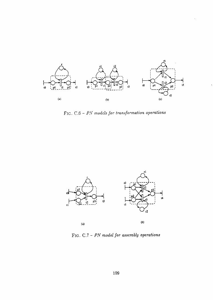
:t .:. ' -
Frc. C.7 - PN model for assembly operations
\
109

It is thus not difficult to figure out the Petri net models of the BOMs of
Pt, Pz, Ps described in Example C.1.
Example C.2
The Petri net model for the systern of Emmple C.l is shown in Figure C.8. Note
that for breuity, the processing times associated with transitions are not present.
For the saTne reason, o'nl'y the resource place r2 corresponding to rnachine M2
is present. A token in a resource place repre.sents the fact that the resource is
auailable.
,q DO tl(Ml)
|-+U+ll--
p l
17(M5)'t-+<rlO(M6)
(a) PN for Pl
"fc6-ç-5t#s--il-
e9(Ivrr)
O) PN for P2(c) PN for El
FIc. C.8 - Petri net models for P1, Pr, Pa
The following algorithm presents a general procedure for transforming BOMsinto Petri nets.
Algorithm C.l (Build Petri net model of BOMs) :----
STEP 1: Represent each buffer for semi-f,nished product as a place, called.process place. Represent each machine as a place, called resource place.
STEP 2: If atransformation operation can be carried out by m(> 1) machines,then represent the operatio'n by1 as rnany rectangle transitions (say, t1,"' ,t^) witha cornTnon input process place (toy, pt) and a cornTnon output process place (say,pz). Add crcs (p1 ,t;) antl (t ; ,pz), Vi : 1, " ' ,nr. Also arld tn other resouce places
(say, 11, - ' . , r^ ) , and ar ld arcs ( t ; , r ; ) and ( r ; , t r ) , V i = 1, " ' , rn .STEP 3: If an assembly operation can be carried out by tn(> 1) machines,
then represent the operation by as rn&nA rect'angle transitions (say, \,"',t^)with as many input process places (toA, pt," 'rp*) and one output process place
. . .f ;,1,i:::
110

(say, p*+r) . Add arc-q (p i , , t1) and ( t j ,p^+r) , V i , i - 1 , " ' ,m. Also add m other
resource Tt laces (say, 11r" ' , r^ ) , and add arcs ( t ; , r ; ) and ( r ; r t ; ) , V i :1 , " ' r f f i .
STEP /ç: Represent the procurernent operation of each raw material by a uertical
bar transition (say, \) and represent the buffer for the raw material bg a 'process
place (say, h). Add an arc (t1,py). AIso represent the di,stribution operation of
each f,nished produ,ct by a aertical bar transition (-say, t2) and represent the buffer
for the f,nished prod'uct by a process place (to'y, pr)-Add an arc (p2,t2).
STEP 5: ilIerge the process places reltresenting a comnTon buffer into one pro'
cess place representing the buffet-. tV[erge the resource place-s representing a cornnl,on
machine into one resource'place representing the machine'
C.3 Modular modelling
In the last section. rve have shoç'n horv to model lvith Petri nets a manufac-
turing system represented by the BON,Is of the proclucts it hanclles. In practice,
machines al'e gïoupecl into certain cells. some proclucts may traverse several cells
in order bo be processed on some machines in the cells it tlavetse. Therefore the
inlbrmtr[ion of machines in clifferent cel]s neecl to be taken into accottnt in the
models.Basicall;, lhere are tn'o rvavs of rnoclelling a complex manufacturing system in
a modular manner:
1. - ivlodei the modules indii'iduall-u-,
- Find the connections among the modules, and
- Compose them into the rvhole sysbem model.
2. - Inspect lhe rvhole s1'stem irom a global viervpoint,
- Cutol decompose it into connected modules accorcling to the knowledgeabout the formation of the system,
- Handle the modules and the whole system in a harmonious way.
We take the second waJ' at least for the follorving reasons:
- In the first way, once a system is a prioritreated individually, the connectionsamong the modules may be quite arbitrary and often difficult to find. Thusthis wav is of a myopic nature.
- In the second rvay, the modules ma-n. be identified from some a priori in-folmation about bhe composition of the system, moreover the connectionsamong the modules are kept cluite naturally, and the modules and the wholesystem are thus dealt with in a natural and harmonious way.
l l i

Although, in practice, how to cut or decompose the whole system into mo-dules may vary according to diferent purposes, one has to adopt certain commonpractices:
1. No two modules ale allowed to contain common machines. That is, eachmachine can only be contained in one module.
2. The size2 ol the modules should be reasonable. Two extreme cases shouldbe avoided:
- each module conta,ins only one machine,
- all machines are grouped into one module.
The former is undesilable since it does not help in dealing rvith complexityif numerous machines are present. The latter is useless since it does not takeadvantage of modulal approach.
3. Nlole often. grouping machines into cells ma.v be a complicated task if someperformance measures (e.g., rvorkload balance. inter-module traffic etc.) areto be optimized n'hile svstem topologl' sel'ves as a constraint.
lVhen machines are g-r..olrpecl into cells. the Petri net model is also broken downinbo modules. Three cases ha,r,e to be considerecl:
Case l: If m(> 2) machines performing respectively m cancatenabed transfor-mation operations (see Figr.rre C.6(b) u'hete m :2) are to be grouped intom clifferent modules, the m transitions associatecl with the m machines arefurlher separated by adding new places and transitions. This is shown inFigure C.9 where m = 2.
Ftc. C.9 - Decomposi.ng cancatenatetl transformation operati,ons
Case 2: If rz(2 2) functionally identical machines for a transformation operation(see Figure C.6(c) where nz = 2) are to be grouped into rn different modules,each transition associated rvith a machine is expanded as a subnet with an in-put transition and an output transition belonging to corresponding module.This is shown in Figure C.10 where m = 2.
2. Here the size of a module is defined to be the number of machines contained in the module.
rt2

. . : ' : , : : i l , . . ;
Frc. C.l0 - Decomposing a transformatio'n operation
Case 3: If m(2 2) tïnctionally identical machines for an assembly operation (see
Figure C.i(b) where nz :2) are to be grouped into rn different modules, each
transition associated rvith a machine is expanded as a subnet with nz input
transitions and a,n output transition belonging to corlesponding module.
This is shorvn in Fieure C.l1 n'here nt = 2.
Frc. C.11 - Decomposi 'ng an assembly operation
Consicler the s.v-stem of Example C.1. Its Petri net moclel is given in Figure
c.8.
Example C.3
Suppose that we are informed by the mt,nt,ger of the plant that the machines aregrouped into 3 cells:
- in cell 1 there are IuI1,
- in cell 2 there are tVI-o,
- in cell 3 there are NI2,
trIi, Me. fu14,
À,[a,
ùIs, l\ls, Àfrc, Mn
113

:, ;;r;;,;tr'j'idxi
Based o,n such information about cell formation, and the decomposition proce-
dure preaiously descri,bed, the Petri net models of the cells can be readily obtained
according to the d,ecom'position proced,ure preaiously described. Figure C.12 shows
the Petri net rnodel of cell 1, while the Petri net models of cells 2 and 3 are shown
in Figure C.13. The shaded places represent interface places'
FIc. C.12 - Petri net rnodel for cel l 1
C.4 System features
lVlanufacturing s5,s1sms rvith the follorving features are considered:
- Machines are grouped into cells c priori,
- Times needed to perform operations in the system are deterministic and aregiven a priori,
- The cost of holding one intermediate product and the cost for holding one
end product of all prodttct types are knon'n a priori,
- The cost of backlogging one end product is known a priori,
- No backlogging is allou'ed for intermediate products,
- Disassembly operations are not present in BOMs,
II4

'[s,TKej$-:-" ,"'d'\|-"--.yâlrE(M6) tl0(M6) i
(a) Petri net model for cell 2
(b) Pctri net model for ccll 3
Frc;. C:.13 - Petri net models for cel ls 2 and 3
Since bhe systems consiclered do not contain disassembly operations, according
to property A.11 on page 81, rve claim that the Petri net models of our systems
are CO nets.Consequently, the rvhole system can be modelled as a CO net. Each cell is also
modelled by a CO net module, the connection among the CO net modules satisfies
H6 and H7 as specified on page 72.The modular approach rve take to model such kinds of systems can be summa-
rized in Figure C.14. Basecl on the information about BOMs of the products, we
moclel the whole system l>y means of Petri net. As demonstrated previously, the
Petri net moclel is a CO net. According to the decomposition procedure presented
in the last section, the CO net model is further decomposed into interconnec-ted CO net modules. Such a decomposition is crucial to the implementation of a
hierarchical management scheme proposed hereafter.
C.5 Hierarchical management scheme
Once the Petri net moclel of the whole s}'stem is known and the decompositionof the whole system into CO net modules is done, rve propose to use a three-level
l - tpr2i
t22(M3)
115

- - ' f i ; - * r^+ i
The whole systern specified by the BOMs of the producrs
Model the systern by means of Perri ner
CO net model ofthe system
Decompose t}te CO ner model into CO net modules
C , Information needed/obtained
[-l : Decisions made
Ftc. C.11 - fu[odtilur modelling
hierat-chi cal management scheme :
- Simplified whole system planning: The goal of simplified whole system plan-
ning is to specify moclule outputs and inputs in the sub-periods.
- Cell pla,nning: Cell planning is to give procluction cluantity for each operationin each module in the elementary periods of the first sub-period. Each sub-period usually contains several elementary periods.
- Scheduling: Scheduling is to specify the start time for each firing of eachtransition in the moclules.
More precisely, the hierarchical management scheme is implemented as follows(see Figure C.15) :
1. First we simplify each module by extracting from it a minimal generatingfamily of leduced T-invariants (see annex B), which leads to a simplifiedwhole system. For example, the simplified whole system of the system pre-
sented in Example C.1 (see also Example C.2 and Example C.3) is drawn inFigure C.16. The solid black rectangles represent fictitious transitions thatlump the simplification information in terms of reduced T-invariants.
2. Based on the informabion about the simplified whole system, medium termplanning which is done on the simplified whole system can be started. Inorder to determine module inputs and outputs in the sub-periods, we take
116

. ! : - ' : i i ' . - : !1 i i ! " i r r
' - r ' . i fÈ f :3
Simplify each modulc by exracing reduced T-invariants
Simplificd wholc sysæm
Evaluatc capacity and Plan thc simplificd wholc systcn
Plan in terms of number of ætivations of each
reduced T-invtiml in tlre sub-periods
Plan cclls
Cell plans in ærms of number of activarions of ech opcrationin each ccll in thc clemcntâry pcriods of ùc first subpcriod
Schedule cells
O , Infmarion necded/obtarned
l-l , Decisions made
Frc. C.15 - Hierarchical planning
model for the simplified whole systern
Ia , i €F:'vp29
I
tII
I
LLT

as decision variables a set of scalars that correspond to the number of ac-tivations of each reduced T-invariant in the sub-periods. We then solve aminimization problem rvhich takes the sum of inventory and backloggingcosts as the objective function. This problem is subject to capacity andflow constraints. The result is the number of activations of each reduced T-invaliant in the sub-periods. From this result, it is straightforward to get theinformation about module inputs and outputs in the sub-periods (Details arepresented in section C.7).
It is rvorth noting tha,t capacity evaluation is a crucial issue for all kinds ofhierarchical approa.ches to production management (see e.g. [aa]). As such,we take a carefïl stucly of this issue befbre getting on solving the simplifiedwhole system planning problem. We plopose a simple procedure which ap-proximate 1te.:si.misticully |he s.v-stem capacity, and make use of it in planningthe simplified rvhole system.
Once the information about bhe module inpubs and outputs is given, cells canbe managecl concullently 11.1". the plemise that sufficiently large quantitiesof intermecliate proclucts are storecl in the inter-cell buffers such tha.t cellsare tlecoultled tn that ea.ch cell can function independently of the others. Inplanning each cell, u'e also sol'r'e a minimization problem which taltes theinventory costs ancl backlogging costs as objective function and is subjectto the flow and capacity constraints of the cell. Another constraint is thatthe medium term plan concerning the inputs and outpttts of the cell mustbe respected. The solution to the minimization problem is the number offirings of each transition of the module in the elementary periods of the firstsub-period. (Detai ls are presented in section C.8.)
With the results of cell planning, cell scheduling can norv be activated. Ameta-heuristic. simulated annealing, and an implicit enumeration approach,branch-and-bound, are used to deal with the scheduling task. (see also sec-t ion C.8.)
C.6 Capacity evaluation
C.6.1 Relevant notations
Let 17 be the number of sub-periocls in a planning horizon. Let H and Ë/ berespectively the length of each elementary periocl3 and the length of e_ach sub-period. Thus the number of elementary periocls in a sub-period is I{ : #.
The demand for the final product related to output transition t e Tout inelementary period k is denoled by dt,r. Thus the demand for the final product
3. We follow the convention that all elementary periods are of equal Iength
J .
4.
1 i8

;ll*:.r-i-lt!ç;,1 f;ii.,'.i-:.';'.rj;:'f;i1lri-fi$ . :
related to output transition t €Toul in each sub-period rcis: D7,^: Df;=r d4,1,.Letcrt, 0t, Vt € Tout be respectively the unit inrrentory cost and the unit backloggingcost for the final product related to output tlansition t € To,,t.
At the level of simplifiecl system planning, lve are interested in the number of
activations of the reducecl T-invariants of bhe modules. Thus it is natural for us
to take some variable associated with reduced T-invariants as decision variable.
Before doing so, let us introcluce some useful notations.Le tG j : (P juH , ,T j .F j ,À ,13 ) , i € {1 , . ' . ,N } be the j - t h Co ne t modu le , C r
be bhe incidence matrix of Gr , T!* and T!6 be respectively the set of input transi-tions and that of output transitons of Gi . Denote Tl to be the set of transitions of
Gj such that all transitions in the set are associated with the same resource repre-sented by r ( .Ri, i .e.. T! : {t € Ti l(t ,r) e Fi ancl (r, t) e Fr}. Assume that inthe simplif ied whole system there a.re totalh, ô r-educed T-invariants 21, ' ' ' , Zb.Fo reach Z i , ' i e i l . . . . . ô ) . t he remus tex i s tamoc lu l e G j , , j € { 1 , " ' . . ^ r r } o f wh i ch
Z ; i s a reduced T - inva r ian t . Le t t r r : { 1 , . . . , ô } ' + {1 , " ' . lV } be such a mapp ing ,then ir is uniquely defined by j = p,( i) € {1,. . . , /V}, Vi € {1, " ' , ô}. Let alsoT, : { i lp(i): j , l < i < ô} be the index set of recluced T-invariants of Gr.
lVe then a,ssociate n'ith each reducecl T-invariant Z; a scalat' :;,^ interpreted asthe number of activations of 21 in sub-periocl rc.
C.6.2 Evaluating system capacity
In order to plan the simplified rvhole systern, rve need to get knorvledge aboutmaterial flol ancl s1's[ern capacity.
lVhile the informabion about matelial florv is easy to get from the simplifiedwhole system model, the system capacity infolmation is not so obvious. Let Orepresent the region in which the capacity of each module Gr is not violated ifz;,"'s (Vrc,Vt € Tj) are used as the numbers of activations of the reduced T-invariants of. Gr. Since the capacity information comes from each cell, O must bedetermined via the flow of each G, and the workload of resources in Gr resultingfrom such a flow. Thus an icleal representation of O can be formulated as follows:
For each moclule Gt , j - 1.. . . , /V, for each rc, ly;, ' > 0 such that
C t x l ' i , ^=0
Yi,^[tl: t z;,^ x Z;lt], Vt e T!,U T:,t; eT t
(c.1)
(c.2)
(c.3)D v;,,,[r] x 91 1 H, Yr € HrcTl
C.1 is the f low rela[ion.
119

C.2 demonstrates that the (semi-)flowa Yi,*of z;,* for input ancl output transitions.
C.3 is the workload conclition resulting fromof transition t.
must conform to the specification
the flow Yi,*. 0t is the fir'ing time
C.6.3 An approximation of system capacity
The system capacity as defined via C.1, C.2, and C.3 represents an ideal case,i.e., the infolmation about system capacity used at the high level planning comes
from the detailed knorvledge about each module. However this does not provide
any help in reclucing complexillr, 5ince it takes a stlong flavoul of monolithicapproach.
In order to ovelcorne this difficulby, we propose the follorving algorithm to get
a simple evaluation of s-t'stem capacity in each sub-period rc.
Algorithrn C.2 (Capacity evaluation)
STEP 1: For eat'h Z;. i € T' solue the follovittg problent ahich, is to find a
flnw that minimi.ses the marintunt. worlcload of resotlrces:
subject to:
Let y; be theSTEP 2: Set
tl,[in 14/
Cr xy -0
y[t]: Z;ft l. Vt e T!,u TJ,,
LYt t l x0 , 1 l l / , Y r€HteT-
oltt imal solu,ti.on to the problem corresponding to Z;.
(c.4)
(c.5)(c.6)(c.7)
STEP S: {l ' = {(rr,.. . , zb)l D;er, z; x @;,r Ssimple pessirnistic eualuatio'n of system capacity.
if r e Hif r / H
F{ ,Vr € H, V j : 1 , . . . , / { } i s a
In STEP 1 of algorithm C.2, we intend to find out, for each reduced T-invariantZ; beloging to a moclule Gi , a flow that maximises the throughput of the module.In [128], it is shown that this is equivalent to the minimization of maximumworkload, which is the minimization problem formulated in STEP 1.
In STEP 2, we calculabe O;,, which represents the workload of resource r ifsuch a flow corresponding to Z; is followed.
4. If there is no confusion, the term "flolv" is also used. In fact, they are used interchangeablywitlr the term T-inaariant.
O,, : { Lrrrtailtlx 0"v ' ' r
I o '
120

Finally in STEP 3, we try to f ind out a set of scalars (rr," ' ,zu), where z; is
interpreted as the number of bimes we take the florv corresponding to Z;. Obviously,i f . (z;,. . . ,2a) is to be feasible, the rvorkload of each resource in each sub-period is
not allowed to exceed the length of the sub-period. Il can be proved (see Theorem
C.1) that O' is a simple pessimistic evaluation of system capacity.Note thab this approach is based. in some \r'ay, on an "ideal" production requi-
rement. But we knorv that the capacity of an agglegated system depends on theproduction mix. This nea.ns that the capacitSt computed above is an approxima-tion of the leal capacity. Furthermore, ib is impossible to evaluate how "far'" this
approximation is from the real capacity.However, we can at least prove that lhis evaluation is pessimistic, that is, using
this evaluation. it is possible to fincl a feasible solution at the next lower level. Thisis the concern of the follou'ing fheorem.
Tlreorenr C.l 0' in, STEP 3 of algori.th.m C.2 rls c pes-srrnisti.c eaalu,ation, of sys-
te'm capn,ctty.
Proof: System capacit l , ' is rept 'esentecl by' ' C.1. C.2. ancl C.3. Assume that( " r , ' ' ' , z r , ) € f ) ' , i . e . .
L t, x O;." ( 1/. Vr e -Ri. Vi = 1, " ' , /V, Vrcl e r ,
then
I ' ' I y ' [ t ] x0s1Hi€Tr teTl
or equivalently
L o,I "o x y; l t l < HrcT! ;€Tr
Set Y;,* : D;er; zi x U;, then C.3 holds.Also, since Ct * y, = 0, rve have
Cr x l'i,* --
thus C.1 holds.Finally, since C.6 holds, rve have:
tiel 1
z ; xC txy ; : 0
Yj,- l t l : t z ;xy; l t l - t z ;xZ; f t l ,ie'r r i€Tr
Thus C.2 holds. This completes the proof.
Yt e T!^u Tl,,
I2I

C.7 Simplified whole system planning
The pulpose of the sirnplified rvhole system planning is to obtain, based on the
infbrmabion about s)'stem capacity and product demands, a plan for the inputs
and outputs of the cells such that some objective function is optimised. lVe take
the sum of inventoly costs and backlogging costs as the objective function. The
goal is to minimise such an objective function over a planning horizon.In terms of Petri nets, w'e ale looking for the numbers of firings of the input
and output transitions of all the cells in the sub-periods. As explained previously,we take as decision variables the numbers r-j,6 of activations of the reduced T-
invariants in the sult-periods.The problem of planning the simplified rvhole sy'stem can be reduced to the
determination of :i.Æ's. Once the :;.^'s are knorvn fol a given sub-period n. lve then
knorv horv man.v times ea,ch teclucecl T-invariant should be activated in rc. Sincethe leduced T-invaliants concern the input and output bransitions of the modules,rve thus get a cornplebe knorvleclge about horv many times input transitions andoutput transitions of the moclules should fire in sub-period rc.
In orcler to determine :;.^'s. lve solve a rninirnization problem rvhich takes the
sum of inventorJ, ancl baclilogging costs as the objective function. and is subjectto f lorv and capacit l 'constraints.
Formalh,. the problem of calcr.tlating :;,"'s can be formulated as follows:
/\t t ;nl( I V^(./) x ̂ tq * I (o, ><,Sl^ *,Jr x S; l l
6= l q€ .Q t€Tout
subject to:
b
M^+rk) - M*(q) + I tL Zl t lx Zi .x- t Z; f t lx z; .* )i = l tQcq t eq .
(c.s)
Vq €. Q,Vrc (C.9)
(c .10)
(c.11)
b
,S , , *+r = ,5 r . * + lZ ; [ t \X z ; . * - Dr , * V teTout , v rci = l
( z ; , * , V l S i< ô ) €O ' , V rc
C.8 is the objective function rvhich has trvo items that represent different costs,The first item is the cost of token inventoly in interface places over the planning
horizon, rvhere M-(rù is the quantity of tokens (intermediate products) in interfaceplace q e Q at the beginning of period rc, and 7o is the unit inventory cost ofintermediate products in place q e Q.
The seconcl item is invenbory cost and backlogging cost of the final productsover the horizon. ̂ Sr,* is the inventory level of the buffer for the final product relatedto outpub transition t € Tout at the beginning of sub-period rc. ,SI,^ : moc{0,.91,^}is the surplus, ancl ̂ S1., - max{0,-Sr,^} is the backlog.
r22

C.9 is a constraint on the evolution of token quantities in interface places in
each sub-period.C.10 is a constraint on the evolution of quantities of final products in each
sub-period.C.11 specifies the capacity constraint that must be satisfied at the medium
term planning level. Note that the simple though pessimistic approximation O'as
proposed previously is usecl to specify lhe capacity constraint. This procedure is
i l lustrated in section C.9.
C.8 Cell planning and cell scheduling
The aim of cell planning is to obtain a plan for each cell, based on the in-
formation about cell capacib), and the simplified rvhole system plan. A plan for a
cell specifies the actua,l numbel of activations of each operation in the celi in an
elementarl' periocl.In terms of Petli nets. rvha,b is to be sought in cell planning is, for each Petri
net moclule, the number of fir'ings of tlansitions of the mocltrle in an elementary
periocl. T-invaliants ale usecl to a,cltieve this goal.The ploblem of planning rnodule Cii in the elemenlary periods of sub-period
,f can be formulated as follorvs:
tuIin t I (o' x I,;.+* + 0, x V*) (c .12)
subject to:
Yk in x 1a7t- s - ô u t
tr{t**r : I'Ii + Ci * Yo, Vk
l'i.r-+r : Vt,* * voltl - d,,u- Yt e T!,,
I Y' [ t ] x 0,1 H, Vr € ÆrrcTl
ahltl: z;,* x z;ltl, vt e T!^u Tlur, vi e TiV k i n x
The objective function C.12 reflects the fact that the sum of inventory and
backlogging costs is to be minimised. I4,r is the inventory level of the buffer for the(intermediate) product related to transition t € T!6 at the beginning of elementryperiod k.
C.13 is a token florv constraint. ù{ is the marking of module Gt in period k.yË is a T-invariant of Gj in period À'. C.14 means that a feasible flow should meet
demand recluirement.C.15 is the capacity constraint.C.16 demonstrates the fact that the medium term plan must be respected.Cell planning gives the number of firings of transitions of each cell in an ele-
mentary period. The task of cell scheduling is to determine when each firing should
(c .13)
(c.11)(c.15)
(c.16)
123

occur such that the recluirecl number of firings of transitions are satisfied in the
elementaty period.In our work, two algorithms are used to tackle this problem. One is brach
and bound (BAB) [7E], r"'hich is an implicit enumeration algorithm. The other
is simulated annealing (SA) [71], which is a meta-heuristic with analogy to the
annealing pïocess in thermodynamics. It is noted that BAB is suitable for small
problems, while for larger ones, SA should be preferred though it may, in some
cases, take a long time to get a feasible result, i.e., a schedule which enables
completion of the sholt-term planning tasks rvithin an elementary period.
C.9 Computational experience
In this section, lve repol'r oul computational experience in applying the pre-
viously proposed moclular and hierarchical approach to system management. We
first il lustrate the procedure of system capacity approximation by studying an
example, and report sorle comparative results betrveen monolithic approach and
our modular and hierarhical approach. lVe then present a complete solubion to the
management problem concet'ning the example.
C.9.1 Capacity evaluation
Consider lhe system in Example C.1. From Figure C.16, rve see that there are
6 reduced T-invariants 21.' . . ,2u (corresponding lespectively to each solid black
rectangle).Let us assume that the correspondence betlveen Z;, i e 11, i : I ,2,3 and
t eT! ,UT! , , is shorvn in Table C.1.
Reduced T-invariants Transitions concernedZ1 t:;', tza, tzsZ2 t 3s, to' t2
Z3 tsa, tnz4 ts;, t6
Z5 t l o , tsz, tgs
Za tzs, tsq
Tns. C.l - Corre.spontlence between retluced, T-ina. and transitions
then , p : {1 , ' . . , 6 } ' + {1 ,2 ,3 } i s un ique ly c le f i nec l as sho rvn i n Tab le C .2 .Thus, in this specific case, the problem of planning simplified rvhole system is
(refer to relations C.8 to C.11)
t21
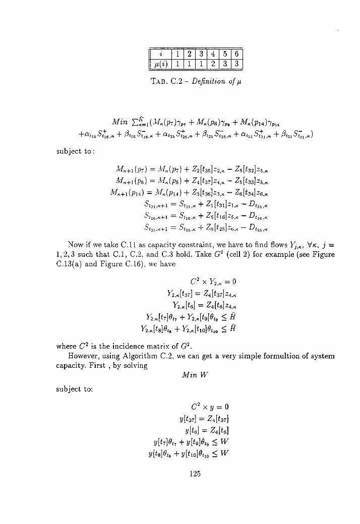
l l . : j ' i : : . r
: ; - . ia . l .
Tes. C.2 - Definition of p
Min ll)=r(M*(pr)lr, * fuI^(pù1% * fuI*(ptrn)^1o,r
1o1,u^9{u,* * l3rru.9;u," + ar."Sr+ru,* * /trrS;r,* + or' Sr1, ,n * grrr-ç;,,,)
subject to :
À,1 *+r(pr) = l{ *(p;) * Z2l45lz2,* - Z5[ts2)zs,*
h'I*+r(pr) = n./,(ps) * zalfu7]zt,^- z5lfuslz5,*ùI *+r(p,r) = ùI *(ps) + ft[fu6]4,* - Z6[fua]26,*
,5r:r,^+1 - ,5t., ,* * Zt[t"t ]rr,* - Drrr,*
-Çrre ,^+1 : -S!,.,^ t Z5lt6]25,* - Dtrc,^
5rz: , . *+r :5r r r .^ * Z6l t2s l :0 ,* - Dtzs,*
Now if we take C.11 as capacity constraint, rve have to find flows Y;.^, Vu, j -
1,2,3 such that C.1, C.2. ancl C.3 hold. Ta.ke G2 (cell 2) for example (see FigureC.13(a) and Figule C.16) , u 'e have
C2 xY l z , * -0
Y:r,*[tt l = Z.ltsi]z',*
Yz.-ltal - Zalt6lza,*,'2.^ltr]oh tY2,*ltslo1, I È
Yz*ltillî h * Y 2,*ltrclg t,o S H
where C2 is the incidence matrix of G2.However, using Algorithm C.2. rve can get a very simple formultion of system
capacity. First , by solvingMin W
subject to:
C2xy -0
ultsrl = Zn[tsrl
alt6l - Znttuly l t r )oh+yl ts lo t "<vv
ylts)|h+yltrcl î t ,o<vv
. . , . : 1 , : . ' - : . : : . ] ;-
' ; r r . r : . : : ' r : : r r : i ; : ! : i : : , i : ? : : . . ; r i
. - . . ' . . : ' : - - - . , ; - . , i i : : , 1
i I 2 3 4 a 6t"u) 1 I 1 2 3 3
r25

we get an optimal f low: tJ4: (I x t5,1 x t7, l x te, 1 x tsz), thus we have
O+,,, = va[tzlïr, + y4lts]0h : 1 x 3 + I x 4 : 7
therefore the capacity constraint corresponding to G2 is simply:
7xza lH
The above reasoning applies also to Gr and G3. IVloreover according to Theorem
C.1, we know that in doing so we get a pessimistic yet simpler approximation of
system capacity.Our computational expelience shorvs that the capacity evaluation algorithm
proposed above (Algoûthm C:.2) gives an approximation of about 4To oT the real
capacity. On the othel hancl. using Algorithm C.2 r'educes, on the avel'age, 75To of.
computabion time. This, on the rvhole, sho'ws that though Algorithm C.2 provides
a pessimistic approximation of real capacity, it is well acceptable due to the re-
duction of computation it brings about. N,Ioreover a pessimistic approximation of
system capacity gualantees the feasibility e1 the high level plan in the sense that
such a plan is implementable at the lorv level.
C.9.2 Solving a concrete example
In this section, n'e present a complete solution to the management problem of
bhe system described in Example C.1.First rve specif-v the relevant pat'ameters:
- Number of sub-periods: ,l'i = 2.
- Number of elernentary periods in a sub-periocl: Ii :2,
- Length of an elementary period: H - 50.
Table C.3 gives information about product demands.
sub-period rc = 1 st rb-per iod rc :2k : l k:2 k=3 k :4
Product 1 4 ) 4 4
Product 2 , 3 3 oProduct 3 3 4 6 3
T.q,s. C.3 - Demands inforrnation
The initial inventory information is given in Table C.4.Table C.5 presents data about inventory costs and backlogging costs.
126

Te.s. C.4 - Initial inuen,tory
Inventor)r cost, Backlogging cost
Product I l 0 50Ploduct 2 20 40Plocluct 3 30 30
Tan. C.5 - Inr;entor'y costs antl backlogging co-*ts
TAe. C.6 - Interface infor'mation
Te.s. C.7 - ,9implified whole system. Ttlanning results
Initial inventoryProduct 1 1Product 2 1Product 3 I
Initial inventory Inventory cost
Interface place P7 b D
Intelface pla.ce Pg o t0Intelface place P1.1 I 5
Cell Transition ff of firing1 tsr 61 tæ TI tso 7
I
t tsz 7
3 +r 1 6 6
3 tzs 4
127
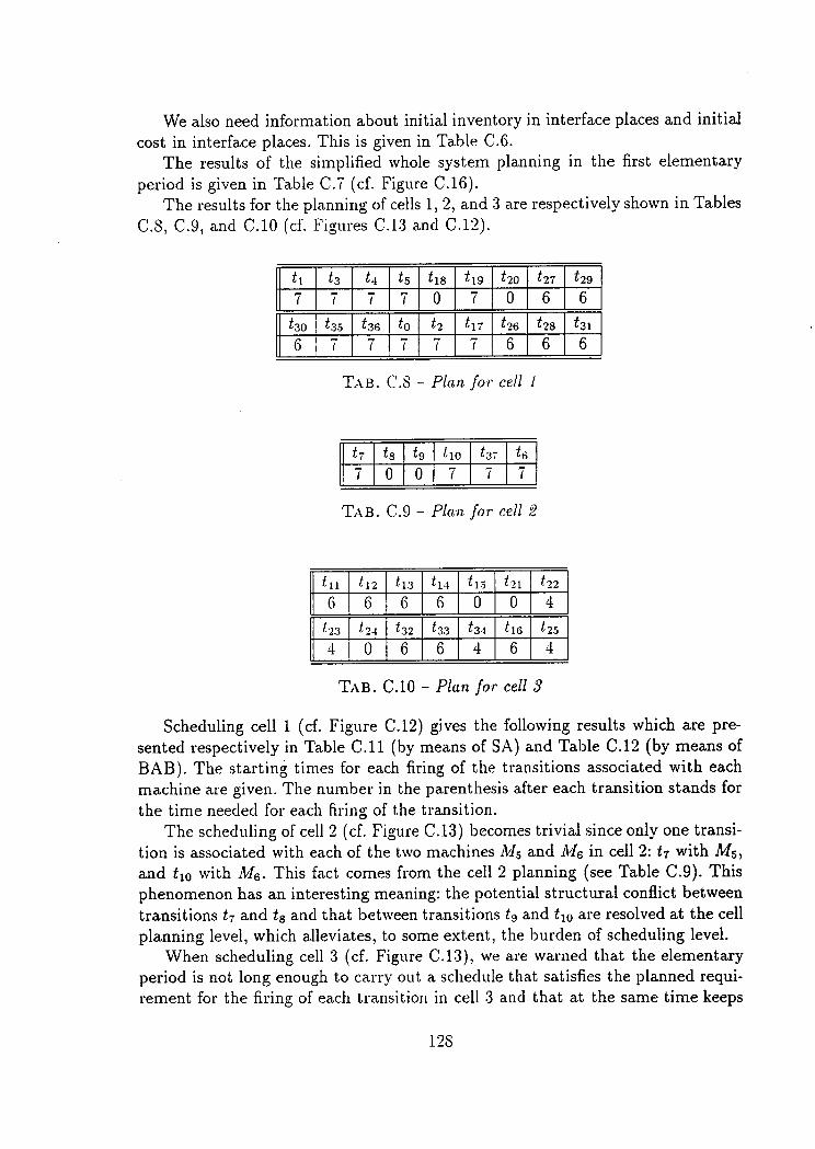
We also need information about initial inventory in interface places and initiai
cost in interface places. This is given in Table C.6.The results of the simplified rvhole system planning in the first elementary
period is given in Table C.7 (cf. Figure C.16).The results for the planning of cells 1, 2, and 3 are respectively shorvn in Tables
C.8, C.9, and C.10 (c f . F igu les C.13 and C.12) .
T.r,e. C.8 - Plan. for cell 1
Tra. C.9 - Plan for cel l 2
T,rs. C.l0 - Plan for cell I
Scheduling cell 1 (cf. Figure C.12) gives the following results which are pre-
sented respectively in Table C.11 (by means of SA) and Table C.12 (by means of
BAB). The starting times for each firing of the transitions associated with eachmachine are given. The number in bhe parenthesis after each transition stands for
the time needecl for each firing of the tlansition.The schecluling of cell 2 (cf. Figure C.13) becomes trivial since onl,v one transi-
tion is associated with each of the trvo machines .&/5 and &/6 in cell 2: t7 with Ms,and f1e with .U16. This facb comes from the cell 2 planning (see Table C.9). Thisphenomenon has an interesting meaning: the potential structural conflict betweenbransitions tz and ls and that betrveen transitions le and t1s are resolved at the cellplanning level, which alleviates, to some extent, the burden of scheduling level.
When scheduling cell 3 (cf. Figure C.i3), we ale watned that the elementaryperiod is not long enough to carry oui a schedule that satisfies the planned requi-rement for the firing of each transition in cell 3 ancl bhat at bhe same time keeps
t1 ts ta t5 l ra t rs 1120 127
I129
nI I I I U 7 0 o 6
r30 r35 feo ts t2 tt i tza It '28 +r3 l
o I I I I I b b b
! lg r9 t 1 01137
IL 6
I 0 0 7 ,7I
, l l L 1 2 t r r Ir 1 4 L l 5 , . 1 II122
o t) D o 0 0 t lT
L '23 124 132 L n 4+r3{ l ro tzs
t la 0 D 6 4 0 il
a
128

. , 1 . . - : 1 . : - : - . . : É ; : - ' - ; ! r , ; :'
l _ i ' . : i " r .5 : !
r+ ! '
the capacity of the cell within its limit. In other words, the plan for cell 3 is not
feasible. This gives us a message that we need to take some actions so that the
scheduling of cell 3 can be done. Either we must enlarge the capacity of the cell
(".g., by aclding mole machines) or we must re-start the planning by considering
a shorter planning period such that less tasks are generated for the ceils and thus
less burden is put on the cell scheduling level.
Vlachine Transition Start ing t imesfuIr f 1 ( 3 ) : 04811141821
t 2 7 ( I ) : 3 7 17 2425 26
lult t j ( 1 ) : 014561114f 1 e ( 2 ) : 19 21 23 25 27 29 31t2s(2): ' 2T912L5L i
tVIa t a (2 ) : 381315172224fso( 3 ): 51019262932
ùIt t 5 ( 5 ) : 5101520253035
Tes. C.1I - Sclt.edule for cel l I (by nteans oT SA)
N,Iachine Transition Starting times1\T, i 1 ( 3 ) : 036912L52r
t z t ( I ) : l8 19 20 24 25 26
À,1; f 3 ( 1 ) : 01258910tp(2): 361113151923t2s(2): L7 21 25 2T 29 3r
fuIe f a (2 ) : 36912151826t36( 3 ) : 20 23 28 31 34 37
ù4.t t s (5 5 10 15 2025 30 35
Tes. C.12 - Schedule for cell I (by n1'e&ns of BAB)
r29

Annexe D
Package HMPS (Hi,erarclti,cal andModular approach toPlannrng and Schedu
D.l Introduction to language Tcl/Tk
In this section. rve give a vel'y brief inirocluction to the language Tcl/Tk, andexplain wh.y rve choose Tcl/Tk tbr oul GUI development.
Tcl stands for- Tool Comrnanrl Langunge. It is a sclipting languagel and anintelpreter for that language. Tcl and its associated X rvindorv toolkit, Tk, weredesignecl and crafted b-u- John Ousterhout of IJnivelsit-v- of California Berkeley [98].
As a scripting language, Tcl is similar to other UNIX sheli languages (e.g.,Bourne Shell, C Shell, I{orn Shell etc.). But it is the ability to easily add a Tcl
l'There is no universally accepted definition of rvhat a scripting language is. However ittypically ha.s certain feabures:
- Interpreted e.xecution, so a conrpile-l ink cycle is not required.
- Simple synta.r. For example statements are usually terminated by newlines, rather than
by sernicolons or other putrctuatiort.
- Untyped variables that act as strings or numbers depending on the operations that isbeing performed ou them.
- Variables created rvhen relerenced, rather than through explicit declarations.
- High-level string nranipulation features such as concatenation, substring operations, andsearching/sorting primitives built into the language.
- No pointers or melnory allocation. Garbage collection of unused memory is done automa-ticall.v.
Another useful distinction is that scripting languages are not the same a^si macro languageswhich typically lack the control f lorv and procedure-building capabil it ies that are required in ageneral-purpose programming language.
product'ionli,ng)
130

interpreter to the application that sets it apart from other shells.There are many Tcl extensions available. Tk is one of the most notable exten-
sions. Tk has been designed for the X rvindow system, although ports to otherwindow systems are expectecl to a.ppear eventually. Tk provides a set of Tcl com-mands that create ancl manipulat e widgets. A widget is a window in a graphicaluser intelface that has a pa.rticular appeara,nce and behaviour. The term widgetand windo?o are often used interchangeably.
Although there exist several othel interactive graphical user interface develop-
ment tools, such as the Desktop Iiornshell and t\IetaCard, the reasons that we
choose Tcl/Tk for our GUI clevelopment come mainly from the following facbs:
1. Since Tcl/Tk is a script ing language,
- there is a rapicl turna,round. i.e., there is no rvaiting fbr long compila-I ions.
- the Tcl commancls provide a higher-level interface to X than most stan-dard C library toolkits.
- the graphical user interfa,ce is cleally factorecl out from the rest of theapplication.
2. The large numbel of Tcl/Tli users is a. stlong inclicatol that the use of thesetools rvill continue to inclea,se ancl their cluality rvill continue to improve.
3. The very fact ttrat Tcl/Tk is flee also makes it an attractive package fol us2.
D.2 The package HMPS
In this section, rve give an overvierv of the architecture of the prototype package
HMPS developed at project SAGEP of INRIA-Lorraine3. Emphasis is put on thegraphical user interface, i.e., human-machine interaction.
2 tclTTt is evolving quite rapidl,"-. The distributions are available by anonymous FTP from
ftp.rt.berkeley.etluin /tcl/. The.r'are a.lso available fronr harbor.ecn.purdue.eduin /pub/tcl/sprite-mirror/
3 Nlore details are reported in:
J.-ùI. Beauvil le, R.Cabirol, F. Chu, J. Grandmougin, J.-lVI. Proth, N. Sauer,L.M. Wang, SIREP - Rapport final, Spécification et Intégration à I'aidedes Réseaux de Petti des fonctions d'un système de production, Complerenilu ile fin d'opérotion d'une recherche financée par le ùlinislère d,e le Rechercheet d,e I 'Espace, Septembre, 1994.
131

D.z.L HMPS versus MASP
HIVIPS has been developed on the basis of the plototype N'IASP [115]. MASP
has three parts: human-machine interface, model definition, model evaluation.
However the structure and contents of HNIPS are different from those of IVIASP.
HX{PS has enriched all the three parts of MASP. Moreover HIVIPS has deveioped
new parts which ale indispensable to the implementation of the modular and
hierarchical managernent scheme proposed previously. Nlodel definition is enriched
to take into account the fact that the whole system is composed of interconnected
subsystems. Thus a new palt of defining subsystems (modules, or cells) is added.
Furthelmore, simplifica.tion of the modules lequires that another new part of cell
simplification be added.As fbl the evaluation of bhe system perfolmance. mole functions are added
to meet the requirements of hierarchical management. VIASP rvas implemented
under the a.ssumplion that the system is treated as an entire entity. no concept of
subsystem is involved. Since HN,IPS rvas developed under a different managementscheme, i.e.. hierarchical management of moclularl}' modelled systems, from the
one that govelnecl the implementation of NIASP, HN'IPS recptires that production
planning be carliecl out in at least ttl'o la5'e15.Thus trvo nerv palts ha.ve been built in HXfPS: the simplified rvhole system
planning and the cell planning. Nloreovel another nerv part that implements the
connection betlveen the trvo layels has also been consttucted.Finally. the graphical user interface has been re-designecl and enriched accor-
ding to the lequilements of the modular modelling and hierarchical management
fi'amervork proposecl in this thesis.
D.2.2 Architecture of HMPS
Figure D.1 exhibits the title screen of the prototype package. Please note that
all the rvidgets appearing in this section are provided by the twm window manager.If a different window manager is used, the decorations may be different.
Ftc. D.l - Title of the package
The main menu as shorvn in figure D.2 specifies the first functional hierarchyof the package. At this hierarchy, there are only two buttons that are active, i.e.,actions can be taken on these buttons rvhile nothing can be done on the buttons
HMPS
hojet SrcEPilNIÀ.tORRÀ TE
r32

lhat are not active. Thus, at this hierarchy, we can only do two things: eitherdefine a model or quit the program as shorvn in the figure.
From a user's point of vierv, the structure of the prototype consists of thefollowing steps:
- Defining a model
- Building an erecutiae product base
- Defining cells
- Specifying clemancls a,ncl getting results for- planning
- Schecluling the cells
In the rest of the section. u'e introduce these steps one ll-r' one.
Bright-font buttons: active;Dim-font buttons: inactive.
Ftc. D.2 - The rnain ntenu
D.2.3 Defining a model
Defining a moclel mea,ns that a computer recognised model of some manufactu-ring plocesses is to be built. In HNIPS. trvo wavs of defining a model are given, asshown in figure D.3: treating the input manufacturing processes as Petri nets, andtreating them as BONI (Bill of Vlaterial). Also the manutâcturing processes can
VDir modtr|n lTû$ni{rrx rle ll)tn
Colrstruinl le l*ll:t r^ûnpliti<l
IT<rnif i*; irtirll rkr lldP sirru ililbr
Flaaillimlitrr drs cs&des
[.ærcer l1]n l0ni ]?$,r:etrlent
133

, .._ .i | ,.1.
A computer recognised mo-del can be provided by ei-ther inputting with a key-board or reading from anexisting file that containsinformation of the model.
Flc. D.3 - Definitzg n model
be input rvith a keyboarcl or r.ia reacling an existing file that contains informationof the moclel.
To the best of our knorvleclge, it is a common practice to define a model with
a kel,board and by treating the manufacturing processes a.s a. BOÙI. In this case,the model is definecl bv the lollorving clua.ntities:
- number of proclttcts:
- number of machines:
- number of operabions invoh'ecl for each plocluct in the BONI;
- the characteristica of. ea,ch operation involved;
Figule D.4 gives a snapshot of hou' to inpub a model by specifying the above
mentioned cluanti ties.After the above menbionecl cluantities are input for all the products, there
remains an important thing to do: to specify the precedence constraints between
the operations. Figure D.5 shorvs how to do it in Hil,IPS. It is worth noting that
if there are more operations preceding the present operation, then the present
operation either fs an assembly operation or is not depending on the precedence
constraint given in the BOùI. For the snapshot in figure D.5, the present operation
is the one labelled 2, and there are three operations preceding it. These threepreceding operations provide semi-products asynchronousltl to the present one.The information about stoclis are to be provided.
The process of building a rnodel ends at the point that all the manufacturingprocesses are input by the lva,v just shown, and the model is saved as a file thatcontains all the information about the BOM of the products to be manufactured.Such a file will later be called a product base.
a' By characteristic of an operation, rve mean whether the operation is a simple operation
that requires only one machine, or it is a comltlex operation that requires several machines, If itrequires several machines, these machines may be used in serial or in parallel.
DEFINITION DU MODELE
lntr!.lul|€ kt models Lirs dans un flchbr
Le modele seta defmi a pMir des :
+ Reseaux de Pelri
a Garnmes de fab.ication
134
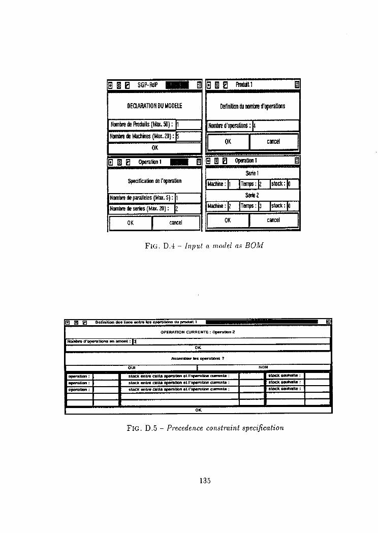
. :,-,;i:::lifÊJa'i;,,x,.*.,r1,;.*- r': : = : ' ; \ : 1 ' r " : i ' : "
DEO.ARATION DU }iODEI.[
l'lomhe ù ffiuits (l'|u. S) :
llûrtue ù hlachûnes (Mu. ?0) :
de panlleles (Mu.5) :
de sedes (Mu.2ll) :
Definilion fi nsnbrc d'opentions
Frc. D.4 - Input a motlel as BOfu[
Frc. D.5 - Precedence constraint specification
OPÊBATION CURRExTE : Op€aum Z
ilo.nông d'opeiauofts m atnoit : llOK
Bsemô&rlæo|nnt|nr ?
oul I HOll
ffit|on: slæt entE câtta opmùon gt I'oFnaùd! ffiul : ttûcl 3d.ldlt :
op.a&n: 3lrt mtrt catre opeatian ât I'ooeaÙdl G|mnla : 3læl SdtErlâ :
oF6:elbr : 3læt mlrt cetlt ofnaÙor et I'opealj.n c|mle : slOcl( 3d|ltdla :
OK
135

. , . . . : ; i , ; i l l : .._
"*i:;oij!
D.2.4 Building an executive product base
Once a product base is built, the information about all the products that can
be manufactured by a, manufacturing system in a long period of time is known.
However. in a short period of time, not all the products need to be manufactured.
Thus it is required that one choose from the product base a certain number ofproducts that ale bo be manufactured in a short period of time. This is exactly
the objective of building an executive ptoduct base.In figure D.6, it is shorvn that if a file is given in rvhich contains the information
about the manufacturing processes, then depending on the 'natures of the file, we
can choose the rvhole file to execute. or we can choose some of the processes in
the file to proceed.
Trvo possibilities: if the file itself is anexecutirre product base file. then chooseall; if the file is a product ltase file, thenchoose pa.r't of it.
Frc+. D.6 - Choosing ftn e:cecutiue prorluct ba.se from a product base file
If we choose part of the file. then we have to specify:
- horv man]- manutacluling processes ale to be chosen:
- which manttfactuling plocesses are to be chosen.
This situation is shorvn in figure D.7 in rvhich three manufacturing processes
are to be chosen, and they are the processes labelled 8,7,9.
D.2.5 Defining cells
It is up to the users to define cells. By ciefining cells, we mean the specificationof horv man,v machine groups are to be clustered, and in each machine group, howmany and which machines are to be included. These machine groups are calledcells. Figule D.8 gives a snapshot in which it is shorvn that the user decides togroups the machines into three cells, ancl in the first cell, there are four machines,they are machines 1,7,8,4.
The information about cell definition can be saved in a file, as does the infor-mation about the product base or executive product base. After cell definition isinput and saved, the main lnenu (see figure D.2) looks as shown in figure D.9.
5 Here, by "the nature of a fiIe", we mean rvhether it is a product base fi le or an executiveproduct base fi le.
Oroisir une parli€ des gammes
136

' : i trës+i.\ ' t " ',+i#RrjF ...- . i
Three processes are to bechosen, they are processeslabelled 8.7.9.
Flc. D.7 - Hou, ma?rl] and ult'ich processes to choose
Norv rve are ready to constluct a sirnplified Petri net moclel of the manufac-tuling processes in the executive product base chosen previottsly. This is done bycl ickingon the button "Constluire le RdP sirnpli f ie" (see f igule D.9). which leadsto the acti i ,at ion of the button "Planif ication cle RdP simplif ie".
D.2.6 Specifying demands and getting results for planning
Planning is concerned rvith trvo aspects: planning the simplified system, andplanning the cells. The simplified system described by a simplified Petri net isdone first. Before doing this. necessary parameters have to be specified and input.These parameters are:
- objective function: rve confine ourselves to the minimisation of the stock costsand backlogging costs. in both simplifiecl system planning and cell planning;
- number of elementary periods;
- duration of each elementary period;
- quantity of demand for each product in each elementary period;
- initial stock of each product at the beginning of first period;
- unit cost of stock of each plocluct;
Dormez b nsmrc dg chaque gatrnne
s iF Iâ gmr No. Isir la gama No. 2s t r la gamc No. 3
i 37

of CeIs(Max.1O
E El cell No.l
MaEhanes whach m:rchineM {
M 2 =H 3 =M 4 =
I
4l
There a,re 3 cells. In cell 1, thele are 4ma,chines: machines 1.7.8.4.
Ftc. D.8 - Cell definition
138

:...:.i. ild!:
Voir modele Reseaux de Petri
Ptiuifiuittj0ll r l$ ttd tt tiiiltlttith'
l:1?)r riticâtirn des c(.tll{tos
lal lc <lr I'un l$nr lix lû clrtgnl
After cell definition, morebuttons are becoming ac-t ive. cf. f isure D.2
Ftc. D.9 -:Vett ' look of main' mentL afier cel l definit ion
- unib cost of backlogging of each procluct.
For planning of the simplifiecl s1,'stem. rve a.lso need the infolmation about the
interface between the cells. This is specifiecl ll5':
- initial stock of ploclucts in the interface placesl
- unit cost of stock for ploducbs in bhe interface places.
Figure D.10 shorvs that the objective function 'die are interested in is the sum
of stocking costs and backlogging costs.Shown in figure D.l1 are rvays of inputting some other parameters. Note that
the parameter real duration of each elementary period ( not longer than the pre-
sently usecl length of periocl ) is specified in case that if the plan under the present
duration of elementary period is not feasible, we can teduce the length of period
and see if the plan under the reduced duration of period is feasible. If the present
length of period is reducecl to the real duration, and the plan is still infeasible,
then we say that rve can not find a feasible plan under the real length of elemen-
tary periocl. Othenvise we ca,n alrvays find a feasible plan under the real durationof elementary period.
lVays of inputting the interface information is shown in figure D.L2.The results of planning the simplified system and of planning cells are shown
in figure D.13. The result of planning the simplified system gives the specification
139

. r.11.
Planning data can be in-put via keyboard, or via rea-ding a file, if it exists, whichcontains the data.
Frc. D.l0 - Objecti .ue Junction
2 elementary periods;length of each period is 50;real duration of each ele-mentary period ( as a refe-rence to the presently usedduration) is 50;
Frc. D.11 - Planning parameters
t40
Oitere d'optimisafon
I Somme des cd|ts de stæl€ge et de ruplur?
O Les pretdr€ dans ur fichier
E E DtæosFulaphihtio E
ffisdcp€rioG: p
frt ôclraÇrp4ioù:150
Ilr€ æel & ch4lg p.riotb : F0
OK
Domet h rhnilde de cnqD pnrtuil i
Produit I
oæànde dM3 lr Pcriode I =omàndc dæs la psrroda 2 =S lockàto In I t i c lC$t de rlockâiaCæÈ dr rupturc
Produit 2
oamde dans la pcrlodc I =Dsrnde drns Ic pêiiodc 2 :SlockctE lnl,t l,ôlCoul dc cgockraÊCoug da ruplurc
Produtt 3
oæandê dâns la pêrlods I :oærndc dàns la pfloda 2 :SÈqckât " ln l t l c lCgut de rÈockâtèC@È d. rupcu.a
7
r0
OK

: a .:.:aa
Initial stock of product ininterface places and unitcost of ploduct in interfaceplaces are specified.
Flc. D.12 - Interface information
of the numbel of f ir ' ing t imes tbr each output transit ion of a. l l the cells during thegiven period of planning [in-re. And the outcome of planning each cell specifies the
number of firing times of every transition in the cell duling the planning period.
Frc. D.13 - Results for simplified system planning and cells planning
After the planning, only one button nLancer I'ordonnancement" is left to-be-activated in the main menu (see figure D.14). The activation of this button leadsto scheduling of the cells.
D.2.7 Scheduling the cells
Although planning a cell (as Petri net model) gives the required number offiring times of each transition in the cell so that the cost of stock and the stock
141
Donnoz las donn€€s pour l'inl4rtacÊ
ace PlFon P1ace P2loe P2acc P3Êor P3
oF ln tc rFêce p ICosÈ of stock
oÊ in t rnFàca p lCost oF suock
oF ln ts rF .cc P lCos! oF sÈock
RESULTÊTS DE LÊANIFICATION DU RESEAU SIHPLIFIE
c e I I = 135 nb-Frônch = 736 nb-Frànch = 731 nb-Frânch = 6
c . l l = 2È 37 nb-Fronc}! . - 7
c . I I = 3b 1 6 n b - F r à n c h = 6t s 2 5 n b - F r a n Ç h = 4
RESULÎAT DEFICATION DES CELLULES
c ê l l = 1E l n b - F r a ô c h = 7È 3 n b - F r â n c h = 7c 4 a b - F . r ô c t r = 7È 5 n b - F F à n c h = 7c 1 8 ^ b - F r à n c h = O
1 9 n b - F r à n c h = 7È 2 0 n b - f r à n c h = OÈ 2 7 n b - F . â n c h = 6È 29 ^b-Fràhch = €'c 3 0 ô b - F r â ô e h = 6E 3 5 n b - f r c n c h = 7c 3 6 ô b - F r â n c h = 7c O n b - F F . ^ c h = 7è 2 n b - F r . â c h = 7
1 7 n b - F r a n c h = 7C 2 6 n b - f F a n c h = 6c 2 9 n b - F r à n c h = 6

Voir modele Reseaux de Fgtti
After planning, only onebutton " Lancer I'ordon-nancerrent" is lefb to-be-activated. cf. figures D.2and D.9
FIc. D.14 - Netu look of m,ain menu' after Ttlanning
of backlogging are minimised, nothing is said about at which time the required
number of firings of each transition should occul'. This is a task to be under-taken
by the scheduling procedttles.In HNIPS, we have tahen advantage of trvo methods for the task of scheduling:
simulatecl annealing and blanch-and-bound. This is shorvn in figure D.15, in rvhich
the trvo radio buttons allolus to choose either of the trvo methods, and one can also
choose which cell to rvork on. No details are meanb to be ptesented here, interested
readers may find useful these leferences: [26] [29] [i9] [11i] [118]'
In HMPS, trvo methods areprovided for scheduling: SAand BAB.
Ftc. D.15 - Scheduling rnenu
ilûnbr ô Cêlle:3
r42

RESULTRTS E r0n!fiiillfû1tliT ff A i[iltt
l'lachine : nl ldebut de honhisarrentlt l( laps:3,00)i 0,00 3.00 6.ri0 9,û0 l2.m 15.t0 21.00i2i(tenps = t.00h 18.00 19,û0 !0.,i0 !4.00 2!.ût li.û)
liachine i m7 [debul de franhlssaent]t3(iaps:1.00): 0,00 1.00 2.00 5,00 8.00 9.110 $,C0tl9(tenrps:Z.fr): i.00 5.00 i l, ir) t i .û0 15.Ct] i9,10:3.tf)t2.e(tenps = 2.00): 1i.tt0 21,c0::.rj,l I,it 29,ic il.i{j
iiachini : n8 ldebut cie hoæirrssenent];4(larps : 2.00): i,00 É.ûr) 9.uù 12.i0 15.ù0 ir.û(t :6,Ù0ii0(iarps = i.ùù): i0.t0 2i.t0 !3.t'C il.!0 i4,i0 ii.r'I)
|tæhine : n4 ldebut de ir;rchrssanent]t5(lenps = 5,00): 5,,10 10.ù) 15,iû !i.00:5.00 ll,tt i5.tï
Scheduiing a cell gives thestarting instant of each fi-ring of the recluirecl numberof firings for each transitionin the cell .
Frc;. D.1[i - Scheduling result
D.3 Conclusion
A prototype package H\,IPS is presented. It is clesignecl on the basis of modularmodelling ancl hieralchical ma,na.gemenb of manufacturing systems. The moclular
modelling rvork is clone in the frameu'ork of Petri nel bheory. We ploposed a
new type of Petli net, CIO net. t,o specificalll' tailol the recluirement of modular
moclelling a.nd system intr-:gration. lVe also proposed an efficient algorithm for
simplifying a given Petri net moclel in the sense that the net structure is simplifiedrvhile the input-oubput flou' r'elation of the original Petri net is preserved. The
a.lgorithm applies not only to CO nets but also to general Petri nets. The use
of the package is fa,cilitated b.v a graphical user interface designed in languageTcl/Tk.
Although the preliminar.r' use of the prototype pa.ckage shows that it is ca-
pable of solving sorne problems quite satisfactorilv, ihere still remains a longrvay to go to get it cornpebitive rvith existing commercial packages, like PRO-VISA (AT&T), WITNESS (AT&T), AutoSched (AutoSimulations), QUEST (De-
neb Robofics Inc.). N,IPX (Netrvorl i D1'namics Inc.), FACTOR (Pritsker Corp.).IvIanSim/X (TYECIN Systems Inc.). to name a few.
Some perspectives we envisage are as follorvs:
- There is room to the improvement of the graphical user interface. As seen
l+3

from the previons introduction to HNIPS, the rvhole GUI is principally ba-
sed on a button actiaation scheme, lvhich has been shown to be clumsy.New versions of Tcl/Tk have provided enhancement on pull-clown menus,which enables procluction of more friencll,v, more agreeable huma.n-machineinterface.
Plesent rvays of inptrt,t,ing product base lack flexibilit"v and robustness. New
options. like stochastic processing times ancl nelv BON'{ stluctures. are cliffi-cult to get incorpora.t,ecl into fhe present package beca.rtse of the rigicl struc-tule of the paclta.ge. \lole fault-tolelant mechanisms neecl to be incorporatedso that er-ror- messa,ges not only are elror inclicators but also ale inforrnativein fincling out rvhele bhe elrors are. To sum up bliefly, a cribical r:e-design
from the point of vieu'of sottrva.r'e engineering needs to be examined.
As tbr the methocl o[ pla.nning aclopted in I-I\'IPS. natnel.r' an open-looplop-clorvn planr-r ing pra,ct ice. plan l 'easibi l i t l ' pLoblem is a plominent issue.
Although therr,: a,re some c[iscussions about this issLre in the l i terature. seee.g. . [36] , [76] , [3 ] ] [3 l t ] . a s i rn l>[ec losecl - loop pract ice c loes not const i tu te thee1111' 11,n.1, out. t ,heoretir:al l-r. sorrncl ancl practical l l ' eff icient a.pproaches are
alrva,r.s in urgent ner:cl.
Though schecltrling problems are generally cluite notot'iotts [i1] [32] [a1]. andsimulatecl annealing a,ncl branch-ancl-bound methods are tlvo frecluently usedmethocls to deal rvit,h them, nen' a.tta,cks a,l'e altt'art's a.ttemptecl as ca,n be seentltrough the enormous art icles on [his issue. It might be f luit ful to incorpo-rate variorrs a.pptoâ,ches to I-lI,lPS a,ucl acla,pt thern to clifferent practical
situa.t ions.
.\s pointecl out, previorrslr ' . a nes' look at the package FIN{PS from the soft-n'are engineering point, o[ r'ierv is certa.inll' necessary if the aim of HIvIPS is to
be competitive rvith existing comlnercial pa.ckages. Various tricks in dealingwith the efficient use of memol'y spa.ce and reducing time consumption are'horvever, also inclispensable to get iI compact enough to solve larger practicalproblems.
l4-l

Bibliographie
K. Aarclal a.nd T. Larsson. A benders decomposition based heuristic for the
hierarclrical production planning problem. Euroltean Journal of Operational
Research. 45:-t-14. 1990.
T. Agelwala ancl Y. Clhoed-Arnphai. A synlfi"t1t rule for concurlent s.ystems.
In Proc. lSth De-ci,gn. Autontation Confergnce, pages 305-331, Las V'egas.
June 1978.
R..Y. Al-Jaar a,ncl A..\. Desrochels. Petri nets iu automation and manu-
tâcturing. In "ltluutcr',s rln ,{ utontu.t.i.otr. nnrl Roboti.c.s. volume 2. JAI Press,
1989.
R.N. Anthony. Planni,ng and control sy.stems: a ft'arnework for analysis. Har'varcl Llniversity Pr-ess. Ciraduate School of Business Aclministration, Cam-
briclge, lVlassachussettes, 1965.
Ch. Ausfelder', E. Castela.in, and J.-C. C'lenlina.. A method for hierarchicalmoclelling of the command of flexilile manufa,ctuling s,v-stems. IEEE Trans.
Systems, ùIan and Ctlbernetics, 2.1(1):564-573, 1994.
S. Axsater. On the design of the aggregate model in a hierarchical production
planning system. En.gineering and Process Economics, 4:89-97, 1979.
[7] S. Axsater. Aggregation of product clata tbr hierarchical production plan-
ning. Operations Research, 29$):7+a-756, 19E1.
S. Axsater. On the feasibility of aggregate procluction plans. OperationsResearch, 2a$):7 96-800, 1986.
S. Axsater and H. Jonson. Aggregation ancl clisaggregatiuon in hierarchicalprocluction pla.nning. Euroltean Jou.rn,al. of Operat,ional Research, 17:338-350, 1984.
S. Axsater, H. Jonsson, and A. Thorstenson. Approximate aggregation ofprodnct data. En,gineeri.ng Cost anrl Protluction Economics, 7:119-126, 1983.
t1l
l'rlt - l
t3l
t4l
r p l
tol
t6l
t8l
tel
[10]
145

[11] I{.R. Baker. Int'rorl'uctiort, to sequencing and -ccheduling. Wiley, New York,
1974.
[12] J. Benassy. La gestion de productàon. Hermes, 1987.
[13] A. Bensoussan, lVI. Crouch;" and J.IVI. Proth. Ù[athematical Theory of Pro-
duction Planning. Elsevier Science Publishers 8.V., 1983.
[14] G. Berthlot. Checking properties of nets using transformation. In G. Ro-
zenberg, eclitor', Ad'uances in Petri Net.s 1985. Lecture Nobes in Computer
Science, pages 19-,,t0. Springer-Verlag, 19S5.
[15] G.N,I. Biltu'istle. DEl,lOS: A system for disuete euent rnodelling on SI-
I,I U L A. .t\IacùIillan. 1979.
[16] G.R. Bitran, E.A. Haas, and A.C. Hax. Hierarchical ptoduction planning:
a single stage system. Oqterations Research,29(a):717-743, 1981.
[17] G.R. Bitran. E.A. I-Iaas. ancl A.C. Hax. Hierarchical production planning:
a, t'r,r'o stage s-r,'sten't. Opr:rntions rr:se;ctt'ch. :10(2):232-251. 1982.
[1S] Ci.R. Bitran. E..\. I-Iass. ancl I{. \ , [atsuo. Plocluction planning of st,"- le goods
rvitlr setnp costs ancl forecast revisions. Operati.ons Re.search,32(2):226-236,1986.
[19] G.R. Bitran ancl A.C. Hax. On the clesign of hierarchical production plan-
ning systems. Deci.si.on, Sciences, 8:28-55, 1977.
[20] G.R. Bitran .nd [.fI. Hax. Disaggregation and resoutce allocation using
convex knapsack problems lvith bounded variables. l[anagement Science,
27Q):a3l -44 i , 1981.
[21] G.R. Bitran and D. Tirupati. Hierarchical production planning. Technical
Repolt 3017-89-ivIS. N'IIT, Sioan School of Nlanagement, Cambridge, 1989.
[22] IvI.R. Bowers and J.P. Jarvis. A hierarchical production planning and sche-
duling model. Decision Sciences, 23(1):1aa-159, 1992.
G.'vV. Brams. Reseuux de Petri: Theorie et Pratique. MASSON, 1983.
J.A. Buzacott ancl J.G. Shanthikumar. Design of manufacturing systemstrsing qtreueing moclels. Qu,ettei.ng Systerns, 12:135-214, 1992.
J.A. Buzacott a.nd J.G. Shanthikumar. Stochastic models of manufacturingsystems. Prentice-Hall, Englewood Clifs, NJ, 1992.
[23]
[24]
[25]
1,16

[26]
l27l
[28]
IrolL . ! J
[30]
[31]
[32]
[33]
J. Carlier and P. Chretienne. Timed petri net schedules. In G. Rozenberg,editor, Aduances ùt Petri nefs, volume 340 of. Lecture Notes in ComputerScience, pages 62-84. Springer-V'erlag, 1988.
C. G. Cassandras and P. J. Ramadge. Toward a control theory for discreteevent systems. IEEE Control Syste'ms A'Iaganizine, pages 66-111, June 1990.
C.B. Chu, F. Chu. J.-M. Proth, and X.L. Xie. Veli f ication incrementale
de la consistance d'un Leseaux de petli. to appear in Technique et ScienceInformatique, 1995.
F. Cjhu. J. N,I. Proth. ancl V.N{. Savi. Ordonnancement basé sur les réseauxde petri . Technical R.epolt 1960, INRIA, 1993.
G. Cohen, D. Dttbois. J.P. Quadrat, and NI. Viot. A l inear system theore-tic vierv of discrete event processes ancl its use for performance evaluationin nranufactuling. IEEE Tran.s. Automatic Control. 30(3):210-220, Nlarchr985.
G. Cohen, P. N'Ioller. .1.P. Quadt'at. a.nc[ N'I. \ôit. Algebraic tools for theperlbrmance evalnation of disclete et'ent systems. In Proceedings of the
IEEE [61]. pages 39-58.
R.\,V. Conway, !V-.L. Nlaxrvell. and L.W. Nliller. Theory of scheduling. Ad-dison !Vesle5', Nlassachussetts, 1967.
R.A. Ctrninghame-Green. tr[ininnr Algebtz, volume 166 of Lecture Notes inEconomic and l,[nthetnotical Systems. Springer-Verlag. 1979.
S. Dauzere-Peles. Planifcation et ordonnance'ment de Ia production: uneap'proche integree coherente. PhD thesis, Universite Paul Sabastier de Tou-louse, March 1992.
R. David ancl H. Alla. Du grafcet atrt résea'ut de Petri. Edition Hermès, 2eédit ion, Paris, 1992.
[36] IvI.A.H. Dempster' , M.L. Fisher, B.J. Lagweg, L. Jansen, J.K. Lenstra, andA.H.G. Rinnooy I(an. Analytical evaluation fo hierarchical planning sys-tems. Operations Research, 29(a):707-716, 1981.
[37] F. DiCesare, G. Harhalakis, J.NI. Proth, IVI. Silva, and F. Vernadat. Practiceof Petri nets in manufactttring. Chapman and Hall, 1993.
[38] S.E. Elmaghraby. The economic lot scheduling problem: review and exten-sion. ùIanagement Science,, 2a(6):587-598. February 1978.
[34]
[35]
r17

[39] J. Erscheler, G. Fontan, and C. Nlerce. Consisbency of the disaggregationprocess in hierarchical planning. Operations Research,S4(3):464-469, 1986.
[40] C.A. Fernandes and F.A.C. Gomide. A heuristic procedure for productionplanning of modern manufacturing systems. Corn'puters and Industrial En'gineering, 20$):a7 5-485, 1991.
[41] S. French. Sequencing and scheduling. John Wiley and Sons, 1982.
[42] L.F. Gelders ancl L.N. van Wassenhove. Production planning: a review.European Jou,rnal. of Operational Reseat'ch, 7:I0L-I10, 1981.
[43] L.F. Gelders ancl L.N. r,an lVa.ssenhove. Hielarchical integration in pro-
dtrction planning: theor-v- ancl plactice. Jow-nal of Operations il[anagement,3 (1 ) :27 -35 , 1982 .
[44] S.B. Gershrvin. Hiera.rchical florv control: a framervork for scheduling andplanning disclete events in manufactuling s-v-stems. In IEEE Proceedings,Special Issue on rES. [61].
[+i] V. Cliarcl. CJe.stion de lu producti.on. Economica. 2ncl ecl i t ion. 19EE.
[46] P. Gla,sserma,n ancl D.D. Yao. Cieneralizecl semi-malkov pt'ocesses: anti-matroicl stmctule ancl second-oldel properties. A,Iathematics of OperationsResea,rclr, 17(2):aa4-469, May 1992.
[4i] P.\,V. Glynn. A gsmp formalism for discrete event systems. In Proceed,ingsof IEEE [61], pages 1.1-23.
[48] XrI. Gondran ancl iV[. ]Vlinoux. Graphes et algoùthmes. Eylolles, Paris, 1979.
[49] G. Gordon. The application of GPSS lr tu discrete system simulation.Prentice-Hall, Englervood Cliffs, NJ, 1975.
[50] S.C. Graves. Unsing langrangean techniques to solve hierarchical productionplanning problems. ùlanagement Science.s, 28(3), 1982.
[51] H.ivI. Hanisch. Analysis of timed petri nets by means of dynamic graphs.Petri Net Newsletter, 36:24-31, 1990.
[52] H.M. Hanisch. Analysis of timecl place/transition nets using minimal stategraphs. In G. Cohen and J.P. Quadrat, editors, (Ith International Confe-rence on Analysis anrl Oltti.misation of Syste'rns, r,olume 199 of Lecture Notesin Control and InJorm,ation Science.c, pages 205-212. Springer-Verlag, June1994.
148

[53] G. Hathalakis and J.NI. Proih. Some open problems in the design and use ol
nrocleln producbion svsterns. Apytlied Stochastic N[odels and Data Analysis,
7 :33 -45 ,1991 .
G. Harhalakis, J.lvI. Proth, and X.L. Xie. A comprehensive approach of
planning and schecluling based on petli nets. Applied Stochastic Models and
Data Analysis, 9(3):1S7-213, 1993.
C.J. Harris. Out of control into systems engineering research. In 1lth Com-
puting and Control Lecture, Savoy Place, London, Feblualy 1994. IEE'
I. Hatano, I(. Yamagata,, and H. Ta.mura. ÙIodelling and on-line scheduling
of flexible manufactuling sy5lsrns using stochastic petri nets. IEEE Trans.
Software Engin eering. L7 (2):L26-132, Febrttary 1991.
A. C. Hax and H.C. Nleal. Hierarchical integration of production planning
ancl scheduling. In I'I.A. Geisler, editor, Stu,tlies in ÙIanagement Sciences,
volume I, pages 53-69. North Holland - American Elsevier'. 1975.
.J.!V. Hermanr. r\ . \ , lel i la. I . \ , l inis. ancl .J.N,I. Proth. Fl ieralchical production
planning ',r,ith palt, spa.tial ancl time agglega.tion. In Proc. ,lth Int. Conf.
on clful and Autotnr,tion Technology, pages 430-435, Reselaer, New York,
Octobel l994.
H. P. Hillion and J. N'1. Ploth. Perfot'mance evaluation of job-shop systems
using t imeclevent-glaplts. IEEE Truns. Au,tom.atic Control,34(1):3-9' 1989.
Ivl.H. Hillion. tr[otlelisat:ion et analyse des systemes de 'procluctoin discrets
par les reseauî. rle Pet.ri. ternporises. PhD thesis. Universite Pierre et Marie
Curie, Paris VI, Januar,u- 1989.
Y.C. Ho, editor. Special iss.ue on dyntnùcs of discerete euent systems, vo-
lume 77 of. IEEE Proceedings, 1989.
[62] Y.C. Ho and X.R. Cao. Pertu,abation analysis of discrete euent dynarnic
systerns. Klurver Academic Publishers, 1991.
[63] C.A.R. Hoare. Communicating Sequential Proce.sses. International Series in
Computer Science. Prentice-Hall, 1985.
[64] B.W. Hollocs. Imploving manufacturing operations with witness computer
s imulat ion. ATUT Technology, 6(1) :16-21, 1991.
[65] L. E. Holloway and B. H. Iirogh. Synthesis of feedback control logic for a
class of controlled petri nets. IEEE Trans. Autornatic Control,,35(5):51a-523, 1990.
[54]
lool
[56]
|.D rl
[58]
[5e]
[60]
[61]
149

[66]
[67]
[68]
[74]
I roJ
li6l
[6e]
[70]
I J I I
l i2l
li3l
K. Inan and P. Varaiya. Finitely recursive process models for discrete event
systems. IEEE Trans. on Automatic Control, 33(7):626-639, July 1988.
R.R. Inman and P.C. Jones. Decomposition for scheduling flexible manu-
facttrr ing systems. Operations Research, l(3):608-617' 1993.
K. Jensen. Coloured Petri nets: Basic concepts, analysis rnethods and Ttrac-tical use, Vol.1. EATCS t\Ionographs on Theoretical Computer Science.
Springer-Verlag, 1992.
U.S. Karmarkal ancl L. Schrage. The deter-ministic dynamic product cy-
cl ingproblem. Operation,s Researcl2, 33(2), 1985.
J. Iiimemia. ancl S. B. Clershrvin. An algorithm for the computer control of
a. f lexible ma,nufactr.rr- ing system. IIE Transations, i5(a):353-362, 1983.
S. Kirkpatr.ick, C.D. Gelatt, and t\,I.P. \'ecchi. Optimization by simulated
annealing. Science. 220(a598):671-680, NIa."- 1983.
I. I(oh and F. DiCesale. Nlodular transformation methods using deviation
botrnds in automatecl ma.nufacturing s.v-stems. IEEE Trans. Systems, It[an
and Cybernetics. 21(6):1512-1522, 1991'
A. B Ktrrzlranslçi and P. Vâraiya, editors. Discrete euent systems: ùIodels and
aytplications. volume 106 of Lectut'e Notes on Informution Sciences. 1988.
S. Laftit, J.N,I. Proth. ancl X.L. Xie. Optimisation of invariant criteria for
event graphs. IEEE Tr7ns. on Automatic Control,:17(5):547-555, 1992.
L.S. Lasdon and R.c. Terjung. An efficient algorithm for multi-item schedu-
ling. Operations Research, 19, I97I.
J.B. Lasserre. An integrated model for job-shop planning and scheduling.
Management Science, 38(8):1201-1211, August 1992-
[i7] J.B. Lasserle, J.P. Nlartin, and F. Roubellat. Aggregate model and decom-
position method for mid-term production planning. International Journale
of Production Researcâ, 21(6):835-843, 1983.
[78] E.L. Lawler, J.I{. Lenstra, A.H.G. Rinnoy l{an, and D.B. Shimoys. Se-quencing and scheduling: algorithms and complexity. Technical Report NFI
11.89/03, Eindohoven University of Technology, November 1989.
[79] D.Y. Lee and F. DiCesare. Fms scheduling using petri nets and heuristic
search. In Proc. 1992 IEEE Int. Conf. on Robotics and Automation. pages
1057-1062, Nice, France, \ ' Ia1' 1992.
150

[80] I{.H. Lee and J. Favrel. Hierarchical leduction method for analysis anddecornposition of petri nets. IEEE Trans. Ssystems. ÙIan, nnd Cybernetics,15(2) :272-281, 1985.
K.H. Lee, J. Favrel, and P. Baptiste. Generalized petri net reduction method.IEEE Trans. on Sy-stenrs, X{arz, ancl Cybernetics, 17(2):297-303' 1987.
G.K. Leong, NI.D. Oliff, ancl R.E. i\'Iarklancl. Improvecl hierarchical produc-
tion planning. J ount al of O perations fuIanageme'nt, 8(2) :90-1 14, 1989.
C. Libosvar. Hi,erarchical producti.on ïLanagernent: the fl,ow-control layer.PhD bhesis, Université cle Nletz, 1988.
C.W. Lin and Ci.L. N{oodie. Hiela.rchical ploduction planning for a modernsteel rnanufacturing srrstenl. Internati.onal Jonrnal of Production Research,27 (a ) :613 -627 , 1989 .
J.G. Long. Su'lu, con.duite hierarchisee des .systemes fleribles de p'roduction.PhD thesis, L'Instibut National Polytechniclue cle C'h'enoll le, June 1993.
A.G.J. NlacFallane. Inlbrmation, ltnowleclge ancl control. In H.L. Trentelmanand J.C. Willems, eclitors. Essuys on Con.trol: Per.spectit-,es in the Theoryan.d its Applicution-s, t'olnme 14 oT Progress in Slystems and Control Theory,pages 1-28. BiLkhâuser Boston, 1993.
lvl.S. Nladan and I{.C. Gilbert. An exa.ct solution algorithm for a classfo procluction planning and schecluling proltlems. Operations Research,a3(10) :961-970, 1992.
J. Nla.rtinez ancl NI. Sih'a. A simple and fast algorithrn to obtain all invariantsof a generalisecl petri net. In ?nd European Worleshop on Application andTheory of Petri n efs, pages 411-422, 1981.
[S9] A. lvlehra. Design u'nd unal'ysis of hierarchical production planning systems
for 'purallel com'putittg enait'onments. PhD thesis, University of Maryland,1995.
I{. Ivleier. Commanrle hiérarchisée d'un sl1stème tle production. PhD thesis,Université de Metz, January 1989.
J.G. rVliller and A.V. Roth. A taxonomy of manufacur:ing strategies. Iv[ana-gement Science, a0(3):285-304, ivlarch 1994.
[92] T. tVltrrata. Petri nets: properties. analysis a.nd applications. Proceedings ofI E E E. 77 (a):5aF580, 1989.
[81]
[82]
[83]
[8-r]
[85]
[86]
[87]
Is8]
Ie0]
[e 1]
151

[93] R. Nagi. Design and operation of h,ierarchical production rnanagement sgs-
tem.s. PhD thesis, University of Maryland, 1992-
[94] S.J. Nam and R. Logendran. Aggregate production planning - a survey
of moclels and methoclologies. Euroytean journal of Operational Research,
6I:255-272, 1992.
[95] Y. Narahari and N. Viswanadham. A petri net approach to the model-
ling and analysi5 of flixible manufacturing s1'stems. Annals of Operations
Research, pages 449-'t72, 1985.
[96] J.J. O'Reilly and N.Ii. R)'on. Intloduction to slam ii and slamsystem. In
Proc. of 1992 l4ti.nter Sinu,lation Conference, pages 352-358, Arlington, VA,
USA, Decernber 1992.
[9i] J.S. Ostroff a.ncl \\I.\1. \\/oham. A frame*'ork fol real time discrete event
control. |EEE Trntls. on ; luton.atic C'ontrol. 35(a):386-387, Apri l 1990.
[98] J. OusterhouL. Tcl nttrl the Tk toolkit..\clclison-\Vesle;' Publishing Company
Inc. . 199-1.
[99] C.D. Petden. R.E. Shannon. a,ncl R.P. Saclos'sl i i . lnirodttct ion to simulation
with, SIùlArY ùIcGra.rv-C'lill. NJ, 1990.
[100] J.L. Peterson. Petri. nc:t theory and the morleling of .s!J-qte'rn.s. Prentice Hall,
Inc., Englervoocl Cli f fs, N.J.. 1981.
[101] J.I, I . Proth ancl I . ù{inis. Plocluction management in a petri net environment.
Reclt erche o 1t é rut i , o nn e I I e. '29 (.3) :32 I -352, I 995.
[102] J.N{. Proth, N. Sauer, Y. Wardi, and X.L. Xie. Nlarking optimisation of
stoclrastic timed event graphs using ipa. In 32nd IEEE Conf. on Decision
ancl Control, pages 686-691, San Antonio, Texas, December 1993.
[103] J.À{. Proth, N. Sauer. and X.L. Xie. Stochastic timecl event graphs: bounds,
cycle time reachabilit,.,- and marking oplimisation. Technical Report 1763,
INRIA, France, 1992.
[104] J.N4. Proth and X.L. Xie. C1,'cle time of stochastic event graphs: evaluation
and marki ng optimisa.t ion. I E E E Trans. on A'uto mnatic C ontrol, 39(7) : 1482-1486, July 1994.
[105] J.NI. Proth and X.L. Xie. ,Les reseaur tle Petri pour Ia conception des sys-tem,es de prorhtct ion. IVIASSON, 1995.
[106] P. J. Ramadge and \,V. N{. lVoham. The supervisory control of a class ofdiscrete evenb s.v-stems. SIAITI J. Control rtnrJ Optimi:ution,25(1):206-230,Janualy 1987.
r52

[107] P. J. Ramadge and \,V. X{. lVoham. The control of discrete event systems.In Proceedings of IEEE [61], pages 81-98.
[108] C. Rarnchandani. Ana,l.vsis of asynchlonons conculrent systems using petri
nets. Technical Repolt 120. MIT, Cambticlge, MA, 1974.
[109] \,V. Reisig. Petri net.s. An Introductàon, volume 1of. EATCS lVlonographs onTheoretical Co'mputer Science. Springer-!erlag, 1985.
[110] NiI. Rose. Plodr,rction planning at texas instmments improves service andreduce costs. Industriul Engin eering, 23(1):33-36, 1991.
[111] \,V.G.iU.iVI. Rutten. Flierarchical mathematical programming fo roperationalplanning in a, process inclustrl'. European JourncLl of O'perational Research,64:363-369, 1993.
[112] G.H. Saad. Hierarchica.l plocluction planning syslsl ls: extensions and mo-cl i f ications . Operution.s ResearcÀ. 41(7):609-621. I990.
[113] 1\,I. Sajkorvski. Plotocol verification using cliscrete et;ent models. In Iiurz-hanslii and Varai]'a [73], pages 100-114.
[114] N. Sauer. Les graphes cl 'euenements stochastiques et leur uti l isation pourl'euriluation des s11stem,e.s de prorlucti.on. PhD thesis. Universite de ivletz,September 1994.
[tt5] \i. Savi. Conception préliminaire rle.s système.s de produ,ction à l'aide desréseatrr de Petri: éunlttati.on des lterforùt,trnces. PhD thesis, Univetsité deN le tz ,1994 .
[116] V.i!I. Savi and X.L. Xie. Liveness and boundedness analysis for petri netswith event graphs rlodules. In I( Jensen, editor, Application and Theoryof Petri Nets 1992, Lecture Notes in Computer Science, pages 328-347.Springer-Verlag, 1 992.
[117] L. Shen, Q. Chen, and J.Y. Luh. Truncation of petri net models for simpli-fying computation of optimum scheduling problems. Co'mputersin Industry,20(L):25-43, 1992.
[118] H.lvI. Shih and T. Sekiguchi. A timed petri net and beam search based on-line fms scheduling system with routing flexibility.ln Proc. 1991 IEEE Int.Conf. on Robotics and Automation, pages 2548-2553, Sacramento, Califor-n ia , Apr i l 1991.
[i19] J. Sitâkis. Use of petri nets for performance evaluabion. Acta Cybernet,a (2 ) :185 -202 ,197E.
153

[120] ivl. Silva and R. Valette. Petri nets and flexible manufactudng. In G. Ro-zenberg, editor', Aduances in Petri nets, volume 424 of Lecture Notes in
Computer Science, pages 374-416. Springer-Verlag, 1989.
[121] P.H. Stark. Arc timecl net analyser. Petri Net Neusletter, 37:27-33, 1990.
[122] I. Suzrrki and T. lVlurata. A method fol stepwise refinement and abstractionof petri neîs. Jour'nal of Computer antl Systems Sciences, 27:51-76, 1983.
[123] S.D. Thompson ancl !V.J. Davis. An integrated apploach for modellingtrncertainty in aggregate production planning. IEEE Transactions on SI[C,20 (5 ) :1000-1012 . 1990 .
[124] S.D. Thompson, D.T. \\atanabe. and !V.J. Davis. A comparative studyof aggregate production planning strategies under conditions of uncertaintyancl cyclic proclnct clemancls. International Jorn'nal of Produ,ction Research,31 (8 ) :1957-1979 , 1993 .
[125] H. Tsr,rl>one. FI. tr,latsura.. and T. Tsutsu. Hieralchical production plan-ning s-v-stem fbr a, tu'o-stage process. Interncûionnl Jourtzal of Protlu,ctionReseut-ch^ 29(+) :769-785. 1991.
[126] R. \,'alette. AnalS'sis of petr-i nets by steprvise refinements. Journal of Com-puter ans System Sciences,18:35-46, 1979.
[127] L.N. lVassenhove and L.F. Gelclels. Hierarchical integration in productionplanning: theory and practi ce. Jou,rnal of Operations Ùlunagement, 3(l):27-35, 1982.
[128] X.L. Xie. Controle hiexrrchique d'un lystente tle ytroclu,ction sou,rnis & per-turbati.ons. PhD thesis, Universite de Nancy. June 1989.
[i29] X.L Xie. Supelposition properties and performance bounds of stochastictimed event graphs. IEEE Trans. on Autornatic Control, 39(7):1376-1386,July 1994.
[130] X.L. Xie. Analyse, concepûion et contrôle des systemes de production. Habi-litation à diriger des lecherches en sciences, Univeristé de Metz, IVIay 1995.
[131] G. Zapf.el and H. t\lissbauer. Nerv concepts for production planning andcontrol. Euro1tean J ournol of Operational Research, 67 (3):297-320, 1993.
[132] lvl. C. Zhou, F. DiCjesare, and A.A. Descrocher. A hybrid methodologyfor synthesis of petri net models for manufacturing systems. IEEE Trans.Robotics and Au,tomation, 8(3):350-361, 1992.
' i jrr lÉ+::i i :
154
I

[133] VI. C. Zho,,t, F. DiCesare, and D. L. Rudolph. Design and implementation of
a petri net basecl moclels for manufacturing system. Automatica,23(6):1199-
1208, 1992.
[134] P.H. Zipkin. Compubing optimal lot sizes in the economic lot esheduling
problem. OTterations Research, 39:56-63' 1991'
[l3b] K. ZoIler. Optinal disa.ggregation of aggregate production plans. fu[anage-
ment Sc ience, l7(8) :533-579, 1971'
t55

Index
SymbolesNR
Aaccessible
acyclic system
aggregat ion . . . .
arbre de r-ecouvrementarbre des marquages atteignables
a s v n c h r o n e . . . .
BBON{ . . 133
cco . . . . . . . 3s,
consistentidentification ofIive .reversibleunbounded
Confliteffectifstructurel
consis tency . . . .contracted graphcut and simplify
Dd iv ic le and conquer . . . . . . . 95
FFMS 1franchie
une séquence de transitious 11
12S6
11l a
8815152
Ggenelat ing fami ly . . . . . 43, 87graphe d'événements . . . . . . 12GUL . . 132
Ii rnp l i c i tp lace . . . . . . .70in te r face t ra ,ns i t ion . . . . . . . . 88
Lla5,s1 .
I iveness
Mméthodes de synthèse .. . .
méthodes ascendanteméthodes descendantes . . . . . .
méthodes de transformation . . . . .manufacturing system
discletemana8ement . ..
matr ice d ' inc idence . . . .ntuùmal support T-inaariant . ...
PP- invar ian t . . . . . . . . . 14paral lè le . . . . . . . 2
RRc lP . . . . . 9
équa t ion d 'é ta t . . . . . . . L2équation fondamentale . . .... 12born i tude . . . . . . . 14cons is tance . . . . . . . . . . . 13ord ina i le . . . . . . . .10révers ib i l i t é . . . . . . . . . . . 13sain . 14
9671
69a 1t r
rù i7T7272
l5157I7395
7:
I
L7l818t722,
1684
lD0

,g'111+,:$512+
HI|IIltlll
v i vac i t é . . . 14reduced T - inva r ian t . . . . . . . . . . 12 , 88reduc t i on . . . . . 86
Ssimple non-or iented path . . . . . . . . 79s impl i f icat ion . . . . . . . 86state equation . 16système à événement cliscret 2systèmes à événements clisclets . .. 3sys tem con t rac t i on . . . . . . . . 73sys tem i n teg ra t i on . . . . . . . . 73
TT- i nva r i an t . . . . . . . . . 12
minimal 13suppor t . . . 13suppo r t m in ima l . . . . . . 13
Tc l /Th . . . . . . 131transit ion
vivante l+transit ion puibs . 12t rans i t i on sou rce . . . . 12
Vvecteur de comptage (r'oir aussi firing
count vector') 11
wwidget 132w indo rv . . . . . . 132
X window 132
t1I
r t l