Limitations of the resolvability of finite-fault models using static land-based geodesy and open-ocean tsunami waveforms

Amy L. Williamson1 and Andrew V. Newman1

1 School of Earth and Atmospheric Sciences, Georgia Institute of Technology, Atlanta, GA, USA

Corresponding author: Amy Williamson (amy.williamson@gatech.edu)

Key Points:

• We quantify loss of offshore model resolvability from on-land static geodetic datasets along a megathrust.

• Tsunami waveform datasets are more sensitive to offshore slip – so long as the data is not contaminated with poorly constrained effects such as coastal reflections.

Abstract Finite-fault inversions are a common technique employed following large earthquakes used

to understand the nature of slip along a fault. Using multiple datasets, including static offsets from

geodetic instruments and tsunami wave heights from open-ocean gauges, a richer perspective

on the expected slip distribution than using a singular tool is created. However, the model

resolution obtained from open-ocean tsunami data, and techniques used to subsample that data

have not been widely evaluated. Static geodetic data can provide near-complete model resolution

of the subduction megathrust near the trench, if data is local. However, model resolution falls off

precipitously as distance between instrument and fault increases when geodetic data are limited to

more distal on-land sites. Tsunami data derived from open-ocean waveforms are less dependent

on station to fault distance but offshore model resolution is lost due to necessary data processing,

such as windowing, often necessary to avoid coastal reflections. This primarily affects

the resolution in the down-dip direction, which often arrives at open-ocean stations later in the

waveform. Spatial detail is also limited by the minimum subfault size that will satisfy the

longwave approximation, which is dependent on the water depth. For most cases, this subfault limit

is approximately 20 by 20 km. In many environments, the sparsity of offshore geodetic

instruments, and the large distances between estimated slip and coastal geodetic gauges, makes the

addition of open-ocean data, if available, highly advantageous.

1 Introduction

The long, interplate boundary within a subduction zone, called the megathrust, produces

some of the largest earthquakes ever observed. This environment poses a great threat not only

from damaging localized ground shaking, but occasionally through coastal inundation caused by

tsunamis. Finite-fault models of coseismic slip are routinely employed following many large

earthquakes to better understand tectonic strain release across an approximated fault. Traditionally,

finite-fault models have incorporated the inversion of seismic waveforms. Recently, geodetic

datasets like those derived from Global Navigation Satellite System (GNSS) and Interferometric

Synthetic Aperture Radar (InSAR) are now also widely used along subduction zones to determine

precisely the extent of surface deformation. One benefit of geodetic data, particularly GNSS, is the

recoverability of displacement without saturation at large magnitudes in the near-field (Melgar et

al., 2015). Tsunami datasets such as open-ocean waveforms from underwater pressure gauges can

also be used to provide additional data on the rupture if there is a substantial submarine component,

especially as the number of offshore pressure and cabled gauges have increased over the past

decade. Post-event rupture analysis using both geodetic and tsunami datasets are now common

and were the focus of many recent studies of great (M > 8) subduction zone earthquakes, including

the 2017 Chiapas, Mexico earthquake [Gusman et al., 2017; Ye et al., 2017], the 2015 Illapel,

Chile earthquake [Heidarzadeh et al., 2016; Melgar et al., 2016; Williamson et al., 2017], and the

2014 Iquique, Chile earthquake [An et al., 2014; Gusman et al., 2015]. There has also been a recent

focus on the use of geodetic datasets, such as GNSS, for real-time and rapid source characterization

of large megathrust events, including the rapid calculation of the distribution of slip [Ruhl et al.,

2017; Crowell et al., 2018a] and a focus on how these rapidly determined sources can aid in

localized tsunami early warning [Blewitt et al., 2006; Crowell et al., 2018b], as well as how

currently deployed pressure gauges can contribute to the problem [Williamson & Newman, 2018].

Therefore, we focus primarily on the use of geodetic and tsunami datasets in this study, and defer

to studies including but not limited to Olson & Apsel [1982], Graves & Wald [2001], and Ji et al.,

[2002] for evaluation of model resolution for seismic datasets.

One important consideration with geodetic finite-fault models along subduction zones is

having sufficient data in the right locations to confidently resolve the observed slip behavior. When

data is limited to on-land geodesy, slip occurring offshore will have a resolvability that decreases

with seaward distance. This is inherently problematic for real-time determination of slip for

tsunamigenic earthquakes that propagate large slips in the near-trench region, which can be far

from the nearest approach by land. This is illustrated in Figure 1, where the trench-to-shoreline

distances vary among some major seismically active subduction zones. For each of these locations,

the expected seismogenic zone along the megathrust contains a substantial offshore component.

When data is one-sided, there becomes a point where near-trench slip is too far to be adequately

resolved. How far is too far for sufficient model resolution is one focus of this study.

One current solution to the problem of geodetic data scarcity is to utilize currently

deployed, offshore datasets that are sensitive to submarine deformation. This includes seafloor

geodetic instruments, when available, as well as more abundant open-ocean tsunami data from

seafloor pressure gauges. Tsunami gauge data provides a wealth of information concerning the

offshore component of rupture. Past studies of tsunami waveforms have focused on the sensitivity

of the tsunami wave at near and teleseismic distances to fault attributes, both in general and in

response to large earthquakes [Geist, 2002; Goda et al., 2014]. However, unlike on-land geodetic

datasets, the sensitivity of these offshore pressure gauges to the model resolution are not yet well

understood. In this study, we analyze the contribution in resolution the open-ocean tsunami

waveform provides to the inverse problem and how it compliments geodetic datasets for use in

subduction zone finite-fault problems. We start by illustrating the difficulty in attaining high model

resolution offshore when using solely land-based geodetic datasets in a subduction zone setting.

We then quantify the model resolution attained through open-ocean waveforms for the same

inverse problem, focusing on how common processing techniques, gauge location, duration of

waveform, and rupture size effect the maximum attainable resolution. We conduct this study using

synthetic fault models, allowing us to test the effect that the number of offshore sensors, and their

location relative to the model space affects the model resolution.

Figure 1. A. Comparison of coastline to trench distances for four subduction zone regions of interest. Trench locations for each region determined from Bird and Kagan, [2004] and aligned to a centralized point to assess relative distances. B. Inferred regions of locking for each region using a representative interface. Cascadia locking inferred from McCaffrey et al. [2007] and Schmalzle et al. [2014]; The up-dip extent of rupture for Japan is from Wei et al. [2014] and Fujii et al. [2011] and the lower limit is based on coupling models by Loveless and Meade [2011]; Extent of the Kenai Peninsula is extrapolated from the 1964 rupture zone as published in Li et al. [2013]; The Antofagasta, Chile locking is inferred from coupling models published in Li et al. [2015].

2. Data

2.1 Geodetic Data

Geodetic data like GNSS can directly measure coseismic deformation on land in three-

components with respect to a global reference frame. This dataset is useful as it does not clip or

alias if placed near the source and provides a direct assessment of ground deformation.

Measurements from InSAR scenes provide phase changes between two time-separated passes of

the same region with the same look direction, which can be translated into line-of-sight (LOS)

deformation. Both of these methods are commonly used in event-based modeling but one

drawback is they can only measure deformation occurring over land. Seafloor geodetic techniques

such as GPS-acoustic or absolute pressure instrumentation [e.g. Gagnon et al. 2005 Chadwick et

al. 2012], can potentially increase resolvability by allowing much more localized observations,

however those data are currently uncommon, in large part due to current costs [see Newman, 2011].

In the meantime, the current sparsity of widespread and localized measurements offshore leads to

a substantial difficulty in determining the extent of slip and the hazard in these near-trench

subduction zone environments. In this study, we use synthetic three-component static offsets as

would be measured through GNSS instrumentation to assess the change in resolution with distance

from data.

2.2 Tsunami data

Open-ocean tsunami data primarily are recorded at pressure gauges located on the seafloor.

One of the most widespread and openly available source is from the Deep Ocean Assessment and

Reporting of Tsunami (DART) gauges handled by the National Buoy Data Center. This array

consists of a global distribution of pressure gauges situated near many of the world’s subduction

zones and other regions of geophysical interest [Bernard and Meinig 2011; Mungov et al., 2013;

Rabinovich and Eble, 2015]. Other examples of smaller and more localized pressure gauge arrays

are included in the cabled networks located offshore of Canada and Japan [Barnes et al., 2013;

Rabinovich and Eble, 2015]. These cable networks are dense and highly localized and have been

incorporated into studies of far-field sourced tsunamis. The Canadian North-East Pacific

Underwater Networked Experiments (NEPTUNE) observatory’s six pressure gauge stations

observed the passage of the 2009 Samoa earthquake’s tsunami, prior to its arrival on the British

Columbian shore [Thompson et al., 2011]. Japan’s S-NET and DONET cabled networks are

deployed between the shoreline and the trench [Rabinovich and Eble, 2015]. The location of cabled

arrays along the continental shelf makes it a useful intermediary between deep-water DART and

coastal tide gauges. The cabled arrays and DART gauges both operate through similar pressure

instrumentation [Bernard and Titov, 2015]. Here, we focus primarily on the use of DART gauges,

which are typically located > 200 km away from a megathrust earthquake source. However,

alternate offshore instrumentation, such as cabled pressure gauges and coastal tide gauges are also

employable for finite-fault modeling.

3. Methods

3.1 Finite Fault inversion

The generalized damped inversion that we employ assumes a linear system of equations

described by:

𝐝0 = 𝐆

k&𝐃 𝐦

where data vector, d, (length n) and the model parameters vector, m, (length m) are related through

a Green’s Function matrix, G (size n x m). In this study, the Green’s Function is the approximate

linear relationship between the free-surface deformation and the thrust component of finite-fault

motion on a megathrust (low-angle) fault. In the case of a geodetic-tsunami joint inversion, G

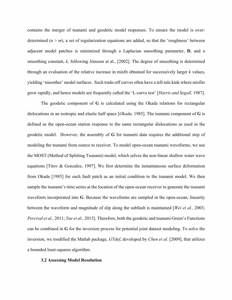
contains the merger of tsunami and geodetic model responses. To ensure the model is over-

determined (n > m), a set of regularization equations are added, so that the ‘roughness’ between

adjacent model patches is minimized through a Laplacian smoothing parameter, D, and a

smoothing constant, k, following Jónsson et al., [2002]. The degree of smoothing is determined

through an evaluation of the relative increase in misfit obtained for successively larger k values,

yielding ‘smoother’ model surfaces. Such trade-off curves often have a tell-tale kink where misfits

grow rapidly, and hence models are frequently called the ‘L-curve test’ [Harris and Segall, 1987].

The geodetic component of G is calculated using the Okada relations for rectangular

dislocations in an isotropic and elastic half space [Okada, 1985]. The tsunami component of G is

defined as the open-ocean station response to the same rectangular dislocations as used in the

geodetic model. However, the assembly of G for tsunami data requires the additional step of

modeling the tsunami from source to receiver. To model open-ocean tsunami waveforms, we use

the MOST (Method of Splitting Tsunami) model, which solves the non-linear shallow water wave

equations [Titov & Gonzalez, 1997]. We first determine the instantaneous surface deformation

from Okada [1985] for each fault patch as an initial condition to the tsunami model. We then

sample the tsunami’s time series at the location of the open-ocean receiver to generate the tsunami

waveform incorporated into G. Because the waveforms are sampled in the open-ocean, linearity

between the waveform and magnitude of slip along the subfault is maintained [Wei et al., 2003;

Percival et al., 2011; Yue et al., 2015]. Therefore, both the geodetic and tsunami Green’s Functions

can be combined in G for the inversion process for potential joint dataset modeling. To solve the

inversion, we modified the Matlab package, GTdef, developed by Chen et al. [2009], that utilizes

a bounded least-squares algorithm.

3.2 Assessing Model Resolution

Resolution assessments of finite-fault inversions commonly employ a “checkerboard test”,

as it provides a visual aid in assessing resolution [e.g. Chen et al., 2009, Moreno et al., 2010;

Romano et al., 2012; Yue et al., 2014]. It is natural that most finite-fault models will not have

enough data of the right type in the right locations to fully resolve a model over the entirety of the

model space- particularly with a finely and uniformly gridded domain. The output of a

checkerboard test can differentiate areas with good resolution, giving more confidence to model

results over the same area, and highlight areas with low resolution where modeled features may

be artifacts. The assessment of good and bad resolution stems from how well the output

checkerboard model resembles a known input- often of alternating ‘checkers’ of slip. The checker

is of a size consistent with the size of smallest feature to be modeled. While a well-resolved region

will recreate the input, a poorly resolved model will not—either the checker shape will be smeared,

or the result will be an incoherent arrangement of slip.

An alternate method of evaluating finite fault resolution is achieved by building the model

resolution matrix as a product of the model inversion process [Menke, 1989]. While the method

has been used in some past geodetic studies [Page et al., 2009; Barnhart and Lohman, 2010;

Atazori and Antonioli, 2011; Kyriakopoulos and Newman, 2016], our study is the first known

application to the tsunami wavefield.

Once the Green’s Function matrix, G, is compiled, the model resolution matrix is

determined by solving

R=[GTG + 𝝐2I]-1GTG

for the inverse problem [Backus and Gilbert, 1968; Menke, 1989]. The matrix, R, contains

information on the resolving power of the model for each parameter to be estimated and is

regulated by a weighted smoothing matrix. In an ideal case, where the model is fully resolved, R

= I, the identity matrix. In reality, perfect resolution is never truly achieved. In the imperfect case,

the diagonal components of the matrix will be equal to less than one with off-axis values indicating

the interdependence between model components. The values obtained for the model resolution

will depend on data type, location, and model, but not on the individual values of the data. The

spread of off-diagonal values per row of R is also telling to the interdependence of different model

parameters.

Past studies analyzed the limits of model resolution for the purposes of kinematic modeling

of land-based geodetic data. Non-uniform gird algorithms built to match spatial resolving power

of geodetic data to subfault size have been developed and were applied to events such as the 2004

Parkfield earthquake [Page et al., 2009] and the 1995 Antofagasta, Chile earthquake [Barnhart

and Lohman, 2010]. Areas with low resolving power dictate the necessity of coarse patches while

areas with higher resolution are resolved with a finer grid. [Atazori and Antonioli, 2011]. This

discretization reduces the influence of artifacts in the model results—unfortunate products

common in the deeper, less resolved, portion of models.

4. Results

4.1 Geodetic Resolution

While some attention has been given to the general use of the resolution matrix in subduction

zone settings for specific earthquakes [Barnhart and Lohman, 2010; Kyriakopoulos and Newman,

2016], it is also useful to look at the optimal attainable model resolution through synthetic testing.

Synthetic tests allow for the reduction of uncertainties that are present in event-based modeling by

the creation of simple and known forward models. This allows for a comparison between a result

and its synthetically-generated ‘true’ slip distribution, which is unrealistic for real-world cases.

Additionally, and pragmatically, such synthetic models are useful for understanding the limits and

options available for instrument network design.

Figure 2. Checkerboard resolution for a planar buried fault with a 15-degree dip and synthetic 3-component GNSS using static offsets. A. Checkerboard input using 30x30 km checkers of alternating 1m and 0m of pure thrust. B. Checkerboard results using a dense array of GNSS sensors (red circles) that cover the entire spatial domain. C. Checkerboard results using an array of GNSS with the same density as B. but transposed 150 km in the trench-normal (down-dip) direction. D. Same as C. but with the array transposed 300 km in the trench-normal direction.

To analyze the general subduction zone resolution problem with GNSS static offset data,

we first generate a checkerboard input and conduct a series of inversions varying data locations to

assess ability of the model to recreate the original checker pattern. The model’s spatial domain

approximates a subduction zone with a shallow dipping megathrust geometry that is discretized

into small 10x10 km subfaults. The initial checker pattern is alternated in a 30 x 30 km pattern of

between 0 and 1 m of pure thrust is used as a forward input (Figure 2a). The output of the test,

shown in Figure 2b-d is the inversion result using synthetic three-component GNSS data. The

synthetic geodetic data includes an added noise factor (5% and 10% of the horizontal and vertical

signals, respectively). Three tests are shown: (1) where geodetic data cover the up-dip spatial

domain essentially to the trench (spaced every 25 km down-dip and 33 km along-strike; Figure

2b); (2) where geodetic data stops 150 km from the trench (Figure 2c); and (3) where geodetic data

doesn’t start until 300 km from the trench (Figure 2d).

In each case, the checkerboard output illustrates a loss of model resolution as the distance

between data and model parameters increases. In Figure 2b, a case possibly representing a rich

seafloor geodetic array, the checkerboard pattern is well recreated throughout almost all of the

spatial domain. A small smearing of the checkers occurs down-dip where resolution is reduced

due to increased distance between the surface data and the model interface at depth. Figures 2c

and 2d show the resolution as the GNSS dataset locations are transposed 150 and 300 km in the

down-dip direction. These distances are equivalent to the coast-trench distances exhibited in some

parts of the Cascadia and Alaskan examples shown in Figure 1. In both cases, the near-trench

resolution is lost as the data distance increases, resulting in an incoherent fault plane solution where

the checker pattern is no longer recreated. Checker coherence is lost in Figure 2c after data-model

distances exceed 50 km. Figure 2d corroborates this observation but with the added effects of a

larger vertical distance between source and receiver (due to increasing fault depth), leading to a

larger reduction in resolution over the entire fault geometry. The overall trend shown in Figure 2

is a loss in resolution via smeared checkers with the removal of data in the trenchward direction.

For the fault geometry used, this loss in checker recreation occurs about 50 km away from the

closest data. While the checker shape is lost as data is removed, model results can still create slip

distributions that, without a prior knowledge of the slip input, could falsely be confused with a

reliable result.

The model resolution matrix, R, provides an additional metric to assess fault recoverability

and more importantly, to compare the degree of resolution between different models due to a range

of varying factors without relying on a synthetic slip distribution as a known input. Using a trench-

normal transect of the first 100 km of the subduction zone geometry used in Figure 2, we assess

the effect that fault geometry, GNSS data distance, and subfault discretization has on the model

resolution. Each diagonal component, i, of the square matrix R, represents the model resolution of

an individual subfault along the transect. Figure 3 shows how fault depth and data distance affect

model resolution. The influence between fault depth and model resolution is described by the black

line labeled “0 km”. In this case, instruments exist over the entire transect, similarly to the data

dense case in Figure 2. Starting at the trench and extending for the first 20 km laterally along the

profile, the diagonals of R approach a value of one, indicating high resolution. This region

represents the shallow near-trench environment and the depth between the fault plane and GNSS

instruments varies between 0 and 5 km. As the transect distance increases to 40 km, the depth

between the surface and the fault reaches 10 km, and the model resolution is halved (Ri = 0.5). At

75 km from the trench, the fault depth increases to 20 km and the resolution decays further (Ri =

0.28). Along the transect, the GNSS data density remains constant, but the resolution decreases

with to the increasing depth. The results shown in Figure 3 assume a constant fault dip of 15º,

however a change in dip, which affects the fault depth, also affects resolution as shown in Figure

S1.

Figure 3. Transect in the trench-normal direction for the first 100 km of a shallowly dipping interface, approximating a subduction zone. Model resolution in the trench-normal direction is plotted for 10 scenarios (colored lines). Each scenario transposes the location of the nearest GNSS data in the down-dip direction.

The effect of data location on the model resolution is described by the colored lines in

Figure 3. Each line represents a different model result with the color indicating the distance of the

closest GNSS data with respect to the location of the trench. The trend governing the data location

shows that when data coverage is dense and extends to the trench, the diagonal components of R

approach one (and decay mainly due to depth increases). As the data coverage in the near trench

environment decreases, as evidenced when nearest sites grow from 20 to 60 km away, the

corresponding diagonal components of R decrease. In the case where the only data available is

Mod

el R

esol

utio

n

Trench−Normal Distance [km]

Nearest GNSS to Trench [km]

20 40 60 80 100 120 140 160 180

0.2

0.4

0.6

0.8

1.0

Faultdip = 15 °

50 patches0-30 km depth

20 k

m

60 km 100 km 140 km180 km

0 km

0 20 40 60 80 100

much further from the trench, 100 km or more, the diagonal components of R approach zero.

Resolution is lost, to a greater degree, due to increasing distance between parameter and receiver

in the trench-normal direction than due to the same distance offsetting source and receiver purely

from an increase in depth.

The size of subfaults on the discretized fault plane also effects the model resolution. When

data locations are limited, a method that raises the values of R is to increase the size of fault patches

used in the inversion to satisfy the level of data availability. Figure 4 illustrates the effect that the

change in fault discretization has on the model resolution. For each case, the fault plane’s dip and

the amount of data available are held constant, but the number of subfaults changes. The fewer

subfaults used, the larger each patch is, increasing the overall model resolution. In cases where

data is not present over the entire model space (Figure 4b), the subfault size can be increased,

yielding a better resolution in data limited regions. However, while an increase in subfault size

can increase resolution, the ability to model fine scaled features is reduced.

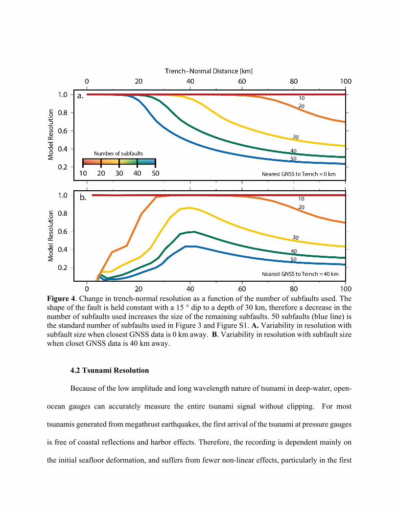
Figure 4. Change in trench-normal resolution as a function of the number of subfaults used. The shape of the fault is held constant with a 15 ° dip to a depth of 30 km, therefore a decrease in the number of subfaults used increases the size of the remaining subfaults. 50 subfaults (blue line) is the standard number of subfaults used in Figure 3 and Figure S1. A. Variability in resolution with subfault size when closest GNSS data is 0 km away. B. Variability in resolution with subfault size when closet GNSS data is 40 km away.

4.2 Tsunami Resolution

Because of the low amplitude and long wavelength nature of tsunami in deep-water, open-

ocean gauges can accurately measure the entire tsunami signal without clipping. For most

tsunamis generated from megathrust earthquakes, the first arrival of the tsunami at pressure gauges

is free of coastal reflections and harbor effects. Therefore, the recording is dependent mainly on

the initial seafloor deformation, and suffers from fewer non-linear effects, particularly in the first

1000 km of wave propagation [Rabinovich and Eble, 2015]. As such, many studies treat the

tsunami as a linear extension of the slip along the fault [Wei et al., 2003; Percival et al., 2011; Yue

et al., 2015]. We use synthetically generated tsunami waveforms for an array of theoretical

pressure gauge locations as well as established DART gauge locations from the National Data

Buoy Center to assess the same model resolution parameters as was shown for the geodetic data

in the preceding section.

Figure 5. The model resolution for each subfault using only an open-ocean tsunami dataset and one gauge, located at Cartesian (-400, -275). A. Inversion using the full highlighted waveform from gauge 1. The observed waveform, as well as the Green’s functions for subfaults a, b, and c are highlighted. B. Inversion using a windowed portion of the time series observed at gauge 1. Windowed portion incorporated into inversion is the observed waveform is highlighted in red. The same Green’s functions as shown in panel A. are also shown, but highlighting the windowing process. Note how Green’s function “c” is not included in the window, leading to the poor resolution.

The synthetic pressure gauges from which waveforms are calculated are located between 500

and 800 km seaward from the source, simulating typical distances found in some recent studies

using tsunami data for source inversions [e.g. An et al., 2014; Williamson et al., 2017; Adriano et

al., 2018]. Here, we use the same shallow-dipping and planar fault geometry as used in the geodetic

analysis (Figures 2 and 3), and a 30x30 km cell size. The subfault size is increased to limit

computation costs but within range of subfault sizes used in past tsunami inversion studies [e.g.

Fujii et al., 2011; Heidarzadeh et al., 2016; Yoshimoto et al., 2016] and within the boundaries of

a longwave approximation (Figure S2). We then assess resolution using synthetically generated

waveforms and the locations of three currently deployed pressure gauges along the Peru-Chile

trench.

In a synthetic case, observed open-ocean tsunami waveforms include the contribution from

slip on each subfault. Figure 5 shows the model resolution using one synthetic gauge and the entire

recorded waveform with a sample frequency of 60 s and an added noise equaling 10% of the

signal’s amplitude. In this end member case, one waveform is sensitive to displacement from all

of the subfaults with an uninhibited propagation path, therefore the entire fault plane has nearly

perfect resolution, where R approaches the identify matrix, I. Likewise, the checkerboard tests

using the same dataset (Figure S3) appears to replicate the original checker pattern. However, it is

important to note that this well-resolved result is an idealized scenario and does not include effects

that are seen in real tsunami signals, leading to a physically improbable result.

A real tsunami signal will often include effects that are difficult to adequately model through

linear approximations. One of the largest sources of uncertainty includes the loss of energy due to

coastal reflections which affects the latter part of the wave train at open-ocean gauges and interacts

with the arrival of more distal parts of the tsunami source, convoluting the overall signal. For the

purposes of illustrating an ideal case, these effects are ignored in Figure 5a but included in Figure

5b. Windowing, or cropping the inverted time series to only include a subset of the data is an

extremely common practice. Typically, only the first one to two wavelengths of recorded tsunami

at any gauge are used in the inversion [e.g. An et al, 2014; Gusman et al, 2014; Li et al., 2016;

Williamson et al., 2017; Adriano et al., 2018]. Later phases are discarded to reduce the impact of

un-modeled or complex effects. Unfortunately, at times useful primary fault slip information is

also discarded with these data.

Figure 5 shows the effects of windowing the time series by only incorporating the first few

wavelengths of the waveform into the inversion and calculating the model resolution matrix. After

the latter part of the time series has been removed the model is only sensitive to a subset of the

spatial domain. Therefore, the location of the gauge with respect to the fault plane affects the

resolution. In this case, the subfault generated Green’s Functions containing waves with the

earliest travel-time to the gauge will maintain high resolution, as they are retained in the time series

window. In contrast, waveforms that are sensitive to subfaults further away may no longer be

included when using short windowed observations. Checkerboard tests using windowed tsunami

waveforms also highlight the variability in resolution through a loss in the coherent checker pattern

(Figure S3). If the windowing techniques used are more restrictive (more data is removed) then an

even larger part of the model space may lose resolution. The degree of windowing in highly

dependent on the propagation path of the tsunami.

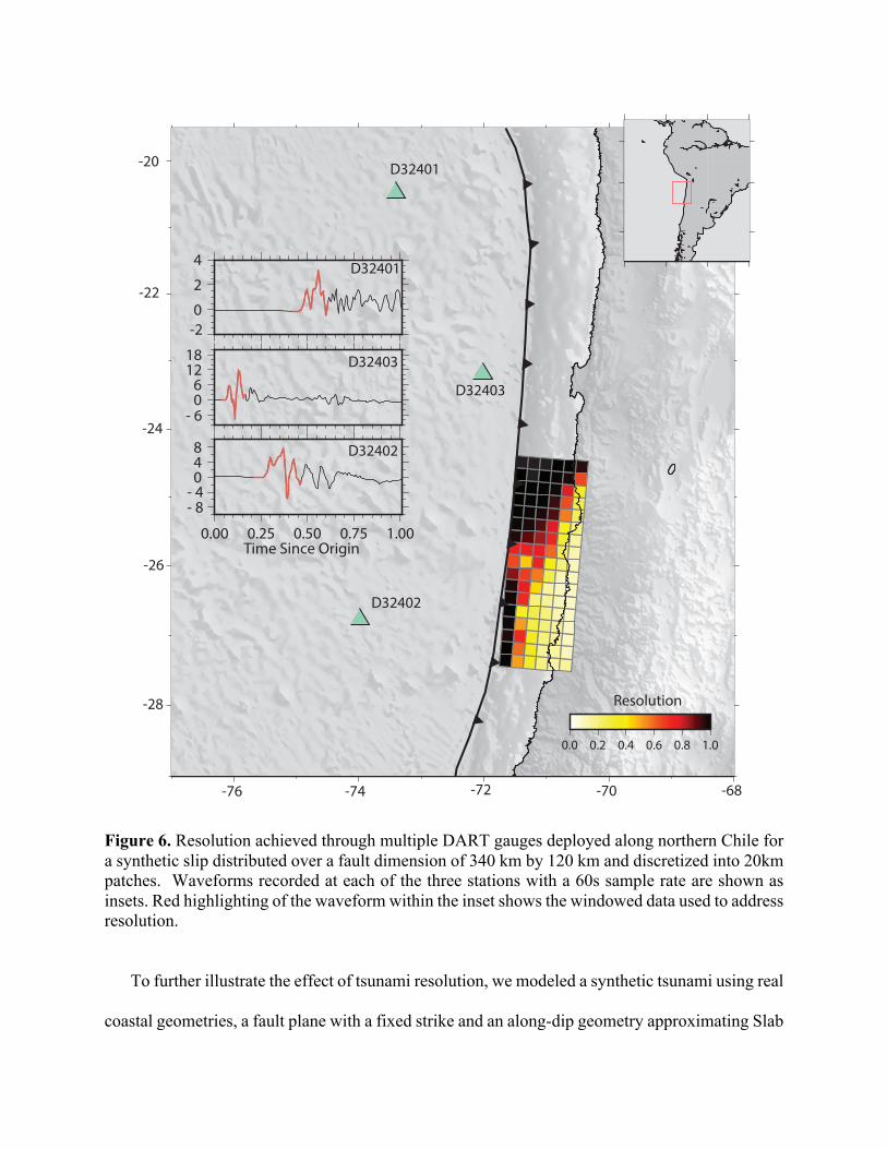
Figure 6. Resolution achieved through multiple DART gauges deployed along northern Chile for a synthetic slip distributed over a fault dimension of 340 km by 120 km and discretized into 20km patches. Waveforms recorded at each of the three stations with a 60s sample rate are shown as insets. Red highlighting of the waveform within the inset shows the windowed data used to address resolution.

To further illustrate the effect of tsunami resolution, we modeled a synthetic tsunami using real

coastal geometries, a fault plane with a fixed strike and an along-dip geometry approximating Slab

0.0 0.2 0.4 0.6 0.8 1.0

D32401

D32402

Resolution

-20

-22

-24

-26

-28

-74 -72 -70 -68-76

D32401

D32402

024

048

0.00 0.25 0.50 0.75 1.00

06

1218

-2

- 6

- 4- 8

Time Since Origin

D32403

D32403

1.0 [Hayes et al., 2012], and locations of three currently deployed DART gauges along Northern

Chile in Figures 6. In Figure 7, we also show the model resolution attainable for an extension of

the fault geometry using the Centro Sismológico Nacional (CSN) current network of GNSS

sensors as listed in Báez et al. (2018) and the combined resolution from jointly using both datasets.

Chile is highlighted as an example area because of the region’s large array of nearby DART

gauges, including newer, near-trench DART 4G instruments, its three recent large (M8+)

megathrust earthquakes in the past decade (2010 Mw 8.8 Maule, 2014 MW 8.1 Iquique, and 2015

Mw 8.3 Illapel earthquakes) and recent studies from the region focusing on rapid source evaluation

for earthquake and tsunami early warning [Báez et al., 2018; Crowell et al., 2018] making it an

interesting source region for resolution studies.

In Figure 6, a synthetic tsunami with slip over a 340 km long fault is modeled and sampled at

three DART gauges. The windowing of each of the waveforms limits the influence of reflections

from the nearby coastline but also reduces resolution over some parts of the modeled space. Lower

resolution occurs on parts of the fault that would arrive at gauges later. In the case of the three

gauges shown in Figure 6, the area with the lowest resolution is in the central and down-dip portion

of the fault geometry.

If the extent of tsunamigenic slip increases, as is shown in Figure 7, the area of lower resolution

increases. This poorly resolved area has a much later arrival time at the DART sensors and outside

of the windowed part included in the inversion. The sensitivity to slip occurring within the central

portion of the slip reduces as the signal is mixed with reflected waveforms from neighboring fault

patches. The total size of the feature to be resolved, rather than the distance to the open-ocean

sensors, affects the model resolution. While resolution can be increased by including more DART

gauge data at different enough azimuths from the source to have windowed time series that are

sensitive to different portions of the fault, open-ocean data is typically spaced hundreds of

kilometers apart. This loss in model resolution is a departure from the geodetic resolution results

where slip of any size can be resolved so long as there is a dense array of localized instruments.

The model resolution for the same region, but by using the current catalog of GNSS sensors

along the Chilean coast, also shown in Figure 7, highlights similar findings to the synthetic

simulations shown earlier in this study. As the distances between the GNSS station locations and

the model parameter being solved for increase, the model resolution decreases. This is best shown

by the coastal GNSS gauges around 26° S latitude where model resolutions greater than 0.5 extend

up to 60 km offshore, but resolution towards the south at 27° S latitude remains poor due to a

sparser local network. The complimentary behavior of joint GNSS and tsunami inversions in terms

of achievable model resolution is included in the furthest right panel of Figure 7 where we plot the

model resolution for a joint inversion. Here, high model resolution is maintained throughout the

model space.

Figure 7. Resolution achieved through various datasets. A. Model resolution using only three DART gauges (triangles) deployed along northern Chile over a fault dimension of 760 km by 120 km and discretized into 20km patches. Waveforms recorded at each of the three stations with a 60s sample rate are shown as insets. Red highlighting of the waveform within the inset shows the windowed data used to address resolution. B. Model resolution using only GNSS from CSN’s geodetic network. White squares indicate instrument locations; C. Model resolution using both GNSS and DART gauges together.

4.3 Resolution Spread

Just as prior work has constrained the size of resolvable features for geodetic datasets [Page

et al., 2009; Barnhart and Lohman, 2010; Atzori and Antonioli, 2011], tsunami data can be

assessed per model to determine the scale of resolvable features. The spread of values on the off-

diagonal components of R indicate the interdependence of adjacent parameters. For finite-fault

studies, this amounts to the dependence of the subfault analyzed to the slip on the surrounding

subfaults. For a fully resolved parameter, there is no interdependence with surrounding subfaults.

0.0

0.2

0.4

0.6

0.8

1.0

D32401

D32402

D32403

Resolution

A.

024

048

0.00 0.25 0.50 0.75 1.00

06

1218

-2

- 6

- 4- 8

-76 -74 -72 -70 -68

-20

-22

-24

-26

-28

-30

Time Since Origin

D32402

D32403

D32401

D32401

D32402

D32403

B.

D32401

D32402

D32403

C.

But for a poorly resolved parameter, the interdependence will extend over a wide area around the

subfault in question [Funning et al., 2007]. This limits the size of features in the slip model that

can be resolved to the size of the spread.

Rather than exhaustively analyze the interdependence of each subfault to its surroundings,

a general resolution spread can be easily derived and applied to each subfault. The use of the

resolution spread parameter, ri, quantitatively indicates the smallest resolvable feature in the model

through:

𝑟+ =𝐿𝑅+

Where L is the length scale of the subfault and Ri is the diagonal component of the matrix

corresponding to the ith parameter [Funning et al., 2007]. A perfectly resolved model can determine

features down to the size of the discretized subfault. A poorly resolved area will only be able to

resolve coarser features. The use of a resolution spread parameter to determine the length scale of

the smallest resolvable features can easily replace the sometimes exhaustive use of multiple

checkerboard tests with varying checker dimensions.

Figure 8. Resolution spread, ri, achieved from the A. DART only, B. GNSS only, and C joint dataset inversions highlighted in Figure 7. The greater the spread, the less detail that can be resolved. The smallest spread value possible is equal to the patch size of 20 km. The color scale for upper extent of spread saturates at 80 km.

The resolution spread parameter is applied to the the scenario discussed in Figure 7 and

presented in Figure 8. The best resolution spread is close to the subfault size of 20 km, indicating

an R value near 1 for those patches. However, in the areas with lower resolution, the smallest

resolvable feature is a much coarser 80 km or larger. Just as shown in Figure 7, the best achievable

resolution spread (the smallest value) occurs when both tsunami and GNSS datasets are combined

due to their complementary nature. The best resolution for a GNSS-only dataset is only found

close to the coast through on land, while the best resolution for a tsunami-only dataset is found

offshore and further from land.

20

40

60

D32401

D32402

D32403

A.

Spread [km]

D32401

D32402

D32403

B.

D32401

D32402

D32403

C.

-20

-22

-24

-26

-28

-30-74 -72 -70 -68

5. Discussion

The effect of data location on model resolution is indicative of the real problem of offshore

data sparsity at subduction zones. The sometimes vast distances between seismic slip and

coastlines shown in Figure 1 reiterates the need for offshore sensitive datasets. In all of the four

highlighted regions, the distance between the coastline and the trench is large enough that the

trench environment will have reduced resolution, as described in Figure 3. Even with coarser

subfault discretization, distal locations such as the trenchward extent of the Cascadia subduction

zone, almost 300 km away from the coastline, are too far to adequately resolve from static GNSS

displacements alone. Many recent megathrust events, including the 2004 Mw 9.1 Sumatra

earthquake, the 2006 Mw 8.3 Kuril Island earthquakes, and the 2011 Mw 9.1 Tohoku earthquake,

have ruptured exclusively offshore. While seafloor geodetic data such as absolute pressure sensors

and GPS-A exists in some regions, it is not yet widespread enough to be utilized in many global

rupture studies. In the absence of seafloor geodetic data, tsunami waveform datasets provide much

improved resolution over this environment.

Model resolution using tsunami sensitive datasets is not dependent on fault geometry, so

long as there is sufficient seafloor deformation to generate a tsunami. The distance between the

tsunami source and open-ocean receiver also does not have a strong influence on resolution past

reaching the instrument detection limit. However, the extent of the rupture area and data processing

affects the total model resolution. While tsunami datasets lack resolution on land, and geodetic

datasets largely are insensitive to far offshore slip, the increasingly popular joint inversion of both

datasets provides a potentially rich dataset that can be used to better understand slip over the entire

megathrust seismogenic zone. This can refine our understanding of where we do, and do not see

slip, particularly in the shallow, and generally stably sliding portion of the megathrust [Lay et al.,

2012]. It is important to point out that earthquake ruptures rarely behave as fully offshore or fully

under-land events. Both datasets, geodetic and tsunami, will be sensitive to at least a small portion

of the rupture domain. Outside of each dataset’s region of sensitivity, resolution does not abruptly

end but does become limited.

In earthquake rupture studies, where the ‘true’ slip distribution is unknown, one widely

used metric for determining model correctness is data misfit. A poorly resolved model may appear

to adequately fit the data, but will not necessarily be correct. In a case with poor model resolution,

disparate finite-fault slip solutions with little in common can fit the observed data equally well

[e.g. Olsen and Apsel, 1982; Beresnev, 2003]. This false equivalence between model fit and model

correctness is a large threat for subduction zone modeling where oftentimes the model resolution

varies over the spatial domain. Even though a ‘true’ slip distribution will never be known,

knowledge of the model resolution to avoid putting confidence in q-space solutions is key. These

null-space solutions, particularly when they look physically feasible in source inversions, run the

risk of being interpreted as real features of the model. Solutions in these low-resolution zones can

vary from incoherent patterns to large, improbably scaled levels of slip, all of which will have no

bearing on the overall fit of the data. For studies focusing on real events with unknown sources,

this possible inaccuracy of null-space solutions as near-trench or unresolvable slip directly impacts

assessments of seismic and tsunami hazard. This is problematic both for warnings made in real-

time and post-event studies assessing the likelihood of shallow strain accumulation and release.

Without careful consideration of model resolution, finite-fault results incorporating data-

insensitive zones of slip can easily shape our understanding of subduction zone seismicity. It is

common following large earthquakes to assess the change in stress in the area surrounding the

rupture zone [Luttrell et al., 2011] as well as how modeled slip behavior affects the presence of

seismic gaps [Lorito et al., 2011; Moreno et al., 2012; Métois et al., 2016] with the aid of slip

models. These models, without proper data handling, could be potentially dangerous if used by

non-experts for regional interpretation of seismic or tsunami hazard.

6. Conclusion

Many studies integrate multiple new datasets in finite-fault source inversion to allow for

better understanding of slip distribution along subduction zones. With the addition of offshore

datasets, such as open-ocean tsunami waveforms, it is important to understand not only the benefits

the data provides to a model, but also the limitations. This is partially achieved by analyzing how

the sensitivity of tsunami and geodetic datasets vary with location and treatment. Geodetic data is

highly sensitive to deformation occurring in its immediate (within 50 km) vicinity. However

special care needs to be given to modeling megathrust rupture with GNSS data when a) the depth

between instrument and fault plane exceeds 30 km and b) the distance between instrument and

offshore slip exceeds 40 km. In order to model slip in the near-trench environment with geodetic

data, either offshore GPS-acoustic or land proximal to the rupture zone should be employed to

maintain resolution. In conjunction with the use of a nearby and sensitive dataset, the scale of fault

patches used in finite-fault modeling needs to be coarse enough to reduce the impact of slip

artifacts. This can be quantified by analyzing the resolution spread which will vary as subfault size

changes.

Open-ocean tsunami data provide resolution offshore down to 20 km patches when data is

available, and not interfered by coastal reflections. Resolution is greatly reduced by necessary

windowing, which is employed to minimize un-modeled effects can, in the process, discard useful

information about slip. As the window is reduced, so is the area on the fault plane that each open-

ocean gauge is sensitive to. Additional care should be used in the treatment of time series data

from gauges located more than 1000 km away from the source zone, as the accumulation of errors

in modeling the bathymetry, wave dispersion, and elastic loading can interfere with the model

solution [Allgeyer & Cummins, 2014; Watada et al., 2014]. A very positive attribute of the tsunami

dataset is that despite the limited number of gauges available, only a couple of well-placed sites

are necessary to obtain well-resolved fault plane solutions over a large area, a number far lower

than the number of GNSS stations normally required on-land, while still missing much of the

offshore action. If no coasts were in play, only a single open-ocean tsunami station would be

necessary.

The understanding of where a model is well resolved is just as important as understanding

where it is not. Poorly resolved areas which may lack data, should be analyzed with the

understanding that the scale of features presented in the inversion may not be robust. Through the

use of multiple different datasets, particularly through the inclusion of both land sensitive and

seafloor sensitive data, a comprehensive understanding of slip from the shallow near-trench

environment through the entire seismogenic interface may be achieved. The use of both geodetic

and tsunami datasets as highlighted in this study work as complements, where geodetic data

quickly loses resolution offshore, tsunami data fill in the gap. Where tsunami data cannot constrain

deformation occurring inland, geodetic data is often well suited.

Acknowledgments This research was supported through State Funds through Georgia Tech to AVN. Synthetic

data are generated through the Matlab suite GTdef and the MOST tsunami propagation code. Input data for synthetic GNSS tests and tsunami Green’s Function data are available as a supplemental directory. Source codes for GTdef are available through Github upon request from the corresponding author.

References Adriano, B., Y. Fujii, S. Koshimura, E. Mas, A. Ruiz-Angulo, M. Estrada (2018), Tsunami Source

Inversion Using Tide Gauge and DART Tsunami Waveforms of the 2017 Mw8. 2 Mexico

Earthquake, Pure and Applied Geophysics, 1-14. Doi: 10.1007/s00024-017-1760-2

Allgeyer, S., & Cummins, P. (2014). Numerical tsunami simulation including elastic loading and

seawater density stratification. Geophysical Research Letters, 41(7), 2368-2375.

An, C., I. Sepúlveda, PLF. Liu (2014), Tsunami source and its validation of the 2014 Iquique,

Chile Earthquake, Geophys. Res. Lett., 41, 3988–3994, doi:10.1002/2014GL060567.

Atzori, S., A. Antonioli (2011), Optimal fault resolution in geodetic inversion of coseismic

data, Geophysical Journal International, 185(1), 529-538, doi: 10.1111/j.1365-

246X.2011.04955.x.

Backus, G., & Gilbert, F. (1968). The resolving power of gross earth data. Geophysical Journal of

the Royal Astronomical Society, 16(2), 169-205.

Báez, J. C., Leyton, F., Troncoso, C., del Campo, F., Bevis, M., Vigny, C., ... & Blume, F. (2018).

The Chilean GNSS Network: Current Status and Progress toward Early Warning

Applications. Seismological Research Letters.

Barnes, C. R., Best, M. M., Johnson, F. R., Pautet, L., and Pirenne, B. (2013), Challenges, benefits,

and opportunities in installing and operating cabled ocean observatories: Perspectives from

NEPTUNE Canada. IEEE Journal of Oceanic Engineering, 38(1), 144-157.

Barnhart, W. D., R. B. Lohman (2010), Automated fault model discretization for inversions for

coseismic slip distributions, Journal of Geophysical Research: Solid Earth, 115(B10). Doi:

10.1029/2010JB007545

Beresnev, I. A. (2003). Uncertainties in finite-fault slip inversions: to what extent to believe? (a

critical review). Bulletin of the Seismological Society of America, 93(6), 2445-2458.

Doi: https://doi.org/10.1785/0120020225

Bernard, E. N., & Meinig, C. (2011, September). History and future of deep-ocean tsunami

measurements. In OCEANS 2011 (pp. 1-7). IEEE.

Bernard, E. N., H. O. Mofjeld, V. Titov, C. E. Synolakis, F. I. González, F. I. (2006), Tsunami:

scientific frontiers, mitigation, forecasting and policy implications. Philosophical

Transactions of the Royal Society of London A: Mathematical, Physical and Engineering

Sciences, 364(1845), 1989-2007.

Bernard, E. N., & Titov, V. V. (2015), Evolution of tsunami warning systems and

products. Philosophical Transactions of the Royal Society of London A: Mathematical,

Physical and Engineering Sciences, 373(2053), 20140371

Blewitt, G., Kreemer, C., Hammond, W. C., Plag, H. P., Stein, S., & Okal, E. (2006). Rapid

determination of earthquake magnitude using GPS for tsunami warning

systems. Geophysical Research Letters, 33(11).

Chadwick Jr, W. W., S. L. Nooner, D. A. Butterfield, and M. D. Lilley (2012). Seafloor

deformation and forecasts of the April 2011 eruption at Axial Seamount, Nature

Geoscience 5, (7): 474-477.

Chen, T., A. V. Newman, L, Feng, H. M. Fritz (2009), Slip Distribution from the 1 April 2007

Solomon Islands Earthquake: A Unique Image of Near-Trench Rupture, Geophys. Res.

Lett., 36, L16307, doi:10.1029/2009GL039496

Crowell, B. W., Melgar, D., & Geng, J. (2018a). Hypothetical Real-Time GNSS Modeling of the

2016 M w 7.8 Kaikōura Earthquake: Perspectives from Ground Motion and Tsunami

Inundation Prediction. Bulletin of the Seismological Society of America.

Crowell, B. W., Schmidt, D. A., Bodin, P., Vidale, J. E., Baker, B., Barrientos, S., & Geng, J.

(2018b). G-FAST earthquake early warning potential for great earthquakes in

Chile. Seismological Research Letters, 89(2A), 542-556.

Fujii, Y., Satake, K., Sakai, S. I., Shinohara, M., & Kanazawa, T. (2011). Tsunami source of the

2011 off the Pacific coast of Tohoku Earthquake. Earth, planets and space, 63(7), 55.

Funning, G. J., B. Parsons, T. J. Wright (2007), Fault slip in the 1997 Manyi, Tibet earthquake

from linear elastic modelling of InSAR displacements. Geophysical Journal

International, 169(3), 988-1008. Doi: 10.1111/j.1365-246X.2006.03318.x.

Gagnon, K., C. D. Chadwell, and E. Norabuena (2005), Measuring the onset of locking in the Peru-

Chile trench with GPS and acoustic measurements, Nature, 434(7030), 205-208,

doi:http://dx.doi.org/10.1038/nature03412.

Geist, E. L. (2002). Complex earthquake rupture and local tsunamis. Journal of Geophysical

Research: Solid Earth, 107(B5).

Goda, K., Mai, P. M., Yasuda, T., & Mori, N. (2014). Sensitivity of tsunami wave profiles and

inundation simulations to earthquake slip and fault geometry for the 2011 Tohoku

earthquake. Earth, Planets and Space, 66(1), 105.

Gusman, A. R., S. Murotani, K. Satake, M. Heidarzadeh, E. Gunawan, S. Watada, B. Schurr,

(2015), Fault slip distribution of the 2014 Iquique, Chile, earthquake estimated from ocean-

wide tsunami waveforms and GPS data. Geophys. Res. Lett., 42: 1053–1060.

doi:10.1002/2014GL062604.

Gusman, A. R., Mulia, I. E., & Satake, K. (2017). Optimum sea surface displacement and fault

slip distribution of the 2017 Tehuantepec earthquake (Mw 8.2) in Mexico estimated from

tsunami waveforms. Geophysical Research Letters. Doi: 10.1002/2017GL076070

Hayes, G. P., Wald, D. J., & Johnson, R. L. (2012). Slab1. 0: A three-dimensional model of global

subduction zone geometries. Journal of Geophysical Research: Solid Earth, 117(B1).

Harris, R. A., P. Segall (1987), Detection of a locked zone at depth on the Parkfield, California,

segment of the San Andreas Fault, J. Geophys. Res., 92(B8), 7945–7962,

doi:10.1029/JB092iB08p07945.

Heidarzadeh, M., S. Murotani, K. Satake, T. Ishibe, A. R. Gusman (2016), Source model of the 16

September 2015 Illapel, Chile, Mw 8.4 earthquake based on teleseismic and tsunami data,

Geophys. Res. Lett., 43, 643–650, doi:10.1002/2015GL067297.

Jónsson, S., Zebker, H., Segall, P., & Amelung, F. (2002). Fault slip distribution of the 1999 M w

7.1 Hector Mine, California, earthquake, estimated from satellite radar and GPS

measurements. Bulletin of the Seismological Society of America, 92(4), 1377-1389.

Kyriakopoulos, C., A. V. Newman (2016), Structural asperity focusing locking and earthquake

slip along the Nicoya megathrust, Costa Rica, Journal of Geophysical Research: Solid

Earth, 121(7), 5461-5476. Doi: 10.1002/2016JB012886

Lay, T., Kanamori, H., Ammon, C.J., Koper, K.D., Hutko, A.R., Ye, L., Yue, H. and Rushing,

T.M., 2012. Depth-varying rupture properties of subduction zone megathrust

faults. Journal of Geophysical Research: Solid Earth, 117(B4).

Li, S., Moreno, M., Bedford, J., Rosenau, M. and Oncken, O., 2015. Revisiting viscoelastic effects

on interseismic deformation and locking degree: A case study of the Peru-North Chile

subduction zone. Journal of Geophysical Research: Solid Earth, 120(6), pp.4522-4538.

Li, L., K. F. Cheung, H. Yue, T. Lay, Y. Bai (2016), Effects of dispersion in tsunami Green's

functions and implications for joint inversion with seismic and geodetic data: A case study

of the 2010 Mentawai Mw 7.8 earthquake, Geophysical Research Letters, 43(21). Doi:

10.1002/2016GL070970

Lorito, S., Romano, F., Atzori, S., Tong, X., Avallone, A., McCloskey, J., ... & Piatanesi, A.

(2011). Limited overlap between the seismic gap and coseismic slip of the great 2010 Chile

earthquake. Nature Geoscience, 4(3), 173.

Luttrell, K. M., Tong, X., Sandwell, D. T., Brooks, B. A., & Bevis, M. G. (2011). Estimates of

stress drop and crustal tectonic stress from the 27 February 2010 Maule, Chile, earthquake:

Implications for fault strength. Journal of Geophysical Research: Solid Earth, 116(B11).

Meinig, C., Stalin, S. E., Nakamura, A. I., González, F., & Milburn, H. B. (2005, September).

Technology developments in real-time tsunami measuring, monitoring and forecasting.

In OCEANS, 2005. Proceedings of MTS/IEEE (pp. 1673-1679). IEEE.

Melgar, D., Crowell, B. W., Geng, J., Allen, R. M., Bock, Y., Riquelme, S., ... & Ganas, A. (2015).

Earthquake magnitude calculation without saturation from the scaling of peak ground

displacement. Geophysical Research Letters, 42(13), 5197-5205.

Melgar, D., W. Fan, S. Riquelme, J. Geng, C. Liang, M. Fuentes, et al., (2016), Slip segmentation

and slow rupture to the trench during the 2015, Mw8. 3 Illapel, Chile

earthquake, Geophysical Research Letters, 43(3), 961-966. Doi: 10.1002/2015GL067369

Menke, W. (1989), Geophysical Data Analysis: Discrete Inverse Theory, Academic, San Diego,

Calif.

Métois, M., Vigny, C., & Socquet, A. (2016). Interseismic coupling, megathrust earthquakes and

seismic swarms along the Chilean subduction zone (38–18 S). Pure and Applied

Geophysics, 173(5), 1431-1449.

Moreno, M., M. Rosenau, O. Oncken (2010), 2010 Maule earthquake slip correlates with pre-

seismic locking of Andean subduction zone, Nature, 467(7312), 198-202. Doi:

10.1038/nature09349

Moreno, M., Melnick, D., Rosenau, M., Baez, J., Klotz, J., Oncken, O., ... & Socquet, A. (2012).

Toward understanding tectonic control on the Mw 8.8 2010 Maule Chile earthquake. Earth

and Planetary Science Letters, 321, 152-165.

Mungov, G., Eblé, M., & Bouchard, R. (2013). DART® tsunameter retrospective and real-time

data: A reflection on 10 years of processing in support of tsunami research and

operations. Pure and Applied Geophysics, 170(9-10), 1369-1384.

Newman, A. V. (2011). Hidden depths. Nature, 474(7352), 441.

Okada, Y., (1985). Surface deformation due to shear and tensile faults in a half-space. Bulletin of

the seismological society of America, 75(4), pp.1135-1154.

Olson, A. H., R.J. Apsel, R. J. (1982), Finite faults and inverse theory with applications to the 1979

Imperial Valley earthquake. Bulletin of the Seismological Society of America, 72(6A),

1969-2001.

Page, M. T., S. Custódio, R. J. Archuleta, J. M. Carlson (2009), Constraining earthquake source

inversions with GPS data: 1. Resolution-based removal of artifacts, Journal of Geophysical

Research: Solid Earth, 114(B1). Doi: 10.1029/2007JB005449

Percival, D. B., Denbo, D. W., Eblé, M. C., Gica, E., Mofjeld, H. O., Spillane, M. C., ... & Titov,

V. V. (2011). Extraction of tsunami source coefficients via inversion of DART buoy

data. Natural hazards, 58(1), 567-590.

Percival, D. B., Denbo, D. W., Eblé, M. C., Gica, E., Huang, P. Y., Mofjeld, H. O., ... & Tolkova,

E. I. (2015). Detiding DART® buoy data for real-time extraction of source coefficients for

operational tsunami forecasting. Pure and Applied Geophysics, 172(6), 1653-1678.

Rabinovich, A. B., & Eblé, M. C. (2015). Deep-ocean measurements of tsunami waves. Pure and

Applied Geophysics, 172(12), 3281-3312.

Romano, F., A. Piatanesi, S. Lorito, N. D'agostino, K. Hirata, et al (2012), Clues from joint

inversion of tsunami and geodetic data of the 2011 Tohoku-oki earthquake, Scientific

reports, 2, 385. Doi: 10.1038/srep00385

Ruhl, C. J., Melgar, D., Grapenthin, R., & Allen, R. M. (2017). The value of real-time GNSS to

earthquake early warning. Geophysical Research Letters, 44(16), 8311-8319.

Satake, K. (1987). Inversion of tsunami waveforms for the estimation of a fault heterogeneity:

Method and numerical experiments. Journal of Physics of the Earth, 35(3), 241-254.

Thomson, R., Fine, I., Rabinovich, A., Mihály, S., Davis, E., Heesemann, M., & Krassovski, M.

(2011). Observation of the 2009 Samoa tsunami by the NEPTUNE-Canada cabled

observatory: Test data for an operational regional tsunami forecast model. Geophysical

Research Letters, 38(11).

Tilmann, F., Y. Zhang, M. Moreno, J. Saul, F. Eckelmann, M. Palo, Z. Deng et al. "The 2015

Illapel earthquake, central Chile: A type case for a characteristic

earthquake?." Geophysical Research Letters 43, no. 2 (2016): 574-583.

Titov, V. V., F. I. Gonzalez. Implementation and testing of the method of splitting tsunami (MOST)

model. US Department of Commerce, National Oceanic and Atmospheric Administration,

Environmental Research Laboratories, Pacific Marine Environmental Laboratory, 1997.

Watada, S., Kusumoto, S., & Satake, K. (2014). Traveltime delay and initial phase reversal of

distant tsunamis coupled with the self-gravitating elastic Earth. Journal of Geophysical

Research: Solid Earth, 119(5), 4287-4310.

Wei, Y., Cheung, K. F., Curtis, G. D., & McCreery, C. S. (2003). Inverse algorithm for tsunami

forecasts. Journal of waterway, port, coastal, and ocean engineering, 129(2), 60-69.

Williamson, A., A.V. Newman, P.R. Cummins (2017), Reconstruction of coseismic slip from the

2015 Illapel earthquake using combined geodetic and tsunami waveform data, Journal of

Geophysical Research: Solid Earth, 122(3), pp:2119-2130, doi: 10.1002/2016JB013883.

Williamson, A. L., & A. V. Newman (2018), Suitability of Open-Ocean Instrumentation for use

in near-field tsunami early warning along seismically active subduction zones, Pure Appl.

Geophys. DOI :10.1007/s00024-018-1898-6.

Ye, L., T. Lay, Y. Bai, K. F. Cheung, H. Kanamori (2017), The 2017 Mw 8.2 Chiapas, Mexico,

Earthquake: Energetic Slab Detachment, Geophysical Research Letters, 44(23). Doi:

10.1002/2017GL076085

Yoshimoto, M., Watada, S., Fujii, Y., & Satake, K. (2016). Source estimate and tsunami forecast

from far-field deep-ocean tsunami waveforms—The 27 February 2010 Mw 8.8 Maule

earthquake. Geophysical Research Letters, 43(2), 659-665.

Yue, H., T. Lay, L. Rivera, C. An, C. Vigny, X. Tong, J. C. Báez Soto (2014), Localized fault slip

to the trench in the 2010 Maule, Chile Mw= 8.8 earthquake from joint inversion of high-

rate GPS, teleseismic body waves, InSAR, campaign GPS, and tsunami

observations. Journal of Geophysical Research: Solid Earth, 119(10), 7786-7804.

Yue, H., Lay, T., Li, L., Yamazaki, Y., Cheung, K. F., Rivera, L., ... & Muhari, A. (2015).

Validation of linearity assumptions for using tsunami waveforms in joint inversion of

kinematic rupture models: Application to the 2010 Mentawai Mw 7.8 tsunami

earthquake. Journal of Geophysical Research: Solid Earth, 120(3), 1728-1747.