On the Measurement of Large Financial Firm Resolvability∗

Arantxa Jarque John Walter

Richmond Fed

Jackson Evert

March 2018

Working Paper No. 18-06

Abstract

We say that a large financial institution is “resolvable” if policymakers would allow it to

go through unassisted bankruptcy in the event of failure. The choice between bankruptcy or

bailout trades off the higher loss imposed on the economy in a potentially disruptive resolution

against the incentive for excessive risk—taking created by an assisted resolution or a bailout.

The resolution plans (“living wills”) of large financial institutions contain information needed

to evaluate this trade—off. In this paper, we propose a tool to complement the living will

review process: an impact score that compares expected losses in the economy stemming from

a resolution in bankruptcy with those expected under an assisted resolution or a bailout, based

solely on objective characteristics of a bank holding company. We provide a framework that

allows us to discuss the data needed and the concepts that underlie the construction of such

a score. Importantly, the same firm characteristics may be ascribed different impacts under

different resolution methods or crisis scenarios, and these impacts can depend on policymakers’

assessments. We say that a firm’s structure is acceptable if its impact score under bankruptcy

is lower than that of any other resolution method. We study the current score used to designate

firms as GSIBs and propose a modified version that we view as a starting point for an impact

score.

Keywords: Resolution, Bankruptcy, Financial Regulation, Safety Net.

JEL codes: G01, G21, G28, G33.

1 Introduction

Financial troubles experienced by large, critical financial institutions were major contributors to the

2007-08 financial crisis and garnered significant public attention.1 The U.S. decision to intervene

in the financial system to prevent the collapse of troubled firms is commonly attributed to the fear

∗We would like to thank Keith Goodwin, Justin Kirschner, Hoossam Malek, Tim Pudner and John Weinberg for

valuable input during the preparation of this paper and Huberto Ennis for early encouragement with the project and

for many helpful conversations. The views expressed here do not necessarily reflect those of the Federal Reserve Bank

of Richmond or the Federal Reserve System. Correspondence: Arantxa.Jarque@rich.frb.org.1White and Yorulmazer (2014) documents the largest firms to receive financial aid from public sources during the

2007-08 crisis, and the types of interventions used to help them.

1

that the failure of such firms could be very damaging to financial stability and the real economy.

A typical concern with these types of interventions is that they provide incentives for firms to

engage in excessive risk—taking, given that shareholders and creditors expect public support in the

event of financial distress (i.e., the implicit public support expected by creditors, or “safety net,”

creates a moral hazard problem). In the aftermath of the 2007-08 crisis, reforms have emphasized

macro—prudential regulations in an attempt to ensure that critical firms behave in a way that

promotes financial stability, and that the system is sufficiently protected against the collapse of

these institutions.

These new regulations, following mandates in the Dodd—Frank Act (DFA), require that large,

critical financial firms be subject to enhanced prudential regulation and require that those with

assets larger than $50 billion submit a resolution plan, or “living will.”2 A living will (LW) is

meant to give details on the “structure” of the firm, as well as describe in detail how, if the firm

fails, it would be resolved through bankruptcy, without government support (its “plan” for orderly

wind—down). The idea is for policymakers to be able to anticipate the consequences of unassisted

failures and to make sure such consequences are acceptable. Regulators may conclude that the LW

has deficiencies either because the “plan” fails to outline a feasible means of unwinding the firm

without government aid, or because the firm is structured in a way that makes it hard to resolve

through bankruptcy in a pre—specified series of crises scenarios, even under the best plan. If the

LW has “deficiencies” it is deemed “non—credible” and the firm is required to revise it and resubmit

it. If regulators are not satisfied with subsequent revisions of the LW the firm can potentially face

pressure to restructure. Over the last four years, starting in 2012, the Board of Governors (Board)

and the FDIC have been jointly reviewing the LW submissions for the largest of these firms. In

2015, several of the firms’ LWs were found to contain deficiencies so that the LWs were considered

non—credible, either because of problems with their plans or because of inadequate structures, and

regulators engaged with the firms in an iterative process to remedy these deficiencies.3

LWs should help deter moral hazard if, when no deficiencies are found in a LW, market par-

ticipants revise down their priors on whether policymakers will be tempted to bail out the firm

in the event of financial trouble. If expectations of a bailout are reduced, creditors will monitor

risk—taking and charge a premium for it, effectively controlling excessive risk—taking.

In practice, however, LWs are lengthy and hard to digest, since they include significant amounts

of qualitative information and nonstandardized content across firms. In addition, only a small

portion of the information contained in each firm’s LW is made public. These factors have created

opacity and uncertainty about the review process; indeed there have been calls to make public

more information regarding either the evaluation framework or the results of the LW process.4

2For information on the living will process, see https://www.federalreserve.gov/supervisionreg/resolution-

plans.htm.3The Federal Reserve and the FDIC do no typically refer to an LW that is acceptable — requiring no significant

modifications — as "credible." Instead such a LW is referred to, in press releases and letters to the firm, as containing

no deficiencies that would "trigger a resubmission" of the LW or even more ""stringent reqirements" (Board of

Governors and Federal Deposit Insurance Corporation, 2017). For simplicity, in our paper, we will call a plan that

meets supervisory standards "acceptable."4For example, see Hoenig (2015) or GAO (2016).

2

In the absence of this increased transparency, however, it is difficult to know how the market is

interpreting LW evaluation outcomes, and hence the role that resolution plans may be able to play

in ending the too—big—to—fail problem.56

Our objective in this article is to clarify the factors that influence a bailout decision and, in

particular, the way in which the structure of a firm may influence it. Given the opacity of the LW

review process, we propose a new tool to complement the process: an impact score that provides a

quantitative evaluation of how fit a firm’s structure is for unassisted resolution. We consider a score,

based on publicly—available data on firm characteristics, which compares the impact on the economy

if the firm files for bankruptcy with the impact of a resolution involving various levels of public

support. Our framework highlights that the decision to aid a failing firm trades off the loss imposed

on the economy by a potentially inefficient bankruptcy procedure against the potential incentives

for excessive risk—taking from offering an assisted resolution or a bailout. Taking this moral hazard

cost into account, a firm will be considered resolvable if the estimated impact stemming from its

failure is smaller or equal under bankruptcy than under any other method that involves government

support. Hence, in our framework, only if bankruptcy yields the lowest impact score will a firm’s

structure be deemed acceptable. We focus our analysis on how a firm’s structure translates into

cost to society in the event of its failure, and we do not consider the parts of a LW that relate to

the wind—down plan, since these plans are confidential and also lend themselves less naturally to a

quantitative assessment.

In practice, constructing this impact score requires two main ingredients: a list of firm character-

istics that can be measured and compared across firms, and weights for each of these characteristics

that reflect their relative importance to the overall impact on the economy of the failure of the firm.

Though in this paper we stop short of providing a score that is usable for policy, we suggest a list

of firm characteristics that could be included in such a score, and we collect some real firm data on

these characteristics. Because some of the content in the LWs is confidential, we focus on a score

that uses only publicly available information. However, the framework we provide could also be

employed by supervisors using non public information to construct a confidential impact score.

There are two ways to think about our impact score. One is normative, in which empirical

research on the ties between firm characteristics and social costs from failure informs our weights

and helps determine the firm structure that could maximize welfare to society. Unfortunately,

research on this topic is still limited and far from being able to provide a quantitative basis for

our weights.7 The second way to think about the score is in a positive way, describing preferences

or beliefs of policymakers about this mapping of firm characteristics into externalities. In this

latter case, the score is analogous to a Taylor rule for monetary policy (which maps inflation and

macroeconomic indicators into a desired interest rate) or to capital requirement rules (which map

capital ratios to the odds of failure). If we had data on all the characteristics included in our impact

score for the large firms that were operating during financial stress times such as the 2007 crisis,

5As a response to the GAO report, the Board of Governors and the FDIC published a description of the living

will review process and a summary of commonly found deficiencies in the plans (see Board of Governors and FDIC,

2016.)6See Jarque and Athreya (2015) for a discussion of the role of living wills in resolution.7For a review of both models and evidence on firesales effects, for example, see Schleifer and Vishny (2011).

3

we could estimate the preferences of the policymakers who managed their failures. In other words,

we could learn from past policymakers’ actions (to provide assistance or allow failures) what their

beliefs about the contribution of each firms’ characteristics to impact of failure must have been at

the time when they decided on their resolution. In the absence of this data, we instead provide

hypothetical weights to illustrate the sensitivity of resolvability determinations to variation in the

beliefs of policymakers.

Within the positive approach, similar to Taylor rules or capital requirements, making public

the weights that determine the resolvability score may provide some credibility. Even with the

understanding that some flexibility will be needed to tackle the particular circumstances at the

time of a firm’s failure, publishing the details of the score, ex—ante, amounts to announcing a

“rule”; one could argue that announcing the rule makes it costly to deviate from it and may

provide some commitment to not bail out, helping curb moral hazard problems. More specifically,

our quantitative evaluation of the acceptability of a firm’s structure, which can be understood

as a proxy for the LWs, but using only publicly available information, could be valuable in two

main respects. First, it would allow regulators to more easily compare how resolvable different

firms are or track progress toward resolvability for a given firm over time. Second, it may make

communication to the market, about firm resolvability, more transparent and credible.

We are going to argue in this paper that a good starting point for an impact score could be the

quantitative score used for the designation of Global Systemically Important Banks (GSIBs).8 The

GSIB score collects information on firm characteristics that are thought to lead to economy—wide

disruptions in the event of GSIB failure. In this article, we evaluate to what extent this GSIB score

captures resolvability, and how it could be modified to provide a better evaluation of failure costs.

To illustrate how an impact score would work, we use real firm data, in combination with several

sets of weights representing views of different hypothetical policymakers, to compute examples. We

use the different sets of weights as mere examples –which are, for now, without empirical foundation

– that allow us to illustrate the sensitivity of the designation of firms as resolvable given different

policymakers’ preferences. Our exercise also highlights how, to be able to use an impact score

in practice, we would need empirical data from a number of financial crises to determine the

links between firm characteristics and impact from failure. These links would provide empirical

foundation for the weights used in the impact score so that it could be used as a normative tool

(evaluating the merits of different bailout policies). On the other hand, gathering detailed firm

data from past crises would also allow us to use the score as a positive tool if the weights were set

to replicate actual bailout decisions for troubled firms in the past.

In the next section, we lay out our framework and introduce our impact score. In Section 3 we

evaluate whether the existing GSIB score is a good starting point for this impact calculation. We

discuss how each characteristic in the GSIB score relates to expected losses imposed on society by

a firm’s failure. In Section 4 we discuss other characteristics that would be useful for our purpose

but are missing in the current GSIB score. Last, in Section 5 we discuss reasonable restrictions on

the weights and provide our computed examples of the score. Potential extensions of our score are

8The capital surcharge for GSIBs is a recent regulatory requirement for large, systemic institutions. This capital

surcharge is, in the U.S., part of enhanced prudential standards mandated by the Dodd-Frank Act.

4

suggested in Section 6. We conclude in Section 7. Details on the construction of our examples are

relegated to the Appendix.

2 A quantitative approach

Discussions of how to deal with the too—big—to—fail problem suggest that a large financial institution

is “resolvable” if policymakers are willing to let it file for unassisted bankruptcy in the event of

failure. This decision trades off the ability of bailouts to lower the loss imposed on the economy

from a potentially disruptive bankruptcy procedure against the potential incentives for excessive

risk—taking produced by an assisted resolution or bailout. The losses imposed on the economy

(the “impact” of the failure) may include disruptions in the provision of key services (payments,

asset custody, lending relationships, brokerage, counterparty provision for derivatives, hedging),

as well as contagion to other financial institutions, either because they are direct creditors of the

failing firm, or because the value of their assets is affected by the failure. These costs are typically

associated with “externalities” because the distress in the financial system may affect not only

the parties contracting directly with the failing firm but also the functioning of the economy (for

example, increasing the cost of funds for investment).

It is important to realize that a firm will be considered resolvable when the estimated costs

stemming from its failure are smaller or equal under bankruptcy than under any other method

that involves government support, i.e., a relative comparison of costs, and not when these costs

are necessarily “low” in absolute terms. In this section, we expand on this idea by formalizing

the decision of policymakers in the context of the LW review process. A LW will pass the review

process only if the plan and the structure it outlines imply that, in the event of failure, resolving the

firm through bankruptcy will be the preferred option (lowest estimated impact on the economy).

If financial markets understand this process, for a firm whose LW passes the review process, expec-

tations of a bailout will be reduced and creditors will monitor risk—taking and charge a premium

for it, effectively controlling excessive risk—taking. Our proposal is to complement the LW review

process by constructing an impact score that evaluates whether a firm’s structure is acceptable for

bankruptcy. We start by providing some definitions.

Definition: A firm is resolvable if policymakers are comfortable with it filing for bankruptcy in

the event of failure, i.e., the consequences for the economy of its liquidation without government

support are deemed preferable to the potential incentives for excessive risk—taking that a bailout may

provide to the financial system.

The DFA gave regulators the task of crafting measures that would make large financial firms

resolvable. The LW review process is part of the regulatory implementation of this objective. The

FDIC and the Board have worked together to provide a template for LWs that establishes the

information needed on the firm’s structure (financial structure, legal structure, and other relevant

characteristics) and its wind—down plan for unassisted resolution in a pre—established set of crisis

scenarios. Within this context, regulators evaluate the LWs annually. We can think about the

evaluation of these LWs as consisting of two distinct, but related, evaluations: of the structure of

the firm, and of the plan.

5

Definition: A firm’s structure is acceptable if, under the best plan for resolution within a bank-

ruptcy procedure, this structure does not imply important difficulties that may make a bailout or

other government involvement preferable to bankruptcy.

For example, a LW may not pass the review process if the firm is considered too large or too

complex to be dealt with in bankruptcy with the proposed strategy. It is plausible, for example,

that policymakers are likely to be comfortable allowing a relatively small firm to file for bankruptcy,

but they may feel compelled to bail out a very large firm, and may decide instead to intervene in

the failure of a middle—sized firm by separating its assets across a “good bank” and a “bad bank,”

effectively bailing out only some of its debt holders. Another example would be a firm having an

inadequate legal structure.9

Definition: A plan is adequate if it offers a feasible means of liquidating a firm of a given structure,

in a given crisis scenario, within a bankruptcy procedure without resorting to public funds.

Supervisors analyze the proposed plans to ensure that they comply with requirements. For

example, some plans have been deemed deficient because their resolution strategies rely on cooper-

ation among international regulators to permit recapitalization (i.e., no “ring—fencing” of assets),

though regulators think such cooperation should not be counted on (see Goldman Sachs’ feedback

letter, 2015). Another deficiency identified by supervisors is the lack of appropriate models to

evaluate recapitalization needs. Firms are required to estimate the resources needed to recapitalize

systemic subsidiaries across different crises scenarios. They also should set triggers for bankruptcy

filing that ensure that there is a large enough capital buffer remaining in the firm to help with the

recapitalization of such subsidiaries.

Using both the concept of an adequate plan and an acceptable structure of the firm, we define

the criteria for a LW to pass the review process as follows:

Definition: A LW passes the review process if the structure of the firm that it describes is accept-

able and the plan it proposes for each scenario is adequate.

2.1 An impact score

Plans are confidentially submitted to supervisors as part of the LWs, so market participants (outside

of employees of the submitting firm) must rely on the determination of supervisors to learn about

their adequacy. In contrast, in regard to the GSIB’s structure, while some details provided in the

LWs are also confidential, market participants have much better information thanks to regulatory

documents that are made publicly available. We propose using this public information to construct

a narrow evaluation of the firm’s structure that can be a proxy for the nonpublic assessment of

supervisors about the adequacy, for resolution, of the firm’s structure. We label this evaluation, or

calculation, an impact score.

Definition: An impact score is a mapping from measurable characteristics of a firm into a quan-

tification of the disruption in the economy from the failure of such firm given a certain scenario

9The December 2016 feedback letter to Wells Fargo cited “deficiencies related to Legal Entity Rationalization and

Shared Services” as one of the reasons for their LW not passing the review process.

6

(i.e., circumstances surrounding the firm’s failure) and a method of resolution (bankruptcy versus

other strategies that may involve various levels of government support).

An impact score will use information on a subset of firm characteristics, such as size, volume

of payments, or the structure of its short—term funding.10 We will denote a generic characteristic

as , where the subscript denotes a given firm in our sample, ∈ {1 }, and the subscript denotes a given characteristic on our score: ∈ {1 }. A firm will be represented by a

vector X = {1 } of firm characteristics. The score collects the raw value of these firm

characteristics (typically reported in $) across a relevant group of global financial institutions and

constructs a normalized version, denoted , by dividing each raw amount by the sum of that

characteristic’s entry across all firms in the group. Hence, is a normalized value that can be

interpreted as a relative importance measure, or a market share in that characteristic. We can

think of a firm as a collection of normalized values for each characteristic. Then, the impact score

of a firm is a weighted sum of these normalized characteristics, where represents the weight for

characteristic : X

P0 6=0

=X

2.2 Using the impact score

In order to use the score for our purpose of determining the acceptability of a firm’s structure,

we need to compute this impact for alternative crisis scenarios and different resolution methods,

each of which may affect the potential consequences that the firm’s resolution have on the broader

economy.

Claim: An impact score may vary under alternative crisis scenarios.

A given bank structure may have very different systemic impacts in the event of failure depend-

ing on whether the failure is due to an idiosyncratic bank shock or to an aggregate financial crisis.

For example, the failure of an important provider of credit may translate into higher disruptions

if other firms are also in distress, and these other firms do not have enough capital or liquidity to

increase their lending to take on the initial firm’s borrowers.

Claim: An impact score needs to be contingent on a resolution method.

It is the comparison of the impact score under alternative resolution methods that allows us to

establish that a given structure is acceptable, because the effect that the failure of a firm will have

on the economy will depend on how its failure is managed and its characteristics.

To illustrate this idea, in this article we consider a stylized set of three resolution methods: the

firm files for bankruptcy, is resolved using the Orderly Liquidation Authority (OLA) process, or

receives a bailout. We use to denote a generic resolution method and use the following notations to

denote the three alternatives: (bankruptcy court), , (bailout). For simplicity, we do not

distinguish between filing for bankruptcy (Chapter 7) or reorganization (Chapter 11). Also, when

10For a recent paper on the effect of short—term financing on the economy through the possibility of runs, see Covitz

et al. (2013).

7

we refer to a bailout, we consider both situations in which there are explicit capital injections with

public funds that allow the firm to continue to operate (such as the financing of the reorganization

of GM in 2009) and interventions that may not result in the survival of the failing firm, such as the

assisted purchase of Bear Stearns by JPMorgan Chase in March 2008, since these can also involve

a government subsidy.

For our analysis, the main relevant dimensions in which these methods will differ are the ex-

pected duration of the wind down, the availability of funds to finance a bridge company, the pos-

sibility of delaying the exemptions to the automatic stay for qualified financial contracts (QFCs),

the possibilities for international coordination among the authorities involved in the wind—down, or

the adherence to bankruptcy’s established debt priorities. More generally, our proposed framework

can accommodate any number of relevant features across resolution methods that we may not be

considering here. Hence, our methodology can be used to evaluate any bankruptcy reform pro-

posals or any other new institutionalized resolution method that may replace OLA. For example,

some bankruptcy reform proposals introduce the idea of specialized judges or the possibility of

government subsidized borrowing (Jackson, 2014).

In terms of scenarios, we consider in our analysis two types of shocks: idiosyncratic and ag-

gregate. The framework, however, can accommodate any number of crisis scenarios. For example,

some specific aggregate shocks we could consider include a high domestic unemployment rate, a

bubble bursting in the U.S. housing market, a sustained recession in China, or any other interna-

tionally driven crisis. Specific idiosyncratic shocks may include damage to computer systems, rogue

traders, or subsidiaries of a BHC that specialize in different business lines.

Allowing the weights ( ) of each characteristic in the score to differ according to the state

of the economy, and the resolution method, , results in our impact score, which is indexed by

the scenario and the resolution method , for a firm with characteristics summarized in a vector

X:

(X| ) =X

+

where represents the moral hazard cost of method in a shock of type . In our framework,

this impact score captures the relevant information needed by policymakers in order to decide on

the appropriate resolution method to employ once a particular scenario has materialized:

Assumption: The preferred resolution method for a firm in each scenario denoted ∗ () willbe the one that has the lowest impact on the economy: ∗() is such that (| ∗) ≤ (| )for all other than ∗.

Note that the impact score under a bailout ( = ) deserves special consideration. Given

that firms are not liquidated if they receive a bailout, the costs of this resolution method are not

necessarily best captured with contingent weights given to specific characteristics but instead with

a lump—sum cost () representing future inefficiencies in the economy due to increased moral

hazard, or a combination of the two. In our analysis, we will impose that all the weights

be zero for all 0s and shocks, though this could be generalized to have the total cost of a bailoutdepend as well on the firm structure. For OLA, we will assume a combination of costs, with

8

capturing the fact that OLA implies a liquidation and will always impose higher

costs on shareholders than a bailout, where the firm survives.

In summary, under the assumption that the impact score captures all the relevant implications

for the economy of a firm’s liquidation, and that resolvability is defined as a requirement that needs

to be satisfied in each scenario described in the LW review process, we re—state, here, our definition

of an acceptable structure and express it in terms of our score.

Definition: A firm’s structure is acceptable if, under the best plan for resolution within a bank-

ruptcy procedure, the preferred resolution method for a firm with this structure is bankruptcy, i.e.,

if the impact of its failure when resolved using bankruptcy is less than or equal to the (moral hazard)

cost of bailing it out or of resolving it using some kind of government support, in each of a list of

given scenarios: (| ) ≤ (| ) for all different than , and for all .

The mapping between this definition and the criteria for a LW to pass the review process is not

direct, because, as we noted earlier, our score does not account for the adequacy of the “plan.”11

2.3 Limitations of the score

There are three important limitations to any attempt to use our impact score as a means of

evaluating the structure of a firm. First, the score does not provide a framework to determine

the optimal choices of firm structure. Second, it can never capture relevant information about the

structure of the firm that is not measurable or verifiable by regulators. And, third, the score cannot

capture all possible shock scenarios or include an exhaustive list of the relevant characteristics

needed to determine the impact of a firm’s failure. This last limitation is particularly important,

because it leaves the door open to moral hazard and time inconsistencies (i.e., it does not solve the

too—big—to—fail problem even when the score indicates that all firms are resolvable). We discuss

each of these limitations in the next paragraphs.

First, we discuss the issue of the optimal choice for the firm characteristics, X. Given our

framework, one might imagine that a simple means of ensuring that firms have an acceptable

structure is to directly constrain their choices of X – for example, require firms to restrict their

short—term debt to less than a set percentage of all liabilities, or mandating a cap on firm asset

size. However, policymakers face important constraints on their ability to do so. Policymakers

must account for the costs of regulations or constraints, because such actions are likely to introduce

distortions, increasing banks’ costs of providing socially valuable financial services. GSIB failures

are expected to occur very infrequently, so that when taking actions to influence firm choices,

regulators will be forced to trade off long—lived distortionary costs that a conservative limitation on

11Under these definitions, having a structure that is acceptable according to the impact score is a necessary (but

not sufficient) condition for a LW to pass the examination of supervisors. This is because we make the convenient

assumption that the structure is evaluated assuming the best plan possible is in place. One could think, perhaps

more realistically, that the determination of whether the structure is acceptable depends on the plan. In practice,

when calculating our score, this would mean that a characteristic that could, in principle, bear a high impact weight,

would be compensated by a LW that deals in its plan with the main difficulties that the characteristic would imply

in bankruptcy. However, this would not make it possible for us to evaluate firm characteristics independently of the

confidential information contained in the LWs.

9

firm choices of Xs would impose in normal times (noncrisis scenarios) against the lower expected

impact in the event of failure.

Expected impact of a firm’s failure can be calculated by assigning probabilities to the different

crisis scenarios being considered:

[ (X)] =X

Pr () (X| ∗ ())

The calculation of these expected distortions in order to evaluate the trade—off faced by policymakers

is outside the scope of this paper. For our analysis, hence, we take the firm’s choices of X as given.

In other words, our impact score is simply meant to be a tool that, for given X, determines whether

the firm’s structure is acceptable.

It is worth noting that, as the LW review process is described in the DFA, policymakers are

required to ensure that no LWs have deficiencies. As we have mentioned previously, for those firms

that don’t meet this requirement, revisions to the documents are requested and, if that does not

solve deficiencies identified in the review, even changes to firm structure (X) may be required.

In light of our model, this Dodd—Frank requirement implies that lawmakers evaluated the trade—

off between distortions and benefits that we just described and decided that all GSIBs should be

required to have an acceptable structure. In principle, however, it is possible that such evaluation

would determine that the costs of resolvability in terms of efficiency are too high for some firms

and, hence, they should be allowed to remain nonresolvable (for example, on the basis of their

economies of scale or scope). This determination is, as we have pointed out, outside of our model.

A second limitation when using a tool such as our impact score — or, more broadly, when

supervisors are reviewing a firm’s LW– is the problem of asymmetric information: policymakers do

not have all the relevant information needed to evaluate a firm’s business strategies. In other words,

many considerations go into choosing a firm’s structure (X) and business strategies. Supervisors

must rely on limited firm disclosures (for example, from financial statements and discussions with

firms), which are likely to be insufficient to fully evaluate a firm’s choices. This complicates further

the calculation of the relevant trade—off of costs and benefits of X’s choices.

A third limitation would arise even if the first two limitations were surmountable: the inability

of any practical score to consider all possible shock scenarios and to gather information from the

firms on all the characteristics that could potentially be relevant for determining the impact of a

failure. Unfortunately, game theory tells us that any room for a bailout (in an unforeseen scenario,

or because of revelations of a firm characteristic that makes its failure unexpectedly costly) will

translate into a window to moral hazard: if the firm knows there are some states of the world

in which it will receive a bailout, it will take more risk than society would want it to. If the

policymaker understands this, he may want to commit to not bail out. That is, when the firm fails,

he decides a bailout is best, despite the moral hazard cost, because of the unforeseen impact of

failure. However, because he anticipates that the firm is choosing riskier projects because it knows

it will be bailed out in this scenario, he wishes he could commit not to bail out, i.e., he suffers

from a time—inconsistency problem. In this case, a firm that was deemed as resolvable or having

an adequate structure may end up being “too messy to fail,” in a manner that the impact score or

the LW review process was unable to anticipate.

10

2.4 A proposed impact score based on the GSIB score

In this section, we evaluate whether the current score used to designate firms as GSIBs is a good

candidate for an impact score. We argue that the GSIB score, as measured, captures several metrics

of BHC structure and activity that are considered informative about the potential size of losses the

economy may suffer in the event of a crisis. As a result, the GSIB score should be a good starting

point to measure losses imposed in the economy in the event of failure.

The Basel Committee on Banking Supervisions (BCBS) has developed a methodology for des-

ignating global banks as systemically important. The BCBS recommends a capital surcharge to

make these banks more resilient. The U.S. implementation of this recommendation can be found in

“Regulatory Capital Rules: Implementation of Risk—Based Capital Surcharges for Global Systemi-

cally Important Bank Holding Companies; Final Rule.”12 As part of this U.S. regulation, Form FR

Y-15 collects from BHCs of $50 billion or more the information needed to construct a GSIB score.

This GSIB score is meant to capture the “systemic footprint” of an institution, i.e., the “loss

given default” that the institution would impose on society.13 The GSIB rule seems to equate

systemic footprint, or loss given default, to “externalities.” In policy circles, externalities from the

failure of a large financial institution are mostly believed to stem from contagion effects or firesale

effects.14 Contagion effects occur when the failure of one institution has an impact on the health

of its counterparties. Firesale effects occur when the failing institution, in the process of trying to

meet repayment demands, sells a large quantity of assets of one particular class, lowering the price

of that class of assets in the market — and all other firms holding this asset class, as a consequence,

suffer a diminished value of their assets. Higher externalities imply higher loss given default.

In order to calibrate capital requirements for GSIBs, an extra buffer of capital is required only

for global banks that have been designated as systemic, regulators estimate a probability of loss and

the implied expectation of loss given default for given firm characteristics and a level of capital:15

[Loss] = (default | capital requirements) ∗ Loss given Defaultwhere higher capital requirements translate into a lower probability of default but are costly for

the firm and hence the economy. Regulators calibrate the GSIB capital surcharge to keep expected

loss to a common level across systemic and nonsystemic institutions:

12A link to the Federal Register notice containing the rule and associated documents can be found at:

https://www.federalreserve.gov/newsevents/press/bcreg/20150720a.htm. The surcharges imposed by the rule were

phased in beginning January 1, 2016, and become fully effective January 1, 2019.13See page 1 of “The G-SIB Assessment Methodology — Score Calculation,” Basel Committee on Bank Supervision,

November 2014.14For discussions of firesale effects see Diamond and Rajan (2011) and Allen and Gale (1994); for contagion effects

see Allen and Gale (2000).15The rule determines the GSIB surcharge according to the “bucket” into which a firm’s score falls (i.e., a step

function that relates capital requirements to probability of default, as estimated using historical data on bank failures).

GSIB surcharge designations are available for 2013-15, with the same eight U.S. BHCs having been designated as

GSIBs in each of those years. JPMorgan Chase and Citigroup have repeatedly been the highest scoring firms, each

receiving a 3.5% surcharge in 2015. Bank of America, Goldman Sachs, Morgan Stanley, and Wells Fargo have received

surcharges between 1% and 2% in each year. Of the eight banks, Bank of New York Mellon and State Street have

consistently scored the lowest, receiving 1% surcharges each year.

11

(default |Basel III capital requirements+GSIB surcharge) ∗ Loss given Default for GSIB= (default | Basel III capital requirements) ∗ Loss given Default of NON—GSIB

This implicitly assumes that without the extra capital buffer that the GSIB regulation imposes,

two different institutions, one qualifying as a GSIB and the other not, may receive the same capital

requirements under Basel III even though the failure of the GSIB may have a larger systemic effect

(i.e., loss given default) than the other. That is, there are firm characteristics that determine loss

given default that are not captured by the standard capital requirement calculations. The form

FR Y—15 collects information on these characteristics. The GSIB score aggregates the information

about systemic characteristics that is collected in form FR Y—15 into a unique number that can

be compared across firms internationally.16 Firms having a score above a certain threshold are

designated as GSIBs. In the 2016 exercise, there were 30 GSIBs; eight were U.S. based.17

3 The GSIB score

In this section we review in detail the firm characteristics included in the GSIB score to understand

the impact measured by each. The GSIB score tracks 12 indicators across six conceptual categories

shown in Table 1.18 In order to have a normalized value of the indicator, it divides each firm’s

individual entry by the sum of that entry across the largest 75 global banks according to a measure

of size.19 The final score, under the GSIB rule, is the weighted sum of each normalized indicator

(most of the indicators are, themselves, made up of several “items,” which correspond to what we

have been referring to as “firm characteristics”).

The U.S. implementation of the GSIB score calculates both the internationally consistent score

(Method 1) presented in Table 1, as well as an alternative (Method 2) that replaces the three Sub-

stitutability indicators with the Short—Term Wholesale Funding indicator. Note that the weights

imply each schedule is given equal importance in the final score. Method 2 has slightly modified

weights to better capture improvements common to all banks but is harder to interpret as relative

contributions to the score. The GSIB surcharge applied in the U.S. is the maximum of the sur-

charges that would be applied by either of these methods, which, in practice, is frequently Method

2.

16The FR Y-15 is the basis of information collected from U.S. banks. Other countries collect information with their

own similar forms.17See FSB, “2016 list of global systemically important banks (G-SIBs),” November 2016, for a list of the GSIB-

designated firms in the 2016 exercise. On top of the extra capital buffer (the GSIB surcharge), GSIBs need to

comply with added capital and long—term debt requirements as mandated in Total Loss Absorbing Capacity (TLAC)

regulation as well as extra resolvability and internal control requirements. The TLAC regulation is available in the

Federal Register: Federal Reserve System 12 CFR 252 [Regulations YY; Docket No. R-1523] RIN 7100-AE37 (2017)18See Board of Governors of the Federal Reserve System, “Report Forms: FR Y-15, Banking Organization Systemic

Risk Report.” Available at: https://www.federalreserve.gov/apps/reportforms/reportdetail.aspx?sOoYJ+5BzDaRHakir9P9vg==

, accessed August 8, 2017.19The value of this denominator, for each characteristic, is published annually by the Bank for International

Settlements (see http://www.bis.org/bcbs/gsib/index.htm ).

12

Category Indicator Weights

Size Total Exposures 20%

Interconnectedness Intrafinancial System Assets 6.67%

Intrafinancial System Liabilities 6.67%

Securities Outstanding 6.67%

Substitutability Payments Activity 6.67%

Assets Under Custody 6.67%

Underwritten Transactions in Debt and Equity Markets 6.67%

Complexity Notional Amount of Over—the—Counter Derivative Contracts 6.67%

Trading and Available—for—Sale Securities 6.67%

Level 3 Assets 6.67%

Cross—Jurisdictional Activity Cross—Jurisdictional Claims 10%

Cross—Jurisdictional Liabilities 10%

Table 1: Firm characteristics included in the GSIB score, and corresponding weights

Schedule A: Size

Total Exposures Derivative exposures

Securities financing transactions exposures

Other on—balance—sheet exposures

Other off—balance—sheet exposures

Table 2: Components of Schedule A of the GSIB score.

In the next paragraphs, we discuss in some detail the specific items in each category: we study

what are the features of a firm’s structure that they capture, we conjecture why the designers of

the Y-15 form thought that these may be informative about losses stemming from failure, and we

evaluate whether they belong in our impact score.

Schedule A: Size, or “Total Exposures” (TE) This schedule attempts to estimate the volume

of financial activity undertaken by each institution (see Table 2 for details). Even though the title

of this schedule is “Size,” we see this schedule as a way of capturing the “value” that the firm brings

to the economy. To capture that value, one needs a measure of both the direct lending provided

by the firm and the financial services it provides. The former is captured in a straightforward way

from the balance sheet. The latter is harder to value, but regulators have developed measures that

capture some of the services produced by banks by performing some adjustments to balance sheet

items: the “Total Exposures” (TE) measure from capital requirement regulation (Basel III).20

For example, when counting securities financing transactions, the measure adjusts the value of

20“Total Exposures” is the size measure in the Supplementary Leverage Ratio that applies to Advanced Approaches

organizations. Interestingly, the order of the individual entries in the two forms is different — perhaps indicating

that the Y-15 wants to emphasize the importance of derivatives and securities financing transactions for systemic

importance of firms.

13

56.669566.868778.527488.1699101.787104.469104.891125.288136.548138.459138.633142.11144.569146.354160.112162.112170.345187.588189.415232.861234.321252.733296.676

372.483402.213422.642449.65

518.51107.95

1349.772146.08

2377.392808.78

3126.87

0 500 1,000 1,500 2,000 2,500 3,000 3,500

Total Exposures (Billions of $)

DEUTSCHE BANK TRUST CORPORATIONZIONS BANCORPORATION

HUNTINGTON BANCSHARES INCORPORATEDCOMERICA INCORPORATED

BBVA COMPASS BANCSHARES, INC.BANCWEST CORPORATION

DISCOVER FINANCIAL SERVICESKEYCORP

NORTHERN TRUST CORPORATIONM&T BANK CORPORATION

MUFG AMERICAS HOLDINGS CORPORATIONSANTANDER HOLDINGS USA, INC.

BMO FINANCIAL CORP.REGIONS FINANCIAL CORPORATION

CITIZENS FINANCIAL GROUP, INC.ALLY FINANCIAL INC.

FIFTH THIRD BANCORPCHARLES SCHWAB CORPORATION, THE

AMERICAN EXPRESS COMPANYSUNTRUST BANKS, INC.

BB&T CORPORATIONSTATE STREET CORPORATION

TD GROUP US HOLDINGS LLCCAPITAL ONE FINANCIAL CORPORATION

BANK OF NEW YORK MELLON CORPORATION, THEPNC FINANCIAL SERVICES GROUP, INC., THE

HSBC NORTH AMERICA HOLDINGS INC.U.S. BANCORP

MORGAN STANLEYGOLDMAN SACHS GROUP, INC., THE

WELLS FARGO & COMPANYCITIGROUP INC.

BANK OF AMERICA CORPORATIONJPMORGAN CHASE & CO.

Figure 1: Total Exposure of U.S. BHC that file the Y-15 form (from largest to smallest), for the

year 2015.

repurchase agreements, or “Repos,” but also includes the following items, which are part of the

activity of the firm but are not included in the balance sheet under current accounting standards:

• Derivatives exposure that is not on balance sheet. Only derivatives with a positive fair valueare on the balance sheet as assets — or, if their value is negative, on the balance sheet as

liabilities. However, derivatives that currently have a fair value of zero (for example, an

interest rate swap that was just created) still are valuable to both counterparties, so the TE

measure adds an estimate of their value.

• Other off—balance—sheet items (credit lines, etc.), measured using credit—equivalent adjust-ments.

It is reasonable to think that the larger the size (including services) of the firm, the more market

disruption its failure will cause.

We might worry about double counting the effect of size, since disruptions through contagion

are also captured in Schedule B of the score (“Interconnectedness”). However, the focus of Schedule

B is on how much of the activity is within the financial system or through very tradable instruments

(securities). The focus of Schedule A, instead, is on providing an estimate of sheer size, so we think

it is important to look at both measures.

We consider the TE measure to be a valid method of measuring an important feature of a firm’s

structure, and it should be part of our impact score. Figure 1 presents the firms in the 2015 sample

for the Y-15 form, with their values of total exposures, ranked from largest to smallest. When

14

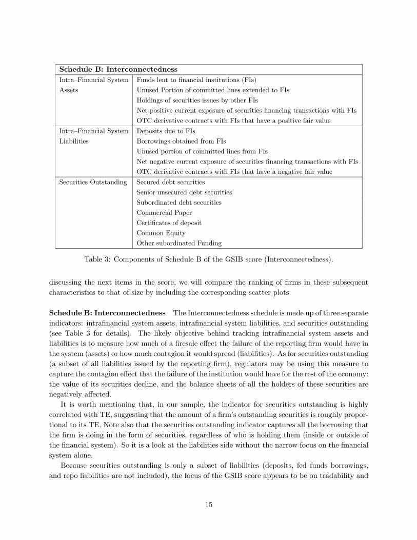
Schedule B: Interconnectedness

Intra—Financial System Funds lent to financial institutions (FIs)

Assets Unused Portion of committed lines extended to FIs

Holdings of securities issues by other FIs

Net positive current exposure of securities financing transactions with FIs

OTC derivative contracts with FIs that have a positive fair value

Intra—Financial System Deposits due to FIs

Liabilities Borrowings obtained from FIs

Unused portion of committed lines from FIs

Net negative current exposure of securities financing transactions with FIs

OTC derivative contracts with FIs that have a negative fair value

Securities Outstanding Secured debt securities

Senior unsecured debt securities

Subordinated debt securities

Commercial Paper

Certificates of deposit

Common Equity

Other subordinated Funding

Table 3: Components of Schedule B of the GSIB score (Interconnectedness).

discussing the next items in the score, we will compare the ranking of firms in these subsequent

characteristics to that of size by including the corresponding scatter plots.

Schedule B: Interconnectedness The Interconnectedness schedule is made up of three separate

indicators: intrafinancial system assets, intrafinancial system liabilities, and securities outstanding

(see Table 3 for details). The likely objective behind tracking intrafinancial system assets and

liabilities is to measure how much of a firesale effect the failure of the reporting firm would have in

the system (assets) or how much contagion it would spread (liabilities). As for securities outstanding

(a subset of all liabilities issued by the reporting firm), regulators may be using this measure to

capture the contagion effect that the failure of the institution would have for the rest of the economy:

the value of its securities decline, and the balance sheets of all the holders of these securities are

negatively affected.

It is worth mentioning that, in our sample, the indicator for securities outstanding is highly

correlated with TE, suggesting that the amount of a firm’s outstanding securities is roughly propor-

tional to its TE. Note also that the securities outstanding indicator captures all the borrowing that

the firm is doing in the form of securities, regardless of who is holding them (inside or outside of

the financial system). So it is a look at the liabilities side without the narrow focus on the financial

system alone.

Because securities outstanding is only a subset of liabilities (deposits, fed funds borrowings,

and repo liabilities are not included), the focus of the GSIB score appears to be on tradability and

15

1000 1500 2000 2500 3000 3500

Bank Size, $Billions

150

200

250

300

350

400

450

Inte

rcon

nect

edne

ss, $

Bill

ions

Interconnectedness, 6 Largest Banks

JPM

BoA

Citi

WF

GS

MS

50 100 150 200 250 300 350 400 450 500 550

Bank Size, $Billions

0

20

40

60

80

100

120

140

Inte

rcon

nect

edne

ss, $

Bill

ions

Interconnectedness, All but Top 6

S BCorp HSBC

PNC

BoNY

Cap. One

TD

State St.

BB&T Suntrust

Amex

C. Schwab Fifth

Ally

Citizens Regions

BMO Santander MUFG M&T

N. Trust

KeyCorp

Discover

Bancwest BBVA Comerica Huntigton Zions

DB

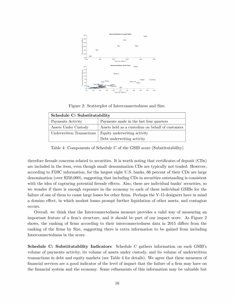
Figure 2: Scatterplot of Interconnectedness and Size.

Schedule C: Substitutability

Payments Activity Payments made in the last four quarters

Assets Under Custody Assets held as a custodian on behalf of customers

Underwritten Transactions Equity underwriting activity

Debt underwriting activity

Table 4: Components of Schedule C of the GSIB score (Substitutability)

therefore firesale concerns related to securities. It is worth noting that certificates of deposit (CDs)

are included in the item, even though small—denomination CDs are typically not traded. However,

according to FDIC information, for the largest eight U.S. banks, 66 percent of their CDs are large

denomination (over $250,000), suggesting that including CDs in securities outstanding is consistent

with the idea of capturing potential firesale effects. Also, these are individual banks’ securities, so

we wonder if there is enough exposure in the economy to each of these individual GSIBs for the

failure of one of them to cause large losses for other firms. Perhaps the Y-15 designers have in mind

a domino effect, in which modest losses prompt further liquidation of other assets, and contagion

occurs.

Overall, we think that the Interconnectedness measure provides a valid way of measuring an

important feature of a firm’s structure, and it should be part of our impact score. As Figure 2

shows, the ranking of firms according to their interconnectedness data in 2015 differs from the

ranking of the firms by Size, suggesting there is extra information to be gained from including

Interconnectedness in the score.

Schedule C: Substitutability Indicators Schedule C gathers information on each GSIB’s

volume of payments activity, its volume of assets under custody, and its volume of underwritten

transactions in debt and equity markets (see Table 4 for details). We agree that these measures of

financial services are a good indicator of the level of impact that the failure of a firm may have on

the financial system and the economy. Some refinements of this information may be valuable but

16

1000 1500 2000 2500 3000 3500

Bank Size, $Billions

0

2

4

6

8

10

12

Sub

stitu

tabi

lity,

$B

illio

ns

104 Substitutability, 6 Largest Banks

JPM

BoA

Citi

WF GS MS

50 100 150 200 250 300 350 400 450 500 550

Bank Size, $Billions

0

2

4

6

8

Sub

stitu

tabi

lity,

$B

illio

ns

104 Substitutability, All but Top 6

S BCorp HSBC PNC

BoNY

Cap. One TD

State St.

BB&T Suntrust Amex C. Schwab Fifth Ally Citizens Regions BMO Santander MUFG M&T

N. Trust

KeyCorp Discover Bancwest BBVA Comerica Huntigton Zions

DB

Figure 3: Scatterplot of Substitutability and Size.

may be difficult to implement.

One refinement would be to include information that helps regulators evaluate firms that are

important in these three categories also in terms of the risk they take in their business model.21

For example, a tri—party broker could choose two different business models: in one, it would simply

be a broker that performs custodian activities and derives its income mainly from service fees; in

another model, it would exploit its client relationships to also engage in providing intraday credit

to its clients, earning interest on such loans. We expect that loss given default would be much

higher in the second scenario.

Another refinement could be to capture information on the credit services that are associated

with underwriting of debt and equity issuance. It seems relevant to evaluate potential impact by

recognizing whether these “dealers” or “brokers” are also often the default buyers of the equity or

debt that they underwrite. As the importance of credit provision increases, loss given default is

amplified.

We recognize, however, the difficulties of measuring risk—taking and these two forms of credit

provision.22 Hence, overall, we think the characteristics captured in this schedule are relevant as

they are measured and should be part of our impact score. Figure 3 presents the scatterplot of

Substitutability and Size in 2015 for the Y-15 filers. It shows clearly that the ranking of firms

according to their substitutability data differs from the ranking of the firms by Size. In particular,

firms like State Street and BoNY, both of which have relatively small TEs but are responsible for a

significant fraction of the provision of custodian services (high payments and assets under custody

scores), are clearly outliers in the scatterplot. This suggests there is extra information to be gained

from including substitutability in the score.

Schedule D: Complexity Indicators There are three components in the complexity score:

OTC derivatives, trading and available for sale (AFS) securities, and level 3 assets (see Table 5 for

21For an argument along these lines, see Duffie (2014).22See Begenau, Piazzesi and Schneider (2015) for a study of risk—taking by the main broker-dealers in the U.S.

17

Schedule D: Complexity

Notional OTC Derivatives OTC derivative contracts cleared through central counterparty

OTC derivative contracts settled bilaterally

Trading and AFS Securities Trading securities

Available—for—sale (AFS) securities

Level 3 Assets Assets valued for accounting purposes using Level 3 measurement inputs

Table 5: Components of Schedule D of the GSIB score (Complexity).

Trading Available—for—Sale (AFS) Held to maturity

Selling restrictions Expected to be sold Meant to be held longer Meant to be held to

within, approximately, than a year but expected maturity, not sold

one year to besold before they

reach maturity

Accounting valuation Fair value Fair value Book value

method

Accounting of Recorded in the income Do not affect earnings and are Not reported

unrealized changes in statement as earnings only recorded in a separate

value form (shareholders’ value)

until they are realized

Table 6: Classification of securities

details). We discuss each of those in turn.

OTC derivatives OTC Derivatives are bilateral contracts (even if cleared through a CCP),

and hence they may be used to hedge trades and risks specific to the firm’s counterparty. They

likely are counted toward loss given default in the GSIB score, because, if the institution fails, its

counterparty in these derivatives may have difficulty finding a new counterparty that desires an

equivalent position.

Trading and available—for—sale securities Securities are classified, at the time of purchase,

into one of the following three categories for accounting purposes: trading, available—for—sale (AFS),

and held—to—maturity. Mark—to—market changes in the valuation of trading securities and AFS

securities have different consequences for income: changes in the value of trading securities appear

as expenses/income in the income statement, while changes in the value of AFS securities affect

only equity. Changes in the value of held—to—maturity securities do not affect either income or

equity. Table 6 summarizes the differences.

Note that classification occurs at the time of purchase and can only be changed at the next

reporting period. Moreover, FASB guidance states that only reclassifications from AFS to held—to—

maturity are viewed as normal. Other reclassifications require special reporting and justification

(acceptable reasons for the reclassification of held—to—maturity include, for example, the risk of a

18

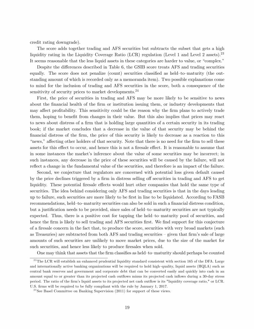
credit rating downgrade).

The score adds together trading and AFS securities but subtracts the subset that gets a high

liquidity rating in the Liquidity Coverage Ratio (LCR) regulation (Level 1 and Level 2 assets).23

It seems reasonable that the less liquid assets in these categories are harder to value, or “complex.”

Despite the differences described in Table 6, the GSIB score treats AFS and trading securities

equally. The score does not penalize (count) securities classified as held—to—maturity (the out-

standing amount of which is recorded only as a memoranda item). Two possible explanations come

to mind for the inclusion of trading and AFS securities in the score, both a consequence of the

sensitivity of security prices to market developments.24

First, the price of securities in trading and AFS may be more likely to be sensitive to news

about the financial health of the firm or institution issuing them, or industry developments that

may affect profitability. This sensitivity could be the reason why the firm plans to actively trade

them, hoping to benefit from changes in their value. But this also implies that prices may react

to news about distress of a firm that is holding large quantities of a certain security in its trading

book; if the market concludes that a decrease in the value of that security may be behind the

financial distress of the firm, the price of this security is likely to decrease as a reaction to this

“news,” affecting other holders of that security. Note that there is no need for the firm to sell these

assets for this effect to occur, and hence this is not a firesale effect. It is reasonable to assume that

in some instances the market’s inference about the value of some securities may be incorrect; in

such instances, any decrease in the price of these securities will be caused by the failure, will not

reflect a change in the fundamental value of the securities, and therefore is an impact of the failure.

Second, we conjecture that regulators are concerned with potential loss given default caused

by the price declines triggered by a firm in distress selling off securities in trading and AFS to get

liquidity. These potential firesale effects would hurt other companies that hold the same type of

securities. The idea behind considering only AFS and trading securities is that in the days leading

up to failure, such securities are more likely to be first in line to be liquidated. According to FASB

recommendations, held—to—maturity securities can also be sold in such a financial distress condition,

but a justification needs to be provided, since sales of held—to—maturity securities are not typically

expected. Thus, there is a positive cost for tapping the held—to—maturity pool of securities, and

hence the firm is likely to sell trading and AFS securities first. We find support for this conjecture

of a firesale concern in the fact that, to produce the score, securities with very broad markets (such

as Treasuries) are subtracted from both AFS and trading securities — given that firm’s sale of large

amounts of such securities are unlikely to move market prices, due to the size of the market for

such securities, and hence less likely to produce firesales when sold.

One may think that assets that the firm classifies as held—to—maturity should perhaps be counted

23The LCR will establish an enhanced prudential liquidity standard consistent with section 165 of the DFA. Large

and internationally active banking organizations will be required to hold high—quality, liquid assets (HQLA) such as

central bank reserves and government and corporate debt that can be converted easily and quickly into cash in an

amount equal to or greater than its projected cash outflows minus its projected cash inflows during a 30-day stress

period. The ratio of the firm’s liquid assets to its projected net cash outflow is its "liquidity coverage ratio," or LCR.

U.S. firms will be required to be fully compliant with the rule by January 1, 2017.24See Basel Committee on Banking Supervision (2011) for support of these views.

19

in the impact score given that their value could be more opaque (since they are accounted at book

value and traded less often). As it turns out, this is already taken care of by the “Level 3 assets”

item in the score, which we discuss next.

Level 3 assets25 “Level 3” is an accounting classification for assets that are deemed complex

to evaluate (because there is no clear market price or a standard valuation model). The score

likely penalizes them because complexity implies less value in bankruptcy, or in a rushed sale

when attempting to avoid bankruptcy, and hence implies more losses to debt holders. Because the

discount that these assets would suffer in a rushed sale is due to complexity, and not due to a large

quantity of them being sold in the market, we do not consider this a firesale effect.

The FASB rule specifying which types of assets are classified as Level 3 (FAS 157) has a some-

what tenuous classification criterion: those measured “using significant unobservable inputs.”26 For

example, if a market price is available, the asset is considered Level 1; if an option can be priced

using the Black—Scholes model, that option is considered a Level 2 item, because a model is used

but data on volatility can be gathered from past behavior of prices. In contrast, the valuation

of the stock of a private company requires making assumptions about the future profitability of

that company — needing what accountants call “assumptions about market assumptions”: what

the company thinks the market will use as the valuation for an asset, etc., so is classified as a Level

3 item.

Note that the score attempts to gather information that is comparable (or harmonized) interna-

tionally; hence, rather than choosing a list of specific asset classes that regulators view as complex,

they pick an international classification of assets (Level 3) that is typically applied to complex

assets.

Overall, we find that schedule D accounts for important firm characteristics and that all of its

items should be included in our impact score. As Figure 4 shows, the ranking of firms according

to their complexity data in 2015 differs from the ranking of the firms by Size, suggesting there is

extra information to be gained from including complexity in the score.

Schedule E: Cross—Jurisdictional Activity Indicators As Table 7 indicates, this schedule

essentially collects just two figures: 1) The sum of all amounts owed — including positive values of

derivatives — to the filing bank by foreign persons, public institutions, financial firms, and nonfinan-

cial firms; and 2) the sum of all amounts owed by the filing bank to foreigners (including amounts

owed by the filer’s foreign offices – amounts owed in both local and nonlocal currencies of these

offices).27 The idea here is that assets and liabilities that cross national borders are more complex

to collect if the borrower becomes troubled, because of differences in bankruptcy treatment across

countries and the chance that assets might be ring—fenced. We think this is a valid concern, and

25Note that Level 1,2,3 in FASB is different than Level 1 and 2 liquid assets in the previous point (that classification

is instead derived from the LCR calculation in 12 CFR 249.20(a)).26See Financial Accounting Standards Board, “Original Pronouncements, As Amended, State-

ment of Financial Accounting Standards No. 157, Fair Value Measurements.” P. 29, available at:

http://www.fasb.org/jsp/FASB/Document_C/DocumentPage?cid=1218220130001&acceptedDisclaimer=true.27For U.S. Y-15 filers, these data are reported on FFIEC Form 009 and the Treasury International Capital reports.

20

1000 1500 2000 2500 3000 3500

Bank Size, $Billions

0

0.5

1

1.5

2

Com

plex

ity, $

Bill

ions

104 Complexity, 6 Largest Banks

JPM

BoA Citi

WF

GS

MS

50 100 150 200 250 300 350 400 450 500 550

Bank Size, $Billions

0

500

1000

1500

2000

2500

Com

plex

ity, $

Bill

ions

Complexity, All but Top 6

S BCorp

HSBC

PNC

BoNY

Cap. One TD

State St.

BB&T Suntrust Amex C. Schwab Fifth Ally Citizens Regions BMO Santander MUFG M&T N. Trust

KeyCorp Discover Bancwest BBVA Comerica Huntigton Zions DB

Figure 4: Scatterplot of Complexity and Size.

1000 1500 2000 2500 3000 3500

Bank Size, $Billions

100

200

300

400

500

600

700

800

Cro

ss J

uris

dict

iona

l Act

ivity

, $B

illio

ns

Cross Jurisdictional Activity, 6 Largest Banks

JPM

BoA

Citi

WF

GS MS

50 100 150 200 250 300 350 400 450 500 550

Bank Size, $Billions

0

50

100

150

Cro

ss J

uris

dict

iona

l Act

ivity

, $B

illio

ns

Cross Jurisdictional Activity, All but Top 6

S BCorp HSBC

PNC

BoNY

Cap. One TD

State St.

BB&T Suntrust

Amex

C. Schwab Fifth Ally Citizens Regions BMO Santander MUFG M&T

N. Trust

KeyCorp Discover Bancwest BBVA Comerica Huntigton Zions DB

Figure 5: Scatterplot of Cross—Jurisdictional Activity and Size

that the items in this schedule should be part of our impact score. As Figure 5 shows, the ranking

of firms according to their cross—jurisdictional activity data in 2015 differs from the ranking of the

firms by Size, suggesting there is extra information to be gained from including this characteristic

in the score.

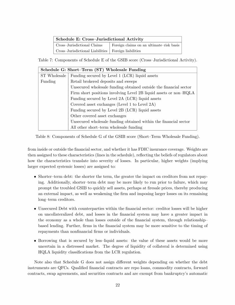
Schedule G: Proportion of risk—weighted assets that are funded through short—term

debt This schedule is an attempt to quantify the potential losses to the economy that might arise

when a GSIB firm is a heavy user of certain types of short—term funding. Details on the information

collected are in Table 8. Use of short—term debt is measured as a percentage of risk—weighted assets.

GSIBs only began completing Schedule G in December 2016, and data will not be released until

November 2017, so as of this writing, the currently available GSIB scores do not incorporate data

from this new schedule.

The schedule collects information on how the debt of the firm is distributed across different

characteristics including remaining maturity, liquidity of collateral, whether the debt is obtained

21

Schedule E: Cross—Jurisdictional Activity

Cross—Jurisdictional Claims Foreign claims on an ultimate—risk basis

Cross—Jurisdictional Liabilities Foreign liabilities

Table 7: Components of Schedule E of the GSIB score (Cross—Jurisdictional Activity).

Schedule G: Short—Term (ST) Wholesale Funding

ST Wholesale Funding secured by Level 1 (LCR) liquid assets

Funding Retail brokered deposits and sweeps

Unsecured wholesale funding obtained outside the financial sector

Firm short positions involving Level 2B liquid assets or non—HQLA

Funding secured by Level 2A (LCR) liquid assets

Covered asset exchanges (Level 1 to Level 2A)

Funding secured by Level 2B (LCR) liquid assets

Other covered asset exchanges

Unsecured wholesale funding obtained within the financial sector

All other short—term wholesale funding

Table 8: Components of Schedule G of the GSIB score (Short—Term Wholesale Funding).

from inside or outside the financial sector, and whether it has FDIC insurance coverage. Weights are

then assigned to these characteristics (lines in the schedule), reflecting the beliefs of regulators about

how the characteristics translate into severity of losses. In particular, higher weights (implying

larger expected systemic losses) are assigned to:

• Shorter—term debt: the shorter the term, the greater the impact on creditors from not repay-

ing. Additionally, shorter—term debt may be more likely to run prior to failure, which may

prompt the troubled GSIB to quickly sell assets, perhaps at firesale prices, thereby producing

an external impact, as well as weakening the firm and imposing larger losses on its remaining

long—term creditors.

• Unsecured Debt with counterparties within the financial sector: creditor losses will be higheron uncollateralized debt, and losses in the financial system may have a greater impact in

the economy as a whole than losses outside of the financial system, through relationship—

based lending. Further, firms in the financial system may be more sensitive to the timing of

repayments than nonfinancial firms or individuals.

• Borrowing that is secured by less—liquid assets: the value of these assets would be moreuncertain in a distressed market. The degree of liquidity of collateral is determined using

HQLA liquidity classifications from the LCR regulation.

Note also that Schedule G does not assign different weights depending on whether the debt

instruments are QFCs. Qualified financial contracts are repo loans, commodity contracts, forward

contracts, swap agreements, and securities contracts and are exempt from bankruptcy’s automatic

22

stay. A key component of bankruptcy, the automatic stay prevents, upon a debtor’s bankruptcy

filing, most creditors from attempting to collect on their claims. The primary objective of the stay

is to avoid the separation of complementary assets and to preserve the going—concern value of a

firm. QFCs, however, are exempt from the automatic stay so that investors who hold them have

the ability to immediately take possession (and sell, if they wish) any collateral that backs their

loans or derivatives. This is beneficial because it avoids contagion to counterparties. QFCs are,

hence, mostly used by counterparties who are particularly sensitive to the timing of repayments,

and would be particularly hurt by an automatic stay.28 As we have mentioned, a potential cost

of the exemption from the stay is the separation of complementary assets. However, the collateral

backing QFCs is typically not complementary to other assets of the firm, nor will QFC collateral be

important to the firm’s going—concern value. For example, QFC collateral often consists of highly

marketable or cash—like securities (for example Treasury debt instruments), which can be removed

from the firm without reducing the value of other firm assets. Broadly, therefore, QFCs are exempt

from bankruptcy’s stay because they are considered especially “systemic” instruments while, at the

same time, the collateral that backs QFCs consists mainly of assets that can be removed from the

failing firm without producing a large impact on the failing firm’s liquidation value.

The fact that Schedule G does not assign special weight to QFCs seems to implicitly assume

that there might be losses imposed on creditors even if they are lending to GSIBs through QFCs.

Perhaps the designers of the GSIB score considered the possibility that, while QFC—based lending

allows creditors to protect themselves by quickly seizing collateral in bankruptcy, creditors still

may suffer losses if they sell the seized collateral en masse, producing firesale losses. If that is the

case, losses might also extend beyond the creditors of a bankrupt GSIB to other holders of similar

assets.

Overall, we think that it is important for any impact score to include information about a firm’s

short—term debt structure. However, we have some suggestions on ways to capture this structure

in a way that may be more informative about the failure’s impact. Mainly, the weighted short—

term debt instruments are normalized in the GSIB score by dividing by risk—weighted assets, with

only the normalized ratio entering the GSIB score calculation. But because risk—weighted assets

generally discount assets like Treasuries, which are very liquid and hence less likely to imply losses

if they need to be liquidated to meet short—term debt obligations, we believe it would be more

appropriate to simply use assets as the denominator for the Schedule G indicator. In other words,

using risk—weighted assets to normalize may inappropriately penalize those GSIBs that have large

holdings of very liquid assets. In fact, a high proportion of short—term funding is less troublesome

if the GSIB matches this funding with an equivalent portion of liquid assets. As a result, a measure

that compares short—term debt with liquid assets (such as the one that the LCR rule requires),

which we propose to use (see next section), would be even more informative about the impact of

short—term debt use in a firm’s resolvability.

Moreover, we propose that the total amount of QFCs and of non—QFC short—term debt be

recorded and evaluated separately. In the next section, we discuss this idea and propose specific

28See Pellerin and Walter (2012) for a discussion of the idea that QFCs are in a special class of financial instruments

(p. 20) and of the role of QFCs in resolution (p. 19-24).

23

New items: structure of short—term (ST) debt

QFCs Fed funds and repo borrowing

Derivatives purchased with negative fair value

Derivatives sold with negative fair value

QFCs/ Assets QFCs (as defined above) over total assets

Non—QFC ST debt Commercial paper

Other borrowed money with remaining maturity of one year or less

Uninsured deposits

Non—QFC ST debt / Assets Our measure of non—QFC ST debt above, over total assets

1/LCR Our measure of non—QFC ST debt plus Fed funds and repo borrowing,

all divided by the amount of high quality liquid assets

Table 9: New items in the impact score.

ways to measure the impact of the short—term debt structure of firms.

4 New items for the score

In this section, we discuss some firm characteristics that we view as valuable additions our impact

score, above and beyond what the GSIB score considers. Because the Y-15 does not collect these

items, we assemble them from other regulatory filings, specifically from financial statements for

bank holding companies (FR Y-9C) and financial statements for banks (“Call Reports” — FFIEC

031). Table 9 lists these new items, which all relate to the structure of a firm’s short—term debt.

The appendix contains the details on how we construct each of them.

The amount and structure of short—term funding is important for resolution because these

features determine, to an important extent, post—failure outcomes: the DIP financing needs of the

firm; the potential for firesales; and possible losses to creditors. Importantly, differing resolution

methods (bankruptcy, OLA, or bailout) will likely influence these outcomes because the resolution

method chosen may result in different treatment of debtors. In order for our score to address these

important differences, in what follows we split the main impact of the structure of short—term debt

into (i) inability to perform financial functions essential to the economy because of the lack of DIP

financing, (ii) firesale effects, and (iii) contagion effects. We propose measurable firm characteristics

to be added as items in the score and discuss why each of them would be informative about each

of the three effects.

Inability to perform financial functions essential to the economy because of a post—

failure lack of sufficient DIP financing

We expect the amount of short—term debt to be an indicator of DIP financing requirements

post—failure: if we assume all short—term creditors pull out prior to failure, the firm will require

DIP financing to replace this funding following failure and allow the firm to continue its former

activities.29 The larger the quantity of DIP financing required, the more challenging will be the job

29 It is difficult to anticipate how much of a troubled firm’s short-term financing will remain at the time failure is

24

1000 1500 2000 2500 3000 3500

Bank Size, $Billions

0

0.2

0.4

0.6

0.8

1

QFC

Deb

t to

Asse

ts, P

erce

nt

QFC Debt to Assets, 6 Largest Banks

JPM BoA

Citi

WF

GS

MS

0 100 200 300 400 500 600

Bank Size, $Billions

0

0.1

0.2

0.3

0.4

0.5

0.6

QFC

Deb

t to

Asse

ts, P

erce

nt

QFC Debt to Assets, All but Top 6

S BCorp

HSBC

PNC

BoNY

Cap. One TD

State St.

BB&T Suntrust

Amex C. Schwab Fifth Ally Citizens Regions

BMO Santander MUFG M&T N. Trust KeyCorp Discover Bancwest BBVA Comerica Huntigton Zions

DB

1000 1500 2000 2500 3000 3500

Bank Size, $Billions

0

200

400

600

800

1000

1200

QFC

Deb

t, $B

illion

s

QFC Debt, 6 Largest Banks

JPM

BoA

Citi

WF

GS

MS

0 100 200 300 400 500 600

Bank Size, $Billions

0

20

40

60

80

100

120

140Q

FC D

ebt,

$Billi

ons

QFC Debt, All but Top 6

S BCorp

HSBC

PNC

BoNY

Cap. One TD

State St.

BB&T Suntrust

Amex C. Schwab Fifth Ally Citizens Regions BMO Santander MUFG M&T N. Trust KeyCorp Discover Bancwest BBVA Comerica Huntigton Zions DB

Figure 6: Scatterplot of QFC financing (right), and its ration to assets (left), and size.

of finding a lender with sufficient capacity to provide the needed DIP loan. Lack of DIP funding

will make it more difficult for the firm to keep healthy subsidiaries working and performing financial

functions that may be essential to the economy. The firm characteristics that can be informative

about this effect are:

• QFC financing: These financing sources will disappear even if they do not run prior to failure,because they are exempt from bankruptcy’s automatic stay.

• Non—QFC short—term debt: These financing sources can run prior to failure, but not after,

so assuming all of this debt runs before failure provides an upper bound on impact.

Figure 6 presents the scatterplot of the ratio to assets (left) and the amount (right) of QFC

financing and size, while Figure 7 presents the non—QFC debt counterparts.

Contagion to creditors of the failing firm

There are two main types of debt holders: short—term creditors and long—term creditors. Be-

cause their treatment in a failure may differ according to the resolution method, we discuss the

informativeness of short—term debt structure about contagion to each of these two classes of credi-

tors separately.

declared because creditors often detect the firm’s problems and withdraw funding in the days leading up to a failure.

In our analysis, we consider both extreme scenarios (prior to failure either all debt runs or, alternatively, none of it

runs) in order for our score to capture the largest impact a failure might produce.

25

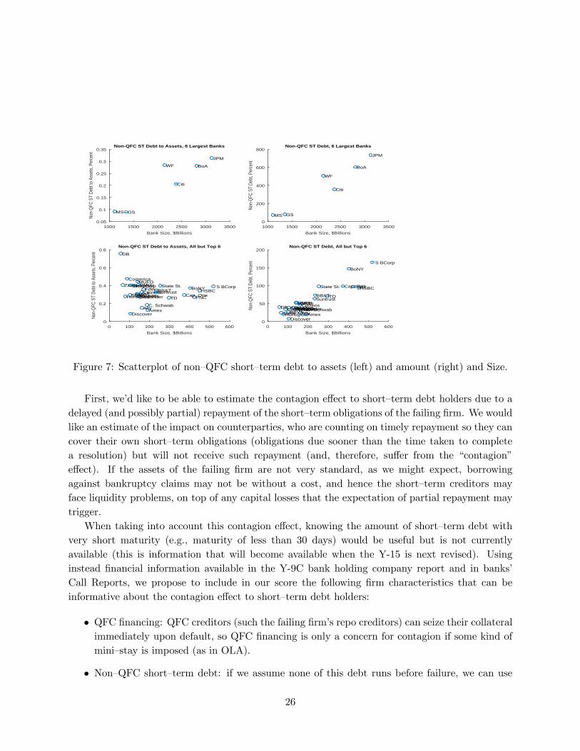
1000 1500 2000 2500 3000 3500

Bank Size, $Billions

0.05

0.1

0.15

0.2

0.25

0.3

0.35

Non-

QFC

ST

Debt

to A

sset

s, P

erce

nt

Non-QFC ST Debt to Assets, 6 Largest Banks

JPM

BoA

Citi

WF

GS MS

0 100 200 300 400 500 600

Bank Size, $Billions

0

0.2

0.4

0.6

0.8

Non-

QFC

ST

Debt

to A

sset

s, P

erce

nt

Non-QFC ST Debt to Assets, All but Top 6

S BCorp HSBC

PNC

BoNY

Cap. One TD

State St. BB&T Suntrust

Amex C. Schwab

Fifth

Ally

Citizens Regions

BMO

Santander

MUFG

M&T N. Trust

KeyCorp

Discover

Bancwest

BBVA

Comerica

Huntigton

Zions

DB

1000 1500 2000 2500 3000 3500

Bank Size, $Billions

0

200

400

600

800

Non-

QFC

ST

Debt

, Per

cent

Non-QFC ST Debt, 6 Largest Banks

JPM

BoA

Citi

WF

GS MS

0 100 200 300 400 500 600

Bank Size, $Billions

0

50

100

150

200No

n-Q

FC S

T De

bt, P

erce

ntNon-QFC ST Debt, All but Top 6

S BCorp

HSBC PNC

BoNY

Cap. One

TD

State St.

BB&T Suntrust

Amex C. Schwab

Fifth

Ally

Citizens Regions BMO Santander MUFG M&T N. Trust KeyCorp

Discover

Bancwest BBVA

Comerica Huntigton Zions

DB

Figure 7: Scatterplot of non—QFC short—term debt to assets (left) and amount (right) and Size.

First, we’d like to be able to estimate the contagion effect to short—term debt holders due to a

delayed (and possibly partial) repayment of the short—term obligations of the failing firm. We would

like an estimate of the impact on counterparties, who are counting on timely repayment so they can

cover their own short—term obligations (obligations due sooner than the time taken to complete

a resolution) but will not receive such repayment (and, therefore, suffer from the “contagion”

effect). If the assets of the failing firm are not very standard, as we might expect, borrowing

against bankruptcy claims may not be without a cost, and hence the short—term creditors may

face liquidity problems, on top of any capital losses that the expectation of partial repayment may

trigger.

When taking into account this contagion effect, knowing the amount of short—term debt with

very short maturity (e.g., maturity of less than 30 days) would be useful but is not currently

available (this is information that will become available when the Y-15 is next revised). Using

instead financial information available in the Y-9C bank holding company report and in banks’

Call Reports, we propose to include in our score the following firm characteristics that can be

informative about the contagion effect to short—term debt holders:

• QFC financing: QFC creditors (such the failing firm’s repo creditors) can seize their collateralimmediately upon default, so QFC financing is only a concern for contagion if some kind of

mini—stay is imposed (as in OLA).

• Non—QFC short—term debt: if we assume none of this debt runs before failure, we can use

26

this amount as an upper bound on this impact.

Second, we would like to estimate potential losses to long—term debt holders (and any short—

term creditors who do not run) from the liquidation of assets to repay short—term debt that has

run. For this objective, we need information about the relative importance of losses for the firm

stemming from the rushed liquidation of those assets; this will be informative about the decrease

in the value of total assets that the run of the short—term debt will impose and hence on the losses

imposed on long—term debt holders by decreasing the value of the firm’s assets in bankruptcy.

Note, as discussed below, that some policymakers may be more concerned with this firesale effect

than others — in other words, some policymakers may believe it unlikely that asset values can be

driven below fundamental values. Using financial information from the Y-9C and Call Reports, we

propose to include in our score the following firm characteristics that can be informative about this

contagion effect to long—term debt holders:

• Ratio of QFC financing to assets: for these debt instruments, typically, there will be marginson derivatives, or haircuts on repo collateral, to compensate counterparties for the risk of

default on the contract. Such instruments imply losses for the failed firm when its QFC

contracts are terminated, which translates into lower recovery rates for the failed firm’s non—

QFC creditors.

• Non—QFC short—term debt to assets ratio: similar to the case of QFCs, but here losses, if any,would come from a firesale effect, where the liquidation of assets to cover running non—QFC

debt can drive the value of these assets below their fundamental values. If we assume all

short—term debt runs, this provides an upper bound for this impact.

• Inverse of LCR: the proportion of highly liquid assets to short—term debt (inverse of the LCR)provides a measure of expected losses that might be suffered by long—term debt holders from

the rushed liquidation of assets to repay short—term obligations that are removed prior to

failure: a firm that relies heavily on short—term debt but has very liquid assets may avoid

large losses in the days leading up to failure, while one that has to sell illiquid assets is likely

to suffer losses on such sales. A higher ratio will mean lower losses on the proportion of the

balance sheet that is financed by short—term debt.

Figure 8 presents the scatterplot of the inverse of the LCR (short—term debt over assets) and

size.

Contagion to third parties through a balance—sheet effect of firesales of assets

If creditors become unwilling to roll over the troubled firm’s short—term debt in the weeks or

days leading up to the failure of a firm, the amount of a firm’s short—term financing will be an

ex—ante indicator of potential firesale effects: the larger the amount of short—term debt, the larger

the amount of assets that will have to be liquidated by the troubled firm (to repay creditors that

are unwilling to roll over) to try to maintain the firm’s solvency, and the greater the potential for

firesales. The firm characteristics that can be informative about this effect are:

27

1000 1500 2000 2500 3000 3500

Bank Size, $Billions

1.2

1.4

1.6

1.8

2

ST

Deb

t HQ

LA r

atio

, Rat

io

ST Debt HQLA ratio, 6 Largest Banks

JPM

BoA

Citi WF

GS

MS

50 100 150 200 250 300 350 400 450 500 550

Bank Size, $Billions

0.5

1

1.5

2

2.5

3

3.5

4

ST

Deb

t HQ

LA r

atio

, Rat

io

ST Debt HQLA ratio, All but Top 6

S BCorp

HSBC

PNC

BoNY

Cap. One

TD

State St.

BB&T Suntrust

Amex

C. Schwab

Fifth

Ally

Citizens

Regions

BMO

Santander

MUFG

M&T

N. Trust

KeyCorp

Discover

Bancwest BBVA

Comerica Huntigton

Zions

DB

Figure 8: Scatterplot of the inverse of the LCR ratio (short—term debt over assets) and Size.

• QFC financing: because these instruments are exempt from the automatic stay, even if QFC—based funding doesn’t run prior to failure, this funding will be liquidated upon failure. As a

result of this liquidation, the collateral may land in the hands of a counterparty which values

the collateral less than the failed firm. Alternatively, the collateral may go to a creditor that

does not want to hold it, leading to the sale of a large quantity of the collateral. Either may

depress the asset’s market price.

• Non—QFC short—term debt: any of this type of debt may also have a firesale effect if it runs

before the automatic stay is declared. Hence, assuming all of it runs we can use this amount

as an upper bound on this effect.

As the discussion in this section makes clear, there are different possible costs and benefits to

a GSIB firm’s heavy use of QFCs, and the sum of the costs and benefits, should the firm fail, is

unclear for the financial system or the economy as a whole. Further, as we will discuss in more

detail below, different policymakers may weight each of these costs and benefits differently.

4.1 A snapshot of large U.S. firms using our new impact—relevant characteristics

Figure 9 presents the raw data on both the GSIB original firm characteristics and the new charac-

teristics we have proposed as relevant to calculate impact, for the 34 BHCs in 2015. We use a color

scheme to illustrate the relative importance of each number (red corresponds to larger numbers,

yellow to intermediate, and green to smaller). Firms are ordered according to their size (as mea-

sured by Total Exposures), from largest to smallest. This allows us to compare all characteristics at

the same time, as opposed to one by one, to size, as we did in the scatterplot figures above. Green

28

colors in the top rows, or red colors on the bottom rows, indicate deviations from a proportional

relationship of the characteristic being measured and size. For example, Bank of New York Mellon

and State Street both score very high on substitutability given their size, because of their roles

as intermediaries in the Tri—party repo market (they have a disproportionately high number of

assets under custody). As another example, Wells Fargo scores relatively low in Substitutability,

Complexity and Cross—Jurisdictional activity, given that it is the 4th largest bank.

It is worth discussing the facts regarding some of our new items. QFC amount is fairly propor-

tional to size, but this is less true for QFC/Assets. More importantly, even though the amount of

non—QFC short—term debt is proportional to size, the ratio of this type of debt to assets displays

an almost inverse relationship to size. This inverse relationship is also somewhat present in our

approximation of the inverse of the LCR, with many large firms showing a high proportion of liq-

uid assets to short term debt, and instead many smaller firms showing high levels of illiquidity as

measured by our ratio.

Differences in these characteristics of the debt structure may translate into important differences

in impact following failure, as we have discussed. In the next section we will illustrate how differ-

ences of opinion regarding the mapping of these characteristics into impact may affect judgement

calls on whether firms have an acceptable structure for resolution through bankruptcy.

5 Evaluating acceptable firm structures

We have discussed how a modified version of the existing GSIB score could be a good candidate for

a measure meant to establish whether a firm’s structure is acceptable for resolution in bankruptcy

– an impact score. We now illustrate how to use weights in the score to account for the fact that

the same objective quantity recorded for a given firm characteristic may translate into different

levels of impact depending on the resolution method used to deal with the troubled firm or on the

crisis scenario being considered. We will use the score in a positive way, as an instrument to portray

different opinions that hypothetical policymakers may have concerning the impact associated with

these characteristics. With this exercise we want to emphasize that these scores may be influenced

by subjective beliefs of policymakers.

In our examples, we use actual data on firm characteristics (collected by the Y-15, plus estimates

of the importance of short—term funding and of the use of QFCs that we calculate using publicly

available data from the Y-9C and the Call Report). We combine these data with three different

sets of weights (see Figure 10), which we created in order to represent views of three “types”

of policymakers. The combination of actual firm data with weights that we devised produces

hypothetical scores that we use to study these hypothetical policymakers’ views about various

firms’ resolvability.30

In the next paragraphs we discuss, for several indicators, reasons that could be behind any

difference of opinion on how the impact of a given firm characteristic would differ across different

30An Excel spreadsheet to calculate our impact score is available as an online appendix. It allows readers to adjust

policymaker’s weights, based on their own views of the likely impacts associated with various firm characteristics,

scenarios, and resolution methods, and examine how such changes shift scores for the 33 institutions required to file

the Y-15 in 2015.

29

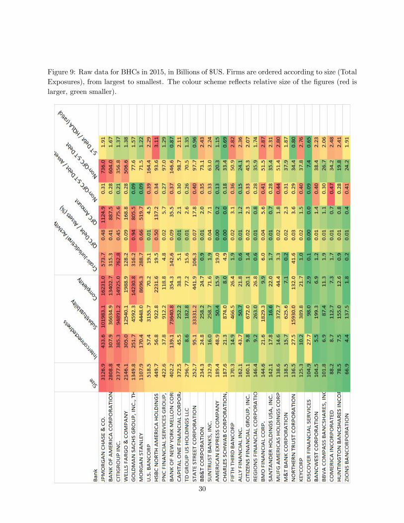
Figure 9: Raw data for BHCs in 2015, in Billions of $US. Firms are ordered according to size (Total

Exposures), from largest to smallest. The colour scheme reflects relative size of the figures (red is

larger, green smaller).

30

resolution methods and scenarios. We then use these different arguments to characterize the beliefs,

or weights, of our three hypothetical policymakers: we propose a ranking of the weights within each

characteristic and come up with numbers in our example (Figure 10) that will satisfy these rankings.

Policymaker 1 has two sets of weights, labeled (a) and (b), representing his views at two points

in time. The weights in (a) can be thought of as representing a Policymaker that currently agrees

with LW reviewers at the Federal Reserve and the FDIC, who have recently determined that all of

the large firms have acceptable LWs. As we will see when we present the results of our examples,

we set this first set of weights on firm characteristics such that, in fact, all the firms in our sample

have an acceptable structure. For contrast, the weights for Policymaker 1 in case (b), though

matching the relative importance of each characteristic with those in case (a), are twice as large

for each characteristic. This will imply, as we will see, that some of the firm’s structures are not

acceptable in a hypothetical case (a). With these two contrasting weights we want to capture:

1) some policymakers’ views that the TBTF problem has become less severe as a result of the

legislative and regulatory efforts in the last 10 years geared toward assuring less costly large firm

resolution; and 2) views that policymakers might have held before these changes were implemented.

In particular, we are focusing on the shifts that were driven by international regulations such

as Basel III and several important legislative and regulatory changes introduced since the finan-

cial crisis of 2007 — 2008. These legislative and regulatory changes include TLAC, new liquidity

standards, and implementation of the living will process. Because of these measures, we model

Policymaker 1’s beliefs as shifting from (b) (before the crisis) to (a) (currently). Current weights

represent the belief that the failure of a bank is likely to lead to considerably less economic impact

than would have occurred prior to these changes.

When modelling the shift in beliefs of Policymaker 1 from (a) to (b), we also adjust the estimates

for the cost of government intervention. As we discuss in detail in the next subsection, these costs

can include not only efficiency losses due to risk shifting (i.e., moral hazard costs) but also bailout

“outrage” costs. In particular, in case (b), before the big bailouts of 2008, these outrage costs

may have been lower than today (case (a)). Intense public protests and legislator criticism of

bailouts and other forms of government assistance, following the crisis, imply that policymakers

can anticipate similar opposition in response to any future bank bailout or assistance. Moreover,

it seems possible that the last decade’s regulatory efforts imply an increase in the moral hazard

consequences of a bailout: if, after all the costly LW process and other efforts, a firm gets bailed

out, other firms in the financial system and their creditors are likely to increase expectations of a

future bailout out.

Alternatively, we could interpret case (b) for Policymaker 1 as representing the views of a current

policymaker who is not convinced that legislative and regulatory shifts have yet been sufficient to

significantly reduce the economic impact of a large bank’s failure. Therefore, for this policymaker,

the TBTF problem has not been reduced.

To further illustrate how our “acceptability” determinations depend on weights, we propose

two more policymakers (2 and 3) who share Policymaker’s 1(b) estimates of the cost of government

intervention, but disagree with him in some of their weights. This choice of the cost of government

intervention for Policymakers 2 and 3 is purely out of convenience (we need variation in the resolv-

31

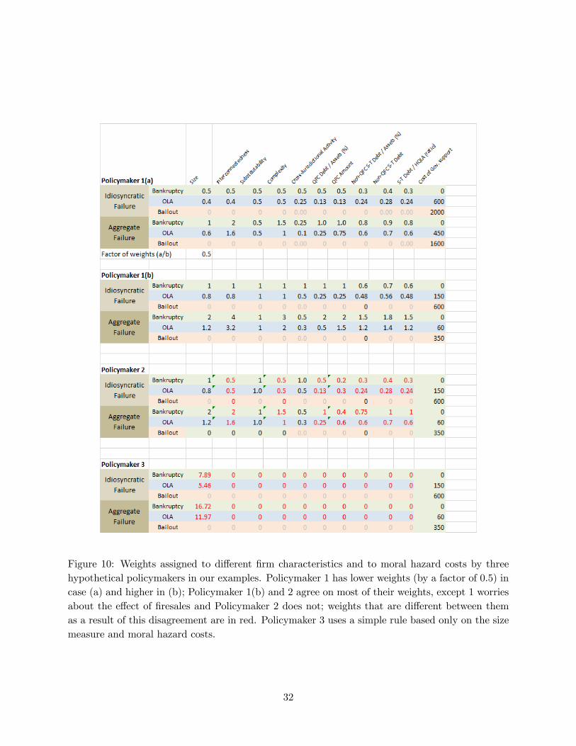
Figure 10: Weights assigned to different firm characteristics and to moral hazard costs by three

hypothetical policymakers in our examples. Policymaker 1 has lower weights (by a factor of 0.5) in

case (a) and higher in (b); Policymaker 1(b) and 2 agree on most of their weights, except 1 worries

about the effect of firesales and Policymaker 2 does not; weights that are different between them

as a result of this disagreement are in red. Policymaker 3 uses a simple rule based only on the size

measure and moral hazard costs.

32

ability determinations to illustrate how our score works), but in no sense do we mean to imply that

Policymaker 1’s weights in (b) are more realistic, or reasonable.

Policymaker 1 (a and b) worries about firesales. Policymaker 2, instead, does not believe that

the firesales are a significant concern. Hence, the weights on characteristics that may involve firesale

estimates will be typically higher for Policymaker 1 than for Policymaker 2 (the weights that differ

are indicated in red in Figure 10). One can think of Policymaker 1 as being broadly representative

of those policymakers who are very worried about external effects emanating from the failure of a

GSIB and Policymaker 2 as representative of those more skeptical about such effects.31

Policymaker 3 wants a simple score based only on size. He has the same weights as Policymaker

1, but he only analyzes the individual firm characteristics for the largest five holding companies.

Then, he chooses alternative weights (in red in Figure 10) that will, on average, replicate these scores

for these five companies using only their size information. He uses these new weights to construct

scores for the rest of the companies looking only at their size information. This way, he does not

need to construct individual measures about short—term debt structure for all the firms in the

sample. Also, going forward, these same weights can be used in future years with only information

about size, even if filing a form such as the Y-15 is no longer required. Much systemic risk regulation

is size—based, meaning institutions smaller than a specified asset—size cutoff are exempt, indicating

that the simplicity of such straightforward cutoffs can be attractive to policymakers.32

Determination of the cost of government support In order to determine whether the struc-

ture of a firm is acceptable, the impact score under bankruptcy and OLA needs to be compared to

the impact score of a bailout. In our examples, when we consider the impact score of a bailout, we

set the weight of each characteristic to zero. This choice is based on the fact that a troubled firm

is allowed to continue in business after it is bailed out, so there is no failure. However, we assume

that there is still an impact in the economy from a government intervention, mainly in the form of

a moral hazard cost, but also including redistributional distortions and political cost from public

outrage about the help received by financial institutions.

Throughout our examples, moral hazard cost depends on the resolution method and the crisis

scenario. Moral hazard costs are generated when a bailout causes market participants (financial

firms and creditors) to revise upward their expected probability of a future bailout, reducing par-

31These contrasting views were apparent in several policymakers’ statements in the aftermath of the crises. For

example, see a comparison in Steve Williamson’s blog post (June 2010) of views expressed by Narayana Kocherlakota

and Jeffrey Lacker while they were both presidents of Federal Reserve Banks. Williamson quotes a May 2010 policy

piece by Kocherlakota, in which he defines firesales: “During financial crises, many financial institutions may have to

sell assets or collateral at the same time. These simultaneous sales will put downward pressures on the assets’ prices.

A given financial institution will not internalize the impact of its sales on the price of other institutions’ assets.”

On the other hand, Lacker is quoted from a speech he gave on May 26, 2010, in which he dismisses this price effect

and contagion effects as being caused by failures: “Arguments that one firm’s failure can spark costly runs at other

firms rely on the logic of panics as self-fulfilling prophecies. While this logic is correct as far as it goes, it provides

an unsatisfactory guide for policymakers, because it does not provide a means for determining whether creditors are

justified in pulling away from other firms. After all, news that one firm has failed can be genuinely informative about

fundamental prospects at other firms with similar exposures.”32An example of such a policy is the DFA’s $50 billion threshold for enhanced prudential standards.

33

ticipants’ incentive to monitor risk—taking. The policymakers in our example believe that a bailout

that occurs in an aggregate shock scenario implies less of a revision in this probability than a

bailout if the shock is idiosyncratic: because impacts are known to be larger in an aggregate shock,

a bailout in this state is not informative about the threshold for impact that would trigger a bailout

in an idiosyncratic shock. However, a bailout in an idiosyncratic shock scenario indicates that if

the same firm were to fail in an aggregate shock, this would also grant a bailout. Moreover, it is

reasonable to assume that the probability of an idiosyncratic shock is higher than that of an aggre-

gate shock; hence, the effect of an upward revision of a bailout in an idiosyncratic shock will affect

the expected return of debt holders more than that of a bailout in an aggregate shock. Because of

these two arguments, we assume that the moral hazard cost we assign to a bailout is higher in the

idiosyncratic scenario (see Moral Hazard column in Table 10).

Our policymakers hypothesize that there might also be some moral hazard cost associated with

an OLA resolution (though smaller than the moral hazard cost created by a bailout), for two main

reasons: the possibility of subsidized borrowing from the OLF, and the possibility of violations of

the bankruptcy priority rights for creditors (i.e., the prioritization of short—term debt repayment for

systemic reasons). In particular, OLA may violate the bankruptcy priority rules by fully protecting

short—term debt holders, who, under bankruptcy resolution, might instead be expected to stand in

line to receive less—than—complete repayment with other general creditors. These types of assistance

may cause market participants to increase their estimate of future assistance, hence decreasing their

incentives to curb excessive risk—taking of the firm they are financing. We capture this moral hazard

cost as a lump—sum cost for OLA, but it could easily be generalized to be dependent on the amount

or proportion of short—term funding.

All policymakers agree that the moral hazard cost will be the highest if a troubled firm is

propped up with a bailout so that its creditors suffer no losses. They also agree that there is no

moral hazard cost (cost equals zero) if a troubled firm is resolved in bankruptcy, because no degree

of public assistance is typically forthcoming in bankruptcy.

To illustrate the sensitivity of our score to the moral hazard cost estimates, we present weights

for Policymaker 3 who cares only about size (as measured by total exposures). In this case, we

can see that the resolvability determination, for given weights on size, depends strongly on values

assigned to the moral hazard cost: because the impact is a linear function of size, by choosing

the moral hazard cost number we are effectively deciding what is the threshold value of size that

will make a firm’s structure acceptable. For Policymakers 1 and 2, as we discuss after presenting

the results on Figure 11, a moral hazard cost does not imply a cutoff in terms of size, since they

consider all 10 characteristics of the firms and these are not proportional to size.

Weights on Total Exposure Note that in this and the next sections discussing weights for other

characteristics, we will focus on the ranking of the weights across crisis scenarios and resolution

methods, rather than their values. Because of this, we will discuss case (a) and (b) for Policymaker

1 together: since his weights in case (b) are simply double those in case (a), the relative importance

he places on characteristics is constant throughout the two cases.

34

Policymaker 1’s weights for Total Exposures (TE) satisfy the following ranking:

Recall that the TE indicator consists primarily of assets, derivative exposures, and credit com-

mitments (e.g., undrawn lines of credit). Under an idiosyncratic shock, the impact of a firm with

a large TE is likely to be fairly large – the BHC has acquired valuable information about the

credit—worthiness of those to whom it lends, and this information is likely to be lost as a result of

its failure. Other BHCs will find it expensive to pick up this missing lending service as a result

of the absence of this private credit—worthiness information, increasing the total borrowing costs

faced by firms or preventing some of this lending from being replaced at all. Still, many of the failed

firm’s debtors could have similar relationships with other banks, partially offsetting this effect. In

the case of an aggregate shock, however, Policymaker 1 believes that this problem is considerably

worse — not only is it less likely that other lenders with a relationship with the failing institutions’

clients will be healthy enough to substitute for the disappearing relationship, but there may be no

banks willing or able to pick up the lending at all. As a result, TE receives a lower weight in an

idiosyncratic shock scenario than in an aggregate shock scenario.

The importance of the TE indicator may also depend on the resolution method and the shock

because of DIP financing concerns. This follows from the fact that larger firms are more likely

to need large DIP financing loans, which in turn can allow time to resolve the firm in a way that

maximizes the value of liquidated assets and also allow the firm to continue providing some of its

services. Then, on one hand, the shock is important because the state of the economy could be

very relevant in determining whether other firms are healthy enough to provide the private DIP

financing. On the other hand, if a BHC is resolved using OLA, DIP financing may be more readily

available: subject to certain limitations set forth by the DFA, an institution under receivership

(FDIC—overseen) can borrow from the Orderly Liquidation Fund (OLF).

Is size the only thing that matters? Asset size is typically thought of as an important

determinant of loss given default. In fact, all U.S. BHCs over $50 B are automatically subjected

to enhanced prudential standards.33 Therefore it seems natural to consider the possibility that

size is a sufficient indicator of the impact of a firm’s failure. As we have seen in our scatterplots

(Figures 1-9), changes in size do not always translate into similar magnitude changes in the other

firm characteristics. To evaluate the implications of only looking at size to determine the impact of

a firm’s failure, we include in our examples a “policymaker 3” who puts zero weights on indicators

other than TE.

Weights on Interconnectedness Policymaker 1’s weights for interconnectedness satisfy the

following ranking:

33 In the context of the GSIB score, Passmore and von Hafften (2017) ask this question and perform a principal

components analysis to establish the extra information added by indicators other than TE.

35

Interconnectedness measures two main firm characteristics. First, it measures the importance

of intrafinancial assets. These may be a source of disruption to the financial system through a

balance—sheet influence due to a firesale effect on prices. Policymaker 1 cares about these and

believes that they are mainly a concern in an aggregate shock, in which case having OLA financing

would prevent the liquidation of assets and hence lower the cost. Policymaker 2 does not put weight

on this effect.

Second, this item measures intrafinancial liabilities and securities outstanding, both being mea-

sures of borrowing by the failing firm. The main concern for disruption is through contagion to

counterparties expecting repayment. Policymaker 1 feels that the special financing possibilities

that are available in OLA to guarantee the debt of the failing firm, as well as the ability to violate

priority rules to prioritize repayment for systemic debt holders, will make the impact of failure lower

under this resolution method. On the other hand, if the shock is idiosyncratic, this policymaker

believes that the expected contagion effect would be lower to start with, and therefore an OLA

resolution may imply the same impact on the economy as a bankruptcy resolution. Policymaker 2

agrees with this reasoning, and hence his weights satisfy the same ranking but will be lower because

he does not believe in firesales.

Weights on substitutability Policymaker 1’s weights for substitutability satisfy the following

ranking:

=

=

=

Substitutability includes payments activity, assets under custody, and underwriting activity.

Contrary to the TE example, Policymaker 1 finds little reason to believe that the impact associated

with a firm scoring high on substitutability will vary drastically between an idiosyncratic and

aggregate shock scenario or between resolution methods. Policymaker 2 holds the same views —

given that firesale concerns are not at play here.

To illustrate why Policymaker 1 holds this view (similar impact regardless of type of scenario

or resolution method), consider the loss of payments services due to the failure of a BHC.34 The

failure certainly has an impact in the economy due to the fixed cost of recreating the client—specific

payments processes at a new bank. Still, the policymaker believes that this cost may not differ

much under different crisis scenarios, given that it seems likely that banks will be no more hesitant

to pick up additional payment clients during an aggregate shock than when just one bank fails

(an idiosyncratic shock). Since banks would be able to generate fee—based income by picking up

payment clients, and this extra business should not modify the riskiness of their portfolio, they

would likely be happy to take on the additional business. Therefore, under these policymaker’s

beliefs, the size of the effect of payments activity will not vary considerably with these two types of

crises. Using a similar argument, since the main costs associated with replacing the lost payments

provider are the switching costs of clients having to shift from the failing firm to other payments

firms, this policymaker does not believe that alternative resolution methods would affect these

34See Lacker (2004) for a study of the effects of payment disruptions following the September 11, 2001, attacks in

New York. In our paper, the focus is on whether the impact of the failure of one key firm in the payments system

would be different across shocks and resolution methods, rather than on a quantification of the impact.

36

costs. For example, OLA’s readily available funding could allow a bridge company to continue

processing payments for some time, but Policymaker 1 does not believe that this extra time would

significantly decrease the switching costs of its clients.

Since the primary cost associated with the loss of custodial services is the fixed cost of trans-

ferring assets to another bank, a similar argument to the one used for payments applies.35 It is

worth pointing out, however, that if custodial services are packaged together with intraday credit

provision, as they were, to a large extent, in the tri—party repo business before the financial crises,

the considerations used by Policymaker 1 regarding TE (where credit provision was an important

component) would be relevant for Assets under Custody. To better judge whether weights for

Assets under Custody should mirror those of TE, it would be useful to require separate disclosure

of intraday credit provision (a point we have made earlier when discussing the details of the sub-

stitutability GSIB schedule). On the other hand, if custodial services are not exclusive relations,

the substitutability of intraday credit would be easier, and weights might not need to differ across

scenarios and resolution methods after all.

For the last component of the substitutability item, underwriting services, again Policymaker

1 bases his weights on the fact that this is a service provision that needs to be substituted, paying

a cost that may not be very different across shocks or resolution methods. Note that, even if

underwriting implies an evaluation of credit worthiness, and there is likely to be a cost from

substituting long—term relationships for which accumulated knowledge may be destroyed, again

this replication of the credit—worthiness monitoring cost is not likely to differ significantly across

crises scenarios or resolution methods.

Weights on complexity Policymaker 1’s weights for complexity satisfy the following ranking:

=

Complexity measures capture both concerns about losses from rushed liquidation of hard—to—

evaluate assets (as reflected in the sub—item “Level 3 assets”), contagion due to updated information

on the value of the assets that the firm typically trades, or through a firesale—like effect (both

concerns captured in the sub—items “trading book” and “available—for—sale assets”). Policymaker 1

believes that, in an idiosyncratic shock, losses from the liquidation of complex assets are not likely

to depend on the type of resolution method. The impact on the economy of a revaluation of trading

book and AFS assets may be more severe if other firms are in trouble too, however. Hence, he sets

a higher weight on complexity in an aggregate shock.

Moreover, Policymaker 1 believes that if there were demand for DIP financing during liquidation,

in order to provide time for potential buyers to evaluate complex assets, meeting this demand could

be difficult during an aggregate shock, when this financing is likely to be scarce in the market.

Hence, he believes that the availability of OLF funding — under an OLA resolution — could reduce

the failing GSIB’s impact on the economy.

35For a historical example of a disruption in custodian services due to a computer problem at BoNY in 1986, see

Ennis and Price (2015). Here, again, our focus is on whether the disruption would be different depending on the

shock and resolution and not on whether there would be a cost or not.

37

Policymaker 2 agrees with Policymaker 1 on the ranking of weights but attaches lower weights

overall because he discounts the existence of firesale effects.

Weights on cross—jurisdictional activity Policymaker 1 has weights on the amount of cross—

jurisdictional activity that satisfy the following ranking:

−

−

−

−

Cross—jurisdictional activity complicates resolutions because of the need for the U.S. authority

in charge of the resolution to coordinate with authorities in other countries. Policymaker 1 believes

that coordination among the U.S. supervisors in charge of an OLA resolution and any foreign

supervisory authorities would be more straightforward than among a U.S. bankruptcy judge and

foreign authorities, given that U.S. and foreign supervisors are likely to interact frequently with

one another, for example when setting international regulatory standards.36 Also, he believes that,

given the fixed costs of these interactions among policymakers across jurisdictions, in an aggregate

event it is more likely that efforts may be put into effect that facilitate any cross—border resolutions

under OLA, since policymakers may anticipate that several firms may benefit from them, compared

to when just one firm may benefit from these efforts. Hence, under OLA Policymaker 1 gives a

lower weight to cross—jurisdictional activity in an aggregate shock than in an idiosyncratic one.

Under bankruptcy he believes this coordination would be difficult, but it may be more likely in an

aggregate shock because of potential pressure of regulators for jurisdictions to coordinate. Since

this is not directly related to firesale concerns, Policymaker 2 agrees with the weights chosen by

Policymaker 1.

Weights on amount of QFCs As we discussed earlier, whether a firm’s short—term funding is in

the form of QFCs will determine potential contagion effects to counterparties (lower value to long—

term creditors but speedier repayment to the counterparties of the QFCs) and potential firesale

effects. Also, the total amount of QFC financing may be informative about DIP financing needs.

The relative importance of these effects is a particularly controversial matter, and we illustrate how

different opinions may affect impact estimates by presenting weights for a second policymaker (who

we call Policymaker 2) that contrasts with that of Policymaker 1.

We assume that Policymaker 1 and 2 agree on the DIP financing needs that come from QFC

use and that these needs are more of a concern under bankruptcy than under OLA because of the

availability of OLF funding. They also agree that QFCs are useful in minimizing the contagion

effect to short—term creditors. However, Policymaker 1 believes that these benefits to short—term

creditors are outweighed by the negative effect that the liquidation of the assets backing the QFCs

will have on third parties that are holding these same assets. That is, Policymaker 1 believes that

there will be a firesale—like effect on asset prices that will affect the financial system through the

balance sheet channel. Policymaker 2 does not think that prices will be affected by the sale of the

36As an example of this idea, FDIC General Counsel Michael H. Krimminger noted in 2011 testimony that: “the

regulatory authorities who will administer the OLA are in a far better position to coordinate with foreign regulators

in the failure of an institution with significant international operations.”

38

assets per se. For illustration, we assume that this disagreement between the two Policymakers is

important enough that overall the combination of these three effects results in a lower weight for

OLA for Policymaker 1, while Policymaker 2 estimated the impact to be lower under bankruptcy.

Policymaker 1 has weights on the amount of QFC short—term funding that satisfy the following

ranking:

Policymaker 2 has weights on the amount of QFC short—term funding that satisfy the following

ranking:

Again, these effects are more important in an aggregate shock.

Weights on the ratio of QFC to assets Typically there are margins on derivatives, or haircuts

on repo collateral, to compensate counterparties for the risk of default on the contract. As a result,

when QFC contracts default and collateral (including margin and haircut amounts) is seized, the

defaulting firm suffers a loss equal to the amount of the margin or haircut, and fewer assets remain

for non—QFC creditors. Hence, a higher ratio of QFCs to assets normally means higher losses to

non—QFC creditors in the case of default. We assume that Policymaker 1 and 2 have equivalent

concerns for the contagion that flows from the seizure of collateral and haircuts to losses to long

term creditors. Policymaker 1 also believes that the liquidation of the collateral will lead to further

price decreases due to firesale effects. This disagreement means that Policymaker 1’s weights on

this characteristic will be higher than those of Policymaker 2.

OLA’s mini—stay can imply smaller losses on QFCs because it allows for the transfer of the

contracts, rather than liquidation. The mini—stay can imply, thereby, less contagion to long—term

debt holders. For example, for contracts such as derivatives, the stay period means more time

to identify counterparties to take on the same side of a hedge, which may mean losses smaller

than the margin amount, since a similarly positioned firm may value the contract more than the

counterparty. Hence, OLA’s mini—stay may translate into a higher liquidation value of the failing

firm, benefiting non—QFC creditors. This effect will be directly related to the fraction of assets that

are financed through QFCs, and hence the ratio of QFCs to assets, rather than the absolute QFC

amount. Therefore, the ratio is the relevant measure to consider here. Because of this benefit of the

QFC mini—stay, losses under bankruptcy (where QFC holders are allowed to seize collateral plus

margins and haircuts immediately) will be weighted as larger than under OLA. Moreover, these

losses to long—term creditors may be more of a concern in an aggregate shock. Policymaker 1 and

Policymaker 2’s weights, that reflect this thinking, will satisfy:

Weights on amount of non—QFC Short—term Funding The amount of non—QFC short—

term funding can be informative, as we described in previous sections, about three different types

of impacts: DIP financing needs, direct contagion to the troubled firm’s short—term creditors and

indirect contagion to the financial system through firesale effects.

39

Concerning the first impact (DIP financing needs), any short—term funding that would be

subject to the automatic stay will have incentive to run at the earliest sign of financial trouble.

Because of this, Policymaker 1 takes the amount of non—QFC short—term debt as indicative of

potential DIP financing needs (since any short—term debt that does not run before failure will be

subject to the stay, it will not translate into financing needs, so non—QFC short—term funding may

be less of a concern for this effect than QFCs). DIP financing needs will be more of a concern under

bankruptcy than OLA because, again, of the availability of funds from the OLF.37

Second, Policymaker 1 believes there will be an impact of non—QFC short—term debt in the form

of contagion of financial troubles to counterparties that are not repaid. This applies to non—QFCs

that do not run and are subject to the automatic stay once the firm fails. Moreover, Policymaker 1

believes that the availability of a credit line from the Treasury under OLA would mainly be useful

in bailing out short—term debt. This implies that he gives non—QFC short—term financing a lower

weight under OLA than under bankruptcy.

Third, Policymaker 1 believes that whenever short—term funding does not roll over, the firm will

need to liquidate assets, potentially affecting market prices for similar assets (meaning have a firesale

effect). Again because not all short—term debt will necessarily run before failure, Policymaker 1

has lower firesale concerns for this debt than for QFCs.

DIP financing needs, contagion and firesale concerns are all larger problems in an aggregate

shock scenario, because financing may well be scarce (or expensive) in the market, on one hand,

and because firms likely to be hurt by firesales or nonrepayment (contagion) would be in a weaker

state in an aggregate shock.

Moreover, the difference between Policymaker 1’s OLA and Bankruptcy weights is larger in an

aggregate than idiosyncratic shock, because he believes that the political willingness to bail out

short—term debt will be stronger in an aggregate shock (or the potential opposition will be weaker).

Hence, Policymaker 1’s weights on non—QFC short—term debt will be ranked as follows:

Policymaker 2 agrees with Policymaker 1 on the problems that might arise when attempting to

raise DIP financing and about the risk of contagion to the failing firm’s short—term creditors if they

are unable to withdraw funds during a stay. However, Policymaker 2 differs from Policymaker 1 in

that he does not worry about firesale effects so the third impact (firesale effects) is not relevant for

him.

In summary, the ranking of weights for Policymaker 2 coincides with those for Policymaker 1,

but the weights will be lower because he does not worry about firesale effects.

37There is nothing in the bankruptcy code that prevents the Treasury from providing DIP financing in a bankruptcy

process. There are, however, very few examples of this. Some notable cases were the GM and Chrysler bankruptcy

process in 2009. There are several reasons that should make this financing from the Treasury more difficult and

slower to obtain than under OLA. First, trustees of the failing company need to argue in front of the bankruptcy

judge that ordinary course financing is not available in the market (Reference GM arguing in front of the courts).

Second, any funding approved by the Treasury would be subject to the usual scrutiny in the U.S. political system

and could come at a high political cost to the administration.

40

Weights on the ratio of non—QFC Short—term Funding to assets As already noted, this

ratio is informative about losses to long—term debt holders; a troubled firm will be forced to liquidate

assets as short—term financing is withdrawn prior to failure (at least to the extent that short—term

creditors are aware of the firm’s troubles). Policymaker 1 believes that there might be a firesale

effect that drives down the price of the assets being sold to cover short—term debt withdrawals.

As far as the effect of a run on short—term debt in the days leading up to failure, there should

be little or no difference between bankruptcy and OLA in the amount of loss to long—term debt

holders, given that non—QFC short—term funding withdrawals can only occur before resolution and

both bankruptcy and OLA resolution impose a stay on withdrawals. On the other hand, once

the firm fails, assets will need to be liquidated in order to repay creditors. If OLA modifies debt

priority rules to favor short—term creditors to the detriment of long—term creditors (which Dodd—

Frank allows),38 then long—term debt holders may be worse off under OLA than under bankruptcy,

where debt priority rules may result in a split of losses that is more favorable to long—term debt

holders. However, if OLA makes use of the OLF to protect short—term creditors, less liquidation

may be needed. Depending on the extent to which OLF is used, this latter effect may dominate,

making losses less of a concern under OLA. In our weights we assume that this latter effect does

indeed dominate. As usual, it seems reasonable to assume these concerns of contagion are larger

in an aggregate state, and we assume for illustration purposes that the weights for both resolution

methods are the largest in an aggregate shock. Policymaker 1’s weights, then, satisfy the following

ranking:

The ranking of weights for Policymaker 2 will be the same, but Policymaker 2’s weights will be

lower, especially in an aggregate shock, because he is not concerned about firesale effects.

Weights on the inverse of the Liquidity Coverage Ratio As we argued above, a firm with

a higher “inverse of the LCR” will suffer more losses if its short—term debt holders run prior to its

failure. Such a firm will also suffer more losses if its QFCs get liquidated thanks to an exemption to

the stay once the firm is in bankruptcy. Hence, a high inverse of the LCR translates into contagion

to long—term debt holders because there are fewer resources remaining in the firm. Note that we

are already penalizing firms that have high ratios of QFC/Assets and Non—QFC debt/assets. The

reason to include the inverse of the LCR is that, for two firms with similar values of these two

ratios, long—term creditors of the firm with the higher inverse will suffer more losses in the event

of failure. Hence the ranking weights here will mimic that of the other two characteristics:

1

1

1

1

Also, Policymaker 1 will have higher weights than Policymaker 2 because of his extra concern

with firesales.

38See Pellerin and Walter (2012), p. 11, 16-17.

41

5.1 Resolvability determinations under three types of policymakers

Figure 11 presents the results for our examples: they show how these different sets of weights

would translate into different designations of firms’ structures as acceptable. The actual scores

that determine these designations are included in a table in the Appendix. For this exercise, we

normalize each firm’s entry for each characteristic by the sum of that characteristic for the 33 firms

that we have in our sample for the year 2015.

These illustrative examples are constructed so that for each of the four policymakers a different

list of firms is considered resolvable. We now discuss the commonalities and disagreements as a

way to better understand the sensitivity of the score to the policymaker’s weights. For Policymaker

1(a), by construction, all firms are considered acceptable. Hence, we will focus on disagreements

among Policymakers 1(b), 2 and 3. An Excel spreadsheet that computes our score is available as

an online appendix, so that readers can modify weights themselves and explore implications for the

list of firms.

First, note that all disagreements between Policymaker 1(b) and Policymaker 2 (columns 2 and

3 in the table of Figure 11) can be tracked to disagreements about the weights in our score (see

weights in red in Figure 10). Most of these disagreements relate to debt structure. Looking at the

detailed scores for the firms (listed in Figure 13 in the appendix) we see that for U.S. Bankcorp,

PNC Financial Services, and Capital One, OLA is the preferred choice for Policymaker 1(b) in an

aggregate shock, while Policymaker 2 chooses bankruptcy. To understand these differences it is

important to remember that, as discussed in section 4.1 in light of the raw data presented in Figure

9, non—QFC debt/assets and the inverse of the LCR approximately increase with size. This, as we

describe in more detail in the next paragraph, will translate into disagreements for middle—sized

firms, for which the scores on debt—related characteristics can make a meaningful difference in their

final score.

U.S. Bankcorp, PNC Financial Services, and Capital One are middle—sized, and also they have

relatively high levels of non—QFC short—term debt, but relatively low levels of QFC borrowing. It

follows that somebody concerned about firesales (Policymaker 1(b) may prefer OLA to wind them

down. On one hand, the mini—stay that it imposes on QFCs, which could be a concern for direct

contagion effects, is not severe because QFC numbers are low. On the other hand, the funding

advantage of OLF means the firm may be able to repay short—term debt, translating into less

contagion to short—term lenders, and this is important since non—QFC short term debt, as well as

illiquidity of assets, is very high for theses firms.

To see the difference that looking beyond size can make in resolvability determinations, we com-

pare Policymaker’s (3) results with the rest of the columns. Policymaker 3 considers the structure of

TD Group non—acceptable (OLA is his preferred resolution alternative in an aggregate shock), while

Policymakers 1(b) and (2) think of it as acceptable. The reason for the difference is that the firm is

fairly large and therefore receives a high impact score from Policymaker 3, who discriminates only

based on size. At the same time, it has fairly low readings on their non—size characteristics (such as

Interconnectedness, Substitutability, and Non—QFC Short—Term Debt/Assets), which leads Policy-

makers 1(b) to view the firm as resolvable in bankruptcy. In general, for Policymaker 3, OLA will

be the preferred option for firms with a middle—of—the—range size: OLA has a lower impact weight,

42

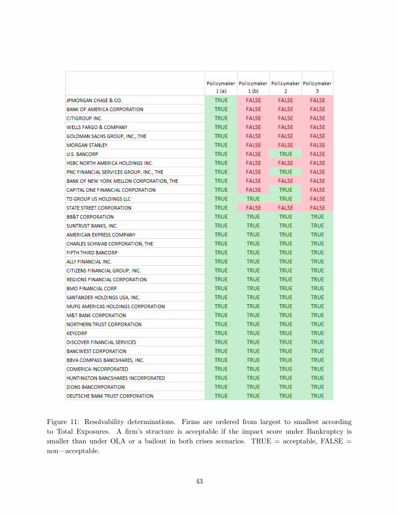
Figure 11: Resolvability determinations. Firms are ordered from largest to smallest according

to Total Exposures. A firm’s structure is acceptable if the impact score under Bankruptcy is

smaller than under OLA or a bailout in both crises scenarios. TRUE = acceptable, FALSE =

non–acceptable.

43

but it does carry a moral hazard impact as well. A simple way to rationalize this is to think of the

parameters of the linear function of size that is behind the score: the impact of size under OLA has

a lower slope, but a higher intercept, while the bailout score is independent of size. This implies

two thresholds in size that determine the firms that will be best resolved under bailout, OLA, and

bankruptcy.

It is interesting to compare our Policymaker 1(a) determination of adequate structure with the

determinations of the FDIC and the Board about the credibility of LWs. For the 2015 review

process, either the Board or the FDIC (or both) determined that the LWs of most of the firms

being reviewed that year had deficiencies important enough to fail the review process.39 Neither of

the two agencies found deficiencies in Citigroup’s LW. To square our results, which indicate that for

Policymaker 1(a) all firms have an acceptable structure, with the fact that these LW reviews found

deficiencies, it is necessary to recall that one important limitation of our exercise is that we lack

information on the “plan” in the LWs. As a result of this limitation, some deficiencies that are not

necessarily associated with characteristics cannot be captured in our impact score. For example,

one deficiency found in Bank of America’s LW was the failure to specify clear triggers under which

the parent company would provide liquidity to its subsidiaries, which is a plan item rather than a

firm characteristic that we can pick up in our financial—report—based score.40

As a final comment on our results, we want to emphasize again that our main contribution in

this paper is conceptual. The exercise presented in Figure 11 is just for illustration and our score

is far from being ready for policy use. More work is needed both to expand the list of scenarios

considered in it, to include any missing relevant characteristics of the firms, and to have the weights

be empirically based.

5.2 Comparison to the GSIB score

Another way of understanding what the new firm characteristics add to the determination of re-

solvability is to compare the ranking of firms according to the Basel GSIB score with our impact

score. We choose the comparison with the bankruptcy aggregate impact because that is likely to

be the assumption under which Basel understands the weights they use. Figure 12 presents the

results. The main differences in ranking are for smaller firms: while the GSIB score ranks them low,

the impact scores assign them more impact due to their relatively high numbers in the short-term

debt ratios and liquidity measures. This means that the smallest firm in the sample, Deutche Bank

Trust Corporation, is raked 13 out of 34 according to our impact score, while it was 34 under the

GSIB.

6 Extensions

In this section, we highlight a few other firm characteristics that would be relevant to calculate

the impact of a failure. These are characteristics that are difficult to measure and we leave their

39The list of firms whose LWs had deficiencies in 2015 is: Bank of America, Bank of New York Mellon, JP Morgan

Chase, State Street, Wells Fargo, Goldman Sachs, and Morgan Stanley.40Bank of America Living Will Feedback Letter (2016).

44

Figure 12: Comparison of the score and the ranking of firms according to the GSIB score and our

impact score, under two different policymaker’s weights.

45

inclusion in the impact score for future research: information on counterparties, data on network

structure, measures of impact outside of the financial system, legal complexity, core businesses and

services, and aspects of capital structure.

6.1 Information about counterparties

In the LWs, filers are asked to identify their “major counterparties . . . and describe the inter-

connections, interdependencies and relationships with such major counterparties.”41 Schedule B

(Interconnectedness Indicators) can be thought of as a “rough,” publicly available, measure of

these interconnections. Although privacy concerns must be taken into account, we think it would

be beneficial to construct, in the spirit of the LCR, a summary measure, based on average trades,

that captures the importance of the filing BHC to other financial institutions or to companies

outside of the financial system. For example, given that an individual firm knows to whom it is

lending and, and from these firms’ 10-Ks, the total amount of borrowing of each of its borrowers,

a firm could fairly easily estimate the percent of each of its major borrowers’ total funding that it

represents. Then, the firm could be required to report the total number of companies for which it

represents more than a threshold percent. Presumably, reporting of such a count would not reveal

private information.

6.2 Network structure

Even though there is information about the overall amount of interconnectedness in Schedule B, the

schedule ignores the network structure of counterparties, which is important for financial system

resilience in the event of failure (Allen and Gale, 2000). The recent literature on networks has

developed summary statistics that help characterize contagion propensity of different classes of

networks (see, for example, Gai and Kapadia, 2007). Including such statistics in the score, if

feasible, would be informative about contagion effects. Further work is necessary to establish the

optimal statistic and to deal with information revelation concerns.

6.3 Interconnectedness outside the financial system

We care greatly about contagion within the financial system because disturbances to the financial

system are thought to have a greater impact on economic output than disturbances in other sectors.

Accordingly, Schedule B is focused on capturing the direct impact of the failure of the reporting

firm for the financial system and holders of GSIB—issued securities. However, we think it would be

valuable to capture more generally the impact on the rest of the economy. At some level, the TE

measure can be thought of as a measure of potential contagion to all the economy, but nevertheless,

more specific information on the importance of a firm for the rest of the economy would be worth

collecting and including in the score. For example, we would estimate higher impact if the GSIB is

a major payments provider to a major nonfinancial firm or a major lender to the airline industry.

41“Federal Reserve System Reporting Requirements Associated with Regulation QQ (Resolution Plans Re-

quired), Model Template for §165(d) Tailored Resolution Plan.” January 31, 2016, p. 18. Available at:

https://www.federalreserve.gov/bankinforeg/resolution-plans/tailored-resolution-model-template.pdf.

46

6.4 Legal complexity, critical operations, and core businesses

We analyzed the feedback letters arising from the 2016 LW review process to look for firm char-

acteristics that were singled out as problematic for resolution (as opposed to shortcomings in the

plans for resolution). We found that regulators highlighted, in letters to several banks, an overly

complex legal entity structure (JP Morgan, State Street, and Wells Fargo). One concern, noted in

letters, is the location of entities in multiple jurisdictions. Another concern was the existence of

cross—guarantees, whereby a parent company bears unlimited liability for contracts created by its

subsidiaries. Such guarantees produce strong links between the solvency of different subsidiaries,

which may even be in different jurisdictions, and can create complications during resolution due

to the possibility of ring—fencing (whereby one jurisdiction prevents assets located within its bor-

der from being used to repay debt holders in a different jurisdiction). Given these examples, we

would expect a measure of this legal complexity to be included in the GSIB score; but no such

measure is incorporated, probably due to the difficulty constructing quantitative and informative

measures that can be comparable across firms and over time. This is an area of work that should

be prioritized when thinking about resolution.42

LWs also require firms to identify both the core businesses of the company and the critical oper-

ations that it performs for the financial system. While it appears that information regarding critical

operations is already captured in the GSIB score, we argue that information on core businesses is

not captured.

Critical operations are those, which, if shut down due to firm failure, would produce a strong

negative economic impact. To a large extent, the designation of critical operations is independent of

the firm’s structure and instead reflects the services provided to the economy. In our view, Schedule

C, Substitutability, which records the volume of payments, assets under custody, and underwriting

of securities, constitutes a reasonable measure of the importance of a firm’s critical operations.

Core businesses are defined as business lines and associated services that are important sources

of revenue for the firm. In the event of a wind down, knowing these sources could be helpful, so that

they can be protected as much as possible. As an example, IT for a whole BHC may be located in

one single subsidiary. In a scenario in which this particular subsidiary becomes insolvent, the most

orderly way of winding down the firm may involve using the parent company as a source of strength

for the troubled subsidiary, rather than enforcing firewalls (that are intended to prevent the spread

of the troubles of one subsidiary to others). It is clear that information about core businesses

should inform the “plan” included in LWs. In our example, a resolution plan that proposes to

sell a troubled subsidiary to minimize its impact on the remainder of the firm might not recognize

the importance of IT as a core business line or service. However, readiness for resolution as far as

core businesses protection is concerned could also be evaluated in the firm’s structure and hence

be captured in an impact score. In our example, if a BHC replicates IT services across subsidiaries

so that subsidiaries can be sold independently, in a resolution, this should translate into a lower

impact score. As with legal complexity, at this point, it is not clear in what way such information

could be incorporated into our quantitative impact score in an objective, general, and comparable

manner, but it may be an area for future attention.

42Schedule E provides minimal information on related ring-fencing concerns. See our discussion above.

47

6.5 Measuring the GSIB’s capability to recapitalize systemically important

subsidiaries

Another important aspect when evaluating the impact of a failure is the ability of the firm to

recapitalize systemically important subsidiaries using either an appropriate trigger for bankruptcy

(i.e., filing with enough capital buffer) or through the conversion of long—term debt into capital, as

mandated by TLAC. This ability to recapitalize depends both on whether maturity transformation

takes place at the parent company or at the subsidiaries (whether the BHC is “clean” or not,

according to TLAC requirements) and on the “plan” of resolution that the firms develop. A lack

of such ability to recapitalize has been pointed out as a source of deficiency in the evaluation of

LWs.43 The guidance for preparation of LWs issued by the Board and the FDIC in April of 2016

emphasized the need for both external and internal TLAC, as well as the need to pre—position

capital and liquidity in certain subsidiaries and to have governance arrangements in place such as

early bankruptcy triggers. These are all measures aimed at ensuring the ability of the failing firm

to recapitalize all subsidiaries that perform key services in the financial system.44

Current capital ratios may be informative about a firm’s ability to recapitalize subsidiaries that

provide critical services. However, for the purpose of our impact score, specific measures of capital

needs of each particular subsidiary may be desirable. As of now, using Y-15 data, we can only

construct a score at the BHC level. More work is needed to find publicly available data to construct

indicators of the structure of liquidity and capital across subsidiaries and parent companies.

7 Conclusion

Making the resolution of large, systemically important firms feasible without public support (i.e.,

making the firms “resolvable”) has been a priority in recent regulatory changes. One important

effort has centered on having firms describe in resolution plans (also known as living wills — LWs)

their structures and the means by which these structures, together with a wind—down strategy,

contribute to making unassisted bankruptcy the preferred method of resolution. The evaluation of

these LWs by regulators is complicated and has been deemed nontransparent to outsiders. In this

paper, we seek to develop tools, based on publicly available information, which can complement

the LW review process.

Our main contribution is to develop a conceptual framework to illustrate how to quantitatively

evaluate whether a firm is resolvable. We consider using a score that maps a firm’s financial data

into costs imposed on the economy – the impact – of resolving this failing firm via different

resolution methods and in different economic scenarios. For a given firm’s structure, bankruptcy

is preferable – from a certain policymaker’s point of view — to other resolution alternatives that

involve government support if the resulting impact calculated by the score is the lowest. Our

framework makes clear an important concept in the evaluation of LWs: though the failure of a

large firm is always going to be disruptive for the economy, the relevant question for resolvability

43See Board of Governors and FDIC (2016a).44See Board of Governors and FDIC (2016c).

48

is whether the extra losses stemming from unassisted resolution in bankruptcy are larger than the

moral hazard costs of providing support.

We discuss the data needs and difficulties of constructing such an impact score by proposing a

simplified two—scenario version of it. For this we use as a starting point the current Basel—developed

GSIB score. This score was created as a means of designating global banks as systemic and for

setting supplemental capital requirements. It measures how much economic damage a firm might

impose by its failure based on firm characteristics (financial data). We discuss each of the firm

characteristics included in the GSIB score and evaluate what failure costs each is meant to capture.

We supplement the original list of firm characteristics in the GSIB score with information on the

structure of debt of the firm, with emphasis on short—term debt and QFCs, as well as liquidity

measures. While our objective here is to measure resolvability, our modified score can also be

useful in thinking about refinements to this macro—prudential tool. Indeed, in what we think is

a step in the right direction, the revisions to the GSIB score for the U.S. implementation of the

capital surcharge that are being implemented in 2017 somewhat expand required disclosures on the

structure of short—term financing.

The moral hazard problem behind TBTF implies that, as long as firms put a positive probability

on assistance in some states of the world, they will have incentive to change their structure or

operations in ways that exploit the safety net. It follows from our analysis that the more realistic

and complete the set of scenarios the score considers, the more useful this instrument will be in

curbing the TBTF problem. In other words, expanding the set of scenarios may help policymakers

signal credibly that a firm will not be bailed out in a wide enough range of financial distress

scenarios so that creditors believe that the safety net will not protect them from losses under most

circumstances

To illustrate the concept of an impact score we compute the simplified two—scenario version of

our score with actual firm data and examples of how policymakers may evaluate impact. With

these examples, we seek to emphasize how the decisions to bail out a failing firm depend on

policymakers’ beliefs about how a given firm’s characteristics may translate into costs to society. In

practice, to make our score a positive tool (describing actual bailout decisions) or a normative tool

(evaluating the merits of different bailout policies) we would need empirical data from a number

of financial crises to determine the links between firm characteristics and impact from failure. Our

work highlights the need for future research along these lines.

References

[1] Allen, F., and D Gale (2000): “Financial Contagion,” Journal of Political Economy, 108(1),

1-33.

[2] Allen, F., and D Gale (1994): “Limited Market Participation and Volatility of Asset Prices,”

American Economic Review, 84(4), 933-955.

49

[3] Basel Committee on Banking Supervision, “Consultative Document. Global systemically im-

portant banks: Assessment methodology and the additional loss absorbency requirement”.

Available at https://www.bis.org/publ/bcbs201.pdf (2011)

[4] Board of Governors of the Federal Reserve System and Federal Deposit Insur-

ance Corporation. “Bank of America Living Will Feedback Letter for 2015.” (2016a)

Available at: https://www.federalreserve.gov/newsevents/pressreleases/files/bank-of-america-

letter-20160413.pdf

[5] Board of Governors of the Federal Reserve System and Federal Deposit Insurance Corporation.

“Resolution Plan Assessment Framework and Firm Determinations.” (2016b). Available at:

https://www.federalreserve.gov/newsevents/pressreleases/files/bcreg20160413a2.pdf

[6] Board of Governors of the Federal Reserve System and Federal Deposit Insurance Corpora-

tion. “Guidance for 2017 165(d) Annual Resolution Plan Submissions by Domestic Covered

Companies that Submitted Resolution Plans in July 2015.” (2016c)

[7] Board of Governors of the Federal Reserve System and Federal De-

posit Insurance Corporation. Joint Press Release. “Agencies announce

joint determinations for living wills.” December 19, 2017. Available at:

https://www.federalreserve.gov/newsevents/pressreleases/bcreg20171219a.htm

[8] Covitz, Daniel, Nellie Liang, and Gustavo A. Suarez (2013). “The Evolution of a Financial

Crisis: Collapse of the Asset-Backed Commercial Paper Market,” Journal of Finance, vol. 68,

no. 3, pp. 815-848.

[9] Diamond, D. and R. Rajan (2011): “Fear of Fire Sales, Illiquidity Seeking, and Credit Freezes,”

Quarterly Journal of Economics, 126(2) 557-591.

[10] Dodd—Frank Wall Street Reform and Consumer Protection Act; Regulatory Capital Rules:

Implementation of Risk—Based Capital Surcharges for Globally Systemically Important Bank

Holding Companies, 80 Fed. Reg. 49082 (August 14, 2015) (to be codified at 12 CFR pts. 208

& 217).

[11] Duffie, D. (2010) “How Big Banks Fail and What to Do about It”.

[12] Duffie, D. (2014) “Financial Market Infrastructure: Too Important to Fail” HOOVER INSTI-

TUTION, Economics Working Paper 14101

[13] Ennis and Price (2015), Discount Window Lending: Policy Trade-offs and the 1985 BoNY

Computer Failure, Economic Brief, Federal Reserve Bank of Richmond, May 2015, No. 15-05.

[14] Gai, P., and S. Kapadia: “Contagion in Financial Networks,” the Proceedings of the royal

Society of London, p.2401-2423 (2010).

[15] GAO. April 2016. “Resolution Plans”. http://www.gao.gov/assets/680/676497.pdf

50

[16] Hoenig, Thomas. March 2, 2015. “Remarks by Thomas M. Hoenig, Vice Chairman, Federal

Deposit Insurance Corporation: Financial Supervision: Basic Principles Presented to the In-

stitute of International Bankers Annual Washington Conference; Washington, DC”

[17] Jackson, Thomas H. July 9, 2014. “Building on Bankruptcy: A Revised Chapter 14 Proposal

for the Recapitalization, Reorganization, or Liquidation of Large Financial Institutions.” Man-

uscript, Stanford University.

[18] Jarque, Arantxa, and K. Athreya. “Understanding Living Wills”. Federal Reserve Bank of

Richmond Economic Quarterly, Third Quarter 2015.

[19] Kocherlakota, Narayana. “Taxing Risk and the Optimal Regulation of Financial Institu-

tions.” Economic Policy Papers. Federal Reserve Bank of Minneapolis. May 18, 2010. Avail-

able at: https://www.minneapolisfed.org/research/economic-policy-papers/taxing-risk-and-

the-optimal-regulation-of-financial-institutions.

[20] Krimminger, Michael H. “Does the Dodd-Frank Act End Too Big to Fail?” Statement be-

fore the Subcommittee on Financial Institutions and Consumer Credit; Financial Services

Committee; U.S. House of Representatives; Washington, D.C. June 14, 2011. Available at:

https://www.fdic.gov/news/news/speeches/archives/2011/spjun1411.html.

[21] Lacker, Jeffrey M., “Payment System Disruptions and the Federal Reserve Following Septem-

ber 11, 2001.” Journal of Monetary Economics 51, no. 5 (July 2004): 935-965.

[22] Lacker, Jeffrey M. “Economics After the Crisis: Models, Markets, and Impli-

cations for Policy.” Presentation before the Center for Advanced Study in Eco-

nomic Efficiency, Arizona State University. February 21, 2014. Available at:

https://www.richmondfed.org/press_room/speeches/jeffrey_m_lacker/2014/lacker_speech_20140221.

[23] Passmore, Wayne, and Alexander H. von Hafften (2017). “Are Basel’s Capital Surcharges

for Global Systemically Important Banks Too Small?,” Finance and Economics Discus-

sion Series 2017-021. Washington: Board of Governors of the Federal Reserve System,

https://doi.org/10.17016/FEDS.2017.021.

[24] Pellerin, Sabrina R. and John R. Walter. “Orderly Liquidation Authority as an Alternative to

Bankruptcy.” Federal Reserve Bank of Richmond, Economic Quarterly, First Quarter, 2012.

[25] Shleifer, Andrei, and Robert W Vishny. 2011. “Fire Sales in Finance and Macroeconomics.”

Journal of Economic Perspectives 25 (1): 29-48.

[26] Total Loss-Absorbing Capacity, Long-Term Debt, and Clean Holding Company Requirements

for Systemically Important U.S. Bank Holding Companies and Intermediate Holding Compa-

nies of Systemically Important Foreign Banking Organizations, 82 Fed. Reg. 8266 (January

24, 2017)

[27] Wells Fargo 2015 Living Will Feedback Letter. (2016)

51

[28] White, Phoebe and Tanju Yorulmazer, “Bank Resolution Concepts, Trade-offs, and Changes

in Practices”. Economic Policy Review, December 2014 Volume 20, Number 2

8 Appendix

8.1 Construction of short—term debt items in score

For the purpose of our examples of the impact score in the remainder of the paper, and because

data on Schedule G is not yet available, we construct our own measure of short—term borrowing

using Y-9C and Call Report data.45 In the following description of our calculations we provide the

item number for Y-9C figures in parenthesis.

• Short-term debt = commercial paper (bhck2309) + “Other borrowed money with a remainingmaturity of one year of less,” (bhck2332) + “fed funds and repo borrowings” (bhck3353, an

average over the last quarter) + uninsured deposits (collected from FDIC data for each

institution). Compared to the level of detail on short—term debt borrowing that the schedule

G gathers, our measure is fairly coarse. We are not able to break down short—term debt

by maturity or identify the portion of short—term debt emanating from within the financial

system. These are relevant details in the evaluation of the impact of failure. Once the revised

Y-15 form goes into effect, it may be feasible to refine our impact score using this detailed

information.

• QFCs = “fed funds and repo borrowings” (bhck3353, an average over the last quarter)

+ “derivatives purchased with negative fair value (“w.n.f.v.”)” (bhckc222) + derivatives

sold w.n.f.v. (bhckc220) + derivatives (interest rate swaps) w.n.f.v., traded (bhck8737)

and non—traded (bhck8745) + derivatives (foreign exchange) w.n.f.v., traded (bhck8738)

and non—traded (bhck8746) + derivatives (equity) w.n.f.v., traded (bhck8739) and non—

traded (bhck8747) + derivatives (commodities) w.n.f.v., traded (bhck8740) and nontraded

(bhck8748)

— Note that, ideally, we would want to leave out of the QFC measure the amount of fed

funds borrowings. However, measurements of only repo borrowings are only available

as an end-of-quarter measure, which is subject to window-dressing concerns (i.e., that

firms may substitute this form of borrowing only on the days in which their accounting

45The Y-9C, Consolidated Financial Statements for Holding Companies, is a regulatory report, collected by the

Federal Reserve gathers “basic financial data from a domestic bank holding company (BHC), a savings and loan

holding company (SLHC), a U.S intermediate holding company (IHC) and a securities holding company (SHC) on a

consolidated basis in the form of a balance sheet, an income statement, and detailed supporting schedules, including

a schedule of off balance-sheet items.” The Call Report, or more formally, Consolidated Reports of Condition and

Income, is completed by all U.S. banks and savings associations and is submitted to the Federal Financial Institutions

Examination Council, an interagency body representing the various U.S. banking supervisors. The Call Report gathers

detailed information on depository institution balance sheets, income statements, and off balance sheet items. The

Report includes a line item for “Estimated amount of uninsured deposits.”

52

information is used for regulatory filings, in order to get a more favorable capital re-

quirement). Hence, we use the entry for both fed funds borrowings and repos, which is

provided as an average over the quarter. Because in recent years fed funds borrowings

have been relatively low, we think this is a reasonable approximation.

• QFC/Assets: the above measure over “Total Assets” (bhck2170)

• Non—QFC—short—term debt = our above measure of short—term debt - “fed funds and repo

borrowings” (bhck3353, an average over the last quarter)

• Non—QFC—short—term debt ratio = our above measure of Non—QFC—short—term debt over

“Total Assets” (bhck2170)

• Inverse of Liquidity Coverage Ratio = our above measure of short—term debt over our measureof high-quality liquid assets (HQLA), following the classification used to compute the LCR,46

where

— HQLA = HQLA class 1 assets + 0.85 * HQLA class 2a assets, where, in turn,

— HQLA class 1 assets = hqla_1_1 (bhckd958) + hqla_1_2 (bhckd962) + hqla_1_3

(bhckd967) + hqla_1_4 (bhckd977),

— HQLA class 2a assets = hqla_2a_1 (bhck1295) + hqla_2a_2 (bhck1298) + hqla_2a_3

(bhckg305) + hqla_2a_4 (bhckg307) + hqla_2a_5 (bhckg379)

About the Repo measure: the list of QFCs includes repos, derivatives contracts such as swaps,

forwards, futures, and options. Because the Y-15 does not record separately the importance of

QFCs, we calculate our own measure using data from the Y-9C. Our calculation includes only

liability-related QFCs, because only GSIB liabilities can produce losses for creditors; so we include

repo borrowings and credit derivatives (sold or purchased) with a negative net value.

Although there are other types of derivatives that constitute a liability of the firm, beyond

those that we include in our calculation, only for these credit derivatives we can find their current

net value. Hence, we are underestimating the amount of liabilities in QFCs. Moreover, we have

no information about the maturity of the borrowing, or the liquidity of the collateral in these

contracts, which could be useful in considering their relative importance for contagion effects and

firesale concerns, as we argue below. This information will be collected by the revised Y-15, allowing

for future refinement of our impact score.

About the inverse LCR: while the mapping between liquidity classification (HQLA) from the

LCR regulation and firesale concerns is not unambiguous, it could act as a first approximation.

For Level 1 collateral (cash, central bank reserves, certain sovereign debt, and securities backed by

central banks) firesales are likely to be of little concern, because the total market volumes of Level

1 items are probably too large for a single institution to affect their price through a rushed sale. For

Level 2a assets (securities or debt issued by government agencies and riskier sovereign debt) and

46Data on the LCR for GSIBs and large foreign organizations are collected at high frequencies by regulators, but

they are not publicly available.

53

Level 2b assets (certain mortgage backed securities and corporate debt and equity), the concern

might be stronger, and probably, for our measure, we would be the most concerned with any debt

backed with assets with a rating below 2b. Because of this, we do not include them as HQLA.

The next tables present the scores we calculated for the 34 BHC in 2015, for each policymaker.

54

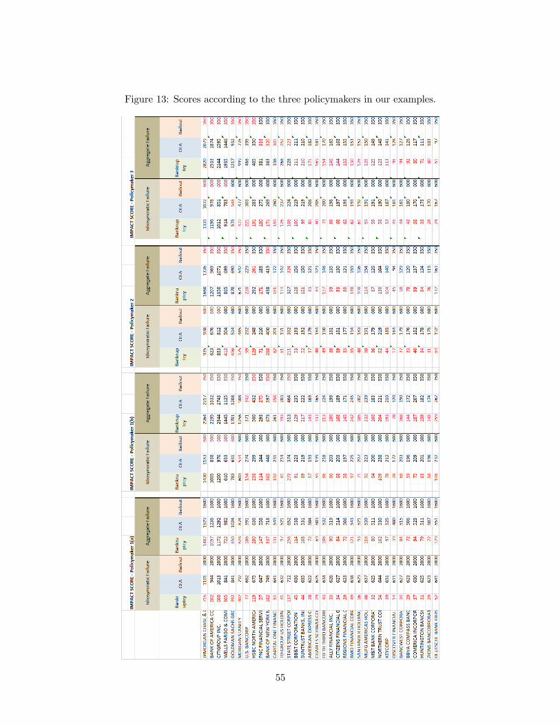
Figure 13: Scores according to the three policymakers in our examples.

55