Linear Programming in Linear Time When the Dimension Is Fixed

NIMROD MEGIDDO

Tel Aviv Universit~', Tel Aviv, Israel

Abstract. It is demonstrated that the linear programming problem in d variables and n constraints can be solved in O(n) time when d is fixed. This bound follows from a multidimensional search technique which is applicable for quadratic programming as well. There is also developed an algorithm that is polynomial in both n and d provided d is bounded by a certain slowly growing function of n.

Categories and Subject Descriptors: F.2.1 [Analysis of Algorithms and Problem Complexity]: Numerical Algorithms and Problems-computations on matrices; F.2.2 [Analysis of Algorithms and Problem Complexity]: Nonnumerical Algorithms and Problems-geometrical problems and computations; sort- ing and searching; G. 1.6 [Mathematics of Computing]: Optimization-linear programming

General Terms: Algorithms, Theory

Additional Key Words and Phrases: Genuinely polynomial time, multidimensional search, quadratic programming, smallest ball problem, linear time algorithms

1. Introduction

The computational complexity of linear programminghs one of the questions that has attracted many researchers since the invention of the simplex algorithm [3]. A major theoretical development in the field was Khachian's algorithm [7], which proved that the problem could be solved in time that is polynomial in the sum of logarithms of the (integral) coefficients. This notion of polynomiality is not alto- gether satisfactory (see [lo]), and, moreover, it is not expected that the algorithm will prove more practical than the simplex method. Khachian's result left an open question as to the existence of an algorithm that requires a number of arithmetic operations which is polynomial in terms of the size nd of the underlying matrix (where a' is the number of variables and n is the number of constraints). We call such an algorithm genuinely polynomial. This question is closely related to other interesting open questions in the theory of convex polytopes [6] concerning the diameter, height, etc., of polytopes. Obviously, Khachian's results has not advanced our knowledge about these problems.

With the central question still open, it is interesting to investigate special classes of linear programming problems. Systems of linear inequalities with no more than two variables per inequality have been shown by the author [13] to have a genuinely polynomial algorithm. When either n or d is fixed, then the simplex algorithm is

This work was supported in part by the National Science Foundation under Grants ECS-8 12 174 1 and ECS-8218181. Author's present address: Computer-Science Department, Stanford University, Stanford, CA 94305. Permission to copy without fee all or part of this material is granted provided that the copies are not made or distributed for direct commercial advantage, the ACM copyright notice and the title of the publication and its date appear, and notice is given that copying is by permission of the Association for Computing Machinery. To copy otherwise, or to republish, requires a fee and/or specific permission. @ 1984 ACM 0004-541 1/84/01 00-01 14 $00.75

Journal of the Association for Computing Machinery, Vol. 31, No. I, January 1984, pp. 114-127.

Linear Programming When Dimension Is Fixed 115

of course genuinely polynomial (while Khachian's algorithm is not). However, the crude bound of O(nd) (assuming d < n) means that no matter how slowly the dimension grows, we have a superpolynomial bound. Even the more refined bound of O(nC''') (see [8]) does not help in this respect. Here we develop an algorithm that is genuinely polynomial even if d grows slowly with n.

In this paper we study the complexity of linear programming in a fixed space. In other words, considering linear programming problems of n constraints in Rd, we study the asymptotic time complexity with respect to n for any fixed value of d. Surprisingly, this turns out to be linear in n, the coefficient of proportionality rapidly growing with d. We remark that in the worst case any version of the simplex algorithm requires O(n) time per pivot and hence is at least quadratic in terms of n even in the two-dimensional case. Our result implies a genuinely polynomial bound for classes of linear programs, where the dimension grows slowly with n, namely, d = log nlloglog n)'I2).

Our results rely on a novel multidimensional search technique developed in the present paper. One version of it may be described roughly as follows: to search relative to n objects in d space, we solve, recursively, two problems each with n/2 objects in (d - 1) space and then our problem is reduced to one with n/2 objects in d space. This should not be confused with Bentley's multidimensional divide- and-conquer [2], where an n x d problem is reduced to solving two (1112) x d-problems and then one n x (d - 1) problem.

We note that even though the results of this paper are interesting from the theoretical point of view in the general case, they are very practical for a small number of dimensions. In a previous paper [I21 the cases of d = 2 and 3 were described, and other classical problems were shown to suc,cumb to the same method of solution. Essentially, some of the common single-facility location problems relative to either the Euclidean or the rectilinear metric are solvable by this technique. Current computational experience with d = 3 looks very successful. Direct applications of linear programming in which the dimension is normally small are the following:

(1) Linear separability. Given n points in Rd, organized in two disjoint sets, find a hyperplane (if there is one) that separates the two sets. This problem is useful in statistics and in pattern recognition [4, 141.

(2) Chebyshev approximution [16]. Given n points a, = (a,l, . . . , u,d) E Rd (i = 1, . . . , n), we wish to find a linear function

so as to minimize max( 1 c$,' a,a,, + a d - u,d I : i = 1, . . . , n). For other related problems see [18]. We also note that the results can be extended to solve minimi- zation convex quadratic programming problems. For the details of the extension to quadratic programming, as well as other related problems solvable by similar techniques, the reader is referred to [ 121. Thus, the problem of finding the smallest ball enclosing n points in Rd can be solved in O(n) time for fixed d.

We start with an overview of the method, given in Section 2. In Section 3 we describe two closely related methods of multidimensional techniques, based on an oracle that can decide the "correct" side of any given hyperplane, relative to the point we are looking for. The applications of these abstract search techniques to linear programming are described in Section 4, where we discuss the linear programming oracle. The final estimations of time efforts are given in Section 5.

I 16 NIMROD MEGIDDO

2. An Overview We are interested in solving a d-dimensional linear programming problem of n constraints:

d

minimize C cJx, j= 1

d

so that 1 aijxj r b; (i = 1, . . . , a). j= 1

It is well known [3] that usually only relatively few constraints are tight at the optimal solution and hence, if we could identify those active constraints, we could solve our problem by solving a set of equations. The fundamental idea of our algorithm is to repeatedly reduce the set of constraints until the problem can be solved directly. For this idea to be successful, we need to drop relatively many constraints simultaneously. Fortunately, there is a way to drop a fixed fraction of the set of constraints regardless of the size of that set.

For the convenience of the presentation, let us transform the problem into the form

minimize xd

where ( II ( + ( I2 ( + ( I 3 ( = n. This transformation is always possible. (Set Z = C c,xj; eliminate xd; rename Z to be xd.) In other words, our problem is

minimize xd so that xd h maxi2 sox, + b,:i E I l l ,

xd 5 min(C ajjxj + bi:i E 12), max{C aijxj + bi:i E 13) 5 0.

It should be noted that the transformation is made only for the convenience of presentation. It merely reflects our consideration of the behavior of constraints in a subspace orthogonal to the gradient of the objective function. Repeated transfor- mations might cause difficulties from the point of view of numerical analysis. However, the algorithm can be programmed with no transformations.

Consider a pair of inequalities with indices i, k in the same set I, (1 I v I 3). For example, suppose ( 1, 2) C I I and consider the constraints xd r C$f a l j ~ j + b, and X(I r C$/ a ~ j x j + b2. The relationship between these two constraints can be summarized as follows:

(1) If (al I , . . . , = (a21, . . . , a2,d-I), then one of the constraints is redundant and can readily be dropped.

(2) If (a1 ,, . . . , a ~ , d - ~ ) # (a2 I , . . . , a2,+1), then the equation (I- I d- 1

C aljxj + b~ = 1 azjxj + b2 j= 1 j= 1

Linear Programming When Dimension Is Fixed 117

describes a hyperplane in R"-' which divides the space into two domains of domination; namely, on one side of this hyperplane C$,' al,x, + bl < C$! + bZ, whereas on the other side the reverse inequality prevails. Thus, if we could tell on what side of this hyperplane the optimal solution lies, then we could drop one of our constraints.

In general, the task of finding out on what side of a hyperplane the solution lies is not so easy, and we are certainly not going to test a hyperplane merely for dropping one constraint. We test relatively few hyperplanes, and our particular method of selecting those hyperplanes enables us to drop relatively many con- straints. This seems paradoxical; however, by carefully choosing the hyperplanes we can know the outcomes of tests relative to many other hyperplanes without actually performing those tests. We can summarize the characteristics of the method in general terms as follows. Given n inequalities in d variables, we test a constant number of hyperplanes (i.e., a number that is independent of n but does depend on the dimension) as to their position relative to the optimal solution. A single test amounts to solving up to three (d - 1)-dimensional linear programs of n constraints. Given the results of the tests for B-n pairs of inequalities (where 0 < B 5 4 is a constant independent of n but dependent on d), we can tell which member of the pair may be dropped without affecting the optimal solution. At this point the problem is reduced to a d-dimensional linear programming problem of (1 - B) . n constraints, and we proceed recursively.

For the complete description of the algorithm, we need to specify the following things. We need to explain what we mean by testing a hyperplane and we have to design an algorithm for a single test. Then we have to design the organization of the tests so as to establish a complete linear programming algorithm. These issues are discussed separately in the following sections. In Section 3 we discuss an abstract multidimensional search problem which we believe may also be applicable to problems other than linear programming. The implementation for linear pro- gramming is then discussed in Section 4.

3. A Multidimensional Search Problem

3.1 THE PROBLEM. Consider first a familiar one-dimensional search problem. Suppose there exists a real number x* which is not known to us; however, there exists an oracle that can tell us for any real number x whether x < x*, x = x*, or x > x*. Now, suppose we are given n numbers xi , . . . , x,, and we wish to know the position of each of them relative to x*. The question is how many queries we need to address the oracle (and also what is the other computational effort) in order to tell the position of each x, relative to x*. Obviously, we may sort the numbers in O(n1ogn) time and then perform a binary search for locating x* in the sorted set. This amounts to O(1ogn) queries. An asymptotically better performance is obtained if we employ a linear-time median-finding algorithm [ l , 171. We can first find the median of xi's, inquire about its position relative to x*, and then drop approximately one-half of the set of the xi's and proceed recursively. Thus, one query at the appropriate point suffices for telling the outcome with respect to half of the set. This yields a performance of O(n) time for median finding in sets of cardinalities n, n/2, 4 4 , . . . plus O(logn) queries. It is also important to note that a practical version of this idea is as follows. Pick a random xi and test it. Then drop all the elements on the wrong side and pick another element from a uniform distribution over the remaining set. This approach also leads to the expected

118 NIMROD MEGIDDO

number of O(1ogn) queries and O(n) comparisons. An analysis of essentially the same thing appears in [9j. An even more efficient idea is to select the median of a random sample of three or five.

We now generalize the one-dimensional problem to higher dimensions. Suppose that there exists a point x* E ~"h ich is not known to us, but that there is an oracle that can tell us for any a E Rd and a real number b whether aTx* < b, aTx* = b, or aTx* > b. In other words, the oracle can tell us the position of x* relative to any hyperplane in Rd.

Suppose we are given n hyperplanes and we wish to know the position of x* relative to each of them. The question, again, is how many queries will we need to address the oracle and what is the other computational effort involved in finding out the position of x* relative to all the n given hyperplanes? The general situation is of course extremely more complicated than the one-dimensional case. The major difference is that in higher dimensions we do not have the natural linear order that exists in the one-dimensional case. It is therefore quite surprising that the result from the one-dimensional case generalizes to higher dimensions in the following way. We show that for every dimension d there exists a constant C = C(d) (i.e., C is independent of n) such that only C-logn queries suffice for determining the position of x* relative to all the n given hyperplanes. There is naturally some additional computational effort involved, which turns out to be proportional to n (linear time), the coefficient of proportionality depending on d.

3.2. THE SOLUTION. The procedure that we develop here is described recur- sively. The underlying idea is as follows. We show that for any dimension d there exist constants A = A(d) (a positive integer) and B = ,B(d) (0 < B s i), which are independent of n, such that A queries suffice for determining the position of x*, relative to at least Bn hyperplanes out of n given ones in Rd. The additional computational effort is linear in terms of n. Given that this is possible, we can drop Bn hyperplanes and proceed recursively. Each round of A queries reduces the number of remaining hyperplanes by a factor of 1 - B. Thus, after approximately 10g,,,,_~,n rounds we will know the position of x* relative to all the hyperplanes. Thus the total number of queries is O(1ogn). The other computational effort amounts to cn + c(l - B)n + c(l - B)* + , which is no more than (c/B).n, and hence linear in terms of n.

The constants A and B are derived recursively with respect to the dimension. We already know that when d = 1, we can inquire once and drop half of the set of hyperplanes. We may therefore define A(l) = 1, B(l) = $. Henceforth, we assume d r 2.

Let H, = (x E R"aTx = b,) (i = 1, . . . , n) be n given hyperplanes (where a, = (a,,, . . . , a,d)T # 0 and bi is a real number, i = 1, . . . , n). We first note that it will be convenient (for the description of the procedure) to transform the coordinate system. Of course, we cannot transform the unknown point x*, but we can always transform a hyperplane back to the original system before asking the oracle about the position of the hyperplane. More precisely, if a vector x E Rd is represented as x = My, where M is a (d x d) nonsingular matrix, then a hyperplane aTx = b is represented by (aTM)y = b, and we may work with the vectors a ' = W a . If we need to inquire about a hyperplane afTy = b, then we look at aTx = b, where aT = a r T ~ - I

We would like to choose the coordinate system so that each hyperplane intersects the subspace of x, and x2 in a line (i.e., the intersection should be neither empty nor equal to the entire subspace). Since we have a finite number of hyperplanes, it

Linear Programming When Dimension Is Fi.xcd 119

is always possible to achieve this situation by applying a nonsingular transforma- tion. Specifically, we would like to have (a,, , a , ~ ) f (0, 0 ) for every 1 (i = 1, . . . , n). It is possible to find (in O(n) time) a basis for R5elative to which a,, # 0 for all i, j. This is based on the observation that v = v(c) = (1, t , c2 , . . . , c " ' ) ~ is orthogonal to some a, for at most n(d - 1 ) values of t . Using this observation, we can successively select our basic vectors so that none is orthogonal to any a,. Alternatively (just for arguing that the linear-time bound is correct), in order to avoid repeated transformation of this kind, we can say that we can simply ignore those hyperplanes with all = a12 = 0; if there are too many of them, then we can simply select variables other than x l and x2, and if the same trouble arises with every pair, then the entire situation is extremely simple (i.e., many constraints with only one positive cofficient a,,).

Now, each hyperplane H, intersects the ( x l , x2) subspace in a straight line a, ,xl + a,?x2 = b,. We define the slope of HI to be the slope of that straight line. More precisely, this slope equals +m if alz = 0 and -al l /aIz if a,2 # 0. We would like at least half of our hyperplanes to have a nonnegative slope and at least half of them to have a nonpositive slope. This can be achieved by a linear transformation of the ( x 1 , .r2) subspace. In particular, we may find the median of the set of slopes and apply a linear transformation that will take this median slope to zero. The transformation takes linear time and in fact is needed here only for simplicity of presentation. The algorithm can be programmed so that the same manipulations are applied to the original data. Thus, assume for simplicity of presentation that the original coefficients satisfy this requirement.

The first step in our procedure is to form disjoint pairs of hyperplanes where each pair has at least one member with a nonnegative slope and at least one member with a nonpositive slope. We now consider the relationship between two members of a typical pair. Suppose, for example, that H, has a nonnegative slope, while Hh has a nonpositive slope, and that we have matched H, with Hk. Assume, first, that the defining equations of H, and HA are linearly independent. Let Hji' denote the hyperplane defined by the equation

d

C (ah~a , - a , ~ a ~ , ) x , = a ~ l b , - a , ~ h ~ .

This equation is obtained by subtracting all times the equation of Hk from akl times the equation of H,. Thus, the intersection of H,, Hk and Hjj' is ( d - 2) dimensional. Moreover, the coefficient of x l in Hj;' is zero. This property is essential for our recursive handling of hyperplanes of the form of HI;), which takes place in a lower dimensional setting. Analogously, let Hj;' denote the hyperplane defined by

d

1 (akza,, - a,2ak,)x, = a k h - a,2bk. j= I

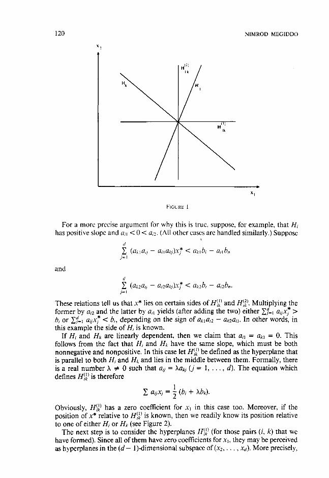
The hyperplane Hj:' has characteristics similar to those of Hjl'. To understand the significance of HI:' and HI:', note that if we know the position of x* relative to both of these hyperplanes, then we can readily tell the position of x* relative to one of either HI or HL. This is illustrated in Figure I . Note that the intersection of the four hyperplanes is still (d - 2) dimensional, and their relative positions are fully characterized by their intersection with the ( x l , x z ) subspace. The fact that H, and Hk have slopes of opposite signs is essential for our conclusion. If, for example, x* is known to lie to the "left" of HI:' and "above" Hj:', then we definitely know that it lies "northwest" of H,.

NIMROD MEGIDDO

For a more precise argument for why this is true, suppose, for example, that HI has positive slope and all < 0 < a12. (All other cases are handled similarly.) Suppose

d

1 ( a ~ ~ a , , - a , ~ a ~ ~ ) x , * < aklbl - allb,, J= I

and

These relations tell us that x* lies on certain sides of H$) and H$). Multiplying the * former by ail and the latter by ail yields (after adding the two) either Cgl a,,x, > b; or zf=l ajjx; < bi, depending on the sign of akla;;! - ak2ail. In other words, in this example the side of Hi is known.

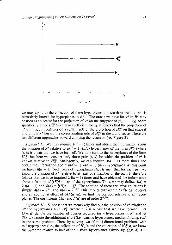
If Hi and Hk are linearly dependent, then we claim that ail = akl = 0. This follows from the fact that Hi and Hk have the same slope, which must be both nonnegative and nonpositive. In this case let HI;' be defined as the hyperplane that is parallel to both Hi and Hk and lies in the middle between them. Formally, there is a real number X # 0 such that aij = Xakj ( j = 1 , . . . , d). The equation which defines HI:) is therefore

Obviously, HI;) has a zero coefficient for x l in this case too. Moreover, if the position of x* relative to H$) is known, then we readily know its position relative to one of either H, or Hk (see Figure 2).

The next step is to consider the hyperplanes HI:' (for those pairs (i, k) that we have formed). Since all of them have zero coefficients for X I , they may be perceived as hyperplanes in the (d - 1)-dimensional subspace of ( ~ 2 , . . . , xd). More precisely,

Linear Programming When Dimension Is Fixed

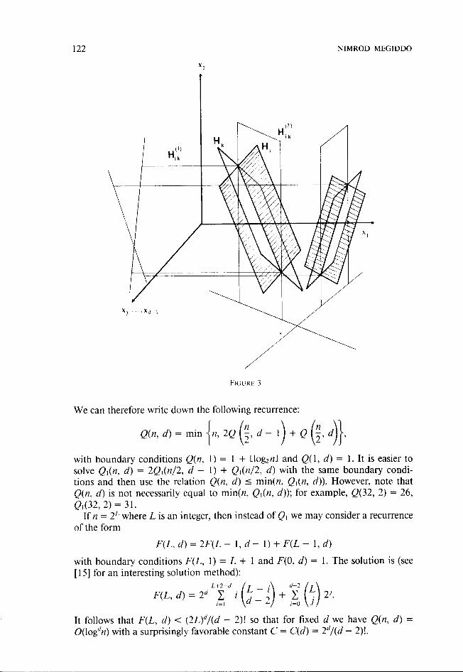
we may apply to the collection of these hyperplanes the search procedure that is recursively known for hyperplanes in Rd-I. The oracle we have for x* in Rd may be used as an oracle for the projection of x* on the sutppace of ( ~ 2 , . . . , xd). More specifically, since HI:' has a zero coefficient for XI , it follows that the projection of x* on ((xZ, . . . , xd)) lies on a certain side of the projection of HI:) on that space if and only if x* lies on the corresponding side of HI:' in the grand space. There are two different approaches toward applying the recursion (see Figure 3):

Approach I. We may inquire A(d - 1) times and obtain the information about the position of x* relative to B(d - l).(n/2) hyperplanes of the form H'.:.' (where (i, k) is a pair that we have formed). We now turn to the hyperplanes of the form H!:), but here we consider only those pairs (i, k) for which the position of x* is known relative to HI;). Analogously, we can inquire A(d - 1) more times and obtain the information about B(d l).B(d - l).(n/2) hyperplanes. At this point we have (B(d - 1))2(n/2) pairs of hyperplanes Hi, Hk such that for each pair we know the position of x* relative to at least one member of the pair. It therefore follows that we have inquired 2A(d - 1) times and have obtained the information about a fraction of i(B(d - of the hyperplanes. Thus, we may define A(d) = 2A(d - 1) and B(d) = i(B(d - The solution of these recursive equations is simple: A(d) = 2"' and B(d) = 21-2d. This implies that within C(d).logn queries and an additional effort of O(F(d)-n), we find the position relative to all hyper- planes. The coefficients C(d) and F(d) are of order 2•‹(2d).

Approach II. Suppose that we recursively find out the position of x* relative to all the hyperplanes HI;), HI:) (where i, k is a pair that we have formed). Let Q(n, d) denote the number of queries required for n hyperplanes in R h n d let T(n, d) denote the additional effort (i.e., pairing hyperplanes, median finding, etc.) in the same problem. Then, by solving two (d - 1)-dimensional problems with n/2 hyperplanes (i.e., the collection of H$:)'s and the collection of H$:)'s), we know the outcome relative to half of the n given hyperplanes. Obviously, Q(n, d) I n.

NIMROD MEGIDDO

We can therefore write down the following recurrence:

with boundary conditions Q(n, 1) = 1 + LlogznJ and Q(1, d ) = 1. It is easier to solve Ql(n, d) = 2Ql(n/2, d - 1) + Ql(n/2, d ) with the same boundary condi- tions and then use the relation Q(n, d ) 5 min(n, Ql(n, d)). However, note that Q(n, d ) is not necessarily equal to min(n, Ql(n, d)); for example, Q(32, 2) = 26, Ql(32, 2) = 3 1.

If n = 2L where L is an integer, then instead of Q, we may consider a recurrence of the form

with boundary conditions F(L, 1 ) = L + 1 and F(0, d) = 1. The solution is (see [15] for an interesting solution method):

It follows that F(L, d) < ( 2 ~ ) ~ / ( d - 2)! so that for fixed d we have Q(n, d ) = O(logdn) with a surprisingly favorable constant C = C(d) = 2d/(d - 2)!.

Linmr Programming When Dimension Is Fixed

The other effort involved in preparations for queries satisfies

T(n, d ) 5 2 T -, d - 1 + T -, d + fl(nd).

Consider the recurrence

(I' ) I ' ) F(L, d ) = 2 F ( L - 1, d - 1 ) + F(L- 1 , d ) + 2 L d

with boundary conditions F(0, d) = 1 and F(L, 1) = 2L. Surprisingly, this turns out to be linear in 2L for every fixed d, with constants C(d) that satisfy C(d) r 2(C(d - 1) + d). Thus T(n, d ) < d2d-n.

It thus appears that the second approach may be more practical than the first, provided n is not extremely large relative to d. These two different approaches to multidimensional search give rise to two different algorithms for the linear pro- gramming problem. These algorithms are discussed after we provide the details of the oracle for linear programming.

4. The Oraclejbr Linear Programming

In this section we specify what we mean by testing a hyperplane in R ~ . We first define what we require from a procedure for linear programming.

Given a d-variable linear programming problem d

minimize 1 cjxj ] = I

d

so that 2 a,,xj 2 bi (i = 1, . . . , n), J= I

we require that the procedure either provide an optimal solution, report that the problem is unbounded, or (in case the problem is infeasible) provide a vector x' =

d (xl, . . . , x j ) which minimizes the function Axl, . . . , xd) = max(bi - alixj:i = 1, . . . , n). Note that the requirement in case the problem is infeasible is rather unusual; it is needed here for recursive purposes.

The procedure we have developed so far solves this extended notion of a linear programming problem, provided we have a suitable oracle. Specifically, when given a hyperplane xj'=l ajx, = h, we need to know one of the following:

( 1 ) The hyperplane contains the final outcome; that is, either there is an optimal solution on the hyperplane, the problem is unbounded even on the hyperplane, or the hyperplane contains a minimizer of the function f:

(2) The final outcome is on a certain side of the hyperplane. However, in this case we do not expect to know the nature of the final outcome, that is, whether the problem is feasible and bounded.

We have to clarify that such an approach is valid even if the linear programming problem has multiple optima. This follows from convexity of the set of optimal solutions. If the hyperplane does not contain an optimal point (i.e., a point that may be interpreted as x*), then all optimal points lie on one side of the hyperplane (i.e., the oracle will respond in the same way for all possible choices of x* in the optimal set).

We now show that the oracle is no more than a recursive application of the master problem (i.e., the extended linear programming problem discussed earlier in this section) in a lower dimensional space.

124 NIMROD MEGIDDO

Given the linear programming problem and the hyperplane, we first consider the same problem with the equalion of the hyperplane as an additional constraint. This is a d-variable problem of n + 1 constraints, but we can eliminate one variable and thus have an equivalent (d - 1)-variable problem of n constraints. Moreover, for simplicity of presentation we may assume that the given hyperplane is simply ],u,/ = 0). (Otherwise, apply an affine transformation that takes the given hyperplane to the latter.) Thus the (d - 1)-dimensional problem is obtained by dropping the variable ,Q. We assume of course that d r 2; the case d = 1 is easy since then the "hyperplane" is a single point. If the problem is feasible and unbounded even when confined to (xd = 0), we are done. Otherwise, we obtain (recursively) either an optimal solution x* = (xT, . . . , x$-], 0) (optimality is relative to (xd = 0)) or a vector x' = (XI, . . . , xLl , 0) which minimizes the function f on (xd = 0). We now need to determine whether we already have the final outcome or, alternatively, which side of (xd = 01 should be searched. Distinguish two cases:

Case I. First consider the case in which we obtain an optimal solution x*. We would like to know whether there exists a vector y = ( y l , . . . , y d ) such that yd > 0, C cJ y, < C cJx; and C a,,yJ r b, (i = I, . . . , n). Convexity of the feasible domain and linearity of the objective function imply that if a vector y satisfies these requirements, then so does the vector ( 1 - t)x* + ty for any t (0 < t 5 1). It is therefore sufficient to look only in the neighborhood of x*. Specifically, consider the following (d - I)-dimensional problem:

d- I

minimize 1 cJxJ /= 1 * d- l

so that 1 a,,xJ + a , d 2 0 (i E I), j=1

where I = (i:C ~ , ~ x J k = b,). Here we impose only those constraints that are tight at x* and we set xd = 1. This is because we are interested only in the local behavior in the neighborhood of x* and we wish to determine the existence of a direction of improvement. It is easy to see that this (d - 1)-dimensional problem has a solution with a negative objective-function value if and only if there is a direction with the following property: Moving from x* in that direction into the half-space (xd > 01, we remain in the feasible domain if the move is sufficiently small (yet positive) while the objective function decreases. Thus, if the problem is infeasible or if, in turn, its optimal value is nonnegative, then there is nothing to look for in that half- space. In the latter case we then consider the other half-space by solving the following problem:

d- l

minimize 1 cJxJ ,I= I

d- l

so that C a,x, - u , ~ 2 0 (i E I). j= I

Analogously, the half-space (xd < 0) contains solutions that are better than x* if and only if this problem has a solution with a negative objective-function value. We note that since x* is a relative optimum, it follows that at most one of these auxiliary problems can have a solution with a negative objective-function value. If neither has solutions with negative values, then x* is a global optimum and we are done with the original problem.

Linear Programming When Dimension Is Fixed 125

Case II. The second case is that in which the problem is infeasible on the hyperplane (xd = 0). Here we obtain a vector x ' = (x', . . . , x k l , 0) that mini- mizes the function f(xl, . . . , xd) (defined above) on {xd = 0). Note that this function is convex so that it is sufficient to look at the neighborhood of x ' in order to know which half-space may contain a feasible point. Formally, let I' = (i:f(x;, . . . , x k l , 0) = b, - C?:: ajjxj ). We are now interested in the following questions:

QI. Is thereavectory=(yl , . . . , y d ) suchthatyd>Oand d

X auyj > 0 for i E I f ? j= 1

Q2. Is there a vector z = (zl, . . . , zd) such that zd < 0 and d

ajjzj > 0 for i € I '? j- 1

Note that if the answer to Ql is in the affirmative, then we proceed into the half- space (xd > 0); if the answer to 4 2 is in the affirmative, then we proceed into {xd < 0); if both answers are in the negative, then we conclude that the original problem is infeasible and that x' is a global minimum of the function f:

We answer the above questions in a somewhat tricky way. Consider the following (d - 1)-dimensional problem:

minimize 0 d- I

so that 1 auyj r -aid (i € 1'). j= 1

If this problem is feasible, then there is a vector y such that yd > 0 and Cgl aij yj r 0 (i E 1'). We claim that in this case the answer to Q2 is in the negative. This follows from the fact that if there is also a vector z such that zd < 0 and Cj'=l a,,zj > 0 (i E 1'), then there is a vector x such that xd = 0 and for i E 1', C,d,l auxj > 0 (x is a suitable convex combination of y and z); and this contradicts the assumption that x' minimizes the function f: Similarly, if there is a vector z such that Cj'zf aijzj r aid (i E 1'), then the answer to Q1 is in the negative. Thus, the procedure in the present case can be summarized as follows. We consider two sets of inequalities in d - 1 variables:

If both (1) and (2) are feasible or infeasible, then we conclude that x' is a global minimum of the function f and the original problem is infeasible. If precisely one is feasible, then we proceed into the half-space corresponding to the other one; that is, if (1) is the feasible one, we proceed into (xd < 0), whereas if (2) is the feasible one, we proceed into (xd > 0).

This completes the description of what the oracle does. We note that the oracle may need to solve three (d - 1)-dimensional problems

of (possibly) n constraints each. However, the number of constraints is usually

126 NIMROD MEGIDDO

much smaller in two of the problems. More precisely, the cardinality of the sets I and I' is not greater than d if we assume nondegeneracy [3]. So, two of the three problems the oracle needs to solve are rather easy.

5. Conclusion

If Approach I is used for the multidimensional search, then by solving not more than 3.2"' problems of order n x (d - I), we reduce a problem of order n x d to a problem of order n(1 - 2'-Id) x d. Hence the total effort LP,(n, d) using this approach satisfies

LPl(n, d) s. 3 . 2d- '~P l (n , d - 1) + LPl(n(l - 2'-Id), d) + B(nd).

It can be proved by induction on d that for every d there exists a constant C(d) such that LP,(n, d) < C(d). n. It can further be seen that C(d) 5 3. 22d+d-2 l), which implies C(d) < 21d+'; that is, C(d) < 20'Iq'. It is interesting to compare this result with the epilogue in [a], where questions are raised with regard to the average complexity of the simplex algorithm as the number of variables tends to infinity while the number of constraints is fixed. The answer is highly sensitive to a probabilistic model to be adopted. Smale [19] has shown that, under a certain model, the average number of pivot steps is o(nf) for every t > 0 whenever the number of constraints is fixed.

Using Approach 11, we reduce a problem of order n x d to one of order (n/2) x d by solving O((2 10g(n/2))~/(d - 2)!) problems of order n x (d - I), incurring an additional effort of 0(d2~n). The resulting total effort satisfies

LP2(n, d) 5 c (210g(n'2))' ~ ~ 2 ( n , d - 1) ; L P ~ (:, d) + o(~z*). (d - 2)!

It can be proved that for fixed d, LP2(n, d) = O(n(logn)"*), with a rather unusual constant C(d) < 2dz/n&: k!

The argument that the worst case complexity is linear relies heavily on the fact that we can find the median in linear time. However the linear-time, median- finding algorithms [ 1, 171 are not altogether practical. In practice we would simply select a random element from the set of critical values rather than the median. It appears that the best practical selection is of the median of a random 3-sample or 5-sample. Since this is repeated independently many times, we do achieve expected linear-time performance (where the expectation is relative to our random choices). The analysis is close to that of algorithm FIND (see [9]). Another approach is to employ a probabilistic selection algorithm like that in [5], but, again, it is not required that the exact median be found.

Finally, we remark that a hybrid multidimensional search (i.e., picking, recur- sively, the better between the two approaches whenever a search is called for) may improve the bounds presented here.

ACKNOWLEDGMENTS. Fruitful discussions with Zvi Galil are gratefully acknowl- edged. The author also thanks the referees for their constructive comments.

REFERENCES

(Note. Reference [I I] is not cited in the text.) 1 . AHO, A.V., HOPCROFT, J.E., AND ULLMAN, J.D. The Design andAnalysis of Computer Algorithms.

Addison-Wesley, Reading, Mass., 1974. 2. BENTLEY, J.L. Multidimensional divide-and-conquer. Commun. ACM 23, 4 (Apr. 1980),

2 14-229.

Linear Programming When Dimension Is Fixed

3. DANTLIG, G.B. Linear Programming and Extensions. Princeton University Press, Princeton, N.J., 1963.

4. DUDA, R.O., AND HART, P.E. Pattern Classification and Scene Analysis. Wiley-Interscience, New York, 1973.

5. FLOYD, R.W., AND RIVEST, R.L. Expected time bounds for selection. Commun. ACM 18,3 (Mar. 1975), 165-172.

6. GRUNBAUM, B. Convex Polytopes. Wiley, New York, 1967. 7. KHACHIAN, L.G. A polynomial algorithm in linear programming. Soviet Math. Dokl. 20 (1979),

191-194. 8. KLEE, V., AND MINTY, G.J. How good is the simplex algorithm? In Inequalities, vol. 3. Academic

Press, New York, 1972, pp. 159-175. 9. KNUTH, D.E. Mathematical analysis of algorithms. In Information Processing 71. Elsevier North-

Holland, New York, 1972, pp. 19-27. 10. MEGIDW, N. IS binary encoding appropriate for the problem-language relationship? Theor.

Comput. Sci. 19 (1982), 337-341. I I. MEGIDW, N. Solving linear programming when the dimension is fixed. Dept. of Statistics, Tel

Aviv University, April 1982. 12. MEGIDDO, N. Linear-time algorithms for linear programming in R h n d related problems. SIAM

J. Comput. I2 ,4 (Nov. 1983). 13. MEGIDDO, N. Towards a genuinely polynomial algorithm for linear programming. SIAM J.

Comput. 12, 2 (May 1983), 347-353. 14. MEISEL, W.S. Computer-OrientedApproaches to Pattern Recognition. Academic Press, New York,

1972. 15. MONIER, L. Combinatonal solutions of multidimensional divide-and-conquer recurrences. J.

Algorithms I (1980), 60-74. 16. RICE, J. The Approximation of Functions. Vol. I; The Linear Theory. Addison-Wesley, Reading,

Mass., 1964. 17. SCHONHAGE, A., PATERSON, M., AND PIPPENGER, N. Finding the median. J. Comput. Syst. Sci.

13 (1976), 184-199. + 18. SHAMOS, M.I. Computational geometry. Ph.D. dissertation, Dept. of Computer Science, Yale

Univ., New Haven, Conn., 1978. 19. SMALE, S. On the average speed of the simplex method of linear programming. To appear in

Math. Program.

Journal of the Association for Computing Machinery, Vol. 31. No. I. January 1984.