Linear Programming, Lagrange Multipliers, and Duality

Geoff Gordon

lp.nb 1

Overview

This is a tutorial about some interesting math and geometry connected with constrained optimization. It is not primarily about algorithms—while it mentions one algorithm for linear programming, that algorithm is not new, and the math and geometry apply to other constrained optimization algorithms as well.

The talk is organized around three increasingly sophisticated versions of the Lagrange multiplier theorem:

• the usual version, for optimizing smooth functions within smooth boundaries,

• an equivalent version based on saddle points, which we will generalize to

• the final version, for optimizing continuous functions over convex regions.

Between the second and third versions, we will detour through the geometry of convex cones.

Finally, we will conclude with a practical example: a high-level description of the log-barrier method for solving linear programs.

lp.nb 2

Lagrange Multipliers

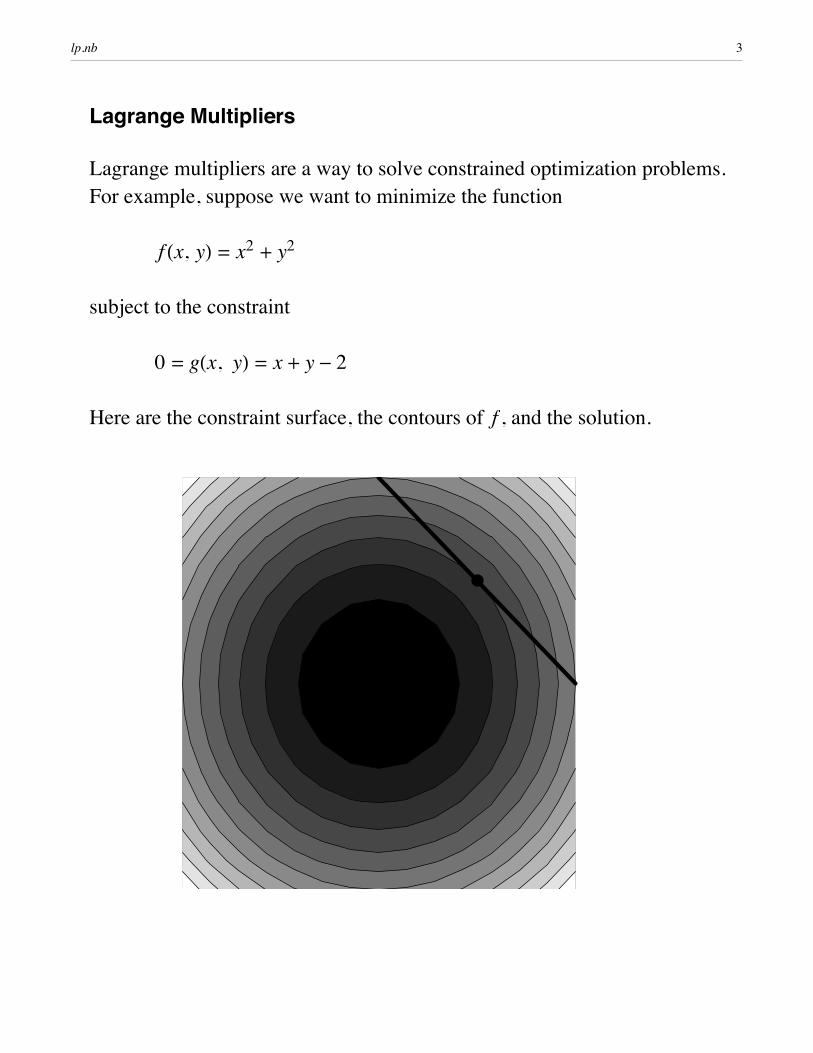
Lagrange multipliers are a way to solve constrained optimization problems. For example, suppose we want to minimize the function

f Hx, yL = x2 + y2

subject to the constraint

0 = gHx, yL = x + y- 2

Here are the constraint surface, the contours of f , and the solution.

lp.nb 3

More Lagrange Multipliers

Notice that, at the solution, the contours of f are tangent to the constraint surface. The simplest version of the Lagrange Multiplier theorem says that this will always be the case for equality constraints: at the constrained optimum, if it exists, “ f will be a multiple of “g.

The Lagrange Multiplier theorem lets us translate the original constrained optimization problem into an ordinary system of simultaneous equations at the cost of introducing an extra variable:

gHx, yL = 0“ f Hx, yL = p “gHx, yL

The first equation states that x and y must satisfy the original constraint; the second equation adds the qualification that “ f and “g must be parallel. The new variable p is called a Lagrange multiplier.

lp.nb 4

The Lagrangian

We can write this system of equations more compactly by defining the Lagrangian L:

LHx, y, pL = f Hx, yL + p gHx, yL = x2 + y2 + pHx + y- 2L

The equations are then just “L = 0, or in this case

x + y = 22 x = -p2 y = -p

The unique solution for our example is x = 1, y = 1, p = -2.

lp.nb 5

Multiple Constraints

The same technique allows us to solve problems with more than one constraint by introducing more than one Lagrange multiplier. For example, if we want to minimize

x2 + y2 + z2

subject to

x + y- 2 = 0x + z - 2 = 0

we can write the Lagrangian

LHx, y, z, p, qL = x2 + y2 + z2 + pHx + y- 2L + qHx+ z- 2L

and the corresponding equations

0 = “x L = 2 x + p + q0 = “y L = 2 y+ p0 = “z L = 2 z+ q0 = “p L = x + y- 20 = “q L = x + z - 2

lp.nb 6

Multiple Constraints: the Picture

The solution to the above equations is

9p Ø - 4ÅÅÅÅÅ3

, q Ø - 4ÅÅÅÅÅ3

, x Ø 4ÅÅÅÅÅ3

, y Ø 2ÅÅÅÅÅ3

, z Ø 2ÅÅÅÅÅ3=

Here are the two constraints, together with a level surface of the objective function. Neither constraint is tangent to the level surface; instead, the normal to the level surface is a linear combination of the normals to the two constraint surfaces (with coefficients p and q).

lp.nb 7

Saddle Points

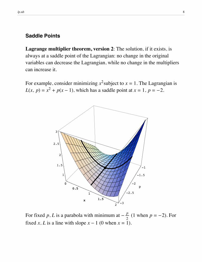
Lagrange multiplier theorem, version 2: The solution, if it exists, is always at a saddle point of the Lagrangian: no change in the original variables can decrease the Lagrangian, while no change in the multipliers can increase it.

For example, consider minimizing x2subject to x = 1. The Lagrangian is LHx, pL = x2 + pHx - 1L, which has a saddle point at x = 1, p = -2.

0

0.5

1

1.5

2x

-3

-2.5

-2

-1.5

-1

p

1

1.5

2

2.5

3

0

0.5

1

1.5x

For fixed p, L is a parabola with minimum at - pÅÅÅÅÅ2

(1 when p = -2). For fixed x, L is a line with slope x - 1 (0 when x = 1).

lp.nb 8

Lagrangians as Games

Because the constrained optimum always occurs at a saddle point of the Lagrangian, we can view a constrained optimization problem as a game between two players: one player controls the original variables and tries to minimize the Lagrangian, while the other controls the multipliers and tries to maximize the Lagrangian.

If the constrained optimization problem is well-posed (that is, has a finite and achievable minimum), the resulting game has a finite value (which is equal to the value of the Lagrangian at its saddle point).

On the other hand, if the constraints are unsatisfiable, the player who controls the Lagrange multipliers can win (i.e., force the value to +!), while if the objective function has no finite lower bound within the constraint region, the player who controls the original variables can win (i.e., force the value to -!).

We will not consider the case where the problem has a finite but unachievable infimum (e.g., minimize expHxL over the real line).

lp.nb 9

Inequality Constraints

What if we want to minimize x2 + y2subject to x + y- 2 ¥ 0?

We can use the same Lagrangian as before:

LHx, y, pL = x2 + y2 + pHx+ y- 2L

but with the additional restriction that p § 0.

Now, as long as x+ y- 2 ¥ 0, the player who controls p can't do anything: making p more negative is disadvantageous, since it decreases the Lagrangian, while making p more positive is not allowed.

Unfortunately, when we add inequality constraints, the simple condition “L = 0 is neither necessary nor sufficient to guarantee a solution to a constrained optimization problem. (The optimum might occur at a boundary.)

This is why we introduced the saddle-point version of the LM theorem. We can generalize the Lagrange multiplier theorem for inequality constraints, but we must use saddle points to do so.

First, though, we need to look at the geometry of convex cones.

lp.nb 10

Cones

If g1, g2, ... are vectors, the set 8ai gi » ai ¥ 0< of all their nonnegative linear combinations is a cone. The gi are the generators of the cone. The following picture shows two 2-dimensional cones which meet at the origin. The dark lines bordering each cone form a minimal set of generators for it; adding additional generating vectors from inside the cone wouldn't change the result.

These particular two cones are duals of each other. The dual of a set C, written C¶, is the set of all vectors which have a nonpositive dot product with every vector in C. If C is a cone, then HC¶L¶ = C.

lp.nb 11

Special Cones

Any set of vectors can generate a cone. The null set generates a cone which contains only the origin; the dual of this cone is all of —n. Fewer than n vectors generate a cone which is contained in a subspace of —n.

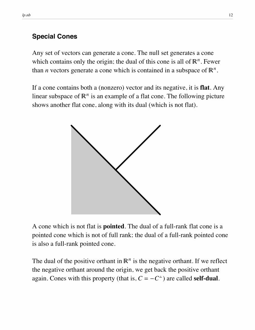
If a cone contains both a (nonzero) vector and its negative, it is flat. Any linear subspace of —n is an example of a flat cone. The following picture shows another flat cone, along with its dual (which is not flat).

A cone which is not flat is pointed. The dual of a full-rank flat cone is a pointed cone which is not of full rank; the dual of a full-rank pointed cone is also a full-rank pointed cone.

The dual of the positive orthant in —n is the negative orthant. If we reflect the negative orthant around the origin, we get back the positive orthant again. Cones with this property (that is, C = -C¶) are called self-dual.

lp.nb 12

Faces and Such

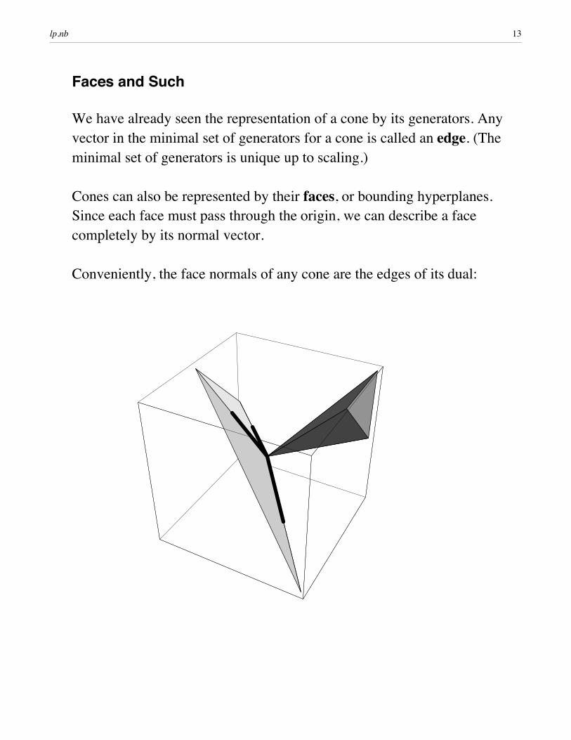
We have already seen the representation of a cone by its generators. Any vector in the minimal set of generators for a cone is called an edge. (The minimal set of generators is unique up to scaling.)

Cones can also be represented by their faces, or bounding hyperplanes. Since each face must pass through the origin, we can describe a face completely by its normal vector.

Conveniently, the face normals of any cone are the edges of its dual:

lp.nb 13

Representations of Cones

Any linear transform of a cone is another cone. If we apply the matrix A (not necessarily square) to the cone generated by 8gi » i = 1. .m<, the result is the cone generated by 8A gi » i = 1. .m<.

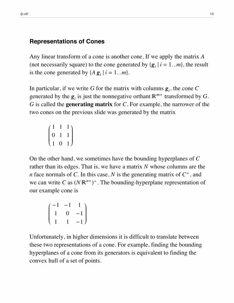
In particular, if we write G for the matrix with columns gi, the cone C generated by the gi is just the nonnegative orthant —m+ transformed by G. G is called the generating matrix for C. For example, the narrower of the two cones on the previous slide was generated by the matrix

i

k

jjjjjjj

1 1 10 1 11 0 1

y

{

zzzzzzz

On the other hand, we sometimes have the bounding hyperplanes of C rather than its edges. That is, we have a matrix N whose columns are the n face normals of C. In this case, N is the generating matrix of C¶, and we can write C as HN —n+L¶. The bounding-hyperplane representation of our example cone is

i

k

jjjjjjj

-1 -1 11 0 -11 1 -1

y

{

zzzzzzz

Unfortunately, in higher dimensions it is difficult to translate between these two representations of a cone. For example, finding the bounding hyperplanes of a cone from its generators is equivalent to finding the convex hull of a set of points.

lp.nb 14

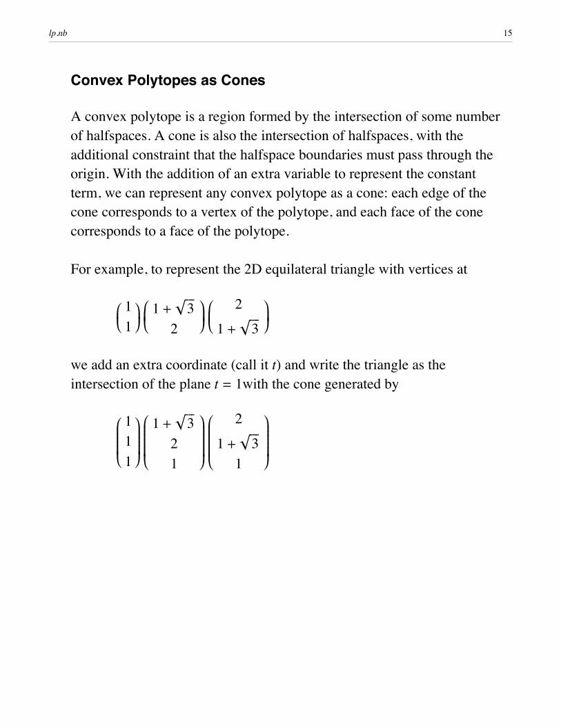
Convex Polytopes as Cones

A convex polytope is a region formed by the intersection of some number of halfspaces. A cone is also the intersection of halfspaces, with the additional constraint that the halfspace boundaries must pass through the origin. With the addition of an extra variable to represent the constant term, we can represent any convex polytope as a cone: each edge of the cone corresponds to a vertex of the polytope, and each face of the cone corresponds to a face of the polytope.

For example, to represent the 2D equilateral triangle with vertices at

ikjj

11y{zz ikjjj 1 +

è!!!32

y{zzz ikjjj

2

1 +è!!!3

y{zzz

we add an extra coordinate (call it t) and write the triangle as the intersection of the plane t = 1with the cone generated by

i

k

jjjjjjj

111

y

{

zzzzzzz i

k

jjjjjjjj

1 +è!!!3

21

y

{

zzzzzzzz i

k

jjjjjjjj

2

1 +è!!!3

1

y

{

zzzzzzzz

lp.nb 15

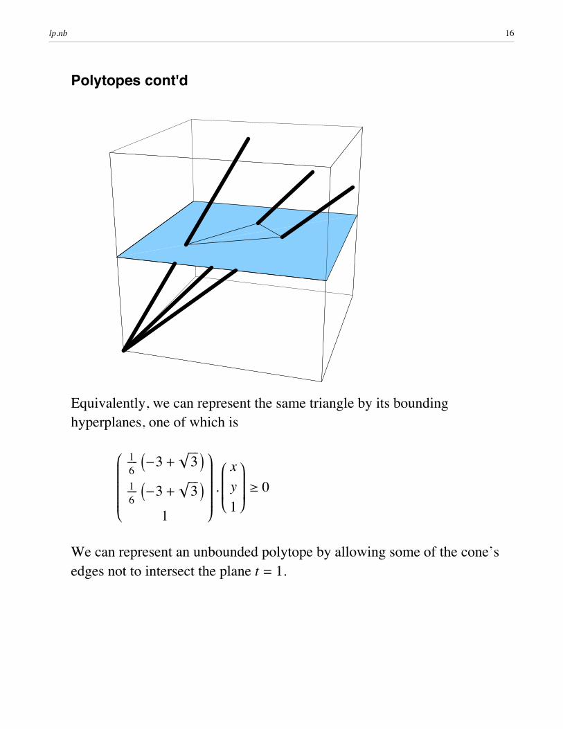
Polytopes cont'd

Equivalently, we can represent the same triangle by its bounding hyperplanes, one of which is

i

k

jjjjjjjjjjj

1ÅÅÅÅÅ6I-3 +

è!!!3 M1ÅÅÅÅÅ6I-3 +

è!!!3 M

1

y

{

zzzzzzzzzzz.i

k

jjjjjjj

xy1

y

{

zzzzzzz ¥ 0

We can represent an unbounded polytope by allowing some of the cone’s edges not to intersect the plane t = 1.

lp.nb 16

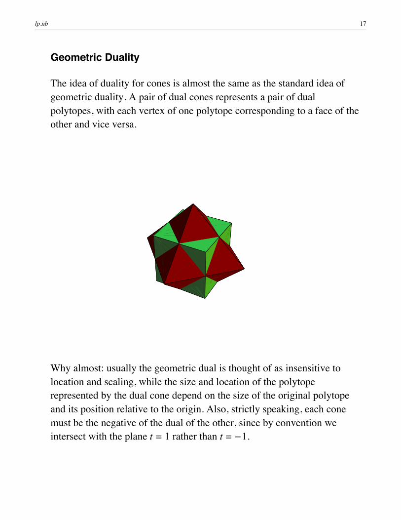
Geometric Duality

The idea of duality for cones is almost the same as the standard idea of geometric duality. A pair of dual cones represents a pair of dual polytopes, with each vertex of one polytope corresponding to a face of the other and vice versa.

Why almost: usually the geometric dual is thought of as insensitive to location and scaling, while the size and location of the polytope represented by the dual cone depend on the size of the original polytope and its position relative to the origin. Also, strictly speaking, each cone must be the negative of the dual of the other, since by convention we intersect with the plane t = 1 rather than t = -1.

lp.nb 17

The Lagrange Multiplier Theorem

We can now state the Lagrange multiplier theorem in its most general form, which tells how to minimize a function over an arbitrary convex polytope N x + c § 0.

Lagrange multiplier theorem: The problem of finding x to

minimize f HxLsubject to N x + c § 0

is equivalent to the problem of finding

arg minx maxpe—n+ LHx, pL

where the Lagrangian L is defined as

LHx, pL = f HxL + pT HN x + cL

for a vector of Lagrange multipliers p.

The Lagrange multiplier theorem uses properties of convex cones and duality to transform our original problem (involving an arbitrary polytope) to a problem which mentions only the very simple cone —n+. (—n+ is simple for two reasons: it is axis-parallel, and it is self-dual.)

The trade-offs are that we have introduced extra variables and that we are now looking for a saddle point rather than a minimum.

lp.nb 18

Linear Programming Duality

If f HxL is a linear function (say f ' x) then the minimization problem is a linear program.

The Lagrangian is f ' x+ p' HN x + cL or, rearranging terms, H f ' + p' NL x + p' c.

The latter is the Lagrangian for a new linear program (called the dual program):

maximize p' csubject to N ' p + f = 0 p ¥ 0

Since x was unrestricted in the original, or primal, program, it becomes a vector of Lagrange multipliers for an equality constraint in the dual program.

Note we minimize over x but maximize over p. (But changing § to ¥ changes p to -p.)

lp.nb 19

Duality cont'd

Even though the primal and dual Lagrangians are the same, the primal and dual programs are not (quite) the same problem: in one, we want minp maxx L, in the other we want maxx minp L.

It is a theorem (due to von Neumann) that these two values are the same (and so any x, p which achieves one also achieves the other).

For nonlinear optimization problems, infp supx L and supx infp L are not necessarily the same. The difference between the two is called a duality gap.

lp.nb 20

Complementary Slackness

If x, p is a saddle point of L, pT HN x + cL § 0 (else LHx, 2 pL > LHx, pL).

Similarly, pT HN x + cL ¥ 0 (else LIx, 1ÅÅÅÅÅ2

pM > LHx, pL).

So, pT HN x + cL = 0 (the complementary slackness condition).

Since, in general, N x + c will be zero in at most n coordinates, the remaining m - n components of p must be 0. (In fact, barring degeneracy, the constrained optimum will be at a vertex of the feasible region, so N x + c will be zero in exactly n coordinates and p will have exactly n nonzeros.)

lp.nb 21

Prices

Suppose x, p are a saddle point of f ' x + p' HN x + cL. How much does an increase of d in fi change the value of the optimum?

The value of the optimum increases by at least d xi, since the same x will still be feasible (although perhaps not optimal).

Similarly, a decrease of d in ci decreases the optimum by at least d pi.

For this reason, dual variables are sometimes called shadow prices.

lp.nb 22

Log-barrier Methods

Commercial linear-programming solvers today use variants of the logarithmic barrier method, a descendent of an algorithm introduced in the 1980s by N. Karmarkar.

Karmarkar's was the second polynomial-time algorithm to be discovered for linear programming, and the first practical one. (Khachiyan's ellipsoid algorithm was the first, but in practice simplex seems to beat it.)

We want to find a saddle point of L = f ' x + p' HN x + cL with the constraint p ¥ 0. Since even this simple constraint is inconvenient, consider what happens if we add an extra barrier term:

Lm = f ' x + p' HN x + cL - m ln pi

The effect of the barrier term is to make Lm Ø ! as pi Ø 0, so that we can ignore the constraints on p and work entirely with a smooth function. The relative importance of the barrier term is controlled by the barrier parameter m > 0.

lp.nb 23

Log-Barrier cont'd

For fixed x and m, Lm is strictly convex, and so has a unique minimum. For fixed p and m, Lm is linear.

For each m, Lm defines a saddle-point problem in x, p. For large m, the problem is very smooth (and easy to solve); as m Ø 0, Lm Ø L and Hx*, p*Lm Ø x* , p*.

Since Lm is smooth, we can find the saddle point by setting “Lm = 0 or

N ' p + f = 0N x + c = m p-1

where p-1 means the componentwise inverse of p.

The basic idea of the log-barrier method is to start with a large m and follow the trajectory of solutions as m Ø 0. This trajectory is called the central path.

lp.nb 24

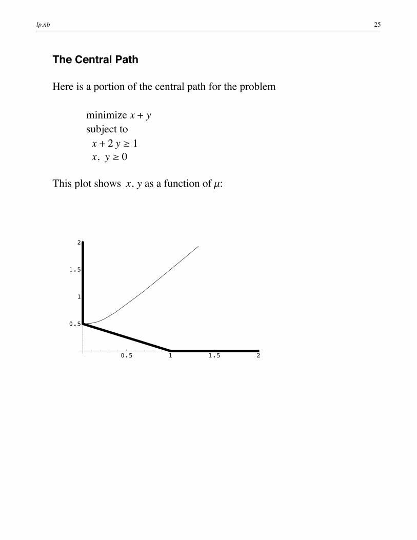
The Central Path

Here is a portion of the central path for the problem

minimize x+ ysubject to x + 2 y ¥ 1x, y ¥ 0

This plot shows x, y as a function of m:

0.5 1 1.5 2

0.5

1

1.5

2

lp.nb 25

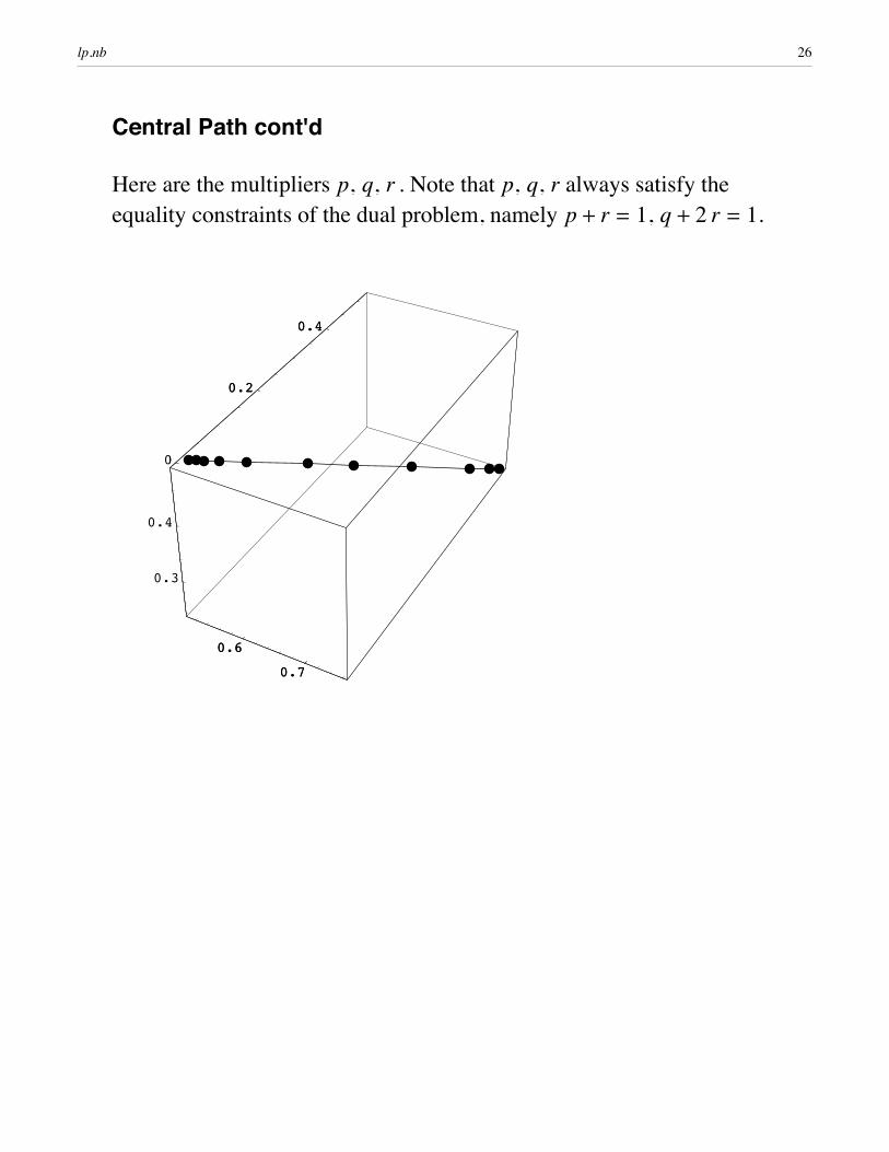
Central Path cont'd

Here are the multipliers p, q, r . Note that p, q, r always satisfy the equality constraints of the dual problem, namely p + r = 1, q + 2 r = 1.

0.6

0.7

0

0.2

0.4

0.3

0.4

0.6

0.7

0

0.2

0.4

lp.nb 26

Following the Central Path

Again, the optimality conditions are “Lm = 0 or

N ' p + f = 0N x + c = m p-1

If we start with a guess at x, p for a particular m, we can refine the guess with one or more steps of Newton's method.

After we're satisfied with the accuracy, we can decrease m and start again (using our previous solution as an initial guess). (One could—although we won't—derive bounds on how close we need to be to the solution before we can safely decrease m.)

With the appropriate (nonobvious!) strategy for reducing m as much as possible after each Newton step, we have a polynomial time algorithm. (In practice, we never use a provably-polynomial strategy since all the known ones are very conservative.)

lp.nb 27