linear regression and correlation analysis. regression analysis regression analysis attempts to...
TRANSCRIPT
Linear Regression and
Correlation Analysis
Regression Analysis
Regression Analysis attempts to determine the strength of the relationship between one dependent variable (usually denoted by Y) and a series of other changing variables (known as independent variables).
Regression AnalysisRegression Analysis is used to:
Predict the value of a dependent variable based on the value of at least one independent variable
Explain the impact of changes in an independent variable on the dependent variable
Dependent Variable: The variable we wish to explain
Independent Variable: The variable used to explain the dependent variable
Regression Analysis• One of the two variables (X, Y), say X is an
independent variable/ controlled variable/ ordinary variable, Y is random Variable
• Relationship between X and Y is described by a linear function
• Dependence of Y on X or Regression of Y on X
• Dependence of Blood Pressure Y on X
• Regression of gain of weight Y on food X
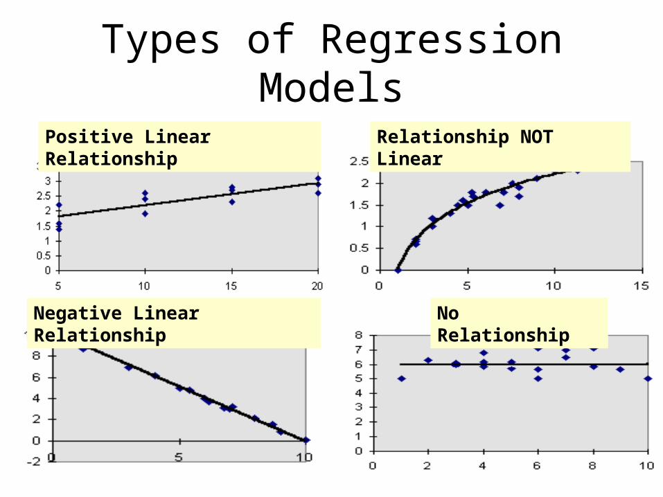
Types of Regression Models
Positive Linear Relationship
Negative Linear Relationship
Relationship NOT Linear
No Relationship
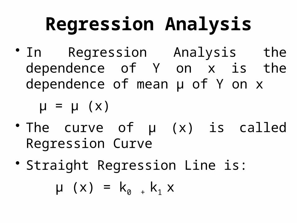
Regression Analysis• In Regression Analysis the dependence of Y
on x is the dependence of mean µ of Y on x
µ = µ (x)
• The curve of µ (x) is called Regression Curve
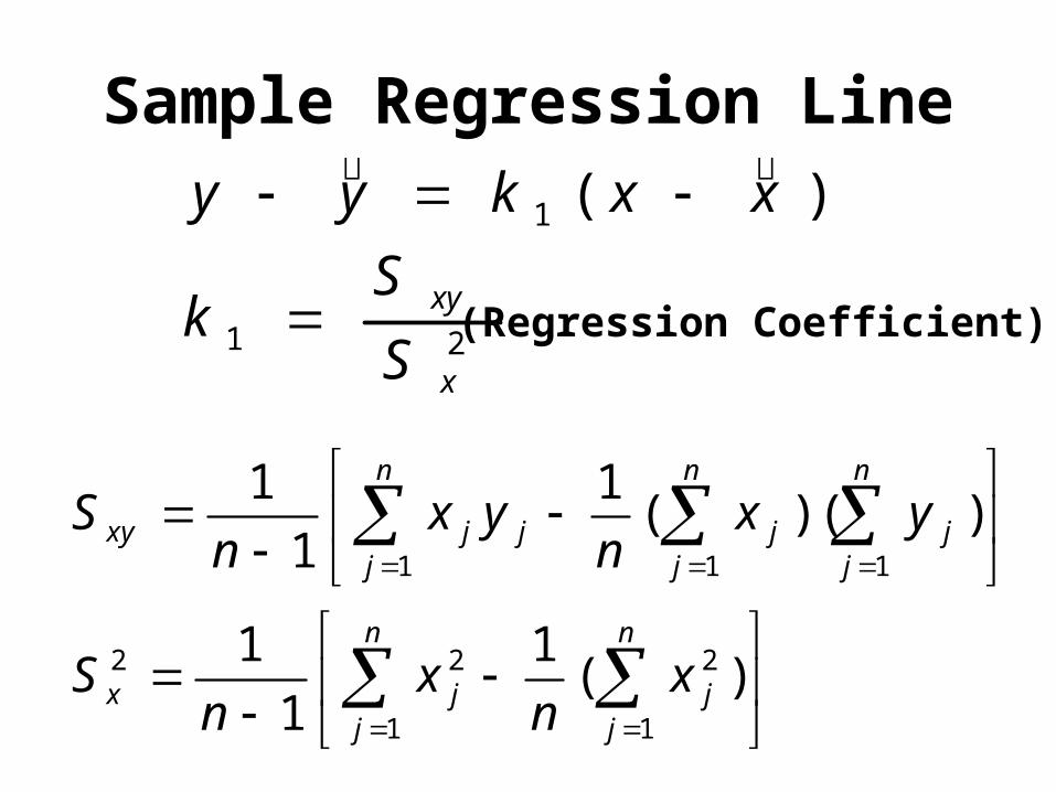
• Straight Regression Line is:
µ (x) = k0 + k1 x
xkk)( 10 x
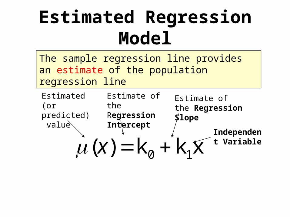
The sample regression line provides an estimate of the population regression line
Estimated Regression Model
Estimate of the Regression Intercept
Estimate of the Regression Slope
Estimated (or predicted) value
Independent Variable
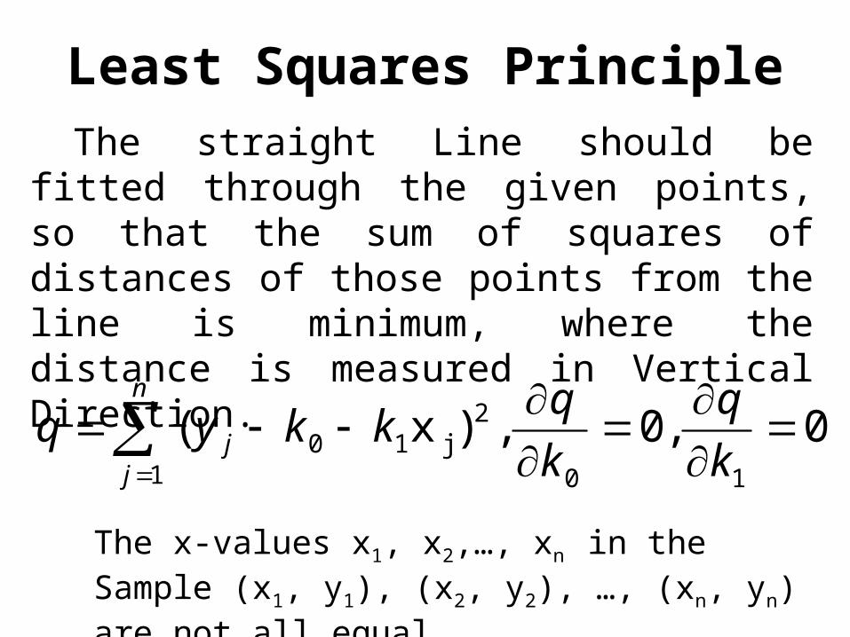
Least Squares PrincipleThe straight Line should be fitted through
the given points, so that the sum of squares of distances of those points from the line is minimum, where the distance is measured in Vertical Direction.
0,0,)x(10
2j10
1
k
q
k
qkkyq
n
jj
The x-values x1, x2,…, xn in the Sample (x1, y1), (x2, y2), …, (xn, yn) are not all equal.

Sample Regression Line
21
21
21
1
)...(1
)...(1
)(
x
xy
n
n
S
Sk
yyyn
y
xxxn
x
xxkyy
�
�
��
(Regression Coefficient)
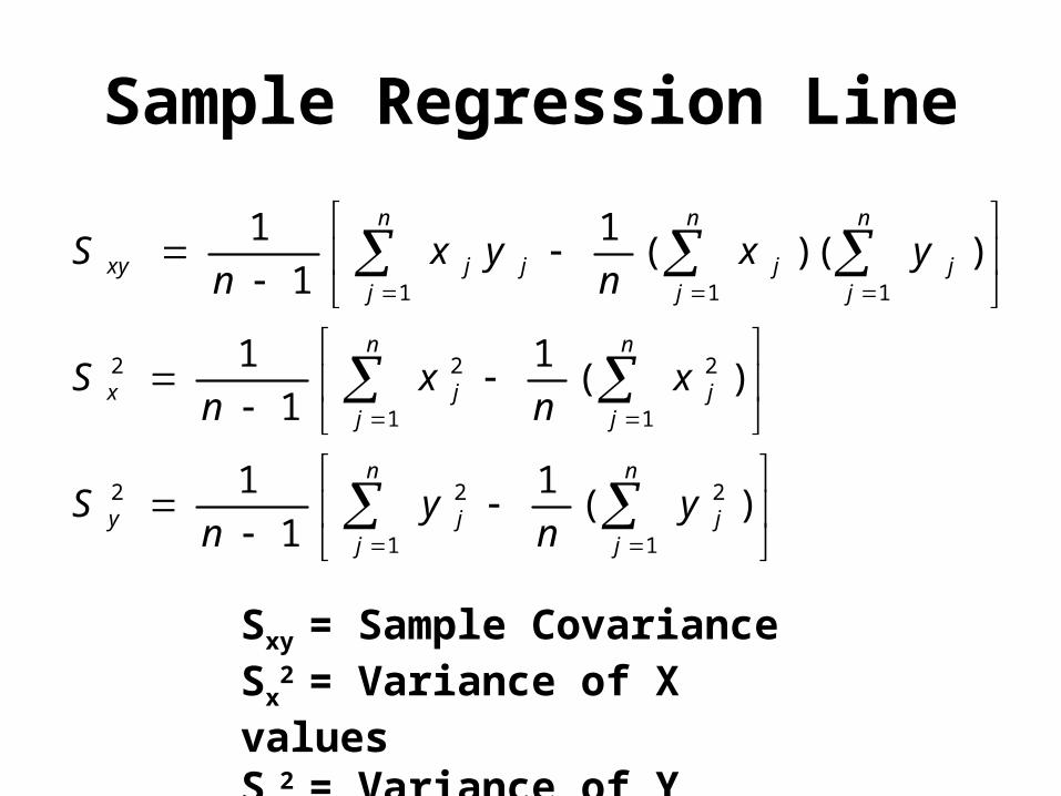
Sample Regression Line
n
j
n
jjjy
n
j
n
jjjx
n
j
n
j
n
jjjjjxy
yn
yn
S
xn
xn
S
yxn
yxn
S
1 1
222
1 1
222
1 1 1
)(1
1
1
)(1
1
1
))((1
1
1
Sxy = Sample CovarianceSx
2 = Variance of X valuesSy
2 = Variance of Y values
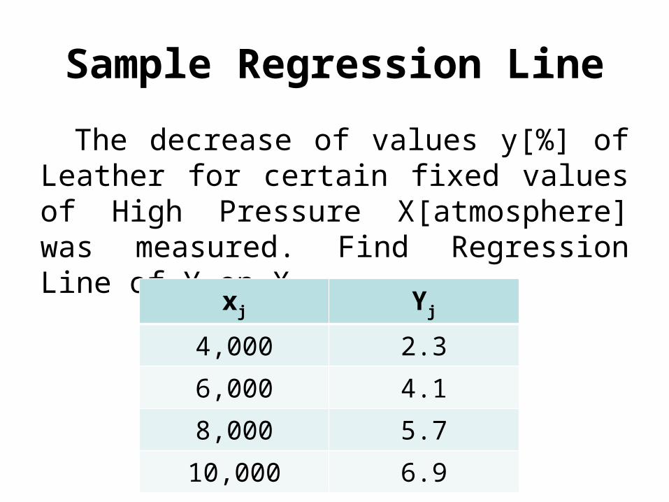
Sample Regression Line
The decrease of values y[%] of Leather for certain fixed values of High Pressure X[atmosphere] was measured. Find Regression Line of Y on X.
xj Yj
4,000 2.36,000 4.18,000 5.7
10,000 6.9
Sample Regression Line
21
1 )(
x
xy
S
Sk
xxkyy
��
(Regression Coefficient)
n
j
n
jjjx
n
j
n
j
n
jjjjjxy
xn
xn
S
yxn
yxn
S
1 1
222
1 1 1
)(1
1
1
))((1
1
1
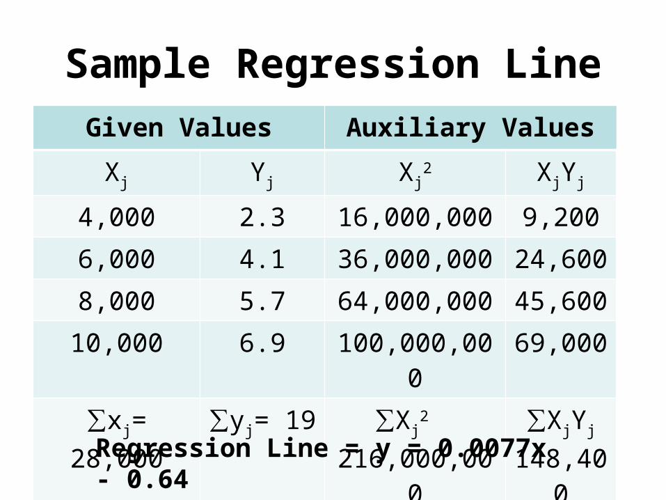
Sample Regression LineGiven Values Auxiliary Values
Xj Yj Xj2 XjYj
4,000 2.3 16,000,000 9,2006,000 4.1 36,000,000 24,6008,000 5.7 64,000,000 45,600
10,000 6.9 100,000,000 69,000∑xj= 28,000 ∑yj= 19 ∑Xj
2 216,000,000
∑XjYj
148,400
Regression Line = y = 0.0077x - 0.64
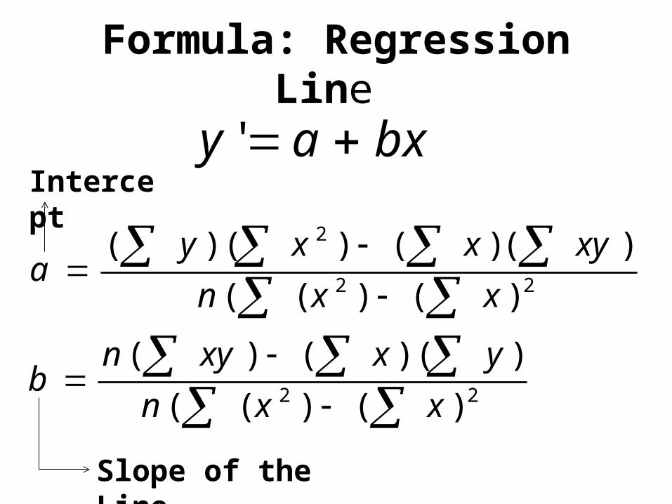
Formula: Regression Line
22
22
2
)()((
))(()(
)()((
)()())((
xxn
yxxynb
xxn
xyxxya
bxay 'Intercept
Slope of the Line
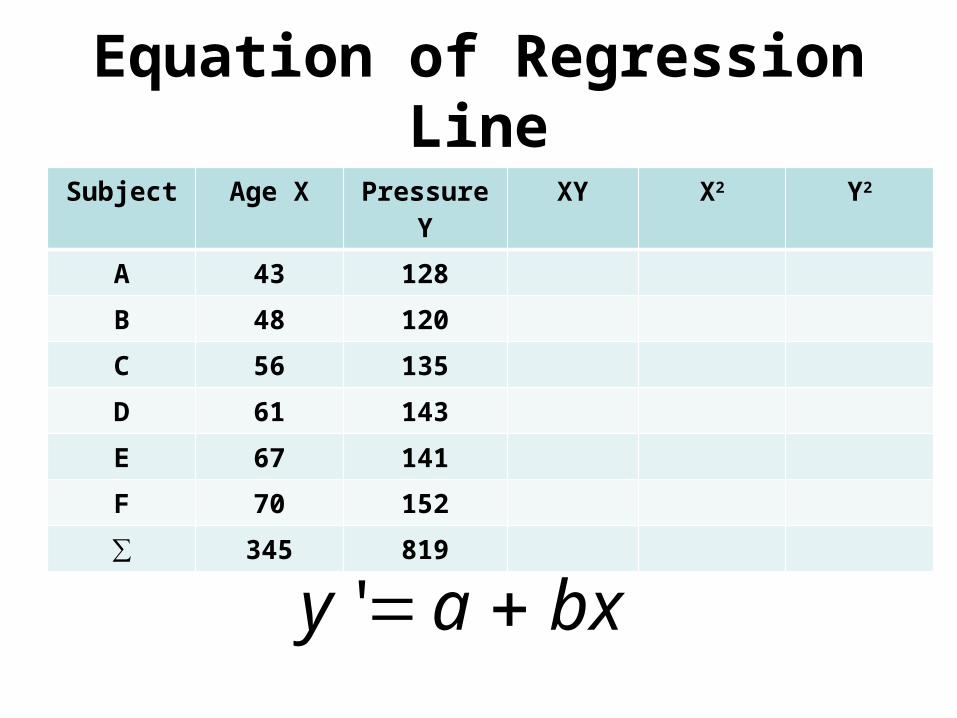
Equation of Regression Line
Subject Age X Pressure Y XY X2 Y2
A 43 128
B 48 120
C 56 135
D 61 143
E 67 141
F 70 152
∑ 345 819
bxay '
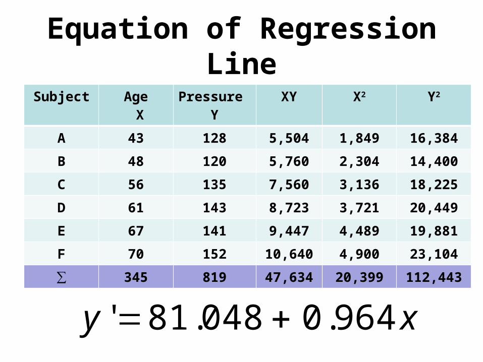
Equation of Regression Line
Subject Age X
Pressure Y
XY X2 Y2
A 43 128 5,504 1,849 16,384
B 48 120 5,760 2,304 14,400
C 56 135 7,560 3,136 18,225
D 61 143 8,723 3,721 20,449
E 67 141 9,447 4,489 19,881
F 70 152 10,640 4,900 23,104
∑ 345 819 47,634 20,399 112,443
xy 964.0048.81'
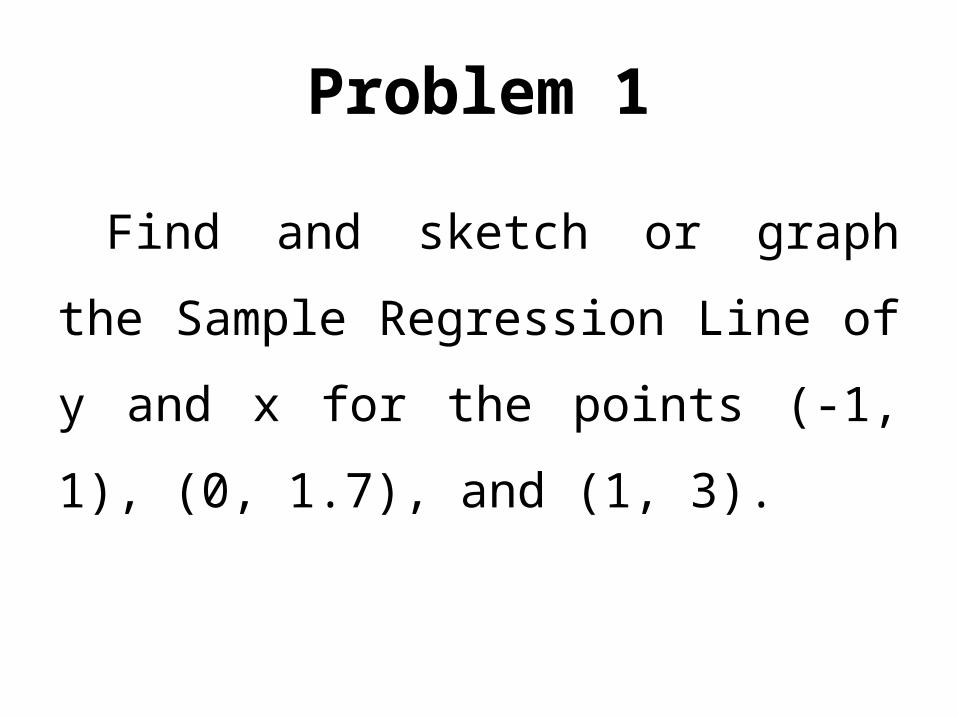
Problem 1
Find and sketch or graph the Sample
Regression Line of y and x for the
points (-1, 1), (0, 1.7), and (1, 3).
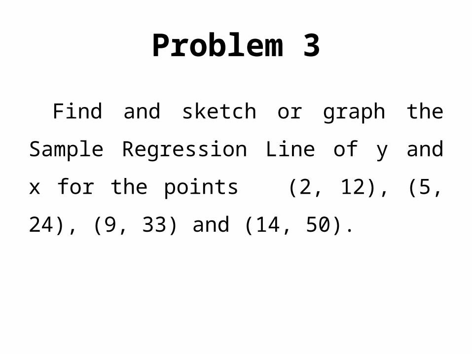
Problem 3
Find and sketch or graph the Sample
Regression Line of y and x for the points
(2, 12), (5, 24), (9, 33) and (14, 50).
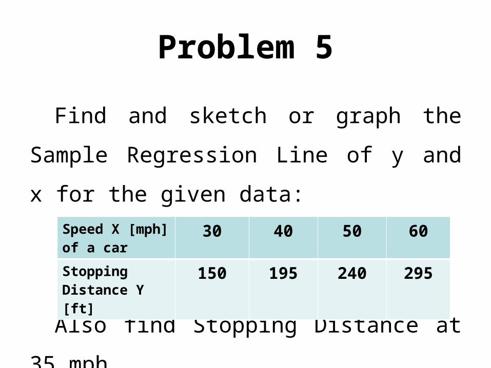
Problem 5
Find and sketch or graph the Sample
Regression Line of y and x for the given
data:
Also find Stopping Distance at 35 mph.
Speed X [mph] of a car
30 40 50 60
Stopping Distance Y [ft]
150 195 240 295
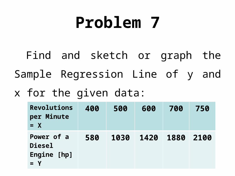
Problem 7
Find and sketch or graph the Sample
Regression Line of y and x for the given
data:Revolutions per Minute = X
400 500 600 700 750
Power of a Diesel Engine [hp] = Y
580 1030 1420 1880 2100
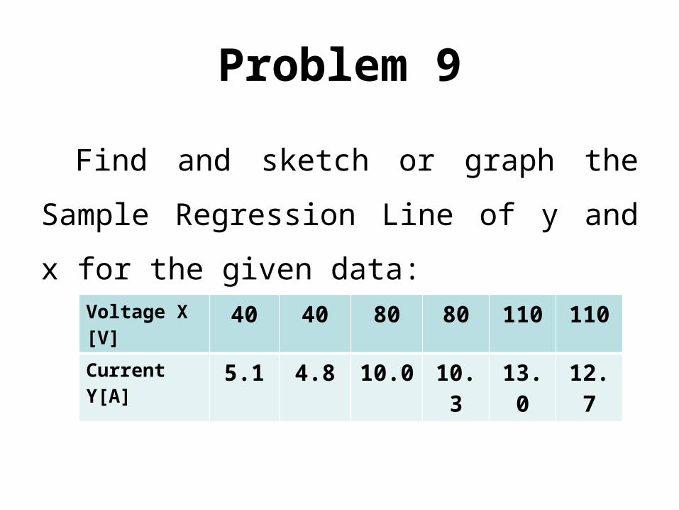
Problem 9
Find and sketch or graph the Sample
Regression Line of y and x for the given
data:Voltage X [V] 40 40 80 80 110 110Current Y[A]
5.1 4.8 10.0 10.3 13.0 12.7
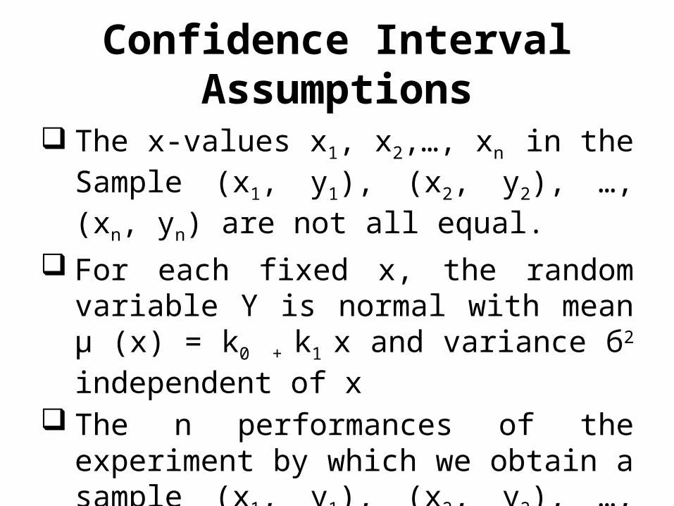
Confidence IntervalAssumptions
The x-values x1, x2,…, xn in the Sample (x1, y1), (x2, y2), …, (xn, yn) are not all equal.
For each fixed x, the random variable Y is normal with mean µ (x) = k0 + k1 x and variance б2 independent of x
The n performances of the experiment by which we obtain a sample (x1, y1), (x2, y2), …, (xn, yn) are independent.
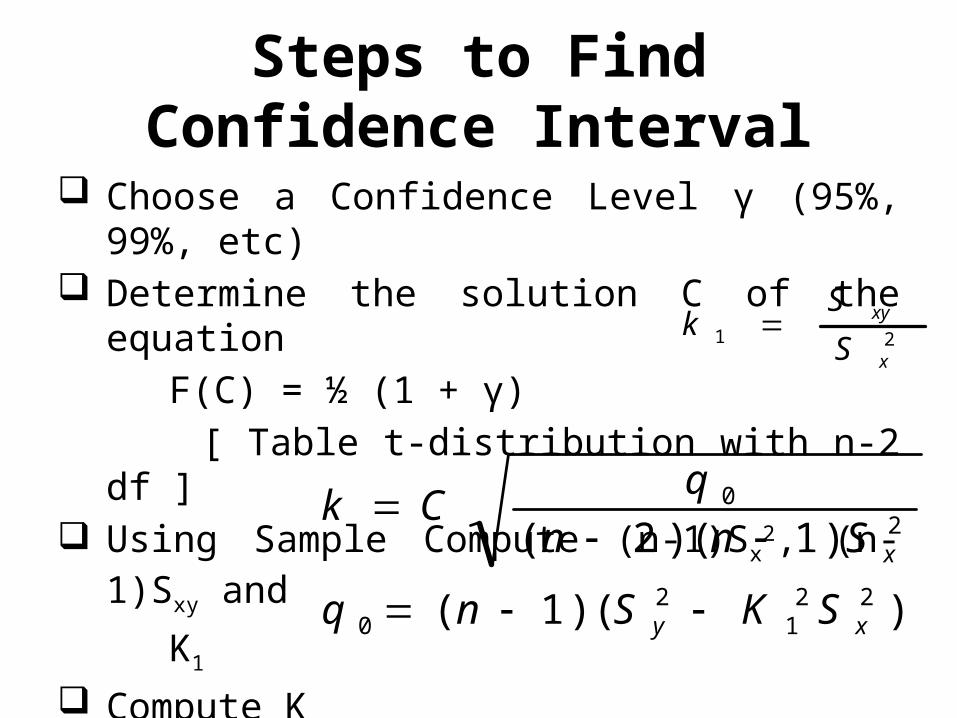
Steps to FindConfidence Interval
Choose a Confidence Level γ (95%, 99%, etc) Determine the solution C of the equation
F(C) = ½ (1 + γ)
[ Table t-distribution with n-2 df ] Using Sample Compute (n-1)Sx
2, (n-1)Sxy and
K1
Compute K
Confidence Interval (K1 – K ≤ K1 ≤ K1 + K)
))(1(
)1)(2(22
12
0
20
xy
x
SKSnq
Snn
qCk
21x
xy
S
Sk
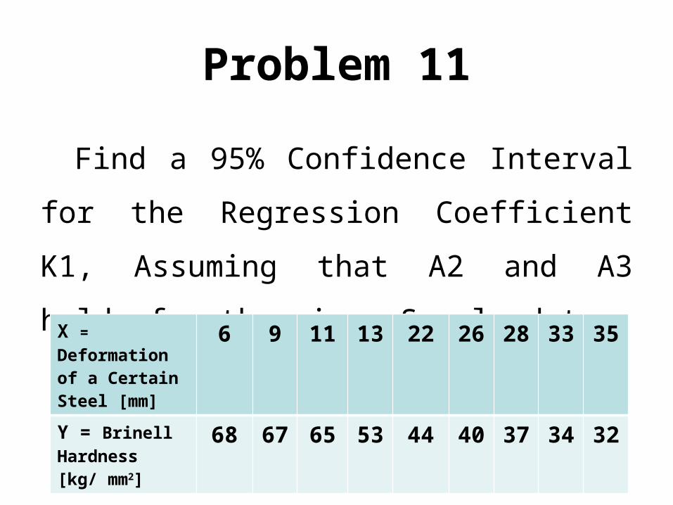
Problem 11
Find a 95% Confidence Interval for the
Regression Coefficient K1, Assuming that
A2 and A3 hold, for the given Sample data:
X = Deformation of a Certain Steel [mm]
6 9 11 13 22 26 28 33 35
Y = Brinell Hardness [kg/ mm2]
68 67 65 53 44 40 37 34 32
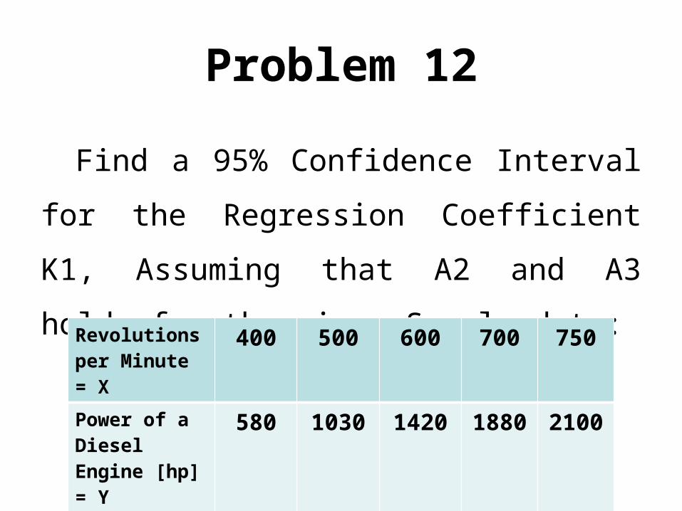
Problem 12
Find a 95% Confidence Interval for the
Regression Coefficient K1, Assuming that
A2 and A3 hold, for the given Sample data:
Revolutions per Minute = X
400 500 600 700 750
Power of a Diesel Engine [hp] = Y
580 1030 1420 1880 2100
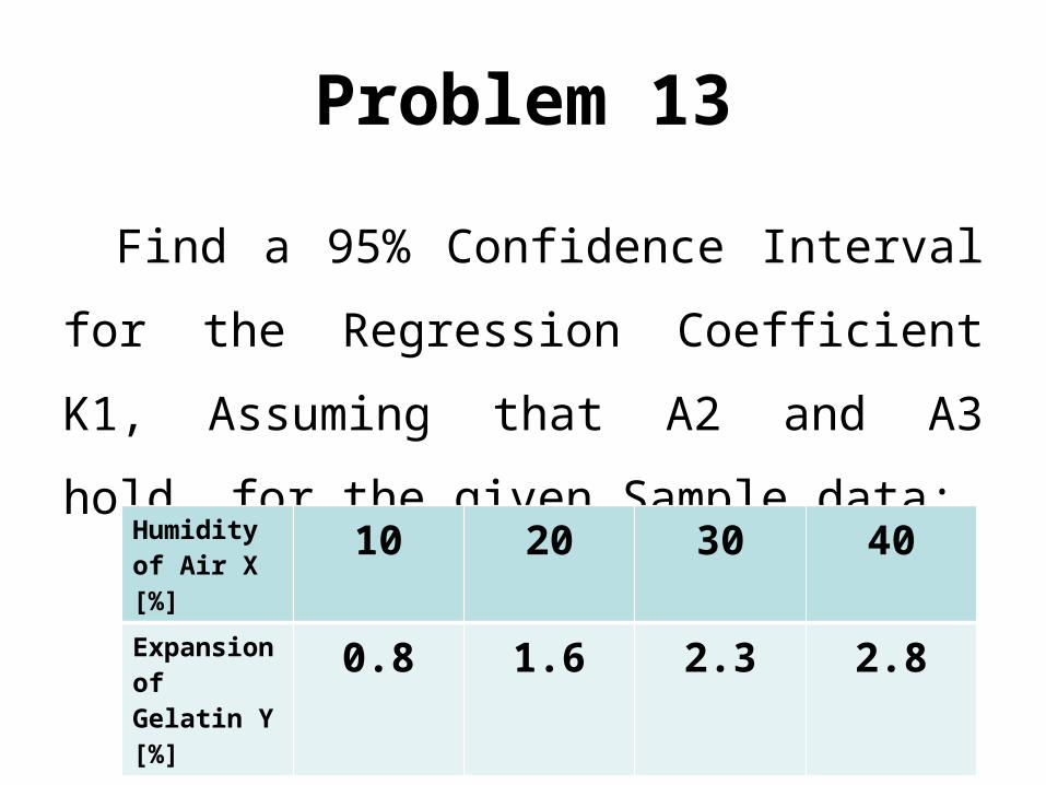
Problem 13
Find a 95% Confidence Interval for the
Regression Coefficient K1, Assuming that
A2 and A3 hold, for the given Sample data:
Humidity of Air X [%]
10 20 30 40Expansion of Gelatin Y [%]
0.8 1.6 2.3 2.8

Correlation Analysis
• Both variables (X, Y) are random variables– Grades X and Y of students in Math and
Physics
– Hardness X of steel plates in the centre and hardness Y near the edges of the plates
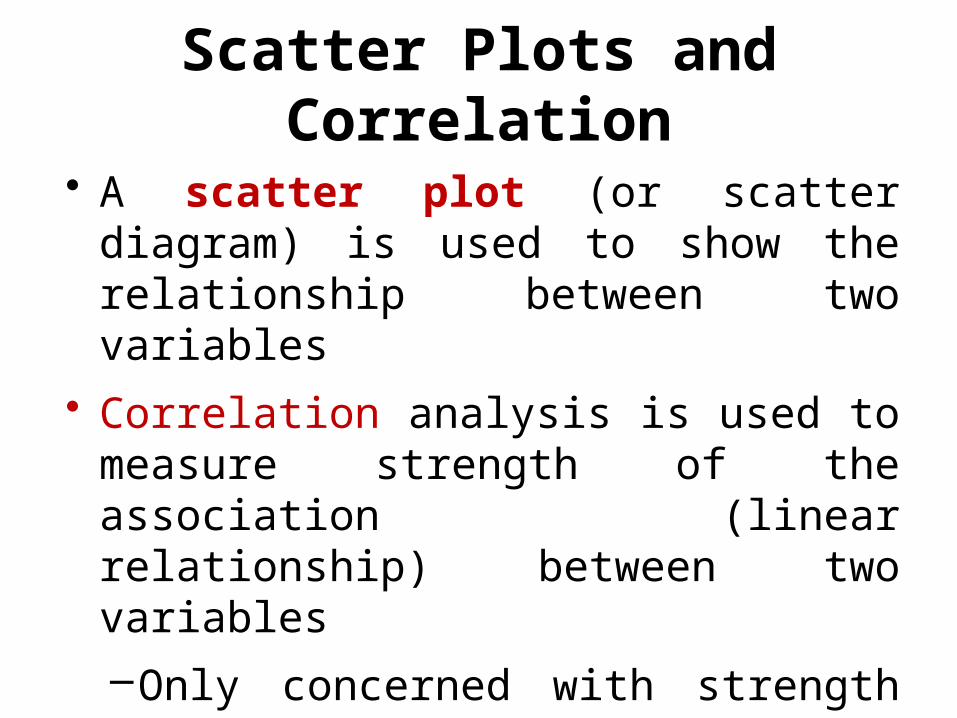
Scatter Plots and Correlation
• A scatter plot (or scatter diagram) is used to show the relationship between two variables
• Correlation analysis is used to measure strength of the association (linear relationship) between two variables
–Only concerned with strength of the relationship
–No causal effect is implied
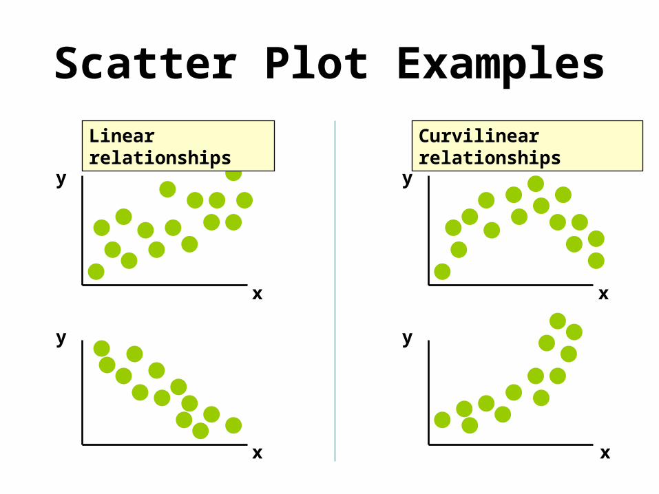
Scatter Plot Examples
y
x
y
x
y
y
x
x
Linear relationships Curvilinear relationships
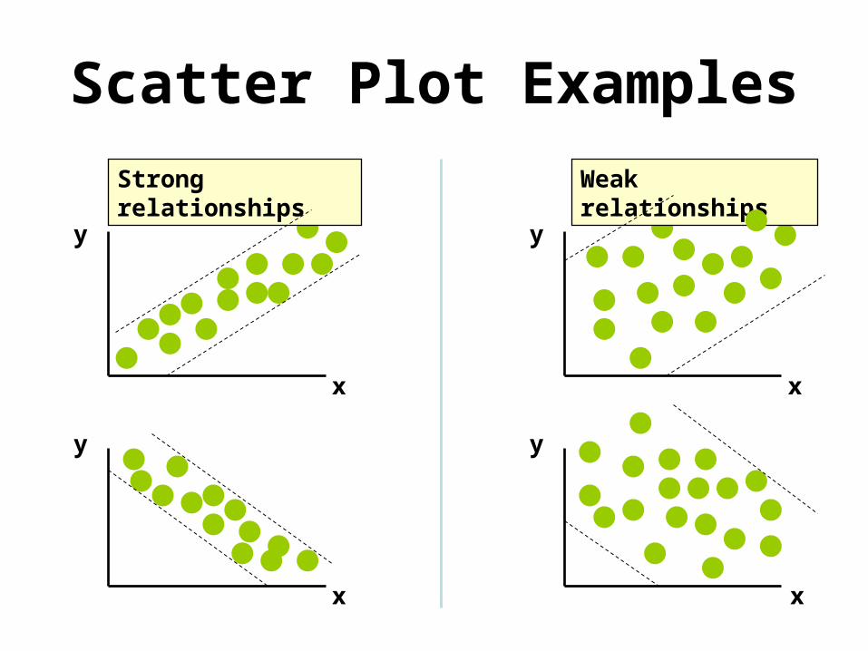
Scatter Plot Examples
y
x
y
x
y
y
x
x
Strong relationships Weak relationships
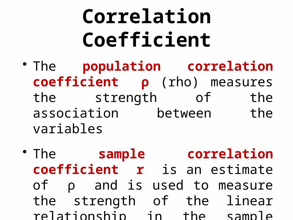
Correlation Coefficient
• The population correlation coefficient ρ (rho) measures the strength of the association between the variables
• The sample correlation coefficient r is an estimate of ρ and is used to measure the strength of the linear relationship in the sample observations
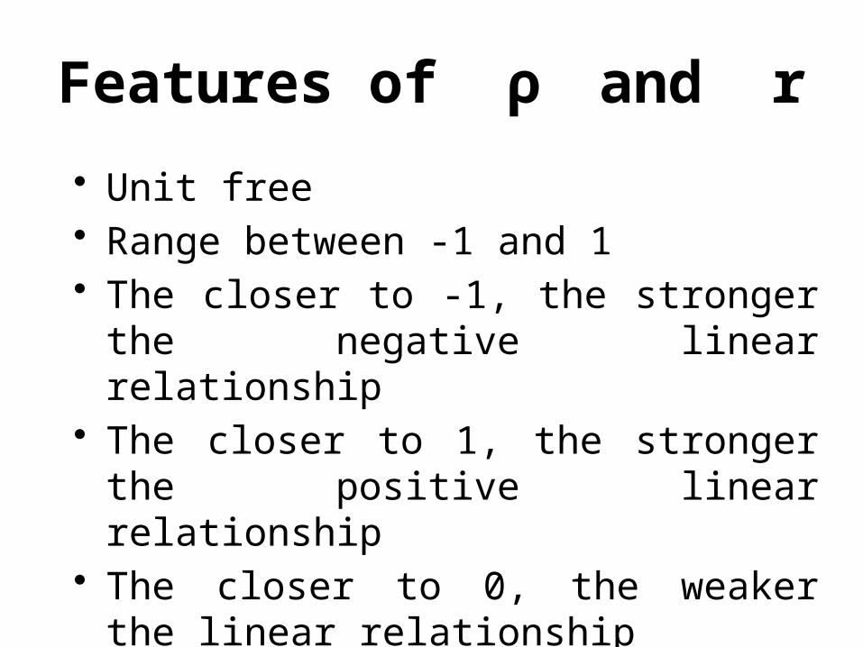
Features of ρ and r
• Unit free• Range between -1 and 1• The closer to -1, the stronger the negative
linear relationship• The closer to 1, the stronger the positive
linear relationship• The closer to 0, the weaker the linear
relationship
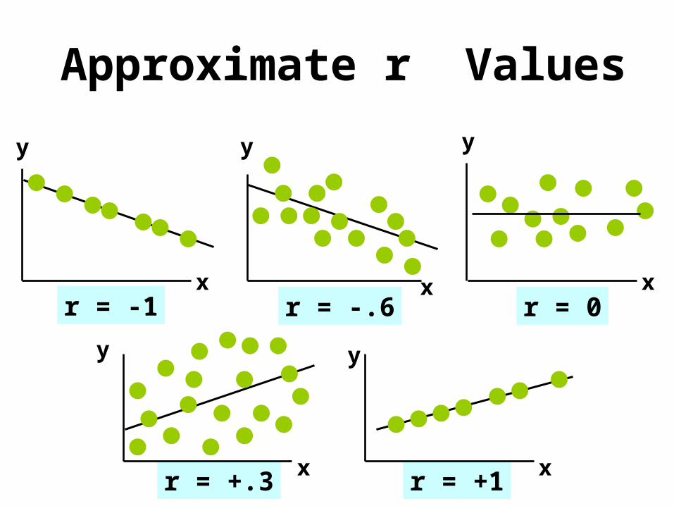
r = +.3 r = +1
Approximate r Values
y
x
y
x
y
x
y
x
y
x
r = -1 r = -.6 r = 0
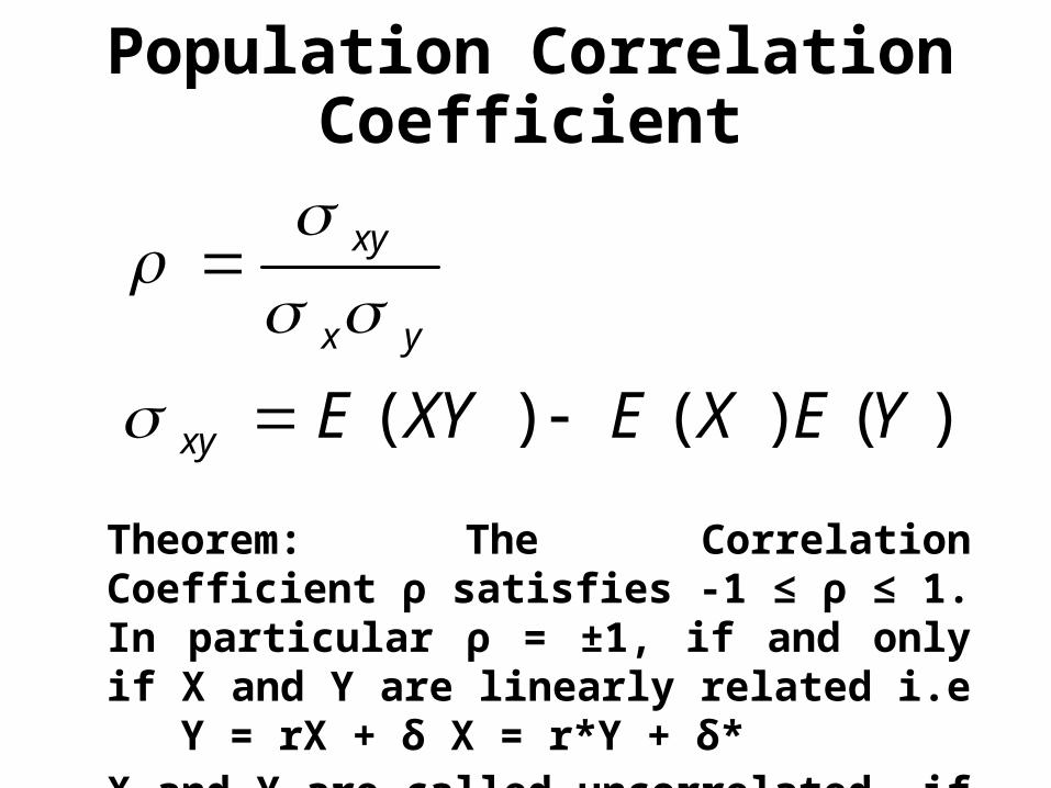
Population Correlation Coefficient
Theorem: The Correlation Coefficient ρ satisfies -1 ≤ ρ ≤ 1. In particular ρ = ±1, if and only if X and Y are linearly related i.e Y = rX + δ X = r*Y + δ*
X and Y are called uncorrelated, if ρ = 0.
)()()( YEXEXYExy
yx
xy
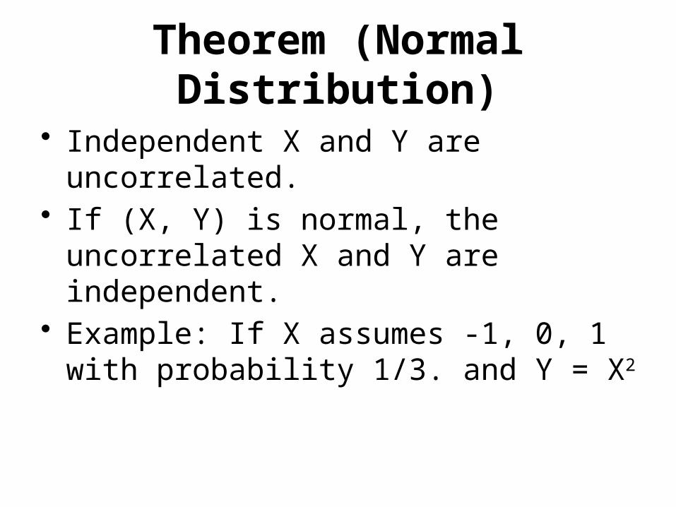
Theorem (Normal Distribution)
• Independent X and Y are uncorrelated.• If (X, Y) is normal, the uncorrelated X and
Y are independent.• Example: If X assumes -1, 0, 1 with
probability 1/3. and Y = X2
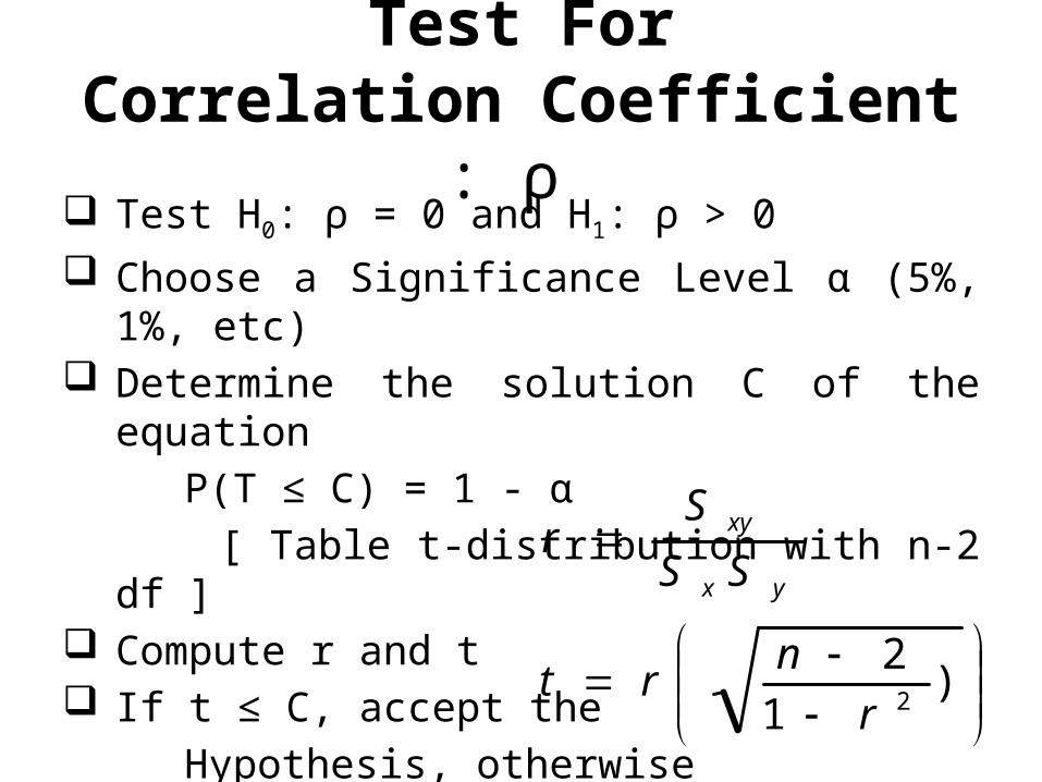
Test ForCorrelation Coefficient : ρ
Test H0: ρ = 0 and H1: ρ > 0
Choose a Significance Level α (5%, 1%, etc) Determine the solution C of the equation
P(T ≤ C) = 1 - α
[ Table t-distribution with n-2 df ] Compute r and t If t ≤ C, accept the
Hypothesis, otherwise
reject the Hypothesis.
)1
22r
nrt
SS
Sr
yx
xy
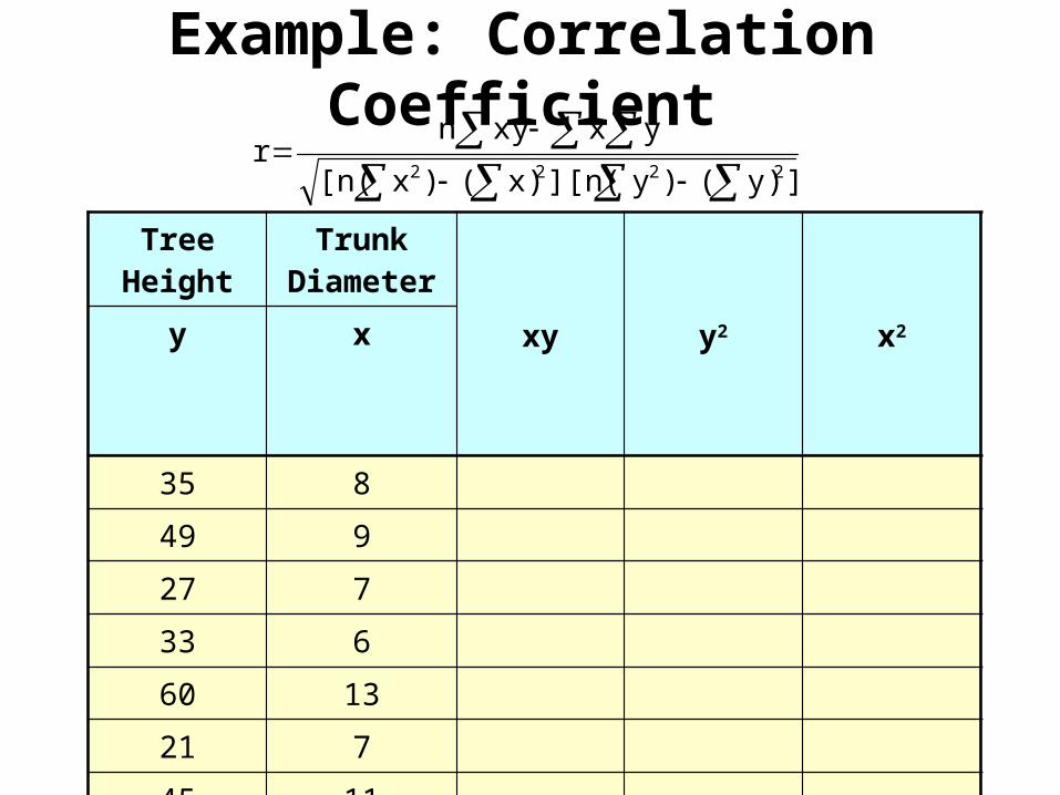
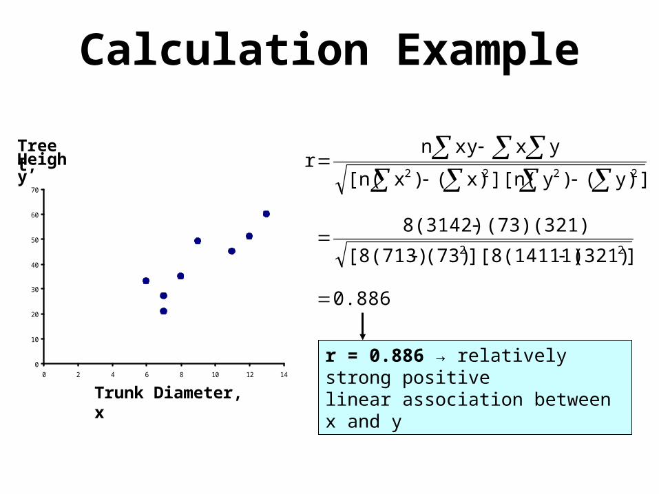
Example: Correlation Coefficient
Tree Height
Trunk Diameter
xy y2 x2y x
35 8
49 9
27 7
33 6
60 13
21 7
45 11
51 12
=321 =73
]y)()y][n(x)()x[n(
yxxynr
2222
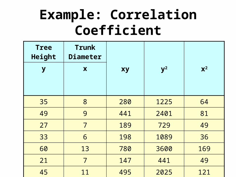
Example: Correlation Coefficient
Tree Height
Trunk Diameter
xy y2 x2y x
35 8 280 1225 64
49 9 441 2401 81
27 7 189 729 49
33 6 198 1089 36
60 13 780 3600 169
21 7 147 441 49
45 11 495 2025 121
51 12 612 2601 144
=321 =73 =3142 =14111 =713
0
10
20
30
40
50
60
70
0 2 4 6 8 10 12 14
0.886
](321)][8(14111)(73)[8(713)
(73)(321)8(3142)
]y)()y][n(x)()x[n(
yxxynr
22
2222
Trunk Diameter, x
TreeHeight, y
Calculation Example
r = 0.886 → relatively strong positive linear association between x and y
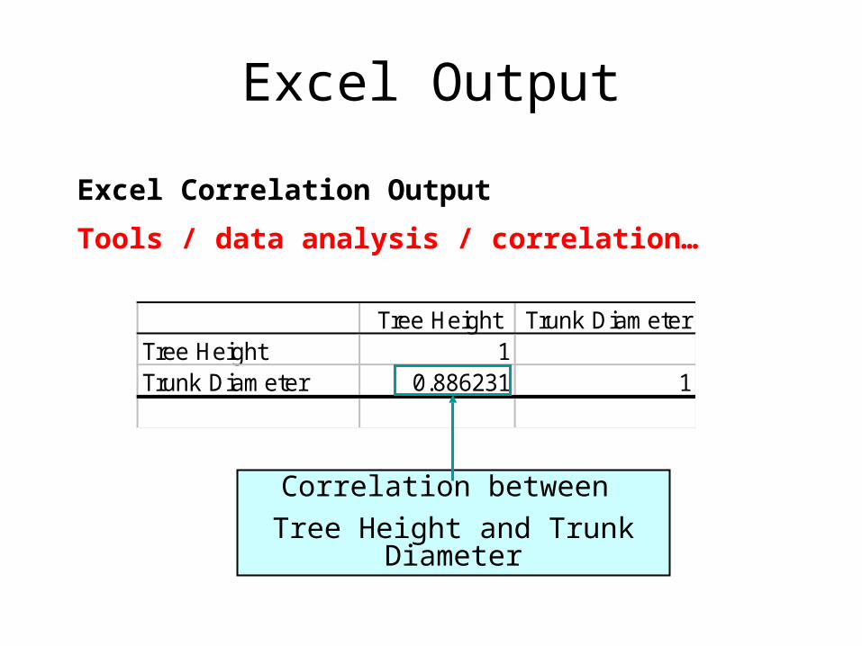
Excel Output
Tree Height Trunk DiameterTree Height 1Trunk Diameter 0.886231 1
Excel Correlation Output
Tools / data analysis / correlation…
Correlation between
Tree Height and Trunk Diameter
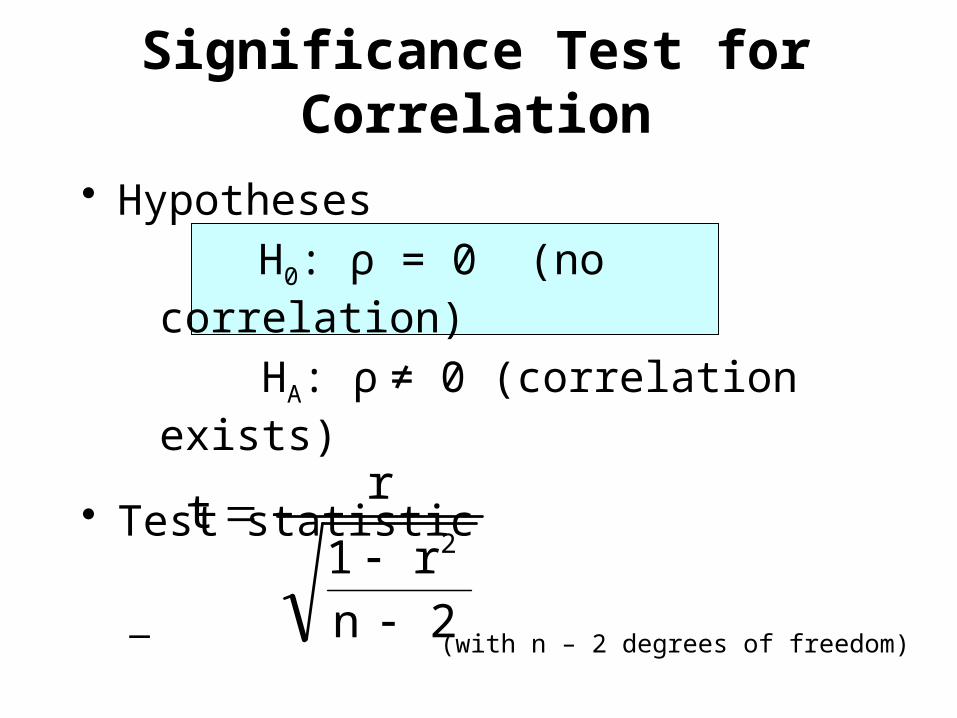
Significance Test for Correlation
• Hypotheses
H0: ρ = 0 (no correlation)
HA: ρ ≠ 0 (correlation exists)
• Test statistic
– (with n – 2 degrees of freedom)
2nr1
rt
2

Example: Produce Stores
Is there evidence of a linear relationship between tree height and trunk diameter at the .05 level of significance?
H0: ρ = 0 (No correlation)
H1: ρ ≠ 0 (correlation exists)
=.05 , df = 8 - 2 = 6
4.68
28.8861
.886
2nr1
rt
22
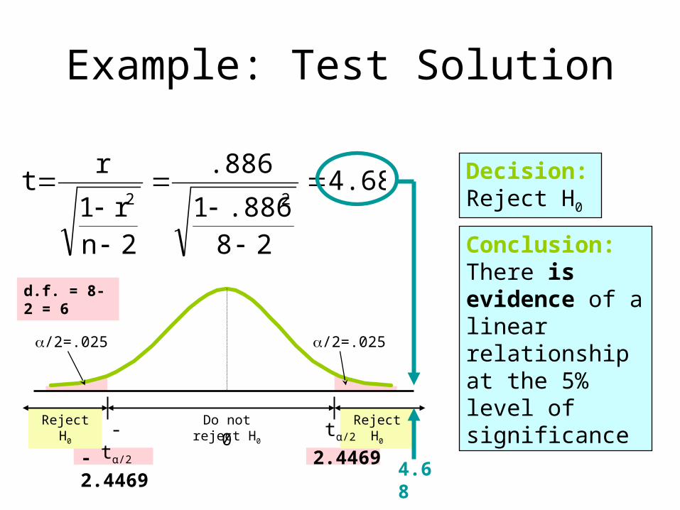
4.68
28.8861
.886
2nr1
rt
22
Example: Test Solution
Conclusion:There is evidence of a linear relationship at the 5% level of significance
Decision:Reject H0
Reject H0Reject H0
a/2=.025
-tα/2
Do not reject H0
0 tα/2
a/2=.025
-2.4469 2.44694.68
d.f. = 8-2 = 6

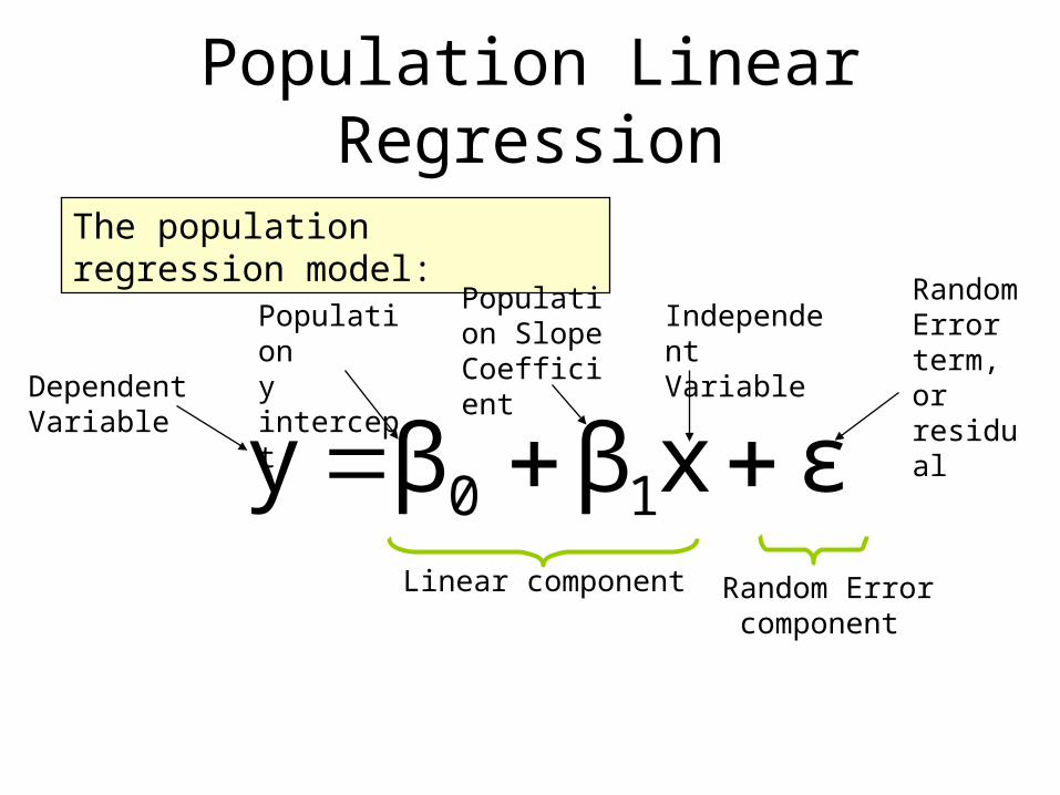
εxββy 10 Linear component
Population Linear Regression
The population regression model:
Population y intercept
Population SlopeCoefficient
Random Error term, or residualDependent
Variable
Independent Variable
Random Error component
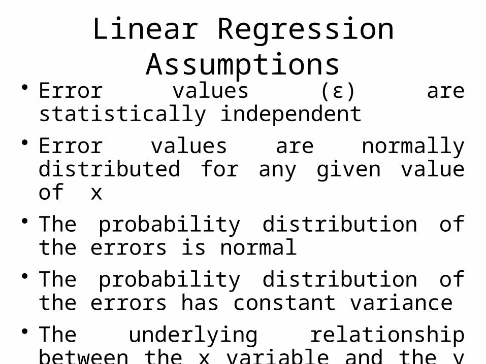
Linear Regression Assumptions• Error values (ε) are statistically independent• Error values are normally distributed for any
given value of x• The probability distribution of the errors is
normal• The probability distribution of the errors has
constant variance• The underlying relationship between the x
variable and the y variable is linear
Population Linear Regression(continued)
Random Error for this x value
y
x
Observed Value of y for xi
Predicted Value of y for xi
εxββy 10
xi
Slope = β1
Intercept = β0
εi
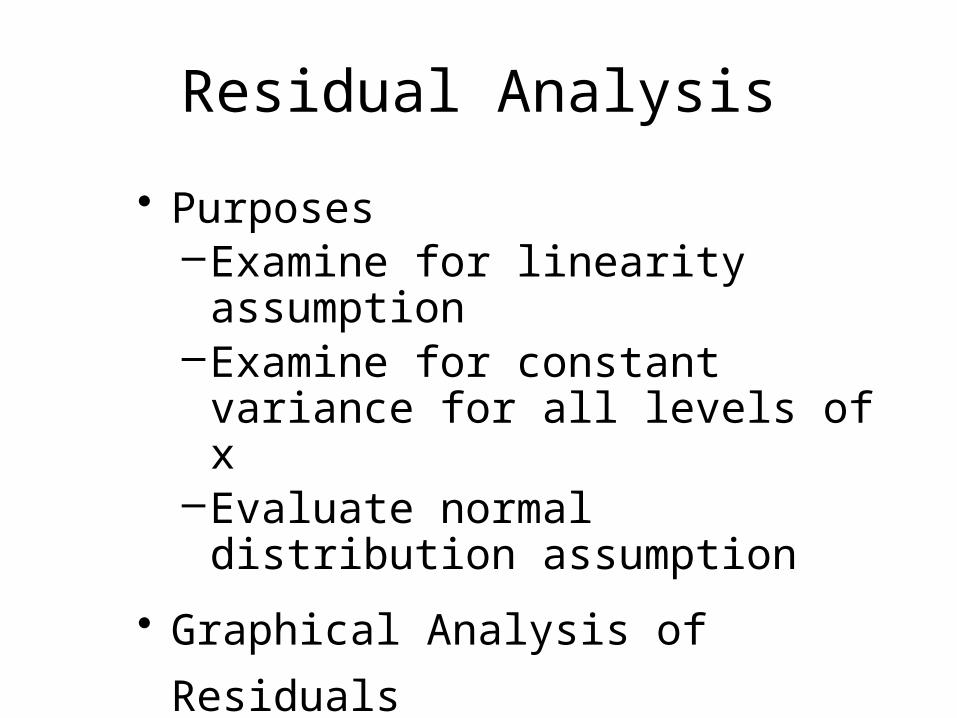
Residual Analysis
• Purposes–Examine for linearity assumption–Examine for constant variance for all
levels of x –Evaluate normal distribution
assumption
• Graphical Analysis of Residuals–Can plot residuals vs. x–Can create histogram of residuals to
check for normality
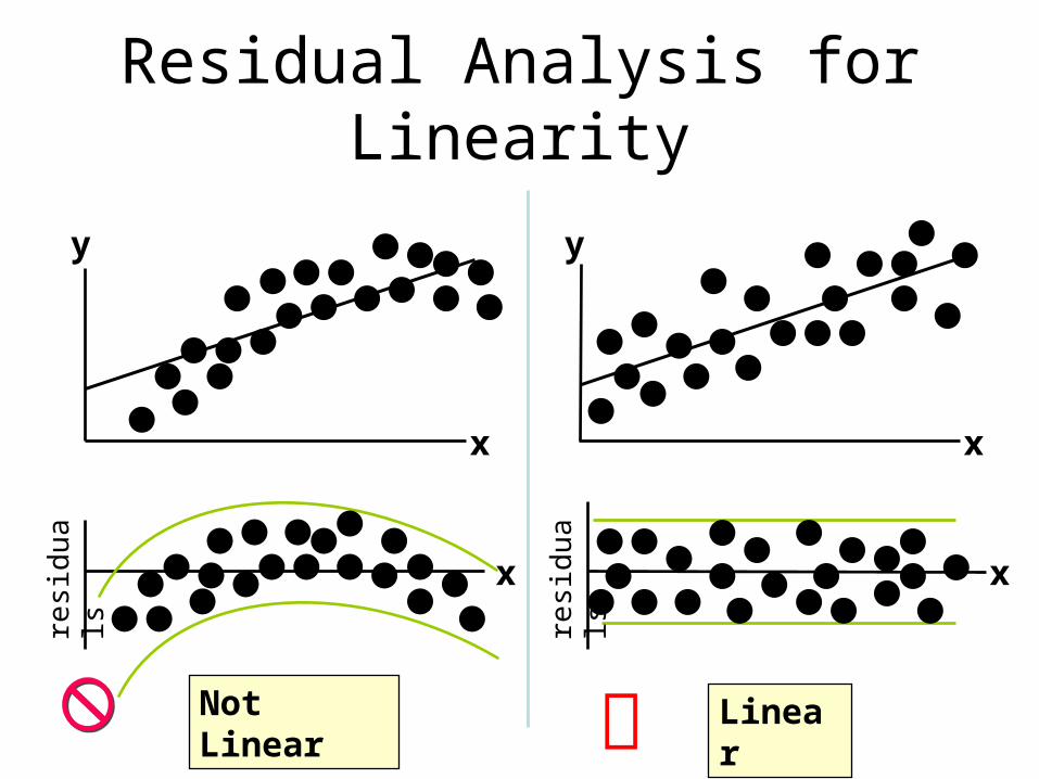
Residual Analysis for Linearity
Not Linear Linear
x
resi
dua
ls
x
y
x
y
x
resi
dua
ls
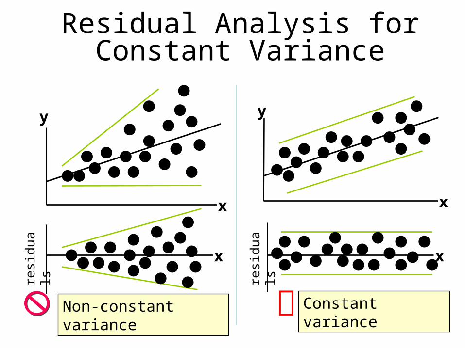
Residual Analysis for Constant Variance
Non-constant variance Constant variance
x x
y
x x
y
resi
dua
ls
resi
dua
ls
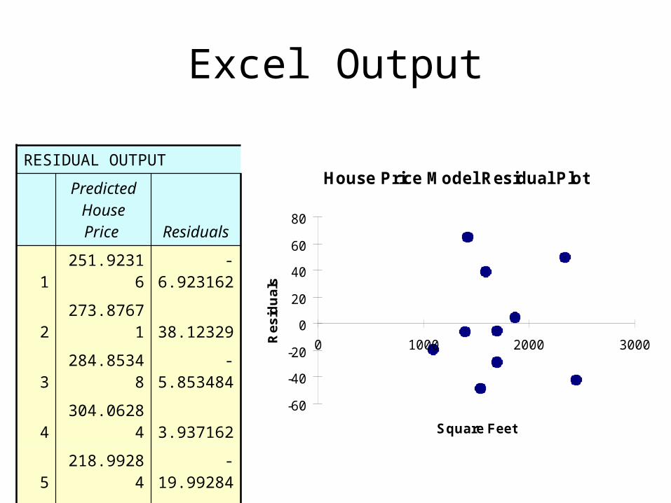
House Price Model Residual Plot
-60
-40
-20
0
20
40
60
80
0 1000 2000 3000
Square Feet
Re
sid
ua
ls
Excel Output
RESIDUAL OUTPUT
Predicted House Price Residuals
1 251.92316 -6.923162
2 273.87671 38.12329
3 284.85348 -5.853484
4 304.06284 3.937162
5 218.99284 -19.99284
6 268.38832 -49.38832
7 356.20251 48.79749
8 367.17929 -43.17929
9 254.6674 64.33264
10 284.85348 -29.85348
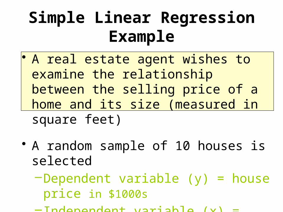
Simple Linear Regression Example
• A real estate agent wishes to examine the relationship between the selling price of a home and its size (measured in square feet)
• A random sample of 10 houses is selected–Dependent variable (y) = house price in
$1000s– Independent variable (x) = square feet
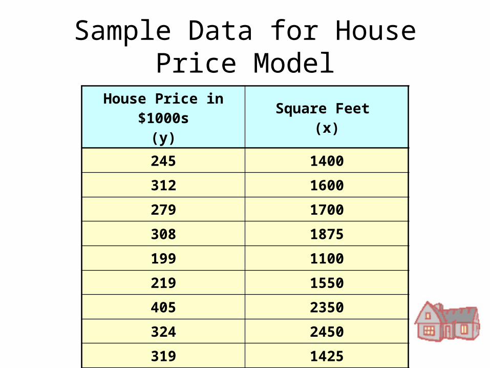
Sample Data for House Price Model
House Price in $1000s(y)
Square Feet (x)
245 1400
312 1600
279 1700
308 1875
199 1100
219 1550
405 2350
324 2450
319 1425
255 1700
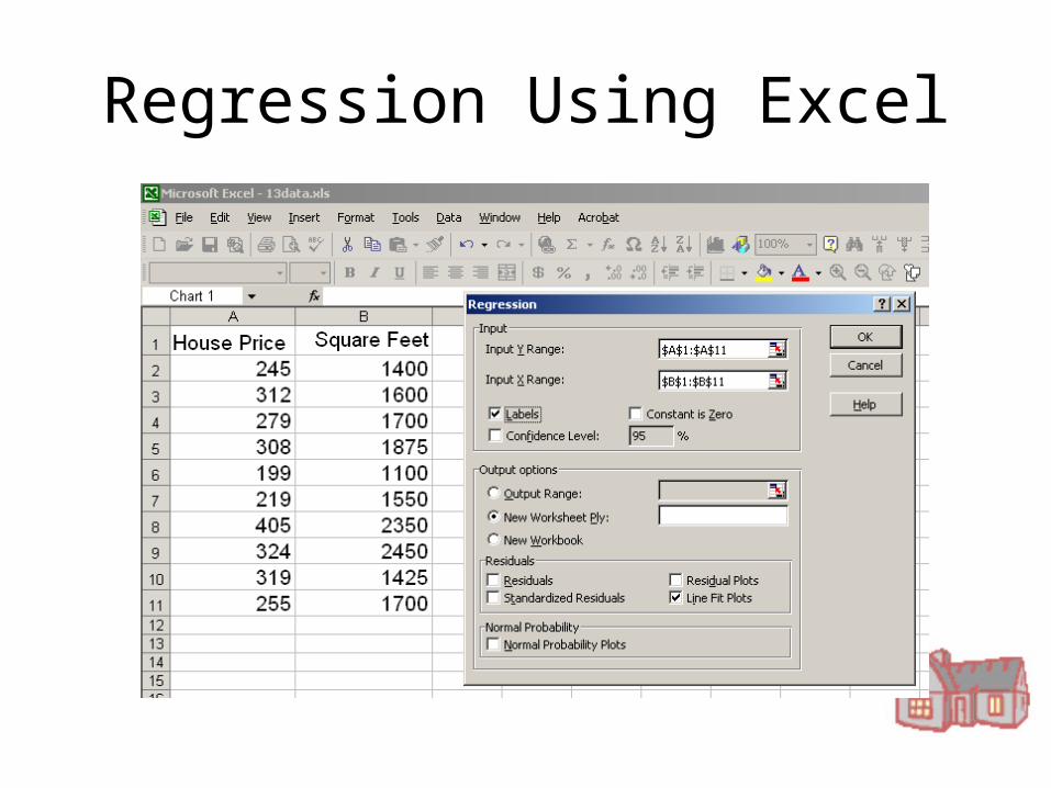
Regression Using Excel
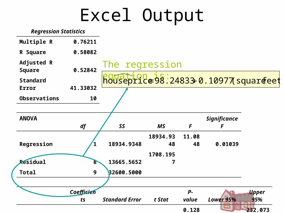
Excel OutputRegression Statistics
Multiple R 0.76211
R Square 0.58082
Adjusted R Square 0.52842
Standard Error 41.33032
Observations 10
ANOVA df SS MS F
Significance F
Regression 1 18934.934818934.934
811.084
8 0.01039
Residual 8 13665.5652 1708.1957
Total 9 32600.5000
Coefficien
ts Standard Error t StatP-
value Lower 95%Upper 95%
Intercept 98.24833 58.03348 1.692960.1289
2 -35.57720232.0738
6
Square Feet 0.10977 0.03297 3.329380.0103
9 0.03374 0.18580
The regression equation is:
feet) (square 0.10977 98.24833 price house
0
50
100
150
200
250
300
350
400
450
0 500 1000 1500 2000 2500 3000
Square Feet
Ho
use
Pri
ce (
$100
0s)
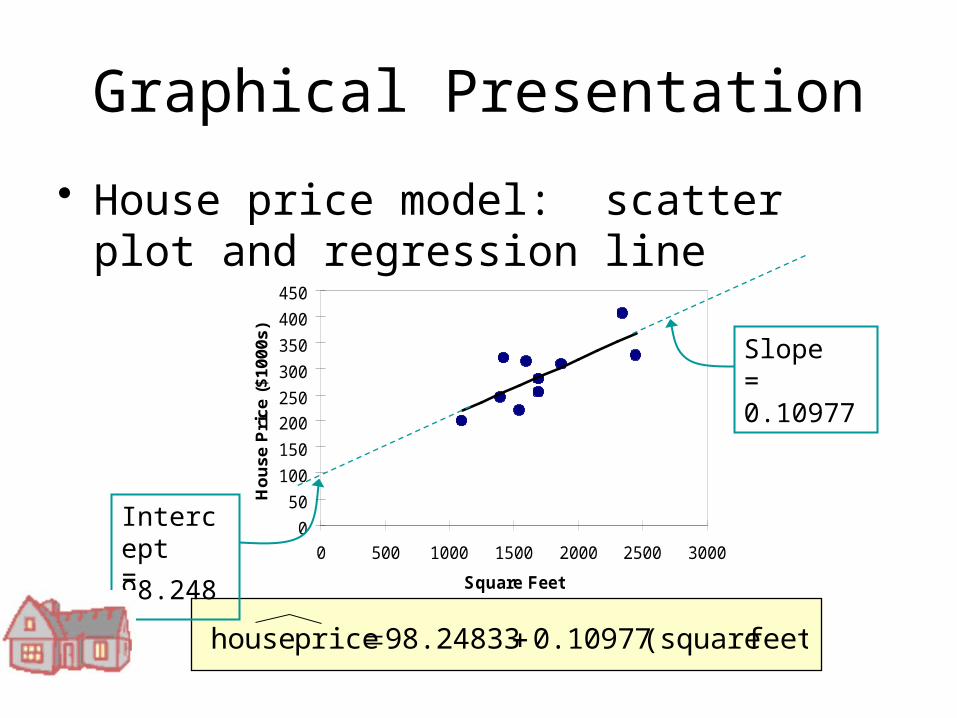
Graphical Presentation
• House price model: scatter plot and regression line
feet) (square 0.10977 98.24833 price house
Slope = 0.10977
Intercept = 98.248
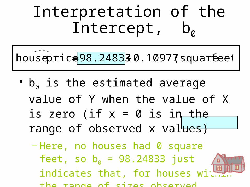
Interpretation of the Intercept, b0
• b0 is the estimated average value of Y
when the value of X is zero (if x = 0 is in the range of observed x values)
– Here, no houses had 0 square feet, so b0 =
98.24833 just indicates that, for houses within the range of sizes observed, $98,248.33 is the portion of the house price not explained by square feet
feet) (square 0.10977 98.24833 price house
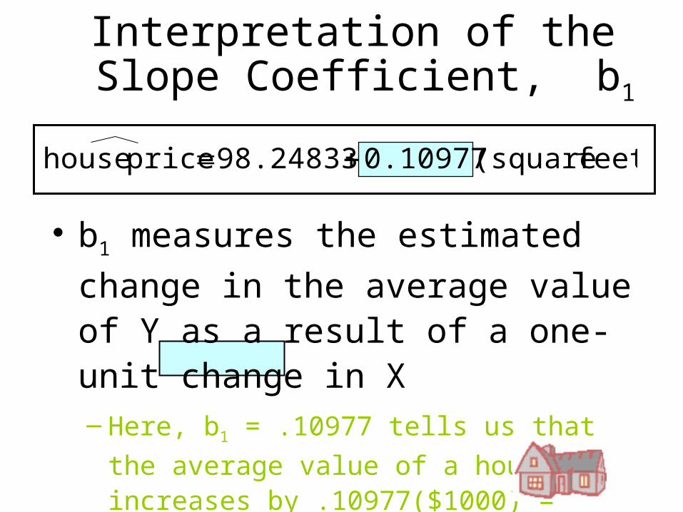
Interpretation of the Slope Coefficient, b1
• b1 measures the estimated change in
the average value of Y as a result of a one-unit change in X– Here, b1 = .10977 tells us that the average
value of a house increases by .10977($1000) = $109.77, on average, for each additional one square foot of size
feet) (square 0.10977 98.24833 price house
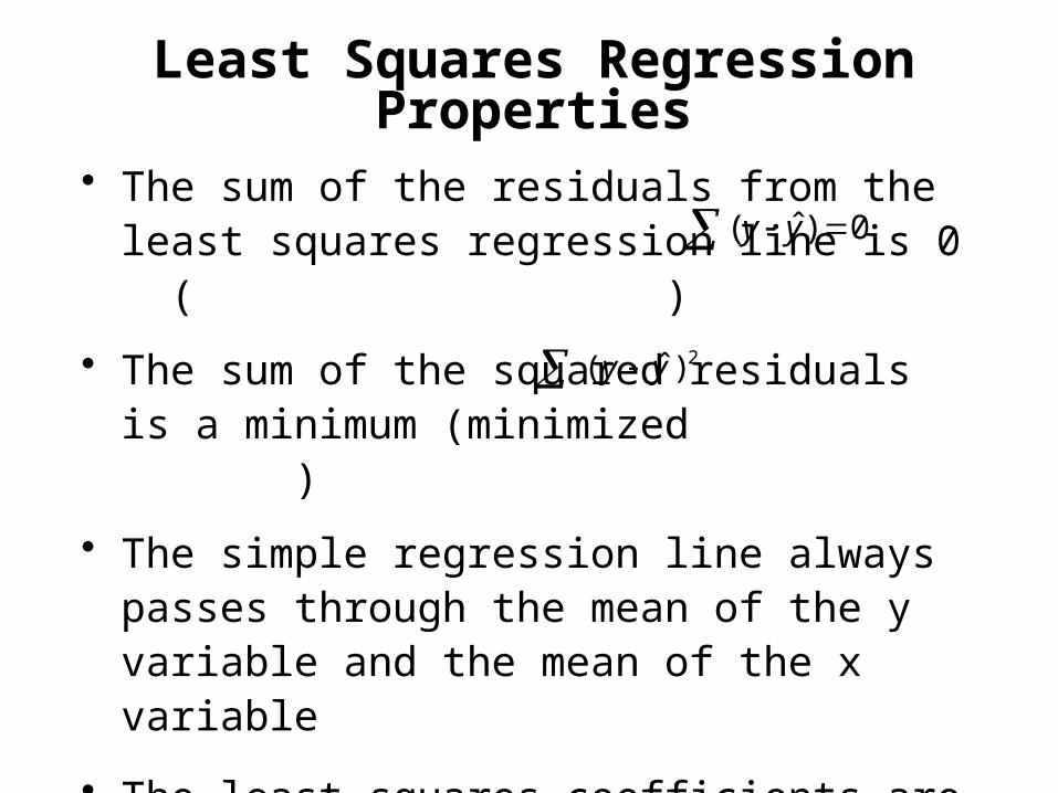
Least Squares Regression Properties
• The sum of the residuals from the least squares regression line is 0 ( )
• The sum of the squared residuals is a minimum (minimized )
• The simple regression line always passes through the mean of the y variable and the mean of the x variable
• The least squares coefficients are unbiased
estimates of β0 and β1
0)ˆ( yy
2)ˆ( yy
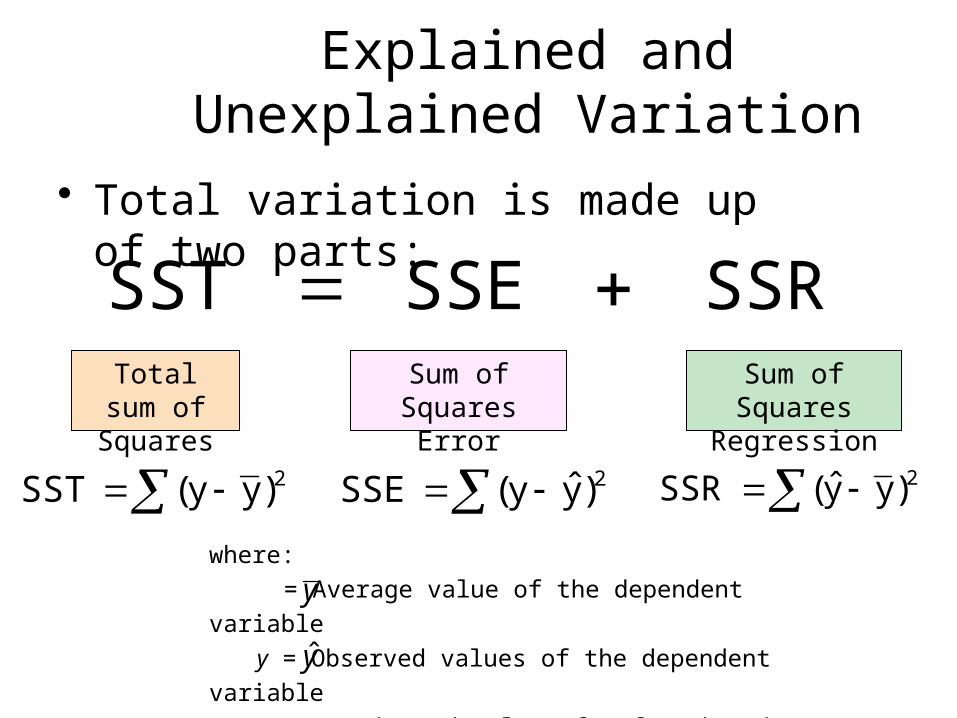
Explained and Unexplained Variation
• Total variation is made up of two parts:
SSR SSE SST Total sum of Squares
Sum of Squares
Regression
Sum of Squares Error
2)yy(SST 2)yy(SSE 2)yy(SSR
where:
= Average value of the dependent variable
y = Observed values of the dependent variable
= Estimated value of y for the given x valuey
y

• SST = total sum of squares
– Measures the variation of the yi values around their mean y
• SSE = error sum of squares
– Variation attributable to factors other than the relationship between x and y
• SSR = regression sum of squares
– Explained variation attributable to the relationship between x and y
Explained and Unexplained Variation
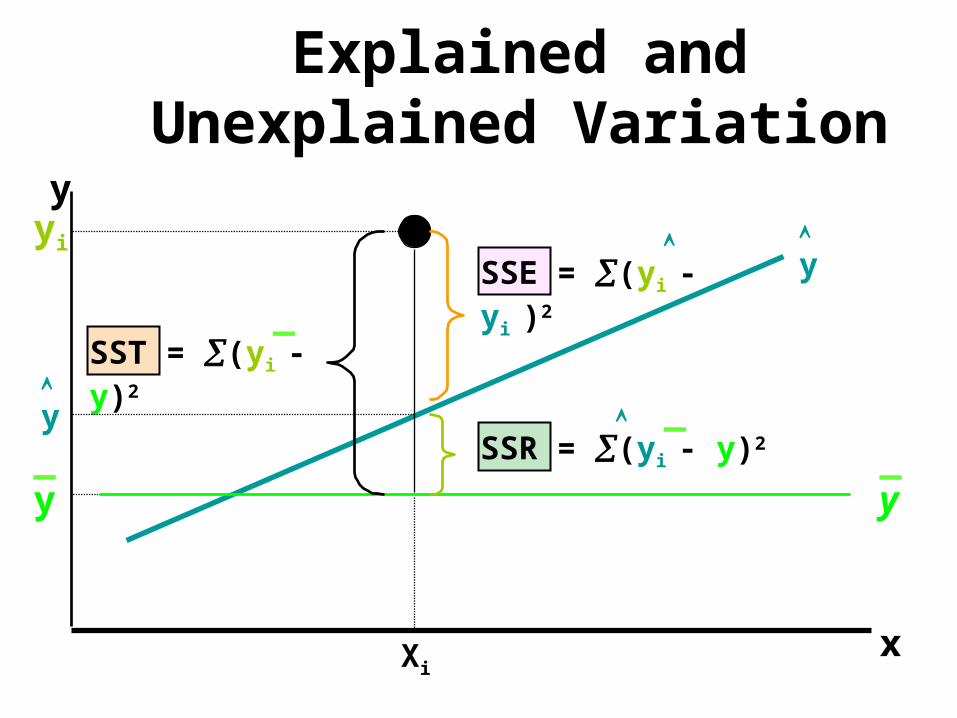
Xi
y
x
yi
SST = (yi - y)2
SSE = (yi - yi )2
SSR = (yi - y)2
_
_
_
Explained and Unexplained Variation
y
y
y_y
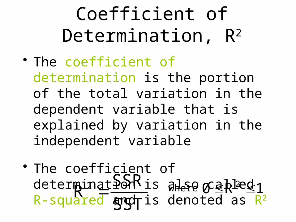
• The coefficient of determination is the portion of the total variation in the dependent variable that is explained by variation in the independent variable
• The coefficient of determination is also called R-squared and is denoted as R2
Coefficient of Determination, R2
SST
SSRR 2 1R0 2 where

Coefficient of determination
Coefficient of Determination, R2
squares of sum total
regressionby explained squares of sum
SST
SSRR 2
Note: In the single independent variable case, the coefficient of determination is
where:R2 = Coefficient of determination
r = Simple correlation coefficient
22 rR
R2 = +1
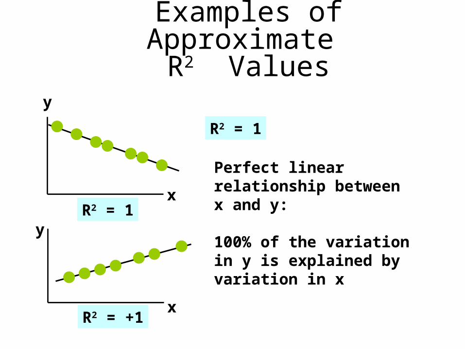
Examples of Approximate R2 Values
y
x
y
x
R2 = 1
R2 = 1
Perfect linear relationship between x and y:
100% of the variation in y is explained by variation in x
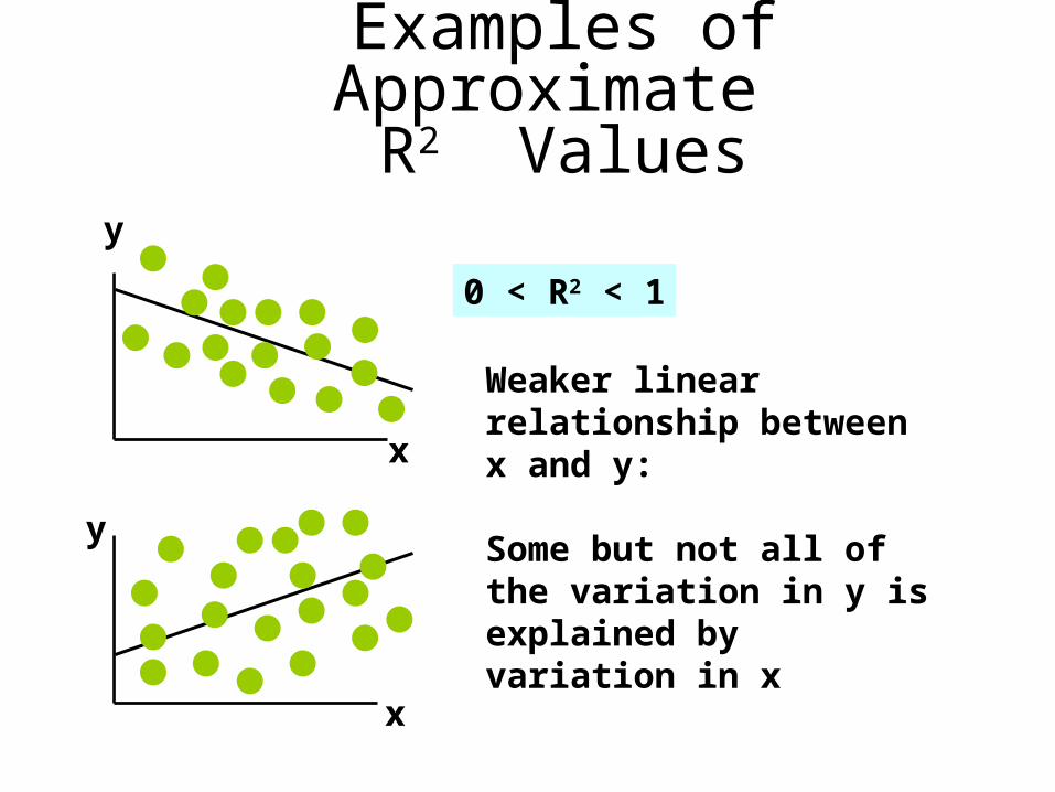
Examples of Approximate R2 Values
y
x
y
x
0 < R2 < 1
Weaker linear relationship between x and y:
Some but not all of the variation in y is explained by variation in x
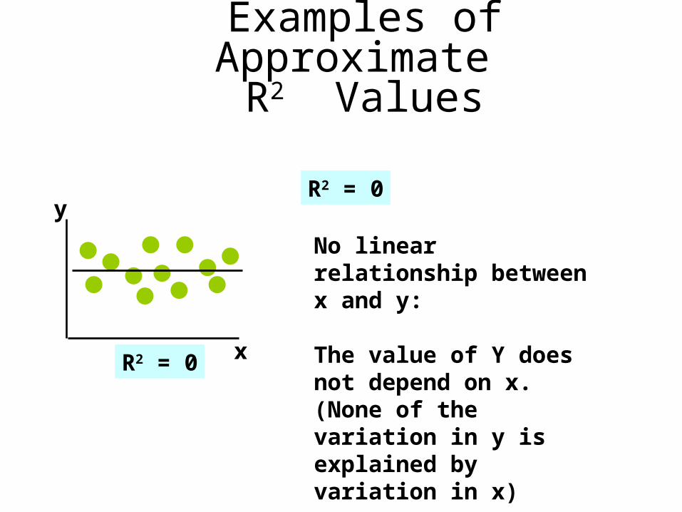
Examples of Approximate R2 Values
R2 = 0
No linear relationship between x and y:
The value of Y does not depend on x. (None of the variation in y is explained by variation in x)
y
xR2 = 0
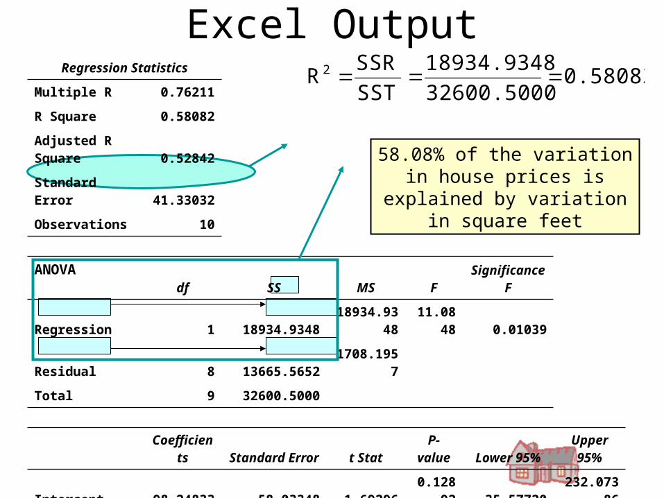
Excel OutputRegression Statistics
Multiple R 0.76211
R Square 0.58082
Adjusted R Square 0.52842
Standard Error 41.33032
Observations 10
ANOVA df SS MS F
Significance F
Regression 1 18934.934818934.934
811.084
8 0.01039
Residual 8 13665.5652 1708.1957
Total 9 32600.5000
Coefficien
ts Standard Error t StatP-
value Lower 95%Upper 95%
Intercept 98.24833 58.03348 1.692960.1289
2 -35.57720232.0738
6
Square Feet 0.10977 0.03297 3.329380.0103
9 0.03374 0.18580
58.08% of the variation in house prices is explained by
variation in square feet
0.5808232600.5000
18934.9348
SST
SSRR2
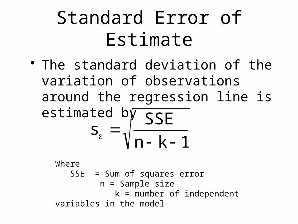
Standard Error of Estimate
• The standard deviation of the variation of observations around the regression line is estimated by
1 kn
SSEs
WhereSSE = Sum of squares error n = Sample size
k = number of independent variables in the model
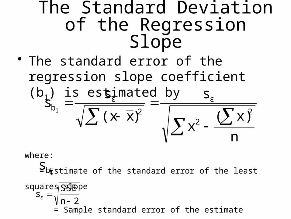
The Standard Deviation of the Regression Slope
• The standard error of the regression slope coefficient (b1) is estimated by
n
x)(x
s
)x(x
ss
22
ε
2
εb1
where:
= Estimate of the standard error of the least squares slope
= Sample standard error of the estimate
1bs
2n
SSEsε
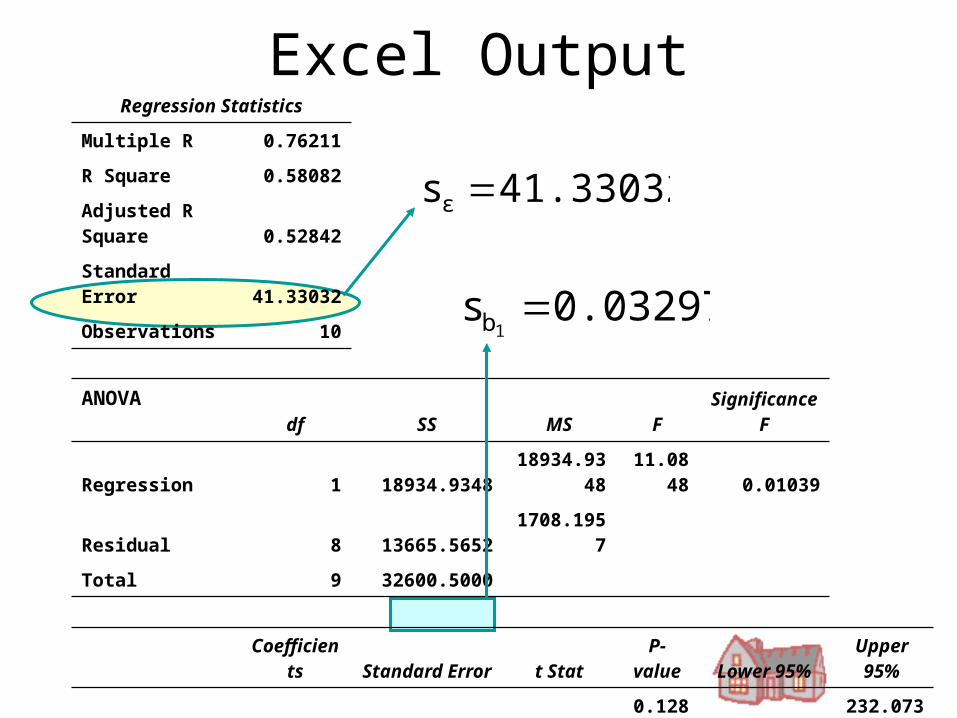
Excel OutputRegression Statistics
Multiple R 0.76211
R Square 0.58082
Adjusted R Square 0.52842
Standard Error 41.33032
Observations 10
ANOVA df SS MS F
Significance F
Regression 1 18934.934818934.934
811.084
8 0.01039
Residual 8 13665.5652 1708.1957
Total 9 32600.5000
Coefficien
ts Standard Error t StatP-
value Lower 95%Upper 95%
Intercept 98.24833 58.03348 1.692960.1289
2 -35.57720232.0738
6
Square Feet 0.10977 0.03297 3.329380.0103
9 0.03374 0.18580
41.33032sε
0.03297s1b
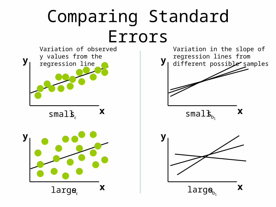
Comparing Standard Errors
y
y y
x
x
x
y
x
1bs small
1bs large
s small
s large
Variation of observed y values from the regression line
Variation in the slope of regression lines from different possible samples
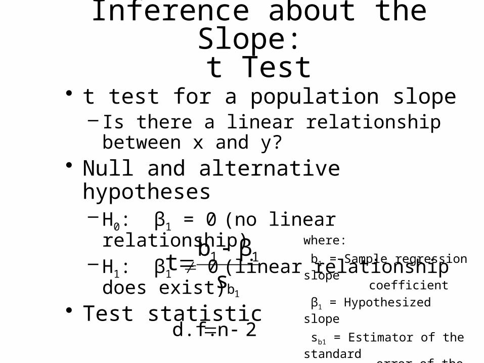
Inference about the Slope: t Test
• t test for a population slope– Is there a linear relationship between x and
y?• Null and alternative hypotheses
– H0: β1 = 0 (no linear relationship)– H1: β1 0 (linear relationship does exist)
• Test statistic
–
–
1b
11
s
βbt
2nd.f.
where:
b1 = Sample regression slope coefficient
β1 = Hypothesized slope
sb1 = Estimator of the standard error of the slope
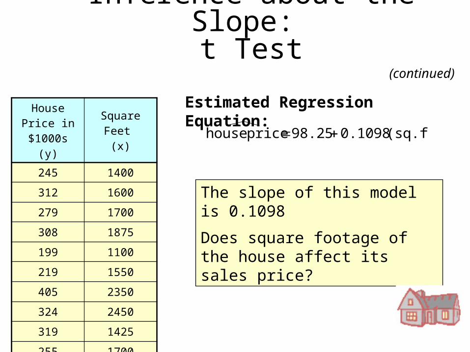
House Price in $1000s
(y)
Square Feet (x)
245 1400
312 1600
279 1700
308 1875
199 1100
219 1550
405 2350
324 2450
319 1425
255 1700
(sq.ft.) 0.1098 98.25 price house
Estimated Regression Equation:
The slope of this model is 0.1098
Does square footage of the house affect its sales price?
Inference about the Slope: t Test
(continued)
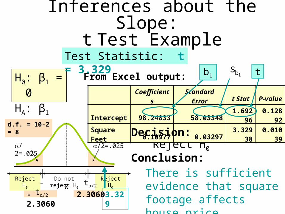
Inferences about the Slope: t Test Example
H0: β1 = 0
HA: β1 0
Test Statistic: t = 3.329
There is sufficient evidence that square footage affects house price
From Excel output:
Reject H0
Coefficient
sStandard
Error t StatP-
value
Intercept 98.24833 58.033481.6929
60.1289
2
Square Feet 0.10977 0.03297
3.32938
0.01039
1bs tb1
Decision:
Conclusion:
Reject H0Reject H0
a/2=.025
-tα/2
Do not reject H0
0 tα/2
a/2=.025
-2.3060 2.3060 3.329
d.f. = 10-2 = 8
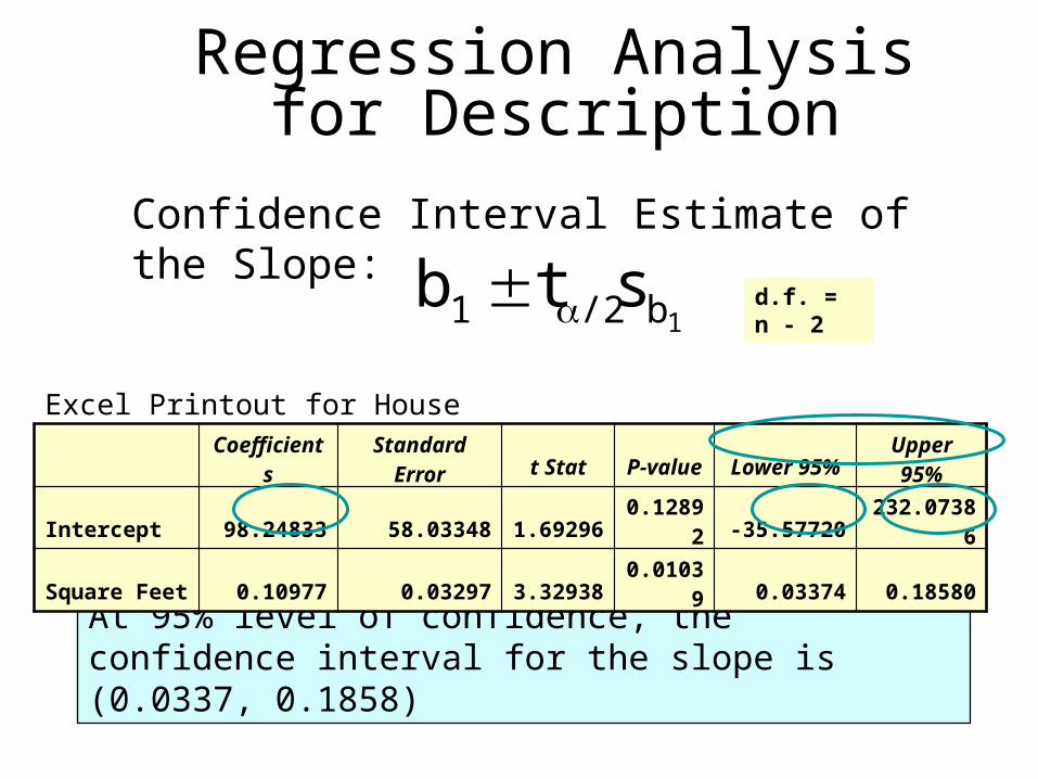
Regression Analysis for Description
Confidence Interval Estimate of the Slope:
Excel Printout for House Prices:
At 95% level of confidence, the confidence interval for the slope is (0.0337, 0.1858)
1b/21 stb
Coefficient
sStandard
Error t Stat P-value Lower 95%Upper 95%
Intercept 98.24833 58.03348 1.69296 0.12892 -35.57720 232.07386
Square Feet 0.10977 0.03297 3.32938 0.01039 0.03374 0.18580
d.f. = n - 2
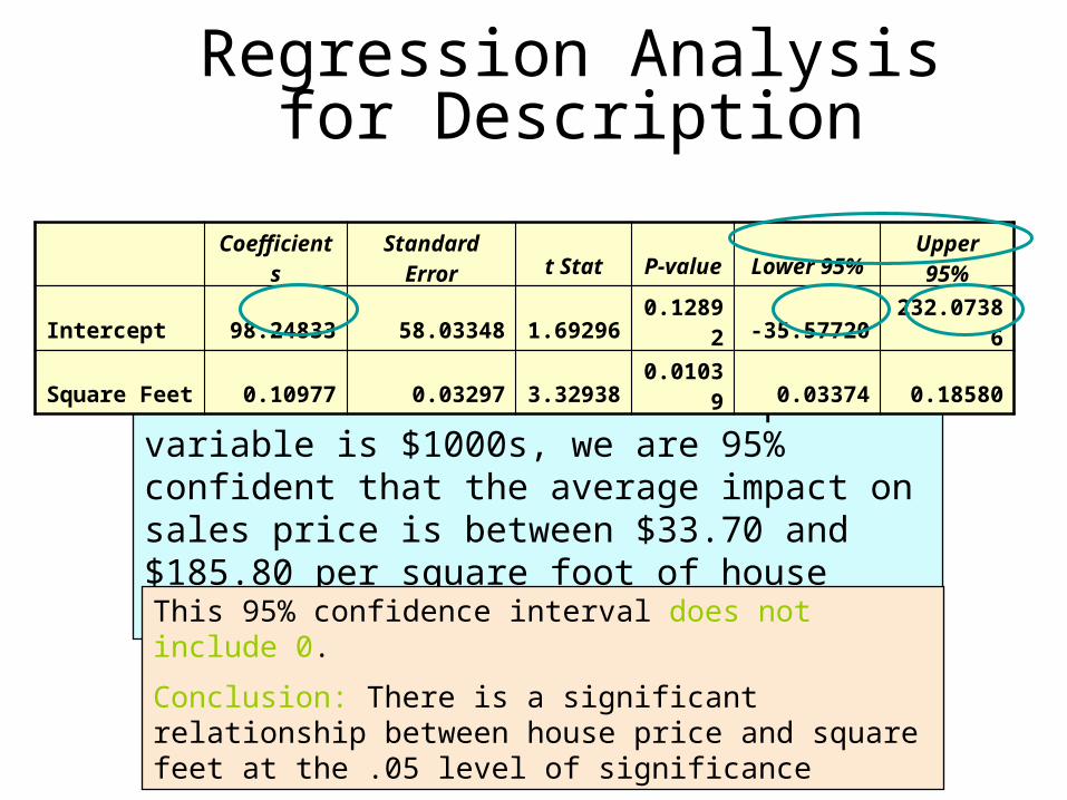
Regression Analysis for Description
Since the units of the house price variable is $1000s, we are 95% confident that the average impact on sales price is between $33.70 and $185.80 per square foot of house size
Coefficient
sStandard
Error t Stat P-value Lower 95%Upper 95%
Intercept 98.24833 58.03348 1.69296 0.12892 -35.57720 232.07386
Square Feet 0.10977 0.03297 3.32938 0.01039 0.03374 0.18580
This 95% confidence interval does not include 0.
Conclusion: There is a significant relationship between house price and square feet at the .05 level of significance
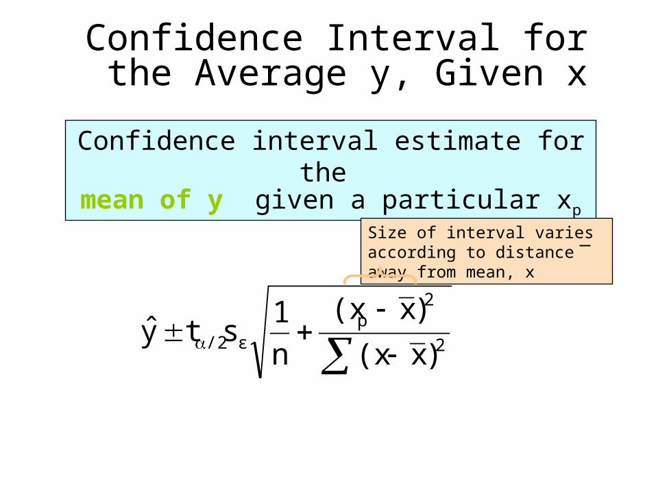
Confidence Interval for the Average y, Given x
Confidence interval estimate for the mean of y given a particular xp
Size of interval varies according to distance away from mean, x
2
2p
ε/2 )x(x
)x(x
n
1sty

Confidence Interval for an Individual y, Given x
Confidence interval estimate for an Individual value of y given a particular xp
2
2p
ε/2 )x(x
)x(x
n
11sty
This extra term adds to the interval width to reflect the added uncertainty for an individual case
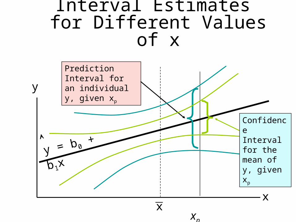
Interval Estimates for Different Values of x
y
x
Prediction Interval for an individual y, given xp
xp
y = b0 + b1x
x
Confidence Interval for the mean of y, given xp
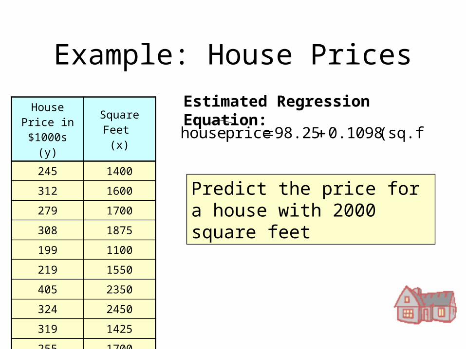
House Price in $1000s
(y)
Square Feet (x)
245 1400
312 1600
279 1700
308 1875
199 1100
219 1550
405 2350
324 2450
319 1425
255 1700
(sq.ft.) 0.1098 98.25 price house
Estimated Regression Equation:
Example: House Prices
Predict the price for a house with 2000 square feet
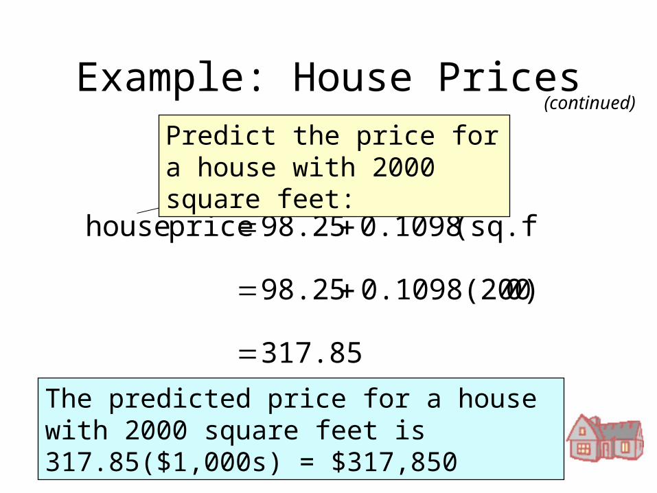
317.85
0)0.1098(200 98.25
(sq.ft.) 0.1098 98.25 price house
Example: House PricesPredict the price for a house with 2000 square feet:
The predicted price for a house with 2000 square feet is 317.85($1,000s) = $317,850
(continued)
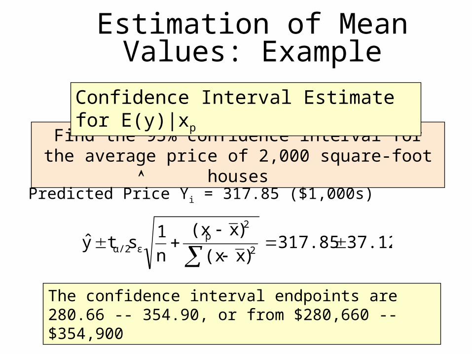
Estimation of Mean Values: Example
Find the 95% confidence interval for the average price of 2,000 square-foot houses
Predicted Price Yi = 317.85 ($1,000s)
Confidence Interval Estimate for E(y)|xp
37.12317.85)x(x
)x(x
n
1sty
2
2p
εα/2
The confidence interval endpoints are 280.66 -- 354.90, or from $280,660 -- $354,900
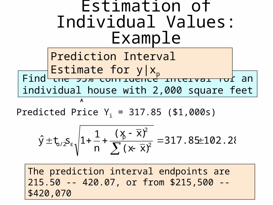
Estimation of Individual Values: Example
Find the 95% confidence interval for an individual house with 2,000 square feet
Predicted Price Yi = 317.85 ($1,000s)
Prediction Interval Estimate for y|xp
102.28317.85)x(x
)x(x
n
11sty
2
2p
εα/2
The prediction interval endpoints are 215.50 -- 420.07, or from $215,500 -- $420,070