1

LINEAR STABILITY THEORY

Serkan Özgen, Prof. Dr.

Middle East Technical University, Dept. Aerospace Eng., Turkey

1. Introduction

Hydrodynamic stability is known as one of the most important and yet least understood fields

of fluid mechanics since more than a century. Its main concern is to investigate the breakdown

of laminar flows, their subsequent development and eventual transition to turbulent flow. A

few of the practical applications of this subject are: laminar flow control of wings of large

transport aircraft in order to save in fuel consumption, prediction of transition location on

airfoils for accurate heat transfer prediction and blade cooling in turbomachinery, and jet flows

for more efficient combustion in gas turbine and internal combustion engines, etc.

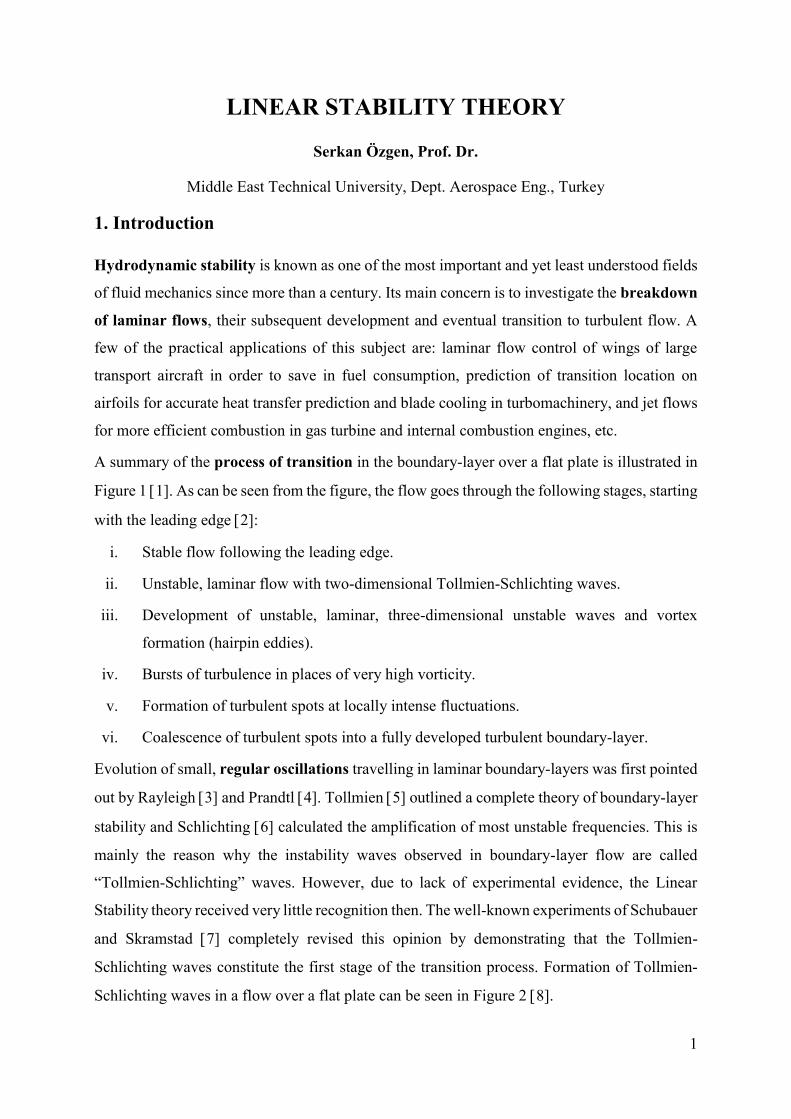
A summary of the process of transition in the boundary-layer over a flat plate is illustrated in

Figure 1 1]. As can be seen from the figure, the flow goes through the following stages, starting

with the leading edge 2]:

i. Stable flow following the leading edge.

ii. Unstable, laminar flow with two-dimensional Tollmien-Schlichting waves.

iii. Development of unstable, laminar, three-dimensional unstable waves and vortex

formation (hairpin eddies).

iv. Bursts of turbulence in places of very high vorticity.

v. Formation of turbulent spots at locally intense fluctuations.

vi. Coalescence of turbulent spots into a fully developed turbulent boundary-layer.

Evolution of small, regular oscillations travelling in laminar boundary-layers was first pointed

out by Rayleigh 3] and Prandtl 4]. Tollmien 5] outlined a complete theory of boundary-layer

stability and Schlichting 6] calculated the amplification of most unstable frequencies. This is

mainly the reason why the instability waves observed in boundary-layer flow are called

“Tollmien-Schlichting” waves. However, due to lack of experimental evidence, the Linear

Stability theory received very little recognition then. The well-known experiments of Schubauer

and Skramstad 7] completely revised this opinion by demonstrating that the Tollmien-

Schlichting waves constitute the first stage of the transition process. Formation of Tollmien-

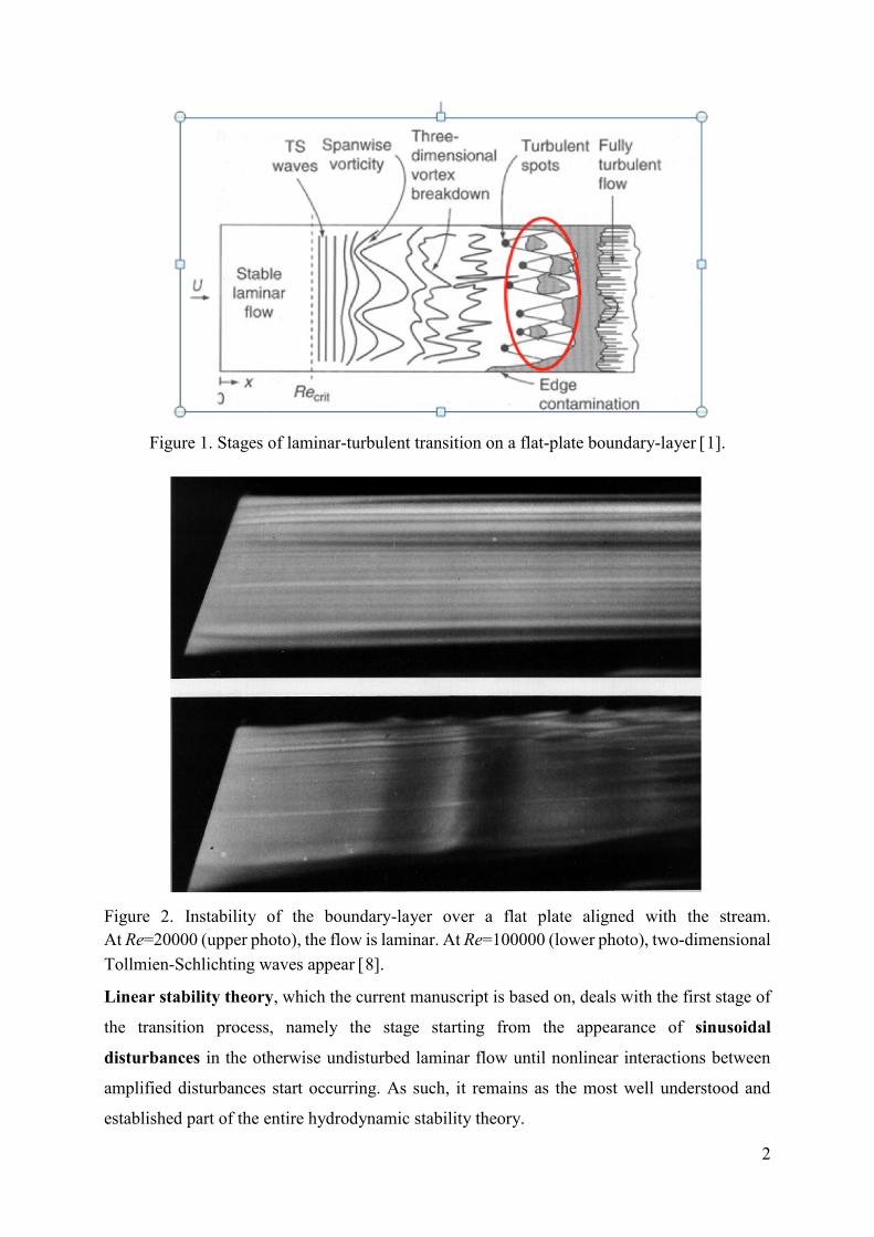
Schlichting waves in a flow over a flat plate can be seen in Figure 2 8].

2

Figure 1. Stages of laminar-turbulent transition on a flat-plate boundary-layer 1].

Figure 2. Instability of the boundary-layer over a flat plate aligned with the stream.

At Re=20000 (upper photo), the flow is laminar. At Re=100000 (lower photo), two-dimensional

Tollmien-Schlichting waves appear 8].

Linear stability theory, which the current manuscript is based on, deals with the first stage of

the transition process, namely the stage starting from the appearance of sinusoidal

disturbances in the otherwise undisturbed laminar flow until nonlinear interactions between

amplified disturbances start occurring. As such, it remains as the most well understood and

established part of the entire hydrodynamic stability theory.

3

In this manuscript, the Linear Stability Theory is outlined resulting in the stability equations.

The theory is described for a three-dimensional, steady, incompressible mean flow but it is also

applicable to other regimes, see Reference 9]. Well-known and established methods are

introduced to clearly illustrate the basics of the theory and to make it easier for the reader to

follow the literature. Method of small disturbances, method of normal modes, temporal and

spatial formulations, Gaster’s Transformation, Orr-Sommerfeld equation and Squire’s Theorem

are explained. Solution of the eigenvalue problem is also outlined together with the application

of the theory to two- and three-dimensional boundary-layer flows.

2. Formulation of the Linear Stability Theory

2.1. Basic Flow

In order to perform the stability analysis of a flow, velocity �⃗⃗� ∗(𝑥 ∗, 𝑡∗), pressure 𝑃∗(𝑥 ∗, 𝑡∗) and

temperature 𝑇∗(𝑥 ∗, 𝑡∗) fields must be known. These fields define the basic flow. The basic flow

may be steady or unsteady, two-dimensional or three-dimensional, incompressible or

compressible and even Newtonian or non-Newtonian, but in any case must satisfy the

corresponding equations of motion.

2.2. Method of Small Disturbances

We shall make use of the method of small disturbances, which leads to a linear problem.

Equations of motion for a three-dimensional, incompressible flow in Cartesian coordinates are

(asterisks denote dimensional quantities, while 𝑔∗ denotes gravitational acceleration):

𝜕𝑢∗

𝜕𝑡∗ + 𝑢∗ 𝜕𝑢∗

𝜕𝑥∗ + 𝑣∗ 𝜕𝑢∗

𝜕𝑦∗ + 𝑤∗ 𝜕𝑢∗

𝜕𝑧∗ = −1

𝜌∗

𝜕𝑝∗

𝜕𝑥∗ +1

𝜌∗ (𝜕𝜎𝑥𝑥

∗

𝜕𝑥∗ +𝜕𝜏𝑥𝑦

∗

𝜕𝑦∗ +𝜕𝜏𝑥𝑧

∗

𝜕𝑧∗ ), (1)

𝜕𝑣∗

𝜕𝑡∗ + 𝑢∗ 𝜕𝑣∗

𝜕𝑥∗ + 𝑣∗ 𝜕𝑣∗

𝜕𝑦∗ + 𝑤∗ 𝜕𝑣∗

𝜕𝑧∗ = −1

𝜌∗

𝜕𝑝∗

𝜕𝑦∗ +1

𝜌∗ (𝜕𝜏𝑦𝑥

∗

𝜕𝑥∗ +𝜕𝜎𝑦𝑦

∗

𝜕𝑦∗ +𝜕𝜏𝑦𝑧

∗

𝜕𝑧∗ ) − 𝑔∗, (2)

𝜕𝑤∗

𝜕𝑡∗+ 𝑢∗ 𝜕𝑤∗

𝜕𝑥∗+ 𝑣∗ 𝜕𝑤∗

𝜕𝑦∗+ 𝑤∗ 𝜕𝑤∗

𝜕𝑧∗= −

1

𝜌∗

𝜕𝑝∗

𝜕𝑧∗+

1

𝜌∗(𝜕𝜏𝑧𝑥

∗

𝜕𝑥∗+

𝜕𝜏𝑧𝑦∗

𝜕𝑦∗+

𝜕𝜎𝑧𝑧∗

𝜕𝑧∗), (3)

𝜕𝑢∗

𝜕𝑥∗ +𝜕𝑣∗

𝜕𝑦∗ +𝜕𝑤∗

𝜕𝑧∗ = 0. (4)

In the above equations, 𝜌∗ denotes the density of the fluid. The stress terms are defined as:

𝜎𝑥𝑥∗ = 2𝜇∗ 𝜕𝑢∗

𝜕𝑥∗ , 𝜎𝑦𝑦∗ = 2𝜇∗ 𝜕𝑣∗

𝜕𝑦∗ , 𝜎𝑧𝑧∗ = 2𝜇∗ 𝜕𝑤∗

𝜕𝑧∗ , (5)

𝜏𝑥𝑦∗ = 𝜏𝑦𝑥

∗ = 𝜇∗ (𝜕𝑢∗

𝜕𝑦∗+

𝜕𝑣∗

𝜕𝑥∗) , (6)

𝜏𝑥𝑧∗ = 𝜏𝑧𝑥

∗ = 𝜇∗ (𝜕𝑢∗

𝜕𝑧∗ +𝜕𝑤∗

𝜕𝑥∗) , (7)

𝜏𝑦𝑧∗ = 𝜏𝑧𝑦

∗ = 𝜇∗ (𝜕𝑣∗

𝜕𝑧∗+

𝜕𝑤∗

𝜕𝑦∗) . (8)

4

In the above equations, 𝜇∗ is the viscosity of the fluid.

The flow is decomposed into steady mean and unsteady perturbations as follows:

𝑢∗(𝑥∗, 𝑦∗, 𝑧∗, 𝑡∗) = 𝑈∗(𝑥∗, 𝑦∗, 𝑧∗) + �̂�∗(𝑥∗, 𝑦∗, 𝑧∗, 𝑡∗), (9)

𝑣∗(𝑥∗, 𝑦∗, 𝑧∗, 𝑡∗) = 𝑉∗(𝑥∗, 𝑦∗, 𝑧∗) + 𝑣∗(𝑥∗, 𝑦∗, 𝑧∗, 𝑡∗), (10)

𝑤∗(𝑥∗, 𝑦∗, 𝑧∗, 𝑡∗) = 𝑊∗(𝑥∗, 𝑦∗, 𝑧∗) + �̂�∗(𝑥∗, 𝑦∗, 𝑧∗, 𝑡∗), (11)

𝑝∗(𝑥∗, 𝑦∗, 𝑧∗, 𝑡∗) = 𝑃∗(𝑥∗, 𝑦∗, 𝑧∗) + �̂�∗(𝑥∗, 𝑦∗, 𝑧∗, 𝑡∗). (12)

The problem is further simplified when the parallel flow assumption is employed.

Accordingly, 𝑈∗ = 𝑈∗(𝑦∗),𝑊∗ = 𝑊∗(𝑦∗) only, and 𝑉∗ = 0. In a channel flow, such a flow is

reproduced with great accuracy at a large distance from the inlet. Boundary-layer flow can also

be regarded as a good approximation because 𝑈∗ ≫ 𝑉∗ and 𝜕 𝜕𝑦∗ ≫⁄ 𝜕 𝜕𝑥∗⁄ . For pressure, it

is necessary to retain dependence both on 𝑥∗ and 𝑦∗, because pressure gradient 𝜕𝑝∗ 𝜕𝑥∗⁄ drives

the flow in most cases. Therefore, equations (7-9) can be rewritten as:

𝑢∗(𝑥∗, 𝑦∗, 𝑧∗, 𝑡∗) = 𝑈∗(𝑦∗) + �̂�∗(𝑥∗, 𝑦∗, 𝑧∗, 𝑡∗), (13)

𝑣∗(𝑥∗, 𝑦∗, 𝑧∗, 𝑡∗) = 𝑣∗(𝑥∗, 𝑦∗, 𝑧∗, 𝑡∗), (14)

𝑤∗(𝑥∗, 𝑦∗, 𝑧∗, 𝑡∗) = 𝑊∗(𝑦∗) + �̂�∗(𝑥∗, 𝑦∗, 𝑧∗, 𝑡∗), (15)

𝑝∗(𝑥∗, 𝑦∗, 𝑧∗, 𝑡∗) = 𝑃∗(𝑥∗, 𝑦∗, 𝑧∗) + �̂�∗(𝑥∗, 𝑦∗, 𝑧∗, 𝑡∗). (16)

In the next step, the flow defined in equations (13-16) is substituted into equations (1-4).

Unsteady perturbations are small with respect to their counterparts, i.e. �̂�∗, 𝑣∗ ≪ 𝑈∗, therefore

quadratic terms like �̂�∗ 𝜕�̂�∗ 𝜕𝑥∗⁄ are dropped out and the following set of equations result:

𝜕𝑢∗

𝜕𝑡∗ + 𝑈∗ 𝜕𝑢∗

𝜕𝑥∗ + 𝑣∗ 𝑑𝑈∗

𝑑𝑦∗ + 𝑊∗ 𝜕𝑢∗

𝜕𝑧∗ = −1

𝜌∗ (𝜕𝑃∗

𝜕𝑥∗ +𝜕𝑝∗

𝜕𝑥∗) + 𝜈∗ (𝑑2𝑈∗

𝑑𝑦∗2 +𝜕2𝑢∗

𝜕𝑥∗2 +𝜕2𝑢∗

𝜕𝑦∗2 +𝜕2�̂�∗

𝜕𝑧∗2), (17)

𝜕�̂�∗

𝜕𝑡∗+ 𝑈∗ 𝜕�̂�∗

𝜕𝑥∗+ 𝑊∗ 𝜕�̂�∗

𝜕𝑧∗= −

1

𝜌∗(𝜕𝑃∗

𝜕𝑦∗+

𝜕𝑝∗

𝜕𝑦∗) + 𝜈∗ (

𝜕2�̂�∗

𝜕𝑥∗2+

𝜕2�̂�∗

𝜕𝑦∗2+

𝜕2�̂�∗

𝜕𝑧∗2) − 𝑔∗, (18)

𝜕�̂�∗

𝜕𝑡∗+ 𝑈∗ 𝜕�̂�∗

𝜕𝑥∗+ 𝑣∗ 𝑑𝑊∗

𝑑𝑦∗+ 𝑊∗ 𝜕�̂�∗

𝜕𝑧∗= −

1

𝜌∗(𝜕𝑃∗

𝜕𝑧∗+

𝜕𝑝∗

𝜕𝑧∗) + 𝜈∗ (

𝑑2𝑊∗

𝑑𝑦∗2+

𝜕2�̂�∗

𝜕𝑥∗2+

𝜕2�̂�∗

𝜕𝑦∗2+

𝜕2�̂�∗

𝜕𝑧∗2) (19)

𝜕𝑢∗

𝜕𝑥∗+

𝜕�̂�∗

𝜕𝑦∗+

𝜕�̂�∗

𝜕𝑧∗= 0. (20)

In the above equations, 𝜈∗ = 𝜇∗/𝜌∗ is the kinematic viscosity of the fluid. It is worth mentioning

that the perturbation velocities satisfy the continuity equation.

At this point, non-dimensionalization of velocities with an appropriate velocity scale 𝑈𝑟𝑒𝑓∗ , and

lengths with an appropriate length scale 𝑑𝑟𝑒𝑓∗ is performed. Accordingly, time is normalized by

𝑑𝑟𝑒𝑓∗ /𝑈𝑟𝑒𝑓

∗ and pressure by 𝜌∗𝑈𝑟𝑒𝑓∗2 .

5

After the terms involving only the basic flow quantities are dropped, the following set of

equations is obtained:

𝜕𝑢

𝜕𝑡+ 𝑈

𝜕𝑢

𝜕𝑥+ 𝑊

𝜕𝑢

𝜕𝑧+ 𝑣

𝑑𝑈

𝑑𝑦= −

𝜕𝑝

𝜕𝑥+

1

𝑅𝑒(𝜕2�̂�

𝜕𝑥2 +𝜕2�̂�

𝜕𝑦2 +𝜕2𝑢

𝜕𝑧2), (21)

𝜕�̂�

𝜕𝑡+ 𝑈

𝜕�̂�

𝜕𝑥+ 𝑊

𝜕�̂�

𝜕𝑧= −

𝜕𝑝

𝜕𝑦+

1

𝑅𝑒(𝜕2�̂�

𝜕𝑥2+

𝜕2�̂�

𝜕𝑦2+

𝜕2�̂�

𝜕𝑧2), (22)

𝜕�̂�

𝜕𝑡+ 𝑈

𝜕�̂�

𝜕𝑥+ 𝑊

𝜕�̂�

𝜕𝑧+ 𝑣

𝑑𝑊

𝑑𝑦= −

𝜕𝑝

𝜕𝑧+

1

𝑅𝑒(𝜕2�̂�

𝜕𝑥2 +𝜕2�̂�

𝜕𝑦2 +𝜕2�̂�

𝜕𝑧2), (23)

𝜕𝑢

𝜕𝑥+

𝜕�̂�

𝜕𝑦+

𝜕�̂�

𝜕𝑧= 0. (24)

In the above equations, Reynolds number is defined as 𝑅𝑒 = 𝑈𝑟𝑒𝑓∗ 𝑑𝑟𝑒𝑓

∗ /𝜈∗. In equation (18):

−1

𝜌∗

𝜕𝑃∗

𝜕𝑦∗ − 𝑔∗ = 0 or 𝜕𝑃

𝜕𝑦+ 𝐹𝑟−2 = 0, (25)

where 𝐹𝑟 = 𝑈𝑟𝑒𝑓∗ /(𝑔∗𝑑𝑟𝑒𝑓

∗ )1/2 is the Froude number.

2.3. Method of Normal Modes

The basic laminar flow in x-direction is assumed to be influenced by a disturbance composed

of a number of discrete partial fluctuations each consisting of a wave propagating in x-direction.

Perturbation velocities corresponding to each component can be defined as:

[�̂�, 𝑣, �̂�, �̂�] = [�̅�, �̅�, �̅�, �̅�](𝑦)𝑒𝑖(𝛼𝑥+𝛽𝑧−𝜔𝑡), 𝑗 = 1, 2, 3, … (26)

In the above equation, �̅�(𝑦), �̅�(𝑦), �̅�(𝑦) and �̅�(𝑦) are the disturbance amplitude functions

for the perturbations �̂�, 𝑣, �̂� and �̂�. The disturbance wavenumber components are 𝛼 and 𝛽.

The frequency of the disturbance is denoted by 𝜔. In the general formulation, wavenumber

components 𝛼 and 𝛽, and the frequency 𝜔 are complex.

Normal mode decomposition is a Fourier analysis of the disturbance modes based on the fact

that all the coefficients in equations (21-24) are functions of 𝑦 only, admitting Fourier modes

in 𝑥, 𝑧 and 𝑡.

When the definitions in equation (26) are substituted into equations (21-24), the following

system of equations result (primes (′) denoting differentiation with respect to 𝑦):

𝑖(𝛼𝑈 + 𝛽𝑊 − 𝜔)�̅� + 𝑈′�̅� = −𝑖𝛼�̅� +1

𝑅𝑒[�̅�′′ − (𝛼2 + 𝛽2)�̅�], (27)

𝑖(𝛼𝑈 + 𝛽𝑊 − 𝜔)�̅� = −�̅�′ +1

𝑅𝑒[�̅�′′ − (𝛼2 + 𝛽2)�̅�], (28)

𝑖(𝛼𝑈 + 𝛽𝑊 − 𝜔)�̅� + 𝑊′�̅� = −𝑖𝛽�̅� +1

𝑅𝑒[�̅�′′ − (𝛼2 + 𝛽2)�̅�], (29)

𝑖(𝛼�̅� + 𝛽�̅�) + �̅�′ = 0. (30)

6

Equations (27-30) are the perturbation equations for a three-dimensional basic flow in a three-

dimensional disturbance environment. They constitute a sixth order system for the variables

�̅�, �̅�, �̅�, �̅�, �̅�′ and �̅�′. The boundary conditions are:

�̅�(0) = �̅�(0) = �̅�(0) = 0, (no slip) (31)

�̅�(𝑦) → 0, �̅�(𝑦) → 0, �̅�(𝑦) → 0 as 𝑦 → ∞. (freestream) (32)

2.4. Temporal and Spatial Amplification Formulations

2.4.1. Spatial Amplification Formulation

In this formulation, the local mode is given as in equation (26). The wave number components

are complex, i.e. 𝛼 = 𝛼𝑟 + 𝑖𝛼𝑖 and 𝛽 = 𝛽𝑟 + 𝑖𝛽𝑖, while the frequency 𝜔 is real.

A real wavenumber vector can be defined with magnitude:

𝑘 = (𝛼𝑟2 + 𝛽𝑟

2)1/2, (33)

and a wave angle:

Ψ = tan−1(𝛽𝑟 𝛼𝑟)⁄ . (34)

The phase speed of the wave is defined as 𝑐 = 𝜔/𝑘.

Accordingly, in spatial amplification formulation, equation (26) can be written as follows:

[�̂�, 𝑣, �̂�, �̂�] = [�̅�, �̅�, �̅�, �̅�](𝑦)𝑒−𝛼𝑖𝑥𝑒𝑖(𝛼𝑟𝑥+𝛽𝑧−𝜔𝑡). (35)

The spatial amplification rate is −𝛼𝑖 for which:

𝛼𝑖 < 0; unstable wave,

𝛼𝑖 = 0; neutrally stable wave,

𝛼𝑖 > 0; stable wave.

The dispersion relation is given as 𝛼 = 𝑓(𝜔, 𝛽, 𝑅𝑒).

2.4.2. Temporal Amplification Formulation

In this formulation, the local mode is still given as in equation (26) but this time the

wavenumbers 𝛼 and 𝛽 are real and the frequency is complex, 𝜔 = 𝜔𝑟 + 𝑖𝜔𝑖. Therefore, phase

velocity is also complex, 𝑐 = 𝜔 𝛼 =⁄ 𝑐𝑟 + 𝑖𝑐𝑖. The phase speed of the wave is 𝑐𝑟, and 𝑐𝑖 is the

temporal amplification factor.

Real wavenumber vector magnitude is given as:

𝑘 = (𝛼2 + 𝛽2)1/2, (36)

while the wave angle is:

Ψ = tan−1(𝛽 𝛼⁄ ). (37)

7

Accordingly, equation (26) can be written as follows:

[�̂�, 𝑣, �̂�, �̂�] = [�̅�, �̅�, �̅�, �̅�](𝑦)𝑒𝛼𝑐𝑖𝑡𝑒𝑖(𝛼𝑥+𝛽𝑧−𝛼𝑐𝑟𝑡). (38)

The temporal amplification rate is 𝜔𝑖 = 𝛼𝑐𝑖 for which:

𝑐𝑖 > 0; unstable wave,

𝑐𝑖 = 0; neutrally stable wave,

𝑐𝑖 < 0; stable wave.

The dispersion relation is given as 𝑐 = 𝑓(𝛼, 𝛽, 𝑅𝑒).

Since the eigenvalue 𝑐 appears linearly in the temporal form of the differential equations, most

of the early studies reported in the literature are concentrated on this formulation. However,

spatial modes seem to describe the observed instability of parallel flows more faithfully then

temporal modes.

2.4.3. Gaster’s Transformation

It has been shown that simple relations exist between the parameters arising in temporal and

spatial amplification formulations 10]. These relations do not constitute a transformation of a

time-dependent solution into a spatially dependent one but merely provide a link between the

values of the parameters existing in the two problems. Accordingly, the real parts of the

wavenumbers and phase velocities are equal in both cases; 𝛼(𝑇) = 𝛼𝑟(𝑆), 𝛽(𝑇) = 𝛽𝑟(𝑇) and

𝑐𝑟(𝑇) = 𝑐(𝑆). It follows that:

𝜔𝑖(𝑇)

𝛼𝑖(𝑆)= −

𝜕𝜔𝑟

𝜕𝛼. (41)

The quantity on the right side of the equation is the group velocity and the relation given in

this equation is the Gaster’s transformation. It merely means that the spatial growth of a mode

is related to the temporal growth by the group velocity but not the phase velocity.

2.5. Reduction to Fourth Order System

A new set of equations can be obtained by producing linear combinations of equations (27) and

(29). Equations (27) and (29) are multiplied by 𝛼 and 𝛽, respectively, and added; equation (27)

multiplied by 𝛽 is subtracted from equation (29) multiplied by 𝛼:

𝑖(𝛼𝑈 + 𝛽𝑊 − 𝜔)(𝛼�̅� + 𝛽�̅�) + (𝛼𝑈′ + 𝛽𝑊′)�̅� = −𝑖(𝛼2 + 𝛽2)�̅� +1

𝑅𝑒[𝐷2 − (𝛼2 + 𝛽2)](𝛼�̅� + 𝛽�̅�), (42)

𝑖(𝛼𝑈 + 𝛽𝑊 − 𝜔)�̅� = −�̅�′ +1

𝑅𝑒[�̅�′′ − (𝛼2 + 𝛽2)�̅�], (43)

𝑖(𝛼𝑈 + 𝛽𝑊 − 𝜔)(𝛼�̅� − 𝛽�̅�) + (𝛼𝑊′ − 𝛽𝑈′)�̅� = +1

𝑅𝑒[𝐷2 − (𝛼2 + 𝛽2)](𝛼�̅� − 𝛽�̅�), (44)

𝑖(𝛼�̅� + 𝛽�̅�) + �̅�′ = 0. (45)

8

In this formulation, the dependent variables are 𝛼�̅� + 𝛽�̅�, �̅�, �̅� and 𝛼�̅�′ + 𝛽�̅�′. Noticing that

the variable 𝛼�̅� − 𝛽�̅� appears only in equation (44), the remaining equations constitute a fourth

order system for the solution of the eigenvalues 𝛼, 𝛽, 𝜔 and 𝑅𝑒. In physical terms, equation

(42) is the momentum equation in the direction of the wave motion, while equation (44) is the

momentum equation in the direction perpendicular to wave motion.

2.6. Orr-Sommerfeld Equation

In equation (42), when the (𝛼�̅� + 𝛽�̅�) term is eliminated by using equation (45) and the

pressure term is eliminated by using equation (43), a single fourth order equation results:

�̅�′′′′ − 2(𝛼2 + 𝛽2)�̅�′′ + (𝛼2 + 𝛽2)2�̅� = 𝑖𝑅𝑒{(𝛼𝑈 + 𝛽𝑊 − 𝜔)[�̅�′′ − (𝛼2 + 𝛽2)�̅�] − (𝛼𝑈′′ + 𝛽𝑊′′)�̅�}. (46)

This is the well-known Orr-Sommerfeld equation, which has been the basis for many studies

related to incompressible flow study. The accompanying boundary conditions are:

�̅�(0) = �̅�′(0) = 0, (no slip) (47)

�̅�(𝑦) → 0, �̅�′(𝑦) → 0 as 𝑦 → ∞. (freestream) (48)

The same equation can be derived in terms of a disturbance streamfunction for a two-

dimensional basic flow and a two-dimensional disturbance environment, as detailed in

References 2, 11] and many others:

𝜙′′′′ − 2𝛼2𝜙′′ + 𝛼4𝜙 = 𝑖𝑅𝑒{(𝛼𝑈 − 𝜔)[𝜙′′ − 𝛼2𝜙] − 𝛼𝑈′′𝜙}, (49)

or �̅�′′′′ − 2𝛼2�̅�′′ + 𝛼4�̅� = 𝑖𝑅𝑒{(𝛼𝑈 − 𝜔)[�̅�′′ − 𝛼2�̅�] − 𝛼𝑈′′�̅�}. (50)

2.7. Squire’s Transformation and Squire’s Theorem

For a two-dimensional basic flow (𝑊 = 0), the following transformation is considered:

�̃�2 = 𝛼2 + 𝛽2, �̃��̃� = 𝛼�̅� + 𝛽�̅�, �̃�

�̃�=

�̅�

𝛼 , �̃� = 𝑐,

�̃� = 𝑣, �̃�𝑅�̃� = 𝛼𝑅𝑒, �̃�𝑅�̃� = 𝜔𝑅𝑒. (51)

With this, equations (27-30) become:

𝑖(�̃�𝑈 − �̃�)�̃� + 𝑈′�̃� = −𝑖�̃�𝑝 +1

𝑅�̃�(�̃�′′ − �̃�2�̃�), (52)

𝑖(�̃�𝑈 − �̃�)�̃� = −𝑝′ +1

𝑅�̃�(�̃�′′ − �̃�2�̃�), (53)

𝑖�̃��̃� + �̃�′ = 0. (54)

The three-dimensional problem defined by equations (27-30) has been reduced to an equivalent

two-dimensional problem. This transformation relates the eigenvalues of an oblique temporal

wave with frequency 𝜔, at Reynolds number 𝑅𝑒, to a two-dimensional wave with frequency �̃�

in a two-dimensional boundary-layer at Reynolds number 𝑅�̃�.

9

Since �̃�2 = 𝛼2 + 𝛽2 ≥ 𝛼2, it follows that 𝑅�̃� ≤ 𝑅𝑒. Therefore, according to Squire’s

Theorem, two-dimensional disturbances yield the lowest limit of stability. In other words, in

order to obtain the minimum critical Reynolds number, it is sufficient to consider two-

dimensional disturbances only.

3. Solution Method 12]

In the solution method that is outlined below, temporal amplification formulation is used due

to its simpler and more straightforward solution. This does not reduce its validity or accuracy

and the method that is outlined can be extended to handle compressible flows, flows with

variable fluid properties, etc. 13, 14, 15].

3.1. System of First Order Equations

Defining the following variables:

𝑌1 = 𝛼�̅� + 𝛽�̅�, (55)

𝑌2 = 𝛼�̅�′ + 𝛽�̅�′, (56)

𝑌3 = �̅�, (57)

𝑌4 = �̅�, (58)

𝑌5 = 𝛼�̅� − 𝛽�̅�, (59)

𝑌6 = 𝛼�̅�′ − 𝛽�̅�′, (60)

equations (42-45) can be written as:

𝑌1′ = 𝑌2, (61)

𝑌2′ = [𝛼2 + 𝛽2 + 𝑖𝑅𝑒(𝛼𝑈 + 𝛽𝑊 − 𝜔)]𝑌1 + 𝑅𝑒(𝛼𝑈′ + 𝛽𝑊′)𝑌3 + 𝑖𝑅𝑒(𝛼2 + 𝛽2)𝑌4, (62)

𝑌3′ = −𝑖𝑌1, (63)

𝑌4′ = −

𝑖

𝑅𝑒𝑌2 − [

𝛼2+𝛽2

𝑅𝑒+ 𝑖(𝛼𝑈 + 𝛽𝑊 − 𝜔)] 𝑌3, (64)

𝑌5′ = 𝑌6, (65)

𝑌6′ = 𝑅𝑒(𝛼𝑊′ − 𝛽𝑈′)𝑌3 + [𝛼2 + 𝛽2 + 𝑖𝑅𝑒(𝛼𝑈 + 𝛽𝑊 − 𝜔)]𝑌5. (66)

Boundary conditions:

𝑌1(0) = 𝑌3(0) = 𝑌5(0) = 0, (no slip) (67)

𝑌1(𝑦) → 0, 𝑌3(𝑦) → 0, 𝑌5(𝑦) → 0 as 𝑦 → ∞. (freestream) (68)

Eigenvalues 𝛼, 𝛽, 𝜔 and 𝑅𝑒 can be computed by solving equations (61-64) only because

variables 𝑌5 and 𝑌6 appear only in equations (65) and (66). In other words, equations (65) and

(66) are decoupled from equations (61-64).

10

3.2. Characteristic Values, Characteristic Vector, Solution Vector

In the freestream, the basic flow is uniform and equations (61-66) have constant coefficients.

Therefore, the equations and the boundary conditions are homogeneous, and the system given

in equations (61-66) constitutes an eigenvalue problem, where the eigenvalues are 𝛼, 𝛽, 𝜔

and 𝑅𝑒. The equations and the boundary conditions are satisfied for certain combinations of the

eigenvalues for a non-trivial solution. As such, the system of equations allow solutions:

𝑍 (𝑖) = 𝐴 (𝑖)𝑒𝜆𝑖𝑦, 𝑖 = 1,6. (69)

In the above, 𝑍 (𝑖) and 𝐴 (𝑖) are the six component solution and characteristics vectors,

respectively, while 𝜆𝑖 are the characteristic values. These are computed by using linear algebra.

3.2.1. Characteristic values

Characteristic values are computed as follows:

𝜆1,2 = ∓(𝛼2 + 𝛽2)1/2, (70)

𝜆3,4 = ∓[𝛼2 + 𝛽2 + 𝑖𝑅𝑒(𝛼𝑈𝑒 + 𝛽𝑊𝑒 − 𝜔)]1/2, (71)

𝜆5,6 = ∓[𝛼2 + 𝛽2 + 𝑖𝑅𝑒(𝛼𝑈𝑒 + 𝛽𝑊𝑒 − 𝜔)]1/2. (72)

Here, 𝑈𝑒 and 𝑊𝑒 are the values of the dimensionless velocity components at the freestream

(which are usually 1 and 0, respectively). Because of the freestream boundary conditions given

in equation (68), characteristic values with a minus sign are of physical interest.

3.2.2. Characteristic vectors:

Characteristic vector corresponding to 𝜆1 = −(𝛼2 + 𝛽2)1/2:

𝜒11 = −𝑖(𝛼2 + 𝛽2)1/2, (73)

𝜒12 = 𝑖(𝛼2 + 𝛽2), (74)

𝜒13 = 1, (75)

𝜒14 = 𝑖(𝛼𝑈𝑒+𝛽𝑊𝑒−𝜔)

(𝛼2+𝛽2)1/2 , (76)

𝜒15 = 0, (77)

𝜒16 = 0. (78)

Characteristic vector corresponding to 𝜆3 = −[𝛼2 + 𝛽2 + 𝑖𝑅𝑒(𝛼𝑈𝑒 + 𝛽𝑊𝑒 − 𝜔)]1/2:

𝜒31 = 1, (79)

𝜒32 = −[𝛼2 + 𝛽2 + 𝑖𝑅𝑒(𝛼𝑈𝑒 + 𝛽𝑊𝑒 − 𝜔)]1/2, (80)

𝜒33 =𝑖

[𝛼2+𝛽2+𝑖𝑅𝑒(𝛼𝑈𝑒+𝛽𝑊𝑒−𝜔)]1/2 , (81)

11

𝜒34 = 0, (82)

𝜒35 = 0, (83)

𝜒36 = 0. (84)

Characteristic vector corresponding to 𝜆5 = −[𝛼2 + 𝛽2 + 𝑖𝑅𝑒(𝛼𝑈𝑒 + 𝛽𝑊𝑒 − 𝜔)]1/2:

𝜒51 = 𝜒52 = 𝜒53 = 𝜒54 = 0, (85)

𝜒55 = 1, (86)

𝜒56 = −[𝛼2 + 𝛽2 + 𝑖𝑅𝑒(𝛼𝑈𝑒 + 𝛽𝑊𝑒 − 𝜔)]1/2. (87)

The solution corresponding to 𝜆1 is referred to as the inviscid solution, while solutions

corresponding to 𝜆3 and 𝜆5 are the first and second viscous solutions, respectively.

3.2.3. Solution Vector:

The general solution vector is a linear combination of the characteristic vectors corresponding

to three characteristic values given above:

𝑌1(𝑦) = −𝑐1𝑖(𝛼2 + 𝛽2)1/2𝑒𝜆1𝑦 + 𝑐3𝑒

𝜆3𝑦 , (88)

𝑌2(𝑦) = 𝑐1𝑖(𝛼2 + 𝛽2)𝑒𝜆1𝑦 − 𝑐3[𝛼

2 + 𝛽2 + 𝑖𝑅𝑒(𝛼𝑈𝑒 + 𝛽𝑊𝑒 − 𝜔)]1/2𝑒𝜆3𝑦, (89)

𝑌3(𝑦) = 𝑐1𝑒𝜆1𝑦 + 𝑐3

𝑖

[𝛼2+𝛽2+𝑖𝑅𝑒(𝛼𝑈𝑒+𝛽𝑊𝑒−𝜔)]1/2 𝑒𝜆3𝑦, (90)

𝑌4(𝑦) = 𝑐1𝑖(𝛼𝑈𝑒+𝛽𝑊𝑒−𝜔)

(𝛼2+𝛽2)1/2 𝑒𝜆1𝑦, (91)

𝑌5(𝑦) = 𝑐5𝑒𝜆5𝑦, (92)

𝑌6(𝑦) = −𝑐5[𝛼2 + 𝛽2 + 𝑖𝑅𝑒(𝛼𝑈𝑒 + 𝛽𝑊𝑒 − 𝜔)]1/2𝑒𝜆5𝑦. (93)

In the above equations, 𝑐1, 𝑐3 and 𝑐5 are arbitrary constants. The solutions given in equations

(88-93) provide the initial conditions for the integration of equations (61-66). For integration,

a variable stepsize fourth order Runge-Kutta integrator is used. As the integration proceeds

from the freestream towards the wall, the viscous solution grows much faster than the inviscid

solution due to the presence of the 𝑅𝑒 term and the linear independence between the two

solutions is lost. Therefore, Gram-Schmidt Orthonormalization needs to be applied at regular

intervals of integration 11, 12]. When the wall is reached, the no slip boundary condition given

in equation (67) must be satisfied. This will be possible only for certain combinations of the

eigenvalues 𝛼, 𝛽, 𝜔 and 𝑅𝑒. In the present solution method, three of these parameters are fixed,

and the remaining two are sought (remember that 𝜔 is complex and therefore counts as two

parameters).

12

The computation of the correct pair (𝛼, 𝑐𝑟) for fixed (Ψ,𝑅𝑒, 𝑐𝑖) requires a refined search and

iteration procedure for a rapid generation of the stability characteristics. To plot the stability

curves in the 𝑅𝑒 − 𝛼 plane like the ones shown in Figure 3, one needs to start with two known

points on the curve so that iteration can proceed in the negative 𝑅𝑒 direction for the remaining

points. The first two points on the curve are calculated using a function minimization routine

utilizing the Simplex Method. Once these points are found, the remaining points are computed

by a much faster Newton Iteration Method in two variables 11].

4. Results

4.1. Two-Dimensional Basic Flow with Pressure Gradient

Looking at equations (61-66), it can be seen that the velocity components 𝑈 and 𝑊 must be

specified together with their first derivatives, 𝑈′ and 𝑊′. For the solutions to proceed

successfully, velocity profiles need to be produced with great accuracy. For two-dimensional

flows (𝑊 = 0) with pressure gradient, the well-known Falkner-Skan equation can be used:

2𝑓′′′ + 𝑓𝑓′ + 𝛽𝐻(1 − 𝑓′2) = 0, (94)

where 𝑓′ = 𝑈, 𝛽𝐻 = 2𝑚/𝑚 + 1; Falkner-Skan or Hartree parameter, and:

𝑚 =𝑥∗

𝑈𝑒∗

𝑑𝑈𝑒∗

𝑑𝑥∗ ; pressure gradient parameter. (95)

The sign of the Hartree parameter determines the pressure gradient:

𝛽𝐻 < 0; flows with adverse pressure gradient,

𝛽𝐻 = 0; flow over a flat plate, a.k.a. Blasius flow,

𝛽𝐻 > 0; flows with favourable pressure gradient.

Non-dimensionalization is done with respect to the Falkner-Skan length scale:

𝑑𝑟𝑒𝑓∗ = √

𝜈∗𝑥∗

(𝑚+1)𝑈𝑒∗ . (96)

As for the velocity scale, the boundary-layer limiting freestream velocity, 𝑈𝑒∗ is used. Equation

(94) is subject to the no-slip boundary condition at the wall and the freestream condition:

𝑓(0) = 𝑓′(0) = 0, (no slip) (97)

𝑓′(𝑦) → 0 as 𝑦 → ∞. (freestream) (98)

During the solution process, equation (94) is integrated simultaneously with equations (61-66)

starting from the freestream proceeding towards the wall.

13

Figure 3 shows the constant amplification factor curves for the Blasius flow. The region

remaining inside the 𝑐𝑖=0 curve is the unstable domain, whereas the remaining region is the

stable domain. As can be seen from the figure, below a certain value of the Reynolds number,

all waves are stable. However, beyond this value, at least some of the waves are amplified. This

is the critical Reynolds number, and is one of the most important parameters of the linear

stability theory. In this figure, non-dimensionalization is made respect to the boundary-layer

displacement thickness, 𝛿1∗. For Falkner-Skan profiles, this is always a constant multiple of the

Falkner-Skan length scale as can be seen in the second column of Table 1, which also depicts

the critical Reynolds number values for various Falkner-Skan profiles.

Figure 3. Constant amplification factor curves for 𝛽𝐻 = 0 (Blasius flow) 11].

Table 1. Variation of the critical Reynolds number as a function of 𝛽𝐻 11].

14

Figure 4 illustrates the neutral stability curves (𝑐𝑖 = 0) for various Falkner-Skan profiles. It can

be seen that for 𝛽𝐻 < 0, the unstable regions are larger and the critical Reynolds numbers are

less than for 𝛽𝐻 > 0 as expected.

Figure 4. Neutral stability curves for different Falkner-Skan flows 11].

4.2. Three-Dimensional Basic Flow with Pressure Gradient

The stability characteristics of three-dimensional basic flows can be studied systematically

using the Falkner-Skan-Cooke profiles. A wedge with a non-zero sweep angle is considered as

shown in Figure 5. This way, the flow in the chordwise direction and perpendicular to it can be

studied systematically using two parameters. The first of these parameters is the Falkner-Skan

or Hartree parameter 𝜷𝑯, while the second one is the angle defining the ratio of the freestream

velocity component in the direction of the leading edge to the component in the chord direction,

denoted 𝜽.

Flow in the chordwise direction, 𝒙𝒄 is defined by the Falkner-Skan equation (repeated):

2𝑓′′′ + 𝑓𝑓′ + 𝛽𝐻(1 − 𝑓′2) = 0. (94)

Flow in the spanwise direction, 𝒛𝒔 is defined by the following equation:

𝑔′′ + 𝑓𝑔′ = 0. (99)

The boundary conditions for the solution of equations (94) and (99) are as follows:

𝑓′(0) = 𝑔(0) = 0, (no slip) (100)

𝒇′(𝒚) → 𝟏, 𝒈(𝒚) → 𝟏 as 𝒚 → ∞. (freestream) (101)

15

For the profiles obtained from equations (94) and (99) to be used in equations (61-66), they

need to be expressed in 𝒙 and 𝒛 directions as shown in Figure 5. These components are

computed using the flow angle 𝜽 as follows:

𝑼(𝒚) = 𝒇′(𝒚) cos2 𝜽 + 𝒈(𝒚)sin𝟐𝜽, (102)

𝑊(𝑦) = [−𝑓′(𝑦) + 𝑔(𝑦)] cos 𝜃 sin 𝜃. (103)

Examples to profiles thus obtained are presented in Figures 6, 7 and 8 for 𝜷𝑯 = −𝟎.𝟎𝟓, 𝟎, 𝟎. 𝟏

and 𝜽 = 𝟒𝟓° 16]. Figure 9 depicts a composite profile 𝛽𝐻 = −0.1 and 𝜃 = 45° 16].

Figure 5. Flow geometry for three-dimensional flow analysis 12].

Figure 6. Velocity profiles for 𝛽𝐻 = −0.05 and 𝜃 = 45° 16].

16

Figure 7. Velocity profiles for 𝛽𝐻 = 0 and 𝜃 = 45° 16].

Figure 8. Velocity profiles for 𝛽𝐻 = 0.1 and 𝜃 = 45° 16].

Figure 9. Composite profile corresponding to 𝛽𝐻 = −0.1 and 𝜃 = 45° 16].

17

Figure 10 depicts the neutral stability curves for various flow angles and 𝛽𝐻 = −0.1 (adverse

pressure gradient). As can be seen, as the flow angle increases, the unstable regions gets smaller

and the critical Reynolds number increases, i.e. flow is stabilized.

Figure 11 illustrates the neutral stability curves for a favourable pressure gradient flow,

𝛽𝐻 = 0.1. In this case the trend is the opposite of Figure 10, i.e. the flow is destabilized with

increasing flow angle.

0

0.1

0.2

0.3

0.4

0.5

0.6

0 2000 4000 6000 8000 10000 12000

α

Reδ*

Theta= 0.0 Theta= 15 Theta= 30 Theta= 45 Theta= 60 Theta= 75 Theta= 90

Figure 10. Neutral stability curves for different flow angles for 𝛽𝐻 = −0.1 16].

0

0.05

0.1

0.15

0.2

0.25

0.3

0.35

0.4

0 1000 2000 3000 4000 5000 6000 7000 8000 9000 10000

α

Reδ*

Theta= 0.0 Theta= 15 Theta= 30 Theta= 45 Theta= 60.0 Theta= 75.0 Theta= 90

Figure 11. Neutral stability curves for different flow angles for 𝛽𝐻 = 0.1 16].

18

Finally, Figure 12 summarizes the analysis mentioned above by presenting the variation of the

critical Reynolds number as a function of the flow angle for three different values of the Hartree

parameter. The three most important inferences are as follows:

As the flow angle increases, the critical Reynolds numbers decreases for a flow with

favourable pressure gradient 𝛽𝐻 = 0.1, i.e. the flow is destabilized.

As the flow angle increases, the critical Reynolds numbers increases for a flow with

adverse pressure gradient 𝛽𝐻 = −0.1, i.e. the flow is stabilized.

The flow angle has no effect on the stability of a Blasius flow, 𝛽𝐻 = 0.

As a result, the most important conclusion of the analysis is that the flow angle decreases the

effect of the pressure gradient.

0

200

400

600

800

1000

1200

1400

0 10 20 30 40 50 60 70 80 90

Re C

r

θ (deg)

Beta= -0.1 Beta= 0.0 Beta= 0.1

Figure 12. Effect of flow angle on the critical Reynolds number for 𝛽𝐻 = −0.1, 0, 0.1 16].

4. Conclusions

Linear Stability Theory is outlined and the stability equations are derived using text-book

approaches. Main aspects of the theory, including method of small disturbances, method of

normal modes, temporal and spatial formulations, Gaster’s Transformation, Orr-Sommerfeld

equation and Squire’s Theorem are explained. Solution of the stability problem for the temporal

amplification formulation is explained and two illustrative cases are studied, namely two- and

three-dimensional boundary layer flows. The test cases emphasize the effect of two very

important parameters on the stability of flows, namely the pressure gradient and crossflow. The

approach chosen in the manuscript is hoped to familiarize the reader with basic concepts and to

make understanding and following the related literature easier.

19

References

1] White, F. M., Viscous Fluid Flow, Third Ed., McGraw-Hill, 2006.

2] Schlichting, H., Boundary-Layer Theory, Seventh Ed., McGraw-Hill, 1979.

3] Lord Rayleigh, On the stability of certain fluid motions, Proc. Math. Soc. London 19, 1887.

4] Prandtl, L., Bemerkungen über die Enstehung der Turbulenz, ZAMM I, 1921.

5] Tollmien, W., Über die Enstehung der Turbulenz, Engl. Transl. in NACA TM 609, 1931.

6] Schlichting, H., Zur Enstehung der Turbulenz bei der Plattenströmung, ZAMM 13, 1933.

7] Schubauer, G. B. and Skramstad, H. K., Laminar boundary-layer oscillations and stability

of laminar flow, National Bureau of Standards Research paper 1772, 1947.

8] Van Dyke, M., an Album of Fluid Motion, Parabolic Press, 1982.

9] Pinna, F., Stability of boundary-layer flows in different regimes, in Progress in Flow

Instability Analysis and Laminar-Turbulent Transition Modelling, Von Karman Institute for

Fluid Dynamics Lecture Series, 2014.

10] Gaster, M., A note on the relation between temporally-increasing and spatially-increasing

disturbances in hydrodynamic stability, J. Fluid Mech. 14, 1962.

11] Özgen, S., Two-Layer Flow Stability in Newtonian and Non-Newtonian Fluids, Ph.D.

Thesis, Von Karman Institute for Fluid Dynamics and Université Libre de Bruxelles, 1999.

12] Mack, L. M., Boundary-layer linear stability theory, in Special Course on Stability and

Transition of Laminar Flow, AGARD Report 709, 1984.

13] Özgen, S., Atalayer Kırcalı, S., Linear stability analysis in compressible, flat-plate

boundary-layers, Theor. Comput. Fluid Dyn. 22, 2008.

14] Özgen, S., Effect of heat transfer on stability and transition characteristics of boundary-

layers, Int. J. Heat Mass Transfer 47, 2004.

15] Özgen, S., Dursunkaya, Z., Ebrinç, A. A., Heat transfer effects on the stability of low speed

plane Couette-Poiseuille flow, Heat Mass Transfer 43, 2007.

16] Yang, Y., Özgen, S., Investigation of the stability characteristics of three-dimensional

flows using the Linear Stability Theory (in Turkish), in V. National Aerospace Conference,

Kayseri, Turkey, 2014.