List Decoding of Error-Correcting Codesby

Venkatesan Guruswami

B.Tech., Indian Institute of Technology, Madras (1997)S.M., Massachusetts Institute of Technology (1999)

Submitted to the Department of Electrical Engineering and Computer Sciencein partial fulfillment of the requirements for the degree of

Doctor of Philosophy

at the

MASSACHUSETTS INSTITUTE OF TECHNOLOGY

September 2001

c© Massachusetts Institute of Technology 2001. All rights reserved.

Author . . . . . . . . . . . . . . . . . . . . . . . . . . . . . . . . . . . . . . . . . . . . . . . . . . . . . . . . . . . . . . . . . . . . . . . . . . . .Department of Electrical Engineering and Computer Science

August 29, 2001

Certified by. . . . . . . . . . . . . . . . . . . . . . . . . . . . . . . . . . . . . . . . . . . . . . . . . . . . . . . . . . . . . . . . . . . . . . . .Madhu Sudan

Associate ProfessorThesis Supervisor

Accepted by . . . . . . . . . . . . . . . . . . . . . . . . . . . . . . . . . . . . . . . . . . . . . . . . . . . . . . . . . . . . . . . . . . . . . . .Arthur C. Smith

Chairman, Departmental Committee on Graduate Students

2

List Decoding of Error-Correcting Codesby

Venkatesan Guruswami

Submitted to the Department of Electrical Engineering and Computer Scienceon August 29, 2001, in partial fulfillment of the

requirements for the degree ofDoctor of Philosophy

Abstract

Error-correcting codes are combinatorial objects designed to cope with the problem of reli-able transmission of information on a noisy channel. A fundamental algorithmic challengein coding theory and practice is to efficiently decode the original transmitted message evenwhen a few symbols of the received word are in error. The naive search algorithm runsin exponential time, and several classical polynomial time decoding algorithms are knownfor specific code families. Traditionally, however, these algorithms have been constrainedto output a unique codeword. Thus they faced a “combinatorial barrier” and could onlycorrect up to d/2 errors, where d is the minimum distance of the code.

An alternate notion of decoding called list decoding, proposed independently by Eliasand Wozencraft in the late 50s, allows the decoder to output a list of all codewords thatdiffer from the received word in a certain number of positions. Even when constrained tooutput a relatively small number of answers, list decoding permits recovery from errors wellbeyond the d/2 barrier, and opens up the possibility of meaningful error-correction fromlarge amounts of noise. However, for nearly four decades after its conception, this potentialof list decoding was largely untapped due to the lack of efficient algorithms to list decodebeyond d/2 errors for useful families of codes.

This thesis presents a detailed investigation of list decoding, and proves its potential,feasibility, and importance as a combinatorial and algorithmic concept. We prove severalcombinatorial results that sharpen our understanding of the potential and limits of listdecoding, and its relation to more classical parameters like the rate and minimum distance.The crux of the thesis is its algorithmic results, which were lacking in the early works onlist decoding. Our algorithmic results include:

• Efficient list decoding algorithms for classically studied codes such as Reed-Solomoncodes and algebraic-geometric codes. In particular, building upon an earlier algorithmdue to Sudan, we present the first polynomial time algorithm to decode Reed-Solomoncodes beyond d/2 errors for every value of the rate.• A new soft list decoding algorithm for Reed-Solomon and algebraic-geometric codes,

and novel decoding algorithms for concatenated codes based on it.• New code constructions using concatenation and/or expander graphs that have good

(and sometimes near-optimal) rate and are efficiently list decodable from extremelylarge amounts of noise.• Expander-based constructions of linear time encodable and decodable codes that can

correct up to the maximum possible fraction of errors, using unique (not list) decoding.

Thesis Supervisor: Madhu SudanTitle: Associate Professor

Acknowledgments

We know too much for one man to know much.J. Robert Oppenheimer

When I made a decision to go to MIT for grad school in the spring of 1997, I was notaware that Madhu Sudan would be joining its faculty that Fall. And while in the last fouryears I’ve found MIT to be every bit the wonderful place I anticipated it to be and more, I’dstill not be exaggerating if I said that my academic experience at MIT might not have beennearly as enjoyable and fulfilling had I not had Madhu as an advisor. For the collaborationswhich led to several of the key chapters of this thesis, for all his patient advice and supporton matters technical and otherwise, and for all the things I learned from him during mystay at MIT, I’ll be forever grateful to Madhu.

I’m greatly indebted to Johan Hastad, Piotr Indyk, Amit Sahai, Madhu Sudan, andDavid Zuckerman for their collaborations which led to several of the results discussed in thisthesis. I also wish to thank the several other people with whom I’ve had useful discussionson topics related to this thesis. These include Noga Alon, Sasha Barg, Peter Elias, TomHφholdt, Jφrn Justesen, Ralf Koetter, Hendrik Lenstra, Rasmus Nielsen, Amin Shokrollahi,Dan Spielman, Salil Vadhan, and Alex Vardy, though undoubtedly I’ve left out a few.

I’d like to thank all the other people (I’m fortunate there are so many) with whom Ihave had the pleasure of collaborating in the last few years on topics not discussed in thisthesis. They all have contributed immensely towards my development as a researcher. Ofthese I’d especially like to mention: (i) Johan, who is a great person to work with and whomI admire not only for his well-known ingenious ideas, but also for his rigorous standardsof writing, and (ii) Sanjeev Khanna, who was my mentor during my first summer at BellLabs, and who has been a great collaborator and well-wisher ever since.

A special thanks is due to the members of my thesis reading committee: Peter Elias,Dan Spielman, and Madhu Sudan. They kindly found the time to read large portions ofmy thesis and gave numerous useful comments and suggestions. Technically, it was onlyappropriate that I had these three people on my committee: Peter first defined the notionof list decoding; Madhu discovered the first non-trivial efficient list decoding algorithm; andDan constructed the first linear-time codes (the subject of Chapter 11 of this thesis).

I thank Mike Sipser for giving me the opportunity to twice serve as a TA for his Theoryof Computation class. Mike is a truly wonderful teacher, and working with him was a greatexperience and a lot of fun.

During my graduate study, I had the good fortune of being a summer student at BellLabs and at IBM Almaden. These experiences were invaluable to me, if only for the greatpeople I got to know and the wonderful collaborators I found. I’m most grateful to mymentors, managers, and collaborators at these places. A special thanks to my good friendsMoses Charikar and Amit Sahai for all the good times we shared during the summer whenwe were all at Almaden.

During my stay at MIT, inspite of my high-speed connection at home and the amazingugliness of the immediate surroundings of LCS, I spent a lot of time hanging out at LCS.This was largely due to the wonderfully stimulating work atmosphere and the company ofa great group of friends and colleagues that I found in the theory group. The good time Ihad at MIT owes a lot to the wonderful student body I had the privilege of being a partof. I would like to thank Salil, Yevgeniy, Eric, Amit, Raj, Anna, Sofya, Adam K, Adam

5

S, Maria, Leo, Zully, Matthias, Feldman, Abhi, Tal, Daniele, Alantha, Dunagan, Prahladh,and many others, for numerous conversations on all sorts of topics, and for making my life atLCS so much fun. A special thanks to Maria Minkoff for putting up with me as officematefor a good chunk of my stay and for her wonderful company in the office. Thanks are dueto Sofya and Adam for being my co-TAs for 6.840 which made my task even more easy andenjoyable. Adam Klivans also deserves a special mention for all those great discussions wehad on a wide spectrum of topics ranging from baseball to derandomization. I was luckythat Luca Trevisan was at MIT the year I started; from him I learned a lot, and with him(and Danny and Madhu) I shared my first research experience in grad school.

My last year at MIT benefited a great deal from the time I spent working and hangingout with Piotr Indyk, for which I sincerely thank him. Piotr also gave me invaluable help inmy job application process. Lars Engebretsen, who together with Piotr and me comprisedthe infamous coffee-club, deserves a special mention for all the time we spent sipping espressoand talking about PCPs and all sorts of things. It goes without saying that the companyof many of these people extended beyond the confines of LCS, and in this regard I’d like tothank Piotr, Lars, Adam, Anna, Prahladh, Matthias, Amit, and Yevgeniy, to name a few.

My thanks to the theory group staff, and in particular Joanne Talbot and Be Blackburn,for their good cheer and all their administrative and other help. Joanne was amazinglyefficient with processing my several travel reimbursement requests, which was most useful.

My life outside LCS and the time I spent at home were so enjoyable thanks to my goodfriends Harish and Sreeram, who were my housemates for three years. A most special thanksto both of them. Harish has been a great friend and has been of big help on a number ofoccasions in the last three years. Thanks also to Mahadevan, my neighbor for three years,if only for all those good dinners we cooked together.

I guess it is common to make one’s best friends in college. I’m no exception to this.When at IIT Madras, I was fortunate to have a most wonderful and inspiring set of fellowCS majors, many of whom are among my closest friends. True friends are those who takepride in your achievements, and I am grateful that I have several who meet this definition.

I owe a lot to two professors from college: C. Pandu Rangan for encouraging me in everypossible way and getting me started on research well before I started grad school; and S. A.Choudum whose wonderful Graph Theory course sparked my interest in algorithmic graphtheory and eventually theoretical computer science.

My most important acknowledgment is to my close and loving family: my parents andmy sister, who have filled my life with joy and have always had confidence in me, even onoccasions when I myself didn’t. Words cannot express my thanks to my parents for all thatthey have gone through and done for me.

Cambridge, Massachusetts Venkatesan GuruswamiAugust, 2001

I gratefully acknowledge the fellowships and grants that supported my research at MIT.My research was supported in part by funding from NSF CCR 9875511, NSF CCR 9912342,and NTT Award MIT 2001-04, and in part by an IBM Graduate Fellowship.

6

To Mummy and Appa

8

Contents

1 Introduction 171.1 Basics of Error-correcting codes . . . . . . . . . . . . . . . . . . . . . . . . . 171.2 The Decoding Problem for Error-correcting Codes . . . . . . . . . . . . . . 191.3 List Decoding . . . . . . . . . . . . . . . . . . . . . . . . . . . . . . . . . . . 22

1.3.1 Definition . . . . . . . . . . . . . . . . . . . . . . . . . . . . . . . . . 221.3.2 Is list decoding a useful relaxation of unique decoding? . . . . . . . . 221.3.3 The challenge of list decoding . . . . . . . . . . . . . . . . . . . . . . 241.3.4 Early work on list decoding . . . . . . . . . . . . . . . . . . . . . . . 24

1.4 Contributions of this thesis . . . . . . . . . . . . . . . . . . . . . . . . . . . 251.5 Background assumed of the reader . . . . . . . . . . . . . . . . . . . . . . . 27

2 Preliminaries and Thesis Structure 292.1 Preliminaries and Definitions . . . . . . . . . . . . . . . . . . . . . . . . . . 29

2.1.1 Basic definitions for codes . . . . . . . . . . . . . . . . . . . . . . . . 292.1.2 Code families . . . . . . . . . . . . . . . . . . . . . . . . . . . . . . . 302.1.3 Linear Codes . . . . . . . . . . . . . . . . . . . . . . . . . . . . . . . 312.1.4 Definitions relating to List Decoding . . . . . . . . . . . . . . . . . . 322.1.5 Commonly used notation . . . . . . . . . . . . . . . . . . . . . . . . 33

2.2 Basic Code Families . . . . . . . . . . . . . . . . . . . . . . . . . . . . . . . 332.2.1 Reed-Solomon codes . . . . . . . . . . . . . . . . . . . . . . . . . . . 332.2.2 Reed-Muller codes . . . . . . . . . . . . . . . . . . . . . . . . . . . . 342.2.3 Algebraic-geometric codes . . . . . . . . . . . . . . . . . . . . . . . . 352.2.4 Concatenated codes . . . . . . . . . . . . . . . . . . . . . . . . . . . 352.2.5 Number-theoretic codes . . . . . . . . . . . . . . . . . . . . . . . . . 36

2.3 Results and Structure of this thesis . . . . . . . . . . . . . . . . . . . . . . . 372.3.1 Combinatorial Results . . . . . . . . . . . . . . . . . . . . . . . . . . 372.3.2 Algorithmic results . . . . . . . . . . . . . . . . . . . . . . . . . . . . 382.3.3 Applications . . . . . . . . . . . . . . . . . . . . . . . . . . . . . . . 402.3.4 Conclusions . . . . . . . . . . . . . . . . . . . . . . . . . . . . . . . . 412.3.5 Dependencies among chapters . . . . . . . . . . . . . . . . . . . . . . 41

I Combinatorial Bounds 43

3 Johnson-type Bounds and Applications to List Decoding 453.1 Introduction . . . . . . . . . . . . . . . . . . . . . . . . . . . . . . . . . . . . 453.2 Definitions and Notation . . . . . . . . . . . . . . . . . . . . . . . . . . . . . 46

9

3.3 The Johnson bound on list decoding radius . . . . . . . . . . . . . . . . . . 463.3.1 Proof of Theorem 3.1 . . . . . . . . . . . . . . . . . . . . . . . . . . 483.3.2 Geometric Lemmas . . . . . . . . . . . . . . . . . . . . . . . . . . . . 51

3.4 Generalization in Presence of Weights . . . . . . . . . . . . . . . . . . . . . 523.5 Notes . . . . . . . . . . . . . . . . . . . . . . . . . . . . . . . . . . . . . . . 54

4 Limits to List Decodability 554.1 Introduction . . . . . . . . . . . . . . . . . . . . . . . . . . . . . . . . . . . . 554.2 Informal description of results . . . . . . . . . . . . . . . . . . . . . . . . . . 564.3 Formal description of results . . . . . . . . . . . . . . . . . . . . . . . . . . . 56

4.3.1 The result for non-linear codes . . . . . . . . . . . . . . . . . . . . . 564.3.2 Definitions . . . . . . . . . . . . . . . . . . . . . . . . . . . . . . . . 574.3.3 Statement of results . . . . . . . . . . . . . . . . . . . . . . . . . . . 58

4.4 Proof for constant-sized lists . . . . . . . . . . . . . . . . . . . . . . . . . . . 594.4.1 The Basic Construction . . . . . . . . . . . . . . . . . . . . . . . . . 594.4.2 Related Constructions . . . . . . . . . . . . . . . . . . . . . . . . . . 634.4.3 The technical “linear-algebraic” lemma . . . . . . . . . . . . . . . . 64

4.5 Proof for polynomial-sized lists . . . . . . . . . . . . . . . . . . . . . . . . . 674.5.1 Fourier analysis and Group characters . . . . . . . . . . . . . . . . . 674.5.2 Idea behind the Construction . . . . . . . . . . . . . . . . . . . . . . 684.5.3 Proof of Theorem 4.4 . . . . . . . . . . . . . . . . . . . . . . . . . . 694.5.4 Proof of Theorem 4.5 . . . . . . . . . . . . . . . . . . . . . . . . . . 704.5.5 Proof of Theorem 4.11 . . . . . . . . . . . . . . . . . . . . . . . . . . 72

4.6 Super-polynomial list sizes . . . . . . . . . . . . . . . . . . . . . . . . . . . . 744.6.1 Proof Idea . . . . . . . . . . . . . . . . . . . . . . . . . . . . . . . . . 744.6.2 The Technical Proof . . . . . . . . . . . . . . . . . . . . . . . . . . . 75

4.7 Notes and Open Questions . . . . . . . . . . . . . . . . . . . . . . . . . . . . 78

5 List decodability Vs. Rate 815.1 Introduction . . . . . . . . . . . . . . . . . . . . . . . . . . . . . . . . . . . . 815.2 Definitions . . . . . . . . . . . . . . . . . . . . . . . . . . . . . . . . . . . . . 825.3 Main Results . . . . . . . . . . . . . . . . . . . . . . . . . . . . . . . . . . . 83

5.3.1 Basic lower bounds . . . . . . . . . . . . . . . . . . . . . . . . . . . . 835.3.2 An Improved lower bound for binary linear Codes . . . . . . . . . . 865.3.3 Upper bounds on the rate function . . . . . . . . . . . . . . . . . . . 895.3.4 “Optimality” of Theorem 5.5 . . . . . . . . . . . . . . . . . . . . . . 89

5.4 Prelude to pseudolinear codes . . . . . . . . . . . . . . . . . . . . . . . . . . 905.5 Notes . . . . . . . . . . . . . . . . . . . . . . . . . . . . . . . . . . . . . . . 91

II Code Constructions and Algorithms 93

6 Reed-Solomon and Algebraic-geometric Codes 956.1 Introduction . . . . . . . . . . . . . . . . . . . . . . . . . . . . . . . . . . . . 95

6.1.1 Reed-Solomon Codes . . . . . . . . . . . . . . . . . . . . . . . . . . . 966.1.2 Algebraic-geometric codes . . . . . . . . . . . . . . . . . . . . . . . . 966.1.3 Soft-decision decoding algorithms . . . . . . . . . . . . . . . . . . . . 98

6.2 Reed-Solomon codes . . . . . . . . . . . . . . . . . . . . . . . . . . . . . . . 98

10

6.2.1 Reformulation of the problem . . . . . . . . . . . . . . . . . . . . . . 986.2.2 Informal description of the algorithm . . . . . . . . . . . . . . . . . . 996.2.3 Formal description of the algorithm . . . . . . . . . . . . . . . . . . 1006.2.4 Correctness of the Algorithm . . . . . . . . . . . . . . . . . . . . . . 1026.2.5 A “geometric” example . . . . . . . . . . . . . . . . . . . . . . . . . 1036.2.6 Results for specific list sizes . . . . . . . . . . . . . . . . . . . . . . . 1066.2.7 Runtime of the Algorithm . . . . . . . . . . . . . . . . . . . . . . . . 1086.2.8 Main theorems about Reed-Solomon list decoding . . . . . . . . . . 1106.2.9 Some Further Consequences . . . . . . . . . . . . . . . . . . . . . . . 1116.2.10 Weighted polynomial reconstruction and soft decoding of RS codes . 114

6.3 Algebraic-Geometric Codes . . . . . . . . . . . . . . . . . . . . . . . . . . . 1176.3.1 Overview . . . . . . . . . . . . . . . . . . . . . . . . . . . . . . . . . 1176.3.2 Algebraic-geometric codes: Preliminaries . . . . . . . . . . . . . . . . 1186.3.3 List decoding algorithm for algebraic-geometric codes . . . . . . . . 1216.3.4 Root finding over algebraic function fields . . . . . . . . . . . . . . . 1246.3.5 An explicit list decoding algorithm . . . . . . . . . . . . . . . . . . . 1266.3.6 Analysis of the Algorithm . . . . . . . . . . . . . . . . . . . . . . . . 1286.3.7 Weighted list decoding of AG-codes . . . . . . . . . . . . . . . . . . 1306.3.8 Decoding up to the “q-ary Johnson radius” . . . . . . . . . . . . . . 1306.3.9 List decodability offered by the best-known AG-codes . . . . . . . . 131

6.4 Concluding Remarks and Open Questions . . . . . . . . . . . . . . . . . . . 1336.5 Bibliographic notes . . . . . . . . . . . . . . . . . . . . . . . . . . . . . . . . 134

7 A Unified Framework for List Decoding of Algebraic Codes 1377.1 Introduction . . . . . . . . . . . . . . . . . . . . . . . . . . . . . . . . . . . . 137

7.1.1 Overview . . . . . . . . . . . . . . . . . . . . . . . . . . . . . . . . . 1387.2 Preliminaries . . . . . . . . . . . . . . . . . . . . . . . . . . . . . . . . . . . 1387.3 Ideal-based codes . . . . . . . . . . . . . . . . . . . . . . . . . . . . . . . . . 140

7.3.1 Examples of ideal-based codes . . . . . . . . . . . . . . . . . . . . . 1417.4 Properties of Ideal-based codes . . . . . . . . . . . . . . . . . . . . . . . . . 141

7.4.1 Axioms and assumptions . . . . . . . . . . . . . . . . . . . . . . . . 1417.4.2 Distance property of ideal-based codes . . . . . . . . . . . . . . . . . 142

7.5 List decoding ideal-based codes . . . . . . . . . . . . . . . . . . . . . . . . . 1427.5.1 High level structure of the decoding algorithm . . . . . . . . . . . . 1437.5.2 Formal description of the decoding algorithm . . . . . . . . . . . . . 1447.5.3 Further assumptions on the underlying ring and ideals . . . . . . . . 1447.5.4 Analysis of the list decoding algorithm . . . . . . . . . . . . . . . . . 1457.5.5 Performance of the list decoding algorithm . . . . . . . . . . . . . . 1477.5.6 Obtaining algorithms for Reed-Solomon and AG-codes . . . . . . . . 148

7.6 Decoding algorithms for CRT codes . . . . . . . . . . . . . . . . . . . . . . 1497.6.1 Combinatorial Bounds on List Decoding . . . . . . . . . . . . . . . . 1507.6.2 Weighted list decoding algorithm . . . . . . . . . . . . . . . . . . . . 1527.6.3 Applications to “interesting” weight settings . . . . . . . . . . . . . 155

7.7 GMD decoding for CRT codes . . . . . . . . . . . . . . . . . . . . . . . . . 1577.8 Bibliographic Notes . . . . . . . . . . . . . . . . . . . . . . . . . . . . . . . . 159

11

8 List Decoding of Concatenated Codes 1618.1 Introduction . . . . . . . . . . . . . . . . . . . . . . . . . . . . . . . . . . . . 1618.2 Context and motivation of results . . . . . . . . . . . . . . . . . . . . . . . . 1628.3 Overview of Results . . . . . . . . . . . . . . . . . . . . . . . . . . . . . . . 1638.4 Decoding concatenated codes with inner Hadamard code . . . . . . . . . . . 164

8.4.1 Reed-Solomon concatenated with Hadamard code . . . . . . . . . . 1678.4.2 AG-code concatenated with Hadamard code . . . . . . . . . . . . . . 1688.4.3 Consequence for highly list decodable codes . . . . . . . . . . . . . . 169

8.5 Decoding a general concatenated code with outer Reed-Solomon or AG-code 1708.5.1 A relevant combinatorial result . . . . . . . . . . . . . . . . . . . . . 1708.5.2 The formal decoding algorithm and its analysis . . . . . . . . . . . . 1748.5.3 Consequence for highly list decodable codes . . . . . . . . . . . . . . 176

8.6 Improved rate using tailor-made concatenated code . . . . . . . . . . . . . . 1798.6.1 The inner code construction . . . . . . . . . . . . . . . . . . . . . . . 1798.6.2 The concatenated code and the decoding algorithm . . . . . . . . . . 182

8.7 Open Questions . . . . . . . . . . . . . . . . . . . . . . . . . . . . . . . . . . 1848.8 Bibliographic Notes . . . . . . . . . . . . . . . . . . . . . . . . . . . . . . . . 185

9 New, Expander-based List Decodable Codes 1879.1 Introduction . . . . . . . . . . . . . . . . . . . . . . . . . . . . . . . . . . . . 1879.2 Overview of Results and Techniques . . . . . . . . . . . . . . . . . . . . . . 188

9.2.1 Main results . . . . . . . . . . . . . . . . . . . . . . . . . . . . . . . . 1889.2.2 Our techniques . . . . . . . . . . . . . . . . . . . . . . . . . . . . . . 1909.2.3 A useful definition . . . . . . . . . . . . . . . . . . . . . . . . . . . . 192

9.3 Pseudolinear Codes: Existence results and Properties . . . . . . . . . . . . . 1929.3.1 Pseudolinear (Code) Families . . . . . . . . . . . . . . . . . . . . . . 1929.3.2 Probabilistic constructions of good, list decodable pseudolinear codes 1949.3.3 Derandomizing constructions of pseudolinear codes . . . . . . . . . . 1969.3.4 Faster decoding of pseudolinear codes over large alphabets . . . . . . 200

9.4 The basic expander-based construction of list decodable codes . . . . . . . . 2029.4.1 Preliminaries on Expanders . . . . . . . . . . . . . . . . . . . . . . . 2029.4.2 Reduction of list decoding to list recoverability using expanders . . . 2029.4.3 Codes of rate Ω(ε2) list decodable to a fraction (1− ε) of errors . . . 2049.4.4 Better rate with sub-exponential decoding . . . . . . . . . . . . . . . 207

9.5 Constructions with better rate using multi-concatenated codes . . . . . . . 2089.5.1 The basic multi-concatenated code . . . . . . . . . . . . . . . . . . . 2089.5.2 Codes of rate Ω(ε) with sub-exponential list decoding for a fraction

(1− ε) of errors . . . . . . . . . . . . . . . . . . . . . . . . . . . . . . 2119.5.3 Binary codes of rate Ω(ε3) with sub-exponential list decoding up to

a fraction (1/2− ε) of errors . . . . . . . . . . . . . . . . . . . . . . 2139.6 Improving the alphabet size: Juxtaposed Codes . . . . . . . . . . . . . . . . 215

9.6.1 Intuition . . . . . . . . . . . . . . . . . . . . . . . . . . . . . . . . . . 2159.6.2 The actual construction . . . . . . . . . . . . . . . . . . . . . . . . . 216

9.7 Notes . . . . . . . . . . . . . . . . . . . . . . . . . . . . . . . . . . . . . . . 220

12

10 List Decoding from Erasures 22110.1 Introduction . . . . . . . . . . . . . . . . . . . . . . . . . . . . . . . . . . . . 22110.2 Overview . . . . . . . . . . . . . . . . . . . . . . . . . . . . . . . . . . . . . 22210.3 Definitions . . . . . . . . . . . . . . . . . . . . . . . . . . . . . . . . . . . . . 222

10.3.1 Comment on combinatorial vs. algorithmic erasure list-decodability 22410.4 Erasure list-decodability and minimum distance . . . . . . . . . . . . . . . . 22410.5 Combinatorial Bounds for erasure list-decodability . . . . . . . . . . . . . . 225

10.5.1 Discussion . . . . . . . . . . . . . . . . . . . . . . . . . . . . . . . . . 22510.5.2 Lower bound on RL(p) . . . . . . . . . . . . . . . . . . . . . . . . . . 22610.5.3 Lower bound on Rlin

L (p) . . . . . . . . . . . . . . . . . . . . . . . . . 22710.5.4 Upper bound on RL(p) . . . . . . . . . . . . . . . . . . . . . . . . . 22910.5.5 Improved upper bound for Rlin

L (p) . . . . . . . . . . . . . . . . . . . 23210.5.6 Provable separation between erasure list-decodable linear and non-

linear codes . . . . . . . . . . . . . . . . . . . . . . . . . . . . . . . . 23310.6 A good erasure list-decodable binary code construction . . . . . . . . . . . . 233

10.6.1 Context . . . . . . . . . . . . . . . . . . . . . . . . . . . . . . . . . . 23310.6.2 The formal result . . . . . . . . . . . . . . . . . . . . . . . . . . . . . 23410.6.3 Some improvements . . . . . . . . . . . . . . . . . . . . . . . . . . . 23610.6.4 The ε2 “rate barrier” for binary linear codes . . . . . . . . . . . . . 238

10.7 Better results for larger alphabets using juxtaposed codes . . . . . . . . . . 24010.7.1 Main theorem . . . . . . . . . . . . . . . . . . . . . . . . . . . . . . . 24010.7.2 Discussion of some consequences . . . . . . . . . . . . . . . . . . . . 24210.7.3 Improving the decoding time in Theorem 10.17 . . . . . . . . . . . . 242

10.8 Concluding Remarks . . . . . . . . . . . . . . . . . . . . . . . . . . . . . . . 24310.9 Bibliographic Notes . . . . . . . . . . . . . . . . . . . . . . . . . . . . . . . . 244

III Applications 245

11 Linear-time codes for unique decoding 24911.1 Context . . . . . . . . . . . . . . . . . . . . . . . . . . . . . . . . . . . . . . 24911.2 Main Results . . . . . . . . . . . . . . . . . . . . . . . . . . . . . . . . . . . 25011.3 Techniques . . . . . . . . . . . . . . . . . . . . . . . . . . . . . . . . . . . . 25311.4 Near-linear time list decodable codes of large distance . . . . . . . . . . . . 254

11.4.1 Combinatorial objects necessary for the constructions . . . . . . . . 25411.4.2 Codes with rate Ω(ε), relative distance (1− ε) and alphabet size 2O(1/ε)25911.4.3 Binary codes of rate Ω(ε3), relative distance (1/2− ε) . . . . . . . . 260

11.5 Linear-time encodable and decodable codes: Construction I . . . . . . . . . 26111.5.1 Codes with rate Ω(ε2) decodable up to a fraction (1/2− ε) of errors 26211.5.2 Binary codes with rate Ω(ε4) decodable up to a fraction (1/4− ε) of

errors . . . . . . . . . . . . . . . . . . . . . . . . . . . . . . . . . . . 26411.6 Linear-time codes with improved “optimal” rate . . . . . . . . . . . . . . . 266

11.6.1 Codes of rate Ω(ε) uniquely decodable up to a fraction (1/2 − ε) oferrors . . . . . . . . . . . . . . . . . . . . . . . . . . . . . . . . . . . 266

11.6.2 Linear-time binary codes of rate Ω(ε3) decodable up to a fraction(1/4− ε) of errors . . . . . . . . . . . . . . . . . . . . . . . . . . . . 270

13

12 Sample Applications outside Coding Theory 27112.1 An algorithmic application: Guessing Secrets . . . . . . . . . . . . . . . . . 271

12.1.1 Formal problem description . . . . . . . . . . . . . . . . . . . . . . . 27212.1.2 An explicit strategy with O(logN) questions . . . . . . . . . . . . . 27312.1.3 An efficient algorithm to recover the secrets . . . . . . . . . . . . . . 27512.1.4 The case of more than two secrets . . . . . . . . . . . . . . . . . . . 27812.1.5 Explicit oblivious strategies with O(logN) questions . . . . . . . . . 27912.1.6 An efficient “partial solution” for the k-secrets game . . . . . . . . . 279

12.2 Applications to Complexity Theory . . . . . . . . . . . . . . . . . . . . . . . 28012.2.1 Hardcore predicates from one-way permutations . . . . . . . . . . . 28112.2.2 Hardness amplification of Boolean functions . . . . . . . . . . . . . . 28212.2.3 Average-case hardness of Permanent . . . . . . . . . . . . . . . . . . 28412.2.4 Extractors and Pseudorandom Generators . . . . . . . . . . . . . . . 28412.2.5 Membership comparable sets . . . . . . . . . . . . . . . . . . . . . . 28612.2.6 Inapproximability of NP witnesses . . . . . . . . . . . . . . . . . . . 288

12.3 Applications to Cryptography . . . . . . . . . . . . . . . . . . . . . . . . . . 29012.3.1 Cryptanalysis of certain block ciphers . . . . . . . . . . . . . . . . . 29012.3.2 Finding smooth integers . . . . . . . . . . . . . . . . . . . . . . . . . 29112.3.3 Efficient traitor tracing . . . . . . . . . . . . . . . . . . . . . . . . . 292

13 Concluding Remarks 29513.1 Summary of contributions . . . . . . . . . . . . . . . . . . . . . . . . . . . . 29513.2 Directions for future work . . . . . . . . . . . . . . . . . . . . . . . . . . . . 296

13.2.1 Some specific open questions . . . . . . . . . . . . . . . . . . . . . . 29613.2.2 Construction of “capacity-approaching” list decodable codes . . . . . 297

A GMD Decoding of Concatenated Codes 299A.1 Proof . . . . . . . . . . . . . . . . . . . . . . . . . . . . . . . . . . . . . . . . 299

14

List of Figures

1-1 A code of minimum distance d . . . . . . . . . . . . . . . . . . . . . . . . . 191-2 A code of distance d cannot correct d/2 errors . . . . . . . . . . . . . . . . . 201-3 A code of distance d can correct up to (d− 1)/2 errors . . . . . . . . . . . . 211-4 Contributions of this thesis: a high level view . . . . . . . . . . . . . . . . . 25

2-1 Code concatenation . . . . . . . . . . . . . . . . . . . . . . . . . . . . . . . . 352-2 The interrelationship between various chapters . . . . . . . . . . . . . . . . 41

3-1 Plot of Johnson radius as a function of relative distance for binary codes . . 483-2 Geometric picture behind proof of Theorem 3.1 . . . . . . . . . . . . . . . . 49

4-1 The codewords cj’s for the case m = 4 and s = 3 . . . . . . . . . . . . . . . 60

6-1 Error-correcting capacity of various Reed-Solomon decoding algorithms . . 976-2 Example 1: The set of 14 input points . . . . . . . . . . . . . . . . . . . . . 1046-3 A degree 4 fit through the 14 points . . . . . . . . . . . . . . . . . . . . . . 1046-4 Example 2: The set of 11 input points. . . . . . . . . . . . . . . . . . . . . . 1056-5 A degree 7 polynomial that passes through each of the 11 points twice . . . 105

7-1 A general list decoding algorithm for ideal-based codes . . . . . . . . . . . . 1447-2 The list decoding algorithm for Chinese Remainder codes . . . . . . . . . . 155

8-1 Reed-Solomon concatenated with a Hadamard code . . . . . . . . . . . . . . 1648-2 The basic idea behind our decoding algorithms for concatenated codes . . . 165

9-1 The parameters of our expander-based list decodable codes . . . . . . . . . 1899-2 Basic structure of our expander-based code constructions . . . . . . . . . . 1919-3 Illustration of the decoding algorithm . . . . . . . . . . . . . . . . . . . . . 2039-4 Code construction achieving rate Ω(ε2) and list decoding radius (1− ε) . . 2069-5 Code construction that achieves rate Ω(ε) and list decoding radius (1− ε) . 2129-6 Illustration of juxtaposition of three codes C1, C2, C3. . . . . . . . . . . . . 217

11-1 The parameters of our expander-based near-linear time list decodable codes 25111-2 The parameters of our linear-time codes for unique decoding . . . . . . . . 25211-3 Basic skeleton of our expander-based code constructions . . . . . . . . . . . 25311-4 The majority voting based decoding algorithm . . . . . . . . . . . . . . . . 26311-5 Code construction that achieves optimal Ω(ε) rate and can uniquely correct

a fraction (1/2− ε) of errors . . . . . . . . . . . . . . . . . . . . . . . . . . . 267

15

16

Chapter 1

Introduction

In the everyday situation where one party wishes to communicate a message to anotherdistant party, more often than not, the intervening communication channel is “noisy” anddistorts the message during transmission. The problem of reliable communication of infor-mation over such a noisy channel is a fundamental and challenging one. Error-correctingcodes (or simply, codes) are objects designed to cope with this problem. They are nowubiquitous and found in all walks of life, ranging from basic home and office appliances likecompact disc players and computer hard disk drives to deep space communication.

The theory of error-correcting codes, which dates back to the seminal works of Shan-non [Sha48] and Hamming [Ham50], is a rich, beautiful and to-date flourishing subject thatbenefits from techniques developed in a wide variety of disciplines such as combinatorics,probability, algebra, geometry, number theory, engineering, and computer science, and inturn has diverse applications in a variety of areas.

This thesis studies the performance of error-correcting codes in the presence of very largeamounts of noise, much more than they were “traditionally designed” to tolerate. Thissituation poses significant challenges not addressed by the classical decoding procedures.This thesis addresses these challenges with a focus on the algorithmic issues that arisetherein. Specifically, we establish limits on what can be achieved in such a high-noisesituation, and present algorithms for classically studied codes that decode significantly moreerrors than all previously known methods. We also present several novel code constructionsdesigned to tolerate extremely large amounts of noise, together with efficient error-correctingprocedures. The key technical notion underlying our work is “List Decoding”. This notionwill be defined, and our contributions will be explained in further detail, later on in thischapter.

1.1 Basics of Error-correcting codes

Informally, error-correcting codes provide a systematic way of adding redundancy to amessage before transmitting it, so that even upon receipt of a somewhat corrupted message,the redundancy in the message enables the receiver to figure out the original message thatthe sender intended to transmit.

The principle of redundant encoding is in fact a familiar one from everyday language.The set of all words in English is a small subset of all possible strings, and a huge amountof redundancy is built into the valid English words. Consequently, a misspelling in a wordusually changes it into some incorrect word (i.e., some letter sequence that is not a valid

17

word in English), thus enabling detection of the spelling error. Moreover, the resultingmisspelled word quite often resembles the correct word more than it resembles any otherword, thereby permitting correction of the spelling error. The “ispell” program used tospell-check this thesis could not have worked but for this built-in redundancy of the Englishlanguage! This simple principle of “built-in redundancy” is the essence of the theory oferror-correcting codes.

In order to be able to discuss the context and contributions of this thesis, we need todefine some basic notions concerning error-correcting codes.1 These are discussed below.

• Encoding. An encoding function with parameters k, n is a function E : Σk → Σn thatmaps a message m consisting of k symbols over some alphabet Σ (for example, thebinary alphabet Σ = 0, 1) into a longer, redundant string E(m) of length n over Σ.The encoded string E(m) is referred to as a codeword.

• Error-Correcting code. The error-correcting code itself is defined to be the image ofthe encoding function. In other words, it is the set of all codewords which are usedto encode the various messages.

• Rate. The ratio of the number of information symbols to the length of the encoding— the quantity k/n in the above definition — is called the rate of the code. It is animportant parameter of a code, as it is a measure of the amount of redundancy addedby the encoding.

• Decoding. Before transmitting a message, the sender of the message first encodes itusing the error-correcting code and then transmits the resulting codeword along thechannel. The receiver gets a possibly distorted copy of the transmitted codeword, andneeds to figure out the original message which the sender intended to communicate.This is done via a decoding function, D : Σn → Σk, that maps strings of length n(i.e., noisy received words) to strings of length k (i.e., what the decoder thinks wasthe transmitted message).

• Distance. The minimum distance (or simply, distance) of a code quantifies how “farapart” from each other different codewords are. Define the distance between words asthe number of coordinates at which they differ. The (minimum) distance of a code isthen defined to be the smallest distance between two distinct codewords.

Historical Interlude: We now briefly discuss the history behind the definition of theseconcepts. The notions of encoding, decoding, and rate appeared in the work of Shan-non [Sha48]. The notions of an error-correcting code itself, and that of the distance of acode, originated in the work of Hamming [Ham50].

Shannon proposed a stochastic model of the communication channel, in which distor-tions are described by the conditional probabilities of the transformation of one symbol intoanother. For every such channel, Shannon proved that there exists a precise real number,which he called the channel’s capacity, such that in order to achieve reliable communicationover the channel, one has to use a encoding function with rate less than its capacity. He alsoproved the converse result — namely, for every rate below capacity, there exist encodingand decoding schemes which can used to achieve reliable communication, with a probabil-ity of miscommunication as small as one desires. This remarkable result, which preciselycharacterized the amount of redundancy needed to cope with a noisy channel, marked thebirth of information theory and coding theory.

1Here we only define the most basic notions. Further definitions appear in Chapter 2.

18

Figure 1-1: A code of minimum distance d. Spheres of radius (d−1)/2 around the codewordsare all disjoint.

However, Shannon only proved the existence of good coding schemes at any rate belowcapacity, and it was not at all clear how to perform the required encoding or decodingefficiently. Moreover, the stochastic description of the channel did not highlight any simplecriterion of when a certain code is good.

Intuitively, a good code should be designed so that the encoding of one message will notbe confused with that of another, even if it is somewhat distorted by the channel. Now, ifthe various codewords are all far apart from one another, then even if the channel distortsa codeword by a small amount, the resulting string will still resemble the original codewordmuch more than any other codeword, and can therefore be “decoded” to the correct code-word. In his seminal work, Hamming [Ham50] realized the importance of quantifying howfar apart various codewords are, and defined the above notion of distance between words,which is now appropriately referred to as Hamming distance. He also formally defined thenotion of an error-correcting code as a collection of strings no two of which are close toeach other, and defined the (minimum) distance of a code as the smallest distance betweentwo distinct codewords. This notion soon crystallized as a fundamental parameter of anerror-correcting code. Figure 1-1 depicts an error-correcting code with minimum distance d,which, as the figure illustrates, implies that Hamming balls of radius (d− 1)/2 around eachcodeword are all disjoint. In this model, an optimal code is one with the largest minimumdistance among all codes that have a certain number of codewords. As Figure 1-1 indi-cates, finding a good code in this model is a particular kind of “sphere-packing” problem.Unlike Shannon’s statistical viewpoint, this combinatorial formulation permitted a varietyof techniques from combinatorics, algebra, geometry, and number theory to be applied inattempts to solve the problem. In turn, this led to the burgeoning of coding theory as adiscipline.

1.2 The Decoding Problem for Error-correcting Codes

The two main algorithmic tasks associated with the use of an error-correcting code areimplementing the encoding function E and the decoding function D. The former task isusually easy to perform efficiently, since the “construction” of a code often works by giving

19

Figure 1-2: A code of distance d cannot correct d/2 errors. The figure shows a receivedword r at a distance of d/2 from two codewords corresponding to the encodings of m1 andm2. In such a case, r could have resulted from d/2 errors affecting either E(m1) or E(m2).

such an encoding procedure.For the decoding problem, we would ideally like D(E(m)+noise) = m for every message

m, and every “reasonable” noise pattern that the channel might effect. Now, suppose thatthe error-correcting code has minimum distance d (assume d is even) and m1,m2 are twomessages such that the Hamming distance between E(m1) and E(m2) is d. Then, assumethat E(m1) is transmitted and the channel effects d/2 errors and distorts E(m1) into a wordr that is right in between E(m1) and E(m2) (see Figure 1-2). In this case, upon receivingr, the decoder has no way of figuring out which one of m1 or m2 was the intended message,since r could have been received as a result of d/2 errors affecting either E(m1) or E(m2).

Therefore, when using a code of minimum distance d, a noise pattern of d/2 or moreerrors cannot always be corrected. On the other hand, for any received word r, there canbe only one codeword within a distance of (d− 1)/2 from r. This follows using the triangleinequality (since Hamming distance between strings defines a metric). Consequently, ifthe received word r has at most (d − 1)/2 errors, then the transmitted codeword is theunique codeword within distance (d − 1)/2 from r (see Figure 1-3). Hence, by searchingfor a codeword within distance (d − 1)/2 of the received word, we can recover the correcttransmitted codeword as long the number of errors in the received word is at most (d−1)/2.

Due to these facts, a well-posed algorithmic question that has been the focus of mostof the classical algorithmic work on efficient decoding, is the problem of decoding a code ofminimum distance d up to (d − 1)/2 errors. We call such a decoding unique/unambiguousdecoding in the sequel. The reason for this terminology is that the decoding algorithmdecodes only up to a number of errors for which it is guaranteed to find a unique codewordwithin such a distance of the received word.

The obvious unique decoding algorithms which search the vicinity of the received wordfor a codeword are inefficient and require exponential runtime. Nevertheless, a classic bodyof literature spanning four decades has now given efficient unique decoding algorithms forseveral interesting families of codes. These are among the central and most importantresults in algorithmic coding theory, and are discussed in detail in any standard codingtheory text (eg., [MS81, vL99]).

20

Figure 1-3: A code of distance d can correct up to (d− 1)/2 errors. For the received wordr, E(m) is the unique codeword within distance (d− 1)/2 from it, so if fewer than (d− 1)/2errors occurred, r can be correctly decoded to m.

We are interested in what happens when the number of errors is greater than (d− 1)/2.In such a case the unique decoding algorithms could either output the wrong codeword(i.e., a codeword other than the one transmitted), or report a decoding failure and notoutput any codeword. The former situation occurs if the error pattern takes the receivedword within distance (d − 1)/2 of some other codeword. In such a situation, the decodingalgorithm, though its answer is wrong, cannot really be faulted. After all, it found somecodeword much closer to the received word than any other codeword, and in particular thetransmitted codeword, and naturally places its bet on that codeword. The latter situationoccurs if there is no codeword within distance (d− 1)/2 of the received word, and it bringsout the serious shortcoming of unique decoding, which we discuss below.

It is true that some patterns of d/2 errors, as in Figure 1-2, are uncorrectable dueto there being multiple codewords at a distance d/2 from the received word. However, thesituation in Figure 1-2 is quite pathological and it is actually the case that for most receivedwords there will be only a single codeword that is closest to it. Moreover, the sparsity ofthe codewords implies that most words in the ambient space fall outside the region coveredby the (disjoint) spheres of radius (d − 1)/2 around the codewords. Together, these factsimply that most received words have a unique closest codeword (and thus it is reasonable toexpect that the decoding algorithm correct them to their closest codeword), and yet uniquedecoding algorithms simply fail to decode them. Indeed, as Shannon’s work [Sha48] alreadypointed out, for “good” codes (namely, those that approach capacity), if errors happenrandomly according to some reasonable probabilistic model, then with high probability thereceived word will not be correctable by unique decoding algorithms!

In summary, on a overwhelming majority of error patterns, unique decoding uses theexcuse that there is no codeword within a distance (d−1)/2 from the received word to com-pletely give up on decoding those patterns. This limitation is in turn due to the requirementthat the decoding always be unique or unambiguous, which, as argued earlier, means thereare some (pathological) patterns of d/2 errors which are not correctable. It turns out thatthere is a meaningful relaxation of unique decoding which circumvents this predicament andpermits one to decode beyond the perceived “half-the-distance barrier” faced by unique de-

21

coding. This relaxed notion of decoding, called list decoding, is the subject of this thesis,and we turn to its definition next.

1.3 List Decoding

1.3.1 Definition

List decoding was introduced independently by Elias [Eli57] and Wozencraft [Woz58] inthe late 50’s. List decoding is a relaxation of unique decoding that allows the decoder tooutput a list of codewords as answers. The decoding is considered successful as long as thecodeword corresponding to the correct message is included in the list. Formally, the listdecoding problem for a code E : Σk → Σn is defined as follows: Given a received wordr ∈ Σn, find and output a list of all messages m such that the Hamming distance betweenr and E(m) is at most e. Here e is a parameter which is the number of errors that thelist decoding algorithm is supposed to tolerate. The case e = (d − 1)/2 gives the uniquedecoding situation considered earlier.

List decoding permits one to decode beyond the half-the-distance barrier faced by uniquedecoding. Indeed, in the situation of Figure 1-2, the decoder can simply output both thecodewords that are at a distance of d/2 from the received word. In fact, list decodingremains a feasible notion even when the channel effects e d/2 errors.

An important parameter associated with list decoding is the size of the list that thedecoder is allowed to output. Clearly with a list size equal to one, list decoding just reducesto unique decoding. It is also undesirable to allow very large list sizes. This is due to at leasttwo reasons. First, there is the issue of how useful a very large list is, since it is reasonablethat the receiver might finally want to pick one element of the list using additional rounds ofcommunication or using some tie-breaking criteria. Second, the decoding complexity is atleast as large as the size of the list that the algorithm must output in the worst-case. Sincewe want efficient, polynomial time, decoding procedures, the list size should be at most apolynomial in the message length, and ideally at most a constant that is independent of themessage length.

It turns out that even with a list size that is a small constant (say, 20), any code ofdistance d can be list decoded well beyond d/2 errors (for a wide range of distances d).The bottom line, therefore, is that allowing the decoder to output a small list of codewordsas answers opens up the possibility of doing much better than unique decoding. In otherwords, list decoding is combinatorially feasible.

1.3.2 Is list decoding a useful relaxation of unique decoding?

But the above discussion does not answer the obvious question concerning list decodingthat comes to one’s mind when first confronted with its definition: how useful is the notionof list decoding itself? What does one do with a list of answers, and when too many errorsoccur, why is receiving an ambiguous list of answers better than receiving no answer at all?We now proceed to answer these questions.

Firstly, notice that list decoding only gives more options than unique decoding. Onecan always go over the list output by the algorithm and check if there is any codewordwithin distance (d−1)/2 of the received word, thereby using it to perform unique decoding.But the advantage of list decoding is that it also enables meaningful decoding of receivedwords that have no codeword within distance (d − 1)/2 from them. As discussed earlier,

22

since the codewords are far apart from one another and sparsely distributed, most receivedwords in fact fall in this category. For a large fraction of such received words, one can showthat in fact there is at most one codeword within distance e from them, for some bound ewhich is much greater than d/2. Therefore, list decoding up to e errors will usually (i.e., formost received words) produce lists with at most one element, thereby obviating the need ofdealing with more than one answer being output! In particular, for a channel that effectserrors randomly, this implies that with high probability, list decoding, when it succeeds,will output exactly one codeword.

Furthermore, if the received word is such that list decoding outputs several answers,this is certainly no worse than giving up and reporting a decoding failure (since we canalways choose to return a failure if the list decoding does not output a unique answer).But, actually, it is much better. Since the list is guaranteed to be rather small, using anextra round of communication, or some other context or application specific information,it might actually be possible to disambiguate between the answers and pick one of themas the final output. For example, the “ispell” program used to spell-check this thesis oftenoutputs a list of correct English words that are close to the misspelled word. The author ofthe document can then conveniently pick one of the words based on what he/she actuallyintended. As another example, consider the situation where a spacecraft transmits theencoding of, say a picture of Saturn, back to the Earth. It is possible that due to someunpredictable interference in space, the transmission gets severely distorted and the noiseis beyond the range unique decoding algorithms can handle. In such a case, it might beunreasonable to request a retransmission from the spacecraft. However, if a list decodingalgorithm could recover a small list of candidate messages from the received data, then oddsare that only one member of the list will look anything like a picture of Saturn, and we willtherefore be able to recover the original transmitted image.

Also, we would like to point out that one can always pick from the list the codewordclosest to the received word, if there is a unique such codeword, and output it. This gives thecodeword that has the highest likelihood of being the one that was actually transmitted, evenbeyond the half-the-distance barrier. Finding such a codeword is referred to as maximumlikelihood decoding in the literature. See the “interlude” at the end of this section for furtherdiscussion about this point, but in a nutshell, list decoding permits one to perform maximumlikelihood decoding as long as the number of errors effected by the channel is bounded bythe maximum number of errors that the list decoding algorithm is designed to tolerate.

Finally, error-correcting codes and decoding algorithms play an important role in severalcontexts outside communication, and in fact they have become fundamental primitives intheoretical computer science. As we will see in this thesis, in many cases list decodingenhances the power of this connection between coding theory and computer science.

Interlude: Maximum likelihood decoding (MLD) is an alternate notion of decoding con-sidered in the literature. The goal of MLD is to output the codeword closest in Hammingdistance to the received word (ties broken arbitrarily). This is considered by many to be the“holy grail” of decoding, since it outputs the codeword with the highest likelihood of beingthe one that was actually transmitted. MLD clearly generalizes unique decoding, since ifthere is a codeword within distance (d− 1)/2 of the received, it must be the unique closestcodeword. List decoding and MLD are, however, incomparable in power. List decoding canbe used to perform MLD as long as the number of errors is bounded by the amount thatthe list decoding algorithm was designed to tolerate. In such a case, list decoding is in facta more general primitive since it gives all close-by codewords, including the closest one(s),

23

while a MLD algorithm rigidly makes up its mind on one codeword. On the other hand,MLD does not assume any bound on the number of errors, while list decoding, owing tothe requirement of small list size in the worst-case, does. The main problem with MLD isthat it ends up being computationally intractable in general, and extremely difficult to solveeven for particular families of codes. In fact, the author is unaware of any non-trivial codefamily for which maximum likelihood decoding is solvable in polynomial time. In contrast,list decoding, as this thesis demonstrates, is algorithmically tractable for several interestingfamilies of codes. End Interlude

1.3.3 The challenge of list decoding

The real problem with list decoding was not that it was not considered to be useful, but thatthere were no known algorithms to efficiently list decode well beyond half-the-distance forany useful family of error-correcting codes (even though it was known that, combinatorially,list decoding offered the potential of decoding many more than d/2 errors using small lists).The naive brute-force search algorithms all take exponential time, and we next give someidea of why efficient list decoding algorithms have remained so elusive, despite substantialprogress on efficient unique decoding.

Classical unique decoding algorithms decode only up to half-the-distance. In particular,they can never decode when more than half the symbols are in error. List decoding, on theother hand, aims to handle errors well beyond half-the-distance, and consequently, musteven deal with situations where more than half the symbols are in error, including caseswhere the noise is overwhelming and far out-weighs the correct information. In fact, listdecoding opens the potential of decoding when the noise is close to 100%. Realizing thepotential of list decoding in the presence of such extreme amounts of noise poses significantalgorithmic challenges under which the ideas used in the classical decoding procedures breakdown.

1.3.4 Early work on list decoding

The early work on list decoding focused only on statistical or combinatorial aspects of listdecoding. We briefly discuss these works below. The initial works by Elias [Eli57] andWozencraft [Woz58], which defined the notion of list decoding, proved tight bounds on theerror probability achievable through list decoding on certain probabilistic channels. Resultsof a similar flavor also appear in [SGB67, For68, Ahl73]. Elias [Eli88] also generalized thezero error capacity of Shannon [Sha56] to list decoding and obtained bounds on the zeroerror capacity of channels under list decoding with lists of certain size.

The focus in the 80’s shifted to questions of a more combinatorial nature, and consideredthe worst-case list decoding behavior of codes. The central works in this vein are [ZP82,Bli86, Eli91]. These established bounds on the number of errors that could be correctedby list decoding using lists of a certain fixed size, for error-correcting codes of a certainrate. This is in the spirit of the questions that this thesis investigates. However, none ofthese results presented any non-trivial list decoding algorithms.2 Thus, despite being anextremely useful generalization of unique decoding, the potential of list decoding was largelyuntapped due to the lack of good algorithms.

2Here triviality is used to rule out both brute-force search algorithms and unique decoding algorithms.

24

Figure 1-4: Contributions of this thesis: a high level view

1.4 Contributions of this thesis

This thesis presents a systematic and comprehensive investigation of list decoding, with afocus on algorithmic results. Presenting our contributions in sufficient detail would requireseveral more definitions. Therefore, we only give a high level description of the contributionsof the thesis here, deferring a detailed discussion of the contributions of the individualchapters and how they fit together to the next chapter. Figure 1-4 gives a bird’s eye viewof the kind of results in this thesis. The following description is probably best read withFigure 1-4 in mind.

The first part of thesis investigates certain combinatorial aspects of list decoding. Westudy the trade-offs between the list decodability of a code and the more classical param-eters like rate and minimum distance. The results yield a significant sharpening of ourunderstanding of the potential and limits of list decoding. Our combinatorial results areimportant in their own right and also because they set the stage for, and are repeatedlyappealed to or used in, several subsequent results. The crux of the thesis is its algorithmicresults, which comprise the second part of the thesis.

The highlight here is a list decoding algorithm for Reed-Solomon codes (Chapter 6).Reed-Solomon codes are among the most important and widely studied families of codes, andseveral classical unique decoding algorithms are known for them (cf. [MS81, Chapters 9,10]).However, despite over four decades of research, there was no known algorithm to efficientlylist decode Reed-Solomon codes well beyond d/2 errors where d is the minimum distance.In Chapter 6 of this thesis, we present the first polynomial time list decoding algorithm thatcorrects more than d/2 errors for every value of the rate. This result builds upon an earlier

25

breakthrough result of Sudan [Sud97a] who gave such an algorithm for Reed-Solomon codesof low rate. Our result list decodes up to what might well be the true list decoding potentialof Reed-Solomon codes. We also generalize the algorithm to algebraic-geometric codes. Thenovelty of our technique enables us to also get a more general soft list decoding algorithm,which can take advantage of reliability information on the various symbols. This is thefirst non-trivial soft decoding algorithm with a provable performance guarantee for Reed-Solomon codes since the classic 1966 work of Forney [For66b] on Generalized MinimumDistance (GMD) decoding.

Using our decoding algorithms for Reed-Solomon codes at the core, we also obtainseveral other non-trivial list decoding algorithms. These include novel algorithms for listdecoding of several concatenated codes.3 As a result we obtain constructions of binary codeswhich are efficiently list decodable from extremely large amounts of noise, and which haverate reasonably close to the best possible for such codes. (Prior to our work, there was noknown construction of such codes with a positive rate, no matter how low the rate.) Wealso introduce novel code constructions by combining algebraic list decodable codes with“highly expanding” graphs, and thereby get new list decodable codes which improve thesebounds further.

Using an expander-based construction in the same spirit as our construction for listdecoding, we also get a significant improvement over a prior result for unique decoding.(This shows that techniques developed for list decoding might sometimes also yield newinsights towards solving classically studied questions like unique decoding.) Specifically,we prove that for every ε > 0, there are linear time encodable and decodable binary codeswhich can be uniquely decoded up to a fraction (1/4−ε) of errors. This fraction of errors isthe best possible for unique decoding of binary codes. Therefore, we achieve the maximumpossible error-resilience together with the optimal (up to constant factors) encoding anddecoding times. In addition, the rate of our codes is also, in a sense that can be madeprecise, asymptotically the best one could hope for. The only prior known linear timecodes, due to Spielman [Spi96], could only correct a tiny constant fraction of errors (of theorder of 10−6).

List decoding, while primarily a coding-theoretic notion, has also found applicationsto other areas of theoretical computer science like complexity theory, cryptography, andalgorithms. For these applications unique decoding does not suffice, and moreover, forseveral of them one needs efficient list decoding algorithms. In Chapter 12 of this thesis,we survey some of these “extraneous” applications of list decoding.

Despite its conception more than four decades ago, the long hiatus before efficient algo-rithms were found means that list decoding is still a subject in its infancy. To the author’sbest knowledge, this thesis represents the first comprehensive survey of list decoding. In-spite of the length of the thesis, we have attempted a cohesive presentation that hopefullysucceeds in highlighting the various aspects of list decoding and how they all fit togethernicely. There is lot more work to be done on the subject, and it is our hope that this thesiswill inspire at least some of it.

3Concatenated codes are obtained by combining two codes. The message is first encoded according tothe first code, and then each symbol of the resulting codeword is encoded using the second code. A moredetailed description will appear in the next chapter.

26

1.5 Background assumed of the reader

This thesis faces the situation of having at least two audiences: computer scientists andcoding theorists. Hopefully the style of the thesis will be accessible to people with eitherbackground. However, the author being a computer scientist by training, the thesis isprobably more in line with the language and style of presentation that computer scientistsare used to. The only real background required to read the thesis are basic algebra (comfortwith finite fields and the like), some amount of probability and combinatorics, etc. Also,the focus of the bulk of the thesis is quite algorithmic, and hence comfort with the analysisof asymptotic complexity of algorithms would be a big plus.

Some portions of the thesis, by the very nature of the topic they discuss, are necessarilysomewhat heavy on rather technical and/or algebraic matter. These include: Chapter 4on the combinatorial limitations of list decoding, the portion of Chapter 6 that deals withalgebraic-geometric codes, and Chapter 7 on the decoding of ideal-based codes. In all thesecases, we have attempted to clearly state the necessary facts/theorems that we borrow fromalgebra. Assuming these facts the rest of the presentation should be generally accessible.

27

28

Chapter 2

Preliminaries and Thesis Structure

In Galois Fields, full of flowersprimitive elements dance for hoursclimbing sequentially through the treesand shouting occasional parities.

- S.B. Weinstein (IEEE Transactions on Information Theory, March 1971)

In this chapter, we review the basic definitions relating to error-correcting codes andstandardize some notation. We then give a brief description of the fundamental code familiesand constructions that will be dealt with and used in this thesis. Finally, we discuss thestructure of the thesis and the main results which are established in the technical chaptersthat follow, explaining in greater detail how the results of the various chapters fit together.

2.1 Preliminaries and Definitions

In order to avoid introducing too much formalism and notation this early on, we only discussthe most fundamental definitions and will defer a formal treatment of further definitionsuntil they are needed.

2.1.1 Basic definitions for codes

Code, Blocklength, Alphabet size:

Let q ≥ 2 be an integer, and let [q] = 1, 2, . . . , q.

• An error-correcting code (or simply, code) C is a subset of [q]n for some positiveintegers q, n. The elements of C are called the codewords in C.

• The number q is referred to as the alphabet size of the code, or alternatively we saythat C is a q-ary code. When q = 2, we say that C is a binary code.

• The integer n is referred to as the blocklength of the code C.

Dimension and Rate:

• The dimension of a q-ary code C of size M = |C|, is defined to be logqM . (Thereason for the term “dimension” will be clear once we discuss linear codes shortly.)

29

• The rate of a q-ary code C of size M , denoted R(C), is defined to be the normalizedquantity logqM

n .

It is often convenient to view a code C ⊆ [q]n of size M as a function C : [M ]→ [q]n. Underthis view the elements of [M ] are called messages, and for a message x ∈ [M ], its associatedcodeword is the element C(x) ∈ [q]n. Often we will take M to be a perfect power of q, sayM = qk, where k is the dimension of the code (this will always be the case, for example,for linear codes which will be discussed shortly). In such a case it is convenient to identifythe message space [M ] with [q]k, and view messages as strings of length k over [q]. Viewedthis way, a q-ary error-correcting code provides a systematic way to add redundancy to astring of length k over [q] and encode it into a longer string of n symbols over [q].

(Minimum) Distance and Relative Distance: For strings x,y ∈ [q]n where x =〈x1, x2, . . . , xn〉 and y = 〈y1, y2, . . . , yn〉, the Hamming distance between them, denoted∆(x,y), is defined to be the number of coordinates where they differ, that is, the numberof i’s, 1 ≤ i ≤ n, for which xi 6= yi.

• The minimum distance (or simply distance) of a code C, denoted dist(C), is theminimum Hamming distance between two distinct codewords of C. Formally,

dist(C) = minc1,c2∈Cc1 6=c2

∆(c1, c2) .

• The relative distance of a code C, denoted δ(C), is defined to be the normalizedquantity dist(C)

n , where n is the blocklength of C.

Notation: We refer to a general q-ary code of blocklength n, dimension k, and minimumdistance d, as an (n, k, d)q-code. We will often omit the distance parameter and refer to aq-ary code of blocklength n and dimension k as an (n, k)q code. When the alphabet size isclear from the context we will omit the subscript q.1

2.1.2 Code families

Since the main thrust of this paper is the asymptotic performance of the codes, we defineanalogs of the quantities above for infinite families of codes. An infinite family of q-arycodes is a family C = Ci|i ∈ Z where Ci is an (ni, ki)q code with ni > ni−1. We definethe rate of an infinite family of codes C to be

R(C) = lim infi

kini

.

We define the (relative) distance of an infinite family of codes C to be

δ(C) = lim infi

dist(Ci)ni

.

1This might appear non-standard to readers already familiar with coding theory who are probably usedto the notation [n, k, d]q-code. But this is normally used only for linear codes, and we use (n, k, d)q-code torefer to a general, non-linear code with these parameters. For linear codes, which we define next, we willstick to the standard notation.

30

Asymptotically good code families

Definition 2.1 A family C of codes is said to be asymptotically good if both its rate andrelative distance are positive, i.e., if R(C) > 0 and δ(C) > 0.

By abuse of notation, we will use the phrase “asymptotically good codes” when referringto codes which belong to an asymptotically good code family. The study of the trade-offbetween the rate and relative distance for asymptotically good codes is one of the mainobjectives of (asymptotic) combinatorial coding theory.

2.1.3 Linear Codes

Let q be a prime power. Throughout, we denote a finite field with q elements by Fq orGF(q) interchangeably. We assume when necessary that the field Fq can be identified with[q] in some canonical way.

• A linear code C of blocklength n is a linear subspace (over some field Fq) of Fnq .

Clearly, a linear code over Fq has qk elements, where k is the dimension of the codeas a vector space over Fq. The dimension of a q-ary linear code C is thus the same as itsdimension when considered as a vector space over Fq (hence the terminology “dimension”for the quantity logq |C|).

As is standard notation, we refer to a q-ary linear code of blocklength n, dimension kand distance d, as an [n, k, d]q code. We will omit the distance parameter when we do notneed to refer to it, and omit the subscript when the alphabet size is clear from the context.

For linear codes, the all-zeroes string is always a codeword. Hence the distance of a linearcode equals the minimum Hamming weight of a non-zero codeword, where the Hammingweight of a string is defined as the number of coordinates in which it has a non-zero symbol.

An [n, k]q linear code can be specified in one of two equivalent ways: using the generatormatrix or the parity check matrix.

• An [n, k]q linear code C can always be described as the set Gx : x ∈ Fkq for an n×kmatrix G; such a G is called a generator matrix of C.

• An [n, k]q linear code C can also be specified as the subspace y : y ∈ Fnq and Hy = 0for an (n− k)× n matrix H; such an H is called a parity check matrix of C.

The above representations of a linear code immediately imply the following for any [n, k]qlinear code:

- (Representation:) It can be succinctly represented using O(n2) space (by storing eitherthe generator or parity check matrices).

- (Encoding:) A message x ∈ Fkq can be encoded into its corresponding codeword usingO(nk) field operations (by multiplying it with the generator matrix of the code).

The weight distribution of a linear code C of blocklength n is defined to be the vector(A0, A1, . . . , An), where Ai is the number of codewords of C of Hamming weight i, for0 ≤ i ≤ n. Note that A0 = 1, and if d is the distance of C, then A1, A2, . . . , Ad−1 = 0.

Given a linear code C ⊆ Fnq , one can define a relation, say ∼, between elements of Fnq asfollows: y ∼ z iff y− z ∈ C. Since the code is linear, it is easy to check that this defines anequivalence relation. Consequently, it defines a partition of the space Fnq into equivalence

31

classes. These equivalence classes are called the cosets of the code C.2 One of these cosetswill be the code C itself. The weight distribution of cosets of a linear code in fact providedetailed information about the combinatorial list decodability properties of a code. Forsake of simplicity though, we state and prove all our combinatorial results using only thelanguage of list decoding (which we shortly develop in Section 2.1.4).

Additive Codes: A class of codes that lie in between linear and general non-linear codesin terms of “structure” are additive codes. These are codes over Fq which are closed undercodeword addition; i.e., if x and y are codewords then so is x+ y. (For linear codes, we willhave the additional property that if x is a codeword then so is αx for every α ∈ Fq — hereαx stands for the string obtained by coordinate-wise multiplication of x by α.) Note thatfor binary codes, additive codes define the same class as linear codes.

2.1.4 Definitions relating to List Decoding

Recall that under list decoding, the aim, given a received word, is to output a list of allcodewords that lie within a Hamming ball of certain radius around the received word.The radius of the ball corresponds to the number of errors corrected by the list decodingprocedure. Hence it is of interest to quantify the maximum number of codewords in a ballof certain radius, or equivalently, to quantify the largest number of errors that can be listdecoded with lists of a certain size. We do this by defining the “list decoding radius” of acode below.

Let q ≥ 2 be the alphabet size of a code C of blocklength n. For a non-negative integerr and x ∈ [q]n, let Bq(x, r) denote the Hamming ball of radius r around x, i.e.,

Bq(x, r) = y ∈ Fnq | ∆(x,y) ≤ r .

For the case q = 2, we will usually omit the subscript and refer to such a ball as simplyB(x, r).

Definition 2.2 ((e, L)-list decodability) For positive integers e, L, a code C ⊆ Fnq is

said to be (e, L)-list decodable if every Hamming ball of radius e has at most L codewords,i.e. ∀ x ∈ Fnq , |Bq(x, e) ∩ C| ≤ L.

Definition 2.3 (List Decoding Radius) For a code C of blocklength n and an integerL ≥ 1, the list of L decoding radius of C, denoted radius(C,L) is defined to be the maximumvalue of e for which C is (e, L)-list decodable. We also define the normalized list-of-Ldecoding radius, denoted LDRL(C), as

LDRL(C) =radius(C,L)

n.

As before we would like to extend this definition for families of codes, since our aim isto study the asymptotic performance of codes. To do this, it makes sense to allow the listsize to be a function of the blocklength. Accordingly we have the following definition.

2This terminology is borrowed from group theory, and the cosets of C defined above are precisely thegroup-theoretic cosets of C when it is viewed as an additive subgroup of Fnq .

32

Definition 2.4 [List Decoding Radius for code families] For an infinite family of codesC = Cii≥1 where Ci has blocklength ni, and a function ` : Z+ → Z

+, define the list of `decoding radius of C, denoted LDR`(C), to be

LDR`(C) = lim infi

radius(Ci, `(ni))

ni

.

When ` is the constant function that takes on the value L on every input blocklength, wedenote LDR`(C) as simply LDRL(C).

Remark: It will be clear from the context whether the LDR function is being applied to acode or to a code family, and also whether it is applied to a constant list size or to a listsize which is a growing function of the blocklength.

Some “informal” usages:

Sometimes we also refer to the phrase “list decoding radius” without an explicitmention of the list size. In such cases we imply the list decoding radius for a list sizewhich is some polynomially growing function of the blocklength, i.e., for `(n) = nc for someconstant c (in fact, in almost every such reference in this thesis setting c = 2 will suffice).

We will also use the adjectives “list decodable up to a fraction α of errors” or “listdecodable up to (relative) radius α” to refer to codes or code families whose list decodingradius is at least α. We will say a list decoding algorithm can “correct” a fraction α oferrors (or e errors), if it can perform list decoding up to a fraction α of errors (or up to aradius of e).

2.1.5 Commonly used notation

Much of the notation we use is standard. Throughout the thesis both log x and lg x willdenote the logarithm of x to the base 2. We denote the natural logarithm of x by lnx.For bases other than 2 and e, we explicitly include the base in the notation; for examplelogarithm of x to the base q will be denoted by logq x.

For a real number x, bxc will denote the largest integer which is at most x, and dxe willdenote the smallest integer which is at least x.

For x in the range 0 ≤ x ≤ 1, and an integer q ≥ 2, we denote by Hq(x) the q-aryentropy function, i.e., Hq(x) = x logq(q − 1) − x logq x − (1 − x) logq(1 − x). When q = 2,we denote the binary entropy function H2(x) as simply H(x).

For a finite set S, we denote the number of elements that belong to S by |S|.

2.2 Basic Code Families

In this section, we describe the central code families which will be studied in this thesis andalso be used as building blocks in several of the new code constructions contributed by thisthesis.

2.2.1 Reed-Solomon codes

Reed-Solomon codes are an extremely important and well-studied family of linear codes.They are based on the properties of univariate polynomials over finite fields. Formally, an

33

[n, k+1]q Reed-Solomon code, with k < n and q ≥ n, is defined as follows. Let α1, α2, . . . , αnbe n distinct field elements in Fq (since q ≥ n, it is possible to pick such αi’s). The messagespace consists of polynomials p ∈ Fq[x] with degree at most k, and a “message” p is encodedas:

p 7→ 〈p(α1), p(α2), . . . , p(αn)〉 .

Note the message space can be identified with Fk+1q in the obvious way: view 〈m0,m1, . . . ,mk〉

as the polynomial m0 +m1x+ . . .+mkxk.

The following basic proposition follows from the well-known fact from algebra that twodegree k polynomials over a field can agree on at most k places.

Proposition 2.1 The above code is an [n, k + 1, d = n− k]q code.

The singleton bound in coding theory says that the sum of the distance and dimension ofa code can be at most n+1, where n is the blocklength of the code (cf. [vL99, Section 5.2]).Hence, Reed-Solomon codes “match” the singleton bound. Such codes are called MaximumDistance Separable (MDS), since they have the maximum possible distance for a givenblocklength and dimension. The MDS property together with the nice algebraic structureof Reed-Solomon codes that facilitates the design of efficient decoding algorithms, have madeit one of the most fundamental code families. Reed-Solomon codes have found a wide varietyof applications in coding theory and computer science, as well as several applications in the“real world” – examples include compact disc players, disk drives, satellite communications,and high-speed modems such as ADSL, to name a few (see [WB99] for detailed informationon the various applications of Reed-Solomon codes).

2.2.2 Reed-Muller codes

Reed-Muller codes are a generalization of Reed-Solomon codes obtained by taking for mes-sage space all `-variate polynomials over some finite field Fq with total degree at most m,subject to the condition that no variable takes on a degree of q or more. A polynomial isagain encoded by evaluating it at n distinct elements of F`q, where n is the blocklength of thecode (note that this requires n ≤ q`). Setting ` = 1 we get the construction of Reed-Solomoncodes. The degree parameter m is often referred to as the order of the Reed-Muller code.Reed-Muller codes are clearly linear codes. When m < q, their dimension equals

(m+`m

),

and using what is now famous as the Schwartz-Zippel Lemma, it follows that their relativedistance is at least (1−m/q).3

Hadamard codes

Of special interest are Reed-Muller codes of order 1, i.e., codes based on multilinear polyno-mials, also known as simplex codes (a detailed discussion of these codes appears in [MS81,Chap. 14]). A variant of these, based on homogeneous polynomials with no constant term,are commonly referred to as Hadamard codes. Formally, a Hadamard code of dimension` over Fq is defined as follows. A message x ∈ F`q is mapped to the string 〈x · z〉z∈F`q oflength q` (here by x · z we mean the dot product of the vectors x and z over the fieldFq). The Hadamard code thus has very poor rate since it maps ` symbols over Fq into q`

symbols. But it has very good distance properties — its relative distance equals (1− 1/q),3When m ≥ q, in general there is no simple closed form for the dimension, and the relative distance is at

least q−dm/qe.

34

and in fact every non-zero codeword has Hamming weight equal to (q`− q`−1). Despite itspoor rate, its highly structured distance properties makes it an attractive code for use atthe inner level in certain concatenation schemes. Indeed, several of our concatenated codeconstructions in later chapters use a suitable Hadamard code as an inner code.

2.2.3 Algebraic-geometric codes

Algebraic-geometric codes (or AG-codes, for short) are also a generalization of Reed-Solomoncodes. Reed-Solomon codes may be viewed as evaluations of certain functions at a subsetS of points on the projective line over Fq — the functions are those that have a boundednumber of “poles” at a certain point that is designated as the “point at infinity” and nopoles elsewhere (this corresponds precisely to low-degree polynomials), and the code canbe defined based on any subset S of points that does not include the point at infinity.AG-codes are a generalization based on any “nice” algebraic curve playing the role of theprojective line. Let Γ be such a curve. Every such curve has an associated function fieldwhich, roughly, is the set of all “valid” functions that can be evaluated at points on Γ. Toconstruct an AG-code based on Γ, one picks a point P∞ on the curve and a set S of pointson Γ disjoint from P∞. The message space of the code will be all functions in the functionfield of Γ that have a bounded number of poles at P∞ and no poles elsewhere, and such afunction will be encoded by evaluating it at each of the points in S. The precise definitionof AG-codes requires a reasonable amount of background in the theory of algebraic functionfields and curves, and this will be developed in Chapter 6 where we will give a list decodingalgorithm for AG-codes.

2.2.4 Concatenated codes

Figure 2-1: Code concatenation. If the outer code Cout is over an alphabet F , and theinner code Cin has exactly |F | codewords corresponding to the |F | symbols of F , there is anatural way to combine them by “concatenation”.

Concatenated coding gives a way to combine two codes, an outer code Cout over a largealphabet (say [Q]), and an inner code Cin with Q codewords over a small(er) alphabet

35

(say, [q]), to get a combined q-ary code that, loosely speaking, inherits the good features ofboth the outer and inner codes. These were introduced by Forney [For66a] in a classic andseminal work. The basic idea is very natural (see the illustration in Figure 2-1): to encode amessage using the concatenated code, we first encode it using Cout, and then in turn encodeeach of the resulting symbols (which all belong to [Q]) into the corresponding codeword ofCin. Since there are exactly Q codewords in Cin, the encoding procedure is well defined.

The rate of the concatenated code is the product of the rates of the outer and innercodes, and the distance is at least as large as the product of the distances of the outer andinner codes. The product of the distances of the outer and inner codes is called the designeddistance of the concatenated code. Thus, concatenated codes have good rate and distanceif the outer and inner codes have good rate and distance.

The big advantage of concatenated codes for us is that we can get a good list decodablecode over a small alphabet (say, binary codes) based on a good list decodable outer code(like a Reed-Solomon or AG-code) and a “suitable” binary inner code. The dimension of theinner code is small enough to permit a brute-force search for a “good” code in reasonabletime. Code concatenation forms the basis of all our code constructions in Chapters 8, 9and 10, and is a heavily used tool in this thesis.

2.2.5 Number-theoretic codes

The thesis also discusses number-theoretic codes which are based on a similar algebraicprinciple to the one underlying the construction of Reed-Solomon and AG-codes.

Chinese Remainder codes

Chinese Remainder codes (or CRT codes, for short), also called Redundant Residue codes,are the number-theoretic analogue of Reed-Solomon codes. The messages of the CRT codeare integers in 0, 1, . . . ,K − 1 for some K, and a message m, 0 ≤ m < K, is encoded as

m 7→ 〈m mod p1,m mod p2, . . . ,m mod pn〉

for n relatively prime integers p1 < p2 < · · · < pn. If k is such that∏ki=1 pi > K, then by the

Chinese Remainder theorem (hence the name of the code), the residues of m modulo anyk of the pi’s uniquely specifies m. Hence any two codewords (corresponding to encodingsof m1,m2 with m1 6= m2) differ in at least (n− k + 1) positions. Thus, the distance of thecode is at least (n− k + 1).

Number field codes

Number field codes are the number-theoretic analogues of AG-codes, and generalize CRTcodes akin to the way AG-codes generalize Reed-Solomon codes. The code is based on asuitable “number field” (i.e., a finite extension of the field Q of rational numbers) and theassociated “ring of integers” R. A formal description of these codes will take us too farafield from the main thrust of this thesis. Hence we do not discuss these codes in this thesis;the interested reader is pointed to [Len86, Gur01c] for formal definitions of these codes anddetails on their properties.

36

2.3 Results and Structure of this thesis

This thesis presents a thorough and comprehensive investigation of the notion of list decod-ing. It deals both with fundamental combinatorial questions relating to list decoding andthe algorithmic aspects of list decoding. It also discusses a few applications of list decodingboth within coding theory (to questions not directly concerned with list decoding) and tocertain complexity-theoretic and algorithmic questions outside coding theory.

Though the questions addressed are all intimately related, for purposes of expositionand because they permit such modularity, we structure the results of this thesis into threeparts: Combinatorial Results (Part I), Algorithms and Code Constructions (Part II), andApplications (Part III).

The combinatorial results of Part I set the stage for the algorithmic results by high-lighting what one can and cannot hope to do with list decoding. The bottom line of PartI can be viewed as the statement: Good codes with excellent combinatorial list decodabilityproperties exist.

The algorithmic results attempt to “match” the combinatorial bounds with explicit codeconstructions and efficient decoding algorithms. These include algorithms for classical andwell-studied codes like Reed-Solomon and algebraic-geometric codes, as well as for certainnovel code constructions based on suitable concatenation schemes. The bottom line ofPart II can be viewed as: There exist “explicit” constructions of “good” codes together withefficient list decoding algorithms.

In Part III, we discuss some applications of the results and techniques from earlierchapters to domains both within and outside of coding theory. The notion of list decodingturns out to be central to certain contexts outside of coding theory, for example to severalcomplexity-theoretic questions. These and several other applications are discussed in PartIII of the thesis.

We now discuss the results of each of these parts in further detail.

2.3.1 Combinatorial Results

Chapter 3 — The Johnson Bound on List Decoding Radius. We argued in theintroduction that unique/unambiguous decoding is not possible when the number of errorsexceeds half the minimum distance (say, d/2) of the code. The purpose of list decoding isto allow for meaningful recovery when the number of errors exceeds this bound. But for listdecoding to be meaningful, and definitely for it to be algorithmically feasible, one needs theguarantee that one can correct many more than d/2 errors with fairly small lists (say, ofsize a fixed constant, or a fixed polynomial in the blocklength). In this chapter, we revisita classical bound from coding theory called “Johnson bound”, present extensions of it, andapply it to the context of list decoding. The bound demonstrates that one can alwayscorrect more than d/2 errors with “small” lists – the exact number of errors to which thebound applies is an explicit function of the distance of the code, and we call this the Johnsonbound on list decoding radius. One way to view these results is that one can construct goodlist decodable codes by constructing codes with large minimum distance. There are severalproofs known for Johnson-type bounds in the literature – the proof presented in this chapterappears in [GS01a].

Chapter 4 — Limits to List Decodability. We address the natural question raised bythe results of Chapter 3 – namely whether the Johnson bound is “tight”, that is, whetherthe Johnson bound is the best possible bound on the list decoding radius (purely as a

37

function of the distance of the code). For general, non-linear codes, it is easy to show thatthe Johnson bound is indeed tight as a general trade-off between list decoding radius anddistance. The more interesting case of linear codes, however, turns out to be significantlyharder to resolve, and is the subject of this chapter. We present constructions of linearcodes of good distance with several codewords in a “small” Hamming ball. Under a widelybelieved number-theoretic conjecture (which in particular is implied by a suitably gener-alized Riemann Hypothesis), we prove that the Johnson bound is indeed a “tight” boundon the list decoding radius (for decoding with polynomial sized lists). We prove such aresult unconditionally for list decoding with constant-sized lists. We also prove that thelist decoding radius for any fixed polynomial sized list is bounded away from the mini-mum distance of the code. The results of this chapter are a combination of results from[GHSZ00, JH01, Gur01a].

Chapter 5 — List decodability Vs. Rate. The results of the earlier chapters show thatone way to get codes with large list decoding radius is to use codes with large minimumdistance. But if our main concern is list-of-L decoding (for some list size L), then is this“two-step” route the best way to get good list decodable codes? The answer turns out tobe no, and in this chapter we show that one can achieve a much better rate by directlyoptimizing the list-of-L decoding radius, than by going through the minimum distance (andusing the Johnson bound on list decoding radius). Our results employ the probabilisticmethod, and are thus non-constructive. Nevertheless, these results set the stage for thealgorithmic results of Part II, by highlighting the kind of parameters one can hope forin efficiently list decodable codes. Moreover, for small enough blocklengths, these “good”codes can be found by brute-force search, and this is exploited in our concatenated codeconstructions. The results in this chapter are a combination of results from [ZP82, GHSZ00,GI01b].

Part I: Summary. The combinatorial results provide a fairly precise understanding ofthe general trade-off between the list decoding radius of a code, and the more traditionalparameters like rate and minimum distance of a code. The Johnson bound asserts thatcodes with large minimum distance have large list decoding radius, which raises algorithmicquestions on list decoding such codes from a large number of errors. This is not the onlyapproach to get good list decodable codes, however, as directly optimizing the list decodingradius can lead to better trade-offs as a function of the rate of the code.

2.3.2 Algorithmic results

Even though the notion of list decoding originated more than 40 years ago [Eli57, Woz58],and some of its combinatorial and information-theoretic aspects (relating to channel ca-pacity under list decoding) received attention, until recently no efficient list decodingalgorithms were known for any (non-trivial) family of codes that could correct asymptoti-cally more errors than the traditional half the distance bound. Part II of the thesis presentspolynomial time list decoding algorithms for several classical families of codes as well asseveral new constructions of codes that have very efficient list decoding algorithms. Detailsof the specific chapters and the results therein follow.

Chapter 6 — Reed-Solomon and Algebraic-geometric Codes. We present an effi-cient algorithm to list decode the important class of Reed-Solomon codes up to the Johnsonbound on list decoding radius. Among other things this is the first algorithm to decode

38

Reed-Solomon codes beyond half the distance for every value of the rate. This algorithm wasobtained in joint work with Madhu Sudan [GS99], and it builds upon the earlier works bySudan [Sud97a] and Ar et al [ALRS99]. We also present a “weighted” version of the decod-ing algorithm which can take “soft” inputs – this is a very useful subroutine in soft-decisiondecoding of Reed-Solomon codes [KV00] and in decoding various concatenated codes. Wealso present a generalization of the algorithm to list decode algebraic-geometric codes, fol-lowing some ideas from the earlier work of [SW99]. The family of algebraic-geometric codesare more general than Reed-Solomon codes, and for large enough alphabets contain codeswith the best known asymptotic trade-off between the rate and relative distance.

Chapter 7 — Unified Paradigm for List Decoding. We present a unified descriptionof several known algebraic codes including Reed-Solomon, algebraic-geometric and ChineseRemainder (CRT) codes in the language of rings and ideals. We also present a unified listdecoding algorithm for ideal-based codes which encompasses and generalizes the algorithmsfrom Chapter 6. As a corollary, we extract an algorithm for list decoding CRT codes upto (almost) the Johnson bound on list decoding radius (suitably adapted to the case ofthe CRT codes). The unified paradigm emerging out of this study could be of independentinterest. These results are based on joint work with Amit Sahai and Madhu Sudan [GSS00].

Chapter 8 — List Decoding of Concatenated Codes. The results of the previouschapters apply to codes over large alphabets (algebraic-geometric codes exist over smallalphabets, but their list decodability is limited by certain barriers based on some deepresults from algebraic geometry). It is natural to ask if there are codes over fixed smallalphabets, say binary codes for concreteness, which can be list decoded efficiently from alarge fraction of errors. It turns out that the earlier results for Reed-Solomon and algebraic-geometric codes play a critical role in answering this question — using them as outer codesin suitable concatenation schemes yields constructions of binary codes of good rate andgood list decodability. In particular, we present a polynomial time construction of binarycodes of rate Ω(ε4) that are list decodable in polynomial time from a fraction (1/2− ε) oferrors (for ε > 0 as small a constant as we desire). This construction uses a combination ofthe algorithmic results from Chapters 6 and the combinatorial results from Chapter 5. Thematerial from this chapter is a collection of results from [GS00, GHSZ00], together withsome results that appear for the first time in this thesis.

Chapter 9 — New, Expander-based List Decodable Codes. It follows from theresults of Chapter 6 (on Reed-Solomon and algebraic-geometric codes) that there are rateΩ(ε2) codes that can be efficiently list decoded up to a fraction (1 − ε) of errors. Reed-Solomon codes are defined over a large, growing alphabet size, while algebraic-geometricachieve a constant (in fact poly(1/ε)) alphabet size, but suffer from complicated and ineffi-cient constructions and decoding. It is natural to ask if there is a “better” construction ofcodes that are list decodable up to a fraction (1−ε) errors. This chapter answers this ques-tion and presents a novel expander-based construction of such codes over a constant-sizedalphabet, along with a simple, near-quadratic time decoding procedure. Furthermore, weknow from Chapter 5 that, non-constructively, a rate of Ω(ε) is feasible for codes with listdecoding radius of (1−ε). Using our basic construction, together with some other ideas, weare able to construct codes of the optimal Ω(ε) rate that are list decodable up to a fraction(1−ε) of errors in sub-exponential time. This is the first construction to beat the “ε2-barrier”on rate and approach the optimal rate in a meaningful way. This chapter also introducesseveral tools for code constructions such as pseudolinear codes, multi-concatenated codes,

39

and juxtaposed codes, which are interesting in their own right. The material in this chapteris based on joint work with Piotr Indyk [GI01b].

Chapter 10 — List Decoding from Erasures. All prior chapters dealt with the modelwhere a certain fraction of the codeword symbols are adversarially corrupted. A weakernoise model is that of erasures where a certain adversarially chosen fraction of the codewordsymbols are erased by the channel. While this is an easier model to deal with, it also enablesachieving better trade-offs and parameters. We prove combinatorial results akin to those ofChapter 5 specialized for the case of erasures, and then use techniques similar to those usedin Chapters 8 and 9 to construct codes with good (and sometimes near-optimal) rate andgood erasure list decodability. A side consequence of one of the results in this chapter is aprovable asymptotic separation between the performance of linear and general, non-linearcodes (with respect to erasure list decodability). Such an asymptotic separation is quiterare in coding theory. The material in this chapter appears in the papers [Gur01b, GI01a].

Part II: Summary. The algorithmic results of the above chapters show that for severalimportant and useful code families, there is an efficient algorithm to list decode them up to(close to) the Johnson bound on list decoding radius. These codes are defined over a largealphabet. However, one can use them as outer codes in concatenated schemes together withsuitable inner codes that have list decodability properties similar to those guaranteed bythe combinatorial results (from Chapter 5). This enables us to get new constructions ofbinary codes of good rate and excellent algorithmic list decodability.

2.3.3 Applications

Chapter 11 — Linear-time codes for unique decoding. This chapter uses techniquessimilar to previous chapters, specifically Chapter 9, to build codes of very good rate togetherwith extremely efficient unique/unambiguous decoding algorithms up to the “maximum”possible radius. Specifically, we construct codes with the optimal Ω(ε) rate that can beunambiguously decoded up to a fraction (1/2 − ε) of errors in linear time. We then con-catenate these codes with suitable inner codes to get binary codes of rate Ω(ε3) that canbe decoded from a fraction (1/4 − ε) of errors in linear time. Our codes can also be en-coded in linear time. These linear-time codes significantly improve the fraction of errorscorrected by the earlier linear-time codes due to Spielman [Spi96]. Our codes are obtainedby using Spielman’s codes as a building block and then boosting its error-resilience usingsuitable expander graphs. The results in this chapter are based on joint work with PiotrIndyk [GI01a, GI01b].

Chapter 12 — Sample Applications outside Coding Theory. We discuss somesample applications of list decoding outside coding theory. We present an algorithmic ap-plication to the problem of guessing secrets, which is a variant of the “20 questions” gameplayed with more than one secret. List decoding has found several compelling applications incomplexity theory and we discuss some of these including hardcore predicate constructions,hardness amplification of boolean functions, constructions of extractors and pseudorandomgenerators, inapproximability of NP witnesses, etc. The chapter also discusses some appli-cations of list decoding to cryptographic questions such as cryptanalysis of certain blockciphers, finding smooth integers, and traitor tracing.

40

2.3.4 Conclusions

Chapter 13 — Concluding Remarks. We conclude with a brief summary of the con-tributions of the thesis and discuss some open questions and possible directions for futureresearch.

2.3.5 Dependencies among chapters

A pictorial depiction of the interdependencies among the various technical chapters is pre-sented in Figure 2-2.

Figure 2-2: The interrelationship between various chapters. A solid line indicates a depen-dency (in either techniques or results themselves). A dashed arrow from A to B indicates a“soft” dependency; i.e., reading portions of A prior to B would be helpful, but is not strictlynecessary. A dotted line from A to B that results of chapter A “motivate” the contents ofchapter B, though there is no real dependency in the results or techniques themselves.

We would like to point out that the separation of the combinatorial and algorithmicresults in this thesis is not a strict one. We only isolate the most basic combinatorial re-sults in Part I, namely those results which are interesting independent of whether there arealgorithmic results or not (though they do end up motivating and being used in several ofthe algorithms in Part II anyway). Some combinatorial results can also be found in Part II.In all such cases, due to the somewhat “local” nature of their application, we chose to deferthe presentation of the concerned combinatorial results to the point where they are actuallyneeded. Examples of such combinatorial results discussed in Part II include: a version ofthe Johnson bound in Chapter 7 when the various codeword positions have different con-tributions towards the minimum distance (this happens for the Chinese Remainder code),a Johnson-type bound in Chapter 8 concerning the coset weight distribution of codes asa function of the distance of the code, an existence result for codes whose coset weightdistribution has a certain property in Chapter 8, results concerning pseudolinear codes inChapters 9 and 10, and combinatorial bounds and existence results concerning erasure listdecodable codes in Chapter 10.

41

42

Part I

Combinatorial Bounds

43

Chapter 3

Johnson-type Bounds andApplications to List Decoding

Knowledge is of two kinds. We know a subject ourselves,or we know where we can find information upon it.

James Boswell, in “The Life of Samuel Johnson”

This chapter, as well as the next one, explore the relation between the list decodingradius and minimum distance of a code. Understanding the relation between these parame-ters is useful for two reasons: (a) for several important families of codes like Reed-Solomoncodes, we have precise bounds on the distance, and one can use the relation between listdecoding radius and distance to understand the list decoding potential of these codes; and(b) this shows that one approach to construct good list decodable codes is to constructlarge distance codes, and the latter is a relatively well-studied and better understood prob-lem. Also, historically the most significant algorithmic results on list decoding have beenfueled by an attempt to decode codes whose good minimum distance highlighted their goodcombinatorial list decodability properties.

3.1 Introduction

In order to perform list decoding up to a certain number, say e, errors efficiently, we needthe guarantee that every Hamming ball of radius e has a “small” number of codewords.This is because the list decoding algorithm will have a runtime that is at least the size ofthe list it outputs, and we want the algorithm to be efficient even for the worst-case errorpattern. The exact size of the list can be either set to a suitably large constant (independentof the blocklength), or to a fixed polynomial function of the blocklength.

Unique decoding is based upon the fact that in a code of minimum distance d anyHamming ball of radius less than d/2 can have at most one codeword. For list decoding wewould like upper bounds on the number of codewords in a ball of radius e for e larger thand/2. A classical bound in coding theory, called the Johnson bound [Joh62, Joh63] (see also[MS81]), proves an upper bound on the number of codewords at a Hamming distance exactlye from an arbitrary word, as long as e is less than a certain function of the distance andblocklength of the code. Such a bound is of direct interest to constant-weight codes (whichare codes all of whose codewords have the same Hamming weight), and is also used in theElias-Bassalygo upper bound on the dimension of codes with certain minimum distance.

45

For purposes of list decoding, we need a Johnson-style bound for the number of code-words at a distance of at most e (not exactly e) from a received word. In this chapter,we present a very general version of such a bound. Owing to their strong resemblance tothe Johnson bound, we call our bounds Johnson-type (or simply, Johnson) bounds. Themain result of this chapter is the fact any q-ary code of blocklength n and distance d is listdecodable with “small” lists for up to eJ(n, d, q) errors, where eJ(n, d, q) is a function onlyof n, d, q (and not the structure of the code). We call this quantity eJ(n, d, q) the “Johnsonbound on list decoding radius” or “Johnson radius” of the code, and it is always greaterthan d/2.

Proofs of the Johnson bound seem to come in one of two flavors. The original proof andsome of its derivatives follow a linear algebra based argument [Joh62, Joh63, Eli91, GRS95,GS00], while more recent proofs, most notably [Lev98, EZ95, AVZ00] are more geometric.Our proof follows the latter spirit, extending these proofs to the case of general alphabets.

Moreover, our techniques easily allow us to extend our results and also prove a weightedversion of the Johnson bound which is of interest to some questions raised by the investi-gations on “soft” list decoding algorithms (more details on this and the connection to softdecoding will be discussed in later chapters in Part II of the thesis).

3.2 Definitions and Notation

We first recall some notation. For x,y ∈ [q]n the Hamming distance between x and y isdenoted ∆(x,y). For r ∈ [q]n and 0 ≤ e ≤ n, the Hamming ball of radius e around r isdefined by Bq(r, e) = x ∈ [q]n : ∆(r,x) ≤ e.

The key quantity to study in our context is the following. Let A′q(n, d, e) denote themaximum number of points that may be placed in some ball Bq(r, e) such that all pairwisedistances between the points are at least d. More formally,

A′q(n, d, e) = max|S| : S ⊆ Bq(r, e) for some r ∈ [q]n and ∀x,y ∈ S, ∆(x,y) ≥ d . (3.1)

(We use the notation A′q(n, d, e) instead of the apparently more natural choice Aq(n, d, e)because the notation Aq(n, d, e) in coding theory literature normally refers to the maximumnumber of points (with pairwise distances at least d) that may be placed on the surface of(instead of within) the ball Bq(r, e). To avoid confusion with this standard terminology, weuse A′q(n, d, e) instead. We clearly have Aq(n, d, e) ≤ A′q(n, d, e), and thus any upper boundwe derive on A′q(n, d, e) also applies to Aq(n, d, e).)

Clearly for any code C ⊆ [q]n of minimum distance d, A′q(n, d, e) is an upper boundon the number of codewords of C that can lie in a Hamming ball of radius e. Hence, ourobjective in this chapter is to obtain an upper bound on the function A′q(n, d, e).

It is common practice to denote these functions as A(n, d, e) and A′(n, d, e) for the binary(q = 2) case.

3.3 The Johnson bound on list decoding radius

Theorem 3.1 ([GS01a, AVZ00]) Let C be any q-ary code of blocklength n and minimumdistance d = (1 − 1/q)(1 − δ)n for some 0 < δ < 1. Let e = (1 − 1/q)(1 − γ)n for some0 < γ < 1 and let r ∈ [q]n be arbitrary. Then, provided γ >

√δ, we have

|Bq(r, e) ∩ C| ≤ minn(q − 1),

1− δγ2 − δ

. (3.2)

46

Furthermore, for the case when γ =√δ, we have |Bq(r, e) ∩ C| ≤ 2n(q − 1)− 1.

The theorem below is merely a restatement of the above result in different notation, andfollows immediately from the above result (it is a straightforward calculation to check this).

Theorem 3.2 Let q, n, d be arbitrary positive integers with d < (1− 1/q)n.

(i) Let e ≥ 1 be any integer that satisfies the condition

e < eJ(n, d, q) def=(

1− 1q

)(1−

√1− q

q − 1· dn

)n . (3.3)

Then we have

A′q(n, d, e) ≤ minn(q − 1),nd

nd− 2e(n− qe2(q−1))

. (3.4)

In other words, for an integer L ≥ 1, if

e ≤ eJ(n, d, q, L) def= n(

1− 1q

)(1−

√1− q

q − 1L− 1L

d

n

), (3.5)

then A′q(n, d, e) ≤ L.

(ii) Furthermore, if e = eJ(n, d, q), then A′q(n, d, e) ≤ 2n(q − 1)− 1.

The above theorem says that a q-ary code of blocklength n and distance d can be listdecoded with small lists for up to eJ(n, d, q) errors. For purposes of easy future reference,we give the quantity eJ(n, d, q) the label “Johnson bound on list decoding radius” , or simplythe “Johnson radius” of a code. When we want to make the alphabet size explicit, we willrefer to eJ(n, d, q) as the “q-ary Johnson radius”. For decoding with lists of size L, we givethe quantity eJ(n, d, q, L) the label “Johnson radius for list-of-L decoding”.

It is easy to verify that the Johnson radius eJ(n, d, q) defined in Equation (3.3) satisfies

eJ(n, d, q) > d/2

for every n, d, q with 1 ≤ d ≤ (1 − 1/q)n. This captures the claim that list decodingwith polynomial-sized lists always permits one to decode beyond half the distance. As anillustration, we plot the Johnson radius for binary codes in Figure 3-1, normalized byblocklength, as a function of the relative distance of the code. Note for any every value ofthe relative distance δ in the range 0 < δ < 1/2, the Johnson radius is strictly greater thanhalf the minimum distance.

Before moving on to the proof of Theorem 3.1, we state the following corollary tothe above statement. This gives a (weaker) version of the above bounds that ignores thealphabet size q of the code. But it has a simpler, easily stated form, and for large qapproaches the above bounds.

Corollary 3.3 Let q, n, d, e be arbitrary positive integers with e ≤ d ≤ n.

(i) If e < n−√n(n− d), then A′q(n, d, e) ≤ n(q − 1).

47

Figure 3-1: Plot of Johnson radius as a function of relative distance for binary codes. Thisshows that list decoding always permits decoding beyond half the distance.

(ii) if e ≤ n−√n(n− d+ d/L), then A′q(n, d, e) ≤ L.

Proof: The proof follows from Theorem 3.2 and the fact that

(1−√

1− x) ≤ (1− 1/q)(1−√

1− qx

q − 1)

for every integer q and every x, 0 ≤ x ≤ (1 − 1/q). The above inequality can be provedusing a straightforward calculation. Using the above inequality with x = d/n and x = L−1

Ldn

implies that the conditions on e stated in the corollary imply the Conditions (3.3) and (3.5)respectively. 2

3.3.1 Proof of Theorem 3.1

Proof Idea: The proof follows a “geometric” approach. We identify elements of [q]n withvectors in Rnq by replacing the symbol i (1 ≤ i ≤ q) by the unit vector of length q with a 1in position i. This allows us to embed the codewords and the “received” word r into Rnq.Next, by appropriately shifting the set of vectors corresponding to the codewords that areclose to r, we get a set of vectors such that the inner product of any two distinct vectorsfrom this set is non-positive. By a standard geometric upper bound on the cardinality ofsuch a set of vectors, we get the required upper bound on the number of codewords thatare “close” to r.

Our idea extends proofs for the binary case, given by [EZ95, Lev98, AVZ00]. Theseworks used an appropriate embedding of the binary codewords in Rn and an appropriateshifting of vectors to establish “Johnson-style” bounds by appealing to bounds on sphericalcodes, i.e., bounds on the cardinality of a set of unit vectors in real space with a specifiedminimum angle between any pair of vectors. It may be noted that the generalization to

48

Figure 3-2: Geometric picture behind proof of Theorem 3.1

arbitrary alphabets is not automatic. (Of the several potential approaches, our proof hitsupon the right path.)

Proof of Theorem 3.1: Assume without loss of generality that r = 〈q, q, . . . , q〉, i.e is thesymbol q repeated n times. Let C1, C2, . . . , Cm be all the codewords of C that lie withinBq(r, e) where e = (1− 1/q)(1− γ)n. Our goal is to get an upper bound on m provided γis large enough.

We associate a vector in Rnq with r and with each codeword Ci. Each vector is to beviewed as having n blocks each having q components (the n blocks correspond to the ncodeword positions). For 1 ≤ l ≤ q, denote by el the q-dimensional unit vector with 1 inthe lth position and 0 elsewhere. For 1 ≤ i ≤ m, the vector ci associated with the codewordCi has in its jth block the components of the vector eCi[j] (Ci[j] is the jth symbol of Ci,treated as an integer between 1 and q). The vector associated with the received word r,which we also denote r by abuse of notation, is defined similarly. Let 1 ∈ Rnq be the all1’s vector. Now define v = αr + (1−α)

q 1 for a parameter 0 ≤ α ≤ 1 to be specified later inthe proof. Note that the ci’s and v all lie in the space defined by the intersection of then “hyperplanes” H′j :

∑q`=1 xj,` = 1 for 1 ≤ j ≤ n. Hence the vectors (ci − v), for

1 ≤ i ≤ m, all lie in H =⋂nj=1Hj where Hj = x ∈ Rnq :

∑q`=1 xj,` = 0. It is easy to

see that H is an n(q − 1)-dimensional subspace of Rnq. We thus conclude that the vectors(ci − v), 1 ≤ i ≤ m, all lie in an n(q − 1)-dimensional space.

The idea behind the rest of the proof is the following. We will pick α so that the vectors(ci−v), for 1 ≤ i ≤ m, have all pairwise dot products less than 0. Geometrically speaking,we shift the origin O to O′ where OO′ = v, and require that relative to the new originthe vectors corresponding to the codewords have pairwise angles which are greater than 90degrees (see Figure 3-2). By a simple geometric fact (stated in Lemma 3.4 below), it willthen follow that the number of codewords m is at most the dimension n(q− 1) of the spacein which all these vectors lie.

49

For 1 ≤ i ≤ m, let ei = ∆(r, Ci). Note that ei ≤ e for every i. Now

〈ci,v〉 = α〈ci, r〉+(1− α)

q〈ci,1〉 = α(n− ei) + (1− α)

n

q(3.6)

〈v,v〉 = α2n+ 2(1− α)αn

q+ (1− α)2n

q=n

q+ α2

(1− 1

q)n (3.7)

〈ci, cj〉 = n−∆(Ci, Cj) ≤ n− d . (3.8)

Using (3.6), (3.7) and (3.8), and the fact that each ei ≤ e, we get, for i 6= j,

〈ci − v, cj − v〉 ≤ 2αe− d+(

1− 1q

)(1− α)2n . (3.9)

Using e = (1− 1/q)(1− γ)n and d = (1− 1/q)(1− δ)n the above simplifies to

〈ci − v, cj − v〉 ≤(

1− 1q

)n(δ + α2 − 2αγ

)(3.10)

Thus as long as γ > 12

(δα + α

)we will have all pairwise dot products to be negative just

as we wanted. We pick α to minimize ( δα + α), or in other words we set α =√δ. Now

as long as γ >√δ, we will have 〈ci − v, cj − v〉 < 0 for all 1 ≤ i < j ≤ m. To complete

the proof, we note that (for the choice α =√δ), for every 1 ≤ i ≤ m, 〈ci − v,v〉 ≥

(1 − 1/q)n√δ(γ −

√δ) > 0 (this is easily checked using (3.6) and (3.7)). Thus provided

γ >√δ, we have 〈ci − v,v〉 > 0 for 1 ≤ i ≤ m. Now applying Part (iii) of Lemma 3.4, with

the setting vi = ci − v and u = v|H, the projection of v onto the subspace H, implies thatm ≤ n(q−1) (recall that the vectors (ci−v), 1 ≤ i ≤ m, all lie in H and dim(H) = n(q−1)).

We now prove that if γ >√δ, then m ≤ 1−δ

γ2−δ . For this we set α = γ. Now fromEquation (3.10) we have

〈ci − v, cj − v〉 ≤ (1− 1/q)n(δ − γ2) . (3.11)

Thus if γ >√δ, we have 〈ci − v, cj − v〉 < 0. Now for the choice α = γ, we have for each

i, 1 ≤ i ≤ m,

‖ci − v‖2 = 〈ci − v, ci − v〉 ≤ 2αe+ (1− 1/q)(1− α)2n = n(1− 1/q)(1− γ2) .

Denote by wi the unit vector − ci−v‖ci−v‖ . We then have

〈wi,wj〉 ≤ −γ2 − δ1− γ2

(3.12)

for 1 ≤ i < j ≤ m (this follows from (3.11) and (3.12)). By a well-known geometric fact(see Lemma 3.5 for the simple proof), it follows that the number of such vectors, m, is atmost (1 + 1−γ2

γ2−δ ) = 1−δγ2−δ , as desired.

To handle the case when γ =√δ, we can choose α =

√δ, and we then have 〈ci − v, cj − v〉 ≤

0 for all 1 ≤ i < j ≤ m, and also 〈ci − v,v〉 ≥ 0 for each i = 1, 2, . . . ,m. Now applyingPart (ii) of Lemma 3.4, we get m ≤ 2n(q − 1)− 1. 2

50

3.3.2 Geometric Lemmas

We now state and prove the geometric facts that were used in the above proof.

Lemma 3.4 Let v1, . . . ,vm be non-zero vectors in RN such that 〈vi,vj〉 ≤ 0 for all 1 ≤i < j ≤ m. Then the following hold:

(i) m ≤ 2N .

(ii) Suppose that there exists a non-zero u ∈ RN such that 〈u,vi〉 ≥ 0 for i = 1, 2, . . . ,m.Then m ≤ 2N − 1.

(iii) Suppose there exists an u ∈ RN such that 〈u,vi〉 > 0 for i = 1, 2, . . . ,m. Thenm ≤ N .

A proof of Part (i) of the above lemma can be found, for instance, in [Bol86, Chapter10, page 71]. The proofs of the other two parts are similar. For completeness, we present aself-contained proof below.

Proof of Lemma 3.4: We first prove (iii). Suppose for contradiction that m ≥ N + 1.Then since the vectors v1, . . . ,vm all lie in RN , they must be linearly dependent. LetS ⊆ [m] be a non-empty set of minimum size for which a relation of the form

∑i∈S aivi = 0

holds with each ai 6= 0. We claim that the ai’s must all be positive or all be negative.Indeed, if not, by collecting terms with positive ai’s on one side and those with negativeai’s on the other, we will have an equation of the form

∑i∈T+ aivi =

∑j∈T− bjvj = w (for

some vector w) where T+ and T− are disjoint non-empty sets with T+ ∪ T− = S, andall ai, bj > 0. By the minimality of S, w 6= 0 and hence 〈w,w〉 > 0. On the other hand〈w,w〉 = 〈

∑i∈T+ aivi,

∑j∈T− bjvj〉 =

∑i,j aibj〈vi,vj〉 ≤ 0 since aibj > 0 and 〈vi,vj〉 ≤ 0

for each i ∈ T+ and j ∈ T−. This contradiction shows that we may assume that ai > 0 forall i ∈ S.

Now∑

i∈S aivi = 0, so that∑s

i=1 ai〈u,vi〉 = 0. But this is impossible since for eachi we have ai > 0 and 〈u,vi〉 > 0. We have thus arrived at a contradiction, and thereforesuch a linear dependence

∑i∈S aivi = 0 does not exist. Thus the vectors v1,v2, . . . ,vm

are linearly independent and we must have m ≤ N .To prove (ii), we use induction on N . The statement clearly holds for N = 1. For N > 1,

we proceed exactly as above. If m ≤ N , we have nothing to prove, so assume m > N sothat v1, . . . ,vm are linearly independent, and as above, let S ⊆ [m] be a non-empty setof minimum size for which a relation of the form

∑i∈S aivi = 0 holds with each ai 6= 0.

Arguing as above, we may assume that ai > 0 for every i ∈ S. Assume for definiteness thatS = 1, 2, . . . , s. We thus have the linear dependence

∑si=1 aivi = 0 with each ai > 0, and

since this is a minimum sized linear dependence, v1, . . . ,vs must span a subspace W of RN

of dimension (s− 1).Since

∑si=1 aivi = 0, we have

∑si=1 ai〈vi,v`〉 = 0 for each ` = s+1, . . . ,m. Since ai > 0

for 1 ≤ i ≤ s and 〈vi,v`〉 ≤ 0, it must be therefore be the case that vi is orthogonal to v`for all i, ` with 1 ≤ i ≤ s and s < ` ≤ m. A similar argument shows u is orthogonal tovi for each i = 1, 2, . . . , s. Thus the vectors vs+1, . . . ,vm and u all lie in W⊥ which hasdimension equal to (N − s + 1). Since s > 1, the induction hypothesis applied to thesevectors implies that m− s ≤ 2(N − s+ 1)− 1, or in other words m ≤ 2N − s+ 1 ≤ 2N − 1,as desired.

Finally (i) follows immediately from (ii). Indeed, apply (ii) with vectors v1, . . . ,vm−1

and −vm playing the role of u. This implies m−1 ≤ 2N −1, or in other words m ≤ 2N . 2

51

Lemma 3.5 Let ε > 0 be a positive real and let w1,w2, . . . ,wm be m unit vectors suchthat 〈wi,wj〉 ≤ −ε for all 1 ≤ i < j ≤ m. Then m ≤ 1 + 1

ε .

Proof: We have

0 ≤ 〈m∑i=1

wi,m∑i=1

wi〉 =m∑i=1

〈wi,wi〉+ 2∑

1≤i<j≤m〈wi,wj〉 ≤ m−m(m− 1)ε ,

which gives m ≤ 1 + 1/ε. 2

3.4 Generalization in Presence of Weights

For applications to “soft” list decoding algorithms which will be discussed in Part II of thethesis, it is of interest to prove a version of the Johnson bound in the presence of weights oncodeword symbols. Such a bound is also of independent interest, since it covers the case ofdecoding under errors-and-erasures and the case when for each position one receives a smalllist of candidate symbols one of which is the correct one, all under a uniformly applicablebound.

We next state the weighted version of the Johnson bound that follows from our prooftechnique. The bound in Part (i) of the theorem generalizes the result of Theorem 3.2. Theresult from Part (ii) applies under a more general condition than Condition (3.3) (or evenCondition (3.13)), but the upper bound itself is slightly weaker (since it is (nq− 1) insteadof n(q − 1)). The result of Part (iii) generalizes the result of Theorem 3.2, Condition 3.5.

Theorem 3.6 Let C ⊆ [q]n be a code of blocklength n and minimum distance d. Let wi,j :1 ≤ i ≤ n; 1 ≤ j ≤ q be an arbitrary set of non-negative real weights. Define Wi =∑q

j=1wi,j and W (2)i =

∑qj=1w

2i,j, Wtot =

∑i,j wi,j, and W (2)

tot =∑

i,j w2i,j. Then:

(i) The number of codewords C ∈ C that satisfy

n∑i=1

wi,CiWi

>n

q+

√√√√(n(1− 1q

)− d)( n∑

i=1

W(2)i

W 2i

− n

q

). (3.13)

is at most n(q − 1).

(ii) The number of codewords C ∈ C that satisfy

n∑i=1

wi,Ci >Wtot

q+

√(n(

1− 1q

)− d)(

W(2)tot −

(Wtot)2

nq

)(3.14)

is at most (nq − 1).

(iii) For any integer L ≥ 2, the number of codewords C ∈ C that satisfy

n∑i=1

wi,Ci ≥Wtot

q+

√(n(

1− 1q

)− d+

d

L

)(W

(2)tot −

(Wtot)2

nq

)(3.15)

is at most L.

52

Proof: We do not give a full proof here, rather we indicate the only changes that mustbe made to the proof of Theorem 3.1 in order to prove our claim. For Part (i), the onlymodification required in the proof of Theorem 3.1 is to pick r so that its (i, j)’th component,for 1 ≤ i ≤ n and 1 ≤ j ≤ q, equals wi,j

Wi. The vector v is defined as before to be αr+ (1−α)

q 1for

α =

√√√√n(1− 1/q)− d∑iW

(2)i

W 2i− n/q

.

Once once again all the vectors (ci − v) lie in an n(q − 1)-dimensional subspace of Rnq. Itcan be proved as in the proof of Theorem 3.1 that these vectors have pairwise non-positivedot products, which gives the desired n(q − 1) upper bound on the number of codewords.

For Parts (ii) and (iii), we pick r so that its (i, j)’th component for 1 ≤ i ≤ n and1 ≤ j ≤ q, equals nwi,j

Wtot, and the rest of the proof follows that of Theorem 3.1. Note that

Wtot/q is the expected value of∑

iwi,ri for a random vector r ∈ [q]n, and (W (2)tot −

(Wtot)2

nq ) isproportional to the variance of the wi,j ’s. Thus, the above theorem states that the numberof codewords which have weighted agreement bounded away from the expectation by acertain number of standard deviations is small. The upper bound of (nq − 1) (instead ofn(q−1)) in Part (ii) of above theorem arises since we are only able to ensure that the vectors(ci − v) all lie in an (nq − 1)-dimensional subspace (namely that defined by

∑i,j xi,j = 0),

and not an n(q − 1)-dimensional subspace as in Part (i). 2

We now state a corollary similar to Corollary 3.3 that ignores the alphabet size in thedecoding condition. The proof again follows because it can be verified (after a straightfor-ward but tedious calculation) that the stated conditions in fact imply the Conditions (3.14)and (3.15) above.

Corollary 3.7 Let C ⊆ [q]n be a code of blocklength n and minimum distance d. Letwi,j : 1 ≤ i ≤ n; 1 ≤ j ≤ q be an arbitrary set of non-negative real weights.

(i) The number of codewords C ∈ C that satisfy

n∑i=1

wi,Ci >(

(n− d)∑i,j

w2i,j

)1/2(3.16)

is at most (nq − 1).

(ii) For any integer L ≥ 2, the number of codewords C ∈ C that satisfy

n∑i=1

wi,Ci ≥((

n− d+d

L

)∑i,j

w2i,j

)1/2

(3.17)

is at most L.

A bound similar to Corollary 3.7 above can also be worked out for the case when thedifferent codeword positions have different contributions towards the minimum distance.Such a bound is of interest for certain codes like the Chinese Remainder Code and willbe stated and formally proved in the form of Theorem 7.9 in Section 7.6.1 of the thesis.We refer the reader interested in seeing a full proof of Corollary 3.7 above to the proof ofTheorem 7.9.

53

3.5 Notes

The quantity A(n, d, w) for constant-weight binary codes has a rich history and has beenstudied for almost four decades, and its study remains one of the most basic questions incoding theory. The first upper bounds on the quantity A(n, d, w) for constant-weight codesappear in the work of Johnson [Joh62, Joh63]. Since then several proofs have appearedin the literature, including generalizations of the bound to the case of q-ary alphabets forq > 2 (cf. [Bro98] for a discussion and detailed bibliography).

The quantity A′(n, d, e), which is of more direct interest to list decoding, seems to havereceived much less explicit attention. It must be said that several proofs that provideupper bounds on A(n, d, e) work with little or no modification to yield upper bounds onA′(n, d, e) as well. This was made explicit for example in [Eli91, BGS98]. Upper bounds onA′q(n, d, e) identical to the second upper bound in (3.4) of this chapter are stated in [Bro98].Proofs of such bounds that follow a linear algebra based argument appear, for instance, in[GRS95, GS00].

The contribution of the results in this chapter is that we extend the more recent upperbounds for the binary case from [AVZ00] (which are based on geometric arguments) tobounds on A′q(n, d, e), and furthermore we obtain some elegant weighted generalizations ofthe Johnson bound. In particular, the upper bound A′q(n, d, e) ≤ n(q−1) for e < eJ(n, d, q)that we proved in Theorem 3.2 appears to be new. For the case q = 2, this result wasknown. Specifically, Elias [Eli57] proved that if d is odd, then A′(n, d, e) ≤ n as long as eis at most the binary Johnson radius eJ(n, d, 2). For even d, however, A′(n, d, e) = O(n2)was the best known bound that was made explicit till the recent work of Agrell, Vardy andZeger [AVZ00], who showed that A′(n, d, e) ≤ n whenever e < eJ(n, d, 2). (Actually, Agrellet al. claim their result only for A(n, d, e), but their proof works for the case of A′(n, d, e)as well.)

Combinatorial results of a flavor similar to this chapter appear in two other parts ofthe thesis: (a) in Section 7.6.1 where a bound similar to Corollary 3.7 is proved for thecase when the minimum distance is measured with a non-uniform weight on the codewordpositions, and (b) in Section 8.5.1 where we prove a result along the lines of Theorem 3.2,but instead of bounding the number of codewords in a Hamming ball of certain radius, weestablish a more general result concerning the coset weight distribution of a code, purely asa function of its minimum distance.

The material in this chapter appears in [GS01a].

54

Chapter 4

Limits to List Decodability

Our difficulty is not in the proofs, but in learning what to prove.

Emil Artin

4.1 Introduction

The previous chapter showed that every code of certain minimum distance has an associated“Johnson radius” which gives a lower bound on the list decoding radius (in other words,every Hamming ball of radius up to the Johnson radius has “few” codewords). This resultplays an important role in the development of the subject of list decoding. Indeed, byshowing that any code with large distance has large list decoding radius, it raises algorithmicquestions concerning list decoding important families of codes beyond half the minimumdistance.

But at a purely combinatorial level, this also raises the following natural question onthe “optimality” of the results from the previous chapter: Is the Johnson radius the bestpossible bound on list decoding radius in terms of the minimum distance, or could there bean even better lower bound on the list decoding radius of a code?

This chapter addresses the above question. The results of this chapter demonstrate thatthe Johnson radius is indeed essentially tight as a general relation between list decodabilityand minimum distance. Note that this does not say that for every code the Johnson boundon list decoding radius is the correct one – rather, it says there exist some codes for whichthis is the case.1 In other words, purely as a function of the distance of the code, theJohnson radius gives (asymptotically) the best possible bound on list decoding radius. Thebasic strategy behind showing this is to construct a code family of certain relative minimumdistance which has a large (super-constant or super-polynomial, depending upon the actualresult) number of codewords within a Hamming ball of radius close to the Johnson radius.

We should remark that for general, non-linear codes, it was already known (by a simpleproof) that one can have exponentially many codewords just beyond the Johnson radius(see for instance [GRS95] – their result is formally stated in Section 4.3.1). Indeed a randomconstant-weight code with suitable parameters has this property with high probability. Thethrust of this chapter is, therefore, on linear codes. Note that most of the interesting codefamilies are linear, and it is therefore important to understand the list decodability vs.

1Indeed the results of the next chapter demonstrate that for most codes, the Johnson radius is not thebest possible bound on the list decoding radius.

55

distance trade-off restricted to linear codes. Also, for the sake of simplicity, we focus onbinary codes in this chapter.

We stress that imposing the requirement of linearity makes the problem significantlyharder, and the results presented in this chapter represent the first asymptotic resultsthat give non-trivial linear code constructions with the property that there exist “several”codewords in a ball of “small” (as a function of the distance) radius.

We should also mention here that the results of this chapter by their very nature arerather technical. While an appreciation for the statement of the results in this chapter isuseful to put the various pieces of the thesis in context, the results themselves, and moreso the proofs, are fairly independent of the rest of the thesis. The reader might thereforewant to skip some of the proofs in a first reading.

4.2 Informal description of results

The main results of this chapter are informally stated below. (A formal description of theresults in the form of theorem statements will be given in Section 4.3 after the relevantnotation and formalism is developed.) All results are for binary linear codes. Recall fromthe previous chapter (specifically, Equation (3.3) from Theorem 3.2) that the Johnson radius(normalized by blocklength) of a binary code of relative distance δ (0 ≤ δ ≤ 1/2) equals

J(δ) =1−√

1− 2δ2

. (4.1)

The results proven in this chapter include:

1. The list decoding radius for constant-sized lists approaches the Johnson radius of acode; in other words for any constant L and relative distance δ, there exist linearcodes with more than L codewords in a Hamming ball of relative radius close to J(δ).

2. The list decoding radius for list size being any fixed polynomial of the blocklength isstrictly less than the minimum distance of the code.

3. The list decoding radius for list size growing polynomially in the blocklength ap-proaches the Johnson radius. In other words, for every δ, there exist linear codes ofrelative distance δ that have a super-polynomial number of codewords in some Ham-ming ball of relative radius close to J(δ). This result is stronger than that statedabove as Result 2. However, we are able to prove this result only under a number-theoretic conjecture. The conjecture is a widely believed one (it is a very special caseof the “Artin conjecture”), and is in particular known to hold under the GeneralizedRiemann Hypothesis (GRH).

4.3 Formal description of results

4.3.1 The result for non-linear codes

Before describing our results (which are for linear codes), we recall the following result from[GRS95] that shows that the Johnson bound on list decoding radius is tight for general,non-linear codes. We state the result only for binary codes – an analogous statement alsoholds for q-ary codes. The proof is quite straightforward and follows by picking a random

56

constant weight code with a certain number of codewords and then arguing that it has“good” distance with high probability. This gives several codewords in a small Hammingball centered at the all-zeroes word. The reader is referred to [GRS95] for further detailson the proof.

Proposition 4.1 ([GRS95]) For every δ, 0 < δ < 1/2, for all small enough ε > 0,and for all sufficiently large n, there exists a (non-linear) binary code of blocklength n andrelative distance at least δ, that has at least 2Ω(ε2n) codewords in a Hamming ball of radiusn2 (1 + ε−

√1− 2δ − ε).

The Johnson bound (Theorem 3.2) states that the number of codewords in a Hammingball of radius n

2 (1−√

1− 2δ) is at most 2n. Therefore the above establishes that in a ball ofradius slightly greater than the Johnson radius, there could in fact be exponentially manycodewords.

4.3.2 Definitions

We first develop the necessary notation and definitions in order to describe our resultsformally.

Definition 4.1 (Lower bound on list decoding radius) For a distance parameter δ,0 ≤ δ ≤ 1/2, and list size ` : Z+ → Z

+, the lower bound on list of ` decoding radius forbinary linear codes of relative distance δ, denoted L`(δ), is defined to be

L`(δ) = infC | δ(C)≥δ

LDR`(C) ,

where the infimum is taken over all binary linear code families of relative distance at leastδ.

One could also define the above function L`(δ) for relative distance δ which is a functionof the blocklength. In this case, the infimum above would be taken over codes familiesC = Cii≥1 that satisfy dist(Ci) ≥ δ(ni) · ni where ni is the blocklength of Ci for i ≥ 1.

Note that the terminology “lower bound on list decoding radius” comes from the factthat L`(δ) is the maximum fractional radius r for which every code of blocklength n andrelative distance δ is guaranteed to have at most `(n) codewords in any Hamming ball ofradius rn. In other words, every code of relative distance δ has list decoding radius at leastL`(δ).

We will be interested in studying the above function for the case of list size beinga constant or growing as a polynomial in the blocklength. To do so, we need furtherdefinitions.

Definition 4.2 For real distance 0 ≤ δ < 1/2 and an integer constant c ≥ 1:

(i) The quantity Lconstc (δ) is defined to be L`(δ) where `(n) = c is a constant function.

(ii) The quantity Lpolyc (δ) is defined to be lim supc1→∞ L`c1 (δ) where `c1(n) = c1n

c.

(iii) The quantity Lconst(δ) is defined as lim supc→∞Lconstc (δ).

(iv) The quantity Lpoly(δ) is defined as lim supc→∞Lpolyc (δ).

57

4.3.3 Statement of results

It is straightforward to verify that, in the above notation, the result of Theorem 3.2 fromthe previous chapter implies the following:

Proposition 4.2 For every δ, 0 ≤ δ ≤ 1/2 and integer c ≥ 1,

Lconstc (δ) ≥ 1

2(1−

√1− 2δ +

2δc

) .

As a corollary, we have Lconst(δ) ≥ J(δ) = (1−√

1− 2δ)/2.

Thus the above gives a lower bound on Lconst(δ). The first result is that this lowerbound is tight:

Theorem 4.3 For every δ, 0 ≤ δ ≤ 1/2, Lconst(δ) = J(δ) = (1−√

1− 2δ)/2.

Given the precise understanding of the Lconst function from the above theorem, we arenext interested in understanding the functions Lpoly

c and Lpoly. Here we make the followingconjecture that the Johnson bound is in fact tight even for list decoding with polynomial-sized lists. (The result of Proposition 4.1 implies that the conjecture holds if one allowsnon-linear codes, but for linear codes, which are the focus of this chapter, the bound onLpoly(δ) stated below remains a conjecture.)

Conjecture 4.1 For every 0 < δ < 1/2, Lpoly(δ) = 12 · (1−

√1− 2δ).

If true, the above can be viewed as the main point of this chapter. However, we areas yet unable to settle the conjecture. But we are able to prove it assuming a widelyaccepted number-theoretic conjecture which is in turn implied by the Generalized RiemannHypothesis. Hence, there is strong evidence for the truth of the conjecture. We are also ableto prove some non-trivial unconditional results that lend further support to the conjecture.We list the relevant results below. The proofs will be given in later sections.

Theorem 4.4 For every ε, 0 < ε < 1/2, for some δ : Z → Z satisfying δ(n) = 12(1 −

Θ((logn)ε−1)), we have Lpoly(δ) ≤ 12 [1− (1− 2δ)1/2+ε].

The above can be viewed as a “resolution” of Conjecture 4.1 for the case δ = 1/2−o(1).For constant δ, we are able to show, unconditionally, that the list decoding radius forpolynomial-sized lists is strictly bounded away from the distance of the code.

Theorem 4.5 For every integer c ≥ 1 and every δ, 0 < δ < 1/2, we have Lpolyc (δ) < δ.

Theorem 4.6 Assume that there exist infinitely many primes p such that 2 is a generatorof the cyclic multiplicative group F∗p of Fp. Then Lpoly(δ) = J(δ).

The Artin conjecture and the hypothesis of Theorem 4.6: The hypothesis of the above theoremis a special case of the Artin conjecture (see [Art65]) which gives an estimate of the densityof primes p for which 2, or for that matter any fixed prime g, is a generator for the cyclicgroup F∗p (for most g this density is conjectured to be quite close to 0.4). It is known thatthe Artin conjecture, with some correction factors in the density estimate, holds under the

58

Generalized Riemann Hypothesis (GRH) [Hoo67] (see also [IR90] for an account on the someof the remarkable progress that has been made towards resolving the Artin conjecture). Itfollows that the hypothesis of Theorem 4.6 holds under the GRH.

Note that the bound of Theorem 4.5 is implied by that of Theorem 4.6 (since J(δ) < δfor every δ, 0 < δ < 1/2). But the result of Theorem 4.5 is unconditional and does notrely on any unproven number-theoretic conjecture, and is thus not “dominated” by that ofTheorem 4.6.

4.4 Proof for constant-sized lists

In this section, we will prove Theorem 4.3. The results of this section are based on the ideasof Justesen and Hφholdt [JH01], though we fill in several details in their proofs and alsoneed some new ideas to prove our claim. In particular, Justesen and Hφholdt state theirresults only for large alphabets while we are interested in results for binary codes. In facttheir results hold for Maximum Distance Separable (MDS) codes which are [N,K,D] linearcodes whose dimension and minimum distance satisfy the optimal trade-off K+D = N + 1(i.e., they match the Singleton Bound). Such a code is characterized by an N×K generatormatrix which has the property that every K ×K submatrix has rank K (cf. [MS81, Chap.11]).

4.4.1 The Basic Construction

The following lemma is at the core of the results of this section. It is proved using thebasic construction scheme in [JH01]. However, we need an explicit upper bound on thesize of the field over which the code is defined, while [JH01] were content in getting MDScodes over some large enough field. Consequently, we have to be more careful in our proof,specifically when proving a certain linear algebraic claim from [JH01], because we need anexplicit upper bound on the field size. We isolate the necessary linear-algebraic fact andprove it as a separate technical lemma in Section 4.4.3.

Lemma 4.7 For all large enough integers m, s with 2 < s < m+ 1, and for all sufficientlylarge f , there exists a linear MDS code C over GF(2f ) of blocklength N =

(m+1s

), relative

distance δ = 1− s(s−1)m(m+1) , and dimension (1− δ)N + 1, with the property that there exists a

Hamming ball of radius τN where τ = 1− s/(m+ 1) containing at least (m+ 1) codewordsof C. In other words, C is not (τN,m)-list decodable. Moreover, it suffices if f ≥ Ω(N)for the above claim, so that an MDS code with the stated properties exists over a field ofsize at most 2O(N).

Proof: The code construction and the configuration of (m + 1) codewords that lie in asmall Hamming ball will be based on a certain “combinatorial design”. Since the designused is a trivial one, we simply present the actual construction without developing or usingany design-theoretic notation or terminology.

Let 2 < s < m + 1 and N =(m+1s

). Let B1, B2, . . . , BN be the set of N s-elements

subsets of 0, 1, 2, . . . ,m, ordered so that the r =(ms−1

)sets containing 0 are the first r sets

B1, B2, . . . , Br. For j = 0, 1, . . . ,m, define the N -dimensional vector cj as follows: c0 = 0and for 1 ≤ j ≤ m and 1 ≤ l ≤ N ,

cj(l) =

0 if j ∈ Bl and 0 ∈ Bl,1 if j ∈ Bl and 0 /∈ Bl,

(4.2)

59

Figure 4-1: The construction for m = 4, s = 3 and N = 10. We assume a lexicographicordering of the 3-element subsets of 0, 1, 2, 3, 4, so that B1 = 0, 1, 2, B2 = 0, 1, 3,B3 = 0, 1, 4, , B4 = 0, 2, 3, and so on.

Figure 4-1 illustrates the construction of the cj’s for the case m = 4 and s = 3; in this caseN = 10 so that each vector has 10 coordinates out of which

(ms−1

)= 6 are filled with 0’s

or 1’s. The values of the cj’s in the remaining positions (not fixed by (4.2) above) will besuitably picked elements from GF(2f )\0, 1, no element being used more than once. Heref is any sufficiently large integer. The exact choice of f that will suffice and the choice ofelements at the remaining positions will be described shortly.

Define δ = (1− s(s−1)m(m+1)). Now, for any pair of elements out of 0, 1, . . . ,m, the number

of sets Bi which contain both of them is precisely(m−1s−2

). Using this fact, it is follows that

the Hamming weight of each cj, 1 ≤ j ≤ m, as well as the Hamming distance ∆(ci, cj)between ci and cj for 1 ≤ i < j ≤ m, all equal

Ddef=(m+ 1s

)−(m− 1s− 2

)= N

(1− s(s− 1)

m(m+ 1)

)= δN . (4.3)

Our goal will be to realize an [N,K,D] MDS code with K = N −D + 1 that containsall the cj’s, 0 ≤ j ≤ m + 1, as codewords. Furthermore all these (m + 1) codewords willlie in a Hamming ball, say Γ, of radius E = τN where τ = 1 − s

m+1 . Together, these willimply the statement of the lemma. The latter of the above goals is easier to meet, whilethe former requires some work. Therefore, we first specify the center x = 〈x1, x2, . . . , xN 〉of the Hamming ball Γ. This is defined as:

xl =

0 for 1 ≤ l ≤ r1 for r < l ≤ N .

(Recall that r =(ms−1

)= sN

m+1 is the number of Bi’s that contain 0.) It is clear thatHamming distance between x and c0 = 0 is

∆(x, c0) = N − r = N(

1− s

m+ 1

)= τN .

For j ≥ 1, cj has a 0-entry in(m−1s−2

)of the first r entries (corresponding to s-sets that

contain both 0 and j) and a 1-entry in(m−1s−1

)of the last (N − r) entries (corresponding to

60

s-sets that contain j but not 0). Hence we have

∆(x, cj) = N −((m− 1

s− 2

)+(m− 1s− 1

))= N −

(m

s− 1

)=(

1− s

m+ 1

)N = τN .

Thus, we have all the m+ 1 “codewords” cj, 0 ≤ j ≤ m, in a Hamming ball of radius τN .It remains to realize the strings c1, . . . , cm as codewords in an [N,K = N −D + 1, D]

MDS code over a sufficiently large field F = GF(2f ). Note that c0 = 0 is always a memberof any linear code and hence we have to only worry about the cj’s, for 1 ≤ j ≤ m. Wehave quite a bit of flexibility in filling out the entries of the cj’s in positions other thanthose already filled with 0s and 1s. We would like to show that this allows us to fill in theremaining positions with distinct entries so that the cj’s can be realized as codewords in an[N,K,D] MDS code.

To construct this MDS code, we will construct an N ×K matrix G over a large enoughfinite field F = GF(2f ) of such that every K ×K submatrix of G has full rank. The linearcode defined by such a generator matrix G is MDS, and this will be our promised MDScode.2 In addition we will prove that there exists a way to fill in the entries other than0, 1 in cj, 1 ≤ j ≤ m, so that the first m columns of G are c1, . . . , cm. We will then havethe desired MDS code which contains the cj’s as codewords (since the columns of G arecertainly codewords of the code defined with generator matrix G).

To do this we take a two-step approach. In the first step we prove that for all largeenough fields F (|F| = 2Ω(N) suffices), it is possible to fill in the missing entries of the cj’susing distinct elements from F \ 0, 1, such that the N × m matrix H with m columnsc1, c2, . . . , cm has the property that every K × m submatrix has rank m. The details ofthis step are somewhat tedious and are explained in a separate technical “linear- algebraic”lemma (Lemma 4.10), whose statement and proof we defer to the end of this section (specifi-cally, to Section 4.4.3). In the second step, we show that provided the field F is large enough(again |F| = 2Ω(N) suffices), one can add a further (K −m) columns to H to get a matrixG, so that every K×K submatrix of G has rank K. This matrix G will be the final matrixwhich is the generator matrix of the desired MDS code. The second step is easy to establish.In fact, filling the remaining (K −m) columns with random entries from F works with highprobability. Indeed, the number of K ×K submatrices to consider is

(NK

)≤ 2N . Fix one

such submatrix, say M . We know that its first m columns are linearly independent (thisfollows from the property of the matrix H guaranteed by the first step). Suppose they spana space W of dimension m. The probability that for a random choice of the remainingentries, the (m+ 1)’th column lies in W is at most q−(K−m) where q = |F|. In general theprobability that the i’th column does not increase the dimension of the column span is atmost q−(K−i+1), for m < i ≤ K. By a union bound, the probability that M has rank lessthan K is at most

K∑i=m+1

q−(K−i+1) ≤ 2/q ,

for q ≥ 2. By a union bound over all K ×K submatrices, the probability that G has someK ×K submatrix of rank less than K is at most 2N · (2/q) < 1 provided q = |F| = 2Ω(N).In particular, this implies that there exists an N ×K matrix with entries in F that defines

2The one sentence proof of this is as follows. If there exists a non-zero codeword of weight at most(N − K), and which has 0’s in, say, the first K positions, then the first K rows of G must satisfy a non-trivial linearly dependence, contradicting the fact that the K ×K submatrix defined by the first K rows ofG has rank K.

61

an MDS code. The proof is thus complete modulo Lemma 4.10 which we state and provein Section 4.4.3. 2

Lemma 4.8 For all ε > 0 and ∀ δ, 0 < δ < 1 there exist infinitely many N for which thefollowing holds. There exists an [N,K,D]Q linear code CN with D ≥ δN and Q = 2O(N)

with the property that there exists a Hamming ball in [Q]N of radius E = (1−√

1− δ − ε)Nthat has at least lgN codewords of CN .

Proof: The idea is to use the codes guaranteed by Lemma 4.7 for infinitely many pairsm, s. Note that as m and s tend to infinity the relative radius of the ball τ = 1− s/(m+ 1)and relative distance δ = 1−s(s−1)/(m(m+1)) of the code roughly satisfy τ ' 1−

√1− δ.

This essentially gives us the claimed result, and we just need to account for the error dueto integrality constraints.

Fix δ > 0 and ε > 0. For any m such that m > 2/ε, it is easy to see that there existsan s, 2 < s < (m+ 1), for which

δ ≤ 1− s(s− 1)m(m+ 1)

≤ δ + ε . (4.4)

Consider the code C for this choice of m, s guaranteed by Lemma 4.7. The blocklength ofC equals N =

(m+1s

). Now, since s ≤ m+ 1, we have s

m+1 ≥√

s(s−1)m(m+1) , and hence

τ = 1− s

m+ 1≤ 1−

√s(s− 1)m(m+ 1)

≤ 1−√

1− δ − ε

(the last step above follows using Equation (4.4)). Thus there are at least m+ 1 codewordsof C in a Hamming ball of radius (1−

√1− δ − ε)N . Since N ≤ 2m+1, we get at least lgN

codewords in a ball of radius (1−√

1− δ − ε)N , as desired. 2

With Lemma 4.8 in place, proving the main result of this section, namely that Lconst(δ) =(1−

√1− 2δ)/2, is fairly straightforward.

Proof of Theorem 4.3: The proof uses the idea of code concatenation and the readermight want to recall this notion from Chapter 2. Concatenate the [N,K,D]Q code CN fromLemma 4.8 with the binary Hadamard code of dimension lgQ and blocklength Q to obtainthe concatenated code C. The blocklength of C is then n = NQ = N · 2O(N). The relativedistance of C is at least δ′ = δ/2. Let x = 〈x1, x2, . . . , xN 〉 ∈ [Q]N be such that |B(x, E) ∩CN | ≥ lgN , where E = (1 −

√1− δ − ε)N . Define y = Had(x1) Had(x2) · · ·Had(xN ).

Since every two distinct codewords of the Hadamard code differ in a fraction 1/2 of positions,it is easy to see that

|B(y, EQ/2) ∩ C| ≥ lgN = Ω(lg lg n) .

Thus there are super-constant number of codewords in a ball of radius EQ/2. Now

EQ/2NQ

=E

2N=

(1−√

1− δ − ε)2

=(1−

√1− 2δ′ − ε)

2,

and since δ(C) ≥ δ′, we get that there exists a code family C with a super-constant numberof codewords in a ball of relative radius (1−

√1− 2δ(C)− ε)/2. Since ε > 0 was arbitrary,

we get that Lconst(δ) = (1−√

1− 2δ)/2, as desired. 2

62

The lemma below follows from the above proof. Its rather special form might be mys-terious now, but it will only be used in the code constructions of Section 4.6, and is notnecessary for the results of this section. We record it here since its proof follows using thecode construction and ideas from the proofs of Lemmas 4.7 and 4.8. The main featuresof it that will be useful in Section 4.6 are that its dimension can be a multiple of any de-sired integer k, and that it can have several codewords within a ball of radius close to theJohnson bound on list decoding radius. The code will be used in Section 4.6 as an innercode in a concatenation scheme with outer Reed-Solomon code to obtain a code with super-polynomial number of codewords at close to the Johnson radius, modulo some technicalconditions.

Lemma 4.9 For all ε > 0, the following holds. For all large enough integers k and everyδ, 0 < δ < 1/2, there exist an integer b ≤ 2O(2k), and a binary linear code Cbin

k,δ that has thefollowing properties:

(i) It has dimension kb, blocklength n ≤ 2O(k√b), and relative distance δ.

(ii) There exists a Hamming ball of radius (1−√

1− 2δ − ε)n which contains at least 2k

codewords of Cbink,δ .

Proof Sketch: Let us use Lemma 4.7 with the choice m = 2k − 1. This gives us an MDScode of blocklength n0 ≤ 22k , relative distance 2δ and dimension b0 = (1 − 2δ)n0 + 1 overa field GF(2kn0) (since k is a sufficiently large integer, such a code exists over GF(2kn0)).Now, arguing as in Lemma 4.8, the code will contain at least 2k codewords in a Hammingball of radius (1−

√1− 2δ − ε)n0. We then concatenate this code with a binary Hadamard

code of dimension kn0. The relative distance of the binary concatenated code will be δ,its dimension kb where b def= b0n0, and its blocklength will be n = n02kn0 ≤ 2O(k

√b) (since

b = b0n0 and b0 = Θ(n0)). Note that b ≤ n20 ≤ 2O(2k). Furthermore, as argued in the proof

of Theorem 4.3, due to the corresponding property of the MDS code, the concatenated codewill contain at least 2k codewords in a ball of radius 1

2(1−√

1− 2δ − ε)n, as claimed. 2

4.4.2 Related Constructions

The paper of Justesen and Hφholdt [JH01] also gives a construction of Reed-Solomon codesof rate r (say, over GF(2m)) with n = 2m − 1 codewords at the Johnson radius (1 −

√r)n

(where n is the blocklength of the code), for certain values of the rate r.3 As in the aboveconstruction, we can then concatenate such a Reed-Solomon code with a binary Hadamardcode of dimension m to get a linear code of blocklength N with about lgN codewords atthe Johnson radius. In fact the resulting proof is simpler than that of Lemmas 4.7 and4.8. However, such a result will only apply for certain values of the relative distance (sincethe necessary Reed-Solomon code from [JH01] is only shown to exist for certain valuesof the rate/relative distance). Since our focus was on obtaining a result for the entirerange 0 < δ < 1/2 for the relative distance, we had to go through the more complicatedconstruction of Lemma 4.7.

More recently, Justesen [Jus01] has shown that certain other families of cyclic codes alsohave about n codewords at the Johnson radius. But once again these results only apply to

3This construction is also of interest to the problem of list decoding Reed-Solomon codes, as it providessome evidence to the “tightness” of the Johnson radius for list decoding with constant-sized lists for Reed-Solomon codes. More on this later when we discuss Reed-Solomon decoding in Chapter 6.

63

a certain set of values of the relative distance, and it is not clear how to extend them forevery value of the relative distance.

4.4.3 The technical “linear-algebraic” lemma

We now state and prove the technical lemma used in the proof of Lemma 4.7. The proof isnot difficult, but is somewhat long. Therefore, we deliberately moved it to the end of thissection so that only the most persevering of readers will need to read the proof. Actually,we believe that the lemma should have a significantly simpler and shorter proof, and weencourage the reader to try and find an alternate proof.

Lemma 4.10 For the vectors c1, c2, . . . , cm partially defined as in Equation (4.2), there isa way to fill in the remaining entries using distinct field elements from F \ 0, 1, for anyfield F that satisfies |F| ≥ 2Ω(N), such that the following holds. The N ×m matrix H withcolumns c1, c2, . . . , cm has the property that every K ×m submatrix of H has rank m overthe field F.

Proof: The particular proof method used here was suggested to us by Madhu Sudan.Consider the matrix H with columns c1, . . . , cm and consider filling each of the as yetunfilled entry of the cj’s with a different “indeterminate”. Let us label these indetermi-nates x1, x2, . . . , xT , where T ≤ mN . We will then prove that there is a setting of theindeterminates for which each of the K ×m submatrices has rank m.

Let M be any K×m submatrix of H. We will prove that there exists an m×m submatrixM ′ of M whose determinant is non-zero as a polynomial in the xi’s. Note that each suchm × m determinant is a multilinear polynomial in the xi’s. Let us give this determinantpolynomial a label, say D(M). Once we establish this fact, we can simply consider thepolynomial, say P , which is the product all such determinant polynomials D(M) (over allK×m submatrices M). Any setting of distinct values to the xi’s which makes P evaluate toa non-zero element would then imply a setting of the xi’s for which every K×K submatrixhas some m ×m submatrix with non-zero determinant, or in other words has rank m, asdesired. Now P being a product of non-zero polynomials, is itself non-zero. Furthermore,P is a product of

(NK

)multilinear polynomials, and hence the degree of P in each variable

is at most(NK

)≤ 2N . Thus provided |F| ≥ 2N + T , one can set arbitrary distinct values to

all but one indeterminate involved in P , say to all but x1, to give a univariate polynomialP of degree at most 2N in x1. P has at most 2N roots over F, and since |F| ≥ 2N +T , theremust exist a value in F outside the roots of P and the at most (T − 1) values given to theindeterminates other than x1. Giving x1 such a value implies that P is non-zero for such asetting of the xi’s. Thus, if |F| ≥ 2Ω(N), there exists a setting of distinct values to the xi’swhich makes P evaluate to a non-zero element.

It remains to prove that every K ×m submatrix of H has a m ×m submatrix whosedeterminant is a non-zero multilinear polynomial in the xi’s. Since H already has 0’s and1’s filled in at some positions, this fact is somewhat tricky to prove. It would be good torecollect the details of the design construction from Lemma 4.7 and specifically the patternof 0’s and 1’s that are already filled in the matrix H. In particular the following easilyverified facts will be handy later on in the proof:

Fact 1 Every column of H has exactly(m−1s−2

)= (K − 1) zeroes, and

(m−1s−1

)ones.

Fact 2 No column has 0s or 1s filled in more than(m−2s−3

)rows out of the rows that have

0s filled in some other column (this is because the sets corresponding to all such rows

64

must contain 3 fixed elements out of 0, 1, . . . ,m, and there are clearly(m−2s−3

)such

s-element subsets of 0, 1, . . . ,m).Fact 3 For every two columns, the number of rows in which they both have entries filled

in is at most(m−1s−2

)= K − 1.

Now, consider a fixed K ×m submatrix, say M , of H, indexed by a subset R ⊆ [N ] ofK rows of H. We want to prove that M has a m ×m submatrix M ′ whose determinantis a non-zero polynomial in the xi’s. Our “rough” goal is to prove that one can identifya subset S ⊂ R of size m such that for each column j, 1 ≤ j ≤ m, there is a differentrow sj ∈ S such that entry in the sj ’th row and j’th column is an indeterminate, say xij .Loosely, we call such an S a “matching set”. (The reason for this terminology will be clearshortly.) The determinant of the m×m submatrix defined by the rows in such a subset Sis then clearly non-zero, as it contains the term xi1xi2 · · ·xim , which cannot be canceled byany other term.

We do not always succeed in finding such a matching set, but we almost do, and inany case will always be able to conclude that the concerned determinant is a non-zeropolynomial. The term “matching set” should be suggestive, as we will find a good set Sof rows by finding a matching between the m columns and a subset of the K rows of Min a suitably defined graph. We will prove such a matching exists by appealing to Hall’stheorem.4 The relevant bipartite graph, call it B, is defined as follows. It has one sideassociated with the m columns of H and the other side with set of rows R. There is anedge between j ∈ [m] and ` ∈ R, if the entry in row number ` and column number j is anindeterminate. We first claim the following:

Claim A. For any subset T ⊆ [m] with |T | = p ≥ 3, the neighborhood of T in the abovebipartite graph B, denoted NB(T ), contains at least p elements.

Indeed, if a row ` ∈ R is not adjacent to any element of T , then it means that thes-element subset of 0, 1, . . . ,m that corresponds to row ` contains T as a subset. Thenumber of such s-element subsets is at most

(m+1−ps−p

). Hence if p > s, the neighborhood of

T includes all rows in R, so assume p ≤ s. Now

K =(m− 1s− 2

)+ 1 >

(m− 1)(m− 2) · · · (m− p+ 2)(s− 2)(s− 3) · · · (s− p+ 1)

(m+ 1− ps− p

).

If m is large enough, and p ≥ 3, it is now easily verified that the number of rows in Radjacent to some element in T is at least p, as claimed.

The above claim states that Hall’s condition is satisfied for subsets of [m] of size 3 ormore. Hence in the case when it is also satisfied for subsets of [m] of size at most 2, we willhave a desired matching of size m in the graph B. The m×m submatrix of M indexed bythe rows used in the matching will then have non-zero determinant.

It remains to deal with the case when Hall’s condition is violated for some subset of[m] of size at most 2. In such a situation we will not be able to find a matching for all mcolumns, but will find a matching at least (m−2) columns and then carefully pick two more

4Hall’s theorem (see any standard graph theory text, eg., [Har69]) is a classic result that gives a necessaryand sufficient condition for a bipartite graph B = (X,Y,E) to have a matching that matches every vertex inX to a distinct vertex in Y (we are assuming |X| ≤ |Y |, of course). The condition is that the neighborhoodof every subset T ⊆ X, NB(T ) ⊆ Y , satisfies |NB(T )| ≥ |T |. This is clearly a necessary condition, and Hall’stheorem states that it also sufficient. We will refer to the condition “|NB(T )| ≥ |T | for all T ⊆ X” as Hall’scondition.

65

rows so that we can still argue that the concerned determinant is non-zero. This involves asomewhat tedious case analysis.

If Hall’s condition is violated for some subset of size at most 2, then there must existsome a ∈ [m] such that |NB(a)| ≤ 1. This means that in the matrix H, the column numbera has either 0s or 1s already filled in at (K − 1) or more of the K rows of R. Assume fordefiniteness that it has 0s or 1s filled in the first (K − 1) rows of R. We distinguish twocases:

Case 1: Column a has only 0s in the first (K − 1) rows of R.In this case, a must have either a 1 or an indeterminate in the K’th row. This follows

from Fact 1 that we recalled about the pattern of 0s and 1s in H. Furthermore, by Fact2, all columns other than a can have at most

(m−2s−3

)entries filled with a 0 or 1, among the

first (K − 1) rows of R. For large enough m, we have

(K − 1)−(m− 2s− 3

)=(m− 1s− 2

)−(m− 2s− 3

)≥ 2 ,

and therefore every column in [m] \ a has at least 2 neighbors among the first (K − 1)rows of R. Together with Claim A, this implies that Hall’s condition holds in the subgraphof B obtained by deleting the last row of R and the column a. Therefore, there must exista matching of the (m−1) columns other than a into a set R′ of m−1 distinct rows (amongthe first K−1 rows of R). Let xi1 , . . . , xim−1 be the indeterminates at the m−1 positions ofH defined by this matching. Then, since column a must have either a 1 or an indeterminatein the K’th row, the rows in R′ together with the K’th row of R define an m×m submatrixwhose determinant is non-zero.

Case 2: Column a has 0s and 1s filled in the first (K − 1) rows of R, and not all theseentries are 0s.By permuting rows if necessary, assume that a has either a 1 or an indeterminate in theK’th row of R. In this situation, we further distinguish two subcases:

Case 2.1: Each b ∈ [m] \ a has at least two neighbors in R, i.e., has 0s and 1s filled inat most (K − 2) of the rows in R.

Once again, we claim that if this were the case, the subgraph of B obtained by deletingthe column a and the K’th row of R, obeys Hall’s condition. Indeed the hypothesis impliesthat the condition holds for sets of size one, since each b ∈ [m]\a has at least one neighboramong the first K − 1 rows of R. For subsets T of size p ≥ 2, we apply Claim A to T ∪ ato conclude that T ∪a has at least p+ 1 neighbors in R, and hence T at least p neighborsamong the first (K − 1) rows of R (since a is at best adjacent to the last row of K).

Now as in Case 1, the rows corresponding to the matching of size (m − 1) from thissubgraph together with K’th row of R give us the necessary m×m submatrix with non-zerodeterminant.

Case 2.2: There exists some other element b ∈ [m], b 6= a, such that column number bhas 0s and 1s filled in the first (K − 1) rows of R.

We can assume that b also does not have all 0’s in the first (K − 1) rows of R, asotherwise we could apply the argument of Case 1 with b instead of a.

Now, at least one of a, b must have an indeterminate in the K’th row of R. This followsfrom Fact 3. Assume, without loss of generality, that a has an indeterminate, say xa∗ , inthe K’th row of R. Further, by permuting the first (K − 1) rows of R if necessary, we maywithout loss of generality that the (K − 1)’th row of R has entry 1 in column b (this ispossible since column b does not have all 0’s filled in these rows).

66

Consider the subgraph of B obtained by deleting the last two rows of R and the columnsa, b. Using Claim A, it is easily checked that this subgraph satisfies Hall’s condition. There-fore it has a matching which matches each of the (m−2) columns other than a, b to distinctrows where they have an indeterminate. Let these indeterminates be xr1 , xr2 , . . . , xrm−2 .Now consider the m × m submatrix M ′ indexed by the (m − 2) rows from the matchingtogether with the last two rows of R. Since a has an indeterminate xi∗ in the last row ofR, and b has a 1 in the second last row of R, it follows that the determinant of M ′ hasa term xa∗xr1 · · ·xrm−2 which cannot be canceled by any other term in the expansion ofthe determinant of M ′. Therefore the determinant of M ′, as a multilinear polynomial, isnon-zero, as we desired to show. This completes the proof in Case 2.2 as well. 2

4.5 Proof for polynomial-sized lists

In this section, we will prove the upper bounds on the function Lpoly(δ) claimed in Theorems4.4 and 4.5. We will first prove Theorem 4.4 which shows that when δ = 1

2 · (1 − o(1)),one “almost” has a proof of Conjecture 4.1. A modification of this proof will also yield theproof of Theorem 4.5. The proof of Theorem 4.6 under the Artin conjecture in the nextsection was inspired by the proofs in this section. Hence the reader wishing to read thatsection should at least skim through the ideas used in proving Theorems 4.4 and 4.5.

We first review the basic definitions and concepts from (Discrete) Fourier analysis thatwill be used in some of our proofs.

4.5.1 Fourier analysis and Group characters

For this section, it will be convenient to represent Boolean values by 1,−1 with 1 standingfor False and −1 for True. This has the nice feature that Xor just becomes multiplication.Thus a binary code of blocklength m will be a subset of 1,−1m. There are 2t linearfunctions χα : 0, 1t → 1,−1 on t-variables, one for each α ∈ 0, 1t. The function χα isdefined by χα(x) = (−1)α·x = (−1)

∑αixi . Fixing some representation of the field GF(2t) as

elements of 0, 1t, the linear functions χα are the additive characters of the field GF(2t),and can also be indexed by elements α ∈ GF(2t). We will do so in the rest of the paper.We also have, for each y ∈ GF(2t),

∑α χα(y) equals 0 if y 6= 0 and equals 2t if y = 0, where

the summation is over all α ∈ GF(2t).We can define an inner product 〈f, g〉 for functions f, g : GF(2t) → R as 〈f, g〉 =

2−t∑

x f(x)g(x). We call this inner product the normalized inner product, in contrast tothe unnormalized inner product

∑x f(x)g(x). The linear functions form an orthonormal

basis for the space of real-valued functions on GF(2t) with respect to the normalized in-ner product. Thus every real-valued function on GF(2t), and in particular every Booleanfunction f : GF(2t)→ 1,−1 can be written in terms of the χα’s as:

f(x) =∑

α∈GF(2t)

fαχα(x) . (4.5)

The coefficient fα is called the Fourier coefficient of f with respect to α and satisfiesfα = 〈f, χα〉 = 2−t

∑x f(x)χα(x). If we define the normalized distance between functions

f, g as δ(f, g) = Prx

[f(x) 6= g(x)], then fα = 1 − 2δ(f, χα). The Fourier coefficients of a

Boolean function also satisfy Plancherel’s identity∑

α f2α = 1.

We now define the the Hadamard code in the ±1 convention to denote binary symbols:

67

Hadamard code: For any integer t, the binary Hadamard code Hadt of dimension t,encodes t bits (or equivalently elements of GF(2t)), into elements in 1,−12t as follows:For any x ∈ GF(2t), Hadt(x) = 〈χα(x)〉α∈GF(2t).

4.5.2 Idea behind the Construction

Since our aim is to prove lower bounds on the list decoding radius we must construct codeswith large minimum distance with a large number of codewords in a ball of desired radius.The specific codes we construct are obtained by concatenating an outer Reed-Solomon codeover the field F = GF(2t) with the Hadamard code Hadt of blocklength 2t and dimensiont. Thus the messages of this code will be degree ` polynomials over GF(2t) for some `, andsuch a polynomial P is mapped into the codeword 〈Hadt(P (z1)), . . . ,Hadt(P (z2t))〉 wherez1, z2, . . . , z2t is some enumeration of the elements in GF(2t).

Let n = 2t. It is easy to see that this code has blocklength 22t and minimum distance12(1 − `

n)22t. If ` = (1 − 2δ)n, then the relative minimum distance is δ, and for futurereference we denote this code by RS-Hadt(δ).

To construct the received word (which will be the center of the Hamming ball with alot of codewords), consider the following. Suppose we could pick an appropriate subset Sof GF(2t) and construct a Boolean function f : GF(2t) → 1,−1 that has large Fouriercoefficient fα with respect to α for α ∈ S. Let v ∈ 1,−12t be the 2t-dimensional vectorconsisting of the values of f on GF(2t). The word v|F |, i.e., v repeated |F | times will bethe “received word” (the center of the Hamming ball which we want to show has severalcodewords). Since f has large Fourier support on S, v|F | will have good agreement with allcodewords that correspond to messages (polynomials) P that satisfy P (zi) ∈ S for manyfield elements zi. By picking for the set S a multiplicative subgroup of GF(2t) of suitablesize, we can ensure that there are several such polynomials, and hence several codewords inthe concatenated code with good agreement with v|F |.

The main technical component of our construction and analysis is the following Theoremwhich asserts the existence of Boolean functions f with large support on subgroups S ofGF(2t). We will defer the proof of the theorem to Section 4.5.5, and first use it to proveTheorems 4.4 and 4.5.

Theorem 4.11 There exist infinitely many integers s with the following property: Forinfinitely many integers t, there exists a multiplicative subgroup S of GF(2t) of size s suchthat the following holds: For every β 6= 0 in GF(2t) there exists a function f : GF(2t) →1,−1 with

∑α∈β·S fα ≥

√s3 . (Here β · S denotes the coset βx : x ∈ S of S.)

Remarks: Our proof of the above theorem in fact gives the following additional featureswhich we make use of in our applications of the theorem.

1. The integers s exists with good density; in particular for any integer k ≥ 4, thereexists an s, with k ≤ s < 3k, that satisfies the requirements of Theorem 4.11.

2. We can also add the condition that there exist infinitely many t including one thatlies in the range s/2 ≤ t ≤ s, and the theorem still holds.

For any subset S ⊆ GF(2t), one can show that∑

α∈S fα is at most |S|1/2 usingPlancherel’s identity and Cauchy-Schwartz, and Theorem 4.11 shows that we can achieve asum of Ω(|S|1/2) infinitely often for appropriate multiplicative subgroups S.

68

4.5.3 Proof of Theorem 4.4

We now employ Theorem 4.11 to prove Theorem 4.4. We in fact prove the following Lemmawhich clearly establishes Theorem 4.4.

Lemma 4.12 For every ε, 0 < ε < 1/2, there exist infinitely many integers t such thatthe following holds: Let N = 22t. There exists a vector r ∈ 1,−1N and δ = 1

2(1 −Θ((logN)ε−1)), such that the number of codewords c of the code RS-Hadt(δ) with ∆(r, c) ≤N2 (1− (1− 2δ)1/2+ε) is at least NΩ(logεN).

Proof: Let s, t be any pair of integers guaranteed by Theorem 4.11 with t ≤ s ≤ 2t (we areusing one of the remarks following Theorem 4.11 here). Let S be a multiplicative subgroupof GF(2t) of size s and let f : GF(2t) → 1,−1 a function guaranteed by Theorem 4.11such that ∑

α∈Sfα ≥

√s

3. (4.6)

Let n = 2t, N = 22t and p = (n− 1)/s. Note that s = Θ(logN) since we have t ≤ s ≤ 2t.Then S ∪ 0 consists of all elements in GF(2t) which are p’th powers of some element ofGF(2t).

We first fix the “received word” r. Let v ∈ 1,−1n be the vector 〈f(x)〉x∈GF(2t) of allvalues of f . Then r = vn, i.e. the vector v repeated n = 2t times, one for each position ofthe outer Reed-Solomon code.

Let δ be a parameter to be specified later and ` = (1− 2δ)n. Consider the binary codeC = RS-Hadt(δ) obtained by concatenating a Reed-Solomon code of dimension ` + 1 =(1− 2δ)n+ 1 over GF(2t) with Hadt. C has blocklength N and minimum distance δN . Wenow want to exhibit several codewords in C that are “close” to r. We do this by pickingcodewords in C at random from some distribution and showing that the agreement with ris “large” with good probability.

Let m = b`/pc and consider a message (degree ` polynomial over GF(2t)) P of C which isof the form P (x) = R(x)p for a random polynomial R of degree at most m over GF(2t). TheReed-Solomon encoding (b1, b2, . . . , bn) of P satisfies bi ∈ S∪0 for every i, 1 ≤ i ≤ n. It iseasy to see that for each i and each a ∈ S, we have Pr[bi = a] = p/n, and Pr[bi = 0] = 1/n.Moreover, the choices of bi are pairwise independent.

Now, by definition of the Fourier coefficient, for each i, the Hadamard codeword Hadt(bi)and the vector v we constructed above have an unnormalized inner product equal to n · fbi(or equivalently, agree on a fraction

1+fbi2 of positions). For any i, 1 ≤ i ≤ n, the expected

value of fbi satisfies

p

n

∑α∈S

fα +1nf0 ≥

(n− 1)ns

∑α∈S

fα −1n≥ 1s

∑α∈S

fα −2n≥ 1√

3s− 2n, (4.7)

(the last inequality follows from Equation (4.6)). Let X denote the random variable whichis the unnormalized inner product of the codeword (encoding the message R(x)p for arandom polynomial R of degree at most m) with the received vector r = vn. By linearityof expectation and using (4.7), we have

E[X] =n∑i=1

E[nfbi ] ≥N√3s− 2√N ≥ 1.1N√

4s(4.8)

69

for large enough N (since s = Θ(logN)). Now, for each i, 1 ≤ i ≤ n, we have

E[f2bi

] ≤ p

n

∑α∈S∪0

f2α ≤ 1/s .

Since the bi’s are evaluations of the polynomial R(x)p at the n field elements for a randompolynomial R, they are pairwise independent. Thus the variance of the random variable Xsatisfies

Var(X) =n∑i=1

Var(nfbi) ≤n∑i=1

E[(nfbi)2] ≤ n3

s=N3/2

s. (4.9)

We now use Chebyshev’s inequality to prove that the inner product X is greater thanN/√

4s with probability at least 1/2. Indeed

Pr[X ≤ N√4s

] ≤ Pr[X −E[X] ≤ − N

10√

4s] ≤ Pr[|X −E[X]| ≥ N

10√

4s]

≤ 400s ·Var(X)N2

≤ 400√N

<12

(for large enough N),

where we have used the lower bound on E[X] from Equation (4.8) and the upper bound onVar(X) from Equation (4.9).

Hence the codewords encoding at least 12 ·n

m of the polynomials of the form R(x)p whereR is a polynomial of degree at most m, differ from r in at most (1

2 −1

2√

4s)N codeword

positions.We now pick parameters (namely m, δ) suitably to conclude the result. Recall that

s = Θ(logN). Picking m = b`/pc = sε, we have

(1− 2δ) =`

n= Θ(

`

ps) = Θ(

m

s) = Θ(sε−1) = Θ((logN)ε−1) .

Thus the minimum distance δ (for our choice of m) satisfies δ = 12(1−Θ((logN)ε−1)).

Also we have (1−2δ)1/2+ε ' s(ε−1)(1/2+ε) ≤ (4s)−1/2 for large enough N (since ε < 1/2).Thus there exist Ω(nm) = NΩ(logεN) codewords of RS-Hadt(δ) all of which lie in a Hammingball of radius N

2 (1 − (1 − 2δ)1/2+ε). Since Theorem 4.11 implies that there are infinitelymany choices for t that we could use, we also have infinitely many choices of blocklengthsN available for the above construction, and the proof is thus complete. 2

4.5.4 Proof of Theorem 4.5

We now turn to obtaining upper bounds on Lpolyc (δ) for a fixed constant c. One way to

achieve this would be to pick m ' 2c in the above proof, and then pick s ' 2c/(1− 2δ) and

this would give (roughly) Lpolyc (δ) ≤ 1

2(1−(

1−2δ6c

)1/2). However this upper bound is better

than δ only for δ large enough, specifically for δ > 12 −

112c . We thus have to modify the

construction of Lemma 4.12 in order to prove Theorem 4.5. We prove the following lemmawhich will in turn imply Theorem 4.5. Since our goal was only to establish Theorem 4.5,we have not attempted to optimize the exact bounds in the lemma below.

70

Lemma 4.13 For every integer c ≥ 1 and every δ, 0 < δ < 1/2, we have

Lpolyc (δ) ≤ min

0≤α≤1/2−δ

(δ + α)(1− (

α

12(2c+ 1))1/2)

. (4.10)

We first prove Theorem 4.5 using the above lemma.Proof of Theorem 4.5: We want to prove Lpoly

c (δ) < δ. Note that when δ > 12 −

148(2c+1) ,

setting α = (1/2− δ) in Equation 4.10 gives

Lpolyc (δ) ≤ 1

2(1− (

1− 2δ24(2c+ 1)

)1/2) < δ .

When δ ≤ 12−

148(2c+1) , setting α = δ2

48(2c+1) in Equation 4.10 (this is a valid setting since it is

less than 1/2− δ), we have Lpolyc (δ) ≤ δ+α− δ( α

12(2c+1))1/2 < δ. Thus we have Lpolyc (δ) < δ

in either case. 2 (Theorem 4.5)

Proof of Lemma 4.13: To prove the claimed upper bound on Lpolyc (δ), we will closely

follow the construction from the proof of Lemma 4.12. Let 0 < δ < 1/2, 0 ≤ α ≤ (1/2− δ),and c be given. Define α′ = 2α and pick an integer s, 2(2c+ 1)/α′ ≤ s < 6(2c+ 1)/α′ suchthat the conditions of Theorem 4.11 are met (we know such an s exists by the first remarkfollowing Theorem 4.11). Let t be any integer for which a subgroup S of GF(2t) exists asguaranteed by Theorem 4.11 (there are once again infinitely many such values of t).

Now we describe the actual construction for a particular δ, α′, s, t. Let n = 2t, N = n2

and p = (n− 1)/s. As in the proof of Lemma 4.12, the code will again be RS-Hadt(δ) (themessages of the code will thus be polynomials over GF(2t) of degree at most ` = (1− 2δ)nand the code has blocklength N). The only change will be in the construction of the receivedword r. Now, instead of using as received word the vector vn (recall that v was the table ofvalues of the Boolean function f with large Fourier support on a multiplicative subgroup Sof GF(2t)), we will set the first B = (`− α′n) = (1− 2δ − α′)n blocks of r to be all zeroes.The last (n−B) blocks of r will be vectors v(i), B < i ≤ n, which will be specified shortly.

Let m = 2c + 1. We will consider the messages corresponding to polynomials of theform P (x) = (x− z1) · · · (x− zB)R(x)p, where z1, . . . , zB are the B elements of GF(n) thatcorrespond to the first B positions of the Reed-Solomon code, and R is a random degree mpolynomial over GF(n). Note that degree(P ) = B + pm = `− α′n+ n−1

s (2c+ 1) ≤ ` sincewe picked s ≥ 2(2c+ 1)/α′. By the choice of P , the Reed-Solomon encoding (b1, b2, . . . , bn)of P , will satisfy bi = 0 for 1 ≤ i ≤ B, and for each of the last (n − B) positions i,we will have bi ∈ Si ∪ 0 where Si is a certain coset of S (recall that S is s-elementmultiplicative subgroup of GF(2t) consisting of all the p’th powers). Specifically Si = βiSwhere βi = (zi − z1) · · · (zi − zB). Now, for B < i ≤ n, define v(i) ∈ 1,−12t to the valueof the functions f (i) where f (i) : GF(2t) → 1,−1 is a function with

∑α∈Si f

(i)α ≥

√s/3

as guaranteed by Theorem 4.11 (for the coset Si = βiS).Now the final codeword corresponding to P will agree with r in the first nB positions

(since both begin with a string of nB zeroes). Using arguments similar to those in the proofof Lemma 4.12, one can show that with probability at least 1/2, the codeword correspondingto the polynomial P differs from r in at most

E = (n−B)n(1

2− 1

2√

4s

)= N(δ + α)

(1− 1√

4s

)positions. Thus there are at least 1

2nm codewords of RS-Hadt(δ) that lie within a ball

of radius E around r. Since N = n2, m = 2c + 1 and s < 6(2c + 1)/α′, we have ω(N c)

71

codewords in a Hamming ball of radius N(δ + α′/2)(

1 −√

α′

24(2c+1)

), and recalling that

α′ = 2α, the claimed result follows. To conclude, we just reiterate that by Theorem 4.11,for the picked value of s, there are infinitely many values of t (and therefore the blocklengthN) for which the code RS-Hadt(δ) has the claimed properties. Thus we get an infinitefamily of codes with the requisite property, and the proof is complete. 2 (Lemma 4.13)

4.5.5 Proof of Theorem 4.11

The proof proceeds in several steps. We first prove the following Lemma which shows thatif a subset S of GF(2t) satisfies a certain property, then there exists a Boolean functionf : GF(2t)→ 1,−1 such that

∑fα is large when summed over α ∈ S.

Lemma 4.14 For any integer t, let S be an arbitrary subset of elements of the field GF(2t)such that no four distinct elements of S sum up to 0. Then there exists a function f :

GF(2t)→ 1,−1 with∑

α∈S fα ≥√|S|3 .

Proof: For any set S, the following simple claim identifies the “best” function f for ourpurposes.

Claim: Define the function g : GF(2t) → R by g(x) =∑

α∈S χα(x). Then the maximumvalue of

∑α∈S fα achieved by a boolean function f is exactly 2−t ·

∑x |g(x)|.

Proof: Indeed

2t∑α∈S

fα =∑x,α∈S

f(x)χα(x) =∑x

f(x)∑α∈S

χα(x) =∑x

f(x)g(x) ≤∑x

|g(x)|

with equality holding when f is defined as f(x) = sign(g(x)). 2

Thus the above claim “removes” the issue of searching for an f by presenting the “best”choice of f , and one only needs to analyze the behavior of the above character sum functiong, and specifically prove a lower bound on

∑x |g(x)|.5

To get a lower bound on∑

x |g(x)|, we employ Holder’s inequality which states that

∑x

|h1(x)h2(x)| ≤

(∑x

|h1(x)|p)1/p(∑

x

|h2(x)|q)1/q

,

for every positive p and q that satisfy 1p + 1

q = 1. Applying this with h1(x) = |g(x)|2/3,h2(x) = |g(x)|4/3, p = 3/2 and q = 3 gives(∑

x

|g(x)|

)2/3(∑x

g(x)4

)1/3

≥∑x

g2(x). (4.11)

This inequality is also a consequence of log convexity of the power means (see Hardy,Littlewood, Polya [HLP52]; Theorem 18).

5It can be shown that the representation of the field (as a vector space of dimension t over GF(2)) doesnot affect the value distribution of g, and thus we can pick an arbitrary representation of the field, and theresult will be the same.

72

Now∑

x g2(x) =

∑α1,α2

∑x χα1+α2(x) which equals |S| · 2t (the inner sum equals 2t

whenever α1 = α2 and 0 otherwise, and there are |S| pairs (α1, α2) with α1 = α2). Notethat this also follows from Plancherel’s identity.

Similarly∑

x g4(x) =

∑α1,α2,α3,α4∈S

∑x χα1+α2+α3+α4(x) equals N4,S · 2t where N4,S

is the number of 4-tuples in (α1, α2, α3, α4) ∈ S4 that sum up to 0. But the propertysatisfied by S, no four distinct elements of S sum up to 0, and hence the only such 4-tupleswhich sum up to 0 are those which have two of the α’s equal. There are at most 3|S|2such 4-tuples (α1, α2, α3, α4) with two of the α’s equal. Hence N4,S ≤ 3|S|2, and hence∑

x g4(x) ≤ 3|S|22t. Plugging this into Equation (4.11) we get, when f(x) = sign(g(x)),

∑α∈S

fα =12t∑x

|g(x)| ≥

√|S|33|S|2

=

√|S|3

2

Given the statement of Lemma 4.14, we next turn to constructing subgroups of GF(2t)with the property that no four (or fewer) distinct elements of the subgroup sum up to0. To construct such subgroups, we make use of the following simple lemma about theexistence of certain kinds of cyclic codes. For completeness sake, we quickly review thenecessary facts about cyclic codes. A binary cyclic code of blocklength n is an ideal inthe ring R = Fq[X]/(Xn − 1). It is characterized by its generator polynomial g(X) whereg(X)|(Xn − 1). The codewords correspond to polynomials in R that are multiples of g(X)(the n coefficients of each such polynomial form the codeword symbols). A (binary) cycliccode is said to be maximal if its generator polynomial is irreducible over GF(2). A BCH codeis a special kind of cyclic code whose generator polynomial is defined to be the minimalpolynomial that has roots β, β2, . . . , βd−1. Here β is a primitive n’th root of unity overGF(2), and d is the “designed distance” of the BCH code.

Lemma 4.15 Let k ≥ 4 be any integer. Then there exists an integer s in the interval[k, 3k) such that a maximal binary BCH code of blocklength s and minimum distance atleast 5 exists.

Proof: Let s be an integer of the form 2f − 3 in the range [k, 3k) (such an integer clearlyexists). Let β be the primitive s’th root of unity over GF(2) and let h be the minimalpolynomial of β over GF(2). Clearly, h(β2i) = 0 for all i ≥ 1, and hence h(β2) = h(β4) = 0.Since β is an s’th root of unity, we have βs = 1, or in other words β2f = β3. Therefore wealso have h(β3) = 0. Now the consider the cyclic code Ch of blocklength s with generatorpolynomial h. It is clearly maximal since h, being the minimal polynomial of β, is irreducibleover GF(2). Also h(βi) = 0 for i = 1, 2, 3, 4. Using the BCH bound on designed distance(see, for example, Section 6.6 of [vL99]), this implies that the minimum distance of Ch isat least 5, as desired. 2

Lemma 4.16 Let k ≥ 4 be any integer. Then there exists an integer s in the interval[k, 3k) with the following property. For infinitely many integers t, including some integerwhich lies in the range s/2 ≤ t ≤ s, there exists a multiplicative subgroup S of GF(2t) ofsize s such that no four or fewer distinct elements of S sum up to 0 (in GF(2t)). Moreover,for any non-zero β ∈ GF(2t) this property holds for the coset βS as well.

Proof: Given k, let k ≤ s < 3k be an integer for which there exists a binary BCH codeC of blocklength s as guaranteed by Lemma 4.15 exists. Such a code is generated by an

73

irreducible polynomial h where h(x)|(xs−1). Let t = degree(h); clearly t ≤ s. Consider thefinite field F = Fq[X]/(h(X)) which is isomorphic to GF(2t), and consider the subgroupS of size s of F comprising of 1, X,X2, X3, . . . , Xs−1. The fact that C has distance atleast 5 implies that

∑i∈GX

i is not divisible by h(X) for any set G of size at most 4, andthus no four or fewer distinct elements of S sum up to 0 in the field F . This gives us onevalue of t ≤ s for which the conditions of Lemma 4.16 are met, but it is easy to see thatany multiple of t also works, since the same S is also a (multiplicative) subgroup of GF(2kt)for all k ≥ 1. In particular we can repeatedly double t until it lies in the range s/2 ≤ t ≤ s(note that we had t ≤ s to begin with). The claim about the cosets also follows easily, sinceif a1 + a2 + a3 + a4 = 0 where each ai ∈ βS, then β−1a1 + β−1a2 + β−1a3 + β−1a4 = 0 aswell, and since β−1ai ∈ S, this contradicts the property of S. 2

We now have all the ingredients necessary to easily deduce Theorem 4.11.

Proof of Theorem 4.11: Theorem 4.11 now follows from Lemma 4.14 and Lemma 4.16.Note also that the statement of Lemma 4.16 implies the remarks made after the statementof Theorem 4.11. 2 (Theorem 4.11)

4.6 Super-polynomial list sizes

We will now combine elements of the constructions from the previous two sections to proveTheorem 4.6, which states that, assuming a certain number-theoretic conjecture, the John-son radius is the true bound on list decoding radius as a function of the distance of thecode alone.

4.6.1 Proof Idea

As in the previous section, the high level idea is to use an outer Reed-Solomon code over afinite field F = GF(2l) and concatenate it with an inner code that (roughly stated) maps allelements of a multiplicative subgroup S of F∗, consisting of r’th powers for some suitabler, into some small Hamming ball. Hence all codewords of the concatenated code thatcorrespond to evaluations of polynomials that are perfect r’th powers get mapped into asmall Hamming ball, giving the desired construction. In the previous section, the innercode was the Hadamard code and the subgroup was picked so that there existed a Booleanfunction with large Fourier support on elements of the subgroup.

In this section, the inner code Cin will be the one guaranteed by Lemma 4.9, with asuitable choice of k in relation to the size of the subgroup S. But now this inner code is onlyguaranteed to map some 2k messages into a small Hamming ball, and these 2k messages neednot have anything to do with the elements of the subgroup under consideration. However,here comes the crucial idea. These 2k messages (viewed as vectors over F2 of suitable length)must contain a linearly independent subset T of size k. Now, if the elements of S ⊆ GF(2l)are linearly independent over GF(2), then there must exist a invertible GF(2)-linear mapF which maps elements of S into those of T (in some arbitrary ordering of the elementsof S, T ).6. Define C ′in to be Cin F (i.e., the encoding under C ′in first encodes the messageby the invertible map F , and then encodes the resulting string using Cin). Note that sinceF,Cin are linear codes, so is C ′in. Now C ′in will map all elements of S into a small Hamming

6The fact that elements of S are linearly independent over GF(2) is independent of the specific repre-sentation of GF(2l) over GF(2), since this fact only depends on the additive properties of the subgroupS

74

ball, since Cin does so for elements of T . Using C ′in as the inner code with outer Reed-Solomon code, and using arguments similar to those used in Lemma 4.12, we can get, aftera suitable choice of parameters, a super-polynomial number of codewords in a Hammingball of radius close to the Johnson bound on list decoding radius.

The astute reader might be puzzled about the need for the seemingly odd number-theoretic conjecture assumed in the hypothesis of Theorem 4.6. This arises because ofthe need to have a multiplicative subgroup whose elements are linearly independent overGF(2). We do not know how to prove that such subgroups exist for infinitely many sizeswithout making any number-theoretic assumption. However, this fact is implied by theconjecture that there exist infinitely many primes p for which 2 is a generator of the cyclicgroup F∗p (this is a special case of a more general and famous conjecture known as the Artinconjecture; recall the discussion following the statement of Theorem 4.6).

4.6.2 The Technical Proof

We first record the number-theoretic fact stated at the end of the previous section.

Lemma 4.17 Let p be an odd prime and let 2 be a generator of the multiplicative groupF∗p of the finite field Fp. Let α be the primitive p’th root of unity in the field GF(2p−1)

(this must exist since 2p−1 ≡ 1 mod p by Fermat’s little theorem). Consider the subgroup(1, α, . . . , αp−1) of the multiplicative group of GF(2p−1). Then the only non-trivial lineardependence among these p elements is: 1 + α+ · · ·+ αp−1 = 0. In particular, the elementsα, α2, . . . , αp−1 are linearly independent over GF(2).

Proof: We claim that if 2 is a generator of F∗p, then the polynomial g(x) = 1 + x + x2 +. . . + xp−1 is irreducible over GF(2). Indeed, let α be a primitive p’th root of unity overGF(2); then g(α) = 0 and therefore the irreducible polynomial h of α over GF(2) (i.e. thepolynomial of lowest degree that α satisfies) must divide g. Since h(α) = 0, we also haveh(α2i) = h(α)2i = 0 (as we are working over characteristic two). Now, since 2 generatesF∗p and α is a primitive p’th root, the quantities α2i , 0 ≤ i < p − 1 are all distinct. Thush has p− 1 distinct zeroes, and hence it has degree at least (p− 1). But since h divides g,and g has degree (p − 1), we must have that g is a scalar multiple of h, and since we areworking over GF(2), this implies h = g. Thus the irreducible polynomial of α over GF(2)is g(x) = 1 + x + x2 + . . . + xp−1. This implies that α satisfies no polynomial equation ofdegree (p − 2) or less, and moreover g is the only polynomial of degree (p − 1) that α is aroot of. In other words, the relation 1 + α + . . . + αp−1 = 0 is the only non-trivial lineardependence among the elements of the subgroup (1, α, α2, . . . , αp−1). 2

Corollary 4.18 Assume that there exist infinitely many primes p for which 2 is a generatorof F∗p. Then for each one of those infinitely many primes the following holds: For everyb ≥ 1, there exists a multiplicative subgroup S′ of GF(2(p−1)b) \ 0 of size p such that theonly GF(2)-linear dependence among elements of S′ is that their sum is zero. In particular,any set of (p− 1) elements of the subgroup are linearly independent over GF(2).

We now state and prove the main theorem of this section. The result of Theorem 4.6then follows as a corollary.

Theorem 4.19 Assume that there exist infinitely many primes p for which 2 is a generatorof F∗p. Then, for every δ, 0 < δ < 1/2, and every ε > 0, there exist infinitely many N for

75

which there exists a binary linear code of blocklength N and minimum distance at least δNthat has at least NΩ(ε log log logN) codewords in a Hamming ball of radius N

2 (1−√

1− 2δ − ε).

Proof: The proof follows the idea outlined in Section 4.6.1. We just need to pick thevarious parameters appropriately and then carefully bound the number of codewords withina certain Hamming ball of the desired radius.

Let p be a prime such that 2 is a generator of F∗p. Apply Lemma 4.9 with the choiceof k = (p − 1) and δ = δ/(1 − ε) to get a binary linear code C ′ = Cbin

(p−1),δ/(1−ε) of relative

distance at least δ′ def= δ/(1− ε). Let the dimension of C ′ be (p− 1)b and let its blocklengthbe n′; we have b ≤ 2O(2p) and n′ ≤ 2O(p

√b).

Let S′ = (1, α, α2, . . . , αp−1) be a multiplicative subgroup of GF(2(p−1)b) consisting ofthe r’th powers in GF(2(p−1)b) \ 0 where r = 2(p−1)b−1

p . By Corollary 4.18, the elementsin S = (α, α2, . . . , αp−1) are linearly independent. By Lemma 4.9, there exist a set of atleast 2p−1 codewords of C ′ in a Hamming ball B of radius n′

2 (1 −√

1− 2δ′ − ε), centeredat some v ∈ Fn′2 . Among these 2p−1 codewords there must exist at least (p − 1) non-zerocodewords corresponding to a set T of (p − 1) linearly independent messages (in F(p−1)b

2 ).Owing to the linear independence of elements of both S and T , there must be an invertiblelinear transformation F that maps the elements of S into those of T (for some fixed orderingof the elements of S and T ). Consider the linear code C ′′ = C ′ F , i.e., encoding by Ffollowed by the encoding C ′. Since F is an invertible linear transformation, C ′′ is a binarylinear code that has the same dimension (namely (p − 1)b) and minimum distance as C ′.Also, clearly the encodings of the elements of S as per C ′′ all lie in the ball B, which is ofradius n′

2

(1−

√1− 2δ

1−ε − ε)

.

The final code C∗ we use to prove the claim of the theorem will be a Reed-Solomoncode over GF(2(p−1)b) of rate ε and blocklength n = 2(p−1)b, concatenated with C ′′ as theinner code. We first quantify the main parameters of C∗. Its blocklength is

N = n · n′ = 2(p−1)bn′ ≤ 2pb2O(p√b) = 2p·2

O(2p)

(since b ≤ 2O(2p)). The relative distance of C∗ is at least (1 − ε) · δ′ = δ. Since there areinfinitely many choices of p by the hypothesis, we can construct such a code C∗ for infinitelymany blocklengths N . The messages of C∗ are in one-one correspondence with degree εnpolynomials over GF(n). Also note that the blocklength n of the outer Reed-Solomon codesatisfies n = NΩ(1).

Now as in the proof of Lemma 4.12, we will establish a lower bound on the numberof polynomials whose evaluations at the field elements of GF(2(p−1)b) belong to the set Sfor “most” of the n field elements. We will do this by considering polynomials of the formP (x) = R(x)r where R is a random degree εn/r polynomial, and estimating the probabilitythat P (γi) ∈ S for a large fraction of i’s (here we assume γ1, . . . , γn are the elements ofGF(2(p−1)b)). This will imply that for r = vn, i.e. the center v of the ball B repeated ntimes, once for each Reed-Solomon codeword position, a ball centered at r of radius “about”N2 (1−

√1− 2δ) will have several (about nεn/r) codewords, and for our choice of parameters

this will yield a super-polynomial number of codewords within a ball of radius close to theJohnson radius.

The analysis of this random experiment proceeds very similarly to that of Lemma 4.12.The r’th power of any elements of GF(n) always lies in S ∪ 0, 1. For the choice ofP (x) = R(x)r for a random R, for a fixed γj we have

76

(a) Pr[P (γj) = 0] = 1/n;

(b) Pr[P (γj) = 1] = r/n; and

(c) Pr[P (γj) ∈ S] = (n− r − 1)/n;

For 1 ≤ j ≤ n, define the indicator random variable Ij as follows:

Ij =

1 if P (γj) ∈ S0 otherwise

Then the random variable Z =∑n

j=1 Ij measures the number of positions j, 1 ≤ j ≤ n, forwhich P (γj) ∈ S. By (c), we have, for P chosen randomly as above,

E[Z] = n− r − 1 (4.12)

Also the Ij ’s are pairwise independent 0/1 random variables and hence

Var(Z) =n∑j=1

Var(Ij) =n∑j=1

E[Ij ](1−E[Ij ]) =(n− r − 1)(r + 1)

n. (4.13)

By Chebyshev’s inequality we have

Pr[Z ≤ n− r − 1−√n] ≤ Pr[|Z −E[Z]| ≥

√n]

≤ Var(Z)n

≤ (n− r − 1)(r + 1)n2

≤ 2/p (since r + 1 = (n+ p− 1)/p ≤ 2n/p)≤ 1/2 (for p ≥ 4).

Hence at least a fraction 1/2 of the polynomials P of the form P (x) = R(x)r satisfyP (γj) ∈ S for at least (n − r −

√n) values of j. For these polynomials, their encoding by

C∗ will differ from r in at most

e = (n− r −√n)n′

2

(1−

√1− 2δ

1− ε− ε)

+ (r +√n)n′

places. Since n ≤ 2p·2O(2p)

and r = (n − 1)/p, we have r = o(n) and hence (r +√n)n′ =

o(nn′) = o(N). Thus

e ≤ N

2

(1−

√1− 2δ

1− ε− ε)

+ o(N) . (4.14)

The number of such polynomials whose encodings differ from r in at most e positions is atleast 1

2 ·nεn/r ≥ 1

2 ·nεp. Since n = NΩ(1) and N ≤ 2p·2

O(2p), we have p = Ω(log log logN). The

number of codewords of C∗ within a Hamming distance of e from r is therefore NΩ(ε log logN).Since ε > 0 was arbitrary, from Equation (4.14) the result claimed in the theorem

follows. 2

Letting ε → 0, the bound in Theorem 4.19 approaches the Johnson radius J(δ) =(1 −

√1− 2δ)/2. As a corollary, therefore, we get Theorem 4.6, our main result of this

section.

77

4.7 Notes and Open Questions

The study of constant-weight codes has been the subject of a lot of research, and lowerbounds on the rate of constant-weight codes imply certain limits on the list decodability ofcodes (by considering the case when the received word is 0). The result of [GRS95] whichwe stated in Proposition 4.1 and which shows the tightness of the Johnson bound for generalnon-linear codes follows this spirit. Constant-weight codes are however not linear, and thequestion of the tightness of the Johnson bound for linear codes seems to have been pursuedonly recently.

The work of Justesen and Hφholdt [JH01] was primarily motivated by the question oflimits of list decodability of Reed-Solomon codes. They also showed that the Johnson boundis tight for list decoding with constant-sized lists for certain MDS codes. And, as we didin Section 4.4 of this chapter, one can use their results to prove a similar result for binarycodes as well, though one has to perform a somewhat careful analysis of their construction,and in particular, one needs an explicit upper bound on the alphabet size of the outer MDScode.

Obtaining a fixed polynomial or super-polynomial number of codewords in a small Ham-ming ball has seen comparatively much less success. Prior to the results of [GHSZ00], whichare discussed in Section 4.5 of this chapter, it was not even known that one can find a fixedpolynomial number of codewords within a ball of relative radius strictly smaller than therelative distance (i.e., the statement of Theorem 4.5). The results of [JH01, Jus01] obtaina linear number of codewords at the Johnson radius for Reed-Solomon and certain cycliccodes, but these results appear only for a certain set of relative distances δ, and not forevery value of δ in the range 0 < δ < 1.

The results of Section 4.6 will appear in [Gur01a]. Two of the obvious open questionsconcerning this chapter are:

Open Question 4.1 Prove the result of Theorem 4.6 (i.e. Lpoly(δ) = (1 −√

1− 2δ)/2)without making any number-theoretic assumption. A good first step would be to uncondi-tionally prove that Lpoly(δ) < δ for every δ, 0 < δ < 1/2.

Open Question 4.2 For 0 < δ < 1/2, does there exist a linear code of relative distance δwith an exponential (and not just super-polynomial) number of codewords within a Hammingball of relative radius equal to (or close to) the Johnson radius J(δ)? As a first step, canone have exponentially many codewords within a ball of relative radius strictly less than δ?

Finally, our binary code constructions from Theorems 4.3, 4.5 and 4.6 all have vanishingrate. This is all right for the applications in this chapter since we are only concerned aboutthe distance vs. list decodability relation and are not directly concerned about the rate.However, it will still be interesting to obtain asymptotically good code constructions toprove the results of this chapter.

Open Question 4.3 Can one prove analogs of Theorems 4.3, 4.5 and 4.6 with the addi-tional requirement of the concerned code constructions being asymptotically good ?

Note that a larger rate should intuitively only help us, since there are more codewords inall and thus it should be easier to have several of them within a Hamming ball of relativelysmall radius. However, we cannot simply add more codewords to increase the rate, since wealso have to maintain a certain distance property, and obtaining high rate, large distance

78

and small list decoding radius simultaneously is a non-trivial task. We expect that by usingan outer AG-code instead of a Reed-Solomon code one should be able to prove Theorem 4.5with asymptotically good codes. Using a similar idea, the construction of Section 4.6 can beviewed as “evidence” towards the fact that a proof of Theorem 4.3 for constant-sized listswith asymptotically good codes will lead to a proof of Theorem 4.6 for super-polynomiallist sizes with codes of non-vanishing rate.

The material in this chapter appears in [GHSZ00, JH01, Gur01a].

79

80

Chapter 5

List decodability Vs. Rate

Once you eliminate the impossible, whatever remains,no matter how improbable, must be the truth.

Sherlock Holmes (by Sir Arthur Conan Doyle)

5.1 Introduction

In the previous two chapters, we have seen on the one hand that any code of distance dcan be list decoded up to its Johnson radius (which is always greater than d/2). On theother hand, we have seen that, in general, the list decoding radius (for polynomial-sizedlists), purely as a function of the distance of the code, cannot be larger than the Johnsonradius. Together these pose limitations to the performance of list decodable codes if oneonly appeals to the distance-LDR relation of the code in order to bound its list decodingradius. To present a concrete example, these imply that one can use a binary code familyof relative distance δ to list decode a fraction (1 −

√1− 2δ)/2 of errors, but no better (in

general). Hence, to list decode a fraction (1/2 − ε) of errors, one needs binary codes ofrelative distance (1/2 − O(ε2)). The best known explicit constructions of code families ofsuch high relative distance achieve a rate of only O(ε6) [ABN+92, She93], and there is anupper bound of O(ε4 log(1/ε)) for the rate of such code families [MRRW77].

This raises several natural questions. Can one achieve rate better than Ω(ε4) for binarycodes that have list decoding radius (1/2 − ε)? Note that the limitation discussed abovecomes in part from the rate vs. distance trade-off of codes, and in part from boundingthe list decoding radius purely as a function of the distance of the code (via the Johnsonbound). If one is interested in list-of-L decoding for some large constant L, the parametersthat are directly relevant to the problem are list-of-L decoding radius and the rate of thecode. Note that the distance of the code does not (at least directly) appear to be relevantto the problem at all. Since we are only interested in list-of-L decoding, why should oneuse codes optimized for the minimum distance (i.e., the list-of-1 decoding radius)? A closerexamination of this question suggests the possibility that by “directly” optimizing the rateas a function of the list decoding radius, one might be able to do better than the two-stepmethod that goes via the distance of the code.

This indeed turns out to be the case, as results in this chapter demonstrate. We willexhibit codes that achieve trade-offs between list decodability and rate which are provablybeyond what can be achieved by going via the distance of the code. While the rate vs.distance trade-off is one of the central problems in coding theory and has received lots of

81

attention, the list decoding radius vs. rate question has received much less attention. Thischapter studies this trade-off and proves non-trivial lower bounds on the rate of certainlist decodable codes. The basic approach is to use the probabilistic method to show theexistence of certain codes. The results of this chapter highlight the potential and limits of listdecoding, which in turn sets up the stage for the algorithmic results of Part II by indicatingthe kind of parameters one can hope for in efficiently list decodable codes. Furthermore,some of the results provide “good” inner codes for some of our later concatenated codeconstructions.

5.2 Definitions

The aim of this chapter is to study the trade-offs between list decoding radius and the rateof code families. In order to undertake such a study systematically, we first develop somedefinitions and notation. It might be of help to the reader to recall the definition of listdecoding radius from Section 2.1.4.

Definition 5.1 For an integer q, real p with 0 ≤ p ≤ (1 − 1/q), and list size function` : Z+ → Z

+, the rate function for q-ary codes with list-of-` decoding radius p, denotedR`,q(p), is defined to be

R`,q(p) = supC:LDR`(C)≥p

R(C) . (5.1)

where the supremum is taken over all q-ary code families C with LDR`(C) ≥ p.When ` is the constant function which takes on the value L for some integer L ≥ 1, wedenote the above quantity as simple RL,q(p).For a family of integer-valued functions F , one defines the quantity

RF ,q(p) = sup`∈F

R`,q(p) .

Remark: We have the restriction p ≤ (1− 1/q) in the above definition, since it is easy tosee that a q-ary code family of non-vanishing rate can never be list decoded from beyond afraction (1− 1/q) of errors with polynomial-sized lists. We will often omit the subscript qwhen the alphabet size is clear from context, or when referring to the binary case. Whetherthe list size subscript is a constant, an integer-valued function, or a family of integer-valuedfunctions will be clear from the context.

Note that RL,q(p) is the best (largest) rate of a q-ary code family which can list decodedup to a fraction p of errors using lists of size L. We next define the rate function for listdecoding with arbitrary constant-sized lists.

Definition 5.2 For an integer q and real p, 0 ≤ p ≤ (1 − 1/q), the rate function for listdecoding by constant-sized lists, denoted Rconst

q (p), is defined to be

Rconstq (p) = lim sup

L→∞RL,q(p) .

We will also be interested in the analogous rate function RL,q when the codes in consider-ation are restricted to be linear. This is an interesting case to consider both combinatoriallyand because linear codes are much easier to represent, encode and operate with.

Definition 5.3 We define the analogous rate functions R`,q, RL,q and RF ,q when restrictedto linear codes by Rlin

`,q, RlinL,q and Rlin

F ,q, respectively. Likewise the function Rconstq , when

restricted to linear codes, is denoted by Rconst,linq .

82

5.3 Main Results

With the definitions of the previous section in place, we now move on to studying theproperties of the rate functions RL,q and the like. Firstly, note that R1,q(p) is preciselythe best asymptotic rate of a q-ary code family of relative distance 2p, and its study is oneof the most important and still widely open problems in coding theory. Similarly, while aprecise understanding of RL,q seems hopeless at this point, we can nevertheless focus onobtaining good upper and lower bounds on this function. And, as the result of Theorem 5.1below states, the function Rconst

q is in fact precisely known.

5.3.1 Basic lower bounds

We remark here that the results in this section are proved by analyzing the performanceof random codes and showing that a random code of a certain rate has the desired listdecodability properties with very high probability. In other words, “most” codes have therate vs. list decodability trade-off claimed in this section. The following result was implicitin [ZP82] and was explicitly stated and proved in [Eli91].

Theorem 5.1 ([ZP82, Eli91]) For every q and every p, 0 ≤ p ≤ (1− 1/q), we have

Rconst,linq (p) = Rconst

q (p) = 1−Hq(p) (5.2)

(recall that Hq(x) = x logq(q−1)−x logq x−(1−x) logq(1−x) is the q-ary entropy function).

We will defer the proof of the above result to later in this section. It is easy to verifythat Hq(1 − 1/q − ε) ' 1 − O(ε2) for small ε > 0, and hence the above result implies, inparticular, that for each fixed q, the best rate for families of linear q-ary codes list decodableup to a fraction (1 − 1/q − ε) of errors is Θ(ε2). Recall that the best rate one could hopefor via the “distance and Johnson bound” based approach was about ε4. The conclusiontherefore is that there exist codes which are list decodable well beyond their Johnson radiuswith small lists, and in fact most codes have this property!

“Capacity-theoretic” interpretation of Theorem 5.1

There is a very nice interpretation of the result of Theorem 5.1 by comparing it withShannon’s theorem on capacity of noisy channels, when applied to the specific case of theq-ary symmetric channel, call it qSCp. The channel qSCp transmits a q-ary symbol withoutdistortion with probability (1 − p), and with the remaining probability, distorts it to oneof the other (q − 1) symbols, picked uniformly at random. In other words, the probabilitythat symbol α is distorted to symbol β equals p

q−1 if α 6= β, and equals (1 − p) if α = β.The Shannon capacity of such a channel equals 1−Hq(p). Therefore, one can communicatereliably over this channel at a rate as close to 1 −Hq(p) as one seeks, but not at any rategreater than 1−Hq(p).

The channel qSCp makes an expected fraction p of errors, and in fact for all sufficientlylarge blocklengths, the fraction of errors will be close to p with overwhelming probability(by the Chernoff-Hoeffding bounds for i.i.d. events). However, Shannon’s theorem relieson the fact the (close to) p fraction of errors will be randomly distributed. The result ofTheorem 5.1 states that by using list decoding with list size a sufficiently large constant, wecan communicate at a rate arbitrarily close to the “capacity” 1−Hq(p), even if the channelcorrupts an arbitrary p fraction of symbols in an adversarial manner.

83

Thus, list decoding allows us to approach the Shannon capacity even if the errors areadversarially effected, provided we use lists of large enough size in the decoding. This viewindicates that list decoding can achieve the best performance one can hope for under astandard probabilistic error model even under the much stronger adversarial error model.

Proof of Theorem 5.1

In order to prove Theorem 5.1, we first focus on results that obtain lower bounds on therate function for list decoding with a fixed list size L. We will then apply these results inthe limit of large L to deduce Theorem 5.1. We first prove a lower bound on RL,q(p) forgeneral codes, and will then prove a result for linear codes.

Theorem 5.2 ([Eli91]) For every q and every p, 0 ≤ p ≤ (1− 1/q), we have

RL,q(p) ≥ 1−Hq(p)(

1 +1L

). (5.3)

Proof: Fix a large enough blocklength n and set e = bnpc. The idea is to pick a randomcode consisting of 2M codewords, where M is a parameter that will be fixed later in theproof. We will show that with high probability by removing at most M of the codewordsthe resulting code will be (e, L)-list decodable. This is a fairly standard method in codingtheory and is called “random coding with expurgation”.

The probability that a fixed set of (L+ 1) codewords all lie in a fixed Hamming sphere(in the space [q]n) of radius e equals (Vq(n, e)/qn)L+1 where Vq(n, e) is the volume of aHamming sphere of radius e in [q]n. It is well-known that Vq(n, e) ≤ qHq(e/n)n ≤ qHq(p)n

(see for example [vL99, Chapter 1]). Hence this probability is at most q−(L+1)(1−Hq(p))n.Therefore, the expected number Nbad of sets of (L+ 1) codewords which all lie in some

Hamming sphere of radius e is at most(2ML+ 1

)· qn · q−(L+1)(1−Hq(p))n ≤ (2M)L+1 · q−Ln+(L+1)Hq(p)n . (5.4)

Let us pick M so that it is at least the upper bound in (5.4). For example, we can pick

M = dq(1−(1+1/L)Hq(p))n21+1/Le ≥ q(1−(1+1/L)Hq(p))n . (5.5)

Then the expected value of Nbad is at most M , and therefore there exists a code with 2Mcodewords that has at most M sets of (L + 1) codewords that lie in a Hamming ball ofradius e. Now, we can remove one codeword from each of these (at most M) subsets of(L+1) codewords that lies in a ball of radius e. This process reduces the size of the code byat most M codewords. After this expurgation, we have a code with at least M codewordswhich is (e, L)-list decodable. Since e = bpnc, using (5.5) we get the desired lower boundon RL,q(p). 2

We next prove the analog of the above result when restricted to linear codes; the lowerbound is much weaker than that for general codes in that one needs very large lists to getclose to the limiting rate Rconst

q (p) = 1−Hq(p). The result first appeared implicitly in thework of Zyablov and Pinsker [ZP82].

Theorem 5.3 For every q and every p, 0 ≤ p ≤ (1− 1/q), we have

RlinL,q(p) ≥ 1−Hq(p)

(1 +

1logq(L+ 1)

). (5.6)

84

Proof: The idea is to once again pick a random code (specifically a linear code of block-length n and dimension k) and then argue that with high probability it will have the required(e, L)-list decodability property (as before we set e = bpnc).

The main problem in applying the argument from the proof of Theorem 5.2 is that asubset of L codewords of a random linear code are no longer mutually independent. Arandom [n, k]q linear code C is picked by picking a random n×k matrix A over Fq, and thecode is given by Ax : x ∈ Fkq. Define J = dlogq(J + 1)e. Now every set of L distinct non-zero messages in Fkq contain a subset of at least J messages which are linearly independentover Fq. It is easily verified that such linearly independent J-tuples are mapped to Jmutually independent codewords by a random linear code. We can then apply estimatessimilar to the proof of Theorem 5.2 applied to this subset of J codewords.

We now bound from above the probability that a random linear code C is not (e, L)-listdecodable. We first make the following useful observation: A linear code C is (e, L)-listdecodable iff no one of the Hamming balls of radius e around points in Bq(0, e) contain L ormore non-zero codewords. The condition is clearly necessary; its also sufficient by linearity.Indeed, suppose there is some y ∈ Fkq with |Bq(y, e)∩C| ≥ L+ 1. Let c ∈ Bq(y, e)∩C. Bylinearity, we have |Bq(y − c, e) ∩C| ≥ L+ 1 as well. But w = y − c has Hamming weightat most e, and Bq(w, e) has at least L non-zero codewords.

The probability that codewords corresponding to a fixed J-tuple of linearly independentmessages all lie in a fixed Hamming ball Bq(w, e) is at most (q(Hq(p)−1)n)J . Multiplyingthis by the number of such linearly independent J-tuples of messages and the number ofchoices for the center w ∈ Bq(0, e), we get that the probability that some J-tuple of linearlyindependent messages all lie in some Hamming ball of radius e is at most

qkJ · qHq(p)n · q(Hq(p)−1)Jn = q−nJ(1−(1+1/J)Hq(p)−k/n) . (5.7)

Since every set of L non-zero codewords has a subset of J codewords corresponding tothe encodings of linearly independent messages, the above also gives an upper bound onthe probability that C is not (e, L)-list decodable. Picking the dimension to be, say, k =b(1 − (1 + 1/J)Hq(p))n −

√nc, we get exponentially small failure probability for random

linear codes with rates approaching 1 − (1 + 1/J)Hq(p). Hence there exists a linear codefamily of rate 1− (1 + 1/J)Hq(p) and LDRL,q ≥ p, as desired. 2

Proof of Theorem 5.1: The lower bounds in both Theorems 5.2 and 5.3 approach 1 −Hq(p) as the list size L→∞. It remains to prove the upper bounds. Clearly Rconst,lin

q (p) ≤Rconst(p), so it suffices to prove Rconst(p) ≤ 1 −Hq(p). This is quite straightforward. LetC be a q-ary code of blocklength n and rate r > 1 − Hq(p). Pick a random x ∈ [q]n andconsider the random variable X = |Bq(x, pn) ∩ C|. The expected value of X is clearly|C| · |Bq(0, pn)|/qn which is at least q(r+Hq(p)−1)n−o(n). If r > 1−Hq(p), this quantity is ofthe form qΩ(n). Hence a random ball of radius pn has exponentially many codewords. Wemust therefore have Rconst(p) ≤ 1−Hq(p). 2

We also record the following result which is obtained by combining the Gilbert-Varshamovbound (for rate vs. distance trade-off) with the Johnson bound on list decoding radius(which gives a certain LDR vs. distance trade-off). Such a result was made explicit forbinary codes in [Eli91] — below we state it for general alphabets.

85

Theorem 5.4 For every prime power q and every p, 0 ≤ p ≤ (1− 1/q), and every integerL ≥ 1, we have

RlinL,q(p) ≥ 1−Hq

((1− 1

q

) L

L− 1

(1−

(1− qp

q − 1

)2)). (5.8)

Proof (Sketch): The Gilbert-Varshamov bound (see, for instance, [vL99, Chapter 5])implies that there exist q-ary linear code families of relative distance δ and rate R where

R ≥ 1−Hq(δ) . (5.9)

(In fact a random linear code achieves this trade-off with high probability.) The result ofTheorem 3.1 on the Johnson radius for list decodability implies that a q-ary code of relativedistance δ and blocklength n is (pn, L)-list decodable for

p =(

1− 1q

)(1−

(1− q

q − 1L− 1L

δ)1/2)

. (5.10)

Combining (5.9) and (5.10) gives us the desired result. 2

5.3.2 An Improved lower bound for binary linear Codes

Consider the result of Theorem 5.3 for the case of binary linear codes and when p = 1/2− ε(i.e. we wish to correct close to the “maximum” possible fraction of errors). For this case itimplies that there exist rate Θ(ε2) families which are list decodable to a fraction (1/2− ε)of errors with lists of size 2O(ε−2). While the list size is a constant, it is exponential in 1/εand it is desirable to reduce it to polynomial in 1/ε. By appealing to the Johnson radiusbased bound of Theorem 5.4, one can achieve a list size of O(1/ε2) for decoding up to afraction (1/2− ε) of errors, but the rate goes down to O(ε4).

Next, we present an improved result for binary linear codes which combines the optimalΩ(ε2) rate with O(1/ε2) list size. Recall that the result of Theorem 5.2 already implies thisfor general, non-linear codes, and the following result closes the gap between linear andnon-linear codes for list decoding up to a fraction (1/2− ε) of errors (closing this disparitywas highlighted by Elias [Eli91] as an open question).

As we shall show in Section 5.3.4, a list size of Ω(1/ε2) is really necessary (even forgeneral, non-linear codes), and thus this result is optimal up to constant factors for the casep = (1/2− ε).

Theorem 5.5 For each fixed integer L ≥ 1, and 0 ≤ p ≤ 1/2, we have

RlinL (p) ≥ 1−H(p)− 1

L, (5.11)

where H(x) = −x lg x− (1− x) lg(1− x) denotes the binary entropy function.

Proof: For each fixed integer L ≥ 1 and 0 ≤ p < 1/2 and for all large enough n, we use theprobabilistic method to guarantee the existence of a binary linear code C of blocklength nthat is (e, L)-list decodable for e = pn, and whose dimension is k = b(1 −H(p) − 1/L)nc.This clearly implies the lower bound on the rate function for binary linear codes claimed in(5.11).

86

The code C = Ck will be built iteratively in k steps by randomly picking the k basisvectors in turn. Initially the code C0 will just consist of the all-zeroes codeword b0 = 0n.The code Ci, 1 ≤ i ≤ k, will be successively built by picking a random (non-zero) basisvector bi that is linearly independent of b1, . . . , bi−1, and setting Ci = span(b1, . . . , bi). ThusC = Ck is an [n, k]2 linear code. We will now analyze the list of L decoding radius of thecodes Ci, and the goal is to prove that the list of L decoding radius of C is at least e.

The key to analyzing the list of L decoding radius is the following potential function SCdefined for a code C of blocklength n:

SC =12n

∑x∈0,1n

2nL·|B(x,e)∩C| . (5.12)

For notational convenience, we denote SCi be Si. Also denote by T ix the quantity |B(x, e)∩Ci|, so that Si = 2−n

∑x 2nT

ix/L.

Let B = |B(0, e)| = |B(0, pn)|; then B ≤ 2H(p)n (see for example Theorem (1.4.5) in[vL99, Chapter 1]). Clearly

S0 =(2n −B) +B · 2n/L

2n≤ 1 +B · 2−n(1−1/L) ≤ 1 + 2n(H(p)−1+1/L) . (5.13)

Now once Ci has been picked with the potential function Si taking on some value, saySi, the potential function Si+1 for Ci+1 = span(Ci∪bi+1) is a random variable dependingupon the choice of bi+1. We consider the expectation E[Si+1|Si = Si] taken over the randomchoice of bi+1 chosen uniformly from outside span(b1, . . . , bi). For better readability, belowwe sometimes use exp2(z) to denote 2z.

E[Si+1|Si = Si] = 2−n∑x

E[exp2(n/L · T i+1x )]

= 2−n∑x

E[exp2(n/L · (|B(x, e) ∩ Ci|+ |B(x, e) ∩ (Ci + bi+1)|))]

= 2−n∑x

(exp2(n/L · T ix) E

bi+1

[exp2(n/L · T ix+bi+1)])

(5.14)

where in the second and third steps we used the fact that if z ∈ B(x, e)∩Ci+1, then eitherz ∈ B(x, e) ∩ Ci, or z + bi+1 ∈ B(x, e) ∩ Ci. To estimate the quantity (5.14), we use thefact that the expectation of a positive random variable taken over bi+1 chosen randomlyfrom outside span(b1, . . . , bi) is at most (1− 2i−n)−1 times the expectation taken over bi+1

chosen uniformly at random from 0, 1n. Using (5.14) we therefore get:

E[Si+1|Si = Si] ≤ (1− 2i−n)−12−n∑x

(2n/L ·T

ix ·( 1

2n∑

y∈0,1n2n/L ·T

ix+y

) )= (1− 2i−n)−1Si · 2−n

∑x

2n/L ·Tix

=S2i

(1− 2i−n). (5.15)

Applying (5.15) repeatedly for i = 0, 1, . . . , k − 1, we conclude that there exists an [n, k]binary linear code C with

SC = Sk ≤ S2k0∏k−1

i=0 (1− 2i−n)2k−i

87

≤ S2k0

(1− 2k−n)k≤ S2k

0

1− k2k−n(5.16)

since (1− x)a ≥ 1− ax for x, a ≥ 0. Combining (5.16) with (5.13), we have

Sk ≤ (1− k2k−n)−1(1 + 2n(H(p)−1+1/L))2k

and using (1 + x)a ≤ (1 + 2ax) for ax 1, this gives

Sk ≤ 2 · (1 + 2 · 2k+(H(p)−1+1/L)n) ≤ 6 (5.17)

(the last inequality follows since k = b(1 − H(p) − 1/L)nc). By the definition of thepotential Sk from Equation (5.12), this implies that 2n/L·|B(x,e)∩C| ≤ 6 · 2n < 2n+3, or|B(x, e)∩C| ≤ (1 + 3

n)L for every x ∈ 0, 1n. If n > 3L, this implies |B(x, e)∩C| < L+ 1for every x, implying that C is (e, L)-list decodable, as desired. 2 (Theorem 5.5)

Remark: One can also prove Theorem 5.5 with the additional property that the relativedistance δ(C) of the code (in addition to its list -of-L decoding radius) also satisfies δ(C) ≥ p.This can be done, for example, by conditioning the choice of the random basis vector bi+1

in the above proof so that span(b1, b2, . . . , bi+1) does not contain any vector of weight lessthan pn. It is easy to see that with this modification, Equation (5.15) becomes

E[Si+1|Si] ≤S2i

(1− 2i+H(p)n−n).

Using exactly similar calculations as in the above proof, we can then guarantee that thereexists a code C of dimension k = b(1 −H(p) − 1/L)nc and minimum distance at least pnthat satisfies SC = O(1), and consequently satisfies LDRL(C) ≥ p.

Note that Theorem 5.5, as with the results from the previous section, is a non-constructiveresult, in that it only proves the existence of a code with the desired properties, and does notgive an explicit or polynomial time construction. In fact, unlike the results of Theorems 5.1,5.2 or 5.3, it does not even give a high probability result. (For those who might be aware ofsuch terminology on the probabilistic method, the technique used to prove Theorem 5.5 iscalled the semirandom method.) Also the proof seems to work for the binary case and doesnot generalize, at least in any obvious fashion, to the q-ary case for q > 2. The followingspecific questions, therefore, remain open:

Open Question 5.1 Does a random binary linear code have the property claimed in The-orem 5.5 with high probability ?

Open Question 5.2 Does an analogous result to Theorem 5.5 hold for q-ary linear codesfor q > 2 ? Specifically, does Rlin

L,q ≥ 1−Hq(p)− 1L hold for every prime power q ?

We believe that the answer to both of the questions above is yes. Finally, we note thefollowing capacity-theoretic consequence of Theorem 5.5: there exist binary linear codesof rate within ε of the Shannon capacity of the binary symmetric channel with cross-overprobability p, namely within ε of 1−H(p), even when the fraction p of errors are effectedadversarially as opposed to randomly, provided we use list decoding with lists of size 1/ε.

88

5.3.3 Upper bounds on the rate function

So far, all of our results concerning the rate functions RL and RlinL established lower bounds

on these functions. In other words they proved that codes with a certain list-of-L decodingradius and certain rate exist. We now turn to the questions of upper bounds on thesefunctions, namely results which demonstrate that codes of certain rate and list decodabilitydo not exist. We focus on binary codes for this section.

The result of Theorem 5.1 shows that one can achieve a rate arbitrarily close to theoptimum rate 1 −H(p) for codes with list decoding radius p, provided one allows the listsize L to grow beyond any finite bound (i.e. by letting L → ∞). This raises the questionwhether one can attain the rate 1 −H(p) with any finite list size L. The following result,due to Blinovsky [Bli86, Bli97], proves that the unbounded list size is in fact necessary toapproach a rate of 1 − H(p); in other words, it proves that RL(p) is strictly smaller than1−H(p) for any finite L and 0 < p < 1/2. The proof of the result is quite complicated andwe refer the interested reader to [Bli86, Theorem 3] (see also [Bli97, Chapter 2]).

Theorem 5.6 ([Bli86]) For every integer L ≥ 1, and each p, 0 ≤ p ≤ 1/2, we have

RL(p) ≤ 1−H(λ) , (5.18)

where λ, 0 ≤ λ ≤ 1/2, is related to p by

p =dL/2e∑i=1

(2i− 2i− 1

)(λ(1− λ))i

i. (5.19)

Corollary 5.7 For every L ≥ 1 and every p, 0 < p < 1/2, we have RL(p) < 1−H(p).

Proof: It is not difficult to see that, for 0 ≤ y ≤ 1/2,

∞∑i=1

(2i− 2i− 1

)(y(1− y))i

i= y . (5.20)

Indeed, this follows from the fact that the generating function C(x) =∑

n≥0 cnxn for

Catalan numbers, defined by cn = 1n+1

(2nn

)for n ≥ 0, equals C(x) = (1 −

√1− 4x)/2.

Equation (5.20) above follows with the setting x = y(1 − y) in the generating function forCatalan numbers. We therefore have that the λ which satisfies Condition (5.19) is strictlygreater than p. Hence, H(λ) > H(p), and thus RL(p) ≤ 1−H(λ) < 1−H(p). 2

5.3.4 “Optimality” of Theorem 5.5

Consider the case of list decoding radius close to 1/2, i.e., the case when p = 1/2 − ε. Inthis case, Theorem 5.5 implies the existence of binary linear code families C of rate Ω(ε2)and LDRL(C) ≥ 1/2− ε for list size L = O(1/ε2) (Theorem 5.2 showed the same result forgeneral, non-linear codes). We now argue that in light of Theorem 5.6, this result for binarycodes for the case p = 1/2 − ε is in fact asymptotically optimal. That is, the rate and listsize guaranteed by Theorems 5.2 and 5.5 are the best possible up to a constant factor.

By Theorem 5.1, RL(p) ≤ 1 − H(p) for any finite L, and hence for p = 1/2 − ε, weget that the rate can be at most O(ε2). It remains to show that in order to have list-of-Ldecoding radius (1/2 − ε) and a positive rate, one needs L = Ω(ε−2). To do this we makeuse of the result of Theorem 5.6.

89

The λ that satisfies Condition (5.19) must be at least p. Hence if p = (1/2− ε), we have1/2 ≥ λ ≥ (1/2− ε). Therefore λ(1− λ) ≥ 1/4− ε2.

Now for any integer ` ≥ 0 we have

∞∑i=`+1

(2i− 2i− 1

)(λ(1− λ))i

i≥

(2``

)(λ(1− λ))`+1

`+ 1

∞∑j=0

(λ(1− λ))j(2(2`+ 1)

`+ 2

)j=

`+ 2`+ 1

(2``

)(λ(1− λ))`+1

(`+ 2)− 2(2`+ 1)λ(1− λ)(5.21)

where in the first step we use the fact that if i = `+ 1 + j,(2i−2i−1

)1i(

2``

)1`+1

= 2j`+j∏s=`+1

2s− 1s+ 1

≥(2(2`+ 1)

`+ 2

)j.

Together with Condition (5.19) and Equation (5.20) applied with the choice y = λ, Equation(5.21) above implies

λ ≥ p+`+ 2`+ 1

(2``

)(λ(1− λ))`+1

(`+ 2)− 2(2`+ 1)λ(1− λ),

where ` = dL/2e. Plugging in the above into the bound of Theorem 5.6 and using λ(1−λ) ≥1/4− ε2, we get, after some straightforward algebraic manipulations,

λ ≥ p+ Ω((1− 4ε2)`+1

`3/2ε2

).

Since RL(p) ≤ 1−H(λ) by Theorem 5.6, we get

RL(p) ≤ 1−H(p+ Ω

((1− 4ε2)`+1

`3/2ε2

)). (5.22)

In order to have positive rate, the argument to the entropy function H(·) in the above boundmust be at most 1/2. When p = 1/2 − ε, this requires 1/(`3/2ε2) = O(ε), or ` = Ω(ε−2).Since ` = dL/2e, we needs list size L = Ω(ε−2), as we desired to show. We record this factin the following result:

Theorem 5.8 Let ε > 0 be a sufficiently small constant and let C be a binary code family ofrate r that satisfies LDRL(C) ≥ (1/2− ε). Then we must have r = O(ε2) and L = Ω(1/ε2).

5.4 Prelude to pseudolinear codes

For q > 2, the lower bound on rate we know for list decodable q-ary codes is much weakerfor linear codes (Theorem 5.3) than for general codes (Theorem 5.2). We conjecture thatthere exists an answer to open question 5.2 in the affirmative, however a proof of this facthas been elusive.

Linear codes have the advantage of succinct representation and efficient encoding (forexample, using the generator matrix). Thus, they are very attractive from a complexityview-point. This is particularly important for us later on when we will use the codes guar-anteed by the results of the previous two sections as inner codes in concatenated schemes.

90

In light of the fact that the existential results are weaker for linear codes, we introduce thenotion of “pseudolinear” codes, which albeit non-linear, still have succinct representationsand admit efficient encoding.

The basic idea behind pseudolinear codes is the following: to encode a message x ∈ Fkq ,first “map” it into a longer string hx ∈ Fk

′q and then encode hx using a suitable n × k′

“generator” matrix A into Ahx. The name pseudolinear comes from the fact that the non-linear part of the mapping is confined to the first step which maps x to hx. Of course, tomake this useful the mapping x 7→ hx must be easy to specify and compute – this will bethe case; in fact the mapping will be explicitly specified.

The crucial property of pseudolinear codes for purposes of list decodability will be thatby taking k′ = O(kL), we can ensure that under the mapping x 7→ hx, every set of Ldistinct non-zero x’s are mapped into a set of L linearly independent vectors in Fk

′q . Then

if we pick a “random” pseudolinear code by picking a random n×k′ matrix A, we will havethe property that the codewords corresponding to any set of L non-zero messages will bemutually independent. This “L-wise independence property” can then be used to analyzethe list-of-L decoding properties of the random code, in a manner similar to the analysis ofa general, random code.

In a nutshell, the above allows us to translate the list-of-L decoding performance ofgeneral codes into similar bounds for L-wise independent pseudolinear codes. The bigadvantage of pseudolinear codes over general codes is their succinct representation (sinceone only needs to store the “generator” matrix A) and their efficient encoding. They arethus attractive for use as inner codes in concatenated schemes.

To avoid burdening the reader at this stage, the formal definitions relating to pseudo-linear codes and the analog of Theorem 5.2 and related results for pseudolinear codes aredeferred to Chapter 9 (pseudolinear codes will not be used in the thesis until that point).For now, the reader can take comfort in the fact there is a way to achieve the list decodingperformance of general codes with the more structured pseudolinear codes.

5.5 Notes

Initial works [Eli57, Woz58, SGB67, Ahl73] on list decoding investigated the notion onprobabilistic channels, and used random coding arguments to explore the average decod-ing error probability of block codes for the binary symmetric and more general discretememoryless channels. Combinatorial questions of the nature investigated in this chapter(and in this thesis in general), on the other hand, are motivated by worst-case, not average,error-correcting behavior.

The study of the maximum rate of (e, L)-list decodable codes in the limit of largeblocklength n with e/n and L fixed originated in the work of Zyablov and Pinsker [ZP82]who were interested mainly in the use of such codes as inner codes in concatenated schemes.The study of the relation between rate and list decodability was undertaken systematicallyfor the first time by Blinovsky [Bli86] (see also [Bli97]), where non-trivial upper and lowerbounds on RL(p) are obtained. The paper of Elias [Eli91] is a very useful resource on thistopic as it presents a nice, limpid survey of the relevant results together with some newresults.

The result of Theorem 5.1 was first implicitly observed in [ZP82]. The result of The-orem 5.2 and its proof are from [Eli91]. Theorem 5.3 was first observed in [ZP82]; theproof in this chapter follows the presentation in [Eli91]. The result of Theorem 5.4 is the

91

generalization to the q-ary case of a similar result for binary codes that was observed in[Eli91].

Elias [Eli91] was the first to note the disparity between the results for linear and non-linear codes, and posed the open question whether the requirement of very large lists inTheorem 5.3 for linear codes was inherent or, as he correctly suspected, was an artifact ofthe proof techniques. The result of Theorem 5.5 for binary linear codes can be viewed as apositive resolution of this question. This result appears in a joint paper of the author withHastad, Sudan and Zuckerman [GHSZ00].

Recently, Wei and Feng [WF94] obtained rather complicated lower bounds for the func-tion RL(p) as well as its linear counterpart Rlin

L (p). Their bounds are hard to state and donot have simple closed forms. They conjecture that their lower bounds for the linear andnon-linear case are identical for every value of the list size. However, they are able to provethis only for list size at most 3.

Upper bounds on the rate function RL(p) have been studied by Blinovsky [Bli86], and hisresults were mentioned in Section 5.3.3. For the case of list size L = 2, an improvement tothe upper bound from Theorem 5.6 appears in [ABL00]. A recent paper by Blinovsky [Bli00]revisits the bounds for the linear and non-linear case from [Bli86], and shows that the lowerbound proved for linear codes is weaker than the one for non-linear codes for a list size assmall as 5.

The notion of pseudolinear codes was defined and basic combinatorial results concerningthem were proven by the author in joint work with Indyk [GI01b].

Combinatorial results of a similar flavor to those discussed in this chapter appear inthree other places in this thesis: in Chapter 8 where a generalization of Theorem 5.5 isproven, in Chapter 9 where pseudolinear codes are discussed, and in Chapter 10 where wediscuss analogous questions for the case of erasures (instead of the errors case discussed inthis chapter). Due to the local nature of the use of these results, we chose not to presentthem in this chapter, but instead postpone them to the relevant chapters where they areneeded.

92

Part II

Code Constructions andAlgorithms

93

Chapter 6

Reed-Solomon andAlgebraic-geometric Codes

I don’t consider this algebra,but this doesn’t mean that algebraists can’t do it.

Garrett Birkhoff

Interlude: The previous several chapters investigated the combinatorics of list decodingand indicated what fraction of errors one can hope to correct with small lists, as a functionof the distance and rate of the code. This indicates the “combinatorial” feasibility of listdecoding, but provides no way to turn this into an efficient (polynomial time) algorithmthat outputs the small list of codewords that differ from a received word in a certain numberof positions. (As with unambiguous decoding, the naive search algorithm takes exponentialtime for interesting families of codes, and the problem of list decoding is clearly at leastas hard as unambiguous decoding.) With the combinatorial results in place to guide usin what one can hope for using list decoding, the next several chapters present efficientlist decoding algorithms for several families of codes. These results take us well on ourway to algorithmically realizing the potential of list decoding and correcting “well beyond”half-the-minimum-distance. End Interlude

6.1 Introduction

In this chapter, we present polynomial time list decoding algorithms for two importantclasses of algebraic linear codes, namely Reed-Solomon codes and Algebraic-geometric codes.In addition to the importance of these algorithms for their own sake (since these are clas-sical, commonly used codes), they will also be used as crucial subroutines in the decodingalgorithms from later chapters. In some sense, the results in this chapter lie at the heartof the algorithmic content of this thesis and will be repeatedly appealed to on several oc-casions in the chapters that follow. Incidentally, the next chapter will present an abstractunified framework for list decoding “ideal-based codes”, which captures the algorithms inthis chapter. Nevertheless, we chose to present the algorithm specialized to these codes inthis chapter for several reasons including: (a) this was the chronological order of the con-ception of the algorithms, (b) to enable the reader to read and understand these algorithmswithout the burden of having to deal with abstract algebraic concepts and terminology,

95

and (c) Reed-Solomon and AG-codes are perhaps the most important instantiations of the“ideal-based codes” anyway.

6.1.1 Reed-Solomon Codes

Reed-Solomon codes are among the most basic, important and well-studied codes in theliterature. In addition to their numerous “theoretical applications”, Reed-Solomon codesare also used in a wide range of “real-world” applications such as compact discs players,hard disk drives, satellite and wireless communications, etc. We point the reader to [WB99]for detailed information on the various applications of Reed-Solomon codes.

Recall that the family of Reed-Solomon codes yields [n, k+ 1, d = n− k]q codes for anyk < n ≤ q. The alphabet Σ for such a code is a finite field Fq. The message specifiesa polynomial of degree at most k over Fq in some formal variable x (by giving its k + 1coefficients). The mapping C maps this polynomial to its evaluation at n distinct values of xchosen from Fq. (The code therefore needs an alphabet size q ≥ n.) The distance propertyfollows immediately from the fact that two distinct degree k polynomials can agree in atmost k places.

Unique decoding of an [n, k+1, n−k] Reed-Solomon codes is possible up to (n−k−1)/2errors, since this is the half-the-distance bound. It is, however, a non-trivial task to solve theunique decoding problem in time polynomial in the blocklength n. Surprisingly, a classicalalgorithm due to Peterson [Pet60] manages to solve this problem in polynomial time, aslong as the number of errors e satisfies e < n−k

2 . Faster algorithms, with running timeO(n2) or better, are also well-known: in particular the classical algorithms of Berlekampand Massey (cf. [Ber68, MS81] for a description) achieve such running time bounds. Ofcourse, if e ≥ (n− k)/2, then there may exist several different codewords within distance eof a received word, and so one cannot perform unique decoding. Our interest in this chapteris on list decoding Reed-Solomon codes from errors beyond the half-the-distance barrier.

We know from the combinatorial results of the previous chapters that any Hammingball of up to the Johnson radius will only have a polynomial number of codewords, andhence efficient list decoding up to this radius is potentially possible. For an [n, k+ 1, n− k]Reed-Solomon code, the Johnson radius is (n −

√kn) (this is the bound of Corollary 3.3

from Chapter 3). Thus a nice goal is to match this with an algorithm that list decodes upto (n −

√kn) errors. However, despite four decades of research on Reed-Solomon codes,

this problem was not known to have an efficient solution. In fact, it was not known howto correct asymptotically more errors than half-the-minimum-distance, let alone decodingup to the Johnson radius. In this chapter, we will present an algorithm that list decodesReed-Solomon codes up to their Johnson radius. This is the first algorithm to do so, and infact is also the first algorithm to decode beyond half-the-minimum distance for every valueof the rate. The algorithm builds upon an earlier algorithm due to Sudan [Sud97a], whichin turn is based on ideas from [ALRS99]. (See Figure 6-1 for a graphical depiction of thefraction of errors handled by our algorithm in comparison to the previous ones.)

6.1.2 Algebraic-geometric codes

Algebraic-geometric codes are a class of algebraic codes that include Reed-Solomon codes asa special case. The major drawback of Reed-Solomon codes is that they require an alphabetsize at least as large as the blocklength. This is not desirable for many applications wherecodes over a small alphabet are required. Algebraic-geometric codes of growing blocklength

96

Figure 6-1: Error-correcting capacity plotted against the rate of the code for various Reed-Solomon decoding algorithms

(that tends to infinity) can be defined over fixed, small alphabets. Therefore, they overcomethis drawback of Reed-Solomon codes. In fact, algebraic-geometric codes are of significantinterest because they yield constructions of codes that beat the Gilbert-Varshamov boundover an alphabet of size q for all q ≥ 49 which are an even power of a prime [TVZ82]. In otherwords, for certain choices of the rate and for large enough blocklengths, they achieve a bettertrade-off between the relative distance and the rate than that achieved by random q-arycodes. Decoding algorithms for algebraic-geometric codes are typically based on decodingalgorithms for Reed-Solomon codes. In particular, Shokrollahi and Wasserman [SW99]generalize the algorithm of Sudan [Sud97a] for the case of algebraic-geometric codes. Using asimilar approach, we extend our decoding algorithm to the case of algebraic-geometric codesand obtain a list decoding algorithm correcting an algebraic-geometric code of blocklengthn and designed distance d∗ up to e < n −

√n(n− d∗) errors, improving the previously

known bound of n−√

2n(n− d∗)− g + 1 errors (here g is the genus of the algebraic curveunderlying the code). The algorithm runs in polynomial time based on a specific (non-standard) polynomial size representation of the underlying algebraic structures.

Applying these results to the best known AG-codes (in terms of the rate vs. distancetrade-off) yields constructions of code families efficiently list decodable up to a fraction(1− ε) of errors (i.e., from very large amounts of noise) over a fixed alphabet of size O(ε−4)and which have rate Ω(ε2).1 This view of the results is very useful for and motivates someof the results in later chapters when we investigate codes list decodable up to a “maximum”possible fraction of errors (which is (1−ε) for general codes, and (1/2−ε) for binary codes).

1Reed-Solomon codes offer similar list decodability and rate performance, but have the drawback of verylarge alphabet size since the alphabet must be at least as large as the blocklength.

97

6.1.3 Soft-decision decoding algorithms

For both Reed-Solomon and algebraic-geometric codes, we can generalize our algorithms toa “weighted version” that can take weights and can decode as long as a certain weightedcondition is satisfied. The weights allow us to encode reliability information about thevarious symbols into the decoding. Such decoding is referred to as “soft-decision decoding”(or simply, “soft decoding”) in the literature. As a simple example, setting a weight to0 corresponds to deeming that symbol so unreliable as to “erase” it. A more detaileddiscussion on soft decoding will appear later in the chapter.

6.2 Reed-Solomon codes

We now discuss the list decoding algorithm for Reed-Solomon codes.

6.2.1 Reformulation of the problem

We solve the decoding problem by solving the following (more general) “curve-fitting” or“polynomial reconstruction” problem over a field F: Given n distinct pairs of elements(x1, y1), . . . , (xn, yn) where xi, yi ∈ F, a degree parameter k and an error parameter e,find all univariate polynomials p such that p(xi) = yi for at least n−e values of i ∈ 1, . . . , n.Our algorithm solves this curve-fitting problem for e < n−

√nk. The algorithm presented

here builds upon an earlier algorithm due to [Sud97a] and uses properties of algebraic curvesin the plane. The main modification is in the fact that we use the properties of “singularities”of these curves. As in the case of [Sud97a] our algorithm uses the notion of plane curves toreduce our problem to a bivariate polynomial factorization problem over F (actually only aroot-finding problem for univariate polynomials over the rational function field F(X)). Thistask can be solved deterministically over finite fields in time polynomial in the size of thefield or probabilistically in time polynomial in the logarithm of the size of the field. It canalso be solved deterministically over the rationals and reals [Gri84, Kal85, Kal92]. Thusour algorithm ends up solving the curve-fitting problem over fairly general fields.

We point out here that the main focus of this chapter is on getting polynomial timealgorithms maximizing the number of errors that may be corrected. We do indicate howthe algorithms may be implemented with reasonably fast runtimes, and provide pointers topapers that deal with the topic of fast implementation of the various steps in our algorithm.

Other extensions One aspect of interest with decoding algorithms is how they tacklea combination of erasures (i.e., some letters are explicitly lost in the transmission) anderrors. Our algorithm generalizes naturally to this case. Another interesting extension ofour algorithm is the solution to a weighted version of the curve-fitting problem2: Given aset of N pairs (xi, yi) and associated non-negative integer weights w1, . . . , wN , find all

polynomials p such that∑

i:p(xi)=yiwi >

√k ·∑N

i=1w2i . We stress here that the xi’s need

not be distinct. This generalization is of interest to soft-decision decoding of Reed-Solomoncodes – a more detailed discussion on this appears in Section 6.2.10.

2The evolution of the solution to the “curve-fitting” problem is somewhat interesting. The initial solutionsof Peterson [Pet60] did not explicitly solve the curve-fitting problem at all. The solution provided by Welchand Berlekamp [WB86, Ber96] do work in this setting, even though the expositions there do not mentionthe curve-fitting problem (see in particular, the description in [GS92]). Their problem statement, however,disallows repeated values of xi. Sudan’s [Sud97a] allows for repeated xi’s but does not allow for repeatedpairs of (xi, yi). Our solution generalizes this one more step by allowing a weighting of (xi, yi)!

98

Generalized Reed-Solomon Decoding

We now define the problem of decoding a generalization of Reed-Solomon codes (called Gen-eralized Reed-Solomon, or GRS codes). We will then formally define the purely algebraic“polynomial reconstruction” problem. The polynomial reconstruction problem captures theproblem of decoding generalized Reed-Solomon codes, and hence also Reed-Solomon codes.

Definition 6.1 (Generalized Reed-Solomon codes) For parameters n, k and a field Fqof cardinality q, a vector ~α of distinct elements α1, α2, . . . , αn ∈ Fq (hence we need n ≤q), and a vector ~v of non-zero elements v1, . . . , vn ∈ F , the Generalized Reed-Solomoncode GRSFq ,n,k,~α,~v, is the function mapping the messages Fk+1

q to code space Fnq , given byGRSFq ,n,k,~α,~v(m)j = vj ·

∑ki=0mi(αj)i, for m = 〈m0,m1, . . . ,mk〉 ∈ Fk+1

q and 1 ≤ j ≤ n.

(The above generalizes Reed-Solomon codes because we allow arbitrary “multipliers” v1, v2, . . . , vnfor the n codewords positions.)

Problem 1 (Generalized Reed-Solomon decoding)Input: Field Fq, n, k, ~α,~v ∈ Fnq specifying the code GRSFq ,n,k,~α,~v. A vector y ∈ Fnq anderror parameter e.Output: All messages m ∈ Fk+1

q such that ∆(GRSFq ,n,k,~α,~v(m),y) ≤ e.

Problem 2 (Polynomial reconstruction)Input: Integers k, t and n points (xi, yi)ni=1 where xi, yi ∈ F for a field F.Output: All univariate polynomials p ∈ F[x] of degree at most k such that yi = p(xi) forat least t values of i ∈ [n].

The following proposition is easy to establish:

Proposition 6.1 The generalized Reed-Solomon decoding problem reduces to the polyno-mial reconstruction problem.

Proof: It is easily verified that the instance (Fq, n, k, ~α,~v,y, e) of the GRS decoding problemreduces to the instance (k, n−e, n, (αi, yi/vi)ni=1) of the polynomial reconstruction problemover the field Fq. 2

Organization: In the next few sections, our task will be to solve the polynomial recon-struction problem. We begin with an informal description of the solution next, followed bya formal description in Section 6.2.3. In Section 6.2.4, we prove the correctness of the algo-rithm. We illustrate the working of the algorithm by a geometric example in Section 6.2.5.In Section 6.2.6, we obtain results for specific list sizes by a careful choice of parameters inthe decoding algorithm, and in Section 6.2.7, we present some runtime bounds.

6.2.2 Informal description of the algorithm

We first review Sudan’s algorithm [Sud97a] since our algorithm builds upon and generalizesthat algorithm. The algorithm has two phases: In the first phase it finds a polynomialQ in two variables which “fits” the points (xi, yi), where fitting implies Q(xi, yi) = 0 forall i ∈ [n]. Then in the second phase it finds all small degree roots of Q, i.e., finds allpolynomials p of degree at most k such that Q(x, p(x)) ≡ 0, or equivalently, such thaty − p(x) is a factor of Q(x, y). These polynomials p form candidates for the output. Themain assertions used to prove the correctness of the algorithm are that:

99

1. if we allow Q to have a sufficiently large degree then the first phase will be successfulin finding such a bivariate polynomial, and

2. if Q and p have low degree in comparison to the number of points where yi − p(xi) =Q(xi, yi) = 0, then y − p(x) will be a factor of Q.

Our algorithm has a similar plan. We will find Q of low “weighted” degree that fits thepoints. But now we will expect more from the fit. It will not suffice that Q(xi, yi) is zero— we will require that every point (xi, yi) is a “singularity” of Q. Informally, a singularityis a point where the curve given by Q(x, y) = 0 intersects itself. We will make this notionformal as we go along. In our first phase the additional constraints will force us to raise theallowed degree of Q. However we gain (much more) in the second phase. In this phase welook for roots of Q and now we know that p passes through many singularities of Q, ratherthan just points on Q. In such a case we need only half as many singularities as regularpoints, and this is where our advantage comes from.

Pushing the idea further, we can force Q to intersect itself at each point (xi, yi) as manytimes as we want; in the algorithm described below, this will be a parameter r. There isno limit on what we can choose r to be; only our running time increases with r. We willchoose r sufficiently large to handle as many errors as feasible. (In the weighted versionof the curve-fitting problem, we force the polynomial Q to pass through different points adifferent number ri times, where ri is proportional to the weight of the point.)

Finally, we come to the question of how to define “singularities”. Traditionally, oneuses the partial derivatives of Q to define the notion of a singularity. This definition is,however, not good for us since the partial derivatives over fields with small characteristicare not well-behaved. So we avoid this direction and define a singularity as follows: We firstshift our coordinate system so that the point (xi, yi) is the origin. In the shifted world, weinsist that all the monomials of Q with a non-zero coefficient be of sufficiently high degree.This will turn out to be the correct notion. (The algorithm of [Sud97a] can be viewed asa special case, where the coefficient of the constant term of the shifted polynomial is set tozero.)

We first define the shifting method precisely: For a polynomial Q(x, y) and α, β ∈ F wewill say that the shifted polynomial Qα,β(x, y) is the polynomial given by

Qα,β(x, y) def= Q(x+ α, y + β) .

Observe that the following explicit relation between the coefficients qij of Q and thecoefficients (qα,β)ij of Qα,β holds:

(qα,β)ij =∑i′≥i

∑j′≥j

(i′

i

)(j′

j

)qi′,j′α

i′−iβj′−j .

In particular observe that the coefficients are obtained by a linear transformation of theoriginal coefficients.

6.2.3 Formal description of the algorithm

We now develop and formally present the list decoding algorithm. We will present a “pa-rameterized” version of the algorithm which works based on some parameters (like list size,number of “singularities” at each point, the maximum number of errors that must be list

100

decoded, etc.). From this we will derive a general decoding condition (viz. Proposition 6.5)for which the algorithm can perform list-of-` decoding, for some parameter `. We will thendescribe appropriate choices for the various parameters in the algorithm to obtain resultsfor the most interesting cases for us: decoding with constant-sized lists, and decoding withpolynomial-sized lists.

Definition 6.2 (weighted degree) For non-negative weights w1, w2, the (w1, w2)-weighteddegree of the monomial xiyj is defined to be iw1 + jw2. For a bivariate polynomial Q(x, y),and non-negative weights w1, w2, the (w1, w2)-weighted degree of Q, denoted (w1, w2)-wt-deg(Q),is the maximum over all monomials with non-zero coefficients in Q of the (w1, w2)-weighteddegree of the monomial.

We now describe our algorithm for the polynomial reconstruction problem.

Algorithm Poly-Reconstruct:Inputs: n, k, t, (xi, yi)ni=1, where xi, yi ∈ F.

Step 0: Compute parameters r, l which satisfy

rt > l and n

(r + 1

2

)<(⌊ lk

⌋+ 1)(l + 1− k

2

⌊l

k

⌋). (6.1)

Step 1: Find a polynomial Q(x, y) such that (1, k)-wt-deg(Q) ≤ l, i.e., find values (in F)for its coefficients qj1j2j1,j2≥0:j1+kj2≤l such that the following conditions hold:3

1. At least one qj1,j2 is non-zero

2. For every i ∈ [n], if Q(i) is the shift of Q to (xi, yi), then all coefficients of Q(i)

of total degree less than r are 0. More specifically:

∀i ∈ [n],∀ j1, j2 ≥ 0, s.t. j1 + j2 < r,

q(i)j1j2

def=∑j′1≥j1

∑j′2≥j2

(j′1j1

)(j′2j2

)qj′1,j′2x

j′1−j1i y

j′2−j2i = 0.

Step 2: Find all polynomials p ∈ F[X] of degree at most k such that p is a root of Q (i.e.,y − p(x) is a factor of Q(x, y)). For each such polynomial p check if p(xi) = yi for atleast t values of i ∈ [n], and if so, include p in output list.

End Poly-Reconstruct

We will present an analysis of the runtime of the algorithm in Section 6.2.7 along withpointers to the relevant papers. For now, we quickly note that the algorithm can definitelybe implemented in polynomial time. This follows since the first step can be accomplished bysolving a homogeneous linear system, a task that can be performed in cubic time by Gaussianelimination. The second step can be performed in polynomial time by appealing to abivariate polynomial factorization algorithm (cf. [Kal85, Gri84, Len85]), though the specialnature of the problem in this setting allows for faster solutions, which will be discussed inSection 6.2.7.

3We will prove shortly that such a polynomial exists for r, l as in (6.1).

101

6.2.4 Correctness of the Algorithm

We now prove the correctness of our algorithm assuming the parameters picked by thealgorithm satisfy certain constraints. In Section 6.2.6, we will indicate appropriate set-tings of parameters for which the algorithm achieves useful list decoding performance. InLemmas 6.2 and 6.3, Q can be any polynomial returned in Step 1 of the algorithm.

Lemma 6.2 If (xi, yi) is an input point and p is any polynomial such that yi = p(xi), then(x− xi)r divides g(x) def= Q(x, p(x)).

Proof: Let p1(x) be the polynomial given by p1(x) = p(x+xi)− yi. Notice that p1(0) = 0.Hence p1(x) = xp2(x), for some polynomial p2(x). Now, consider g1(x) def= Q(i)(x, p1(x)).We first argue that g1(x− xi) = g(x). To see this, observe that

g(x) = Q(x, p(x)) = Q(i)(x− xi, p(x)− yi) =

Q(i)(x− xi, p1(x− xi)) = g1(x− xi).

Now, by construction, Q(i) has no coefficients of total degree less than r. Thus by substitut-ing y = xp2(x) for y, we are left with a polynomial g1 such that xr divides g1(x). Shiftingback we have (x− xi)r divides g1(x− xi) = g(x). 2

Lemma 6.3 If p(x) is a polynomial of degree at most k such that yi = p(xi) for at least tvalues of i ∈ [n] and rt > l, then y − p(x) divides Q(x, y), or equivalently, Q(x, p(x)) ≡ 0.

Proof: Consider the polynomial g(x) = Q(x, p(x)). By the definition of weighted degree,and the fact that the (1, k)-weighted degree of Q is at most l, we have that g is a polyno-mial of degree at most l. By Lemma 6.2, for every i such that yi = p(xi), we know that(x − xi)r divides g(x). Thus if S is the set of i such that yi = p(xi), then

∏i∈S(x − xi)r

divides g(x). (Notice in particular that xi 6= xj for any pair i 6= j ∈ S, since then wewould have (xi, yi) = (xi, p(xi)) = (xj , p(xj)) = (xj , yj).) By the hypothesis |S| ≥ t, andhence we have a polynomial of degree at least rt dividing g which is a polynomial of de-gree at most l < rt. This can happen only if g ≡ 0. Thus we find that p(x) is a rootof Q(x, y) (where the latter is viewed as a polynomial in y with coefficients from the ringof polynomials in x). By the division algorithm, this implies that y−p(x) divides Q(x, y). 2

All that needs to be shown now is that a polynomial Q as sought for in Step 1 does exist.The lemma below shows this conditionally.

Lemma 6.4 If

n

(r + 1

2

)<(⌊ lk

⌋+ 1)(l + 1− k

2

⌊l

k

⌋), (6.2)

then a polynomial Q as sought in Step 1 does exist (and can be found in polynomial timeby solving a linear system). Furthermore, Condition (6.2) is met if

n

(r + 1

2

)<l(l + 2)

2k. (6.3)

102

Proof: Notice that the computational task in Step 1 is that of solving a homogeneous linearsystem. A non-trivial solution exists as long as the rank of the system is strictly smallerthan the number of unknowns. The rank of the system may be bounded from above bythe number of constraints, which is n

(r+1

2

). The number of unknowns equals the number

of monomials of (1, k)-weighted degree at most l and this number equals

b lkc∑j2=0

l−kj2∑j1=0

1 =b lkc∑j2=0

(l + 1− kj2)

= (l + 1)(⌊

l

k

⌋+ 1)− k

2

⌊l

k

⌋(⌊l

k

⌋+ 1)

(6.4)

which implies the claimed result. Also the quantity (6.4) is clearly at least(⌊l

k

⌋+ 1)(

l + 1− l

2

)≥ l

k· l + 2

2

which implies the second claim as well. 2

We now record the main result of this section which quantifies the performance of thealgorithm as a function of the parameters r, t, l.

Proposition 6.5 Let parameters r, t, l satisfy rt > l and Condition 6.3, or even the weakerCondition 6.2. Then, given any set of n pairs (xi, yi) ∈ F2, the number of degree k poly-nomials p that satisfy p(xi) = yi for at least t values of i is at most bl/kc. Moreover thealgorithm Poly-Reconstruct with choice of parameters r, t, l, finds and outputs the list of allsuch polynomials.

Proof: The correctness of the algorithm, i.e., the fact that it outputs all the relevantpolynomials that satisfy p(xi) = yi for at least t values of i, follows from Lemmas 6.3 and6.4. The claimed bound on the number of polynomials follows from the fact that for anysuch polynomial p, (y−p(x)) must be a factor of Q(x, y). The y-degree of Q is at most bl/kcsince its (1, k)-weighted degree is at most l (by the choice of Q). The number of factors(y − p(x)) of Q(x, y) is clearly at most the y-degree of Q, and the result follows. 2

6.2.5 A “geometric” example

We now present examples that geometrically illustrate how the algorithm works. This willalso bring out the necessity for using multiplicities (i.e., the parameter r). The readers whoalready obtained enough intuition from the analysis of the previous subsection can skip toSection 6.2.6.

To present the examples, we work over the field R of real numbers. The collection ofpairs (xi, yi) : 1 ≤ i ≤ n then just form a collection of n points in the plane. We willillustrate how the algorithm finds all polynomials of degree one, or in other words lines,that pass through at least a certain number t of the n points. In other words, throughoutthis section we fix the degree parameter k = 1.

Example 1: For the first example, we take n = 14 and t = 5. The 14 points on the planeare as in Figure 6-2.

We want to find all lines that pass through at least 5 of the above 14 points. Sincek = 1, the (1, k)-weighted degree of a bivariate polynomial is simply its total degree. The

103

Figure 6-2: Example 1: The set of 14 input points. We assume that the center-most pointis the origin and assume a suitable scaling of the other points.

first step of the algorithm must fit a non-zero bivariate polynomial Q(x, y) of total degreel through these 14 points. Let us pick r = 1, i.e., we only insist the polynomial Q musthave each (xi, yi) as a “simple” zero. This gives one constraint for each of the 14 points.Since there are 14 linear constraints in all on the coefficients of the polynomial Q, we canfit a polynomial Q of total degree l = 4 (since such a polynomial has

(4+2

2

)= 15 > 14

coefficients) — this corresponds to Lemma 6.4 applied to this example.A degree 4 polynomial that passes through the above 14 points is Q(x, y) = y4 − x4 −

y2 + x2. To see this pictorially, let us plot the locus of all points on the plane where Q haszeroes. This gives Figure 6-3 below.

Figure 6-3: A degree 4 fit through the 14 points. The curve is the locus: y4−x4−y2+x2 = 0.The two lines in the picture stretch to infinity, of course.

Note that the two relevant lines that pass through at least 5 points emerge in the picture(these are the dashed lines in the picture). Algebraically, this corresponds to the fact thatQ(x, y) factors as Q(x, y) = (x2 + y2− 1)(y+x)(y−x), and the last two factors correspondto the two lines that are the solutions. The fact that the above works correctly, i.e., thefact that the relevant lines must be factors of any degree 4 fit through the 14 points, is aconsequence of Lemma 6.3 applied to this example (with the choice l = 4, r = 1 and t = 5).

Example 2: For the second example, we take n = 11 and t = 4. The 11 points on theplane are as in Figure 6-4. We want to find all lines that pass through at least 4 of the above

104

Figure 6-4: Example 2: The set of 11 input points.

11 points. Once again, as in Example 1, we can try and fit a non-zero degree 4 polynomialthrough these 11 points (degree 3 gives only

(52

)= 10 coefficients, and cannot in general

interpolate an arbitrary set of 11 points). However, as we will shortly prove, this strategy,no matter which degree 4 polynomial we fit through the 11 points, will not work for thisexample.

Here is where our general multiplicity based approach kicks in. Specifically, we will nowtry and fit a polynomial Q(x, y) that has each of the 11 input points as a zero of multiplicity2. That is, we set the parameter r = 2. Now Lemma 6.4 (applied with n = 11, r = 2)implies that there is a non-zero polynomial Q of degree l = 7 that has the required property(since Condition (6.2) is satisfied for these values of n, r, l). Figure 6-5 below is a plot ofthe locus of zeroes of one such polynomial. Note that the polynomial is a product of seven

Figure 6-5: A degree 7 polynomial that passes through each of the 11 points twice

degree one polynomials (i.e., lines) and hence has degree 7. Moreover, from the picture,it is “clear” that the curve passes through each of the 11 input points twice. Also, thefive lines that pass through 4 or more of the points all emerge in the picture (these arethe dashed lines). The fact that the relevant lines must be factors of any degree 7 fit thatpasses through each of the 11 points twice, is a consequence of Lemma 6.3 applied to thisexample (with the choice l = 7, r = 2 and t = 4).

105

Note that since there are five lines that are solutions, this proves that the same approachas in Example 1 (based on fitting a degree 4 bivariate polynomial) will not work for thisexample. This is because one cannot have five distinct lines all be factors of a degree 4plane curve. This shows that the multiplicity based approach is necessary for this example.

6.2.6 Results for specific list sizes

Decoding with Constant-sized lists

Suppose we wish to use algorithm Poly-Reconstruct to do list-of-L decoding, that is, performpolynomial reconstruction with the guarantee that the list of polynomials that have to beoutput will be of size at most L. We now indicate the choice of parameters in the algorithmto correct a maximum fraction of errors under this constraint.

Theorem 6.6 (List-of-L decoding) Consider the polynomial reconstruction problem withinputs n, k, t and pairs (xi, yi), 1 ≤ i ≤ n. Subdivide (0, 1) into L+ 1 intervals (ρj , ρj+1],0 ≤ j ≤ L, where ρj = j(j+1)

L(L+1) . Let r = r(k/n), 1 ≤ r ≤ L+ 1 be such that k/n ∈ (ρr−1, ρr].Then provided

t >r + 1

2(L+ 1)· n+

L

2r· k , (6.5)

the number of solutions to the polynomial reconstruction problem is at most L. Moreover, thealgorithm Poly-Reconstruct, when it is run with suitable parameters r, l, finds and outputsa list of size at most L that includes all solution polynomials.

Proof: Since we want to insist that the algorithm Poly-Reconstruct outputs at most Lsolutions, we will also add the condition that y-degree of Q, degy(Q), equals L, in Step 1of the algorithm. This will imply that Q has at most L roots, and hence the algorithmwill output at most L polynomials in Step 2. Now, arguing as in Lemma 6.4, a non-zeropolynomial Q with degy(Q) = L and (1, k)-wt-deg(Q) ≤ l as sought in Step 1 will existprovided

(L+ 1)(l + 1− Lk

2

)> n

(r + 1

2

). (6.6)

This condition can be satisfied for any r by choosing

l =⌊nr(r + 1)2(L+ 1)

+kL

2

⌋. (6.7)

Of course, since degy(Q) = L, we must have l ≥ (1, k)-wt-deg(Q) ≥ Lk. This gives thecondition k

n ≤r(r+1)L(L+1) on r. Let us pick r = r(k/n) to be the smallest integer in the range

1 ≤ r ≤ L + 1 such that k/n ≤ r(r+1)L(L+1) .4 This is exactly the choice of r specified in the

statement of the theorem.4The claim of the theorem actually holds for any value of r in the range 1 ≤ r ≤ L. For values of r

greater than or smaller than the one we pick the algorithm will be able to tolerate fewer errors than thatachieved by this particular choice of r. Essentially, the plot of the maximum number of errors corrected bythe algorithm for each value of r is a straight line, and the best performance is attained by taking the upperenvelope of all these straight lines. The value of r we pick is such that the r’th line forms the upper envelopefor the given value of k/n.

106

Now, as in Proposition 6.5, the algorithm Poly-Reconstruct succeeds in finding a list ofat most L polynomials which satisfy p(xi) = yi for at least t values of i, provided t > l/r.This condition will be satisfied for our choice of l from Equation (6.7) if

t >n(r + 1)2(L+ 1)

+kL

2r.

Hence Algorithm Poly-Reconstruct performs correct list-of-L decoding as long as the Con-dition (6.5) stated in the theorem is satisfied. 2

Combinatorial implication for list decodability of Reed-Solomon codes: Theabove result implies that an [n, k+ 1, n− k]q Reed-Solomon code is (e, L)-list decodable aslong as

e < n ·(

1− r + 12(L+ 1)

− L

2rk

n

), (6.8)

(where r is defined to be the least integer in the range 1 ≤ r ≤ L+1 for which kn ≤

r(r+1)L(L+1)).

Note that in the limit of L → ∞, this converges to e/n < 1 −√k/n (since we will have

r/L '√k/n), which is the Johnson bound on list decoding radius from Corollary 3.3. But

for a finite L, based on the bounds of Corollary 3.3 from Chapter 3, the Johnson radius forlist-of-L decoding for MDS codes (like Reed-Solomon codes) is (roughly)

e/n = 1−√k

n+(

1− k

n

)· 1L. (6.9)

It can be verified that, at least for some range of parameters (especially for low values ofk/n), the bound of Equation (6.8) is stronger than that of Equation (6.9). As a simpleillustration, let us consider the case L = 2. For L = 2, the bound (6.8) implies that forevery k/n < 1/3, there are at most two codewords in every Hamming ball of radius γn forsome γ > 1

2 ·(1−k/n), i.e., greater than half the relative distance (in fact we have γ = 23−

kn

in this case). The Johnson bound from Equation (6.9) on the other does not show thatlist-of-2 decoding is possible beyond half the minimum distance for any value of k/n.

Hence, for the special case of Reed-Solomon codes we are able to prove stronger com-binatorial results than the generic Johnson bound on list decodability, and curiously the“improved” bound also comes with an “algorithmic” proof that demonstrates how to recoverthe list of codewords efficiently.

Decoding with Polynomial-sized lists

We now allow the list size to be a polynomial (actually, quadratic) in n, and pick parametersto squeeze out the maximum error-correction capability of the algorithm Poly-Reconstruct.In Step 0 of the algorithm, pick parameters r, l such that

rdef= 1 +

⌊kn+

√k2n2 + 4(t2 − kn)2(t2 − kn)

⌋(6.10)

ldef= rt− 1 (6.11)

Lemma 6.7 If n, k, t satisfy t2 > kn, then for the choice of r, l made in Equations (6.10)and (6.11) above, the conditions n

(r+1

2

)< l(l+2)

2k and rt > l both hold.

107

Proof: Since l def= rt − 1, rt > l certainly holds. Using l = rt − 1, we now need to satisfythe constraint

n

(r + 1

2

)<

(rt− 1)(rt+ 1)2k

which simplifies to r2t2 − 1 > kn(r2 + r) or, equivalently,

r2(t2 − kn)− knr − 1 > 0.

Hence it suffices to pick r to be an integer greater than the larger root of the above quadratic,and therefore picking

r = 1 +

⌊kn+

√k2n2 + 4(t2 − kn)2(t2 − kn)

⌋suffices, and this is exactly the choice made in Equation (6.10). 2

Theorem 6.8 Algorithm Poly-Reconstruct on inputs n, k, t and the points (xi, yi) : 1 ≤i ≤ n, correctly solves the polynomial reconstruction problem provided t >

√kn, for the

choice of parameters r, l as in Equations (6.10) and (6.11). Moreover, the size of the listthe algorithm outputs is at most O(

√kn3) (which is in turn O(n2)).

Proof: The correctness of the algorithm for this choice of parameters follows from Proposi-tion 6.5 and Lemma 6.7. It remains to prove the claim about the number of codewords. ByLemma 6.3, the number M of such codewords is at most the degree degy(Q) of the bivariatepolynomial Q in y. Since the (1, k)-weighted degree of Q is at most l, degy(Q) ≤ bl/kc.Choosing t = b

√knc + 1 (which corresponds to the largest permissible value of the radius

e), we have, by the choice of l, that

M = O(l/k) = O(rt/k) = O(knt/k) = O(√kn3) ,

as desired. 2

6.2.7 Runtime of the Algorithm

We now present a runtime analysis of algorithm Poly-Reconstruct and prove that it can beimplemented to run efficiently (in time which is a reasonably slowly growing polynomial inn).

As was briefly discussed at the end of Section 6.2.3, the algorithm can definitely beimplemented in polynomial time. However, we now give pointers to results which demon-strate much faster implementations of the decoding algorithm. In particular, these implyO(n2) def= O(n2 logO(1) n) time implementations of Algorithm Poly-Reconstruct for list de-coding Reed-Solomon codes over poly(n)-sized fields with constant-sized lists (the constantin the big-Oh notation will depend polynomially on the size of the list).

Lemma 6.9 ([NH99b]) For the algorithm Poly-Reconstruct with parameters r, l over afield F, Step 1 can be implemented in O(n2r5) operations over F.

We refer the reader to [NH99b, Section 6] for a description of the above implementation.Olshevsky and Shokrollahi [OS99] provide a different implementation using O(n2r4 logq r ·l/k) field operations over Fq.

108

Lemma 6.10 ([RR00]) The root finding step (Step 2) of Algorithm Poly-Reconstruct overa field of size q can be implemented by a randomized algorithm that uses O((nl + l2/k ·log q) log2(l/k)) field operations over Fq.

We refer the reader to [RR00, Section 5] for a description of the implementation of theroot-finding step. It is shown there that given a bivariate polynomial Q(x, y) of y-degreeat most b, one can find all degree k polynomials p ∈ Fq[x] that satisfy Q(x, p(x)) ≡ 0using O(kb log2 b(n + b log q)) operations over Fq. For the application to Algorithm Poly-Reconstruct, we have b = bl/kc. Gao and Shokrollahi [GS00] give another algorithm to solvethe problem in O(k2b3) time assuming log q ≤ k. For the interesting setting of parameters,the complexity of Step 1 dominates the runtime of the algorithm. When the field size q isvery large, the bound for Step 2 from Lemma 6.10 could dominate.

The interested reader can find the details in the above references. Below, we recordthe time bounds for the entire polynomial reconstruction algorithm. In the next section,we will record the results for list decoding Reed-Solomon codes along with an explicitruntime bound. Note that the result below simply presents the results of Theorem 6.6 andTheorem 6.8 with explicit runtime bounds that follow from Lemmas 6.9 and 6.10. Actually,slightly better bounds can be stated by carefully adding the bounds for Steps 1 and 2 ofthe algorithm, but we prefer to state simpler and reasonably tight bounds below.

Proposition 6.11 The algorithm Poly-Reconstruct over Fq with inputs n, k, t can be im-plemented to run in randomized:

(i) O(n2L5 log2 q logO(1) log q) time to find a list of size at most L that includes all poly-nomials p that satisfy p(xi) = yi for at least t values of i, provided t > r+1

2(L+1) ·n+ L2r ·k.

Here the parameter r is defined to be the smallest integer in the range 1 ≤ r ≤ L forwhich k

n ≤r(r+1)L(L+1) .

(ii) O(k5n7 log2 q logO(1) log q) time to find a list of all polynomials p that satisfy p(xi) = yifor at least t values of i, provided t >

√kn.

(iii) O(n2ε−5 log2 q logO(1) log q) time to find a list of size at most O(1ε

√nk ) that includes all

polynomials p that satisfy p(xi) = yi for at least t values of i, provided t ≥√

(1 + ε)kn.

Proof: For Part (i), for list-of-L decoding we have r ≤ L + 1,5 and l = O(kL). ApplyingLemmas 6.9 and 6.10, the complexity of Step 1 is O(n2L5) field operations, and that ofStep 2 is O((nkL + kL2 log q) log2 L) = O(n2L2 log2 L log q) field operations. The overallcomplexity is therefore certainly at most O(n2L5 log q) operations over Fq.

For Part (ii), for decoding under the condition t >√kn, we have r = O(kn) (from

Equation 6.10), and l = O(tr) = O(kn2). The complexity of Step 1 is O(n7k5) fieldoperations and that of Step 2 is at most O(kn4 log2 n log q) field operations, for an overallcomplexity of O(n7k5 log q) operations over Fq.

For Part (iii), for decoding under the condition t ≥√

(1 + ε)kn, we have r = O(1/ε)(again from Equation 6.10), and l = O(rt) = O(ε−1

√kn). Since the list size output by

the polynomial reconstruction algorithm is at most bl/kc = O(ε−1√n/k). The complexity

5For large L, we have r/L '√k/n and we can use this to get a slightly better runtime bound. But in

later applications of this result we will be mostly interested in the situation when k/n = Ω(1), and for sucha situation the improvement is only by a constant factor.

109

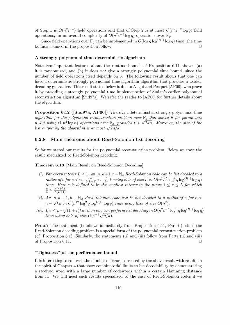
of Step 1 is O(n2ε−5) field operations and that of Step 2 is at most O(n2ε−2 log q) fieldoperations, for an overall complexity of O(n2ε−5 log q) operations over Fq.

Since field operations over Fq can be implemented in O(log q logO(1) log q) time, the timebounds claimed in the proposition follow. 2

A strongly polynomial time deterministic algorithm

Note two important features about the runtime bounds of Proposition 6.11 above: (a)it is randomized, and (b) it does not give a strongly polynomial time bound, since thenumber of field operations itself depends on q. The following result shows that one canhave a deterministic strongly polynomial time algorithm algorithm that provides a weakerdecoding guarantee. This result stated below is due to Augot and Pecquet [AP00], who proveit by providing a strongly polynomial time implementation of Sudan’s earlier polynomialreconstruction algorithm [Sud97a]. We refer the reader to [AP00] for further details aboutthe algorithm.

Proposition 6.12 ([Sud97a, AP00]) There is a deterministic, strongly polynomial timealgorithm for the polynomial reconstruction problem over Fq that solves it for parametersn, k, t using O(n2 log n) operations over Fq, provided t >

√2kn. Moreover, the size of the

list output by the algorithm is at most√

2n/k.

6.2.8 Main theorems about Reed-Solomon list decoding

So far we stated our results for the polynomial reconstruction problem. Below we state theresult specialized to Reed-Solomon decoding.

Theorem 6.13 [Main Result on Reed-Solomon Decoding]

(i) For every integer L ≥ 1, an [n, k+1, n−k]q Reed-Solomon code can be list decoded to aradius of e for e < n− r+1

2(L+1) ·n−L2r ·k using lists of size L in O(n2L5 log2 q logO(1) log q)

time. Here r is defined to be the smallest integer in the range 1 ≤ r ≤ L for whichkn ≤

r(r+1)L(L+1) .

(ii) An [n, k + 1, n − k]q Reed-Solomon code can be list decoded to a radius of e for e <n−√kn in O(n12 log2 q logO(1) log q) time using lists of size O(n2).

(iii) If e ≤ n−√

(1 + ε)kn, then one can perform list decoding in O(n2ε−5 log2 q logO(1) log q)time using lists of size O(ε−1

√n/k).

Proof: The statement (i) follows immediately from Proposition 6.11, Part (i), since theReed-Solomon decoding problem is a special form of the polynomial reconstruction problem(cf. Proposition 6.1). Similarly, the statements (ii) and (iii) follow from Parts (ii) and (iii)of Proposition 6.11. 2

“Tightness” of the performance bound

It is interesting to contrast the number of errors corrected by the above result with results inthe spirit of Chapter 4 that show combinatorial limits to list decodability by demonstratinga received word with a large number of codewords within a certain Hamming distancefrom it. We will need such results specialized to the case of Reed-Solomon codes if we

110

wish to understand the maximum number of errors for which a Reed-Solomon code canbe list decoded using lists of a certain size. Since we decode up to the Johnson radius,the performance of our algorithm will be the best possible if the Johnson bound is tightfor Reed-Solomon codes. However, we do not know this result. (Our results in Chapter 4proved the tightness of the Johnson bound for some “contrived” binary code construction,but not for Reed-Solomon codes.)

Justesen and Hφholdt [JH01] demonstrate that for certain Reed-Solomon codes, thereexist Hamming balls of radius close to (n−

√kn) with Ω(n) codewords. This provides strong

evidence to the tightness of the Johnson bound (and the number of errors corrected byour algorithm) for list decoding Reed-Solomon codes with constant-sized lists. This result,however, applies only to certain values of the rate. They also obtain results that demonstratethe tightness of the exact bound of Theorem 6.13 for list-of-L decoding for certain valuesof the rate (namely the values j(j+1)

L(L+1) for 0 ≤ j ≤ L). Ruckenstein and Roth [RR01] extendthis result to a wider range of rates — in particular, they demonstrate the tightness ofTheorem 6.13 for all values of rate in the ranges [0, 2

L(L+1) ] and [L−1L+1 , 1]. These bounds

are of interest in that they hint at a potential limitation to further improvements to thelist decoding approach, and they provide good evidence to the tightness of some of ourperformance bounds. Ruckenstein and Roth [RR01] also demonstrate that for certain settingof parameters, one cannot realize configurations exhibiting the tightness of the list-of-Ldecoding bound of Theorem 6.13, in a Reed-Solomon code. Thus a precise understandingof the combinatorics of list decoding Reed-Solomon codes is still lacking and the problemcertainly deserves further study.

6.2.9 Some Further Consequences

We now describe some other easy consequences and extensions of the polynomial reconstruc-tion algorithm of Section 6.2.3. The first three classes of results are just straightforwardapplications of the polynomial reconstruction algorithm. The fourth result, described in thenext section, revisits the curve-fitting algorithm to get a solution to a weighted polynomialreconstruction problem.

Alternant codes

We now describe a family of codes called alternant codes. Alternant codes were first definedand studied by Helgert [Hel74]. A good discussion of alternant codes appears in [MS81,Chap. 12]. Alternant codes are a very broad class of codes which among other things includeReed-Solomon codes and BCH codes. BCH codes (short for Bose-Chaudhuri-Hocquenghemcodes) are an extremely useful and well-studied family of codes, first introduced by [BR60,Hoc59] (see [MS81, Chap. 9] for a thorough discussion of BCH codes). They possess severalof the nice algebraic properties of Reed-Solomon codes, but in addition have the advantagethat codes with large blocklengths can be defined even over a fixed, small alphabet (unlikeReed-Solomon codes which require an alphabet size at least as large as the blocklength).

Definition 6.3 (Alternant Codes ([MS81], §12.2)) For positive integers m, k0, n, primepower q, the field F = GF(qm), a vector ~α of distinct elements α1, . . . , αn ∈ GF(qm), anda vector ~v of nonzero elements v1, . . . , vn ∈ GF(qm), the q-ary alternant code Aq,n,k0,~α,~v

comprises of those codewords of the Generalized Reed-Solomon code GRSF,n,k0,~α,~v that haveall components from GF(q).

111

Since the Generalized Reed-Solomon code has distance exactly n − k0 + 1, it followsthat the respective alternant code, being a subcode of the Generalized Reed-Solomon code,has distance at least n− k0 + 1. We term this the designed distance d′ = n− k0 + 1 of thealternant code. The actual rate and distance of the code are harder to determine. The ratelies somewhere between n−m(n− k0) and k0, and the distance d lies between d′ and md′.

The decoding algorithm of the previous section can be used to decode alternant codesas well. Given a received word 〈r1, . . . , rn〉 ∈ GF(q)n, we use as input to the polynomialreconstruction problem the pairs (xi, yi)ni=1, where xi = αi and yi = ri/vi are elementsof GF(qm) (here we are viewing each element ri ∈ GF(q) as an element of GF(qm)). Thelist of polynomials output includes all possible codewords from the alternant code. Thusthe decoding algorithm for the earlier section is really a decoding algorithm for alternantcodes as well, with the caveat that its performance can only be compared with the designeddistance, rather than the actual distance. The following theorem summarizes the scope ofthe decoding algorithm.

Theorem 6.14 Let A be an [n, k+1, d]q alternant code with designed distance d′ (and thussatisfying d

m ≤ d′ ≤ d). Then there exists a polynomial time list decoding algorithm for Adecoding up to e < n−

√n(n− d′) errors.

Discussion: We note that decoding algorithms for alternant codes given in classical textslike [MS81, Ber68] seem to correct only up to half the designed distance. Hence the abovetheorem improves upon those algorithms for every value of the designed distance. Sincealternant codes include BCH codes as a special case, in particular we also have an algorithmto decode BCH codes up to the above radius. However, BCH codes can be defined oversmall alphabets, even over GF(2), and then the above bound (n−

√n(n− d′)) which does

account for the alphabet size is quite far from the Johnson radius (which for binary codes

is n−√n(n−2d′)

2 , from Theorem 3.2 of Chapter 3). But as noted by [KV00] it is possibleto use the soft decoding algorithm that we will shortly discuss in Section 6.2.10 to decodeq-ary BCH codes up to the q-ary Johnson radius. A similar situation arises with algebraic-geometric codes, and in Section 6.3.8 we will discuss how to use soft decoding to decodethem up to the q-ary Johnson radius. The same argument will also apply to BCH codes, byusing the soft decoding algorithm from Theorem 6.21 instead of the soft decoding algorithmfor decoding AG-codes from Theorem 6.35.

Decoding with uncertain receptions

Consider the situation when, instead of receiving a single word y = 〈y1, y2, . . . , yn〉, for eachi ∈ [n], we receive a list of ` possibilities yi1, yi2, . . . , yi` such that one of them is the correctsymbol (but we do not know which one). Once again, as in normal list decoding, we wishto find out all possible codewords which could have been possibly transmitted, except thatnow the guarantee given to us is not in terms of the number of errors effected, but in termsof the maximum number of uncertain possibilities at each position of the received word.Let us call this problem decoding from uncertain receptions. In this situation, we have thefollowing result.

Theorem 6.15 List decoding from uncertain receptions on a [n, k + 1, d = n − k]q Reed-Solomon code can be done in polynomial time provided the number of “uncertain possibili-ties” l at each position i ∈ [n] is (strictly) less than n/k.

112

Proof: Apply the solution to the polynomial reconstruction problem with input being theset of pairs (xi, yij) : 1 ≤ i ≤ n, 1 ≤ j ≤ `, the goal being to find all degree k polynomialsp such that p(xi) ∈ yi1, . . . , yi` for every i, 1 ≤ i ≤ n. Applying Proposition 6.11, Part(ii), with the total number of pairs N = n` and t = n, we get that we can solve this problemin polynomial time provided n >

√kn`, or if ` < n/k. 2

We can also consider the situation when given lists Li of size ` at each position of thecode, we wish to find all Reed-Solomon codewords that agree with an element of the listLi for at least a fraction α of the positions i.6 The polynomial reconstruction problem stillcaptures this problem, and below we state a version of the result that follows from Part (iii)of Proposition 6.11.

Theorem 6.16 Let C be an [n, k + 1, n − k]q Reed-Solomon code. Suppose we are givenlists Li ⊆ Fq such that the average list size equals `, i.e.,

∑i |Li| = `n. Then, there are

at most O(γ−1√n`/k) codewords of C which agree with an element of Li for at least αn

values of i, provided α >√

(1 + γ)k`/n. Moreover, the list of all such codewords can befound in randomized O(n2`2γ−5 log2 q logO(1) log q) time.

We can obtain a strongly polynomial time version of the above result using the resultof Proposition 6.12. This is very useful for certain later applications where we considerReed-Solomon codes over very large alphabets (compared to the blocklength).

Theorem 6.17 Let C be an [n, k+ 1, n− k]q Reed-Solomon code of rate r. Suppose we aregiven lists Li ⊆ Fq such that the average list size equals `, i.e.,

∑i |Li| = `n. Then, there are

at most√

2n`/k codewords of C which agree with an element of Li for at least αn values ofi, provided α >

√2k`/n. Moreover, the list of all such codewords can be found deterministi-

cally using O(n2`2r−O(1) log(n`)) operations over Fq, or in O(n2`2r−O(1) log(n`) log q logO(1) log q)time. (For constant rate, the runtime equals O((n`)2 log(n`) log q logO(1) log q).)

The above versions of the result and the soft decoding algorithm from Proposition 6.21to be discussed shortly are in fact the main forms of our decoding results for Reed-Solomoncodes that will be used repeatedly in later chapters.

Errors and Erasures decoding

The algorithm of Section 6.2.3 is also capable of dealing with other notions of corruptionof information. A much weaker notion of corruption than an error in data transmissionis that of an “erasure”. Here a transmitted symbol is either simply “lost” or receivedin obviously corrupted shape (so we might as well declare it erased). We now note thatthe decoding algorithm of Section 6.2.3 naturally handles the case when there are botherrors and erasures. Suppose n symbols were transmitted and n′ ≤ n were received ands = n − n′ symbols got erased. (We stress that the problem definition specifies that thereceiver knows which symbols are erased.) This problem just reduces to a polynomialreconstruction problem on n′ points. An application of Proposition 6.11 yields that e errorscan be corrected provided e < n′ −

√n′k. Thus we get:

6This model of decoding will be formally defined and called list recovering in Chapter 9, where we willstudy combinatorial aspects of codes with good list recoverability, and will also make use of the list recoveringproperty of Reed-Solomon codes.

113

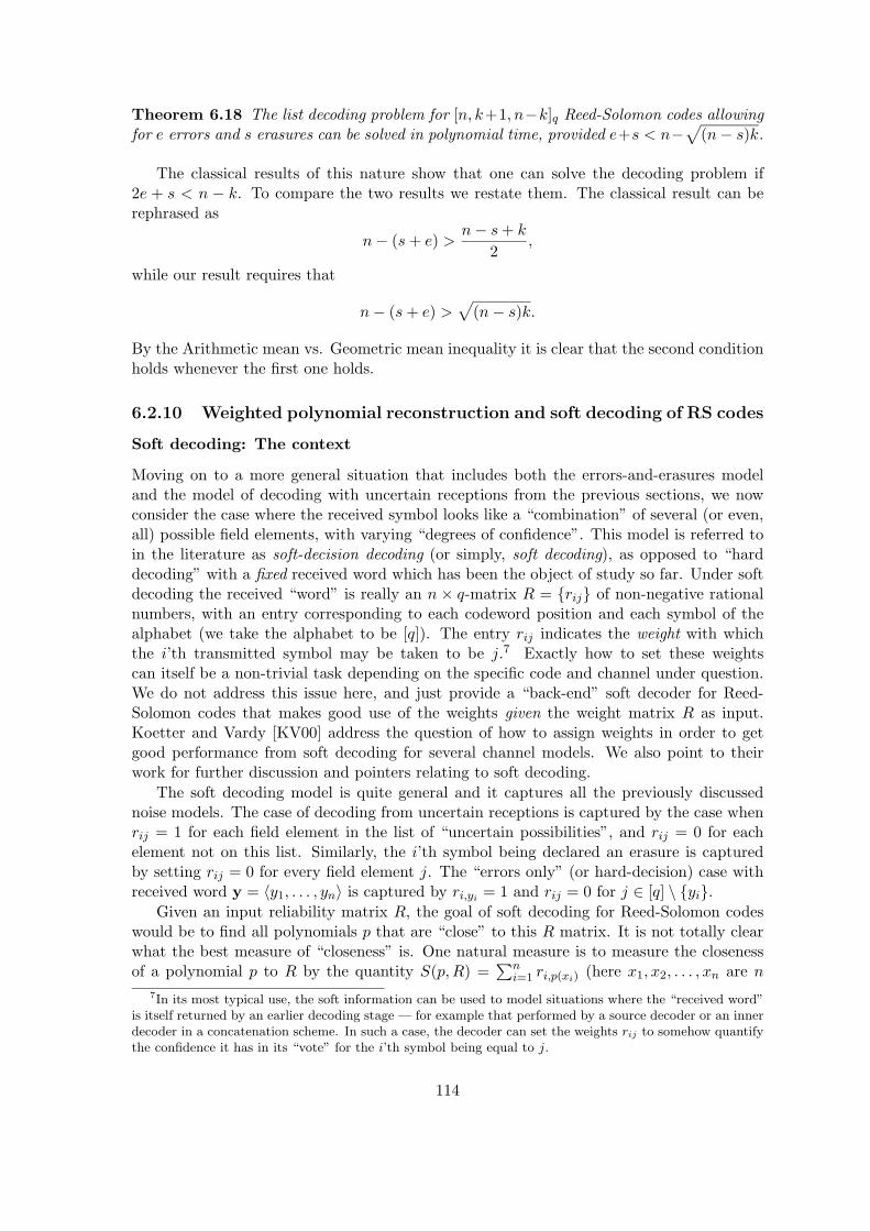
Theorem 6.18 The list decoding problem for [n, k+1, n−k]q Reed-Solomon codes allowingfor e errors and s erasures can be solved in polynomial time, provided e+s < n−

√(n− s)k.

The classical results of this nature show that one can solve the decoding problem if2e + s < n − k. To compare the two results we restate them. The classical result can berephrased as

n− (s+ e) >n− s+ k

2,

while our result requires that

n− (s+ e) >√

(n− s)k.

By the Arithmetic mean vs. Geometric mean inequality it is clear that the second conditionholds whenever the first one holds.

6.2.10 Weighted polynomial reconstruction and soft decoding of RS codes

Soft decoding: The context

Moving on to a more general situation that includes both the errors-and-erasures modeland the model of decoding with uncertain receptions from the previous sections, we nowconsider the case where the received symbol looks like a “combination” of several (or even,all) possible field elements, with varying “degrees of confidence”. This model is referred toin the literature as soft-decision decoding (or simply, soft decoding), as opposed to “harddecoding” with a fixed received word which has been the object of study so far. Under softdecoding the received “word” is really an n × q-matrix R = rij of non-negative rationalnumbers, with an entry corresponding to each codeword position and each symbol of thealphabet (we take the alphabet to be [q]). The entry rij indicates the weight with whichthe i’th transmitted symbol may be taken to be j.7 Exactly how to set these weightscan itself be a non-trivial task depending on the specific code and channel under question.We do not address this issue here, and just provide a “back-end” soft decoder for Reed-Solomon codes that makes good use of the weights given the weight matrix R as input.Koetter and Vardy [KV00] address the question of how to assign weights in order to getgood performance from soft decoding for several channel models. We also point to theirwork for further discussion and pointers relating to soft decoding.

The soft decoding model is quite general and it captures all the previously discussednoise models. The case of decoding from uncertain receptions is captured by the case whenrij = 1 for each field element in the list of “uncertain possibilities”, and rij = 0 for eachelement not on this list. Similarly, the i’th symbol being declared an erasure is capturedby setting rij = 0 for every field element j. The “errors only” (or hard-decision) case withreceived word y = 〈y1, . . . , yn〉 is captured by ri,yi = 1 and rij = 0 for j ∈ [q] \ yi.

Given an input reliability matrix R, the goal of soft decoding for Reed-Solomon codeswould be to find all polynomials p that are “close” to this R matrix. It is not totally clearwhat the best measure of “closeness” is. One natural measure is to measure the closenessof a polynomial p to R by the quantity S(p,R) =

∑ni=1 ri,p(xi) (here x1, x2, . . . , xn are n

7In its most typical use, the soft information can be used to model situations where the “received word”is itself returned by an earlier decoding stage — for example that performed by a source decoder or an innerdecoder in a concatenation scheme. In such a case, the decoder can set the weights rij to somehow quantifythe confidence it has in its “vote” for the i’th symbol being equal to j.

114

distinct field elements that define the Reed-Solomon encoding of a polynomial p). The holygrail in this setting is maximum likelihood soft-decision decoding, where the goal is to findthe polynomial p that maximizes S(p,R). This turns out to be a prohibitively difficultalgorithmic task, so one studies the bounded distance soft decoding problem. This problemreduces to the problem of finding a list of all polynomials p such that S(p,R) is at least acertain threshold.

In what follows, we provide a polynomial time bounded distance soft decoding algorithmfor Reed-Solomon codes. For a matrix R as input, the algorithm finds all degree k poly-nomials p such that S(p,R) is at least

√k times the L2 norm of the R matrix. We obtain

our soft decoding algorithm via a solution to a weighted generalization of the polynomialreconstruction problem, which we define next.

Weighted polynomial reconstruction

We first formally define the problem.

Problem 3 (Weighted polynomial reconstruction)Input: N distinct pairs (x1, y1), . . . , (xN , yN ), where each xi, yi ∈ F for some field F;N non-negative weights w1, . . . , wN ;degree parameter k and agreement parameter W .Output: All polynomials p of degree at most k which satisfy∑

i:p(xi)=yi

wi ≥W .

Note: There is no requirement of distinctness on the various xi’s in the above specification.This will be crucial to the application to soft decoding algorithms for Reed-Solomon codes.

We now discuss how the algorithm Poly-Reconstruct can be modified to solve the weightedpolynomial reconstruction problem for the case when the weights are non-negative integers.The basic idea is to use multiplicities at the various points (xi, yi) in proportion to theirweights, in the interpolation step (Step 1 of the algorithm). Specifically, in Step 1, wewould find a polynomial Q which has a singularity of order wiρ at the point (xi, yi), for asuitably large integer parameter ρ. Thus we would now have

∑ni=1

(ρwi+1

2

)constraints. If

a polynomial p passes through the points (xi, yi) for every i ∈ S for some S ⊆ [n], theny−p(x) will appear as a factor ofQ(x, y) provided

∑i∈S ρwi is greater than (1, k)-wt-deg(Q).

Also (1, k)-wt-deg(Q) must be picked large enough such that Q has more coefficients thanthe number of linear constraints it must satisfy (so that a non-zero Q with the requiredproperties will be guaranteed to exist). Optimizing over the weighted degree of Q yieldsthe following theorem – the proof is similar to Theorem 6.8.

Theorem 6.19 If the weights wi are non-negative integers, the weighted polynomial re-construction problem with parameters k,W over Fq can be solved deterministically in time

polynomial in the sum of wi’s and q, provided W >√k∑N

i=1w2i .

We now remove the requirement of integer weights and the pseudo-polynomial depen-dence of the runtime on the wi’s (ideally we would like the algorithm to run in time polyno-mial in the logarithm of the wi’s). Below we note that with an ε degradation in performance,the algorithm can be implemented to run in poly(N, 1/ε) time, even when the weights arearbitrary rational numbers.

115

Lemma 6.20 For any tolerance parameter ε > 0, the weighted polynomial reconstructionproblem for N pairs (xi, yi) ∈ F2

q with associated non-negative rational weights wi, degreeparameter k and agreement parameter W , can be solved deterministically in time polynomialin N , q and 1/ε, provided

W >

√√√√k

N∑i=1

w2i + εwmax.

Proof: Assume without loss of generality that w1 ≤ w2 ≤ · · · ≤ wN . Pick any large integerL ≥ N

ε , and form the integer weights w′i = bLwi/wNc. Since wi ≤ wN for all i, the weightsw′i are all at most L. Therefore Theorem 6.19 implies that one can find, in poly(N,L) time,a list of all polynomials p of degree less at most k that satisfy

∑i:p(xi)=yi

w′i >

√√√√kN∑i=1

w′2i .

But since Lwi/wN ≥ w′i > Lwi/wN − 1, this implies that in poly(N,L, q) = poly(N, q, 1/ε)time, we can find all polynomials p of degree at most k that satisfy the condition

∑i:p(xi)=yi

(LwiwN− 1)≥

√√√√kN∑i=1

(LwiwN

)2

⇐=∑

i:p(xi)=yi

wi ≥

√√√√kN∑i=1

w2i +

NwNL

⇐=∑

i:p(xi)=yi

wi ≥

√√√√kN∑i=1

w2i + εwN

(the last step follows since L ≥ N/ε). 2

Reed-Solomon soft decoding: Main result

We also record the following consequence for soft decoding of Reed-Solomon codes. Its prooffollows immediately from the above lemma. We will appeal to this result several times whenwe discuss decoding algorithms for concatenated codes in Chapter 8 of the thesis.

Theorem 6.21 (Soft list decoding of Reed-Solomon codes) Consider an [n, k+1, n−k]q Reed-Solomon code with messages being polynomials r over Fq of degree at most k. Letthe encoding function be r 7→ 〈r(x1), r(x2), . . . , r(xn)〉 where x1, . . . , xn are distinct ele-ments of Fq. Let ε > 0 be an arbitrary constant. For each i ∈ [n] and α ∈ Fq, let wi,α bea non-negative rational number. Then, there exists a deterministic algorithm with runtimepoly(n, q, 1/ε) that, when given as input the weights wi,α for i ∈ [n] and α ∈ Fq, finds a listof all polynomials p ∈ Fq[x] of degree at most k that satisfy

n∑i=1

wi,p(xi) ≥

√√√√k

n∑i=1

∑α∈Fq

w2i,α + εmax

i,αwi,α . (6.12)

Finally, we would like to point out that, once again, the error-correction performance ofthe above result approaches what is indicated to be possible by the combinatorial bounds onlist decodability, specifically the “weighted Johnson bound” from Corollary 3.7 of Chapter 3.

116

Significance of weighted polynomial reconstruction

The weighted polynomial reconstruction problem is at the heart of soft decoding algorithmsfor Reed-Solomon codes (cf. [KV00]). It also plays a crucial role in decoding certainconcatenated codes, where the weights for Reed-Solomon decoding are passed by the innerdecoder [GS00, Nie00, GHSZ00, Gur01b]. This will be discussed in detail in Chapter 8on concatenated codes. Thus, the weighted polynomial reconstruction is a very usefulsubroutine that has found several applications to list decoding, and we view it as one of thekey contributions of this thesis.

Also, the basic algebraic technique behind weighted polynomial reconstruction extendsto more general codes than Reed-Solomon codes. In the next section, we will present a listdecoding algorithm for algebraic-geometric codes, which then also generalizes to a weightedversion (Section 6.3.7). In the next chapter, we will present a soft list decoding algorithmfor an even broader class of codes called “ideal-based” codes.

6.3 Algebraic-Geometric Codes

We now describe the extension of our algorithm to the case of algebraic-geometric codes.Our extension shows that the algebra of the previous section extends to the case of algebraicfunction fields, yielding an approach to the list decoding problem for algebraic-geometriccodes. In particular it reduces the decoding problem to some basis computations in analgebraic function field and to a root-finding problem over the algebraic function field.However neither of these tasks is known to be solvable efficiently given only the generatormatrix of the algebraic-geometric code (or some such standard “minimal” representation ofa linear code). But we will show that by precomputing a polynomial amount of additionalinformation about the linear code and the underlying algebraic structures, one can solveboth parts efficiently.

6.3.1 Overview

Algebraic-geometric codes (henceforth AG-codes) are defined by evaluations of “regular”functions at a set of points on a “nice” algebraic curve. These were first defined byGoppa [Gop81] in a seminal work, and are hence sometimes also referred to as geomet-ric Goppa codes. Their properties are proved using some deep facts from the theory ofalgebraic function fields. Before we describe the generalization of the Reed-Solomon decod-ing algorithm to AG-codes, in Section 6.3.2 we first develop the necessary definitions andpreliminaries on algebraic function fields, and formally define algebraic-geometric codes.

We then present our algorithm for list decoding modulo some algorithmic assumptionsabout the underlying structures. Under these assumptions, our algorithm yields an al-gorithm for list decoding which corrects up to e < n −

√n(n− d∗) errors in a code of

blocklength n and designed distance d∗. (The earlier best result for list decoding AG-codes,due to [SW99], could correct up to about n−

√2n(n− d∗) errors.)

Obtaining an efficient implementation of our decoding algorithm raises some funda-mental questions about how elements of an algebraic function field are represented andmanipulated. We next discuss these issues in detail and demonstrate a representation ofAG-codes under which the list decoding algorithm can be implemented to run in polynomialtime. This turns out to be a non-standard representation (i.e., we do not how to implementthe algorithm in polynomial time given only the generator matrix or some such “standard”

117

representation of the code). However, the necessary representation of the code is succinctand is of size polynomial in the blocklength of the code.

6.3.2 Algebraic-geometric codes: Preliminaries

We now discuss the main notions associated with the theory of algebraic function fieldsthat will be necessary for defining and studying algebraic-geometric codes. The interestedreader may find further details in [Sti93, GS95a]. In the presentation below, we will assumefamiliarity with the basic notions of field extensions, which can be found in any standardalgebra text, eg., [Art91]. We note that the definition of AG-codes presented here is inline with that of the standard texts (in particular, we closely follow the presentation inStichtenoth’s book [Sti93]) — a different presentation which is somewhat less heavy onalgebraic terminology appears in the paper by the author and Sudan [GS99] where thedecoding algorithm discussed here first appeared.

An extension field K of a field k, denoted K/k, is an algebraic function field (or simply,function field) over k if the following conditions are satisfied: (i) There is an element x ∈K that is transcendental over k such that K is a finite extension of k(x), and (ii) k isalgebraically closed in K, that is, the only elements in K that are algebraic over k are thosein k.

For our applications to AG-codes, we will be interested in the case when k is a finitefield, i.e., k = Fq for some prime power q. A function field K/Fq can be obtained as K =Fq(X)[y1, y2, . . . , ym] where each yi satisfies some polynomial equation over Fq(X)[y1, . . . , yi−1].For the rest of this section, K will denote the function field in question.

Places and Valuations: A function field K/Fq has a set of places PK and the associatedset of valuations, given by a valuation map v : PK ×K → Z ∪ ∞. The exact definitionof these notions can be found, for instance, in [Sti93]; we only abstract some propertiesrelevant to us below.

Intuitively the places correspond to “points” on the algebraic curve associated with thefunction field K, and the valuation map tells us how many poles or zeroes a function in Khas at a specific place in PK . It has the property that for any f ∈ K, there are only finitelymany places P ∈ PK such that v(P, f) 6= 0. As is normal practice, for each P ∈ PK , wedenote by vP : K → Z∪∞, the map vP (·) = v(P, ·) which tells how many zeroes or polesa given function has at P (with the convention vP (0) =∞ for any place P ). If vP (x) < 0,we say x has a pole at P , and −vP (x) is called the pole order of x at P . Similarly, ifvP (x) > 0, we say that x has a zero at P , and in such a case vP (x) is the zero order of x atP . The valuation vP at any place satisfies the following properties:

(a) vP (a) =∞ iff a = 0 and vP (a) = 0 for all a ∈ Fq \ 0.

(b) vP (ab) = vP (a) + vP (b) for all a, b ∈ K \ 0.

(c) vP (a+ b) ≥ minvP (a), vP (b) for all a, b ∈ K.

For those familiar with some commutative algebra terminology, we just recap how placesare formally defined from their corresponding valuations. For every valuation vP of K, thering of regular functions at P , denoted OP , is defined to be

OP = x ∈ K : vP (x) ≥ 0 .

118

This ring is a “discrete valuation ring” and in particular is a local ring with a uniquemaximal ideal. This unique maximal ideal of OP is defined to be the “place” P associatedwith vP , and is given by

P = x ∈ K : vP (x) > 0 .

Intuitively, OP is the ring of functions in K that do not have any poles at a certain “point”on the curve; the place P corresponds to this point, and is algebraically defined as the idealof functions in K that vanish at that “point”.

Degree of a place: Associated with every place is a degree abstracted via the map deg :PK → Z

+. The degree, deg(P ), of any place P is a positive integer and intuitively meansthe following: when we pick a function f ∈ K which has no poles at P and “evaluate” itat P , we get a value in the field Fqdeg(P ) . Places of degree one correspond to rational pointson the curve. More formally, the notion of degree means the following: for every place P ,the quotient ring OP /P is a finite field of size qdeg(P ).

Evaluations of functions at places: We can abstract the notion of evaluation of elementsof the function field at the places by a map eval : K × PK → Fq ∪ ∞ (here Fq =

⋃i≥1 Fqi

is the algebraic closure of Fq). This map has the following properties:

(i) For every P ∈ PK and f ∈ K, eval(f, P ) = ∞ iff vP (f) < 0, and eval(f, P ) = 0 iffvP (f) > 0.

(ii) If f ∈ K, P ∈ PK and vP (f) ≥ 0, then eval(f, P ) ∈ Fqdeg(P ) .

(iii) The map eval respects field operations; in other words, if vP (f1) ≥ 0 and vP (f2) ≥ 0,then eval(f1 + f2, P ) = eval(f1, P ) + eval(f2, P ), and eval(f1 ∗ f2, P ) = eval(f1, P ) ∗eval(f2, P ) (where we have used (+, ∗) to denote the addition and multiplication op-erations in both K and Fq).

Divisors: The divisor group DK of the function field K is a free abelian group on PK . Anelement D of DK is thus represented by the formal sum

∑P∈PK aPP where each aP ∈ Z,

and aP = 0 for all but finitely many P . We say D 0 if aP ≥ 0 for all P ∈ PK . Thesupport of a divisor D, denoted supp(D), is the (finite) set P ∈ PK : aP 6= 0. Thedegree map extends naturally to the divisor group DK and deg : DK → Z is defined asdeg(

∑P aPP ) =

∑P aP deg(P ).

For every f ∈ K \ 0, there is an associated divisor, called the principal divisor anddenoted (f), which is defined by (f) =

∑P vP (f)P . The following result states that degree

of any principal divisor equals 0. It is a well-known result and just states that every non-zerofunction in the function field has an equal number of zeroes and poles.

Proposition 6.22 For any function field K/Fq and any f ∈ K \ 0, deg((f)) = 0.

The Riemann-Roch Theorem: For every divisor D ∈ DK , one can define the linearspace of functions L(D) as

L(D) = g ∈ K : (g) +D 0.

For example for a divisor D = aQ − bP where P,Q ∈ PK and a, b > 0, L(D) is thespace of all functions that have at least b zeroes at P and at most a poles at Q. It isknown that for any divisor D 0, L(D) is a finite-dimensional vector space over Fq and

119

dim(L(D)) ≤ 1 + deg(D) (see [Sti93] for a proof). A lower bound on dim(L(D)) is givenby the celebrated Riemann-Roch theorem for function fields, which is stated below. Thetheorem statement also introduces the “genus” of a function field K/Fq, which in somesense measures the “complexity” of the underlying algebraic curve. (A genus equal to zerocorresponds to the simplest case when K = Fq(X) is the field of all rational functions inone variable.)

Theorem 6.23 [Riemann-Roch]: Let K/Fq be any function field. There is a non-negative integer g, called the genus of K/Fq, such that

(a) For any divisor D ∈ DK , dim(L(D)) ≥ deg(D)− g + 1.

(b) There is an integer c, depending only on K/Fq, such that dim(L(D)) = deg(D)−g+1whenever deg(D) ≥ c. Furthermore, c ≤ 2g − 1.

Algebraic-geometric codes: We are now ready to define the notion of an AG-code (alsoknown as geometric Goppa code). Let K/Fq be an algebraic function field of genus g, letP0, P1, P2, . . . , Pn be distinct places of degree one in PK , and let G = P1 +P2 + · · ·+Pn andD = αP0 be divisors of K/Fq (note that supp(G) ∩ supp(D) = ∅).

The algebraic-geometric code CL(G,D) = CL(G,α, P0) is defined by

CL(G,α, P0) := (eval(f, P1), . . . , eval(f, Pn)) : f ∈ L(αP0) ⊆ Fnq .

(Note that eval(f, Pi) ∈ Fq since vPi(f) ≥ 0 and deg(Pi) = 1.) It is clear that the definedspace is a linear space, since L(αP0) is an Fq-linear vector space. The following Propositionfollows from the Riemann-Roch theorem and quantifies the parameters of these codes. 8

Proposition 6.24 Let K/Fq be a function field of genus g, and let α, n be positive integerswith α < n. Let P0, P1, P2, . . . , Pn be distinct places of degree one in PK , and let G bethe divisor G = P1 + P2 + . . . + Pn. Then CL(G,α, P0) is an [n, k, d]q code with k =

dim(L(αP0)) ≥ α − g + 1 and d ≥ d∗def= n − α. The quantity d∗ = n − α is called the

designed distance of the code. Moreover, if α ≥ 2g − 1, then k = α− g + 1.

Proof: The claims about the dimension follow from the Riemann-Roch theorem. For thedistance property, let f1 6= f2 ∈ L(αP0) be two distinct messages of CL(G,α, P0). Thenf1 − f2 ∈ L(αP0) as well, and hence f1 − f2 has at most α deg(P0) = α poles in all. ByProposition 6.22, f1 − f2 has at most α zeroes, and hence eval(f1 − f2, Pi) = 0 for at mostα values of i, 1 ≤ i ≤ n. Therefore, the encodings of f1 and f2 agree on at most α placesamong P1, P2, . . . , Pn, which proves that the distance of the code is at least n− α. 2

Significance of AG-codes: Codes constructed as above and achieving d/n, k/n > 0 (in thelimit of large n) are known for constant alphabet size q. In fact, such codes achieving boundsbetter than those known by probabilistic constructions are known for q ≥ 49 [TVZ82]. Sucha situation, where an explicit construction is better than the best probabilistic construction,

8The AG-codes defined here are the so called “one-point divisor codes” since the space of functions areallowed to have poles at only one place. While one can also study AG-codes defined using more generaldivisors (i.e., allow poles at multiple places), one-point divisor codes are the most widely studied AG-codes,and there is no clear quantitative advantage of using more general divisors in defining the code. Therefore, inthis thesis we will focus only on one-point divisor codes. An explicit generalization of the decoding algorithmpresented in this thesis to the case of AG-codes based on general divisors appears, for instance, in [Pec01].

120

is quite rare in combinatorics. This is one of the primary reasons for the importance ofand enormous interest in algebraic-geometric codes. Moreover, AG-codes have a very richalgebraic structure which can be exploited to design efficient decoding algorithms, as we doin this section. Recently, Elkies [Elk01] defined a more general algebraic family of codes thanthe AG-codes discussed here. His codes are non-linear and are based on some deep algebraicproperties of certain modular curves. For certain setting of parameters his codes provide anasymptotic improvement over what is possible using “conventional” AG-codes. Thus theunderlying idea of defining codes by evaluations of “nice” functions on a suitably pickedset of points on a “nice” algebraic curve or variety is a very powerful one. Our decodingalgorithm gives a powerful and quite general method of dealing with such algebraic codes.

6.3.3 List decoding algorithm for algebraic-geometric codes

We now describe the extension of our Reed-Solomon list decoding algorithm to the caseof algebraic-geometric codes. We begin with a formal description of the problem – this isthe generalization of the polynomial reconstruction problem discussed in the decoding ofReed-Solomon codes to the case of algebraic function fields.

Problem 4 (Function Reconstruction)Input: Integers n, α, t; n distinct pairs (Pi, yi)ni=1 where each Pi is a place of degreeone of the function field K/Fq, and each yi ∈ Fq; and a place P0 of degree one with P0 /∈P1, . . . , Pn.Output: All functions h in L(αP0) that satisfy eval(h, Pi) = yi for at least t values of i,1 ≤ i ≤ n.

As before, it is easily seen the list decoding problem for the AG-code CL(G,α, P0) from(n − t) errors (with divisor G = P1 + P2 + . . . + Pn) reduces to the above reconstructionproblem. While in the AG-codes case the places Pi are distinct, note that this is not requiredin the above specification, and indeed as with the case of polynomial reconstruction, we willsolve the above problem without assuming that the Pi’s are distinct.

Solution Idea

As with the Reed-Solomon case, we will first try to describe the data points (Pi, yi) bysome polynomial Q. We follow [SW99] and let Q be a polynomial in a formal variable ywith coefficients from K (i.e., Q ∈ K[y]). Now given a value of yi ∈ Fq, Q(yi) will yield anelement of K. By definition such an element of K can be evaluated at the place Pi ∈ PK .We will require that Q have the property that Q(Pi, yi)

def= eval(Q(yi), Pi) equal zero, forevery i ∈ [n]. We will actually require more and insist that (Pi, yi) “behave” like a zeroof multiplicity r of Q; since Pi ∈ PK and yi ∈ Fq, we need to be careful in specifying theconditions to achieve this, and we will return to this shortly. We will also insist that Q(y)has a small number of poles (say, at most l) at P0 for any substitution of y with a functionin L(αP0). Having found such a Q, we then look for roots h ∈ L(αP0) of Q, and winnowout those that do not satisfy eval(h, Pi) = yi for at least t values of i, 1 ≤ i ≤ n.

Description of the algorithm

Algorithm Function-Reconstruct(n, α, t;P0, P1, . . . , Pn ∈ PK)Input: y1, y2, . . . , yn ∈ Fq

121

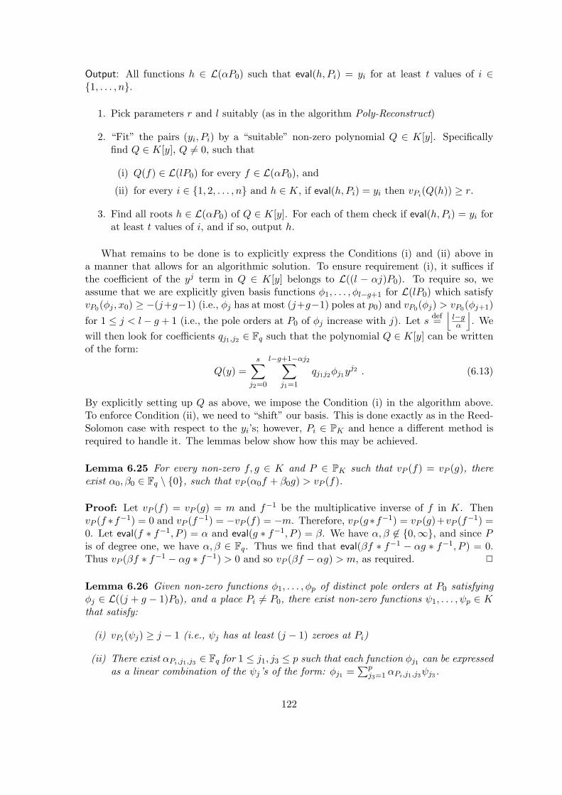
Output: All functions h ∈ L(αP0) such that eval(h, Pi) = yi for at least t values of i ∈1, . . . , n.

1. Pick parameters r and l suitably (as in the algorithm Poly-Reconstruct)

2. “Fit” the pairs (yi, Pi) by a “suitable” non-zero polynomial Q ∈ K[y]. Specificallyfind Q ∈ K[y], Q 6= 0, such that

(i) Q(f) ∈ L(lP0) for every f ∈ L(αP0), and

(ii) for every i ∈ 1, 2, . . . , n and h ∈ K, if eval(h, Pi) = yi then vPi(Q(h)) ≥ r.

3. Find all roots h ∈ L(αP0) of Q ∈ K[y]. For each of them check if eval(h, Pi) = yi forat least t values of i, and if so, output h.

What remains to be done is to explicitly express the Conditions (i) and (ii) above ina manner that allows for an algorithmic solution. To ensure requirement (i), it suffices ifthe coefficient of the yj term in Q ∈ K[y] belongs to L((l − αj)P0). To require so, weassume that we are explicitly given basis functions φ1, . . . , φl−g+1 for L(lP0) which satisfyvP0(φj , x0) ≥ −(j+g−1) (i.e., φj has at most (j+g−1) poles at p0) and vP0(φj) > vP0(φj+1)

for 1 ≤ j < l − g + 1 (i.e., the pole orders at P0 of φj increase with j). Let s def=⌊l−gα

⌋. We

will then look for coefficients qj1,j2 ∈ Fq such that the polynomial Q ∈ K[y] can be writtenof the form:

Q(y) =s∑

j2=0

l−g+1−αj2∑j1=1

qj1j2φj1yj2 . (6.13)

By explicitly setting up Q as above, we impose the Condition (i) in the algorithm above.To enforce Condition (ii), we need to “shift” our basis. This is done exactly as in the Reed-Solomon case with respect to the yi’s; however, Pi ∈ PK and hence a different method isrequired to handle it. The lemmas below show how this may be achieved.

Lemma 6.25 For every non-zero f, g ∈ K and P ∈ PK such that vP (f) = vP (g), thereexist α0, β0 ∈ Fq \ 0, such that vP (α0f + β0g) > vP (f).

Proof: Let vP (f) = vP (g) = m and f−1 be the multiplicative inverse of f in K. ThenvP (f ∗f−1) = 0 and vP (f−1) = −vP (f) = −m. Therefore, vP (g∗f−1) = vP (g)+vP (f−1) =0. Let eval(f ∗ f−1, P ) = α and eval(g ∗ f−1, P ) = β. We have α, β 6∈ 0,∞, and since Pis of degree one, we have α, β ∈ Fq. Thus we find that eval(βf ∗ f−1 − αg ∗ f−1, P ) = 0.Thus vP (βf ∗ f−1 − αg ∗ f−1) > 0 and so vP (βf − αg) > m, as required. 2

Lemma 6.26 Given non-zero functions φ1, . . . , φp of distinct pole orders at P0 satisfyingφj ∈ L((j + g − 1)P0), and a place Pi 6= P0, there exist non-zero functions ψ1, . . . , ψp ∈ Kthat satisfy:

(i) vPi(ψj) ≥ j − 1 (i.e., ψj has at least (j − 1) zeroes at Pi)

(ii) There exist αPi,j1,j3 ∈ Fq for 1 ≤ j1, j3 ≤ p such that each function φj1 can be expressedas a linear combination of the ψj’s of the form: φj1 =

∑pj3=1 αPi,j1,j3ψj3.

122

Proof: We prove a stronger statement by induction on p: If φ1, . . . , φp are linearly indepen-dent functions (over Fq) that satisfy vPi(φj) ≥ m for each j = 1, 2, . . . , p for some m ≥ 0,then there exist functions ψ1, . . . , ψp with vPi(ψj) ≥ (m+ j− 1) that generate the φj ’s overFq. Note that this will imply our lemma since the fact that φj ’s have distinct pole ordersat P0 implies that φ1, φ2, . . . , φp are linearly independent (this follows easily using the factthat vP0(αf + βg) = minvP0(f), vP0(g) if vP0(f) 6= vP0(g)).

The statement claimed is obviously true for p = 1, with the choice ψ1 = φ1. Now letp > 1. Assume without loss of generality that φ1 is a function with the least zero orderat Pi. By assumption, φ1 has at least m zeroes at Pi, i.e., vPi(φ1) ≥ m. We let ψ1 = φ1.Now, for 2 ≤ j ≤ p, set φ′j = φj if vPi(φj) > vPi(φ1). Otherwise, if vPi(φj) = vPi(φ1),using Lemma 6.25 to the pair (φ1, φj) of functions, we get αj , βj ∈ Fq − 0 such that thefunction φ′j = αjφ1 + βjφj satisfies vPi(φ

′j) > vPi(φ1) ≥ m. Since φj = β−1

j φ′j − αjβ−1j φ1

in this case, we conclude that in any case, for 2 ≤ j ≤ p, ψ1 = φ1 and φ′j generate φj .Now φ′2, φ

′3, . . . , φ

′p are linearly independent (since φ1, φ2, . . . , φp are) and vPi(φ

′j) ≥ m + 1

for 2 ≤ j ≤ p. Therefore the induction hypothesis applied to the functions φ′2, . . . , φ′p now

yields ψ2, . . . , ψp as required. 2

We are now ready to express Condition (ii) of Algorithm Function-Reconstruct whichrequires that

vPi(Q(h)) ≥ r for all h ∈ K and i ∈ 1, 2, . . . , n such that eval(h, Pi) = yi . (6.14)

Informally, we say that the above requirement forces (Pi, yi) to be a “zero” of multiplicityr of the polynomial Q. Using Lemma 6.26 and Equation (6.13), we know that Q has theform

Q(y) =s∑

j2=0

l−g+1∑j3=1

l−g+1−j2α∑j1=1

qj1,j2αPi,j1,j3 ψj3,Pi yj2 .

The shifting to yi is achieved by defining

Q(i)(y) def= Q(y + yi) . (6.15)

The requirement (6.14) on Q,Pi now becomes

vPi(Q(i)(h)) ≥ r for all h ∈ K such that eval(h, Pi) = 0, i.e., ∀ h s.t. vPi(h) ≥ 1 . (6.16)

Now

Q(i)(y) =s∑

j4=0

l−g+1∑j3=1

q(i)j3,j4

ψj3,Piyj4 , (6.17)

where

q(i)j3,j4

def=s∑

j2=j4

l−g+1−αj2∑j1=1

(j2j4

)yj2−j4i · qj1,j2αPi,j1,j3 . (6.18)

The terms in Q(i)(y) that are divisible by yp contribute p towards the multiplicity of (Pi, 0)as a “zero” of Q(i), or, equivalently, the multiplicity of (Pi, yi) as a zero of Q. SincevPi(ψj3,Pi) ≥ (j3−1) by Lemma 6.26, we can achieve the required Condition (6.16) on Q(i),or equivalently the required Condition (6.14) on Q, by insisting that q(i)

j3,j4= 0 for all j3 ≥ 1,

j4 ≥ 0 such that j4 + j3 − 1 < r, i.e. j3 + j4 ≤ r (there are(r+1

2

)such constraints for each

i ∈ 1, 2, . . . , n).

123

The above discussion shows that it is possible to solve Step 1 in Algorithm Function-Reconstruct by finding a non-zero solution to a homogeneous linear system (with unknownsbeing the coefficients qj1,j2 from the expansion (6.13) of the polynomial Q), modulo theassumption that we “know” a certain basis φ1, φ2, . . . , φl−g+1 of L(lP0), and also the “basischange coefficients” αPi,j1,j3 (from Lemma 6.26). The coefficients of the polynomial will alsobe found and expressed in terms of their representation in terms of the basis 〈φ1, . . . , φl−g+1〉.To solve Step 2, we need a subroutine to find roots of univariate polynomials over functionfields, to which we turn next.

6.3.4 Root finding over algebraic function fields

Before discussing the root finding algorithm, we discuss some issues concerning the repre-sentation of elements of a function field that deserve attention at this point. The decodingalgorithm discussed above relies strongly on the algebraic properties of the underlying func-tion field. In particular, it relies on the ability to perform certain operations over thesefields. These operations include basic field operations such as addition and multiplication,but also some non-trivial operations such as evaluating functions at “places”, and findingroots of polynomials over these fields.

One of the essential bottlenecks towards the unified presentation of our algorithm forall AG-codes is that one needs a generic method to represent the elements of an algebraicfunction field so that (a) these representations are short for the elements of interest in theconstruction of the algebraic-geometric codes; and (b) basic operations are efficient underthis representation. By carefully picking the representation of the algebraic-geometric code,we are able to meet both the requirements above. By doing so, we are able to present acompact and general theorem about list decoding of AG-codes.

As mentioned earlier, algorithms that involve function fields, and in particular decodingalgorithms for AG-codes, raise several issues on how to represent elements from the functionfield K and the places PK .

In order to implement Algorithm Function-Reconstruct efficiently over a function fieldK, we would like to perform the following basic operations efficiently: (i) Given two elementsx, y ∈ K, compute their sum and product in K; (ii) Given f ∈ K and P ∈ PK , computevP (f) and eval(f, P ); and (iii) Given a divisor D 0, compute a basis for the vector spaceL(D) over Fq (it suffices to solve this for one-point divisors D = αP0).

It is a priori unclear that these operations can performed in polynomial time for everyfunction field K. First of all, the function field K is an infinite set, so one cannot assumethat operations in K (like sum and product) are unit operations. Instead one must fix arepresentation for the elements and give explicit algorithms to perform these operationsthat are efficient with respect to the size of the representation of an element. A naturalrepresentation to consider is to express elements of K as ratio of two homogeneous multi-variate polynomials. For this representation, the field operations in K can be done in timepolynomial in the sum of degrees of the respective polynomials. However, for question (iii)above, it is not known whether for general function fields there always exists a basis forL(D) over Fq with a succinct representation (i.e., one of size polynomial in deg(D)) as theratio of polynomials (see [SW99] for a discussion concerning this point).

For applications to decoding, one does not need to work with all of K, but instead canfocus attention only on elements in L(D) for some divisor D 0 (in fact for D = lP0

for some place P0). This allows us the option of representing elements of L(D) as vectorsin Fdim(L(D))

q which represent their coordinates with respect to some fixed basis of L(D)

124

over Fq. Since it is known that dim(L(D)) ≤ deg(D) + 1, this representation will be smallprovided deg(D) is small. Indeed, this is what we exploited already in our “solution” toStep 1 of Algorithm Function-Reconstruct. In order to be able to perform the root-findingstep also efficiently, we augment this representation suitably. Before explaining this, weformally describe the basic root-finding task that we wish to solve, and describe an algebraicalgorithm to solve it (this is along the lines of the algorithms of [NH99a, GS00]). We thendiscuss the representation issues this algorithm motivates, and in the next section give afull list decoding algorithm with the required representation explicitly spelled out.

Procedure ROOT-FIND(K,D)(Q)

Input: A degree m polynomial Q =∑m

i=0 aiyi ∈ K[y] where each ai ∈ L(D) for some divisor

D 0.

Output: All roots of Q that lie in L(D).

1. Let R ∈ PK be a place (outside supp(D)) that has degree r > deg(D). “Reduce” Hmodulo the place R — namely, compute bi = eval(ai, R) for 0 ≤ i ≤ m and considerthe polynomial P =

∑mi=0 biY

i ∈ Fqr [Y ].

2. Compute the roots, say α1, . . . , αt, of P that lie in Fqr using a root-finding algorithmfor finite fields. (This can be accomplished in deterministic poly(q, r) time by analgorithm due to Berlekamp [Ber70].)

3. For each αj , 1 ≤ j ≤ t, “find” βj ∈ L(D) such that eval(βj , R) = αj , if any such βjexists.

The tricky issue in the above algorithm is that we need to find a place R of large enoughdegree and then be able to evaluate functions f ∈ L(D) at R. To aid this we “represent” aplace R by the values eval(φi, R), for 1 ≤ i ≤ p where p = dim(L(D)) and φ1, . . . , φp is abasis of L(D) over Fq. Together with the representation of any element of L(D) as a linearcombination of the φi’s this clearly enables us to evaluate any element of L(D) at R. Sinceeach eval(φi, R) ∈ Fqr where r = deg(R), for purposes of evaluation by members of L(D),one can represent R as a vector of length p with entries in Fqr and present it as auxiliary“advice” input to the root-finding algorithm. Given this table of evaluations of the basisfunctions at R, Step 3 just amounts to solving a linear system of equations over Fq, andtherefore can also be performed efficiently. (We will shortly argue that for each αj , therecan exist at most one βj ∈ L(D) such that eval(βj , R) = αj . Therefore, the operation ofStep 3, which “lifts” roots in Fqr to roots in L(D), is well-defined.)

It should be clear that given this representation, the above algorithm can in fact beimplemented efficiently. We next argue the correctness of the above root-finding proce-dure. Then we will integrate it with the solution to the interpolation step (Step 1) ofFunction-Reconstruct to describe the full list decoding algorithm for AG-codes, with all therepresentation details explicitly spelled out.

The two simple lemmas below are necessary for the correctness of the algorithm.

Lemma 6.27 For any function field K, there exists a place of degree m in PK for everylarge enough integer m.

Proof: By the Hasse-Weil Bound (see, for example, [Sti93, Theorem V.2.3]), the numberNm of places of degree m in PK satisfies |Nm − qm − 1| ≤ 2gqm/2 where g is the genus

125

of the function field K. Hence if m ≥ m0 where m0 is the smallest integer that satisfiesqm0−1

2qm0/2> g, then Nm ≥ 1. 2

Lemma 6.28 If f1, f2 ∈ L(A) for some divisor A 0 and eval(f1, R) = eval(f2, R) forsome place R with deg(R) > deg(A), then f1 = f2.

Proof: Suppose not, so that f1 − f2 6= 0. Then, by Proposition 6.22, deg((f1 − f2)) = 0.But f1 − f2 ∈ L(A) and vR(f1 − f2) ≥ 1, so that deg((f1 − f2)) ≥ deg(R)− deg(A) > 0, acontradiction. Hence f1 = f2. 2

The correctness of ROOT-FIND follows easily from the above two lemmas. The firstlemma implies that a place R as required in the first step of ROOT-FIND exists. Thesecond lemma implies that reducing the polynomial modulo R (of degree greater thandeg(D)) “preserves” all its roots that lie in L(D), since “lifting” the root from Fqr to L(D)is an “injective” operation.

It is clear that given the place R as advice in the form of the table of values of eval(φ,R)for φ ranging over a set B of basis functions for L(D), the root-finding algorithm can beimplemented in polynomial time. (We also assume the coefficients of the polynomial Q,which are elements of L(D), are input in the form of the coefficients of their expansionin terms of the same basis B.) We can thus record the following which states that theroot-finding step of Algorithm Function-Reconstruct can be implemented efficiently.

Theorem 6.29 There is an efficient root-finding algorithm that, for any function field Kand any divisor D 0, given an “advice” that depends only on D and is of size polynomial indeg(D), finds, in poly(m,deg(D)) time, all roots in L(D) of any input degree m polynomialin K[y] all of whose coefficients lie in L(D).

6.3.5 An explicit list decoding algorithm

With the individual efficient implementations of both the interpolation and root-findingsteps of Function-Reconstruct in place, we now move on to the full description of an explicitpolynomial time list decoding algorithm for AG-codes, together with all parameter choices.The algorithm works with a polynomial size advice (or “non-uniform” input) that dependsonly the code (and not on the received word which is being decoded). This will implythat AG-codes admit a succinct representation given which Function-Reconstruct can beimplemented to run in polynomial time. In the next section, we will formally establish thecorrectness of the algorithm and analyze its error-correction performance for our specificparameter choices.

We only discuss the version of Function-Reconstruct for decoding with polynomial-sizedlists (i.e., the result of Theorem 6.8 generalized to AG-codes). The analogous generalizationof Theorem 6.6 for decoding with constant-sized lists to AG-codes follows similarly — weomit the details. Recall that the object of Function-Reconstruct is to find, for input pairs(Pi, yi), 1 ≤ i ≤ n, where each Pi ∈ PK is a place of K/Fq and each yi ∈ Fq, a list of allh ∈ L(αP0) such that eval(h, Pi) = yi for at least t values of i.

Algorithm Function-Reconstruct(n, α, t;P0, P1, . . . , Pn ∈ PK)

Input: y1, y2, . . . , yn ∈ FqOutput: All functions h ∈ L(αP0) which satisfy eval(h, Pi) = yi for at least t values of

i ∈ 1, . . . , n.

126

Parameters: n, α, t; the genus g of K. Based on these the algorithm computes parametersr, l.

Non-uniform input: Fix a set of linearly independent functions φj1 : 1 ≤ j1 ≤ l− g + 1 ⊆L(lP0) such that vP0(φj1) ≥ −(j1 + g − 1) (i.e., φj1 has at most (j1 + g − 1) poles at P0).Note that these functions span a subspace W of L(lP0) of dimension (l − g + 1), and bythe Riemann-Roch theorem, if l ≥ 2g − 1, they span the entire space L(lP0). As shown inLemma 6.26, for each i, 1 ≤ i ≤ n, there exists a basis ψj3,Pi : 1 ≤ j3 ≤ l − g + 1 of thesubspace W of L(lP0) such that vPi(ψj3,Pi) ≥ j3 − 1. The explicit information which thedecoding algorithm needs as advice information (or non-uniform input) is the following:

(a) The values eval(φj1 , Pi) ∈ Fq for 1 ≤ i ≤ n and 1 ≤ j1 ≤ l − g + 1.

(b) The “basis change” coefficients αPi,j1,j3 ∈ Fq : 1 ≤ i ≤ n, 1 ≤ j1, j3 ≤ l − g + 1 suchthat for every i and every j1, we have φj1 =

∑j3αPi,j1,j3ψj3,Pi (as elements in K).

(c) A place R ∈ PK with deg(R) = s > l represented through the table of valueseval(φj1 , R) for 1 ≤ j1 ≤ l − g + 1 (note that each such evaluation lies in Fqs).

(We stress here that the above information depends on the specific set of places P0, P1, . . . , Pn,but not on the yi’s, and is moreover of size polynomial in n — indeed it is of size O(nl2 log q),and l is at most cubic in n for the choice made in the algorithm. In our application to de-coding AG-codes, this means that the polynomial amount of advice information necessaryfor our algorithm depends only on the code and not on the actual received word that isbeing decoded. In other words, we can simply view the above information as comprising anon-standard, but succinct, representation of the underlying AG-code.)

Step 0: Compute parameters r, l which satisfy

rt > l and(l − g)(l − g + 1)

2α> n

(r + 1

2

). (6.19)

In particular, set

rdef= 1+

⌊2gt+αn+

√(2gt+αn)2−4(g2−1)(t2−αn)

2(t2−αn)

⌋, (6.20)

ldef= rt− 1 . (6.21)

Step 1: (Interpolation Step) Find Q ∈ L(lP0)[y] of the form

Q(y) =s∑

j2=0

l−g+1−αj2∑j1=1

qj1j2φj1yj2 ,

for s def=⌊l−gα

⌋; i.e., find values of the coefficients qj1,j2 ∈ Fq such that the following

conditions hold:

1. At least one qj1,j2 is non-zero (so that Q is a non-zero polynomial in K[y]).

2. For every i ∈ [n], ∀j3, j4, j3 ≥ 1, j4 ≥ 0 such that j3 + j4 ≤ r,

127

q(i)j3,j4

def=s∑

j2=j4

l−g+1−αj2∑j1=1

(j2j4

)yj2−j4i · qj1,j2αPi,j1,j3 = 0.

Step 2: (Root-finding step) Using the root-finding algorithm ROOT-FIND from Sec-tion 6.3.4 together with the place R which is supplied to the algorithm, “find” allroots h ∈ L(αP0) ⊆ L(lP0) of the polynomial Q ∈ K[y]. For each such h, check ifeval(h, Pi) = yi for at least t values of i, and if so, include h in output list. (Since his “found” by finding its coefficients with respect to the basis functions φj1 and thealgorithm is given the values eval(φj1 , Pi) for 1 ≤ i ≤ n and 1 ≤ j1 ≤ l − g + 1, eacheval(h, Pi) can be computed efficiently.)

Step 3: Output the list of all functions h ∈ L(αP0) found in Step 2.

Since Step 1 just involves solving a homogeneous linear system of equations and Step2 involves root-finding for which we gave an efficient algorithm in Section 6.3.4, it is clearthat the above algorithm runs in polynomial time given the advice information it takes asinput. Since the list decoding problem for AG-codes reduces to the Function Reconstructionproblem, we thus have a polynomial time list decoding algorithm for AG-codes (assumingthe required representation of the code). We next analyze the error-correction performanceof the algorithm for the specific choice of parameters made in the algorithm.

6.3.6 Analysis of the Algorithm

We now analyze the performance of Function-Reconstruct. We first verify that the choiceof r, l made in the algorithm satisfy the required Condition (6.19).

Lemma 6.30 If n, α, t satisfy t2 > αn, then for the choice of r, l made in the algorithm(in Equations (6.20) and (6.21)), the conditions (l−g)(l−g+2)

2α > n(r+1

2

)and rt > l both hold.

Proof: The proof parallels that of Lemma 6.7. The condition rt > l certainly holds sincewe pick l def= rt− 1. Using l = rt− 1, the other constraint becomes

(rt− g)2 − 12α

> n

(r + 1

2

)which simplifies to

r2(t2 − αn)− (2gt+ αn)r + (g2 − 1) > 0.

If t2−αn > 0, it suffices to pick r to be an integer greater than the larger root of the abovequadratic, and therefore picking

rdef= 1+

⌊2gt+αn+

√(2gt+αn)2−4(g2−1)(t2−αn)

2(t2−αn)

⌋

suffices, and this is exactly the choice made in the algorithm. 2

Lemma 6.31 If n(r+1

2

)< (l−g)(l−g+2)

2α , then Q(y) as sought in Step 1 does exist (and canbe found in polynomial time by solving a linear system).

128

Proof: The proof follows that of Lemma 6.4. The computational task in Step 1 is onceagain that of solving a homogeneous linear system. A non-trivial solution exists as long asthe number of unknowns exceeds the number of constraints. The number of constraints inthe linear system is n

(r+1

2

), while the number of unknowns equals

s∑j2=0

(l − g + 1− αj2) ≥ (l − g)(l − g + 2)2α

. 2

We next prove that any Q found in the interpolation step will have all the requiredfunctions h, namely those that satisfy eval(h, Pi) = yi for at least t values of i, as roots.

Lemma 6.32 For i ∈ 1, 2, . . . , n, if h ∈ K satisfies eval(h, Pi) = yi, then vPi(Q(h)) ≥ r.

Proof: Using Equation (6.17), we have the following for every place P :

eval(Q(h), P ) =s∑

j4=0

l−g+1∑j3=1

q(i)j3,j4

eval(ψj3,Pi , P )(eval(h, P )− yi)j4 .

Now if eval(h, Pi) = yi, we get

eval(Q(h), P ) =s∑

j4=0

l−g+1∑j3=1

q(i)j3,j4

eval(ψj3,Pi , P )(eval(h, P )− eval(h, Pi))j4 . (6.22)

By our choice of Q, q(i)j3,j4

= 0 for j3 + j4 ≤ r. Also, vPi(ψj3,Pi) ≥ j3−1, and if h(i) is defined

by its value on places in PK as eval(h(i), P ) def= eval(h, P )−eval(h, Pi), then vPi((h(i))j4) ≥ j4.

It then follows from Equation (6.22) that vPi(Q(h)) ≥ r. 2

Lemma 6.33 If h ∈ L(αP0) is such that eval(h, Pi) = yi for at least t values of i ∈1, 2, . . . , n and rt > l, then Q(h) ≡ 0; i.e. h is a root of Q ∈ K[y].

Proof: By our choice of Q in the interpolation step, we have Q(h) ∈ L(lP0) for all h ∈L(αP0). Hence vPi(Q(h)) ≥ 0 for each i ∈ [n]. If eval(h, Pi) = yi for at least t values of i,using Lemma 6.32, we get

∑i∈[n] vPi(Q(h)) ≥ rt > l, and hence the zero order of Q(h) is

greater than l. Since Q(h) ∈ L(lP0), the pole order of Q(h) is at most l. Since there aremore zeroes than poles for Q(h), appealing to Proposition 6.22, we therefore conclude thatwe must have Q(h) ≡ 0. Thus h is a root of Q. 2

Our main theorem on list decoding AG-codes now follows from Lemmas 6.30-6.33 and thepolynomial runtime claimed in the previous section.

Theorem 6.34 Let C = CL(G,α, P0) be an AG-code of blocklength n and designed mini-mum distance d∗ = n−α. Then there exists a representation of the code of size polynomialin n, given which there exists a polynomial time list decoding algorithm for C that decodesup to e < n−

√αn = n−

√n(n− d∗) errors.

129

6.3.7 Weighted list decoding of AG-codes

We now state the generalization of the result of Theorem 6.34 to an algorithm that canexploit soft information (weights), similar to the soft decoding algorithm for Reed-Solomoncodes from Section 6.2.10. The proof method is similar to the Reed-Solomon case andinvolves using multiplicities in proportion to the weights of the various pairs in the inter-polation step. We omit the details.

Theorem 6.35 For every q-ary AG-code C of blocklength n and designed minimum distanced∗ = n − α, there exists a representation of the code of size polynomial in n under whichthe following holds. Let ε > 0 be an arbitrary constant. For 1 ≤ i ≤ n and γ ∈ Fq, let wi,γbe a non-negative real. Then one can find in poly(n, q, 1/ε) time, a list of all codewordsc = 〈c1, c2, . . . , cn〉 of C that satisfy

n∑i=1

wi,ci ≥

√√√√(n− d∗)n∑i=1

∑γ∈Fq

w2i,γ + εmax

i,γwi,γ . (6.23)

6.3.8 Decoding up to the “q-ary Johnson radius”

For Reed-Solomon codes of blocklength n and minimum distance d, the quantity n −√n(n− d) closely approximates the Johnson radius since the alphabet size is very large

(it is at least n). Similarly, for AG-codes over very large alphabets, the result of Theo-rem 6.34 decodes almost up to the Johnson bound on list decoding radius of the concernedAG-code. However, as discussed earlier, AG-codes of growing blocklength can also be de-fined over a fixed alphabet, say q. When q n, the quantity (n−

√n(n− d)), while always

greater than d/2 so that we are still decoding beyond half the designed minimum distance,is no longer an accurate estimate of the Johnson radius for q-ary codes (which the reader

might recall from Theorem 3.2 of Chapter 3 is n(1− 1q ) ·

(1−

√1− d/n

1−1/q

)).

However, as was insightfully noted by Koetter and Vardy [KV00], it is possible to im-prove the number of errors corrected by our result from Theorem 6.34, using the softdecoding algorithm from Theorem 6.35. This is quite surprising since the result of The-orem 6.34 is for hard decoding where the channel just outputs one of the q symbols asthe received symbol at each position, and thus (seemingly) provides no soft informationwhatsoever. In fact, using the soft decoding algorithm with the right choice of weights, onecan decode up to (exactly) the q-ary Johnson bound on list decoding radius! Thus, as withReed-Solomon codes, algebraic-geometric codes can also be efficiently decoded up to their“a priori combinatorial list decoding potential”, namely the q-ary Johnson radius.

The actual setting of weights which allows for decoding up to the q-ary Johnson radiusis the following: Let δ = d∗/n be the relative designed distance of the AG-code, and let

τdef=(

1− 1q

)(1−

√1− qδ

q − 1

)(6.24)

be the desired fraction of errors to be list decoded (this is just the q-ary Johnson radiusnormalized by the blocklength). It is a straightforward calculation to check that such a τsatisfies

τ2

q − 1+ (1− τ)2 = 1− δ . (6.25)

130

If the i’th received symbol of the received word y is yi ∈ Fq, then we set wi,yi = 1− τ andwi,γ = τ/(q − 1) for γ ∈ Fq \ yi, and then apply Theorem 6.35 to this choice of weights.Assuming there are e errors, Condition (6.23) of Theorem 6.35 implies that the algorithmsuccessfully finds all codewords within Hamming distance e from y provided

(n− e) · (1− τ) + e · τ

q − 1>

√(n− d∗)n

( τ2

q − 1+ (1− τ)2

). (6.26)

We now prove that for τ defined as in Equation (6.24), the above condition is satisfied as longas e < τn. (We have ignored the ε slack term needed in Condition (6.23) for convenience,but this has a negligible effect on the performance, which is explicitly accounted for in theformal statement below.) Indeed, setting e = γn (for some γ < τ) and using Equation(6.25), Condition (6.26) above is satisfied as long as

(1− γ)(1− τ) +γτ

q − 1> 1− δ

⇐= 1− τ − γ(

1− qτ

q − 1

)> 1− δ . (6.27)

Since τ < (1− 1/q) and γ < τ , the left hand side of the above inequality is greater than

1− τ − τ(

1− qτ

q − 1

)=

τ2

q − 1+ (1− τ)2 = 1− δ ,

as desired, where the last step follows from Equation (6.25).Hence, one can efficiently list decode q-ary AG-codes of relative designed distance δ up

to a fraction τ of errors, for τ as defined in Equation (6.24), or, in other words, up to theq-ary Johnson bound on list decoding radius. For easy reference, we state the formal resultbelow.

Theorem 6.36 ([GS99, KV00]) For every ε > 0 and for every q-ary AG-code C of block-length n and designed relative distance δ, there exists a representation of the code of sizepolynomial in n, given which there exists a polynomial time list decoding algorithm for Cthat decodes up to

n(

1− 1q

)(1−

√1− qδ

q − 1− ε)

errors.

6.3.9 List decodability offered by the best-known AG-codes

The results of the previous sections imply that for AG-codes, assuming they are suitablyrepresented, there are efficient list decoding algorithms to decode up to the Johnson radius(and hence beyond half the designed distance). We now apply these results to the bestknown AG-codes (in terms of the asymptotic rate vs. distance trade-off) in order to inferthe existence of very good list decodable codes. We next present a discussion of the variousbest known constructions of algebraic-geometric codes.

Let K/Fq be a function field that has at least n + 1 places P0, P1, . . . , Pn of degreeone. Let C be a q-ary algebraic-geometric code CL(G,α, P0) over K of blocklength n anddesigned distance d∗ = n − α. Let g = g(K) be the genus of K. By Proposition 6.24,

131

the dimension k of C is at least α− g + 1, and distance d is at least the designed distanced∗ = n− α. Hence the rate R and relative distance δ of C satisfy R+ δ ≥ 1− g/n.

In order to obtain the best trade-off between R and δ for an asymptotically good familyof AG-codes, it is therefore desirable to find a sequence of function fields Ki/Fq, i ≥ 1, suchthat each Ki has at least ni + 1 places of degree one where ni →∞ as i→∞, and Ki hasgenus gi, with lim supi gi/ni < 1 and as small as possible. Constructions of such a sequenceof function fields is a non-trivial task. In fact the limiting value of ratio gi/ni for a sequenceof function fields Ki/Fq with ni → ∞ cannot be smaller than 1/(

√q − 1) — this is the so

called Drinfeld-Vladut bound [DV83] (see also [Sti93, Section V.3]). The amazing fact, whichis a major accomplishment in the theory of algebraic function fields, is that for every q whichis an even power of a prime, there are known constructions of towers of function fields thatmeet the Drinfeld-Vladut bound, i.e., they achieve lim supi gi/ni = 1/(

√q − 1). The first

such constructions were due to Ihara [Iha81] and Tsfasman, Vladut and Zink [TVZ82]. Theauthors of [TVZ82] combined the construction of such function fields together with Goppa’sidea of obtaining codes from algebraic curves, to obtain a major breakthrough result incoding theory. Specifically, they obtained the trade-off R+ δ ≥ 1− 1√

q−1 between the rateR and relative distance δ for a family of linear codes over Fq when q was a square. This givesan improvement over the Gilbert-Varshamov bound R ≥ 1 −Hq(δ) (which is the trade-offachieved by random linear codes) for a certain range of δ for q ≥ 49. The constructionof [TVZ82] was, however, very complicated and their proofs required deep results fromalgebraic geometry and the theory of modular curves. The concerned modular curves werenot explicitly specified and it was extremely hard to obtain algorithms of reasonable timecomplexity to compute a representation of the concerned AG-code (even though Maninand Vladut [MV85] gave an algorithm — of high complexity — showing how to constructthe corresponding codes; see also [KTV84, L98] for a discussion of algorithms for codeconstruction on modular curves, and the work of Elkies [Elk97] for a discussion of explicitequations for certain modular curves).

In a major step forward in 1995, Garcia and Stichtenoth [GS95b, GS96] (see also thesurvey [GS95a]) presented two explicitly described towers of function fields that attainthe Drinfeld-Vladut bound for every square prime power q. These constructions are a lotsimpler than the constructions due to Ihara or Tsfasman et al [TVZ82]. In a significantrecent development, Shum et al [SAK+01] (see also [Shu00]) present a near-cubic timealgorithm to compute the generator matrix of the codes corresponding to the algebraiccurves from [GS96]. We record the above discussion in the following statement:

Fact 6.1 For every q which is an even power of a prime, there is a polynomial time con-struction of algebraic-geometric codes whose rate R and relative distance δ satisfy

R+ δ ≥ 1− 1√q − 1

.

The above trade-off is often referred to as the “TVZ bound”.

As a corollary we have the following which gives good constructions of codes with frac-tional list decoding radius (1− ε).

Corollary 6.37 For every ε > 0, there exist a polynomial time constructible family Cε ofAG-codes with rate R(Cε) = Ω(ε2), relative designed distance δ(Cε) ≥ (1 − O(ε2)) over analphabet of size q(Cε) = O(1/ε4). Applying the Johnson bound from Theorem 3.2, we haveLDRL(Cε) ≥ 1− ε for L = O(1/ε2).

132

By Theorem 6.34, we have a polynomial time algorithm to list decode an AG-code ofrelative designed distance δ up to a fractional radius (1−

√1− δ). Using this result on the

codes from the above corollary, we get the following:

Theorem 6.38 For every ε > 0, there exists a polynomial time constructible family ofAG-codes with the following properties:

(i) It is defined over an alphabet of size O(1/ε4).

(ii) It has rate Ω(ε2) and relative distance at least (1−O(ε2)).

(iii) There exists a representation of each code of the family, of size polynomial in itsblocklength, given which there is a polynomial time decoding algorithm to list decodethe code up to a fraction (1− ε) of errors, using lists of size O(1/ε2).

The above result gives codes of very good list decodability (list decoding radius (1− ε))and reasonable (namely, Ω(ε2)) rate. The result of Theorem 5.1 implies that the bestpossible rate for codes with such list decodability is Θ(ε) (for an alphabet size of 1/εO(1)).Hence the above result, while providing a non-trivial and interesting trade-off between listdecodability and rate for codes over a large alphabet, is not optimal. Moreover, the decodingcomplexity of the codes is quite high due to the corresponding situation for algebraic-geometric codes. It is also not known (at least so far) if the representation of the codenecessary for decoding can be found in polynomial time (we only know that it is succinct).9

In light of these limitations of the result of Theorem 6.38, in Chapter 9, we will return tothe question of alternate lower complexity constructions of codes that are efficiently listdecodable up to a fraction (1− ε) of errors.

6.4 Concluding Remarks and Open Questions

We have given a polynomial time algorithm to decode up to a fraction (1−√

1− δ) of errorsfor Reed-Solomon codes of relative distance δ. We also generalized the algorithm for thebroader class of algebraic-geometric codes. Our algorithm is able to correct a number oferrors exceeding half the minimum (designed) distance for any rate. We also presented softdecoding algorithms for these codes. The main results of this chapter are Theorems 6.13,6.16, and 6.21 for Reed-Solomon decoding, and Theorems 6.34 and 6.35 for list decodingAG-codes.

The Reed-Solomon list decoding algorithm, in addition to its obvious importance tocoding theory and practice, is also at the core of several complexity-theoretic applications.The main common theme of these applications is to deduce average-case hardness resultsfor certain functions based on worst-case hardness assumptions. List decoding provides away to “recover” the codeword even when several symbols are in error, and this (roughly)corresponds, in the complexity theory applications, to being able to compute the functionon every input given, say, a circuit to compute it (or a related function) on a small fractionof the inputs. More details on these applications can be found in Chapter 12.

The Reed-Solomon decoding algorithm is also used in list decoding algorithms for Reed-Muller codes, using clever reductions of the multivariate polynomial reconstruction problemto the univariate polynomial reconstruction problem (cf. [AS97, STV99]).

9Though, judging by the recent progress made by [SAK+01]) on the question of the generator matricesof such codes, we believe an answer in the affirmative to this question will be found soon.

133

Some natural questions left open regarding the material of this chapter are mentionedbelow. The first question concerns the true limit on the number of efficiently correctableerrors for Reed-Solomon codes.

Open Question 6.1 Can one efficiently list decode a family of Reed-Solomon codes of rater beyond a fraction (1−

√r) of errors? As a first step, what is the true list decoding radius

(for polynomial-sized lists) for Reed-Solomon codes?

Partial progress on the latter question above for decoding with constant-sized lists ap-pears in [JH01, RR01]. (As mentioned earlier, these results provide good evidence that theperformance of Theorem 6.6 is tight for decoding with constant-sized lists.) We conjecturethat asymptotically, (1 −

√r) is the largest fraction of errors that can be decoded with

polynomial-sized lists for Reed-Solomon codes of rate r, for every value of the rate r. Iftrue, this will make our decoding algorithm for Reed-Solomon codes optimal in terms of thefraction of errors corrected. A resolution of this conjecture appears rather difficult, though.The next question concerns the computational complexity of list decoding Reed-Solomoncodes.

Open Question 6.2 Is there a near-linear time (i.e O(n1+o(1)) time) list decoding algo-rithm for decoding an [n, k + 1, n − k] Reed-Solomon code up to a radius n − (1 + ε)

√kn

(for ε > 0 a fixed, but arbitrarily small constant)?

Recall that the best runtime known so far is quadratic in the blocklength.

Open Question 6.3 For a family of AG-codes that meet the Drinfeld-Vladut bound (forexample the codes based on the Garcia-Stichtenoth tower of function fields), can one computethe non-standard representation necessary for our list decoding algorithm from Section 6.3.5in polynomial time?

6.5 Bibliographic notes

The first time Reed-Solomon codes appeared as codes was in 1960 in the work of Reedand Solomon [RS60], though they had already been explicitly constructed by Bush [Bus52]in 1952, using the language of orthogonal arrays. Though their importance was not im-mediately realized, Reed-Solomon codes have since received a lot of attention and study.The Reed-Solomon decoding problem itself has a long history and is one of the centralproblems in all of coding theory. The first polynomial time algorithm to decode up tohalf the distance was discovered by Peterson [Pet60], even before the notion of polynomialtime was formalized as a metric of feasibility of an algorithm! Owing to the importanceof the problem, several works have investigated more efficient implementations of the algo-rithm: here we mention the Berlekamp-Massey algorithm [Ber68, Section 7.4], [Mas69] andthe Euclid-based algorithm [Bla83, Chapter 7], [SKHN75]. These are “syndrome computa-tion” based algorithms, and have quadratic runtimes which can be improved to near-lineartime (specifically, O(n logO(1) n) field operations) using Fast Fourier Transform based meth-ods (cf. [Jus76]). Other algorithms with quadratic runtimes for decoding Reed-Solomoncodes, and which involve no explicit “syndrome computation”, are the Berlekamp-Welchalgorithm [WB86] and Blahut’s time-domain decoder [Bla83, Chapter 9].

However, these algorithms are all limited by the combinatorial barrier of half the dis-tance of the code. Despite several years of research, there were no known efficient algorithms

134

to correct significantly more errors by resorting to the list decoding approach. The only im-provements over the algorithm of Peterson [Pet60] (in terms of number of errors corrected)were decoding algorithms due to Sidelnikov [Sid94] and Dumer [Dum89] which correctedd2 + Θ(log n) errors in polynomial time. The first significant breakthrough in terms of er-rors corrected came when Sudan [Sud97a, Sud97b] gave an algorithm to correct (about)n −

√2n(n− d) errors. His algorithm improved over the classical d/2 bound for all rates

less than 1/3, and for low-rates corrected almost twice as many errors than the previousalgorithms. Sudan’s algorithm builds upon ideas from earlier work by Ar, Lipton, Rubin-feld and Sudan [ALRS99], and an elegant presentation of the Berlekamp-Welch decodingalgorithm due to Gemmell and Sudan [GS92]. (We should mention that it is non-trivialto ferret out this particular view of the Berlekamp-Welch algorithm from the original pa-per [WB86].) Despite the very good performance for low rates, for rates larger than 1/3,Sudan’s algorithm did not give any improvement over the classical algorithms, and even forlower rates fell short of decoding up to the Johnson bound on list decoding radius.

Following the result of [Sud97a], Roth and Ruckenstein [RR00] investigated efficientimplementations of the algorithm, and obtained a near-quadratic time bound (for decod-ing with constant-sized lists). Portions of this result were used in Section 6.2.7. Also,Shokrollahi and Wasserman [SW99] generalized the algorithm to algebraic-geometric codes.However, the error-correction capabilities of these algorithms were all limited to half thedistance for large rates.

The decoding algorithm discussed in this chapter, which decodes both Reed-Solomonand algebraic-geometric codes up to the Johnson radius and hence beyond half the distancefor every value of the rate, appears in [GS99]. This result sparked a renewed interest indecoding Reed-Solomon and AG-codes.

Several works investigated questions about the efficient implementation of the polyno-mial time algorithm for Reed-Solomon codes from [GS99]. Nielsen and Hφholdt [NH99b]presented a fast implementation of the interpolation step of the decoding algorithm, whichwe referred to in Section 6.2.7, though they did not present an explicit runtime analysis.Independently, Olshevsky and Shokrollahi [OS99] gave efficient algorithms for the solvingthe interpolation step based on a general “displacement method” applied to find non-zeroelements in the kernel of certain structured matrices. Gao and Shokrollahi [GS00] presentedefficient algorithms for the root-finding step. The work of [RR00] and [GS00] both neededto find roots of univariate polynomials over Fq to solve the second step of the decodingalgorithm. This was avoided by Augot and Pecquet [AP00], who presented an efficient im-plementation of the second step based on Hensel lifting. Their result gives the only knownstrongly polynomial time implementation of the list decoding algorithm, though it appliesonly to the earlier algorithm of Sudan [Sud97a], and not the general “multiplicity” basedalgorithm discussed in this chapter.

The soft (or weighted) decoding algorithm for Reed-Solomon codes, and its counterpartfor AG-codes, have also sparked a lot of interest. Prior to the result of Theorem 6.21, theonly general, provable soft decoding algorithms for Reed-Solomon codes appear to be theGeneralized Minimum Distance (GMD) decoding algorithm due to Forney [For66a], whichgave a (unique) soft decoding algorithm that worked under a fairly general condition, andthe improvement by Berlekamp [Ber96] who gave a very efficient soft-decision decoding algo-rithm that expanded the error-correction radius by 1 (compared to GMD decoding). Koetterand Vardy [KV00] investigate the best setting of weights for use in the soft list decodingalgorithm when decoding under fairly general probabilistic channels. The soft decoding

135

algorithms are also exploited in decoding concatenated codes [GS00, Nie00, GHSZ00], andthis will be discussed in detail in Chapter 8.

The unique decoding problem for AG-codes has been considered by several authors forover a decade. Some of the notable works are [JLJ+89, SV90, Pel89, JLJH92, FR93], andthese gave decoding algorithms to unambiguously decode an AG-code of designed distanced∗ up to b(d∗ − 1− r)/2c errors where r is some integer between 0 and the genus g. Thelast of these works could in fact efficiently decode up to half the designed distance, i.e., upto b(d∗ − 1)/2c errors. The first list decoding algorithm for AG-codes, that could decodewell beyond half the designed distance at least for low rates, appeared in the work ofShokrollahi and Wasserman [SW99]. They generalized Sudan’s list decoding algorithmfor Reed-Solomon codes [Sud97a, Sud97b] to AG-codes. Their algorithm was improved in[GS99], and the resulting algorithm, which was discussed in this chapter, can decode beyondhalf the designed distance for every value of the rate.

The algorithm presented in [GS99] for AG-codes actually only gave a polynomial timereduction of the list decoding problem to certain algorithmic tasks over the underlyingfunction field, including the task of finding roots of univariate polynomials over the functionfield. It was, however, not clear how to implement the corresponding steps efficiently forevery function field.

Accordingly, the complexity of these steps has been studied by several authors, includingGao and Shokrollahi [GS00], Hφholdt and Nielsen [NH99a], Wu and Siegel [WS00], andAugot and Pecquet [AP00]. However, none of the results provide a general polynomial timealgorithm for all function fields. This is due to the following two reasons: (a) Either thesealgorithms work only for specific function fields; for example the algorithms in [NH99a]work for function fields of Hermitian curves, and those in [GS00] work for function fields ofnonsingular plane algebraic curves, or (b) as in [AP00, WS00], the algorithms reduce theconcerned questions to certain “more basic” algorithmic tasks on function fields, and it isnot clear how to perform even these “basic” tasks efficiently for every function field.

The approach taken in this chapter was to build upon some of the above-mentionedworks to show that there is a polynomial amount of precomputed information, given whichwe can have a completely general solution to the list decoding problem for AG-codes. Thisapproach was taken in the paper [GS01b]. Independently of our work, Matsumoto [Mat99]also gave a completely general implementation of the list decoding algorithm for AG-codesdiscussed in Section 6.3.3, and his algorithms also require only a polynomial amount ofprecomputed information as advice.

Much of the technical content discussed in this chapter appears in the papers [GS99,GS01b], though our presentation here is a lot more integrated and elaborate in nature.

136

Chapter 7

A Unified Framework for ListDecoding of Algebraic Codes

Be wise! Generalize!

Piccayune [sic] Sentinel

7.1 Introduction

In the previous chapter we presented list decoding algorithms for two widely-studied familiesof algebraic codes: Reed-Solomon codes and AG-codes. Owing to the importance of thesecodes, these results can be viewed as providing strong evidence to the general utility of listdecoding as an algorithmic notion. Indeed, as we shall see in future chapters, they set thestage for a whole body of results about list decoding.

The reader might have already noticed a great deal of similarity between the generalstructure of the decoding algorithms for Reed-Solomon codes and AG-codes. Since Reed-Solomon codes are a special instance of AG-codes, the decoding algorithm for AG-codes isjust a generalization of the Reed-Solomon decoding algorithm, and this should explain thegreat deal of similarity between the algorithms. In this chapter, we will present a furthergeneralization of the decoding algorithm by presenting a unified algorithm for soft decoding ageneral family of algebraic codes (which we call ideal-based codes). The decoding algorithmsfor Reed-Solomon and AG-codes are then just special cases of this general paradigm. Sucha unified framework for list decoding is important for two reasons. Firstly, such unificationsare elegant and highlight the essence of the idea without any vagaries that might result froma specific situation. Secondly, it reduces the list decoding problem for specific instantiationsof ideal-based codes, including the Reed-Solomon and AG-codes we studied in the previouschapter, to the efficient implementation of certain core algorithmic steps when applied tothe specific context in question. To illustrate this point, after developing the general listdecoding algorithm, we will apply it to a “new” situation, namely to list decoding ChineseRemainder codes (henceforth, CRT codes).

Recall that CRT codes, also called Redundant Residue codes, are the number-theoreticanalogue of Reed-Solomon codes. They are defined by picking n relatively prime integersp1 < p2 < · · · < pn. The messages m of the code are integers in the range 0 ≤ m <

∏ki=1 pi

for some k, 1 ≤ k < n. A message m is encoded by its residues modulo all the pi’s,i.e., m 7→ 〈m mod p1,m mod p2, . . . ,m mod pn〉. By the Chinese Remainder theorem, themessage m is uniquely specified by any k of its residues modulo p1, p2, . . . , pn, and hence

137

the above forms a redundant encoding of the message m. Indeed, this argument showsthat two codewords (corresponding to encodings of m1,m2 with m1 6= m2) differ in at least(n− k + 1) positions. Hence, the distance of the code can be shown to equal (n− k + 1).

There has been a lot of interest in decoding CRT codes [Man76, Man78, GRS00, Bon00],but all these works fall short of list decoding CRT codes up to the Johnson radius, and infact even fall short of decoding to half the minimum distance in general.1

Our general weighted list decoding algorithm for ideal-based codes, when applied to thecase of CRT codes with a specific choice of weights (the exact choice ends up being a non-trivial guess), almost immediately gives an improvement to the prior results and decodesup to close to the Johnson bound. In fact, by choosing the parameters in the algorithmappropriately, the algorithm can decode up to the corresponding “weighted” Johnson bound(see Theorem 7.9) for every choice of weights. We also give a more efficient algorithm basedon the Generalized Minimum Distance (GMD) decoding, to decode CRT codes up to halfthe minimum distance. GMD decoding was first discovered by Forney [For66b], who appliedit to the soft decoding of Reed-Solomon codes.

We should mention here that by the very nature of the topic, the contents of this chapterare somewhat heavy on algebra. The results of this chapter put the algorithms from theprevious chapter in a unified context and thus elucidate them better, but they are notnecessary to the understanding of the results in the following chapters.

7.1.1 Overview

We begin in the next section by discussing the necessary preliminaries and terminology fromcommutative algebra concerning rings and ideals. These will be necessary for the definitionof ideal-based codes and in the development of the list decoding algorithm for ideal-basedcodes. In Section 7.3 we give a formal definition of ideal-based codes and explain howReed-Solomon codes, AG-codes and CRT codes can all be obtained as specific examples ofideal-based codes. In Section 7.4 we enlist some basic assumptions about the underlyingrings and ideals, and prove the basic distance property of ideal-based codes. We add somefurther assumptions and develop a general weighted (soft) list decoding algorithm for ideal-based codes in Section 7.5. We then apply the results to the specific context of CRT codesin Section 7.6 and obtain a polynomial time soft decoding algorithm for CRT codes. Wethen apply it to specific interesting choices of weights to deduce results for CRT codes thatdecode up to the Johnson bound. Finally, in Section 7.7, we discuss the GMD decodingalgorithm to decode CRT codes up to half the minimum distance.

7.2 Preliminaries

We quickly recall the basic algebraic definitions necessary for this chapter. If necessary,the reader can find further details and examples in any of the standard algebra texts (eg.[Art91]).

Rings: A ring is an algebraic structure (R,+, ·) consisting of a set R together with twobinary operations (+, ·), normally called addition and multiplication respectively, whichsatisfy the following axioms:

1This limitation is for the Hamming metric of measuring distance between the received word and thecodewords. Indeed, the result of [GRS00] provides a list decoding algorithm to decode up to the Johnsonbound for a certain “natural” weighting of codeword positions of the CRT code.

138

• R is an abelian group under the operation +, with identity denoted by 0. This abeliangroup is denoted by R+.

• R is closed under the operation ·, and ∀ x, y, z ∈ R we have

– x · y = y · x (Commutativity)

– x · (y · z) = (x · y) · z (Associativity)

– x · (y + z) = x · y + x · z (Distributive property of · over +)

• There exists an identity element for multiplication, denoted by 1, which satisfies 1·x =x · 1 = x for every x ∈ R.

The terminology relating to rings is not completely standardized. In some texts, rings aredefined without the requirement of the commutativity of multiplication and/or the existenceof the multiplicative identity 1. In their terminology, the above definition will correspondto a subclass of rings called commutative rings with identity. We will work exclusively withcommutative rings with identity, and hence we included these axioms in our definition ofrings.

A ring is said to be an integral domain if a · b = 0 implies that either a = 0 or b = 0 orboth. All rings we deal with will be integral domains.

A field is a ring together with the additional property that for every non-zero elementx ∈ R, there exists a unique inverse x−1 ∈ R such that x ·x−1 = x−1 ·x = 1. In other words,a field is a ring whose non-zero elements form an abelian group under the multiplicationoperation.

Ideals:

An ideal I of a ring R is, by definition, a subset of R with the following properties:

(i) I is a subgroup of R+.

(ii) If a ∈ I and r ∈ R, then r · a ∈ I.

In any ring, the set of multiples of a particular element a forms an ideal called the principalideal generated by a, and is denoted (a). The set consisting of 0 alone is always an ideal calledthe zero ideal, and is denoted (0). Likewise, the whole ring R is also an ideal (generated bythe element 1), called the unit ideal, and is denoted (1).

One can define sum, product and intersection operations on ideals as follows. Theintersection of ideals I, J is simply their intersection as subsets of R. The sum of I, J isdefined as I+J = a+b : a ∈ I and b ∈ J. The product of I and J , denoted I ·J (or, IJ),is defined to be all finite linear combinations of the form a1b1 + a2b2 + . . . + ambm whereeach ai ∈ I and each bi ∈ J . In other words, IJ is the smallest ideal which contains allelements of the form ab where a ∈ I and b ∈ J . It is easily checked that if I, J are ideals ofR, then so are I ∩ J , I + J and IJ . Note that for every pair of ideals I and J , IJ ⊆ I ∩ J .For an ideal I, the power ideal In, for n ≥ 1, is defined in the obvious way as: In = I ifn = 1, and In = I · In−1 if n > 1.

Quotient rings: Let I be an ideal of a ring R. Consider the relation on R defined by a ∼ bif a− b ∈ I. It is easily checked that ∼ is an equivalence relation, and therefore it partitionsR into equivalence classes. These equivalence classes are called the cosets of the ideal I.For a ∈ R, we denote by a/I the coset to which a belongs. The set of cosets of I themselvesform a ring, denoted R/I , by inheriting the addition and multiplication operations from R.

139

Specifically, one defines (+, ·) for R/I by: a/I + b/Idef= (a+ b)/I and a/I · b/I def= (a · b)/I.

It is easy to check that these operations are well-defined and that R/I forms a ring underthese operations. The ideals of R/I are in one-one correspondence with the ideals of R thatcontain I.

As an example, if R = Z and I = (n) is the ideal generated by n, then R/I = Z/(n) isthe ring of integers modulo n.

Prime and Maximal Ideals:

An ideal I of a ring R is a prime ideal if a · b ∈ I implies that at least one of a, b belongsto I. This is equivalent to the condition that the quotient ring R/I is an integral domain.The terminology “prime ideal” comes from the fact that if R is the ring of integers Z andI = (m) is the ideal generated by an integer m, then I is a prime ideal if and only if m is aprime number.

An ideal I is a maximal ideal if I 6= R and I 6⊆ J for any ideal J 6= I,R. An equivalentdefinition is that I is maximal iff the quotient ring R/I is a field.

Two ideals I, J of R are said to be coprime if I + J = R (i.e., if 1 ∈ I + J). Theterminology comes from the fact that if the ring R = Z and I = (m) and J = (n) forintegers m,n, then I, J are coprime ideals if and only if m,n are coprime integers. Forcoprime ideals I, J , we have IJ = I ∩ J .2

7.3 Ideal-based codes

We now describe the basic principle that underlies the construction of several families ofalgebraic error-correcting codes, including Reed-Solomon codes, Algebraic-geometric codes,Chinese Remainder codes (and also Number field codes [Len86, Gur01c], though we do notdiscuss them in this thesis).

An algebraic error-correcting code is defined based on an underlying ring R (assumeit is an integral domain), whose elements r come equipped with an appropriate notion of“size”, denoted size(r). For example, for Reed-Solomon codes, the ring is the polynomialring F[X] over a (large enough) finite field F, and the “size” of f ∈ F[X] is related to itsdegree as a polynomial in X. Similarly, for the CRT code, the ring is Z, and the “size” isthe usual absolute value.

The messages of the code are the elements of the ring R whose size is at most a parameterB (this parameter governs the rate of the code). The encoding of a message m ∈ R is givenby

m 7→ Enc(m) = 〈m/I1,m/I2, · · · ,m/In〉 ,

where Ij , 1 ≤ j ≤ n are n pairwise coprime ideals of R (we will assume that each of thequotient rings R/Ij is finite). Here m/Ij denotes the residue of m modulo the ideal Ij , andwill belong to a finite alphabet whose size equals |R/Ij |. The formal definition follows:

Definition 7.1 Let R be an integral domain; let I1, I2, . . . , In be n pairwise coprime idealsin R such that each R/Ij is finite, and let B be an arbitrary positive real. Further assumethat there is a non-negative function size : R → R

+ that associates a non-negative size2The easy proof of this fact goes as follows. Since IJ ⊆ I ∩ J , we only have to prove that if f ∈ I ∩ J

and I + J = R, then f ∈ IJ . Let a ∈ I and b ∈ J be such that a+ b = 1. Now, f = f · (a+ b) = f · a+ f · b.Now, clearly both f · a and f · b belong to IJ . Hence f ∈ IJ , as desired.

140

with each element of the ring R. Then, the “ideal-based” code C[R; I1, I2, . . . , In; size, B] isdefined to be the set of codewords

〈m/I1,m/I2, . . . ,m/In〉 : m ∈ R ∧ size(m) ≤ B (7.1)

7.3.1 Examples of ideal-based codes

Chinese Remainder codes (CRT codes): Taking R = Z; Ij = (pj), the principal idealgenerated by the n mutually coprime integers p1, p2, . . . , pn; and size(m) = |m|, the absolutevalue of m, we get the definition of CRT codes from the above definition.

Reed-Solomon codes: We get the Reed-Solomon code from the above definition by takingR = Fq[X] where Fq is a finite field with at least n elements (i.e. q ≥ n), and Ij = (X −αj)— the ideal generated by the polynomial (X − αj) — for 1 ≤ j ≤ n, where α1, . . . , αn aredistinct elements of Fq. The notion of size is defined by size(p) = qdeg(p). In other words,the messages are polynomials in Fq[X] of degree at most k, for some parameter k.

Algebraic-geometric codes: We now describe how the AG-codes from the previous chap-ter can also be obtained as a special case of ideal-based codes. Let K/Fq be a function fieldand P0 be any fixed place of K/Fq. For i ≥ 0, let L(iP0) be the set of functions in K whichhave no poles outside P0 and have at most i poles at P0. To specify an AG-code in theabove ideal-theoretic language, we take the ring R =

⋃i≥0 L(iP0), and the ideal Ij to be a

place Pj such that P1, P2, . . . , Pn and P0 are all distinct places. (Recall from the previouschapter that a place P is by definition the unique maximal ideal of the ring OP of regularfunctions at P , and since clearly OP ⊆ R if P 6= P0, such a place can also be viewed as anideal of R.) The notion of size we use is related to the pole order at the place P0; specificallywe set size(x) = q−vP0

(x). Hence the set x ∈ R : size(x) ≤ qα equals L(αP0), as with theusual definition of AG-codes.

7.4 Properties of Ideal-based codes

We now develop a set of axioms/assumptions about the ringR which will allow us to quantifythe distance properties of the ideal-based code defined in Equation (7.1) above. We willlater add a few further assumptions which will allow us to specify a unified list decodingalgorithm for ideal-based codes and perform a quantitative analysis of its error-correctioncapabilities.

7.4.1 Axioms and assumptions

Let R be an integral domain (a commutative ring where a · b = 0 implies either a = 0 orb = 0). We assume the following properties for the ring R:

1. [Size of Elements]: There exists a function size : R→ R such that for all x, y ∈ R:

(S1) size(x) ≥ 0, and size(x) = 0⇔ x = 0, and size(1) = size(−1) = 1.

(S2) There exists an integer 1 ≤ a ≤ 2 such that size(x+y) ≤ a ·maxsize(x), size(y);in other words, size satisfies a certain kind of “triangle” inequality.3

3We point out that it is a well-known fact that if the stated inequality holds for some a ≤ 2, then the“regular” archimedean triangle inequality size(x+y) ≤ size(x)+size(y) also holds. Hence the name “triangleinequality” for this property.

141

(S3) size(xy) ≤ size(x)size(y)

2. [Size of Ideals]: There exists a function ∆ that maps each non-zero ideal I of R to apositive real number ∆(I) such that

(I1) If x is a non-zero element of an ideal I, then ∆(I) ≤ size(x).

(I2) For every pair of coprime ideals I, J , ∆(IJ) ≥ ∆(I)∆(J).

The above axioms suffice to define a code and state the distance property that the codewill satisfy.

7.4.2 Distance property of ideal-based codes

Lemma 7.1 Assume that the assumptions (S1-S3) and (I1, I2) hold. Consider the codeC[R; I1, . . . , In; size, B] where the ring R satisfies the above assumptions (S1-S3) and (I1,I2). Assume further that the ideals Ij are ordered so that ∆(I1) ≤ ∆(I2) ≤ · · · ≤ ∆(In).Then the minimum (Hamming) distance of this code is at least (n − t + 1) where t is thesmallest integer satisfying:

t∏i=1

∆(Ii) > a ·B .

Proof: Let two distinct codewords in C corresponding to messages x, y agree on s residues,and let t be as in the statement of the lemma. We will show that s < t. Since size(x) ≤ Band size(y) ≤ B, we have size(x − y) ≤ a · B by axiom (S2). On the other hand, (x − y)belongs to at least s ideals, and since the Ij ’s are pairwise coprime, (x− y) belongs to theproduct of at least s ideals, say that of Ij1 , . . . , Ijs . Then, using axioms (I1) and (I2), wehave

size(x− y) ≥ ∆(s∏i=1

Iji) ≥s∏i=1

∆(Iji) ≥s∏i=1

∆(Ii) .

Together with size(x− y) ≤ aB, this implies that

s∏i=1

∆(Ii) ≤ aB <t∏i=1

∆(Ii) ,

which shows that s < t and completes the proof. 2

To quantify the rate of these codes, we need a lower bound on the number of elementsof R that have size at most B. We will later add axioms that guarantee this and furtherproperties about the size of ideals that we will need to argue about the performance of ourlist decoding algorithm. We now turn to the specification of our list decoding algorithm.

7.5 List decoding ideal-based codes

We directly tackle the general “weighted” list decoding problem which is described below.We use the notation from the previous section and focus on list decoding an ideal-basedcode C[R; I1. . . . , In; size, B] with message space M = x ∈ R : size(x) ≤ B.

142

Input: A vector r = 〈r1, . . . , rn〉 where ri ∈ R/Ii for 1 ≤ i ≤ n, non-negative real weightsw1, w2, . . . , wn, and agreement parameter W .

Required Output: A list of all m ∈ M such that∑n

i=1wiai > W where ai is defined to beequal to 1 if m/Ii = ri and 0 otherwise.

To describe our list decoding algorithm, we assume the weights are some appropriate integersz1, z2, . . . , zn. Our algorithm will then output all codewords that satisfy a certain weightedcondition in terms of the zi’s. The description of how to pick the zi’s to get useful resultsfor specific input weights w1, w2, . . . , wn will be described later when we apply the generalalgorithm to the case of the CRT code.

7.5.1 High level structure of the decoding algorithm

Before formally describing the algorithm, we first give some intuition on how it is designedbased on the earlier Reed-Solomon decoding algorithm. Recall that our goal is to efficientlyfind a list of all m ∈ R with size(m) ≤ B such that C(m) and the received word r havesufficient weighted agreement.

Following the Reed-Solomon and AG-codes case, the basic idea will be to “interpolate”a polynomial c ∈ R[y] (based on the received word r) with the property that every m forwhich C(m) has sufficient weighted agreement with the received word must be a root of thepolynomial c(y) (this polynomial c was called Q in the algorithms of the previous chapter).Then, by finding the roots of c(y) and pruning out the spurious roots, we can recover allthe codewords with sufficient weighted agreement with r.

We are able to construct such a polynomial c by pursuing two objectives, which are inturn adaptations of the objectives from the case of decoding Reed-Solomon and AG-codes:

1. To ensure that the polynomial c has the property that for any m ∈ R that satisfiesm/Ii = ri, we have c(m) ∈ Mi, for some suitable sequence of coprime ideals Mi,i = 1, 2, . . . , n. This in turn implies that for any m ∈ R we have c(m) ∈

∏iM

aii ,

where ai = 1 if m/Ii = ri, and ai = 0 otherwise.

2. To ensure that the coefficients cj of c(y) =∑`

j=0 cjyj are small, i.e., each size(cj)

is sufficiently small. The aim of this step is to ensure that size(c(m)) is small, saysize(c(m)) < F , for every m with size(m) ≤ B.

By combining Objectives 1 and 2, we see that for any m ∈ R with size(m) ≤ B, c(m)on the one hand has size less than F , and on the other hand belongs to

∏iM

aii . Hence if,

c(m) 6= 0, we must haveF > size(c(m)) ≥ |R/Mi|ai , (7.2)

where the second step uses axioms (I1), (I5). Therefore, if the boolean “agreement” vectora = 〈a1, a2, . . . , an〉 between C(m) and r satisfies the weighted condition∑

i

ai log |R/Mi| > logF ,

then Condition (7.2) cannot hold, and hence we must have c(m) = 0. Naturally, theperformance of the algorithm depends on the choices of the ideals Mi and the parameterF . Our algorithm will pick Mi = Izii (where zi’s are the input integer weights), and F tobe a sufficiently large integer for which a polynomial c ∈ R[y] meeting Objectives 1 and 2exists. Precise details follow in the next section.

143

(Weighted) List-decoding algorithm:

Input: A vector r = 〈r1, . . . , rn〉 where ri ∈ R/Ii for 1 ≤ i ≤ n, non-negative integersz1, z2, . . . , zn and parameter Z.

Required Output: A list of all m ∈ M such that∑n

i=1 ziai > Z (where ai is defined tobe equal to 1 if m/Ii = ri and 0 otherwise).

1. Pick parameters `, F appropriately.

2. Find a non-zero polynomial c ∈∏ni=1 J

zii of degree at most ` with the property

that size(c(m)) ≤ F for every m ∈ R with size(m) ≤ B.

3. Find all roots of c that lie in R and report those roots ζ such that size(ζ) ≤ Band the condition

∑ni=1 ziai > Z is satisfied (where ai is defined to be equal to 1

if ζ/Ii = ri and 0 otherwise).

Figure 7-1: A general list decoding algorithm for ideal-based codes

7.5.2 Formal description of the decoding algorithm

Before describing the algorithm we need some auxiliary definitions and notation.

• Let R[y] be the ring of polynomials in y with coefficients from R.

• For 1 ≤ i ≤ n, let Ji be the ideal in R[y] defined as a(y)(y − ri) + b(y) · p|a, b ∈R[y] and p ∈ Ii. It is readily checked that Ji is an ideal in R[y] and further that ifm ∈ R satisfies m/Ii = ri, then c(m) ∈ Ii for every c ∈ Ji.

The algorithm is formally described in Figure 7-1. We stress that we do not know efficientimplementations of all the steps in the algorithm for a general ideal-based code, but forspecific codes like Reed-Solomon codes and AG-codes these do have efficient implementa-tions. We will later show how with a moderate “slack” they can also be implemented inpolynomial time for CRT codes.

7.5.3 Further assumptions on the underlying ring and ideals

In order to analyze the error-correction capability of the algorithm above, we add somefurther axiomatic assumptions. The following assumptions need to apply only to the idealsI1, . . . , In specified in the construction of the code.

(I3) For each i, we have ∆(Iki ) ≥ ∆(Ii)k for all positive integers k.

(I4) For each i, we have that |R/Iki | ≤ |R/Ii|k for all positive integers k.

(I5) For each i, we have that ∆(Ii) ≥ |R/Ii|.

We also add the following assumption on the number of elements in R with boundedsize. This is not only critical in order to quantify the rate of the code, but is also used inthe analysis of the list decoding algorithm.

144

(S4) There exists a positive constant α depending only on the ring R such that for allpositive integers F , the number of elements x of R with size(x) < F is at least αF .

Note that for the CRT code (R = Z), we have α ' 2, while for Reed-Solomon andAG-codes we have α = 1.

7.5.4 Analysis of the list decoding algorithm

We now specify the parameter choices in the above algorithm for it to output all the “rele-vant” codewords, and determine the exact condition (specifically the value of the agreementparameter Z) for which the algorithm will succeed in finding all codewords that satisfy∑

i aizi > Z.

The following sequence of lemmas will be used in the analysis.

Lemma 7.2 If c ∈ Jzii , then for every m ∈ R with m/Ii = ri, we have c(m) ∈ Izii .

Proof: Every c ∈ Jzii is the sum of a finite number of terms each of the form

zi∏s=1

(as(y)(y − ri) + bs(y)ps) ,

where as, bs ∈ R[y] and ps ∈ Ii for 1 ≤ s ≤ zi. Substituting y = m where m/Ii = ri, wehave each of the s terms in the product belongs to Ii, and hence the entire term belongs toIzii . Since this is true for each term of c(m), it follows that c(m) itself is in Izii , as desired.2

Lemma 7.3 For each i, 1 ≤ i ≤ n, |R[y]/Jzii | ≤ |R/Ii|(zi+1

2 ).

Proof: We need to estimate the number of different residues that polynomials in R[y] canhave modulo Jzii . Let c ∈ R[y] be any polynomial. Expand c(y) in terms of sums of powersof (y − ri) (i.e., use the change of variable y′ = y − ri, and write down c(y′ + ri)). Since(y− ri)m ∈ Jzii for m ≥ zi, to compute the residue of c modulo Jzii , we can ignore all termsof degree at least zi. Thus we can assume that

c/Jzii =zi−1∑s=0

αs(y − ri)s , (7.3)

for suitable coefficients αs. Now since αs(y− ri)s ∈ Jzii if αs ∈ Izi−si , it follows that we mayassume that αs is reduced modulo Izi−si in the above, or in other words that αs ∈ R/Izi−si .Hence the number of possibilities for αs is at most |R/Izi−si | ≤ |R/Ii|zi−s using assumption(I4). Combining with Equation (7.3), we obtain that the total number of possible residuesmodulo Jzii , in other words |R[y]/Jzii |, is at most

zi−1∏s=0

|R/Ii|zi−s = |R/Ii|(zi+1

2 ) ,

as claimed. 2

145

Corollary 7.4 We have

|R[y]/n∏i=1

Jzii | ≤n∏i=1

|R/Ii|(zi+1

2 ) .

Proof: First of all, note that since the Ii’s are all coprime (i.e., Ii + Ij = R for i 6= j), wealso have the Ji’s to be pairwise coprime. This in turn implies that the ideals Jzii are allpairwise coprime. Therefore,

|R[y]/n∏i=1

Jzii | =n∏i=1

|R[y]/Jzii | ≤n∏i=1

|R/Ii|(zi+1

2 )

where the second step follows from Lemma 7.3. 2

Before stating the next lemma, we need the following notation. Let bk be the least integersuch that for all x1, x2, . . . xk ∈ R, we have size(x1+x2+· · ·+xk) ≤ bk maxsize(x1), . . . , size(xk).We clearly have b1 = 1, b2 ≤ a (recall that a was the parameter used in the “triangle” in-equality (S2)). Of course if a = 1, then each bk = 1, and one can show that as long asa ≤ 2, bk ≤ k. (This follows because it is a standard exercise to show that a ≤ 2 impliessize satisfies the “familiar” triangle inequality size(x+ y) ≤ size(x) + size(y), from which ofcourse bk ≤ k follows easily.) Thus, for Reed-Solomon and algebraic-geometric codes, wehave bk = 1 for all k ≥ 1, while for CRT codes we have bk = k for all k ≥ 1.

Lemma 7.5 For positive integers B,F ′, the number of polynomials c ∈ R[y] of degree atmost ` with the property that size(c(m)) < F ′ whenever size(m) ≤ B is at least(

αF ′

b`+1B`/2

)`+1

.

Proof: Consider polynomial c(y) = c0+c1y+. . .+c`y` where each cj ∈ R for 0 ≤ j ≤ `. Wewill pick coefficients so that for any m with size(m) ≤ B, we will have size(cjmj) < F ′/b`+1.Note that this will imply that size(c(m)) < F ′ whenever size(m) ≤ B. This requirement oncj will be satisfied if size(cj) < F ′ ·B−j/b`+1 (here we are using (S3)). Also, by assumption(S4) there at least αF ′

Bjb`+1such choices for cj . Hence the total number of polynomials c ∈ R[y]

with the required property is at least(αF ′

b`+1

)`+1

·∏j=0

B−j =(

αF ′

b`+1B`/2

)`+1

,

as claimed. 2

We are now ready to prove that for suitable choices of `, F a non-zero polynomial withthe desired properties as in Step 2 of the list decoding algorithm exists in

∏ni=1 J

zii .

Lemma 7.6 Let `, B, F be positive integers which satisfy the following condition:

F ≥ B`/2 ·(a · b`+1

α

)( n∏i=1

|R/Ii|(zi+1

2 ))1/(`+1)

. (7.4)

Then there exists a non-zero c ∈∏ni=1 J

zii which satisfies the property that size(c(m)) < F

for every m ∈ R with size(m) ≤ B.

146

Proof: The proof follows from Corollary 7.4, Lemma 7.5, and the pigeonhole principle.Specifically, if Condition (7.4) is satisfied, then we have(

α · F/ab`+1B`/2

)`+1

>n∏i=1

|R/Ii|(zi+1

2 ) ,

and thus the number of degree ` polynomials c ∈ R[y] with size(c(m)) < F/a wheneversize(m) ≤ B is greater than the total number of residues of polynomials modulo

∏ni=1 J

zii .

Hence, by the pigeonhole principle there must exist two distinct polynomials c1, c2 ∈ R[y] ofdegree at most ` such that (c1− c2) ∈

∏ni=1 J

zii . Since size(c1(m)) < F/a and size(c2(m)) <

F/a for every m with size(m) ≤ B, we have by assumption (S2) that size((c1− c2)(m)) < F

for each such m. Thus the claim of the lemma is satisfied with cdef= (c1 − c2). 2

Lemma 7.7 Let c ∈∏zii=1 J

zii be such that size(c(x)) < F for every x ∈ R with size(x) ≤ B.

Then, any m ∈ R that satisfies size(m) ≤ B and∏i:m/Ii=ri

|R/Ii|zi ≥ F (7.5)

must be a root of c, i.e., must satisfy c(m) = 0.

Proof: Let m be any such element of R. Since size(m) ≤ B, by the property of c, we have

size(c(m)) < F . (7.6)

Since c ∈ Jzii for each i, 1 ≤ i ≤ n, by Lemma 7.2, we have c(m) ∈ Izii for each i such thatm/Ii = ri. Hence

c(m) ∈∏

i:m/Ii=ri

Izii .

Now, using assumptions (I1), (I2), (I3) and (I5), we have that if c(m) 6= 0, then

size(c(m)) ≥∏

i:m/Ii=ri

∆(Izii ) ≥∏

i:m/Ii=ri

∆(Ii)zi ≥∏

i:m/Ii=ri

|R/Ii|zi . (7.7)

From (7.7) and (7.6) it follows that if Condition (7.5) is satisfied, we have a contradictionand therefore must have c(m) = 0, as desired. 2

7.5.5 Performance of the list decoding algorithm

We are now ready to state and prove the main result of this section on the performance ofour list decoding algorithm from Section 7.5.1.

Theorem 7.8 For every set of non-negative integers z1, z2, . . . , zn, for a suitable choice ofparameters `, F , the list decoding algorithm on receiving as input a word r = 〈r1, . . . , rn〉with ri ∈ R/Ii, can find a list of size at most ` which includes all messages m ∈ R withsize(m) ≤ B that satisfy

n∑i=1

aizi log qi >1

`+ 1

n∑i=1

(zi + 1

2

)log qi + log(a/α) +

`

2logB + log b`+1 . (7.8)

where we use the shorthand qi = |R/Ii|, and ai is an indicator variable defined to be 1 ifm/Ii = ri and 0 otherwise.

147

Proof: The proof follows easily from the statements of Lemma 7.6 and Lemma 7.7. Indeed,one can choose

F =

⌈B`/2 ·

(a · b`+1

α

)( n∏i=1

|R/Ii|(zi+1

2 ))1/(`+1)

⌉, (7.9)

and for this choice of F , the algorithm can find a non-zero c ∈∏ni=1 J

zii with size(c(m)) < F

whenever size(m) ≤ B (since by Lemma 7.6 such a c exists). By Lemma 7.7, the algorithmwill output a list of all m ∈ R with size(m) ≤ B such that

n∏i=1

qaizii ≥ F .

Note that the number of solutions the algorithm outputs is at most `, since it only outputs asubset of the roots of a degree ` polynomial over the integers. Also, since both the terms onthe right and left hand sides of the above condition are integers, taking logarithms we notethat the above condition is implied by the decoding Condition (7.8) stated in the theorem.2

Remark: There is a natural notion of an “approximate solution” for Step 2 in the listdecoding algorithm. We know that for F defined as in Equation (7.9), there exists a non-zero polynomial c ∈

∏ni=1 J

zii that satisfies size(c(m)) < F whenever size(m) ≤ B. It is

conceivable that, in certain contexts, finding such a c for this “optimum” choice of F mightbe difficult to accomplish efficiently. In such a case, suppose the algorithm only managesto find a non-zero polynomial c ∈

∏ni=1 J

zii with a factor β slack in the size guarantee,

namely a polynomial c such that size(c(m)) < F ′ for every m with size(m) ≤ B, whereF ′ = βF . Then, it is easy to check that such an algorithm can decode under a conditionsimilar to (7.8) with an additional log β term on the right hand side. We will make useof this fact when considering an efficient implementation of the decoding algorithm for thespecific context of decoding CRT codes in Section 7.6.2.

7.5.6 Obtaining algorithms for Reed-Solomon and AG-codes

We now briefly indicate how the Reed-Solomon and AG-code list decoding algorithms fromthe previous chapter can be obtained from Theorem 7.8 above. Note that the list decodingalgorithm of Figure 7-1 is really only a general algorithmic schema, and one needs to imple-ment each of its steps efficiently in order to apply it and get polynomial time list decodingalgorithms for specific families of ideal-based codes. Hence, our aim below is only to showthat this algorithm gives (more or less) the same parameters as the specific polynomial timealgorithms discussed in the previous chapter.

For Reed-Solomon codes over a field Fq, each qi = q, α = 1, and a = 1 in assumption(S2) (and hence b`+1 = 1 as well). If the code is defined by evaluations of polynomials ofdegree at most k, then since size(p) = qdeg(p), we have B = qk. Substituting these we getthe algorithm finds all codewords that have “z-weighted” agreement with r more than

1`+ 1

n∑i=1

(zi + 1

2

)+`

2k

which for large `, is approximately√k∑

i zi(zi + 1) which approaches the performance ofthe soft decoding algorithm for Reed-Solomon codes from Section 6.2.10 (by taking the zi’sto be large multiples of the weights wi).

148

For AG-codes over Fq, once again each qi = q, a = 1 and b`+1 = 1. If the underlyingfunction field has genus g, then α = q−g. Also, B = qα

∗if the message space of the AG-

code is L(α∗P0). Hence Theorem 7.8 implies that one can find all codewords that have“z-weighted” agreement with r more than

1`+ 1

n∑i=1

(zi + 1

2

)+`

2α∗ + g

which for large ` again approaches the performance of the soft decoding algorithms forAG-codes from Chapter 6.

We already knew the decoding algorithms for Reed-Solomon codes and AG-codes fromthe previous chapter, but the above indicates the generality of our decoding algorithmfor ideal-based codes. In the next section, we will exploit the generality of our algorithmfrom Figure 7-1 to devise a list decoding algorithm for Chinese Remainder (CRT) codes.Indeed, it was the design of a good decoding algorithm for CRT codes that motivated us todig deeper into the algebra underlying the list decoding algorithms and unveil the unifieddecoding algorithm for ideal-based codes described in Figure 7-1.

7.6 Decoding algorithms for CRT codes

In this section, we discuss efficient decoding algorithms for the CRT code. Recall that aCRT code is specified by a sequence p1 < p2 < . . . < pn of relatively prime integers andan integer k < n. Let K =

∏ki=1 pi; N =

∏ni=1 pi. For easy reference, we say such a CRT

codes as being specified by parameters (p1, p2, . . . , pn;K). We associate to each integerm ∈ 0, 1, . . . ,K − 1 the codeword 〈m1,m2, . . . ,mn〉, where mi = m mod pi. We willabuse notation and refer to both this sequence and m as a codeword. We consider a receivedword to be a sequence r = 〈r1, r2, . . . , rn〉 of integers with 0 ≤ ri < pi for each i ∈ [n]. For agiven sequence of weights ~w = 〈w1, . . . , wn〉, the ~w-weighted agreement (or simply weightedagreement, when the weighting we are referring to is clear) between a codeword m < Kand a received word r is the defined to be the quantity

∑i aiwi, where ai = 1 if mi = ri,

and ai = 0 otherwise.Our goal in this section is to efficiently find a list of all non-negative integers m < K

such that the encoding of m and the received word r have sufficient weighted agreement.We note that a simple transformation makes it equivalent for us to find integers m where|m| ≤ K/2, whose encodings have sufficient agreement with r. It is this version of theproblem that we focus on for describing our decoding algorithms.

In this section, we present two efficient decoding algorithms for the CRT code. In thefirst (which is our main) decoding algorithm, the goal is to efficiently find a list of allcodewords m such that m and the received word r have sufficient weighted agreement. Inparticular, we are able to give an efficient list decoding algorithm which outputs all mwith |m| ≤ K/2 such that m mod pi = ri for at least

√k(n+ ε) values of i (for any ε,

with the running time of the algorithm depending polynomially on 1/ε). Thus, we areable to efficiently list decode the CRT code up to (essentially) the Johnson bound on listdecoding radius (from Corollary 3.3 with distance d = n − k + 1). This improves theearlier works of [GRS00, Bon00] which could only find the codewords which agreed withthe received word in at least Ω(

√kn log pn/ log p1) positions. Our algorithm is obtained

by efficient implementations of the steps of the general decoding algorithm of Figure 7-1,specialized for the case of the CRT code. This gives a general weighted decoding algorithm

149

which successfully list decodes as long as a certain “weighted” condition is satisfied. Theabove claimed bound is then obtained by an appropriate choice of weights in the weightedalgorithm (the exact setting of weights turns out to be a non-trivial guess).

For any sequence of positive weights ~β, our second decoding algorithm efficiently (innear-quadratic time) recovers the unique codeword m with highest ~β-weighted agreementwith a received word r, as long as there is a codeword whose ~β-weighted distance fromr is less than half the ~β-weighted minimum distance of the code. This is accomplishedby adapting the GMD decoding algorithm due to Forney, introduced for Reed-Solomoncodes in [For66b], to CRT codes in Section 7.7. Note that in particular this result givesthe first polynomial time algorithm to correct up to (n − k)/2 errors (i.e., decode up tohalf the minimum distance) for the CRT code. In view of our more powerful list decodingalgorithm, the main role of this result can be viewed as highlighting the role of GMDdecoding in the task of decoding the CRT code, plus achieving a simpler, faster algorithmfor unique decoding of CRT codes.

7.6.1 Combinatorial Bounds on List Decoding

Before delving into the decoding algorithms, we first state a generalized Johnson-type boundwhich specifies a fairly general condition under which list decoding using “small” lists canbe performed. This result will indicate the kind of performance that we can hope for fromour list decoding algorithms for the CRT codes, since in order to efficiently output a list ofcodewords as possible answers, we need an a priori guarantee that the list size will be small.

The result below gives a generalization of the weighted Johnson bound from Chapter 3(specifically the result of Corollary 3.7) to the case when the various codeword positionshave different contributions towards the distance of the code.

Theorem 7.9 Let C be a code of blocklength n with the i’th symbol coming from an alphabetof size qi, for 1 ≤ i ≤ n. Let the distance Dα of the code be measured according to a weightingvector ~α = 〈α1, . . . , αn〉. In other words, for any two distinct codewords c1, c2 ∈ C, we have∑

i:c1i 6=c2i αi ≥ Dα (assume each αi ≥ 1 without loss of generality). For a weighting vector~β = 〈β1, . . . , βn〉 and a received word r = 〈r1, . . . , rn〉 ∈ [q1] × · · · × [qn], define the setS~β(r,W ) to consist of all strings z (in the space [q1] × [q2] × · · · × [qn]) with weighted ~β-weighted agreement with r at least W , i.e., which satisfy

∑i:ri=zi

βi ≥ W . Then, for all r,the set S~β(r,Wβ) has at most (2

∑ni=1 qi) codewords from C, provided that:

Wβ ≥

[(

n∑i=1

αi −Dα)n∑i=1

β2i

αi

]1/2

, (7.10)

and has at most L codewords from C, provided that

Wβ ≥

[( n∑i=1

αi −Dα +Dα

L

) n∑i=1

β2i

αi

]1/2

. (7.11)

Remark: A more complicated and stronger bound than the above theorem can be provedby taking into account the size of the alphabets qi’s (akin to the weighted Johnson bound ofTheorem 3.6 that took into account the alphabet size). This is, however, not very importantfor us since we want to use the above bound to only informally indicate the “near-tightness”

150

of the error-correction performance of our list decoding algorithms for the CRT code, andthe above bound suffices for this purpose. Moreover, for the CRT code the qi’s are typicallylarge primes, and for large alphabets the difference between the stronger bound and theabove bound becomes negligible.

Proof of Theorem 7.9: The proof follows along the lines of Theorem 3.1. Let ~β be aweighting vector and W an agreement parameter. Let c1, . . . , cm be all the codewords inS~β(r,Wβ), where r ∈ [q1]× · · · × [qn] is the “received word”.

We will embed elements of [q1] × · · · × [qn] as vectors in RQ where Q =∑n

i=1 qi, withthe i’th block being a vector of length qi corresponding to the i’th symbol. For the receivedword r, we will let the i’th block (which is of length qi) have a value of βi/

√αi at position

number ri, and 0’s elsewhere. By abuse of notation, we denote the resulting vector in RQ

also by r. For each of the codewords cj, 1 ≤ j ≤ m, we will let the i’th block have a valueof√αi at position number cj,i (i.e., the i’th symbol of the codeword cj), and 0’s elsewhere.

Once again, since it is convenient to do so, we denote the resulting vectors in RQ also byc1, . . . , cm.

It is easy to see from the above choices that 〈cj, r〉 equals the ~β-weighted agreementbetween cj and r (i.e., 〈cj, r〉 =

∑i:cj,i=ri

βi), and that 〈cj, ck〉 equals the ~α-weighted agree-ment between cj and ck. Therefore, we have, for every 1 ≤ j < k ≤ m,

〈cj, r〉 ≥ Wβ (7.12)

〈cj, ck〉 ≤ Aαdef=

( n∑i=1

αi −Dα

)(7.13)

The idea now is to pick a suitable parameter γ > 0 such that the pairwise dot productsbetween the vectors (cj − γr) are all non-positive. This is similar to the idea used in theproof of Theorem 3.1, and the details are in fact simpler in this case (since the conditionsunder which we want to show a small list size do not depend on the alphabet sizes qi).

Equations (7.12) and (7.13) together with the facts that 〈r, r〉 =∑n

i=1 β2i /αi, implies,

for j 6= k,

〈cj − γr, ck − γr〉 ≤ Aα − 2γWβ + γ2n∑i=1

β2i

αi. (7.14)

We will therefore have 〈cj − γr, ck − γr〉 ≤ 0, provided

Wβ ≥γ

2

n∑i=1

β2i

αi+Aα2γ

. (7.15)

The right hand side is minimized for γ = (Aα)1/2 · (∑

iβ2iαi

)−1/2, and for this choice of γ,Condition (7.15) becomes

Wβ ≥[Aα

n∑i=1

β2i

αi

]1/2

. (7.16)

Now appealing to the geometric Lemma 3.4, Part (i), we get that the number of codewordsm is at most 2Q (since the pairwise dot products of the Q-dimensional real vectors (cj−γr)are all non-positive). Thus, the number of codewords which lie in S~β(r,Wβ) if Condition(7.16) holds is at most 2Q, which proves the first assertion of the theorem. The secondassertion also follows similarly, by picking the parameter γ such that the pairwise dot

151

products of the unit vectors along (cj − γr) is at most −1/(L − 1), and then appealing togeometric Lemma 3.5. We omit the details. 2

We now apply the result of Theorem 7.9 to specific choices of ~α and ~β for the CRT code.For a CRT code we have, in the ideal-based language, R = Z and Ii = (pi) for relativelyprime integers p1 < p2 < · · · < pn. Hence qi = pi for 1 ≤ i ≤ n. Furthermore the “size” ofthe ideals satisfy ∆(Ii) = |R/Ii| = pi. If we consider messages to be integers m in the range−K/2 < m ≤ K/2 where K =

∏ki=1 pi, then it is easy to prove using ideas in Lemma 7.1

that the ~α-weighted distance of the CRT code is

- at least (n− k + 1) for the all-ones weight vector (the case when αi = 1 for every i),and

- at least log(N/K) for case when αi = log pi.

Using these in the bound of Theorem 7.9 we get (roughly) the following conditions underwhich CRT list decoding is feasible (combinatorially):∑

i

ai log pi >√

(logK + ε) logN (7.17)∑i

ai >√

(k + ε)n (7.18)

∑i

aiβi >(

(logK + ε)∑i

β2i

log pi

)1/2(7.19)

(Note that the third condition above implies the first with the choice of weights βi = log pi.)In fact, the algorithm of Goldreich, Ron, and Sudan [GRS00] could list decode under the firstcondition (7.17). In some sense the case αi = βi is the most natural one for the CRT code.However, neither the algorithm of [GRS00] nor the improvement due to Boneh [Bon00],could work as well for other weightings (including the case βi = αi = 1 from the secondcondition above). In the next section, we apply our general decoding algorithm for ideal-based codes to the case of CRT codes to remedy this defect of earlier algorithms, and give aweighted list decoding algorithm which, by appropriately choosing the weights, can decodeunder each of the above conditions.

7.6.2 Weighted list decoding algorithm

We now apply Theorem 7.8 to the case of CRT codes and get the following.

Theorem 7.10 For a CRT code with parameters (p1, p2, . . . , pn;K), given a received wordr = (r1, r2, . . . , rn) with 0 ≤ ri < pi, and non-negative integers ` and zi for 1 ≤ i ≤ n,we can find in time polynomial in n, `,

∑i log pi and

∑i zi, a list of size at most ` which

includes all codewords m that satisfy

n∑i=1

aizi log pi > log(`+ 1) +`

2logK +

1`+ 1

n∑i=1

(zi + 1

2

)log pi , (7.20)

where as usual we define ai = 1 if mi = ri and ai = 0 otherwise.

152

Proof: We will show that the above condition implies the condition under which thedecoding algorithm of Figure 7-1, when applied to the CRT case, successfully list decodesthe received word. It will then remain to argue that for the CRT code each of the steps ofthe algorithm can be implemented in polynomial time.

For the CRT code, we have |R/Ii| = |Z/(pi)| = pi for 1 ≤ i ≤ n, a = 2, and b`+1 = `+ 1(since the integers satisfy the “familiar” archimedean triangle inequality). Furthermore,since there are (2F − 1) integers of absolute value less than F for any positive integer F ,we can assume that α ≥ (2− γ) for some small γ > 0 (in fact we can take γ = o(1) in theparameters involved). Also since the messages are integers of absolute value at most K/2,we have B = K/2. Plugging these parameters into the general bound of Equation (7.8) weget the condition

n∑i=1

aizi log pi > log(`+1)+`

2log(K/2)+

1`+ 1

n∑i=1

(zi + 1

2

)log pi+log(2/(2−γ)) . (7.21)

Note that in fact the above condition poses a weaker requirement than that of Condition 7.20stated in the theorem, since we have an `

2 log(K/2) term on the right hand side instead of`2 logK as stated in the theorem — the additional log(2/(2−γ)) term is of course negligible incomparison. Hence the general algorithm can also decode under the condition stated in thetheorem. The reason for the slack in Condition (7.20) is that we now also want a polynomialtime implementation of its various steps, and hence can only find an “approximation” to thebest polynomial c ∈ Z[y] in Step 2 of the algorithm. As discussed in the remark followingTheorem 7.8, this necessitates a slight weakening of the error-correction performance. Wediscuss the details next.

The two non-trivial steps in the algorithm of Figure 7-1, when applied to the CRT code,are (i) finding a non-zero degree ` polynomial c with integer coefficients in the ideal

∏i J

zii

such that |c(m)| < F for all m with |m| ≤ K/2, and (ii) finding the roots of c and lookingfor candidate codewords among its roots. The second task can be done in polynomial timeusing, for instance, the algorithm for factoring polynomials with integer coefficients due toLenstra, Lenstra and Lovasz [LLL82].4 For the first task, Lemma 7.6 applied to the CRTcase implies that for

F = dF ∗e where F ∗def= (`+ 1)(K/2)`/2

(∏i

p(zi+1

2 )i

)1/(`+1),

there exists a non-zero c ∈∏i J

zii with |c(m)| < F whenever |m| ≤ K/2 (in fact the

coefficients cj of c will satisfy |cj | < F(`+1)(K/2)j

for 0 ≤ j ≤ `). We will now prove that

for F ′ which 2`/2 times larger than F , we can find, in polynomial time, a c ∈ Z[y] thatsatisfies |c(m)| < F ′ for every m with |m| ≤ K/2. We do this by reducing this problem tothat of finding a short lattice vector in a suitably defined lattice, and then appealing to thewell-known approximate shortest lattice vector algorithms due to [LLL82].

We can view degree ` polynomials as vectors in Z`+1 in the obvious way. Note thatthe ideal J =

∏i J

zii , when restricted to polynomials of degree at most `, can be viewed

as an integer lattice, say L, of dimension (` + 1). Therefore, finding a suitable non-zeropolynomial c ∈ J with small coefficients amounts to finding a short non-zero lattice vector

4Since the root finding task is easier than a general factorization task, there are faster ways to solve theroot finding problem. A brief discussion about this appears in [GRS00].

153

in L. This can be accomplished using the LLL algorithm, provided we can compute a basisfor the lattice L. We now demonstrate how this can be done efficiently.

Note that L = ∩iLi where Li is the lattice corresponding to degree ` polynomials inJzii , for 1 ≤ i ≤ n. Explicit bases for the individual lattices Li are easily obtained byconsidering the generating polynomials for Jzii restricted to polynomials of degree at most`. Let zi = minzi, `. The first zi + 1 vectors in our basis correspond to the generatingpolynomials p(zi−a)

i (y − ri)a : 0 ≤ a ≤ zi from the ideal Izii . For example, correspondingto pzi−2

i (y − ri)2, we add the vector (r2i · p

zi−2i , − 2ri · pzi−2

i , pzi−2i , 0, . . . , 0).

If ` > zi, then we also add vectors corresponding to the polynomials ya · (y − ri)zi`−zia=1 .Let M (i) be the (` + 1) by (` + 1) matrix whose rows are the vectors from this basis. Itis straightforward to check that the integer linear combinations of these vectors correspondexactly to the set of polynomials of degree at most ` in the ideal Jzii .

Thus bases for each Li can be computed efficiently. Using standard techniques (see thediscussion immediately following this proof), given bases for the (full-dimensional) latticesLi, a basis B for the intersection lattice L = ∩iLi can be computed in polynomial time.

With this basis in hand, our goal is to find a short vector in L (intuitively, short vectorsin the lattice L correspond to polynomials in

∏i J

zii with small coefficients). We argued

earlier that there exists a vector c = (c0, c1, . . . , c`) ∈ L with |cj | ≤ F(`+1)(K/2)j

, and wewould like to find a vector in L with components not much bigger than this. To do so, it isconvenient to work with a re-scaled version L′ of the lattice L where (v0, v1, . . . , v`) ∈ L iff(v0, v1 · (K/2), . . . , v` · (K/2)`) ∈ L′. The vector corresponding to c in L′ has L2-norm lessthan F/

√`+ 1. Applying the LLL algorithm to the (` + 1)-dimensional lattice L′, we can

therefore find a non-zero vector w = (w0, . . . , w`) ∈ L′ with L2-norm ‖w‖2 < 2`/2F/√`+ 1

in polynomial time. By Cauchy-Schwartz, we have that the L1-norm of w satisfies ‖w‖1 ≤√`+ 1·‖w‖2 < 2`/2F . Clearly this implies that the polynomial w(y) = w0+w1y+. . .+w`y`

satisfies |w(m)| < 2`/2F whenever |m| ≤ K/2.Thus one can apply Lemma 7.7 with F replaced by 2`/2F . Hence the decoding Condition

(7.21) must be modified by adding a log(2`/2) = `/2 term to the right hand side, and then wewill have a polynomial time list decoding algorithm working under the modified condition.We therefore conclude that one can list decode in polynomial time and output every m with|m| ≤ K/2 that satisfies

n∑i=1

aizi log pi > log(`+ 1) +`

2logK +

1`+ 1

n∑i=1

(zi + 1

2

)log pi ,

as claimed in the theorem.5 For easy reference, the CRT list decoding algorithm is describedin Figure 7.6.2. 2

Discussion of the assumed lattice algorithm: In the above proof we assumed a subrou-tine to compute the basis for an intersection lattice given the basis of the individual lattices.We now discuss how this may be done — further details and a more formal treatment maybe found in [Coh93, Mic99].

5The astute reader might have noticed and be slightly bothered by the fact that we have ignored thelog(2/(2− γ)) term from Equation (7.21). This would cause an o(1) difference to the result stated. Never-theless, the result of Theorem 7.10 is itself accurate in its stated form. This is because, instead of the LLLalgorithm, one can use Schnorr’s improvement to the LLL algorithm, which finds an 2ε` approximation tothe shortest lattice vector in polynomial time, for any desired constant ε > 0. In this way, we can in factweaken the requirement of Condition (7.20) by subtracting (1/2− ε)` from the right hand side.

154

List Decode(~r, `, z1, z2, . . . , zn)

1. Let Izi1 be the set of polynomials that are integer linear combinations of pai (x −ri)(zi−a)zia=0.

2. Compute a basis for the lattice L of all degree ` polynomials belonging to⋂ni=1 I

zii .

3. Scale this lattice by multiplying the i’th coordinate by (K/2)i−1 to produce thelattice L′.

4. Run LLL to find a short vector v′ in L′; let it correspond to a degree ` polynomialc(x) ∈ Z[x].

5. Find all integer roots m of c(x) (for example, by factoring c(x) over Z[x] us-ing [LLL82]).

6. For each root m with |m| ≤ K/2, define the vector ~a = (a1, a2, . . . , an) by ai = 1if m ≡ ri(modpi), and ai = 0 otherwise. Output m if ~a satisfies Condition (7.20).

Figure 7-2: The list decoding algorithm for Chinese Remainder codes

Let L be any full-dimensional lattice of dimension d, with basis given by the rows of thematrix M . We define the dual L∗ of the lattice L to be u ∈ Rd : u · v ∈ Z for all v ∈ L.Note that the rows of

(M−1

)T give a basis for L∗.Note also that given bases for two lattices L1 and L2, a basis for (the closure of) the

union of the two lattices, denoted L1 ∪ L2, can be found efficiently using algorithms forcomputing the Hermite Normal Form of a generating set of vectors. Now, to compute abasis for the intersection of two lattices L1 and L2, observe that L1 ∩ L2 = (L∗1 ∪ L∗2)∗.Therefore, by combining the facts above, one obtains an efficient algorithm for computing abasis for the intersection of full-dimensional lattices given bases for the individual lattices.

7.6.3 Applications to “interesting” weight settings

The result of Theorem 7.10 gives a general list decoding algorithm that works as long as acertain “weighted” condition is satisfied. We now get specific results for the CRT code forinteresting choices of weights on the coordinate positions, through an appropriate choice ofparameters (like `, zi) in Theorem 7.10. We begin by proving a version of Theorem 7.10with arbitrary (not necessarily integer) values of zi. The proof is somewhat technical butthe main idea is simple: approximate the zi’s by large integers z∗i , and pick a large enough“list size” parameter `.

Theorem 7.11 For list decoding of CRT codes, for any tolerance parameter ε > 0, andnon-negative reals zi, when given as input a received word r, we can in time polynomial inn, logN and 1/ε, find a list of all codewords such that

n∑i=1

aizi log pi ≥

√√√√logK( n∑i=1

z2i log pi + εz2

max

), (7.22)

where the ai’s are defined as earlier.

Proof: We may assume that zmax = 1 (note that the condition of (7.22) is invariant underscaling of the zi’s, so this can be ensured by dividing out all weights by zmax). We will

155

prove the claimed result by appealing to Theorem 7.10 on a suitably chosen set of integerweights z∗i .

Let A be a large integer to be specified later in the proof. Set z∗i = dAzie. By Theo-rem 7.10, for any positive integer ` we can successfully list decode (in poly(n, logN,A, `)time) provided

n∑i=1

aiz∗i log pi > log(`+ 1) +

`

2logK +

1`+ 1

n∑i=1

(z∗i + 1

2

)log pi.

We would like to pick a good choice for `. Since Azi ≤ z∗i < Azi + 1, the above condition ismet whenever

n∑i=1

aizi log pi ≥log(`+ 1)

A+

`

2AlogK +

A

2(`+ 1)

n∑i=1

(z2i +

3Azi +

2A2

)log pi . (7.23)

Define Zi = z2i + 3

Azi + 2A2 for 1 ≤ i ≤ n. Let us pick

` =⌈A

√∑ni=1 Zi log pi

logK

⌉− 1. (7.24)

It is not difficult to see that for this choice of `, Condition (7.23) is met whenever

n∑i=1

aizi log pi ≥1A

log(A

√∑ni=1 Zi log pi

logK+ 1)

+

√√√√logK( n∑i=1

Zi log pi). (7.25)

For A ≥ 10 logNε , the right side of Equation (7.25) above is at most

O(log logN

logN) +

√√√√logK( n∑i=1

z2i log pi +

ε

2

)≤

√√√√logK( n∑i=1

z2i log pi + ε

)for large N . Thus, Condition (7.25) is met provided

∑i=1

aizi log pi ≥

√√√√logK( n∑i=1

z2i log pi + ε

),

and the proof is complete by noting that A = O( logNε ) and ` = O(ε−1 log3/2N), and so the

overall runtime is polynomial in n, logN and ε−1. 2

Corollary 7.12 For list decoding of CRT codes, for any tolerance parameter ε > 0, andnon-negative real weights βi, when given as input a received word r, we can, in time poly-nomial in n, logN and 1/ε, find a list of all codewords whose ~β-weighted agreement with rsatisfies:

n∑i=1

aiβi ≥

√√√√logK

(n∑i=1

β2i

log pi+ εmax

j

β2j

log pj

).

156

Proof: Follows by setting zi = βi/ log pi in the result of the above theorem. 2

Note that the above corollary implies that we can essentially “match” the combinatorialbound of Condition (7.19). Let us now collect further results for the “usual” uniformweighting of the codeword positions, namely βi = 1 for each i.

Theorem 7.13 For list decoding of CRT codes with parameters (p1, p2, . . . , pn;K), for anyε > 0, we can in time polynomial in n,

∑i log pi and 1/ε, find a list of all codewords which

agree with a received word in t places provided t ≥√k(n+ ε).

Proof: Let us apply Theorem 7.11 with zi = 1/ log pk+1 for 1 ≤ i ≤ k, zi = 1/ log pi fork < i ≤ n, and ε′ = ε log pk+1. This gives that we can decode whenever the number ofagreements t is at least

k − logKlog pk+1

+

√√√√ logKlog pk+1

(logK

log pk+1+

n∑i=k+1

log pk+1

log pi+ ε′

).

Define ∆ def= k − logKlog pk+1

; clearly ∆ ≥ 0. Since log pk+1 ≤ log pi for i = k + 1, · · · , n, the

above condition is met whenever t ≥ ∆ +√

(k −∆)(n−∆ + ε). Now, a simple applicationof the Cauchy-Schwartz inequality shows that ∆+

√(k −∆)(n−∆ + ε) ≤

√k(n+ ε), and

thus our decoding algorithm works whenever t ≥√k(n+ ε). 2

Theorem 7.14 For list decoding of CRT codes with parameters (p1, p2, . . . , pn;K), for anyε > 0, we can in time polynomial in n,

∑i log pi and 1/ε, find a list of all codewords which

agree with a received word in t places provided

t ≥

√√√√logK

(n∑i=1

1log pi

+ ε

).

Proof: This follows from Corollary 7.12 with βi = 1 for 1 ≤ i ≤ n. 2

Note that the result of Theorem 7.13 matches the combinatorial bound of Condition (7.18).The bounds in Theorem 7.13 and Theorem 7.14 are incomparable in general.

7.7 GMD decoding for CRT codes

For integers k, n, relatively prime integers p1 < p2 < · · · < pn, K =∏ki=1 pi, and any

integer j, 1 ≤ j ≤ n, Goldreich, Ron, and Sudan [GRS00] gave a near-linear time algorithmto compute the unique integer m in the range −K/2 < m ≤ K/2, if any, that satisfies

j∑i=1

ai log pi >12

(j∑i=1

log pi +k∑i=1

log pi

)(7.26)

where ai is defined in the usual way: ai = 1 if m = ri(mod pi) and ai = 0 otherwise.Note that the above algorithm decodes up to half the minimum ~w-weighted distance (1

2 ·log(N/K)) for the “natural” weighting wi = log pi of the CRT code. Using this algorithmas the basic subroutine and running a GMD style algorithm similar to Forney [For66b],we are able to perform such a decoding for any “user-specified” choice of weights ~β =

157

〈β1, β2, . . . , βn〉. In other words, we give a soft decoding algorithm for CRT codes forthe case of unambiguous decoding (the result of Theorem 7.10 being for the case of softdecoding with lists of size `). While the list decoding algorithm decodes under a moregeneral condition than the soft decoding algorithm to be discussed here, the advantageof this GMD based decoding algorithm is its simplicity and faster runtime (we will get anear-quadratic time algorithm).

To obtain the claimed decoding algorithm, we prove a more general result that appliesto any code, and then apply it to the CRT code. Suppose we have an arbitrary code Cof blocklength n. We show how to use a decoding algorithm designed for any weighting ~αto produce one that works for the desired weighting ~β. Define Aα =

∑ni=1 αi −Dα where

Dα is ~α-weighted distance of the code, so that Aα is the maximum ~α-weighted agreementbetween two distinct codewords of C. Aβ for the weight vector ~β is defined similarly. Weare now ready to state and prove the main result of this section:

Proposition 7.15 Let C be an arbitrary code of blocklength n. Let ~α, ~β ∈ Rn+ be positivereal vectors such that β1

α1≥ β2

α2≥ · · · ≥ βn

αn, and let Aα, Aβ for the code C defined as

described above. Suppose we have a polynomial time algorithm Algα that when given asinput a received word r = 〈r1, . . . , rn〉 and an index j (1 ≤ j ≤ n), can find the uniquecodeword c ∈ C, if any, whose ~α-weighted agreement with r in the first j codeword positionsis more than 1

2(∑j

i=1 αi+Aα). Then, for any vector of positive reals ~β = 〈β1, . . . , βn〉, thereis a polynomial time algorithm Algβ that when given as input a received word r, outputs theunique codeword, if any, whose ~β-weighted agreement with r is at least

12

( n∑i=1

βi +Aβ + βmax

).

Moreover, the run-time of Algβ is at most O(n) times that of Algα.

Proof: Recall that the codeword positions i are ordered so that β1

α1≥ β2

α2≥ · · · ≥ βn

αn.

Define

Aβdef= max

x∈[0,1]n∑αixi≤Aα

n∑i=1

βixi

. (7.27)

Note that under the condition x ∈ 0, 1n, the above would just define Aβ; we relax thecondition to x ∈ [0, 1]n in the above to define Aβ. Clearly Aβ ≥ Aβ . It is also easy toverify that Aβ < Aβ + βmax. We will present an algorithm to find the unique codewordc = 〈c1, c2, . . . , cn〉 ∈ C, if any, that satisfies

n∑i=1

aiβi >12

(n∑i=1

βi + Aβ) (7.28)

(where ai = 1 if ci = ri and 0 otherwise), and this will imply the claimed result (sinceAβ < Aβ + βmax). We now assume such a codeword c exists, as otherwise there is nothingto prove.

The algorithm Algβ will simply run Algα for all values of j, 1 ≤ j ≤ n, and pick theclosest codeword among the (at most n) codewords which the runs of Algα returns. If thisalgorithm fails to find the codeword c that satisfies Condition (7.28), then, by the hypothesis

158

of the Theorem, the following condition must hold for every j, 1 ≤ j ≤ n:

2j∑i=1

aiαi ≤j∑i=1

αi +Aα . (7.29)

Let x = 〈1 1 · · · 1 ε 0 · · · 0〉 be a vector such that∑n

i=1 αixi = Aα (here 0 ≤ ε < 1). Denoteby ` the last position where xi = 1 (so that x` = 1 and x`+1 = ε). By our definition (7.27)Aβ ≥

∑i βixi (in fact by the ordering of the codeword positions it is also true that Aβ =∑

βixi, though we will not need this). Now for j ≥ ` + 1, Aα =∑n

i=1 αixi =∑j

i=1 αixi.Also, for 1 ≤ j ≤ `, we have the obvious inequality

∑ji=1 aiαi ≤

∑ji=1 αi =

∑ji=1 αixi,

which implies

2j∑i=1

aiαi ≤j∑i=1

αi +j∑i=1

αixi .

Combining the above with Equation (7.29) we obtain that the following uniform conditionthat holds for all j, 1 ≤ j ≤ n:

2j∑i=1

aiαi ≤j∑i=1

αi +j∑i=1

αixi . (7.30)

Multiplying the jth inequality above by the non-negative quantity ( βjαj −βj+1

αj+1) for 1 ≤

j ≤ n (define βn+1 = 0 and αn+1 = 1), and adding the resulting inequalities, we get

2n∑i=1

aiβi ≤n∑i=1

βi +n∑i=1

βixi ≤n∑i=1

βi + Aβ ,

which contradicts Condition (7.28). Thus the codeword c that satisfies (7.28), if any, willindeed be output by the algorithm Algβ . 2

Theorem 7.16 For the CRT code with parameters (n, k; p1, p2, . . . , pn), for any receivedword r = 〈r1, r2, . . . , rn〉, there is a polynomial time (in fact near-quadratic time) algorithmto find the unique codeword m = (m1,m2, . . . ,mn), if any, that agrees with r in at leastn+k

2 positions.

Proof: By the result of [GRS00], we have a near-linear time decoding algorithm for theweighting αi = log pi and Aα = logK (where K = p1p2 · · · pk). For ~β equal to the all-ones vector, we have Aβ = k − 1. Therefore, by Proposition 7.15, we can find the uniquecodeword m that agrees with r in at least (n+ k)/2 places, as claimed. 2

7.8 Bibliographic Notes

The redundancy property of the Chinese Remainder representation has been exploited oftenin theoretical computer science. For example, the Karp-Rabin pattern matching algorithmis based on this redundancy [KR81]. The CRT representation of an integer allows oneto reduce computation over large integers to that over small integers. This is also usefulin certain complexity-theoretic settings, a notable example being its use in showing thehardness of computing the permanent of 0/1 matrices [Val79].

159

The natural error-correcting code (the CRT code) that results from the Chinese Re-mainder representation has also been studied often in the literature (see [SJJT86, KKLS94]and the references there in). The CRT code was proposed as an alternate method for im-plementing secret sharing [Den83, AB83]. Mandelbaum [Man76, Man78] was the first toconsider the basic algorithmic question of decoding the CRT code up to half the minimumdistance. He succeeded in giving such a decoding algorithm; however, the runtime of hisalgorithm was polynomial only when the pi’s are very close to one another, and could beexponential in n otherwise. Goldreich, Ron and Sudan [GRS00] present and analyze a vari-ant of Mandelbaum’s algorithm, which can be implemented in near-linear time, and canunique decode the CRT code up to (n−k) log p1

log p1+log pnerrors. This is a close approximation to half

the distance when the primes are reasonably close to one another.Inspired by the success of list decoding algorithms for Reed-Solomon and AG-codes,

Goldreich et al [GRS00] considered the list decoding problem for CRT codes. They presented

a polynomial time algorithm to list decode CRT codes up to (about) (n−√

2kn log pnlog p1

) errors.For primes which are close to one another and for small values of k/n, this decodes wellbeyond half the distance of the code. However, this is not the case when the primes varywidely in size and/or the “rate” k/n is large. One of the motivations of the list decodingalgorithm in [GRS00] was an application to the average-case hardness of the permanenton certain random matrices — a discussion of this connection appears in the conferenceversion [GRS99] of the same paper. Hastad and Naslund [HN98] used the algorithm of[GRS00] to construct new hardcore predicates based on one-way functions.

Subsequent to this, Boneh [Bon00] improved the list decoding algorithm of [GRS00]. His

algorithm could correct up to about (n−√kn log pn

log p1) errors. One weakness common to all the

above results on CRT decoding is their poor(er) performance if the primes vary significantlyin size. This can cause the algorithm of Mandelbaum [Man76] to take exponential time,while it degrades the number of errors that the algorithms of Goldreich et al. [GRS00],or Boneh [Bon00] can correct. This weakness is due to an eccentricity of the CRT code:its alphabet size is not uniform, and so the “contribution” of an error is not independentof its location (knowing a residue modulo a larger pi correctly gives more informationthan knowing a residue modulo a smaller pi). Hence one needs to suitably “reweight” thecoordinate positions in order to compensate for this inherent disparity between the variouspositions. This is exactly what the weighted decoding algorithm we discussed in this chapterallows us to do. It thereby permits efficient decoding up to about (n −

√kn) errors, and

thus completely removes the dependence of the number of correctable errors on the size ofthe pi’s. It was the development of this soft decoding algorithm for CRT codes that causedus to examine in greater detail the algebra underlying the various list decoding algorithmsand unveil the unified ideal-theoretic view of decoding presented in this chapter.

The CRT decoding algorithms discussed in this chapter appear in [GSS00]. The general“ideal-theoretic” approach to list decoding algebraic codes was sketched in [GSS00] as anappendix, and it has been further developed and expanded for presentation in this chapter.

160

Chapter 8

List Decoding of ConcatenatedCodes

8.1 Introduction

The decoding algorithms for Reed-Solomon and AG-codes provide the first results whichalgorithmically exploit the potential of list decoding well beyond half the minimum distance.In addition, these codes are widely studied and used, and thus these algorithms are not onlytheoretically interesting, but could also have a lot of practical impact. In this chapter, we areinterested in polynomial time constructible linear codes over Fq for a small, fixed q, whichcan be efficiently list decoded from a large, and essentially “maximum” possible, fractionof errors, and which have good rate. Codes over small alphabets are desirable for severalapplications. Of particular interest to us will be binary codes. Such small alphabet codeswith high list decodability cannot be directly obtained from Reed-Solomon or algebraic-geometric codes. Recall that Reed-Solomon codes require the alphabet size to be at leastas large as the blocklength of the code. While AG-codes can be defined over an alphabetof fixed size q, their performance is limited by certain algebraic barriers. In particularthese rule out the existence of good binary AG-codes, and even for larger q limit their listdecodability to much less than what is in general possible for q-ary codes.

The reader will recall that in Chapter 5 we had investigated trade-offs between listdecodability and rate for q-ary codes. The results of this chapter can be viewed as anattempt to constructivize, to whatever extent possible, the existential bounds establishedin Chapter 5.

While Reed-Solomon and AG-codes do not yield good list decodable q-ary codes for smallq, we show in this chapter that concatenated codes that use them as outer codes along withappropriate inner codes do achieve small alphabet size together with excellent algorithmiclist decodability properties. The concatenated codes are decoded in two steps: in the firststep, a decoding of the portions of the received word corresponding to the various innerencodings is performed. The inner code, owing to its small dimension, can be decoded bybrute-force in the allowed runtime (which is polynomial in the entire blocklength). The innerdecoding passes to the outer decoder, information concerning the possible symbols at eachposition, together with appropriate weights or confidence information. The decoding is thencompleted by running the soft (list) decoding algorithms for the outer Reed-Solomon or AG-code from Chapter 6. This represents a novel use of the soft decoding algorithm, and is one ofthe few such uses where a simple worst-case analytic bound on the number of errors corrected

161

by the algorithm can be proved. (In contrast, a large body of literature on soft decodingapplies it to probabilistic channels and obtains either analytic or experimental estimates ofthe decoding error probability under the specific error model (cf. [For66a, For66b, KV00]).)

8.2 Context and motivation of results

We are interested in families of q-ary codes that can be efficiently list decoded from alarge fraction of errors. Decoding from a fraction of errors beyond (1− 1/q) is information-theoretically impossible for q-ary codes (of positive rate). This is because a random receivedword will differ from any particular codeword in a expected fraction (1− 1/q) of positions.Therefore, list decoding beyond a fraction (1− 1/q) of errors will require a list size propor-tional to the total number of codewords, and hence an exponential list size for code familieswith positive rate.

Therefore, we are interested in families of q-ary codes that can be list decoded from afraction p of errors, for 0 < p < (1− 1/q). Having fixed the desired level of error-resilience,the quantity we would like to optimize is the rate of the code family. This is exactly inthe spirit of the results from Chapter 5, except that we are now interested in both explicitspecifications or polynomial time constructions of the code, and efficient list decodingalgorithms (and not just a good combinatorial list decodability property).

The main tools used for the above pursuit are concatenated codes with outer Reed-Solomon or AG-codes and inner codes with good combinatorial list decodability and/ordistance properties. This gives a polynomial time construction (and sometimes even explicitspecification) of, say, a binary code with good combinatorial list decodability. We enhancethe nice combinatorial properties of concatenated codes with algorithmic ones, by presentingfairly general schemes to efficiently decode these codes to close to their Johnson radius(which is the a priori “list decoding capacity” of any code).

In order to present the above constructive results, we focus on the “high-noise regime”,i.e., list decoding up to a fraction (1 − 1/q − ε) of errors for q-ary codes. For such codes,the results of Chapter 5 imply that the best rate achievable is Θ(ε2). Our goal will be toapproach this performance with explicit codes and efficient decoding algorithms. We looselyrefer to codes that can correct such a large fraction (approaching (1 − 1/q)) of errors ashighly list decodable.

We focus on the high-noise regime since it brings out the asymptotics very well. Evenoptimizing the exponent of ε in the rate is a non-trivial problem to begin with in thiscontext. Hence, working in the high-noise regime implies that (at least for current results)we need not be very careful with the constant factors in the rate that are independent ofε (since the εO(1) term is the dominant one in the rate). Moreover, there is a natural andwell-posed goal of approaching the “optimal” rate, i.e., obtaining the best possible exponentof ε in the rate. We note here that this is a very asymptotic and computer science styleperspective, and indeed the motivation comes partly from applications of list decoding tocomplexity theory, to be discussed in Chapter 12, where the high-noise regime is the mostinteresting and useful one to focus on. Coding theorists are sometimes disturbed by thelow rate in the way we state some of our results. But we would like to stress that the lowrate is unavoidable since we are targeting decoding from a very large fraction of errors.Moreover, we believe that optimizing our techniques for the high-noise (and consequentlylow-rate) regime is a good first step, and that the techniques can eventually be applied to amore careful, thorough investigation of the situation where we do not wish to correct such

162

a large fraction of errors. The results of the next two chapters will also be motivated byand stated for the high-noise regime – these chapters will deal with codes over large (butconstant-sized) alphabets and erasure codes, respectively.

8.3 Overview of Results

We present list decoding algorithms for several families of concatenated codes. Recall thatthe distance of a concatenated code whose outer code has distance D and inner code hasdistance d is at least Dd (and this quantity is referred to as the designed distance of theconcatenated code). Unique decoding algorithms to decode up to the product bound, namelyto correct fewer than Dd/2 errors, are known based on Generalized Minimum Distancedecoding of the outer code [For66b, Jus72] (this is also discussed in detail in Appendix A ofthis thesis). The focus of this chapter is on list decoding algorithms that permit recoverywell beyond the product bound for certain families of concatenated codes. A discussion ofthe specific results follows.

In Section 8.4, we give list decoding algorithms for codes where the outer code is aReed-Solomon or Algebraic-geometric code and the inner code is a Hadamard code. Ouralgorithms decode these codes up to the Johnson bound on list decoding radius. Thesealgorithms also serve as a beautiful illustration of the power of our soft decoding algorithmsfor list decoding Reed-Solomon and AG-codes from Chapter 6. The construction with anappropriate algebraic-geometric outer code, upon picking parameters suitably, gives us aconstruction of q-ary codes of rate Ω(ε6) list decodable up to a fraction (1 − 1/q − ε) oferrors.

In Section 8.5, we present a decoding algorithm for concatenated codes with outer Reed-Solomon or AG-code and an arbitrary inner code. The algorithm falls short of decoding upto the Johnson radius, but decodes well beyond half the distance when the rate of the outercode is small. In particular, it gives an alternative construction of q-ary codes of rate Ω(ε6)decodable up to a fraction (1−1/q−ε) of errors. The advantage of this construction is thatone can use Reed-Solomon codes as opposed to the more complicated AG-codes necessaryfor the earlier result using Hadamard codes. The construction and decoding algorithms areconsequently also easier and faster.

Finally, in Section 8.6, we use special purpose codes as inner codes in a concatenatedconstruction to obtain binary linear codes of rate Ω(ε4) efficiently list decodable from afraction (1/2−ε) of errors. The inner codes are a more general variant of the ones guaranteedby Theorem 5.5 of Chapter 5. We should remark that we are able to obtain this result onlyfor binary codes.1

We stress here that our construction that has rate Ω(ε4) is not obtained by constructinga large distance binary code and then appealing to the Johnson bound to argue that thelist decoding radius is at least (1/2 − ε). Indeed, this will require the relative distance tobe at least (1/2−O(ε2)) and the best known polynomial time constructions of such codesyield a rate of only about Ω(ε6). In fact, a polynomial time construction of binary code

1We know how to achieve a similar performance for general alphabets if we relax the requirement oflinearity. The next chapter will discuss several non-linear code constructions with good list decodability.The codes, though not linear, will be based on “pseudolinear” codes, and will possess succinct representationand be efficiently encodable/decodable. Using random q-ary pseudolinear codes as inner codes will permitus to obtain codes of rate Ω(ε4) list decodable up to a fraction (1− 1/q− ε) of errors, for every prime powerq. We, however, do not elaborate on this point further.

163

Figure 8-1: Reed-Solomon concatenated with a Hadamard code

families of relative distance (1/2 − O(ε2)) and rate Ω(ε4) will asymptotically match theGilbert-Varshamov bound at low rates, and will be a major breakthrough in coding theory.

The results of this chapter focus exclusively on linear codes. Some results in the nexttwo chapters will resort to a certain “limited” amount of non-linearity.

8.4 Decoding concatenated codes with inner Hadamard code

We present list decoding algorithms for concatenated codes with an outer algebraic codeand inner Hadamard code. The motivation of considering the Hadamard code is its niceproperties which we exploit to decode the concatenated codes up to their Johnson radius.Concatenated codes with algebraic-geometric outer code and inner Hadamard code areamong the best explicitly known codes in terms of the rate vs. distance trade-offs. Bydecoding such codes up to the Johnson radius, we will get codes of good rate and very highlist decodability. This is our primary motivation for considering decoding algorithms forsuch concatenated codes.

Recall the definition of Hadamard codes from Chapter 2. The q-ary Hadamard code ofdimension m encodes an x ∈ Fmq by 〈x · z〉z∈Fmq (i.e. by its dot product over Fq with everyvector z ∈ Fmq ). It has blocklength qm and minimum distance (1 − 1/q) · qm; in fact allnon-zero codewords in the code have Hamming weight (1− 1/q) · qm.

The codes considered in this section will be the concatenation of a Reed-Solomon orAG-code over GF(qm) with the q-ary Hadamard code of dimension m. Note the numberof outer codeword symbols (i.e., qm) exactly equals the number of Hadamard codewords,so concatenation of these codes is well-defined. Figure 8-1 depicts the structure of a Reed-Solomon concatenated with a Hadamard code. The encoding of a message (a polynomial)p will be Had(p(x1))Had(p(x2)) · · ·Had(p(xn)), where x1, . . . , xn are distinct elements inGF(qm) that are used in defining the Reed-Solomon code. (To encode an element α ∈GF(qm) using the Hadamard code, one views α as a string of length m over GF(q) usingsome fixed representation of GF(qm) as vectors of length m over GF(q).)

Jumping ahead to how our decoding will proceed, the inner decoder will “decode” theHadamard code and pass information concerning the possible symbols at each position,together with appropriate weights. Suppose the i’th block (corresponding to the inner

164

Figure 8-2: The basic idea behind our decoding algorithms for concatenated codes. Foreach position of the outer code, the inner decoding passes a weight or confidence rating forevery element of the field F = GF(q). These are then used by a soft list decoding algorithmfor the outer code to finish the decoding.

encoding of the i’th outer codeword symbol) of the received word is ri. It is natural thatthe weight that the inner decoder gives to a symbol α ∈ GF(qm) for position i shouldbe a decreasing function of ∆(Had(α), ri) (where ∆(x, y) measures the Hamming distancebetween x and y). This is because, intuitively, the larger this distance, the smaller is thelikelihood that the i’th symbol of the outer codeword was α. In fact, the inner decoder willset weights to be a decreasing linear function of this distance (the linearity makes possiblea precise analysis of the number of errors corrected). Specifically, the weight for symbol αfor the i’th block ri of received word will be set to

(1− q

q − 1∆(ri,Had(α))

qm

).

The decoding is then completed by running the soft (list) decoding algorithms for theouter Reed-Solomon or AG-code from Chapter 6 with these choice of weights. This is in factthe procedure used for decoding all of the concatenated codes in this chapter. Figure 8-2illustrates the basic structure of our decoding schemes for concatenated codes.

Recalling the statements of Theorems 6.21 and 6.35, the sum of the squares of the weightsis an important quantity that governs the performance of the decoding algorithm. Goodupper bounds on this sum will permit a good analysis of the error-correction performanceof the algorithm. Below, we provide such an upper bound for the choice of weights madeby the inner decoder in decoding the Hadamard code.

Proposition 8.1 Let q be a prime power and let m be a positive integer. Let Had : Fqm →Fqmq be the q-ary Hadamard code of dimension m and blocklength qm. Let f ∈ Fq

m

q be an

165

arbitrary vector of length qm over Fq. Then

∑α∈GF(qm)

(1− q

q − 1· ∆(f,Had(α))

qm

)2≤ 1 . (8.1)

Remark: For the case q = 2, (1 − 2∆(f,Had(α))/2m) equals the Fourier coefficient fαof f with respect to Had(α), viewed as a linear function mapping Fmq to Fq. In this case,the statement of the Proposition in fact holds with equality, and is simply the standardPlancherel’s identity

∑α f

2α = 1. The result for the non-binary case appears in [Kiw97],

and the proof there is based on the MacWilliams-Sloane identities for the weight distributionof dual codes; we give a more elementary proof below.

Proof: The proof works by embedding any string f ∈ Fqm

q as a qm+1-dimensional real unitvector. The embedding will be such that for every α 6= β ∈ GF(qm), the vectors associatedwith the Hadamard codewords Had(α) and Had(β) will be orthogonal (in the usual real dotproduct over Rq

m·q). Furthermore, the embedding will be such that the quantity

(1− q

q − 1· ∆(f, g)

qm

)for every two functions f, g ∈ Fq

m

q will simply be the dot product of the vectors associatedwith f, g. The result will then follow since the sum of the squares of the projections of aunit vector along pairwise orthogonal vectors can be at most 1.

Suppose the q elements of Fq are γ1, γ2, . . . , γq. Associate a q-dimensional vector eiwith γi as follows (eil denotes the l’th component of ei): eii =

√(q − 1)/q and eil =

−1/√q(q − 1) for l 6= i. Note that this definition satisfies 〈ei, ei〉 = 1 and 〈ei, ej〉 =

−1/(q − 1) for i 6= j. For a string f ∈ Fqm

q , we view f as the qm+1-dimensional vectorobtained in the obvious way by juxtaposing the q-dimensional vectors for each of the qm

values which f takes on its domain, and then normalizing it to a unit vector (by dividingevery component by

√qm). By abuse of notation, we will denote the real vector associated

with f also by f .Note that when we take the inner product 〈f, g〉, we get a contribution of 1/qm corre-

sponding to the positions where f, g agree, and a contribution of −1(q−1) · q

−m correspondingto places where f, g differ. Hence we have

〈f, g〉 = (qm −∆(f, g)) · q−m + ∆(f, g) ·( −1q − 1

)· q−m = 1− q

q − 1· ∆(f, g)

qm.

Now, for α 6= β ∈ GF(qm), ∆(Had(α),Had(β)) = (1 − 1/q) · qm (recall that two distinctcodewords in the Hadamard code corresponding to Fmq agree on exactly qm−1 places anddiffer at qm−1(q − 1) places). Thus, for α 6= β, we have 〈Had(α),Had(β)〉 = 0. Alsoby our choice of vectors, 〈Had(α),Had(α)〉 = 1. Hence the qm vectors associated with theHadamard codewords are pairwise orthogonal unit vectors. Using this fact the result followssince ∑

α∈Fmq

(1− q

q − 1∆(f,Had(α))

qm

)2=∑α

〈f,Had(α)〉2 ≤ 〈f, f〉 = 1 . 2

166

8.4.1 Reed-Solomon concatenated with Hadamard code

We now use the above result to analyze the error-correction capability of Reed-Solomoncodes concatenated with Hadamard code, when using the soft decoding algorithm for Reed-Solomon together with the weights passed by the Hadamard decoding.

Theorem 8.2 Let C be q-ary code of blocklength n and relative distance δ, that is obtainedby concatenation of a Reed-Solomon code over GF(qm) with the Hadamard code of dimensionm, for some m. Then, there is a polynomial time list decoding algorithm for C that decodesup to E errors where

E = n(

1− 1q

)(1−

√1− qδ

q − 1

)−O(1) .

(In other words, one can decode such a code up to, essentially, the q-ary Johnson bound onlist decoding radius.)

Proof: The relative distance of a q-ary Hadamard code is (1−1/q), and in fact all non-zerocodewords have the same Hamming weight. Hence, it follows that in order for the relativedistance of the concatenated code C to be δ, the relative distance of the outer Reed-Solomoncode, call it CRS, must be qδ/(q − 1). Let the blocklength of CRS be n0 ≤ qm, and itsdimension be (k0 + 1), where

k0 = n0

(1− qδ

q − 1

). (8.2)

Let x1, x2, . . . , xn0 be distinct elements of GF(qm) that are used to define CRS. Thus,the messages of CRS (and hence C, too) are degree k0 polynomials over GF(qm), and apolynomial p is encoded under CRS as 〈p(x1), p(x2), . . . , p(xn0)〉. The blocklength n of theoverall concatenated code C satisfies n = n0q

m, and its dimension equals (k0 + 1)m.Let y ∈ Fnq be a “received word”; the task of list decoding that we wish to solve is to

obtain a list of all codewords of C within a Hamming distance of E from y. For 1 ≤ i ≤ n0,denote by yi the portion of y in block i of the codeword (i.e., the portion corresponding tothe Hadamard encoding of the ith symbol of the outer code).

We now perform the “decoding” of each of the n0 blocks yi as follows. For 1 ≤ i ≤ n0

and α ∈ GF(qm), compute the Hamming distance ei,α between yi and Had(α), and thencompute the weight wi,α as:

wi,αdef= max

(1− q

q − 1· ei,αqm

), 0. (8.3)

Note the computation of all these weights can be done by a straightforward brute-force com-putation in O(n0(qm)2) = O(n2/n0) time. Thus all the inner decodings can be performedefficiently in at most quadratic time.

The key combinatorial property of these weights, that follows from Proposition 8.1above, is that ∑

α

w2i,α ≤ 1 , (8.4)

for every i, 1 ≤ i ≤ n0. These weights will now be “passed” to the outer Reed-Solomondecoder as the confidence information about the various symbols of the Reed-Solomoncodeword. For the outer decoder, we will use the soft decoding algorithm from Chapter 6.

167

Specifically, we will use the result of Theorem 6.21. Applied to this context, the resultimplies that, for any desired tolerance parameter ε > 0, we can find in time polynomial inn0 and 1/ε, a list of all polynomials p over GF(qm) of degree at most k0 that satisfy

n0∑i=1

wi,p(xi) ≥(k0 ·

∑1≤i≤n0

α∈GF(qm)

w2i,α

)1/2+ εmax

i,αwi,α . (8.5)

Applied to the choice of weights (8.3) and using Equation (8.4), the decoding algorithm canthus retrieve all codewords corresponding to degree k0 polynomials p for which

n0∑i=1

(1− q

q − 1·ei,p(xi)

qm

)≥√k0n0 + ε . (8.6)

Note that wi,p(xi) ≥ (1− qq−1 ·

ei,p(xi)qm ), and hence if the above condition is satisfied then so

is Condition (8.5).Now, recall that ei,p(xi) = ∆(yi,Had(p(xi))). Hence, (8.6) above implies that we can

find all codewords at a distance E from the received word y provided

n0 −qE

(q − 1) · qm≥

√k0n0 + ε or

qE

q − 1≤ n

(1−

√k0

n0− ε√

n

)(since n = n0q

m)

⇐= E ≤ n(q − 1

q

)(1−

√1− qδ

q − 1

)− εqm ,

where in the last step we use the value of k0 from Equation (8.2). If we pick ε ≤ 1/n, thisimplies we can list decode up to

E = n(q − 1

q

)(1−

√1− qδ

q − 1

)−O(1)

errors, as desired. 2

8.4.2 AG-code concatenated with Hadamard code

The result of Theorem 8.2 decodes the concatenated code up to the Johnson radius, andthus has very good error-correction performance for the concerned code. However, whileinteresting for a variety of reasons, from a coding standpoint, the Reed-Solomon concate-nated with Hadamard codes are not very attractive. This is because they have very lowrate, since the inner Hadamard code maps m symbols into qm symbols, and thus has verypoor, vanishing, rate for large m. In particular, the family of codes is not asymptoticallygood, and has rate rapidly tending to 0 in the limit of large blocklengths. It is thus way offour pursuit of codes list decodable to a fraction (1− 1/q − ε) of errors with rate somewhatclose to Θ(ε2).

In this section, we will adapt the result of Theorem 8.2 to concatenated codes withouter AG-code (instead of Reed-Solomon code). The inner code will be the Hadamard codeas before. The rate of the overall code will once again not be great, since it will inherit

168

the poor rate of the Hadamard code. But since AG-codes with good parameters existover a fixed alphabet of size independent of the blocklength, the inner Hadamard code willnow be a constant-sized code, and thus will have some fixed, albeit small, rate. Thus, wewill be able to achieve positive rate (i.e. rate which is at least r for some fixed constantr > 0 that is independent of the blocklength) for the overall code. As a corollary, in thenext section, we will plug in the best-known AG-codes (those discussed in Section 6.3.9)to obtain constructions of codes which are list decodable up to a fraction (1 − 1/q − ε) oferrors and have rate Ω(ε6).

The formal result concerning list decoding AG-codes concatenated with Hadamard codesis stated below. The hypothesis about a suitable representation of the code is necessary inthe statement of the theorem, since the decoding algorithms of Chapter 6 also made thisassumption.

Theorem 8.3 Let CAG−Had be q-ary code of blocklength n and relative distance at leastδ, that is obtained by concatenation of an algebraic-geometric code over GF(qm) of rela-tive designed distance qδ/(q − 1) with the q-ary Hadamard code of dimension m, for somem. Then, there exists a representation of the code of size polynomial in n under which apolynomial time list decoding algorithm exists to list decode CAG−Had up to E errors, where

E = n(

1− 1q

)(1−

√1− qδ

q − 1

)−O(1) .

(In other words, one can decode such a code up to, essentially, the q-ary Johnson bound onlist decoding radius.)

Proof: The proof parallels that of the earlier result (Theorem 8.2) where the outer code wasa Reed-Solomon code. The inner decodings of the various Hadamard codes proceeds exactlyas before, passing weights to the outer decoder. Now, for the outer decoder we can makeuse of the soft list decoding algorithm for AG-codes developed in Theorem 6.35, instead ofthe Reed-Solomon soft decoder. This is really the only change necessary to the proof ofTheorem 8.2, and the claimed bound on the number of errors corrected follows as before.We omit the details. The soft decoding algorithm for AG-codes from Theorem 6.35 worksin polynomial time only assuming a specific (non-standard) representation of the AG-code,which necessitates the hypothesis about the representation of the code in the statement ofthe theorem. 2

8.4.3 Consequence for highly list decodable codes

We now apply Theorem 6.35 with AG-codes that achieve the best known trade-off betweenrate and distance (from Section 6.3.9 of Chapter 6). This gives us codes list decodable upto a fraction (1− 1/q − ε) of errors and which have reasonably good rate.

Corollary 8.4 For every fixed prime power q, the following holds: For every ε > 0, thereexists a family of linear codes over Fq with the following properties:

(i) The family is polynomial time constructible in that the generator matrix of a code ofblocklength n in the family can be computed in time a fixed polynomial in n.

(ii) Its rate is Ω(ε6 · log(1/ε)).

169

(iii) For each code in the family, there exists a polynomial amount of advice informationgiven which there is a polynomial time list decoding algorithm that decodes the codeup to a fraction (1− 1/q − ε) of errors.

Proof: We will employ the concatenated code construction of Theorem 8.3 applied withthe outer code being AG-codes that meet the Drinfeld-Vladut bound (as guaranteed byFact 6.1). By picking m even, we know there exist AG-codes over GF(qm) of relativedesigned distance δ′ and rate R ≥ 1− 1/(qm/2− 1)− δ′. The fraction of errors corrected bythe algorithm of Theorem 8.3 is (1− 1/q)(1−

√1− δ′). Picking δ′ = 1−O(ε2), we can get

a list decoding radius of (1 − 1/q − ε). For such a value of δ′, the rate R of the AG-codecan be Ω(ε2), provided qm/2 = Ω(ε−2). This can be achieved with m = Θ(log(1/ε)) (sinceq is fixed, we absorb constant terms that depend on q into the Θ-notation). The rate of theconcatenated code is the rate of the AG-code multiplied by the rate of the Hadamard code,and is thus R · (m/qm). Since R = Ω(ε2), m = Θ(log(1/ε)) and qm = O(ε−4), the rate isΩ(ε6 log(1/ε)). 2

8.5 Decoding a general concatenated code with outer Reed-Solomon or AG-code

The concatenated codes in the previous section used the Hadamard code as inner code.This permitted an elegant analysis of the decoding algorithms based on the combinatorialidentity of Proposition 8.1 and the soft decoding algorithms from Chapter 6. However, theHadamard code has very poor rate which makes these codes not so attractive from a codingtheory viewpoint.

In this section, we present an algorithm to decode concatenated codes with outer Reed-Solomon or AG-codes when the inner code is an arbitrary q-ary code. The idea behind thedecoding will remain the same (recall Figure 8-2) — in the first step, the inner decoding willpass weights which are linear functions of the distance between the received word and theconcerned inner codeword. These weights will then be used in a soft decoding of the outercode. The key technical step in making this work when the inner code is not Hadamard butarbitrary is to prove an analog of the combinatorial bound of Proposition 8.1 for a generalq-ary code. We do so next.

8.5.1 A relevant combinatorial result

To motivate the exact statement of the combinatorial result, we jump ahead to give a hint ofhow the decoding will exactly proceed. When presented a received word r, the inner decoderwill simply search for and output all codewords which lie in a Hamming ball of a certainradius R around r. The weight associated with a codeword c at a distance ec = ∆(r, c) ≤ Rfrom r will be set to be (R− ec). These weights will be used in a soft decoding of the outercode as before. We now state and prove a combinatorial result that gives an upper bound onthe sum of squares of the weights (R−ec). Some readers may prefer to take the result belowon faith and jump right ahead to the decoding algorithm and its analysis in Section 8.5.2.

Proposition 8.5 Let C ⊆ [q]n be a q-ary code (not necessarily linear), and let d be theminimum distance of C, and δ = d/n its relative distance. Let r ∈ [q]n be arbitrary, and let

R = n(

1− 1q

)(1−

√1− δ

(1− 1/q)

)(8.7)

170

be the q-ary Johnson radius of the code. Then we have∑c∈C

(max(R−∆(r, c)), 0

)2≤ δn2 (8.8)

Proof: The proof follows essentially the same approach as in the proof of the Johnson bound(Theorems 3.1 and 3.2) from Chapter 3. Instead of bounding the number of codewordswithin a distance R from r, we now require an upper bound on the sum of squares of linearfunctions of the distance over all such codewords. The proof will be identical to that ofTheorem 3.1 for the most part, with a change towards the end. For purposes of readability,we give the full proof here. The reader familiar with the proof of Theorem 3.1 can jump tojust past Equation (8.14) since the proof is identical till that stage.2

We identify elements of [q] with vectors in Rq by replacing the symbol i (1 ≤ i ≤ q)by the unit vector of length q with a 1 in position i. We then associate elements in [q]n

with vectors in Rnq by writing down the vectors for each of the n symbols in sequence.This allows us to embed the codewords of C as well as the received word r into Rnq. Letc1, c2, . . . , cM be all the codewords that satisfy ∆(r, ci) ≤ R, where R is a parameter thatwill be set shortly (it will end up being set to the Johnson radius as in Equation (8.7)). Byabuse of notation, let us denote by ci also the nq-dimensional real vector associated with thecodeword ci, for 1 ≤ i ≤M (using the above mentioned identification), and by r the vectorcorresponding to r ∈ [q]n. Let 1 ∈ Rnq be the all 1’s vector. Now define v = αr + (1−α)

q 1for a parameter 0 ≤ α ≤ 1 to be specified later in the proof.

The idea behind the rest of the proof is the following. We will pick α so that the nq-dimensional vectors di = (ci − v), for 1 ≤ i ≤ M , have all pairwise dot products less than0. Geometrically speaking, we shift the origin O to O′ where OO′ = v, and require thatrelative to the new origin the vectors corresponding to the codewords have pairwise angleswhich are greater than 90 degrees. We will then exploit the geometric fact that for suchvectors di, for any vector w, the sum of the squares of its projections along the di’s is atmost 〈w,w〉 (this is proved in Lemma 8.6). This will then give us the required bound (8.8).

For 1 ≤ i ≤ M , let ei = ∆(r, ci) be the Hamming distance between ci and r. Note bythe way we associate vectors with elements of [q]n, we have 〈ci, r〉 = n− ei. Now

〈ci,v〉 = α〈ci, r〉+(1− α)

q〈ci,1〉 = α(n− ei) + (1− α)

n

q(8.9)

〈v,v〉 = α2n+ 2(1− α)αn

q+ (1− α)2n

q=n

q+ α2

(1− 1

q

)n (8.10)

〈ci, cj〉 = n−∆(ci, cj) ≤ n− d . (8.11)

Using (8.9), (8.10) and (8.11), we get for i 6= j

〈di,dj〉 = 〈ci − v, cj − v〉 ≤ αei + αej − d+(

1− 1q

)(1− α)2n

≤ 2αR − d+(

1− 1q

)(1− α)2n (8.12)

Hence we have 〈di,dj〉 ≤ 0 as long as

R ≤ (1− 1/q)n−(

(1− 1/q)αn

2+

(1− 1/q)n− d2α

).

2We prove this result here and not in Chapter 3 due to the local nature of its context and use.

171

Picking α =√

1− d/n(1−1/q) =

√1− δ

(1−1/q) maximizes the “radius” R for which our boundwill apply. Hence we pick

α =(

1− δ

(1− 1/q)

)1/2. (8.13)

and

R = n(

1− 1q

)(1−

√1− δ

(1− 1/q)

)= n(1− 1

q)(1− α) . (8.14)

For this choice of α,R, we have 〈di,dj〉 ≤ 0 for every 1 ≤ i < j ≤ M . Now a simplegeometric fact, proved in Lemma 8.6 at the end of this proof, implies that for any vectorx ∈ Rnq that satisfies 〈x,di〉 ≥ 0 for i = 1, 2, . . . ,M , we have

M∑i=1

〈x,di〉2

〈di,di〉≤ 〈x,x〉 . (8.15)

We will apply this to the choice x = r. Straightforward computations show that

〈r, r〉 = n (8.16)

〈di,di〉 = 〈ci − v, ci − v〉 = 2αei + (1− α)2(1− 1q

)n (8.17)

〈r,di〉 = (1− α)(

1− 1q

)n− ei = R− ei . (8.18)

Since each ei ≤ R, we have 〈r,di〉 ≥ 0 for each i, 1 ≤ i ≤ M , and therefore we can applyEquation (8.15) above. For 1 ≤ i ≤M , define

Wi =〈r,di〉√〈di,di〉

=R− ei√

2αei + (1− α)R(8.19)

(the second step follows using (8.14), (8.17) and (8.18)). Since each ei ≤ R, we have

Wi =R− ei√

2αei + (1− α)R≥ R− ei√

(1 + α)R=R− ei√δn

, (8.20)

where the last equality follows by substituting the values of α and R from (8.13) and (8.14).Now combining (8.16), (8.17) and (8.18), and applying Equation (8.15) to the choice x = r,we get

M∑i=1

W 2i ≤ n . (8.21)

Now from (8.20) and (8.21) it follows that

M∑i=1

(R−∆(r, ci))2 ≤ δn2 . (8.22)

This clearly implies the bound (8.8) claimed in the statement of the proposition, sincethe codewords ci, 1 ≤ i ≤ M , include all codewords c that satisfy ∆(r, c) ≤ R, and theremaining codewords contribute zeroes to the left hand side of Equation (8.8). 2

We now prove the geometric fact that was used in the above proof. Once again the readershould feel to skip its proof and move on to the decoding algorithm in the next section,since there is no harm taking its statement on faith.

172

Lemma 8.6 Let v1,v2, . . . ,vM be distinct unit vectors in RN such that 〈vi,vj〉 ≤ 0 for1 ≤ i < j ≤ M . Further, suppose x ∈ RN is a vector such that 〈x,vi〉 ≥ 0 for each i,1 ≤ i ≤M . Then

m∑i=1

〈x,vi〉2 ≤ 〈x,x〉 (8.23)

Proof: Note that if 〈vi,vj〉 = 0 for every i 6= j, then the vi’s form a linearly independentset of pairwise orthogonal unit vectors. They may thus be extended to an orthonormalbasis. The bound (8.23) then holds since the sum of squares of projection of a vector onvectors in an orthonormal basis equals the square of its norm, and hence the sum of squareswhen restricted to the vi’s cannot be larger than 〈x,x〉. We need to show this holds evenif the vi’s are more than 90 degrees apart.

Firstly, we can assume 〈x,vi〉 > 0 for i = 1, 2, . . . ,M . This is because if 〈x,vi〉 = 0,then it does not contribute to the left hand side of Equation (8.23) and may therefore bediscarded. In particular, this implies that we may assume (vi 6= −vj) for any 1 ≤ i, j ≤M .Since the vi’s are distinct unit vectors, this means that |〈vi,vj〉| < 1 for all i 6= j.

We will prove the claimed bound (8.23) by induction on M . When M = 1 the result isobvious. For M > 1, we will project the vectors v1, . . . ,vM−1, and also x, onto the spaceorthogonal to vM. We will then apply the induction hypothesis to the projected vectorsand conclude our final bound using the analog of (8.23) for the set of projected vectors.The formal details follow.

For 1 ≤ i ≤ M − 1, define v′i = vi − 〈vi,vM〉vM. Since vi is different from vM and−vM, each v′i is a non-zero vector. Let ui be the unit vector associated with v′i. Let usalso define x′ = x− 〈x,vM〉vM. We wish to apply the induction hypothesis to the vectorsu1, . . . ,uM−1 and x′.

Now, for 1 ≤ i < j ≤M−1, we have 〈v′i,v′j〉 = 〈vi,vj〉−〈vi,vM〉〈vj,vM〉 ≤ 〈vi,vj〉 ≤ 0,since all pairwise dot products between the vi’s are non-positive. Hence the pairwise dotproducts 〈ui,uj〉, 1 ≤ i < j ≤M−1, are all non-positive. To apply the induction hypothesiswe should also verify that 〈x′,ui〉 > 0 for i = 1, 2, . . . , (M − 1). It will be enough to verifythat 〈x′,v′i〉 > 0 for each i. But this is easy to check since

〈x′,v′i〉 = 〈x,vi〉 − 〈x,vM〉 · 〈vi,vM〉≥ 〈x,vi〉 (8.24)> 0

where (8.24) follows since 〈x,vM〉 > 0 and 〈vi,vM〉 ≤ 0.We can therefore apply the induction hypothesis to the (M−1) unit vectors u1,u2, . . . ,uM−1

and the vector x′. This gives

M−1∑i=1

〈x′,ui〉2 ≤ 〈x′,x′〉 . (8.25)

Now, ‖v′i‖2 = 〈v′i,v′i〉 = 〈vi,vi〉 − 〈vi,vM〉2 ≤ ‖vi‖2 = 1 = ‖ui‖2. This implies that〈x′,v′i〉 ≤ 〈x′,ui〉, for 1 ≤ i ≤M − 1. Also, by (8.24) 〈x′,v′i〉 ≥ 〈x,vi〉, and therefore

〈x,vi〉 ≤ 〈x′,ui〉 , (8.26)

for i = 1, 2, . . . , (M − 1). Also, we have

〈x′,x′〉 = 〈x,x〉 − 〈x,vM〉2 . (8.27)

173

The claimed result now follows by using (8.26) and (8.27) together with the inequality(8.25). 2

8.5.2 The formal decoding algorithm and its analysis

We are now ready to state and prove our result about decoding concatenated codes with ageneral inner code.

Theorem 8.7 Consider a family of linear q-ary concatenated codes where the outer codesbelong to a family of Reed-Solomon codes of relative distance ∆ over a field of size at mostpolynomial in the blocklength, and the inner codes belong to any family of q-ary linear codesof relative distance δ. There is a polynomial time decoding procedure to list decode codesfrom such a family up to a fractional radius of

(1− 1

q

)(1−

√1− qδ

q − 1

)−√δ(1−∆) . (8.28)

Proof: (Sketch) Consider a concatenated code C with outer code a Reed-Solomon codeover GF(qm) of blocklength n0, relative distance ∆ and dimension (1 − ∆)n0 + 1. Weassume qm ≤ n

O(1)0 , so that the field over which the Reed-Solomon code is defined is

of size polynomial in the blocklength. Let the inner code Cin be any q-ary linear codeof dimension m, blocklength n1 and relative distance δ. Messages of C correspond topolynomials of degree at most k0 = (1−∆)n0 over GF(qm), and a polynomial p is encodedas 〈Cin(p(x1)), . . . , Cin(p(xn0)〉 where x1, x2, . . . , xn0 are distinct elements of GF(qm) thatare used to define the Reed-Solomon encoding.

The proof parallels that of the earlier result (Theorem 8.2) where the inner code was theHadamard code. Let y ∈ Fnq be a received word. For 1 ≤ i ≤ n0, denote by yi the portionof y in block i of the codeword (namely, the portion corresponding to the encoding by Cin

of the ith symbol of the outer Reed-Solomon code).We now perform the “decoding” of each of the n0 blocks yi as follows. Let

R = n1(1− 1/q)(

1−

√1− qδ

q − 1

)(8.29)

be the Johnson radius of the inner code Cin. For 1 ≤ i ≤ n0 and α ∈ GF(qm), compute theHamming distance ei,α between yi and the codeword Cin(α), and then compute the weightwi,α as:

wi,αdef= max(R− ei,α), 0 . (8.30)

Note the computation of all these weights can be done by a straightforward brute-forcecomputation in O(n0n1q

m) = O(n1nO(1)0 ) = poly(n) time. Thus all the inner decodings can

be performed efficiently in polynomial time.By Proposition 8.5 applied to the yi’s, for 1 ≤ i ≤ n0, we know that the above weights

have the crucial combinatorial property∑α

w2i,α ≤ δn2

1 , (8.31)

for i = 1, 2, . . . , n0. We will then run the soft decoding algorithm for Reed-Solomon codesfrom Theorem 6.21 for this choice of weights. Now, arguing exactly as in the proof of

174

Theorem 8.2 that and using (8.31) above, we conclude that we can find in time polynomialin n and 1/ε, a list of all polynomials p over GF(qm) of degree at most k0 for which thecondition

n0∑i=1

(R− ei,p(xi)) ≥√k0n0δn2

1 + εn1 (8.32)

holds. Recalling the definition of R (Equation (8.29)) and using k0 = (1−∆)n0, we concludethat we can find a list of all codewords that are at a Hamming distance of at most

n(1− 1q

)(

1−

√1− qδ

q − 1

)− n

√δ(1−∆)− εn1 ,

from y. Picking ε < 1/n1, we get decoding up to the claimed fraction of errors. 2

Comment on the error-correction performance of above: The bound of (8.28) isattractive only for very large values of ∆, or in other words when the rate of the outer Reed-Solomon code is rather small. For example, for the binary case q = 2, even for ∆ = 3/4,the bound does not even achieve the product bound (namely, ∆δ/2), for any value of δin the range 0 < δ < 1/2 (in fact, the bound as stated in (8.28) is negative unless ∆ isquite large). However, the merit of the bound is that as ∆ gets very close to 1, the bound

(8.28) approaches the quantity (1 − 1/q)(1 −√

1− qδq−1), and since the relative designed

distance of the concatenated code is ∆ · δ → δ, it approaches the Johnson bound on listdecoding radius. Therefore for ∆ → 1, the result of Theorem 8.7 performs very well anddecodes almost up to the Johnson bound, and hence beyond the product bound, for almostthe entire range of the inner code distances 0 < δ < 1/2. In particular, for ∆ → 1 andδ → (1− 1/q), the bound tends to (1− 1/q), permitting us to list decode up to close to themaximum possible fraction (1− 1/q) of errors.

Alternative decoding bound

By slightly modifying the analysis used in proving the combinatorial bound of Proposi-tion 8.5, one can prove the following alternative bound instead of (8.8).

∑c∈C

(max

(1− ∆(r, c)

R), 0

)2≤ q

q − 1, (8.33)

where we use the same notation as in the statement of Proposition 8.5 and R is defined as

Rdef=

(1−

√1− qδ

q − 1

)2 (1− 1

q

)n .

(The only change required in the proof is to replace the lower bound on Wi from Equation(8.20) with the alternative lower bound Wi ≥ (1 − ei

R)√n(q − 1)/q, which follows easily

from the definition of Wi in Equation (8.19).)Now, replacing the choice of weights in Equation (8.30) in the proof of Theorem 8.7 by

wi,αdef= max

(1− ei,α

R

), 0,

175

and then using (8.33), we obtain a decoding algorithm to decode up to a fraction

(1− 1

q

)(1−

√1− qδ

q − 1

)2(1−

√1−∆

(1− 1/q)

)(8.34)

of errors. This bound is positive whenever ∆ > 1/q, and in general appears incomparableto that of (8.28). However, note that even for ∆ very close to 1, the bound (8.34) does notapproach the Johnson bound, except for δ very close to (1 − 1/q). But as with the bound(8.28), for ∆ → 1 and δ → (1 − 1/q), the above tends to a fraction (1 − 1/q) of errors. Inparticular, it can also be used, instead of (8.28), to obtain the results outlined in the nextsection for highly list decodable codes.

8.5.3 Consequence for highly list decodable codes

We now apply Theorem 8.7 with a suitable choice of parameters to obtain an alternativeconstruction of codes list decodable to a fraction (1−1/q− ε) of errors and which have rateΩ(ε6). Compared to the construction of Corollary 8.4 that was based on a concatenationof AG-codes with Hadamard codes, the rate is slightly worse – namely by a factor ofO(log(1/ε)). But the following construction offers several advantages compared to that ofCorollary 8.4. Firstly, it is based on outer Reed-Solomon codes, and hence does not sufferfrom the high construction and decoding complexity of AG-codes. In particular, the claimof polynomial time decoding is unconditional and does not depend on having access toprecomputed advice information about the outer code. Secondly, the inner code can be anylinear code of large minimum distance, and not necessarily the Hadamard code. In fact,picking a random code as inner code will give a highly efficient probabilistic constructionof the code that has the desired list decodability properties with high probability.

In the next section (Section 8.6) we will present a construction of highly list decodablecodes of rate Ω(ε4). Even with this substantial improvement, the bound proved in thissection is not strictly subsumed. This is for two reasons. Firstly, the results of Section 8.6apply only to binary linear codes, where as the result below applies to linear codes overany finite field Fq. Secondly, while the deterministic construction complexity of both theconstructions in this section and the one with rate Ω(ε4) are almost similar (both of thembeing fairly high), the codes of this section have very efficient probabilistic constructions,where as we do not know a faster probabilistic construction for the codes of Section 8.6.In conclusion, despite the improvement in rate that will be obtained in Section 8.6, theconstruction presented next remains interesting.

Theorem 8.8 For every fixed prime power q, the following holds: For every ε > 0, thereexists a family of linear codes over Fq with the following properties:

(i) A description of a code of blocklength, say n, in the family can be constructed deter-ministically in nO(1/ε4) time. For probabilistic constructions, a Las Vegas constructioncan be obtained in time which with high probability will be O(n log n/ε4), or a MonteCarlo construction that has the claimed properties with high probability can be obtainedin O(log n/ε4) time.

(ii) Its rate is Ω(ε6) and its relative minimum distance is (1− 1/q −O(ε2)).

(iii) There is a polynomial time list decoding algorithm for every code in the family toperform list decoding up to a fraction (1− 1/q − ε) of errors.

176

Proof: We will use Theorem 8.7 with the choice of parameters ∆ = 1 − O(ε2) and δ =1 − 1/q − O(ε2). Substituting in the bound (8.28), the fraction of errors corrected bythe decoding algorithm from Section 8.5.2 will be (1 − 1/q − ε), which handles Property(iii) claimed above. Also, the relative distance of the code is at least ∆ · δ, and is thus(1− 1/q−O(ε2)), verifying the distance claim in (ii) above. The outer Reed-Solomon codehas rate 1−∆ = Ω(ε2). For the inner code, if we pick a random linear code, then it will meetthe Gilbert-Varshamov bound (R = 1−Hq(δ)) with high probability (cf. [vL99, Chapter 5]).Therefore, a random inner code of rate Ω(ε4) will have relative distance δ = 1−1/q−O(ε2),exactly as we desire. The overall rate of the concatenated code is just the product of therates of the Reed-Solomon code and the inner code, and is thus Ω(ε2 · ε4) = Ω(ε6), provingProperty (ii).

We now turn to Property (i) about the complexity of constructing the code. We maypick the outer Reed-Solomon code over a field of size at most O(n). Hence, the inner codehas at most O(n) codewords and thus dimension at most O(logq n). The inner code can bespecified by its O(logq n)×O(logq n/ε4) generator matrix G. To construct an inner code thathas relative distance (1− 1/q −O(ε2)), we can pick such a generator matrix G at random,and then check, by a brute-force search over the at most O(n) codewords, that the code hasthe desired distance. Since the distance property holds with high probability, we concludethat the generator matrix an inner code with the required rate and distance property canbe found in O(n log2 n/ε4) time with high probability. Allowing for a small probabilityfor error, a Monte Carlo construction can be obtained in O(log2 n/ε4) probabilistic timeby picking a random linear code as inner code (the claimed distance and list decodabilityproperties (ii), (iii) will then hold with high probability). As the outer Reed-Solomon codeis explicitly specified, this implies that the description of the concatenated code can befound within the same time bound.

A naive derandomization of the above procedure will require time which is quasi-polynomial in n. But the construction time can be made polynomial by reducing thesize of the sample space from which the inner codes is picked. For this, we note that, forevery prime power q, there is a small sample space of q-ary linear codes of any desired rate,called a “Wozencraft ensemble” in the literature, with the properties that: (a) a randomcode can be drawn from this family using a linear (in the blocklength) number of randomelements from Fq, and (b) such a code will meet the Gilbert-Varshamov bound with highprobability. We record this fact together with a proof as Proposition 8.10 at the end of thissection. Applying Proposition 8.10 for the choice of parameters b = O(ε−4), k = O(logq n),and using the fact that for small γ, H−1

q (1−O(γ2)) is approximately (1− 1/q −O(γ)), weobtain a sample space of linear codes of size qO(logq n/ε

4) = nO(1/ε4) which includes a codeof rate Ω(ε4) and relative distance (1− 1/q−O(ε2)). One can simply perform a brute-forcesearch for the desired code in such a sample space. Thus one can find an inner code ofrate Ω(ε4) and relative distance (1− 1/q−O(ε2)) deterministically in nO(1/ε4) time. More-over, picking a random code from this sample space, which works just as well as pickinga general random linear code, takes only O(log n/ε4) time. This reduces the probabilisticconstruction times claimed earlier by a factor of log n. Hence a description of the overallconcatenated code can be obtained within the claimed time bounds. This completes theverification of Property (i) as well. 2

Obtaining an explicit construction: The high deterministic construction complexity orthe probabilistic nature of construction in Theorem 8.8 can be removed at the expense of aslight worsening of the rate of the code. One can pick for inner code an explicitly specified

177

q-ary code of relative distance (1 − 1/q − O(ε2)) and rate Ω(ε6). A fairly simple explicitconstruction of such codes is known [ABN+92] (see also [She93]). This will give an explicitconstruction of the overall concatenated code with rate Ω(ε8). We record this below.

Theorem 8.9 For every fixed prime power q, the following holds: For every ε > 0, thereexists a family of explicitly specified linear codes over Fq with the following properties:

(i) Its rate is Ω(ε8) and its relative minimum distance is (1− 1/q −O(ε2)).

(ii) There is a polynomial time list decoding algorithm for every code in the family toperform list decoding up to a fraction (1− 1/q − ε) of errors.

A small space of linear codes meeting the Gilbert-Varshamov bound

We now turn to the result about a small space of linear codes meeting the Gilbert-Varshamovbound. Such an ensemble of codes is referred to as a “Wozencraft ensemble” in the literature.Recall that we made use of such a result in the proof of Theorem 8.8.

Proposition 8.10 (cf. [Wel73]) For every prime power q, and every integer b ≥ 1, thefollowing holds. For all large enough k, there exists a sample space, denoted Sq(b, n) where

ndef= (b+ 1)k, consisting of [n, k]q linear codes of rate 1/(b+ 1) such that:

(i) There are at most qbn/(b+1) codes in Sq(b, n). In particular, one can pick a code atrandom from Sq(b, n) using at most O(n log q) random bits.

(ii) A random code drawn from Sq(b, n) meets the Gilbert-Varshamov bound, i.e. hasminimum distance n ·H−1

q ( bb+1 − o(1)), with overwhelming (i.e. 1− o(1)) probability.

Proof: The fact that a code that meets the Gilbert-Varshamov bound can be picked byinvesting a linear amount of randomness is by now a folklore result. The proof we presenthere follows the construction due to Weldon [Wel73], which in turn was a generalization ofa construction for the rate 1/2 case that Justesen used in the first explicit construction ofa family of asymptotically good binary codes [Jus72].

Let α be a primitive element of the finite field GF(qk), so that αi : 0 ≤ i < qk − 1are all the non-zero elements of GF(qk). A code in Sq(b, n) will be specified by a b-tupleIb = (i0, i1, . . . , ib−1) where each is, 0 ≤ s ≤ b−1, is an integer that satisfies 0 ≤ is ≤ qk−1.Note that there are qkb = qbn/(b+1) codes in the sample space Sq(b, n), since there are exactlyso many b-tuples. A random code in Sq(b, n) can be picked by choosing a random b-tupleIb. Hence the sample space Sq(b, n) meets the requirement (i).

A message a ∈ Fkq , will be encoded by a code indexed by a b-tuple (i0, i1, . . . , ib−1) asfollows: view a as a field element γ ∈ GF(qk) (using some fixed representation of GF(qk)over GF(q)), then encode it as 〈γ, γαi0 , γαi1 , . . . , γαib−1〉. This gives a (b + 1)-tuple overGF(qk) or equivalently a word of length (b+ 1)k = n over GF(q), as desired.

The crucial observation used to prove (ii) is the following. Any non-zero vector v ∈ Fnqcan belong to at most one of the codes in Sq(b, n). Indeed, it is easily checked that the b-tupleassociated with a code containing v can be uniquely reconstructed from v. Property (ii) isnow a simple consequence of this fact. Indeed, the number of vectors v ∈ Fnq of Hammingweight at most w is at most qHq(w/n)n (see for example [vL99, Chapter 1]). Applying this tow = d

def= n ·H−1q ( b

b+1 − ζ), the number of vectors of Hamming weight less than or equal to

178

d is at most q( bb+1−ζ)n. Since a non-zero vector belongs to at most one code among those in

Sq(b, n), this implies that the fraction of codes in Sq(b, n) that have some non-zero codewordof weight less than or equal to d is at most q−ζn. Picking ζ = o(1), say 1/

√n, we conclude

that a random code from Sq(b, n) has minimum distance greater than n ·H−1q ( b

b+1 − o(1))with very high (i.e., (1− o(1)) probability. 2

8.6 Improved rate using tailor-made concatenated code

We now proceed to a construction of highly list decodable codes that improves over therate of ε6 that was achieved by Theorem 8.8 (and also by Corollary 8.4). The results of thissection apply only to binary linear codes. Recall that binary codes that can be list decodedfrom (1/2 − ε) errors using polynomial sized lists can have rate at best Ω(ε2). We will beable to attain a rate of Ω(ε4). The formal result is stated below.

Theorem 8.11 There exist absolute constants b, d > 0 such that for each fixed ε > 0,there exists a polynomial time constructible binary linear code family C with the followingproperties:

1. A code of blocklength N from the family C can be constructed in NO(1/ε2) time deter-ministically.

2. The rate R(C) of C is at least ε4

b , and its relative distance δ(C) is at least (1/2− ε).3. There is a polynomial time list decoding algorithm that can list decode codes in C

from up to a fraction (1/2− ε) of errors, using lists of size at most d/ε2. 2

The above theorem will follow from Theorem 8.14, which is stated and proved in Sec-tion 8.6.2. The basic idea is to use a concatenated code with the outer code being aReed-Solomon code and the inner code being a “tailor-made” one. The inner code willbe chosen so that it possesses a rather peculiar looking combinatorial property, which isformalized in Lemma 8.12. This property will be very useful when it is used in conjunctionwith the soft decoding algorithm for Reed-Solomon codes (Theorem 6.21). We first turn tothe existence and construction of the necessary inner code.

8.6.1 The inner code construction

Existence of a “good” code

We now prove the existence of codes that will serve as excellent inner codes in our laterconcatenated code construction. The proof is an adaptation of that of Theorem 5.5. We willthen show how such a code can be constructed in 2O(n) time (where n is the blocklength)using an iterative greedy procedure.

Lemma 8.12 There exist absolute constants σ,A > 0 such that for any ε > 0 there existsa binary linear code family C with the following properties:

1. The rate of the family satisfies R(C) = σε2

2. For every code C ∈ C and every x ∈ 0, 1n where n is the blocklength of C, we have∑c∈C

∆(x,c)≤(1/2−ε)n

(1− 2∆(x, c)

n

)2≤ A . (8.35)

179

Proof: For every large enough n, we will prove the existence of a binary linear code Ck ofblocklength n and dimension k ≥ σε2n which satisfies Condition (8.35) for every x ∈ 0, 1n.

The proof will follow very closely the proof of Theorem 5.5 and in particular we willagain build the code Ck iteratively in k steps by randomly picking the k linearly independentbasis vectors b1, b2, . . . , bk in turn. Define Ci = span(b1, . . . , bi) for 1 ≤ i ≤ k (and defineC0 = 0). The key to our proof is the following potential function WC defined for a code Cof blocklength n (compare with the potential function (5.12) from the proof of Theorem 5.5):

WC =12n

∑x∈0,1n

exp2

n

A·

∑c∈C:∆(x,c)≤(1/2−ε)n

(1− 2∆(x, c)

n

)2

, (8.36)

where, for readability, we used exp2(z) to denote 2z. (The constant A will be fixed later inthe proof, and we assume that A > ln 4.) Denote the random variable WCi by the shorthandWi. For x ∈ 0, 1n, define

Rix =∑c∈Ci

∆(x,c)≤(1/2−ε)n

(1− 2∆(x, c)

n

)2, (8.37)

so thatWi = 2−n

∑x

exp2

( nA·Rix

).

Now, exactly as in the proof of Theorem 5.5, we have Ri+1x = Rix + Rix+bi+1

when bi+1

is picked outside the span of b1, b2, . . . , bi. Now, arguing as in the proof of Theorem 5.5,one can deduce that

E[Wi+1|Wi = Wi] ≤W 2i

1− 2i−n. (8.38)

when the expectation is taken over a random choice of bi+1 outside span(b1, . . . , bi). Apply-ing (8.38) repeatedly for i = 0, 1, . . . , k − 1, we conclude that there exists an [n, k]2 binarylinear code C = Ck with

WC = Wk ≤W 2k

0

1− k2k−n. (8.39)

If we could prove, for example, that WC = O(1), then this would imply, using (8.36), thatRkx ≤ A for every x ∈ 0, 1n and thus C would satisfy Condition (8.35), as desired. Toshow this, we need an estimate of (upper bound on) W0, to which we turn next.

Define a = (1/2 − ε)n. Since C0 consists of only the all-zeroes codeword, we haveR0x = (1− 2wt(x)/n)2 if wt(x) ≤ a and R0

x = 0 otherwise (here we use wt(x) = ∆(x,0) todenote the Hamming weight of x). We now have

W0 = 2−n∑

x∈0,1nexp2 (

n

AR0x)

≤ 1 + 2−na∑i=0

(n

i

)exp2

( nA

(1− 2i

n

)2)≤ 1 + n2−n exp2

(max0≤i≤a

H( in

)n+

4nA

(12− i

n

)2 )≤ 1 + n2un (8.40)

180

where udef= max0≤y≤(1/2−ε) H(y) − 1 + 4

A(12 − y)2. We now claim that for every y,

0 ≤ y ≤ 1/2, we have H(y) ≤ 1 − 2ln 2(1

2 − y)2. One way to prove this is to consider theTaylor expansion around 1/2 of H(y), which is valid for the range 0 ≤ y ≤ 1/2. We haveH ′(1/2) = 0 and H ′′(1/2) = −4/ ln 2. Also it is easy to check that all odd derivativesof H(y) at y = 1/2 are non-negative while the even derivatives are non-positive. ThusH(y) ≤ H(1/2)−H ′′(1/2) (1/2−y)2

2 = 1− 2ln 2(1

2 − y)2. Therefore

u ≤ max0≤y≤(1/2−ε)

( 4A− 2

ln 2

)(12− y)2

= −4( 1

ln 4− 1A

)ε2 , (8.41)

since A > ln 4. Combining (8.39), (8.40) and (8.41), it is now easy to argue that we will haveWC = Wk = O(1) as long as k < −un, which will be satisfied if k < 4( 1

ln 4 −1A)ε2n. Thus

the statement of the lemma holds, for example, with A = 2 and σ = 0.85. 2 (Lemma 8.12)

Remark: Arguing exactly as in the remark following the proof of Theorem 5.5, one canalso add the condition δ(C) ≥ (1/2−ε) to the claim of Lemma 8.12. The proof will then pickbi+1 randomly from among all choices such that span(b1, b2, . . . , bi+1) ∩B(0, (1

2 − ε)n) = ∅.

A greedy construction of the “inner” code

We now discuss how a code guaranteed by Lemma 8.12 can be constructed in a greedyfashion. We will refer to some notation that was used in the proof of Lemma 8.12. Thealgorithm works as follows:

Algorithm Greedy-Inner:

Parameters: Dimension k; ε,A > 0 (where A is the absolute constant from Lemma 8.12)

Output: A binary linear code C = Greedy(k, ε) with dimension k, blocklength n = O(k/ε2)and minimum distance at least (1/2− ε)n such that for every x ∈ 0, 1n, Condition (8.35)holds.

1. Start with b0 = 0.

2. For i = 1, 2, . . . , k:

• Let Ui = x ∈ 0, 1n : span(b1, b2, . . . , bi−1, x) ∩B(0, (1/2− ε)n) = ∅ .

• Pick bi ∈ Ui that minimizes the potential function Wi = 2−n∑

x 2nA·Rix , where

Rix is as defined in Equation (8.37) (break ties arbitrarily)

3. Output C = span(b1, b2, . . . , bk).

The following result easily follows from the proof of Lemma 8.12 since each of the k iterationsof the for loop above can be implemented to run in 2O(n) time.

Lemma 8.13 Algorithm Greedy-Inner constructs a code Greedy(k, ε) with the desiredproperties in k · 2O(n) time.

181

8.6.2 The concatenated code and the decoding algorithm

The statement of Theorem 8.11 that we set out to prove, follows immediately from theconcatenated code construction guaranteed by the following theorem.

Theorem 8.14 There exist absolute constants b, d > 0 such that for every integer K andevery ε > 0, there exists a concatenated code CK

def= RS⊕ Greedy(m, ε/2) (for a suitableparameter m) that has the following properties:

1. CK is a linear code of dimension K, blocklength N ≤ bKε4

, and minimum distance atleast (1

2 − ε)N .

2. The generator matrix of CK can be constructed in NO(ε−2) time.

3. CK is ((12 − ε)N, d/ε

2)-list decodable; i.e. any Hamming ball of radius (1/2− ε)N hasat most O(ε−2) codewords of CK .

4. There exists a polynomial time list decoding algorithm for CK that can correct up to(1/2− ε)N errors.

Proof: The code CK is constructed by concatenating an outer Reed-Solomon code CRS overGF(2m) of blocklength n0 = 2m and dimension k0 = K/m (for some integer m which willbe specified later in the proof) with an inner code Cinner = Greedy(m, ε/2) (as guaranteedby Lemma 8.13). Since the blocklength of Cinner is n1 = O(m

ε2), the concatenated code CK

has dimension K and blocklength

N = n0n1 = O(n0m

ε2

). (8.42)

and minimum distance D at least

D ≥ N(

1− K

mn0

)(12− ε

2

). (8.43)

For ease of notation, we often hide constants using the big-Oh notation in what follows, butin all these cases the hidden constants will be absolute constants that do not depend uponε. By Lemma 8.13, Cinner is constructible in 2O(n1) = 2O(m/ε2) time, and since m = lg n0,the generator matrix for CK can be constructed in NO(ε−2) time. This proves Property 2claimed in the theorem.

We will now present a polynomial time list decoding algorithm for CK to correct afraction (1/2 − ε) of errors using lists of size O(1/ε2). This will clearly establish bothProperties 3 and 4 claimed in the theorem.

The decoding algorithm will follow the same approach as that of Theorems 8.2 and 8.7.Let y ∈ 0, 1N be any received word. We wish to find a list of all codewords c ∈ CK suchthat ∆(y, c) ≤ (1/2− ε)N . For 1 ≤ i ≤ n0, denote by yi the portion of y in block i of thecodeword (i.e. the portion corresponding to the encoding by Cinner of the ith Reed-Solomonsymbol).

Now, consider the following decoding algorithm for CK . First, the inner codes aredecoded by a brute force procedure that goes over all codewords. Specifically, for eachposition i, 1 ≤ i ≤ n0, of the outer Reed-Solomon code, and for each α ∈ GF(2m), the innerdecoder computes a set of weights wi,α defined by:

wi,α = max(1

2− ε

2−∆(yi, Cinner(α))

), 0

(8.44)

182

Once again all the n0 inner decodings can be performed in O(n0 · 2m ·m/ε2) = O(n20m/ε

2)time, and thus certainly in O(N2) time.

These weights are then passed to the soft decoding algorithm for Reed-Solomon codesfrom Theorem 6.21. To analyze the performance of the soft decoding algorithm, we willmake use of the crucial combinatorial property of Cinner which is guaranteed by Lemmas8.12 and 8.13. Using this property of Cinner, we have, for each i, 1 ≤ i ≤ n0,∑

α∈GF(2m)

w2i,α ≤ B′ , (8.45)

for some absolute constant B′.Using the soft decoding algorithm to complete the decoding implies that one can find,

in time polynomial in n0 and 1/γ, a list of all codewords c ∈ CK that satisfy

n0∑i=1

wi,ci ≥

√√√√(n0 −n0 −K/m+ 1

1 + γ

)·∑i,α

w2i,α . (8.46)

In the above, γ > 0 is a parameter to be set later, and we have abused notation to denotewi,ci = wi,αi where αi ∈ GF(2m) is such that Cinner(αi) = ci.

The soft decoding algorithm, used as stated in Theorem 6.21, can decode even with thechoice γ = 0 in the above Condition (8.46). However, with a positive value of γ, we canappeal to the weighted Johnson bounds from Chapter 3, specifically the result stated inPart (ii) of Corollary 3.7, to conclude that there will be at most (1 + 1/γ) codewords c thatsatisfy Condition (8.46) for any choice of weights wi,α. Hence, our decoding algorithm, too,will output only a list of at most O(1/γ) codewords.

We now analyze the number of errors corrected by the algorithm. Using (8.44) and(8.45), we notice that Condition (8.46) will be satisfied if

n0∑i=1

(12− ε

2− ∆(yi, ci)

n1

)≥

√(γn0 +

K

m

)· n0B′

⇐= ∆(y, c) ≤ N

(12− ε

2−√B′(γ +

K

mn0

))⇐= ∆(y, c) ≤

(12− ε)N ,

where the last step holds as long as we pick γ ≤ ε2

8B′ and m such that

K

mn0=

K

m2m≤ ε2

8B′. (8.47)

Thus we have a decoding algorithm that outputs a list of all O(1/γ) = O(ε−2) codewordsthat differ from y in at most (1/2 − ε)N positions. This establishes Properties 3 and 4claimed in the theorem.

Also, by (8.47), we have mn0 = O(K/ε2). Plugging this into (8.42) and (8.43), wehave that the blocklength N of CK satisfies N = O(K/ε4) and the distance D satisfiesD ≥ (1/2 − ε)N . This establishes Property 1 as well, and completes the proof of thetheorem. 2

183

Discussion: The time required to construct a code with the properties claimed in Theo-rem 8.14, though polynomial for every fixed ε, grows as NO(ε−2). It is desirable to obtaina construction time of the form O(f(ε)nc) where c is a fixed constant independent of ε,for some arbitrary function f . A family whose codes can be constructed within such timebounds is often referred to as being uniformly constructive (see [ABN+92] for a formaldefinition).

If one uses the best known algebraic-geometric codes (namely those discussed in Sec-tion 6.3.9) as the outer code instead of Reed-Solomon codes, one can carry out the codeconstruction of Theorem 8.14 in 2O(ε−2 log(1/ε))N c time for a fixed constant c (the constantc will depend upon the time required to construct the outer algebraic-geometric code).This is not entirely satisfying since the construction complexity of the necessary algebraic-geometric codes is still quite high. A further drawback is that the promise of a polynomialtime decoding algorithm will hinge on assumptions about specific representations of theAG-code.

The construction of Theorem 8.8 had a similar drawback in terms of high deterministicconstruction time. Nevertheless, it had a highly efficient probabilistic construction thathad the claimed properties with high probability. A similar probabilistic construction forthe codes of Theorem 8.11 is not known. The reason for this is that the existence resultof Lemma 8.12 is not known to hold with high probability for a random code (unlike thesituation in Theorem 8.8 where it is known that a the rate vs. distance trade-off of a randomlinear code meets the Gilbert-Varshamov bound with high probability). Thus the followingis an interesting open question:

Open Question 8.1 a) Is there a randomized (Monte Carlo) construction of a familyof binary linear codes of rate Ω(ε4) list decodable up to a fraction (1/2− ε) of errors,that runs in, say, quadratic time in the blocklength?

b) Is there a uniformly constructive family of binary linear codes which can be list decodedefficiently from a fraction (1/2− ε) errors and which have rate Ω(ε4) or better?

8.7 Open Questions

In addition to the above, there are two central open questions regarding the contents of thischapter. These are listed below.

Open Question 8.2 Let C be a q-ary concatenated code of designed distance ∆ · δ withthe outer code being a Reed-Solomon code of relative distance ∆, and the inner code beingan arbitrary q-ary code of relative distance δ. Is there a polynomial time list decodingalgorithm for C to decode up to its Johnson radius? In other words, is there a polynomialtime algorithm to list decode up to a fraction (1− 1/q)(1−

√1− ∆·δ

(1−1/q)) of errors?

In fact the following “easier” question is also open. As mentioned earlier, the GMDalgorithm can be used to unique decode such codes up to the product bound (i.e. a fraction∆δ/2 of errors) in polynomial time [For66a, Jus72]. The question below simply asks if onecan always, for every concatenated code with an outer Reed-Solomon code, perform efficientlist decoding beyond the product bound.

184

Open Question 8.3 Let C be a q-ary concatenated code of designed distance ∆ ·δ with theouter code being a Reed-Solomon code of relative distance ∆, and the inner code being anarbitrary q-ary code of relative distance δ. Is there a polynomial time list decoding algorithmfor C to decode up to a fraction f(∆, δ) of errors, where f is a real-valued function thattakes values in [0, 1− 1/q) and which satisfies f(∆, δ) > ∆δ

2 in the entire range 0 < ∆ < 1and 0 < δ < 1 − 1/q ? In other words, is there a polynomial time algorithm to always listdecode such concatenated codes beyond the product bound ?

Finally, we state the open question concerning the best rate of a constructive family ofbinary codes with very high list decodability.

Open Question 8.4 Is there a polynomial time constructible family of binary codes whichhave rate Ω(εa) for some a < 4 and which have a polynomial time list decoding algorithmto decode up to a fraction (1/2− ε) of errors ?

We know that existentially a = 2 is achievable and that this is the best possible.

We note that even if Question 8.2 is answered in the affirmative, the rate achievablefor a list decoding radius of (1 − 1/q − ε) is only O(ε6 log(1/ε)). This is because we needto have ∆ = 1 − O(ε2) and δ = (1 − 1/q − O(ε2)) in order for the Johnson radius to be(1− 1/q − ε). The former implies that the rate of the Reed-Solomon code is O(ε2) and thelatter, by appealing to the linear programming bounds [MRRW77], implies that the rate ofthe inner code is O(ε4 log(1/ε)). The overall rate is thus at most O(ε6 log(1/ε)). An answerin the affirmative to Question 8.4, therefore, has to either not be based on concatenation atall, or must use a special purpose construction, akin to the one in Section 8.6, which can belist decoded beyond its Johnson radius. In the next chapter, we will present a probabilisticconstruction with Ω(ε3) rate, but the decoding time will be sub-exponential as opposed topolynomial.

8.8 Bibliographic Notes

Concatenated codes were defined and studied extensively in the seminal Ph.D. work ofForney [For66a], and by now have deservedly become standard textbook material. For-ney [For66b] developed a Generalized Minimum Distance (GMD) decoding algorithm forReed-Solomon codes, and used it as a soft decoding algorithm to decode concatenatedschemes with outer Reed-Solomon code. He presented a detailed estimation of the proba-bility of decoding error for such a scheme. Justesen [Jus72] used a concatenated scheme togive the first explicit construction of an asymptotically good binary code family, therebyrefuting the popular myth existing at that time that explicitly specified codes would prob-ably never be asymptotically good. Justesen also gave an algorithm using GMD decodingto decode his concatenated codes up to the product bound (i.e. half the designed distance).In fact, his result implicitly shows that any concatenated code whose outer code has anefficient error-and-erasure decoding algorithm (which in turn implies a GMD algorithm byresults of Forney [For66b]) can be uniquely decoded up to the product bound. The GMDbased algorithm for unique decoding concatenated codes up to the product bound is alsodescribed in detail in Appendix A of this thesis.

The inner decoding stage in all these algorithms passed to the outer Reed-Solomon de-coder at most one field element together with an associated weight (confidence information)for each outer codeword position. This was also the case in a recent work of Nielsen [Nie00]

185

who investigated in detail decoding algorithms for concatenated codes where the inner codeis decoded uniquely but instead of the GMD algorithm, the weighted list decoding algorithm(from Chapter 6) is used for decoding the outer Reed-Solomon code. In contrast, in thealgorithms discussed in this chapter, the inner decoders pass to the outer Reed-Solomondecoder not one, but several field elements, each with an associated weight, as candidatesymbols for each position. We should mention that Nielsen [Nie00] also considers a decodingalgorithm where the inner codes are list decoded beyond half the minimum distance, butdoes not present a quantitative analysis of such an algorithm. Indeed to perform such ananalysis one needs at least a partial knowledge of the weight distribution of cosets of theinner code, which is a highly non-trivial task in itself. The result of Proposition 8.5 fromthis chapter provides a non-trivial, and apparently new, bound on the weight distribution ofcosets given the knowledge of only the minimum distance of the code. We believe, though,that to really reap the benefits of the soft Reed-Solomon decoder in concatenated codeconstructions, one must use special purpose inner codes for which we have good bounds onthe weight distributions of cosets. In fact, our results in Section 8.6 follow this approach,but we believe there is still lots of improvements to be made.

The decoding algorithms from Section 8.4 when the inner code is the Hadamard codeappear in [GS00]. The results of Section 8.5 have not yet been published in a confer-ence/journal, and are stated for the first time in this thesis. The code construction anddecoding algorithm of Section 8.6 appear in [GHSZ00].

186

Chapter 9

New, Expander-based ListDecodable Codes

9.1 Introduction

In the previous chapters, we have already seen constructions of asymptotically good codesof good rate over both large alphabets (the AG-codes from Chapter 6) and the binaryalphabet (the concatenated codes from Chapter 8), that are efficiently list decodable up toa “maximum” possible radius. By “maximum” possible radius we mean list decoding up toa fraction (1 − 1/q − ε) of errors for q-ary codes. This translates into a fraction (1 − ε) oferrors for codes over large enough alphabets, and a fraction (1/2 − ε) of errors for binarycodes. For codes with such large list decodability, which we called “highly list decodablecodes”, the goal is to find efficient constructions that achieve good rate (typically of theform Ω(εa) for some reasonably small a), together with efficient decoding algorithms.

The earlier results achieve fairly non-trivial trade-offs in this regard. The list decodingalgorithm for AG-codes from Chapter 6 implies highly list decodable codes over an alphabetof size O(1/ε4) that have rate Ω(ε2). The results of the previous chapter on concatenatedcodes give constructions of highly list decodable binary codes of rate Ω(ε4).

One shortcoming of the former result is that the necessary AG-codes are very compli-cated to construct and the known decoding algorithms need a non-standard representationof the code for the claim of polynomial runtime to hold. Families of Reed-Solomon codesalso offer similar list decodability with a rate of Ω(ε2), but their alphabet size is at least aslarge as the blocklength and hence they do not achieve a alphabet size that is a constantdependent only on ε. In fact, other than AG-codes, there were no other known families ofcodes that are list decodable to a fraction (1− ε) of errors, have reasonably large rate, andare defined over a constant-sized alphabet.

The other shortcomings of the above mentioned results are that there is potential forimprovement in the rate. The existential results (Chapter 5) show that a rate Ω(ε) ispossible for highly list decodable codes over large alphabets, and a rate Ω(ε2) is possiblefor binary codes. Thus the constructive results are not optimal with respect to the rate(though they are not off by very much).

In this chapter, we present novel constructions of list decodable codes that address theabove shortcomings. Our codes are simple to construct and decode, and share the commonthread of using expander (or expander-like) graphs as a component. The expanders are usedas a “dispersing” component which serve the purpose of redistributing symbols in order to

187

ensure a near-uniform distribution of errors between the various blocks of the codeword.They thereby enable the design of efficient decoding algorithms that correct a large numberof errors through various forms of “voting” procedures.

The basic idea behind the expander-based constructions of this chapter will also find uselater in Chapter 11, where we will present codes of good rate that are uniquely decodable upto a “maximum” possible radius in linear time. This indicates the quite general applicabilityand power of the techniques used in this chapter.

An important combinatorial tool used in our constructions are “pseudolinear codes”.We view the construction and use of pseudolinear codes as being of independent interest,and hope that it will find several applications in the future.1 Pseudolinear codes possessthe useful properties of efficient encoding and succinct representation which all linear codesautomatically have, but they have the additional nice property that random pseudolinearcodes (with suitable parameters) inherit the same list-of-L decoding properties as completelygeneral random codes.

We next present a detailed statement of the results of this chapter, followed by anoverview of the main techniques used.

9.2 Overview of Results and Techniques

9.2.1 Main results

Our constructions of highly list decodable codes give the following:

(1) Codes of rate Ω(ε2) over an alphabet of size 2O(ε−1 log(1/ε)), list decodable up to afraction (1− ε) of errors in near-quadratic time.

(2a) Codes of rate Ω(ε) over an alphabet of size 2O(ε−1 log(1/ε)), list decodable up to afraction (1− ε) of errors in sub-exponential time.

(2b) Binary codes of rate Ω(ε3) list decodable up to a fraction (1/2 − ε) of errors in sub-exponential time.

(3) Codes of rate Ω(t−3ε2+2/t) over an alphabet of size O(1/εb), list decodable up to afraction (1 − ε) of errors. Here t ≥ 1 is an arbitrary integer and b > t an arbitraryreal.

The first three constructions (1, 2a, 2b) use the expander-based approach mentioned inthe introduction. The last construction does not use expanders and is based on multipleconcatenated codes combined together by juxtaposing symbols together — we call suchcodes juxtaposed codes for purposes of easy reference.2 We discuss these codes also in thischapter since their construction has much the same motivation as that of (1). Moreover,they also use some of same machinery that construction (1) uses; specifically they toouse pseudolinear codes as inner codes in a concatenated scheme. The main advantage ofthe juxtaposed code construction is that they can achieve better alphabet size than theconstruction (1), at the expense of a slight worsening of the rate.

1Pseudolinear codes are also used in the next chapter on list decoding from erasures.2Juxtaposed codes will be used again in the next chapter to obtain constructions of good codes with very

high list decodability from erasures. Codes similar to our juxtaposition based constructions are also calledmultilevel concatenated codes in the literature [Dum98], but we believe the term juxtaposed codes is morenatural and we use this terminology.

188

The detailed specification of all parameters of our expander-based constructions arelisted in Figure 9-1. We next present a discussion of the individual results and comparethem with previously known constructions.

No Alphabet Decoding Rate Encoding Decoding Const. timeradius time time (probabilistic)*

1 2ε−1 log(1/ε) 1− ε ε2 n log n n2 log n log2 n/ε

2a 2ε−1 log(1/ε) 1− ε ε n2(1−γ) log2 n 2n

γ log(1/ε) n2(1−γ)/ε

2b 2 1/2− ε ε3 n2(1−γ) log2 n 2nγ log(1/ε) n2(1−γ)/ε

3 2log2(1/ε) 1− ε ε2 log−3(1/ε) n log2 n n1/ε log2 n/ε2

Figure 9-1: The parameters of our codes. n stands for the length of the code. For readability,the O(·) and Ω(·) notation, and certain logO(1)(1/ε) factors have been omitted. The valueof γ is in the interval (0, 1]; its value influences the rate by a constant factor. The decodingradius shows the fraction of errors which the decoding algorithms can correct. .∗A detailed discussion on the construction times is presented later in this Section.

Our first code (1) enables efficient list decodability from up to a fraction (1−ε) of errors,for an arbitrary constant ε > 0. Its distinguishing feature is the near-quadratic decodingtime and fairly high (namely Ω(ε2)) rate, while maintaining a constant alphabet size. Theonly other known constructible codes with comparable parameters are certain families ofalgebraic-geometric codes [TVZ82, GS95b]. As discussed in Chapter 6 (specifically in The-orem 6.38), such AG-codes can achieve Ω(ε2) rate and O(1/ε4) alphabet size. While theyyield a much better alphabet size, AG-codes suffer from the drawback of complicated con-struction and decoding algorithms. It is only known how to list decode them in polynomialtime using certain auxiliary advice (of polynomial size), and it not known how to computethis information in sub-exponential (randomized or deterministic) time (the reader mightrecall the discussion about this in Chapter 6, Section 6.3.9). Even regarding constructioncomplexity, only very recently [SAK+01] showed how to construct the generator matrix ofthe necessary AG-codes in near-cubic time. In comparison, our construction time, althoughprobabilistic, is essentially negligible.

The second code (2a) also enables list decodability up to a fraction (1 − ε) of errors.Its distinguishing feature is the optimal Ω(ε) rate. The only previously known codes withsuch rate were purely random codes (even Reed-Solomon codes that have super-constantalphabet size only guarantee Ω(ε2) rate). However, the best known decoding time forrandom codes is 2O(n), and it is likely that no significantly better algorithm exists. Ourcodes also have significant random components; however, they can be decoded substantiallyfaster in sub-exponential time. The binary version (2b) of the aforementioned codes, whichcorrect up to a fraction (1/2 − ε) of errors, also beat the Ω(ε4) rate of best constructivecodes from the previous chapter (specifically, the result of Theorem 8.11). They are onlyoff by a factor of O(ε) from the optimal Ω(ε2) rate implied by the existential results ofChapter 5.

For the codes (3), the rate is not as good as the construction (1), but one can getsubstantial improvements in alphabet size for a relatively small worsening of the rate. Forexample, as listed in Figure 9-1, it can achieve a rate of Ω(ε2 log−3(1/ε)) for an alphabet

189

size of 2O(log2(1/ε)). By worsening the rate further, it is even possible to achieve an alphabetsize better than O(1/ε4), which is the alphabet size of the best known AG-codes that arelist decodable up to a fraction (1− ε) of errors (see Theorem 9.19).

Construction times. All of our constructions use the probabilistic method to obtaincertain “gadgets” which are then used together with explicitly specified objects. The prob-abilistic method generates such building blocks with high probability. Therefore, our prob-abilistic construction algorithms are randomized Monte Carlo, and the claimed list decod-ability property holds with high probability over the choice of the random components. Wenote, however, that our probabilistic algorithms using R random bits can be derandomizedand converted into deterministic algorithms using O(R) space and running in 2O(R) timein a straightforward manner. (The resulting code will be guaranteed to have the claimedlist decodability property, i.e., the derandomization includes “verification” as well.) For thecodes (1), a naive derandomization would only give a quasi-polynomial time construction.Nevertheless, by using the method of conditional expectations for derandomization, we willshow the code can be constructed deterministically in time nO(ε−1 log(1/ε)). Similarly, forour constructions (2a,2b), a conditional expectations based derandomization enables a de-terministic construction in (roughly) 2O(n1−γ) time. Note that the both the probabilisticand deterministic construction times of (2a,2b) get worse as the decoding time gets betterand better.

We stress that modulo the gadget construction, generating each symbol of a codewordcan be done in polylogarithmic time.

9.2.2 Our techniques

Expander-based constructions

At a high level, the codes (1), (2a,2b) are all constructed using a similar scheme. The basiccomponents of the constructions are: a “left” code (say, C) and a “dispersing” graph G,and in the case of binary codes, a “right” binary code C ′. The left code C is typicallya concatenation of efficient list decodable codes, namely Reed-Solomon codes and certaingood list decodable “pseudolinear” codes whose existence we prove in Section 9.3. Suchpseudolinear codes can either be found by brute-force or, one can pick a code at randomand thus get a much faster probabilistic construction that works with high probability. Thegraph G is a suitable expander with good vertex-expansion, i.e., a bipartite graph withthe property that the neighborhood of every reasonable sized subset of the left side (say,consisting of a fraction 1/2 of the left nodes) misses at most a fraction ε of the nodes onthe right.

Given the above components, the codes are constructed as follows. For each codewordx of C, we construct a new codeword y by distributing the symbols of x from left to rightaccording to the edges in G. The juxtaposition of symbols “sent” to each right node of Gforms a symbol of the codeword y of the final code C1. The code C1 will thus be definedover a large alphabet. See Figure 9-2 for a sketch of the basic construction scheme. Forconstruction (2b), in order to get a binary code, we add a final level of concatenation withan appropriate binary code C ′. This is similar to the construction due to Alon et al in[ABN+92]. Our contribution is in the design of efficient decoding algorithms to correct alarge fraction of errors for such code constructions.

The role of the dispersing graph G is, roughly speaking, to convert an arbitrary dis-tribution of errors that could exist between the various blocks of the (concatenated) left

190

Figure 9-2: Basic structure of our code constructions. To get binary code constructions,each symbol of C1 is further concatenated with a good, constant-sized binary code.

code C into a near-uniform distribution. This permits recovery of a (somewhat corrupted)received word x for C from a heavily corrupted received word y for the code C1, using acertain “voting” scheme. The voting scheme we use is very simple: each position of y votesfor all positions of x which are connected to it by an edge of G. This allows us to collecta list of potential symbols for each position of x. These lists are then used by a suitabledecoding algorithm for C to finish the decoding.

The specifics of the implementation of the above ideas depend on the actual code con-struction. For the code (1), we take the left code C to be a concatenation of a Reed-Solomoncode and a suitable pseudolinear code. Such a code can be list decoded in near-quadratictime using the Reed-Solomon decoding algorithms discussed in Chapter 6. The codes (2a,2b)are constructed by picking C to be a concatenation of a constant number of levels of “pseudo-linear” codes with an outermost Reed-Solomon code (we call such codes multi-concatenatedcodes). The pseudolinear codes can perform list decoding when given as input a vectorof lists, one per codeword position, such that at least half of the lists contain the correctsymbol. The important fact is that such pseudolinear codes exist with a fixed constant ratethat is independent of the length of the lists that are involved. This allows the decodingalgorithm to propagate the candidate symbols through the concatenation levels while de-creasing the rate only by a small factor at each level. The parameters are so picked thatthe decoding of each of these pseudolinear codes as well as the overall code can be done insub-exponential time.

Juxtaposed code constructions

The second approach behind our code constructions, which is used in Section 9.6, is aimedat obtaining similar (or slightly worse) rates using smaller alphabet size, and is the basis ofthe constructions described in Section 9.6. In this approach, multiple Reed-Solomon codes(of varying rates) are concatenated with several different inner codes (of varying rate andlist decodability). Corresponding to each Reed-Solomon and inner code pair, we get one

191

concatenated codeword, and the final encoding of a message is obtained by “juxtaposingtogether” the symbols from the various individual concatenated codewords.

The purpose of using multiple concatenated codes is that depending on the distributionof errors in the received word, the portions of it corresponding to a significant fraction of acertain inner encoding (that depends on the level of non-uniformity in the distribution of er-rors) will have relatively few errors. These can then be decoded to provide useful informationabout a large fraction of symbols to the decoder of the corresponding outer Reed-Solomoncode. Essentially, depending on how (non)-uniformly the errors are distributed, a certainconcatenated code “kicks in” and enables recovery of the message. The use of multipleconcatenated codes reduces the rate compared to the expander based constructions, but wegain in the alphabet size. For example, for a near-quadratic (namely, Ω(ε2 log−O(1)(1/ε)))rate, the alphabet size can be quasi-polynomial as opposed to exponential in 1/ε.

9.2.3 A useful definition

For our results, the following (more general) notion of good list decodability proves ex-tremely useful — for purposes of disambiguation from (e, `)-list decodability, we call thisnotion “list recoverability”.

Definition 9.1 For α, 0 < α < 1, and integers L ≥ ` ≥ 2, a q-ary code C of blocklengthn is said to be (α, `, L)-list recoverable if given arbitrary “lists” Li ⊆ Fq of size at most `for each i, 1 ≤ i ≤ n, the number of codewords c = 〈c1, . . . , cn〉 ∈ C such that ci ∈ Li for atleast αn values of i, is at most L.

We will loosely refer to the task of decoding a code under the above model as “list recovering”the code.

Remark: A code of blocklength n is (α, 1, L)-list recoverable if and only if it is ((1−α)n,L)-list decodable.

9.3 Pseudolinear Codes: Existence results and Properties

In this section, we prove existence results using the probabilistic method for codes whichserve as inner codes in our concatenated code constructions. The inner codes will be “pseu-dolinear codes” with appropriate parameters. We now formally define the notion of “pseu-dolinear” code families and prove some of the basic list decodability properties offered byrandom pseudolinear codes. An informal description of pseudolinear codes was given inChapter 2, where we had put off a more detailed treatment to later when the machinery isreally used (which is in this chapter).

The notion of pseudolinear codes appears to be new, and it plays a critical role intranslating list decodability results for general, non-linear codes into similar results for codes,which albeit not linear, still have a succinct description, and allow for efficient encoding.In our applications, these pseudolinear codes, which are typically used as inner codes insuitable concatenated schemes, are critical in getting efficient constructions for our codes.

9.3.1 Pseudolinear (Code) Families

Informally, an L-wise independent code family is a sample space of codes such that theencodings of any L non-zero messages are completely independent for a random code drawnfrom the family. The formal definition follows.

192

Definition 9.2 An L-wise independent (n, k)q-code family F is a sample space of codesthat map k symbols over Fq to n symbols over Fq such that for every set of L non-zeromessages x1,x2, . . . ,xL ∈ Fkq , the random variables C(x1), C(x2), . . . , C(xL) are completelyindependent, for a code C picked uniformly at random from the family F .

A random code picked from an L-wise independent family often tends to have very goodlist decoding properties for decoding with list size L, owing to the mutual independenceof any set of L (non-zero) codewords. An example of an L-wise independent code familyis the space of all general, non-linear q-ary codes of blocklength n and dimension k, whichis clearly L-wise independent, for all L, 1 ≤ L < qk. While a random, non-linear codehas excellent randomness properties, it comes from a very large sample space and there isno succinct representation of a general code from the family.3 We now define a family ofcodes which we call pseudolinear that has the desired L-wise independence property andin addition is succinct. Thus a random code drawn this family has the desired randomnessproperties, can be succinctly represented, and has an efficient encoding procedure.

Definition 9.3 (Pseudolinear Codes) For a prime power q, integer L ≥ 1, and positiveintegers k, n with k ≤ n, an (n, k, L, q)-pseudolinear family F(n, k, L, q) of codes is definedas follows. Let H be the parity check matrix of any q-ary linear code of blocklength (qk−1),minimum distance at least (L+ 1) and dimension qk−1−O(kL) (for example, one can useparity check matrices of q-ary BCH codes of designed distance (L + 1), cf. [AS92, Chap.15]). A random code CA in the pseudolinear family F(n, k, L, q) is specified by a randomn × O(kL) matrix A over Fq. Under the code CA, a message x ∈ Fkq \ 0 is mapped to

A ·Hx ∈ Fnq where Hx ∈ FO(kL)q is the column of H indexed by x (viewed as an integer in

the range [1, qk)). (We also define H0 = 0 to be the all-zeroes vector.)

Given 1 ≤ x < qk, a description of the column Hx can be obtained in time polynomial ink and log q, since there are explicit descriptions of the parity check matrices of BCH codesof distance at least (L+1) and blocklength (qk−1), in terms of the powers of the generatingelement of GF(qk) over GF(q) (see, for example, [MS81, Chap. 9]). Hence encoding as perthese codes is an efficient operation. In addition to these complexity issues, the crucialcombinatorial property about these pseudolinear codes that we exploit is that every set ofL fixed non-zero codewords of the code CA, for a random A, are completely independent.This is formalized in Lemma 9.1 below. Note also that, unlike general non-linear codes,codes from a pseudolinear family have a succinct representation, since they can be specifiedusing the n × O(kL) “generator” matrix A and poly(k, log q) sized information about thegenerating element of GF(qk) over GF(q).

Lemma 9.1 For every n, k, L, q, an (n, k, L, q)-pseudolinear family is an L-wise indepen-dent (n, k)q family of codes.

Proof: Since H defines the parity check matrix of a code, say C, that has distance at least(L + 1), every set of L columns of H are linearly independent. Indeed, suppose this werenot the case. Then there must exist a linear dependence α1Ha1 + . . . + αLHaL = 0 forintegers 1 ≤ a1 < a2 < · · · < aL < qk and αi ∈ Fq with not all αi = 0. This implies that

3The space of random [n, k]q linear codes has the desired succinctness properties, but however is in generalnot even 3-wise independent (it is 2-wise (or pairwise) independent, though). This is because for any linearmap E : [q]k → [q]n, we have E(x+ y) = E(x) + E(y) for every x, y ∈ [q]k.

193

the non-zero vector y which has symbol αi at location ai for i = 1, 2, . . . , L and zeroes atall other locations satisfies H · y = 0 and hence belongs to the code C. But the Hammingweight of y is at most L, a contradiction to the fact that the distance of C is at least (L+1).

Now consider any L non-zero codewords corresponding to messages a1, a2, . . . , aL whereeach ai ∈ [1, qk). They are encoded into the codewords ci = A·Hai . Since the variousHai arelinearly independent, for a random matrix A, the various ci’s are completely independent.This follows from the general fact that the images of a set S = v1, . . . ,vL of linearlyindependent vectors in F

mq , under a linear transformation defined by a random n × m

matrix A, are completely independent. This fact is easy to prove since the vi’s, beinglinearly independent, can be mapped by an invertible linear map into the standard basisvectors e1, e2, . . . , eL, and the mutual independence of A·e1, A·e2, . . . , A·eL for a completelyrandom A is obvious. 2

Remark: We note here that one of the standard constructions of d-wise independentbinary random variables (say, X1, X2, . . . , Xn) uses arguments similar to the above (cf.[AS92, Chap. 15], [Jof74]). It also proceeds by the construction of a set S ⊆ 0, 1a,where a = O(d log n), consisting of n vectors with the property that any subset of d vectorsin S are linearly independent. The set S is picked to be the columns of a parity checkmatrix of a binary code of blocklength n, dimension (n − a), and minimum distance atleast (d+ 1). The random variable Xi is defined by picking a random vector in 0, 1a andtaking its dot product with the i’th vector in S. The fact that any d of the vectors in S arelinearly independent translates into the d-wise independence of the Xi’s. Using parity checkmatrices of appropriate BCH codes, gives d-wise independent sample spaces of O(nbd/2c)size. This size is in fact optimal, up to a constant factor, cf. [AS92, Chap. 15].

We next define the notion of an infinite family of (L, q)-pseudolinear codes of increasingblocklength. Since we are interested in the asymptotic performance of codes, we will beinterested in such code families of a certain rate.

Definition 9.4 An infinite family of (L, q)-pseudolinear codes CL,q is obtained by pickingcodes CAii≥1 of blocklengths ni (with ni → ∞ as i → ∞) where CAi belongs to the(ni, ki, L, q)-pseudolinear family.

9.3.2 Probabilistic constructions of good, list decodable pseudolinear codes

We now analyze the list decodability properties of random pseudolinear codes and use itto prove the existence of pseudolinear codes with a certain trade-off between rate and listdecodability. We stress that all existential results of this section are in fact “high probabilityresults”; in other words, a random pseudolinear code with appropriate parameters achievesthe claimed rate and list decodability properties with (1 − o(1)) probability. We will usethis fact implicitly when we use the codes guaranteed by this section in later (probabilistic)code constructions.

Lemma 9.2 For every prime power q ≥ 2, every integer `, 1 ≤ ` ≤ q and L > `, and everyα, 0 < α < 1, there exists an infinite family of (L, q)-pseudolinear codes of rate r given by

r ≥ 1lg q

(α lg(q/`)−H(α)−H(`/q) · q

L

)− o(1) , (9.1)

such that every code in the family is (α, `, L)-list recoverable. (Recall that for 0 ≤ x ≤ 1,H(x) = −x lg x− (1− x) lg(1− x) denotes the binary entropy function of x).

194

Proof: The proof follows by employing the probabilistic method. Let n be large enoughand r be as in the statement of the lemma. We will show that a code C picked at randomfrom an (n, rn, L, q)-pseudolinear family is (α, `, L)-list recoverable with high probability.

Let us estimate the probability that the code C is not (α, `, L)-list recoverable. Fix achoice of Li, 1 ≤ i ≤ n, where each Li is a subset of [q] of size `. The probability that thereexist some L non-zero codewords in C each of which has some element from Li in its i’thcoordinate for at least αn values of i, is clearly at most(

qrn − 1L

)((n

αn

)( `q

)αn)L. (9.2)

Even pessimistically assuming that the zero codeword of C has an element from Li for atleast αn values of i, the above still upper bounds the probability that there exist (L + 1)codewords in C that violate (α, `, L)-list recoverability for this choice of Li’s. By a unionbound on the number of collections of the Li’s, the overall probability that C is not (α, `, L)-list recoverable is at most

(q`

)n times the above quantity, and hence is at most(q

`

)n· qrnL · 2H(α)nL · 2− lg(q/`)αnL (9.3)

which is easily seen to be o(1) for r as in Equation (9.1). Hence there is a (1 − o(1))probability that the code C has the claimed list recoverability properties. 2

Corollary 9.3 Let α > 1 be an arbitrary constant. Then there exist positive constantsaα, bα such that for every ε > 0, there exist q = O(1/ε2), L = aα/ε and a family of(L, q)-pseudolinear codes of rate bα which is (α, 1/ε, L)-list recoverable.

Proof: Follows by a straightforward substitution of ` = 1/ε and q = O(1/ε2) in the boundof Equation (9.1). 2

We now obtain the following results for the “usual” notion of list decodability.

Lemma 9.4 For every prime power q ≥ 2, every p, 0 < p < 1, and every integer L ≥ 2,there exists an infinite family CL,q of (L, q)-pseudolinear codes of rate r given by

r ≥ 1−Hq(p)−1L− o(1) ,

such that LDRL(CL,q) ≥ p.

Proof: The proof follows by an application of the probabilistic method similar to that ofLemma 9.2. Let us pick a code C at random from an (n, rn, L, q)-pseudolinear family wheren is large enough and r is as in the statement of the lemma. Let us estimate the probabilitythat C is not (pn, L)-list decodable. In this case there must be some L non-zero codewordsof C all of which lie within a Hamming ball of radius pn. Since any L non-zero codewordsof C are mutually independent, the probability of this happening for a fixed Hamming ballBq(x, pn) is at most (

qrn − 1L

)·(qHq(p)n

qn

)Lsince |Bq(x, pn)| ≤ qHq(p)n. The probability that this happens for some x ∈ [q]n is thus atmost

qnqrnLq(Hq(p)−1)Ln

195

which is o(1) for r as in the statement of the lemma. Hence a random pseudolinear code ofrate r is (pn, L)-list decodable with high probability. 2

Corollary 9.5 Let a > 1 be an arbitrary constant. Then there exist constants ba, ca > 1such that for every ε > 0 the following holds: let q = O(1/εa) and L = ba/ε. Then thereexists a rate ε/ca family of (L, q)-pseudolinear codes PLε which satisfies LDRL(PLε) ≥ 1−ε.

List recoverability of random linear codes

We now state the version of Lemma 9.2 that applies to random linear codes. This canbe viewed as the generalization of Theorem 5.3 (from Chapter 5), which analyzed the listdecodability of random linear codes, to the list recoverability situation. The result for linearcodes will be used in the multi-concatenated code construction in Section 9.5 (specificallyin the proof of Lemma 9.15).

Lemma 9.6 For every prime power q ≥ 2, every integer `, 1 ≤ ` ≤ q and L > `, and everyα, 0 < α < 1, there exists an infinite family of linear codes of rate r given by

r ≥ 1lg q

(α lg(q/`)−H(α)−H(`/q) · q

logq(L+ 1)

)− o(1) , (9.4)

such that every code in the family is (α, `, L)-list recoverable.

Proof: The proof follows along the lines of Lemma 9.2 by analyzing the performanceof a linear code defined by a random (n × rn) generator matrix over Fq. If some set of(L+1) codewords violate the (α, `, L)-list recoverability property, then there must be at leastlogq(L + 1) codewords among them that correspond to encodings of linearly independentmessages in Frnq . It therefore suffices to prove an upper bound on the probability that someset of logq(L+1) linearly independent messages are mapped into codewords that violate the(α, `, logq(L+1))-list recoverability property. Since, for a random linear code the codewordsassociated with a set of linearly independent messages are all mutually independent (cf.Lemma 9.1), the analysis of Lemma 9.2 goes through with logq(L + 1) taking the place ofL. The claimed bound then follows. 2

Corollary 9.7 Let α > 1 be an arbitrary constant. Then there exist positive constantsaα, cα such that for every ε > 0, there exist q = O(1/ε2), L = qcα/ε and a family of q-arylinear codes of rate aα which is (α, 1/ε, L)-list recoverable.

9.3.3 Derandomizing constructions of pseudolinear codes

One straightforward way to “constructivize” or “derandomize” the probabilistic result ofLemmas 9.2 and 9.4 is by a brute-force search over all codes in an (n, k, L, q)-pseudolinearfamily. Note that checking whether a fixed (n, k)q pseudolinear code has the necessary(α, `, L)-list recoverability or (pn, L)-list decodability properties can be done by a searchover all “received words” and over all codewords in qO(`n+k) and qO(n) time, respectively.However, going over all possible (n, k)q pseudolinear codes involves going over all n×O(kL)“generator” matrices and this requires qO(knL) time. Hence a naive derandomization of theprobabilistic constructions of (n, k)q pseudolinear codes from the previous section will takeqO(knL) time. This is prohibitive even for the blocklengths for inner codes. For example,if we wish to use a pseudolinear code as an inner code in a concatenation scheme with

196

outer code being a Reed-Solomon code over a polynomially large field, then the dimensionof the pseudolinear code will be logarithmic in the overall blocklength. The naive deran-domization will take quasi-polynomial time in such a case, while we would clearly prefer apolynomial time deterministic construction. We next demonstrate how one can find codesin a (n, k, L, q)-pseudolinear family with the properties claimed in Lemmas 9.2 and 9.4 inqO(kL+n`) time. Applied to the above-mentioned concatenated code setting, this will enablepolynomial time construction of the concatenated code, since `, L, q will be constants andn, k will be logarithmic in the overall blocklength.

The basic idea is to derandomize the probabilistic constructions using the method ofconditional expectations. Since the method is quite standard, we only discuss informallyhow to apply it to our context.4 We focus on Lemma 9.2, and the result for Lemma 9.4 issimilar. To derandomize the result of Lemma 9.2, we will successively find the n rows of a“good” n × O(kL) matrix A such that the associated code CA in the pseudolinear familyF(n, k, L, q) is (α, `, L)-list recoverable. (Here and in what follows k = rn is the dimensionof the code.)

Assume that for some 1 ≤ s ≤ n, the first (s − 1) rows of A have been picked to bea1, . . . ,as−1 where each ai ∈ F

O(kL)q . We pick as so that it minimizes a certain conditional

expectation by searching among all the qO(kL) possible choices for as.The relevant expectation that we bound is the following. For each (ordered) collection

D of n “lists” Li ⊆ Fq with |Li| = ` for each i, 1 ≤ i ≤ n, each set of L (non-zero) codewords(given by a subset T = x1, . . . , xL ⊆ Fkq of size L) of the pseudolinear code, and each(ordered) collection S of L subsets S1, . . . , SL ⊆ [n] with each |Sj | = αn, define an indicatorrandom variable I(S,D, T ) as follows. I(S,D, T ) equals 1 if, for each j, 1 ≤ j ≤ L, thecodeword corresponding to xj ∈ T agrees with an element of Li for each of the αn values ofi ∈ Sj . Otherwise, I(S,D, T ) = 0. In words, I(S,D, T ) = 1 iff the setting S, D, T shows a“counterexample” to the code that we construct being (α, `, L)-list recoverable (and is thusa “bad” event that we wish to avoid).

The random variable we consider in order to apply the method of conditional expecta-tions is

X(α, `, L) =∑S,D,T

I(S,D, T ) . (9.5)

We will exploit linearity of expectation to compute the conditional expectations ofX(α, `, L). The initial expectation of each I(S,D, T ) (taken over the random choice ofall rows ri of A, where 1 ≤ i ≤ n) clearly equals ( `q )αnL since the events for the variouscodewords in T are independent (by the L-wise independence property of the code). Multi-plying this by the number of choices of S,D, T , we get (as in the proof of Lemma 9.2) thatthe initial expectation of X(α, `, L) is exponentially small (and in particular there exists acode with X(α, `, L) = 0, or in other words which is (α, `, L)-list recoverable).

Once we condition on the first s rows of A being fixed to, say, a1, . . . ,as, the expectedvalue of I(S,D, T ) taken over the random choices of the remaining (n−s) rows r1, . . . , rn−s

can still be exactly computed. Indeed, the first s coordinates of each of the codewordscorresponding to each xj ∈ T , for 1 ≤ j ≤ L, are now fixed, and one can compute foreach of them the number of coordinates in Sj ∩ 1, 2, . . . , s for which the codeword agreeswith an element from the associate list Li. Thus, for each xj , we can exactly compute theprobability that the associated codeword will agree with an element from Li for each i ∈ Sj

4The reader can find a discussion of the method of conditional expectations, for example, in [AS92, Chap.15].

197

when the remaining rows are picked at random. By the L-wise independence property, wecan then simply multiply the probabilities for the various xj ’s to estimate the conditionalexpectation of I(S,D, T ). We can do so for each of

(nαn

)L · (q`)n · (qk−1L

)choices of (S,D, T ),

and then add up all these expectations to exactly compute the conditional expectation ofX. This is of course sufficient to make the best choice for as, given that a1, . . . ,as−1 havealready been picked. Once we pick ai, for 1 ≤ i ≤ n, we have the required pseudolinearcode that satisfies the property of Lemma 9.2.

Applying the above to the case q = O(1/ε2), ` = 1/ε and L = O(1/ε), one can thus provethe following lemma, which is one of the main results we need for our later constructions.This is the “constructive” version of Corollary 9.3. The alphabet size q can actually bemade O(1/εc) for any c > 1, but since this will not be important to us, we state the resultfor an alphabet size which is at least Ω(1/ε2). The claims about the representation size andencoding follow since any member of an (n, k, L, q)-pseudolinear family can be representedby an n×O(kL) matrix over Fq and encoding involves multiplying a vector in FO(kL)

q withthis matrix. The lower bound claimed on the rate follows from Equation (9.1) after a simplecalculation.

Lemma 9.8 For every α, 0 < α < 1, and for all large enough constants c > 1, there existsa positive constant aα ≥ 1

3(α − 1/c) such that for all small enough ε > 0 the followingholds. For all prime powers q = Ω(1/ε2), there exist L = c/ε and a family PL(1)

ε of (L, q)-pseudolinear codes of rate aα, such that a code of blocklength n in the family has the followingproperties:

(a) it is (α, 1/ε, L)-list recoverable,

(b) it is constructible in deterministic time qO(nε−1) = 2O(nε−1 log q) or with high proba-bility in randomized O(n2ε−1 log q) time (i.e., the constructed code will have the listrecoverability property claimed in (a) with high probability), and

(c) it can can be represented in O(n2ε−1 log q) space, and encoded using O(n2ε−2) opera-tions over Fq.

We also get the following constructive version of Corollary 9.5 by applying the same deran-domization procedure.

Lemma 9.9 Let a > 1 be an arbitrary constant. Then there exist constants ba, ca > 1 suchthat for every ε > 0 the following holds. For all prime powers q = Ω(1/εa), there existL = ba/ε and a family PL(2)

ε of (L, q)-pseudolinear codes of rate at least ε/ca, such that acode of blocklength n in the family has the following properties:

(a) it is ((1− ε)n,L)-list decodable.

(b) it is constructible in deterministic time qO(n) = 2O(n log q), or with high probability inrandomized O(n2 log q) time, and

(c) it can can be represented in O(n2ε−1 log q) space, and encoded using O(n2ε−2) fieldoperations over Fq.

A similar result for linear codes. We now state a result analogous to Lemma 9.8 forthe case of linear codes.

198

Lemma 9.10 For every constant α, 0 < α < 1, and for all large enough constants c > 1,there exists a positive constant aα ≥ 1

3(α − 1/c) such that for all small enough ε > 0 thefollowing holds. For all prime powers q = Ω(1/ε2), there exists a family of q-ary linearcodes of rate aα, such that a code of blocklength n in the family has the following properties:

(a) it is (α, 1/ε, qc/ε)-list recoverable,

(b) it is constructible in deterministic time qO(nε−1), or with high probability in randomizedO(n2 log q) time, and

(c) it can can be represented in O(n2 log q) space, and encoded using in O(n2) operationsover Fq.

Proof: The claimed parameters follow by substituting ` = 1/ε, q = Ω(1/ε2), and L =qc/ε in Lemma 9.6. Note that since the code is linear, it can be represented using itsgenerator matrix, which takes O(n2) entries in Fq. The only non-trivial thing to check isthe claimed deterministic construction time. A naive derandomization will involve tryingout all (n×aαn) generator matrices, and this will take qO(n2) time (the verification of the listrecoverability property can be done in qO(nε−1) time). However, as in the case of pseudolinearcodes, one can use the method of conditional expectations to get a faster derandomizationof the probabilistic construction of Lemma 9.6. This will involve picking the n rows of thegenerator matrix in sequence, each time searching for the best row from F

aαnq that minimizes

a certain conditional expectation. The relevant conditional expectations can be computedin qO(nε−1) time. Hence, the total time required to find a generator matrix that defines acode with the required properties is qO(nε−1). We omit the details which are very similar tothe derandomization of the pseudolinear case. 2

Remark concerning alphabet size. Even though the above results are stated for codefamilies over a fixed constant-sized alphabet, a variant of it holds equally well also foralphabet size that grows with the length of the code (in some sense the large alphabetonly “helps” these results; note also that the statements of Lemmas 9.8, 9.9, and 9.10only pose lower bounds on q). This fact is later exploited in our multi-concatenated codeconstructions from Section 9.5, where we shall make use of such codes for q which is of theform 2n

pfor some integer p (n being the blocklength of the code). It is also used in the next

section where we show how pseudolinear codes over such large alphabets can be decodedin time significantly better than a brute-force search over all codewords. It is in fact thisconstruction that is used in Section 9.5.

Remark concerning “density” of the codes in the families. Since the existenceresults claimed in the previous several lemmas are proved by a straightforward applicationof the probabilistic method, it follows that there exist such codes with any (large enough)dimension one seeks (and the properties such as rate and list decodability stay as claimedin the lemmas). We do not explicitly state this fact in the results, but the result of thenext section is conveniently stated by fixing the dimension, and hence we explicitly statethat it achieves any desired dimension for the codes it constructs. In its proof, as well as inother proofs, we will implicitly use that this fact also holds for the codes from the severalprevious lemmas.

199

9.3.4 Faster decoding of pseudolinear codes over large alphabets

The naive algorithm to (α, 1/ε,O(1/ε))-list recover the pseudolinear codes from Lemma 9.8is to simply run over all the qO(n) codewords and output only those which satisfy the listrecoverability requirement. This takes qΩ(n) time. In Section 9.5, we will use pseudolinearcodes over large alphabets (exponential in the blocklength) in a multi-concatenated scheme,in a hope of getting sub-exponential decoding algorithms for the final code that we construct.But the qΩ(n) runtime for the decoding is prohibitive for such an application due to the hugevalue of q.

We now present a code construction that combines pseudolinear codes along with a“parallel” encoding by a linear code to improve the decoding time for codes over verylarge alphabets. For want of a better term, we refer to these codes as “large alphabetpseudolinear codes”. Each symbol of the final encoding will be the “juxtaposition” of thesymbols corresponding to the linear and pseudolinear encodings. The linear component ofthe encoding will be list recoverable in much faster time than the pseudolinear code. Theexact details appear in Lemma 9.11 below. The codes constructed below will be the onesthat are used in Section 9.5. The technique of symbol juxtaposition used here will be againused in Section 9.6 of this chapter, and in the next chapter on list decodable erasure codes.We believe that just like pseudolinear codes, it is also an important code design tool to takehome from this chapter.

Lemma 9.11 For every constant α, 0 < α < 1, and all sufficiently large constants c > 1,there exists a constant bα ≤ 6(α − 1/c)−1 such that ∀ ε > 0 there exists q = O(1/ε2) forwhich the following holds. For all integers m, s, there exists a code of dimension m andblocklength at most bαm over GF(q2s) with the following properties:

(i) It is (α, 1/ε, c/ε)-list recoverable in O(s3(1/ε)O(m)) time.

(ii) It is constructible deterministically in qO(smε−1) = 2O(smε−1 log q) time. A probabilisticconstruction that has the claimed list recoverability property with high probability canbe found in O(m2(sε−1 + s2) log q) time. The code can be encoded in O(m2s2 log2 q)time.

Proof: Let ε > 0 be given, and let q = O(1/ε2) be a power of two. By Lemma 9.8, weknow that for every α and all large enough c, there exists a pseudolinear code over GF(qs),say C1, of dimension 2m, blocklength bαm such that C1 is (α, 1/ε, c/ε)-list recoverable andis constructible in 2O(msε−1 log q) deterministic time or in O(m2sε−1 log q) probabilistic time.Note that we may assume that bα ≤ 6(α− 1/c)−1 since the rate of the codes guaranteed byLemma 9.8 is at least 1

3(α− 1/c).The only known list recovering algorithm for such a pseudolinear code is to perform

a brute-force search over all (qs)2m possible codewords, which takes (1/ε)O(ms) time. Inorder to speed up the algorithm, we perform an encoding with a suitable random linearcode in parallel — each symbol of the final encoding will be the “juxtaposition” of thesymbols corresponding to the linear and pseudolinear encodings. The linear code, say Clin,will be a q-ary code of dimension 2ms and blocklength bαms which is (α, 1/ε, qc/ε)-listrecoverable. By the result of Lemma 9.10, such a linear code exists and can be constructeddeterministically in qO(msε−1) time, or probabilistically in O(m2s2 log q) time.

By “aggregating” each set of successive s symbols in both the message and its encodingby Clin, we can view Clin as a code over GF(qs). Viewed this way, Clin will map 2m symbols

200

over GF(qs) into bαm symbols over GF(qs). To avoid confusion, let us denote the code Clin

viewed as a code over GF(qs) by Clin.5

We now claim that the resulting code Clin is (α, 1/ε, qc/ε)-list recoverable in

O((1/ε)O(m)m3s3 logO(1) q) = O(s3(1/ε)O(m))

time. The combinatorial list recoverability property itself follows since Clin is (α, 1/ε, qc/ε)-list recoverable as a code over GF(q), and the property therefore definitely holds for thecode Clin obtained by viewing Clin as a code over GF(qs). To prove the claim about thetime complexity for list recovering Clin, we present the following algorithm. The algorithmis simply to try out all possible subsets S of αbαm positions and for each such choice goover all possible sets T of (1/ε)O(m) symbols from the input lists. For each such choice ofS and T , we find if any codeword of Clin is consistent with these symbols (this is simplyan erasure decoding of the linear code). This can be done by solving a linear system overGF(q) and takes at most O((2ms)3 logO(1) q) time since the blocklength of Clin equals 2ms.Since Clin is (α, 1/ε, qc/ε)-list recoverable, it is definitely true that the number of codewordsof Clin consistent with a certain choice of symbols in a fraction α of the positions is at mostqc/ε. Finally, we will have to check which of the codewords of Clin actually yield codewordsof Clin that meet the required list recoverability condition. Since each erasure decodingyields at most qc/ε solutions to check, the total runtime will be the number of choices ofS, T multiplied by the time for each erasure decoding of Clin, plus an additional time ofroughly O(qc/ε) to prune the list returned by the erasure decoding of Clin . This gives theclaimed O((1/ε)O(m)s3) runtime.

We now define our final code C∗ to be the juxtaposition of C1 and Clin; i.e. to encode amessage according to C∗, we encode it using C1 and Clin independently to get two strings,say, 〈a1, a2, . . . , at〉 and 〈b1, b2, . . . , bt〉, where t = bαm and each ai, bi ∈ GF(qs). Theencoding of that message as per C∗ will then be 〈c1, . . . , ct〉, where each ci = (ai, bi) isviewed as an element of GF(q2s). Note that C∗ defined this way encodes 2m symbolsover GF(qs) into bαm symbols over GF(q2s). We may equivalently view C∗ as mapping msymbols over GF(q2s) into bαm symbols over GF(q2s). In other words C∗ has dimension mand blocklength bαm as a q2s-ary code.

Since C1 is (α, 1/ε, c/ε)-list recoverable, so is C∗ (as would any juxtaposed code thatinvolves C1). This gives the combinatorial list recoverability property of C∗. To obtain theclaim about the algorithmic list recoverability, we will use the “linear” component Clin of C∗.By the above argument, Clin can be (α, 1/ε, qc/ε)-list recovered within the claimed runtime.One can then run through the at most qO(1/ε) messages output by this algorithm and “cross-check” if its encoding by the pseudolinear code C1 agrees with the respective componentof the symbols in the input lists on a fraction α of the positions. By the combinatorial listrecoverability property of C1, at most c/ε of the messages will pass this check. These willbe the messages output by the algorithm. The running time of this procedure is dominatedby that of the list recovering algorithm for Clin, and is thus O((1/ε)O(m)s3).

The encoding time for C∗ is dominated by the time to encode the “linear” component.Since the code Clin has both dimension and blocklength at most O(ms), the encoding ofClin takes at most O((ms)2 log2 q) time. This completes the proof of the lemma. 2

5The code Clin will not in general be linear over GF(qs), but we will only use linearity of Clin over GF(q).

201

9.4 The basic expander-based construction of list decodablecodes

For the construction in this section, we will use families of graphs with a small boundeddegree which nevertheless have strong connectivity properties. Specifically, they will havethe property that the neighborhood of any large enough subset of vertices misses a verysmall fraction of vertices. Such graphs are called expanders, due to their strong “vertex-expansion” properties. We mention here that code constructions in Chapter 11 are obtainedusing similar techniques and also use expander-like graphs, but there we will make use ofstronger properties than just vertex-expansion — namely we will use certain isoperimetricproperties offered by expanders. We next discuss the necessary facts about expanders.

9.4.1 Preliminaries on Expanders

We need the following basic definition about expanders.

Definition 9.5 For integers N, d ≥ 1 and 0 < ε, α < 1, an (N, d, α, ε)-expander is a d-regular N ×N bipartite graph H = (A,B,E) (where A,B with |A| = |B| = N are the twosets in the bipartition and E is the edge set), with the property that given any subset X ⊆ Bwith |X| ≥ ε|B|, the number of vertices in A with some neighbor in X is at least α|A|.

The following result on the existence of expander graphs is well known, see for instance[ABN+92, Sec. II] (or [AS92, Chap. 9]) where an explicit construction using the Ramanujangraphs of [LPS88] is discussed.

Fact 9.1 There is a constant c such that for every ε > 0 and for infinitely many n, thereexists an explicitly constructible (n, c/ε, 1/2, ε)-expander.

Of course the 1/2 in the above claim can be changed to any fixed constant α < 1. Insuch a case, the constant c in the degree will depend on α.

9.4.2 Reduction of list decoding to list recoverability using expanders

We now present an elegant and simple reduction of the problem of constructing codes whichare efficiently ((1−ε)n,L)-list decodable to the problem of constructing codes with efficient(α,O(1/ε), L)-list recoverability, for some fixed constant α, say α = 1/2. This idea is atthe heart of all our expander-based code constructions that we present in this chapter. Itis instructive to point out that the use of the expanders in our constructions is confinedto this reduction, and the construction of good list recoverable codes itself is accomplishedusing other techniques.

The reduction is accomplished by redistributing the symbols of the codewords of a listrecoverable code, say C1, using a expander H, and thus define the codewords of a newcode C2 over a larger alphabet. The list recoverability property of C1, together with theexpansion property of H, will imply the good list decodability of C2. Given a corruptedreceived word r of C2, one can push the symbols of r along the edges the expander H toobtain a list of possible symbols for each position of C1. The expansion property of H willimply that at least a fraction 1/2 of these lists contain the correct symbol of the codewordof C1. Now, the list recoverability property of C1 can be used to complete the decoding.The formal statement of the reduction and the proof follow.

202

Figure 9-3: Illustration of the decoding algorithm. Each position on the left collects a listof symbols from all its neighbors on the right. These lists are then used as input to the listrecovering algorithm for the left code C1. The expansion property implies that even if thereceived word for C2 had several errors, a good fraction of the lists obtained for C1 containthe correct symbol.

Proposition 9.12 There exists an absolute constant c such that for every ε > 0 the fol-lowing holds. Suppose there exists a q-ary code C1 of blocklength n and rate r that is(1/2, c/ε, L)-list recoverable by an algorithm running in time O(T (n)). Further assume thatn is such that there exists an (n, c/ε, 1/2, ε)-expander. Then there exists a code C2, whichis explicitly specified given C1, and which has the following properties:

(i) It has blocklength n and rate εr/c.

(ii) It is defined over an alphabet of size qc/ε.

(iii) It is ((1− ε)n,L)-list decodable, and moreover there is an algorithm to list decode C2

up to a fraction (1− ε) of errors in time O(T (n) + n log q/ε).

Proof: The code C2 is obtained by distributing the symbols of codewords in C1 using theedges of an (n,∆, 1/2, ε)-expander where ∆ = c/ε. This is in a manner similar to Alon etal [ABN+92], who used such a symbol redistribution for the purpose of getting codes witha large (viz., (1 − ε)) relative distance. Formally, let H = ([n], [n], E) be an (n,∆, 1/2, ε)-expander. For 1 ≤ j ≤ ∆ and 1 ≤ i ≤ n, denote by Γj(i) the j’th neighbor (on the left side)of the i’th vertex on the right side of H (we assume some fixed ordering of the neighbors ofeach node). A codeword (c1, c2, . . . , cn) of C1 is mapped into a codeword (c1, . . . , cn) of C2,where each ci ∈ [q]∆ is given by ci = 〈cΓ1(i), . . . , cΓ∆(i)〉. The claim about the blocklength,rate and alphabet size of C2 follow immediately.

The algorithm for list decoding C2 up to a radius of (1 − ε)n proceeds in two steps.Assume r is a received word and the goal is to find all codewords of C2 that are within a

203

Hamming distance of (1 − ε)n from r. In other words, the goal is to find every messagex that satisfies ∆(C2(x), r) ≤ (1 − ε)n. In the first step of the decoding, each position ofthe received word r “votes” on those positions of the corresponding codeword in C1 whichare adjacent to it in the expander H. This gives for each i, 1 ≤ i ≤ n, a list Li of atmost ∆ = c/ε elements from [q] for each position of the code C1. See the illustration inFigure 9-3. In the second step, the (1/2, c/ε, L)-list recovering algorithm for C1 is run withthese lists Li, 1 ≤ i ≤ n, as input. Finally, for each message output by the list decoder forC1, we check if its encoding under C2 agrees with r in at least εn positions, and if so, weoutput it.

The time required for the above algorithm is the time for the first “voting” stage, whichtakes O(n log q/ε) time, followed by the time for list recovering C1, which takes O(T (n))time by hypothesis.

It remains to prove the correctness of the algorithm. Let x be any message such that∆(C2(x), r) ≤ (1 − ε)n. Let X ⊆ [n] be the set of positions where C2(x) and r agree. Byhypothesis |X| ≥ εn. Define Y ⊆ [n] to be the set of vertices on the left side of H whichhave a neighbor in X on the right. By the expansion property of H, |Y | ≥ n/2. Now,clearly for each i ∈ Y , the i’th symbol of C1(x) is included in the list Li (since all votescoming from the positions in X are correct, and the symbols in Y are precisely those whichreceive at least one vote from the positions in X). Therefore, the message x will be includedin the list output by the (1/2, c/ε, L)-list recovering algorithm for C1, when it is run withthe lists Li as input. Hence, the above algorithm will successfully include x in the final listit outputs. 2

The following states a more general form of the above proposition which states a strongerlist recoverability property for C2 using that of C1. The proof is identical to the above —at the voting stage of decoding, instead of each position of C2 passing one vote to each ofits neighbors, it passes ` votes where ` is the number of possible symbols listed for thatposition. Proposition 9.12 follows with the setting ` = 1.

Lemma 9.13 There exists an absolute constant c such that for every ε > 0 the followingholds. Suppose there exists a q-ary code C1 of blocklength n and rate r that is (1/2, c`/ε, L)-list recoverable by an algorithm running in time O(T (n)). Further assume that n is suchthat there exists an (n, c/ε, 1/2, ε)-expander. Then there is a code C2, which is explicitlyspecified given C1, with the following properties:

(i) It has blocklength n and rate εr/c.

(ii) It is defined over an alphabet of size qc/ε.

(iii) It is (ε, `, L)-list recoverable, and moreover there is an algorithm to (ε, `, L)-list recoverC2 in time O(T (n) + n` log q/ε).

9.4.3 Codes of rate Ω(ε2) list decodable to a fraction (1− ε) of errors

We now present our code construction (number 1) which has rate ε2 and is list decodablein near-quadratic time from up to a fraction (1 − ε) of errors. The formal result is statedin Theorem 9.14.

Before we state and prove this result, we would like to point out one technical pointconcerning the constructions. Recall the overall structure of all our constructions (Figure 9-2): they use a certain “left code” C and then redistribute symbols of a codeword of Cusing an expander. There is an implicit assumption here that each side of the bipartite

204

expander has the same number of vertices, say n, as the blocklength of C. The knownconstructions of Ramanujan graphs (eg. [LPS88, Mar88]) work for infinitely many valuesof n, but not for all sufficiently large n (as would be ideal for our application). However,as discussed in [Spi95, Section 2.4.1], these constructions give a dense sequence of graphs,i.e., the sequence of number of vertices nll≥1 for which the constructions work satisfiesni+1 − ni = o(ni) for sufficiently large i. As a consequence, Spielman [Spi95] proves that itis possible to get expander graphs of every size with only a moderate loss in expansion, anduses this fact in his constructions of expander codes. The same argument will also workfor us. Alternatively, since the sequence of graphs is dense, we can pad each codeword ofthe left code with a small number of additional 0’s so that its blocklength exactly matchesthe number of vertices in an explicit Ramanujan graph construction, and then apply ourconstruction. This “padding” will affect the relative distance, rate and list decoding radiusof the left code only by a negligible amount, and will essentially have no impact on any ofthe bounds we claim for the overall code construction. Therefore, in order to keep thingssimple, in our constructions of this chapter, as well as those in Chapter 11, we will ignorethe above issue and simply assume that the blocklength of our “left code” and the numberof vertices in the “expander” graph match exactly.

Theorem 9.14 For all ε > 0, there exists a code family with the following properties:

(i) (Rate and alphabet size) It has rate Ω(ε2) and is defined over an alphabet of size2O(ε−1 log(1/ε)).

(ii) (Constructibility) A description of a code of blocklength N in the family can be con-structed in deterministic NO(ε−1) time. A randomized Monte Carlo construction thathas the list decodability claimed in (iii) with high probability can be obtained in prob-abilistic O(log2Nε−1 log(1/ε)) time.

(iii) (List decodability) A code of blocklength N in the family can be list decoded from upto (1− ε)N errors in O(N2ε−O(1) logN) time using lists of size O(1/ε).

Proof: The basic idea is to first construct a code C with good list recoverability propertiesby concatenating a Reed-Solomon code CRS of rate Ω(ε) with a constant rate inner codeCin as guaranteed in Lemma 9.8. We will then apply the construction of Proposition 9.12to obtain a code list decodable up to a fraction (1 − ε) of errors. Since the rate of theconcatenated code is Θ(ε), and applying Proposition 9.12 incurs a further ε factor loss inthe rate, we will get an overall rate of Ω(ε2). The formal details follow. The basic structureof the construction is depicted in Figure 9-4.

Let m be any sufficiently large integer. Let q0 = O(1/ε2) be a power of 2, and let F bea field of cardinality qm0 . Let n0 be in the range qm−1

0 ≤ n0 ≤ qm0 , k0 = Θ(εn0), and CRS bethe Reed-Solomon code over F of blocklength n0 and dimension k0 (so CRS has rate Θ(ε)).Let Cin be a pseudolinear code over Fq0 that maps m symbols over Fq0 (or, alternatively,a symbol of F ) into n1 = O(m) symbols over Fq0 , and further is (1/4, O(1/ε), O(1/ε))-listrecoverable. Such a code Cin exists by Lemma 9.8.

Define CRS−in to be the code obtained by concatenating CRS as outer code with Cin asinner code. CRS−in is a code of blocklength N = n0 · n1 = O(mqm0 ) and rate Ω(ε) over Fq0 .The codewords in CRS−in can be divided into n0 blocks of n1 symbols each, correspondingto the encodings of the n0 outer Reed-Solomon codeword symbols.

The final code C∗ will be obtained from CRS−in using the construction of Proposition 9.12(i.e., by redistributing the symbols of a codeword of CRS−in using an (N,O(1/ε), 1/2, ε)-expander). It is readily checked that C∗, thus defined, is a code of blocklength N and rate

205

Figure 9-4: Basic structure of code construction that achieves rate Ω(ε2) and list decodingradius (1 − ε). The list recoverability of the concatenated code CRS−in, together with theexpander, implies list decodability of the final code from a fraction (1− ε) of errors.

Ω(ε2) over an alphabet of size qO(1/ε)0 = 2O(ε−1 log(1/ε)), proving Part (i) of the claim of the

theorem.The significant component in constructing C∗ is finding the inner code Cin with the

properties guaranteed in Lemma 9.8. Thus C∗ can be constructed deterministically inO(qO(mε−1)

0 ) = NO(ε−1) time, or probabilistically inO(m2ε−1 log q0) = O(log2Nε−1 log(1/ε))time, as claimed in Part (ii) of the theorem statement.

It remains to prove the claim about the list decodability of C∗. For this, it suffices toprove that CRS−in is (1/2, O(1/ε), O(1/ε))-list recoverable in O(N2) time, since then theclaim about list decoding C∗ from a fraction (1− ε) of errors will follow from the propertiesof C∗ guaranteed by Proposition 9.12.

Suppose we are given lists Li each consisting of at most O(1/ε) elements of Fq0 , for1 ≤ i ≤ N . We will present an O(N2ε−O(1) logN) time algorithm to find all codewords〈d1, d2, . . . , dN 〉 of CRS−in which satisfy di ∈ Li for at least N/2 values of i, 1 ≤ i ≤ N .Recalling that a codeword in CRS−in comprises of n0 blocks of n1 symbols each, the lists Lican be viewed as lists L′j,s for the possible symbols in position s of the codeword of Cin thatencodes the j’th symbol of the Reed-Solomon codeword, for 1 ≤ s ≤ n1 and 1 ≤ j ≤ n0.Now consider the following list recovering procedure for CRS−in. In the first step, the n0

inner codes are decoded by brute-force by going over all codewords — namely, for each j,1 ≤ j ≤ n0, one produces a list Lj of all elements of F whose encoding as per Cin containsan element from L′j,s for at least a fraction 1/4 of the values of s. By the list recoverabilityproperty of Cin we have |Lj | = O(1/ε) for each j, 1 ≤ j ≤ n0. Note that all the innerdecodings can be performed in O(n2

0/ε) time.In the second step of the decoding, we run the list recovering algorithm for Reed-Solomon

206

codes implied by the result of Theorem 6.17, to find a list L consisting of all messages xwhose Reed-Solomon encoding contains an element of Lj for at least n0/4 values of j,1 ≤ j ≤ n0. Specifically, we apply the result of Theorem 6.17 with the choice n = n0,k = k0 = O(εn0), ` ≤ maxj |Lj | = O(1/ε), and α = 1/4 (one can check that the conditionα >

√2k`/n can be met for these values, with suitable constants in the big-Oh notation).

The decoding returns lists of size O(√

n0εk0

) = O(1/ε), and can certainly be performed in

O(n20ε−O(1) log3(qm0 )) = O(n2

0ε−O(1) log3 n0) time. Since n0 = O(N/ logq0 N), the time for

list recovering the Reed-Solomon code is O(N2ε−O(1) logN).The final step prunes the list output by the Reed-Solomon decoder to include only those

messages whose encodings as per CRS−in contain an element of Li for at least N/2 valuesof i, and then outputs this pruned list. The overall decoding time is dominated by theReed-Solomon decoding time and is O(N2ε−O(1) logN).

We now argue the correctness of the list recovering procedure. Let x be a messagewhose encoding C∗(x) = 〈d1, d2, . . . , dN 〉, where di ∈ Li for at least N/2 values of i. Thecodeword 〈d1, d2, . . . , dN 〉 can also be viewed as consisting of symbols bj,s for 1 ≤ j ≤ n0

and 1 ≤ s ≤ n1, where 〈bj,1, bj,2, . . . , bj,s〉 is the block of the codeword corresponding to theinner encoding of the j’th symbol of CRS(x). Let J ⊆ [n0] be the set of all j, 1 ≤ j ≤ n0,for which bj,s belongs to the corresponding list L′j,s for at least a fraction 1/4 of values of sin the range 1 ≤ s ≤ n1. If di ∈ Li for at least n0n1/2 values of i, by a simple averagingargument we get that |J | ≥ n0/4. Now, by the (1/4, O(1/ε), O(1/ε))-list recoverabilityproperty of Cin, for each j ∈ J , the list Lj contains the correct symbol of the Reed-Solomonencoding of the concerned message x. Since |J | ≥ n0/4, the condition under which theReed-Solomon list decoder outputs a message is satisfied by x, and therefore it will outputx. Hence the message x will be included in the list output by the algorithm, as we desiredto show. 2

9.4.4 Better rate with sub-exponential decoding

In the proof of Theorem 9.14, we used an outer Reed-Solomon code over a field of size linearin the blocklength. This implied that the dimension of the inner pseudolinear code wasat most logN , enabling a deterministic polynomial time algorithm to find the necessarypseudolinear code. We now indicate how at the cost of sub-exponential (about 2O(

√N))

construction and decoding time, we can improve the rate of the construction of Theorem 9.14from Ω(ε2) to Ω(ε), which is optimal up to constant factors. We will keep the discussioninformal since in the next section we will generalize this result and state formal theoremsanyway.

The idea is to perform the same construction as in Theorem 9.14, except we use Reed-Solomon codes of constant (independent of ε) rate, blocklength

√n, over an alphabet of size

q√n

0 where q0 = O(1/ε2). For the inner code, we use a constant rate (1/4, O(1/ε), O(1/ε))-list recoverable pseudolinear code of dimension

√n (i.e., same as in Theorem 9.14, except

with larger dimension). Note that the concatenated code also has constant rate, and thedominant component in its construction is once again the pseudolinear code construction,which takes 2Oε(

√n) time to perform deterministically, and Oε(n) time to perform prob-

abilistically (here by the Oε notation we are hiding also constant factors that depend onε). We claim that the concatenated code can be (1/2, O(1/ε), L)-list recovered in 2Oε(

√n)

time (for L = 2Oε(√n)). At the first step, all the inner codes are (1/4, O(1/ε), O(1/ε))-list

recovered by a brute-force search over all codewords in qO(√n)

0 time. This passes lists of

207

size O(1/ε) for the possible symbol at each position of the Reed-Solomon codeword. Thedecoding is completed by going over every set of a fraction 1/4 of these lists and everychoice of symbols from each of these lists, and for each of them checking if there is a Reed-Solomon codeword consistent with those symbols. This brute-force procedure takes about(1/ε)O(

√n) time and succeeds in (1/4, O(1/ε), L)-list recovering the Reed-Solomon code.

The correctness of this procedure follows using arguments similar to those of Theorem 9.14.We thus have a constant rate code which is (1/2, O(1/ε), L)-list recoverable in 2Oε(

√n)

time. Using this in the construction of Proposition 9.12, we can get a rate Ω(ε) code C∗

list decodable in 2Oε(√n) time from up to a fraction (1− ε) of errors, as we desired to show.

To get binary codes, we can concatenate C∗ with a binary code of rate Ω(ε2) which haslist decoding radius (1/2−O(ε)) for a list size of O(1/ε2). Such codes exist by the result ofTheorem 5.5 (from Chapter 5). This gives binary codes of rate Ω(ε3) that are list decodablein 2Oε(

√n) time from up to a fraction (1/2− ε) of errors. Note that the rate is better than

the result of Theorem 8.11 that achieved a rate of Ω(ε4). However, the construction anddecoding time are no longer polynomial in the blocklength.

In the next section, we present a more complicated scheme to improve the decodingtime to 2O(Nγ) for any desired γ > 0. The spirit of the construction is the same as in thissection; the details are however more complicated.

9.5 Constructions with better rate using multi-concatenatedcodes

We now introduce a code construction where an outer Reed-Solomon code is concatenatedwith multiple levels of inner codes (as guaranteed by Lemma 9.2, albeit over large, growingsized alphabets which decrease in size from the outermost to innermost levels). We callsuch codes multi-concatenated codes, which are discussed in Section 9.5.1. We will then, inSection 9.5.2, use these codes to prove Theorem 9.16 which allows us improve the rate (fromTheorem 9.14) by an ε factor at the expense of the decoding time becoming sub-exponentialin the blocklength. This gives our construction (2a), and yields codes of the optimal Ω(ε)rate that have list decoding algorithms of “reasonable” complexity for correcting a fraction(1 − ε) of errors. Following this, in Section 9.5.3, we will concatenate these codes withappropriate binary codes to get our construction (2b), i.e., binary codes of rate Ω(ε3) listdecodable in sub-exponential time from up to a fraction (1/2− ε) of errors.

9.5.1 The basic multi-concatenated code

We now describe the construction of multi-concatenated codes and their properties. Thisis stated formally in the lemma below. The result is similar to Lemma 9.8 in terms of theparameters of the codes it guarantees. In fact, for the case p = 1, the result is in factjust that of Lemma 9.8 (with the claimed decoding time being that of the naive decodingalgorithm that does a brute-force search over all possible codewords).

For larger values of p, the construction is somewhat messy. The result for larger values ofp is necessary only to improve the decoding time from the 2O(

√N) bound that was presented

in Section 9.4.4 to 2O(Nγ). The reader might want to take the result of the lemma belowas a black-box in the first reading and come back to its proof if interested after seeing itsapplications in Sections 9.5.2 and 9.5.3 (the case p = 1 for those applications gives preciselythe constructions outlined in Section 9.4.4).

208

Lemma 9.15 For every p ≥ 1 and all sufficiently small ε > 0, there exist a code familywith the following properties:

(i) (Rate and alphabet size) The family has rate 2−O(p2) and is defined over an alphabetof size O(1/ε2).

(ii) (List decodability property) Each member of the code family is (12 ,

1ε ,

2O(p2)

ε )-list recov-erable. Furthermore such list decoding can be accomplished in 2O(N1/p log(1/ε)) time,where N is the blocklength of the concerned code.

(iii) (Constructibility) A code of blocklength N in the family can be constructed in prob-abilistic O(N2 log(1/ε)) time (the code will have the list decodability claimed in (ii)with high probability). A deterministic construction can be obtained in 2O(Nε−1 log(1/ε))

time. Also, encoding can be performed in O(N2 logO(1)(1/ε)) time.

Proof Idea. The basic idea is to use p levels of large alphabet pseudolinear codes as guar-anteed by Lemma 9.11 in a suitable concatenation scheme. These codes will be defined overprogressively decreasing alphabet size. The outermost code will be a constant-rate code ofblocklength O(N1/p) defined over an alphabet of size q2·N(p−1)/p

(where q = O(1/ε2)). Eachsymbol of this codeword will then be encoded by another code guaranteed by Lemma 9.11,this time over a smaller alphabet GF(q2·N(p−2)/p

), but again of blocklength O(N1/p) andconstant rate. Each symbol of this encoding will be further encoded by a similar constantrate code of blocklength O(N1/p), but over an even smaller alphabet GF(q2·N(p−3)/p

), and soon. This will continue for several more levels till the alphabet size is down to GF(q2·N1/p

).Finally each of the field symbols is encoded by one final constant rate pseudolinear codeover GF(q) of dimension 2N1/p.

The big plus of using p levels is that the code at each level has dimension and blocklengthO(N1/p). Since the decoding time guaranteed by Lemma 9.11 was about (1/ε)O(m) wherem was the dimension, we can exploit the “fast” decoding of the codes at each level to givea decoding algorithm for the overall multi-concatenated code with runtime exponential inN1/p, or sub-exponential in N .

All in all, given a list Li of O(1/ε) symbols of GF(q) for each of the N positions of thefinal codeword, the successive decodings pass up a list of O(1/ε) symbols (with larger andlarger constants in the big-Oh notation) for each position of each pseudolinear codeword.Finally, after p levels of decoding, we will recover a list of at most O(1/ε) codewords whichincludes all codewords that agree with an element of Li for at least N/2 values of i.

The formal proof given below just follows the above idea, though it necessarily involvesa somewhat careful choice of parameters to ensure that the decodings all work together togive the claimed list recoverability property. The reader satisfied with the above proof ideashould feel free to skip it.

Proof: Let q be a power of 2 with q = O(1/ε2) – we will define a code over Fq. We will

describe the code family by describing a code Cp that encodes x ∈ Fnq into Cp(x) ∈ Fn·2O(p2)

q ,for any large enough n which is of the form n = 2 ·mp for some integer m. The code Cp isdescribed below inductively for increasing values of p.

Code Description. For p = 1, the code C1 will be a q-ary (α1, 1/ε, c/ε)-list recoverablecode that encodes a string of length 2m over Fq into a codeword of length a1m (for suitableconstants a1, c > 1 and α1 < 1). Such a code is guaranteed to exist by Lemma 9.8.

209

For p > 1, the code Cp will be a q-ary code of dimension 2mp. We defined the code Cpinductively using Cp−1 and a p’th level code Gp defined as follows. Gp will be a code definedover an alphabet Σp of size q2mp−1

as guaranteed by Lemma 9.11 (using the choice s = mp−1

in that lemma). Specifically, Gp has dimension m and blocklength apm, where ap is aconstant that depends only on p but is independent of ε. Moreover, Gp is (αp, cp−1/ε, cp/ε)-list recoverable, for a suitable constant αp > 1 (the details on how to pick the constantswill be clarified shortly).

We now give an inductive definition of Cp in terms of Cp−1 and the above code Gp. Toencode x ∈ Fnq using the code Cp, where n = 2mp, we view x as a string of length m overGF(q2mp−1

) , and first encode it using Gp. This gives us a string x1 of apm symbols overGF(q2mp−1

). We now view each of these apm symbols as a string of length 2mp−1 over Fqand independently encode them using Cp−1. This completes the inductive specification ofthe code Cp.

The list recoverability requirement on Cp will let us fix the constants αj ’s above. Thiswill in turn fix the rates of the codes (or in other words the constant aj ’s). We sketchthis next, followed by an analysis of the construction complexity (both probabilistic anddeterministic) of the code Cp.

Rate of the Construction. For every p ≥ 1, and each fixed α < 1, for a large enoughconstant c = cp,α, we now wish to pick parameters (specifically αj ’s) that allow us to showthat the code Cp constructed above is (α, 1/ε, cp/ε)-list recoverable in 2O(N1/p log(1/ε)) timewhere N is the blocklength of Cp. This can be achieved for p = 1 by a choice of C1

with α1 = α and the rate of the code is an absolute constant (that depends on α). Forp > 1, let us by induction pick Cp−1 so that it is (α/2, 1/ε, cp−1/ε)-list recoverable. We willpick the “outermost” code Gp in the construction of Cp so that it is (α/2, cp−1/ε, cp/ε)-listrecoverable. By Lemma 9.11 we have such a Gp with rate

R(Gp) ≥16

(α/2− 1/c) . (9.6)

Now, applying a standard averaging argument one can combine the facts that Cp−1 is(α/2, 1/ε, cp−1/ε)-list recoverable and Gp is (α/2, cp−1/ε, cp/ε)-list recoverable to concludethat Cp is (α, 1/ε, cp/ε)-list recoverable. It remains to estimate the rate R(Cp) of the codeCp (as a function f of α, p). By the above construction, we have

f(α, p) = R(Gp)f(α/2, p− 1) ≥ 16

(α2− 1c

)f(α/2, p− 1) (using (9.6)) .

Unwinding the recurrence, for α a fixed constant, like α = 1/2 say, we can get Cp that is(1/2, 1/ε, cp/ε)-list recoverable with c ' O(2p) and rate R(Cp) = 2−O(p2). We have thusverified Property (i) for our code construction.

Decoding Complexity. The decoding of the code Cp proceeds inductively from thelowermost levels of the concatenation upwards. This is also best described inductively. Forp = 1, as mentioned earlier, the decoding of C1 proceeds by running over all qO(m) = qO(N)

codewords. For p > 1, given lists of size 1/ε at each position of the code, each of O(m) codesCp−1 used to encode the symbols of Gp can be list recovered by induction in 2O(m log(1/ε))

time. This passes a list of cp−1/ε possible symbols for each of the apm positions of the codeGp. The code Gp is then list recovered to produce a final set of cp/ε messages as the answers.Since Gp is picked as guaranteed by Lemma 9.11, the list recovering of Gp can be performed

210

in (cp−1/ε)O(m) = 2O(m log(1/ε)) time as well (absorbing factors which depend on cp−1 intothe big-Oh notation, since we treat c, p as fixed constants). The overall decoding time isthe sum of the decoding times for Cp−1 and Gp, and is thus 2O(m log(1/ε)). Since n = 2mp

is the length of the message and the rate of Cp is 2−O(p2), we have the overall blocklengthN = 2O(p2)n = O(mp). Therefore, the overall decoding complexity equals 2O(N1/p log(1/ε)),as claimed in Part (ii) of the lemma.

Construction Complexity. We finally verify the claimed construction complexity boundsfor the code Cp. For p = 1, we appeal to Lemma 9.8 to conclude that C1 can be constructedin O(N2ε−1 log(1/ε)) probabilistic time, or 2O(Nε−1 log(1/ε)) deterministic time. For p > 1,the dominant component is the time to construct the outermost code Gp. Lemma 9.11implies that Gp can be constructed in Ep can be constructed in O(m2p log(1/ε)) timeprobabilistically, and in 2O(mpε−1 log(1/ε)) time deterministically. Since m = O(N1/p), theconstruction time is O(N2 log(1/ε)) probabilistically, and 2O(Nε−1 log(1/ε)) deterministically.The encoding time is again dominated by the time to perform the outermost encoding ac-cording to Gp, and is therefore O(m2p log2 q) = O(N2 log2(1/ε)). This completes the proofof Property (iii) in the statement of the lemma. 2

9.5.2 Codes of rate Ω(ε) with sub-exponential list decoding for a fraction(1− ε) of errors

We now use the multi-concatenated codes from the previous section to attain rate Ω(ε) forcodes list decodable up to a fraction (1 − ε) of errors in sub-exponential time. Note thatsuch a result was also discussed in Section 9.4.4, but we will now improve the decoding timefrom 2O(

√N) to 2O(Nγ) for each fixed γ > 0. Setting γ = 1/2 in the below theorem gives

the result claimed in Section 9.4.4.

Theorem 9.16 For every constant γ > 0 the following holds: for all sufficiently smallε > 0, there exists a code family with the following properties:

(i) (Rate and alphabet size) The code has rate Ω(ε2−O(γ−2)) and is defined over an alpha-bet of size 2O(ε−1 log(1/ε)).

(ii) (Construction complexity) A description of a code of blocklength N in the family canbe constructed in probabilistic O(N2−2γ log(1/ε)) time, or deterministically in time2O(N1−γε−1 log(1/ε)). Moreover the code can be encoded in O(N2(1−γ) log2N logO(1)(1/ε))time.

(iii) (List decodability) The code can be list decoded in 2O(Nγ log(1/ε)) time from up to afraction (1− ε) of errors.

Proof: We use a construction quite similar to that of Theorem 9.14. Let p′ = d1/γe andq0 = O(1/ε2) be a prime power. At the outermost level, we use a Reed-Solomon code CRS of

blocklength n0 over a field of size qnp′−10

0 (instead of a field of size n0 that we used in earlierconstructions). Furthermore, the rate of the Reed-Solomon code will now be an absoluteconstant, say 1/4 (as opposed to O(ε) earlier). Each of the n0 field elements (viewed as astring of length np

′−10 over GF(q0)) is encoded using a multi-concatenated inner code C ′in that

encodes np′−1

0 symbols into 2O(p2)np′−1

0 symbols (over GF(q0)) and which has the propertiesguaranteed by Lemma 9.15 for p = p′ − 1. Denote by CRS−in the resulting concatenated

211

Figure 9-5: Basic structure of code construction that achieves rate Ω(ε) and list decodingradius (1− ε). The list recoverability property of C ′ enables list decoding of the final codefrom a fraction (1− ε) of errors.

code. The rest of the construction (i.e. obtaining the final code C∗ from CRS−in using aexpander) is the same as Theorem 9.14, and the claims about the rate and alphabet sizefollow similarly to Theorem 9.14. See Figure 9-5 for a sketch of the basic components inthe construction.

About construction complexity, the significant component is finding the inner code

C ′in, which can be done in 2O(np′−1

0 ε−1 log(1/ε)) time by Lemma 9.15, or in probabilisticO((np

′−10 )2 log(1/ε)) time. Since the overall blocklength of the code equalsN = n02O(p2)np

′−10 =

2O(p2)np′

0 , we have n0 = O(N1/p′) and hence the claimed bounds on the construction timefollow.

About list decoding complexity, we claim that CRS−in is (1/2, O(1/ε), L)-list recoverablein 2O(N1/p′ log(1/ε)) time, for L = 2O(N1/p′ log(1/ε)). Now, appealing to Proposition 9.12 impliesthat our final code C∗ will then be ((1−ε)N,L)-list decodable in 2O(N1/p′ log(1/ε)) time, whichis what we would like to show.

To (1/2, O(1/ε), L)-list recover the concatenated code CRS−in, we first use the decodingstrategy guaranteed by Lemma 9.15 to (1/4, O(1/ε), O(1/ε))-list recover each of the n0

inner codes. This takes a total of n02O((np′−1

0 )1/p log(1/ε)) = 2O(n0 log(1/ε)) time (since p =p′ − 1), and passes lists of size O(2O(p2)/ε) corresponding to each position of the Reed-Solomon code. Since we are thinking of p as a constant and ε sufficiently small, we canassume that lists of size O(1/ε) are passed for each position of the Reed-Solomon code.For any message x that is a solution to the list recovering instance, at least a fraction 1/4of these lists contain the “correct” symbol of CRS(x). We now finish the decoding by abrute-force decoding of the outermost Reed-Solomon code as follows. Given lists of sizeO(1/ε) for each of the n0 codeword positions (these lists are the ones obtained after theindependent decoding of the n0 inner codes), for each subset of n0/4 codeword positionsand each possible choice of field element from the respective list (this involves considering

212

(n0

n0/4

)· (O(1/ε))n0/4 = 2O(n0 log(1/ε)) possibilities), we do the following. Determine if there

is a Reed-Solomon codeword consistent with the n0/4 field elements at the chosen positions(this can be performed using a straightforward polynomial interpolation since the rate of theReed-Solomon code is 1/4), and, if so, include that codeword in the list. Recalling that n0 =O(N1/p′), it is clear that the Reed-Solomon decoding can be performed in 2O(N1/p′ log(1/ε))

time. Since 1/p′ ≤ γ, this is consistent with our claimed runtime. 2

Improvement to List Size

Note that the size of the list returned in decoding the above codes up to a fraction (1− ε)of errors is 2O(Nγ log(1/ε)). It might be of interest to keep this list size small, ideally aconstant, even if the decoding algorithm itself runs in sub-exponential time. This can beachieved by skipping the use of the outermost Reed-Solomon code in the above constructionand just using the (1/2, O(1/ε), O(1/ε))-list recoverable multi-concatenated code C ′in in theconstruction of Proposition 9.12. This will also give a code that is ((1 − ε)N,O(1/ε))-listdecodable in time 2O(Nγ log(1/ε)), at the expense of the construction times being slightlyworse than those claimed in Theorem 9.16. Specifically, the probabilistic construction timewill now be O(N2 log(1/ε)) and the deterministic construction time will be 2O(Nε−1 log(1/ε)).

A version of Theorem 9.16 for list recoverability

We now state a variant of Theorem 9.16 that will be useful in getting binary codes in thenext section.

Lemma 9.17 For every constant γ > 0 the following holds: for all ε > 0, there exists acode family with the following properties:

(i) (Rate and alphabet size) The code has rate Ω(ε2−O(γ−2)) and is defined over an alpha-bet of size 2O(ε−1 log(1/ε)).

(ii) (Construction complexity) A description of a code of blocklength N in the family canbe constructed in probabilistic O(N2−2γ log(1/ε)) time, or deterministically in time2O(N1−γε−3 log(1/ε)).

(iii) (List decodability) The code can be (ε/2, O(1/ε2), L)-list recovered in 2O(Nγ log(1/ε))

time (for L = 2O(Nγ log(1/ε))).

Proof (Sketch): The above result really follows using the same proof as that of Theo-rem 9.16. The point is that we we assume the code CRS−in to be (1/2, O(1/ε3), L)-list recov-erable (instead of (1/2, O(1/ε), L)-list recoverable). Accordingly we will have to change itsparameters and replace each ε by ε3. But this will still keep its alphabet size q0 = 1/εO(1)

and its rate will be 2−O(γ−2) which is a constant independent of ε. We will get our finalcode C∗ from the code CRS−in by applying Lemma 9.13 (instead of Proposition 9.12), withthe choice ` = O(1/ε2). Thus we can get a code C∗ of rate Ω(ε) over an alphabet of sizeqO(1/ε)0 = 2O(ε−1 log(1/ε)) which is (ε/2, O(1/ε2), L)-list recoverable. 2

9.5.3 Binary codes of rate Ω(ε3) with sub-exponential list decoding up toa fraction (1/2− ε) of errors

We now use the code construction from Lemma 9.17 as outer codes in a concatenated schemewith a suitable binary inner code and obtain constructions of good list decodable binarycodes. Our result is stated formally below.

213

Theorem 9.18 For every constant γ > 0 the following holds: for all sufficiently smallε > 0, there exists a binary code family with the following properties:

(i) (Rate) It has rate Ω(ε32−O(γ−2)).

(ii) (Construction Complexity) A description of a code of blocklength N from the familycan be constructed with high probability in randomized O((N2(1−γ) + ε−6) log(1/ε))time or deterministically in time 2O(N1−γε−3 log(1/ε)). The code can be encoded inO(N2(1−γ) log2N logO(1)(1/ε)) time.

(iii) (List decodability) A code of blocklength N from the family can be list decoded fromup to (1/2− ε)N errors in 2O(Nγ log(1/ε)) time.

Proof: The code will be obtained by concatenation of an outer code Cout over a largealphabet with a binary code Cinner. The code Cout will be picked as guaranteed byLemma 9.17 and will be over an alphabet Σout of size 2O(ε−1 log(1/ε)). Let m denote theblocklength of Cout. The code Cinner will be a binary code of rate Ω(ε2), dimensionlg |Σout| = O(ε−1 log(1/ε)), blocklength t = O(ε−3 log(1/ε)) which is ((1

2−ε2)t, O(1/ε2))-list

decodable. Such codes Cinner (in fact, linear codes) exist and can be found deterministicallyin 2O(t) time (cf. Section 5.3.2 and Section 8.6.1). Alternatively, one can also pick a randomrate Ω(ε2) pseudolinear code by investing O(ε−6 log2(1/ε)) randomness. The fact that thissuch a code will be ((1/2 − ε)t, O(1/ε2))-list decodable with high probability can be seenusing Lemma 9.4 with the choice q = 2, p = (1− ε)/2 and L = O(1/ε2).

Let us call the entire concatenated binary code Cbin and let its blocklength be N = m ·t.A codeword in Cbin is comprised of m blocks (of t bits each) corresponding to the mcodeword positions of the outer code Cout. Note that Cbin clearly has the claimed rate sinceCout has rate Ω(ε · 2−O(γ−2)) and Cinner has rate Ω(ε2). The construction complexity ofCbin is the time required to construct Cout plus that required to construct the binary codeCinner. Therefore, using Lemma 9.17 and the above discussion concerning the constructionof Cinner, the claimed bound on the construction complexity of Cbin follows. This provesProperties (i) and (ii) claimed in the theorem.

It remains to prove Property (iii) concerning the list decodability of Cbin. By the listdecodability property of Cout guaranteed by Lemma 9.17, we may assume that there is anefficient algorithm Aout with runtime exponential in mγ that, given as input lists Li of sizeO(1/ε2) for 1 ≤ i ≤ m, can find a list of all codewords of 〈c1, . . . , cm〉 ∈ Cout such thatci ∈ Li for at least a fraction ε/2 of the i’s.

The list decoding algorithm for Cbin works as follows. Given a received word r ∈ 0, 1N ,the algorithm finds, for each i, 1 ≤ i ≤ m, a list Li of all symbols β of Σout such thatCinner(β) differs from the i’th block ri of r in at most t(1−ε)

2 positions. Since Cinner is((1 − ε)t/2, O(1/ε2))-list decodable, each Li has at most O(1/ε2) elements. Now we runthe decoding algorithm Aout with input these m lists Li. The runtime of the algorithm isdominated by that of Aout, which is 2O(mγ log(1/ε)), and is thus within the claimed bound.

To prove correctness of the algorithm, let c ∈ Cbin be any codeword which differs fromr in at most (1/2− ε)N positions (the list decoding algorithm must output every such c).Let βi, 1 ≤ i ≤ m, be the i’th symbol of the codeword of Cout which upon concatenationwith Cinner gives c. By a simple averaging argument, one can show that for at least anεm/2 values of i, 1 ≤ i ≤ m, βi ∈ Li. By its claimed property, the decoding algorithm Aout

will hence place c on the list it outputs. This completes the proof of Property (iii) claimedin the theorem as well. 2

214

9.6 Improving the alphabet size: Juxtaposed Codes

One drawback of the result of Theorem 9.14 (as well as that of Theorem 9.16) is that thesegive codes over an alphabet which is exponentially large in 1/ε. In this section, we indicatehow one can improve the alphabet size significantly at the expense of a moderate worseningof the rate, by using an entirely different technique (the technique is also somewhat simpler,as it avoids the use of expanders). The basic idea is use to several concatenated codes, eachone of which is “good” for some error distribution, and then “juxtapose” symbols from thesecodes together to obtain a new code over a larger alphabet which has nice list decodabilityproperties. The idea of juxtaposed codes is already used in this chapter in the proof ofLemma 9.15, where we juxtaposed a pseudolinear code with a linear code. But the use ofjuxtaposition there was for a largely “technical” reason. On the other hand, juxtapositionis fairly natural for the codes we construct in this section. The discussion in Section 9.2.2already presented a high level discussion of the rationale behind juxtaposed codes; we furtherelaborate on this aspect below.

9.6.1 Intuition

The basic intuition for considering juxtaposed codes can be understood by considering thefollowing very natural way of constructing a code list decodable up to a fraction (1 − ε)of errors. Namely, concatenate an outer Reed-Solomon code (call its blocklength n0) withan inner code over an alphabet of size O(1/ε2) as guaranteed by Corollary 9.5. Each innerencoding by itself can tolerate a fraction (1−O(ε)) of errors via list decoding with lists ofsize O(1/ε). Now consider a received word r and a codeword c of the concatenated codewhich agree on a fraction ε of symbols. If this agreement is evenly distributed among then0 blocks that correspond to the various inner encodings, then each of the n0 inner codescan be decoded (by a simple brute-force search over all inner codewords) and return a list ofO(1/ε) Reed-Solomon symbols that includes the “correct” symbol. If the rate of the Reed-Solomon code is O(ε), list recovering the Reed-Solomon using these lists is guaranteed toinclude the codeword c (cf. Chapter 6). The overall rate of the concatenated code can thusbe Ω(ε2), since both the Reed-Solomon and inner codes can have rate Ω(ε).

This seems to give us the desired construction with rate Ω(ε2). There is a (big) problem,however. There is no guarantee that errors will be evenly distributed among the n0 blocks.In fact, on the other extreme, it is possible that c and r agree completely on a fractionε of the blocks, and differ completely on the remaining fraction (1 − ε) of the blocks. Totackle this case, the natural inner decoding to perform is to, for each block, simply returnthe symbol whose inner encoding is closest to that block of r. Now the “correct” symbol(corresponding to c) will be thus passed to the outer Reed-Solomon decoder for a fractionε of the positions. To finish the decoding, we would need to be able to list decode theReed-Solomon code for a (1− ε) errors, and it is only known how to do so efficiently if therate is O(ε2) (cf. Chapter 6, Theorem 6.13).

Thus the two widely differing (i.e. completely uniform and highly non-uniform) distri-butions of errors between the various inner codeword blocks require the rate of the Reed-Solomon code to be O(ε) and O(ε2) respectively. Thus one has to conservatively pick therate of the Reed-Solomon code to be O(ε2) to handle the highly non-uniform distributionof errors. The rate of the inner code has to be O(ε) to handle the uniform distribution oferrors. Therefore the overall rate has to be at most O(ε3).

A closer inspection of the question reveals that this limitation is due to our using a single

215

outer code and single inner code, which can only be optimized for one error distribution, andsuffers for a different error distribution. This suggests the use of several concatenated codesin parallel, each with its own outer and inner code rates that are optimized for a certaindistribution of errors between the various inner codeword blocks. These concatenated codescan then be “put together” by juxtaposing their symbols together. Now, depending on howuniformly the errors are distributed, a certain concatenated code “kicks in” and enablesrecovery of the message. The use of multiple concatenated codes reduces the rate comparedto the expander based constructions, and also increases the alphabet size compared toa single concatenated code. It turns out, however, that we can still do much better onalphabet size than the bound of 2O(ε−1 log(1/ε)) that was achieved by the construction ofTheorem 9.14.

9.6.2 The actual construction

We first discuss the basic code construction scheme, and then formally state the theoremswe obtain for appropriate setting of parameters. Let ε > 0 be given; the goal being toconstruct a code family of good rate (as close to Ω(ε2) as possible) that can be efficientlydecoded from up to a fraction (1 − ε) of errors. Let t ≥ 1 be an integer parameter (t willbe the number of codes that will be juxtaposed together).

Let δ0, δ1, . . . , δt be a sequence in geometric progression with δ0 = ε/2, δt = 1, andδi/δi−1 = ∆ for 1 ≤ i ≤ t. Note that these parameters must satisfy ∆t = 2/ε.

Fix c > 1 and let q0 = O(1/εc) be a prime power. Let m be a large enough integer.The juxtaposed code construction, say C∗, that we now give, will be parameterized by(q0,m, ε, t,∆).

For each i, 1 ≤ i ≤ t, we will have one q0-ary concatenated code Ci with outer code aReed-Solomon code CRS

i and inner code an appropriate q0-ary pseudolinear code C ini . The

parameters of these codes will be as follows.

The Reed-Solomon Codes. The blocklength of each of the Reed-Solomon codes willbe the same, n0 = qm0 . The code CRS

i will be defined over the alphabet GF(qmi) wheremi = mδi/δ0. The rate of CRS

i will be Ri = Θ(ε2/(t2δi∆)) and its dimension will beki = Rin0 (the reason for this choice of rate will be become clear once we specify the decodingalgorithm in the proof of Theorem 9.19 below). Note that each message that is encodedby CRS

i consists of ki symbols over GF(qmi0 ), or equivalently, kimi = Rin0mi = Θ( εmn0t2∆

)symbols over GF(q0). This quantity is independent of i, and hence the number of q0-arysymbols in the message of each CRS

i can made equal. This is very useful for juxtaposingthe codes together, as it makes sure that the dimension of each of the concatenated codesCi will be the same.

The Inner Codes. The blocklength of each inner code C ini will be the same, say n1.

Note that this ensures that each one of the concatenated codes Ci has identical blocklengthN

def= n0n1. The dimension of C ini will be mi, so that it can be concatenated with the Reed-

Solomon code CRSi (that was defined over GF(qmi0 )). The code C in

i will have the propertiesguaranteed by Corollary 9.5 – specifically, it will have rate ri = mi/n1 = Ω(δi−1) and will

216

Figure 9-6: Illustration of juxtaposition of three codes C1, C2, C3.

be ((1− δi−1)n1, O(1/δi−1))-list decodable.6 This implies that the blocklength n1 equals

n1 = O( mi

δi−1

)= O

( mδiδ0δi−1

)= O

(m∆ε

),

which is independent of i and can thus be made identical for each of the inner codes C ini .

The construction time of Ci is dominated by the construction time for the inner code C ini .

Now, using Lemma 9.9, we know that a C ini with the required properties can be constructed

in deterministic qO(n1)0 = q

O(m∆ε

)

0 time. Alternatively, a construction that works with highprobability can be obtained in O(n2

1 log q0) = O(m2∆2ε−2 log(1/ε)) time.

The Juxtaposed Code. The final code, call it C∗, will be the juxtaposition of the codesC1,C2, . . . ,Ct. Formally, by this we mean that to encode a message according to C∗, wewill encode it according to each Ci to give a codeword, say 〈ci1, . . . , ciN 〉 ∈ GF(q0)N . Theassociated codeword of C∗ will then be 〈d1, . . . , dN 〉 ∈ GF(qt0)N where dj = 〈c1j , c2j , . . . , ctj〉is interpreted as an element of GF(qt0). Figure 9-6 illustrates the juxtaposition operatorapplied to three codes.

We now pick parameters δi’s appropriately in the above scheme and obtain the followingtheorem. (We use the notation developed above freely in the proof of the theorem.)

Theorem 9.19 For every ε > 0, every integer t ≥ 1 and each b > t, there exists a codefamily with the following properties:

(i) It has rate Ω(t−3ε2+2/t) and is defined over an alphabet of size O(1/εb).6The result of Corollary 9.5 will give such codes over an alphabet of size O(1/δai−1) for any a > 1, but it

can be checked that it will equally work over the larger alphabet GF(q0) — essentially the larger alphabetonly helps that result.

217

(ii) A code of blocklength N in the family can be constructed in NO(1/ε1+1/t) time deter-ministically, and a construction that has the list decodability property (iii) below withhigh probability can be obtained in probabilistic O(ε−(2+2/t) log2N) time.

(iii) A code of blocklength N belonging to the family can be list decoded from up to a fraction(1− ε) of errors in NO(1/ε) time using lists of size O(t2/ε1+1/t).

Proof: Let ε > 0 be given. Pick q0 = O(1/εc) to be a power of 2 where c = b/t > 1. Let uspick the δi’s in geometric progression with δ0 = ε/2, δt = 1, and δi/δi−1 = ∆ for 1 ≤ i ≤ t.Note that this implies ∆ = (2/ε)1/t.

For every large enough integer m, we now apply the construction C∗ discussed abovewith parameters (q0,m, ε, t,∆).

The code C∗ is then clearly defined over an alphabet of size qt0 = O((1/ε)ct) = O(1/εb)Recall that C∗ is the juxtaposition of t codes Ci, 1 ≤ i ≤ t, each of which is obtained bythe concatenation of a rate Ri Reed-Solomon code CRS

i with a rate ri inner code C ini , where

Ri = Θ( ε2

t2δi∆) and ri = Θ(δi−1). Therefore the rate of each Ci equals

Riri = Ω( ε2

t2δi∆· δi−1

)= Ω

( ε2

t2∆2

). (9.7)

Let K,N be the common dimension and blocklength respectively of the Ci’s. The rateof the juxtaposed code C∗ is 1/t times the rate of each Ci because of the juxtapositionoperator and hence

R(C∗) = Ω( ε2

t3∆2

)= Ω(t−3ε2+2/t) ,

as claimed in Part (i) of the theorem.

The dominant component in the construction of C∗ is once again the construction ofthe inner codes C in

i used in the concatenated codes Ci. By the argument from the dis-cussion preceding this theorem, we have that each C in

i can be constructed in qO(m∆/ε)0

time deterministically, and O(m2∆2ε−2 log(1/ε)) time probabilistically. Since the overallblocklength N = n0n1 = qm0 n1, we have m ≤ logN/ log q0. Therefore the constructionstimes are NO(∆/ε) = NO(1/ε1+1/t) for a deterministic construction, and O(∆2ε−2 log2N) =O(ε−(2+2/t) log2N) for a probabilistic construction (that works with high probability). Thisproves Property (ii) claimed in the theorem.

It remains to prove the list decodability property of C∗. Specifically, we wish to provethat given a received word r ∈ GF(qt0)N , we can output a list of all codewords of C∗ thatdiffer from r in at most (1 − ε)N positions, in NO(1/ε) time. Indeed let c = C∗(x) be acodeword of C∗ that differs from r in at most a fraction (1 − ε) of places. Note that bothr and c can be broken up into n0 blocks of n1 symbols each, corresponding to the n0 innerencodings at the n0 positions of the outer Reed-Solomon codes. (Here we are using the factthat all the Reed-Solomon codes CRS

i and the inner codes C ini have the same blocklength,

namely n0 and n1, respectively.)Now comes the crucial part. Since the overall agreement between c and r is at least

a fraction ε of symbols, a standard averaging argument implies that there exists a set Bconsisting of at least εn0/2 inner blocks, such that c and r agree on more than a fractionε/2 = δ0 of symbols within each block in B. Now imagine partitioning the blocks in B intot parts Pi, 1 ≤ i ≤ t, in the following way. The part Pi consists of all blocks in B for whichthe fractional agreement between the portions of c and r corresponding to that block lies

218

in the interval (δi−1, δi]. One of these parts must have at least |B|/t blocks. Let this partbe Pi∗ . Hence we conclude that there exists some i∗, 1 ≤ i∗ ≤ t, such that for at least afraction ε

2tδi∗of the n0 blocks, c and r agree on at least a fraction δi∗−1 of positions within

that block.Now consider decoding the n0 inner codes C in

i∗ corresponding to this i∗ up to a radiusof (1 − δi∗−1) errors (here we focus attention on and use only the i∗’th symbol from eachof the N “juxtaposed” symbols from the received word r). This can be accomplished bybrute-force in a total of n0q

mδi∗/δ00 = q

O(m/ε)0 = n

O(1/ε)0 time. By the property of C in

i∗ , thisdecoding only outputs a list L(i∗)

j of O(1/δi∗−1) codewords (or in other words Reed-Solomonsymbols for the code CRS

i∗ ) for each of the blocks j, 1 ≤ j ≤ n0. By our choice of i∗, at leastεn0

2tδi∗of these lists have the “correct” symbol of CRS

i∗ (x).

To finish the decoding, it suffices to be able to list decode CRSi∗ with these lists L(i∗)

j ,

1 ≤ j ≤ n0, as input, and find all messages x such that L(i∗)j contains the j’th symbol

of CRSi∗ (x) for at least εn0

2tδi∗values of j. We can now apply the list recovering algorithm

for Reed-Solomon codes from Chapter 6 (specifically Theorem 6.17) to accomplish thisdecoding task in near-quadratic time. Specifically, this follows by applying Theorem 6.17with the choice n = n0, k = ki∗ − 1 = O(n0

ε2

t2∆δi∗) = O(n0

ε2δi∗−1

t2δ2i∗

), ` = O(1/δi∗−1) and

α = ε2tδi∗

. It can be verified that the condition α >√

2k`/n can be satisfied with thesesetting of parameters. Moreover, by Theorem 6.17, the number of codewords output by thedecoding algorithm will be O(

√n`/k), which is O(t∆/ε) for our choice of parameters.

Of course, the algorithm cannot know the value of i∗ in the above description, butrunning the above decoding procedure for each Ci, 1 ≤ i ≤ t, will output a list of size atmost O(t2∆/ε) = O(t2ε−(1+1/t)) that includes all codewords that differ from the receivedword r in at most a fraction (1−ε) of the positions. The decoding time is dominated by thetime to decode the inner codes, which, as discussed earlier, takes nO(1/ε)

0 = NO(1/ε) time.This completes the proof of Property (iii) of the theorem as well. 2

Comparison with Algebraic-geometric codes: Note that for t ≤ 3, the result ofTheorem 9.19 is incomparable to AG-codes, since it gets a better alphabet size than AG-codes (which work over alphabet size of O(1/ε4)), but the rate is worse than ε2. Thusthe above codes give some new, interesting trade-offs for codes that can be list decoded inpolynomial time from a fraction (1− ε) of errors.

By picking a fine “bucketing” with ∆ = 2 and t = dlg(2/ε)e in the above theorem, wecan achieve a rate very close to ε2 though the alphabet size becomes quasi-polynomial in1/ε. This gives us the following result.

Corollary 9.20 For every ε > 0, there is a code family with the following properties:

(i) (Rate and alphabet size) It has rate Ω(ε2 log−3(1/ε)) and is defined over an alphabetof size 2O(log2(1/ε)).

(ii) (Construction complexity) A code of blocklength N in the family can be constructedin NO(1/ε) time deterministically, and a construction that has the list decodabilityproperty (iii) below with high probability can be obtained in probabilistic O(log2N/ε2)time.

(iii) (List decodability) A code of blocklength N in the family can be list decoded from upto a fraction (1− ε) of errors in NO(1/ε) time using lists of size O(ε−1 log2(1/ε)).

219

9.7 Notes

The concept of good list recoverable codes, which was crucial to most of our results in thischapter, also appears in the work on extractor codes by Ta-Shma and Zuckerman [TZ01].The terminology “list recoverable codes” itself was introduced for the first time by theauthor and Indyk in [GI01b]. Ta-Shma and Zuckerman also analyze the list recoverabilityof random codes. However, their results are for general random codes and their proofmakes use of the complete independence of all the codewords. The result of Lemma 9.2,which appears in [GI01b], works for random pseudolinear codes and also gives bounds forlist recovering with constant-sized lists. The result from [TZ01], as stated there, works forlist size that depends on the blocklength of the code, since their target is a more generaldecoding situation when the input lists at each position could be of widely varying andpotentially very large sizes. We, on the other hand, place a uniform upper bound on thesize of each input list, and moreover are mainly interested in situations where this upperbound is a small fraction of the alphabet size of the code.

In recent years, there have been several papers which construct codes using expanders.These use expanders in one of two ways: either to construct the parity check matrix [SS96,Spi96, Z01] or the generator matrix [ABN+92]. Our codes constructions follow the spirit ofthe second approach, in the sense that we also use expander-like graphs to distribute thesymbols of the message. However, our constructions are more involved than the constructionof [ABN+92], since we want to make the codes efficiently decodable. In particular there isa lot more algorithmic focus in our work than in [ABN+92].

There has also been work on sub-exponential time unique decoding algorithms. Inparticular, the algorithm of [ZP82] can unique decode certain large distance binary codes in2O(√n) time. In fact it was this algorithm that motivated our discussion in Section 9.4.4. The

quest for an improved decoding time led us to the constructions using multi-concatenatedcodes that were discussed in Section 9.5. The use of a sequence of inner codes in orderto decrease the decoding time by paying only a constant factor in the rate at each levelappears to be novel to the constructions in Section 9.5.

Except for the results of Section 9.6, the rest of the material discussed in this chapterappears in [GI01b]. The results of Section 9.6 will appear in an upcoming paper [GI01a].

220

Chapter 10

List Decoding from Erasures

We know accurately only when we know little,with knowledge doubt increases.

Johann W. von Goethe

10.1 Introduction

The last two chapters presented a thorough investigation of the question of constructionsof good codes, i.e. codes of high rate, which are list decodable from a very large, andessentially the “maximum” possible, fraction of errors. Utilizing the Reed-Solomon de-coding algorithms from Chapter 6 at the core, we presented several novel constructions ofefficiently constructible, encodable, and decodable codes that approach the (best possible)performance of random codes (for which we do not know of any efficient construction or de-coding procedures). The focus was on the noise model where a certain adversarially chosenfraction of the symbols are in error (the actual errors can also be adversarially picked).

In this chapter, we consider the noise model of erasures. Under this model the symbolsat an adversarially chosen set of positions are simply erased and the rest of the symbolsare transmitted with no error. The receiver is assumed to know the positions where era-sures have occurred. This is in fact a simpler situation to deal with, since any symbolreceived unerased is guaranteed to be correct, and reconstructing the codeword is more ofan “interpolation-type” problem than an error-recovery problem. We already dealt witherasures in Chapter 6 where we discussed a decoding algorithm for Reed-Solomon codesin the presence of both errors and erasures. Also, under soft decoding, which was alsodiscussed in Chapter 6, an erasure can be modeled by the weight (confidence rating) for theerased symbol being set to 0. Erasures are a popularly used method to model packet lossesin the Internet, and indeed good erasure codes are useful tools to deal with packet losses incommunication over the Internet.

Having already dealt with the more challenging model of errors, the reader might wonderwhy we are now moving to a “simpler” model. The reasons are two-fold. First, the fact thaterasures are easier to deal with implies that it becomes possible to achieve better parameters(eg. rate) compared to the errors case, and approaching the optimal performance becomesa challenging question that is interesting by itself and is not subsumed by any of the resultsfor the errors case. Second, many of the techniques developed in the previous two chaptersapply to this chapter as well, and having already developed them for the errors case, theapplication to erasures becomes a lot easier to present now.

221

Following the spirit of the last two chapters, we will be interested in codes with non-trivial list decoding performance for erasures — specifically, codes of “large” rate that are listdecodable using “small” lists from a “large” number of erasures. We consider combinatorialquestions concerning list decoding from erasures and establish lower and upper bounds onthe rate of a code that can be list decoded with list size L when up to a fraction p of itssymbols are adversarially erased. Our results show that in the limit of large L, the rate ofsuch a code approaches the capacity (1− p) of the erasure channel. This is in the spirit ofthe results in Chapter 5. We then present results on efficiently constructible codes whichapproach the performance indicated possible by the combinatorial results. This is in thespirit of Chapters 8 and 9 where similar results were obtained for the errors case.1

One of the results of this chapter shows a provable separation between the asymptoticperformance of linear and non-linear codes for erasure list decodability for certain settingsof parameters. This result is quite surprising, at least to us, since such a situation is quiterare in coding theory.

10.2 Overview

We focus on binary codes for most of the chapter, except notably Section 10.7 where thelarger alphabet size is critically used. The emphasis on binary codes is only to keep thepresentation simple and all claims go through for codes over Fq for any fixed q.

We first present the basic definitions relating to list decodability from erasures in Sec-tion 10.3. The relation between erasure list-decodability and distance is studied in Sec-tion 10.4. In Section 10.5, we study the trade-off between erasure list decodability and therate of a code, and obtain upper and lower bounds on the best possible rate of a code withcertain erasure list decodability. We then move on to constructive results in Section 10.6,and present concatenated codes which get reasonably close to the combinatorial bounds.Finally, in Section 10.7 we present constructions of juxtaposed codes which almost achievethe best possible rate for a given erasure list-decodability, albeit over much larger alphabetsthan binary.

10.3 Definitions

We now present the basic definitions relating to list decoding from erasures. For y ∈ [q]n

and T ⊆ 1, 2, . . . , n, define [y]T ∈ [q]|T | to be the projection of y onto the coordinates inT .

Definition 10.1 ((s, L)-erasure list-decodability) A q-ary code C of blocklength n issaid to be (s, L)-erasure list-decodable if for every r ∈ [q]n−s and every set T ⊆ 1, 2, . . . , nof size (n − s), we have |c ∈ C : [c]T = r| ≤ L. In other words, given any received wordwith at most s erasures, the number of codewords consistent with the received word is atmost L.

1The choice to discuss the combinatorial results relating to list decoding from erasures in this chapter asopposed to in Chapter 5 or in a separate chapter in Part I of the thesis was deliberate. The combinatorialresults of this chapter have a “local” presence and are only used for the constructions in this chapter. Hencewe felt there was no need to burden the reader with this material earlier on in the thesis. As a side benefit,this makes the current chapter quite self-contained and cohesive.

222

Note that a code of minimum distance d is (d − 1, 1)-erasure list-decodable, but isnot (d, 1)-erasure list-decodable.

Definition 10.2 (Erasure List Decoding Radius) For an integer L ≥ 1 and a codeC, the list-of-L erasure decoding radius of C, denoted ErasureRadL(C), is defined to bethe maximum value of s for which C is (s, L)-erasure list-decodable. We also define thenormalized list-of-L erasure decoding radius, denoted ErasureLDRL(C), as

ErasureLDRL(C) =ErasureRad(C,L)

n,

where n is the blocklength of C.

As before we would like to extend this definition for families of codes, since our aim isto study the asymptotic performance of codes.

Definition 10.3 (Erasure LDR for Code Families) For an infinite family C = Cii≥1

of codes and an integer L ≥ 1, the list-of-L erasure decoding radius of C, denotedErasureLDRL(C), is defined to be

ErasureLDRL(C) def= lim infiErasureLDRL(Ci) . (10.1)

One can also allow a list size that is a growing function of the blocklength of the codes inthe above definition (as we did in Definition 2.4 for the case of list decoding from errors). Butall our results in this chapter will apply with a fixed list size independent of the blocklength.Hence, to keep things simple, we stick to a constant list size in the above definition.

We now define the function which measures the trade-off achievable between rate anderasure list decoding radius.

Definition 10.4 For an integer L and 0 ≤ p ≤ 1, the maximum rate of a q-ary code familywith list-of-L erasure decoding radius at least p, denoted RL,q(p), is defined as

RL,q(p)def= supC: ErasureLDRL(C)≥p

R(C) . (10.2)

where the supremum is taken over all q-ary code families C with ErasureLDRL(C) ≥ p.If the supremum is taken over all linear q-ary code families with ErasureLDRL(C) ≥ p, thenwe denote the above rate function by Rlin

L,q(p).For the binary case q = 2, we will denote RL,2(p) and Rlin

L,2(p) as simply RL(p) and RlinL (p),

respectively.

Note: Recall that we used RL(p) for the similar quantity for the case of errors. To avoidconflict with that notation, we have now used RL(p) to represent the corresponding functionfor erasures.

223

10.3.1 Comment on combinatorial vs. algorithmic erasure list-decodability

For linear codes, list decoding from erasures is algorithmically easy as it just amounts tofinding the space of solutions to a linear system. Thus, if a linear code is (s, L)-erasurelist-decodable for some small L, then a list of size at most L can also be efficiently outputgiven any received word with at most s erasures.2 Thus for linear codes, it suffices tofind codes with good combinatorial erasure list-decodability, and this automatically impliesa polynomial time list decoding algorithm from a large number of erasures. However, itmight still be possible to give a faster algorithm than the one that solves a linear system andoutputs all its solutions. Such a reduction from algorithmic to combinatorial erasure list-decodability does not hold for general, non-linear codes. Therefore, in Section 10.7 wherewe give non-linear codes, there is a need to explicitly argue that a fast erasure recoveryalgorithm exists, in addition to the fact that the list size will be small for the concernednumber of erasures.

10.4 Erasure list-decodability and minimum distance

We now study the erasure list-decodability of a code purely as a function of its minimumdistance. This can be viewed as the analog of Chapters 3 and 4 for the case of erasures.The situation for erasures is generally much easier to analyze, though.

The two results below together show that, purely as a function of the relative distance,the best bound on the erasure list decoding radius of a q-ary code of relative distance δ isqδ/(q − 1). This is the analog of the “Johnson radius” for the case of erasures.

Proposition 10.1 Let C be a q-ary code of blocklength n and relative distance δ. Then,for any ε > 0, C is (( q

q−1 − ε)δn,q

(q−1)ε)-erasure list-decodable.

Proof: Define s = ( qq−1−ε)δn, t = n−s, and let r ∈ [q]t be a received word with s erasures.

Without loss of generality, assume that the first s symbols of r have been erased. Let ci,1 ≤ i ≤M , be all the codewords of C that agree with r in the last (n− s) positions. Hencethey all agree with each other in the last t positions. For each i, 1 ≤ i ≤M , define ci to bethe truncation of ci to the first s positions. We have ∆(ci, cj) ≥ δn = ( q

q−1 − ε)−1s.

Thus we have M strings of length s with fractional distance between any pair strictlylarger than (1 − 1/q). It is a folklore fact there can be at most a constant (independentof s) number of such strings. One way to prove this is as follows. As in the proof ofProposition 8.1 from Chapter 8, we can associate sq-dimensional real unit vectors vi witheach ci such that

〈vi, vj〉 =(

1− q

q − 1∆(ci, cj)

s

).

Since ∆(ci, cj) ≥ ( qq−1 − ε)

−1s for i 6= j, we have

〈vi, vj〉 ≤ −ε/(q

q − 1− ε) .

2This is not true for the case when there are errors, where algorithmic list decodability is potentially alot more difficult to achieve than combinatorial list decodability. In fact, though we presented several listdecoding algorithms in this thesis that decode up to the combinatorial (Johnson) bounds, there remain con-structions of codes with good combinatorial list decodability, but for which efficient list decoding algorithmsare not known.

224

By Lemma 3.5, the number of such vectors is at most

1 +q/(q − 1)− ε

ε=

q

(q − 1)ε.

Hence M ≤ q(q−1)ε , and therefore C is (s, q

(q−1)ε)-erasure list-decodable. 2

Proposition 10.2 For every q, and every δ, 0 < δ < (1−1/q), and all small enough ε > 0,the following holds. For all large enough n, there exists a q-ary code C of relative distanceat least δ which is not (( q

q−1 + ε)δn, 2Ω(ε2δn))-erasure list-decodable.

Proof: Define n′ = ( qq−1 + ε)δn. Pick a q-ary code C ′ of blocklength n′ that meets the

Gilbert-Varshamov bound and has minimum distance at least δn = ( qq−1 + ε)−1n′. The

relative distance δ′ of this code is at most (1− 1/q−O(ε)), and therefore the code has rater ≥ 1−Hq(δ′) = Ω(ε2). Now form a code C of blocklength n from C ′ by just padding eachcodeword with (n−n′) zeroes. The minimum distance of C is still at least δn, and hence itsrelative distance is at least δ. Moreover, consider the received word r for C whose first n′

positions are erased and the last (n− n′) positions contain zeroes. Clearly all codewords inC agree with r in the unerased positions. Thus, C is not (n′, |C|−1)-erasure list-decodable.Recalling that n′ = ( q

q−1 + ε)δn and |C| = |C ′| ≥ 2rn′

= 2Ω(ε2δn), we get the claimed result.2

The above two results indicate that in order to construct, say binary, codes which areerasure list-decodable up to a fraction (1 − ε) of erasures, it suffices to construct codeswhich have relative distance (1/2−O(ε)). Moreover, if one only uses the distance to boundthe erasure list decoding radius, then a relative distance of (1/2 − O(ε)) is also necessary.Since there is an upper bound of O(ε2 log(1/ε)) on the rate of such large distance binarycodes [MRRW77], this indicates that the best rate for codes erasure list-decodable froma fraction (1 − ε) of erasures that one can obtain by this method is also O(ε2 log(1/ε)).However, it turns out that a much better rate of Ω(ε) is achievable for such codes bydirectly studying the trade-off between erasure list-decodability and rate. The detailedinvestigation of such a trade-off is the subject of the next section.

10.5 Combinatorial Bounds for erasure list-decodability

10.5.1 Discussion

We now proceed to establish lower and upper bounds on this function RL(p). Since thelist-of-1 ELDR of a code family equals its relative distance δ, R1(p) = R(δ) is the centralfunction in coding theory that studies the trade-off between the rate and relative distanceof a code. One of the consequences of results of this chapter (specifically Theorems 10.3and 10.8) is that in the limit of large L, the function RL(p) (as well as Rlin

L (p)) tends to1− p, thus matching the singleton bound. This result has the following nice interpretation.It is a classical result in coding theory that the capacity of the erasure channel whereeach codeword symbol is randomly and independently erased with probability p, equals(1 − p) [Eli55]. Thus our results show that using list decoding with large enough (butconstant-sized) lists, one can approach capacity even if the symbols that are erased areadversarially (and not randomly) chosen.

Our upper bound on RL(p) also shows that RL(p) < 1−p for every p and every fixed listsize L (we stress that this result holds even for general, non-linear codes). Thus one needs

225

unbounded list size in order to approach the capacity of the adversarial erasure channelusing list decoding. We point out that similar statements also held for the errors case —the results of Chapter 5 imply that, in the limit of large L, there exists binary linear codeswith rate approaching (1 − H(p)) and list decodable using lists of size L up to a fractionp of errors, and also that one requires unbounded L in order to get arbitrarily close to the“capacity” 1−H(p).

10.5.2 Lower bound on RL(p)

Theorem 10.3 For every integer L ≥ 1 and every p, 0 ≤ p ≤ 1, we have

RL(p) ≥ L

L+ 1(1− p)− H(p)

L+ 1. (10.3)

Proof: The proof follows by a straightforward application of the probabilistic method. Picka random binary code C of blocklength n and with 2rn codewords, where the rate r will bespecified shortly. The number of received words with s = pn erasures is exactly

(npn

)2(1−p)n,

and thus at most 2(H(p)+1−p)n. For each such received word, the probability that there existsome L+ 1 codewords all of which agree with it in every unerased position is at most(

2rn

L+ 1

)(2−(1−p)n)L+1 .

The probability that C is not (pn, L)-erasure list-decodable is thus at most

2(H(p)+1−p)n · 2rn(L+1)2−(1−p)n(L+1)

which is o(1) for

r =L

L+ 1(1− p)− H(p)

L+ 1− o(1) .

Therefore, the lower bound on RL(p) claimed in (10.3) holds. 2

Erasure list-decodability of pseudolinear codes

The above analyzes the performance of general, random codes. It is desirable to achievesimilar lower bounds using much less randomness, say by using random pseudolinear orrandom linear codes. We defer the latter to the next section and now state a result forrandom pseudolinear codes. The proof follows along the same lines as the above proof – weuse the fact any L non-zero codewords of a random (L, 2)-pseudolinear code are mutuallyindependent, and hence the probability that they all agree with some received word with serasures, is easy to compute. Thus, one can conclude that or every p, 0 < p < 1, and everyinteger L ≥ 2, there exists an infinite family CL of binary (L, 2)-pseudolinear codes of rater given by

r = (1− p)L− 1L− H(p)

L,

with the property that the list-of-L erasure decoding radius of CL is at least p. Applyingthis to the case p = 1−σ and using the upper bound H(p) = H(1−σ) ≤ σ lg(e/σ) gives theresult below. The claimed construction times follows since a random (L, 2)-pseudolinearcode of dimension k and blocklength n can be picked using a random n × O(kL) Booleanmatrix, and the construction can be derandomized (by using techniques similar to thosefrom Section 9.3.3, but now applied to the erasure setting) in 2O(kL) time. We omit the bynow standard details.

226

Lemma 10.4 For every σ, 0 < σ < 1/2, there exist L = O(log(1/σ)) and a family of(L, 2)-pseudolinear codes with the following properties:

(i) It has rate Θ(σ).

(ii) A code of blocklength n in the family is ((1− σ)n,L)-erasure list-decodable.

(iii) A code of blocklength n in the family can be constructed in O(n2σ log(1/σ)) timeprobabilistically and in 2O(σ log(1/σ)n) time deterministically.

We will use the codes guaranteed by the above lemma in Section 10.7 as inner codes ina suitable concatenation scheme. We next turn to linear codes.

10.5.3 Lower bound on RlinL (p)

A lower bound using Theorem 10.3

For every integer L ≥ 1 and every p, 0 ≤ p ≤ 1, it is easy to deduce the lower bound

RlinL (p) ≥ J − 1

J(1− p)− H(p)

J, (10.4)

where J = dlg(L+ 1)e, using a proof similar to that the result of Theorem 10.3. Indeed, wecan pick a random linear code and analyze the probability that there are (L+ 1) codewordsall agreeing with some received word that has a fraction p of symbols erased. Now, anyset of (L+ 1) codewords must have at least J = dlg(L+ 1)e codewords that correspond toencodings of linearly independent messages. Therefore we can simply consider each set of Jlinearly independent messages and analyze the probability that they are mapped to a set ofJ codewords all of which agree with a received word that has a fraction p of erasures. Owingto the mutual independence of these J codewords, an analysis similar to Theorem 10.3 canbe carried out with every occurrence of (L + 1) being replaced by J . This argument hasalready been used in a couple of places in the thesis, namely in the proofs of Theorem 5.3and Lemma 9.6.

While this lower bound will suffice for our applications to concatenated schemes (inSection 10.6), we now present a more direct analysis that gives a better lower bound, whichshaves off the (1 − 1/J) factor multiplying (1 − p) in the bound (10.4). The differencebetween the new bound and (10.4) above becomes negligible for large L.

A better lower bound on RlinL (p)

The following folklore combinatorial lemma gives a useful linear-algebraic characterizationof when a linear code is (s, L)-erasure list-decodable.

Lemma 10.5 An [n, k]2 linear code C is (s, L)-erasure list-decodable if and only if its n×kgenerator matrix G has the property that every (n− s)× k submatrix of G has rank at least(k − blgLc).

Proof: Let T ⊆ 1, 2, . . . , n with |T | = n− s and r ∈ 0, 1n−s, the number of codewordsc ∈ C with [c]T = r is precisely the number of solutions x ∈ 0, 1k to the system GTx = rwhere GT is the submatrix of G consisting of all rows indexed by elements in T . By standardlinear algebra, the number of solutions x to the linear system GTx = 0 is precisely 2` where` = k − rank(GT ), and for any r ∈ 0, 1n−s, the number of solutions x to GTx = r is atmost 2` (in fact, it is always either 0 or 2`). Hence C is (s, L)-erasure list-decodable if andonly if for every T ⊆ 1, . . . , n with |T | = n− s, GT has rank at least k − blgLc. 2

227

Theorem 10.6 For every integer L ≥ 1 and every p, 0 ≤ p ≤ 1, we have

RlinL (p) ≥ 1− p− H(p)

dlg(L+ 1)e. (10.5)

The above theorem follows from Part (i) of the stronger claim of the lemma below. The sec-ond part of the lemma will be used in the application to concatenated codes in Section 10.6.It asserts the existence of codes that exhibit a “gradual” increase in list size as more andmore codeword symbols are erased, up to a total of (1− ε)n erasures.

Lemma 10.7 For all large enough n, the following hold:

(i) For every integer L ≥ 1 and every p, 0 ≤ p ≤ 1, there exists an [n, k]2 linear code Cwith k = b(1− p− H(p)

dlg(L+1)e)n−√nc that is (pn, L)-erasure list-decodable.

(ii) There exists absolute constants A,B > 0 such that for every ε, 0 ≤ ε ≤ 1, there existsan [n, k]2 linear code C with k = b εn

lg(A/ε)c that is (s, Bnn−s)-erasure list-decodable forevery s ≤ (1− ε)n.

Proof: We first prove Part (i) of the lemma. The proof is based on the probabilisticmethod. We will pick a code C generated by a random n × k generator matrix G wherek is as specified in the statement of the lemma.3 We will prove that such a random codeis (pn, L)-erasure list-decodable with high probability. By Lemma 10.5, this amounts toestimating the probability that a random n× k matrix over F2 has the property that everyt× k submatrix has rank at least (k − blgLc), where t = (1− p)n. For any J ′, 0 ≤ J ′ ≤ k,the probability that a random matrix M of order t×k has rank (k−J ′) is at most 2kJ

′2−tJ

′.

This follows since for a fixed subspace S of Fk2 of dimension (k − J ′), the probability thatall t rows of M lie in S is at most 2−J

′t, and furthermore the number of subspaces of Fk2 ofdimension (k− J ′) is at most 2kJ

′as one can specify such a subspace as the null-space of a

J ′ × k matrix over F2. Let J def= dlg(L+ 1)e = 1 + blgLc. Then, for t ≥ k, the probabilitythat a random matrix M of order t× k has rank (k − J) or less is at most

k∑J ′=J

2(k−t)J ′ ≤ k2(k−t)J .

Now, by a union bound, the probability that some t× k submatrix of G has rank at most(k − J) is at most(

n

t

)· k2(k−t)J =

(n

(1− p)n

)· k2(k−t)J

≤ k · 2H(p)n · 2kJ−(1−p)nJ

≤ k · 2H(p)n · 2((1−p)J−H(p))n · 2−J√n · 2−(1−p)nJ

= k · 2−J√n

= o(1) ,3We will assume for simplicity that C has dimension k, i.e. G has full column rank, since this happens

with very high probability.

228

where in the second step we have used the fact that(

n(1−p)n

)=(npn

)≤ 2H(p)n (cf. [vL99,

Chap. 1, Theorem 1.4.5]), and in the third step we substituted the value of k from thestatement of Part (i) of the lemma.

Hence an n× k matrix G every t× k submatrix of which has rank at least k − J + 1 =k−blgLc exists, and by Lemma 10.5, therefore, there exists a (pn, L)-erasure list-decodablecode of blocklength n and dimension k. This proves Part (i) of the lemma.

To prove Part (ii), we apply the above proof for p = (1 − ε), and k = b εlg(8/ε)nc. Let

us estimate the probability that for a fixed s, where n/2 ≤ s ≤ (1− ε)n, C is not (s, 8nn−s)-

erasure list-decodable. By Lemma 10.5, this happens only if some (n − s) × k submatrixof G has rank less than k − lg( 8n

n−s). Let σ = (n − s)/n; we have ε ≤ σ ≤ 1/2. As in theproof of Part (i), the probability that some (n− s)× n submatrix of G has rank less thank − lg(8/σ) is at most(

n

n− s

)· k · 2(k−n+s) lg(8/σ) ≤ k ·

( eσ

)σn· 2((ε/ lg(8/ε))−σ) lg(8/σ)n

= k · 2−n(σ lg(8/e)− ε lg(8/σ)lg(8/ε)

)

= 2−Θ(n)

where the last step follows since σ ≥ ε, and in the first step we used the inequality(nσn

)≤

(e/σ)σn for σ ≤ 1/2.Now, by a union bound, the probability that for some s, n/2 ≤ s ≤ (1 − ε)n, C is

not (s, 8nn−s)-erasure list-decodable is also exponentially small. Hence there exists a linear

code C of blocklength n and rate ε/ lg(8/ε) that is (s, 8nn−s)-erasure list-decodable for every

s that satisfies n/2 ≤ s ≤ (1 − ε)n. Since the list size for s < n/2 erasures is at mostthe list size for n/2 erasures, such a code is also (s, 16n

n−s)-erasure list-decodable for every s,0 ≤ s ≤ (1− ε)n. This proves Part (ii) of the claim (with the choice A = 8 and B = 16 forthe absolute constants). 2

Remark: Note that the above lemma not only guarantees the existence of codes with therequired properties, but also proves that a random code has these properties with very highprobability.

10.5.4 Upper bound on RL(p)

We now turn to upper bounds on RL(p). It is easy to prove that for any fixed L (infact even for a list size L that is allowed to grow polynomially in the blocklength), wemust have RL(p) ≤ 1 − p. Indeed, let C be a code of blocklength n and rate r, andlet T = 1, 2, . . . , (1 − p)n. Pick a random y ∈ 0, 1(1−p)n and consider the set Sy ofcodewords c ∈ C that satisfy [c]T = y. The expected number of such codewords equals2rn2−(1−p)n, and hence there must exist a y ∈ 0, 1n for which |Sy| ≥ 2(r−(1−p))n. Since wewant |Sy| ≤ L ≤ poly(n), we must have r ≤ (1 − p). Hence RL(p) ≤ 1 − p. Below, we areinterested in a better upper bound on RL(p), which in particular bounds it strictly awayfrom (1− p) for every fixed L (and thereby shows that one requires unbounded list size inorder to approach the “capacity” (1− p) of the erasure channel).

Theorem 10.8 For every integer L ≥ 1 and every p, 0 ≤ p ≤ 1− 2−L, we have

RL(p) ≤ min

1−H(λ), 1− p

1− 2−L, (10.6)

229

where λ is the unique root of the equation λL+1+(1−λ)L+1 = 1−p in the range 0 ≤ λ ≤ 1/2.For p ≥ 1− 2−L, we have RL(p) = 0.

Proof: We will first prove that RL(p) ≤ 1 − H(α) for any 0 ≤ α ≤ 1/2 that satisfiesαL+1 + (1− α)L+1 ≥ 1− p. We will later deduce the claimed upper bounds on RL(p) fromthis fact.

Let α such that αL+1 + (1 − α)L+1 ≥ 1 − p; we wish to prove that RL(p) ≤ 1 −H(α).Let C be a (pn, L)-erasure list-decodable code of blocklength n with M0 codewords. Ourgoal is to prove an upper bound on M0.

The proof follows along the lines of the Elias-Bassalygo upper bound on the rate of acode in terms of its minimum distance (cf. [vL99, Section 5.2]). Pick a random v ∈ 0, 1nand consider the subset C ′ of all codewords of C that are at a Hamming distance αn fromv. The expected size of C ′ equals |C|

(nαn

)2−n ≥M02(H(α)−1)n−o(n). Hence there exists such

a code C ′ with|C ′| = M ≥M02(H(α)−1)n−o(n) . (10.7)

By shifting the origin to v, we can assume that all codewords of C ′ have Hamming weightexactly αn. We will prove an upper bound on M , and by Equation (10.7) this will implyan upper bound on M0 as well.

We will prove an upper bound on M by counting the total number N of pairs (S, i)such that S is an (L+ 1)-element subset of C ′ and 1 ≤ i ≤ n, and all codewords in S agreein position i. Since C is (pn, L)-erasure list-decodable and C ′ is a subset of C, C ′ is also(pn, L)-erasure list-decodable. Hence for any such subset S of (L+ 1) codewords from C ′,the number of codeword positions where all codewords in S agree is at most ((1− p)n− 1).We therefore have

N ≤(

M

L+ 1

)((1− p)n− 1) . (10.8)

We next establish a lower bound on N . Arrange the codewords in C ′ in the form of a M×nmatrix in the obvious way with the rows being the various codewords. Let ai be the fractionof 1’s in the i’th column of this matrix. Since each codeword of C ′ has weight exactly αn,we have

∑ni=1 ai = αn. Also, by definition we have

N =n∑i=1

[(aiM

L+ 1

)+(

(1− ai)ML+ 1

)]≥ n

[(αM

L+ 1

)+(

(1− α)ML+ 1

)](10.9)

where we have used the fact that∑

i ai = αn, and hence the minimum value of

n∑i=1

[(aiM

L+ 1

)+(

(1− ai)ML+ 1

)]

is achieved when each ai = α. We now claim that any 0 ≤ β ≤ 1 and large enough M ,(βM

L+ 1

)≥(βL+1 − 2L2βL

M

)( M

L+ 1

). (10.10)

230

The above is clearly true if β = 0, 1, so assume 0 < β < 1. Also assume M ≥ 2L/β (asotherwise we will already have a good upper bound on M). Now,(βM

L+ 1

)(M

L+ 1

)−1

=βM(βM − 1) · · · (βM − L)M(M − 1) · · · (M − L)

≥ β(β − L

M − L

)L≥ βL+1

(1− 2L

βM

)L(since M ≥ 2L/β ≥ 2L)

≥ βL+1(

1− 2L2

βM

)(using (1− x)L ≥ 1− xL for x ≤ 1 and L ≥ 1),

giving Equation (10.10).Now, combining (10.8), (10.9) and (10.10), we get, assuming M ≥ 2L/α, that

M(αL+1 + (1− α)L+1 − (1− p) + 1/n) ≤ 2L2(αL + (1− α)L) .

Thus as long as αL+1 + (1 − α)L+1 ≥ 1 − p, we have M ≤ max2L/α, 2L2n. RecallingEquation (10.7), the size M0 of the original code C satisfied M0 ≤M2(1−H(α))n+o(n). Hencewe get M0 ≤ 2(1−H(α))n+o(n), and R(C) = lgM0

n ≤ 1−H(α)+o(1). Since C was an arbitrary(pn, L)-erasure list-decodable code, this proves that RL(p) ≤ 1 − H(α), as we set out toprove.

Recall that α was any real number in the range [0, 1/2] that satisfied αL+1+(1−α)L+1 ≥1 − p. Now, if p ≥ 1 − 2−L, we can pick α = 1/2 and this will imply RL(p) = 0. For thecase when p < 1− 2−L, we note that the function f(α) = αL+1 + (1− α)L+1 is decreasingin the range 0 ≤ α ≤ 1/2 with f(0) = 1 ≥ 1 − p and f(1/2) = 2−L < 1 − p, and thus theequation f(α) = 1− p has a unique solution, say λ, in the range 0 ≤ λ < 1/2. We can thenuse α = λ and conclude RL(p) ≤ 1 −H(λ), which gives the first upper bound claimed inEquation (10.6).

It now remains to prove the second upper bound RL(p) ≤ 1− p/(1− 2−L) in the range0 ≤ p ≤ 1 − 2−L. We know that RL(0) = 1 and RL(1 − 2−L) = 0, and this upper boundsimply amounts to proving that RL(p) always lies on or below the straight line joining thepoints (0, 1) and (1− 2−L, 0). We prove this by a standard “puncturing” argument. Let Cbe a (pn, L)-erasure list-decodable code. Let γ = 1− p

1−2−L. For each a ∈ 0, 1γn, define Ca

to be the subcode of C consisting of all codewords whose first γn positions agree with a, andlet C ′a be the code obtained from Ca by puncturing the first γn positions. The blocklength ofC ′a equals n′ = (1− γ)n. Since C is (pn, L)-erasure list-decodable, for each a ∈ 0, 1γn, C ′amust also be (pn, L)-erasure list-decodable. Now pn = pn′/(1− γ) = (1− 2−L)n′, and sinceRL(1− 2−L) = 0, we have |Ca| = |C ′a| = 2o(n) for each a ∈ 0, 1γn. Hence |C| ≤ 2γn+o(n).Recalling that γ = 1− p

1−2−L, we have RL(p) ≤ 1− p

1−2−L, as claimed. 2

Corollary 10.9 For every integer L ≥ 1 and every p, 0 < p < 1, we have RL(p) < 1− p.

Comment on the bound (10.6)For L = 1, the two bounds proven in Theorem 10.8 are precisely the Elias-Bassalygoand Plotkin bounds on the rate of a code in terms of its minimum distance, which statethat R(δ) ≤ 1 − H(1−

√1−2δ2 ) and R(δ) ≤ 1 − 2δ, respectively. For large L, the bound

RL(p) ≤ 1− p/(1− 2−L) is better than the other bound RL(p) ≤ 1−H(λ) except for verysmall p (less than about L/2L).

231

10.5.5 Improved upper bound for RlinL (p)

The previous upper bound applied to general binary codes. We next ask the questionwhether a better upper bound is possible if one restricts attention to binary linear codes,i.e. whether an upper bound better than (10.6) exists for Rlin

L (p). In this section, weobtain a different upper bound that implies that, for at least some settings of parameters,the answer to this question is yes. As a consequence, we will in fact be able to exhibit aprovable separation between the power of linear and non-linear codes with respect to erasurelist-decodability.

Lemma 10.10 For every integer L and every p, 0 ≤ p ≤ (1− 1/2L),

RlinL (p) ≤ L(lgL+ 2)

2L− 1

(1− p− 1

2L

).

Proof: Let C1 be a linear code of blocklength n and dimension k = rn that is (pn, L)-erasure list-decodable. We will use C1 to construct a non-linear (in fact, pseudolinear) codeC2 of smaller, but related, dimension but which has much better erasure list-decodability.We will then appeal to the bound of Theorem 10.8 to conclude an upper bound on the rateof C2, which in turn will imply an upper bound on the rate r of C1.

We will take C2 to be an (n, k′)2 pseudolinear code that encodes x ∈ Fk′2 into C1(Hx),where H is a k × (2k

′ − 1) parity check matrix of a BCH code of designed distance d =blgLc+ 3, and Hx denotes the column number x of H (here we view x as an integer in therange [0, 2k

′ − 1] and use the convention H0 = 0). Thus any d− 1 = blgLc+ 2 columns ofH are linearly independent. Define L = blgLc+ 1 = dlg(L+ 1)e. Then any L+ 1 columnsof H are linearly independent. Such a matrix H exists with k ≤ k′ L+1

2 (cf. [MS81], [AS92,Chap. 15]).

We will now prove that if C1 is (pn, L)-erasure list-decodable, then C2 is (pn, L)-erasurelist-decodable. Suppose this is not the case. This means that there exists T ⊂ [n] with|T | = (1 − p)n and r ∈ F(1−p)n

2 , such that at least m def= L + 1 codewords of C2 agreewith r on the positions in T . Let these codewords be C2(x1), C2(x2), . . . , C2(xm). By thedefinition of C2 from C1, this implies that the messages Hxj

for 1 ≤ j ≤ m are all solutionsto C1(y)|T = r (i.e. their encodings by C1 agree with r in every position in T ).

We now consider two cases: r = 0 and r 6= 0. In the first case, we can assume thatxm (and hence Hxm) is the zero vector. The set of solutions y ∈ Fk2 to C1(y)|T = 0 forma linear subspace W that includes the vectors Hxj

for 1 ≤ j ≤ m − 1. By the property ofthe matrix H, any L+ 1 columns of it are linearly independent, and hence the vectors Hxj

,1 ≤ j ≤ m− 1 form a set of linearly independent vectors. Hence the dimension of W as avector space over F2, dim(W ), is at least m−1 = L, and hence |W | ≥ 2L ≥ L+ 1 (recallingthat L = dlg(L+ 1)e). This contradicts the (pn, L)-erasure list decodability of C1.

Let us now consider the case r 6= 0. In this case the set of solutions to C1(y)|T = r forman affine space (i.e. is of the form w + W for some subspace W ). By the list decodabilityproperty of C1 we know that |W | ≤ L, and hence dim(W ) ≤ blgLc = L−1. The maximumnumber of linearly independent vectors in w + W can be at most dim(W ) + 1 ≤ L. Thiscontradicts the fact that Hxj

, 1 ≤ j ≤ L+ 1, all lie in w +W , since, by the property of thematrix H, these form a set of L+ 1 mutually linearly independent vectors.

Thus we get a contradiction in either case, and hence C2 is (pn, L)-erasure list-decodable.Appealing to Theorem 10.8, the rate of C2, R(C2), satisfies

R(C2) ≤ 1− p

1− 2−L.

232

Now, since the dimension of C1 is at most L+12 times that of C2, we have

R(C1) ≤ L+ 12

(1− p

1− 2−L

)≤ L+ 1

2

(1− p

1− 1/2L

)(using L = 1 + blgLc)

=L(lgL+ 2)

2L− 1

(1− p− 1

2L

),

where the last step follows since L = 1 + blgLc ≤ lgL+ 1. 2

10.5.6 Provable separation between erasure list-decodable linear and non-linear codes

The following result shows that list decoding up to a fraction (1 − ε) of erasures can beaccomplished using non-linear codes with an exponentially smaller list size compared tothat achievable using linear codes.

Theorem 10.11 Let ε > 0 and Clin be a binary linear code family of positive rate withErasureLDRL(Clin) ≥ 1 − ε. Then L = Ω(1/ε). On the other hand, there exists a binarycode family C of positive rate (in fact, rate Ω(ε)) with ErasureLDRL′(C) ≥ 1 − ε for L′ =O(log(1/ε)).

Proof: The lower bound on list size for linear codes follows from Lemma 10.10 with thesetting p = 1 − ε. The claim about general, non-linear codes follows from Theorem 10.3with the setting p = 1 − ε (and using H(ε) ≤ O(ε log(1/ε))). In fact by Lemma 10.4, wecan achieve a similar performance with a family of (L′, 2)-pseudolinear codes as well. 2

10.6 A good erasure list-decodable binary code construction

10.6.1 Context

We have so far investigated the best rate possible for codes with a certain erasure list-decodability. These results were all probabilistic and demonstrated that good codes existin abundance. However, they did not give an efficient procedure to construct them deter-ministically. We now move on to the question of efficient constructions of such codes andefficient algorithms to decode them from erasures. We will focus on binary codes for thissection.

As for the errors case, we will again focus on the high-noise regime to state and proveour results. For the erasures case, this means list decoding when up to a fraction (1− ε) ofsymbols could be adversarially erased. We loosely give such codes the label “highly erasurelist-decodable codes”.

The existential results state that the best rate one can hope for such codes is Ω(ε) (witha list size of O(log(1/ε)) for non-linear codes and 1/εO(1) for linear codes). The relationbetween the erasure list decoding radius and minimum distance established in Section 10.4,implies that we can construct highly erasure list-decodable codes by using binary linearcodes of relative distance 1/2−O(ε). The best explicit constructions of such large distancebinary codes achieves a rate of Ω(ε3) [ABN+92, She93]. Thus, we can also construct explicit

233

codes of rate Ω(ε3) which are efficiently list decodable from a fraction (1 − ε) of erasures.(Since the code is linear, the fact that the list size is small up to a fraction (1−ε) of erasuresimmediately gives an at most cubic time algorithm to find and output the list.)

We now present a concatenated code construction that improves this bound and achievesa rate of Ω(ε2/ log(1/ε)). We stress that our result is not obtained by appealing to theabove mentioned distance to erasure list decoding radius relation. Indeed no polynomialtime constructions of binary code families of relative distance (1/2−O(ε)) and rate aboutε2 are known. In fact such a construction, which will asymptotically match the Gilbert-Varshamov bound at low rates, will be a major breakthrough in coding theory.4

10.6.2 The formal result

Theorem 10.12 For every ε > 0, there exists a family of binary linear codes of rateΩ(ε2/ log(1/ε)) such that a code of blocklength in the family can be constructed in 2ε

−O(1)+

poly(N, 1/ε) time, and can be list decoded in polynomial time using lists of size O(1/ε) whenup to a fraction (1− ε) of its symbols are erased.

The above result is the main result of this section. It follows immediately from thefollowing lemma.

Lemma 10.13 There exist absolute constants b, d such that for all large enough integersK and all small enough ε > 0, there exists a binary linear code CK that has the followingproperties:

(i) CK has dimension K and blocklength N ≤ bK log(1/ε)ε2

.

(ii) The generator matrix of CK can be constructed in 2ε−O(1)

+ poly(N, 1/ε) time.

(iii) CK is ((1 − ε)N, dε )-erasure list-decodable (and since CK is linear there is an O(N3)time list decoding algorithm to decode up to (1 − ε)N erasures using lists of sizeO(1/ε)).

Proof: The code CK is constructed by concatenating an outer code Cout over GF(2m) ofblocklength n0, dimension k0 = K/m and minimum distance d0, with an inner code Cin

as guaranteed by Part (ii) of Lemma 10.7. By using a construction in [ABN+92], we canpick parameters so that k0 = K/m = Ω(εn0), m = O(1/ε) and d0 = (1 − O(ε))n0 (forconvenience, we hide constants using big-Oh notation, but we stress that these are absoluteconstants that do not depend on ε).5 We note that this choice of Cout is not linear overGF(2m) (though it is additive), but a (succinct) description of Cout can be constructedin time poly(n, 1/ε). Moreover, after concatenation with an inner binary linear code, theoverall concatenated code will be a binary linear code.

The inner code Cin will be a code as guaranteed by Lemma 10.7 of dimension m andblocklength n1 = O(m lg(1/ε)

ε ) that is ((1− σ)n1, B/σ)-erasure list-decodable for every σ ≥ε/2. We can construct such a code by a brute-force search in 2O(mn1) = 2ε

−O(1)time.

4The reader might recall that the same applied to our construction in Chapter 8 of binary codes of rateΩ(ε4) list decodable up to a fraction (1/2− ε) of errors.

5Actually, we can use algebraic-geometric codes (specifically those discussed in Section 6.3.9) and evenhave m = O(log(1/ε)). But we prefer to use the codes from [ABN+92] as they are easier to construct andhave lower construction complexity, and we do not want to give the impression that we need complicated AG-codes for our construction. We will return to the performance attainable using AG-codes in Section 10.6.3.

234

Once we have descriptions of Cout and Cin, one can construct the generator matrix of theconcatenated code CK in poly(N, 1/ε) time where N = n0n1 is the blocklength of CK . NowN = n0 · n1 = O( Kmε) · O(m lg(1/ε)

ε ) = O(K lg(1/ε)ε2

). This proves Parts (i) and (ii) of thestatement of the lemma.

We now prove that CK is ((1− ε)N,O(1/ε))-erasure list-decodable. Let y be a receivedword with (1 − ε)N erasures, and let c′1, c

′2, . . . , c

′M be the codewords in CK “consistent”

with y, and let cj be the codeword of Cout corresponding to c′j , for 1 ≤ j ≤M . We wish toprove that M = O(1/ε). Let yi be the portion of y corresponding to the i’th outer codewordposition, for 1 ≤ i ≤ n0. Let the number of symbols in yi be σin1. We have

∑i σi = εn0.

Define Q = i : σi ≥ ε/2. Clearly we have∑i∈Q

σi ≥εn0

2. (10.11)

Now define “weights” wi,β for 1 ≤ i ≤ n0 and β ∈ GF(2m) as follows. If i /∈ Q, setwi,β = 0 for all β ∈ GF(2m). If i ∈ Q, then σi ≥ ε/2 and hence by construction Cin is ((1−σi)n1, B/σi)-erasure list-decodable. In other words, if Ji = β : Cin(β) is consistent with yi ,then |Ji| ≤ B/σi. We set (for i ∈ Q):

wi,β =σi if β ∈ Ji0 if β /∈ Ji

Since |Ji| ≤ B/σi, our choice of weights clearly satisfy∑i,β

w2i,β ≤ B

∑i∈Q

σi . (10.12)

We now use the combinatorial result of Corollary 3.7 from Chapter 3 to obtain anupper bound on the number of codewords of Cout that satisfy a certain weighted conditiondepending on the distance d0 of Cout. Recalling the result of Corollary 3.7, for any ε′ > 0,we have that the the number of codewords (α1, α2, . . . , αn0) ∈ Cout that satisfy

n0∑i=1

wi,αi ≥(

(n0 − d0(1− ε′))∑i,β

w2i,β

)1/2(10.13)

is at most 1/ε′.Now for each cj , 1 ≤ j ≤ M , and each i ∈ Q, we have cj,i ∈ Ji, where cj,i ∈ GF(2m)

denotes the i’th symbol of cj . Now, wi,cj,i = σi for every i ∈ Q and wi,cj,i = 0 for i /∈ Q.Thus, we have

n0∑i=1

wi,cj,i =∑i∈Q

σi . (10.14)

Combining Equations (10.11), (10.12) and (10.14), we have that the codeword cj satisfiesCondition (10.13) as long as

εn0

2≥ (n0 − d0(1− ε′))B ,

which can be satisfied provided d0 ≥ n0(1 − ε2B )(1 − ε′)−1. Picking ε′ = ε

4B , we only needd0 = n0(1−O(ε)) which is satisfied for our choice of Cout. Hence the number of codewords

235

consistent with the received word y is at most 1/ε′ = O(1/ε), thus proving Part (iii) of thelemma as well. 2 (Lemma 10.13)

Remark: The best previous results deducible by using codes of large (1/2−O(ε)) relativeminimum distance and appealing to the erasure list decoding radius to minimum distancerelation from Section 10.4 can achieve a blocklength of N = minO(K

2

ε2), O(K

ε3). Thus, our

result achieves the best features of both these bounds and obtains a blocklength N that hasa linear dependence on K and a near-quadratic dependence on ε.

10.6.3 Some improvements

Obtaining near-linear encoding and near-quadratic decoding times

The codes constructed in Lemma 10.13 being linear can be encoded in O(N2) time andcan be list decoded from a fraction (1 − ε) of erasures in O(N3) time by solving a linearsystem. By using Reed-Solomon codes as outer code, the encoding can be accomplished inO(N logO(1)N) time. This is because the outer encoding can be performed usingO(N logN)field operations by employing FFT based methods, and then the inner encoding just takesO(log2N) time for each of the N outer codeword symbols. For decoding, the inner codes canbe decoded in O(log3N) time by solving a linear system, and then the Reed-Solomon codecan be decoded from a set of weights that satisfy Condition (10.13) in near-quadratic time(cf. Chapter 6). There is, however, a potential problem in using Reed-Solomon codes asouter codes. In such a case, the inner code needs to be a linear code of dimension Ω(logN),and hence a brute force search for the inner code will take time which has a quasi-polynomialdependence on N . Therefore, if we seek a deterministic construction, then the constructiontime appears to be no longer polynomial in N .

Nevertheless there is a way to obtain a polynomial time construction of the necessary in-ner code. A random linear code will have the erasure list-decodability property required bythe inner code with high probability (cf. Lemma 10.7 and the remark following it). This ran-domized construction can be derandomized using the method of conditional expectations.The approach is similar to that taken to derandomize the construction of pseudolinear codesfrom Section 9.3.3, though the specific implementation details are now different.

To pick an [n, k]2 linear code, we pick the n rows of the n × k generator matrix G insequence, each time going through all possible choices in Fk2 and picking the one whichminimizes a certain conditional expectation. The relevant conditional expectation in ques-tion concerns the expected number of t × k submatrices of G which have rank at mostk− log(n/t)− c, summed over all t, εn ≤ t ≤ n (here c is a large enough absolute constant).Lemma 10.5 implies that finding a generator matrix where there are no such submatricesis equivalent to the construction of an [n, k]2 linear code that satisfies the requirement ofLemma 10.7, Part (ii). To be able to compute the relevant conditional expectations eas-ily, we will introduce indicator random variables whose expectation provides a pessimisticestimation of the true expectation, and compute their expectations instead.

We will introduce an indicator random variable I(T, S) for each T ⊆ [n] with |T | =t ≥ εn and each S ⊆ F

k2 of linearly independent vectors with |S| = log(n/t) + c. We

will define I(T, S) = 1 if the span of the rows of the generator matrix G that are indexedby T is contained in the nullspace of the span of S, and I(T, S) = 0 otherwise. Thus ifI(T, S) = 1, then the |T | × k submatrix of G corresponding to rows in T has rank at mostk−|S|, and provides a “counterexample” to the code constructed having the desired erasurelist-decodability property. The event “I(T, S) = 1” is therefore one that we would like to

236

avoid, for every choice of T, S. It is easy to see that for each fixed T, S, the conditionalexpectation of I(T, S) after the first few rows of G have been fixed (taken over the randomchoice of the remaining rows) can be computed exactly, since it is simply the probabilitythat each of the rows in T that have not been fixed yet lie in the nullspace of S.

Now, define the random variable X =∑

T,S I(T, S). By linearity of expectation, the con-ditional expectation of X can be computed exactly for each choice of a subset of rows of G.The initial expectation of X, say E, is exponentially small in n provided k = Θ(εn/ log(1/ε))(this follows from the proof of Part (ii) of Lemma 10.7).

Hence the above derandomization procedure will find a matrix G whose X value is atmost E, and since for each fixed G, the random variable X takes on an integer value, wemust have X(G) = 0. This implies in turn that G has the required rank property for itssubmatrices, as desired.

The runtime of this derandomization procedure is dominated by the time to considerall possible candidates for the sets T and S above. Therefore, it takes

2O(H(ε)n) · 2O(k log(1/ε)) = 2O(ε log(1/ε)n) = 2O(k log2(1/ε))

time (since k = Θ(εn/ log(1/ε)).)Applying this to the context of concatenation with an outer Reed-Solomon code where

the dimension k = O(logN), we conclude that the generator matrix of a linear inner codethat has the required properties can be computed in NO(log2(1/ε)) time. This is dominantcomponent in the construction of the concatenated code, and therefore the overall code canbe constructed in NO(log2(1/ε)) time.

To summarize, we can prove the result of Lemma 10.13 with codes that have a near-linear time encoder, a quadratic time list decoder, and an NO(log2(1/ε)) time deterministicconstruction.

Improving construction time using AG-codes

Despite the impressive encoding and decoding times, the drawback of the above construc-tion with Reed-Solomon codes as the outer code is the rather high exponent of N in theconstruction time. In particular, the code family ceases to be uniformly constructive, sincethe construction time is no longer of the form O(f(ε)Na) where a is an absolute constantindependent of ε.

Instead of Reed-Solomon codes, we can use AG-codes of distance (1−O(ε)) as the outercode. Such codes of rate Ω(ε) exist over an alphabet size of O(1/ε2) (cf. Section 6.3.9).Now, the dimension k of the inner binary code is only O(log(1/ε)). Applying the samederandomization procedure discussed above, we can now deterministically find a binarylinear inner code which has the required erasure list-decodability properties in 2O(log3(1/ε))

time.Since the overall code is linear, the claims of quadratic encoding time and cubic decoding

time still holds. Thus, we can obtain the same properties as the codes from Lemma 10.13with an improved construction time of 2O(log3(1/ε)) + poly(N, 1/ε). We formally record thisimprovement below.

Proposition 10.14 There exist absolute constants b, d such that for all large enough inte-gers K and all sufficiently small ε > 0, there exists a binary linear code CK that has thefollowing properties:

237

(i) CK has dimension K and blocklength N ≤ bK lg(1/ε)ε2

.

(ii) The generator matrix of CK can be constructed in 2O(log3(1/ε)) + poly(N, 1/ε) time.

(iii) CK is ((1 − ε)N, dε )-erasure list-decodable. In other words, the N × K generatormatrix G of CK has the property that every (εN × K) submatrix has rank at least(k − blg(d/ε)c). Also, since since CK is linear, there is an O(N3) time decodingalgorithm to list decode it from up to (1− ε)N erasures.

10.6.4 The ε2 “rate barrier” for binary linear codes

We now present a connection between good erasure list-decodable binary linear codes andcertain bipartite Ramsey graphs. This indicates that improving the rate in Proposition 10.14to, say εa for some a < 2, without worsening the other parameters significantly, is likely tobe very difficult. This connection was pointed out to us by Noga Alon [Alo99].

For a Boolean matrix, a submatrix is said to be monochromatic if either all its entriesequal 0 or all of them equal 1. The bipartite Ramsey problem asks for a construction ofn×n Boolean matrices which have no p×p monochromatic submatrices (where p is a certainfunction of n), for infinitely many values of n. Such a matrix has an obvious connection ton×n bipartite graphs which have no complete bipartite subgraph Kp,p or its complement asan induced subgraph. Hence the terminology “bipartite Ramsey problem” is used to referto this problem. A straightforward application of the probabilistic method shows that, forall large enough n, there exist such matrices which achieve p = O(log n). However, anexplicit or polynomial time construction of such a matrix is a much harder task. The bestknown polynomial time constructions of n× n 0-1 matrices only rule out the existence ofp× p monochromatic submatrices for p about

√n. A polynomial time construction with p

much smaller than√n is a folklore open problem. The following result shows a connection

between certain erasure list-decodable codes and bipartite Ramsey graphs. It shows thatachieving a rate of Ω(εa) for some a < 2 for our linear code construction from the previoussections, will, under some conditions, imply an improvement to the “

√n bound” for the

bipartite Ramsey problem.

Proposition 10.15 (Alon) Assume that for every large enough integer k and every ε > 0,there exists an [n, k]2 linear code C of rate k/n = εa, a > 1, such that (a) the generatormatrix of C can be constructed in O(ncf(ε)) time where c is an absolute constant and f is anarbitrary real-valued function, and (b) C is ((1− ε)n, 1/εO(1))-erasure list-decodable. Then,for any γ > 0, for infinitely many n, there exists an O(ncf(n−(1/a−γ))) time constructionof an n × n matrix over F2 which has no monochromatic p × p submatrix, i.e., no p × psubmatrix that consists of all 0’s or all 1’s, for p = n1−1/a+γ.

Proof: For a large enough integer n and small enough γ > 0, pick ε = n−(1/a−γ). Thenby the hypothesis, there exists an [n, k]2 linear code C with the claimed properties fork = εan = naγ . Let A be the n× k generator matrix of C. Define p = εn = n1+γ−1/a. ByLemma 10.5, the assumed erasure list-decodability property of C implies that the rank ofeach p × k submatrix of A is at least (k − O(log 1/ε)) = k − O(log n). Define j to be thesmallest integer for which the number of subsets of 1, 2, . . . , k of size exactly j is at leastn. Since k = naγ , we have j ≤ 2

aγ (for large enough n). .Construct an n×n matrix B by having its columns be all the linear combinations (over

F2) of exactly j distinct columns of A. (This might create more than n columns since the

238

number of such combinations could exceed n; in this case we just pick a subset of n linearcombinations arbitrarily.)

We will prove that B has no p× p monochromatic submatrix consisting of all 0’s or all1’s. Suppose not, and let B have a p× p submatrix consisting of only 0’s (the case of all 1’scan be dealt with similarly). Let I be the set of rows involved in this submatrix, and letv1,v2, . . . ,vk be the restrictions of the columns of A to the rows in I. Let M be the p× ksubmatrix of A indexed by the rows in I.

By assumption about the p× p all 0s submatrix, we have at least p linear combinations,each of exactly j of the vectors vi, all giving the all 0’s vector. This implies that thenullspace of M (i.e. the space x ∈ Fk2 : Mx = 0) has at least p non-zero vectors ofHamming weight exactly j. It is an easy exercise to show that the dimension of such aspace must be at least p1/j . Hence we have

rank(M) ≤ k − p1/j = k − n(1+γ−1/a)/j ≤ k − n(aγ(1+γ)−γ)/2 , (10.15)

since j ≤ 2/(aγ). On the other hand, by hypothesis we have that every p× k submatrix ofA has rank at least (k −O(log n)) and hence we must have rank(M) ≥ k −O(log n). Thiscontradicts Equation (10.15) for large enough n.

Hence the matrix B has no p × p monochromatic submatrix as claimed. The claimedconstruction time for B follows easily from the choice of parameters, and the proof iscomplete. 2

Corollary 10.16 Suppose we could prove the result of Proposition 10.14 with a rate ofΩ(εa) for some 1 ≤ a < 2. Then there exists a quasi-polynomial time construction of n× nmatrices over 0, 1 which have no monochromatic nb × nb submatrix for some b < 1/2.

Proof: Pick b so that 1 − 1/a < b < 1/2 (this is possible since a < 2), and let γ =b − (1 − 1/a). For ε = n−(1/a−γ) = nb−1, the construction time of the code guaranteedby Proposition 10.14 is 2O(log3 n), and hence by Proposition 10.15, we have a 2O(log3 n)

time construction of an n × n 0-1 matrix with no monochromatic p × p submatrix wherep = n1−1/a+γ = nb. 2

As remarked earlier, a polynomial time construction of bipartite Ramsey graphs withp much smaller than

√n is a folklore open problem. It is not known how to achieve p

significantly smaller than√n even if one allows quasi-polynomial time to construct the

matrix. Therefore, Corollary 10.16 indicates that improving the rate in our constructionfrom Proposition 10.14 to sub-quadratic in ε is likely to be quite difficult.6

There is, however, some hope to beat the “ε2 barrier” without having to confront somemajor open problem in constructive Ramsey theory. For our coding applications we havealways been thinking of ε as a small positive constant (independent of n), and hence we allowfor a construction that runs in time exponential in 1/ε and/or a list size that is exponentialin 1/ε. It is an interesting open question whether this can be exploited to improve the ratebeyond ε2. Also, the results of the next section get a rate better than ε2 by using a slightlylarger alphabet size. They also critically exploit non-linearity. It will also be interestingto get a better than ε2 rate for binary codes using some non-linear construction. Such aconstruction would escape the confines of the relation to bipartite Ramsey graphs, and thusmay not be very hard to obtain (and our results of the next section provides some cause foroptimism that this is indeed the case).

6On the other hand, optimistically speaking this provides further motivation to try and improve the ε2

rate in Proposition 10.14.

239

10.7 Better results for larger alphabets using juxtaposed codes

We now proceed to highly erasure list-decodable codes over alphabets which are slightlylarger than binary. We will use the larger alphabet size to get rates better than the ε2

barrier we highlighted for binary linear codes in the previous section.There are two main tools used in our construction. The first one is the use of pseudolinear

codes (as guaranteed by Lemma 10.4) as inner codes instead of linear codes as in the previoussection. The provably better bound on list size for pseudolinear codes compared to linearcodes translates into some quantitative advantage for the erasure list-decodability of theconcatenated code. The second tool is the use of symbol juxtaposition to combine togetherseveral binary codes into a single code over a larger alphabet. This uses a similar approachto and is based on the same intuition as the code constructions in Section 9.6, where wepresented juxtaposed codes with good list decodability from errors.

10.7.1 Main theorem

Theorem 10.17 For every ε > 0 and every integer t ≥ 1, there exists a code family withthe following properties:

(i) (Rate and alphabet size) It has rate Ω(ε1+1/t/(t2 log(1/ε))) and is defined over analphabet of size 2t.

(ii) (Construction complexity) A code of blocklength N can be constructed in NO(ε−1 log(1/ε))

time deterministically and O(log2N log(1/ε)/ε2+1/t) time probabilistically.

(iii) (Erasure list-decodability) A code of blocklength N in the family can be list decodedfrom up to a fraction (1 − ε) of erasures using lists of size O(t log(1/ε)) in NO(1/ε)

time.

Proof (Sketch): The construction and proof are very similar to those in Section 9.6.2(specifically Theorem 9.19) from the previous chapter where we proved a similar resultfor the the errors case. Familiarity with the contents of Section 9.6.2 will be helpful tounderstand what follows.

Let δ0, δ1, . . . , δt be a sequence in geometric progression with δ0 = ε/2, δt = 1, andδi/δi−1 = ∆ for 1 ≤ i ≤ t. Note that this implies ∆ = (2/ε)1/t.

Let m be a large enough integer and let n0 = 2m. Our code C∗ will be the juxtapositionof t codes Ci, each of which is the concatenation of an [n0, ki]2mi Reed-Solomon code CRS

i

with an (n1,mi)2 pseudolinear code CPLi , where mi = mδi/δ0 and

ki = Θ( ε · n0

tδi log(1/ε)

).

The pseudolinear code CPLi will have the properties guaranteed by Lemma 10.4 with the

setting σ = δi−1. Hence it will have rate ri = mi/n1 = Ω(δi−1). Note that each Ci is abinary code of blocklength N

def= n0n1 and dimension

kimi = Ω( εn0

tδi log(1/ε)· δi−1n1

)= Ω

( εN

t∆ log(1/ε)

).

This is independent of i making it possible for the codes Ci to be juxtaposed together togive C∗. The rate of C∗ is 1/t times the rate of each individual Ci, and thus

R(C∗) = Ω( ε

t2∆ log(1/ε)

)= Ω

( ε1+1/t

t2 log(1/ε)

).

240

Being the juxtaposition of t binary codes, C∗ is a code over an alphabet of size 2t. Thisverifies Property (i) claimed in the theorem.

The dominant component in the construction of C∗ is the construction of the innercodes CPL

i used in the concatenated codes Ci. By Lemma 10.4, each CPLi can be con-

structed in 2O(mi log(1/δi−1)) = 2O(mε−1 log(1/ε)) time deterministically (since mi = mδi/ε =O(mε−1). It can also be constructed in O(m2

i log(1/ε)/δi−1) = O(m2ε−2∆ log(1/ε)) timeprobabilistically. Since the overall blocklength N = n0n1 = 2mn1, we have m ≤ lgN .Therefore the constructions times are NO(ε−1 log(1/ε)) for a deterministic construction, andO(log2N log(1/ε)/ε(2+1/t)) for a probabilistic construction (that works with high probabil-ity). This proves Property (ii) claimed in the theorem.

It remains to prove the erasure list-decodability property of C∗. Given a received wordr with symbols at a (1 − ε)N positions erased, we wish to find all codewords c ∈ C∗ thatagree with r in the unerased positions. Suppose that c = C∗(x) is any such codeword. Bothr and c can be broken up into n0 blocks of n1 symbols each, corresponding to the n0 innerencodings at the n0 positions of the outer Reed-Solomon codes. By the same “bucketing”argument that we used in the proof of Theorem 9.19, we know that there exists some i∗,1 ≤ i∗ ≤ t for which the following holds: there exists a subset B of the n0 blocks, with|B| ≥ n′ def= εn0

2tδi∗, such that for every block in B at least a fraction δi∗−1 of positions within

that block are not erased in r.

Pick an arbitrary subset B′ of B with |B′| = n′ and consider the list decoding of each ofthe n′ inner codes corresponding to the blocks in B′ from the at most (1 − δi∗−1) fractionof erasures. (Here we focus attention on and use only the i∗’th symbol from each of the N“juxtaposed” symbols from the received word r.) Each inner decoding can be accomplishedby a brute-force search over all codewords in 2mi ≤ 2m/ε = O(n1/ε

0 ) time, and in fact thisis the dominant component of the decoding time. By the property of CPL

i∗ , each of the n′

inner decodings only outputs a list L(i∗)j of O(log(1/δi∗−1)) = O(log(1/ε)) codewords (or in

other words Reed-Solomon symbols for the code CRSi∗ ), for each of the blocks j ∈ B′. By

our choice of i∗, each of these lists must have the “correct” symbol of CRSi∗ (x).

To finish the decoding, it suffices to be able to list decode CRSi∗ with these lists L(i∗)

j ,

j ∈ B′, as input and find all messages x such that L(i∗)j contains the j’th symbol of CRS

i∗ (x)for every j ∈ B′. This is exactly the setup of the list decoding from uncertain receptionswe considered in Chapter 6 (specifically, Theorems 6.15 and 6.17). Since the rate of CRS

i∗ ispicked to be O(ε/(tδi∗ log(1/ε))), it follows that one can find all such x in near-quadratictime by running the algorithm of Theorem 6.17 (with k = ki∗ − 1, n = n′, ` = O(log(1/ε)),and α = 1). Also the number of solutions output will be at most O(

√n`/k), which is

O(log(1/ε)) for our choice of parameters. The O(n1/ε0 ) time required to decode the inner

codes thus dominates the runtime of the algorithm.

Of course, the algorithm cannot know the value of i∗ in the above description. But, onecan run the above decoding procedure for each Ci, 1 ≤ i ≤ t, and then output the union ofthe lists output by each of the decodings. This will give us a list of size at most O(t log(1/ε))that includes all codewords that agree with the received word r in every unerased position.This completes the proof of Property (iii) claimed in the theorem as well. 2

241

10.7.2 Discussion of some consequences

Theorem 10.17 with the choice t = 1 gives binary codes with the same rate as Theorem 10.12,except that the construction is no longer linear, and the list size is much better (namely,O(log(1/ε)) instead of O(1/ε)). Applying Theorem 10.17 with t = dlg(1/ε)e, we get thefollowing corollary:

Corollary 10.18 For every ε > 0, there exists a polynomial time constructible code familyof of rate Ω(ε log−3(1/ε)) over an alphabet of size O(1/ε) such that each code in the familycan be list decoded from up to a fraction (1 − ε) of erasures in polynomial time using listsof size O(log2(1/ε)).

Note that the rate is off only by a logO(1)(1/ε) factor from the optimal Ω(ε) rate (whichis achieved by random codes, cf. Lemma 10.4 and Theorem 10.11). However, while therandom construction works even over the binary case, we need larger and larger alphabetsizes in order to approach the optimal Ω(ε) rate.

AG-codes which achieve the best known trade-offs between rate and minimum distanceprovide constructions of highly erasure list decodable codes of the optimal rate Ω(ε), butthey require an alphabet size of O(1/ε2). The constructions implied by Theorem 10.17 areincomparable to AG-codes since they achieve a better alphabet size at the expense of amoderate worsening of the rate. Also, the list size achieved by them is O(log(1/ε)) whent is a constant independent of ε, where as AG-codes being linear necessarily require a listsize of Ω(1/ε) in order to list decode a fraction (1− ε) of erasures.

Thus, the results of this section give polynomial time constructions of codes that achievesome new, interesting trade-offs between rate and erasure list-decodability.

10.7.3 Improving the decoding time in Theorem 10.17

One of the drawbacks of the result of Theorem 10.17 is that the decoding time is quitehigh (namely, NO(1/ε)). Incidentally, this was also the case for the result for errors fromTheorem 9.19, though we did not point it out explicitly then! The high decoding timeresulted from the brute-force decoding of the inner codes. For example, the inner code CPL

t

had a dimension of mδt/δ0 = Ω(m/ε), and decoding it by searching over all codewordsrequires 2O(m/ε) = NO(1/ε) time. To reduce the decoding time for each inner code CPL

i ,we further juxtapose it with a linear code of C lin

i of the same dimension and blocklength.This is similar to the approach taken in Lemma 9.11 of Chapter 9. We now briefly reviewthat technique when applied to the setting of erasure codes. C lin

i will be a binary linearcode of rate Ω(δi−1) which is ((1 − δi−1)n1, O(1/δ2

i−1))-list decodable, as guaranteed byLemma 10.7, Part (i). The necessary linear codes C lin

i can be constructed within thetime bounds required to construct the codes CPL

i (for both probabilistic and deterministicconstructions — for deterministic constructions we can use the derandomization procedurediscussed in Section 10.6.3). Hence the asymptotic construction time of the codes is notaltered by the addition of the linear component to the inner codes.

The inner decoding now uses the linear component of the received word to first performerasure decoding of the codes C lin

i . Owing to the linearity, this can be accomplished bysolving a linear system in O(n3

1) time. By the erasure list-decodability property of C lini , this

step will return Li ≤ O(1/δ2i−1) messages. It now suffices to check which subset of these

Li messages are consistent under encoding by CPLi with the pseudolinear component of the

received word. This task can of course be done in time polynomial in n1.

242

Thus, using this trick all the inner decodings can be performed in O(n0poly(n1)) =O(N logO(1)N) time. Since the outer Reed-Solomon decoding, as per the bounds statedin Theorem 6.17, takes at most O(n2

0 log3 n0ε−O(1)) time, the overall decoding time is now

O(N2ε−O(1) logN) (since n0 ≤ N/ logN). The juxtaposition with the linear code reducesthe rate by a factor of 2 and also squares the alphabet size. We omit further details, andbelow we simply state the final result that can be obtained after applying this modification.

Theorem 10.19 For every ε > 0 and every integer t ≥ 1, there exists a code family withthe following properties:

(i) (Rate and alphabet size) It has rate Ω(ε1+1/t/(t2 log(1/ε))) and is defined over analphabet of size 22t.

(ii) (Construction complexity) A code of blocklength N can be constructed in NO(ε−1 log(1/ε))

time deterministically and in O(log2N log(1/ε)/ε2+1/t) time probabilistically.

(iii) (Erasure list-decodability) A code of blocklength N in the family can be list decoded fromup to a fraction (1−ε) of erasures using lists of size O(t log(1/ε)) in O(N2ε−O(1) logN)time.

10.8 Concluding Remarks

Our lower bound on RL(p) from Theorem 10.6 guarantees the existence of binary linear codefamilies of rate Ω(ε) which can be list decoded from up to a fraction (1−ε) of erasures, usinglists of size, say O(ε−2). The construction of Theorem 10.12, however, only achieves a rateof about ε2. Now the result of Theorem 10.11 implies that for linear code families of positiverate, one requires a list size of at least Ω(1/ε) to list decode from (1 − ε) erasures. Thisimplies that our concatenated code constructions from Section 10.6 cannot be improvedby the choice of a better linear code as inner code. Moreover, the connection to bipartiteRamsey graphs from Section 10.6.4 indicates that either the list size or the constructiontime will probably be exponential in 1/ε if the rate of the code is asymptotically betterthan ε2. In this sense, the rate in our result of Proposition 10.14 might be hard to improvewithout worsening some of the other parameters.

In Section 10.7, by resorting to pseudolinear codes at the inner level, together with thetechnique of juxtaposed code constructions, we were able to closely approach the optimalrate of Ω(ε) by allowing a gradual increase in the alphabet size. These results achieve avery small (about O(log(1/ε))) list size for list decoding up to a fraction (1− ε) of erasures.The fact that this is impossible to achieve with linear codes (Theorem 10.11) is also one ofthe surprising results of this chapter.

Below we list some open questions relating to the contents of this chapter.

Open Question 10.1 Is there a poly(n, 1/ε) time construction of binary linear codes withthe properties guaranteed in Lemma 10.13, namely codes which have rate close to Ω(ε2) andwhich are efficiently list decodable up to a fraction (1− ε) of erasures?

Open Question 10.2 Is there a polynomial time construction of binary codes of rateΩ(ε2−a) for some a > 0 which are efficiently list decodable up to a fraction (1 − ε) oferasures? More ambitiously, can one construct such codes with close to the optimal Ω(ε)rate? (We allow for the construction time to depend exponentially on 1/ε, and the codes tobe non-linear provided they have efficient encoding and decoding algorithms.)

243

Open Question 10.3 Is there a polynomial time construction of q-ary codes that have (theoptimal) Ω(ε) rate and which are efficiently list decodable up to a fraction (1−ε) of erasures,for some q that is a fixed constant independent of ε? (Certain constructions of AG-codesachieve the optimal Ω(ε) rate, but require an alphabet size of O(1/ε2). Our juxtaposed codesachieve a rate of about Ω(ε1+1/ lg q) and thus approach the optimal Ω(ε) rate for large q.)

10.9 Bibliographic Notes

The concept of erasure list-decodability seems to have been studied explicitly for the firsttime in [GS00]. Their motivation for studying list decoding under erasures in turn camefrom [GHLP99, KS99], where the role of such codes in results about the hardness of partialcomputation of NP-witnesses was highlighted (more on this in Section 12.2.5 of Chapter 12).The relation between minimum distance and erasure list-decodability (Proposition 10.1) isfolklore and is also implicit in [GS00].

The notion of erasure list decoding radius and the rate function RL(p) were first in-troduced by the author in [Gur01b]. The lower bound on Rlin

L (p) (Theorem 10.6) andthe upper bound on RL(p) (Theorem 10.8) also appear in [Gur01b]. The specific use ofthe probabilistic method in the proof of Lemma 10.7 was inspired by a similar proof in[GHLP99].

The lower bound on RL(p) (Theorem 10.3) as well as the “improved” upper boundon Rlin

L (p) (Lemma 10.10), which in particular implies a provable separation between theperformance of linear and non-linear codes with respect to erasure list-decodability, appearfor the first time in this thesis. They will be submitted as part of an upcoming paper [GI01a].

The concatenated code construction from Section 10.6 appears in [Gur01b]. The inter-esting connection to Ramsey graphs, which indicated the difficulty of improving our resultfor binary linear codes, was communicated to us by Noga Alon [Alo99]. The improvementsin rate by resorting to pseudolinear (as opposed to linear) inner codes, and the idea of codejuxtaposition from Section 10.7, appear in published form for the first time in this thesis.They will be also be part of the upcoming submission [GI01a].

244

Part III

Applications

245

INTERLUDE

The first two parts of the thesis have explored the combinatorial and algorithmic aspectsof list decoding in detail and have presented list decoding algorithms that correct a largefraction of errors for certain classical codes as well as some novel code constructions.

In addition to their inherent interest to the subject of list decoding, some of the resultsand techniques developed so far have also found numerous applications outside the imme-diate domain of list decoding and even coding theory. The next couple of chapters providea glimpse of some of these applications.

The next chapter will present an application of the techniques used in Chapter 9 tothe construction of binary linear codes which can be uniquely decoded up to the maximumpossible fraction (1/4− ε) of errors. The highlight of the construction will be the extremelyfast encoding and decoding algorithms that we will achieve. In fact, we will achieve codesthat are both encodable and decodable in linear time.

Chapter 12 discusses applications of list decoding to problems outside coding theory.This will include a brief discussion of and pointers to the reasonably large number ofcomplexity-theoretic applications of list decoding, as well as some cryptographic appli-cations and an interesting algorithmic application called “Guessing Secrets”.

After presenting these applications, we will conclude the thesis with some closing re-marks and a list of open problems.

247

248

Chapter 11

Linear-time codes for uniquedecoding

Warning: This chapter contains material of an explicit nature.

11.1 Context

The goal of this chapter is also to construct codes which can be decoded from a large, andessentially up to a “maximum” possible, fraction of errors. The difference is that we arenow interested in unique decoding as opposed to list decoding. Nevertheless we will now beable to use some of the results and techniques from the previous chapters on list decodablecodes to construct good, uniquely decodable codes.

For unique decoding, the maximum number of errors that can be corrected is limited byhalf the minimum distance of the code. In particular, it is never possible to correct morethan a fraction 1/2 of errors (while list decoding allowed us to correct up to a fraction (1−ε)of errors, for any desired ε > 0). In this chapter, we will be interested in both binary codesand codes over large alphabets. Since binary code families of positive rate have relativedistance less than 1/2,1 the half-the-minimum-distance barrier implies that the maximumpossible fraction of errors that can be uniquely decoded is (1/4 − ε) for binary codes. Forcodes over large alphabets, the maximum unique decoding radius is (1/2− ε) (this requiresan alphabet size of Ω(1/ε), though).

Therefore, we are interested in codes over large alphabets that are uniquely decodableup to a fraction (1/2− ε) of errors, and in binary codes that are uniquely decodable up toa fraction (1/4− ε) of errors. These represent the “high-noise regime” for unique decoding.For such code constructions, our goal is to achieve good rate together with highly efficientencoding and decoding algorithms.

Due to the half-the-distance limitation of unique decoding, the relative distance ofsuch uniquely decodable codes must be at least (1 − O(ε)) for large alphabet codes and(1/2−O(ε)) for binary codes. The best known explicit constructions of codes with such alarge relative distance achieve a rate of Ω(ε) and Ω(ε3) respectively. However, such codeseither used algebraic-geometric codes [She93] and hence suffered from complicated decodingprocedures (in particular the decoding time was at least cubic in the blocklength), or as inthe constructions of [ABN+92], were explicitly constructible but lacked a polynomial time

1This is a well-known bound in coding theory that follows for example from the “Plotkin bound”, cf.[vL99, Section 5.2]

249

algorithm to decode up to half the minimum distance (or for that matter to decode up toany positive constant, no matter how small, fraction of errors). In short, codes of good ratewith a “maximum” relative distance (i.e., (1−ε) for codes over large alphabet, and (1/2−ε)for binary codes) were not known together with very efficient decoding procedures, for boththe list and unique decoding versions.

In this chapter, we present constructions of large distance codes with the above rates(i.e., match the best known rates), together with near-linear time (i.e., O(n1+β) time forany desired β > 0) list decoding algorithms to decode well beyond half the distance. Wethen focus on unique decoding of such large distance codes up to close to half the distance.The goal here is to obtain better runtimes than for the list decoding case, and in particularto obtain the optimal linear decoding time.2 We succeed in this goal, and present novelconstructions of large distance codes of the above “best known” rates, together with lineartime unique decoding algorithms, as well as linear time encoding algorithms. Specifically,we can construct codes over a constant-sized alphabet that have the optimal (up to constantfactors) Ω(ε) rate and which are uniquely decodable from a fraction (1/2 − ε) of errors inlinear time and which are further encodable in linear time. We also construct similar linear-time binary codes that can correct a fraction (1/4− ε) of errors and have Ω(ε3) rate (whichmatches the best known rate for constructive codes of relative distance (1/2−O(ε))).

These are the first linear-time codes which are uniquely decodable up to the maximumpossible radius. The result for binary codes dramatically improves the fraction of errorscorrected by the only other construction of linear-time codes known prior to our work,namely the codes due to Spielman [Spi96]. The large alphabet result is also striking sinceit matches the optimal performance (in terms of rate) achieved by AG-codes, but comesequipped with linear time encoding and decoding algorithms!

Though the unique decoding algorithms for large distance codes form the crux of thischapter, we also discuss the list decoding results in this chapter since the techniques usedare similar to our unique decoding results. All our constructions share the common threadof using expander-like graphs as a component, and there is a strong overlap in techniquesbetween this chapter and portions of Chapter 9 (specifically, Section 9.4). The expandergraphs enable the design of efficient decoding algorithms through various forms of votingprocedures. The result on near-linear time list decodable codes also uses the idea of multi-concatenated codes from Chapter 9. Nevertheless, except for this one dependence on multi-concatenated codes, the presentation in this chapter should be reasonably self-containedand should allow the reader to read and appreciate the chapter on its own. Also, we shouldmention that our unique decoding results can be read independently of the list decodingresults (and in fact we would recommend this for a first reading of this chapter).

We elaborate on the results of this chapter and compare them with previously knownbounds in the next section. Most of the material in this chapter appears in the pa-per [GI01b], except for the results in Section 11.6 which appear for the first time in thisthesis, and will be part of an upcoming submission [GI01a].

11.2 Main Results

We first study the problem of constructing efficiently list decodable codes of good rate and“maximum” possible relative distance. The parameters of these constructions are tabulated

2The goal of linear time list decoding algorithms for any non-trivial code family seems very difficult andout of reach at this point.

250

in Figure 11-1.

No Alphabet Relative LDR Rate Encoding Decoding Const. timedistance time time (probabilistic)

1a 21/ε 1− ε α < 1 ε n logO(1) n n1+β explicit1b 2 1/2− ε η < 1/2 ε3 n logO(1) n n1+β + 21/ε3 1/ε3

Figure 11-1: The parameters of our near-linear time list decodable codes. n stands for thelength of the code. For readability, the O(·) and Ω(·) notation have been omitted. Thevalue of β is in the interval (0, 1]; its value influences the rate by a constant factor (whichadmittedly depends rather badly on β). The LDR (list decoding radius) shows the fractionof errors which the list decoding algorithms can correct.

We now elaborate on the performance achieved by these constructions. The first construc-tion (1a) presents explicit codes with relative distance (1−ε) and an optimal (up to constantfactors) rate of Ω(ε), together with a near-linear time (i.e., O(n1+β) time for any desiredβ > 0) list decoding algorithms to correct a fraction α of errors, for any desired constantα < 1 (the constant in front of the ε in the rate depends on α, β). Concatenation of thesecodes with a constant-sized large distance binary code gives a constructive family of bi-nary codes of relative distance (1/2 − ε) and rate Ω(ε3), which is further list decodableup to a fraction η of errors in near-linear time for any desired constant η < 1/2 (this isour construction (1b)). These constructions match the best known rate for constructivefamilies of codes with such a large relative distance. In addition, we are able to give veryefficient list decoding procedures for such codes. Thus they provide a more efficient alterna-tive to codes based on concatenation schemes involving AG-codes, which achieve a similarrate, but only have complicated construction algorithms and high decoding complexity (thebest known runtime is cubic in the blocklength, even if we are only interested in uniquedecoding, cf. [FR93]). We also mention that our codes are very similar to the codes con-structed in [ABN+92], where constructions with similar rate and relative distance are given.However, the constructions in [ABN+92] lacked a polynomial time decoding algorithm to(unique) decode up to any constant fraction of errors, let alone list decode beyond halfthe distance. In fact, the authors of [ABN+92] pose the question of whether there exists apolynomial time decoding algorithm for their codes as an open problem. Our results canbe viewed as a positive resolution of the main open problem from their paper.

We next discuss our results for unique decoding. The results are tabulated in Figure 11-2. We actually obtain two classes of constructions, each with constructions of binary andlarge alphabet codes. The constructions (3a,3b) essentially subsume (2a,2b) (except forthe slightly larger alphabet size in (3a) compared to construction (2a)). However, theconstructions (2a,2b) are simpler to describe and nicely illustrate the main idea behind ourlinear-time code constructions, and therefore we include a discussion of them in this chapter(we also recommend reading them first before reading about constructions (3a,3b)). Notealso that as far as unique decoding is concerned, the constructions (3a,3b) also subsume theconstructions (1a,1b).

251

No Alphabet Decoding Rate Encoding Decoding Construction timeradius time time (probabilistic)

2a 21/ε2 1/2− ε ε2 n/ε2 n/ε2 explicit2b 2 1/4− ε ε4 n+ 21/ε2 n/ε2 + 21/ε4 1/ε4

3a 2ε−2 log(1/ε) 1/2− ε ε n/ε2 n/ε2 explicit

3b 2 1/4− ε ε3 n+ 21/ε2 n/ε2 + 21/ε4 log(1/ε)/ε4

Figure 11-2: The parameters of our linear-time codes for unique decoding. n stands forthe length of the code. For readability, the O(·) and Ω(·) notation have been omitted,and log(1/ε) factors have been omitted in the encoding and decoding times. The decodingradius shows the fraction of errors which the unique decoding algorithms can correct.

Note that both classes of uniquely decodable codes come with linear-time encoding anddecoding algorithms (we call such codes linear-time codes). We use the same approach asin constructions (1a,1b) to obtain constructions (2a,2b). The rate of these codes is an εfactor worse compared to the best known rate for constructive codes with the necessaryrelative distance. However, these codes are simple to describe, and can correct a fraction oferrors arbitrarily close to the maximum possible (i.e., 1/4 for binary codes and 1/2 for largealphabet codes) in linear time. In fact, by decoding up to the maximum possible radius,these codes exhibit a dramatic improvement in error-correction capability over that of theonly prior linear-time binary codes (due to Spielman [Spi96, Spi95]), or for that matter overthat of the linear-time decodable binary codes of Sipser and Spielman [SS96], Zemor [Z01],and Barg and Zemor [BZ01]. To make a concrete comparison, the largest fraction of errorscorrected by the linear-time codes in [Spi96] (at least the bound directly deducible fromthe paper) seems to be about 4.6 × 10−7. The linear-time decodable codes from [Z01] cancorrect about a fraction 3.1 × 10−3 of errors with positive rate. In comparison, we cancorrect a fraction (1/4− ε) of errors for arbitrary ε > 0.

Using a slightly different construction, we get the linear-time codes (3a,3b), which canalso correct a fraction of errors arbitrarily close to the maximum possible, and in additionachieve rates of Ω(ε) and Ω(ε3) for codes over a large alphabet and binary alphabet respec-tively (thereby improving the constructions (2a,2b)). We stress again that these are thebest known rates for codes of relative distance (1− ε) and binary codes of relative distance(1/2 − ε) respectively, and are we are able to achieve these rates together with linear timeencoding and decoding procedures.

A Remark on Construction Times. Our constructions (1a,2a,3a) of codes over a largealphabet are explicit.3 Our binary codes (1b,2b,3b) are obtained by concatenating the codes(1a,2a,3a) with suitable binary codes. These binary codes can either be picked randomly orfound deterministically by a constant amount of brute-force search. If one considers codeswith only a constant amount of “non-constructivity” as still being “explicit”, then our codes(1b,2b,3b) are also explicit. Moreover, we can make the construction completely explicit atthe expense of a (moderate) worsening of the rate, by picking some explicit binary code forthe final concatenation instead of the “best” non-explicit ones. We point out here that thelinear-time codes of Spielman [Spi96] also require a constant amount of non-constructivity,

3We do not try to formally define the notion of a construction being “explicit”. We refer to a constructionas explicit only if it is “constructive” in the strictest sense of the term, namely if it is specifiable by a formulaof an acceptable type.

252

Figure 11-3: Basic structure of our code constructions. For binary codes, each symbol ofC1 is further concatenated with a good, constant-sized binary code.

which can eliminated at the expense of worsening the parameters (see the discussion in[Spi96, Sec. 5, Remark 20]).

Comment on meaning of “linear time”: When we claim that our encoding and decod-ing algorithms run in linear time, we must be careful to specify exactly what is meant, sincethe meaning of “linear time” depends on the model of sequential computation considered.We do not get into a further discussion of this aspect here, but instead point the interestedreader to the excellent discussion at the beginning of the papers [SS96, Spi96]. We justremark that our codes use the linear-time codes due to Spielman [Spi96] as a black-box,and use expanders on top of it to boost the number of errors tolerated by the code. Ouralgorithms run in linear time in any model under which the algorithms of Spielman run inlinear time. In particular, they can be implemented to run in linear time on a RAM in theuniform cost model, or on a Pointer Machine (see [SS96, Sec. 2] for details and pointers onthese models).

11.3 Techniques

At a high level, our codes are all constructed using the same scheme (which in turn issimilar to the scheme used in the expander-based constructions of Chapter 9). The basiccomponents of the constructions are: a “left” code (say, C), an expander-like graph G, and(in case of binary codes) an efficient “right” binary code (say C ′).

Given the above components, the codes are constructed as follows. For each codewordx of C, we construct a new codeword y by distributing the symbols of x from left to rightaccording to the edges in G. The juxtaposition of symbols “sent” to each right node of Gforms a symbol of the codeword y of the final large alphabet code C1. This is illustrated inFigure 11-3. If we want to construct a binary code, we add a final level of concatenationwith the binary code C ′.

253

The specifics of the implementation of the above ideas depend on the actual code con-struction. For the constructions (1a,1b), we use for left code a list decodable code that cancorrect an α fraction of errors for an appropriate constant α < 1 — such a code of constantrate and with a near-linear time list decoding algorithm can be built using a concatenationof several levels of Reed-Solomon codes followed by any explicitly specified large distancecode.

Our codes (2a,2b), as well as (3a,3b), use the linear-time encodable/decodable codesof Spielman [Spi96] as the left code. The properties of the expander graph G allows us totransform a heavily corrupted codeword y of C1 to a much less corrupted codeword x of C.The latter can be decoded using the linear-time decoding algorithm for C. The encodingcan also be accomplished in linear time using the linear-time encoder for C.

Our constructions are similar to those in [ABN+92] where expanders were used to “am-plify” the distance and thus construct codes of large minimum distance. However, whilethe results of [ABN+92] as well as our results in Chapter 9 use only the vertex-expansionproperties of the graph G, here we use much stronger isoperimetric properties offered byexpander graphs. We need these stronger properties because we are also interested in gooddecoding algorithms for our codes. Informally, the isoperimetric property just states thatthe fraction of edges between two sufficiently large subsets of vertices is approximatelythe product of their densities. The isoperimetric property of expanders is implied by thespectral definition of expanders in terms of the second largest eigenvalue of the adjacencymatrix. It is this definition of “expanders” that we use in this chapter.

11.4 Near-linear time list decodable codes of large distance

In this section we present our constructions (1a,1b). The codes come in two versions: binaryand over a large alphabet. The latter ones have relative designed distance (1−ε), rate Ω(ε)and alphabet size 2O(1/ε). The binary codes have relative designed distance (1/2 − ε) andrate Ω(ε3). In both cases, we will present an algorithm to list decode up to any desired radiusthat is less than the maximum one could hope for. Specifically, for any fixed α < 1 (resp.η < 1/2), our codes over a large alphabet (resp. binary codes) will be list decodable up toa fraction α (resp. η) of errors. A straightforward implementation of our idea, i.e., using a“simple” left code, will lead to near-quadratic list decoding times for our constructions. Bycomplicating the choice of the left code C, we can obtain a decoding time of O(n1+β) forany desired constant β > 0.

11.4.1 Combinatorial objects necessary for the constructions

We start the description from the codes over large alphabet that are uniquely decodable upto a fraction (1/2 − ε) of errors. We will then concatenate this code with a suitable innercode to get the desired binary codes. We need the following combinatorial objects for ourconstruction:

(1) For any α, β > 0, an (n, k)q code C with minimum distance at least n/2 and constantrate rα,β > 0 such that C is list decodable in O(n1+β) time from up to a fraction(1 − α) of errors. (Here q, r are constants that depend only on α, β and not on n orε.)

(2) A bipartite regular graph G = (A,B,E) with |A| = |B| = n and degree ∆, such thatfor parameters (ε, δ, δ′) where ε ≤ δ′ ≤ δ, G has the following properties:

254

(i) For X ⊂ A, |X| = n/2, we have |Γ(X)| > (1 − ε)|B| where Γ(X) ⊆ B is theneighborhood of X (i.e., the graph has good vertex-expansion and is in particularan (n,∆, 1/2, ε)-expander, in the terminology of Chapter 9, Definition 9.5).

(ii) For X ⊂ A, |X| = n/2, and Y ⊆ B, |Y | ≥ δ|B|, we have |E(X:Y )|∆|X| ≥ δ′ (here

E(X : Y ) denotes the set of edges in the X : Y cut).

We next specify how the above objects can be constructed.

Explicit construction of the list decodable code C

It is not difficult to see that an explicit code construction C satisfying the above requirementsexists together with a near-quadratic time algorithm to list decode up to a fraction (1−α)of errors.

For example, one can use constructions similar to those in Chapter 8 which concatenatean outer Reed-Solomon code with an inner code over a large, constant-sized alphabet. Theinner code can be picked to be any explicitly constructible code of large minimum distance.Appealing to the Johnson bounds, the inner code will have large list-of-` decoding radiusfor some fixed constant `. The inner codes can be (list) decoded by a brute-force search forall codewords within a certain radius (this will take quadratic time to perform for all innercodes put together). The lists of size at most ` obtained from the list decoding of the innercodes can be passed to an outer decoder. The outer decoder will be a (near-quadratic time)list recovering algorithm for Reed-Solomon codes that finds all Reed-Solomon codewordswhich agree with an element of the list passed by the inner decoder for at least a certainfraction of the positions. Note that unlike the results presented in Chapter 8, where ourgoal was to maximize the fraction of errors corrected for a fixed code and hence we usedthe soft list decoding algorithms for Reed-Solomon codes, in the above we only need a listrecovering algorithm for Reed-Solomon codes (Theorem 6.17). We omit the details, butpicking a large enough alphabet size (that depends on α), this procedure can decode up toa fraction (1−α) of errors, and the rate of the concatenated code will be a positive constantthat depends only on α.

To speed up the decoding time further and achieve near-linear decoding time as requiredby (1), we need a more complicated construction. The quadratic time in the previousalgorithm comes from two sources. First there are Ω(n) inner codes, and a brute-forcedecoding of each of them takes Ω(n) time (where n is the blocklength of the Reed-Solomoncode). Secondly, the Reed-Solomon decoding takes Ω(n2) time. In order to reduce thedecoding time, we need to reduce the blocklength of the Reed-Solomon code. This canbe done by considering Reed-Solomon codes over a very large alphabet size (for example,we can have a blocklength of O(

√n) using a field of size 2O(

√n)). The dependence of the

runtime of the Reed-Solomon decoding algorithm (specifically the one from Theorem 6.17)on the field size is pretty good, and this will permit list decoding the Reed-Solomon codein near-linear time. However, the dimension of the inner code is no longer logarithmic,and in fact brute-force decoding of each inner decoding will take super-polynomial time,which is much worse than the quadratic time we began with! To tackle this problem, wedo not apply the inner code immediately to the outermost Reed-Solomon code, but insteaduse a multi-concatenated scheme to gradually reduce the alphabet size, till it is finallyabout poly(log n) (this is similar to the construction in Section 9.5). At this stage, thebrute-force decoding of each inner code will in fact take only logO(1) n time. Since we wanteach of the intermediate codes used in the multi-concatenated scheme to also be efficiently

255

list decodable, we will use Reed-Solomon codes with appropriate parameters over fields ofgradually decreasing size at the various levels of the concatenation.

The result thus obtained is formally stated below. We only sketch the proof since thetechniques used are similar to those used in the proof of Lemma 9.15 from Chapter 9.

Lemma 11.1 For every α > 0 there exists a prime power q = qα, which may be assumedto be a power of two, such that for all β > 0 the following holds. There is an explicitlyspecified code family with constant rate rα,β > 0 and relative distance at least 1/2 over analphabet of size q, with the property that a code of blocklength N from the family can be listdecoded from up to a fraction (1 − α) of errors in O(N1+β) time, and can be encoded inO(N logO(1)N) time.

Proof Sketch: Let q = qα be a large enough power of two (q = O(1/α2) will suffice,for example). The basic idea is to use a concatenated scheme where an outer code Cout

is concatenated with a large distance q-ary inner code Cin. But in order to reduce thedecoding time, instead of using as Cout a Reed-Solomon code, we use several Reed-Solomoncodes over decreasing alphabet sizes in a multi-concatenated scheme similar to the onein Lemma 9.15. The change compared to Lemma 9.15 is that instead of using the (non-explicit) large alphabet pseudolinear codes guaranteed by Lemma 9.11 at each stage, we use(explicitly specified) Reed-Solomon codes with appropriate parameters. Since the innermostcode Cin can be any explicit large distance q-ary code, the overall code construction isexplicit.

We now sketch some details of the actual code construction. Define p = d2/βe andlet n be any large enough integer of the form mp, for some integer m. We now specifyhow a message will be encoded by our multi-concatenated code. Given a message x ∈ Fnqwhere n = mp, we first encode it using (p − 1) levels of Reed-Solomon codes, the i’thlevel being a code of dimension m and blocklength aim over GF(qm

p−i) for 1 ≤ i < p (the

constant ai will be chosen large enough so that the concerned Reed-Solomon code can beefficiently list decoded from a certain fraction of errors, and its exact value will dependupon α, p). It is easy to check that after these (p− 1) levels of encoding we will be left withmp−1

∏p−1i−1 ai = O(mp−1) symbols over GF(qm). We then encode each of these O(mp−1)

symbols of GF(qm) resulting from this (p − 1) stage encoding by a further two-levels ofReed-Solomon encoding, this time over fields of size O(m) and O(logm) respectively. Afterall this, the encoding of x is comprised of at most O(mp logm) strings of length O(log logm)over GF(q). Finally, each of these strings is further encoded by an arbitrary explicit q-arylinear code C of dimension O(log logm), positive rate and large enough minimum distance(as a function of α).4

The above gives an explicit specification of our final code, call it C∗. The distance ofthe code is at least the product of the component codes used in the multi-concatenatedscheme. Therefore, by picking low enough rates, and hence large enough distances, for theReed-Solomon codes and the innermost code C, we can ensure that the final code C∗ hasrelative distance at least 1/2, as required in the statement of the lemma.

We next sketch the list decoding procedure for C∗. The innermost code C can belist decoded to the necessary radius in logO(1)m time by a brute-force search over all thecodewords. Since there are O(mp logm) such decodings to be performed, all these can

4Explicit constructions of such C are known by concatenating suitable algebraic codes with every codefrom a so-called “Wozencraft ensemble” of codes (most codes in which meet the Gilbert-Varshamov bound).See, for example, the discussion in the proofs of Theorem 8.8 and Proposition 8.10 from Chapter 8.

256

be done within O(n logO(1) n) time (recall that n = mp). For decoding the Reed-Solomoncodes, we use the list recovering algorithm from Chapter 6 (specifically that of Theorem 6.17)which runs in O(N2 logN logQ logO(1) logQ) time when decoding an [N,K]Q Reed-Solomoncode. In this way, the cost of decoding each codeword at the i-th level, for 1 ≤ i < p isO(m2mp−i logO(1) n) (as the blocklength is O(m) and the alphabet size is qm

p−i). Since

there are O(mi−1) Reed-Solomon decodings to be performed at the i’th stage, the totaldecoding time for level i is O(mp+1 logO(1) n) which is certainly O(n1+β) (since p ≥ 2/β).Similarly the decoding of the last two levels of Reed-Solomon codes can also be performed inO(n1+β) time. The overall decoding can therefore be accomplished in O(n1+β) time. (Thereader might note the similarity between the above procedure and the decoding algorithmfor multi-concatenated codes from Lemma 9.15. The main difference is that, at each levelof the multi-concatenation, instead of using the codes and decoding algorithms guaranteedby Lemma 9.11, we use Reed-Solomon codes and the very efficient list recovering algorithmfor Reed-Solomon codes from Theorem 6.17.)

The exact rate of each of the Reed-Solomon codes and C must be chosen small enough sothat the above recursive decoding strategy will work and actually list decode the entire codefrom a fraction (1−α) of errors. This can be done similarly to the proof of Lemma 9.15, andwe omit the tedious details. But the important thing is that all rates can be picked to be apositive constant (solely as a function of α, p), and thus the overall rate will be a constantdepending upon α, β (though it will have a rather bad dependence on β, and not betterthan around α−O(1/β2) since the rate goes down exponentially in p2, cf. Lemma 9.15). Sincewe only claimed a positive rate that depends exclusively on α, β, we do not have to botherabout a precise calculation of the rate. The claimed encoding time also follows easily fromthe construction (by using FFT based techniques to encode the Reed-Solomon codes andan O((log logm)2) time encoding algorithm for the innermost code C). 2

Remark on the necessity of a strongly polynomial time Reed-Solomon decod-ing algorithm: Note that the near-linear dependence of the Reed-Solomon decodingalgorithms over GF(Q) on logQ was critical for the above application (due to the verylarge alphabets over which the Reed-Solomon codes were defined). In particular, we hadto use the result of Theorem 6.17, which in turn followed from the work of Augot and Pec-quet [AP00], as opposed to, for example, the result of Theorem 6.16. The above applicationis thus nice in the sense that it highlights an important difference between the various Reed-Solomon list decoding algorithms, and crucially exploits a distinguishing feature, namelythe strongly polynomial runtime, of one of the algorithms.

Construction of the necessary “expander”

We now move on to the explicit construction of a graph with the properties required in2(i) and 2(ii) (stated at the beginning of Section 11.4.1). The existence of such a bipartitegraph follows from the existence of certain expander graphs. There are several ways inwhich expander graphs are defined in the literature. The definition of expanders we gavein Chapter 9 is the common definition when one only needs vertex expansion. For ourapplication here we will also need some isoperimetric properties offered by expanders, andtherefore we use a spectral definition of expanders based on the second largest eigenvalue ofthe normalized adjacency matrix. Under this definition a ∆-regular graph H on n verticeswith adjacency matrix A is an expander if λ(H) < 1, where λ(H) def= maxλ2, |λn| isdefined to be the second largest eigenvalue in magnitude and 1 = λ1 ≥ λ2 ≥ · · ·λn ≥ −1

257

are the n eigenvalues of 1∆ ·A.

The following result relating the second eigenvalue to vertex expansion is well-knownand has appeared in many places (see, for example, Theorem 2.4 of [AS92, Chap. 9]).

Lemma 11.2 Let H = (V,E) be a ∆-regular graph with n = |V | and λ(H) = λ, and letT ⊆ V with |T | = bn. Let t = |v ∈ V : N(v) ∩ T = ∅| be the number of vertices of H thathave no neighbors in T . Then

t ≤ λ2(1− b)nb

. (11.1)

The above lemma applies to a general graph while we are interested in bipartite graphs.But this is easily fixed. One can define a n × n bipartite graph G = (A,B,E′) from theabove graph H by letting A,B to be copies of V and connecting a vertex a ∈ A with b ∈ Biff the corresponding vertices in V are adjacent in H. We call such a graph G the doublecover of H. Together with the above lemma, this gives us the desired bipartite expanders,stated in the form of the following corollary.

Corollary 11.3 Let H be a ∆-regular graph on n vertices with λ(H) = λ. Let G =(A,B,E) be the double cover of H. Then for every subset X ⊆ A with |X| ≥ bn, we have|Γ(X)| ≥ (1− λ2

b )n where Γ(X) ⊆ B is the set of all nodes with some neighbor in X.

Expander graphs with λ 1 also have good isoperimetric properties. Loosely speakingthis means that the fraction of edges between two large sets of vertices approximately equalsthe product of the densities of those sets. The formal lemma, stated below, is folklore (seefor example Corollary 2.5 in [AS92, Chap. 9]).

Lemma 11.4 Let H be a ∆-regular graph with λ(H) = λ < 1. Let G = (A,B,E) be thedouble cover of H. Then for every pair of subsets X ⊆ A and Y ⊆ B, we have

∣∣∣E(X : Y )∆|X|

− |Y ||B|

∣∣∣ ≤ λ√ |Y ||X| .Thus a low value of λ achieves both good vertex expansion and isoperimetric properties.

It is known, however, that the best value of λ one can hope for in an infinite family of ∆-regular graphs is 2

√∆−1∆ −o(1). Amazingly enough, there are explicitly known constructions

of an infinite family of ∆-regular graphs Gii≥1 with lim supi→∞

λ(Gi) = 2√

∆−1∆ < 2√

∆. These

graphs, which are called Ramanujan graphs, were constructed independently in [LPS88] and[Mar88].

Using Corollary 11.3 (with the choice b = 1/2) and Lemma 11.4, we conclude thatfor ∆ = O(1/ε + 1/δ), Ramanujan graphs of degree ∆ give us an infinite family of thedesired bipartite graphs H that satisfy both the expansion property (i) and the isoperimetricproperty (ii), for parameters (ε, δ, δ′ = δ/4). We record this in the lemma below. Note thatwe are only using one direction of the isoperimetric property (namely the lower bound onE(X:Y )

∆|X| ) from Lemma 11.4. We will need the other direction of the isoperimetric property

(namely an upper bound on E(X:Y )∆|X| ) in the construction of linear-time binary codes in

Sections 11.5 and 11.6.

258

Lemma 11.5 For every ε > 0 and δ ≤ ε, there exists ∆ = O(1/ε) such that for infinitelymany n there exists an explicitly constructible n × n ∆-regular bipartite graph G with thenecessary properties (i) and (ii) defined at the beginning of Section 11.4.1, for parameters(ε, δ, δ′ = δ/4).

11.4.2 Codes with rate Ω(ε), relative distance (1 − ε) and alphabet size2O(1/ε)

Theorem 11.6 For every β, δ > 0 there is a constant B > 1 such that for all small enoughε > 0 there is an explicitly specified code family with the properties:

(i) It has rate ε/B, relative distance at least (1− ε) and alphabet size 2O(1/ε).(ii) A code of blocklength n in the family can be list decoded in O(n1+β) time from up to

a fraction (1− δ) of errors, and can be encoded in O(n logO(1) n) time.

Proof: Let β, δ > 0 be given. We will construct an (n, k)Q code C1 with Q = q∆ startingfrom the code C guaranteed by (1) at the beginning of Section 11.4.1, for the choice α = δ/8and β as given. We will use the code C together with a ∆-regular bipartite expander asguaranteed by Lemma 11.5. The expander will be used to redistribute the symbols in acodeword of C to give a codeword in the final code C1. To encode a message x, we firstencode x by C, and then we push copies of each symbol of C(x) along the edges of G andform C1(x). Formally, the i’th symbol of C1(x), 1 ≤ i ≤ n, will be the juxtaposition ofC(x)i1 , . . . , C(x)i∆ where i1, i2, . . . , i∆ are the ∆ neighbors on the left side of G, in somefixed order, of the vertex number i on the right side of G.5

From the vertex-expansion property (i) of G and the fact that C has distance at leastn/2, it is easy to see that C1 has distance at least (1−ε)n. Since the rate of C is a constant(independent of ε) and ∆ = O(1/ε), it is clear that the rate of C1 is Ω(ε). This proves Part(i) of the theorem.

The decoding algorithm that list decodes C1 up to a (1−δ)n errors works as follows. Letz ∈ [Q]n be a received word and x be any message such that ∆(C1(x), z) ≤ (1−δ)n.6 Let Ybe the set positions on which z agrees with C1(x); therefore |Y | ≥ δn. The algorithm triesto recover the codeword of C that corresponds to z. This is done by constructing, for eachi = 1, 2, . . . , n (i.e., each node on the left side of the graph G), a list L(i) of t most popularsymbols among the corresponding values stored in z on positions in the neighborhood ofi, i.e. those in j : (i, j) ∈ E. (For each such j, zj is a ∆-tuple over [q], one of whosecomponents comes from the vertex number i on the left side of G — it is this componentthat votes for the i’th symbol of C(x). The final list L(i) is comprised of the t symbols thatreceive the most votes.) The crucial point is that if C(x)|i /∈ L(i), then the number of edgesin (i, j) ∈ E : j ∈ Y is at most ∆

t+1 . Let X be the set of i’s such that C(x)|i /∈ L(i). Itfollows that

|E(X : Y )|∆|X|

≤ 1(t+ 1)

.

5The construction requires that the blocklength of C is exactly equal to the number of vertices in G.Since G is constructed using Ramanujan graphs, this means that the blocklength of C should be such thatan explicit Ramanujan graph exists on that many vertices. As with the constructions in Chapter 9, this willalso be an assumption in our code constructions in this chapter. As discussed in Section 9.4.3 of Chapter 9,Ramanujan graphs occur in sufficient density that it is not a problem to achieve this. Therefore, to keepthe presentation simple, for the rest of the chapter we simply assume that the blocklength of our “left code”and the number of vertices in the “expander” graph match exactly.

6The double use of ∆ for both the Hamming distance and the degree of the expanders is unfortunate.We hope that it will not cause any confusion.

259

Let us pick t =⌊

1δ′

⌋. Then 1

t+1 < δ′, and therefore, by Property 2(ii) of G (stated at thebeginning of Section 11.4.1), we must have |X| < n/2. So, we can pick one symbol fromeach L(i) at random and we get a string s with expected fractional distance from C(x) atmost 1

2 + 12 · (1−

1t ) = 1− 1

2t .7 Since t =

⌊1δ′

⌋, we have

1− 12t≤ 1− δ′

2= 1− δ

8= 1− α .

Therefore ∆(C(x), s) ≤ (1− α)n, and we can decode x successfully using the list decodingalgorithm for C. The running time of this procedure is O(n/ε) plus the time to decode C,which is O(n1+β), for a total of O(n1+β) time. The encoding time is the time required toencode a message by C, which is O(n logO(1) n), plus the time required to redistribute thesymbols using the expander, which is O(n/ε), for a total of O(n logO(1) n) time. 2

Corollary 11.7 For every ε > 0, there exists a rate Ω(ε) code family over an alphabet ofsize 2O(1/ε) with relative distance at least (1−ε) that can be uniquely decoded from a fraction(1− ε)/2 of errors in near-linear time.

We stress that even to perform unique decoding of the final code C1 as stated in theabove corollary we need the list decodability of C.

11.4.3 Binary codes of rate Ω(ε3), relative distance (1/2− ε)

We now concatenate the code C1 from Theorem 11.6 with a binary code to get binary codesof rate Ω(ε3) and relative distance at least (1/2− ε) and which have efficient algorithms todecode up to a fraction (1/4− ε) of errors.

Theorem 11.8 For any β > 0 and any η, 0 < η < 1/2, there is a constant B > 1 such thatfor all small enough ε > 0 there exists a binary code family with the following properties:

• It has rate ε3/B and relative distance at least (1/2− ε).• Every code in the family can be constructed in probabilistic O(1/ε3) or deterministic

2O(1/ε3) time.• A code of blocklength N from the family can be list decoded from up to a fraction η of

errors in O(N1+β + 2O(1/ε3)) time, and can be encoded in O(N logO(1)N) time.

Proof: The basic idea is to concatenate the (n, k)Q code C1 from Theorem 11.6 with asuitable binary inner code. For the inner code, take an arbitrary [n′, k′]2 binary linear codeC ′ with k′ = lgQ = O(1/ε), n′ = O(k′/ε2) = O(1/ε3) and relative distance (1 − ε)/2. Arandom [n′, k′]2 linear code will meet the Gilbert-Varshamov bound and have the necessaryrelative distance with high probability. Hence the code C ′ can be found with high probabilityin randomized O(1/ε3) time or by brute-force search in deterministic 2O(1/ε3) time. Pick η′

to be a constant that satisfies η < η′ < 1/2. The Johnson bounds for list decoding discussedin Chapter 3 (specifically Theorem 3.2) imply that, for all small enough ε, such a code C ′

is (η′n′, A)-list decodable, where A is a constant that depends on η but is independent of ε.7It is trivial to derandomize this and deterministically generate a list of at most t strings s1, s2, . . . , st,

one of which satisfies ∆(C(x), sj) ≤ (1 − 1/2t)n. This can be done, for instance, by taking sj to compriseof the j’th symbols from each of the lists L(i), 1 ≤ i ≤ n. We describe the randomized variant for ease ofpresentation.

260

We obtain the desired binary code C2 by concatenating the code C1 from Theorem 11.6with C ′. Clearly, C2 has blocklength N = nn′ = O(n/ε3), rate Ω(ε3), and minimumdistance at least d = (1−ε)2N

2 .The decoding of C2 proceeds as follows. Let r be a received word and let x be any

message that satisfies ∆(C2(x), r) ≤ ηN . The goal of the list decoding algorithm for C2

is to find a list that includes the message x, and it proceeds as follows. We can write thereceived word as r = r1, r2, . . . , rn, where each ri, 1 ≤ i ≤ n, is the portion of the receivedword corresponding to the i’th inner block. For 1 ≤ i ≤ n, let L(ri) be a list of all symbolsγ ∈ [Q] such that ∆(C ′(γ), ri) ≤ η′n′. By the (η′n′, A)-list decodability property of C ′, weknow that each list L(ri) contains at most A symbols. Moreover, each L(ri) can be foundby a brute-force decoding of C ′ which will take Q = 2O(1/ε) time, and this can be speededup by table look-up to O(1/ε3) time (building up the table takes up a one-time cost of2O(1/ε3) time and space).

Now, if C(x)|i /∈ L(ri) for some i, then we must have ∆(C2(x)|i, ri) ≥ η′n′ where C2(x)|idenotes the i’th block of the encoding of x by C2. Together with ∆(C2(x), r) ≤ ηnn′,this implies, by an averaging argument, that the number of i’s such that C(x)|i /∈ L(ri)

is at most µ def= ηη′ < 1. Therefore, if we choose one of the symbols from each L(ri)

at random, the resulting string s has expected fractional distance to C1(x) smaller thanµ+ (1− µ)(1− 1/A) = (1− 1−µ

A ).8 If we pick δ (for the construction of the outer code C1

from Theorem 11.6) to be smaller than (1− µ)/A, we will be able to successfully decode xby running the list decoding algorithm for C1 on the string s. The decoding time includesthe time to decode the inner codes, which takes the one-time cost of 2O(1/ε3) to build thelook-up table and O(n/ε3) = O(N) time to actually perform the n inner decodings, and thetime to list decode the outer code C1 up to a fraction (1− δ) of errors, which takes O(n1+β)time by Theorem 11.6. The encoding time of C2 is dominated by the encoding time of C1,which is O(n logO(1) n). Since the overall blocklength N of the concatenated code C2 is atleast n, the claimed encoding and decoding times follow. This completes the proof of thetheorem. 2

Remark: In the construction of Theorem 11.6, we can start with C which is an additivecode over a field Fq of characteristic 2. In this case, the final code C1 obtained in Theo-rem 11.6 will also be an additive code over a field GF(Q) of characteristic 2. Concatenatingan additive code over GF(Q) with a binary linear code of dimension lgQ will result in aconcatenated code which is a binary linear code. Hence, we can get the above theorem withthe added requirement of a linear code family.

We also note that even in order to get unique decoding of the above codes up to a fraction(1/4− ε) of errors, we would need the list decodability of the code C1 from Theorem 11.6.

11.5 Linear-time encodable and decodable codes: Construc-tion I

In this section, we present another version of the above constructions, which by worseningthe rate by a factor of ε, reduces the decoding time to linear in the blocklength. Moreover,we can also make the codes linear-time encodable. However, we can only perform uniquedecoding of these codes. This gives our codes (2a,2b) mentioned in Section 11.2. In the

8As in the proof of Theorem 11.6, it is easy to find such an s deterministically.

261

next section, we will improve the rate to match those from the previous section and thusget linear-time codes with the best known rates (specifically the codes (3a,3b) mentionedin Section 11.2). The codes of this section are however easier to describe and contain themain idea behind the constructions (3a,3b), and hence we discuss these first. We wouldrecommend reading this section before reading the improved constructions in Section 11.6.

11.5.1 Codes with rate Ω(ε2) decodable up to a fraction (1/2− ε) of errors

Theorem 11.9 For any ε > 0 there is an explicitly specified code family with rate Ω(ε2),relative distance at least (1− ε) and alphabet size 2O(1/ε2), such that a code of blocklength nfrom the family can be (a) encoded in O(n/ε2) time, and (b) uniquely decoded from up to afraction (1/2− ε) of errors in O(n/ε2) time.

Proof: We need the following two combinatorial objects for our code construction:

(1) A binary asymptotically good [n, k]2 linear code C, encodable and uniquely decodablefrom a fraction γ > 0 of errors in linear time (here γ is an absolute positive constant).An explicit construction of such a code is known [Spi96, Spi95].

(2) A ∆-regular bipartite graph G = (A,B,E) with |A| = |B| = n, such that:

(a) for every set X ⊂ A with |X| ≥ γn, if Y is the set of neighbors of X in G, then|Y | ≥ (1− ε)|B|.

(b) for every set Y ⊂ B with |Y | ≥ (1/2 + ε)n, the set X ′ ⊆ A defined by

X ′ = x ∈ A : x has as many neighbors in B \ Y as in Y (11.2)

has size at most γn.

A graph as in (2) above with ∆ = O( 1γε2

) can be obtained from a Ramanujan graph

(i.e., an expander with second largest eigenvalue O(1/√

∆)). Indeed let H = (V,E′) be a∆-regular Ramanujan graph with λ(H) = λ = O(1/

√∆). Take G to be the double cover

of H. We will prove that G both the properties (a) and (b) described above. For property(a), we apply Corollary 11.3 with the choice b = γ. This gives that for all X ⊆ A with|X| ≥ γn, the set Y ⊆ B of all nodes with neighbors in X satisfies

|Y | ≥(

1− λ2

γ

)n ≥

(1−O

( 1∆γ

))n ≥ (1− ε2)n > (1− ε)n ,

for ∆ = Ω( 1γε2

).For the second property (b), assume that |Y | ≥ (1/2 + ε)n and let X ′ be defined as in

(11.2). We need to prove that |X ′| ≤ γn. By the definition of X ′, we have E(X ′ : Y ) ≤∆|X ′|/2. Applying the result of Lemma 11.4, we know that

E(X ′ : Y )∆|X ′|

≥ |Y |n− λ

√|Y ||X ′|

≥(1

2+ ε)− λ

√|Y ||X ′|

.

262

Figure 11-4: The majority voting based decoding algorithm

Together with E(X ′ : Y ) ≤ ∆|X ′|/2, this implies that

|X ′| ≤ λ2|Y |ε2

= O( n

∆ε2

)≤ γn ,

for ∆ = Ω( 1γε2

). Hence we conclude that the graph G required in (2) above exists withdegree ∆ = O( 1

γε2) = O(1/ε2), since γ is an absolute constant.

Given the code C and graph G, our final code, call it C ′, is constructed in the same wayas the code from Theorem 11.6. Namely, to encode a message x according to C ′, we firstencode it into C(x), and then push symbols of C(x) along the edges of G. The i’th symbolof the codeword C ′(x), for 1 ≤ i ≤ n, comprises of the collection of the symbols received atthe i’th node of the right side B of G. This is the same as the construction illustrated inFigure 11-3, with the left code being fixed to the linear-time codes due to Spielman [Spi96].

Since C has constant rate, clearly C ′ has rate Ω(1/∆) = Ω(ε2). Since C is uniquelydecodable up to a fraction γ of errors, its relative distance must be at least 2γ, and thistogether with the expansion property (a) of G clearly implies that C ′ has relative distanceat least (1− ε).

The encoding time for C ′ is the same as for C (i.e., linear), plus O(n∆) = O(n/ε2). Inorder to decode a received word z which differs from a codeword C ′(x) in at most a fraction(1/2− ε) of positions, we first perform the following key voting step, which is illustrated inFigure 11-4: Each node v in A recovers the bit which is the majority of the neighbors of vin B (ties broken arbitrarily).

Since z and C ′(x) agree on at least (1/2 + ε)n positions, appealing to the property (b)of the graph G, we conclude that at most γn nodes in A recover incorrect bits of C(x)in the above voting procedure. Then, by the property of the code C, we can decode x inlinear time. The total decoding time is again equal to O(n/ε2) for the first stage and then

263

a further O(n) time for the decoding of C. Hence the total decoding time is O(n/ε2), asclaimed. 2

11.5.2 Binary codes with rate Ω(ε4) decodable up to a fraction (1/4 − ε)of errors

In this section we show how to augment the linear-time codes from the previous section inorder to obtain binary codes with linear-time encoding, and linear-time decoding up to afraction (1/4− ε) of errors.

Theorem 11.10 For every ε > 0 there is a binary linear code family of rate Ω(ε4) andrelative distance at least (1/2−O(ε)), such that a code of blocklength N from the family canbe uniquely decoded from up to a fraction (1/4 − ε) of errors in O(N/ε2 + 2O(1/ε4)) time,and can be encoded in O(N + 2O(1/ε2)) time. The code can be constructed in probabilisticO(1/ε4) or deterministic 2O(1/ε4) time.

Proof: The code is constructed by concatenating the code from Theorem 11.9 with asuitable binary code. Details follow. Let C ′ be the code from the Theorem 11.9.9 Thealphabet size of C ′ is Q = 2O(1/ε2). Let C3 be any [O(lgQ/ε2), lgQ]2 linear code withrelative distance at least (1/2 − ε). Such a code can be constructed by a picking randomlinear code from a “Wozencraft ensemble” in probabilistic O(1/ε4) time or by a brute-forcesearch in such an ensemble in 2O(1/ε4) time, cf. Proposition 8.10. We concatenate C ′ withC3 obtaining a binary linear code , say C∗, of blocklength N = O(n/ε4), rate Ω(ε4) andrelative designed distance at least δ def= (1− ε)(1/2− ε) = (1/2−O(ε)).10 Since C ′ can beencoded in O(n/ε2) time, the encoding of C∗ can be performed in O(n/ε4) time (since eachencoding by C3 can be done in 1/ε4 time using a look-up table building which takes a one-time cost of 2O(1/ε2) time and space). As the overall blocklength of C∗ equals N = O(n/ε4),the claimed encoding time holds.

We will now show how to unique decode C∗ from a fraction δ/2 of errors in linear-time. Since δ = (1 − ε)(1/2 − ε) and ε > 0 is arbitrary, this will imply the claimed result.To this end, we use the following general result on decoding concatenated codes. Thisresult appears to be folklore and has been observed and used by several authors, includingJustesen [Jus72] who gave an algorithm to decode his asymptotically good concatenatedcode construction up to the product bound (i.e., half the product of the distances of theouter and inner codes). The basic idea and inspiration behind this method comes from thework of Forney [For66b] on Generalized Minimum Distance (GMD) decoding.

Proposition 11.11 (GMD decoding of concatenated codes) Let Cout be an (N,K)Qcode where Q = qk and let Cin be an (n, k)q code with minimum distance at least d. Let Cbe the (Nn,Kk)q code obtained by concatenating Cout with Cin. Assume that there existsan algorithm running in time Tin to uniquely decode Cin up to less than d/2 errors. Assumealso the existence of an algorithm running in time Tout that uniquely decodes Cout from S

9Actually, we will need to make slight changes in the assumptions about the components used in theconstruction of C′ in Theorem 11.9, namely in the assumptions about the expander graph G. But theconstruction of C′ itself (given the left code C and the expander G), as well all its properties claimed inTheorem 11.9, remain unaltered — we will only pose some stronger requirements on G and the decodabilityof C′. We will discuss these and justify how they can be achieved without any loss in rate later in the proof.

10The code C∗ will be linear since C3 is linear and it is easy to check that the construction from Theo-rem 11.9 gives an additive code C′.

264

erasures and E errors as long as 2E + S < D for some D ≤ dist(Cout). Then there existsan algorithm A running in O(NTin + dTout) time that uniquely decodes C from any patternof less than dD

2 errors.

The number of times the decoding algorithm for Cout is invoked by the final algorithmA is at most d (and hence the dTout term in the runtime), and independent of the outerblocklength N . This will be crucial for us. The fact that GMD decoding allows for such afew invocations of the outer decoding algorithm has been observed before (for example, byJustesen [Jus72] who makes a one line comment on it). For completeness sake, we providea proof of the above proposition in Appendix A.

Since the relative distance of the inner code C3 in our concatenated construction C∗ isat least (1/2− ε), it can be uniquely decoded up to a fraction (1/2− ε)/2 of errors. Sincethe blocklength of C3 is O(1/ε4), this can be accomplished in O(1/ε4) time using tablelook-up where building up the table takes a one-time cost of 2O(1/ε4) time. Below we willshow that outer code C ′ can be decoded in O(n/ε2) time from any pattern of fraction s oferasures and fraction e of errors as long as 2e+ s ≤ (1− ε). Appealing to the above lemma,therefore, we will have an O(n/ε4 + 2O(1/ε4) + ε−4 · n/ε2) time algorithm to decode C∗ upto a fraction (1/2− ε)(1− ε)/2 = δ/2 of errors (the distance d of the inner code C3 equalsO(1/ε4)). Hence the total decoding time is O(n/ε6 + 2O(1/ε4)) = O(N/ε2 + 2O(1/ε4)) (sinceN = O(n/ε4)).

It remains to show that the outer code C ′ can be decoded, in linear time, from a fractions of erasures and a fraction e of errors for any e, s that satisfy 2e+ s ≤ (1− ε). To this end,recall the construction of C ′ from Theorem 11.9 using a binary asymptotically good codeC and the expander G. For this proof, we assume some small changes in the parametersof the expander G = (A,B,E). Specifically, we assume that G satisfies a property (b’),defined below, which is stronger than the property (b) from Equation (11.2) that was usedin Theorem 11.9.11

(b’) For every subset X ⊂ A with |X| ≥ γn/2 and every Y ⊆ B, we have∣∣∣∣ |E(X : Y )||X|∆

− |Y ||B|

∣∣∣∣ ≤ ε/3 . (11.3)

Note the above strongly resembles the isoperimetric property of Lemma 11.4, and infact is implied by it provided λ = O(ε

√γ). Therefore, by using Ramanujan graphs which

achieve λ = O(1/√

∆), we can achieve the above property with ∆ = O( 1γε2

). Thus, wecan achieve the stronger property (b’) above with essentially no asymptotic increase in thedegree ∆. Hence the rate of C ′ is still Ω(ε2).

We now proceed to describe the claimed O(n/ε2) time error-erasure decoding algorithmfor C ′ that can successfully decode from a fraction s of erasures and a fraction e of errors forany s, e satisfying 2e+ s ≤ (1− ε). Let S be the set of erasures in the received word z, andlet F be the set of errors. The decoding algorithm proceeds by the same majority votingscheme as before. That is, each node on the left side A of the bipartite graph G assumesthe bit which is majority of the values of the neighbors of that node on the right side B.

11Of course we could have defined and used this stronger property in the proof of Theorem 11.9 itself.But, we chose to avoid this since we wanted to state only the minimum required property on the expander tomake the construction work. This has the advantage that a better construction of the combinatorial objectmight be possible which in turn might lead to improvements in the code construction.

265

The difference now is that the nodes corresponding to the set S of erased symbols do notparticipate in the voting. In order to prove the correctness of the decoding algorithm, wewould like to prove that all but a fraction γ of the positions on the left (that of the codeC) receive the correct bit as the majority vote by this procedure. Then we can completethe decoding using the linear-time decoder for C (which by assumption can correct up toa fraction γ of errors). Note that the decoding is the time to decode C, i.e. O(n), plusthe time to perform the majority votings, which is O(n/ε2), for a total of O(n/ε2) time, asdesired.

To prove that at most a fraction γ of the nodes in A receive the incorrect bit as themajority vote by the above voting procedure, define X ⊆ A to be the set of nodes whichhave at most a fraction (1− s− ε/3) of neighbors in the set B \ S. Also, define X ′ ⊆ A tobe the set of nodes which have at least a fraction (e+ ε/3) of neighbors in F . It is easy toinfer using the property (b’) of Equation (11.3) that |X|, |X ′| ≤ γn/2.

Now consider any node from A\(X∪X ′). It has less than a fraction (e+ε/3) of neighborsin F . Moreover, it has more than a fraction (1− s− ε/3)− (e+ ε/3) = (1− s− e− 2ε/3) ofneighbors in B \ (S∪F ) (i.e., in the set of correct positions). Since 2e+s ≤ (1−ε), we have(e+ ε/3) ≤ (1− s− e− 2ε/3). Therefore, every node in A \ (X ∪X ′) has more neighborsamong the correct positions (i.e., those in B \ (S ∪ F )) than among the incorrect positions(i.e. those in F ). It follows that the the voting procedure works correctly for all nodesin A \ (X ∪ X ′), and hence for all but a fraction γ of the codeword positions of C (since|X|, |X ′| ≤ γn/2). This is exactly what we desired to show, and the proof is complete. 2

11.6 Linear-time codes with improved “optimal” rate

In this section, we present our linear-time codes (3a,3b) which enable unique decoding upto the maximum radius of (1/2− ε) (resp. (1/4− ε)) for codes over a large alphabet (resp.binary alphabet), and which have rates Ω(ε) (resp. Ω(ε3)). The former rate is in factoptimal (up to constant factors), while the latter Ω(ε3) rate for binary codes is the bestknown for constructive binary codes with relative distance (1/2 − O(ε)). Thus in somesense our results get the optimal error-correction performance with the best rate one can(currently) hope for, together with linear time encoding and decoding algorithms.

The construction follows an approach similar to (2a,2b) with some differences that enableus to improve the rate by a factor of ε factor. Our presentation in this section will sometimesrefer to ideas from the previous section, so familiarity with the constructions (2a,2b) mightbe useful in reading this section.

As usual, we first present the construction over a large alphabet. The binary constructionwill then follow using an appropriate concatenation together with GMD decoding as inTheorem 11.10.

11.6.1 Codes of rate Ω(ε) uniquely decodable up to a fraction (1/2− ε) oferrors

Below we state a more general result that handles both errors and erasures. This will help usdeduce the result for binary codes in the next section very easily, since the GMD algorithm(as in the proof of Theorem 11.10) requires an errors-and-erasures decoding algorithm.

Theorem 11.12 For any ε > 0 there is an explicitly specified code family with rate Ω(ε),relative distance at least (1−ε/2) and alphabet size 2O(ε−2 log(1/ε)), such that a code of block-

266

Figure 11-5: Basic structure of the construction from Theorem 11.12 that achieves theoptimal Ω(ε) rate for unique decoding up to a fraction (1/2− ε) of errors. The binary codeis first broken into blocks and each block encoded by a constant-sized code. Note that thesecond symbol a of the encoded block is sent to the second neighbor of the correspondingnode of the expander. This is in general how symbols are redistributed from the left to theright using the expander. On the right side, the symbol at each position is the juxtapositionof the symbols received from the neighbors on the left. For example, in the figure the secondposition receives a from its third neighbor on the left, and therefore has a at the thirdposition of the 5-tuple of symbols that it receives.

length N from the family can be (a) encoded in O(N logO(1)(1/ε)/ε2) time, and (b) uniquelydecoded from a fraction e of errors and a fraction s of erasures in O(N logO(1)(1/ε)/ε2)time as long as e, s satisfy 2e+ s ≤ (1− ε).

Proof: The construction is roughly similar to that of Theorem 11.9 (where we achieved arate of Ω(ε2)). The main difference is that the symbols of the codeword of the linear-timebinary left code C are not directly fed into the expander graph G (as in Figure 11-3), butrather the codeword of C undergoes another level of encoding before this happens. Theintuition behind the construction is the following. The construction of Theorem 11.9 can beviewed as encoding each symbol of the left code by a repetition code (of length equal to thedegree of the expander), and then sending these repeated symbols along the edges of theexpander. The construction here attempts to use a better choice for this code (compared tothe repetition code). By picking an appropriate code for this step, we are able to improvethe rate of the whole construction to the optimal bound of Ω(ε).

The specific details are as follows. Each codeword of C is broken up into blocks each withb bits, for some large enough constant b (jumping ahead, we will pick b = O(ε−1 log(1/ε))).

267

Each block is then encoded using a constant-sized q-ary code for some q = O(1/ε2), callit C. The code C will have rate Ω(ε) and relative distance at least (1 − ε/4). This givesus n′ = n/b blocks of, say, ∆ = O( b

ε lg q ) symbols over Fq. The bits in each block are thenredistributed using the edges of a suitable ∆-regular bipartite expander with n′ vertices oneach side in the following way: the j’th bit of the i’th block, for 1 ≤ j ≤ ∆ and 1 ≤ i ≤ n′,is sent to the j’th neighbor on the right of the the i’th vertex on the left. See Figure 11-5for an illustration of the basic construction scheme. Let us denote by C1 the final codeobtained after redistribution of the symbols by the expander in the above manner.

We now highlight the construction of each of the three combinatorial objects C,G, Cused in the above construction.

• The properties we need from C are the same as the one in Theorem 11.9, namelythat it be an explicit [n, k]2 code of constant rate encodable and uniquely decodablefrom a fraction γ of errors in linear time, for an absolute constant γ > 0. An explicitconstruction of such a code is known [Spi96].

• For the bipartite expander G = (A,B,E), we will require a ∆-regular expander with|A| = |B| = n′ which has the following property (this is the same as Property 11.3with ε/3 replaced by ε/4):

(b’) For every subset X ⊂ A with |X| ≥ γn′/2 and every Y ⊆ B, we have∣∣∣∣ |E(X : Y )||X|∆

− |Y ||B|

∣∣∣∣ ≤ ε/4 . (11.4)

Once again, as in the proof of Theorem 11.10, Ramanujan graphs of degree ∆ = O( 1γε2

)give explicit constructions of bipartite graphs with Property (11.4).

• For the code C we can take a Reed-Solomon code of rate, say ε/4, and blocklength ∆over a field of size q, where q = O(∆) = O(1/ε2) is a power of two. It will map blocksof b = O(ε−1 log q) = O(ε−1 log(1/ε)) bits, or equivalently O(1/ε) symbols over Fq,into ∆ symbols over Fq. The relative distance of C is at least (1− ε/4), as desired.

Rate, alphabet size, and distance of C1. Let us estimate the parameters of the finalcode construction C1. The blocklength of C1 is n′ = n/b = O(εn/ log(1/ε)). Now eachposition of C1 receives symbols belonging to Fq from ∆ positions on the left. Therefore thealphabet size of C1 is Q = q∆ = 2O(ε−2 log(1/ε)) (since q,∆ = O(1/ε2)). The dimension ofC1, as a Q-ary code, equals k′ = k/ lgQ = Ω(ε2k/ log(1/ε)). The rate of C1 is

k′

n′= Ω

(ε2k/ log(1/ε)εn/ log(1/ε)

)= Ω

(εkn

)= Ω(ε)

(since the linear-time binary code C we start from has constant rate).Let us compute the relative distance of C1. The relative distance of C is at least 2γ,

since it can correct a fraction γ of errors. Let c be a non-zero codeword of C — it must have1’s in at least 2γn positions. Hence a fraction 2γ of the blocks of c must be non-zero, andthese will be mapped to non-zero strings of Hamming weight at least (1− ε/4)∆ by C (bythe distance property of C). Let X1 ⊆ A be the vertices corresponding to such blocks, wehave |X1| ≥ 2γn′. Let Y1 ⊆ B be the set of non-zero positions of the final codeword of C1

that corresponds to c. Each vertex in X1 contributes at least (1− ε/4)∆ non-zero symbols,

268

and hence must have at least (1 − ε/4)∆ edges into Y1. Therefore |E(X1:Y1)||X1|∆ ≥ 1 − ε/4.

Since |X1| ≥ 2γn′ > γn′/2, Condition (11.4) implies that |Y1| ≥ (1 − ε/2)n′. Hence anynon-zero codeword of C1 has Hamming weight at least (1 − ε/2)n′, implying that C1 hasrelative distance at least (1− ε/2).

Encoding complexity. The time to encode C1 is time to encode C, which is O(n) =O(n′b), plus the time to encode each of the n′ Reed-Solomon codes C of blocklength ∆,which takes a total of O(n′∆ logO(1) ∆) time, plus the time to redistribute the symbolsusing the expander, which takes time O(n′∆). Since ∆ = O(1/ε2), the total encoding timeis O(n′ logO(1)(1/ε)/ε2), as claimed.

Decoding complexity. It remains to describe the claimed linear time error-erasuredecoding algorithm for C1. Let z be a received word for C1 with a fraction s of erasuresand a fraction e of errors, where 2e+s ≤ (1−ε). Since the relative distance of C1 is greaterthan (1−ε), there is a unique message x that is solution to the decoding problem. Let S bethe set of erasures in the received word z, and let F be the set of errors (i.e., the positionswhere C1(x) and z differ). We have |S| = sn′ and |F | = en′.

Given the received word z, the decoding algorithm proceeds as follows. In the first step,the word z is used to compute certain “received words” zi, 1 ≤ i ≤ n′, for the n′ encodingsby C (corresponding to the n′ blocks into which a codeword of C is broken into). This isdone as follows. For each i, j, 1 ≤ i ≤ n′ and 1 ≤ j ≤ ∆, if the j’th neighbor of the i’thnode of A has an unerased symbol, say ζ ∈ GF(q∆), then the j’th symbol of zi is set tothe symbol in the appropriate coordinate of ζ (namely, the coordinate which received thatsymbol through the expander). If the j’th neighbor of the i’th node of A has an erasedsymbol, then we declare an erasure at the j’th position of zi.

For each i, 1 ≤ i ≤ n′, let zi be the received word thus obtained for the encoding ofi’th block. Let si be the fraction of positions in zi which are erased, and let ei be thefraction of positions in zi which are set to a wrong symbol. With the zi’s computed, thealgorithm continues as follows. For each i, we run a unique error-erasure decoding algorithmfor the Reed-Solomon code C with received word zi. If it succeeds in decoding, we let yi bethe message it outputs (note that yi ∈ 0, 1b), otherwise we let yi be an arbitrary stringin 0, 1b. Finally, the decoding is completed by running the linear time unique decodingalgorithm for C on the received word y = 〈y1, y2, . . . , yn′〉, and outputting whatever messagex it outputs.

It is easily checked that the runtime of the decoding algorithm is O(n′ logO(1)(1/ε)/ε2)(the significant component is the n′ Reed-Solomon decodings, each of which can be imple-mented in O(∆ logO(1) ∆) time). We now prove the correctness of this procedure. We claimthat it suffices to prove that the received words zi (obtained from the first stage of thedecoding that uses the expander) satisfy 2ei + si < (1 − ε/4) for at least (1 − γ)n′ valuesof i. Indeed, for any such i, the Reed-Solomon decoder will succeed in finding the correctblock yi (as the relative distance of each Reed-Solomon code is at least (1 − ε/4)). Hencethe received word y passed to the decoding algorithm for C will agree with C(x) entirelyon a fraction (1 − γ) of the blocks, or in other words y and C(x) will differ in at most γnpositions. Since the assumed decoding algorithm for C can correct up to a fraction γ oferrors, we will correctly find and output the message x.

It remains to prove that 2ei + si < (1− ε/4) for all but γn′ values of i. This part closelyparallels the final portions of the proof of Theorem 11.10. Define X ′ ⊂ A to be the set ofnodes which have at least a fraction (s+ ε/4) of neighbors in the set S (the set of erasuresin the received word z). Also define X ′′ ⊂ A to the nodes which have at least a fraction

269

(e+ ε/4) of neighbors in F (the set of erroneous positions in z). It easily follows from theisoperimetric property (11.4) of the expander that |X ′|, |X ′′| ≤ γn′/2.

Now consider any node i ∈ A \ (X ′ ∪ X ′′). It has less than a fraction (e + ε/4) ofneighbors in F . These correspond to the errors in the received word zi, and hence we have

ei < e+ ε/4 for every i ∈ A \ (X ′ ∪X ′′) . (11.5)

A node i ∈ A \ (X ′ ∪X ′′) also has less than a fraction (s + ε/4) of neighbors in S. Thesecorrespond to the erasures in the received word zi, and hence we have

si < s+ ε/4 for every i ∈ A \ (X ′ ∪X ′′) . (11.6)

Since 2e+ s ≤ (1− ε) by hypothesis, we have, combining (11.5) and (11.6) that 2ei + si <(1 − ε/4), for each i ∈ A \ (X ′ ∪ X ′′). Since |X ′|, |X ′′| ≤ γn′/2, we have proved that thecondition 2ei + si < (1 − ε/4) holds for all but a fraction γ of i’s in the range 1 ≤ i ≤ n′.This completes the proof of correctness of the decoding algorithm. 2

11.6.2 Linear-time binary codes of rate Ω(ε3) decodable up to a fraction(1/4− ε) of errors

Theorem 11.13 For every ε > 0 there is a binary linear code family of rate Ω(ε3) andrelative distance at least (1/2 − ε), such that a code of blocklength N from the family canbe uniquely decoded from up to a fraction (1/4 − ε) of errors in O(N logO(1)(1/ε)/ε2 +2O(ε−4 log(1/ε))) time, and can be encoded in O(N + 2O(ε−2 log(1/ε))) time. The code can beconstructed in probabilistic O(ε−4 log(1/ε)) or deterministic 2O(ε−4 log(1/ε)) time.

Proof: The construction is obtained by concatenating the codes C1 from Theorem 11.12with a binary linear code, say C, of dimension O(ε−2 log(1/ε)), rate Ω(ε2) and relativedistance at least (1 − ε)/2. The concatenated code, say C∗, will have rate Ω(ε3) andrelative distance at least (1/2 − ε). By Theorem 11.12, C1 has a linear time error-erasuredecoding algorithm to decode a fraction e of errors and a fraction s of erasures as longas 2e + s ≤ (1 − ε). Together with Proposition 11.11 on GMD decoding of concatenatedcodes, this implies a linear time decoding algorithm for the concatenated code C∗ up toa fraction (1−ε)(1−ε)

4 ≥ (1/4 − ε) of errors. The claimed runtimes of the encoding anddecoding algorithm follows from a straightforward calculation similar to that from the proofof Theorem 11.10. 2

Note that the above result uses only a constant amount of non-constructivity, even whichcan be eliminated by giving up an ε factor in the rate (one would then use an explicit rateΩ(ε3) code of relative distance (1/2−O(ε)) as the inner code in the concatenation scheme,instead of random codes of rate Ω(ε2)).

270

Chapter 12

Sample Applications outsideCoding Theory

An ounce of application is worth a ton of abstraction.

- Booker’s Law

We now move on to provide a sample of some of the applications which both combi-natorial and algorithmic aspects of list decoding have found in contexts outside of codingtheory. As it turns out, by now there are numerous such applications to complexity theoryand cryptography. Hopefully, by providing a peek into some of these applications, thischapter will not only highlight the importance of list decoding to these areas, but also givea flavor of why the notion of list decoding perfectly fits the ball in several of these situa-tions. Except for a few of the applications where we will present formal theorem statementsand/or proofs, the nature of this chapter is more survey-like, and we will only provide a briefhigh-level discussion of the applications. But in cases where we only sketch an application,we will provide the relevant pointers where the interested reader can find more details.1

We actually begin this chapter with an application of list decoding to an algorithmicquestion, before moving on to the complexity-theoretic and cryptographic applications. Thealgorithmic problem, called “Guessing Secrets”, is discussed in detail in Section 12.1 (theresults of this section appear in a recent paper [AGKS01]). This will be followed by a surveyof the several complexity-theoretic applications in Section 12.2. Finally, we will discuss afew cryptographic applications of list decoding in Section 12.3.

12.1 An algorithmic application: Guessing Secrets

Under the familiar “20 questions” game a player, say B, tries to discover the identity ofsome unknown secret drawn by a second player, say A, from a large space of N secrets,by asking binary (Yes/No) questions about the secret to A (cf. [I52]). The assumption isthat A answers each question truthfully according to the secret he picked. The goal of Bis of course to recover the secret by asking as few questions as possible. If the N secrets

1The criterion for inclusion of proofs and/or formal statement of results for only a small subset the resultsis simple — these applications, or at least portions of them, were discovered jointly by the author, and thisthesis will be the first published form where the results are discussed. For all other applications there arepublished articles or preprints where further details can be found, and accordingly we only sketch the detailsand point the reader to the original articles.

271

are associated with dlgNe-bit strings, then clearly dlgNe questions are both necessary andsufficient to discover the secret.

Now, consider the following variant of the above game. Under this variant, the playerA picks not one, but a set of k secrets, for some k ≥ 2. For each question asked by B,A gets to adversarially choose which one of the k secrets to use in supplying the answer,but having made the choice must answer truthfully according to the chosen secret. Thisvariant was introduced by Chung, Graham and Leighton in [CGL01], and they called theproblem “Guessing Secrets”. In this situation, what is the best strategy for B, and howmany questions does it take in the worst-case for B to “find” the secrets? In additionto being an interesting “puzzle”, secret guessing problems of this type have apparentlyarisen recently in connection with certain Internet traffic routing applications (cf. [CGL01]).Moreover, problems of a related nature have been studied in the literature under the labelof separating systems (see [Seg94, CES01] and references therein), and have been appliedin different areas of computer science such as technical diagnosis, constructions of hashfunctions, and authenticating ownership claims. The focus of much of this line of work hasbeen combinatorial, and our work appears to be the first to present non-trivial algorithmsto deal with (certain kinds of) separating systems. Specifically, in this section we presentan algorithmic solution using list decoding to a problem left open by the work of [CGL01]for the case of k = 2 secrets. The details will be made clear shortly.

12.1.1 Formal problem description

We first restrict ourselves to the case k = 2 when there are only two secrets. This isalready a non-trivial case, and as we shall see one where a very satisfactory solution existsto the guessing secrets problem. In this case, A has a set X = x1, x2 of two secrets,chosen from a universe U of N possible secrets. We now proceed to precisely formulate thealgorithmic problem that B wishes to (and can hope to) solve (the reader familiar with thepaper [CGL01] probably already knows the formal definition, and can skip the next fewparagraphs).

Note that A can always choose to answer according to the secret x1, and thus B can neverhope to learn with certainty more than one of A’s secrets. Moreover, a moment’s thoughtreveals that B cannot even hope to pin down with certainty one secret and claim that it mustbe one of A’s secrets. This is because A could pick there secrets x1, x2, x3 and answereach question asked by B according to the majority vote of the answers corresponding tox1, x2, x3. For such a strategy, irrespective of the number of questions B asks, A can always“justify” any subset of two of these secrets as the set X he picked.

In light of these, it turns out that the best that B can hope for is the following: Forevery set of two disjoint pairs of secrets X = x1, x2 and Y = x3, x4 where the xi’sare all distinct, rule out one of X or Y as the set which A picked. An instructive way tovisualize this requirement is in terms of graphs. Let KN denote the complete graph on theuniverse U of N secrets. View a pair of secrets X = x1, x2 as an edge (x1, x2) of KN .A question is simply a function F : U → 0, 1, and the answer to it naturally induces apartition U = F−1(0) ∪ F−1(1). If A answers question F with a bit b ∈ 0, 1, then weknow that the set X which A picked must satisfy X ∩ F−1(1 − b) = ∅, and hence B can“eliminate” all edges within the subgraph of KN spanned by F−1(1 − b). Stated in thislanguage, the goal of B is to ask a series of questions by which he can eliminate all edgesexcept those in a set W that contains no pair of disjoint edges.

Now, there are only two possibilities for such a surviving set W . Either W must be a

272

“star”, i.e., a set of edges all sharing a common x0, or W must be a “triangle”, i.e., the setof three edges amongst a set x1, x2, x3 of three secrets. In the former case, B can assertthat x0 must be one of A’s secrets. In the latter case, B can assert that the secret pair ofA is one of (x1, x2), (x2, x3), or (x3, x1). In the sequel, when we use the phrase “find thesecrets” we implicitly assume that we mean finding the underlying star or triangle as thecase may be. We also use the phrase “solve the 2-secrets problem” to refer to the task offinding the underlying star or triangle.

Oblivious vs. Adaptive Strategies: There are two possible strategies that one canconsider for B: adaptive and oblivious (also called non-adaptive). For adaptive strategieseach question of B can depend on A’s answers to the previous questions. For obliviousstrategies B must fix the set of questions to be asked right at the outset and be able toinfer the secrets just based on A’s answers to those fixed questions.

Definitely, adaptive strategies seem more natural for a “20 questions” kind of set-up.However, oblivious strategies have the merit of being easy to play (and being more demo-cratic in terms of different players’ abilities), since one just has to read out a fixed pre-determined set of questions. Moreover, as we shall see, it is possible to do surprisingly wellusing just oblivious strategies. In fact, it turns out that there exist oblivious strategiesthat find the secrets using just O(logN) questions, which is only a constant-factor off theobvious lower bound of logN on the number of necessary questions. Moreover, the quest foroblivious strategies runs into some intriguing combinatorial questions, and leads us, quitesurprisingly, to list decodable codes! We focus exclusively on oblivious strategies here. (Seethe work of [CGL01] for some lower and upper bounds on the number of questions requiredby adaptive strategies.)

A probabilistic construction shows that O(logN) questions are sufficient to solve the2-secrets problem [CGL01]. But this only proves the existence of good strategies and thequestions are not explicitly specified. In the next section, we discuss how certain binarycodes give explicit oblivious strategies.

12.1.2 An explicit strategy with O(logN) questions

A characterization of oblivious strategies using separating codes

An oblivious strategy for B is simply a sequence F of n Boolean functions (questions)fi : [N ]→ 0, 1, 1 ≤ i ≤ n. We say a strategy solves the 2-secrets guessing problem if theanswers to the questions fi bring down the possible pairs of secrets to a star or a triangle.

For each secret x ∈ [N ], we denote the sequence of answers to the questions fi on x byC(x) = 〈f1(x), f2(x), . . . , fn(x)〉. We suggestively call the mapping C : [N ] → 0, 1n thusdefined as the code used by the strategy. There is clearly a one-one correspondence betweenoblivious strategies F and such codes C (defined by fi(x) = C(x)i, where C(x)i is the i’thbit of C(x)). Hence we will from now on refer to a strategy F using its associated code C.

We say that a code C is (2, 2)-separating (or simply, separating) if for every 4-tupleof distinct secrets a, b, c, d ∈ [N ], there exists at least one value of i, 1 ≤ i ≤ n, calledthe discriminating index, for which C(a)i = C(b)i 6= C(c)i = C(d)i. Note that if B asksquestions according to a separating code C, then for every two disjoint pairs of edges (a, b)and (c, d), B can rule out one of them based on the answer which A gives on the i’thquestion, where i is a discriminating index for the 4-tuple (a, b, c, d). In fact it is easy tosee that the (2, 2)-separating property of C is also necessary for the corresponding strategyto solve the 2-secrets guessing game.

273

This implies the following characterization for the existence of oblivious strategies forthe 2-secrets guessing game.

Lemma 12.1 There exists a (2, 2)-separating code C : [N ] → 0, 1n if and only if thereexists an oblivious strategy for B using n questions that solves the 2-secrets guessing problemfor a universe size of N .

Hence the problem of finding a small set of questions to solve the 2-secrets problemreduces to the task of finding a good (2, 2)-separating code. There is a reason why we calledthese objects “codes” since the following result states that any error-correcting code with acertain property is also a (2, 2)-separating code. We will assume without loss of generalitythat N = 2m so that we can conveniently view each secret as an m-bit binary string. Theseparating code C then encodes an m-bit string into an n-bit string.

Lemma 12.2 Let C be an [n,m]2 binary linear code with minimum distance d and max-imum distance (i.e., the maximum number of coordinates where two distinct codewordsdiffer) equal to m1. Assume further that d,m1 satisfy the condition d > 3m1

4 . Then, C is a(2, 2)-separating code. If the constraint of linearity is removed, then an (n,m)2 binary codeC is (2, 2)-separating if d > m1

2 + n4 .

The above lemma is proved in the work of Cohen, Encheva, and Schaathun [CES01].The result for linear codes had been previously proved by Segalovich [Seg94]. The resultfor non-linear codes can be strengthened and in fact a code C is (2, 2)-separating providedd > n/2 (cf. [AGKS01]).

There is a big advantage in using linear codes C for B’s strategy, since then each questionsimply asks for the inner product over GF(2) of the secret with a fixed m-bit string. Thusall questions have a succinct description, which is not the case for general non-linear codes.Hence, we focus exclusively on strategies based on linear separating codes from now on.

Construction of good linear separating codes

Definition 12.1 (ε-biased codes) A binary linear code of blocklength n is defined to beε-biased if every non-zero codeword in C has Hamming weight between (1/2 − ε)n and(1/2 + ε)n.

Now Lemma 12.2 implies the following separation property of ε-biased codes.

Corollary 12.3 If a binary linear code C is ε-biased for some ε < 1/14, then C is a(2, 2)-separating code.

Thus, in order to get explicit (2, 2)-separating codes (and hence, an explicit strategy forthe 2-secrets guessing game), it suffices to explicitly construct an ε-biased code for someε < 1/14.

A simple explicit construction of ε-biased codes can be obtained by concatenating anouter Reed-Solomon code with relative distance (1 − 2ε) with an inner binary Hadamardcode. It is easy to see that all non-zero codewords have relative Hamming weight between(1/2 − ε) and 1/2, and thus this gives an ε-biased space. This construction encodes mbits into O(m2/ε2) bits. Other explicit constructions of ε-biased codes of dimension m andblocklength O(m2/ε2) are also known (cf. [AGHP92]). In fact, the explicit construction

274

of a secret guessing strategy with O(log2N) questions in [CGL01] is based on one of theε-biased codes from [AGHP92]. All these constructions suffer from the drawback of needingΩ(log2N) questions, and this means they provide a strategy with O(log2N) questions,while we would like to achieve the optimal O(logN) questions.

But, there are also known ways to achieve ε-biased codes with blocklength O(m/εO(1)).For example, one can use a concatenated scheme with outer code any explicitly specifiedcode with relative distance (1 − O(ε)) over a constant alphabet size (that depends on ε),and inner code itself being a Reed-Solomon concatenated with Hadamard code. Specifically,one can use for the outer code the construction from [ABN+92] that achieves rate Ω(ε)and alphabet size 2O(1/ε). It is easy to check that this gives an explicit [O(m/ε4),m]2 ε-biased code. A better choice of inner code can be used to bring down the blocklength toO(m/ε3) [ABN+92], but this is not very important to us since this will only improve thenumber of questions by a constant factor.

We therefore have:

Lemma 12.4 ([ABN+92]) For any ε > 0, there exists an explicitly specified family ofconstant rate binary linear ε-biased codes.

Applying the above with any ε < 1/14, and using the connection to separating codesfrom Corollary 12.3 and the result of Lemma 12.1, we get the following:

Theorem 12.5 There is an explicit oblivious strategy for the 2-secrets guessing game thatuses O(logN) questions where N is the size of the universe from which the secrets aredrawn.

12.1.3 An efficient algorithm to recover the secrets

The construction of an explicit strategy using O(logN) questions is not difficult, and followsrather easily once one realizes the connection to ε-biased spaces. However, a fairly basicand important point has been ignored so far in our description. We have only focused onstrategies that “combinatorially” limit the possible pairs of secrets to a star or a triangle.But how can B figure out the star or triangle as the case may be, once he receives theanswers to all the questions? One obvious method is to simply go over all pairs of secretsand check each one for consistency with the answers. By the combinatorial property of thestrategy, we will be left with only a star or a triangle. The disadvantage of this approach,however, is that it requires O(N2) time. We would ideally like to have a strategy to recoverthe secrets that runs in poly(logN) time, since we would like to have a runtime whichis polynomial in the number of bits in the secret. Strategies with such an efficient secretrecovery algorithm are called invertible strategies in [CGL01]. In [CGL01], the authorsmention an invertible strategy for the 2-secrets guessing game, attributed to Lincoln Lu,which uses O(log3N) questions to find the star/triangle in O(log4N) time. Note, however,the number of questions is much larger than O(logN). The problem of finding an invertiblestrategy that uses only O(logN) questions was left unanswered in [CGL01]. Independentof our work, [MS01] answered this question by presenting an adaptive invertible strategyusing only O(logN) questions, together with an O(log2N) time algorithm to recover thesecrets.

In this section, we present a connection between list decoding and the 2-secrets guess-ing game. Using this connection, we are able to give an invertible strategy that uses only

275

O(logN) questions. The time to recover the secrets (i.e., the triangle or a succinct represen-tation of the star) is O(log3N). We stress that, unlike the result of [MS01], our strategy isoblivious, and is therefore incomparable to their result (it is not strictly better because theconstants in front of the logN in the number of questions and the time needed to find thesecrets are slightly worse in our construction). Details on the connection to list decodingand our construction follow.

Connection to list decoding

Lemma 12.6 Suppose that C is a [cm,m]2 binary linear code which is ε-biased for someconstant ε < 1/14. Suppose further that there exists a list decoding algorithm for C thatcorrects up to a fraction (1/4 + ε/2) of errors in time O(T (m)). Then, C is a (2, 2)-separating code which gives a strategy to solve the 2-secrets guessing game for a universesize N = 2m in O(T (lgN) + lg3N) time using c lgN questions.2

Proof: Let C be a code as in the statement of the lemma and assume that B is using Cfor its strategy. Let X = x1, x2 be the set which A claims he picked after giving all theanswers. Let the set of answers be a = (a1, a2, . . . , an). Then for each i, we must haveeither C(x1)i = ai or C(x2)i = ai since A is supposed to answer each question according toone of x1 or x2. Now by the property of C, we have C(x1)i = C(x2)i for all i ∈ A for someset A ⊆ [n] of size at least (1/2 − ε)n. For each i ∈ A we have C(x1)i = C(x2)i = ai, andfor each i /∈ A, exactly one of C(x1)i and C(x2)i equals ai. It follows that either C(x1) orC(x2) is within Hamming distance (n− |A|)/2 of a; assume without loss of generality thatit is C(x1). Then

∆(a, C(x1)) ≤ n− |A|2

≤ (1/2 + ε)n

2=(1

4+ε

2

)n .

The algorithm for B to recover the secrets (i.e., the triangle or the star) after receivingthe answer vector a is as follows.

1. Perform list decoding of the code C using the assumed algorithm to find the set, sayS, of all x ∈ 0, 1m that satisfy ∆(a, C(x)) ≤ (1

4 + ε2)n.

2. For each x ∈ S returned by the list decoding algorithm in the previous step, do thefollowing. Compute A = i : C(x)i = ai, and perform an erasure list decoding ofthe received word a when all of its symbols in positions in A are erased. In otherwords find (some representation of) the set Sx of all x′ for which C(x′)i = ai for eachi ∈ [n] \A. If Sx is empty, then remove x from S.

3. Return the set of unordered pairs (x, x′) : x ∈ S, x′ ∈ Sx as the final set of allpossible feasible pairs.

We now argue the correctness of the algorithm. First note that any pair returned by thealgorithm is a proper solution to the guessing secrets. This is because the set Sx consists ofprecisely those secrets that could form the other secret in a pair with x so that the resultingpair will be “consistent” with the answers a. We next prove that any pair (x, x′) which

2The lg3 N component in the runtime comes from the time it takes to solve an O(n)×O(n) linear system,where n = lgN . We can therefore replace the runtime by O(T (logN) + M(lgN)) where M(n) is the timetaken to multiply two n× n matrices over GF(2) (which is asymptotically the same as the time required tosolve an O(n) × O(n) linear system over GF(2)). To keep things simple, we simply use an O(lg3 N) timebound instead of O(M(lgN)) for this task.

276

is a consistent solution to the 2-secrets problem for the answers a, will be found by thealgorithm. Appealing to (2, 2)-separation property of C (which is implied by Corollary 12.3since C is ε-biased for some ε < 1/14), the above two facts imply that the final set of pairswill either be a triangle or a star.

If a pair (x, x′) is consistent with a, then we know by the initial arguments in this proofthat min∆(a, C(x)),∆(a, C(x′)) ≤ (1/4 + ε/2)n. Assume without loss of generality that∆(a, C(x)) ≤ (1/4 + ε/2)n. Then, x will be found as part of the set S is the first listdecoding step of the above algorithm. Now for each i such that C(x)i 6= ai, we must haveC(x′)i = ai, or otherwise (x, x′) would not be a consistent pair for the answers a. Hencex′ will be a solution to the erasure decoding performed in the second step. It follows thatx′ ∈ Sx and that (x, x′) will be output by the algorithm, as desired.

Now we move on to the runtime analysis of the algorithm. By the hypothesis of thelemma, the first list decoding step can be performed in O(T (m)) time. Moreover, the size ofthe list S returned will be bounded by an absolute constant. This follows from the Johnsonbound (cf. Theorem 3.1, Chapter 3), which for binary codes states that list decoding to afraction α/2 of errors in a code of relative distance δ/2 when α < 1−

√1− δ, requires lists

of size at most (α2 − 2α+ δ)−1. Applying this with α = 1/2 + ε and δ = 1− 2ε, gives thatthe list size will be at most (ε2− 3ε+ 1/4)−1, which is at most 24.5 for ε < 1/14. Hence wewill have |S| ≤ 24 and therefore the second erasure decoding step will only be performedfor O(1) choices of x.

For the second step we critically use the fact that C is a linear code, and hence erasurelist decoding amounts to finding all solutions to a linear system. The set Sx, therefore,is either empty or the coset of a linear subspace, say Wx, of Fm2 , and in the latter casecan be represented by one solution together with a basis for Wx. Hence an O(m2) sizerepresentation of each non-empty Sx can be computed in the time needed to solve a linearsystem, which is certainly O(m3).

Hence the above algorithm finds either the triangle or the star of all pairs of secretsconsistent with the answer vector a in O(T (m) +m3) time. Note that in the case when itoutputs a star, the number of pairs could be quite large (as high as (N − 1) in case theanswer vector a exactly matches C(x) for some secret x). The algorithm exploits the factthat the non-hub vertices the star, being the set of solutions to a linear system, can bedescribed succinctly as the coset of a linear space. 2

Remark: We stress here that the use of list decoding in the above application is critical,and the result cannot be obtained using unique decoding. This is because for any pair(x, x′) which is consistent with a, we are only guaranteed that one of x or x′ is withinHamming distance (1/4 + ε/2)n from a. Thus, we need to perform decoding to a relativeradius of (1/4 + ε/2). Therefore, if we were to perform unique decoding, we would need arelative distance of (1/2 + ε), which is of course impossible for binary codes (unless theyjust have a constant number of codewords which is not very useful). Also, note that afterthe list decoding algorithm finds the set S of codewords close to a, the application gives anatural post-processing routine to prune the list and actually zero down the possibilities tothe actual solutions. This will also be a characteristic of several of the applications of listdecoding discussed in this chapter.

The final result using specific list decodable codes

We now prove that explicit codes with the property needed in Lemma 12.6 exist, and thusconclude our main algorithmic result about the 2-secrets guessing game. The following result

277

is quite standard and can be proved easily using techniques from Chapter 8 on concatenatedcodes. The only new element is the requirement of an ε-biased code, but as we shall seethis necessitates no significant change in the proof technique.

Lemma 12.7 For every positive constant α < 1/2, the following holds. For all smallenough ε > 0, there exists an explicit asymptotically good family of binary linear ε-biasedcodes of which can be list decoded up to a fraction α of errors in O(n2( logn

ε )O(1)) time.

Proof: (Sketch) We only sketch the proof since it is by now quite routine. Given α < 1/2,we pick ε = O((1/2−α)2). The code construction will be the concatenation of an outer Reed-Solomon code CRS of rate smaller than ε with inner code Cin being an explicitly specifiedε/2-biased binary linear code (such a code exists by Lemma 12.4). It is clear that theresulting concatenated code, say C, has relative distance at least (1−ε)(1/2−ε/2) > 1/2−ε,and maximum relative distance at most 1 · (1/2 + ε/2) < 1/2 + ε. Hence C is definitely anε-biased code.

Assume that the Reed-Solomon code be defined over GF(2`) and has blocklength n0 =2`. Let the blocklength of Cin be n1. The blocklength of C is then N = n0n1. To list decodea received word r ∈ Fn2 , we first divide r into n0 blocks r1, r2, . . . , rn0 corresponding to the n0

inner encodings, where each ri ∈ Fn12 . Each of the ri’s is decoded by brute-force to produce

a list Li of all ζ ∈ GF(2`) for which ∆(Cin(ζ), ri) ≤ βn1, for some β where α < β < 1/2.Since δ(Cin) ≥ 1/2− ε and α = 1/2− Ω(

√ε) (by our choice of ε), it follows using Johnson

bounds for list decoding from Chapter 3, for example using Theorem 3.1, that for each i,|Li| = O(1/ε). Now if x is such that ∆(C(x), r) ≤ αN , then by an averaging argument forat least a fraction α/β of i’s in the range 1 ≤ i ≤ n0, we must have CRS(x)i ∈ Li. Therefore,to finish the list decoding, it suffices to list recover the outer Reed-Solomon code to find allx for which CRS(x) has an element from Li at the i’th position for at least αn0/β values ofi. If the rate of CRS is at most O(α2ε/β2), this can be accomplished in O((n0/ε)2 log3 n0)time using the Reed-Solomon list decoding algorithms from Chapter 6 (for example, theversion stated in Theorem 6.17). This completes the proof of the lemma. 2

Applying the above result with α = 1/4 + 1/28 = 2/7 and any ε < 1/14, gives anexplicit construction of the codes which were needed in Lemma 12.6, with a quadratic listdecoding algorithm. The O(lg3N) time required to perform the “simple, clean-up” erasuredecodings in Lemma 12.6 therefore dominates the overall time to recover the triangle orstar of secrets. This gives our main result of this section, which achieves the optimal (upto constant factors) number of questions together with a poly(logN) algorithm to recoverthe secrets.

Theorem 12.8 (Main Result on Guessing Secrets [AGKS01]) For the guessing se-crets game between players B and A with 2 secrets picked out of a universe of size N ,there exists an explicit oblivious strategy for B to discover the underlying star or triangle ofpossible pairs of secrets, that requires O(log3N) time and uses O(logN) questions.

12.1.4 The case of more than two secrets

One can also consider the situation when the player A has k > 2 secrets. In this case, statedin the same graph-theoretic language that we used to describe the 2-secrets problem, thegoal of B would be to find a k-uniform hypergraph H with vertex set being the N secretswith the property that every two hyperedges of H intersect. Let us call such a hypergraphan intersecting hypergraph.

278

12.1.5 Explicit oblivious strategies with O(logN) questions

Unlike the case of graphs, where there were only two classes of such graphs, namely atriangle or a star, the situation even for 3-regular hypergraphs is much more complicated.Nevertheless, there exist explicit strategies which will allow B to “combinatorially” reducethe possibilities to an intersecting hypergraph, even though we do not know any method forB to actually find some representation of this hypergraph short of trying out all k elementsubsets of secrets and pruning out all “inconsistent” ones. This follows from a connectionof the k-secrets guessing problem to the study of 2k-universal families of binary strings.The latter problem concerns finding a subset S ⊂ 0, 1N of as small size as possible withthe property that for every subset of 2k indices i1, i2, . . . , i2k and every (a1, a2, . . . , a2k) ∈0, 12k, there exists a string x ∈ S such that xij = aj for each j = 1, 2, . . . , 2k. Explicitconstructions of such universal families of very small size, namely at most ck logN , areknown [NN93, ABN+92], where ck is a constant that depends exponentially on k.

We claim this implies the existence of explicit oblivious strategies using ck logN ques-tions for the k-secrets guessing game. Indeed let y1, y2, . . . , yn be a 2k-universal familyof N -bit strings for some n ≤ ck logN . For 1 ≤ i ≤ n, define the function fi : [N ]→ 0, 1as follows: for each x ∈ [N ], fi(x) is simply the x’th bit of the string yi. That is, thestring yi gives the truth table of the function fi. Clearly if the yi’s are explicitly specifiedthen so are the functions fi. We claim the sequence of questions f1, f2, . . . , fn is a validoblivious strategy for the k-secrets guessing game. This is because, for every pair of disjointsets of k secrets each, say S1 = i1, i2, . . . , ik ⊂ [N ] and S2 = ik+1, . . . , i2k ⊂ [N ], bythe 2k-universality property there exists some i for which fi(x) = 0 for each x ∈ S1 andfi(z) = 1 for each z ∈ S2. This implies that the answer to question number i rules out oneof the sets S1 or S2 as being a possible set of k secrets consistent with all answers to thequestions f1, f2, . . . , fn. This is exactly what we wanted to show, and the k-sets of secretsconsistent with any answer to the questions f1, f2, . . . , fn therefore form an intersectingk-uniform hypergraph.

The best known explicit construction of 2k-universal families, due to [ABN+92], achievesck = ck26k where c is an absolute constant. We therefore have:

Theorem 12.9 For the k-secrets guessing game over a universe of size N , there existsan explicit oblivious strategy for B that uses at most ck26k logN questions, where c is anabsolute constant independent of k.

12.1.6 An efficient “partial solution” for the k-secrets game

For the case of k > 2 secrets, the question of whether there exists a strategy together withan efficient algorithm to actually find a representation of the intersecting hypergraph iswide open, and appears to be rather difficult to solve. We instead aim for the weaker goalof finding a small “core” of secrets such that any k-set which A might pick must intersectthe core in at least one secret. This at least gives useful partial information about the setof secrets which A could have picked.

This version of the problem is quite easily solved if we could ask not binary questions,but questions over a larger alphabet [q]. That is, each of the n questions that B asks isnow a function Fi : [N ] → [q], 1 ≤ i ≤ n. For any set of k secrets which A might pick,the sequence of answers a ∈ [q]n must agree with the correct answers to one of the secretsfor at least n/k values of i. If q is a prime power bigger than k, the results of Chapter 8give explicit constructions of q-ary linear codes, say C, with N codewords and blocklength

279

n = O(logN) which are efficiently list decodable from a fraction (1− 1/k) of errors. Basingthe questions Fi on the n positions of the code (as in the earlier binary case), the answervector a of A will differ from at least one secret in A’s set in at most a fraction (1−1/k) ofpositions. The list decoding algorithm, when run on input a, will output a small list thatincludes that secret.

When B is only allowed binary questions, we can still give such a “core finding” strategyas follows. Pick q to be a prime power larger than k2, and C to be an explicit q-ary linearcode that is list decodable from a fraction (1−1/k2) of errors (such an explicit code followsfrom the concatenated code constructions of Chapter 8). As above, we first encode eachsecret by C to get a string of length n = O(logN) over [q]. We then encode each elementof [q] further using 2k-universal family F of strings in 0, 1q. That is, we encode i ∈ [q],by the string comprising of the i’th entry from the set of strings in F . In other words, weconcatenate C with the 2k-universal family F to get a binary code C ′. Player B now asksA for the bits of the encoding of the secret as per the concatenated code C ′.

Using the 2k-universal property of F , B can recover an intersecting k-hypergraph Hi on[q] for the value of the i’th symbol of the encoding of the k secrets by C. B can do this bya brute-force search over all k-element subsets of q, and since q, k are constants, this onlytakes constant time for each i. B then picks one of the hyperedges Ei from Hi arbitrarily,and then picks an element ai ∈ [q] from it at random.

Let S = x1, x2, . . . , xk be the set of k-secrets that A picked. Note that each hyperedgeEi in Hi must intersect the set, say Si = C(x1)i, . . . , C(xk)i, that consists of the i’thsymbols of the encoding of the secrets in S by C. Therefore, we will have ai ∈ Si for anexpected fraction 1/k of i’s. An averaging argument that implies that there must exist atleast one xj ∈ S, for some 1 ≤ j ≤ k, for which ai = C(xj)i holds for at least a fraction 1/k2

of i’s. Therefore, the assumed list decoding algorithm for C on input a = 〈a1, a2, . . . , an〉will find a small list that includes the secret xj . This gives us the following result.

Theorem 12.10 For the k-secrets guessing game with a universe of N secrets, there existsan explicit oblivious strategy for B that uses O(logN) questions. Moreover, there is anefficient poly(logN) time algorithm for B to find a small core of poly(k) secrets such thatthe k-set picked by A must contain at least one secret from the core.

12.2 Applications to Complexity Theory

The interplay of coding theory and computational complexity theory has had a long andsustained history, and has been a rich source of both problems and results. In particularthere are numerous examples of results in complexity theory that make use of, or areinspired by, results in coding theory. Examples include the early work on computationin the presence of noise, and more recent successes like the theory of program testing andcorrecting, and new characterizations of traditional complexity classed like PSPACE, NEXPand NP in terms in interactive or probabilistically checkable proofs. The survey article ofFeigenbaum [Fei95] gives a detailed account of many such uses of results from coding theoryin complexity theory.

Here we present applications of error-correcting codes to complexity theory which differfrom the above ones in that they crucially rely on the strength of the decoding algorithms,and in particular on the ability to list decode from a very large fraction of errors. A relatedsurvey article by Sudan [Sud00b] also deals with connections between list decoding andcomplexity theory. In comparison, our survey is a little more detailed in nature.

280

12.2.1 Hardcore predicates from one-way permutations

The first work that (implicitly) exploited list decoding for the purpose of a complexity-theoretic application seems to be the seminal work of Goldreich and Levin [GL89], who gavea generic construction of hardcore predicates from an arbitrary one-way function. Implicitly,their work gives a highly efficient list decoding algorithm to decode Hadamard codes fromup to a fraction (1/2−ε) of errors.3 We now discuss how any good list decodable binary codeimmediately gives such a hardcore predicate. Moreover, viewing the question in the generalterms of list decodable codes gives some quantitative improvements in the construction, aswas first noticed by Impagliazzo in an unpublished work. Details of this generic connectionto list decoding have since appeared in the survey article by Sudan [Sud00b].

The hardcore predicate construction problem lies at the very foundations of cryptog-raphy. Formally, the problem is the following. Given an arbitrary one-way permutationf : 0, 1k → 0, 1k which is easy to compute everywhere but hard to invert by size s cir-cuits even on a small fraction of the range, construct a Boolean predicate P : 0, 1k → 0, 1such that P (x) is very hard to predict given f(x), even for a (1/2 + ε) fraction of the x’s,by size s′ circuits (for s′ ' s). Intuitively, the existence of such a predicate means that anyone-way permutation hides at least one bit, since the knowledge of f(x) does not help atall in predicting the value of P (x).

The above task, as stated, is actually impossible to achieve, since for any predicate P ,it is possible to construct one-way permutations f such that f(x) immediately gives awayP (x). However, this arises due to the deterministic nature of P , and by allowing P to be afunction of x and a random string r, such predicates can indeed be built. In fact any listdecodable code with a certain property gives such a construction, which is sketched below.

Let C be an (n, k)2 binary code with n = poly(k/ε) that has an efficient encodingalgorithm and an efficient (poly(n) time) list decoding algorithm to decode up to a fraction(1/2 − ε) of errors. Then P (x, r) = C(x)r, i.e. the r’th bit of the encoding of x, gives usa predicate with the desired hardness. Indeed, if for some x, a small circuit C computesP (x, r) correctly for a (1/2 + ε) fraction of r’s, then one can use the assumed list decodingalgorithm to decode C’s output to find a small list of candidates that includes x. Further,the knowledge of f(x) tells us how to find out which element of the list is x. This gives asmall circuit to invert f(x) for any x for which C predicts P (x, r) correctly for a (1/2 + ε)fraction of r’s. The assumed hardness of inverting f now implies that the fraction of suchx’s must be tiny, and hence C does not predict P much better than random guessing.

Finally, we note that several constructions of the code C with the required propertiesare now known. All of them are based on code concatenation and indeed the results ofChapter 8 imply that such codes exist for n = O(k/ε4). If one seeks explicit constructionsof the predicate, then one can achieve n = O(k2/ε4) or n = O(k/ε8). The exact dependenceof n on k, ε does not matter for this application, as long it is polynomial in k and 1/ε.

We would like to stress two aspects of the above application. First, the power of listdecoding was necessary since we want to decode binary codes up to a fraction (1/2 − ε)of errors. Second, the application gave a natural tie-breaking scheme, namely the value off(x), to pick the “correct” codeword from the list of candidates output by the decoding

3Since a Hadamard code of blocklength n has only n codewords, it is trivial to list decode the Hadamardcode up to any radius under the models we have been considering so far. The result of [GL89] works underan “implicit model” where one only has oracle access to the codeword, and gives a poly(logn) time algorithmto decode the Hadamard code under such a model. We will return to the implicit version of list decoding infurther detail in Section 12.2.2.

281

algorithm. These should provide some indication that list decoding exactly fits the ball forthis application.

It is also possible to get hardcore functions that output more than one bit. For aconstant number of bits this just involves using q-ary list decodable codes for larger q asopposed to the binary codes used above. Recent work by Ta-Shma and Zuckerman [TZ01]uses extractors to give constructions of codes over very large alphabets which can be usedto extract as many as O(log2 k) hardcore bits.

In a different construction, Hastad and Naslund [HN98] prove that all bits of ax+b mod pgive hardcore predicates for any one-way function. Specifically, they prove that if f is anyone-way function mapping n bits into n bits, then for each i, 1 ≤ i ≤ m, the predicatePi(x; p, a, b) defined to be the i’th bit of (ax + b) mod p where p is a random m bit prime(for m = Ω(log n)) and a, b are random numbers modulo p, is a hardcore predicate for f .This result also uses list decoding; specifically it uses an efficient list decoding algorithmfor Chinese Remainder codes (similar to those discussed in Chapter 7).

12.2.2 Hardness amplification of Boolean functions

An important area of complexity theory that has benefited greatly from elegant connectionsto coding theory is the hardness amplification of Boolean functions. The basic question hereis the following. Given a Boolean function f : 0, 1` → 0, 1 with high worst-case circuitcomplexity, i.e., no small circuit can compute f correctly on every input, the goal is to“amplify” its hardness and transform it into a Boolean function f ′ : 0, 1`′ → 0, 1 whichhas very high average-case circuit complexity, i.e. no small circuit can compute f ′ on evenan α fraction of inputs, for some α, 1/2 < α < 1. Ideally, we would like to obtain extremeaverage-case hardness without blowing up the input length too much. Quantitatively, thismeans we would like to have `′ = O(`) and α very close to 1/2 (say, α = 1/2 + 2−Ω(`) —we call such hardness “extreme average-case hardness” in the sequel).

The transformation of worst-case hardness into extreme average-case hardness can beachieved via a two-step process. The first step obtains a predicate with mild average-case hardness (i.e., α = 1 − `−O(1)) from a worst-case assumption [BFNW93], and is itselfinspired by ideas from coding theory. In the second step, the hardness is amplified by usingthe celebrated Yao’s XOR Lemma, which states that a mild average-case hardness canbe amplified to extreme average-case hardness by taking the XOR of several independentinstances together (cf. [GNW95]). The problem with this approach is that the length ofthe input of the function f ′ blows up; specifically we will have `′ = Ω(`2).

The big motivation for reducing the input length `′ to O(`) is the application to deran-domization of BPP. Specifically, using a result of Nisan and Wigderson [NW94], such ahardness amplification implies BPP = P under a worst-case hardness assumption (namelythat E = DTIME(2O(n)) does not have circuits of size 2o(n)). Such a hardness amplification(with `′ = O(`) and α = 1/2 + 2−O(`)) was achieved by a striking result due to Impagli-azzo and Wigderson [IW97]. The transformation involved three steps: the worst-case tomild hardness transformation due to [BFNW93], a first derandomized XOR Lemma due toImpagliazzo [Imp95], and a second derandomized XOR Lemma due to [IW97] (the deran-domized XOR lemmas amplify the hardness while blowing up the input length only by aconstant factor).

In one of the most striking applications of list decoding to complexity theory, Sudan,Trevisan, and Vadhan [STV99] show that, using certain very efficiently list decodable codes,one can achieve the above hardness amplification in a single step, without any need for com-

282

plicated XOR lemmas. They require codes Ck,ε which encode k bits into n = poly(k, 1/ε)symbols (assume n is a power of two), which can be encoded in poly(n) time, and whichcan be list decoded in poly(log k, 1/ε) time from up to a fraction (1/2− ε) of errors. Thisis similar to the codes we required for the application to hardcore predicate construction,except that we now allow the list decoder only time which is polynomial in log k, 1/ε (andnot the “more reasonable” poly(k, 1/ε) time).

To obtain the desired hardness amplification using such a code, we treat the truthtable of f as a k = 2` bit string, and treat its encoding it by Ck,ε, which is of lengthn = poly(k/ε) = 2O(`+log(1/ε)), as a function f ′ : 0, 1`′ → 0, 1 where `′ = O(`+log(1/ε)).Thus we can pick ε = 2Ω(`′) and still have `′ = O(`). Using the list decoding propertiesof Ck,ε, it is easy to prove that a circuit for f ′ that computes it correctly on a fraction(1/2+ε) of inputs implies a slightly larger circuit that computes f correctly on every input.The assumed worst-case hardness of f then immediately implies the extreme average-casehardness of f ′.

Of course the requirement on our code Ck,ε is fairly severe, since we want a list decodingalgorithm that runs in time which is sub-linear in k. In particular, this implies that thereis not even enough time to scan the entire received word before decoding it, or to outputthe entire message after decoding is complete! This seems impossible to achieve. Butby both specifying the input received word “implicitly” and allowing the output messageto also be specified “implicitly”, it becomes possible to decode in time sub-linear in theblocklength. The implicit representation of the input just means that there exists an oraclewhich when queried with index i responds with the i’th bit of the received word. Theimplicit representation of the output message is more tricky to define, but loosely speaking,we require the decoding to output a program, which on input j will output the j’th bit ofthe message. The exact definition allows these programs to be randomized and is a littlemore subtle, and we point the reader to [STV99] for further details.

Finally, the authors of [STV99] are also able to construct such a code Ck,ε with apoly(log k, 1/ε) list decoding algorithm in the above implicit model. Their constructionis based the concatenation of a Reed-Muller code with the Hadamard code, and a highlyefficient list decoding algorithm for Reed-Muller codes in the implicit model. The first suchlist decoding algorithm for Reed-Muller codes was due to Arora and Sudan [AS97], wherethey used the list-decoding algorithm/algebra to reduce the “low-degree testing question”,which is an important one in complexity theory, to an analysis of a version of Hilbert’s testfor irreducibility of multivariate polynomials. While the algorithm from [AS97] would havesufficed for the result from [STV99] stated below, [STV99] also gives a simpler list decodingalgorithm for Reed-Muller codes that corrects more errors. After concatenation with anHadamard code, they are able to prove:

Theorem 12.11 ([STV99]) For every q, ε, k, if n ≥ poly(k, q, 1/ε), then there exists anexplicitly specified [n, k]q linear code with a polynomial time list decoding algorithm for upto a fraction (1− 1/q − ε) of errors. Furthermore, the algorithm runs in poly(log k, q, 1/ε)time if both the input and the output are specified implicitly.

(The case q = 2 is described explicitly in [STV99]; the case of larger q is stated explicitlyin [Sud00b] and it can also be inferred from the proof in [STV99].)

Using the above code construction and the above-mentioned connection to hardness am-plification, [STV99] obtain an elegant one-step hardness amplification of Boolean functions,which is strong enough to imply BPP = P under a worst-case hardness assumption.

283

12.2.3 Average-case hardness of Permanent

One of the first results to establish the average-case hardness of a problem that is believed tobe very hard on the worst-case was Lipton’s striking discovery of the random self-reducibilityof the permanent modulo a large enough prime. Specifically, Lipton [Lip91] showed thefollowing result: if it is easy to compute the permanent of an n× n matrix modulo a primep > n with probability 1−O(1/n), then it is also easy to compute the permanent of everyn×n matrix modulo p. This important result laid down the seed for a number of interestingresults in complexity theory, including IP = PSPACE and the PCP characterizations of NP.

Subsequent results attempted to obtain the same (or similar) consequence as Lipton’sresult but assuming algorithms which only worked for a much smaller fraction of randommatrices. For example, the work of Feige and Lund [FL92] showed that the existenceof an efficient procedure to compute the permanent of n × n matrices over Fp on even anexponentially small fraction of matrices would imply that P#P ⊆ AM, and in particular thatthe polynomial hierarchy collapses. Therefore, such an algorithm is unlikely to exist. Here,we would like to point out that their proof implicitly proves and uses a certain combinatoriallist decodability property of Reed-Solomon codes.

Cai, Pavan and Sivakumar [CPS99] strengthened the result of Lipton by showing thatit suffices to assume an algorithm that works for an inverse polynomial fraction of matrices,provided the prime p is sufficiently large. Their result uses the efficient list decodabilityof Reed-Solomon codes from a large fraction of errors (and builds upon ideas from anearlier paper by Gemmell and Sudan [GS92], who obtained a weaker result using uniquedecoding of Reed-Solomon codes). In [GRS99], it was shown that if there exists an algorithmfor computing the permanent with an inverse polynomial success probability when boththe matrix and the prime are picked at random, then P#P ⊆ BPP. This result uses listdecoding algorithms for both the Reed-Solomon code and the Chinese Remainder code.Cai et al. [CPS99] later observed that it is possible to obtain the same results as [GRS99]using their techniques, thus avoiding the use of Chinese Remainder decoding. But the useof efficient Reed-Solomon list decoding remains crucial to these applications.

12.2.4 Extractors and Pseudorandom Generators

Explicit constructions of combinatorial objects which exhibit strong pseudorandom proper-ties are desirable for numerous applications in computer science. Examples of such objectsinclude expanders, dispersers, extractors, and pseudorandom generators. Recently variousnon-trivial interconnections have been found between some of these seemingly disparate ob-jects. One of the common threads underlying these results has been the crucial role playedby list decoding and constructions of good list decodable codes. We now review someof these inter-relations between extractors, pseudorandom generators, and list decodablecodes. We first give brief, informal definitions of extractors and pseudorandom generators.

Extractors are functions which take two inputs, say x and y, where x comes from aweak source of randomness (which has a certain “min-entropy”), and y is a much smallerstring of truly random bits. When fed with inputs from such distributions, the output ofthe extractor should be statistically close to uniform. Intuitively, an extractor is a functionthat “extracts” almost truly random bits from the output of weak random source usinga small number of additional truly random bits as a catalyst. We refer the reader to thesurvey by Nisan [Nis96] for further details on extractors.

Pseudorandom generators are deterministic functions which take as input a small “seed”

284

and expand it into a much longer string. The crucial property of pseudorandom generators isthat when the input seed is completely random, the output of the pseudorandom generator iscomputationally indistinguishable from a truly random string of the same length. Intuitively,a pseudorandom generator stretches a small random string into a much longer one whichappears random to and “fools” any computationally-bounded adversary. Such a generatorwhich creates randomness out of nowhere provably cannot exist in the information-theoreticsetting, but exists in the computational setting (assuming the existence of one-way functions,for example). We refer the reader to [Gol99, Chap. 3] for further definitions and backgroundon pseudorandom generators.

Extractors from codes

Explicit constructions of extractors are of great interest and have a wide variety of applica-tions. Initial constructions of extractors all relied on properties offered by various families ofhash functions. In a departure from these approaches, Trevisan [Tre99] gave a breakthroughconstruction of extractors by combining a pseudorandom generator of Nisan and Wigder-son [NW94] together with binary codes with good combinatorial list decoding properties.The intriguing aspect of this result was the use of pseudorandom generators, originally in-tended to work only in a computational setting, to derive a purely information-theoreticresult. The use of a list decodable code as in Trevisan’s construction is also part of thenumerous improvements to Trevisan’s extractor that have since been obtained.

Very recently, a different, more direct, algebraic approach to constructing extractors wasfound by Ta-Shma, Zuckerman, and Safra [TZS01]. Their results were later improved byShaltiel and Umans [SU01]. In this construction, the string sampled from the weak randomsource is viewed as a multivariate polynomial over a finite field and the seed is viewed asa random evaluation point. In coding-theoretic terms, the construction can be viewed asencoding the input from the weak source by a code obtained by concatenating a Reed-Muller code with a “suitable” binary code, and then selecting a (carefully chosen) subsetof bits of the encoding as the output (the actual subset chosen is governed by the randomseed). The binary code used is again one with good combinatorial list decoding properties.In addition to the use of list decodable codes in the construction itself, the proof of theextractor property also critically makes use of the combinatorial list decoding property ofReed-Solomon codes. In fact, codes are more inherent to and more deeply exploited inthese constructions than that of Trevisan, where the use of pseudorandom generators wasthe most crucial component.

Explicit constructions of codes with efficient (as opposed to just combinatorial) listdecodability is crucial to the work of Mossel and Umans [MU01], who use such codesto construct “extractor-like” objects, namely zero-error dispersers for certain generalizedbit-fixing sources. (Such “dispersers” are used in [MU01] to prove the Σ3-hardness ofapproximating the VC-dimension to a factor even slightly better than 2.)

Codes from extractors

The above applications exploit codes and list decoding to construct extractors (or extractor-like objects). Recently, Ta-Shma and Zuckerman [TZ01] showed a result in the oppositedirection, namely that extractors give codes over large alphabets with good combinatoriallist decoding properties. However, in general it is not clear how to match the combinatoriallist decoding potential of the code with an efficient list decoding algorithm. For the specific

285

case of Trevisan’s extractor, [TZ01] were able to obtain an efficient list decoding algorithm.While the parameters of such a code are not very interesting from a coding point of view(the alphabet size is huge and the rate is extremely small), they applied such extractor codesto constructions of hardcore functions that output many bits. In order to give an efficientalgorithm, [TZ01] needed the underlying binary code used by Trevisan’s construction itselfto have an efficient list decoding algorithm to correct close to a fraction 1/2 of errors.Therefore, this application, even though its final output is a “new” list decodable code,needs an efficiently list decodable binary code to start with.

Pseudorandom generators from codes

In their paper, Shaltiel and Umans [SU01] also modify their extractor construction basedon Reed-Muller codes to construct a new pseudorandom generator, directly based on aworst-case hardness assumption for functions in E = DTIME(2O(n)). Their constructionmatches the parameters of the construction of [IW97, STV99], and in particular is strongenough to prove that BPP = P under a worst-case hardness assumption for some functionin E. It is also the first such construction that does not use the Nisan-Wigderson generator.

We point out here that the new pseudorandom generator construction of [SU01] requiresefficiently list decodable binary codes, as well as efficient list decodability of Reed-Solomoncodes. Recall that pseudorandom generators were crucial to Trevisan’s extractor, which inturn were used in [TZ01] to construct good list decodable codes (at least over very largealphabets). Therefore, it is interesting to note that this application of list decodable codesto a pseudorandom generator construction “returns the favor” to pseudorandom generators,and completes a full circle!

12.2.5 Membership comparable sets

List decoding also has applications to “membership comparability” of NP-complete lan-guages. A language A is said to be k(n) membership comparable if there is a polynomialtime computable function that, given k(n) instances of A of length at most n, excludes oneof the 2k(n) possibilities for memberships of the given strings in A.

The motivation for studying membership comparability is two-fold. First, membershipcomparability investigates whether even the least amount of information about the k-wisedirect product of a hard function can be computed. To elaborate with an example, if SATis the characteristic function of the NP-complete language of satisfiable CNF formulae,then the k-fold direct product SAT k, which is a function that takes a vector of k formulae~φ = 〈φ1, φ2, . . . , φk〉 and outputs the k-bit vector 〈SAT (φ1), . . . , SAT (φk)〉, is presumablymuch harder to compute. Membership comparability asks if even the least amount ofinformation about SAT k can be computed efficiently. That is, given an instance vector ~φ,can one rule out at least one of the 2k k-bit vectors as being not equal to SAT k(~φ) ?

Second, it generalizes the notion of p-selectivity, which in turn has found many applica-tions in complexity theory. A language A is said to be p-selective if there is a polynomialtime computable function f such that for all x, y, f(x, y) ∈ x, y and f(x, y) ∈ A wheneverat least one of x, y is in A. Informally, the selector function tells which of its two inputstrings is “more likely” to be a string that belongs to the language A. It is easy to seethat p-selective sets are a special case of k(n) membership comparable sets when k(n) = 2,where given instances x, y of A, the membership comparator always excludes one of thepossibilities (0, 1) or (1, 0) for the sequence (χA(x), χA(y)).

286

We refer the reader to the paper of Sivakumar [Siv99] for an excellent discussion ofmembership comparable sets, their motivation and role in complexity theory, and furtherpointers. For us, we just would like to mention the one connection to p-selective setsthat motivates the problem solved here. It is known that if a language A is polynomialtime truth table reducible to a p-selective set, then A is O(log n) membership comparable.Sivakumar [Siv99] proves the nice hardness result that if SAT is O(log n) membershipcomparable, then NP = RP. Through the connection to p-selective sets, this implies analternative proof of the fact that if SAT is reducible to a p-selective set by polynomialtruth-table reductions, then NP = RP. This proof was, however, more complicated thanthe original proofs of [Tod91, Bei88]. Below we give a somewhat easier proof of Sivakumar’sresult which works by simply appealing to the existence of certain list decodable codes.

Theorem 12.12 ([Siv99]) If SAT is O(log n) membership comparable, then NP = RP.

Proof: Suppose there exists a constant d such that SAT is d log n membership comparable.We will prove that UniqueSAT ∈ P under this assumption. Together with the randomizedreduction from SAT to UniqueSAT [VV86], this implies the claim of the theorem.

Let φ be an instance of UniqueSAT on n boolean variables. Define p = d log n andq = 2p = nd. Let C be an [N,n]q linear code of dimension n and blocklength N which can

be list decoded in poly(n) time from a fraction(

1− 1q−1

)of errors. An explicit construction

of such a code with N = poly(n) can be obtained using a suitable concatenated code (forexample one can apply Theorem 12.11 with the settings k = n, q = nd and ε = n−2d).

For each i, j, where 1 ≤ i ≤ N and 1 ≤ j ≤ p, construct a collection of p = d log n Sat

formulae φi,j over n variables as follows: For each a ∈ 0, 1n,

φi,j(a) def= (φ(a) ∧ The jth bit of C(a)i equals 1) .

(Here C(a)i stands for the i’th symbol in the encoding of a as per the code C, and we viewelements of GF(2p) as p-bit vectors using some fixed basis GF(2p) over GF(2).)

Suppose φ were satisfiable (in case it is not, we will never find a witness, so we only worryabout the satisfiable case), and let a be the unique satisfying assignment to φ. We use thepolynomial membership comparator function f guaranteed by the hypothesis, to get, for 1 ≤i ≤ N , vectors bi = f(φi,1, . . . , φi,p) ∈ 0, 1p such that bi 6= (χSAT (φi,1), . . . , χSAT (φi,p)).By the definition of φij and the fact that a is the unique satisfying assignment to φ, we canconclude, for 1 ≤ i ≤ N , that bi when viewed as an element of GF(q), is not equal to C(a)i.Thus we have a word (b1, b2, . . . , bN ) ∈ GF(q)N with all symbols in disagreement with thecodeword C(a).

Now, for each i, 1 ≤ i ≤ N , if we pick ri at random from GF(q) \ bi, then r =〈r1, r2, . . . , rN 〉 will have expected Hamming distance at most (1− 1

q−1)N from C(a). Thisprocedure can be easily derandomized to find r which is guaranteed to be within Hammingdistance (1− 1

q−1)N from C(a). Now we can run the list decoding algorithm for C on inputr, and the list L that is output will contain the string a. One can then go over all stringsin L to see if any of them satisfy the formula φ. If we find such a string, we accept φ,otherwise we reject φ. This would give a polynomial time procedure to decide membershipin UniqueSAT, as desired. 2

Once again note that the application above provided a nice tie-breaking criterion, namelythe satisfiability of the formula φ, to pick the “correct” element from the list output by thelist decoding algorithm.

287

12.2.6 Inapproximability of NP witnesses

For an NP-complete language, say L, given a string x ∈ L, we know that it is unlikely thata polynomial time algorithm can find a witness for the membership of x in L. But can apolynomial time algorithm compute a non-trivial “approximation” to the witness?

There are various ways in which one can formalize the notion of “approximation”. Forexample, one can compute a small portion of some true witness. Or, one can compute astring which agrees with the witness is a non-trivial fraction of positions. These notionswere first studied by [GHLP99] and [KS99]. In this section, we use list decoding to provehardness results for even approximately computing NP witnesses.

The models

The work of Gal, Halevi, Lipton, and Petrank [GHLP99] considered the first model wherethe goal is to correctly compute a small portion of the witness. For several important NP-complete problems, the authors of [GHLP99] proved that computing even a small fractionof the witness is as hard as finding the full witness. For example, by using codes uniquelydecodable up to a fraction (1/2 − ε) of erasures, they proved that computing a (1/2 + ε)fraction of any satisfying assignment of a CNF formula is NP-hard. By an implicit useof codes with very good list decodability from erasures, they also proved that, for anyγ > 0, given a SAT instance on N variables, computing an assignment to N1/2+γ variableswhich can be extended to a full satisfying assignment to all N variables, is NP-hard underrandomized reductions.

The realization that the application in [GHLP99] really calls for codes list decodablefrom a large number of erasures was made in [KS99]. There is, however, one subtle andimportant difference between the models used by [GHLP99] and [KS99], which we highlightbelow. Every language L in NP comes with a polynomial-time decidable witness predicateRL such that L = x : ∃w, (|w| = |x|c) ∧ RL(x,w). Moreover, there is often a “natural”choice for the witness predicate RL. For example, for SAT, the witness is just a satisfyingassignment and the witness predicate, on input (φ,w), simply checks if the assignment wsatisfies the formula φ. Gal et al. [GHLP99] wanted to map an instance x of L into anotherinstance y of L, and then argue that partial computation of some witness for membershipof y in L for the predicate RL, enables the computation of an entire witness for membershipof x in L, for the same witness predicate RL. In [KS99], the authors allowed a different,not so natural, witness predicate R′L, and related the partial computation of a witness forR′L with the computation of a full witness for the “natural” predicate RL. This impliesthat there is a formulation of every NP language via some (unnatural) witness predicateR′L for which computing a partial witness or approximating a correct witness is NP-hard.Naturally, results under the model of [KS99] are easier to obtain. In fact, as observed by[KS99], there a simple, general transformation of predicates using list decodable codes thatdoes the job in the latter model. This is outlined next.

The connection to list decoding

Let RL be a witness predicate for a language L ∈ NP. Let C be a family of good listdecodable binary codes, with a code Ci of dimension i for every i ≥ 1. Suppose thateach code Ci is list decodable from a fraction (1 − ε) of erasures in poly(i) time. We use

288

C = Cii≥1 to define a predicate R′L from RL as follows:

R′L(x, z) =[(|z| = |x|d) ∧ (∃y) [RL(x, y) ∧ (|y| = |x|c) ∧ (z = C|y|(y))]

].

Now, suppose x ∈ L with |x| ∈ 0, 1n, and that there is a polynomial time procedureto compute a string z comprising an ε fraction of the symbols in a witness z for whichR′L(x, z) holds. Let N = nc and let y ∈ 0, 1N be such that CN (y) = z. Then, one canrun the polynomial time erasure list decoding algorithm for CN on input z, to compute, inpoly(N) = poly(n) time, a polynomial-sized list y1, y2, . . . , y` ⊂ 0, 1N which includesthe witness y. We can then run through the elements in this list and for each yi check ifRL(x, yi) holds, and if so, output it as the witness that x ∈ L (for the witness predicateRL). This gives a polynomial time algorithm to compute an entire witness for the predicateRL, given only an ε fraction of some witness for the predicate R′L.

By using a code family C which is list decodable from a large fraction of errors (asopposed to erasures), we can similarly deduce the hardness of computing an “approximatewitness”, i.e., computing a string with non-trivial agreement with some witness.

Exploiting this connection, Kumar and Sivakumar [KS99] presented various results inthis vein. But the codes they used were not the best possible, and later the author andSudan [GS00] constructed better list decodable codes. Using these better codes, they wereable to improve the results of [KS99]. The results they obtain are formally stated below;the proofs may be found in [GS00].

Theorem 12.13 ([GS00]) For every γ > 0 the following holds. For every language L inNP, there exists a polynomial time decidable witness predicate R′L such that for every x ∈ L,given any |z|1/2+γ bits of an unknown witness z that satisfies R′L(x, z), one can, in poly(|x|)time, compute a witness z′ that satisfies R′L(x, z′).

Theorem 12.14 ([GS00]) For every γ > 0 the following holds. For every language L inNP, there exists a polynomial time decidable witness predicate R′L such that for every x ∈ L,given an arbitrary string of length N which agrees with some (unknown) N -bit witness z thatsatisfies R′L(x, z) in at least N/2 +N3/4+γ positions, one can, in poly(|x|) time, compute awitness z′ that satisfies R′L(x, z′).

Hardness of approximating “natural” NP witnesses

While the results of Theorems 12.13 and 12.14 provide strong hardness results for approxi-mate witness computation for NP languages, they have one shortcoming. They assume wehave enough freedom in how to encode witnesses. Specifically, the predicates R′L for whichthe stated results hold may not be the “natural” ones for the language. For example, forSAT, it would be desirable to get a result similar to the above results when the witness isa satisfying assignment of the CNF formula and R′L is the natural predicate that simplychecks if the witness assignment satisfies the input CNF formula. This model was the orig-inal focus of [GHLP99]. But the notion of a “natural witness” cannot be formalized in anygenerality, and hence results in the vein of [GHLP99] have to be on a problem-to-problembasis. Nevertheless, it is a worthwhile question to study at least for the most fundamen-tal NP-complete problems. Such a study was recently undertaken by Feige, Langberg andNissim [FLN00], who built upon and improved the results in [GHLP99].

Using good binary codes efficiently list decodable from up to a fraction (1/2 − ε) oferrors (for example any of the concatenated codes we discussed in Chapter 8), they provedthe following result on the witness inapproximability of SAT.

289

Theorem 12.15 ([FLN00]) For every ε > 0, the following holds. Given a satisfiable3SAT instance φ on n variables, the problem of finding a string of length n that agrees withsome satisfying assignment of φ on at least (1/2 + ε)n variables, is NP-hard.

Actually one can have the above result with ε = n−γ for some γ > 0. In addition tobeing interesting in its own right, as noted in [FLN00], the above result is also important dueto a recent randomized algorithm for finding a satisfying assignment for 3SAT formulas dueto Schoning [Sch99]. This algorithm has a runtime of O((4/3)n), which is the best currentlyknown for solving 3SAT. The runtime of Schoning’s algorithm can be further improved ifthere were a polynomial time algorithm to compute an initial assignment that agrees withsome satisfying assignment on a (1/2 + ε) fraction of the variables for some constant ε > 0.The above result pretty much rules out the prospect of improving the algorithm in thismanner.

A similar result for the hardness of finding partial satisfying assignments, stated below,was proved earlier by [GS00], using techniques from [GHLP99] together with good erasurelist decodable codes.

Theorem 12.16 ([GS00]) For every γ > 0, the following holds. Given a satisfiable 3SAT

instance φ on n variables, the problem of finding an assignment to some subset of n3/4+γ

variables such that the partial assignment can be extended to a satisfying assignment, isNP-hard.

The authors of [GHLP99] had obtained the above result even for an assignment ton1/2+γ variables, but they only proved NP-hardness under randomized reductions (this wasbecause they used probabilistic constructions of certain erasure list decodable codes, whileTheorem 12.16 uses explicit constructions of such codes with slightly worse parameters).

Similar to 3SAT, [FLN00] proves hardness results for approximating witness for severalcanonical NP-complete problems to within a factor even slightly better than what randomguessing would achieve. As an example, we state their result for 3-Coloring below. Thisresult uses the existence of ternary codes that are efficiently list decodable from up to the“maximum possible” fraction (2/3− ε) of errors.

Theorem 12.17 For every ε > 0, the following holds. Given a 3-colorable graph G on nvertices, the problem of finding a 3-coloring of its vertices which agrees with some proper3-coloring of G on at least (1/3 + ε)n vertices, is NP-hard.

12.3 Applications to Cryptography

The hardcore predicate construction problem that we discussed in Section 12.2.1 as acomplexity-theoretic application of list decoding is also at the very foundations of mod-ern cryptography. Below we discuss some other cryptographic applications of list decoding.

12.3.1 Cryptanalysis of certain block ciphers

Block ciphers are constructs used to securely permute a block of bits (of certain convenientsize). Mathematically, a block cipher is a collection of permutations mapping plaintextsinto ciphertexts, each of which is determined by a “key”. Knowledge of the key enablesefficient computation of both the permutation and its inverse. The ideal security condition

290

of a block cipher demands that without knowledge of the key a polynomial-time boundedadversary with oracle access to both directions of the permutation is unable to distinguishthe cipher from a truly random permutation on the same message space.

A number of block ciphers used in practice encode the plaintext in several rounds. Ateach round a certain round function (possibly using its own “round key”) is applied, andthe output of one round function is the input to the next round function. The securityof the overall block cipher generally improves with the number of rounds, but a largernumber of rounds also means larger keys and less efficient enciphering algorithms. Forsome block ciphers, the round function can be described by a low-degree polynomial for anon-negligible fraction of its input values. Some simple round functions of this nature infact provide very good security against the common forms of attacks involving differentialand linear cryptanalysis, even for relatively few rounds.

Nevertheless, intuitively such ciphers do appear to be weak, since the existence of a non-trivial algebraic relation between the plaintext and the ciphertext would make the roundfunction appear quite non-random, and it is not clear this will be alleviated by taking severalrounds of such functions. But there was no formal attack which corroborated this intuition.Recently, Jakobsen [Jak98] exposed the weakness of such block ciphers using techniquesfrom coding theory, and in particular list decoding. Specifically, he used the Reed-Solomonlist decoding algorithms to break several rounds of block ciphers whose round functions haveeven a small agreement with low-degree polynomials. In particular, he was able to breakup to 10 rounds of a construction by Nyberg and Knudsen that was provably secure againstdifferential and linear cryptanalysis. This represents an interesting use of list decoding incryptanalysis, and on the flip side provides useful new design criteria for block ciphers. Inparticular, it indicates that good properties against differential or linear attacks alone isnot enough, and that one must avoid using round functions which are algebraically verysimple. For further details on the details of the cryptanalysis, we refer the reader to theoriginal article [Jak98].

12.3.2 Finding smooth integers

An integer N is said to be s-smooth if all its prime factors are smaller than s. The problem offinding smooth integers in a given interval is important since common factoring algorithmssuch as the quadratic sieve work by searching for smooth integers. Actually these algorithmssearch for integers x ∈ [−B,B] for which f(x) is s-smooth, where f is some low-degreepolynomial over the integers, and B, s are suitable parameters used by the algorithm. Forexample, the quadratic sieve algorithm, on input N , uses polynomials of the form fa(x) =(x+ b

√aNc)2 − aN for some small values of a. It uses a technique called “sieving” to find

integers x ∈ [−B,B] such that fa(x) is s-smooth. Further details about the quadratic sievealgorithm may be found, for example, in [LL90].

By generalizing the list decoding algorithm for Chinese Remainder codes, Boneh [Bon00]showed how to solve the above problem in polynomial time for certain settings of parameters.As a side consequence, the upper bound on list size also implies interesting upper bounds onthe number of integers that can lie in intervals of certain size and have a large smooth factor.However, the current bounds on CRT decoding turn out to be inadequate for improving thebasic quadratic sieve. The main problem is that random intervals of the length for whichCRT decoding applies are too small to contain sufficiently many smooth integers. In orderfor this line of research to have hopes of improving the best known factoring algorithms, asignificant improvement to CRT decoding would be required. Specifically one would need

291

a version of CRT decoding which works for random intervals of much larger length byexploiting the fact that such an interval, unlike a possibly worst-case interval of similarsize, will not contain too many smooth integers.

12.3.3 Efficient traitor tracing

Consider the situation where a set of authorized users/subscribers have access to a paidservice via their own “keys” (which can be bought from the subscription provider). A goodexample is the distribution of digital information over a broadcast channel (like encryptedpay-TV programs), where each subscriber has access to a “decoding box” that contains asecret decryption key. In this situation, nothing prevents an authorized subscriber fromsimply distributing his/her secret key to other users, thus making the “paid” service freelyavailable also to non-subscribers. One possible approach to combat this, which motivatesand underlies the rationale of traitor tracing, is to distribute a set consisting of several keysto each subscriber in such a manner that the set of keys not only enables the subscriber todecrypt, but also identifies the subscriber. The threat of an illegitimately distributed keybeing traced back to the owner of that key would then serve as a deterrent to the subscribersfrom involving in piracy.

In general, traitor tracing tries to do even better and deal with the situation where a setof c subscribers collude together and combine portions of their respective sets of keys in aclever way in order to create a new set of keys, which can still decrypt, but which hopefully(from their perspective!) cannot be traced back to any one of them. The phrase traitortracing itself was first coined in [CFN94], and since then there has been a lot of research onthe design of good traitor tracing schemes.

The design of a traitor tracing scheme is a two-fold process. The first task is com-binatorial and the goal here is to choose the set of keys that will be distributed to eachauthorized subscriber. The second task is algorithmic and deals with the actual tracing oftraitors involved in a collusion that produces a fake set of keys. Here, the usual assumptionis that the number of users involved in the collusion is fairly small, and tracing schemesare designed to deal with collusions of up to some size c. The ideal goal would be that thetracing algorithm finds and implicates all members of the collusion and also only membersinvolved in the collusion. But one can also relax this requirement to that of finding at leastone member of the collusion (as that itself serves as a reasonable deterrent), and possiblyallow for a small probability of accusing an innocent subscriber.

We now come to the connection to list decoding. We will only sketch this connection at ahigh level, and point the reader to the relevant articles for further details. By assuming thatthe set of keys distributed to each subscriber is ordered, one can construct tracing schemeswith the necessary combinatorial property by deriving the keys from error-correcting codeswith large minimum distance. Thus, roughly, each subscriber has some codeword for herset of keys. Then, given a pirated set of keys, viewing that as a noisy received wordand performing list decoding, gives a list of codewords which includes at least one of thecodewords corresponding to colluding subscribers, and hopefully no spurious codewordscorresponding to innocent subscribers.

Silverberg, Staddon and Walker [SSW00] observed that the above connection, whenapplied to constructions based on Reed-Solomon, algebraic-geometric, and concatenatedcodes (with outer Reed-Solomon or AG-codes and inner Hadamard code), gives very goodtraitor tracing schemes. Their result crucially exploits the list decoding algorithms discussedin this thesis for these codes. In fact, they need list decoding up to exactly the radius to

292

which our algorithms from Chapters 6 and 8 can decode these codes! Namely, they needthe ability to decode up to (close to) the Johnson radius. In particular, the improvementin number of errors corrected that we obtained over the earlier works [Sud97a, SW99] isessential for the application in [SSW00]. 4

The work of [SSW00] gives highly efficient traitor tracing algorithms. For example, thescheme based on Reed-Solomon codes can run in poly(logN) time where N is the numberof subscribed users, and protect against collusions of size logΩ(1)N . The drawback is thatthe scheme is guaranteed to find only one traitor in the worst-case, though it never accusesinnocent subscribers.

Codes have also been used in less direct ways for traitor tracing. For example, thescheme of Boneh and Franklin [BF99] uses Reed-Solomon codes in the construction, albeittogether with other components. Their tracing algorithm requires only unique decoding ofReed-Solomon codes; however, they do mention that using the list decoding algorithms willincrease the size of the collusion for which the algorithm performs meaningful tracing (see[BF99] for further details). The nice feature of their scheme is that it traces all traitors incoalitions of up to a certain size, and once again never accuses innocent subscribers.

4This makes this application somewhat unique. For example, the improvement in Reed-Solomon decodingwe obtained in this thesis over the earlier work of [Sud97a] is definitely important for its own sake and alsobecause the technique generalized to soft decoding which in turn is crucial in applications to decodingconcatenated codes and elsewhere. But for all the applications to complexity theory that we have outlined,the earlier result of [Sud97a] would have sufficed. This is not the case for this application to traitor tracing.

293

294

Chapter 13

Concluding Remarks

The outcome of any serious research can only be tomake two questions grow where only one grew before.

Thorstein Veblen

13.1 Summary of contributions

In this thesis, we have addressed several fundamental questions concerning list decoding.We began in the first part of the thesis with the study of certain combinatorial aspects oflist decoding, and established lower and upper bounds on the number of errors correctablevia list decoding, as a function of the rate and minimum distance of the code. In particular,the “Johnson bounds” highlighted the radius up to which list decoding with small lists ispossible for any code of certain minimum distance, thereby posing algorithmic challenges todesign efficient algorithms to decode important codes up to their “list decoding potential”(i.e., their respective Johnson radii).

We then met this challenge for several important families of codes. In particular, wepresented such a list decoding algorithm for Reed-Solomon codes, and also obtained aversion of it that could handle soft information. We also presented a unified (soft) listdecoding algorithm for a general family of codes called ideal-based codes that includesReed-Solomon, algebraic-geometric, and Chinese Remainder codes as special cases.

Using our soft decoding algorithm for Reed-Solomon and algebraic-geometric codes atthe core, we then presented algorithms to list decode several interesting families of concate-nated codes to close to their “list decoding potential” (at least for low rates, and sometimesfor all rates). This enabled us to construct binary codes of good rate which were efficientlylist decodable from the “maximum” possible fraction of errors, i.e., a fraction (1/2 − ε) oferrors for a constant ε > 0 as small as we seek. The best construction obtained a rate ofΩ(ε4), which comes close to Θ(ε2), the best possible rate (achieved by random codes andexponential time brute-force decoding). We also studied the analogous question of list de-coding from erasures, established combinatorial bounds for it, and obtained constructionsof codes with good, and sometimes almost optimal, rate along with list decoding algorithmsthat worked even when almost all (i.e., a fraction (1− ε)) of the symbols are erased.

In the quest for either improving the rate, or achieving a similar rate with simpler con-structions, we then presented several novel constructions of codes that shared the commonthread of using expander graphs as a component to redistribute symbols. This yielded codesof rate Ω(ε2) which were efficiently list decodable using small lists even when most (i.e., a

295

fraction (1 − ε)) of the symbols are in error. This construction was much simpler and thedecoding algorithms much faster than those for AG-codes, which also enjoy a similar listdecodability property. We were also to obtain the optimal Ω(ε) rate for such codes, but thelist decoding algorithm had sub-exponential runtime and the construction was probabilistic.En route obtaining these results, we also introduced two important constructs: pseudolinearcodes and juxtaposed codes, which we believe will find applications in future constructionsas well.

Using the ideas from our expander-based list decodable code constructions, we were alsoable to obtain a construction of asymptotically good linear time encodable and decodablecodes that can be unique (not list) decoded from the maximum possible fraction of errors;i.e., codes over a large alphabet that can correct a fraction (1/2− ε) of errors, and binarycodes that can correct a fraction (1/4−ε) of errors. The large alphabet codes simultaneouslyachieve optimal (up to constant factors) rate, encoding time, and decoding time! The binarycodes also achieve optimal encoding and decoding times, and their rate is the best knownfor constructive codes of relative distance (1/2 − O(ε)) (which is an a priori requirementfor being able to unique decode a fraction (1/4 − ε) of errors). Hence, in some sense ourlinear-time binary code constructions are also “optimal” in all relevant dimensions.

13.2 Directions for future work

Although we managed to answer some of the basic algorithmic questions concerning listdecoding, a number of questions and directions remain open for future work. We havealready described many specific open questions in the relevant chapters, but there a fewwhich we highlight below, followed by the mention of a broad, long-term goal where muchwork remains to be done.

13.2.1 Some specific open questions

The following lists a couple of central combinatorial questions concerning list decoding thatare still unanswered (Open Questions 4.1 and 6.1):

• Is the Johnson radius J(δ) = (1 −√

1− 2δ)/2 the largest (relative) radius for whicha binary linear code of relative distance δ is guaranteed to have a polynomial numberof codewords? We answered this question in the affirmative in Chapter 4 assumingthe GRH (Theorem 4.6), and the result is known to hold unconditionally for general,non-linear codes (Proposition 4.1).

• Is (1−√r) the largest fraction of errors that can be list decoded with polynomial-sized

lists for a Reed-Solomon code of rate r?

We next list some questions concerning algorithmic list decodability and explicit con-structions of list decodable codes.

• Is there a near-linear time algorithm to list decode Reed-Solomon codes of rate r up toa fraction (1− ε)(1−

√r) of errors (for ε > 0 a fixed, but arbitrarily small constant)?

(Question 6.2)

• Is there a polynomial time construction of codes over a large but constant-sized al-phabet which are list decodable up to a fraction (1− ε) of errors in polynomial time

296

and which have rate asymptotically better than Ω(ε2) (here ε > 0 is an arbitrarilysmall constant) ?

• The same question as above for binary codes, with decoding radius and rate replacedby (1/2− ε) and Ω(ε4) respectively. (Question 8.4)

• Is there a constructive family of binary codes list decodable in polynomial time froma fraction (1− ε) of erasures and which have rate close to the optimal bound of Ω(ε)?(Question 10.2)

• Is there a polynomial time algorithm to list decode concatenated codes (with outercode being, say, a Reed-Solomon code) beyond the product bound for every choice ofouter and inner distances? (Question 8.3)

13.2.2 Construction of “capacity-approaching” list decodable codes

The reader might recall the discussion in Chapter 5 (namely the one following Theorem 5.1)about the fact that list decoding permits one to approach the capacity of, say, the binarysymmetric channel, even when the errors are adversarially, and not randomly, effected.Specifically, for binary linear codes, Theorem 5.5 shows that one can get within ε of theShannon capacity 1−H(p) of the binary symmetric channel BSCp with cross-over probabilityp, 0 < p < 1/2, using list decoding with lists of size 1/ε, even if the p fraction of errors areadversarially chosen by the channel.

This result is highly non-constructive, and it is not clear how to construct binary codeswith rate close to the capacity 1 −H(p) and which are list decodable from a fraction p oferrors using lists of a constant, or even polynomial, size. The requirement of an efficient listdecoding algorithm for up to a fraction p of errors makes the question even harder.

Towards the latter portions of this thesis, we studied this question focusing on the high-noise regime, i.e., when the fraction p of errors equals (1/2 − ε) for some small constantε > 0. (We also considered the case p = (1 − ε) for codes over a large alphabet, but letus now focus on the binary case.) In this case, the “capacity result” says that there existbinary linear codes of rate σε2 list decodable from a fraction (1/2 − ε) of errors (usinglists of size O(1/ε2)), for an absolute constant σ > 0. For this question, even matchingthe quadratic dependence on ε, let alone getting close to the exact rate σε2, is a highlynon-trivial task. Our best constructive results achieve a rate of Ω(ε4), and we can improveit to Ω(ε3) with a sub-exponential time list decoding algorithm. There is much room forimprovement; however, getting anywhere close to the optimal Ω(ε2) rate seems extremelychallenging, and such a result would definitely be a major breakthrough.

All this applied only to the high-noise (and consequently, low-rate) regime. In general,an interesting question is how close to the capacity (1 − H(p)) one can get for codes listdecodable from a fraction p of errors, for other, smaller, values of p. We are still a long wayoff from answering this question. A constructive family of binary codes of rate (1−H(p)−f(L)) and that is efficiently list decodable from a fraction p of errors using lists of size L, forany function f (let alone the function f(L) = 1/L as guaranteed by the existential results),would be a remarkable result. Such a result would represent a constructive version of the“capacity theorem” for list decoding. We are no where close to such a result yet.

A good goal to attack first is to construct such binary codes with a rate better than1 − H(2p) for every value of p in the range 0 < p < 1/2 (for 1/4 < p < 1/2, we alreadyknow such constructions, so the interesting case is when 0 < p < 1/4). The motivation

297

for this question is the following. In order to be able to unique decode a code up to afraction p of errors, its relative distance has to be at least 2p. The best rate known for suchcodes, even non-constructively, is 1 − H(2p), as given by the Gilbert-Varshamov bound.Therefore, beating a rate of (1−H(2p)) would imply a constructive version of list decodingthat surpasses the best performance achievable using unique decoding, even when it isallowed non-constructive codes and exponential time decoding! There is some hope thata concatenated code based on outer AG-code and a carefully chosen constant-sized innercode, together with a decoding algorithm that uses the soft list decoder for AG-codes witha careful choice of weights, can achieve this goal. But, further work needs to be done toverify this intuition and formally prove such a result.

In conclusion, we want to point out that the quest for better and better codes thatapproach Shannon capacity in the probabilistic noise model has led to a lot of ground-breaking research in coding theory and has seen significant successes. List decoding offersthe potential of achieving rates close to capacity even under adversarial noise models. Asthis thesis provides ample evidence that list decoding can be efficiently performed for a widevariety of codes, this now raises the hope that the analogous pursuit of constructive capacity-approaching codes for list decoding as discussed above, might, after all, be a tractable one,and one which will eventually meet with substantial successes. The end result of such apursuit, if it is successful, will of course be dramatic, but in addition we believe that thereare several novel code constructions and algorithmic techniques to be discovered en route.

298

Appendix A

GMD Decoding of ConcatenatedCodes

We present a proof of Proposition 11.11, restated below, which was used in the constructionof linear-time binary codes from Chapter 11. The result in particular implies an efficientalgorithm to decode concatenated codes up to the product bound provided there exists anefficient errors-and-erasures decoding algorithm for the outer code, and the decoding of theinner codes can also be performed efficiently (which is usually easy since the dimension ofthe inner code is typically small).

Proposition A.1 Let Cout be an (N,K)Q code where Q = qk and let Cin be an (n, k)q codewith minimum distance at least d. Let C be the (Nn,Kk)q code obtained by concatenatingCout with Cin. Assume that there exists an algorithm running in time Tin to uniquely decodeCin up to less than d/2 errors. Assume also the existence of an algorithm running in timeTout that uniquely decodes Cout from S erasures and E errors as long as 2E + S < D forsome D ≤ dist(Cout). Then there exists an algorithm A running in O(NTin + dTout) timethat uniquely decodes C from any pattern of less than dD

2 errors.

The proof is based on the same approach as the GMD decoding algorithm due to For-ney [For66b, For66a] and its use by Justesen [Jus72] to decode his explicit asymptoticallygood code constructions. The exact style of presentation is inspired by that of [Sud00a].One technical aspect in the proof is that we show that GMD decoding works with as manyrounds of decoding of the outer code as there are distinct weights passed by the inner stage.In particular this implies that one has to invoke the outer errors-and-erasures decodingalgorithm at most bd/2c+ 1 times.

A.1 Proof

Let r ∈ [q]Nn be a received word which is at a Hamming distance less than dD/2 from acodeword z of the concatenated code C. We divide r and z into N blocks of n symbols eachcorresponding to the n encodings by the inner codes. Denote by ri (resp. zi) the i’th blockof r (resp. z), for 1 ≤ i ≤ N . Let yi be the unique codeword of Cin with ∆(yi, ri) < d/2, ifone exists. The inner decoder can find such an yi if it exists in time Tin. If the inner decoderfails to find any codeword within distance d/2 of ri, we set yi to be an arbitrary codewordof Cin. For each yi, we compute a weight wi = min∆(ri, yi), bd/2c. The inner codewordsy1, y2, . . . , yN together with the weights w1, . . . , wN can all be found in NTin time.

299

Assume without loss of generality that w1 ≤ w2 ≤ · · · ≤ wN . Let s be the number ofdistinct weights among w1, w2, . . . , wN . By the definition of the weights, we clearly haves ≤

⌊d2

⌋+ 1. Let Sj be the block of (contiguous) indices with the same value of wi for

1 ≤ j ≤ s, and denote by wj this common weight. Let nj = |Sj |.The decoding of r is now finished as follows. For each p, 1 ≤ p ≤ s, we run the assumed

errors-and-erasures decoding algorithm for Cout on the received word 〈y1, y2, . . . , yN 〉, bydeclaring the yi’s in the last p blocks Sj , s − p + 1 ≤ j ≤ s, as erasures. If any of thesedecodings finds a message x such that ∆(r,C(x)) < dD/2, we output the codeword C(x)and terminate the algorithm, otherwise we report that there exists no codeword of C at aHamming distance less than dD/2 from r.

Since the algorithm runs the outer decoding algorithm s times, the total time of thedecoding algorithm is O(NTin+dTout), as claimed. We next proceed to prove the correctnessof the algorithm. That is, if there exists z ∈ C with ∆(r, z) < dD/2, then the abovealgorithm will find and output z.

Let `i = ∆(ri, zi) — then by our definition of wi, we have `i ≥ wi. Also, if yi 6= zi(i.e., the inner decoder makes a mistake in position i), then clearly `i ≥ d−wi (by triangleinequality). So if we denote by ai the indicator variable for yi 6= zi, we have `i ≥ ai(d−wi).Together with `i ≥ wi, this gives

`i ≥ (1− ai)wi + ai(d− wi) = wi + ai(d− 2wi) . (A.1)

We would like to prove that if the decoding failed to find the codeword z, then we musthave ∆(r, z) ≥ dD/2 errors. In our notation this means we want to prove

N∑i=1

`i ≥Dd

2. (A.2)

Define the quantities Aj =∑

i∈Sj ai and Lj =∑

i∈Sj `i. We have by (A.1), for 1 ≤ j ≤ s,

Lj ≥ njwj +Aj(d− 2wj) . (A.3)

Rewriting (A.2), recall that our goal is to prove that

1d

s∑j=1

Lj ≥D

2. (A.4)

Define xj = (1− 2wj/d). Clearly 1 ≥ x1 > x2 > · · · > xs ≥ 0. We have from (A.3) that

Ljd≥ nj

(1− xj)2

+Ajxj . (A.5)

Define ∆j = nj2 − Aj . Using (A.5) above and the fact that

∑sj=1 nj = N , we get that in

order to prove (A.4), it suffices to prove thats∑j=1

∆jxj ≤N − D

2. (A.6)

Now if each of the s errors-and-erasures outer decodings fail to find the codeword z,then in each run the E + S/2 < D/2 condition must fail. In such a case we must have, foreach p, 1 ≤ p ≤ s,

p∑j=1

Aj +12·

s∑j=p+1

nj ≥D

2, (A.7)

300

which is the same asp∑j=1

∆j ≤N − D

2. (A.8)

Define xs+1 = 0. Multiplying the p’th equation above with the non-negative quantity(xp − xp+1) for 1 ≤ p ≤ s, and adding up the resulting inequalities, we get

s∑j=1

∆jxj ≤N − D

2· x1 ≤

N − D2

, (A.9)

which is exactly Equation (A.6) that we had to prove. 2

301

302

Bibliography

[AVZ00] Erik Agrell, Alexander Vardy, and Kenneth Zeger. Upper bounds for constant-weight codes. IEEE Transactions on Information Theory, 46:2373–2395, 2000.

[Ahl73] Rudolf Ahlswede. Channel capacities for list codes. Journal of Applied Proba-bility, 10:824–836, 1973.

[Alo99] Noga Alon, October 1999. Personal Communication.

[ABN+92] Noga Alon, Jehoshua Bruck, Joseph Naor, Moni Naor, and Ronny Roth.Construction of asymptotically good low-rate error-correcting codes throughpseudo-random graphs. IEEE Transactions on Information Theory, 38:509–516, 1992.

[AGHP92] Noga Alon, Oded Goldreich, Johan Hastad, and Rene Peralta. Simple con-structions of almost k-wise independent random variables. Random Structuresand Algorithms, 3:289–304, 1992.

[AGKS01] Noga Alon, Venkatesan Guruswami, Tali Kaufman, and Madhu Sudan. Guess-ing secrets efficiently via list decoding. Manuscript, July 2001.

[AS92] Noga Alon and Joel Spencer. The Probabilistic Method. John Wiley and Sons,Inc., 1992.

[ALRS99] Sigal Ar, Richard Lipton, Ronitt Rubinfeld, and Madhu Sudan. Reconstructingalgebraic functions from mixed data. SIAM Journal on Computing, 28(2):488–511, 1999.

[AS97] Sanjeev Arora and Madhu Sudan. Improved low-degree testing and its appli-cations. Proceedings of the Twenty-Ninth Annual ACM Symposium on Theoryof Computing, pages 485–495, 1997.

[Art65] Emil Artin. Collected Papers. ed. S. Lang and J. T. Tate, Springer-Verlag,1965. pp. viii-ix.

[Art91] Michael Artin. Algebra. Prentice-Hall, Inc., Englewood Cliffs, NJ, 1991.

[ABL00] Alexei Ashikhmin, Alexander Barg, and Simon Litsyn. A new upper boundon codes decodable into size-2 lists. In Ingo Althofer et al., editor, Numbers,Information and Complexity, pages 239–244. Boston: Kluwer Publishers, 2000.

[AB83] C. Asmuth and J. Bloom. A modular approach to key safeguarding. IEEETransactions on Information Theory, 29:208–210, March 1983.

303

[AP00] Daniel Augot and Lancelot Pecquet. A Hensel lifting to replace factorizationin list decoding of algebraic-geometric and Reed-Solomon codes. IEEE Trans-actions on Information Theory, 46:2605–2613, November 2000.

[BFNW93] Laszlo Babai, Lance Fortnow, Noam Nisan, and Avi Wigderson. BPP hassubexponential time simulations unless EXPTIME has publishable proofs.Computational Complexity, 3(4):307–318, 1993.

[BZ01] Alexander Barg and Gilles Zemor. Error exponents of expander codes. IEEETransactions on Information Theory, to appear, 2001.

[Bei88] Richard Beigel. NP-hard sets are p-superterse unless R = NP. Technical ReportTR 4, Department of Computer Science, Johns Hopkins University, 1988.

[BGS98] Mihir Bellare, Oded Goldreich, and Madhu Sudan. Free bits, PCP’s andnon-approximability — towards tight results. SIAM Journal on Computing,27(3):804–915, 1998.

[Ber68] Elwyn Berlekamp. Algebraic Coding Theory. McGraw Hill, New York, 1968.

[Ber70] Elwyn Berlekamp. Factoring polynomials over large finite fields. Mathematicsof Computations, 24:713–735, 1970.

[Ber96] Elwyn Berlekamp. Bounded distance +1 soft-decision Reed-Solomon decoding.IEEE Transactions on Information Theory, 42(3):704–720, 1996.

[Bla83] Richard E. Blahut. Theory and Practice of Error Control Codes. Addison-Wesley, Reading, Massachusetts, 1983.

[Bli86] Volodia M. Blinovsky. Bounds for codes in the case of list decoding of finitevolume. Problems of Information Transmission, 22(1):7–19, 1986.

[Bli97] Volodia M. Blinovsky. Asymptotic Combinatorial Coding Theory. Kluwer Aca-demic Publishers, Boston, 1997.

[Bli00] Volodia M. Blinovsky. Lower bound for the linear multiple packing of thebinary hamming space. Journal of Combinatorial Theory, Series A, 92(1):95–101, 2000.

[Bol86] Bela Bollobas. Combinatorics. Cambridge University Press, Cambridge, U.K,1986.

[Bon00] Dan Boneh. Finding smooth integers in short intervals using CRT decoding.Proceedings of the 32nd Annual ACM Symposium on Theory of Computing,pages 265–272, 2000.

[BF99] Dan Boneh and Matthew Franklin. An efficient public-key traitor tracingscheme. In Proc. Advances in Cryptography – Crypto ’99, pages 338–353. Lec-ture Notes in Computer Science 1666, Springer-Verlag, 1999.

[BR60] R. C. Bose and D. K. Ray-Chaudhuri. On a class of error correcting binarygroup codes. Information and Control, 3:68–79, 1960.

304

[Bro98] Andries E. Brouwer. Bounds on the size of linear codes. Chapter 4 in Handbookof Coding Theory, V. S. Pless and W. C. Huffman (eds), Elsevier, pp. 295-461,1998.

[Bus52] K. A. Bush. Orthogonal arrays of index unity. Ann. Math. Stat., 23:426–434,1952.

[CPS99] Jin-Yi Cai, A. Pavan, and D. Sivakumar. On the hardness of the perma-nent. Proceedings of the 16th International Symposium on Theoretical Aspectsof Computer Science, March 1999.

[CFN94] Benny Chor, Amos Fiat, and Moni Naor. Tracing traitors. In Proc. Advances inCryptography – Crypto ’94, pages 257–270. Lecture Notes in Computer Science839, Springer-Verlag, 1994.

[CGL01] Fan Chung, Ron Graham, and Tom Leighton. Guessing secrets. The ElectronicJournal of Combinatorics, 8(1):R13, 2001.

[CES01] Gerard D. Cohen, Sylvia B. Encheva, and Hans G. Schaathun. On separatingcodes. Technical report, Ecole Nationale Superieure des Telecommunications,Paris, 2001.

[Coh93] Henri Cohen. A Course in Computational Algebraic Number Theory. GraduateTexts in Mathematics 138, Springer Verlag, Berlin, 1993.

[Den83] D. E. R. Denning. Cryptography and Data Security. Reading, MA: Addison-Wesley, 1983.

[DV83] V. G. Drinfeld and Serge G. Vladut. Number of points of an algebraic curve.Func. Anal., 17:53–54, 1983.

[Dum89] Ilya I. Dumer. Two algorithms for the decoding of linear codes. Problems ofInformation Transmission, 25(1):24–32, 1989.

[Dum98] Ilya I. Dumer. Concatenated codes and their multilevel generalizations. InV. S. Pless and W. C. Huffman, editors, Handbook of Coding Theory, volume 2,pages 1911–1988. North Holland, 1998.

[Eli55] Peter Elias. Coding for two noisy channels. Information Theory, Third LondonSymposium, pages 61–76, September 1955.

[Eli57] Peter Elias. List decoding for noisy channels. Technical Report 335, ResearchLaboratory of Electronics, MIT, 1957.

[Eli88] Peter Elias. Zero error capacity under list decoding. IEEE Transactions onInformation Theory, 34(5):1070–1074, September 1988. Originally appeared asQuarterly Progress Report, vol. 48, pp. 88-90, Research Laboratory of Electron-ics, MIT, January 1958.

[Eli91] Peter Elias. Error-correcting codes for list decoding. IEEE Transactions onInformation Theory, 37:5–12, 1991.

305

[Elk97] Noam D. Elkies. Explicit modular towers. Proceedings of the 35th AnnualAllerton Conference on Communication, Control and Computing, pages 23–32,1997.

[Elk01] Noam D. Elkies. Excellent non-linear codes from Modular curves. Proceedingsof the 33rd Annual ACM Symposium on Theory of Computing, pages 200–208,July 2001.

[EZ95] Thomas Ericson and Victor Zinoviev. Spherical codes generated by binarypartitions of symmetric pointsets. IEEE Transactions on Information Theory,41:107–129, 1995.

[FLN00] Uriel Feige, Michael Langberg, and Kobbi Nissim. On the hardness of ap-proximating NP witnesses. Proceedings of the 3rd International Workshop onApproximation Algorithms for Combinatorial Optimization (APPROX), pages120–131, September 2000.

[FL92] Uriel Feige and Carsten Lund. On the hardness of computing the permanentof random matrices. Proceedings of the 24th ACM Symposium on Theory ofComputing, pages 643–654, 1992.

[Fei95] Joan Feigenbaum. The use of coding theory in computational complexity. InR. Calderbank, editor, Proceedings of Symposia in Applied Mathematics, pages203–229. American Mathematics Society, Providence, 1995.

[FR93] Gui-Liang Feng and Thammavarapu R. N. Rao. Decoding algebraic geometriccodes up to the designed minimum distance. IEEE Transactions on InformationTheory, 39(1):37–45, 1993.

[For66a] G. David Forney. Concatenated Codes. MIT Press, Cambridge, MA, 1966.

[For66b] G. David Forney. Generalized Minimum Distance decoding. IEEE Transactionson Information Theory, 12:125–131, 1966.

[For68] G. David Forney. Exponential error bounds for erasure, list, and decisionfeedback schemes. IEEE Transactions on Information Theory, 14(2):206–220,March 1968.

[GHLP99] Anna Gal, Shai Halevi, Richard J. Lipton, and Erez Petrank. Computingfrom partial solutions. Proceedings of the 14th Annual IEEE Conference onComputation Complexity, pages 34–45, 1999.

[GS00] Shuhong Gao and M. Amin Shokrollahi. Computing roots of polynomials overfunction fields of curves. Coding Theory and Cryptography: From Enigma andGeheimschreiber to Quantum Theory (D. Joyner, Ed.), Springer, pages 214–228, 2000.

[GS95a] Arnaldo Garcia and Henning Stichtenoth. Algebraic function fields over finitefields with many rational places. IEEE Transactions on Information Theory,41:1548–1563, 1995.

306

[GS95b] Arnaldo Garcia and Henning Stichtenoth. A tower of Artin-Schreier extensionsof function fields attaining the Drinfeld-Vladut bound. Inventiones Mathemat-icae, 121:211–222, 1995.

[GS96] Arnaldo Garcia and Henning Stichtenoth. On the asymptotic behavior of sometowers of function fields over finite fields. Journal of Number Theory, 61(2):248–273, December 1996.

[GS92] Peter Gemmell and Madhu Sudan. Highly resilient correctors for multivariatepolynomials. Information Processing Letters, 43(4):169–174, 1992.

[Gol99] Oded Goldreich. Modern Cryptography, Probabilistic Proofs, and Pseudoran-domness. Number 17 in Algorithms and Combinatorics. Springer-Verlag, 1999.

[GL89] Oded Goldreich and Leonid Levin. A hard-core predicate for all one-way func-tions. Proceedings of the 21st Annual ACM Symposium on Theory of Comput-ing, pages 25–32, May 1989.

[GNW95] Oded Goldreich, Noam Nisan, and Avi Wigderson. On Yao’s XOR Lemma.Technical Report TR95-050, Electronic Colloquium on Computational Com-plexity, March 1995. http://www.eccc.uni-trier.de/eccc.

[GRS99] Oded Goldreich, Dana Ron, and Madhu Sudan. Chinese remaindering with er-rors. Proceedings of the 31st Annual ACM Symposium on Theory of Computing,pages 225–234, 1999.

[GRS00] Oded Goldreich, Dana Ron, and Madhu Sudan. Chinese remaindering witherrors. IEEE Transactions on Information Theory, 46(5):1330–1338, July 2000.

[GRS95] Oded Goldreich, Ronitt Rubinfeld, and Madhu Sudan. Learning polynomialswith queries: The highly noisy case. Proceedings of the 36th Annual IEEESymposium on Foundations of Computer Science, pages 294–303, 1995.

[Gop81] V. D. Goppa. Codes on algebraic curves. Soviet Math. Doklady, 24:170–172,1981.

[Gri84] Dima Grigoriev. Factorization of polynomials over a finite field and the so-lution of systems of algebraic equations. Translated from Zapiski NauchnykhSeminarov Lenningradskogo Otdeleniya Matematicheskogo Instituta im. V. A.Steklova AN SSSR, 137:20–79, 1984.

[Gur01a] Venkatesan Guruswami. Limits to list decodability of linear codes, May 2001.Unpublished manuscript.

[Gur01b] Venkatesan Guruswami. List decoding from erasures: Bounds and code con-structions. Proceedings of the 21st Foundations of Software Technology andTheoretical Computer Science, to appear, December 2001.

[Gur01c] Venkatesan Guruswami. Constructions of codes from number fields. Proceedingsof the 14th Symposium on Applied Algebra, Algebraic Algorithms and Error-Correcting Codes (AAECC), to appear, November 2001.

307

[GHSZ00] Venkatesan Guruswami, Johan Hastad, Madhu Sudan, and David Zuckerman.Combinatorial bounds for list decoding. Proceedings of the 38th Annual Aller-ton Conference on Communication, Control and Computing, pages 603–612,October 2000.

[GI01a] Venkatesan Guruswami and Piotr Indyk, August 2001. Untitled manuscript.

[GI01b] Venkatesan Guruswami and Piotr Indyk. Expander-based constructions of effi-ciently decodable codes. Proceedings of the 42nd Annual Symposium on Foun-dations of Computer Science, to appear, October 2001.

[GSS00] Venkatesan Guruswami, Amit Sahai, and Madhu Sudan. Soft-decision decodingof Chinese Remainder codes. Proceedings of the 41st IEEE Symposium onFoundations of Computer Science, pages 159–168, 2000.

[GS99] Venkatesan Guruswami and Madhu Sudan. Improved decoding of Reed-Solomon and algebraic-geometric codes. IEEE Transactions on InformationTheory, 45:1757–1767, 1999.

[GS00] Venkatesan Guruswami and Madhu Sudan. List decoding algorithms for cer-tain concatenated codes. Proceedings of the 32nd Annual ACM Symposium onTheory of Computing, pages 181–190, 2000.

[GS01a] Venkatesan Guruswami and Madhu Sudan. Extensions to the Johnson bound.Manuscript, February 2001.

[GS01b] Venkatesan Guruswami and Madhu Sudan. On representations of algebraic-geometric codes. IEEE Transactions on Information Theory, 47(4):1610–1613,May 2001.

[Ham50] Richard W. Hamming. Error Detecting and Error Correcting Codes. BellSystem Technical Journal, 29:147–160, April 1950.

[Har69] Frank Harary. Graph Theory. Addison-Wesley, Reading, MA, 1969.

[HLP52] G. H. Hardy, J. E. Littlewood, and G. Polya. Inequalities. Cambridge UniversityPress, 2nd edition, 1952.

[Hel74] Hermann J. Helgert. Alternant codes. Information and Control, 26:369–380,1974.

[Hoc59] A. Hocquenghem. Codes correcteurs d’erreurs. Chiffres (Paris), 2:147–156,1959.

[Hoo67] Christopher Hooley. On Artin’s conjecture. J. Reine Angew. Math., 225:209–220, 1967.

[HN98] Johan Hastad and Mats Naslund. The security of all RSA and Discrete Log bits.Proceedings of the 39th Annual IEEE Symposium on Foundations of ComputerScience, pages 510–519, 1998.

[I52] I’ve Got a Secret. A classic ’50’s and ’60’s television gameshow. Seehttp://www.timvp.com/ivegotse.html.

308

[Iha81] Y. Ihara. Some remarks in the number of rational points of algebraic curvesover finite fields. J. Fac. Sci. Tokyo, 28:721–724, 1981.

[Imp95] Russell Impagliazzo. Hard-core distributions from somewhat hard problems.Proceedings of the 36th Annual IEEE Symposium on Foundations of ComputerScience, pages 538–545, October 1995.

[IW97] Russell Impagliazzo and Avi Wigderson. P = BPP if E requires exponentialcircuits: Derandomizing the XOR Lemma. Proceedings of the 29th AnnualACM Symposium on Theory of Computing, pages 220–229, May 1997.

[IR90] Kenneth Ireland and Michael Rosen. A Classical Introduction to Modern Num-ber Theory. Springer-Verlag, 2 edition, 1990.

[Jak98] Thomas Jakobsen. Cryptanalysis of block ciphers with probabilistic non-linearrelations of low degree. In Hugo Krawczyk, editor, Proc. Advances in Cryptog-raphy – Crypto ’98. Lecture Notes in Computer Science 1462, Springer-Verlag,1998.

[Jof74] A. Joffe. On a set of almost deterministic k-independent random variables.Annals of Probability, 2(1):161–162, 1974.

[Joh62] Selmer M. Johnson. A new upper bound for error-correcting codes. IEEETransactions on Information Theory, 8:203–207, 1962.

[Joh63] Selmer M. Johnson. Improved asymptotic bounds for error-correcting codes.IEEE Transactions on Information Theory, 9:198–205, 1963.

[Jus72] Jφrn Justesen. A class of constructive asymptotically good algebraic codes.IEEE Transactions on Information Theory, 18:652–656, 1972.

[Jus76] Jφrn Justesen. On the complexity of decoding Reed-Solomon codes (corresp.).IEEE Transactions on Information Theory, 22(2):237–238, March 1976.

[Jus01] Jφrn Justesen. On bounds for list decoding. Manuscript, March 2001.

[JH01] Jφrn Justesen and Tom Hφholdt. Bounds on list decoding of MDS codes. IEEETransactions on Information Theory, 47(4):1604–1609, May 2001.

[JLJ+89] Jφrn Justesen, Knud J. Larsen, Helge E. Jensen, Allan Havemose, and TomHφholdt. Construction and decoding of a class of algebraic geometry codes.IEEE Transactions on Information Theory, 35:811–821, July 1989.

[JLJH92] Jφrn Justesen, Knud J. Larsen, Helge E. Jensen, and Tom Hφholdt. Fast de-coding of codes from algebraic plane curves. IEEE Transactions on InformationTheory, 38:111–119, 1992.

[Kal85] Erich Kaltofen. Polynomial-time reductions from multivariate to bi- andunivariate integral polynomial factorization. SIAM Journal on Computing,14(2):469–489, 1985.

[Kal92] Erich Kaltofen. Polynomial factorization 1987–1991. Proceedings of LATIN’92, I. Simon (Ed.), Springer LNCS, 583:294–313, 1992.

309

[KR81] Richard Karp and Michael Rabin. Efficient randomized pattern-matching al-gorithms. Technical report TR-31-81, Aiken Computation Laboratory, HarvardUniversity, 1981.

[KTV84] G. L. Katsman, Michael A. Tsfasman, and Serge G. Vladut. Modular curvesand codes with a polynomial construction. IEEE Transactions on InformationTheory, 30:353–355, 1984.

[Kiw97] Marcos Kiwi. Testing and weight distributions of dual codes. ECCC TechnicalReport TR-97-010, 1997.

[KV00] Ralf Koetter and Alexander Vardy. Algebraic soft-decision decoding of Reed-Solomon codes. Proceedings of the 38th Annual Allerton Conference on Com-munication, Control and Computing, pages 625–635, October 2000.

[KKLS94] H. Krishna, B. Krishna, K. Y. Lin, and J. D. Sun. Computational Number The-ory and Digital Signal Processing: Fast algorithms and error control techniques.Boca Raton, FL: CRC, 1994.

[KS99] S. Ravi Kumar and D. Sivakumar. Proofs, codes, and polynomial-time re-ducibilities. Proceedings of the 14th Annual IEEE Conference on ComputationComplexity, 1999.

[Len85] Arjen K. Lenstra. Factoring multivariate polynomials over finite fields. Journalof Computer and System Sciences, 30(2):235–248, April 1985.

[LL90] Arjen K. Lenstra and Hendrik W. Lenstra. Algorithms in number theory. Hand-book of Theoretical Computer Science (Volume A: Algorithms and Complexity),Chap. 12, pages 673–715, 1990.

[LLL82] Arjen K. Lenstra, Hendrik W. Lenstra, and Laszlo Lovasz. Factoring polyno-mials with rational coefficients. Mathematische Annalen, 261:515–534, 1982.

[Len86] Hendrik W. Lenstra. Codes from algebraic number fields. In L.G.L.T. MeertensM. Hazewinkel, J.K. Lenstra, editor, Mathematics and computer science II,Fundamental contributions in the Netherlands since 1945, pages 95–104. North-Holland, Amsterdam, 1986.

[Lev98] V. I. Levenshtein. Universal bounds for codes and designs. Chapter 6 in Hand-book of Coding Theory, V. S. Pless and W. C. Huffman (Eds.), pages 499–648,1998.

[Lip91] Richard Lipton. New directions in testing. In Distributed Computing and Cryp-tography, volume 2 of DIMACS Series in Discrete Mathematics and TheoreticalComputer Science, pages 191–202. AMS, 1991.

[L98] B. Lopez. Codes on Drinfeld modular curves. In J. Buchmann et al, editor,Coding Theory, Cryptography and Related Areas, pages 175–183. Springer, Hei-delberg, 1998.

[LPS88] Alex Lubotzky, R. Phillips, and Peter Sarnak. Ramanujan graphs. Combina-torica, 8(3):261–277, 1988.

310

[MS81] F. J. MacWilliams and Neil J. A. Sloane. The Theory of Error-CorrectingCodes. Elsevier/North-Holland, Amsterdam, 1981.

[Man76] David M. Mandelbaum. On a class of arithmetic codes and a decoding algo-rithm. IEEE Transactions on Information Theory, 21:85–88, 1976.

[Man78] David M. Mandelbaum. Further results on decoding arithmetic residue codes.IEEE Transactions on Information Theory, 24:643–644, 1978.

[MV85] Y. I. Manin and Serge G. Vladut. Linear codes and modular curves. J. Soviet.Math., 30:2611–2643, 1985.

[Mar88] G. A. Margulis. Explicit group-theoretical constructions of combinatorialschemes and their applications to the design of expanders and superconcen-trators. Problems of Information Transmission, 24:39–46, 1988.

[Mas69] James L. Massey. Shift-register synthesis and BCH decoding. IEEE Transac-tions on Information Theory, 15:122–127, January 1969.

[Mat99] R. Matsumoto. On the second step in the Guruswami-Sudan list decodingalgorithm for AG-codes. Technical Report of the Institute of Electronics, Infor-mation and Communication Engineers (IEICE), pages 65–70, 1999.

[MRRW77] Robert J. McEliece, Eugene R. Rodemich, Howard Rumsey Jr., and Lloyd R.Welch. New upper bounds on the rate of a code via the Delsarte-Macwilliamsinequalities. IEEE Transactions on Information Theory, 23:157–166, 1977.

[Mic99] Daniele Micciancio. Lecture notes on Lattices in Cryptography andCryptanalysis, University of California at San Diego. Available athttp://www-cse.ucsd.edu/ ˜ daniele/cse291fa99.html, Fall 1999.

[MS01] Daniele Micciancio and Nathan Segerlind. Using prefixes to efficiently guesstwo secrets. Manuscript, July 2001.

[MU01] Elchanan Mossel and Christopher Umans. On the complexity of approximatingthe VC dimension. Proceedings of the 16th Annual Conference on Computa-tional Complexity, June 2001.

[NN93] Joseph Naor and Moni Naor. Small-bias probability spaces: Efficient construc-tions and applications. SIAM Journal on Computing, 22(4):838–856, 1993.

[Nie00] Rasmus R. Nielsen. Decoding concatenated codes using Sudan’s algorithm.Manuscript submitted for publication, May 2000.

[NH99a] Rasmus R. Nielsen and Tom Hφholdt. Decoding Hermitian codes with Sudan’salgorithm. Proceedings of AAECC-13, LNCS 1719, pages 260–270, 1999.

[NH99b] Rasmus R. Nielsen and Tom Hφholdt. Decoding Reed-Solomon codes beyondhalf the minimum distance. Coding Theory, Cryptography and Related areas,(eds. Buchmann, Hoeholdt, Stichtenoth and H. tapia-Recillas), pages 221–236,1999.

311

[Nis96] Noam Nisan. Extracting Randomness: How and Why – A survey. Proceedingsof the 11th Annual IEEE Symposium on Computational Complexity, pages 44–58, 1996.

[NW94] Noam Nisan and Avi Wigderson. Hardness vs randomness. Journal of Com-puter and System Sciences, 49(2):149–167, October 1994.

[OS99] Vadim Olshevsky and M. Amin Shokrollahi. A displacement structure approachto efficient list decoding of algebraic geometric codes. Proceedings of the 31stAnnual ACM Symposium on Theory of Computing, pages 235–244, 1999.

[Pec01] Lancelot Pecquet. List decoding of algebraic-geometric codes. Manuscript, May2001.

[Pel89] Ruud Pellikaan. On a decoding algorithm for codes on maximal curves. IEEETransactions on Information Theory, 35:1228–1232, 1989.

[Pet60] W. Wesley Peterson. Encoding and error-correction procedures for Bose-Chaudhuri codes. IEEE Transactions on Information Theory, 6:459–470, 1960.

[RS60] Irving S. Reed and Gustav Solomon. Polynomial codes over certain finite fields.J. SIAM, 8:300–304, 1960.

[RR00] Ronny Roth and Gitit Ruckenstein. Efficient decoding of Reed-Solomon codesbeyond half the minimum distance. IEEE Transactions on Information Theory,46(1):246–257, January 2000.

[RR01] Gitit Ruckenstein and Ronny Roth. Upper bounds on the list-decoding ra-dius of Reed-Solomon codes. Proceedings of the International Symposium onInformation Theory (ISIT) 2001, June 2001.

[Sch99] Uwe Schoning. A probabilistic algorithm for k-sat and Constraint Satisfac-tion Problems. Proceedings of the 40th IEEE Symposium on Foundations ofComputer Science, pages 410–414, 1999.

[Seg94] Yu L. Segalovich. Separating systems. Problems of Information Transmission,30(2):105–123, 1994.

[SU01] Ronen Shaltiel and Christopher Umans. Simple extractors for all min-entropiesand a new pseudo-random generator. Proceedings of the 42nd Annual Sympo-sium on Foundations of Computer Science, to appear, October 2001.

[Sha48] Claude E. Shannon. A mathematical theory of communication. Bell SystemTechnical Journal, 27:379–423, 623–656, 1948.

[Sha56] Claude E. Shannon. The zero error capacity of a noisy channel. IEEE Trans-actions on Information Theory, 2(3):8–19, 1956.

[SGB67] Claude E. Shannon, Robert G. Gallager, and Elwyn R. Berlekamp. Lowerbounds to error probability for coding on discrete memoryless channels. Infor-mation and Control, 10:65–103 (Part I), 522–552 (Part II), 1967.

312

[She93] Ba-Zhong Shen. A Justesen construction of binary concatenated codes thatasymptotically meet the Zyablov bound for low rate. IEEE Transactions onInformation Theory, 39:239–242, 1993.

[SW99] M. Amin Shokrollahi and Hal Wasserman. List decoding of algebraic-geometriccodes. IEEE Transactions on Information Theory, 45(2):432–437, 1999.

[Shu00] Kenneth Shum. A Low-Complexity Algorithm for Constructing Algebraic-Geometric Codes Better than the Gilbert-Varshamov Bound. PhD thesis, Uni-versity of Southern California, Los Angeles, 2000.

[SAK+01] Kenneth Shum, Ilia Aleshnikov, P. Vijay Kumar, Henning Stichtenoth, andVinay Deolalikar. A low-complexity algorithm for the construction of algebraic-geometric codes better than the Gilbert-Varshamov bound. IEEE Transactionson Information Theory, 2001.

[Sid94] V. M. Sidelnikov. Decoding Reed-Solomon codes beyond (d − 1)/2 errorsand zeros of multivariate polynomials. Problems of Information Transmission,30(1):44–59, 1994.

[SSW00] Alice Silverberg, Jessica Standon, and Judy Walker. Efficient traitor tracingalgorithms using list decoding. Manuscript, 2000.

[SS96] Michael Sipser and Daniel Spielman. Expander codes. IEEE Transactions onInformation Theory, 42(6):1710–1722, 1996.

[Siv99] D. Sivakumar. On membership comparable sets. Journal of Computer andSystem Sciences, 59(2):270–280, October 1999.

[SV90] Alexei N. Skorobogatov and Serge G. Vladut. On decoding of algebraic geo-metric codes. IEEE Transactions on Information Theory, 36:1051–1060, 1990.

[SJJT86] M. A. Soderstrand, W. K. Jenkins, G. A. Jullien, and F. J. Taylor. ResidueNumber System Arithmetic: Modern Applications in Digital Signal Processing.New York: IEEE Press, 1986.

[Spi95] Daniel Spielman. Computationally Efficient Error-Correcting Codes and Holo-graphic Proofs. PhD thesis, Massachusetts Institute of Technology, June 1995.

[Spi96] Daniel Spielman. Linear-time encodable and decodable error-correcting codes.IEEE Transactions on Information Theory, 42(6):1723–1732, 1996.

[Sti93] Henning Stichtenoth. Algebraic Function Fields and Codes. Universitext,Springer-Verlag, Berlin, 1993.

[Sud97a] Madhu Sudan. Decoding of Reed-Solomon codes beyond the error-correctionbound. Journal of Complexity, 13(1):180–193, 1997.

[Sud97b] Madhu Sudan. Decoding of Reed-Solomon codes beyond the error-correctiondiameter. Proceedings of the 35th Annual Allerton Conference on Communica-tion, Control and Computing, 1997.

[Sud00a] Madhu Sudan. A Crash Course in Coding Theory, Lecture no. 5. Slides availablefrom http://theory.lcs.mit.edu/ ˜ madhu, November 2000.

313

[Sud00b] Madhu Sudan. List decoding: Algorithms and applications. SIGACT News,31:16–27, 2000.

[STV99] Madhu Sudan, Luca Trevisan, and Salil Vadhan. Pseudorandom generatorswithout the XOR lemma. Proceedings of the 31st Annual ACM Symposium onTheory of Computing, pages 537–546, 1999.

[SKHN75] Yasuo Sugiyama, Masao Kasahara, Shigeichi Hirasawa, and ToshihikoNamekawa. A method for solving key equation for decoding Goppa codes.Information and Control, 27:87–99, 1975.

[TZ01] Amnon Ta-Shma and David Zuckerman. Extractor Codes. Proceedings of the33rd Annual ACM Symposium on Theory of Computing, pages 193–199, July2001.

[TZS01] Amnon Ta-Shma, David Zuckerman, and Shmuel Safra. Extractors from Reed-Muller codes. Proceedings of the 42nd Annual Symposium on Foundations ofComputer Science, to appear, October 2001.

[Tod91] S. Toda. On polynomial-time truth-table reducibility of intractable sets top-selective sets. Math. Systems Theory, 24:69–82, 1991.

[Tre99] Luca Trevisan. Constructions of near-optimal extractors using pseudorandomgenerators. Proceedings of the 31st Annual ACM Symposium on Theory ofComputing, pages 141–148, May 1999.

[TVZ82] Michael A. Tsfasman, Serge G. Vladut, and Thomas Zink. Modular curves,Shimura curves, and codes better than the Varshamov-Gilbert bound. Math.Nachrichten, 109:21–28, 1982.

[Val79] Leslie Valiant. The complexity of computing the permanent. Theoretical Com-puter Science, 8(2):189–201, April 1979.

[VV86] Leslie Valiant and Vijay Vazirani. NP is as easy as detecting unique solutions.Theoretical Computer Science, 47:85–93, 1986.

[vL99] J. H. van Lint. Introduction to Coding Theory. Graduate Texts in Mathematics86, (Third Edition) Springer-Verlag, Berlin, 1999.

[WF94] Victor K. Wei and Gui-Liang Feng. Improved lower bounds on the sizes oferror-correcting codes for list decoding. IEEE Transactions on InformationTheory, 40(2):559–563, 1994.

[WB86] Lloyd R. Welch and Elwyn R. Berlekamp. Error correction of algebraic blockcodes. US Patent Number 4,633,470, December 1986.

[Wel73] Edward J. Weldon, Jr. Justesen’s construction — the low-rate case. IEEETransactions on Information Theory, 19:711–713, 1973.

[WB99] Stephen B. Wicker and Vijay K. Bhargava, editors. Reed-Solomon Codes andTheir Applications. John Wiley and Sons, Inc., September 1999.

[Woz58] John M. Wozencraft. List Decoding. Quarterly Progress Report, ResearchLaboratory of Electronics, MIT, 48:90–95, 1958.

314

[WS00] Xin-Wen Wu and Paul H. Siegel. Efficient list decoding of algebraic geomet-ric codes beyond the error correction bound. Proceedings of the InternationalSymposium on Information Theory, June 2000.

[Z01] Gilles Zemor. On expander codes. IEEE Transactions on Information Theory,47(2):835–837, 2001.

[ZP82] Victor V. Zyablov and Mark S. Pinsker. List cascade decoding. Problemsof Information Transmission, 17(4):29–34, 1981 (in Russian); pp. 236-240 (inEnglish), 1982.

315