live-load distribution on glued-laminated timber girder bridges

Live-Load Distribution on Glued-Laminated Timber Girder BridgesFinal Report: Conclusions and RecommendationsFouad FanousJeremy MayTerry Wipf Michael Ritter

United StatesDepartment ofAgriculture

Forest Service

ForestProductsLaboratory

GeneralTechnicalReportFPL–GTR–197

January 2011

Fanous, Fouad; May, Jeremy; Wipf, Terry; Ritter, Michael. 2011. Live-load distribution on glued-laminated timber girder bridges—Final report: con-clusions and recommendations. General Technical Report FPL-GTR-197. Madison, WI: U.S. Department of Agriculture, Forest Service, Forest Products Laboratory. 23 p.

A limited number of free copies of this publication are available to the public from the Forest Products Laboratory, One Gifford Pinchot Drive, Madison, WI 53726–2398. This publication is also available online at www.fpl.fs.fed.us. Laboratory publications are sent to hundreds of libraries in the United States and elsewhere.

The Forest Products Laboratory is maintained in cooperation with the University of Wisconsin.

The use of trade or firm names in this publication is for reader information and does not imply endorsement by the United States Department of Agriculture (USDA) of any product or service.

The USDA prohibits discrimination in all its programs and activities on the basis of race, color, national origin, age, disability, and where applicable, sex, marital status, familial status, parental status, religion, sexual orienta-tion, genetic information, political beliefs, reprisal, or because all or a part of an individual’s income is derived from any public assistance program. (Not all prohibited bases apply to all programs.) Persons with disabilities who require alternative means for communication of program informa-tion (Braille, large print, audiotape, etc.) should contact USDA’s TARGET Center at (202) 720–2600 (voice and TDD). To file a complaint of discrimi-nation, write to USDA, Director, Office of Civil Rights, 1400 Independence Avenue, S.W., Washington, D.C. 20250–9410, or call (800) 795–3272 (voice) or (202) 720–6382 (TDD). USDA is an equal opportunity provider and employer.

AbstractIncreased use of timber bridges in the U.S. transporta-tion system has required additional research to improve the current design methodology of these bridges. For this reason, the U.S. Forest Service, Forest Products Labora-tory (FPL), and the Federal Highway Administration have supported several research programs to attain the objective listed above. This report is a result of a study sponsored by the FPL, with the objective of determining how highway truckloads are distributed to girders of a glued-laminated timber bridge. The American Association of State Highway and Transportation Official (AASHTO) load and resistance factor design (LRFD) Bridge Design Specification provides live-load distribution provisions for glued-laminated girder timber bridges that were used in previous AASHTO Speci-fications. The AASHTO live-load distribution provisions were reviewed in this report.

Field-test results were used to review the current AAS-HTO LRFD glued-laminated timber girder bridge-design specifications and to validate analytical results obtained by finite-element analyses. With the validated analytical models, parametric studies were performed to determine the worst-case live-load distribution factors that can be used to calculate the design moment and shear for glued-laminated timber girders. Simplified live-load distribution equations that can be used to determine these distribution factors were developed and are provided in this report. These equations take into account how load is distributed to the bridge gird-ers, considering the effects of span length, girder spacing, and clear width of the bridge.

Keywords: timber, wood, bridges, girder, loads, load distribution

AcknowledgmentsThe authors of this report express our sincere appreciation to the engineers and staff from the Forest Products Laboratory.

SI conversion factors

Inch–pound unit Conversion factor SI unit

inch (in.) 25.4 millimeter (mm)foot (ft) 0.3048 meter (m)kip (1,000 lb) × 4448.2 N (newton)psi (lbf/in2) × 6894.8 Pa (pascal)ksi (kip/in2) × 6.8948 MPa (pascal)In this paper 1 billion = 109

ContentsIntroduction ..........................................................................1Objective and Scope ............................................................1Background ..........................................................................1Literature Review .................................................................3Analytical Model of Glued-Laminated Timber Girder Bridges ......................................................................4 General ..............................................................................4 Finite-Element Model of Glued-Laminated Timber Girder Bridges ......................................................4 Badger Creek Bridge .........................................................5 Chambers Bridge ..............................................................6 Russellville Bridge ............................................................6 Wittson Bridge ..................................................................7Development of Live-load Distribution Equations for Timber Bridges ....................................................................8 General .............................................................................8 Live-Load Moment-Distribution Factor for an Interior Girder ................................................................................9 Live-Load Shear Distribution Factor for an Interior Girder ..............................................................................12 Live-Load Moment-Distribution Factor for an Exterior Girder ..............................................................................14 Live-Load Shear Distribution Factor for an Exterior Girder ..............................................................................18 Summary of the Developed Live-Load Distribution Equations ....................................................19 Proposed Live-Load Distribution Equation Example ..........................................................................20 Proposed Equation Comparison with the Field-Test Bridges ............................................................................21Conclusions ........................................................................22 Limitations of the Proposed Equations ...........................22 Recommendations ...........................................................23References ..........................................................................23

Live-Load Distribution on Glued-Laminated Timber Girder BridgesFinal Report: Conclusions and RecommendationsFouad Fanous, Professor of Civil EngineeringJeremy May, Graduate Research AssistantTerry Wipf, Director, Bridge Engineering Center Iowa State University, Ames, Iowa

Michael Ritter, Assistant DirectorForest Products Laboratory, Madison, Wisconsin

IntroductionThe Forest Products Laboratory (FPL) has sponsored sev-eral research projects involving timber bridges, specifically glued-laminated girder bridges, over the past three decades. Iowa State University (ISU, Ames, Iowa) has contributed to this research by testing several in-service glued-laminated timber bridges under static and dynamic loading conditions. Research at ISU included collecting field data and using analytical models to study structural performance of these bridges. Over time, the volume of collected field data has increased. However, to the authors’ knowledge, these data have yet to confirm or amend the current bridge-design pro-visions used by the American Association of State Highway and Transportation Official (AASHTO) load and resistance factor design (LRFD) Bridge Design Specifications (AASHTO LRFD 2005). The present report focuses on the AASHTO LRFD Bridge Design Specifications live- load distribution factors for glued-laminated timber girder bridges with glued-laminated timber deck panels.

Live-load distribution factors have critical importance in design of new bridges. These factors are used to calculate the fraction of a highway design truck that is supported by a single girder, under worst-case load conditions. Using these fractions allows engineers to apply beam theory in the de-sign process of bridge girders.

Objective and ScopeThe overall objective of the present study is to evaluate the live-load distribution provisions provided in the 2005 AASHTO LRFD Bridge Design Specifications in relation to glued-laminated timber bridges. In addition, recommenda-tions and revisions to the AASHTO LRFD live-load distri-bution provisions will be developed if required.

The objectives listed above were accomplished by complet-ing six tasks:

1. Reviewing the current 2005 AASHTO LRFD Bridge De-sign Specifications and the associated load distribution criteria for glued-laminated timber girder bridges.

2. Developing detailed analytical finite-element models to evaluate structural performance of glued-laminated tim-ber bridges. These analytical models include the ortho-tropic behavior of timber material.

3. Validating analytical finite-element models by comparing the calculated analytical girder deflections and load dis-tribution results with the data obtained from the field tests of the in-service bridges conducted by researchers at ISU.

4. Conducting finite-element analyses to determine the con-trolling live-load distribution factors for design shear and moment values in bridge girders. This was necessary to investigate the influence of several geometric and mate-rial property parameters.

5. Comparing the analytical live-load distribution results for moment and shear with the 2005 AASHTO LRFD live-load distribution provisions.

6. Revising the AASHTO LRFD live-load distribution provisions for glued-laminated timber girder bridges on the basis of the comparison mentioned previously to ac-curately represent the load distribution in these types of bridges.

BackgroundSimple live-load distribution equations have appeared in the AASHTO bridge-design specifications for many years. However, the AASHTO LRFD bridge-design specifica-tion introduced major revisions to the live-load distribution provisions. Unfortunately, these revisions to the AASHTO LRFD live-load distribution provisions did not incorporate similar distribution factors for glued-laminated timber girder bridges.

The 1996 AASHTO Standard Specification live-load distri-bution equations for glued-laminated timber girder bridges were presented on the basis of wheel loads, or half of the total axle load. Factors from these equations are listed in Table 1 for an interior girder under single- or multiple-traffic-lane loadings. The wheel-load distribution factors in Table 1 include multiple-presence factors. The same load

General Techical Report FPL–GTR–197

2

distribution equation is used when calculating either the design moment or shear for a bridge girder where S is girder spacing (ft).

The 2005 AASHTO LRFD live-load distribution equations for glued-laminated timber girder bridges were presented based on lane loads, or the total axle load. Factors from these equations are listed in Table 2 for an interior girder under single or multiple traffic-lane loads. The lane-load distribution factors in Table 2 include multiple-presence fac-tors. As can be seen, the same load-distribution equation is used to determine the design moment and shear where S is girder spacing (ft).

As previously mentioned, multiple-presence factors were in-cluded in the 1996 AASHTO Standard and 2005 AASHTO LRFD live-load distribution provisions. Multiple-presence factors (“m” factors), which account for the probability of several load combinations, are provided in Table 3. For bridges with multiple-design lanes, it is unlikely that three adjacent lanes will be loaded at the same time. Therefore, the design load is decreased. For the single design-lane con-dition, the multiple-presence factor in the AASHTO LRFD specification is greater than one to account for an overload condition. Multiple-presence factors need to be applied to distribution factors determined using alternative analysis methods or simplified methods such as the lever rule.

The 2005 AASHTO LRFD multiple-presence factors were developed based on an average daily truck traffic (ADTT) value of 5,000 trucks in one direction. The 2005 AASHTO LRFD commentary, C3.6.1.1.2, allows the following

adjustments to the multiple-presence factors based on sites with lower ADTT values (AASHTO LRFD 2005):

• If 100 ≤ ADTT ≤ 1,000, 95% of the specified force effect may be used.

• If ADTT < 100, 90% of the specified force effect may be used.

The AASHTO live-load distribution equations presented in Table 1 and Table 2 remained essentially unchanged for interior girders. The live-load distribution equations in the AASHTO LRFD Specification, provided in Table 2, were attained by adjusting the AASHTO Standard Specification equations, provided in Table 1, from wheel loads to lane loads and by incorporating the multiple-presence factor changes. The transformations above were incorporated to the live-load distribution equations for all bridge types in the AASHTO LRFD Specification.

The distribution factors above are used for design of interior glued-laminated timber girders. Live-load distribution fac-tors for exterior girders are determined using the lever rule. The lever-rule method, for exterior girders, has remained unchanged from the 1996 AASHTO Standard Specification to the 2005 AASHTO LRFD Specification. The lever rule assumes that the girders act as rigid supports to the bridge deck. In addition, the lever rule neglects continuity of the bridge deck over interior girders by introducing hinges at the deck–girder connection, as shown in Figure 1. There-fore, the second wheel load located between girders G2 and G3 would have no influence on the live-load distribution factor of girder G1 using the lever rule for the bridge cross section shown in Figure 1.

Although the same distribution factor is used for moment and shear, AASHTO does recognize the increase of load near the support with the use of Equation (1) provided. This equation is used when investigating shear parallel to the grain and is presented in the 2005 AASHTO LRFD Specifi-cation 4.6.2.2.2a-1 (AASHTO LRFD 2005). This equation is still based on wheel loads.

(1)

Table 1—1996 AASHTO Standard Specification, wheel-load distribution factorsa

Designcondition

Single traffic lane

Multiple traffic lanes

Moment S/6 S/5 Shear S/6 S/5 aSource: AASHTO table 3.23.1, for moment and shear, 1996 where S is the girder spacing and D is a constant depending on bridge type.

Table 2—2005 AASHTO LRFD design specification, lane- load distribution factorsa

Designcondition

Single traffic lane

Multiple traffic lanes

Moment S/10 S/10 Shear S/10 S/10 aSource: AASHTO table 4.6.2.2.2a-1, for moment and shear, 2005 where S is the girder spacing and D is a constant depending on bridge type.

Table 3—AASHTO multiple-presence “m” factorsNumber ofloaded lanes

StandardSpecificationa 2005 LRFDb

1 1.0 1.2

2 1.0 1.0

3 0.9 0.85

> 3 0.75 0.65aSource: AASHTO (1996).bSource: AASHTO LRFD (2005).

Live-load Distribution on Glued-laminated Timber Girder Bridges

3

where

VLL is the distribution live-load vertical shear (kips),VLU maximum vertical shear at 3d or L/4 due to undistributed wheel loads (kips), andVLD maximum vertical shear at 3d or L/4 due to distributed wheel loads (kips).

Literature ReviewIn the 1980s, the National Cooperative Highway Research Program (NCHRP) Project 12-26 (Zokaie and others 1993) began to develop live-load distribution equations for girder bridges. The live-load distribution equations documented in the NCHRP report were the basis of the equations that were presented in the 2005 AASHTO LRFD Design Specifica-tions. To develop equations with a wide range of applicabil-ity, a large database of bridges with various parameters ran-domly selected were studied. The database consisted of 365 slab-girder bridges, 112 pre-stressed concrete and 121 reinforced concrete box girder bridges, 67 multi-box beam bridges, 130 slab bridges, and 55 spread box beam bridges (Zokaie and others 1993).

For slab-girder bridges, Zokaie and others (1993) focused on reinforced concrete T-beams, pre-stressed concrete I-girders, and steel I-girders. The authors of NCHRP 12-26 developed relationships to calculate live-load distribution factors of the above bridges for moment and shear. Previ-ously, the AASHTO Standard Specification did not rec-ognize separate distribution factors for moment and shear design. They determined the most significant parameter to calculate the live-load distribution factor to be girder spac-ing, but neglecting the effects of other bridge parameters can result in inaccurate results. These parameters included span length and longitudinal stiffness parameters. Multiple-presence factors were included in the distribution factor equations, except for distribution factors determined by the lever rule where the multiple-presence factor is applied as a separate factor. The influence of diaphragms was not in-cluded in their research (Zokaie and others 1993).

The current AASHTO LRFD live-load distribution equa-tions increased in complexity from the “S/D” AASHTO Standard Specification equations, where S is the girder spacing and D is a constant depending on bridge type. With the increase in complexity came requests for simplified equations. These requests initiated NCHRP Project 12-62, conducted by Puckett and others (2006). The authors of the NCHRP 12-62 developed simple relationships to estimate the live-load distribution factors for different bridge types and geometries. The results of these simplified relationships were compared with the caluculated live-load distribution factor for glued-laminated timber bridges.

NCHRP Project 12-62 (Puckett and others 2006) also per-formed parametric studies on skew angle, diaphragms, and transverse vehicle position with the following conclusions:

• Skew angles less than 30° had minimal impact on the live-load distribution factor results. As the skew angle increased beyond 30°, the live-load distribution factor for shear increased while the moment live-load distribution factor decreased.

• The diaphragm configuration typically used in practice had minimal influence on the live-load distribution fac-tors for moment and shear.

• As the vehicle, or vehicles, was placed further away from the curb, or barrier, the live-load distribution factors for moment and shear decreased.

• Barrier stiffness was neglected in the study.

Recent studies (Cai 2005; Yousif and Hindi 2005) evaluated the 2005 AASHTO LRFD distribution factor equation for pre-stressed concrete I-girders. Cai (2005) proposed revi-sions to the stiffness component of the existing live-load distribution equation using beam-on-an-elastic founda-tion theory. Yousif and Hindi (2005) analyzed the existing live-load distribution equations, recording how the exist-ing LRFD distribution factor and calculated finite-element distribution ratio varies with span length. Yousif and Hindi (2005) determined that the AASHTO LRFD live-load distri-bution equations, for bridges within the intermediate range of limits specified by AASHTO provided acceptable results. When near the extreme ranges of the AASHTO limitations, the results deviated from the finite-element results.

Gilham and Ritter (1994) recognized the need to investigate the “S/D” live-load distribution equations for glued-laminat-ed timber bridges. Gilham and Ritter studied the distribution of live load in single-span longitudinal stringer bridges with transverse timber deck panels. Grillage models were used to determine the deflections of 560 bridges under AASHTO single- and multiple-lane truck loads. With the deflection results, live-load distribution factors for moment were deter-mined for both interior and exterior stringers. The analytical distribution factors did not compare well with the AASHTO

Figure 1. Lever-rule distribution factor (p is the total axle load).

4

“S/D” load distribution values. Gilham and Ritter concluded that the AASHTO values did not incorporate all of the pa-rameters that account for the transfer of load. Single- and multiple-lane-load distribution equations were developed for interior and exterior stringers that contain multiple-bridge parameters (Gilham and Ritter 1994).

Several analytical studies have been performed on glued-laminated timber girder at Iowa State University in recent years. Cha (2004) and Kurian (2001) conducted finite-element analyses to investigate the effects of several de-sign parameters on the overall structural behavior of many in-service bridges. Parametric analyses performed by Cha (2004) and Kurian (2001) examined the effects of boundary conditions and the change in the timber modulus of elas-ticity. Both Cha (2004) and Kurian (2001) concluded that the modulus of elasticity has a significant effect on bridge response when comparing the deflections attained from the analytical models with the field data results. Additionally, altering the boundary conditions of the analytical model from simply supported to fixed captured the recorded field-test displacements. These two studies did not address live-load distribution.

Analytical Model of Glued- Laminated Timber Girder BridgesGeneralAs previously mentioned, several in-service timber bridges were field tested by ISU researchers. The field-test data con-sisted of recorded displacements at, or near, the mid-span of each girder line based on field conditions. These data played an integral role in accomplishing the objectives of the pres-ent study. Live-load distribution factors are essentially the percentage, or ratio, of a lane load supported by one girder line. The distribution factors obtained from the field tests were determined using Equation (2) (Hosteng 2004). The

distribution factors determined from the field tests were used to validate the analytical results. These values were also compared with the 2005 AASHTO LRFD distribution factors.

(2) where

DFi is the lane-load distribution factor of the ith girderΔi deflection of the ith girderΣΔi sum of all girder deflectionsn number of girders

The 2005 AASHTO LRFD lists a live-load distribution fac-tor of S/10 for an interior girder under a single-lane load. For comparison with the finite-element results, the single-lane-load multiple-presence factor of 1.2 from Table 3 was removed from the AASHTO LRFD live-load distribution factor. Therefore, a distribution factor value of S/12 was used for interior girders. The lever rule was used to deter-mine the AASHTO LRFD distribution factor for exterior girders. The single-lane-load multiple-presence factor was also excluded from the lever-rule live-load distribution re-sults plotted for each bridge.

Finite-Element Model of Glued-Laminated Timber Girder BridgesThe analytical results for this report were obtained with the use of ANSYS (ANSYS, Inc., Canonsburg, Pennsylvania) (1992), a general-purpose finite-element program. ANSYS was used to calculate deflections, stresses, and strains that are induced in several in-service bridges under various truck loadings. To facilitate the construction of multiple finite- element models of various timber bridges, it was necessary to develop a preprocessor that simplifies the generation of the models. For this purpose, the ANSYS parametric design language was used to write the needed preprocessor. To execute the preprocessor, the user needs to provide informa-tion such as the bridge span length, number of girders, deck thickness, material properties, truckloads, and the boundary conditions. The ANSYS program uses the input parameters to generate the finite-element model, as shown in Figure 2.

The finite-element model used bilinear solid “brick” ele-ments to model the timber deck panels as well as the gird-ers. The orthotropic timber material in the longitudinal (L), radial (R), and tangential (T) directions of the grain were included. The longitudinal modulus of elasticity is typi-cally known. The orthotropic timber values, related to the longitudinal modulus of elasticity used for this report were provided in the Wood Handbook (FPL 1999). The Wood Handbook provides the 12 constants required to represent the orthotropic properties of timber. The selected timber species was Douglas-fir, which is a typical softwood species used for glued-laminated timber beams.


Figure 2. Three-dimensional rendering of the finite-element model.

5


The finite-element models constructed with the preprocessor assume that the deck panels and the girders act compositely. The authors of this report recognize that this type of ideal-ization depends on the method that was used in the field to connect the bridge deck to its girders. However, the com-posite action between the deck and the girder was used here, as such idealization yielded to the best agreement between the field test results and the results obtained from the finite-element analysis as documented later in this report.

The preprocessor also allows the user to model the deck panels as individual deck panels or as one single-deck panel. The later was included in the modeling because the deck panels may act as one single panel because of the deck panels swelling. Furthermore, if desired by the user, the preprocessor allows the user to model the supports of the timber bridges as simply supported with the option of con-necting the girder to the backwall, as shown in Figure 3. An as-built example of this connection detail is illustrated in Figure 4. However, we recommend that users be careful when using such an idealization, as splitting may occur in the girder near the upper bolt, especially in the case of using a concrete abutment.

As previously mentioned, four in-service glued-laminated timber bridges were analyzed using the ANSYS program

described previously. The bridges analyzed were Badger Creek, Chambers, Russellville, and Wittson Bridges. These bridges were analyzed under the truckload and load posi-tions used in the field tests. The deflection and live-load distribution-factor results for these bridges are described.

Badger Creek BridgeBadger Creek Bridge is located in Mount Hood National Forest in north central Oregon. Badger Creek Bridge is a 30 ft, 11 in. single-span bridge with a clear width of 14 ft, 1 in. This bridge consists of four glued-laminated gird-ers spaced at 4 ft, 0 in. with glued-laminated deck panels. The wearing surface consists of timber longitudinal planks (Hosteng and others 2004a). The results associated with the load case that induce the maximum deflections as obtained from the field-test and the finite-element analyses are shown in Figure 5. The worst-case exterior and interior beam field-test deflections occur when the load is located 2 ft, 0 in. from the face curb, or Load Case 1 (Hosteng and others 2004a).

The deflection results from the field test, and the finite-element analyses are shown above in Figure 5. Notice from Figure 5, modeling the as-built boundary condition and in-creasing the longitudinal modulus of elasticity of the girders by 20% yielded analytical results that were in good agree-ment with the field-test data. Increase in modulus of elas-ticity was justified because of uncertainty of the moisture content of the timber.

From Figure 6, modifying the boundary condition and mod-ulus of elasticity of the girders had minimal influence on the load-distribution results. Girder one shows a 10% difference between the finite-element and the field-test results. For both the exterior and interior girder, the finite-element results were in good agreement with the field-test values. There is a 15% difference between the AASHTO LRFD and the field-test load distribution results for girder one. The distribution-factor results are provided in Table 4.

Figure 3. Finite-element boundary conditions.

Figure 4. As-built girder-to-abutment backwall connection.

–0.35–0.30–0.25–0.20–0.15–0.10–0.05

0.00

1 2 3 4Girder

Field test

FEM-indivdual deck panels

FEM-single deck panel

FEM-single deck panel, as-built

FEM-single deck panel, as-built, 20% elasticity increase

Def

lect

ion

(in.)

Figure 5. Badger Creek bridge-deflection results from finite-element model (FEM) and field tests.

6

As stated previously, modifying the boundary condition and the modulus of elasticity of the girders had minimal influence on the load distribution results shown in Figure 6. Therefore, adjusting for the uncertainty of the modulus of elasticity and the as-built boundary conditions were not included in the analysis of the remaining bridges. In other words, the boundary conditions for the remaining bridges were modeled as simply supported.

Chambers BridgeChambers Bridge is located in east central Alabama. Cham-bers Bridge is a 51 ft, 6 in. single-span bridge with a clear width of 28 ft, 6 in. This bridge consists of six glulam gird-ers spaced at 5 ft, 0 in. with glued-laminated deck panels. The wearing surface consists of 3 in. of asphalt overlay (Hosteng and others 2004b). Results associated with the

load case that induce the maximum deflections as obtained from the field-test and the finite-element analyses are shown in Figure 7. The worst-case exterior and interior beam field-test deflections occur when the load is located 2 ft, 3 in. from the face curb, or Load Case 3 (Hosteng and others 2004b).

Notice from Figure 7 that modeling the entire bridge deck as one panel rather than as individual panels and modifying the boundary conditions as well as the modulus of elasticity of the girders yielded deflection results that were closer to those measured in the field. The AASHTO LRFD single-land load-distribution factors are within a 30% difference of the field-test results, controlled by girder two. The distribu-tion-factor results are provided in Table 5.

From Figure 8, note that the finite-element analysis yielded live-load distribution results in good agreement to the field-test values. Table 5 shows that there is about a 1% differ-ence between the finite-element and the field-test results. However, one would notice that the AASHTO LRFD gives a live-load distribution factor that is about 30% higher than that estimated using the field test or the finite element results.

Russellville BridgeThe four-span bridge Russellville Bridge is located in Ala-bama. Each span on the bridge is simply supported, and one span was field tested. The tested span had a length of 41 ft, 7 in. with a clear width of 24 ft, 7 in. This bridge consists of five glulam girders spaced at 5 ft, 0 in. with glued-laminated deck panels. The wearing surface consists of 2-1/2 in. of asphalt overlay (Hosteng and others 2004c). The worst-case exterior and interior beam field-test deflections occur when the load is located 2 ft, 3 in. from the face curb, or Load Case 2 (Hosteng and others 2004c), and are shown in Figure 9.


Table 5—Chambers Bridge field test distribution-factor results

Field test AASHTO

Finite-element model

Interior beam 0.321 0.417 0.318Exterior beam 0.413 0.475 0.414

0.0

0.1

0.2

0.3

0.4

1 2 3 4Lane

load

dis

trib

utio

n fa

ctor

Girder Field test

FEM individual-deck panels

FEM single-deck panel

FEM single-deck panel, as-built

FEM single-deck panel, as-built, 20% elasticity increase

Lever rule w/out multiple-presence factor

AASHTO LRFD interior beam w/out multiple-presence factor

Figure 6. Badger Creek bridge single-lane-load distribution-factor results from finite-element model (FEM) and field tests.

Table 4—Badger Creek Bridge field test distribution-factor results

Field test AASHTO



–1.10–0.95–0.80–0.65–0.50–0.35–0.20–0.05

0.10

1 2 3 4 5 6

Def

lect

ion

(in.)

Girder

ExperimentalFEM multiple-deck panelsFEM single-deck panel

Figure 7. Chambers Bridge deflection results from finite-element model (FEM) and field tests.

7


One can observe from Figure 9 that modifying the interac-tion of the deck panels from individual panels to a single panel improves the displacement results. Modifying the boundary condition and modulus of elasticity of the girders, similar to Badger Creek, would produce finite-element de-flection results similar to the field-test values.

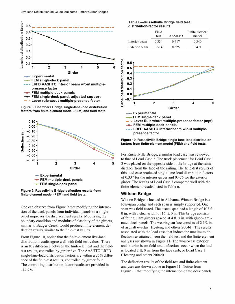
From Figure 10, notice that the finite-element live-load distribution results agree well with field-test values. There is an 8% difference between the finite-element and the field-test results, controlled by girder five. The AASHTO LRFD single-lane-load distribution factors are within a 25% differ-ence of the field-test results, controlled by girder four. The controlling distribution-factor results are provided in Table 6.

For Russellville Bridge, a similar load case was reviewed to that of Load Case 2. The truck placement for Load Case 3 was placed on the opposite side of the bridge at the same distance from the face of the railing. The field-test results of this load case produced single-lane-load distribution factors of 0.337 for the interior girder and 0.476 for the exterior girder. The results of Load Case 3 compared well with the finite-element results listed in Table 6.

Wittson BridgeWittson Bridge is located in Alabama. Wittson Bridge is a four-span bridge and each span is simply supported. One span was field tested. The tested span had a length of 102 ft, 0 in. with a clear width of 16 ft, 0 in. This bridge consists of four glulam girders spaced at 4 ft, 3 in. with glued-lami-nated deck panels. The wearing surface consists of 2 1/2 in. of asphalt overlay (Hosteng and others 2004d). The results associated with the load case that induce the maximum de-flections as attained from the field test and the finite-element analyses are shown in Figure 11. The worst-case exterior and interior beam field-test deflections occur when the load is located 2 ft, 0 in. from the face curb, or Load Case 1 (Hosteng and others 2004d).

The deflection results of the field-test and finite-element analyses are shown above in Figure 11. Notice from Figure 11 that modifying the interaction of the deck panels

–0.1

0.0

0.1

0.2

0.3

0.4

0.5

1 2 3 4 5 6Girder

Experimental

FEM multiple-deck panels


FEM single-deck panel, adjusted support

LRFD AASHTO interior beam w/out multiple-presence factor


Lane

load

dis

trib

utio

n fa

ctor

Figure 8. Chambers Bridge single-lane-load distribution factors from finite-element model (FEM) and field tests.

–0.70–0.60–0.50–0.40–0.30–0.20–0.100.000.10

1 2 3 4 5

Def

lect

ion

(in.)

Girder


Figure 9. Russellville Bridge deflection results from finite-element model (FEM) and field tests.

Table 6—Russellville Bridge field test distribution-factor results

Field test AASHTO



–0.10.00.10.20.30.40.50.6

1 2 3 4 5

Lane

-load

dis

trib

utio

n fa

ctor

Girder Experimental




Lever Rule w/out multiple-presence factor (mpf)

Figure 10. Russellville Bridge single-lane-load distribution factors from finite-element model (FEM) and field tests.

8

from individual panels to a single panel improves the dis-placement results. Finite-element analyses generated results capturing field-test values.

From Figure 12, observe the finite-element live-load dis-tribution results as they compare with the field-test values. There is a 5% difference between the finite-element and the field-test results, controlled by girder one. The AASHTO LRFD single-lane-load distribution factors are within a 13% difference of the field-test values, controlled by girder two.

The controlling distribution-factor results are provided in Table 7.

Development of Live-load Distribution Equations for Timber BridgesGeneralThe results summarized above demonstrate that the analyti-cal model produces acceptable live-load distribution factors when compared with the results of field-tested in-service bridges. However, the AASHTO load-distribution equations tended to yield results that were larger than the field-test results. Therefore, the finite-element modeling approach previously described was used to analyze a broader range of common glued-laminated timber bridges. This included 32 bridges with varying span lengths, clear widths, and gird-er spacing. The dimensions for these bridges were selected based on the Standard Plans for Timber Highway Structures (Lee and Wacker 2000). These dimensions are as follows:

• Clear width varied from 12 ft, 0 in. to 36 ft, 0 in.• Span length varied from 20 ft, 0 in. to 80 ft, 0 in.• Girder spacing varied from 3 ft, 4 in. to 6 ft, 0 in.• Overhang dimensions, from the face-of-curb to the

center of the exterior girder, varied from 12 to 30 in.

In addition, bridges with spans of 100 ft, overhang dimen-sions that varied from 0–3 ft, and various timber moduli of elasticity were also investigated. A total of 102 bridges was analyzed. Of the total bridges, 57 bridges and 45 bridges were used to determine the live distribution factors for single and multiple truck loadings, respectively.

Truck loading used in this work consisted of AASTHO’s HL-93 design loads. The AASHTO LRFD design truck (HS20) and design tandem loads were used in this study. Additionally, uniform design lane-load effects were neglect-ed. The longitudinal position of the truckload was placed to create either the maximum moment or the maximum shear in the bridge girders. The transverse position of the truck varied from 2 ft from the face of curb, moving toward the center of the bridge in one-foot increments, as shown in Fig-ure 13. A total of 10 load cases, five load cases for moment and five load cases for shear, were analyzed for each bridge. The number of load cases were reduced where limited by the clear width of the bridge. For the multiple-lane-load condition, the second truck was spaced 4 ft from the truck positions provided in Figure 13.

Live-load distribution factors were determined from the girder stress results obtained from the finite-element models. The finite-element results were compared with the current AASHTO LRFD live-load distribution factors for each bridge. Based on the results obtained from the finite-element analyses, simplified live-load distribution relations were developed for single- and multiple-design lanes. These live-load distribution relations were developed to determine the


–1.00–0.90–0.80–0.70–0.60–0.50–0.40–0.30–0.20–0.10

0.00

1 2 3 4

Defle

ctio

n (in

.)

Girder


Figure 11. Wittson Bridge deflection results from finite-element model (FEM) and field tests.

0.0

0.1

0.2

0.3

0.4

0.5

1 2 3 4Girder

Experimental



FEM single-deck panel, adjusted support



Lane

load

dis

trib

utio

n fa

ctor

Figure 12. Wittson Bridge single-lane-load distribution factors.

Table 7—Wittson Bridge field test distribution-factor results

Field test AASHTO



9


moment and shear design values for both interior and exterior girders.

Live-Load Moment-Distribution Factor for an Interior GirderFor each bridge analyzed, the current AASHTO LRFD live-load distribution factors (on the vertical axis) were plotted against the bridges’ respective finite-element results (on the horizontal axis). These plots are provided in Figures 14 and 15 for single- and multiple-lane-load conditions, respective-ly. The multiple-presence factors that are associated with the 2005 AASHTO LRFD live-load distribution factors were re-moved from the plotted results. If the live-load distribution factors obtained using the AASHTO LRFD Specification correspond similar to the finite-element results, one would expect that these results would plot a straight line with a slope of unity and would have minimal scatter.

As can be observed from the results in Figures 14 and 15, the recommended AASHTO LRFD live-load distribution factors overestimate the moment induced in an interior girder under single- and multiple-lane loadings. On average, the AASHTO LRFD single-lane-load distribution factors produced results 21% greater than the finite-element results. Similar to the single-lane-load results, the AASHTO LRFD multiple-lane-load distribution factors yielded a distribu-tion factor 7% greater than those obtained from the finite-element results.

Other published techniques used for estimating the live-load distribution factors, such as the uniform-method and the le-ver rule (Pucket and others 2006), were also evaluated. For this particular case, the uniform method was explored. The uniform-method results, obtained using Equation (3), were plotted against the finite-element results and are provided

in Figures 16 and 17 for single- and multiple-lane loadings, respectively.

(3)

Where

guniform is the uniform-method distribution factor,Ng number of girders in the bridge cross section, andWc clear roadway width (ft).

Figure 13. Design-load transverse truck placement for varying load cases (L.C.), according to ASSHTO HL-93.

y = 1.6088x – 0.1062 R² = 0.6462

0.2

0.3

0.4

0.5

0.6

0.2 0.3 0.4 0.5 0.6

2005

AA

SHTO

LR

FD d

istr

ibut

ion

fact

or(n

o m

ultip

le-p

rese

nce

fact

or)

Finite-element distribution factor

Figure 14. AASHTO LRFD, interior girder single-lane-load moment factors.

y = 1.1931x – 0.055 R² = 0.888

0.3

0.4

0.5

0.6

0.7

0.3 0.4 0.5 0.6 0.7

2005

AA

SHTO

LR

FD d

istr

ibut

ion

fact

or(n

o m

ultip

le-p

rese

nce

fact

or)


Figure 15. AASHTO LRFD, interior girder multiple-lane-load moment factors.

10

From Figures 16 and 17, notice that the uniform method would yield satisfactory results for determining the live-load distribution factor of interior girders under multiple-lane loads. On the contrary, the finite-element single-lanelane-load distribution results did not compare as well with the uniform method. This was expected because the uniform method assumes equal distribution to all girders of the bridge.

Because of the scatter of the uniform-method results shown in Figure 16, parametric relations that can be used in

determining the live-load distribution factors for glued-laminated timber bridges were developed. The parametric equation was developed using the regression analysis solver provided in Microsoft Excel (Microsoft Corporation, Red-mond, Washington). The same parametric equation can be used for single- and multiple-lane-load conditions. The equation includes variables that are known during the pre-liminary design phase. The proposed parametric equation is expressed as

(4)

where

D is the constant,exp1 constant,exp2 constant,exp3 constant,gpim parametric distribution factor of interior girder,L span length, center to center of bearing (ft),Ng number of girders in the bridge cross section,S girder spacing (ft), andWc clear roadway width (ft).

The constant “D” and the three exponents in Equation (4) were determined by the regression routine in Microsoft Excel to produce live-load distribution factors that are corre-lated to the finite-element results. The calculated values for these parameters are listed in Table 8. Equation (4) was then used in conjunction with the geometry of all of the analyzed bridges to estimate the live-load distribution factors. These results were compared with the distribution factors obtained from the finite-element analyses, as shown in Figures 18 and 19. Notice from these figures that Equation (4) produced live-load distribution-factor results that are very close to those obtained from the finite-element analyses. This can be observed from the scatter of the results of Equation (4) about the solid one-to-one line included in Figures 18 and 19. In other words, one expects the results of Equation (4) to be equal to the finite-element values; that is, with a linear relation that has a zero intercept and slope of one.

Using Excel software, the best-fit line for the ratio of the live-load distribution factors obtained using Equation (4) and the finite-element results were determined. For example, Figure 20 yields an equation for the best-fit line as y1 = 0.888x + 0.036.


y = 1.5749x – 0.051 R² = 0.5729

0.2

0.3

0.4

0.5

0.6

0.2 0.3 0.4 0.5 0.6

Uni

form

met

hod

(Eq.

(3))


Figure 16. Uniform method, interior girder single-lane-load moment factors.

y = 0.8876x + 0.055R² = 0.8827

0.3

0.4

0.5

0.6

0.7

0.3 0.4 0.5 0.6 0.7

Uni

form

met

hod

(Eq.

(3))


Figure 17. Uniform method, interior girder multiple-lane-load moment factors.

Table 8—Parametric constants for interior-beam distribution factors for moment design

Exponents

Loading D 1 2 3

Single 40 0.409 0.108 –0.018Multiple 10 0.792 0.058 –0.051

11


Notice that the ratio of Equation (4) to the finite-element results yielded a best-fit line having a slope slightly below one and an intercept slightly above zero. For Equation (4) to produce a best-fit line that has a slope of one and a zero intercept, when compared with the finite-element results, further modification was required. This modification was accomplished using the affine transformation process, as summarized by Wolfram Research (2004). The

affine-transformation process was used in NCHRP 12-62 (Pucket and others 2006). An example of the affine-transfor-mation process is as follows:

The regression best-fit equation from Figure 18 is y = 0.888x + 0.036,

which can be expressed as y = a1x + b1, where

a1 is the slope of the best-fit line,b1 intercept of the best-fit line,x the finite-element live-load distribution factor; that is, the distribution factor one would obtain using finite-element analysis, andy the distribution factor determined from Equation (4) (gpim).

The next step in the affine-transformation process is to solve for x in the equation above and substitute y for gpim:

Let

x will be referred to as gcalibrated from here.

Substituting the variables above, the final equation is as follows:

(5)

To account for any inherent variability of the results ob-tained from Equation (5), the distribution-simplification factor and the multiple-presence factor were next introduced to attain the final live-load distribution expression that will be used for design, as shown in Equation (6). The multiple-presence factor in Equation (6) is kept as a separate term for clarity.

(6)

wherea is the calibration constant, adjusts trend-line slope,b calibration constant, adjusts trend-line intercept,gpim Parametric distribution factor, interior girder (Eq. (4)) m multiple-presence factor,mg lane-load distribution factor, final adjusted factor, andγs distribution-simplification factor.

The distribution-simplification factor adjusts the mean re-sults of Equation (5) to deviate by one-half standard devia-tion. This is similar to NCHRP 12-62 (Pucket and others 2006). An example of the how the distribution-simplification factor was determined follows:

y = 0.888x + 0.036R² = 0.9055

0.2

0.3

0.4

0.5

0.2 0.3 0.4 0.5

Para

met

ric e

quat

ion

(Eq.

(4))


Figure 18. Parametric equation (Eq. (4)), interior girder single-lane-load moment factors.

y = 0.9644x + 0.0174R² = 0.9236

0.3

0.4

0.5

0.6

0.3 0.4 0.5 0.6Finite-element distribution factor

Para

met

ric e

quat

ion

(Eq.

(4))

Figure 19. Parametric equation (Eq. (4)), interior girder single-lane-load distribution factors.

12

Using the following statistical relationship in Equation (7),

(7)

where

γs is the distribution-simplification factor,μS/R the mean ratio of Equation (5) and the finite- element results, za number of standard deviations that the method is above the mean of the finite-element results, 0.5 was used, andCOVS/R coefficient of variation.

The statistical data provided from Figure 20 produces a distribution-simplification factor “γs” of

The final live-load distribution factors produced by Equa-tion (6) are shown in Figures 20 and 21 for single- and multiple-lane loads, respectively. To determine the final live-load distribution factors, the calibration constants and the distribution-simplification factor values in Table 9 were used. The multiple-presence factors were not included in the plotted results. On average, the proposed parametric equa-tion produces results 2% greater than the rigorous finite-element results because of the distribution-simplification factor adjustment.

Live-Load Shear Distribution Factor for an Interior GirderThe same bridges used above were also analyzed to inves-tigate the live-load shear distribution factors for an interior girder. The load was placed to induce the worst-case reac-tion and shear forces in the bridge girders. These finite-element results (in the vertical axis) were plotted against the current 2005 AASHTO LRFD live-load distribution results (in the horizontal axis). The single- and multiple-lane-load distribution-factor results are plotted in Figures 22 and 23, respectively. The multiple-presence factors that are associ-ated with the 2005 AASHTO LRFD live-load distribution factors were removed from the plotted results.


0.2

0.3

0.4

0.5

0.2 0.3 0.4 0.5

Fina

l liv

e lo

ad d

istr

ibut

ion

fact

or (E

q. (6

))(n

o m

ultip

le-p

rese

nce

fact

or)

R² = 0.9055y = 1.02x – 3E-05


Figure 20. Proposed alternative (Eq. (6)), interior girder single-lane-load moment factor.

y = 1.02x – 1E-05 R² = 0.9236

0.3

0.4

0.5

0.6

0.7

0.3 0.4 0.5 0.6 0.7

Fina

l liv

e-lo

ad d

istr

ibut

ion

fact

or (E

q. (6

))(n

o m

ultip

le-p

rese

nce

fact

or)


Figure 21. Proposed alternative (Eq. (6)), interior girder multiple-lane-load moment factor plotted with no multiple-presence factor (mpf).

Table 9—Interior beam live-load distribution factors for moment design

Calibration constants Factors

Loading a b ma γsb

Single 1.126 –0.041 1.2 1.02 Multiple 1.037 –0.018 1.0 1.02 a Multiple-presence. bDistribution-simplification.

γs µS/R COVS/R za Count

1.02 0.999 0.036 0.5 57


1.02 0.999 0.035 0.5 45

Calibrated Parametric Equation

13


Notice from the results in Figures 22 and 23 that the rec-ommended AASHTO LRFD live-load distribution factors underestimate the shear induced in an interior girder under single- and multiple-lane loadings. On average, the 2005 AASHTO LRFD distribution factors yielded results 3% less than the finite-element results for the single-lane-load condi-tion. Similar to the single-lane-load results, the AASHTO LRFD multiple-lane-load distribution factors yielded values 10% less than those obtained from the finite-element results.

Because of the scatter of the AASHTO LRFD live-load distribution results, parametric relations that can be used in

determining the live-load distributions for glued-laminated timber bridges were developed. The parametric equation was developed using the regression-analysis solver provided in Microsoft Excel. The same parametric equation can be used for single- and multiple-lane-load conditions. The equation includes variables that are known during the pre-liminary design phase. The proposed parametric equation is expressed as

(8)

where

c is the constant,D constant,exp1 constant,exp2 constant,gpiv parametric distribution factor of interior girder,L span length, center to center of bearing (ft), andS girder spacing (ft).

The constants in Equation (8) were determined by the re-gression routine in Microsoft Excel, as described above. The calculated values for these parameters are listed in Table 10. Equation (8) was then used in conjunction with the geom-etry of all the analyzed bridges to estimate the live-load dis-tribution factors. These results were compared with the dis-tribution factors obtained from the finite-element analyses, as shown in Figures 24 and 25. Notice from these figures that Equation (8) produced live-load distribution-factor re-sults that are near to those obtained from the finite-element analyses. This can be observed from the scatter of the results of Equation (8) about the solid one-to-one line included in Figures 24 and 25. In other words, one expects the results of Equation (4) to be equal to the finite-element values; that is, with a linear relation that has a zero intercept and slope of one.

Based on simplification and accuracy, the parametric equa-tion will be used herein to determine the distribution factor for interior girders under single- or multiple-lane loads. Similar to the approach used in NCHRP 12-62 (Pucket 2006) and as described previously, the final distribution fac-tor used for design will be determined using Equation (9). To determine the final live-load distribution factors, the cali-bration constants and the distribution-simplification factor

y = 1.0614x – 0.033 R² = 0.8533

0.2

0.3

0.4

0.5

0.6

0.2 0.3 0.4 0.5 0.6

2005

AA

SHTO

LR

FD d

istr

ibut

ion

fact

or(n

o m

ultip

le-p

rese

nce

fact

or)


Figure 22. AASHTO LRFD, interior girder single-lane-load shear factors.

y = 1.051x – 0.0776 R² = 0.8135

0.3

0.4

0.5

0.6

0.7

0.3 0.4 0.5 0.6 0.7

2005

AA

SHTO

LR

FD d

istr

ibut

ion

fact

or(n

o m

ultip

le-p

rese

nce

fact

or)


Figure 23. AASHTO LRFD, interior girder multiple-lane-load shear factors.

Table 10—Parametric constants for interior beam distribution factors for shear design Exponent

Loading C D 1 2

Single 0.92 12 0.719 0.065 Multiple 0.92 10 0.704 –0.015

14

values in Table 11 were used. The final adjusted results are plotted in Figures 26 and 27 for single- and multiple-lane loads, respectively. The multiple-presence factor is not in-cluded in these plotted results.

(9)

where

A is the calibration constant, adjusts trend-line slope,B calibration constant, adjusts trend-line slope intercept

gpiv parametric distribution factor of interior girder,m multiple-presence factor,mg lane-load distribution factor, final adjusted factor andγs distribution-simplification factor.

Live-Load Moment-Distribution Factor for an Exterior GirderThe same bridges used above were analyzed to investigate the live-load moment-distribution factors for an exterior girder. The load was placed to induce the worst-case mo-ment in the bridge girders. These finite-element results (in the vertical axis) were plotted against the current 2005 AAS-HTO LRFD live-load distribution results (in the horizontal axis). Currently, AASHTO uses the lever rule to determine the live-load moment-distribution factor for exterior girders. The single- and multiple-lane-load distribution-factor results are plotted in Figures 28 and 29, respectively. The multiple-presence factors that are associated with the 2005 AASHTO LRFD live-load distribution factors were not included in the plotted results.

As can be observed from the results in Figures 28 and 29, the recommended AASHTO LRFD live-load distribution factors overestimate the moment induced in an exterior girder under single- and multiple-lane loadings. On average, the AASHTO LRFD single-lane-load distribution factors produced results 9% greater than the finite-element results. Similar to the single-lane-load results, the AASHTO LRFD multiple-lane-load distribution factors yielded a distribution factor that is 6% greater than those obtained from the finite-element results.

Other published techniques used for estimating the live-load distribution factors, such as the uniform-method and the lever rule (Pucket 2006), were also evaluated. For this particular case, the uniform method was explored. The uniform-method results, obtained using Equation (3), were plotted against the finite-element results and are provided in Figures 30 and 31 for single- and multiple-lane loadings, respectively.

Because of the scatter of the uniform-method results shown in Figures 30 and 31, parametric relations that can be used in determining the live-load distributions for glued-laminated timber bridges were developed. The parametric


y = 0.8992x + 0.0418R² = 0.8961

0.2

0.3

0.4

0.5

0.6

0.2 0.3 0.4 0.5 0.6

Para

met

ric e

quat

ion

(Eq.

(8))


Figure 24. Parametric equation (Eq. (8)), interior girder single-lane-load shear factors.

y = 0.8485x + 0.1195R² = 0.8114

0.3

0.4

0.5

0.6

0.7

0.3 0.4 0.5 0.6 0.7

Par

amet

ric e

quat

ion

(Eq.

(8))


Figure 25. Parametric equation (Eq. (8)), interior girder single-lane-load shear factors.

Table 11—Interior beam distribution factors for shear design

Calibration constants Factors

Loading b a ma γs b

Single 1.112 1.03 –0.046 1.2 Multiple 1.179 1.03 –0.141 1.0 a Multiple-presence. b Distribution-simplification.

15


equation was developed using the regression analysis solver provided in Microsoft Excel. The same parametric equation can be used for single- and multiple-lane-load conditions. The equation includes variables that are known during the preliminary design phase. The proposed parametric equation is expressed as

(10)

µS/R COVS/R za Count

1.03 1.000 0.053 0.5 57


γ s µS/R COVS/R za Count

1.03 0.999 0.055 0.5 45


y = 1.03x + 5E-05R² = 0.8961

0.2

0.3

0.4

0.5

0.6

0.2 0.3 0.4 0.5 0.6

Fina

l liv

e-lo

ad d

istr

ibut

ion

fact

or (E

q. (9

))(n

o m

ultip

le-p

rese

nce

fact

or)


Figure 26. Proposed alternative (Eq. (9)), interior-girder single-lane-load shear factors.

y = 1.03x – 4E-05 R² = 0.8114

0.3

0.4

0.5

0.6

0.7

0.3 0.4 0.5 0.6 0.7

Fina

l liv

e-lo

ad d

istr

ibut

ion

fact

or (E

q. (9

))(n

o m

ultip

le-p

rese

nce

fact

or)


Figure 27. Proposed alternative (Eq. (9)), interior-girder multiple-lane-load shear factors.

y = 0.7822x + 0.1326R² = 0.4612

0.3

0.4

0.5

0.6

0.7

0.3 0.4 0.5 0.6 0.7

2005

AA

SHTO

LR

FD d

istr

ibut

ion

fact

orle

ver r

ule

(no

mul

tiple

-pre

senc

e fa

ctor

)


Figure 28. AASHTO LRFD, exterior-girder single-lane-load moment factors.

0.2

0.3

0.4

0.5

0.6

0.2 0.3 0.4 0.5 0.6

2005

AA

SHTO

LFR

D d

istr

ibut

ion

fact

orle

ver r

ule

(no

mul

tiple

-pre

senc

e fa

ctor

)

y = 0.6889x + 0.1355R² = 0.4065


Figure 29. AASHTO LRFD, exterior-girder multiple-lane-load moment factors.

16

where

D is the constant,de center of exterior girder to face of curb (ft),exp1 constant,exp2 constant,exp3 constant,gpem parametric distribution factor of exterior girder,L span length, center to center of bearing (ft), andS girder spacing (ft).

The constants in Equation (10) were determined by the regression routine in Microsoft Excel, as described above. The calculated values for these parameters are listed in Table 12. Equation (10) was then used in conjunction with the geometry of all of the analyzed bridges to estimate the live-load distribution factors. These results were compared with the distribution factors obtained from the finite-element analyses, as shown in Figures 30 and 31. Notice from these figures that Equation (10) produced live-load distribution-factor results that are very close to those obtained from the finite-element analyses. This can be observed from the scatter of the results of Equation (10) about the solid one-to-one line included in Figures 32 and 33. In other words, one expects the results of Equation (10) to be equal to the finite-element values; that is, with a linear relation that has a zero intercept and slope of one.

Based on simplification and accuracy, the parametric equa-tion will be used herein to determine the distribution factor for exterior girders under single- or multiple-lane loads. Similar to the approach used in NCHRP 12-62 (Pucket and others 2006) and as described previously, the final dis-tribution factor used for design will be determined using Equation (11). To determine the final live-load distribution factors, the calibration constants and the distribution-sim-plification factor values in Table 13 were used. The final ad-justed results are plotted in Figures 34 and 35 for single- and multiple-lane loads, respectively.

(11)


y = 1.168x – 0.0201 R² = 0.802

0.2

0.3

0.4

0.5

0.6

0.2 0.3 0.4 0.5 0.6

Uni

form

met

hod

(Eq.

(3))


Figure 30. Uniform method (Eq. (3)), exterior-girder single-lane-load moment factors.

0.3

0.4

0.5

0.6

0.7

0.3 0.4 0.5 0.6 0.7

Uni

form

met

hod

(Eq.

(3))


y = 0.9025x + 0.0452R² = 0.8304

Figure 31. Uniform method (Eq. (3)), exterior-girder multiple-lane-load moment factors.

y = 0.8785x + 0.0481R² = 0.9616

0.2

0.3

0.4

0.5

0.6

0.2 0.3 0.4 0.5 0.6


Para

met

ric e

quat

ion

(Eq.

(10)

)

Figure 32. Parametric equation (Eq. (10)), exterior-girder single-lane-load moment factors.

17


where

a is the calibration constant, adjusts trend-line slope,b calibration constant, adjusts trend-line slope intercept,gpem parametric distribution factor of interior girder,m multiple-presence factor,mg lane-load distribution factor, final adjusted factor, andγs distribution-simplification factor.

y = 0.9023x + 0.0467R² = 0.9294

0.3

0.4

0.5

0.6

0.7

0.3 0.4 0.5 0.6 0.7

Para

met

ric e

quat

ion

(Eq.

(10)

)


Figure 33. Parametric equation (Eq. 10)), exterior-girder multiple-lane-load moment factors.

Table 13—Exterior beam distribution factors for moment design

Calibration constants

Factors

Loading a b ma γsb

Single 1.138 –0.055 1.2 1.02 Multiple 1.108 –0.052 1.0 1.02 a Multiple-presence. b Distribution-simplification.

Table 12—Parametric constants for exterior beam distribution factors for moment design Exponent

Loading D 1 2 3

Single 12 0.643 0.075 0.127 Multiple 10 0.821 –0.008 0.166

y = 1.02x + 2E-05R² = 0.9616

0.2

0.3

0.4

0.5

0.6

0.2 0.3 0.4 0.5 0.6

Fina

l liv

e-lo

ad d

istr

ibut

ion

fact

or (E

q. (1

1))

(no

mul

tiple

-pre

senc

e fa

ctor

)

Finite element distribution factorFinite-element distribution factor

Figure 34. Proposed alternative (Eq. 11)), exterior-girder single-lane-load moment factors.


1.02 0.999 0.028 0.5 57


y = 1.02x - 3E-05R² = 0.9294

0.3

0.4

0.5

0.6

0.7

0.3 0.4 0.5 0.6 0.7

Fina

l liv

e-lo

ad d

istr

ibut

ion

fact

or (E

q. (1

1))

(no

mul

tiple

-pre

senc

e fa

ctor

)



1.02 0.999 0.034 0.5 45


Figure 35. Proposed alternative (Eq. 11)), exterior-girder multiple-lane-load shear factors.

18

Live-Load Shear Distribution Factor for an Exterior GirderThe same bridges used previously were analyzed to inves-tigate the live-load shear distribution factors for an exterior girder. The load was placed to induce the worst-case reac-tion and shear in the bridge girders. These finite-element results (in the vertical axis) were plotted against the current


0.2

0.3

0.4

0.5

0.6

0.2 0.3 0.4 0.5 0.6

2005

AA

SHTO

LR

FD d

istr

ibut

ion

fact

or

leve

r rul

e (n

o m

ultip

le-p

rese

nce

fact

or)

y = 0.8566x + 0.0574R² = 0.8955


Figure 36. AASTHO LRFD, exterior-girder single-lane-load shear factors.

y = 0.8543x + 0.0842R² = 0.8744

0.2

0.3

0.4

0.5

0.6

0.2 0.3 0.4 0.5 0.6

2005

AA

SHTO

LR

FD d

istr

ibut

ion

fact

or

leve

r rul

e (n

o m

ultip

le-p

rese

nce

fact

or)


Figure 37. AASHTO LRFD, exterior-girder multiple-lane-load shear factors.

y = 1.03x – 4E-05 R² = 0.8955

0.3

0.4

0.5

0.6

0.7

0.3 0.4 0.5 0.6 0.7

Fina

l liv

e-lo

ad d

istr

ibut

ion

fact

or (E

q. (1

2))

(no

mul

tiple

-pre

senc

e fa

ctor

)

Finite-element distribution factors

Figure 38. Proposed alternative (Eq. (12)), exterior-girder single-lane-load shear factors.

y = 1.03x – 4E-05 R² = 0.8744

0.3

0.4

0.5

0.6

0.7

0.3 0.4 0.5 0.6 0.7

Fina

l liv

e-lo

ad d

istr

ibut

ion

fact

or (E

q. (1

2))

(no

mul

tiple

-pre

senc

e fa

ctor

)

Finite-element distribution factors

Figure 39. Proposed alternative (Eq. (12)), exterior-girder multiple-lane-load shear factors.


1.03 1.000 0.055 0.5 57

Calibrated Lever Rule


1.03 0.999 0.056 0.5 45

Calibrated Lever Rule

19


2005 AASHTO LRFD live-load distribution results (in the horizontal axis). Currently, AASHTO uses the lever rule to determine the live-load shear distribution factor for exterior girders. The single- and multiple-lane-load distribution-factor results are plotted in Figures 36 and 37, respectively. The multiple-presence factors that are associated with the 2005 AASHTO LRFD live-load distribution factors were not included in the plotted results.

One can notice from the results in Figures 38 and 39 that the lever rule produced acceptable results compared with the finite-element values. On average, the 2005 AASHTO LRFD distribution factors produced results 2% greater than the finite-element results for the single-lane-load condition. The multiple-lane-load AASHTO LRFD distribution fac-tors produced values 7% less than those obtained from the finite-element results. The best-fit line equations from both plots have a slope near unity. The correlation (R2) results from both plots are large, near 0.9. Based on simplicity and accuracy, the lever rule will be used herein to determine the live-load shear-distribution factors for an exterior girder.

The lever-rule distribution factor will be adjusted using the affine-transformation process and the distribution-simpli-fication factor used in NCHRP 26-62 (Pucket and others 2006) and as described previously. The final distribution factor used for design is presented in Equation (12). The calibration constants and the distribution-simplification fac-tor are provided in Table 14. The final adjusted results are provided in Figures 38 and 39.

(12)

where

a is the calibration constant that adjusts trend-line slope,

b calibration constant that adjusts trend-line slope intercept,

glever lever-rule distribution factor of exterior girder,

m multiple-presence factor, mg lane-load distribution factor, final adjusted

factor, andγs distribution-simplification factor.

Summary of the Developed Live-Load Distribution EquationsTo replace the existing AASHTO LRFD live-load distribu-tion factors, four proposed live-load distribution equations with adjustment factors will be presented. The same equa-tion will be used for both single- and multiple-lane-load conditions. Below are the four proposed equations along with the parametric constants, as shown in Table 15, re-quired to compute the live-load distribution factors:

Interior Girder—Moment (Eq. (4))

Interior Girder—Shear (Eq. (8))

Exterior Girder—Moment (Eq. (10))

Exterior Girder—Shear

Table 14—Calibration constants for exterior beam distribution factors for shear design

Calibration constants

Factors

Loading a b ma γsb

Single 1.167 –0.067 1.2 1.03 Multiple 1.171 –0.099 1.0 1.03 a Multiple-presence. b Distribution-simplification.

Table 15—Parametric constants Constants Exponent

Girder Loading c D 1 2 3

Interior Single — 40 0.409 0.108 –0.018 Moment Multiple — 10 0.792 0.058 –0.051 Interior Single 0.92 12 0.719 0.065 — Shear Multiple 0.92 10 0.704 –0.015 — Exterior Single — 12 0.643 0.075 0.127 Moment Multiple — 10 0.821 –0.008 0.166

20

The live-distribution factors determined using the equations above are adjusted using the affine-transformation process, distribution-simplification factor, and the multiple-presence factor. The final live-load distribution factors used for design are produced by Equation (13). The calibration constants, distribution-simplification factor, and the multiple-presence factors are provided in Table 16.

(13)

where

a is the calibration constant, adjusts trend-line slope,

b calibration constant, adjusts trend-line slope intercept,

m multiple-presence factor,mg lane-load distribution factor, final adjusted

factor,γs distribution-simplification factor.

Proposed Live-Load Distribution Equation ExampleAn example of the proposed equation is provided for ad-ditional clarification. The live-load distribution factors from the field-tested Chamber Bridge will be computed and then compared with the finite-element results. Chambers Bridge represents a common glued-laminated timber bridge and is within the limits used to develop the proposed live-load dis-tribution equations. The multiple-presence factor is included in these results.

Chambers Bridge General Dimensions

de is 1.75 ftL 51.5 ftNg 6 ftS 5 ftWc 28.5 ft

Interior Girder—Moment, Single-Lane-Load Equation (4)

From Equation (13)

Interior Girder—Moment, Multiple-Lane-Load Equation (4)

From Equation (13)

Interior Girder—Shear, Single-Lane-Load Equation (8)

From Equation (13)

Interior Girder—Shear, Multiple-Lane-Load Equation (8)

From Equation (13)

The interior beam live-load distribution factors have been summarized in Table 17. The proposed equation results compare well with the finite-element results. A maximum 2% difference is observed between the finite-element results and the proposed equation results.Exterior Girder Moment, Single-Lane-Load Equation (10)

From Equation (13)

Exterior Girder—Moment, Multiple-Lane-Load Equation (10)

From Equation (13)


Table 16—Live-distribution factorsCalibration constants Factors

Girder Loading ma γsb a b

Interior Single 1.2 1.02 1.126 –0.041Moment Multiple 1.0 1.02 1.037 –0.018Interior Single 1.2 1.03 1.112 –0.046Shear Multiple 1.0 1.03 1.179 –0.141Exterior Single 1.2 1.02 1.138 –0.055Moment Multiple 1.0 1.02 1.108 –0.052Exterior Single 1.2 1.03 1.167 –0.067Shear Multiple 1.0 1.03 1.171 –0.099a Multiple-presence.b Distribution-simplification.

21


Exterior Girder—Shear, Single-Lane Load (from lever rule)

From Equation (13)

Exterior Girder—Shear, Multiple-Lane Load

(from lever rule)

From Equation (13)

The exterior beam live-load distribution factors have been summarized in Table 18. The proposed equation results compare well with the finite-element results. A maximum 7% difference is observed between the finite-element results and the proposed equation results.

Proposed Equation Comparison with the Field-Test BridgesThe four field-tested bridges were used to validate the pro-posed load distribution equations above. The single-lane-load moment-distribution factors, for interior and exterior girders, were calculated using the proposed equations and compared with the field-test results. The multiple-presence factors were not included in the results. The proposed equa-tions include the calibration constant adjustments provided by Equation (13), excluding the multiple-presence factor. The finite-element distribution factors were determined with stress results due to an HL-93 AASHTO truck load. As stated previously, the field-test distribution factors were determined with deflection results. The results for the following bridges are provided: Badger Creek Bridge, Table 19; Chambers Bridge, Table 20; Russellville Bridge, Table 21; and Wittson Bridge, Table 22.

The proposed live-load distribution equations produced results within 5% of the finite-element results for Badger, Chambers, and Russellville Bridges as expected. The pro-posed exterior-girder equation results for Badger Bridge are 9% greater than the field-test results. There is a 13% difference between the proposed factor and the field-test results of the Russellville exterior girder. The field-test re-sults for a similar Russellville load case produced live-load distribution factors of 0.337 for the interior girder and 0.476 for the exterior girder. Comparing these results with the proposed equation values, the proposed equation is with-in a 5% difference. Based on these results, one can conclude that the proposed equation results compare well with both the field-test and finite-element distribution results.

The Wittson Bridge field-test distribution factors are greater than the results from the proposed equation, as listed in Table 22. Wittson Bridge has a span length of 102 ft, which is at the limit of the span length range used in the parametric bridges used to create the proposed equations. We recom-mend that no modifications should be made to the multiple-presence factors for bridges outside of the parametric bridge range.

Table 17—Interior beam results summary

Load condition


Proposed equation

AASHTO LRFD

Moment Single 0.391 0.394 0.5— Multiple 0.469 0.474 0.5Shear Single 0.523 0.521 0.5— Multiple 0.576 0.565 0.5

Table 18—Exterior beam results summary

Load condition


Proposed equationresults

AASHTO LRFD

Moment Single 0.498 0.514 0.57— Multiple 0.479 0.493 0.475Shear Single 0.568 0.602 0.57— Multiple 0.441 0.448 0.475

Table 19—Badger Creek Bridge proposed equation results

GirderField test Proposed

Finite-element model AASHTO

Interior 0.311 0.310 0.309 0.333Exterior 0.328 0.357 0.356 0.385

Table 20—Chambers Bridge proposed equation results




Table 21—Russellville Bridge proposed equation results




Table 22—Wittson Bridge proposed equationresults




22

ConclusionsOur research evaluated the existing live-load distribution equations for glued-laminated timber girder bridges pro-vided in the 2005 AASHTO LRFD Bridge Design Speci-fication. This was accomplished by using analytical finite-element models, which were validated with field data from in-service bridges. The field data consisted of deflections and live-load distribution factors from four glued-laminated timber girder bridges. The validated finite-element models were used to perform parametric studies on a broader range of bridges to determine the controlling live-load distribution factors. From these parametric bridges, proposed distribu-tion equations were developed.

Minimal changes were made to the glued-laminated timber bridge live-load distribution equations from the AASHTO Standard Specification (1996) to the 2005 AASHTO LRFD Specification (2005). The changes that did occur to the equations consisted of the conversion from wheel to lane-load distribution factors and incorporating changes to the multiple-presence factors. The lever-rule method for exte-rior girders remained unchanged. Unlike other bridge types, glued-laminated timber girder bridges do not have separate live-load distribution factors for shear. The shear design forces are adjusted with Equation (1).

Analytical finite-element models were developed using AN-SYS (1992), a general purpose finite-element program. The finite-element model used bilinear solid “brick” elements to model the timber deck panels as well as the girders. The finite-element model allowed the user to model the as-built boundary conditions of the field-tested bridges. Using the ANSYS parametric design language greatly simplified the user input, reducing the modeling time required by the user.

The analytical finite-element models were validated with experimental field-test results. The analytical deflections and live-load distribution values were within an acceptable tolerance to the field-test results. Adjusting the deck panel interaction and boundary conditions had minimal influence on the analytical live-load distribution factors. Both the analytical and field-test results demonstrated that the controlling single-lane-load moment live-load distribu-tion factors occurred when placing the truckload 2 ft, 0 in. from the face of the curb. This was observed for both the exterior and interior girders. As the load moves toward the center of the bridge, the load distribution factor in the exte-rior and interior girders reduces.

A total of 102 bridges was analyzed with the finite-element model described above. Of the total bridges, 57 bridges were used to determine the controlling single- and 45 bridg-es to determine multiple-lane-load distribution factors. The 102 bridges consisted of bridges with longer span lengths of 100 ft, overhang dimensions of 0–3 ft, and various timber moduli of elasticity. The majority of the bridges analyzed were based on the Standard Plans for Timber Highway


Structures (Lee and Wacker 2000) and consisted of geom-etries in the following range:

• Clear width varied from 12 ft, 0 in. to 36 ft, 0 in.

• Span length varied from 20 ft, 0 in. to 80 ft, 0 in.

• Girder spacing varied from 3 ft, 4 in. to 6 ft, 0 in.

• Overhang dimensions, from the face-of-curb to the center of the exterior girder, varied from 12 to 30 in.

The analytical results from the bridges above were com-pared with the current 2005 AASHTO LRFD live-load dis-tribution factors. The AASHTO LRFD live-load distribution equations consist of the “S/D” equation and the lever rule. From these results, one can observe the need for equations with greater accuracy. Our objective was to develop equa-tions with greater accuracy, while maintaining a level of simplicity. Based on performance, the parametric equations and the lever rule were recommended. The parametric equa-tions contain constants known during the preliminary design phase. The parametric equations were developed using the regression analysis solver provided in Microsoft Excel.

To adjust for any inherent variability, the developed para-metric equations were adjusted using the affine-transfor-mation process and the distribution-simplification factor, similar to NCHRP 12-62 (Pucket and others 2006). These statistical adjustments shift the mean of the proposed equa-tion results to produce conservative values when compared with the finite-element results.

Limitations of the Proposed EquationsThe proposed equations do have limitations. These limita-tions are based on the assumptions and parameters used to create the proposed equations. The proposed equations meet the conditions already established by the AASHTO LRFD (2005) Specification and they are as follows:

• Width of the deck is constant.

• Unless otherwise specified, the number of beams is not less than four.

• Beams are parallel and have approximately the same stiffness.

• Unless otherwise specified, the roadway part of the over-hang, de, does not exceed 3.0 ft.

• Curvature in plan is less than the limit specified in article 4.6.1.2.

• Cross section is consistent with that of a glued-laminated timber girder bridge with glued-laminated timber deck panels provided by AASHTO.

For simplification, the proposed equations do not consider bridges on a skew, with a sidewalk, and the influence of dia-phragms. The equations are limited to bridges with one to two traffic lanes. The proposed live-load distribution

23


equations will produce accurate results when within the geometries listed previously.

RecommendationsBased on analytical modeling and comparison of the results above, we recommend the following:

1. The proposed distribution equations were created for glued-laminated timber girder bridges with glued-lami-nated timber deck panels only. Similar live-load distribu-tion factors should be considered for additional timber bridge types.

2. The proposed equations decrease slightly in accuracy for bridges pushing the limits of the parametric bridges. Witt-son Bridge is an example of a bridge pushing the limits of the span-length boundaries used to develop the live-load distribution equations in this report. For bridges pushing the limits of the equations, the multiple-presence factors should remain unaltered. This will aid in producing con-servative results.

3. The shear live-load distribution equations developed in this report account for the controlling shear design values. The need for Equation (1) above should be reviewed. This equation is used to investigate shear parallel to the grain of the glulam girders and increases the distributed shear load determined with the existing AASHTO LRFD live-load distribution factors.

4. Further comparisons of the developed live-load distribu-tion equations with additional field-test data is recom-mended for further validation of the equations.

ReferencesAASHTO. 1996. Standard specifications for highway bridg-es. 16th ed. Washington, DC: American Association of State Highway and Transportation Officials.

AASHTO LRFD. 2005. LRFD bridge design specifications. Washington, DC: American Association of State Highway and Transportation Officials.

ANSYS. 1992. User’s manual for revision 5.0, Procedures. Canonsburg, PA: Swanson Analysis Systems, Inc.

Cai, C.S. 2005. Discussion on AASHTO LRFD load distri-bution factors for slab-on-girder bridges. Practice periodi-cal on structural design and construction, 10(3): August 1. American Society of Civil Engineers.

Cha, H. 2004. Analysis of glued-laminated timber girder bridges. Ames, IA: Iowa State University. M.S. thesis

Forest Products Laboratory. 1999. Wood handbook—Wood as an engineering material. Gen. Tech. Rep. FPL–GTR–113. Madison, WI: U.S. Department of Agriculture, Forest Ser-vice, Forest Products Laboratory. 463 p.

Gilham, P.C.; Ritter, M. 1994. Load distribution in longi-tudinal stringer-transverse deck timber bridges. Madison,

WI: U.S. Department of Agriculture, Forest Service, Forest Products Laboratory.

Hosteng, T.K. 2004. Live load deflection criteria for glued laminated structures. Ames, IA: Iowa State University. M.S. thesis.

Kurian, A.V. 2001. Finite element analysis of longitudinal glued-laminated timber deck and glued-laminated timber girder bridges. Ames, IA: Iowa State University. M.S. thesis.

Lee, P.H.L.; Wacker, J.P. 1996. Standard plans for timber highway structures. national conference on wood trans-portation structures. In: Ritter, Michael A.; Duwadi, Sheila Rimal; Lee, Paula D. Hilbrich, eds. 1996. National confer-ence on wood transportation structures. Gen. Tech. Rep. FPL–GTR–94. Madison, Wl: U.S. Department of Agricul-ture, Forest Service, Forest Products Laboratory. 494 p.

Pucket, J.A., Mertz, d., Huo, X. S., Jablin, M. C., Peavy, M. D., Patrick, M. D. 2006. Simplified live load distribution factor equations. NCHRP Report for 12-62. Transportation Research Board, of the National Academies, Washington, D.C.

Hosteng, T., Phares, B., Wipf, T., Ritter, M., Wood, D. . 2004a. Live load deflection of timber bridges, 1. Badger Creek glued-laminated girder bridge. Ames, IA: Iowa State University, Bridge Engineering Center.

Hosteng, T., Phares, B., Wipf, T., Ritter, M., Wood, D.2004b. Live load deflection of timber bridges, 7. Cham-bers County glued-laminated girder bridge. Ames, IA: Iowa State University, Bridge Engineering Center.

Hosteng, T., Phares, B., Wipf, T., Ritter, m., wood, d. 2004c. live load deflection of timber bridges, 6. Russellville glued-laminated girder bridge. Ames, IA: Iowa State University, Bridge Engineering Center.

Hosteng, T., Phares, B., Wipf, T., Ritter, M., Wood, D. 2004d. Live load deflection of timber bridges, 5. Wittson glued-laminated girder bridge. Ames, IA: Iowa State Uni-versity, Bridge Engineering Center.

Yousif, Z.; Hindi, R. 2005. Discussion on AASHTO LRFD load distribution factors for slab-on-girder bridges. Journal of Bridge Engineering. 12(6) November 1. American Soci-ety of Civil Engineers.

Weisstein, Eric W. “Affine Transformation.” From Math-World–A Wolfram Web Resource. http://mathworld.wol-fram.com/AffineTransformation.html

Zokaie, T., Mish, K. D., and Imbsen, R. A. (1995). Distribu-tion of wheel loads on highway bridges, phase 3. NCHRP 12-26/2 Final Rep., National Cooperative Highway Re-search Program, Washington, D.C.

live-load distribution on glued-laminated timber girder bridges

Documents