load scheduling with cogeneration and real time …
TRANSCRIPT

LOAD SCHEDULING WITH
COGENERATION AND REAL TIME
PRICING
By
Dawid J Erasmus
Submitted in partial fulfilment of the requirements for the
degree
Master of Engineering (Electrical)
In the
Faculty of Engineering
UNIVERSITY OF PRETORIA
©© UUnniivveerrssiittyy ooff PPrreettoorriiaa

A special word of thanks to Mike Rossouw, General Manager Engineering for theallowing me to conduct postgraduate studies. Also thank you to RBM Managementfor the financial support.

The increase in energy costs, restructuring of electricity supply industry, quality of
supply standards and environmental responsibility, initiated an investigation to utilize
available carbon monoxide for cogeneration at an industrial site. A literature study
indicated that most of the elements involved in establishing a cogeneration plant, were
investigated individually, but had not been evaluated as a system with an indication of
their relationships.
The main objective of this study was to create a methodology to evaluate the impact
of load scheduling, cogeneration and electrical tariff structures on the energy cost of
an industrial operation. A modelling methodology was developed to evaluate the
requirements for each of the elements, which were identified as the following
processes:
Plant and stockpiles
Gas and fuel
Power generation technology
Electricity tariffs
Financial evaluation
Each of the processes' input requirements were evaluated in terms of being sufficient
in providing either useful information or a model from which information could be
manipulated.
This methodology was then applied to a titanium slag producer with electric arc
furnaces and excess carbon monoxide, which was burnt and treated as waste.

Die verhoging van energie pryse, herstruktuering van
elektrisiteitsvoorsieningsindustrie, standaarde vir elektrisiteitsvoorsiening en
omgewingsbeheer het aanleiding gegee tot die ondersoek van die gebruik van
beskikbare energie bronne vir kogenerasie by 'n industriele aanleg. 'n Literatuur
studie het aangetoon dat die elemente betrokke by die daarstelling van 'n sodanige
kogenerasie aanleg, individueel ondersoek was, maar nie as 'n eenheid of 'n sisteem,
waarvan die onderlinge atbanklikheid ondersoek was nie.
Die hoofdoelwit van hierdie studie is gerig daarop om 'n metodiek te ontwikkel
waarmee die invloed van lasskedulering, kogenerasie en elektrisiteitstariewe
ondersoek kan word op die energie kostes van 'n industriele aanleg. 'n Model
metodiek is ontwikkel om die vereistes van die elemente, wat as prosesse
geidentifiseer is, te ondersoek:
Aanleg en storing
Gas en brandstof
Elektrisiteitsopwekkings tegnologie
Elektrisiteitstariewe
Finansiele ontleding
Elk van die prosesse se insetvereistes word ondersoek en uitspraak word gelewer oor
die voorsiening van, of inligting, of 'n model, waarmee inligting verkry kan word.
Hierdie model word dan toegepas op 'n titanium dioksied produseerder met elektriese
boogoonde en afval koolstof monoksied, wat verbrand word.

AC Access Charge
AL Additional Load
BC Basic Charge
BFG Blast Furnace Gas
CBL Customer Baseline Load
CCG Combined Cycle Generation
ClIP Combined Heat and power generation Plant
CO Carbon Monoxide
COG Coke Oven Gas
DSM Demand Side Management
EDF Electricite de France
ESI Electricity Supply Industry
IPC Integrated Pollution Control
IPP Independent Power Producer
IRR Internal Rate of Return
LCC Life Cycle Costing
LD Linz Donawitz
LDG LD Furnace Gas
LHV Low Heating Values
LNG Liquified Natural Gas
MR Monthly Rental
MRG Methane Rich Gas
MWe Mega Watt Electric
NER National Electricity Regulator
NPV Net Present Value
NP New Profile
PGP Power Generating Plant
RL Reduced Load
RTP Real Time Pricing

RTP}
RTP2
lIMe
MSP
DE&S
RBM
NP
Real time price including the profit adder.
Real time price excluding the profit adder
heavy mineral concentrate
Mineral separation plant
Duke Engineering and Services Mrica, Inc.
Richards Bay Minerals
New Profile

Title Page
Acknowledgement
Thesis Summary
Opsomming van Verhandeling in Afrikaans
List of Abbreviations
Table of Contents
Chapters
Reference List
Appendices A - E
(i)
(ii)
(iii)
(iv) - (v)
(vi) - (x)
1 -74
75 - 76
AI-El
1.2.1 Environmental aspects
1.2.2 Quality of Supply
1.3 Problem identification
1.4 Main objective
1.5 Specific objectives
1.6 Conclusions
1.0 PROBLEM IDENTIFICATION AND BACKGROUND 1
1.1 Introduction 1
1.2 Government policy options and electricity regulatory issues 1
3
5
6
8
8
9
CHAPTER 2
2.0 MODELLING METHODOLOGY
2.1 Introduction
Table of Contents
Page
2.2 System requirements and evaluation 11
2.2.1 Plant operations and stockpiles 13
2.2.2 Evaluation of gas or fuel 13
2.2.3 Evaluation of power plant technologies 14
2.2.4 Evaluation of electrical tariff structures 15
2.2.5 Evaluation of financial aspects 15
2.3 Cogeneration as a system 16
2.4 Conclusion 16
CHAPTER 3 18
3.0 GAS OR FUEL 18
3.1 Introduction 18
3.2 Gas composition and energy content 18
3.3 Gas quantities 20
3.3.1 Flow measurements 20
3.3.2 Useful information to collect 21
3.3.3 Verification of theoretical values 22
3.4 Verification of building block for gas or fuel 23
3.5 Conclusion 24
CHAPTER 4
4.0 POWER GENERATION PLANT
4.1 Introduction
4.2 Power generating technology
4.2.1 Preliminary evaluation

4.2.2 Cogeneration with gas turbines
4.2.3 Gas turbine fuels
4.3 Power generation plant
4.4 Verification of building block for power plant
4.5 Conclusion
Page
27
28
30
32
33
CHAPTERS
ELECTRICAL TARIFFS
5.1 Introduction 34
5.2 Scope and objectives of real time pricing tariff 34
5.2.1 CBL calculation 36
5.2.2 RTP bill calculation 37
5.2.3 Night save tariff overview 38
5.3 Model for RTP tariff evaluation 39
5.4 Verification of building block for tariff structures 41
5.5 Conclusion 41
CHAPTER 6 42
6.0 FINANCIAL EVALUATION 42
6.1 Introduction 42
6.2 Profitability of a cogeneration plant 42
6.3 Commercial availability model for cogeneration feasibility 44
6.4 Tariff evaluations with cogeneration 46
6.5 Verification of building block 46
CHAPTER 7
7.0 CASE STUDY 49
7.1 Introduction 49
7.2 Overview of typical operation of mineral sands operation 49
7.3 Plant operations and stockpiles 50
7.3.1 Verification of building block for plant operations (case 53study)
7.4 Evaluation of gas or fuel 547.4.1 Verification of building block for gas or fuel evaluation (case 55
study)
7.5 Power generation technology 56
7.5.1 Gas boiler and steam turbine configuration 57
7.5.2 Combined cycle generation (CCG) 58
7.5.3 Verification of building block for power plant technology 58evaluation (case study)
7.6 Tariff evaluation 59
7.6.1 Verification of electrical tariff evaluation building block 61
7.7 Financial evaluation 62
7.7.1 DE&S model 62
7.7.2 Tariff evaluations (case study) 64
7.7.3 Tariff evaluation (case 1) 657.7.4 Tariff evaluation (case 2) 66
7.8 Verification of financial aspects building block 68
7.9 Verification of building blocks as a system. 68

Page
CHAPTER 8 70
8.0 CONCLUSION AND RECOMMENDATIONS 70
8.1 Introduction 70
8.2 Conclusion on main objective 70
8.3 Conclusion on specific objectives 71
8.3.1 Conclusion on the development of a modelling methodology 71
8.3.2 Conclusion on plant operations and stockpiles evaluationmethodology 72
8.3.3 Conclusion on gas or fuel evaluation methodology 72
8.3.4 Conclusion on power plant evaluation methodology 72
8.3.5 Conclusion on electricity tariff evaluation methodology 73
8.3.6 Conclusion on financial evaluation methodology 73
8.4 Recommendations 74

The objective of this chapter is to provide background information on aspects that
motivated this study. Problem identification will then be motivated with information
obtained from a literature search, which was studied during the research.
Energy efficiency awareness, environmental awareness and turmoil in the electricity
supply industry were the driving forces to initiate this study on cogeneration options with
real time pricing tariff optimisation, through which possible electricity cost increases can
be countered. Conclusions of a global survey conducted [1], shows that the established
electric utilities began to discover that power production by smaller cogenerators could be
economically justified when compared with their own long term avoided cost of
production of such increments of load. The philosophy has since spread to other countries,
and "non-utility" generation is being promoted with the expectation and achievement to
reduce electricity cost. The importance of cogeneration is confirmed in countries such as
Colombia [2], Japan [3], Taiwan [4] and Canada [5]. The potential for cogeneration in
South Africa has been investigated in 1993 and shows that a total of 1471 MW was
possible [6], which can be broken down as 1290 MW for chemical and fuel processing, 60
MW for sugar and 121 MW for metal manufacturing.
The National Electricity Regulator (NER) as the controlling authority of the Electricity
Supply Industry (ESI) in South Africa has the specific objective "to exercise control over

the electricity supply industry so as to ensure order in the generation and efficient supply
of electricity." Thus the NER, established under the Electricity Act, has powers to regulate
private generation whether for use internally in the industry concerned, or in the event of
sale to the next consumer and in that case to monitor the charges. With the NER being a
government controlled regulatory body, it provides the government with the opportunity to
make certain policy decisions, which will be quantified next.
Firstly, the state of the country's economy is an important factor which will guide
government to make policy decisions that may result in reinvestment in industry and
renewed trading which in turn will impose a demand on electricity generating capacity. A
capability of obtaining power plants in as short a time as possible would become a
necessity and this could be accomplished by adopting a policy of encouraging small
private generation or cogeneration. This cogeneration should be of sufficient capacity for
own requirements with excess for resale to adjacent communities, which will be promoting
the Independent Power Producer (IPP) concept. The IPP's are broadly classified as those
sectors of industry where cogeneration was both technical and economically feasible for
generating electricity for own use or for exporting or selling to other consumers.
The second reason for such a policy would be the result of government priorities to utilise
capital funds for building programs of domestic housing and electrification, educational
expansion projects and other social upliftment activities. The funding of these may
compete with that for the construction of new power stations. If power station funding in
particular and perhaps some of the other programs could be undertaken by the private
sector, the funding by government would be considerably less.
The utility in South Africa, Eskom, is at present a juristic body established in terms of the
Eskom Act (no 40 of 1987). It has no shareholders and is seen by many as a national asset.
The Eskom Act also provides that Eskom does not pay income tax. With the promulgation
of the new Eskom Amendment Bill that was approved by Parliament on 11 June 1998, the

Minister of Public Enterprises will take the necessary steps to make Eskom a company,
with the State as the sole shareholder [7]. The privatisation of the ESI has been and still is
a contentious issue and there could be pressure to retain statutory control of Eskom, for
example simply on the grounds that the supply of power could be controlled, and cross-
subsidisation to finance less profitable rural electrification, more easily applied. Electricity
may also be more readily taxed in order to augment government monetary resources. Even
if the ESI is privati sed, the money required to subsidise rural electrification can be
obtained from normal taxation sources, which are more widely spread over the economy,
and private electricity generation can be taxed anyway. The advantage to government
however is that the capital amounts required for the expansion of power generation must
also be privately secured and that competition between generators and distributors of
electricity should assist to keep the price of electricity to an optimum low.
At this stage the Electricity Supply Industry (ESI) is in the process of major change
without clear indication on the expected outcome and this leads to uncertainty about the
future electricity prices.
Information from the EDF (Electricite de France) in [8] clearly shows that coal is used to
produce 40% of the world's electricity and the planet has sufficient reserves for the next
250 years [8]. Coal consumption is set to double between now and 2015 and this growth in
consumption of coal for electricity generation will be subject to stringent international
regulations to ensure environmental protection. On the question of the preservation of the
environment, effective contributions to the reduction of pollutants such as S02 occurring in
both the combustion of coal, or in ash, or from the effiuent run-off from the dumps of
discarded coal, would have widespread support, not only from those living in the coal
producing areas, but also in adjacent territories which might be affected by acid rain.
Providing incentives to install de-sulphurisation plants at coal or oil-fired power stations,

should be an effective means to promote control of this aspect, and direct subsidies or tax
deductions in respect of the capital expenditure for the plant should be considered.
Creating a more environmentally sustainable future is one of the greatest issues facing us
and there is a need for a national database, to be utilised for the storage and access of air
quality data which has been collected throughout the country [9].
More importantly, the assurance of adequate quality control of data being generated by
monitoring activities throughout the country is required. This will result in central planning
and effective utilisation of resources and funds to support Integrated Pollution Control
(IPC) objectives. If this is implemented it will put a lot of pressure on any organisation or
company whose emission levels are not within regulatory standards.
These pressures as well as the incentives would encourage the use of fluidised-bed
combustors for burning discarded coal or bunker fuel oil, thus achieving a desirable
objective also of utilising this waste material and conserving more high grade energy
resources. Likewise the use of hydraulic power plants will reduce the production of C02
into the atmosphere from equivalent coal burning plants.
The above aspects may also be interpreted that there is a need for environmental regulatory
bodies to set more stringent objectives and that must be seen as a warning to others who do
pollute the atmosphere with less aggressive emission levels, such as flaring and burning of
furnace off-gas

Worldwide, the financial cost implications of poor quality of electricity is being measured,
quantified and analysed. Poor power quality impacts are always translatable, albeit with
difficulty, into economic or financial terms. With the implementation of NRS048 as an
industry standard in May 1997, the NER has decided that the initial compliance would be
enforced with discretion but it would be necessary to concentrate on data collection [10].
This would assist with the establishment and refinement of the benchmarks set for the
various quality supply parameters. The NRS048 specifies the compatibility level and
assessment methods for quality parameters such as voltage and frequency regulation
requirements, voltage pollution limits for harmonic distortion, flicker and voltage
unbalance as well as specifications for supply interruptions and voltage dips.
By addressing only one aspect of quality of supply, Erasmus [11] has demonstrated that
with the implementation of NRS048, the electricity supply network has not changed but
new rules were implemented. He further demonstrated that, for the industry, electricity is
an important operating requirement, which contributes to the economic growth of the
country and that careful consideration should be given to the business case before NRS048
is implemented as a universal standard. Mitigation technologies and equipment exists but
can be capital intensive without reaching unrealistic targets.
A utility generator normally generates perfect voltage waveforms with high supply
reliability. Quality is adversely affected in the transmission and distribution process,
which will result in consumers suffering loss of production, and equipment such as
semiconductor fuses in variable speed drives, due to commutation failure caused by dips.
In South Africa, most of the power-generating stations are centralised inland where the
coal resources are, with very large consumers at remote distances from the source. The
transmission lines stretch over vast distances and different terrain forms, which also have
an impact on the quality of supply. One possible solution would be to provide some
generating capacity closer to the load to neutralise these effects. The typical utility coal

fired power station would be uneconomical due to the unavailability of the coal, which will
have to be transported to site.
This then places the focus on the option discussed earlier, namely, the power production by
smaller cogenerators or independent power producers such as chemical and fuel processing
industry, sugar industry, wood, paper and pulp industry and metal manufacturing industry.
This study was also partly motivated base on specific requirements for investigating
cogeneration for a industrial plant that produces titanium dioxide, with Carbon monoxide
gas which is treated as waste. The threats of increase in cost of energy, uncertainties in the
ESI with quality of supply issues were the main motivational factors for this study.
In view of the need to further investigate the cogeneration option for the metal industry in
South Africa, it will be necessary to provide some information to demonstrate the
unavailability of certain information. Anderson [6] has indicated that the total potential
from cogeneration is nearly 1500 MW and is shown in Table 1.1

This survey was published in 1993, with a subsequent change in the metal manufacturing
in 1995. This was the installation of a 50 MW cogeneration plant at Samancor's Meyerton
Works in Vanderbijlpark [12]. In a search for additional information on how this project
was approached, it was found that very little information was published.
A survey on the non utility generators [6], in the United States of America, has revealed
that cogeneration is more readily applied in certain industries which contribute about 70%
of the total 32 880 MW between five major industry groups as illustrated in Table 1.2.
Installed ca acit22,821,721,310,08,17,03,32,71,41,7
In the United Kingdom and Western Europe cogeneration is better known in the form of
combined heat and power where most of this generation is utilising natural gas and does
have an 11,2 % contribution from iron and steel industries. If one considers the information
available on cogeneration for metal mining and manufacturing, it is clear that it is not as
prominent as for instance the chemical and fuel, forestry and wood and coal industry.
Also, an additional factor, is the secrecy amongst and within the titanium oxide or slag
producing companies within the metal industry market, who mainly process mineral sands,
for which limited information is published regarding their operations and processes. This is
confirmed by the literature search and first hand experience that they deemed that type of
information as propriety which can have a negative influence on their position in the
competitive market. From this evaluation and the need to investigate a cogeneration plant

on a titanium oxide producer, the opportunity was identified to provide building blocks on
the methodology that should be followed when evaluating a cogeneration option for such
an industry. The relationship and dependency of the various building blocks can then be
evaluated as a system.
The main objective of this study is to create a methodology to evaluate the impact of load
scheduling, cogeneration and real time pricing on the energy cost of a typical titanium
mineral producer in the mineral sand industries.
To be able to satisfy the main objective, the following specific objectives can be used as
goals:
1.5.1 Develop a modelling methodology for a cogeneration feasibility study with the aid
of building blocks and determine the relationship of the processes identified, as a
system.

From information obtained from literature and practical experience, the following can be
concluded:
• Companies in the chemical, sugar, wood and pulp industrial sectors do make use of
available resources for cogeneration.
• Most information available was conducted on operations that have steam available for
cogeneration as well as on those with a combination of steam and natural gas. The iron
and steel industry does make use of water for roof and wall cooling which is the start of
the steam process, whilst electric arc furnaces have only recently adopted this method
on a small scale.
• A clear distinction is made in the metal and steel industries between operations with
electric furnaces which make use of blast furnaces, coke ovens, the Linz Donawitz
(LD) process and electric arc furnaces. Process related information is more readily
available on the first three types with more secrecy regarding the electric arc furnace.
• A world-wide investigation of competitors in the mineral sands industry, who provides
titanium minerals, has revealed that none of them make use of the gas from their
electric arc furnaces for cogeneration.
• Research which has been published, focuses on the individual components such as
power plants and real time pricing optimisation techniques, without taking into

consideration the need for evaluating the combination thereof No general methodology
exists that will provide building blocks to evaluate the complete system.
• Investigation on power generation equipment has proved that the technology exists and
has been implemented in cogeneration plants world-wide.
• Implementation of cogenerators has proved to be of a supportive nature for integral
planning on electricity load planning in various countries.
• It is clear that there are various activities within the South African electricity supply
industries that warrants an investigation into the utilisation of all possible energy
resources for generation of electricity.

Energy efficiency is likely to be one of the performance measurement areas in most energy
intensive operations due to the percentage contribution in operational cost. Cogeneration is
only one of the aspects that can make a contribution towards improving energy efficiencies
by making use of available energy resources that are treated as waste.
The purpose of this chapter is to represent a methodology that will provide a general
problem solving methodology for handling the decision making process for the
implementation of cogeneration with the components thereof The objectives set in Chapter
1 to provide building blocks will be developed and evaluated individually. The relationship
and the need to obtain information from the other building blocks will determine the
structure of the building blocks as a system. The functional flow diagram will then be used
to evaluate the implementation of cogeneration with real time pricing as a case study.
Evaluation refers to the examination and judgement of a system or an element of the
system in terms of worth, quality, and degree of effectiveness. The purpose is to determine,
through a combination of prediction, analysis and measurement, the true characteristics of
the system and to ensure that it successfully fulfils its intended mission. For this study it
will not be an interactive process, which will be repeated to obtain the best outcome, but
merely a framework that can be used to improve in further studies.
The building block concept that will be used is illustrated in Figure 2.1 [13] [14] [15], and
consists of only three components namely:

Process. That consists of operational activities that may have an influence on the
process.
Output. The outputs which are generated as a result of the operational activity
within the process.
Each of the processes will now be constructed on the building block principle with the
identification of inputs and outputs.

In terms of the objectives set for establishing a cogeneration plant, one must determine the
availability of energy resources that can be used for cogeneration within the plant
operation. This process, with energy input and output parameters is illustrated in Figure
2.2. This process to determine the energy sources is site specific and will only be discussed
and illustrated in the case study.
1
Plant operations &
stockpiles
This process is the methodology used to obtain sufficient information on the energy
components of the gas or fuel available, to be able to make a decision to proceed to the
next step. The building block shown in Figure 2.3, shows that the input requirements
consist mainly of measurements, sampling and analyses, which is data accumulation. That
will provide information on the quantities, composition and energy content, which are the
output parameters which will influence the next step of the system.

MeasurementAnalysis
Sampling
Output
Quantity
Composition
Energy content
Evaluation of gas
or fuel
This is also to provide a methodology on how to obtain sufficient information on the
availability of expertise and power plant technology. The dependency of this building
block on the others will be demonstrated. From building block in Figure 2.4, information
seems to be the primary requirement for the power plant selection, which can provide
information to decide the concept of the technology application depending on energy type
and quantities.
Literature searchOther applications
Evaluation of
power plant
technologies
Application model
out

This process will give a methodology on how to obtain tariff structure information and to
show how it can influence your decision-making process. Again the input requirements as
shown in Figure 2.5, to influence the evaluation process will be information and a good
understanding of the tariffs available.
Literature searchOther applications
Evaluation of
Electrical tariff
The financial evaluation process will show the methodology and models required to
evaluate this aspect and to assist with the decision making process. The outcome of this
process should give a clear indication on whether the cogeneration plant is feasible or not.
Output
Capital cost
Generation costCogeneration
Capacity
Commodity prices
Evaluation of
financial

The various components or elements as identified in this study will each be individually
evaluated in terms of the building block methodology, with an evaluation of the outcome
(outputs), to assist with the decision-making for the next step. The building blocks
discussed in paragraph 2.2.1 to 2.2.5 have been identified by means of a number inside the
block to identify the specific process. These processes can be evaluated in series or in
parallel groups. This process dependency will ensure that sufficient information is
available at the correct phase, to improve on the decision-making process on the success or
failure of the cogeneration study. The relationship and the outcomes of each of the
individual building blocks and is illustrated in Figure 2.7, where the question is represented
by means of the trapezium shape with the question mark.
From the output of each block, information and data obtained should be evaluated to
enable one to make a decision on the next step. The question to be raised is simple in that
one should evaluate the need to proceed to the next building block or not. There can only
be two outcomes, namely yes or no. The approach in obtaining solutions for the five
building blocks can be done individually or in groups, which will speed up the process, and
that relationship will be investigated as part of this study.
The evolution of a design is illustrated by [14], and amplified in a process or system as
shown in Figure 2.7. There are checks and balances in the form of reviews at each stage of
the design progression and a feedback loop for corrective action. This preliminary design
process in this chapter would assist in setting a framework that can be improved through an
iterative approach for this cogeneration study.

<:> N3
Technology
y
1 <:;>Plant N4
Tariff
N
N5
Financial

The methodology as described in the previous chapter will now be confirmed, the input
and output requirements will be evaluated and it will be verified whether it will be
sufficient to make decisions.
One of the specific objectives was to identify how much gas will be available. The energy
content of the gas is the more specific requirement as that will determine the electrical
generating capacity of the CO gas. This is in fact very simple and can only be achieved
through theoretical calculations or on-site measurements. It is always useful to verify
theoretical or design values with actual measurement.
As identified by [6], the chemical and fuel processing industry is perhaps the major
potential contributor to power generation in view of its requirements for both electric and
steam for processing. A specific example is Sasol, which generates about half of its
electrical power needs. The sugar industry uses its residue material as fuel, which is
seasonal and available during cropping. In the wood, the paper and pulp industry obtain the
raw material from the forests, which can be used as fuel but need to be supplemented with
coal in most cases. The metal manufacturing industry has the potential for producing
electrical power from various sources of gaseous material, which become available during
the manufacturing of metal concentrates, pure metals or alloys. These sources of gas are
from the manufacture of coke from coal or from the various types of furnaces.

The various metallurgical processes used for the different iron and metals will influence
the gas composition. For instance the oxygen and fuel burners can be added as
supplemental power sources with the primary aim to increase productivity.
Information on electric furnaces [16] has indicated that iron and steel industries' gases
produced by the process have Low Heating Values (LHV) in the region of 800 kCalINm3
(3300 kJlNm3) for Blast furnace gas. Although these figures are quoted without giving any
additional information, it is worth noting the availability of additional energy resources.
One important aspect about the composition of recovery gases is that they have high
impurity levels and must therefore be treated. This will have an impact on the power plant
configuration and one will have to investigate the availability of natural gas as an
additional energy source if required.
As an example to illustrate the typical composition of recovery gases, the BFG, COG,
LOG with the exception of Electric arc furnace gas, which is not available due to secrecy
aspects, is shown in Table 3.1
The gas composition can be obtained by taking various samples at different positions
within the plant to be analysed by a reputable laboratory. The importance of detailed gas
analyses is further supported by the fact that the detailed content of the gas needs to be
known in order to determine to which extent the gas cleaning needs to be done.

Component BFG COG LDG% volume dry % volume dry % volume dry
H2 2,5 60,3 1,0CO 22,8 5,0 69,2N2 53,5 4,5 14,9CH. - 25,3 -CO2 21,2 1,3 14,6CnIDn - 3,6 0,3LHV (kCaVNmJ
) 780 ± 60 4500 ± 290 2030 ± 150
Inspection of the design specifications and drawings is usually a good starting point for any
plant, if available. This will provide some information on the use of the carbon monoxide
as part of the process by other parts of the plant. It will also show the minimum and
maximum values. The level of accuracy required would depend on whether the
requirements will only be for evaluation or design purposes.
The following technologies or measurement methodologies are available for gas
measurement in a pipeline and should be carefully selected for the specific application
[17]:
Micromanometer (Pilot tube based system)
Thermal mass flowmeter
Annubar flowmeter
Hot-wire anemometer

Experience in the field of measurement has indicated that the hot-wire anemometer and the
ultrasonic type sensor are not the most reliable in this type of application and therefore
only specifications for the others are shown as per Table 3.2.
Temperature°C
-5 to 50
Accuracy%1
OtherfacilitRS232
0,07 to 46 -18 to 60 2 4 - 20 mAmass
flowmeterT 91
Annubar o to 70 >200 1 4-20mAflowmeter
The major disadvantage of the micro manometer is that it has to be installed very precisely
into the flow area in order to prevent erroneous measurements and is relatively cheap,
which is an advantage. Thermal mass flowmeters have the facility to be coupled to a
datalogger and are relatively expensive.
Annubar flowmeters need to be connected to a highly sensitive differential pressure
transducer and are in the same price range as the thermal mass flowmeter. Although the
micrometer is relatively cheaper, the installation requirements may be a disadvantage.
The CO gas flow rate based on furnace power can be expressed for various production
conditions such as normal, average, peak and design values. There will seldom be a

minimum value as most production furnaces are capital intensive and will be operated at
most economic productive levels.
Relationships between CO gas production and furnace load to be obtained from where the
minimum and maximum consumption rates as part of process should be conducted to
determine the quantities being flared.
For more accurate evaluation it may be necessary to verify the known theoretical
quantities with the measurements taken by means of the field instrumentation and gas
analyses.
The reason for this is to determine if there is a relationship between the furnace production
and the other sections of the plant. If the whole process is not constant and provision is
made for stockpiles, then the process flow will not be constant. The primary and secondary
plant operations may therefore be flexible and vary their production output, which means a
variation in CO gas consumption.
Actual measurements over a minimum of a two-week time period is recommended to
obtain a reasonable level of confidence. Any deviations from normal production profiles
should be investigated to determine the need for additional measurement.
It will also be advantageous to do the field measurements of the gas quantities, over the
same period as the power and gas evaluations.

Information obtained from this practical approach should now be evaluated to determine
whether it is sufficient to make any decisions and determine an outcome for the next step.
Refer to Figure 3.1 for the discussion that follows.
The basic information, which will determine whether it will be viable to consider a
cogeneration plant for any specific application is simply the quantity of CO gas available
with energy content. It is not critical to obtain gas cleanliness information, as this can be
recycled as part of an interactive process for further evaluation.
Input
MeasurementAnalysis
Sampling
Output
Quantity
Composition
Energy content
Let's summarise the input and output requirements for this building block from the
information gathered in the previous discussions:
Measurement of power levels and CO gas volumes.
Take sufficient CO gas samples for composite laboratory analysis.
Analyse the consistency of CO gas availability.

Energy content of CO gas to calculate the electrical capacity.
Composition of CO gas obtained from samples taken to assist with defining the
cleaning requirements.
The availability and variability of the CO gas will have an impact on the power plant
selection and if they were very stochastic by nature, an additional makeup fuel would be
required.
The volumes of gas consumed by the operations are very constant with clearly defined step
changes such as when parts of it are switched on or off The evaluation to release all CO
gas for electricity generation, and convert all the plant internal CO gas consumers to
natural gas should be conducted. In some cases, where the infrastructure exists and the
price of natural gas is relatively low, it may be feasible, otherwise it can be very expensive.
In furnace intensive operations the relationship between CO gas volumes produced is
proportional to the plant electricity consumption. However, due to the erratic nature of the
furnaces, stable gas consumption by the various plants, the excess CO availability is erratic
with very high rates of change, which can be a constraint on any power generator turbine.

Cogeneration installations worldwide may have in common the use of similar hardware,
but most installations are unique for being optimised for its own specific plant or industry
application. The type of power generation is dependent on the type of fuel available and
this chapter will provide additional background information to confirm that there is in fact
sufficient technology and expertise available for any specific application. The information
obtained from the previous chapter should now be sufficient to develop the input and
output requirements of the next building block and to determine its relationship to the other
building blocks for further decision-making.
In observing the power generating capacity of only the South Africa utilities, one can only
conclude that the technology exist. Power plants, elsewhere in the world, of different types
and sizes have been built with a product range from natural gas, oil fired, combined cycle
coal-fired, nuclear, hydro and photovoltaic plants [18].
The first commercially combined cycle application was installed in 1949, which was a 3,5
MW General Electric gas turbine which was installed at Oklahoma Gas and Electric
Company [19], which used the energy from its exhaust gas to heat feedwater for a 35 MW
steam turbine. Since that initial installation, the technology has continuously evolved, and
today combined cycle generation (CCG) are operating at ever-higher rates of efficiency
and reliability. The prediction given by GE is that the CCG plants in service by the turn of
the century will exceed the 20 GW mark.

R Gusso and M Pucci [16], made more specific reference to the iron and steel markets,
where they indicated that these industries generally have thermoelectric power plants.
Generating electricity and steam, which uses part of the gases produced by the process in
the various forms such as Blast Furnace Gas (BFG), Coke Oven Gas (COG), LD Furnace
gas (LDG) to fuel the boilers. The current trend is to completely or partially replace the
traditional power plant with a combined cycle plant, which raises the efficiency from under
35 % to between 40 % and 50 %. This also achieves the objective of drastically reducing
combustion emissions, making the new plant comply with pollution regulations.
In this application it is more economical to generate electricity by a combined cycle than a
conventional steam cycle. Iron industry, by-product gas treatment and compressor cost do
however mean higher investment cost than for a combined cycle of the same output
burning natural gas. This consideration, plus the energy saving and emission control
aspects, have supported various forms of incentives in many countries to construct
combined cycles fuelled by iron industry gasses.
Combined heat and power generation plant's (CHP) main advantage is that it allows an
improvement in fuel utilisation, which translates into a major fuel saving in comparison
with separate heat and power generation, [20]. The better fuel utilisation comes from use
of the steam's condensation heat, which is lost in a conventional power plant. The
advantages of simultaneously generating electricity and heat or steam in a single plant have
been recognised for a long time and both industry and electricity utilities have made use of
cogeneration.
There are two ways of cogenerating heat and electricity, namely:
In the first, known as "topping cycle", the steam at the highest temperature level is used to
generate electricity.

In the second, called "bottoming cycle", heat recovered from the high temperature process
is used to generate electricity with a low efficiency from waste heat at a relatively low
temperature.
Another article presented by R Gusso, [21] indicated that although the most common type
of plant for electricity generation is the steam plant, there are a number of disadvantages.
Limited flexibility of back pressure turbines, lower efficiency and the need to use cooling
water for extraction and condensing turbines, as well as high installation cost and long
construction periods. Many of these disadvantages have been eliminated with the
introduction of plants using gas as fuel. If electric power alone is required, combined
cycles with a gas turbine and condensing steam turbine represent an advanced instrument
for generating high efficiency electric power.
Previous reference was made to the Samancor's Meyerton Works, [12], which are utilising
waste gas from its manganese alloy furnaces to generate 50 MW of electricity. This has not
only led to improved processing economics, but to better utilisation of natural resources
and reduced atmospheric pollution. They have also illustrated that the project will reduce
the requirement of the utility to burn approximately 200 000 tons/year less coal.
In Italy, by the end of 1981, cogeneration stations totalled over 5 GW, representing 13,4 %
of the thermal generated electricity [22], with cogeneration on a smaller scale amounting to
an installed power level of only a few dozen MW. Although the capacity is not clearly
stated, [22] has given an overview of what type some of the cogeneration plants are and is
summarised as follows:

Stream turbines, both back pressure and extraction types which are mainly used in
applications over a few MW.
Gas turbines, which allow high temperature, heat recovery without affecting either
output or power efficiency. Also used in applications for minimum power levels of
afewMW.
Internal combustion cycles (Diesel and Otto cycles) applied in applications of only
afewMW.
Electric power generating systems with heat recovery from industrial process
exhaust with a load capacity of a few MW.
Gas turbines have certain advantages when used with cogeneration and can be running on
various fuel types when changed over. Gas turbines also lend a good degree of flexibility
to a cogeneration system in that they allow the electric power to thermal power ratio to be
varied. For instance, a simple cycle or regenerative cycle turbine or supplementary-fired
waste heat boiler can be selected. The ratio can vary according to the type of operation one
wishes to adopt. For example, with a by-pass on the exhaust gas, power generation can be
made independent from thermal power production. In addition, supplementary firing can
greatly alter the quantity of heat transferred to the user.
Gas turbines can also run on coal gas and in some cases on refinery and coke-oven gas
[22]. Gas oil is the most widely used fuel whilst natural gas is the preferred gas, based on
the fact that it ensures safe machine operation and its purity, which does not cause deposits
or fouling. The exhaust gas is relatively clean and will therefor not be an environmental
risk.

The utilisation of the combustibility of off gas is dependent on three requirements:
Pressure, calorific value and composition. Approximately 24-bar pressure is required and
increases with lower calorific value, which means that a compressor would be required.
The cost of a compressor is significant and the energy balance for energy required
compressing the gas versus energy obtained on combustion in a turbine for electrical
generation might be unfavourable due to low calorific values. Investigation on the quantity
and composition is essential to determine what type of turbine should be considered.
If required, the availability of natural gas in the region should also be investigated to
determine an already existing market in liquefied natural gas in the area. This is important
because if the infrastructure does not exist; it can become a very expensive commodity.
Sasol Gas has indicated that they are supplying Methane Rich Gas (MRG), which is a
natural gas, to the local area, which was produced from Sasol Synthetic Fuels refinery in
Secunda. They have indicated that they would consider business options to increase their
supply at the time.
This natural gas is an ideal turbine fuel with a high calorific value. Utilisation of this gas
throughout the plant will result in a reduced consumption, which will release all the CO
gas for cogeneration purposes. This will also improve the gas reliability which will result
in less interplant dependency with increased production capacity with increased storage
facilities. From this information it is clear that the technology is available to utilise the
available furnace waste gas with various options available. This study will not cover the
selection of the best power plant type for this application. The objectives set here is to
determine available quantities of CO gas and to analyse the gas content to confirm power
plant selection.

It should be noted that the essence for the investigation of cogeneration was dependent on
the availability of CO gas, which was confirmed in the previous chapter. For the purpose of
this investigation, a generalised layout will be proposed to show the relationship between
the various components of the operating plant, which are namely: the utility, consumers
and cogeneration.
The generalised layout is specific for a mineral sands operation but may be applicable for
various other operations with small changes. It makes provision for steam, alternate
generating capacity available on site or CCG and is shown in Figure 4.1. This layout shows
the electricity to and from the utility busbars, from where it can be seen that the
cogeneration electricity will be fed into the utility busbars. The main power, from the
utility, consumed by the furnaces and the rest of the operations are respectively shown as
Production load I and 2. The electricity generated by the gas turbine power plant (el) is
fed into the utility busbar. The electricity generated by the steam turbine power plant (e2)
is also fed into the utility busbar. The excess CO gas not used is flared (e3) and burned into
the atmosphere. This will make provision for simulating the use of either the gas turbine
power plant or the steam power plant individually or as a combination to get the most from
the CCG system.
Electricity generation capacity from gas turbine power plant in MWe (el)
Electricity generation capacity from steam turbine power plant in MWe (e2)
Output at flare stack in MWe if available (e3)

...•••....--"..- ~ ••• 1 ~ ••• 2 Production Prod
Loed 1 e3 L., VENT "STACKS FLARENATURAL j STACK OPERATIONAl••...GAS GAS STEAM HEATING
"A TURBINE EXHAUS-" TURBINE FURNACES ~~ AND
':-OPOSEDPOWER GASES JIll"" POWER DRYINGPLANT PLANT PROCESS
~~ otrge. ~ ~ ~~., r Production
ME IUM ' A
PRESSUREv ,
CO GAS , A
COMPRESSORS
S.,
HIGH PRESSURE "Aco GASCOMPRESSORS
These variables are shown in Table 4.1, as an example, and note should be taken that the
actual sizing of the options are dependent on factors such as the availability of fuel types,
volumes, energy levels and the available technology.
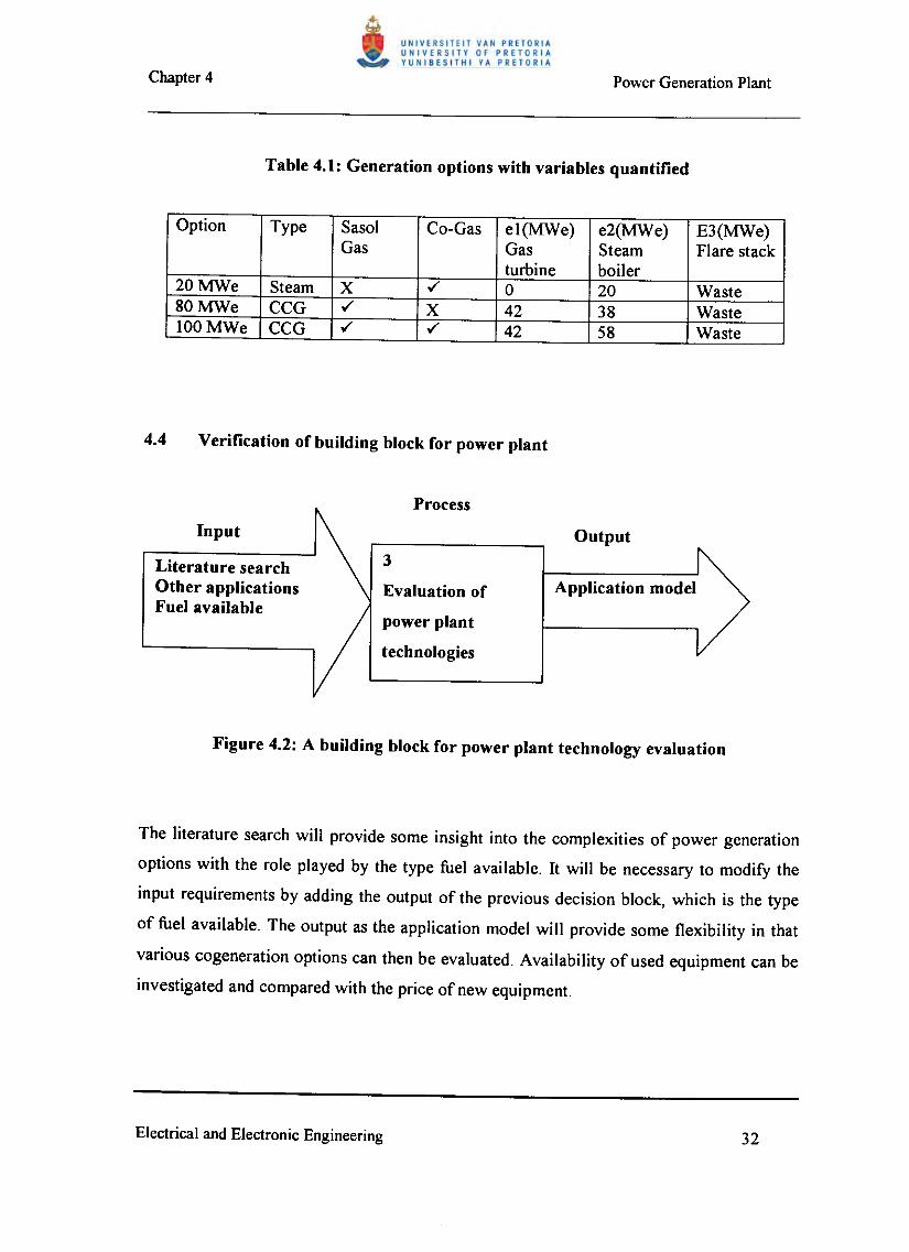
Option Type Sasol Co-Gas el(MWe) e2(MWe) E3(MWe)Gas Gas Steam Flare stack
turbine boiler20MWe Steam X ./ 0 20 Waste80MWe CCG ./ X 42 38 Waste100MWe CCG ./ ./ 42 58 Waste
Literature searchOther applicationsFuel available
power plant
technologies
The literature search will provide some insight into the complexities of power generation
options with the role played by the type fuel available. It will be necessary to modify the
input requirements by adding the output of the previous decision block, which is the type
of fuel available. The output as the application model will provide some flexibility in that
various cogeneration options can then be evaluated. Availability of used equipment can be
investigated and compared with the price of new equipment.

Where cogeneration plants are concerned, plant capacity is generally dictated by the local
heat demand, and manufacturers have indicated that they can offer cost effective
cogeneration plants, which will make maximum use of the primary energy source.
The information obtained with the conclusion of building blocks 1 to 3 would provide
sufficient information to give a clear indication of the power plant configuration and
whether it is a technically feasible option. The output of the building block on gas
evaluation is an essential input element to narrow down on the power plant configuration.
The financial aspects will now become more relevant and one can start to investigate the
flexibility of the operation and the optimisation of the real time pricing tariff.

Financial aspects will now be of importance as to how the proposed cogeneration plant can
be optimised to reduce electricity cost and to improve efficient utilisation of energy
available. Knowing that the opportunity exists for possible cogeneration implementation,
this chapter will investigate the RTP tariff whilst production targets must be maintained or
improved. Also the basic principles of an excel model, developed as part of this
investigation, will be discussed for use of the case study, with different production profiles
(RTP adapted).
RTP has been used successfully by utilities as a Demand Side Management (DSM) tool.
Significant load shifting out of peak periods has been achieved for these utilities while
customers have been able to profit from increased production at times of low prices. These
international experiences have been repeated by the South African electricity market,
where it has been clearly demonstrated that customers, who participate actively in the
dynamics of the product:
(a) Use significantly more electricity during system unconstrained periods and
(b) Shift significant load out of peak periods, as signalled by the real time price.
Prices do not vary continuously as the name may suggest. For practical reasons, pnce
levels are fixed for short discreet time periods, typically one hour. The day ahead posting
of hourly prices for the next day has become the industry standard, since few customers are
able to effectively respond with shorter notice.

RTP is a pricing methodology that exposes customers' consumption decisions to the short-
term value and availability of electricity. This results in the desired DSM behaviour of
RTP customers. Since the implementation of such a pilot project at a gold mine, Western
Deep Levels has proven the benefits to both the utility and the consumer by shifting loads
of up to 70MW and achieved a 2% reduction on the electricity bill, [23].
The objectives of the RTP product is to stimulate optimal customer behaviour through
dynamic price signalling which includes:
b) Increased energy sales (and hence net contribution) when the system IS
unconstrained, as reflected by low prices.
d) Reduced operating cost resulting from not having to start up more expensive units
to supply short peak loads.
e) Improved customer service, through lower overall average pnces and more
customer choice.
The philosophy of RTP is rooted in the principle of signalling to customers the dynamic
real time value of electricity, which will dictate the customer behaviour. Due to being the
only pilot tariff in South Africa, both the utility and the customer need to be protected.
Revenue neutrality will be maintained with respect to the previous pricing structure, when
the customer's load and load profile remains unchanged after conversion to RTP. Only
through load shifting or demand side management will it be possible for the customer to

reduce the average cost of electricity. The requirement for revenue neutrality will be
individualised at customer level, to prevent customers from being advantaged merely by
changing to RTP.
The historic load profile of the customer, which is known as the Customer Baseline Load
(CBL), is the fixed reference on which the calculation of fixed charges and revenue
neutrality will be based at the time of conversion. The CBL is therefore, by definition, "the
load profile that can reasonably be expected without behaviour modification (due to
RTP)".
The utility requirements are to use twelve-month continuous historical hourly data for
calculating the CBL, except if agreed to by both utility and consumer.
The CBL rate is calculated for a 30-day month and a 3 I-day month. February is always
treated as a 30-day month. The CBL charge is calculated using the following equation:
CBLcharge = ( Drale +Er•Ie). (1- Vdiscount)' (I+ Ssurcharge )24· days· Lf
Lf= EMD· 24· days

CBL charge c/kWh
Demand rate in c/kVA
Energy rate in c/kWh
Total energy consumed for the number of days
Maximum Demand in kVA
Load factor for applicable month (3D-day month or 31-day month)
Voltage discount
Transmission surcharge
CBLcharge
Drate
Erate
E
MD
Lf
The measured CBL shall be adjusted to reflect the shift in weekends and public holidays
and known events that have caused the recorded profile to deviate from the normal, may be
adjusted accordingly.
This RTP option has a two-part structure, namely the Access charge and the RTP Load
charge. The energy supplied at the CBL profile is priced at the customer's normal pervious
tariff and becomes a commitment of the customer. The customer therefore ..:.ommitsto pay
the utility for this amount of electricity, whether it is used or not. This mechanism
guarantees the utility's revenue requirements and also protects the customer against
exceptionally high prices.
The customer's actual energy consumption for every hour is measured and compared to the
CBL. The difference between the CBL and the actual consumption, measured for every
hour, is the RTP Load. If the actual load is greater than the CBL, the difference is the
Additional Load (AL). If the CBL is greater than the actual load, the difference is the
Reduced Load (RL). The AL is charged for at the RTP rate including the profit adder. The

RL is charged for at the RTP excluding the profit adder. The customer is effectively
refunded at the RTP rate excluding the profit adder for the energy not consumed below the
CBL.
BC
MR
AL =RL =RTPI =
RTP2 =
The Basic Charge. The BC is taken as the same as for the previous tariff.
Monthly Rental. The MR is taken as the same as for the previous tariff.
Any capital expenditure to switch to RTP will be included in the MR.
The Access Charge. This Access Charge is a commitment from the
customer, Richards Bay Minerals, to purchase the electrical energy under
the customer base load (CBL). The Access Charge is charged at the CBL
rate.
The Additional Load.
The Reduced Load.
Real-time Price including the profit adder.
Real-time Price excluding the profit adder.
The organisation that will be evaluated in the case study is on Nightsave tariff, it seems to
be in order to give a brief description thereof This tariff consists mainly of two
components, maXImum demand (kVA) and active energy charge (kWh). Maximum
demand is only payable during on-peak time periods where active energy is charged for the
total usage.

Weekdays consist of on-peak period from 06hOO to 22hOO, during which time period the
highest maximum demand will be recorded for payment at the end of the month. The rest
of the week day including weekends and public holidays are considered as off-peak time
periods where only the authorised connected load values as stipulated in the contract are
the maximum demand limit.
This tariff evaluation model was developed as a tool, in a spreadsheet environment, to
assist with the evaluation of the potential benefits through changing the load profile to
optimise the RTP tariff The following assumptions were made:
No seasonal loads were considered due to the nature of the operation, which was
also applicable for weekdays, where nightsave tariff was used.
Monthly CBL profiles were calculated for weekday and weekend.
CBL values for weekdays were calculated by using average hourly values for all
weekdays.
Weekends and holidays were treated the same as it was seen as "off-peak" periods.
For this application only seven-month historic data was used, with utility's
agreement.
The average weekday RTP rates were calculated for weekdays and weekends, from daily
schedules provided from the utility. Only the weekend values are shown for demonstration
purposes in Figure 5.1. The rates are sorted in an ascending order (random hours), which
will be used to construct the new profile based on the history to obtain the same energy
area.

1000
9.00
8.00
7.00
elk6.00
Wh S.OO
4.00
3.00
2.00
1.00
0.00
00 00 00 00 00 00
With the average RTP prices available, the new profile can now be constructed based on
the previous operational data and profile. The new profile will then be constructed by
placing the highest obtained load at the specific time of the lowest price for electricity. The
new profile will then be fitted on the CBL graph and an example is shown in Figure 5.2.
-CBL--JAN'99 WKED CBL
75000
~ 8 8 8 8 ~ 8 8 8 8 ~ 80 •••• .;.; r:-: ~ ~ .;.; t 2S - ••••0 0 0 N N
Hours

Evaluation of
electrical
tariff structures
Literature searchOther applications
The input requirement indicates that a close relationship with the utility may be an
advantage. This will provide you firsthand information on the tariff structures available
and perhaps pilot projects. Careful evaluation of the electricity load profiles should give
some indication on the load flexibility to apply demand side management and utilise any
additional capacity in low price periods. Using the same production kWh area should
provide some confidence on the possible success during tariff changes.
The RTP objectives set by the utility provides both parties with potential benefits and
savings. The tariff change might be restricted to specific utility conditions that should be
clarified in advance to assist with realistic evaluations. Investigation of the CBL profile
shows a large difference between on-peak and off-peak values, which indicates that
flexibility exists to to apply DSM. The effect of this DSM should be evaluated in terms of
production requirements. It is important to note the maximum RTP price on average was
about 9c1kW, which now can be compared to the specific plant's average cost to give an
indication of the expected change.
At this stage of the evaluation process, there should be a clear indication on whether a
cogeneration plant is an option or not. This chapter will give some insight into the
fundamentals of total economy for such an investment.
Producing energy with a cogeneration plant involves several cost groups such as
initial investment, capital, fuel, operations and maintenance. Achieving the lowest
total energy cost is therefore the sum of a correct investment in a reliable
technology/supplier and the organisation of all operational activities in an optimum
manner.
The Life Cycle Costing (LCC) method is normally used to determine the total
economy of a system under development. LCC requires the identification of all
potential costs, from plant concept to full operation. The true LCC is monitored
throughout the lifetime of the system. More than 60% of such a product's LCC is
generated during actual operation; many of an operator's daily decisions affect the
true LCC. Therefore, the operations phase is the most important from a total economy
point of view. LCC is not just a measurement and decision tool, but rather means a
constantly improving the effectiveness of maintenance that should be built into the
operational system.

Although capital cost represents the initial cost or investment for erecting and
maintaining a cogeneration plant, the most important factor is fuel costs. Changing the
fuel costs requires either changing the fuel type or improving fuel consumption.
The most common indicators used to compare mutually exclusive projects are simple
payback, internal rate of return (IRR) and the net present value (NPV).
Net present value and present value (PV) have to be understood before IRR can be
explained and the information is available in various financial textbooks of which [24]
is only one. The present value of an investment is the value of all the investment's
future payments or savings discounted to today's money. Discounting is done as
follows:
r= The discount rate and
n= number of years starting at 1
The present value of savings generated by a project is calculated by adding each tear's
discounted savings. Thus two factors are arbitrary in the present value calculation: the
discount rate and the lifetime of the project. The present value calculation is defined
as:
The basic rule is is that an investment is profitable if its NPV is larger than zero and
the IRR should be higher than the interest rate for borrowing the money.

There are various commercial packages or systems available for feasibility analyses
for power plant or cogeneration projects such as the "Feasibility Calculator" from a
company by the name Wartsila [25], or the one that will be used in this study which
was developed by a company Duke Engineering and Services Africa, Inc. (DE&S).
In order to model the CCG plant, it would be necessary, depending on the model, to
make certain assumptions depending on the specific requirements on each case. All
the parameters under the headings "Financial" and "Technical" are inputs with the
output parameters under the heading "Outputs" For the purposes of this study, the
model will be considered an additional aid and will not be discussed in any detail. The
assumption is made that the outputs will be reliable based on results of previous
evaluations for other operations, which are still in service. The input parameters can
be modified based on the specific requirements. One of the important output
parameters that will have a direct influence on the tariff evaluation will be the total
cost for generation of energy (electricity).
In the previous chapter, the maximum value of the RTP cost was given as
approximately 9 c/kWh, which is 45 % less than the 13,12 c/kWh of the cost to
generate electricity with cogeneration. These costs should be compared with the
specific plant average cost on the existing tariff structure. This would clearly show the
potential with or without cogeneration. For instance, if the existing average cost is a
value between 9 and 11 cents, it will indicate some potential for RTP but will be
uneconomical to implement cogeneration.

Combined Power and Heat Model by DE&S
Financial Technical
Electricity Price 10.00 clkWh Availability 90 %Gas Price 12.70 R/GJ Load FactorsSteam Price R/ton Electricity 100 %Electricity Escalation 10.0 %/yr Steam 100 %Gas Escalation 10.0 %/yr Gas Turbine Power 45.0 MWe
Repayment Term 15 Yrs OutputsDepreciation Term 3 Yrs IRR -0.1 %Interest Rate 16.50 % NPV, 15%, 15 yrs -68.3 R millDebt-Equity Ratio -% Total Power 102.54 MWeManagement Fee -% Gas Consumption GJ/yr
3,621,610Tax Relief O&M Costs 5.5 R millCompany Tax 35.0 % Total Project Costs 113.3 R millSecondary Tax 12.5 % Installed cost per kW 1,620 R/kW
O&M Costs: GT [j.50 clkWhO&M Costs: ST 0.50 clkWhContingency Costs: GT - clkWhContingency Costs: ST - clkWh
1.01 clkWh8.34 clkWh3.77 clkWh
- clkWh13.12 clkWh
O&MFuel CostsInterest CostsContingency CostTotal Energy Costs
O&M = Operation and maintenanceIRR =Investment rate on returnGT = Generator turbineNPV = Net present ValueST = Steam turbine

The model discussed in Chapter 5, was improved to make provision for modelling the
use of a cogeneration plant to influence the load profile. The actual generating
capacity needed to be specified for specific hours over weekdays and weekend for the
time period selected. The decision as to when to schedule the cogeneration is directly
related to the price that electricity could be purchased from the utility. This means that
if the price for buying from the utility is cheaper than the price to generate electricity,
then the cogenerator will not be utilised. Outsourcing or selling is another option that
can be considered if there is a demand.
Input
Cogeneration size
Commodity prices
Business case
5
Evaluation of
financial aspects
Capital cost
Generation cost
O&Mcost
From figure 6.1 it can be seen that the input requirements which will dictate the
output parameters are clearly the cogeneration plant's generating capacity, with the
commodities being the price of electricity and natural gas. The business case will be
dependent on the financial status of the investor and his credibility. Money markets
such as capital funding and interest rates will have an influence.

There are clearly a few important aspects that will influence the decision for the
implementation of cogeneration. From the DE&S model one could see that the some
of the input parameters should have an impact on the total energy cost for
cogeneration and will be discussed next.
• Interest rate on the loan.
The higher the interest rates the less attractive the project due to a higher
generating cost.
• The existing price paid for electricity from the utility. If the electricity is cheaper
to buy from the utility, then more expensive cogeneration is not a viable option.
• The price of the natural gas from the utility depends on quantities required and if
distribution infrastructure exists.
• The actual type and power plant required will influence this commodity. The
information in the literature search has indicated that steam turbine cogeneration
capacities are relatively small. For energy intensive operations with high
maximum demands, low cogeneration plant capacities may not look so viable and
there might be the need to increase the cogeneration capacity. This can be
achieved by selecting a CCG which is dual-fired with higher efficiencies.
• The aspects should therefore be properly analysed to obtain sufficient information
to assist with the decision. Some of these aspects will be discussed with the
evaluation of the business case.
• The output parameters clearly indicate that the decision pending the outcome is
financially driven. This means that unless there are any potential benefits that will
result in efficiency improvement with cost savings, this project is not likely to be
implemented.

• From table 6.1 the IRR or NPV are both negative which indicate that the
cogeneration option is not viable at all. The IRR should at least be more than the
interest rate for borrowing the money.

This Chapter will consist of a case study, which will be conducted on a typical mineral
sands business with electric arc furnaces as part of the operation. The cogeneration
evaluation process will be used, whilst each of the building blocks defined, will be
verified.
Most of the world's titanium ore production starts from heavy mineral sands and a typical
process is shown in Figure 7.1.
The dredging mmmg process mmes the heavy mineral concentrate (HMC) which is
transported to the mineral separation plant (MSP), where the HMC is separated into by-
products, rutile and zircon, with ilmenite as roaster feedstock and some tailings that are
returned to the dunes. The roaster treats the ilmenite, which is then fed to the smelter.
Anthracite is bought in and will be treated in the char plant to change the chemical
composition thereof The ilmenite from the roaster and the treated anthracite are then fed
into the smelter. The smelter output results in cast iron, which is transported to the iron
injection plant for treatment and casting. The titanium dioxide (Ti02), in coarse form is
then transported to the slag plant for crushing, milling and screening. The pig iron and the
slag are then ready for shipment to local and international customers.
The metallurgical process for removing iron from ilmenite is based on slag formation in
which the iron is reduced by anthracite or coke to metal at 1200-1600 degree Celsius in an
electric arc furnace, and then separated. Titanium free pig iron is produced together with

slag containing 70-80 % Ti02 (depending on the ore used) that can be digested with
sulphuric acid because they are in titanium and low in carbon. Raw materials of this type
are produced in Canada by Quebec Iron and Titanium Corporation (QIT), in South Africa
by Richards Bay Minerals (RBM) and to a smaller extent in Japan by Hokuetro Metal and
Tinfos Titan and Iron in Norway and only recently Namakwa Sands South Africa. The raw
materials for Ti02 production include natural product such as ilmenite, leucoxenene and
rutile [26].
The process is now evaluated by using the building block concept as illustrated in Chapter
2, of which the first step is to determine the energy inputs and outputs to and from the
plant. Useful energy sources identified consist mainly of electricity, anthracite, gas and
fuel for standby or emergency conditions. Although this is an energy intensive electricity
type operation, carbine monoxide (CO) gas is produced as a furnace off-gas which is used
by some of the primary and secondary operations with excess being flared (burnt) and
treated as waste.

DredgingMining
OperationsHeavy Mineral
Concentrate
MineralSeparation
Plant
Rutile& Zircon
Course TitaniaSlag
IronInjection
Plant
TitaniaSlag

Elec-tricity
DredgingMining
Operations
ElectricityFuelCO gasAnthracite
MSPRoaster
Char Plant
ElectricityFuelco gas
Iron InjectionSlag Plant
The process is now evaluated in terms of the energy sources for the inputs and outputs and
is structured in a simplistic form as useful energy. In the process and useful energy out as
described in Figure 7.2, which is summarised in building block form as illustrated in
Figure 7.3.

• Electricity• Fuel• Anthracite• Gas
Plant operations&stockpiles
• Furnace wastegas
• Heat
It will be useful to have an intimate knowledge of the specific operation, being evaluated,
as this will speed up the process and provide more comprehensive information. The
following information on the energy input parameters are:
Electricity. Imported from the local utility with the electric arc furnaces as the main
consumer that produces the outputs, namely heat and furnace waste gas
Anthracite. This is commercially obtained and when treated, it becomes part of the
furnace feed stock, which contributes to the CO gas production levels.
Gas. Carbon monoxide (CO) gas produced by the furnaces. Some of the gas is
distributed to other parts of the production for process heating and drying
and the rest is burnt and treated as waste, which can be used for
cogeneration.
Fuel. This is consumed in relatively small quantities of diesoline, which is mainly
used for emergency or abnormal conditions.

As previously mentioned, the CO gas is treated as waste and is burnt into the atmosphere,
which is definitely energy wastage.
Due to the nature of the operation, excessive heat is generated but is maintained within the
firewalls of the furnaces. This heat and possible uses will not be discussed here, but a
recommendation will be made based on the potential.
Furnace power levels and CO gas measurement results showed almost a 100% correlation
with relative steady production conditions and are illustrated in Figure 7.4. The fact that
the process heating and drying is independent of the furnace feedstock is due to sufficient
stockpile capacity available for a relative long duration. This provides some flexibility that
allows individual plants to vary the production profile (maintenance, breakdowns, etc).
Plant design information provided information to determine the internal CO gas
consumption for average and maximum conditions.
6171990:00 6171990:00 7m99 0:00 8171990:00 9171990:00 100199 0:00 11n199 0:00
I-FCEMVV- - - COGAS(X2)IFigure 7.4: Furnace power (kW) correlation with CO gas production (NmJ
)

These values were used to simulate the minimum and maximum CO gas quantities, which
will be flared, thus giving an indication of the flow pattern and are illustrated in Figure 7.5.
Various Gas samples were taken for Composite analyses by a reputable laboratory which
provided the gas content and energy levels as per the proposed layout as required by Table
3.1 in Chapter 3. This is sensitive information that will not be divulged here and an
assumption from a text book will be made on the energy content as being 11.79 MJ/Nm3
[27], for CO gas.
,-. I':'!. .11"'. ~ ~.i. . .~ -.. ~.~~! ~ I-! : I :; •.; 1
I- I'I I' Hi.!o" _'. . .':I. • .!II" •: i, .~. I, !t '.'. •• ;
I. •• " i~) I
..~30000E
o99/07/05 99107108
DateI -MtN FLARE •• MAXFLARE
The input parameters consisting of measurement analysis and sampling have provided the
information required as an output and are therefore correctly identified.
On evaluation of Figure 7.5, one can see that the CO gas volumes vary between 0 and
almost 50 000 Nm3. For safe turbine operation it is clear that the minimum gas for safe
turbine operation can be taken as 20 000 N m3.
The information obtained and discussed in Chapters I and 3 have indicated that electric
furnace waste gas is very dirty and should be treated by means of bag-houses and
scrubbers.
The laboratory analyses would be able to provide this information, but being sensitive, an
assumption has been made based on data obtained from a textbook being 11.79 MJ/Nm3.
[27].
The information obtained from Figure 7.5 clearly shows that a maximum value of between
40 - 50 000 Nm3 I hr can possibly be used for cogeneration. Indication then is that an
additional make-up fuel would be required to smooth out the erratic profile to prevent
damage to the turbine. Based on the assessment made to safely use the minimum value of
20 000 Nm3/hr, the generating capacity can be calculated for the type of technology
selected. For the next discussion and explanation of the power plant process flow model,
Figure 4.1 from Chapter 4 is repeated here as Figure 7.6.

...••.....•..~~ .1 ~~.2 Production Pr
Load 1 .3 L
~r VENT ~NATURAL JCKS fLARE
STACK OPERATIONA•...OAS GAS STEAM HEATINGTURBINE EXHAUST ••. TURBINE ~ ANDJIll" V'l POWER GASES •••. POWER FURNACES
PROPOSE[ DRYINGPLANT PLANT PROCESS
.4 •• otrgn ~..~ H~,Production
MEllluMPRESSURE
CO GASCOMPRESSORS
S~,
HIGH PRESSURE"-CO GAS
COMPRESSORS
In this configuration the CO gas from the Flare stack is utilized as the main fuel source.
Natural gas or oil will be used as a top-up and the gas is combusted in a gas-fired boiler.
Steam is then raised and a steam turbine is driven, resulting in 21,55 MWe generating
capacity. This is illustrated in Table 7.1, where the tick ( ~ ) means CO gas will be used,
with e2 equal to 21 MWe electrical generation into the utility busbar. With zero electricity
generated with the CCG, which is indicated with the X.
= Volume of gas x CV x k x efficiency (7.1 )
= 20 000 Nm3/hr x 11,79 MIl Nm3 x 0,277 MW x 0.33 pu
= 21,55 MWe
= Conversion factor of277,8 kW equals to 1Glib
= Megawatt electrical
= Nominal cubical metre
where k
MWe
Nm3
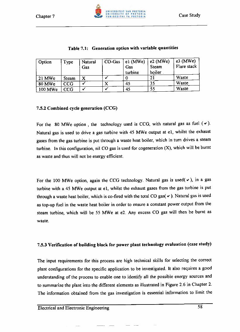
Option Type Natural CO-Gas el (MWe) e2 (MWe) e3 (MWe)Gas Gas Steam Flare stack
turbine boiler21 MWe Steam X ./ 0 21 Waste80MWe CCG ./ X 45 35 Waste100MWe CCG ./ ./ 45 55 Waste
For the 80 MWe option, the technology used is CCG, with natural gas as fuel (II).
Natural gas is used to drive a gas turbine with 45 MWe output at el, whilst the exhaust
gases from the gas turbine is put through a waste heat boiler, which in turn drives a steam
turbine. In this configuration, nil CO gas is used for cogeneration (X), which will be burnt
as waste and thus will not be energy efficient.
For the 100 MWe option, again the CCG technology. Natural gas is used( II), in a gas
turbine with a 45 MWe output at el, whilst the exhaust gases from the gas turbine is put
through a waste heat boiler, which is co-fired with the total CO gas( II ). Natural gas is used
as top-up fuel in the waste heat boiler in order to ensure a constant power output from the
steam turbine, which will be 55 MWe at e2. Any excess CO gas will then be burnt as
waste.
The input requirements for this process are high technical skills for selecting the correct
plant configurations for the specific application to be investigated. It also requires a good
understanding of the process to enable one to identify all the possible energy sources and
to summarize the plant into the different elements as illustrated in Figure 2.6 in Chapter 2.
The information obtained from the gas investigation is essential information to limit the

wide choice of options on the various power plant configurations. From a systems point of
view, it is shown that the relationship between these two building blocks, namely gas
evaluation prior to power plant evaluation is essential.
Although the utility requires a 12-month historical database for CBL calculations, it was
agreed between consumer and utility to use the seven-month history in this case. The
motivation for this was clearly due to a more aggressive approach towards nightsave, with
a considerable reduction in maximum demand during on-peak period.
As indicated in Chapter 5, the CBLs were calculated for weekdays and weekends
separately. With the objective to use the same area under the historic load profile, the new
profile is now constructed by allocating the highest load value to the cheapest hour for
each month.
The new profile (NP) is then fitted on the CBL graph as illustrated in Figure 7.7. For this
evaluation, with the assumptions made, only the difference in load, AL and RL is of
importance and will be used to calculate the price difference.
The results, with the RTP prices applied to the AL and RL values are illustrated in Figure
7.8. The cost benefits are summarized in Table 7.2, with the detailed spreadsheets for each
month's weekday and weekend, attached as Appendix A.

WEEKDAY CBL WITH RTP PROFILEJAN 1999
ooסס10
95000
90000~ 85000.l<: , -CBL
80000 ,•• NEW
PROFILE75000
700000 0 8 0
~0 0 0 0 0 0 0C? C? C? C? C? C? C? C? C? C?•....• M V"i e- o.. •....• M II"l e- o.. •....• M
0 0 0 0 0 •....• •....• •....• N N
Hours
COST DIFFERENCE (NEW PROFILE - CBL)JANUARY 1999
0 0 0 0 0 0 0 0 0 0 0 0<? 0 0 0 0 <? 0 0 0 0 <? 0....• ,:,.; Vi r-: 0; ....• ,:,.; Vi r-: 0; ....• ,:,.;0 0 0 0 0 ....• ....• ....• ....• ....• N N
400.000
0.000
"'='c -200.0000:1~
-400.000
-600.000
-800.000

Monthly Jan Feb Mar Apr May Jun Jul
'99 '99 '99 '99 '99 '99 '99
Weekdays
Number of days 21 20 23 19 21 21 22
Cost Difference (NP-CBL )(R * 1000) (1) 4 0 (3) (2) (1) 2
Additional cost/(saving)(R * 1000) (23) 79 1 (61) (51) (22) 33
Weekends
Number of weekends 5 4 4 4 5 5 5
Cost difference (NP-CBL)(R) 10 4,6 (4,5) (4,7) (1,5) (1,6) 4,5
Additional cost/( -saving)(R * 1000) 0 19 (18) (19) (8) (8) 23
Cost/(saving)(R * 1000) (23) 97 (17) (80) (58) (30) 56
Total cost/saving(R * 1000) (55) Sum of monthly values
Annual cost/( saving)(R * 1000) (94,1) Predicted annual cost
The summated cost values for the seven months of the year show a saving ofR54, 913.07,
which can be interpreted as R 7,844.72 saving per month which will then give a total
predicted saving ofR 94,136.69 per annum. This demonstrates then, with the capability to
adapt to the RTP tariff, that there will be a potential saving if the same production outputs
are maintained.
Inspecting the load profile in Figure 7.7, indicates that the plant does have the capability to
adapt to the RTP. This is supported with the ± 16 MW difference between maxi mum and
minimum values recorded, which is almost a 16 % variation.

From the three types of cogeneration plant options in the previous chapter, the 100 MW
CCG provides the best flexibility to conduct financial evaluations with the DE&S model,
for capital investment and the potential tariff evaluation with cogeneration. The 80 MW
CCG plant does not adhere to the requirement of the initial condition set, which was to
utilize the CO gas that is treated as waste, and is therefor disqualified and will not be
discussed. The steam generation system has no flexibility to evaluate different scenarios
and it was also identified as being inefficient and too expensive. For this case study, only
the 100 MW CCG will be discussed.
From the discussions on the financial model illustrated in Chapter 6, it was identified that
the existing price paid for electricity will play an important role in the decision-making
process. With electricity that is cheaper to buy from the utility, cogeneration would not be
a viable option.
The following assumptions made for this case study produced the information as illustrated
as Table 7.3, which will be further discussed:
• The banker is so kind as to extend the repayment term from 15 to 20 years and the
interest rate dropped as low as 8 %, due to an improved economy.
• The Panda gas fields have been explored and the natural gas is available at R6, 00 per
GJ.

Although simple payback is the most common method of companson, the major
disadvantage is that it does not take into account the savings after the payback period. On
the other hand, the present value of the savings generated by a project is calculated by
adding each year's discounted savings. The NPV is then simply the present value of
savings minus the investment cost, which looks very good at more than R 170 million over
15 year period.
This high NPV is obtained due to the large difference in electricity price from the utility
(13 clkWh) and the relative cheap cost for generating (5,98 c/kWh). Another contributor is
the low gas price. Remember that the steam generation portion is 55 % of total electricity
generated, which make this portion of electricity generation, very cheap.
The IRR, which is the discount rate that yields a zero NPV, is 40,6 %, which is
exceptionally good. This rate is a lot higher than the interest rate at which this money will
be borrowed. Also some companies will consider investing at IRR rates as low as 15 %.
Thus to put this in other financial terms means that this is relatively cheap money to
borrow for such an investment.

Combined Power and HeatModel by DE&S
Financial Technical
Electricity Price 13.00 clkWh Availability 90 %Gas Price 4.39 R/GJ Load FactorsSteam Price R/ton Electricity 100 %Electricity Escalation 10.0 %/yr. Steam 100 %Gas Escalation 10.0 %/yr. Gas Turbine Power 45.0 MWe
Repayment Term 20 yr. OutputsDepreciation Term 3 yr. IRR, BlAT 40.6 %Interest Rate 8.00 % NPV, 15%, 15 yr. 170.5 R millDebt-Equity Ratio -% Total Power 102.54 MWeManagement Fee -% Gas Consumption GJ/yr.
3,621,610Tax Relief O&M Costs 5.5 R millCompany Tax 35.0 % Total Project Costs 113.3 R millSecondary Tax 12.5 % Installed cost per kW 1,620 R/kW
O&M Costs: GT [J.50 clkWhO&M Costs: ST 0.50 clkWhContingency Costs: GT - clkWhContingency Costs: ST - clkWh
O&MFuel CostsInterest CostsContingency CostTotal Energy Costs
1.01 clkWh2.88 clkWh2.09 clkWh
- clkWh5.98 clkWh
Inspection of the monthly RTP average prices, for both weekdays and weekends show that
there is plenty opportunity to run this 100 MW cogeneration plant. The scheduling of the
cogeneration plant is illustrated in Figure 7.9, where the new profile is plotted with the
CBL (January 99 weekday as an example). Due to operational constraints on the utilization
of the cogenerator plant, it is recommended to perform two separate case studies for
demonstration purposes.

ooסס12
ooסס10
ooסס8
ooסס6
~ ooסס4ooסס2
0
OOסס2-ooסס4-
WEEKDAY CBL WITH NEW PROFILEJANUARY 1999
• .~ ~..- :
: :• :I · I
I I• •I I
I I• :I I
I I• •I :. . . • I • . . . . I • . .. . . ..•. - - - - .I
" - ~
--Fixed CaL WdAvg.
• • 'NP-COGEN
~ 8 0 0 8 0 0 0 0 0 0 09 0 9 0 0 0 0 0 0
M V'\ r:..: Q\ ..• M V'\ r:..: Q\ M0 0 0 0 0 ..• ..• ..• ..• ..• N N
Hour
This is the more theoretical approach, where cogeneration will be operational at all hours
where RTP price is 6 c/kWh and more. From Figure 7.9, it can clearly be seen that
electricity will be exported during their operational period.
The cost benefits are summarized in Table 7.4 with the detailed spreadsheets for the
monthly weekday and weekends attached as Appendix B. This evaluation supports the
DE&S results with a clear indication that this will be a good business proposition.

Monthly Jan Feb Mar Apr May' 99 Jun Jul
'99 '99 '99 '99 '99 '99
Weekdays
Number of days 21 20 23 19 21 21 22
Cost Difference (NP-CBL) (73) (68) (72) (75) (75) (73) (71)
(R·l000)
Additional cost!(saving) (1,539) (1,365) (1,659) (1,432) (1,566) (1,537) (1,554)
(R·l000)
Weekends
Number of weekends 5 4 4 4 5 5 5
Cost difference (NP-CBL)(R)
Additional cost! (192.86) (135,83) (172,49) (173,04) (200,54) (201,12) (170,08)
(-saving)(R ·1000)
Cost!(saving)(R·IOoo) (1,731) (1,501) (1,831) (1,605) (1,767) (1,738) (1,724)
Total cost/saving(R·l 000) (11.897) Sum of monthly values
Annual cost!(saving)(R·1 000) (20,396) Predicted annual cost
From an operational point of view, the preference would be to run continuously over a set
period, with the limitation that RTP should not be more than 10 % less than cogeneration
price and it should run for a minimum period of 4 hours. This limitation is overcome with
the scheduling of the cogeneration as illustrated in Figure 7.10. The cost benefits are
summarised in Table 7.5, with the detailed spreadsheets attached as Appendix C.
Comparing the two cases with each other, it seems that the more practical approach (Case
2), result in additional savings, which is, from a machine maintenance perspective
advantageous for the machinery and equipment.

WEEKDAY CBL WIlli NEW PROFILEJANUARY 1999
120000oo0סס18000060000
~ 4000020000
0-20000-40000
--' Il;~ r--- ., ,,,I
I I
II II, ,, ,. . . . . . . . . . ,. . ., - ..- - - ~ ~ .'.- - - - -.
--Fixed CBLWdAvg.•• - NP-COGEN
Monthly Jan Feb Mar Apr May' 99 Jun Jul
'99 '99 '99 '99 '99 '99
Weekdays
Number of days 21 20 23 19 21 21 22
Cost Difference (NP-CBL) (95) (90) (94) (97) (96) (95) (92)
(R*I000)
Additional cost!(saving) (1,988) (1,793) (2,151) (1,839) (2,015) (1,986) (2,025)
(R*I000)
Weekends
Number of weekends 5 4 4 4 5 5 5
Cost difference (NP-CBL)(R)
Additional cost! (131,99) (100,61) (123,80) (124,35) (139,67) (140,26) (109,21)
(-saving)(R *1000)
Cost!(saving)(R *1000) (2,120) (1,893) (2,275) (1,963) (2,155) (2,127) (2,134)
Total cost!saving(R *1000) (14,666) Sum of monthly values
Annual cost!(saving)(R*1000) (25,143) Predicted annual cost

The inputs are market driven, which cannot be influenced by the specific plant and the
immediate environment. This means that the cogeneration capacity is dependent on the
plant infrastructure and the availability of fuel, which cannot easily be changed without
capital expenditure to maintain at least the same output. The commodity prices are
dependent on the economic climate and also cannot be changed by the operation. This then
indicates that it will be necessary to clearly define a business case, which can then be
evaluated, based on the outcome. Typically the business case can be approved with an IRR
of 30 % or more. This DR&S financial calculator provides sufficient information to assist
the feasibility of such a capital-intensive project. One of the more important output
parameters of this process is in fact the generation cost of electricity, dependent on the
plant size specified by the customer. This information then needs additional manipulation
to determine how this is going to be used with DSM for energy efficiency improvement.
The outcome of this building block should be sufficient in providing information to make
conceptual decisions.
The second part of the financial evaluation is in fact the results of the spreadsheets
developed for this study. The outcome is referring to the difference in cost and not actual
values, which means a saving or additional cost. The flexibility to re-schedule the
cogeneration facility is very useful and the optimum solution can be obtained.
This provides one the tool to test various options without any expenses and provides
information on the proposed load profile for he specific organization.
The impact of the process as a system can have major financial and technical implications
that need to be discussed. The processes identified for a cogeneration system can each be
investigated individually and at random, but will confuse the issue.
This will have certain disadvantages in that it is possible to obtain a lot of data,
information, technical parameters, etc, which may not be relevant to the specific
cogeneration option being investigated. The design process confirms that the first and most
important process is in fact the plant, which should be evaluated in terms of the
opportunities that exist for cogeneration use. The energy source (gas & fuel), should then
be evaluated to determine the type of fuel available to make it easier to select the
technology for the application.
The information obtained from this two processes can then indicate the size and capability
of the cogeneartion plant, which will now be evaluated in terms of utilisation to manipulate
the tariffs. Again it is possible to obtain information on the tariff structures, but it will be
difficult to quantify without understanding the availability and energy contentwhich will
influence the cost directly.
This design process for cogeneration as a system provides a tool to guide one through the
steps required before making hasty decisions, which can be expensive if it is the wrong
decision.

In this chapter conclusions will be made to review to what extent the objectives set
were achieved. Recommendations will then be made on the possible use of this
methodology process for operations other than mineral sand businesses.
The main objective set was to create a methodology to evaluate the impact of load
scheduling, cogeneration and RTP on the energy cost of a typical titanium mineral
producer in the mineral sands industry. This objective was achieved by providing a
model in a spreadsheet environment, which converted the historical load profile to a
new load profile with definite cost saving potential, without applying any load
scheduling. The conversion of the historical energy area to a new load profile with
the same energy area, without any load scheduling is already a positive conclusion,
which indicates future potential with the use of load scheduling. The spreadsheet
environment developed for this study, shows that it is relatively easy to investigate
various scenarios without incurring any cost, which is an advantage.
The difference between the maximum and mInimum load values indicates that
flexibility exists to reschedule some load to obtain greater cost saving advantages.
The results obtained whilst cogenerating electricity during the higher priced periods of
the RTP, have showed that it can be very economical if external factors such as gas,
electricity price and interest rates on borrowing money are more favorable towards the

potential investor into cogeneration. Not only will the plant generate electricity for its
own needs but it will also be able to export.
With the addition of a cogeneration into the system, the load scheduling principles are
now enhanced. The cheaper electricity can now be imported from the utility whilst the
cogenerator will supply, when the utility price exceeds the cogeneration price to
generate electricity. This shows very high monetary values, which means lots of
potential cost savings.
The application of cogeneration in any industrial application is dependent on various
aspects, which were identified as processes in this study. For these processes, not all
the input and output parameters were measured and quantified. The focus was more
on whether sufficient information was obtained to proceed to the next process, or not.
The relationship of the building blocks was shown to be dependent on the availability
of information. This assisted with the decision-making process and some alternatives
could be eliminated without further investigation. This then confirms that the
relationship between the processes can be flexible, but they will influence each other.
This is confirmed to be a reliable system, which can be modified by adding or
reducing building blocks depending on the specific case study being evaluated. The
work done in establishing a methodology, provides guidance for the prospective
cogenerator who wants to invest such an installation
Intimate knowledge and a good understanding of operational processes will be a
definite advantage with the confirmation of the energy resources. One should
distinguish between the cost components and the application for the different energy
resources available to keep focused on the objectives set for the specific application.
In this study, CO gas was identified as a useful energy component which was burnt
and treated as waste, whilst there are a few other potential aspects, such as using the
heat generated by the furnaces, that needs further investigation for other applications.
The process described here for a titanium mineral process should be useful for
evaluating any other industrial plant because the process is energy focussed and most
industrial plants use relatively the same energy sources such as electricity, gas, fuel,
and steam.
The basic techniques identified here consist of theoretical calculations for which the
results are confirmed by means of field measurements. Again the focus here was gas,
but the technique should apply for any other type of energy source. The type of
equipment used for the field measurement should be reliable, accurate and suitable for
the application. The information obtained in this study was sufficient to confirm the
quantity and volumes available for cogeneration use.
This building block was strongly influenced by the outcome of the gas or fuel
investigation. Information disclosed in this section is very general and it excludes
most of the technical aspects for the implementation of a cogeneration plant.
Technical support and experience in the field of electricity generation are required,
which can be of assistance with the decision-making process but can also have a
financial impact on the selection of power plant equipment.

Again, a good understanding of the available tariffs from the utility is required. The
RTP tariff used in this study was not an official tariff and only selected pilot plants
were approved. The methodology applied in this study is reliable, but only relevant to
electricity consumers who have no seasonal load profiles, with flexibility to adjust
load. For such loads, the individual days will have to be profiled for further
evaluation.
The utility's requirement for changing tariffs is that it will be revenue neutral and
supports the methodology of only investigating the AL and RL. The assumption made
to ignore the profit adder in the RL component, proved to be acceptable, as it will
have very little impact on the outcome of this case study. The profit adder should be
incorporated where the difference between AL and RL is only marginal.
Commercial software packages are available and they make provision for inputs or
assumptions to suit the specific conditions and requirements. It is therefore necessary
to understand the basic operation of the system to enhance the level of confidence in
the results.
The results, without the assumptions, have indicated that the cost of cogeneration is
more expensive than the purchasing of electricity from the utility, which makes the
project not at all feasible. The program is flexible to allow "what ifs", to predict
possible changes. This 'what if' allows one to influence possible future scenarios and
predict an outcome. This is a very useful tool to have for financial evaluations on
power generation plant feasibility.

Equipped with information on the technology, capacity, capital cost, generating cost
of electricity and the business case, the influence thereof can be evaluated on the area
of concern. In this case, the optimisation of RTP was successfully investigated by
enhancing the load scheduling process with the availability of a cogeneration
capacity.
The simple process of measuring the outcome of each of the building blocks can be
further developed into an iterative process to improve the technique. The furnaces are
operating at very high temperatures and an investigation should be initiated to
determine the possible use of the heat energy. The software tools provided, used and
recommended in this study should be evaluated and tested for information available
on actual installations to increase the level of understanding and confidence.

[1] RB Anderson, "Cogeneration and Independent Electric Power Production",
pp5-9, Electron October 1993.
[2] K Moslehi, G. Hernandez, "Optimization of Multiplant Cogeneration System
Operation including Electric & Steam Networks". pp484--450, IEEE
Transactions on Power Systems, Vol 6, May 1991.
[3] A Kuwahata, H Asano, "Utility Cogeneration Game for Pricing Power Sales
and Wheeling Fees", pp1875-1879, IEEE Transactions on Power System, Vol.
9, No 4, November 1994.
[4] Bin-Kwie Chen, "Optimum Operation for a Back-pressure Cogeneration System
under Time-of-Use Rates", ppl074-1082, IEEE Transactions on Power
Systems, Vol. 11,N02, May 1996.
[5] M Mansour and C Davidson, "A Unique Cogeneration Application in a Large
Pulp Mill Electrical System". pp34--40, IEEE Industry Applications Magazine,
September/October 1997.
[6] RB Anderson. "A Survey of Cogeneration and Independent Power Generation
World-wide and the Potential for its App1icationin South Africa," Final Report
No ED9013 to the Department of Minerals and Energy Affairs, April 1993.
[7] Keylink Eskom Customised Service for Key Custormers, Connect, pI 0,
November 1998.
[8] Electricite de France, "Clean Coal Technology", Energize, pp55-57,
NovemberlDecember 1997.
[9] Ron Rorich, "The Development of a National Air Quality Monitoring
Network", Energize, pp56-57, NovemberlDecember 1997.
[10] M Nkalaske, "Experience with application of NRS048 by the National
Electricity Regulator", 2nd Southern African Power Quality Conference in
Johannesaburg, 7 - 9 September 1999.
[11] OJ Erasmus, "New Paradigms for Managing Flicker Emission and Utility
Flicker Levels, 8th International Power Quality Applications Conference, Cape
Town, 9 -11 November 1998.
[12] Press release, "Cogeneration at Samancor's Meyerton Works", Engineering
News, 7 April 1995.

[13] GJ Delport, "Integrated Electricity End-use Planning in Deep Level Mines",
Thesis Submitted for PHD, University of Pretoria, Chapter 1 and 2, October
1994.
[14] "Systems Engineering and Analysis", BS Blanchard, WJ Fabrycky, pp256-318,
1981 by Prentice-Hall, Inc., Englewood Cliffs, New Jersey.
[15] TA Athey, "Systematic systems approach". 1982, Prentice Hall, Inc. Englewood
Cliffs, New Jersey.
[16] R Gusso & M Pucci, "Cogeneration combined cycle for Steel Industry Utilizing
Compressed BFG/COGILDG gas", Nuovo Pignone, SOA Seminar
Johannesburg, 1997.
[17] JF Douglas, 1M Gasiorek and JA Swaffield, "Fluid Mechanics," 2nd Edition,
Longman Scientific & Technical, 1986.
[18] Siemens Power Generation Publication Titled "Commitment to the future",
1994.
[19] Information from GE Power Systems, "Combined Cycle Technology - Past,
Present and Futue", Energize, p48, JanuarylFebruary 1998.
[20] Anton Rohrer, "Power Generation", ABB Review, Volume 3 1996 and
published as "Comparison of Combined Heat and Power Generation Plants"
pp23-26, Power International, May/June 1996.
[21] R Gusso, "Recent trends and development of gas turbine for combined cycles
and cogeneration", ppl-3, SOA Seminar Johannesburg, 1997.
[22] G Bonfiglioli, G Forconi, "Cogeneration with gas turbines for district heating
and industrial application, ppl-7, Nuovo Pignone - SQA Seminar
Johannesburg, 1994.
[23] Ken Cambell, "On line electricity savings at Western Deep Levels", pp6-8,
Vector May 1998.
[24] Calvin Engler, "Managerial Accounting", 3rd Edition 1993, pp718-731, Irwin,
Homewood, Boston.
[25] S Suvisaari, "Calculating feasibility of modernization projects", Energy News,
ppI6-19, Issue 2, 1998.
[26] F Habashi, "Handbook of Extractive Metallurgy", 1997, John Wiley & Sons,
NY ISBN3527287922, ppI129-1180.
[27] TD Eastop, A McConkey, "Applied Thermodynamics for Engineering
Technologist", pp580-590, 1978, 3rd Edition Longman Inc., New York

RTP 6 MONTH AVG. COST Cogen Fixed CBl Wd Av, NP-NOCOGEN NP-COGEN NP-CBl NP-CBlTIME c/kWh TIME c/kWh TIME c/kWh kW TIME kW kW kW TIME kW Diff Cost Diff (R)04:00 2.918 01:00 3.271 01:00 01:00 93367.755 94518.160 94518.160 01:00 1150.404 37.6303:00 2.955 02:00 3.081 02:00 02:00 93353.807 95594.642 95594.642 02:00 2240.835 69.0505:00 3.016 03:00 2.955 03:00 03:00 95198.321 96238.765 96238.765 03:00 1040.444 30.7502:00 3.081 04:00 2.918 04:00 04:00 95223.349 96344.649 96344.649 04:00 1121.300 32.7101:00 3.271 05:00 3.016 05:00 05:00 95324.829 96084.352 96084.352 05:00 759.524 22.9106:00 3.767 06:00 3.767 06:00 06:00 96555.758 94496.101 94496.101 06:00 -2059.658 (77.59)00:00 4.029 07:00 5.818 07:00 07:00 91631.479 88257.802 88257.802 07:00 -3373.677 196.29)23:00 4.652 08:00 7.115 08:00 08:00 90126.108 84913.650 84913.650 08:00 -5212.458 370.88'17:00 5.030 09:00 6.846 09:00 09:00 87912.010 86232.781 86232.781 09:00 -1679.228 114.97'22:00 5.195 10:00 6.584 10:00 10:00 86297.053 87101.908 87101.908 10:00 804.855 52.9916:00 5.243 11:00 7.113 11:00 11:00 83283.152 85756.306 85756.306 11:00 2473.154 175.9115:00 5.514 12:00 7.198 12:00 12:00 83381.360 84913.650 84913.650 12:00 1532.290 110.3018:00 5.608 13:00 7.260 13:00 13:00 83844.655 82690.099 82690.099 13:00 -1154.557 (83.82\07:00 5.818 14:00 6.226 14:00 14:00 83597.289 87137.202 87137.202 14:00 3539.913 220.3821:00 6.096 15:00 5.514 15:00 15:00 85449.384 88857.808 88857.808 15:00 3408.424 187.9414:00 6.226 16:00 5.243 16:00 16:00 86925.287 88893.103 88893.103 16:00 1967.816 103.1810:00 6.584 17:00 5.030 17:00 17:00 87001.202 89678.405 89678.405 17:00 2677.203 134.6709:00 6.846 18:00 5.608 18:00 18:00 88394.045 88654.865 88654.865 18:00 260.820 14.6311:00 7.113 19:00 8.745 19:00 19:00 88725.467 82531.273 82531.273 19:00 -6194.195 (541.68\08:00 7.115 20:00 8.978 20:00 20:00 89142.414 81018.023 81018.023 20:00 -8124.391 (729.45\12:00 7.198 21:00 6.096 21:00 21:00 89198.740 87225.439 87225.439 21:00 -1973.301 120.29\13:00 7.260 22:00 5.195 22:00 22:00 89056.438 89431.343 89431.343 22:00 374.905 19.4819:00 8.745 23:00 4.652 23:00 23:00 95205.075 93935.801 93935.801 23:00 -1269.273 (59.05\20:00 8.978 00:00 4.029 00:00 00:00 94787.968 94288.746 94288.746 00:00 -499.223 (20.11\
Additional cost/(saving)NP = New ProfileRTP = Real Time PricingWD=WeekdayAVG = AverageCOGEN = CogenerationCBL = Customer Base LoadDIFF = Difference
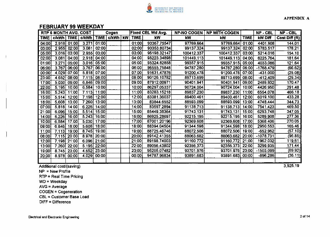
RTP 6 MONTH AVG. COST Cogen Fixed CBl Wd Avg. NP-NOCOGEN NP WITH COGEN NP -CBl NP-CBlTIME c/kWh TIME c/kWh TIME c/kWh kW TIME kW kW kW TIME kW Oiff Cost Oiff (R)04:00 2.918 01:00 3.271 01:00 01:00 93367.75547 97769.664 97769.664 01:00 4401.908 144.0103:00 2.955 02:00 3.081 02:00 02:00 93353.80734 99137.324 99137.324 02:00 5783.517 178.2105:00 3.016 03:00 2.955 03:00 03:00 95198.32147 100412.337 100412.337 03:00 5214.016 154.1002:00 3.081 04:00 2.918 04:00 04:00 95223.34898 101449.113 101449.113 04:00 6225.764 181.6401:00 3.271 05:00 3.016 05:00 05:00 95324.82858 99357.915 99357.915 05:00 4033.086 121.6406:00 3.767 06:00 3.767 06:00 06:00 96555.75848 94787.280 94787.280 06:00 -1768.479 (66.62)00:00 4.029 07:00 5.818 07:00 07:00 91631.47876 91200.478 91200.478 07:00 -431.000 (25.08)23:00 4.652 08:00 7.115 08:00 08:00 90126.10782 89713.699 89713.699 08:00 -412.409 (29.34)17:00 5.030 09:00 6.846 09:00 09:00 87912.00971 90401.941 90401.941 09:00 2489.932 170.4722:00 5.195 10:00 6.584 10:00 10:00 86297.05337 90724.004 90724.004 10:00 4426.950 291.4816:00 5.243 11:00 7.113 11:00 11:00 83283.15218 89837.230 89837.230 11:00 6554.078 466.1815:00 5.514 12:00 7.198 12:00 12:00 83381.36037 89400.461 89400.461 12:00 6019.100 433.2818:00 5.608 13:00 7.260 13:00 13:00 83844.6552 88593.099 88593.099 13:00 4748.444 344.7307:00 5.818 14:00 6.226 14:00 14:00 83597.2894 91138.713 91138.713 14:00 7541.423 469.5021:00 6.096 15:00 5.514 15:00 15:00 85449.38364 91743.131 91743.131 15:00 6293.748 347.0514:00 6.226 16:00 5.243 16:00 16:00 86925.28697 92215.195 92215.195 16:00 5289.908 277.3610:00 6.584 17:00 5.030 17:00 17:00 87001.20196 92369.608 92369.608 17:00 5368.406 270.0509:00 6.846 18:00 5.608 18:00 18:00 88394.04504 91344.598 91344.598 18:00 2950.553 165.4611:00 7.113 19:00 8.745 19:00 19:00 88725.46746 88072.506 88072.506 19:00 -652.962 (57.10)08:00 7.115 20:00 8.978 20:00 20:00 89142.41355 88063.682 88063.682 20:00 -1078.731 (96.85)12:00 7.198 21:00 6.096 21:00 21:00 89198.74003 91160.772 91160.772 21:00 1962.032 119.6113:00 7.260 22:00 5.195 22:00 22:00 89056.43802 92356.373 92356.373 22:00 3299.935 171.4419:00 8.745 23:00 4.652 23:00 23:00 95205.07482 93701.976 93701.976 23:00 -1503.099 (69.92)20:00 8.978 00:00 4.029 00:00 00:00 94787.96834 93891.683 93891.683 00:00 -896.286 (36.11)
Additional cost/(saving)NP = New ProfileRTP = Real Time PricingWD= WeekdayAVG = AverageCOGEN = CogenerationCBl = Customer Base loadDIFF = Difference

RTP 6 MONTH AVG. COST Coaen Fixed CBL Wd Ava. NP -NOCOGEN NP WITH COGEN NP -CBL NP -CBLTIME c/kWh TIME c/kWh TIME c/kWh kW TIME kW kW kW TIME kW Oiff Cost Oiff (R)04:00 2.918 01:00 3.271 01:00 01:00 93367.75547 96084.352 96084.352 01:00 2716.597 88.8703:00 2.955 02:00 3.081 02:00 02:00 93353.80734 96344.649 96344.649 02:00 2990.842 92.1605:00 3.016 03:00 2.955 03:00 03:00 95198.32147 95594.642 95594.642 03:00 396.321 11.7102:00 3.081 04:00 2.918 04:00 04:00 95223.34898 94518.160 94518.160 04:00 -705.189 (20.57}01:00 3.271 05:00 3.016 05:00 05:00 95324.82858 96238.765 96238.765 05:00 913.937 27.5606:00 3.767 06:00 3.767 06:00 06:00 96555.75848 94496.101 94496.101 06:00 -2059.658 (17.5900:00 4.029 07:00 5.818 07:00 07:00 91631.47876 87137.202 87137.202 07:00 -4494.277 (261.5023:00 4.652 08:00 7.115 08:00 08:00 90126.10782 81018.023 81018.023 08:00 -9108.085 (648.0617:00 5.030 09:00 6.846 09:00 09:00 87912.00971 88654.865 88654.865 09:00 742.855 50.8622:00 5.195 10:00 6.584 10:00 10:00 86297.05337 89678.405 89678.405 10:00 3381.352 222.6416:00 5.243 11:00 7.113 11:00 11:00 83283.15218 82531.273 82531.273 11:00 -751.879 (53.48'15:00 5.514 12:00 7.198 12:00 12:00 83381.36037 87225.439 87225.439 12:00 3844.078 276.7118:00 5.608 13:00 7.260 13:00 13:00 83844.6552 89431.343 89431.343 13:00 5586.688 405.5907:00 5.818 14:00 6.226 14:00 14:00 83597.2894 88893.103 88893.103 14:00 5295.813 329.7021:00 6.096 15:00 5.514 15:00 15:00 85449.38364 84913.650 84913.650 15:00 -535.734 29.5414:00 6.226 16:00 5.243 16:00 16:00 86925.28697 85756.306 85756.306 16:00 -1168.981 61.2910:00 6.584 17:00 5.030 17:00 17:00 87001.20196 86232.781 86232.781 17:00 -768.421 38.6509:00 6.846 18:00 5.608 18:00 18:00 88394.04504 82690.099 82690.099 18:00 -5703.947 (319.8611:00 7.113 19:00 8.745 19:00 19:00 88725.46746 93935.801 93935.801 19:00 5210.334 455.6408:00 7.115 20:00 8.978 20:00 20:00 89142.41355 94288.746 94288.746 20:00 5146.332 462.0612:00 7.198 21:00 6.096 21:00 21:00 89198.74003 88857.808 88857.808 21:00 -340.932 (20.7813:00 7.260 22:00 5.195 22:00 22:00 89056.43802 87101.908 87101.908 22:00 -1954.530 101.5419:00 8.745 23:00 4.652 23:00 23:00 95205.07482 84913.650 84913.650 23:00 -10291.425 478.7520:00 8.978 00:00 4.029 00:00 00:00 94787.96834 88257.802 88257.802 00:00 -6530.166 263.08
Additional cost/(saving)NP = New ProfileRTP = Real Time PricingWD = WeekdayAVG = AverageCOGEN = CogenerationCBL = Customer Base LoadDIFF = Difference

RTP 6 MONTH AVG. COST Cogen Fixed CBl Wd Avg. NP-NOCOGEN NP WITH COGEN NP -CBl NP-CBlTIME c/kWh TIME c/kWh TIME c/kWh kW TIME kW kW kW TIME kW Olff Cost Oiff (R04:00 2.918 01:00 3.271 01:00 01:00 93367.75547 90989.641 90989.641 01:00 -2378.115 77.8003:00 2.955 02:00 3.081 02:00 02:00 93353.80734 91022.149 91022.149 02:00 -2331.658 71.8505:00 3.016 03:00 2.955 03:00 03:00 95198.32147 92085.627 92085.627 03:00 -3112.694 91.9902:00 3.081 04:00 2.918 04:00 04:00 95223.34898 92800.806 92800.806 04:00 -2422.543 70.6801:00 3.271 05:00 3.016 05:00 05:00 95324.82858 91073.233 91073.233 05:00 -4251.596 128.2306:00 3.767 06:00 3.767 06:00 06:00 96555.75848 90724.932 90724.932 06:00 -5830.826 219.6500:00 4.029 07:00 5.818 07:00 07:00 91631.47876 86029.838 86029.838 07:00 -5601.641 325.9323:00 4.652 08:00 7.115 08:00 08:00 90126.10782 84474.096 84474.096 08:00 -5652.012 402.1617:00 5.030 09:00 6.846 09:00 09:00 87912.00971 84919.920 84919.920 09:00 -2992.090 204.8522:00 5.195 10:00 6.584 10:00 10:00 86297.05337 85277.509 85277.509 10:00 -1019.545 67.1316:00 5.243 11:00 7.113 11:00 11:00 83283.15218 84557.687 84557.687 11:00 1274.535 90.6615:00 5.514 12:00 7.198 12:00 12:00 83381.36037 83656.749 83656.749 12:00 275.388 19.8218:00 5.608 13:00 7.260 13:00 13:00 83844.6552 83373.464 83373.464 13:00 -471.191 (34.21)07:00 5.818 14:00 6.226 14:00 14:00 83597.2894 85639.741 85639.741 14:00 2042.452 127.1621:00 6.096 15:00 5.514 15:00 15:00 85449.38364 86684.643 86684.643 15:00 1235.260 68.1114:00 6.226 16:00 5.243 16:00 16:00 86925.28697 86981.860 86981.860 16:00 56.573 2.9710:00 6.584 17:00 5.030 17:00 17:00 87001.20196 89192.409 89192.409 17:00 2191.207 110.2309:00 6.846 18:00 5.608 18:00 18:00 88394.04504 86368.851 86368.851 18:00 -2025.194 113.5711:00 7.113 19:00 8.745 19:00 19:00 88725.46746 83294.517 83294.517 19:00 -5430.951 474.9308:00 7.115 20:00 8.978 20:00 20:00 89142.41355 80930.715 80930.715 20:00 -8211.699 737.2812:00 7.198 21:00 6.096 21:00 21:00 89198.74003 85867.298 85867.298 21:00 -3331.442 203.0913:00 7.260 22:00 5.195 22:00 22:00 89056.43802 88579.400 88579.400 22:00 -477.038 24.7819:00 8.745 23:00 4.652 23:00 23:00 95205.07482 90362.699 90362.699 23:00 -4842.376 (225.2620:00 8.978 00:00 4.029 00:00 00:00 94787.96834 90711.000 90711.000 00:00 -4076.968 (164.25
Additional cosV(saving)NP = New ProfileRTP = Real Time PricingWD = WeekdayAVG = AverageCOGEN = CogenerationCBL = Customer Base LoadDIFF = Difference

RTP 6 MONTH AVG. COST Cogen Fixed CBl Wd Avg. NP-NOCOGEN NP WITH COGEN NP -CBl NP-CBlTIME c/kWh TIME c/kWh TIME c/kWh kW TIME kW kW kW TIME kW Diff Cost Diff (R)04:00 2.918 01:00 3.271 01:00 01:00 93367.75547 91130.730 91130.730 01:00 -2237.025 73.1803:00 2.955 02:00 3.081 02:00 02:00 93353.80734 91454.263 91454.263 02:00 -1899.544 58.5305:00 3.016 03:00 2.955 03:00 03:00 95198.32147 92483.685 92483.685 03:00 -2714.636 80.2302:00 3.081 04:00 2.918 04:00 04:00 95223.34898 94903.878 94903.878 04:00 -319.471 (9.3201:00 3.271 05:00 3.016 05:00 05:00 95324.82858 92420.660 92420.660 05:00 -2904.169 (87.5906:00 3.767 06:00 3.767 06:00 06:00 96555.75848 90744.172 90744.172 06:00 -5811.587 218.9200:00 4.029 07:00 5.818 07:00 07:00 91631.47876 86399.589 86399.589 07:00 -5231.889 304.4123:00 4.652 08:00 7.115 08:00 08:00 90126.10782 85122.266 85122.266 08:00 -5003.842 356.0417:00 5.030 09:00 6.846 09:00 09:00 87912.00971 85685.297 85685.297 09:00 -2226.713 152.4522:00 5.195 10:00 6.584 10:00 10:00 86297.05337 86034.040 86034.040 10:00 -263.014 (17.3216:00 5.243 11:00 7.113 11:00 11:00 83283.15218 85592.859 85592.859 11:00 2309.707 164.2915:00 5.514 12:00 7.198 12:00 12:00 83381.36037 83597.040 83597.040 12:00 215.680 15.5318:00 5.608 13:00 7.260 13:00 13:00 83844.6552 83576.031 83576.031 13:00 -268.624 (19.5007:00 5.818 14:00 6.226 14:00 14:00 83597.2894 86046.645 86046.645 14:00 2449.355 152.4921:00 6.096 15:00 5.514 15:00 15:00 85449.38364 88727.344 88727.344 15:00 3277.961 180.7514:00 6.226 16:00 5.243 16:00 16:00 86925.28697 89218.946 89218.946 16:00 2293.659 120.2610:00 6.584 17:00 5.030 17:00 17:00 87001.20196 89823.994 89823.994 17:00 2822.792 142.0009:00 6.846 18:00 5.608 18:00 18:00 88394.04504 87899.605 87899.605 18:00 ·494.440 (27.7311:00 7.113 19:00 8.745 19:00 19:00 88725.46746 82660.056 82660.056 19:00 -6065.411 530.4208:00 7.115 20:00 8.978 20:00 20:00 89142.41355 81710.466 81710.466 20:00 -7431.947 667.2712:00 7.198 21:00 6.096 21:00 21:00 89198.74003 86050.847 86050.847 21:00 -3147.893 191.9013:00 7.260 22:00 5.195 22:00 22:00 89056.43802 89223.148 89223.148 22:00 166.710 8.6619:00 8.745 23:00 4.652 23:00 23:00 95205.07482 90042.484 90042.484 23:00 -5162.591 (240.16\20:00 8.978 00:00 4.029 00:00 00:00 94787.96834 90735.768 90735.768 00:00 -4052.200 (163.25\
Additional cost/(saving)NP = New ProfileRTP = Real Time PricingWD = WeekdayAVG = AverageCOGEN = CogenerationCBl = Customer Base LoadDIFF = Difference

RTP 6 MONTH AVG. COST Cogen Fixed CBL Wd Avg. NP-NOCOGEN NP WITH COGEN NP -CBL NP -CBLTIME c/kWh TIME c/kWh TIME c/kWh kW TIME kW kW kW TIME kWOiff Cost Oiff (R)04:00 2.918 01:00 3.271 01:00 01:00 93367.75547 96223.219 96223.219 01:00 2855.464 93.4103:00 2.955 02:00 3.081 02:00 02:00 93353.80734 96517.339 96517.339 02:00 3163.532 97.4805:00 3.016 03:00 2.955 03:00 03:00 95198.32147 97340.878 97340.878 03:00 2142.556 63.3202:00 3.081 04:00 2.918 04:00 04:00 95223.34898 97870.295 97870.295 04:00 2646.946 77.2301:00 3.271 05:00 3.016 05:00 05:00 95324.82858 96891.293 96891.293 05:00 1566.465 47.2506:00 3.767 06:00 3.767 06:00 06:00 96555.75848 95576.154 95576.154 06:00 -979.605 (36.9000:00 4.029 07:00 5.818 07:00 07:00 91631.47876 88887.010 88887.010 07:00 -2744.469 (159.6823:00 4.652 08:00 7.115 08:00 08:00 90126.10782 85744.121 85744.121 08:00 -4381.987 (311.7917:00 5.030 09:00 6.846 09:00 09:00 87912.00971 86378.581 86378.581 09:00 ·1533.428 (104.9822:00 5.195 10:00 6.584 10:00 10:00 86297.05337 87454.223 87454.223 10:00 1157.170 76.1916:00 5.243 11:00 7.113 11:00 11:00 83283.15218 85886.979 85886.979 11:00 2603.827 185.2115:00 5.514 12:00 7.198 12:00 12:00 83381.36037 82752.494 82752.494 12:00 -628.867 (45.27)18:00 5.608 13:00 7.260 13:00 13:00 83844.6552 82012.991 82012.991 13:00 -1831.665 (132.98)07:00 5.818 14:00 6.226 14:00 14:00 83597.2894 87853.386 87853.386 14:00 4256.097 264.9721:00 6.096 15:00 5.514 15:00 15:00 85449.38364 90008.870 90008.870 15:00 4559.486 251.4214:00 6.226 16:00 5.243 16:00 16:00 86925.28697 90298.789 90298.789 16:00 3373.502 176.8810:00 6.584 17:00 5.030 17:00 17:00 87001.20196 91655.945 91655.945 17:00 4654.743 234.1509:00 6.846 18:00 5.608 18:00 18:00 88394.04504 89655.925 89655.925 18:00 1261.880 70.7611:00 7.113 19:00 8.745 19:00 19:00 88725.46746 79302.879 79302.879 19:00 -9422.589 (824.00\08:00 7.115 20:00 8.978 20:00 20:00 89142.41355 76996.133 76996.133 20:00 -12146.281 (1,090.55\12:00 7.198 21:00 6.096 21:00 21:00 89198.74003 88714.739 88714.739 21:00 -484.001 (29.51'13:00 7.260 22:00 5.195 22:00 22:00 89056.43802 90353.411 90353.411 22:00 1296.973 67.3819:00 8.745 23:00 4.652 23:00 23:00 95205.07482 94622.362 94622.362 23:00 -582.712 (27.11\20:00 8.978 00:00 4.029 00:00 00:00 94787.96834 95403.883 95403.883 00:00 615.915 24.81
Additional cost/(saving)NP = New ProfileRTP = Real Time PricingWD = WeekdayAVG = AverageCOGEN = CogenerationCBL = Customer Base LoadDIFF = Difference
RTP 6 MONTH AVG. COST Cogen Fixed eBl Wd Ava. NP-NOeOGEN NP WITH COGEN NP-CBl NP-CBlTIME c/kWh TIME c/kWh TIME c/kWh kW TIME kW kW kW TIME kW Oiff Cost Oiff (R)04:00 2.918 01:00 3.271 01:00 01:00 93367.75547 97941.724 97941.724 01:00 4573.968 149.6303:00 2.955 02:00 3.081 02:00 02:00 93353.80734 98762.321 98762.321 02:00 5408.513 166.6605:00 3.016 03:00 2.955 03:00 03:00 95198.32147 99578.506 99578.506 03:00 4380.184 129.4502:00 3.081 04:00 2.918 04:00 04:00 95223.34898 100531.457 100531.457 04:00 5308.108 154.8701:00 3.271 05:00 3.016 05:00 05:00 95324.82858 99366.738 99366.738 05:00 4041.910 121.9106:00 3.767 06:00 3.767 06:00 06:00 96555.75848 96900.537 96900.537 06:00 344.778 12.9900:00 4.029 07:00 5.818 07:00 07:00 91631.47876 89943.113 89943.113 07:00 -1688.365 (98.24)23:00 4.652 08:00 7.115 08:00 08:00 90126.10782 86290.135 86290.135 08:00 -3835.973 (272.94)17:00 5.030 09:00 6.846 09:00 09:00 87912.00971 87834.268 87834.268 09:00 -77.742 (5.32'22:00 5.195 10:00 6.584 10:00 10:00 86297.05337 88593.099 88593.099 10:00 2296.046 151.1816:00 5.243 11:00 7.113 11:00 11:00 83283.15218 86409.254 86409.254 11:00 3126.101 222.3615:00 5.514 12:00 7.198 12:00 12:00 83381.36037 85310.713 85310.713 12:00 1929.353 138.8818:00 5.608 13:00 7.260 13:00 13:00 83844.6552 84790.119 84790.119 13:00 945.464 68.6407:00 5.818 14:00 6.226 14:00 14:00 83597.2894 88875.455 88875.455 14:00 5278.166 328.6021:00 6.096 15:00 5.514 15:00 15:00 85449.38364 91116.654 91116.654 15:00 5667.271 312.5014:00 6.226 16:00 5.243 ·16:00 16:00 86925.28697 91518.130 91518.130 16:00 4592.843 240.8110:00 6.584 17:00 5.030 17:00 17:00 87001.20196 92096.076 92096.076 17:00 5094.874 256.2909:00 6.846 18:00 5.608 18:00 18:00 88394.04504 90273.999 90273.999 18:00 1879.954 105.4211:00 7.113 19:00 8.745 19:00 19:00 88725.46746 84459.234 84459.234 19:00 -4266.234 (373.08)08:00 7.115 20:00 8.978 20:00 20:00 89142.41355 84004.818 84004.818 20:00 -5137.596 (461.28)12:00 7.198 21:00 6.096 21:00 21:00 89198.74003 89272.518 89272.518 21:00 73.778 4.5013:00 7.260 22:00 5.195 22:00 22:00 89056.43802 91954.898 91954.898 22:00 2898.460 150.5819:00 8.745 23:00 4.652 23:00 23:00 95205.07482 94518.160 94518.160 23:00 -686.914 (31.95)20:00 8.978 00:00 4.029 00:00 00:00 94787.96834 95982.881 95982.881 00:00 1194.913 48.14
Additional cost/(saving)NP = New ProfileRTP = Real Time PricingWD= WeekdayAVG = AverageCOGEN = CogenerationCBL = Customer Base LoadDIFF = Difference

RTP 6 MONTH AVG. COST Cogen Fixed CBL Wd Avg. NP-NOCOGEN NP WITH COGEN NP-CBL NP-CBLTIME c/kWh TIME c/kWh TIME c/kWh kW TIME kW kW kW TIME kWOiff Cost Oiff (R)05:00 2.804 01:00 3.458 01:00 01:00 95697.06993 96291.708 96291.708 01:00 594.638 20.5606:00 2.806 02:00 3.071 02:00 02:00 95411. 11935 96732.888 96732.888 02:00 1321.769 40.5904:00 2.808 03:00 2.887 03:00 03:00 94133.5621 97112.304 97112.304 03:00 2978.742 86.0103:00 2.887 04:00 2.808 04:00 04:00 93622.12151 98400.552 98400.552 04:00 4778.431 134.1902:00 3.071 05:00 2.804 05:00 05:00 943.76.79709 99027.029 99027.029 05:00 4650.232 130.3907:00 3.369 06:00 2.806 06:00 06:00 94793.69941 98947.616 98947.616 06:00 4153.917 116.5601:00 3.458 07:00 3.369 07:00 07:00 97476.26645 96432.885 96432.885 07:00 -1043.381 (35.1600:00 3.461 08:00 5.592 08:00 08:00 96549.55438 92965.203 92965.203 08:00 -3584.352 (200.4317:00 3.604 09:00 7.687 09:00 09:00 93132.85173 88579.865 88579.865 09:00 -4552.987 (350.0016:00 3.664 10:00 7.410 10:00 10:00 87950.49732 89206.341 89206.341 10:00 1255.844 93.0623:00 3.750 11:00 5.720 11:00 11:00 84612.9281 92735.788 92735.788 11:00 8122.860 464.6315:00 3.888 12:00 5.590 12:00 12:00 86987.36448 93124.029 93124.029 12:00 6136.664 343.0418:00 3.968 13:00 5.124 13:00 13:00 89942.34326 94306.393 94306.393 13:00 4364.049 223.6122:00 4.339 14:00 4.381 14:00 14:00 90689.78292 94350.511 94350.511 14:00 3660.728 160.3714:00 4.381 15:00 3.888 15:00 15:00 93307.45657 95003.459 95003.459 15:00 1696.003 65.9513:00 5.124 16:00 3.664 16:00 16:00 95095.28981 95506.405 95506.405 16:00 411.115 15.0612:00 5.590 17:00 3.604 17:00 17:00 94884.96991 96150.529 96150.529 17:00 1265.560 45.6108:00 5.592 18:00 3.968 18:00 18:00 92787.60993 94588.748 94588.748 18:00 1801.138 71.4611:00 5.720 19:00 7.360 19:00 19:00 95189.59516 90397.529 90397.529 19:00 -4792.066 352.6821:00 6.847 20:00 9.278 20:00 20:00 95796.97789 87000.437 87000.437 20:00 -8796.541 816.1319:00 7.360 21:00 6.847 21:00 21:00 94447.75762 90679.885 90679.885 21:00 -3767.873 258.0010:00 7.410 22:00 4.339 22:00 22:00 94574.50961 94500.512 94500.512 22:00 -73.997 (3.2109:00 7.687 23:00 3.750 23:00 23:00 94683.52095 95091.695 95091.695 23:00 408.174 15.3120:00 9.278 00:00 3.461 00:00 00:00 96247.4958 96238.766 96238.766 00:00 -8.730 (0.30)
Additional cost/(saving)NP = New ProfileRTP = Real Time PricingWD= WeekdayAVG = AverageCOGEN = CogenerationCBl = Customer Base loadDIFF = Difference

RTP 6 MONTH AVG. COST Cogen Fixed CBl Wd Avg. NP-NO COGEN NP WITH COGEN NP-CBl NP -CBlTIME c/kWh TIME c/kWh TIME c/kWh kW TIME kW kW kW TIME kWDiff Cost Diff (R)05:00 2.804 01:00 3.458 01:00 01:00 95697.06993 100423.367 100423.367 01:00 4726.297 163.4406:00 2.806 02:00 3.071 02:00 02:00 95411.11935 101107.198 101107.198 02:00 5696.078 174.9104:00 2.808 03:00 2.887 03:00 03:00 94133.5621 101371.907 101371.907 03:00 7238.345 209.0003:00 2.887 04:00 2.808 04:00 04:00 93622.12151 103004.276 103004.276 04:00 9382.155 263.4802:00 3.071 05:00 2.804 05:00 05:00 94376.79709 104272.671 104272.671 05:00 9895.874 277.4707:00 3.369 06:00 2.806 06:00 06:00 94793.69941 103026.335 103026.335 06:00 8232.636 231.0101:00 3.458 07:00 3.369 07:00 07:00 97476.26645 100941.754 100941.754 07:00 3465.488 116.7600:00 3.461 08:00 5.592 08:00 08:00 96549.55438 96816.713 96816.713 08:00 267.159 14.9417:00 3.604 09:00 7.687 09:00 09:00 93132.85173 92945.349 92945.349 09:00 -187.503 (14.41)16:00 3.664 10:00 7.410 10:00 10:00 87950.49732 94809.340 94809.340 10:00 6858.842 508.2623:00 3.750 11:00 5.720 11:00 11:00 84612.9281 96011.558 96011.558 11:00 11398.630 652.0115:00 3.888 12:00 5.590 12:00 12:00 86987.36448 97048.333 97048.333 12:00 10060.968 562.4118:00 3.968 13:00 5.124 13:00 13:00 89942.34326 97224.805 97224.805 13:00 7282.462 373.1522:00 4.339 14:00 4.381 14:00 14:00 90689.78292 97489.513 97489.513 14:00 6799.730 297.8814:00 4.381 15:00 3.888 15:00 15:00 93307.45657 98283.639 98283.639 15:00 4976.182 193.5013:00 5.124 16:00 3.664 16:00 16:00 95095.28981 99154.972 99154.972 16:00 4059.683 148.7612:00 5.590 17:00 3.604 17:00 17:00 94884.96991 99916.009 99916.009 17:00 5031.039 181.3108:00 5.592 18:00 3.968 18:00 18:00 92787.60993 97665.986 97665.986 18:00 4878.376 193.5611:00 5.720 19:00 7.360 19:00 19:00 95189.59516 95471.110 95471.110 19:00 281.515 20.7221:00 6.847 20:00 9.278 20:00 20:00 95796.97789 90937.976 90937.976 20:00 -4859.002 (450.81\19:00 7.360 21:00 6.847 21:00 21:00 94447.75762 95702.731 95702.731 21:00 1254.973 85.9310:00 7.410 22:00 4.339 22:00 22:00 94574.50961 97610.838 97610.838 22:00 3036.329 131.7409:00 7.687 23:00 3.750 23:00 23:00 94683.52095 98768.938 98768.938 23:00 4085.417 153.2020:00 9.278 00:00 3.461 00:00 00:00 96247.4958 100202.776 100202.776 00:00 3955.280 136.88
Additional cost/(saving)NP = New ProfileRTP = Real Time PricingWD = WeekdayAVG = AverageCOGEN = CogenerationCBL = Customer Base LoadDIFF = Difference

RTP 6 MONTH AVG. COST Cogen Fixed CBl Wd Avg. NP-NOCOGEN NP WITH COGEN NP -CBl NP -CBlTIME c/kWh TIME c/kWh TIME c/kWh kW TIME kW kW kW TIME kWDiff Cost Diff (R)05:00 2.804 01:00 3.458 01:00 01:00 95697.06993 91930.635 91930.635 01:00 -3766.435 (130.25)06:00 2.806 02:00 3.071 02:00 02:00 95411 .11935 93794.623 93794.623 02:00 -1616.496 (49.64)04:00 2.808 03:00 2.887 03:00 03:00 94133.5621 94158.598 94158.598 03:00 25.036 0.7203:00 2.887 04:00 2.808 04:00 04:00 93622.12151 95548.318 95548.318 04:00 1926.196 54.0902:00 3.071 05:00 2.804 05:00 05:00 94376.79709 97026.274 97026.274 05:00 2649.477 74.2907:00 3.369 06:00 2.806 06:00 06:00 94793.69941 95559.347 95559.347 06:00 765.648 21.4801:00 3.458 07:00 3.369 07:00 07:00 97476.26645 92040.929 92040.929 07:00 -5435.338 183.1400:00 3.461 08:00 5.592 08:00 08:00 96549.55438 89018.839 89018.839 08:00 -7530.716 421.1117:00 3.604 09:00 7.687 09:00 09:00 93132.85173 84827.620 84827.620 09:00 -8305.231 638.4416:00 3.664 10:00 7.410 10:00 10:00 87950.49732 85312.918 85312.918 10:00 -2637.579 195.4523:00 3.750 11:00 5.720 11:00 11:00 84612.9281 87882.798 87882.798 11:00 3269.870 187.0415:00 3.888 12:00 5.590 12:00 12:00 86987.36448 89548.256 89548.256 12:00 2560.892 143.1518:00 3.968 13:00 5.124 13:00 13:00 89942.34326 89945.319 89945.319 13:00 2.976 0.1522:00 4.339 14:00 4.381 14:00 14:00 90689.78292 90320.342 90320.342 14:00 -369.440 (16.1814:00 4.381 15:00 3.888 15:00 15:00 93307.45657 90739.455 90739.455 15:00 -2568.002 (99.8613:00 5.124 16:00 3.664 16:00 16:00 95095.28981 91147.538 91147.538 16:00 -3947.752 (144.6612:00 5.590 17:00 3.604 17:00 17:00 94884.96991 91445.334 91445.334 17:00 -3439.636 (123.9608:00 5.592 18:00 3.968 18:00 18:00 92787.60993 90706.357 90706.357 18:00 -2081.253 (82.5811:00 5.720 19:00 7.360 19:00 19:00 95189.59516 85412.202 85412.202 19:00 -9777.393 (719.5721:00 6.847 20:00 9.278 20:00 20:00 95796.97789 82654.804 82654.804 20:00 -13142.174 (1,219.3119:00 7.360 21:00 6.847 21:00 21:00 94447.75762 86669.573 86669.573 21:00 -7778.185 532.6010:00 7.410 22:00 4.339 22:00 22:00 94574.50961 90629.166 90629.166 22:00 -3945.343 171.1809:00 7.687 23:00 3.750 23:00 23:00 94683.52095 91092.390 91092.390 23:00 -3591.131 134.6720:00 9.278 00:00 3.461 00:00 00:00 96247.4958 91632.836 91632.836 00:00 -4614.660 159.70
Additional cost/(saving)NP = New ProfileRTP = Real Time PricingWD = WeekdayAVG = AverageCOGEN = CogenerationCBl = Customer Base loadDIFF = Difference

RTP 6 MONTH AVG. COST Cogen Fixed CBl Wd Avg. NP-NO COGEN NP WITH COGEN NP-CBl NP -CBlTIME c/kWh TIME c/kWh TIME c/kWh kW TIME kW kW kW TIME kWDiff Cost Diff (R)05:00 2.804 01:00 3.458 01:00 01:00 95697.06993 92625.494 92625.494 01:00 -3071.576 (106.22)06:00 2.806 02:00 3.071 02:00 02:00 95411.11935 93971.095 93971.095 02:00 -1440.024 (44.22)04:00 2.808 03:00 2.887 03:00 03:00 94133.5621 94180.657 94180.657 03:00 47.095 1.3603:00 2.887 04:00 2.808 04:00 04:00 93622.12151 94754.192 94754.192 04:00 1132.070 31.7902:00 3.071 05:00 2.804 05:00 05:00 94376.79709 94831.399 94831.399 05:00 454.601 12.7507:00 3.369 06:00 2.806 06:00 06:00 94793.69941 94820.369 94820.369 06:00 26.670 0.7501:00 3.458 07:00 3.369 07:00 07:00 97476.26645 93298.295 93298.295 07:00 -4177.972 140.7700:00 3.461 08:00 5.592 08:00 08:00 96549.55438 88412.218 88412.218 08:00 -8137.336 455.0317:00 3.604 09:00 7.687 09:00 09:00 93132.85173 85820.277 85820.277 09:00 -7312.575 562.1316:00 3.664 10:00 7.410 10:00 10:00 87950.49732 86879.111 86879.111 10:00 -1071.386 (79.39\23:00 3.750 11:00 5.720 11:00 11:00 84612.9281 88202.656 88202.656 11:00 3589.728 205.3315:00 3.888 12:00 5.590 12:00 12:00 86987.36448 88599.717 88599.717 12:00 1612.353 90.1318:00 3.968 13:00 5.124 13:00 13:00 89942.34326 88676.924 88676.924 13:00 -1265.420 (64.8422:00 4.339 14:00 4.381 14:00 14:00 90689.78292 88687.953 88687.953 14:00 -2001.830 (87.70\14:00 4.381 15:00 3.888 15:00 15:00 93307.45657 88985.750 88985.750 15:00 -4321.706 168.0513:00 5.124 16:00 3.664 16:00 16:00 95095.28981 90640.179 90640.179 16:00 -4455.110 163.2512:00 5.590 17:00 3.604 17:00 17:00 94884.96991 90662.238 90662.238 17:00 -4222.732 152.1808:00 5.592 18:00 3.968 18:00 18:00 92787.60993 88952.662 88952.662 18:00 -3834.948 152.1611:00 5.720 19:00 7.360 19:00 19:00 95189.59516 87066.615 87066.615 19:00 -8122.980 597.8221:00 6.847 20:00 9.278 20:00 20:00 95796.97789 82368.036 82368.036 20:00 -13428.942 (1,245.9219:00 7.360 21:00 6.847 21:00 21:00 94447.75762 88169.566 88169.566 21:00 -6278.191 429.8910:00 7.410 22:00 4.339 22:00 22:00 94574.50961 88941.632 88941.632 22:00 -5632.878 244.4009:00 7.687 23:00 3.750 23:00 23:00 94683.52095 89448.990 89448.990 23:00 -5234.531 196.2920:00 9.278 00:00 3.461 00:00 00:00 96247.4958 92482.110 92482.110 00:00 -3765.386 130.31
Additional cost/(saving)NP = New ProfileRTP = Real Time PricingWD = WeekdayAVG = AverageCOGEN = CogenerationCBl = Customer Base loadDIFF = Difference

RTP 6 MONTH AVG. COST Cogen Fixed CBl Wd Avg. NP-NOCOGEN NP WITH COGEN NP-CBl NP -CBlTIME c/kWh TIME c/kWh TIME c/kWh kW TIME kW kW kW TIME kWDiff Cost Diff (R)05:00 2.804 01:00 3.458 01:00 01:00 95697.06993 95013.887 95013.887 01:00 -683.183 (23.63)06:00 2.806 02:00 3.071 02:00 02:00 95411.11935 96842.782 96842.782 02:00 1431.662 43.9604:00 2.808 03:00 2.887 03:00 03:00 94133.5621 97404.286 97404.286 03:00 3270.724 94.4403:00 2.887 04:00 2.808 04:00 04:00 93622.12151 98615.528 98615.528 04:00 4993.406 140.2302:00 3.071 05:00 2.804 05:00 05:00 94376.79709 99963.135 99963.135 05:00 5586.338 156.6307:00 3.369 06:00 2.806 06:00 06:00 94793.69941 99610.190 99610.190 06:00 4816.491 135.1501:00 3.458 07:00 3.369 07:00 07:00 97476.26645 95029.930 95029.930 07:00 -2446.337 (82.4300:00 3.461 08:00 5.592 08:00 08:00 96549.55438 89984.424 89984.424 08:00 -6565.131 367.1217:00 3.604 09:00 7.687 09:00 09:00 93132.85173 87642.154 87642.154 09:00 -5490.698 (422.0816:00 3.664 10:00 7.410 10:00 10:00 87950.49732 88941.632 88941.632 10:00 991.135 73.4523:00 3.750 11:00 5.720 11:00 11:00 84612.9281 89872.123 89872.123 11:00 5259.195 300.8315:00 3.888 12:00 5.590 12:00 12:00 86987.36448 90569.992 90569.992 12:00 3582.627 200.2718:00 3.968 13:00 5.124 13:00 13:00 89942.34326 91420.268 91420.268 13:00 1477.924 75.7322:00 4.339 14:00 4.381 14:00 14:00 90689.78292 91757.169 91757.169 14:00 1067.386 46.7614:00 4.381 15:00 3.888 15:00 15:00 93307.45657 93184.991 93184.991 15:00 -122.466 (4.7613:00 5.124 16:00 3.664 16:00 16:00 95095.28981 93914.945 93914.945 16:00 -1180.345 (43.2512:00 5.590 17:00 3.604 17:00 17:00 94884.96991 94003.182 94003.182 17:00 -881.788 (31.7808:00 5.592 18:00 3.968 18:00 18:00 92787.60993 92559.316 92559.316 18:00 -228.294 (9.0611:00 5.720 19:00 7.360 19:00 19:00 95189.59516 89190.298 89190.298 19:00 -5999.297 1441.5221:00 6.847 20:00 9.278 20:00 20:00 95796.97789 86928.243 86928.243 20:00 -8868.735 1822.8319:00 7.360 21:00 6.847 21:00 21:00 94447.75762 89350.727 89350.727 21:00 -5097.030 1349.0110:00 7.410 22:00 4.339 22:00 22:00 94574.50961 92479.101 92479.101 22:00 -2095.408 (90.9209:00 7.687 23:00 3.750 23:00 23:00 94683.52095 93345.421 93345.421 23:00 -1338.100 (50.1820:00 9.278 00:00 3.461 00:00 00:00 96247.4958 94693.028 94693.028 00:00 -1554.468 (53.80
Additional cost/(saving)NP = New ProfileRTP = Real Time PricingWD = WeekdayAVG = AverageCOGEN = CogenerationCBL = Customer Base LoadDIFF = Difference

RTP 6 MONTH AVG. COST Cogen Fixed CBl Wd Avg. NP-NOCOGEN NP WITH COGEN NP -CBl NP -CBlTIME c/kWh TIME c/kWh TIME c/kWh kW TIME kW kW kW TIME kW Oiff Cost Oiff (R)05:00 2.804 01:00 3.458 01:00 01:00 95697.06993 95129.195 95129.195 01:00 -567.875 (19.6406:00 2.806 02:00 3.071 02:00 02:00 95411.11935 95989.497 95989.497 02:00 578.378 17.7604:00 2.808 03:00 2.887 03:00 03:00 94133.5621 97103.480 97103.480 03:00 2969.918 85.7503:00 2.887 04:00 2.808 04:00 04:00 93622.12151 97489.513 97489.513 04:00 3867.392 108.6102:00 3.071 05:00 2.804 05:00 05:00 94376.79709 99507.917 99507.917 05:00 5131.119 143.8707:00 3.369 06:00 2.806 06:00 06:00 94793.69941 97809.370 97809.370 06:00 3015.670 84.6201:00 3.458 07:00 3.369 07:00 07:00 97476.26645 95757.879 95757.879 07:00 -1718.388 (57.9000:00 3.461 08:00 5.592 08:00 08:00 96549.55438 91037.242 91037.242 08:00 -5512.312 (308.2417:00 3.604 09:00 7.687 09:00 09:00 93132.85173 87607.060 87607.060 09:00 -5525.791 (424.7816:00 3.664 10:00 7.410 10:00 10:00 87950.49732 88125.449 88125.449 10:00 174.951 12.9623:00 3.750 11:00 5.720 11:00 11:00 84612.9281 91015.183 91015.183 11:00 6402.255 366.2115:00 3.888 12:00 5.590 12:00 12:00 86987.36448 91621.807 91621.807 12:00 4634.443 259.0718:00 3.968 13:00 5.124 13:00 13:00 89942.34326 91831.367 91831.367 13:00 1889.024 96.7922:00 4.339 14:00 4.381 14:00 14:00 90689.78292 92018.870 92018.870 14:00 1329.087 58.2314:00 4.381 15:00 3.888 15:00 15:00 93307.45657 93187.999 93187.999 15:00 -119.458 (4.65)13:00 5.124 16:00 3.664 16:00 16:00 95095.28981 94026.243 94026.243 16:00 -1069.047 (39.17)12:00 5.590 17:00 3.604 17:00 17:00 94884.96991 94919.635 94919.635 17:00 34.665 1.2508:00 5.592 18:00 3.968 18:00 18:00 92787.60993 92824.025 92824.025 18:00 36.415 1.4411:00 5.720 19:00 7.360 19:00 19:00 95189.59516 88290.890 88290.890 19:00 -6898.705 (507.7121:00 6.847 20:00 9.278 20:00 20:00 95796.97789 85158.505 85158.505 20:00 -10638.473 (987.0219:00 7.360 21:00 6.847 21:00 21:00 94447.75762 89382.814 89382.814 21:00 -5064.944 (346.8110:00 7.410 22:00 4.339 22:00 22:00 94574.50961 92658.582 92658.582 22:00 -1915.928 83.1309:00 7.687 23:00 3.750 23:00 23:00 94683.52095 93199.029 93199.029 23:00 -1484.492 55.6720:00 9.278 00:00 3.461 00:00 00:00 96247.4958 94985.812 94985.812 00:00 -1261.684 43.66)
Additional cost/(saving)NP = New ProfileRTP = Real Time PricingWD = WeekdayAVG = AverageCOGEN = CogenerationCBL = Customer Base LoadDIFF = Difference

JUL Y 99 WEEKENDRTP 6 MONTH AVG. COST Cogen Fixed CBL Wd Ava. NP-NO COGEN NP WITH COGEN NP -CBL NP-CBL
TIME c/kWh TIME c/kWh TIME c/kWh kW TIME kW kW kW TIME kW Oiff Cost Oiff (R)05:00 2.804 01:00 3.458 01:00 01:00 95697.06993 101235.874 101235.874 01:00 5538.804 191.5406:00 2.806 02:00 3.071 02:00 02:00 95411 .11935 101579.016 101579.016 02:00 6167.896 189.3904:00 2.808 03:00 2.887 03:00 03:00 94133.5621 101579.016 101579.016 03:00 7445.454 214.9803:00 2.887 04:00 2.808 04:00 04:00 93622.12151 101588.820 101588.820 04:00 7966.699 223.7302:00 3.071 05:00 2.804 05:00 05:00 94376.79709 102079.021 102079.021 05:00 7702.224 215.9607:00 3.369 06:00 2.806 06:00 06:00 94793.69941 101667.252 101667.252 06:00 6873.553 192.8701:00 3.458 07:00 3.369 07:00 07:00 97476.26645 101480.975 101480.975 07:00 4004.709 134.9300:00 3.461 08:00 5.592 08:00 08:00 96549.55438 97716.232 97716.232 08:00 1166.678 65.2417:00 3.604 09:00 7.687 09:00 09:00 93132.85173 91216.166 91216.166 09:00 -1916.686 (147.34)16:00 3.664 10:00 7.410 10:00 10:00 87950.49732 91392.655 91392.655 10:00 3442.157 255.0723:00 3.750 11:00 5.720 11:00 11:00 84612.9281 97716.231 97716.231 11:00 13103.303 749.5215:00 3.888 12:00 5.590 12:00 12:00 86987.36448 98324.081 98324.081 12:00 11336.717 633.7218:00 3.968 13:00 5.124 13:00 13:00 89942.34326 99324.090 99324.090 13:00 9381.747 480.7222:00 4.339 14:00 4.381 14:00 14:00 90689.78292 99412.327 99412.327 14:00 8722.544 382.1214:00 4.381 15:00 3.888 15:00 15:00 93307.45657 99667.232 99667.232 15:00 6359.775 247.3013:00 5.124 16:00 3.664 16:00 16:00 95095.28981 100039.784 100039.784 16:00 4944.494 181.1812:00 5.590 17:00 3.604 17:00 17:00 94884.96991 100873.127 100873.127 17:00 5988.157 215.8108:00 5.592 18:00 3.968 18:00 18:00 92787.60993 99657.428 99657.428 18:00 6869.818 272.5711:00 5.720 19:00 7.360 19:00 19:00 95189.59516 96569.161 96569.161 19:00 1379.566 101.5321:00 6.847 20:00 9.278 20:00 20:00 95796.97789 85500.433 85500.433 20:00 -10296.545 (955.30)19:00 7.360 21:00 6.847 21:00 21:00 94447.75762 96627.985 96627.985 21:00 2180.228 149.2910:00 7.410 22:00 4.339 22:00 22:00 94574.50961 99520.171 99520.171 22:00 4945.661 214.5809:00 7.687 23:00 3.750 23:00 23:00 94683.52095 99726.056 99726.056 23:00 5042.535 189.0920:00 9.278 00:00 3.461 00:00 00:00 96247.4958 101108.423 101108.423 00:00 4860.927 168.23
Additional cost/(saving)NP = New ProfileRTP = Real Time PricingWD = WeekdayAVG = AverageCaGEN = CogenerationCBL = Customer Base LoadDIFF = Difference

RTP 6 MONTH AVG. COST Cog en Fixed CBl Wd Avg NP-NOCOGEN NP-COGEN NP-CBl NP -CBlTIME c1kWh TIME c/kWh TIME c1kWh kW TIME kW kW kW TIME kW Oiff Cost Oiff (R)04:00 2.918 01:00 3.271 01:00 01:00 93367.755 94518.160 94518.160 01:00 1150.404 37.6303:00 2.955 02:00 3.081 02:00 02:00 93353.807 95594.642 95594.642 02:00 2240.835 69.0505:00 3.016 03:00 2.955 03:00 03:00 95198.321 96238.765 96238.765 03:00 1040.444 30.7502:00 3.081 04:00 2.918 04:00 04:00 95223.349 96344.649 96344.649 04:00 1121.300 32.7101:00 3.271 05:00 3.016 05:00 05:00 95324.829 96084.352 96084.352 05:00 759.524 22.9106:00 3.767 06:00 3.767 06:00 06:00 96555.758 94496.101 94496.101 06:00 -2059.658 (77.5900:00 4.029 07:00 5.818 07:00 07:00 91631.479 88257.802 88257.802 07:00 -3373.677 (196.2923:00 4.652 08:00 7.115 08:00 6.000 100000.00 08:00 90126.108 84913.650 -15086.350 08:00 -105212.458 7,486.1517:00 5.030 09:00 6.846 09:00 6.000 100000.00 09:00 87912.010 86232.781 -13767.219 09:00 -101679.228 6,961.2922:00 5.195 10:00 6.584 10:00 6.000 100000.00 10:00 86297.053 87101.908 -12898.092 10:00 -99195.145 6531.2516:00 5.243 11:00 7.113 11:00 6.000 100000.00 11:00 83283.152 85756.306 -14243.694 11:00 -97526.846 6,936.9715:00 5.514 12:00 7.198 12:00 6.000 100000.00 12:00 83381.360 84913.650 -15086.350 12:00 -98467.710 7,088.1618:00 5.608 13:00 7.260 13:00 6.000 100000.00 13:00 83844.655 82690.099 -17309.901 13:00 -101154.557 7.343.7307:00 5.818 14:00 6.226 14:00 6.000 100000.00 14:00 83597.289 87137.202 -12862.798 14:00 -96460.087 6005.2521:00 6.096 15:00 5.514 15:00 15:00 85449.384 88857.808 88857.808 15:00 3408.424 187.9414:00 6.226 16:00 5.243 16:00 16:00 86925.287 88893.103 88893.103 16:00 1967.816 103.1810:00 6.584 17:00 5.030 17:00 17:00 87001.202 89678.405 89678.405 17:00 2677.203 134.6709:00 6.846 18:00 5.608 18:00 18:00 88394.045 88654.865 88654.865 18:00 260.820 14.6311:00 7.113 19:00 8.745 19:00 6.000 100000.00 19:00 88725.467 82531.273 -17468.727 19:00 -106194.195 9286.65\08:00 7.115 20:00 8.978 20:00 6.000 100000.00 20:00 89142.414 81018.023 -18981.978 20:00 -108124.391 9707.91'12:00 7.198 21:00 6.096 21:00 6.000 100000.00 21:00 89198.740 87225.439 -12774.561 21:00 -101973.301 6216.39\13:00 7.260 22:00 5.195 22:00 22:00 89056.438 89431.343 89431.343 22:00 374.905 19.4819:00 8.745 23:00 4.652 23:00 23:00 95205.075 93935.801 93935.801 23:00 -1269.273 (59.0520:00 8.978 00:00 4.029 00:00 00:00 94787.968 94288.746 94288.746 00:00 -499.223 (20.11
Additional cost/(saving)NP = New ProfileRTP = Real Time PricingWD = WeekdayAVG = AverageCOGEN = CogenerationCBl = Customer Base loadDIFF = Difference

RTP 6 MONTH AVG. COST Cog en Fixed CBL Wd Avg. NP-NOCOGEN NP WITH COGEN NP -CBL NP-CBLTIME c1kWh TIME c1kWh TIME c1kWh kW TIME kW kW kW TIME kW Oiff Cost Oiff (R)04:00 2.918 01:00 3.271 01:00 01:00 93367.75547 97769.664 97769.664 01:00 4401.908 144.0103:00 2.955 02:00 3.081 02:00 02:00 93353.80734 99137.324 99137.324 02:00 5783.517 178.2105:00 3.016 03:00 2.955 03:00 03:00 95198.32147 100412.337 100412.337 03:00 5214.016 154.1002:00 3.081 04:00 2.918 04:00 04:00 95223.34898 101449.113 101449.113 04:00 6225.764 181.6401:00 3.271 05:00 3.016 05:00 05:00 95324.82858 99357.915 99357.915 05:00 4033.086 121.6406:00 3.767 06:00 3.767 06:00 06:00 96555.75848 94787.280 94787.280 06:00 -1768.479 (66.6200:00 4.029 07:00 5.818 07:00 07:00 91631.47876 91200.478 91200.478 07:00 -431.000 (25.0823:00 4.652 08:00 7.115 08:00 6.000 100000.00 08:00 90126.10782 89713.699 -10286.301 08:00 -100412.409 7144.6117:00 5.030 09:00 6.846 09:00 6.000 100000.00 09:00 87912.00971 90401.941 -9598.059 09:00 -97510.068 6675.8622:00 5.195 10:00 6.584 10:00 6.000 OO.00סס10 10:00 86297.05337 90724.004 -9275.996 10:00 -95573.050 6292.7616:00 5.243 11:00 7.113 11:00 6.000 100000.00 11:00 83283.15218 89837.230 -10162.770 11:00 -93445.922 6646.7015:00 5.514 12:00 7.198 12:00 6.000 100000.00 12:00 83381.36037 89400.461 -10599.539 12:00 -93980.900 6765.1818:00 5.608 13:00 7.260 13:00 6.000 OO.00סס10 13:00 83844.6552 88593.099 -11406.901 13:00 -95251.556 6915.1807:00 5.818 14:00 6.226 14:00 6.000 100000.00 14:00 83597.2894 91138.713 -8861.287 14:00 -92458.577 5756.1321:00 6.096 15:00 5.514 15:00 15:00 85449.38364 91743.131 91743.131 15:00 6293.748 347.0514:00 6.226 16:00 5.243 16:00 16:00 86925.28697 92215.195 92215.195 16:00 5289.908 277.3610:00 6.584 17:00 5.030 17:00 17:00 87001.20196 92369.608 92369.608 17:00 5368.406 270.0509:00 6.846 18:00 5.608 18:00 18:00 88394.04504 91344.598 91344.598 18:00 2950.553 165.4611:00 7.113 19:00 8.745 19:00 6.000 100000.00 19:00 88725.46746 88072.506 -11927.494 19:00 -100652.962 8802.07)08:00 7.115 20:00 8.978 20:00 6.000 100000.00 20:00 89142.41355 88063.682 -11936.318 20:00 -101078.731 9075.32)12:00 7.198 21:00 6.096 21:00 6.000 100000.00 21:00 89198.74003 91160.772 -8839.228 21:00 -98037.968 5976.49)13:00 7.260 22:00 5.195 22:00 22:00 89056.43802 92356.373 92356.373 22:00 3299.935 171.4419:00 8.745 23:00 4.652 23:00 23:00 95205.07482 93701.976 93701.976 23:00 -1503.099 (69.92)20:00 8.978 00:00 4.029 00:00 00:00 94787.96834 93891.683 93891.683 00:00 -896.286 (36.11\
Additional cost/(saving)NP = New ProfileRTP = Real Time PricingWD=WeekdayAVG = AverageCOGEN = CogenerationCBl = Customer Base load·DIFF = Difference

RTP 6 MONTH AVO. COST C~en Fixed CBl Wd Avg. NP-NOCOGEN NP WITH COGEN NP-CBl NP-CBlTIME c1kWh TIME clkWh TIME cJkWh kW TIME kW kW kW TIME kW Oiff Cost Oiff (R)04:00 2.918 01:00 3.271 01:00 01:00 93367.75547 96084.352 96084.352 01:00 2716.597 88.8703:00 2.955 02:00 3.081 02:00 02:00 93353.80734 96344.649 96344.649 02:00 2990.842 92.1605:00 3.016 03:00 2.955 03:00 03:00 95198.32147 95594.642 95594.642 03:00 396.321 11.7102:00 3.081 04:00 2.918 04:00 04:00 95223.34898 94518.160 94518.160 04:00 -705.189 (20.57\01:00 3.271 05:00 3.016 05:00 05:00 95324.82858 96238.765 96238.765 05:00 913.937 27.5606:00 3.767 06:00 3.767 06:00 06:00 96555.75848 94496.101 94496.101 06:00 -2059.658 (77.5900:00 4.029 07:00 5.818 07:00 07:00 91631.47876 87137.202 87137.202 07:00 -4494.277 (261.5023:00 4.652 08:00 7.115 08:00 6.000 100000.00 08:00 90126.10782 81018.023 -18981.978 08:00 -109108.085 7.763.3317:00 5.030 09:00 6.846 09:00 6.000 OO0.00סס1 09:00 87912.00971 88654.865 -11345.135 09:00 -99257.145 6.795.4722:00 5.195 10:00 6.584 10:00 6.000 100000.00 10:00 86297.05337 89678.405 -10321.595 10:00 -96618.648 6.361.6116:00 5.243 11:00 7.113 11:00 6.000 100000.00 11:00 83283.15218 82531.273 -17468.727 11:00 -100751.879 7,166.3615:00 5.514 12:00 7.198 12:00 6.000 100000.00 12:00 83381.36037 87225.439 -12774.561 12:00 -96155.922 6,921.7518:00 5.608 13:00 7.260 13:00 6.000 100000.00 13:00 83844.6552 89431.343 -10568.657 13:00 -94413.312 6.854.3207:00 5.818 14:00 6.226 14:00 6.000 100000.00 14:00 83597.2894 88893.103 -11106.898 14:00 -94704.187 5.895.9321:00 6.096 15:00 5.514 15:00 15:00 85449.38364 84913.650 84913.650 15:00 -535.734 29.5414:00 6.226 16:00 5.243 16:00 16:00 86925.28697 85756.306 85756.306 16:00 -1168.981 61.2910:00 6.584 17:00 5.030 17:00 17:00 87001.20196 86232.781 86232.781 17:00 -768.421 38.6509:00 6.846 18:00 5.608 18:00 18:00 88394.04504 82690.099 82690.099 18:00 -5703.947 (319.8611:00 7.113 19:00 8.745 19:00 6.000 100000.00 19:00 88725.46746 93935.801 -6064.199 19:00 -94789.666 8.289.3308:00 7.115 20:00 8.978 20:00 6.000 100000.00 20:00 89142.41355 94288.746 -5711.254 20:00 -94853.668 8.516.4012:00 7.198 21:00 6.096 21:00 6.000 100000.00 21:00 89198.74003 88857.808 -11142.192 21:00 -100340.932 6 116.8813:00 7.260 22:00 5.195 22:00 22:00 89056.43802 87101.908 87101.908 22:00 -1954.530 101.5419:00 8.745 23:00 4.652 23:00 23:00 95205.07482 84913.650 84913.650 23:00 -10291.425 478.7520:00 8.978 00:00 4.029 00:00 00:00 94787.96834 88257.802 88257.802 00:00 -6530.166 263.08
Additional cost/(saving)NP = New ProfileRTP = Real Time PricingWD = WeekdayAVG = AverageCOGEN = CogenerationCBl = Customer Base loadDIFF = Difference

RTP 6 MONTH AVG. COST Coaen Fixed CBL Wd Avg. NP-NOCOGEN NP WITH COGEN NP-CBL NP-CBLnME clkWh TIME clkWh TIME clkWh kW TIME kW kW kW nME kW Diff Cost Diff (R)
M:OO 2.918 01:00 3.271 01:00 01:00 93367.75547 90989.6~1 90989.~1 01:00 -2378.115 77.8003:00 2.955 02:00 3.081 02:00 02:00 93353.8073~ 91022.1~9 91022.1~9 02:00 -2331.658 71.8505:00 3.016 03:00 2.955 03:00 03:00 95198.321~7 92085.627 92085.627 03:00 -3112.69~ 91.9902:00 3.081 O~:OO 2.918 O~:OO o~:oo 95223.~898 92800.806 92800.806 O~:OO -2~22.5~3 70.6801:00 3.271 05:00 3.016 05:00 05:00 9532~.82858 91073.233 91073.233 05:00 -4251.596 128.2306:00 3.767 06:00 3.767 06:00 06:00 96555.758~8 9072~.932 9072~.932 06:00 -5830.826 219.6500:00 ~.029 07:00 5.818 07:00 07:00 91631.~7876 86029.838 86029.838 07:00 -5601.~1 325.9323:00 ~.652 08:00 7.115 08:00 6.000 100000.00 08:00 90126.10782 M~7~.096 -15525.9~ 08:00 -105652.012 7 517.~217:00 5.030 09:00 6.M6 09:00 6.000 100000.00 09:00 87912.00971 8~919.920 -15080.080 09:00 -102992.090 7051.1722:00 5.195 10:00 6.58~ 10:00 6.000 100000.00 10:00 86297.05337 85277.509 -1~722.~91 10:00 -101019.545 6651.3716:00 5.2~3 11:00 7.113 11:00 6.000 OO.00סס10 11:00 83283.15218 8~557.687 -15~~2.313 11:00 -98725.~65 7022.2315:00 5.51~ 12:00 7.198 12:00 6.000 100000.00 12:00 83381.36037 83656.7~9 -16~3.251 12:00 -9972~.612 7178.~18:00 5.608 13:00 7.260 13:00 6.000 100000.00 13:00 838~~.6552 83373.46~ -16626.536 13:00 -100~71.191 7 29~.1207:00 5.818 1~:00 6.226 1~:00 6.000 100000.00 1~:00 83597.289~ 85639.7~1 -1~360.259 1~:00 -97957.5~8 6.098.~721:00 6.096 15:00 5.51~ 15:00 15:00 85~~9.3836~ 8668~.6~3 8668~.~3 15:00 1235.260 68.111~:00 6.226 16:00 5.243 16:00 16:00 86925.28697 86981.860 86981.860 16:00 56.573 2.9710:00 6.584 17:00 5.030 17:00 17:00 87001.20196 89192.409 89192.409 17:00 2191.207 110.2309:00 6.846 18:00 5.608 18:00 18:00 8839~.04504 86368.851 86368.851 18:00 -2025.194 (113.5711:00 7.113 19:00 8.745 19:00 6.000 100000.00 19:00 88725.46746 83294.517 -16705.483 19:00 -105~30.951 9219.9008:00 7.115 20:00 8.978 20:00 6.000 100000.00 20:00 89142.41355 80930.715 -19069.285 20:00 -108211.699 9,715.7512:00 7.198 21:00 6.096 21:00 6.000 100000.00 21:00 89198.74003 85867.298 -1~132.702 21:00 -103331 .~42 6.299.1913:00 7.260 22:00 5.195 22:00 22:00 89056.43802 88579.400 88579.400 22:00 -477.038 (24.7819:00 8.745 23:00 4.652 23:00 23:00 95205.07482 90362.699 90362.699 23:00 -4M2.376 (225.2620:00 8.978 00:00 4.029 00:00 00:00 9~787.96834 90711.000 90711.000 00:00 -4076.968 (164.25
Additional cost/(saving)NP = New ProfileRTP = Real Time PricingWD=WeekdayAVG = AverageCOGEN = CogenerationCBl = Customer Base loadDIFF = Difference

RTP 6 MONTH AVG. COST CO«len Fixed CBl Wd Ava. NP-NOCOGEN NP WITH COG EN NP-CBl NP -CBlTIME c1kWh TIME clkWh TIME c1kWh kW TIME kW kW kW TIME kW Oiff Cost Oiff (R)04:00 2.918 01:00 3.271 01:00 01:00 93367.75547 91130.730 91130.730 01:00 -2237.025 73.18\03:00 2.955 02:00 3.081 02:00 02:00 93353.80734 91454.263 91454.263 02:00 -1899.544 58.5305:00 3.016 03:00 2.955 03:00 03:00 95198.32147 92483.685 92483.685 03:00 -2714.636 80.2302:00 3.081 04:00 2.918 04:00 04:00 95223.34898 94903.878 94903.878 04:00 -319.471 19.3201:00 3.271 05:00 3.016 05:00 05:00 95324.82858 92420.660 92420.660 05:00 -2904.169 (87.5906:00 3.767 06:00 3.767 06:00- 06:00 96555.75848 90744.172 90744.172 06:00 -5811.587 (218.9200:00 4.029 07:00 5.818 07:00 07:00 91631.47876 86399.589 86399.589 07:00 -5231.889 (304.4123:00 4.652 08:00 7.115 08:00 6.000 oo.00סס10 08:00 90126.10782 85122.266 -14877.734 08:00 -105003.842 7471.3017:00 5.030 09:00 6.846 09:00 6.000 oo.00סס10 09:00 87912.00971 85685.297 -14314.703 09:00 -102226.713 6998.7722:00 5.195 10:00 6.584 10:00 6.000 oo.00סס10 10:00 86297.05337 86034.040 -13965.960 10:00 -100263.014 6601.5616:00 5.243 11:00 7.113 11:00 6.000 OO0.00סס1 11:00 83283.15218 85592.859 -14407.141 11:00 -97690.293 6948.6015:00 5.514 12:00 7.198 12:00 6.000 oo.00סס10 12:00 83381.36037 83597.040 -16402.960 12:00 -99784.320 7182.9418:00 5.608 13:00 7.260 13:00 6.000 oo.00סס10 13:00 83844.6552 83576.031 -16423.969 13:00 -100268.624 7279.4207:00 5.818 14:00 6.226 14:00 6.000 oo.00סס10 14:00 83597.2894 86046.645 -13953.355 14:00 -97550.645 6073.1421:00 6.096 15:00 5.514 15:00 15:00 85449.38364 88727.344 88727.344 15:00 3277.961 180.7514:00 6.226 16:00 5.243 16:00 16:00 86925.28697 89218.946 89218.946 16:00 2293.659 120.2610:00 6.584 17:00 5.030 17:00 17:00 87001.20196 89823.994 89823.994 17:00 2822.792 142.0009:00 6.846 18:00 5.608 18:00 18:00 88394.04504 87899.605 87899.605 18:00 -494.440 (27.7311:00 7.113 19:00 8.745 19:00 6.000 100000.00 19:00 88725.46746 82660.056 -17339.944 19:00 -106065.411 9275.3908:00 7.115 20:00 8.978 20:00 6.000 100000.00 20:00 89142.41355 81710.466 -18289.534 20:00 -107431.947 9645.7412:00 7.198 21:00 6.096 21:00 6.000 oo.00סס10 21:00 89198.74003 86050.847 -13949.153 21:00 -103147.893 6288.0013:00 7.260 22:00 5.195 22:00 22:00 89056.43802 89223.148 89223.148 22:00 166.710 8.6619:00 8.745 23:00 4.652 23:00 23:00 95205.07482 90042.484 90042.484 23:00 -5162.591 (240.1620:00 8.978 00:00 4.029 00:00 00:00 94787.96834 90735.768 90735.768 00:00 -4052.200 (163.25
Additional cost/(saving)NP = New ProfileRTP = Real Time PricingWD = WeekdayAVG = AverageCOGEN = CogenerationCBl = Customer Base loadDIFF = Difference

RTP 6 MONTH AVG. COST Cog en Fixed CBl Wd Avg. NP-NOCOGEN NP WITH COG EN NP-CBl NP -CBlTIME clkWh TIME clkWh TIME clkWh kW TIME kW kW kW TIME kW Diff Cost Diff (R)0.:00 2.918 01:00 3.271 01:00 01:00 93367.75M7 96223.219 96223.219 01:00 2855 .•~ 93.• 103:00 2.955 02:00 3.081 02:00 02:00 93353.8073. 96517.339 96517.339 02:00 3163.532 97.•805:00 3.016 03:00 2.955 03:00 03:00 95198.32147 97340.878 97340.878 03:00 2142.556 63.3202:00 3.081 04:00 2.918 ~:OO 04:00 95223.34898 97870.295 97870.295 04:00 2646.9.6 77.2301:00 3.271 05:00 3.016 05:00 05:00 95324.82858 96891.293 96891.293 05:00 1566.465 .7.2506:00 3.767 06:00 3.767 06:00 06:00 96555.75848 95576.154 95576.1M 06:00 -979.605 (36.9000:00 4.029 07:00 5.818 07:00 07:00 91631.47876 88887.010 88887.010 07:00 -27.4 .•69 (159.6823:00 •. 652 08:00 7.115 08:00 6.000 OO.00סס10 08:00 90126.10782 85744.121 -14255.879 08:00 -104381.987 7.27.0617:00 5.030 09:00 6.846 09:00 6.000 oo.00סס10 09:00 87912.00971 86378.581 -13621 .• 19 09:00 -101533 .• 28 6951.3122:00 5.195 10:00 6.5M 10:00 6.000 OO.00סס10 10:00 86297.05337 87.M.223 -12545.777 10:00 -98842.830 6.508.0516:00 5.243 11:00 7.113 11:00 6.000 100000.00 11:00 83283.15218 85886.979 -14113.021 11:00 -97396.173 6927.6815:00 5.514 12:00 7.198 12:00 6.000 100000.00 12:00 83381.36037 82752.494 -17247.506 12:00 -100628.867 7.243.7318:00 5.608 13:00 7.260 13:00 6.000 100000.00 13:00 83844.6552 82012.991 -17987.009 13:00 -101831.665 7392.8907:00 5.818 14:00 6.226 1.:00 6.000 100000.00 14:00 83597.2894 87853.386 -12146.614 1.:00 -95743.903 5960.6621:00 6.096 15:00 5.514 15:00 15:00 85449.38364 90008.870 90008.870 15:00 4559 .• 86 251 .•214:00 6.226 16:00 5.243 16:00 16:00 86925.28697 90298.789 90298.789 16:00 3373.502 176.8810:00 6.584 17:00 5.030 17:00 17:00 87001.20196 91655.945 91655.945 17:00 4654.743 234.1509:00 6.846 18:00 5.608 18:00 18:00 88394.04504 89655.925 89655.925 18:00 1261.880 70.7611:00 7.113 19:00 8.745 19:00 6.000 100000.00 19:00 88725.46746 79302.879 -20697.121 19:00 -109422.589 (9568.9708:00 7.115 20:00 8.978 20:00 6.000 100000.00 20:00 89142.41355 76996.133 -23003.867 20:00 -112146.281 (10069.0112:00 7.198 21:00 6.096 21:00 6.000 100000.00 21:00 89198.74003 88714.739 -11285.261 21:00 -100484.001 (6 125.6113:00 7.260 22:00 5.195 22:00 22:00 89056.43802 90353.411 90353.411 22:00 1296.973 67.3819:00 8.745 23:00 4.652 23:00 23:00 95205.07482 94622.362 94622.362 23:00 -582.712 (27.11'20:00 8.978 00:00 4.029 00:00 00:00 94787.9683. 95403.883 95403.883 00:00 615.915 24.81
Additional costl{saving)NP = New ProfileRTP = Real Time PricingWD = WeekdayAVG = AverageCOGEN = CogenerationCBl = Customer Base loadDIFF = Difference

RTP 6 MONTH AVG. COST CO«len Fixed CBl Wd Ava. NP·NOCOGEN NP WITH COGEN Np·CBl Np·CBlTIME c1kWh TIME c1kWh TIME c1kWh kW TIME kW kW kW TIME kW Diff Cost Diff (R)04:00 2.918 01:00 3.271 01:00 01:00 93367.75547 97941.724 97941.724 01:00 4573.968 149.6303:00 2.955 02:00 3.081 02:00 02:00 93353.80734 98762.321 98762.321 02:00 5408.513 166.6605:00 3.016 03:00 2.955 03:00 03:00 95198.32147 99578.506 99578.506 03:00 4380.184 129.4502:00 3.081 04:00 2.918 04:00 04:00 95223.34898 100531.457 100531.457 04:00 5308.108 154.8701:00 3.271 05:00 3.016 05:00 05:00 95324.82858 99366.738 99366.738 05:00 4041.910 121.9106:00 3.767 06:00 3.767 06:00 06:00 96555.75848 96900.537 96900.537 06:00 344.778 12.9900:00 4.029 07:00 5.818 07:00 07:00 91631.47876 89943.113 89943.113 07:00 -1688.365 (98.2423:00 4.652 08:00 7.115 08:00 6.000 oo.00סס10 08:00 90126.10782 86290.135 -13709.865 08:00 -103835.973 7388.2117:00 5.030 09:00 6.846 09:00 6.000 100000.00 09:00 87912.00971 87834.268 -12165.732 09:00 -100077.742 6851.6522:00 5.195 10:00 6.584 10:00 6.000 oo.00סס10 10:00 86297.05337 88593.099 -11406.901 10:00 -97703.954 6,433.0616:00 5.243 11:00 7.113 11:00 6.000 oo.00סס10 11:00 83283.15218 86409.254 -13590.746 11:00 -96873.899 6,890.5315:00 5.514 12:00 7.198 12:00 6.000 oo.00סס10 12:00 83381.36037 85310.713 -14689.287 12:00 -98070.647 7.059.5818:00 5.608 13:00 7.260 13:00 6.000 100000.00 13:00 83844.6552 84790.119 -15209.881 13:00 -99054.536 7191.2707:00 5.818 14:00 6.226 14:00 6.000 100000.00 14:00 83597.2894 88875.455 -11124.545 14:00 -94721.834 (5897.0321:00 6.096 15:00 5.514 15:00 15:00 85449.38364 91116.654 91116.654 15:00 5667.271 312.5014:00 6.226 16:00 5.243 16:00 16:00 86925.28697 91518.130 91518.130 16:00 4592.843 240.8110:00 6.584 17:00 5.030 17:00 17:00 87001.20196 92096.076 92096.076 17:00 5094.874 256.2909:00 6.846 18:00 5.608 18:00 18:00 88394.04504 90273.999 90273.999 18:00 1879.954 105.4211:00 7.113 19:00 8.745 19:00 6.000 100000.00 19:00 88725.46746 84459.234 -15540.766 19:00 -104266.234 9118.0508:00 7.115 20:00 8.978 20:00 6.000 100000.00 20:00 89142.41355 84004.818 -15995.183 20:00 -105137.596 9439.7412:00 7.198 21:00 6.096 21:00 6.000 100000.00 21:00 89198.74003 89272.518 -10727.482 21:00 -99926.222 6091.6013:00 7.260 22:00 5.195 22:00 22:00 89056.43802 91954.898 91954.898 22:00 2898.460 150.5819:00 8.745 23:00 4.652 23:00 23:00 95205.07482 94518.160 94518.160 23:00 -686.914 (31.95\20:00 8.978 00:00 4.029 00:00 00:00 94787.96834 95982.881 95982.881 00:00 1194.913 48.14
Additional cost/(saving)NP = New ProfileRTP = Real Time PricingWD = WeekdayAVG = AverageCOGEN = CogenerationCBl = Customer Base loadDIFF = Difference

RTP 6 MONTH AVG. COST Cog en Fixed CBl Wd Avg. NP-NOCOGEN NP WITH COGEN NP-CBl NP -CBlnME c1kWh TIME c1kWh TIME c/kWh kW TIME kW kW kW TIME kW Oiff Cost Oiff (R)05:00 2.804 01:00 3.458 01:00 01:00 95697.06993 96291.708 96291.708 01:00 594.638 20.5606:00 2.806 02:00 3.071 02:00 02:00 95411.11935 96732.888 96732.888 02:00 1321.769 40.5904:00 2.808 03:00 2.887 03:00 03:00 94133.5621 97112.304 97112.304 03:00 2978.742 86.0103:00 2.887 04:00 2.808 04:00 04:00 93622.12151 98400.552 98400.552 04:00 4778.431 134.1902:00 3.071 05:00 2.804 05:00 05:00 94376.79709 99027.029 99027.029 05:00 4650.232 130.3907:00 3.369 06:00 2.806 06:00 06:00 94793.69941 98947.616 98947.616 06:00 4153.917 116.5601:00 3.458 07:00 3.369 07:00 07:00 97476.26645 96432.885 96432.885 07:00 -1043.381 (35.1600:00 3.461 08:00 5.592 08:00 08:00 96549.55438 92965.203 92965.203 08:00 -3584.352 (200.4317:00 3.604 09:00 7.687 09:00 6.000 100000.00 09:00 93132.85173 88579.865 -11420.135 09:00 -104552.987 (8037.2216:00 3.664 10:00 7.410 10:00 6.000 100000.00 10:00 87950.49732 89206.341 -10793.659 10:00 -98744.156 (7,317.2123:00 3.750 11:00 5.720 11:00 11:00 84612.9281 92735.788 92735.788 11:00 8122.860 464.6315:00 3.888 12:00 5.590 12:00 12:00 86987.36448 93124.029 93124.029 12:00 6136.664 343.0418:00 3.968 13:00 5.124 13:00 13:00 89942.34326 94306.393 94306.393 13:00 4364.049 223.6122:00 4.339 14:00 4.381 14:00 14:00 90689.78292 94350.511 94350.511 14:00 3660.728 160.3714:00 4.381 15:00 3.888 15:00 15:00 93307.45657 95003.459 95003.459 15:00 1696.003 65.9513:00 5.124 16:00 3.664 16:00 16:00 95095.28981 95506.405 95506.405 16:00 411.115 15.0612:00 5.590 17:00 3.604 17:00 17:00 94884.96991 96150.529 96150.529 17:00 1265.560 45.6108:00 5.592 18:00 3.968 18:00 18:00 92787.60993 94588.748 94588.748 18:00 1801.138 71.4611:00 5.720 19:00 7.360 19:00 6.000 100000.00 19:00 95189.59516 90397.529 -9602.471 19:00 -104792.066 (7.712.2421:00 6.847 20:00 9.278 20:00 6.000 100000.00 20:00 95796.97789 87000.437 -12999.563 20:00 -108796.541 (10,094.00'19:00 7.360 21:00 6.847 21:00 6.000 100000.00 21:00 94447.75762 90679.885 -9320.115 21:00 -103767.873 (7,105.31'10:00 7.410 22:00 4.339 22:00 22:00 94574.50961 94500.512 94500.512 22:00 -73.997 (3.2109:00 7.687 23:00 3.750 23:00 23:00 94683.52095 95091.695 95091.695 23:00 408.174 15.3120:00 9.278 00:00 3.461 00:00 ( 00:00 96247.4958 96238.766 96238.766 00:00 -8.730 (0.30
Additional cost/(saving)NP = New ProfileRTP = Real Time PricingWD=WeekdayAVG = AverageCOGEN = CogenerationCBl = Customer Base loadDIFF = Difference

RTP 6 MONTH AVO. COST Coaen Fixed CBl Wd Ava. NP-NOCOOEN NP WITH COOEN NP-CBl NP-CBlTIME c1kWh TIME c1kWh TIME c1kWh kW TIME kW kW kW TIME kW Oiff Cost Oiff (R)05:00 2.8c. 01:00 3.458 01:00 01:00 95697.06993 100423.367 100423.367 01:00 4726.297 163.4406:00 2.806 02:00 3.071 02:00 02:00 95411.11935 101107.198 101107.198 02:00 5696.078 174.9104:00 2.808 03:00 2.887 03:00 03:00 94133.5621 101371.907 101371.907 03:00 7238.345 209.0003:00 2.887 c.:oo 2.808 04:00 04:00 93622.12151 103004.276 103004.276 04:00 9382.155 263.4802:00 3.071 05:00 2.804 05:00 05:00 94376.79709 104272.671 104272.671 05:00 9895.874 277.4707:00 3.369 06:00 2.806 06:00 06:00 94793.69941 103026.335 103026.335 06:00 8232.636 231.0101:00 3.458 07:00 3.369 07:00 07:00 97476.26645 100941.754 100941.754 07:00 3465.488 116.7600:00 3.461 08:00 5.592 08:00 08:00 96549.55438 96816.713 96816.713 08:00 267.159 14.9417:00 3.604 09:00 7.687 09:00 6.000 100000.00 09:00 93132.85173 92945.349 -7054.651 09:00 -100187.503 (7701.6416:00 3.664 10:00 7.410 10:00 6.000 100000.00 10:00 87950.49732 94809.340 -5190.660 10:00 -93141.158 {6902.0223:00 3.750 11:00 5.720 11:00 11:00 84612.9281 96011.558 96011.558 11:00 11398.630 652.0115:00 3.888 12:00 5.590 12:00 12:00 86987.36448 97048.333 97048.333 12:00 10060.968 562.4118:00 3.968 13:00 5.124 13:00 13:00 89942.34326 97224.805 97224.805 13:00 7282.462 373.1522:00 4.339 14:00 4.381 14:00 14:00 90689.78292 97489.513 97489.513 14:00 6799.730 297.8814:00 4.381 15:00 3.888 15:00 15:00 93307.45657 98283.639 98283.639 15:00 4976.182 193.5013:00 5.124 16:00 3.664 16:00 16:00 95095.28981 99154.972 99154.972 16:00 4059.683 148.7612:00 5.590 17:00 3.604 17:00 17:00 94884.96991 99916.009 99916.009 17:00 5031.039 181.3108:00 5.592 18:00 3.968 18:00 18:00 92787.60993 97665.986 97665.986 18:00 4878.376 193.5611:00 5.720 19:00 7.360 19:00 6.000 100000.00 19:00 95189.59516 95471.110 -4528.890 19:00 -99718.485 (7.338.8521:00 6.847 20:00 9.278 20:00 6.000 100000.00 20:00 95796.97789 90937.976 -9062.024 20:00 -104859.002 (9728.6819:00 7.360 21:00 6.847 21:00 6.000 100000.00 21:00 94447.75762 95702.731 -4297.269 21:00 -98745.027 (6.761.3810:00 7.410 22:00 4.339 22:00 22:00 94574.50961 97610.838 97610.838 22:00 3036.329 131.7409:00 7.687 23:00 3.750 23:00 23:00 94683.52095 98768.938 98768.938 23:00 4085.417 153.2020:00 9.278 00:00 3.461 00:00 00:00 96247.4958 100202.776 100202.776 00:00 3955.280 136.88
Additional cost/(saving)NP = New ProfileRTP = Real Time PricingWD = WeekdayAVG = AverageCOGEN = CogenerationCBL = Customer Base LoadDIFF = Difference
RTP 6 MONTH AVO. COST Co«len Fixed CBl Wd Ava. Np·NOCOOEN NP WITH COOEN NP·CBl Np·CBlTIME cIkWh TIME c1kWh TIME clkWh kW TIME kW kW kW TIME kW Diff Cost Diff(R05:00 2.804 01:00 3.458 01:00 01:00 95697.06993 91930.635 91930.635 01:00 -3766.435 (130.2506:00 2.806 02:00 3.071 02:00 02:00 95411.11935 93794.623 93794.623 02:00 -1616.496 (49.6404:00 2.808 03:00 2.887 03:00 03:00 94133.5621 94158.598 94158.598 03:00 25.036 0.7203:00 2.887 04:00 2.808 04:00 04:00 93622.12151 95548.318 95548.318 04:00 1926.196 54.0902:00 3.071 05:00 2.804 05:00 05:00 94376.79709 97026.274 97026.274 05:00 2649.477 74.2907:00 3.369 06:00 2.806 06:00 06:00 94793.69941 95559.347 95559.347 06:00 765.648 21.4801:00 3.458 07:00 3.369 07:00 07:00 97476.26645 92040.929 92040.929 07:00 -5435.338 (183.1400:00 3.461 08:00 5.592 08:00 08:00 96549.55438 89018.839 89018.839 08:00 -7530.716 (421.1117:00 3.604 09:00 7.687 09:00 6.000 100000.00 09:00 93132.85173 84827.620 -15172.380 09:00 -108305.231 (8.325.6716:00 3.664 10:00 7.410 10:00 6.000 100000.00 10:00 87950.49732 85312.918 -14687.082 10:00 -102637.579 (7,605.7323:00 3.750 11:00 5.720 11:00 11:00 84612.9281 87882.798 87882.798 11:00 3269.870 187.0415:00 3.888 12:00 5.590 12:00 12:00 86987.36448 89548.256 89548.256 12:00 2560.892 143.1518:00 3.968 13:00 5.124 13:00 13:00 89942.34326 89945.319 89945.319 13:00 2.976 0.1522:00 4.339 14:00 4.381 14:00 14:00 90689.78292 90320.342 90320.342 14:00 -369.440 (16.1814:00 4.381 15:00 3.888 15:00 15:00 93307.45657 90739.455 90739.455 15:00 -2568.002 (99.8613:00 5.124 16:00 3.664 16:00 16:00 95095.28981 91147.538 91147.538 16:00 -3947.752 (144.6612:00 5.590 17:00 3.604 17:00 17:00 94884.96991 91445.334 91445.334 17:00 -3439.636 (123.9608:00 5.592 18:00 3.968 18:00 18:00 92787.60993 90706.357 90706.357 18:00 -2081.253 (82.5811:00 5.720 19:00 7.360 19:00 6.000 100000.00 19:00 95189.59516 85412.202 -14587.798 19:00 -109777 .393 (8079.1421:00 6.847 20:00 9.278 20:00 6.000 100000.00 20:00 95796.97789 82654.804 -17345.196 20:00 -113142.174 (10.497.1819:00 7.360 21:00 6.847 21:00 6.000 100000.00 21:00 94447.75762 86669.573 -13330.427 21:00 -107778.185 (7,379.9110:00 7.410 22:00 4.339 22:00 22:00 94574.50961 90629.166 90629.166 22:00 -3945.343 (171.1809:00 7.687 23:00 3.750 23:00 23:00 94683.52095 91092.390 91092.390 23:00 -3591.131 (134.6720:00 9.278 00:00 3.461 00:00 00:00 96247.4958 91632.836 91632.836 00:00 -4614.660 (159.70
Additional cost/(saving)NP = New ProfileRTP = Real Time PricingWD=WeekdayAVG = AverageCOGEN = CogenerationCBl = Customer Base loadDIFF = Difference

RTP 6 MONTH AVO. COST C~en Fixed CBl Wd Ava. NP-NOCOOEN NP WITH COOEN NP-CBl NP-CBlTIME c/kWh nME c/kWh TIME c/kWh kW TIME kW kW kW TIME kW Oiff Cost Oiff (R'05:00 2.804 01:00 3.• 58 01:00 01:00 95697.06993 92625 .• 9. 92625 .• ~ 01:00 -3071.576 (106.2206:00 2.806 02:00 3.071 02:00 02:00 9M11.11935 93971.095 93971.095 02:00 -1~0.02. (••. 220.:00 2.808 03:00 2.887 03:00 03:00 ~133.5621 ~180.657 ~180.657 03:00 .7.095 1.3603:00 2.887 04:00 2.808 0.:00 04:00 93622.12151 94754.192 9475•. 192 0.:00 1132.070 31.7902:00 3.071 05:00 2.804 05:00 05:00 94376.79709 94831.399 9.831.399 05:00 .M.601 12.7507:00 3.369 06:00 2.806 06:00 06:00 94793.69941 94820.369 ~820.369 06:00 26.670 0.7501:00 3.458 07:00 3.369 07:00 07:00 97476.26645 93298.295 93298.295 07:00 "'177.972 {1.0.7700:00 3.461 08:00 5.592 08:00 08:00 96M9.5M38 88412.218 88412.218 08:00 -8137.336 (.55.0317:00 3.604 09:00 7.687 09:00 6.000 100000.00 09:00 93132.85173 85820.277 -1.179.723 09:00 -107312.575 (8.249.3616:00 3.664 10:00 7.410 10:00 6.000 oo.00סס10 10:00 87950.49732 86879.111 -13120.889 10:00 -101071.386 C7,.89.6723:00 3.750 11:00 5.720 11:00 11:00 84612.9281 88202.656 88202.656 11:00 3589.728 205.3315:00 3.888 12:00 5.590 12:00 12:00 86987.364.8 88599.717 88599.717 12:00 1612.353 90.1318:00 3.968 13:00 5.124 13:00 13:00 899.2.34326 88676.924 88676.92. 13:00 -1265 .•20 (64.8422:00 4.339 14:00 4.381 14:00 14:00 90689.78292 88687.953 88687.953 1.:00 -2001.830 {87.701.:00 4.381 15:00 3.888 15:00 15:00 93307 .• 5657 88985.750 88985.750 15:00 ..•321.706 168.0513:00 5.124 16:00 3.664 16:00 16:00 95095.28981 90640.179 90640.179 16:00 "'455.110 163.2512:00 5.590 17:00 3.604 17:00 17:00 94884.96991 90662.238 90662.238 17:00 "'222.732 152.1808:00 5.592 18:00 3.968 18:00 18:00 92787.60993 88952.662 88952.662 18:00 -3834.9.8 152.1611:00 5.720 19:00 7.360 19:00 6.000 100000.00 19:00 95189.59516 87066.615 -12933.385 19:00 -108122.980 C7,957.3921:00 6.847 20:00 9.278 20:00 6.000 100000.00 20:00 95796.97789 82368.036 -17631.964 20:00 -113428.942 (10.523.7919:00 7.360 21:00 6.847 21:00 6.000 100000.00 21:00 94447.75762 88169.566 -11830.434 21:00 -106278.191 (1277.2010:00 7.410 22:00 4.339 22:00 22:00 9457•. 50961 88941.632 88941.632 22:00 -5632.878 244.4009:00 7.687 23:00 3.750 23:00 23:00 94683.52095 89448.990 89448.990 23:00 -5234.531 196.2920:00 9.278 00:00 3.461 00:00 00:00 96247.4958 92482.110 92482.110 00:00 -3765.386 130.31
Additional cost/(saving)NP = New ProfileRTP = Real Time PricingWD=WeekdayAVG = AverageCOGEN = CogenerationCBl = Customer Base loadDIFF = Difference
RTP 6 MONTH AVG. COST Cog en Fixed CBl Wd Avg. NP-NOCOGEN NP WITH COGEN NP-CBl NP-CBlTIME c1kWh TIME c1kWh TIME c1kWh kW TIME kW kW kW TIME kW Oiff Cost Oiff CR)05:00 2.804 01:00 3.458 01:00 01:00 95697.06993 95013.887 95013.887 01:00 -683.183 (23.63\06:00 2.806 02:00 3.071 02:00 02:00 95411 .11935 96842.782 96842.782 02:00 1431.662 43.9604:00 2.808 03:00 2.887 03:00 03:00 94133.5621 97404.286 97404.286 03:00 3270.724 94.4403:00 2.887 04:00 2.808 04:00 04:00 93622.12151 98615.528 98615.528 04:00 4993.406 140.2302:00 3.071 05:00 2.804 05:00 05:00 94376.79709 99963.135 99963.135 05:00 5586.338 156.6307:00 3.369 06:00 2.806 06:00 06:00 94793.69941 99610.190 99610.190 06:00 4816.491 135.1501:00 3.458 07:00 3.369 07:00 07:00 97476.26645 95029.930 95029.930 07:00 -2446.337 (82.4300:00 3.461 08:00 5.592 08:00 08:00 96549.55438 89984.424 89984.424 08:00 -6565.131 (367.1217:00 3.604 09:00 7.687 09:00 6.000 100000.00 09:00 93132.85173 87642.154 -12357.846 09:00 -105490.698 (8.109.3116:00 3.664 10:00 7.410 10:00 6.000 oo.00סס10 10:00 87950.49732 88941.632 -11058.368 10:00 -99008.865 (7,336.8323:00 3.750 11:00 5.720 11:00 11:00 84612.9281 89872.123 89872.123 11:00 5259.195 300.8315:00 3.888 12:00 5.590 12:00 12:00 86987.36448 90569.992 90569.992 12:00 3582.627 200.2718:00 3.968 13:00 5.124 13:00 13:00 89942.34326 91420.268 91420.268 13:00 1477.924 75.7322:00 4.339 14:00 4.381 14:00 14:00 90689.78292 91757.169 91757.169 14:00 1067.386 46.7614:00 4.381 15:00 3.888 15:00 15:00 93307.45657 93184.991 93184.991 15:00 -122.466 (4.7613:00 5.124 16:00 3.664 16:00 16:00 95095.28981 93914.945 93914.945 16:00 -1180.345 (43.2512:00 5.590 17:00 3.604 17:00 17:00 94884.96991 94003.182 94003.182 17:00 -881.788 (31.7808:00 5.592 18:00 3.968 18:00 18:00 92787.60993 92559.316 92559.316 18:00 -228.294 (9.0611:00 5.720 19:00 7.360 19:00 6.000 100000.00 19:00 95189.59516 89190.298 -10809.702 19:00 -105999.297 (7,801.0921:00 6.847 20:00 9.278 20:00 6.000 100000.00 20:00 95796.97789 86928.243 -13071.757 20:00 -108868.735 (10,100.7019:00 7.360 21:00 6.847 21:00 6.000 100000.00 21:00 94447.75762 89350.727 -10649.273 21:00 -105097.030 (7,196.3310:00 7.410 22:00 4.339 22:00 22:00 94574.50961 92479.101 92479.101 22:00 -2095.408 90.9209:00 7.687 23:00 3.750 23:00 23:00 94683.52095 93345.421 93345.421 23:00 -1338.100 50.18\20:00 9.278 00:00 3.461 00:00 00:00 96247.4958 94693.028 94693.028 00:00 -1554.468 53.80)
Additional cost/(saving)NP = New ProfileRTP = Real Time PricingWD=WeekdayAVG = AverageCOGEN = CogenerationCBl = Customer Base loadDIFF = Difference

RTP 6 MONTH AVG. COST C~en Fixed CBl Wd Ava. NP-NOCOGEN NP WITH COGEN NP -CBl NP-CBlTIME c1kWh TIME c1kWh TIME c1kWh kW nME kW kW kW TIME kW Oiff Cost Oiff (R)05:00 2.804 01:00 3.458 01:00 01:00 95697.06993 95129.195 95129.195 01:00 -567.875 (19.64\06:00 2.806 02:00 3.071 02:00 02:00 95411.11935 95989.497 95989.497 02:00 578.378 17.7604:00 2.808 03:00 2.887 03:00 03:00 94133.5621 97103.480 97103.480 03:00 2969.918 85.7503:00 2.887 04:00 2.808 04:00 04:00 93622.12151 97489.513 97489.513 04:00 3867.392 108.6102:00 3.071 05:00 2.804 05:00 05:00 94376.79709 99507.917 99507.917 05:00 5131.119 143.8707:00 3.369 06:00 2.806 06:00 06:00 94793.69941 97809.370 97809.370 06:00 3015.670 84.6201:00 3.458 07:00 3.369 07:00 07:00 97476.26645 95757.879 95757.879 07:00 -1718.388 (57.9000:00 3.461 08:00 5.592 08:00 08:00 96549.55438 91037.242 91037.242 08:00 -5512.312 (308.2417:00 3.604 09:00 7.687 09:00 6.000 100000.00 09:00 93132.85173 87607.060 -12392.940 09:00 -105525.791 (8,112.0116:00 3.664 10:00 7.410 10:00 6.000 100000.00 10:00 87950.49732 88125.449 -11874.551 10:00 -99825.049 (7,397.3123:00 3.750 11:00 5.720 11:00 11:00 84612.9281 91015.183 91015.183 11:00 6402.255 366.2115:00 3.888 12:00 5.590 12:00 12:00 86987.36448 91621.807 91621.807 12:00 4634.443 259.0718:00 3.968 13:00 5.124 13:00 13:00 89942.34326 91831.367 91831.367 13:00 1889.024 96.7922:00 4.339 14:00 4.381 14:00 14:00 90689.78292 92018.870 92018.870 14:00 1329.087 58.2314:00 4.381 15:00 3.888 15:00 15:00 93307.45657 93187.999 93187.999 15:00 -119.458 (4.6513:00 5.124 16:00 3.664 16:00 16:00 95095.28981 94026.243 94026.243 16:00 -1069.047 (39.1712:00 5.590 17:00 3.604 17:00 17:00 94884.96991 94919.635 94919.635 17:00 34.665 1.2508:00 5.592 18:00 3.968 18:00 18:00 92787.60993 92824.025 92824.025 18:00 36.415 1.4411:00 5.720 19:00 7.360 19:00 6.000 100000.00 19:00 95189.59516 88290.890 -11709.110 19:00 -106898.705 (7,867.2821:00 6.847 20:00 9.278 20:00 6.000 100000.00 20:00 95796.97789 85158.505 -14841.495 20:00 -110638.473 (10,264.8919:00 7.360 21:00 6.847 21:00 6.000 oo.00סס10 21:00 94447.75762 89382.814 -10617.186 21:00 -105064.944 (7,194.1310:00 7.410 22:00 4.339 22:00 22:00 94574.50961 92658.582 92658.582 22:00 -1915.928 83.1309:00 7.687 23:00 3.750 23:00 23:00 94683.52095 93199.029 93199.029 23:00 -1484.492 55.6720:00 9278 00:00 3.461 00:00 00:00 96247.4958 94985.812 94985.812 00:00 -1261.684 43.66
Additional cost/(saving)NP = New ProfileRTP = Real Time PricingWD = WeekdayAVG = AverageCOGEN = CogenerationCBl = Customer Base loadDIFF = Difference

RTP 6 MONTH AVG. COST Cagen Fixed CBl Wd AVQ. NP-NOCOGEN NP WITH COGEN NP-CBl NP-CBlTIME clkWh TIME clkWh nME clkWh kW TIME kW kW kW TIME kW Oiff Cost Oiff (R)05:00 2.804 01:00 3.458 01:00 01:00 95697.06993 101235.874 101235.874 01:00 5538.804 191.5406:00 2.806 02:00 3.071 02:00 02:00 95411.11935 101579.016 101579.016 02:00 6167.896 189.3904:00 2.808 03:00 2.887 03:00 03:00 94133.5621 101579.016 101579.016 03:00 7445.454 214.9803:00 2.887 04:00 2.808 04:00 04:00 93622.12151 101588.820 101588.820 04:00 7966.699 223.7302:00 3.071 05:00 2.804 05:00 05:00 94376.79709 102079.021 102079.021 05:00 7702.224 215.9607:00 3.369 06:00 2.806 06:00 06:00 94793.69941 101667.252 101667.252 06:00 6873.553 192.8701:00 3.458 07:00 3.369 07:00 07:00 97476.26645 101480.975 101480.975 07:00 4004.709 134.9300:00 3.461 08:00 5.592 08:00 08:00 96549.55438 97716.232 97716.232 08:00 1166.678 65.2417:00 3.604 09:00 7.687 09:00 6.000 100000.00 09:00 93132.85173 91216.166 -8783.834 09:00 -101916.686 (7.834.57)16:00 3.664 10:00 7.410 10:00 6.000 100000.00 10:00 87950.49732 91392.655 -8607.345 10:00 -96557.843 (7.155.20)23:00 3.750 11:00 5.720 11:00 11:00 84612.9281 97716.231 97716.231 11:00 13103.303 749.5215:00 3.888 12:00 5.590 12:00 12:00 86987.36448 98324.081 98324.081 12:00 11336.717 633.7218:00 3.968 13:00 5.124 13:00 13:00 89942.34326 99324.090 99324.090 13:00 9381.747 480.7222:00 4.339 14:00 4.381 14:00 14:00 90689.78292 99412.327 99412.327 14:00 8722.544 382.1214:00 4.381 15:00 3.888 15:00 15:00 93307.45657 99667.232 99667.232 15:00 6359.775 247.3013:00 5.124 16:00 3.664 16:00 16:00 95095.28981 100039.784 100039.784 16:00 4944.494 181.1812:00 5.590 17:00 3.604 17:00 17:00 94884.96991 100873.127 100873.127 17:00 5988.157 215.8108:00 5.592 18:00 3.968 18:00 18:00 92787.60993 99657.428 99657.428 18:00 6869.818 272.5711:00 5.720 19:00 7.360 19:00 6.000 100000.00 19:00 95189.59516 96569.161 -3430.839 19:00 -98620.434 (7.258.0421:00 6.847 20:00 9.278 20:00 6.000 100000.00 20:00 95796.97789 85500.433 -14499.567 20:00 -110296.545 (10.233.1719:00 7.360 21:00 6.847 21:00 6.000 100000.00 21:00 94447.75762 96627.985 -3372.015 21:00 -97819.772 (6.698.0310:00 7.410 22:00 4.339 22:00 22:00 94574.50961 99520.171 99520.171 22:00 4945.661 214.5809:00 7.687 23:00 3.750 23:00 23:00 94683.52095 99726.056 99726.056 23:00 5042.535 189.0920:00 9.278 00:00 3.461 00:00 00:00 96247.4958 101108.423 101108.423 00:00 4860.927 168.23
Additional cost/(saving)NP = New ProfileRTP = Real Time PricingWD=WeekdayAVG = AverageCOGEN = CogenerationCBl = Customer Base loadDIFF = Difference

RTP 6 MONTH AVG. COST Cogen Fixed CBl Wd Avg NP-NOCOGEN NP-COGEN NP-CBl NP-CBlTIME c1kWh TIME clkWh TIME c/kWh kW TIME kW kW kW TIME kW Oiff Cost Oiff (R)04:00 2.918 01:00 3.271 01:00 01:00 93367.755 94518.160 94518.160 01:00 1150.404 37.6303:00 2.955 02:00 3.081 02:00 02:00 93353.807 95594.642 95594.642 02:00 2240.835 69.0505:00 3.016 03:00 2.955 03:00 03:00 95198.321 96238.765 96238.765 03:00 1040.444 30.7502:00 3.081 04:00 2.918 04:00 04:00 95223.349 96344.649 96344.649 04:00 1121.300 32.7101:00 3.271 05:00 3.016 05:00 05:00 95324.829 96084.352 96084.352 05:00 759.524 22.9106:00 3.767 06:00 3.767 06:00 06:00 96555.758 94496.101 94496.101 06:00 -2059.658 (77.5900:00 4.029 07:00 5.818 07:00 07:00 91631.479 88257.802 88257.802 07:00 -3373.677 (196.2923:00 4.652 08:00 7.115 08:00 6.000 100000.00 08:00 90126.108 84913.650 -15086.350 08:00 -105212.458 7.486.1517:00 5.030 09:00 6.846 09:00 6.000 100000.00 09:00 87912.010 86232.781 -13767.219 09:00 -101679.228 6.961.2922:00 5.195 10:00 6.584 10:00 6.000 100000.00 10:00 86297.053 87101.908 -12898.092 10:00 -99195.145 6.531.2516:00 5.243 11:00 7.113 11:00 6.000 100000.00 11:00 83283.152 85756.306 -14243.694 11:00 -97526.846 6.936.9715:00 5.514 12:00 7.198 12:00 6.000 100000.00 12:00 83381.360 84913.650 -15086.350 12:00 -98467.710 7.088.1618:00 5.608 13:00 7.260 13:00 6.000 100000.00 13:00 83844.655 82690.099 -17309.901 13:00 -101154.557 7.343.7307:00 5.818 14:00 6.226 14:00 6.000 100000.00 14:00 83597.289 87137.202 -12862.798 14:00 -96460.087 6.005.2521:00 6.096 15:00 5.514 15:00 6.000 100000.00 15:00 85449.384 88857.808 -11142.192 15:00 -96591.576 5.326.1814:00 6.226 16:00 5.243 16:00 6.000 100000.00 16:00 86925.287 88893.103 -11106.898 16:00 -98032.184 5.140.0210:00 6.584 17:00 5.030 17:00 6.000 100000.00 17:00 87001.202 89678.405 -10321.595 17:00 -97322.797 4.895.7309:00 6.846 18:00 5.608 18:00 6.000 100000.00 18:00 88394.045 88654.865 -11345.135 18:00 -99739.180 5593.1211:00 7.113 19:00 8.745 19:00 6.000 100000.00 19:00 88725.467 82531.273 -17468.727 19:00 -106194.195 9.286.6508:00 7.115 20:00 8.978 20:00 6.000 100000.00 20:00 89142.414 81018.023 -18981.978 20:00 -108124.391 9.707.9112:00 7.198 21:00 6.096 21:00 6.000 100000.00 21:00 89198.740 87225.439 -12774.561 21:00 -101973.301 6.216.3913:00 7.260 22:00 5.195 22:00 22:00 89056.438 89431.343 89431.343 22:00 374.905 19.4819:00 8.745 23:00 4.652 23:00 23:00 95205.075 93935.801 93935.801 23:00 -1269.273 (59.05)20:00 8.978 00:00 4.029 00:00 00:00 94787.968 94288.746 94288.746 00:00 -499.223 (20.11'
Additional cost/(saving)NP = New ProfileRTP = Real Time PricingWD=WeekdayAVG = AverageCOGEN = CogenerationCBl = Customer Base LoadDIFF = Difference

RTP 6 MONTH AVG. COST Cogen Fixed CBl 'Wd Avg. NP-NOCOGEN NP WITH COGEN NP-CBl NP-CBlTIME clkWh TIME c/kWh TIME c1kWh kW TIME kW kW kW TIME kWOiff Cost Oiff (R)04:00 2.918 01:00 3.271 01:00 01:00 93367.75547 97769.664 97769.664 01:00 4401.908 144.0103:00 2.955 02:00 3.081 02:00 02:00 93353.80734 99137.324 99137.324 02:00 5783.517 178.2105:00 3.016 03:00 2.955 03:00 03:00 95198.32147 100412.337 100412.337 03:00 5214.016 154.1002:00 3.081 04:00 2.918 04:00 04:00 95223.34898 101449.113 101449.113 04:00 6225.764 181.6401:00 3.271 05:00 3.016 05:00 05:00 95324.82858 99357.915 99357.915 05:00 4033.086 121.6406:00 3.767 06:00 3.767 06:00 06:00 96555.75848 94787.280 94787.280 06:00 -1768.479 (66.6200:00 4.029 07:00 5.818 07:00 07:00 91631.47876 91200.478 91200.478 07:00 -431.000 (25.0823:00 4.652 08:00 7.115 08:00 6.000 100000.00 08:00 90126.10782 89713.699 -10286.301 08:00 -100412.409 [7.144.6117:00 5.030 09:00 6.846 09:00 6.000 100000.00 09:00 87912.00971 90401.941 -9598.059 09:00 -97510.068 6,675.8622:00 5.195 10:00 6.584 10:00 6.000 100000.00 10:00 86297.05337 90724.004 -9275.996 10:00 -95573.050 6.292.7616:00 5.243 11:00 7.113 11:00 6.000 100000.00 11:00 83283.15218 89837.230 -10162.770 11:00 -93445.922 6.646.7015:00 5.514 12:00 7.198 12:00 6.000 100000.00 12:00 83381.36037 89400.461 -10599.539 12:00 -93980.900 6,765.1818:00 5.608 13:00 7.260 13:00 6.000 100000.00 13:00 83844.6552 88593.099 -11406.901 13:00 -95251.556 (6,915.1807:00 5.818 14:00 6.226 14:00 6.000 100000.00 14:00 83597.2894 91138.713 -8861.287 14:00 -92458.577 (5756.1321:00 6.096 15:00 5.514 15:00 6.000 100000.00 15:00 85449.38364 91743.131 -8256.869 15:00 -93706.252 5.167.0814:00 6.226 16:00 5.243 16:00 6.000 100000.00 16:00 86925.28697 92215.195 -7784.805 16:00 -94710.092 4,965.8410:00 6.584 17:00 5.030 17:00 6.000 100000.00 17:00 87001.20196 92369.608 -7630.392 17:00 -94631.594 4.760.3509:00 6.846 18:00 5.608 18:00 6.000 100000.00 18:00 88394.04504 91344.598 -8655.402 18:00 -97049.447 5,442.2811:00 7.113 19:00 8.745 19:00 6.000 100000.00 19:00 88725.46746 88072.506 -11927.494 19:00 -100652.962 8.802.0708:00 7.115 20:00 8.978 20:00 6.000 100000.00 20:00 89142.41355 88063.682 -11936.318 20:00 -101078.731 9,075.3212:00 7.198 21:00 6.096 21:00 6.000 100000.00 21:00 89198.74003 91160.772 -8839.228 21:00 -98037.968 5,976.4913:00 7.260 22:00 5.195 22:00 22:00 89056.43802 92356.373 92356.373 22:00 3299.935 171.4419:00 8.745 23:00 4.652 23:00 23:00 95205.07482 93701.976 93701.976 23:00 -1503.099 (69.92)20:00 8.978 00:00 4.029 00:00 00:00 94787.96834 93891.683 93891.683 00:00 -896.286 (36.11)
Additional cost/(saving)NP = New ProfileRTP = Real Time PricingWD = WeekdayAVG = AverageCOGEN = CogenerationCBl = Customer Base loadDIFF = Difference

RTP 6 MONTH AVG. COST COGen Fixed CBl Wd Ava. NP-NOCOGEN NP WITH COG EN NP-CBl NP-CBlTIME c/kWh TIME c/kWh TIME c/kWh kW TIME kW kW kW TIME kW Oiff Cost Oiff (R)04:00 2.918 01:00 3.271 01:00 01:00 93367.75547 96084.352 96084.352 01:00 2716.597 88.8703:00 2.955 02:00 3.081 02:00 02:00 93353.80734 96344.649 96344.649 02:00 2990.842 92.1605:00 3.016 03:00 2.955 03:00 03:00 95198.32147 95594.642 95594.642 03:00 396.321 11.7102:00 3.081 04:00 2.918 04:00 04:00 95223.34898 94518.160 94518.160 04:00 -705.189 (20.57)01:00 3.271 05:00 3.016 05:00 05:00 95324.82858 96238.765 96238.765 05:00 913.937 27.5606:00 3.767 06:00 3.767 06:00 06:00 96555.75848 94496.101 94496.101 06:00 -2059.658 (77.59)00:00 4.029 07:00 5.818 07:00 07:00 91631.47876 87137.202 87137.202 07:00 -4494.277 261.50)23:00 4.652 08:00 7.115 08:00 6.000 100000.00 08:00 90126.10782 81018.023 -18981.978 08:00 -109108.085 7.763.3317:00 5.030 09:00 6.846 09:00 6.000 100000.00 09:00 87912.00971 88654.865 -11345.135 09:00 -99257.145 6795.4722:00 5.195 10:00 6.584 10:00 6.000 100000.00 10:00 86297.05337 89678.405 -10321.595 10:00 -96618.648 6.361.6116:00 5.243 11:00 7.113 11:00 6.000 100000.00 11:00 83283.15218 82531.273 -17468.727 11:00 -100751.879 7166.3615:00 5.514 12:00 7.198 12:00 6.000 100000.00 12:00 83381.36037 87225.439 -12774.561 12:00 -96155.922 6,921.7518:00 5.608 13:00 7.260 13:00 6.000 100000.00 13:00 83844.6552 89431.343 -10568.657 13:00 -94413.312 6854.3207:00 5.818 14:00 6.226 14:00 6.000 100000.00 14:00 83597.2894 88893.103 -11106.898 14:00 -94704.187 5,895.9321:00 6.096 15:00 5.514 15:00 6.000 100000.00 15:00 85449.38364 84913.650 -15086.350 15:00 -100535.734 5543.6614:00 6.226 16:00 5.243 16:00 6.000 100000.00 16:00 86925.28697 85756.306 -14243.694 16:00 -101168.981 5.304.4910:00 6.584 17:00 5.030 17:00 6.000 100000.00 17:00 87001.20196 86232.781 -13767.219 17:00 -100768.421 5069.0509:00 6.846 18:00 5.608 18:00 6.000 100000.00 18:00 88394.04504 82690.099 -17309.901 18:00 -105703.947 5,927.6111:00 7.113 19:00 8.745 19:00 6.000 100000.00 19:00 88725.46746 93935.801 -6064.199 19:00 -94789.666 8289.3308:00 7.115 20:00 8.978 20:00 6.000 100000.00 20:00 89142.41355 94288.746 -5711.254 20:00 -94853.668 (8516.4012:00 7.198 21:00 6.096 21:00 6.000 100000.00 21:00 89198.74003 88857.808 -11142.192 21:00 -100340.932 (6116.88'13:00 7.260 22:00 5.195 22:00 22:00 89056.43802 87101.908 87101.908 22:00 -1954.530 101.5419:00 8.745 23:00 4.652 23:00 23:00 95205.07482 84913.650 84913.650 23:00 -10291.425 478.75'20:00 8.978 00:00 4.029 00:00 00:00 94787.96834 88257.802 88257.802 00:00 -6530.166 263.08)
Additional costl(saving)NP = New ProfileRTP = Real Time PricingWD= WeekdayAVG = AverageCOG EN = CogenerationCBl = Customer Base loadDIFF = Difference

RTP 6 MONTH AVG. COST COClen Fixed CBL Wd Avg. NP-NOCOGEN NP WITH COGEN NP-CBL NP -CBLTIME cJkWh TIME cJkWh TIME c/kWh kW TIME kW kW kW TIME kW Oiff Cost Oiff (R04:00 2.918 01:00 3.271 01:00 01:00 93367.75547 90989.641 90989.641 01:00 -2378.115 77.8003:00 2.955 02:00 3.081 02:00 02:00 93353.80734 91022.149 91022.149 02:00 -2331.658 11.8505:00 3.016 03:00 2.955 03:00 03:00 95198.32147 92085.627 92085.627 03:00 -3112.694 91.9902:00 3.081 04:00 2.918 04:00 04:00 95223.34898 92800.806 92800.806 04:00 -2422.543 70.6801:00 3.271 05:00 3.016 05:00 05:00 95324.82858 91073.233 91073.233 05:00 -4251.596 128.2306:00 3.767 06:00 3.767 06:00 06:00 96555.75848 90724.932 90724.932 06:00 -5830.826 219.6500:00 4.029 07:00 5.818 07:00 07:00 91631.47876 86029.838 86029.838 07:00 -5601.641 325.9323:00 4.652 08:00 7.115 08:00 6.000 oo.00סס10 08:00 90126.10782 84474.096 -15525.904 08:00 -105652.012 7,517.4217:00 5.030 09:00 6.846 09:00 6.000 OO.00סס10 09:00 87912.00971 84919.920 -15080.080 09:00 -102992.090 7.051.1722:00 5.195 10:00 6.584 10:00 6.000 oo.00סס10 10:00 86297.05337 85277.509 -14722.491 10:00 -101019.545 6.651.3716:00 5.243 11:00 7.113 11:00 6.000 OO.00סס10 11:00 83283.15218 84557.687 -15442.313 11:00 -98725.465 7022.2315:00 5.514 12:00 7.198 12:00 6.000 100000.00 12:00 83381.36037 83656.749 -16343.251 12:00 -99724.612 7,178.6418:00 5.608 13:00 7.260 13:00 6.000 OO.00סס10 13:00 83844.6552 83373.464 -16626.536 13:00 -100471.191 7,294.1207:00 5.818 14:00 6.226 14:00 6.000 100000.00 14:00 83597.2894 85639.741 -14360.259 14:00 -97957.548 6,098.4721:00 6.096 15:00 5.514 15:00 6.000 OO0.00סס1 15:00 85449.38364 86684.643 -13315.357 15:00 -98764.740 5,446.0114:00 6.226 16:00 5.243 16:00 6.000 100000.00 16:00 86925.28697 86981.860 -13018.140 16:00 -99943.427 5.240.2310:00 6.584 17:00 5.030 17:00 6.000 OO0.00סס1 17:00 87001.20196 89192.409 -10807.591 17:00 -97808.793 4,920.1709:00 6.846 18:00 5.608 18:00 6.000 100000.00 18:00 88394.04504 86368.851 -13631.149 18:00 -102025.194 5.721.3111:00 7.113 19:00 8.745 19:00 6.000 100000.00 19:00 88725.46746 83294.517 -16705.483 19:00 -105430.951 9,219.9008:00 7.115 20:00 8.978 20:00 6.000 100000.00 20:00 89142.41355 80930.715 -19069.285 20:00 -108211.699 9.715.7512:00 7.198 21:00 6.096 21:00 6.000 100000.00 21:00 89198.74003 85867.298 -14132.702 21:00 -103331.442 6,299.1913:00 7.260 22:00 5.195 22:00 22:00 89056.43802 88579.400 88579.400 22:00 -477.038 (24.7819:00 8.745 23:00 4.652 23:00 23:00 95205.07482 90362.699 90362.699 23:00 -4842.376 (225.2620:00 8.978 00:00 4.029 00:00 00:00 94787.96834 90711.000 90711.000 00:00 -4076.968 (164.25
Additional cost/(saving)NP = New ProfileRTP = Real Time PricingWD = WeekdayAVG = AverageCOGEN = CogenerationCBL = Customer Base LoadDIFF = Difference

RTP 6 MONTH AVG. COST Cogen Fixed CBl Wd Avg. NP-NOCOGEN NP WITH COGEN NP-CBl NP-CBlTIME cJkWh TIME cJkWh TIME c/kWh kW TIME kW kW kW TIME kW Oiff Cost Oiff (R04:00 2.918 01:00 3.271 01:00 01:00 93367.75547 91130.730 91130.730 01:00 -2237.025 73.1803:00 2.955 02:00 3.081 02:00 02:00 93353.80734 91454.263 91454.263 02:00 -1899.544 58.5305:00 3.016 03:00 2.955 03:00 03:00 95198.32147 92483.685 92483.685 03:00 -2714.636 80.2302:00 3.081 04:00 2.918 04:00 04:00 95223.34898 94903.878 94903.878 04:00 -319.471 (9.3201:00 3271 05:00 3.016 05:00 05:00 95324.82858 92420.660 92420.660 05:00 -2904.169 (87.5906:00 3.767 06:00 3.767 06:00 06:00 96555.75848 90744.172 90744.172 06:00 -5811.587 (218.9200:00 4.029 07:00 5.818 07:00 07:00 91631.47876 86399.589 86399.589 07:00 -5231.889 (304.4123:00 4.652 08:00 7.115 08:00 6.000 100000.00 08:00 90126.10782 85122.266 -14877.734 08:00 -105003.842 ~,471.3017:00 5.030 09:00 6.846 09:00 6.000 100000.00 ·09:00 87912.00971 85685.297 -14314.703 09:00 -102226.713 6.998.7722:00 5.195 10:00 6.584 10:00 6.000 100000.00 10:00 86297.05337 86034.040 -13965.960 10:00 -100263.014 6,601.5616:00 5243 11:00 7.113 11:00 6.000 OO.00סס10 11:00 83283.15218 85592.859 -14407.141 11:00 -97690.293 6.948.6015:00 5.514 12:00 7.198 12:00 6.000 100000.00 12:00 83381.36037 83597.040 -16402.960 12:00 -99784.320 7,182.9418:00 5.608 13:00 7.260 13:00 6.000 100000.00 13:00 83844.6552 83576.031 -16423.969 13:00 -100268.624 7.279.4207:00 5.818 14:00 6.226 14:00 6.000 100000.00 14:00 83597.2894 86046.645 -13953.355 14:00 -97550.645 16.073.1421:00 6.096 15:00 5.514 15:00 6.000 100000.00 15:00 85449.38364 88727.344 -11272.656 15:00 -96722.039 15333.3714:00 6226 16:00 5.243 16:00 6.000 100000.00 16:00 86925.28697 89218.946 -10781.054 16:00 -97706.341 5,122.9410:00 6.584 17:00 5.030 17:00 6.000 100000.00 17:00 87001.20196 89823.994 -10176.006 17:00 -97177.208 4888.4009:00 6.846 18:00 5.608 18:00 6.000 100000.00 18:00 88394.04504 87899.605 -12100.395 18:00 -100494.440 5,635.4711:00 7.113 19:00 8.745 19:00 6.000 100000.00 19:00 88725.46746 82660.056 -17339.944 19:00 -106065.411 9275.3908:00 7.115 20:00 8.978 20:00 6.000 100000.00 20:00 89142.41355 81710.466 -18289.534 20:00 -107431.947 9.645.7412:00 7.198 21:00 6.096 21:00 6.000 100000.00 21:00 89198.74003 86050.847 -13949.153 21:00 -103147.893 6,288.0013:00 7260 22:00 5.195 22:00 22:00 89056.43802 89223.148 89223.148 22:00 166.710 8.6619:00 8.745 23:00 4.652 23:00 23:00 95205.07482 90042.484 90042.484 23:00 -5162.591 (240.16)20:00 8.978 00:00 4.029 00:00 00:00 94787.96834 90735.768 90735.768 00:00 -4052.200 (163.25)
Additional cost/(saving)NP = New ProfileRTP = Real Time PricingWD = WeekdayAVG = AverageCOGEN = CogenerationCBl = Customer Base loadDIFF = Difference

RTP 6 MONTH AVG. COST COQen Fixed CBl Wd Ava. NP-NOCOGEN NP WITH COGEN NP-CBl NP-CBLTIME c/kWh TIME clkWh TIME c/kWh kW TIME kW kW kW TIME kW Oiff Cost Oiff (R)04:00 2.918 01:00 3.271 01:00 01:00 93367.75547 96223.219 96223.219 01:00 2855.464 93.4103:00 2.955 02:00 3.081 02:00 02:00 93353.80734 96517.339 96517.339 02:00 3163.532 97.4805:00 3.016 03:00 2.955 03:00 03:00 95198.32147 97340.878 97340.878 03:00 2142.556 63.3202:00 3.081 04:00 2.918 04:00 04:00 95223.34898 97870.295 97870.295 04:00 2646.946 77.2301:00 3.271 05:00 3.016 05:00 05:00 95324.82858 96891.293 96891.293 05:00 1566.465 47.2506:00 3.767 06:00 3.767 06:00 06:00 96555.75848 95576.154 95576.154 06:00 -979.605 (36.9000:00 4.029 07:00 5.818 07:00 07:00 91631.47876 88887.010 88887.010 07:00 -2744.469 (159.6823:00 4.652 08:00 7.115 08:00 6.000 100000.00 08:00 90126.10782 85744.121 -14255.879 08:00 -104381.987 (7.427.0617:00 5.030 09:00 6.846 09:00 6.000 100000.00 09:00 87912.00971 86378.581 -13621.419 09:00 -101533.428 6951.3122:00 5.195 10:00 6.584 10:00 6.000 100000.00 10:00 86297.05337 87454.223 -12545.777 10:00 -98842.830 6,508.0516:00 5.243 11:00 7.113 11:00 6.000 100000.00 11:00 83283.15218 85886.979 -14113.021 11:00 -97396.173 6927.6815:00 5.514 12:00 7.198 12:00 6.000 100000.00 12:00 83381.36037 82752.494 -17247.506 12:00 -100628.867 7,243.7318:00 5.608 13:00 7.260 13:00 6.000 100000.00 13:00 83844.6552 82012.991 -17987.009 13:00 -101831.665 7,392.8907:00 5.818 14:00 6.226 14:00 6.000 100000.00 14:00 83597.2894 87853.386 -12146.614 14:00 -95743.903 5,960.6621:00 6.096 15:00 5.514 15:00 6.000 100000.00 15:00 85449.38364 90008.870 -9991.130 15:00 -95440.514 5.262.7114:00 6.226 16:00 5.243 16:00 6.000 100000.00 16:00 86925.28697 90298.789 -9701.211 16:00 -96626.498 5.066.3210:00 6.584 17:00 5.030 17:00 6.000 100000.00 17:00 87001.20196 91655.945 -8344.055 17:00 -95345.257 4,796.2509:00 6.846 18:00 5.608 18:00 6.000 100000.00 18:00 88394.04504 89655.925 -10344.075 18:00 -98738.120 5536.9811:00 7.113 19:00 8.745 19:00 6.000 100000.00 19:00 88725.46746 79302.879 -20697.121 19:00 -109422.589 9568.9708:00 7.115 20:00 8.978 20:00 6.000 100000.00 20:00 89142.41355 76996.133 -23003.867 20:00 -112146.281 (10069.0112:00 7.198 21:00 6.096 21:00 6.000 100000.00 21:00 89198.74003 88714.739 -11285.261 21:00 -100484.001 (6,125.6113:00 7.260 22:00 5.195 22:00 22:00 89056.43802 90353.411 90353.411 22:00 1296.973 67.3819:00 8.745 23:00 4.652 23:00 23:00 95205.07482 94622.362 94622.362 23:00 -582.712 (27.11)20:00 8.978 00:00 4.029 00:00 00:00 94787.96834 95403.883 95403.883 00:00 615.915 24.81
Additional cost/(saving)NP = New ProfileRTP = Real Time PricingWD = WeekdayAVG = AverageCOGEN = CogenerationCBl = Customer Base loadDIFF = Difference

RTP 6 MONTHAVG. COST Co~en Fixed CBl Wd Avg. NP-NOCOGEN NP WITH COGEN NP-CBl NP-CBlTIME c/kWh TIME c/kWh TIME c/kWh kW TIME kW kW kW TIME kW Oiff Cost Oiff (R)04:00 2.918 01:00 3.271 01:00 01:00 93367.75547 97941.724 97941.724 01:00 4573.968 149.6303:00 2.955 02:00 3.081 02:00 02:00 93353.80734 98762.321 98762.321 02:00 5408.513 166.6605:00 3.016 03:00 2.955 03:00 03:00 95198.32147 99578.506 99578.506 03:00 4380.184 129.4502:00 3.081 04:00 2.918 04:00 04:00 95223.34898 100531.457 100531.457 04:00 5308.108 154.8701:00 3.271 05:00 3.016 05:00 05:00 95324.82858 99366.738 99366.738 05:00 4041.910 121.9106:00 3.767 06:00 3.767 06:00 06:00 96555.75848 96900.537 96900.537 06:00 344.778 12.9900:00 4.029 07:00 5.818 07:00 07:00 91631.47876 89943.113 89943.113 07:00 -1688.365 198.2423:00 4.652 08:00 7.115 08:00 6.000 100000.00 08:00 90126.10782 86290.135 -13709.865 08:00 -103835.973 7.388.2117:00 5.030 09:00 6.846 09:00 6.000 100000.00 09:00 87912.00971 87834.268 -12165.732 09:00 -100077.742 6,851.6522:00 5.195 10:00 6.584 10:00 6.000 100000.00 10:00 86297.05337 88593.099 -11406.901 10:00 -97703.954 6.433.0616:00 5.243 11:00 7.113 11:00 6.000 100000.00 11:00 83283.15218 86409.254 -13590.746 11:00 -96873.899 6890.5315:00 5.514 12:00 7.198 12:00 6.000 100000.00 12:00 83381.36037 85310.713 -14689.287 12:00 -98070.647 7,059.5818:00 5.608 13:00 7.260 13:00 6.000 100000.00 13:00 83844.6552 84790.119 -15209.881 13:00 -99054.536 7.191.2707:00 5.818 14:00 6.226 14:00 6.000 100000.00 14:00 83597.2894 88875.455 -11124.545 14:00 -94721.834 5897.0321:00 6.096 15:00 5.514 15:00 6.000 100000.00 15:00 85449.38364 91116.654 -8883.346 15:00 -94332.729 5201.6214:00 6.226 16:00 5.243 16:00 6.000 100000.00 16:00 86925.28697 91518.130 -8481.870 16:00 -95407.157 5002.3910:00 6.584 17:00 5.030 17:00 6.000 100000.00 17:00 87001.20196 92096.076 -7903.924 17:00 -94905.126 4.774.1109:00 6.846 18:00 5.608 18:00 6.000 100000.00 18:00 88394.04504 90273.999 -9726.001 18:00 -98120.046 5502.3211:00 7.113 19:00 8.745 19:00 6.000 100000.00 19:00 88725.46746 84459.234 -15540.766 19:00 -104266.234 9118.0508:00 7.115 20:00 8.978 20:00 6.000 100000.00 20:00 89142.41355 84004.818 -15995.183 20:00 -105137.596 9439.7412:00 7.198 21:00 6.096 21:00 6.000 100000.00 21:00 89198.74003 89272.518 -10727.482 21:00 -99926.222 6091.6013:00 7.260 22:00 5.195 22:00 22:00 89056.43802 91954.898 91954.898 22:00 2898.460 150.5819:00 8.745 23:00 4.652 23:00 23:00 95205.07482 94518.160 94518.160 23:00 -686.914 (31.95)20:00 8.978 00:00 4.029 00:00 00:00 94787.96834 95982.881 95982.881 00:00 1194.913 48.14
Additional cost/(saving)NP = New ProfileRTP = Real Time PricingWD = WeekdayAVG = AverageCOGEN = CogenerationCBl = Customer Base loadDIFF = Difference

RTP 6 MONTH AVG. COST Co~en Fixed CBl Wd Ava. NP-NOCOGEN NP WITH COGEN NP-CBl NP-CBlTIME c1kWh TIME c1kWh TIME c/kWh kW TIME kW kW kW TIME kW Oiff Cost Oiff (R)05:00 2.804 01:00 3.458 01:00 01:00 95697.06993 96291.708 96291.708 01:00 594.638 20.5606:00 2.806 02:00 3.071 02:00 02:00 95411.11935 96732.888 96732.888 02:00 1321.769 40.5904:00 2.808 03:00 2.887 03:00 03:00 94133.5621 97112.304 97112.304 03:00 2978.742 86.0103:00 2.887 04:00 2.808 04:00 04:00 93622.12151 98400.552 98400.552 04:00 4778.431 134.1902:00 3.071 05:00 2.804 05:00 05:00 94376.79709 99027.029 99027.029 05:00 4650.232 130.3907:00 3.369 06:00 2.806 06:00 06:00 94793.69941 98947.616 98947.616 06:00 4153.917 116.5601:00 3.458 07:00 3.369 07:00 07:00 97476.26645 96432.885 96432.885 07:00 -1043.381 (35.1600:00 3.461 08:00 5.592 08:00 6.000 100000.00 08:00 96549.55438 92965.203 -7034.797 08:00 -103584.352 5.792.3417:00 3.604 09:00 7.687 09:00 6.000 100000.00 09:00 93132.85173 88579.865 -11420.135 09:00 -104552.987 8.037.2216:00 3.664 10:00 7.410 10:00 6.000 100000.00 10:00 87950.49732 89206.341 -10793.659 10:00 -98744.156 [7.317.2123:00 3.750 11:00 5.720 11:00 6.000 100000.00 11:00 84612.9281 92735.788 -7264.212 11:00 -91877.140 5,255.4215:00 3.888 12:00 5.590 12:00 12:00 86987.36448 93124.029 93124.029 12:00 6136.664 343.0418:00 3.968 13:00 5.124 13:00 13:00 89942.34326 94306.393 94306.393 13:00 4364.049 223.6122:00 4.339 14:00 4.381 14:00 14:00 90689.78292 94350.511 94350.511 14:00 3660.728 160.3714:00 4.381 15:00 3.888 15:00 15:00 93307.45657 95003.459 95003.459 15:00 1696.003 65.9513:00 5.124 16:00 3.664 16:00 16:00 95095.28981 95506.405 95506.405 16:00 411.115 15.0612:00 5.590 17:00 3.604 17:00 17:00 94884.96991 96150.529 96150.529 17:00 1265.560 45.6108:00 5.592 18:00 3.968 18:00 18:00 92787.60993 94588.748 94588.748 18:00 1801.138 71.4611:00 5.720 19:00 7.360 19:00 19:00 95189.59516 90397.529 90397.529 19:00 -4792.066 352.6821:00 6.847 20:00 9.278 20:00 20:00 95796.97789 87000.437 87000.437 20:00 -8796.541 816.1319:00 7.360 21:00 6.847 21:00 21:00 94447.75762 90679.885 90679.885 21:00 -3767.873 258.0010:00 7.410 22:00 4.339 22:00 22:00 94574.50961 94500.512 94500.512 22:00 -73.997 (3.2109:00 7.687 23:00 3.750 23:00 23:00 94683.52095 95091.695 95091.695 23:00 408.174 15.3120:00 9.278 00:00 3.461 00:00 00:00 96247.4958 96238.766 96238.766 00:00 -8.730 (0.30)
Additional cost/(saving)NP = New ProfileRTP = Real Time PricingWD=WeekdayAVG = AverageCOOEN I:CogenerationCBl = Customer Base loadOIFF = Difference

RTP 6 MONTH AVG. COST Cogen Fixed CBl Wd Ava. NP-NOCOGEN NP WITH COGEN NP-CBl NP-CBlTIME c1kWh TIME c/kWh TIME c/kWh kW TIME kW kW kW TIME kW Oiff Cost Oiff (R)05:00 2.804 01:00 3.458 01:00 01:00 95697.06993 100423.367 100423.367 01:00 4726.297 163.4406:00 2.806 02:00 3.071 02:00 02:00 95411.11935 101107.198 101107.198 02:00 5696.078 174.9104:00 2.808 03:00 2.887 03:00 03:00 94133.5621 101371.907 101371.907 03:00 7238.345 209.0003:00 2.887 04:00 2.808 04:00 04:00 93622.12151 103004.276 103004.276 04:00 9382.155 263.4802:00 3.071 05:00 2.804 05:00 05:00 94376.79709 104272.671 104272.671 05:00 9895.874 277.4707:00 3.369 06:00 2.806 06:00 06:00 94793.69941 103026.335 103026.335 06:00 8232.636 231.0101:00 3.458 07:00 3.369 07:00 6.000 100000.00 07:00 97476.26645 100941.754 941.754 07:00 -96534.512 3252.6000:00 3.461 08:00 5.592 08:00 6.000 100000.00 08:00 96549.55438 96816.713 -3183.287 08:00 -99732.841 5.576.9717:00 3.604 09:00 7.687 09:00 6.000 100000.00 09:00 93132.85173 92945.349 -7054.651 09:00 -100187.503 7.701.6416:00 3.664 10:00 7.410 10:00 6.000 100000.00 10:00 87950.49732 94809.340 -5190.660 10:00 -93141.158 6.902.0223:00 3.750 11:00 5.720 11:00 6.000 100000.00 11:00 84612.9281 96011.558 -3988.442 11:00 -88601.370 5,068.0415:00 3.888 12:00 5.590 12:00 12:00 86987.36448 97048.333 97048.333 12:00 10060.968 562.4118:00 3.968 13:00 5.124 13:00 13:00 89942.34326 97224.805 97224.805 13:00 7282.462 373.1522:00 4.339 14:00 4.381 14:00 14:00 90689.78292 97489.513 97489.513 14:00 6799.730 297.8814:00 4.381 15:00 3.888 15:00 15:00 93307.45657 98283.639 98283.639 15:00 4976.182 193.5013:00 5.124 16:00 3.664 16:00 16:00 95095.28981 99154.972 99154.972 16:00 4059.683 148.7612:00 5.590 17:00 3.604 17:00 17:00 94884.96991 99916.009 99916.009 17:00 5031.039 181.3108:00 5.592 18:00 3.968 18:00 18:00 92787.60993 97665.986 97665.986 18:00 4878.376 193.5611:00 5.720 19:00 7.360 19:00 19:00 95189.59516 95471.110 95471.110 19:00 281.515 20.7221:00 6.847 20:00 9.278 20:00 20:00 95796.97789 90937.976 90937.976 20:00 -4859.002 (450.81\19:00 7.360 21:00 6.847 21:00 21:00 94447.75762 95702.731 95702.731 21:00 1254.973 85.9310:00 7.410 22:00 4.339 22:00 22:00 94574.50961 97610.838 97610.838 22:00 3036.329 131.7409:00 7.687 23:00 3.750 23:00 23:00 94683.52095 98768.938 98768.938 23:00 4085.417 153.2020:00 9.278 00:00 3.461 00:00 00:00 96247.4958 100202.776 100202.776 00:00 3955.280 136.88
Additional cost/(saving)NP == New ProfileRTP == Real Time PricingWO=WeekdayAVG = AverageCOG EN = CogenerationCBl = Customer Base loadDIFF = Difference

RTP 6 MONTH AVG. COST COQen Fixed CBL Wd Avg. NP-NOCOGEN NP WITH COGEN NP-CBL NP-CBLTIME clkWh TIME clkWh TIME c/kWh kW TIME kW kW kW TIME kW Oiff Cost Oiff (R05:00 2.804 01:00 3.458 01:00 01:00 95697.06993 91930.635 91930.635 01:00 -3766.435 (130.2506:00 2.806 02:00 3.071 02:00 02:00 95411.11935 93794.623 93794.623 02:00 -1616.496 (49.6404:00 2.808 03:00 2.887 03:00 03:00 94133.5621 94158.598 94158.598 03:00 25.036 0.7203:00 2.887 04:00 2.808 04:00 04:00 93622.12151 95548.318 95548.318 04:00 1926.196 54.0902:00 3.071 05:00 2.804 05:00 05:00 94376.79709 97026.274 97026.274 05:00 2649.477 74.2907:00 3.369 06:00 2.806 06:00 06:00 94793.69941 95559.347 95559.347 06:00 765.648 21.4801:00 3.458 07:00 3.369 07:00 07:00 97476.26645 92040.929 92040.929 07:00 -5435.338 (183.1400:00 3.461 08:00 5.592 08:00 6.000 100000.00 08:00 96549.55438 89018.839 -10981.161 08:00 -107530.716 6.013.0217:00 3.604 09:00 7.687 09:00 6.000 100000.00 09:00 93132.85173 84827.620 -15172.380 09:00 -108305.231 8325.6716:00 3.664 10:00 7.410 10:00 6.000 100000.00 10:00 87950.49732 85312.918 -14687.082 10:00 -102637.579 7605.7323:00 3.750 11:00 5.720 11:00 6.000 100000.00 11:00 84612.9281 87882.798 -12117.202 11:00 -96730.130 5533.0115:00 3.888 12:00 5.590 12:00 12:00 86987.36448 89548.256 89548.256 12:00 2560.892 143.1518:00 3.968 13:00 5.124 13:00 13:00 89942.34326 89945.319 89945.319 13:00 2.976 0.1522:00 4.339 14:00 4.381 14:00 14:00 90689.78292 90320.342 90320.342 14:00 -369.440 (16.1814:00 4.381 15:00 3.888 15:00 15:00 93307.45657 90739.455 90739.455 15:00 -2568.002 (99.8613:00 5.124 16:00 3.664 16:00 16:00 95095.28981 91147.538 91147.538 16:00 -3947.752 (144.6612:00 5.590 17:00 3.604 17:00 17:00 94884.96991 91445.334 91445.334 17:00 -3439.636 (123.9608:00 5.592 18:00 3.968 18:00 18:00 92787.60993 90706.357 90706.357 18:00 -2081.253 (82.5811:00 5.720 19:00 7.360 19:00 19:00 95189.59516 85412.202 85412.202 19:00 -9777.393 (719.5721:00 6.847 20:00 9.278 20:00 20:00 95796.97789 82654.804 82654.804 20:00 -13142.174 (1 219.3119:00 7.360 21:00 6.847 21:00 21:00 94447.75762 86669.573 86669.573 21:00 -7778.185 (532.6010:00 7.410 22:00 4.339 22:00 22:00 94574.50961 90629.166 90629.166 22:00 -3945.343 1171.1809:00 7.687 23:00 3.750 23:00 23:00 94683.52095 91092.390 91092.390 23:00 -3591.131 1134.6720:00 9.278 00:00 3.461 00:00 00:00 96247.4958 91632.836 91632.836 00:00 -4614.660 (159.70
Additional cost/(saving)NP = New ProfileRTP = Real Time PricingWO=WeekdayAVG = AverageCOGEN = CogenerationCBL = Customer Base LoadDIFF = Difference

RTP 6 MONTH AVG. COST Cogen Fixed CBl Wd Avg. NP-NOCOGEN NP WITH COG EN NP-CBl NP-CBlTIME c/kWh TIME c/kWh TIME c/kWh kW TIME kW kW kW TIME kW Oiff Cost Oiff (R05:00 2.804 01:00 3.458 01:00 01:00 95697.06993 92625.494 92625.494 01:00 -3071.576 (106.2206:00 2.806 02:00 3.071 02:00 02:00 95411.11935 93971.095 93971.095 02:00 -1440.024 (44.2204:00 2.808 03:00 2.887 03:00 03:00 94133.5621 94180.657 94180.657 03:00 47.095 1.3603:00 2.887 04:00 2.808 04:00 04:00 93622.12151 94754.192 94754.192 04:00 1132.070 31.7902:00 3.071 05:00 2.804 05:00 05:00 94376.79709 94831.399 94831.399 05:00 454.601 12.7507:00 3.369 06:00 2.806 06:00 06:00 94793.69941 94820.369 94820.369 06:00 26.670 0.7501:00 3.458 07:00 3.369 07:00 07:00 97476.26645 93298.295 93298.295 07:00 -4177.972 (140.7700:00 3.461 08:00 5.592 08:00 6.000 100000.00 08:00 96549.55438 88412.218 -11587.782 08:00 -108137.336 6046.9417:00 3.604 09:00 7.687 09:00 6.000 100000.00 09:00 93132.85173 85820.277 -14179.723 09:00 -107312.575 8249.3616:00 3.664 10:00 7.410 10:00 6.000 100000.00 10:00 87950.49732 86879.111 -13120.889 10:00 -101071.386 7,489.6723:00 3.750 11:00 5.720 11:00 6.000 100000.00 11:00 84612.9281 88202.656 -11797.344 11:00 -96410.272 5514.7115:00 3.888 12:00 5.590 12:00 12:00 86987.36448 88599.717 88599.717 12:00 1612.353 90.1318:00 3.968 13:00 5.124 13:00 13:00 89942.34326 88676.924 88676.924 13:00 -1265.420 (64.84\22:00 4.339 14:00 4.381 14:00 14:00 90689.78292 88687.953 88687.953 14:00 -2001.830 (87.70\14:00 4.381 15:00 3.888 15:00 15:00 93307.45657 88985.750 88985.750 15:00 -4321.706 168.0513:00 5.124 16:00 3.664 16:00 16:00 95095.28981 90640.179 90640.179 16:00 -4455.110 163.2512:00 5.590 17:00 3.604 17:00 17:00 94884.96991 90662.238 90662.238 17:00 -4222.732 152.1808:00 5.592 18:00 3.968 18:00 18:00 92787.60993 88952.662 88952.662 18:00 -3834.948 (152.1611:00 5.720 19:00 7.360 19:00 19:00 95189.59516 87066.615 87066.615 19:00 -8122.980 (597.8221:00 6.847 20:00 9.278 20:00 20:00 95796.97789 82368.036 82368.036 20:00 -13428.942 (1245.9219:00 7.360 21:00 6.847 21:00 21:00 94447.75762 88169.566 88169.566 21:00 -6278.191 429.8910:00 7.410 22:00 4.339 22:00 22:00 94574.50961 88941.632 88941.632 22:00 -5632.878 244.4009:00 7.687 23:00 3.750 23:00 23:00 94683.52095 89448.990 89448.990 23:00 -5234.531 196.2920:00 9.278 00:00 3.461 00:00 00:00 96247.4958 92482.110 92482.110 00:00 -3765.386 130.31
Additional cost/(saving)NP = New ProfileRTP = Real Time PricingWD= WeekdayAVG = AverageCOGEN = CogenerationCBl = Customer Base LoadDIFF = Difference

RTP 6 MONTH AVG. COST Cogen Fixed CBl Wd Ava. NP-NOCOGEN NP WITH COGEN NP-CBl NP-CBlTIME c1kWh TIME c/kWh TIME c1kWh kW TIME kW kW kW TIME kW Oiff Cost Oiff (R)05:00 2.804 01:00 3.458 01:00 01:00 95697.06993 95013.887 95013.887 01:00 -683.183 (23.6306:00 2.806 02:00 3.071 02:00 02:00 95411.11935 96842.782 96842.782 02:00 1431.662 43.9604:00 2.808 03:00 2.887 03:00 03:00 94133.5621 97404.286 97404.286 03:00 3270.724 94.4403:00 2.887 04:00 2.808 04:00 04:00 93622.12151 98615.528 98615.528 04:00 4993.406 140.2302:00 3.071 05:00 2.804 05:00 05:00 94376.79709 99963.135 99963.135 05:00 5586.338 156.6307:00 3.369 06:00 2.806 06:00 06:00 94793.69941 99610.190 99610.190 06:00 4816.491 135.1501:00 3.458 07:00 3.369 07:00 07:00 97476.26645 95029.930 95029.930 07:00 -2446.337 (82.4300:00 3.461 08:00 5.592 08:00 6.000 100000.00 08:00 96549.55438 89984.424 -10015.576 08:00 -106565.131 5,959.0217:00 3.604 09:00 7.687 09:00 6.000 100000.00 09:00 93132.85173 87642.154 -12357.846 09:00 -105490.698 8109.3116:00 3.664 10:00 7.410 10:00 6.000 100000.00 10:00 87950.49732 88941.632 -11058.368 10:00 -99008.865 7.336.8323:00 3.750 11:00 5.720 11:00 6.000 100000.00 11:00 84612.9281 89872.123 -10127.877 11:00 -94740.805 5419.2215:00 3.888 12:00 5.590 12:00 12:00 86987.36448 90569.992 90569.992 12:00 3582.627 200.2718:00 3.968 13:00 5.124 13:00 13:00 89942.34326 91420.268 91420.268 13:00 1477.924 75.7322:00 4.339 14:00 4.381 14:00 14:00 90689.78292 91757.169 91757.169 14:00 1067.386 46.7614:00 4.381 15:00 3.888 15:00 15:00 93307.45657 93184.991 93184.991 15:00 -122.466 (4.7613:00 5.124 16:00 3.664 16:00 16:00 95095.28981 93914.945 93914.945 16:00 -1180.345 (43.2512:00 5.590 17:00 3.604 17:00 17:00 94884.96991 94003.182 94003.182 17:00 -881.788 (31.7808:00 5.592 18:00 3.968 18:00 18:00 92787.60993 92559.316 92559.316 18:00 -228.294 (9.0611:00 5.720 19:00 7.360 19:00 19:00 95189.59516 89190.298 89190.298 19:00 -5999.297 441.52\21:00 6.847 20:00 9.278 20:00 20:00 95796.97789 86928.243 86928.243 20:00 -8868.735 822.8319:00 7.360 21:00 6.847 21:00 21:00 94447.75762 89350.727 89350.727 21:00 -5097.030 349.01\10:00 7.410 22:00 4.339 22:00 22:00 94574.50961 92479.101 92479.101 22:00 -2095.408 190.9209:00 7.687 23:00 3.750 23:00 23:00 94683.52095 93345.421 93345.421 23:00 -1338.100 150.18\20:00 9.278 00:00 3.461 00:00 00:00 96247.4958 94693.028 94693.028 00:00 -1554.468 53.80
Additional cost/(saving)NP = New ProfileRTP = Real Time PricingWD=WeekdayAVG = AverageCOGEN = CogenerationCBl = Customer Base LoadDIFF = Difference

RTP 6 MONTH AVG. COST Cogen Fixed CBL Wd Avg. NP-NOCOGEN NP WITH COG EN NP-CBL NP-CBLTIME cIkWh TIME c1kWh TIME c/kWh kW TIME kW kW kW TIME kW Oiff Cost Oiff (R)05:00 2.804 01:00 3.458 01:00 01:00 95697.06993 95129.195 95129.195 01:00 -567.875 (19.64)06:00 2.806 02:00 3.071 02:00 02:00 95411.11935 95989.497 95989.497 02:00 578.378 17.7604:00 2.808 03:00 2.887 03:00 03:00 94133.5621 97103.480 97103.480 03:00 2969.918 85.7503:00 2.887 04:00 2.808 04:00 04:00 93622.12151 97489.513 97489.513 04:00 3867.392 108.6102:00 3.071 05:00 2.804 05:00 05:00 94376.79709 99507.917 99507.917 05:00 5131.119 143.8707:00 3.369 06:00 2.806 06:00 06:00 94793.69941 97809.370 97809.370 06:00 3015.670 84.6201:00 3.458 07:00 3.369 07:00 07:00 97476.26645 95757.879 95757.879 07:00 -1718.388 (57.9000:00 3.461 08:00 5.592 08:00 6.000 100000.00 08:00 96549.55438 91037.242 -8962.758 08:00 -105512.312 (5900.1517:00 3.604 09:00 7.687 09:00 6.000 100000.00 09:00 93132.85173 87607.060 -12392.940 09:00 -105525.791 (8112.0116:00 3.664 10:00 7.410 10:00 6.000 100000.00 10:00 87950.49732 88125.449 -11874.551 10:00 -99825.049 (7,397.31)23:00 3.750 11:00 5.720 11:00 6.000 100000.00 11:00 84612.9281 91015.183 -8984.817 11:00 -93597.745 (5353.84)15:00 3.888 12:00 5.590 12:00 12:00 86987.36448 91621.807 91621.807 12:00 4634.443 259.0718:00 3.968 13:00 5.124 13:00 13:00 89942.34326 91831.367 91831.367 13:00 1889.024 96.7922:00 4.339 14:00 4.381 14:00 14:00 90689.78292 92018.870 92018.870 14:00 1329.087 58.2314:00 4.381 15:00 3.888 15:00 15:00 93307.45657 93187.999 93187.999 15:00 -119.458 (4.65)13:00 5.124 16:00 3.664 16:00 16:00 95095.28981 94026.243 94026.243 16:00 -1069.047 (39.17)12:00 5.590 17:00 3.604 17:00 17:00 94884.96991 94919.635 94919.635 17:00 34.665 1.2508:00 5.592 18:00 3.968 18:00 18:00 92787.60993 92824.025 92824.025 18:00 36.415 1.4411:00 5.720 19:00 7.360 19:00 19:00 95189.59516 88290.890 88290.890 19:00 -6898.705 507.7121:00 6.847 20:00 9.278 20:00 20:00 95796.97789 85158.505 85158.505 20:00 -10638.473 987.0219:00 7.360 21:00 6.847 21:00 21:00 94447.75762 89382.814 89382.814 21:00 -5064.944 346.8110:00 7.410 22:00 4.339 22:00 22:00 94574.50961 92658.582 92658.582 22:00 -1915.928 (83.1309:00 7.687 23:00 3.750 23:00 23:00 94683.52095 93199.029 93199.029 23:00 -1484.492 (55.67'20:00 9278 00:00 3.461 00:00 00:00 96247.4958 94985.812 94985.812 00:00 -1261.684 (43.66)
Additional cost/(saving)NP = New ProfileRTP = Real Time PricingWD = WeekdayAVG = AverageCOGEN = CogenerationCBl = Customer Base loadDIFF = Difference

RTP 6 MONTH AVG. COST Cogen Fixed CBl Wd Avg. NP-NOCOGEN NP WITH COG EN NP-CBl NP-CBlTIME c:JkWh TIME c/kWh TIME clkWh kW TIME kW kW kW TIME kW Oiff Cost Oiff (R)05:00 2.804 01:00 3.458 01:00 01:00 95697.06993 101235.874 101235.874 01:00 5538.804 191.5406:00 2.806 02:00 3.071 02:00 02:00 95411.11935 101579.016 101579.016 02:00 6167.896 189.3904:00 2.808 03:00 2.887 03:00 03:00 94133.5621 101579.016 101579.016 03:00 7445.454 214.9803:00 2.887 04:00 2.808 04:00 04:00 93622.12151 101588.820 101588.820 04:00 7966.699 223.7302:00 3.071 05:00 2.804 05:00 05:00 94376.79709 102079.021 102079.021 05:00 7702.224 215.9607:00 3.369 06:00 2.806 06:00 06:00 94793.69941 101667.252 101667.252 06:00 6873.553 192.8701:00 3.458 07:00 3.369 07:00 07:00 97476.26645 101480.975 101480.975 07:00 4004.709 134.9300:00 3.461 08:00 5.592 08:00 6.000 100000.00 08:00 96549.55438 97716.232 -2283.768 08:00 -98833.322 5.526.67.17:00 3.604 09:00 7.687 09:00 6.000 100000.00 09:00 93132.85173 91216.166 -8783.834 09:00 -101916.686 7,834.5716:00 3.664 10:00 7.410 10:00 6.000 100000.00 10:00 87950.49732 91392.655 -8607.345 10:00 -96557.843 7.155.2023:00 3.750 11:00 5.720 11:00 6.000 100000.00 11:00 84612.9281 97716.231 -2283.769 11:00 -86896.697 4970.5315:00 3.888 12:00 5.590 12:00 12:00 86987.36448 98324.081 98324.081 12:00 11336.717 633.7218:00 3.968 13:00 5.124 13:00 13:00 89942.34326 99324.090 99324.090 13:00 9381.747 480.7222:00 4.339 14:00 4.381 14:00 14:00 90689.78292 99412.327 99412.327 14:00 8722.544 382.1214:00 4.381 15:00 3.888 15:00 15:00 93307.45657 99667.232 99667.232 15:00 6359.775 247.3013:00 5.124 16:00 3.664 16:00 16:00 95095.28981 100039.784 100039.784 16:00 4944.494 181.1812:00 5.590 17:00 3.604 17:00 17:00 94884.96991 100873.127 100873.127 17:00 5988.157 215.8108:00 5.592 18:00 3.968 18:00 18:00 92787.60993 99657.428 99657.428 18:00 6869.818 272.5711:00 5.720 19:00 7.360 19:00 19:00 95189.59516 96569.161 96569.161 19:00 1379.566 101.5321:00 6.847 20:00 9.278 20:00 20:00 95796.97789 85500.433 85500.433 20:00 -10296.545 (955.30\19:00 7.360 21:00 6.847 21:00 21:00 94447.75762 96627.985 96627.985 21:00 2180.228 149.2910:00 7.410 22:00 4.339 22:00 22:00 94574.50961 99520.171 99520.171 22:00 4945.661 214.5809:00 7.687 23:00 3.750 23:00 23:00 94683.52095 99726.056 99726.056 23:00 5042.535 189.0920:00 9.278 00:00 3.461 00:00 00:00 96247.4958 101108.423 101108.423 00:00 4860.927 168.23
Additional cost/(saving)NP = New ProfileRTP •• Real Time PricingWD=WeekdayAVG •• AverageCOGEN •• CogenerationCBl •• Customer Base LoadDIFF •• Difference

LIST OF TABLES Page
1.1 Total cogeneration capacity in South Africa 6
1.2 Total cogeneration installed capacity per industry group in USA 7
3.1 Example of the composition of furnace recovery gases 20
3.2 Gas measurement equipment specifications 21
4.1 Generation option with variable quantities 32
6.1 OE&S model for combined cycle power plant 45
7.1 Generation option with variable quantities 58
7.2 Cost difference between AL and RL, with no cogeneration 61
7.3 OE&S CCP financial model for case study 64
7.4 Cost difference between AL & RL, with cogeneration (case 1) 66
7.5 Cost difference between AL and RL, with cogeneration (case 2) 67

List of Fiaures
LIST OF FIGURES
2.1
2.2
2.3
2.4
2.5
2.6
2.7
3.1
4.1
4.2
5.1
5.2
5.3
6.1
7.1
7.2
7.3
7.4
7.5
7.6
7.7
7.8
7.9
7.10
APPENDIX E
Page
12
13
14
14
15
15
17
23
31
32
40
40
41
46
51
52
53
54
55
57
60
60
65
67
A building block
A building block for plant operations
A building block for gas or fuel evaluation
A building block for power plant technology evaluation
A building block for evaluation of tariff structures
A building block for financial evaluation
Design process for cogenerations as a system
A building block for gas or fuel evaluation
Process flow for proposed power plant
Building block for power plant technology evaluation
RTP tariff monthly average cost for electricity (Ian - Iu11999)
Weekend CBL with RTP profile for Ian 1999
Building block for evaluation of tariff structures
Building block for financial evaluation
Typical minerals sands plant process flow diagram
Energy flow diagram for typical mineral sands
Energy input and output identification for a typical plant operation
Furnace power (kW) correlation with CO gas production (N m3)
Minimum and maximum quality CO gas wasted (flared)
Process flow for proposed power plant
New profile fitted on CBL to illustrate the AL and RL
Graphical illustration on the cost difference between NP & CBL
New profile fitted with CBL, with cogeneration (case 1)
New profile fitted with CBL, with cogeneration (case 2)