loan to value policy and housing loans: effects on ... · pdf file1 loan-to-value policy and...

1

Loan-To-Value Policy and Housing Loans:

Effects on constrained borrowers.

Douglas Kiarelly Godoy de Araujo 1

Joao Barata Ribeiro Blanco Barroso 2

Rodrigo Barbone Gonzalez 3

This Version: May 10, 2016

Please do not quote or circulate.

Abstract

This paper explores the effects of a loan-to-value (LTV) limit implemented on September

2013 on two subsidized segments of housing loans in Brazil, one of them through direct

regulation by the macroprudential supervisor. We use comprehensive credit register

information of housing loans augmented with a granular employment register. We focus on

the average treatment effect on the treated borrowers, defined as the ones that would violate

the LTV limit if allowed to do so. We use an adjusted difference in difference method to

accommodate partially observed treatment status. Households constrained by regulation

borrow housing loans with higher interest rates, shortened maturities, and, as expected,

reduced loan amounts and LTV in the affected segment. These borrowers also purchase more

affordable homes and are less likely to be in arrears 12 months in the future. Borrowers

constrained for other reasons also meet the LTV threshold, but the resulting contract terms

are more favorable, i.e. smaller interest rates and longer maturities, and they are also less

likely to be in arrears 12 months in the future. We argue that the different housing loan

contract outcomes for treated borrowers in each segment may be the result of a signaling

effect from the macroprudential supervisor.

Keywords: LTV, loan-to-value ratio, mortgage, credit register, housing loans, macroprudential policy

JEL Classification: G21, G28

1 Financial System Monitoring Department, Central Bank of Brazil. E-mail: [email protected] 2 Research Department, Central Bank of Brazil. E-mail: [email protected] 3 Research Department, Central Bank of Brazil. E-mail: [email protected]

2

1. Introduction

Macroprudential policies related to the housing sector represent a relevant share

of the macroprudential tools used in several jurisdictions (Jacome and Mitra, 2015). One

of the most common policies targeting the housing sector is imposing loan-to-value

(LTV) limits for housing loans. The higher equity stake and lower leverage required by

these policies are designed to increase borrower resilience and to lower bank losses during

downturns. These expected effects of the policy are consistent with theoretical arguments

(e.g. Campbell and Cocco (2015)) and empirical evidence (e.g. Demyanyk and Hemert

(2011)). However, there are important transmission channels of LTV limits at the

borrower level not well explored in the literature, including the impact on delinquencies

and on contract terms at loan origination1.

We argue that imposing LTV limits may endogenously shift several

characteristics of the loan contract and therefore shift borrower behavior. Indeed,

financial intermediaries may change loan terms in response to the policy, i.e. loan

amounts, maturity and interest rates. As a result, otherwise highly leveraged households

may settle with different loan terms, housing alternatives and repayment incentives. In

fact, depending on the signal provided by the regulator and the priors and practices of

financial intermediaries, related shifts may take place in other segments not originally

targeted by the policy.

This paper contributes to the literature by focusing exactly on these changes in

contract terms and in borrower behavior after the imposition of LTV limits, including

effects in segments not originally targeted by the policy. In all cases, we focus on the

effect of the policy on the subset of borrowers constrained by the policy, that is, the

1 Regarding delinquencies, Campbell et al. (2015) is an exception to the statement, although they consider risk weights conditional on LTV, while we consider hard LTV limits - which requires a considerable departure in the methodology.

3

average treatment effect on the treated (ATT). We show this requires a novel

identification strategy and apply it to a unique dataset with loan trajectories around the

policy change.

It is natural to define constrained borrowers as the ones that would violate the

LTV limit if allowed to do so. However, this creates a difficulty, since treatment status is

observed only in the period before the policy limit is imposed. In principle, one could try

to use borrower data from the period before the policy to estimate the propensity of

borrowers being constrained and somehow use this information to recover the ATT

parameter. Indeed, Botosaru and Gutierrez (2015) show this intuition is correct, proposing

consistent and efficient estimators for the case of partially observed treatment status. This

paper uses their estimator to recover the ATT effect of LTV limits on contractual terms.

The empirical contribution of the paper, building on this identification strategy, is

estimating how contract terms and borrower behavior respond to a new regulation

establishing a LTV cap of 90% for housing loans in Brazil in September, 2013. We

consider two segments of housing loans and conduct independent estimation for each

segment. The “target segment” is the one addressed in the regulation. The “non-target

segment” is not formally subject to the LTV limit, but as we show in the paper, effectively

adopted it contemporaneously (and this, therefore, constrained a subset of its borrowers).

The main difference between both segments is the eligibility criteria, based on different

house price ceilings and on borrower characteristics, so each segment concentrates very

different kinds of borrowers. The repetition of the experiment in two independent

segments offers a rare opportunity to compare the estimated effects.

We use a unique borrower-level dataset from the Brazilian supervisory credit

register with loan contract information and loan repayment history for all housing loans

in the period. We merge this data with the official employment register to augment the

4

set of individual borrower control variables, such as wage and employment. It is important

to include the wage variable because it is a highly significant predictor of treatment status,

and so it is crucial for identifying the parameters of interest. The dataset has over 1.3

million loans spanning a three-year period around this policy change, although we restrict

the empirical analysis to subsets of this data to ensure the validity of some assumption

necessary for identification.

We find evidence suggesting that treated borrowers in the target segment purchase

more affordable houses, default less, and settle on housing loan contracts with less

favorable terms, that is, higher interest rates and lower maturity. Reproducing the

estimation procedure in the non-target segment, treated borrowers obtain more favorable

loan terms after the new regulation, partially offsetting the lower leverage, while also

showing less default risk. A possible explanation of these contrasting results is that the

macroprudential supervisor signals excessive risks only in the target segment.

The policy measures in Brazil and our empirical approach are relevant to several

similar policies adopted elsewhere. Indeed, most countries have some form of explicit or

implicit LTV limit (Cerutti et al. (2015)). Yet, the international experience is

heterogeneous (Darbar and Wu (2015)). Some jurisdictions implement simple, hard LTV

limit as in Brazil in September 13; others combine LTV limits to complementary policies

such as taxation and capital requirements; others still apply differentiated LTV limits by

price buckets or geographical region. The methodology developed here for hard LTV

limits can be adapted to other regulatory events by defining proper segments or isolating

segments not affected by complementary policies2.

2 For example, in our empirical exercise, the LTV limit came with changes in eligibility criteria, and so we selected a subsample of our data not affected by that contemporaneous policy change. See below.

5

This wealth of policy experiments motivates a growing empirical literature that

accommodates different approaches. A large part of the literature investigates the

aggregate impact of LTV policies - which, to be clear, is not the object of this paper. For

example, Igan and Kang (2011) find that the tightening of the LTV cap in South Korea

results in lower transaction activity and slower price increases. Funke and Paetz (2012)

find a small effect of LTV policy on housing prices, and a more lasting one in

indebtedness. Similar results hold for other macroprudential measures (e.g. Akinci and

Olmstead-Rumsey (2015)).

The empirical literature most closely related to this paper considers the impact of

regulation on mortgage risk. Demyanyk and Hemert (2011) show high-LTV loans

originated in the run-up to the US subprime crisis were more likely to be delinquent

during the bust. Hallisey et al. (2014) document the same effect in Ireland, where

mortgages with higher LTV and loan-to-income (LTI) ratios at origination are more likely

to be in arrears in the future. Campbell et al. (2015) show that risk weights conditional on

LTV in India affect loan delinquencies. Although this results suggest that a hard LTV

limit would reduce mortgage risk, there is no evidence, as explored in this paper, of actual

effects on delinquencies of policy induced hard LTV limits, much less on house choice

and loan contract terms.

In summary, our main contribution to the literature is estimating borrower-level

shifts in contract terms and borrower behavior resulting from LTV limit, along with the

proposed empirical methodology to overcome the lack of observable treatment status

when limits are binding. The estimated effects on delinquencies are in line with the priors

suggested by the theoretical and empirical literature linking LTV with mortgage risk.

Another important contribution to the policy debate is the suggestive evidence that LTV

6

regulation seems more effective when accompanied by a signal by the macroprudential

supervisor of perceived risks in segments of the mortgage market.

2. A Primer on Housing Finance in Brazil

According to Cerutti et al. (2015), Brazil is one of the few jurisdictions that

experienced a credit boom in the aftermath of the financial crisis. This cycle arguably

started around 2004, with lower macroeconomic uncertainty and the “Great Moderation”

in other relevant trade partners. In the housing sector, legal changes that improved time

to repossession in case of foreclosure provided additional momentum to housing loans

and prices from the lows of the previous years.

As a result, housing finance in Brazil grew significantly since 2001, from less than

1% of GDP to 7% in 2013, while delinquency rates decreased from 7% to 1.6 % between

2004 and 2013. Pereira da Silva and Harris (2012) largely attribute this development to

the legal improvements that promoted faster repossession processes, reducing the

previously high loss-given-default for lenders and helped unlock the supply of housing

loans. Figure 1 shows GDP growth, housing credit growth and real housing prices in

Brazil to illustrate these developments, and highlights some relevant events.

7

Figure 1 - Economic activity, housing loans, and housing prices in Brazil, 2004-2015. All series

are real annual growth rates.

The banking regulator responded to these developments by requiring lenders to

follow stricter borrower monitoring processes for all housing loans as well as by

implementing a LTV limit to a particular segment of the mortgage market. In order to

characterize the measure and to locate it relative to similar measures in other jurisdictions,

it is important to highlight the most important features of housing finance in Brazil.

The main lender in the housing loan market is the government-owned Caixa

Economica Federal (henceforth CEF), with a large but declining market share of 68% as

of 2015. CEF is widely considered to be specialized in housing loans, and has wide

geographical coverage in Brazil. Other large banks in Brazil (Itaú, BB, Santander and

Bradesco) are also important lenders, representing together 28% of the mortgage market.

These other banks have a more universal bank profile, and have only recently began to

allocate shares of their credit portfolios into housing loans. In Brazil, virtually all

borrowers are domestic residents, and the loans are all denominated in local currency.

Housing loans in Brazil enjoy significant subsidy, which varies according to the

funding source. Interest rates are subsidized, but borrowers must meet eligibility criteria.

8

The most relevant credit line is “SFH”3. In this case, funding is redirected from savings

accounts. We call the second group “FGTS”4, because it is a collection of smaller

segments which share funding and eligibility characteristics. This last group has less

stringent rules in terms of debt service to income (DSTI) and LTV, and also lower interest

rates than SFH, but the borrower must meet an a maximum income limit. These credit

segments were historically designed to foster homeownership to certain social strata, such

as workers or low-to-middle classes.

The regulated (subsidized) interest rates are often lower than the yield of sovereign

bonds, providing a significant incentive for households to borrow in either segment, if

eligible. SFH loans are available to prospective borrowers of their first house and that are

not homeowners in the same city. They are expected to borrow for residential purposes,

and the house price must respect a maximum eligibility ceiling5.

The vast majority of new SFH housing loans are non-recourse. Traditionally most

housing loans follow a constant amortization schedule6. Unlike other jurisdictions,

housing loans are not backed by governmental agencies, and interest rates are not

deductible for tax purposes. Notice that the nature of the subsidy is on interest rates. Funds

are (forcedly) redirected from savings accounts or provided by FGTS funds, but credit

risk is carried by the banks operating these lines. All banks (private or public) have a

spread over the subsidized interest rate. In practice, the interest rates of SFH loans lay

between their funding cost (i.e., the yield on savings accounts, which is approximately

6%) and the maximum rate allowed in the credit segment (approximately 12%). The SFH

3 Portuguese acronym for “National Housing System”. 4 Portuguese acronym for Workers’ Severance Fund. 5 This eligibility limit ceiling changes over time to accommodate changes in house prices. In fact, the same regulation that enacted the LTV limit for all SFH housing loans also increased the eligibility price limit up to R$ 750,000 from R$ 500,000. As a reference, these values represent 32.8 and 21.9 times the median national income in the twelve months ending in September, 2013. 6 The LTV limit that we study, 90%, is valid for loans with this amortization schedule. Other amortization schedules, which are less prudent, were limited to a maximum of 80%. These loans are not material

9

credit segment also allows workers with formal private-sector employment contracts to

frontload social contributions made by their employers as down payment7.

The only housing loan segment that could offer competitive terms to the SFH is

the FGTS segment. Although specific rules vary, they can be summarized by even lower

interest rates than the SFH but stricter eligibility criteria: the maximum house price is

considerably lower, and borrowers are limited by their wage. Borrowers that are not

eligible for either segment – due to the price of the desired home, or willingness to finance

a second unit, for example – have the outside option of a regular housing loan, with

market interest rates. Overall, borrowers are strictly better by opting for the SFH loan if

they are eligible, unless they are also eligible to FGTS loans.

LTV limit

In the context of the growth in housing price and housing credit in the country, the

National Monetary Council (CMN)8, introduced Resolution n. 4,271/2013 (CMN, 2013;

henceforth “Resolution”) in September, 2013. The Resolution required that SFH loans with

the widely-used constant amortization schedule have a maximum LTV of 90% (the limit

is more conservative, 80%, for other amortization schedules). Home equity lines of credit

also were limited to a 60% LTV.

Segments other than the SFH are not addressed by the regulation and not

mandated to comply with the LTV limit of 90%. However, data shows that this limit also

affected market practices in the FGTS segment. Figure 2 illustrates the distribution of

7 The social benefit is deposited in a fund called FGTS. The same fund also operates housing credit lines which represent some of the Fund´s assets. The granular data we use enables us to control for factors that may influence the marginal propensity to compensate for more down payment requirements: the employment register of each borrower has the employment type (government or private sector), wage, and tenure at current employment. Borrowers without formal jobs are identified by exclusion. 8 The CMN is the main regulator of the financial system. The three members of the CMN are the Minister of Finance (Chairman), the Minister of Planning, Budget, and Management, and the Governor of the Central Bank of Brazil.

10

LTVs of new housing loans originated before the LTV regulation (January 2012 to

September 2013) and after the regulation (until December 2014). Remarkably, the

behavior appears to be similar. Considering this fact, and the significance of the FGTS

segment, we also incorporate this segment in our analyses. Finally, it is important to

highlight that the new regulation was unexpected to market participants and regulators

have never used hard LTV limits in Brazil. Moreover, prior regulation strongly favored

regulatory capital measures using risk weights (e.g. as a function of LTV or maturity)9.

Figure 2. Frequency of new housing loans by LTV ranges.

9 For example, see Martins and Schechtman (2013) for background and estimates for the impact of shifts in risk weights in auto loans made conditionally on loan maturity.

11

3. Methodology

This section presents the identification strategy. We follow Botosaru and

Gutierrez (2015) very closely and refer to their paper for proofs and further conceptual

elaboration on the particular differences-in-difference estimator adopted in this paper.

We define treated borrowers as the ones that would violate the LTV limit if

allowed to do so. We consider two periods ∈ 0,1 representing a set of months before

the policy and after the policy, respectively. Each borrower has two potential outcomes

1 if exposed to treatment and 0 if not exposed. The outcomes in our empirical

application will refer to borrower repayment behavior 12 months in the future or loan

contract terms, such as the LTV itself, loan amount, interest rate, maturity, and house

price.

Notice that before the macroprudential regulation we can observe the treatment

status of the borrowers. Indeed, treated borrowers have LTV greater than the limit (90%

in our empirical application). However, after the policy shock, we can no longer

distinguish constrained borrowers based on the contract characteristics. The methodology

by Botosaru and Gutierrez (2015) is particularly designed for these cases where only

partial treatment status is available.

Let then ∈ 0,1 represent treatment status, which is, therefore, observed only

for = 0. The parameter of interest is the average treatment effect on the treated (ATT),

defined by ≡ 1 − 0 | = 1 . If treatment status were observed in both

periods, under usual identifying assumptions, the parameter would be identified by ≡

| = 1 − | = 1 − | = 0 − | = 0 and one could use the

sample analog of the expression for estimation and inference.

To be clear, the usual assumptions we refer to are (A1) parallel paths for treated

and control group and (A2) no anticipation of the policy change. In this paper, to ensure

12

the parallel paths assumption, which we investigate graphically, we consider only

borrowers with similar LTV levels, and ensure our results are robust to the range of LTV

considered in the analysis.

The problem with the LTV limit is that we have partially-observed treatment

status. Therefore, a proxy variable for treatment status is needed. Let be a time invariant

variable observed in both periods and consider the propensity score ≡

= 1| . Consider the following assumptions. (A3) stationarity: =

≡ , meaning the policy does not affect the propensity score. (A4)

relevance: ≠ for some and , meaning the proxy variable is actually

relevant to forecast treatment status. (A5) conditional independency: | , −

| , = | − | , meaning that, conditionally on treatment

status, the proxy variable may affect outcomes only homogeneously in both periods

For our application, we consider wage as the proxy variable. Although we cannot

test the identifying assumptions, we argue that there are plausible. Income should have

an impact on the propensity to leverage and this relation should not be time varying in the

relevant time frame, at least as long as other joint determinants, such as debt levels, are

not substantially different between the two periods for a specific candidate borrower.

From another, less structural perspective, we can also postulate the assumptions hold by

definition, since we are considering a counterfactual definition of treated borrowers as

the ones that would have behaved in a certain direction in the past.

Botosaru and Gutierrez (2015) show that, for partially observed treatment status,

assumptions A1-5 are sufficient to identify the ATT parameter. The result is simple. Let

∆ |. ≡ |. − |. . It is clear that ∆ | ≡ ∆ Y|Z, D = 1 +

∆ Y|Z, D = 0 1 − . Using the conditional independence assumption ∆ | ≡

∆ |D = 1 + ∆ Y|D = 0 1 − . Stack this expression K times, one for

13

each value .. in the support of the proxy variable. This results in a linear system

that can be solved for ∆ |D = 1 and ∆ |D = 0 , and therefore for the which

identifies the ATT parameter.

The estimator they propose is just the sample analog of these stacked system

considering realized values of the proxy variable. Notice that this estimator, as in

traditional differences-in-difference estimation, applies to a repeated cross-section

sample, which is the case of our dataset. Botosaru and Gutierrez (2015) also show this is

numerically equivalent to a just identified GMM estimator. The proposed GMM moment

conditions allows one to deduce the asymptotic variance of the ATT parameter taking

into account the uncertainty in the first step propensity score estimation. Our results are

all based on this GMM estimator and associated asymptotic inference.

The authors also show in Monte Carlo experiments and applications that results

are not sensitive to the model specification in the first step, which can be performed by

an ordinary least squares, probit, or logit models. They also argue that the F-statistic of

the first step regression should corroborate strongly the relevance assumption for the

proxy variable. When presenting our results, we emphasize the F-statistic of the first step,

focusing on the OLS estimation of the propensity score.

The methodology is designed to estimate the effect of a single policy intervention.

In our application, the regulator also increased the price eligibility limit of the SFH

housing loan segment, along with the establishment of the LTV limit in the same segment.

To avoid confusion with possible effects of the increase in the home price eligibility limit,

we only estimate the models with the subset of loans for which the home price was below

R$ 450 thousand, thus well below the previous limit of R$ 500 thousand. As mentioned

in the introduction, similar procedures might be feasible in other applications where LTV

limits are used in conjunction with other measures.

14

4. Data

The Credit Information System (SCR), the credit register managed by Central

Bank of Brazil (BCB), centralizes information about loans, endorsements, and lines of

credit granted by all Brazilian financial institutions to individuals and corporate entities10.

The information collected in the SCR comprises characteristics of the borrower, the debt

contract, and the collateral; this information undergoes rigorous verification processes to

ensure quality and consistency. In practice, the SCR is extensively used both for

supervisory purposes by the BCB, and by lenders, when considering the riskiness of

prospective borrowers. Table 1 summarizes the information we use from the SCR

regarding all housing loans originated in the years 2012 to 2014.

10 The minimum threshold for granular information in the SCR is BRL 1,000 outstanding per borrower in each reporting month. Since this amount is very low for housing transactions, for practical reasons all housing loan contracts in Brazil are granularly detailed.

Table 1. Housing Loans in Brazil 2012-2014

SFH N = 216,413

Mean St.Dev. 25% 50% 75%

Loan (Reais) 173,808 75,537 120,695 158,600 216,000

House Price (Reais) 196,049 85,188 136,260 179,866 245,401

Interest rate (p.p.) 9.08 0.48 8.85 8.85 9.14

Maturity (years) 29.88 6.60 26.92 32.08 35.00

Yes No

Arrears next 12 months 2% 98%

FGTS: N = 228,313

Mean St.Dev. 25% 50% 75%

Loan (Reais) 88,084 21,685 74,638 83,363 99,800

House Price (Reais) 99,265 24,666 82,863 93,978 113,843

Interest rate (p.p.) 5.56 1.04 4.59 5.11 6.16

Maturity (years) 25.44 3.71 24.50 25.00 29.58

Yes No

Arrears first 12 months 2% 98%

Descriptive statistics for the sample restricted to LTV higher than 85% and house price lower

than BRL 450,000, which is the largest subsample used in our estimation.

15

We merge loan-level information from the SCR to the official employment

register of the Brazilian Ministry of Labor and Employment. This database contains

information about each natural person that has at least one documented employment

relationship in Brazil in a given year, and data about the employment contract with the

employer. Self-employed persons, business owners and undocumented workers are not

listed in the employment register. The individual data includes gender, age, years of

education, and residential ZIP code. The employment information is described by

employer identification, wage, tenure at current employment (as of end-year), and

economic sector of employment. These two sources are merged to enable the use of

several controls at the borrower level, which are summarized by Table 2.

Table 2. Borrowers Characteristics in Brazil 2012-2014

SFH: N = 85,525

Mean St.Dev. 25% 50% 75%

Income (Reais) 7,203 7,165 3,594 5,657 8,755

Education (years) 8.15 1.33 7.00 9.00 9.00

Job Duration (years) 9.29 8.80 2.55 5.74 13.81

Yes No

Male 63% 37%

Govn. Employee 55% 45%

FGTS: N = 78,577

Mean St.Dev. 25% 50% 75%

Income (Reais) 2,437 1,557 1,465 2,160 2,989

Education (years) 6.92 1.63 7.00 7.00 8.00

Job Duration (years) 5.28 5.76 1.82 3.31 6.11

Yes No

Male 67% 33%

Govn. Employee 77% 23%

Descriptive statistics for the borrowers characteristics in sample restricted to LTV higher than

85% and house price lower than BRL450,000 and borrowers with formal jobs, which is the

largest subsample used in our estimation when using the controls.

Note: Estimates also control for economic sector up to three digit and zip code up to three

digits. There are at most 1138 sectors iand 29,204 zip codes in the subsamples of the data

considered in the paper.

16

5. Results

Tables 3 and 4 present the results for the SFH segment. The difference between

the two tables is that the second controls for borrower characteristics. Recall the controls

come from the employment registry, and therefore the second table refers to a subsample

of borrowers that have formal employment relationships. Table Tables 5 and 6 present

the analogous results for the FGTS segment, with the exact same structure.

In each table, the different LTV cutoff levels restrain the set of control borrowers.

Alternative cutoff levels provide robustness checks against the possibility that the treated

and control borrowers are not comparable. For this reason, our preferred specifications

have higher LTV cutoffs, such as the last columns of each table. Results for all borrowers,

including those without formal employment contracts, are broadly similar in spite of

using less borrower controls, and we focus the discussion on the results with controls.

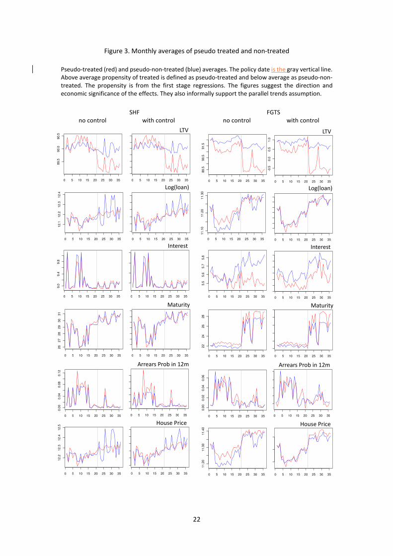
Figure 3 illustrate the effects and visually corroborates the parallel trends assumption

substituting treatment status for an indicator of its likelihood.

The imposition of a maximum LTV limit for new contracts improves the

repayment behavior of treated borrowers, consequently reducing their risk: the

probability of arrears of 15 days or more in the first twelve months of the loan11 decreases

by approximately 9 percentage points (“pp”) and 2 pp in the SFH and the FGTS segment

respectively. Importantly, this result is statistically significant when controlling for tenure

at current employment, economic sector of employment, and other borrower

characteristics that may correlate with job security, and consequently, repayment ability.

Therefore, LTV limits meaningfully reduce the credit risk of treated borrowers, as

expected.

11 Note that we measure credit risk using repayment behavior in the first twelve months of the loan, but it is reasonable to assume that the incentive to default falls sharply due to the constant amortization schedule. Therefore, this information would be enough to make inferences on borrower credit risk.

17

Table 3. Average treatment effect on constrained borrowers, SFH loans only, no controls

LTV>80% LTV>85% LTV>87% LTV>88%

LTV /1 -8.93 -9.65 ** -9.00 *** -8.70 ***

(5.89) (4.42) (3.22) (2.60)

loan (log) -0.25 * -0.50 ** -0.64 *** -0.59 ***

(0.13) (0.20) (0.20) (0.16)

interest rate (p.p.) 0.13 0.61 ** 0.74 *** 0.70 ***

(0.09) (0.25) (0.24) (0.19)

maturity (years) -2.25 ** -3.13 *** -3.34 *** -2.95 ***

(1.06) (0.96) (0.86) (0.76)

prob. arrears first -10.52 -5.14 -3.31 -1.70

12 months (p.p.) (0.09) (0.04) (0.03) (0.02)

house price (log) /2 -0.61 -0.33 ** -0.32 *** -0.23 ***

(0.37) (0.13) (0.10) (0.07)

F (first stage) 1,093 1,104 1,110 1,129

N 168,588 121,812 99,305 86,868

Treated borrowers would have LTV>90% if allowed to do so. The table reports the average treatment

effect on the treated for each variable, as calculated by the two stage estimator by Botosaru and

Gutierrez (2015). The first stage uses pre-regulation data to estimate the propensity score to borrow with

LTV>90%, conditional on house price and borrower income. F statistics refer to the first stage and,

following Botosaru and Gutierrez (2015), show the first stage regression sucessfully discriminate treated

borrowers from the control group. The second stage identifies the effect of the LTV cap using the first-

stage propensities. Standard errors take into account the first stage estimation uncertainty. Columns

show results estimated for borrowers with a minimum LTV increasingly closer to the capped LTV level of

90% for robustness. Minimum LTVs closer to 90% increase the adherence to the paralell trends

assumption implicit in the estimator. Only borrowers that financed homes valued BRL 450,000 or lower

are considered, to avoid confusion between the effects of the LTV cap and a simultaneous increase in

housing price eligibility.

/1 Before the LTV cap, the average LTV for SFH borrowers with LTV>90% is 96.52%. Hence, the effect of

the cap on the average LTV should be around 6.52 p.p. Larger effects than this distance could be

interpreted as evidence that treated borrowers would further increase their LTV if left unconstrained.

/2 The first stage regression for estimating the effect on house prices is conditional only on borrower

income, not on house prices.

18

Table 4. Average treatment effect on constrained borrowers, SFH loans only, with controls

LTV>80% LTV>85% LTV>87% LTV>88%

LTV /1 -11.28 *** -9.35 *** -8.18 *** -7.74 ***

(2.67) (1.49) (0.99) (0.77)

loan (log) -0.43 *** -0.46 *** -0.49 *** -0.42 ***

(0.09) (0.06) (0.05) (0.04)

interest (p.p.) -0.04 0.39 *** 0.45 *** 0.42 ***

(0.04) (0.06) (0.06) (0.04)

maturity (years) -0.30 -1.68 *** -2.20 *** -2.30 ***

(0.58) (0.40) (0.37) (0.34)

prob. arrears first -16.69 *** -11.09 *** -9.34 *** -8.60 ***

12 months (p.p.) (0.05) (0.02) (0.02) (0.01)

house price (log) /2 -0.49 *** -0.34 *** -0.34 *** -0.28 ***

(0.10) (0.05) (0.04) (0.03)

F (first stage) 1,093 1,104 1,110 1,129

N 68,296 48,614 39,517 34,557












housing price eligibility. The sample is restricted to borrowers with formal employment. Controls include

gender, years of education, tenure at current employment, a dummy for public-sector employment,

economic sector, and ZIP code.

/1 Before the LTV cap, the average LTV for SFH borrowers with LTV>90% is 96.52%. Hence, the effect of

the cap on the average LTV should be around 6.52 p.p. Larger effects than this distance could be

interpreted as evidence that treated borrowers would further increase their LTV if left unconstrained.

/2 The first stage regression for estimating the effect on house prices is conditional only on borrower

income, not on house prices.

19

The housing loan contract terms and the house price of the treated borrowers in

the SFH and FGTS segments diverge materially. In both segments, prospective borrowers

that are constrained by the LTV cap must manage a viable alternative to the increased

down payment requirement. Treated borrowers in each segment respond differently and

obtain opposite outcomes in their housing loan contracts, even when controlling for

individual borrower characteristics.

We estimate that the price of homes that are financed by treated SFH borrowers

falls, on average, by 23% to 34% after the LTV regulation. The magnitude of these

changes is economically significant, and suggests that treated SFH borrowers choose

more affordable housing when faced with maximum LTV requirements.

Indeed, we find that the loan amount falls more than the home price itself, which

is coherent with the lower LTVs we find for these treated SFH borrowers. This result

holds for all combinations of individual controls and LTV cutoff levels. The reduction in

LTV that we find for treated SFH borrowers is comparable to the difference between their

average LTV before the regulation and the regulatory maximum of 90%. Therefore, these

borrowers will purchase more affordable housing, but even still, they will only provide a

down payment that accommodates to the minimum required amount.

In spite of these seemingly lower risk characteristics, treated SFH borrowers end

up with less favorable housing loan contracts. The interest rates increase by 0.4 to 0.7 pp

per year, and the contractual maturities are 1.5 to 3 years shorter. A simple simulation

illustrates the economic significance of this result: for a constant loan size, monthly

repayment values increase approximately 2% to 5% due to the higher interest rates and

an additional 1% to 2% because of shorter maturities.

20

Table 5. Average treatment effect on constrained households, FGTS segment, no controls

LTV>80% LTV>85% LTV>87% LTV>88%

LTV /1 -5.75 *** -5.57 *** -5.42 *** -5.40 ***

(0.58) (0.43) (0.38) (0.37)

log_loan -0.45 *** -0.24 *** -0.14 *** -0.09 ***

(0.04) (0.02) (0.02) (0.02)

interest -1.86 *** -1.20 *** -0.89 *** -0.71 ***

(0.20) (0.10) (0.08) (0.07)

maturity -1.49 *** -0.60 -0.41 -0.43

(0.48) (0.50) (0.53) (0.56)

arrears15 -0.02 * -0.01 -0.02 * -0.02 *

(0.01) (0.01) (0.01) (0.01)

log_price /2 0.28 0.16 0.07 0.03

(0.19) (0.11) (0.08) (0.07)

F (first stage) 5,175 4,166 3,421 2,945

N 219,931 136,527 103,401 86,411

/1 The average LTV among LTV>90% minus 90 in SFH segment is -5.48. The effect on LTV should be

around this. Effects higher than this show the statistic in the post regulation would be higher had

regulation not been issued.

/2 The first stage regression for estimating the effect on house prices does not condition on house prices,

only on household income.












housing price eligibility. Although FGTS segment was not required to impose the LTV cap at 90, it was

de facto imposed by banks.

21

Table 6. Average treatment effect on constrained households, FGTS segment, with controls

LTV>80% LTV>85% LTV>87% LTV>88%

LTV /1 -5.01 *** -4.24 *** -4.06 *** -4.01 ***

(0.17) (0.11) (0.10) (0.10)

loan -0.06 *** 0.00 0.02 * 0.02 **

(0.01) (0.01) (0.01) (0.01)

interest -0.75 *** -0.31 *** -0.21 *** -0.13 ***

(0.04) (0.03) (0.03) (0.03)

maturity 1.46 *** 1.93 *** 2.11 *** 2.13 ***

(0.20) (0.18) (0.17) (0.16)

arrears15 -0.04 *** -0.03 *** -0.02 *** -0.02 ***

(0.01) (0.00) (0.00) (0.00)

log_price /3 0.19 *** 0.07 *** 0.01 -0.02

(0.04) (0.02) (0.02) (0.01)

F (first stage) 5,175 4,166 3,421 2,945

N 76,271 47,583 36,202 30,378

/1 The average LTV among LTV>90% minus 90 in SFH segment is -5.48. The effect on LTV should be

around this. Effects higher than this show the statistic in the post regulation would be higher had

regulation not been issued.

/2 The first stage regression for estimating the effect on house prices does not condition on house prices,

only on household income.












housing price eligibility. Although FGTS segment was not required to impose the LTV cap at 90, it was

de facto imposed by banks. The sample is restricted to borrowers with formal employment. Controls

include gender, years of education, tenure at current employment, a dummy for public-sector

employment, economic sector, and ZIP code.

22

Figure 3. Monthly averages of pseudo treated and non-treated

Pseudo-treated (red) and pseudo-non-treated (blue) averages. The policy date is the gray vertical line.

Above average propensity of treated is defined as pseudo-treated and below average as pseudo-non-

treated. The propensity is from the first stage regressions. The figures suggest the direction and

economic significance of the effects. They also informally support the parallel trends assumption.

SHF FGTS

no control with control no control with control

0 5 10 15 20 25 30 35

-2.0

-1.0

0.0

1.0

0 5 10 15 20 25 30 35

-0.6

-0.2

0.2

0.6

0 5 10 15 20 25 30 35

-0.0

50.0

50

.15

0 5 10 15 20 25 30 35

0.0

0.2

0.4

0.6

0 5 10 15 20 25 30 35

-0.0

20.0

20

.06

0 5 10 15 20 25 30 35

-0.0

50.0

50

.15

0 5 10 15 20 25 30 35

12

.112

.21

2.3

12.4

0 5 10 15 20 25 30 35

26

27

28

29

30

31

0 5 10 15 20 25 30 35

89.5

90

.09

0.5

0 5 10 15 20 25 30 35

9.0

9.4

9.8

0 5 10 15 20 25 30 35

0.0

00

.04

0.0

80

.12

0 5 10 15 20 25 30 35

12

.212

.312

.412

.5

0 5 10 15 20 25 30 35

-0.1

00.0

00.1

00.2

0

0 5 10 15 20 25 30 35

-2-1

01

23

0 5 10 15 20 25 30 35

-0.1

0-0

.05

0.0

0

0 5 10 15 20 25 30 35

-0.5

0.0

0.5

1.0

0 5 10 15 20 25 30 35

-0.1

0-0

.06

-0.0

20

.02

0 5 10 15 20 25 30 35

-0.0

10.0

10

.03

0 5 10 15 20 25 30 35

5.5

5.6

5.7

5.8

0 5 10 15 20 25 30 35

22

24

26

28

0 5 10 15 20 25 30 35

11

.20

11

.30

11

.40

0 5 10 15 20 25 30 35

89

.590

.591

.5

0 5 10 15 20 25 30 35

11

.10

11.2

01

1.3

0

0 5 10 15 20 25 30 35

0.0

00.0

20

.04

0.0

6

LTV

Log(loan)

LTV

Log(loan)

InterestInterest

MaturityMaturity

Arrears Prob in 12mArrears Prob in 12m

House PriceHouse Price

23

The fact that these borrowers are taking loans with shorter maturity, even as

interest rates are higher, suggests that lenders push for less favorable contractual terms

for treated SFH borrowers. Note that, for estimation purposes, the untreated borrowers

are those with LTV close enough (from below) to the maximum limit.

Interestingly, housing loan contracts in the FGTS segment, left out of the LTV

regulation but was also constrained in practice, had different outcomes than SFH loans.

The price of financed homes of treated FGTS borrowers is unaffected by the LTV limit.

Compensating for the higher down payment for the same home, both interest rates and

loan maturity become more favorable and produce lower monthly installments, moving

in an opposite direction when compared to loan contracts to treated SFH borrowers.

Several explanations can be found for the difference between outcomes of treated

SFH and FGTS borrowers, such as a different average stock of disposable wealth owned

by FGTS borrowers or other incentives that are observable to banks but not to us.

However, we cannot discard the possibility that the opposite responses are a result of a

strong signal by the macroprudential supervisor about a buildup of systemic vulnerability

in the specific segment targeted by the regulation, the SFH segment.

The middle class, which largely relies on SFH loans to finance their housing,

represented an important source of systemic risk in the U.S. during the 2007 housing

bubble (Adelino, Schoar and Severino (2016)). In Brazil, the BCB is the banking

supervisor and is widely considered to be de facto the main responsible for financial

stability. Hence, it is reasonable to assume that the market interprets a separated

regulation as a sign from the BCB that this specific segment may pose systemic

vulnerabilities in September, 2013.

Two caveats to our results are worth mentioning. The LTV limit that we study

was relatively high (90%) when compared to other caps established in several

24

jurisdictions, ranging from 70% to 80%. The effect could be subject to nonlinear

dynamics, and thus our results would not be directly translatable to other settings. We are

not able to control for prospective borrowers that were driven out of the housing loan

market or postponed home ownership. The pre-regulation average LTV for treated

borrowers were 96.5% and 95.5% for the SFH and FGTS segments, respectively – not far

away from the regulatory limit. Therefore, we could safely argue that a relevant portion

of the treated borrowers indeed adjusted their behavior and their housing loan contract.

6. Conclusion

We show evidence that unexpected LTV limit regulation affects housing loan

contract terms and the subsequent behavior in the subset of borrowers constrained by the

new regulation. Loan repayment behavior improves in both house loan segments

considered in the paper, while loan contract terms other than LTV become less favorable

to the borrower depending on the segment.

In the SFH segments, directly affected by the LTV regulation, the average housing

loan contracts for treated borrowers have higher down payment requirements, higher

interest rates, and shorter maturities. Borrowers apparently compensate these factors by

purchasing more affordable homes. They also make higher down-payments as their LTV

decrease approximately to the new maximum limit. The resulting outcome of all those

shifts is an improved repayment behavior. Treated FGTS borrowers, who are also

constrained to the same LTV limit, settle with housing loan contracts with lower interest

rates and longer maturities, and finance homes at the same price level as before, with an

overall positive effect on repayment behavior.

The comparison between both segments studied in this paper suggests that LTV

regulation is more effective when accompanied by a signal by the macroprudential

25

supervisor of perceived risks in a particular segment. That is, in the segment targeted by

the policy, and only in this segment, loan contract terms become broadly less favorable

and house prices relatively lower. This is consistent with lower credit and house price

growth, albeit in a small segment of the market. It clearly suggests borrowers in the

targeted segment were relatively more constrained by the policy.

The methodology applied in this paper enables the study of policy measures that

are both relevant and widespread: macroprudential policies that constrain the menu of

possible debt contracts. These “asset-side macroprudential policies” (CGFS, 2012)

constitute an important part of the supervisory toolbox to contain the buildup of systemic

risk. The empirical approach suggested in the paper is therefore of broad significance.

26

References

Afanasieff, T, Carvalho, F.L.C.A, De Castro, E, Coelho, R.L, Gregório, J (2015):

“Implementing Loan-to-Value Ratios: The case of auto loans in Brazil (2010-2011)”.

Working Paper No. 380, Central Bank of Brazil, March

Akinci, O., Olmstead-Rumsey, J. (2015) “How Effective Are Macroprudential Policies?

An Empirical Investigation”, International Finance Discussion Papers #1136.

Botosaru, I. Gutierrez, F. (2015) “Difference-in-Differences when the Treatment Status

is Observed in Only One Period”, Victoria University Working Papers, July 7. Available

at http://www.uvic.ca/socialsciences/economics/assets/docs/Botosaur3.pdf

Campbell, John Y., Tarun Ramadorai, and Benjamin Ranish. "The Impact of Regulation

on Mortgage Risk: Evidence from India." American Economic Journal: Economic

Policy 7.4 (2015): 71-102.

Campbell, John Y., and João F. Cocco. "Household Risk Management and Optimal

Mortgage Choice." The Quarterly Journal of Economics (2003): 1449-1494.

Chodorow-Reich, G. (2014): “The Employment Effects of Credit Market Disruptions:

Firm-Level Evidence from the 2008-9 Financial Crisis”. Quarterly Journal of Economics,

v. 129, n.1.

Committee on Global Financial Stability (CGFS) (2012): “Operationalizing the selection

and application of macroprudential instruments”, CGFS Papers No. 48, December

Crowe, C., Dell’ariccia, G., Igan, D., Rabanal, P. (2011): “How to Deal with Real Estate

Booms: Lessons from Country Experiences”, IMF Working Paper #91

Darbar, S., Wu, X. (2015): “Experiences with Macroprudential Policy – Five Case

Studies”. IMF Working Paper #123.

Dell'ariccia, G, Igan, D., Laeven, L, Tong, H., Bakker, B. And Vandenbussche, J. (2012):

“Policies for Macrofinancial Stability: How to Deal with Credit Booms”, IMF Staff

Notes, June.

Drehmann, M., Borio, C., Gambacorta, L., Jiménez, Trucharte, C. (2010):

“Countercyclical capital buffers: exploring options”, BIS Working Papers, n. 317.

Frunke, M., Paetz, M. (2012) “A DSGE-based assessment of nonlinear loan-to-value

policies: Evidence from Hong Kong”, Bank of Finland BOFIT Discussion Papers, 11.

Hallissey, N., Kelley, R., O’malley, T. (2014): “Macro-prudential Tools and Credit Risk

of Property Lending at Irish Banks”, Economic Letter Series, No. 10.

27

Igan, D., Kang, H. D. (2011): “Do Loan-to-Value and Debt-to-Income Limits Work?

Evidence from Korea”, IMF Working Paper #297.

Jácome, L., Mitra, S. (2015): “LTV and DTI Limits-Going Granular”, IMF Working

Paper, WP 15/154.

Lown, C. and Morgan, D. (2006): “The credit cycle and the business cycle: new findings

using loan officer opinion survey”, Journal of Money, Credit and Banking, 38(6), 1575-

97.

Martins, B, and Schechtman, R (2013): “Loan pricing following a Macro Prudential

Within-Sector Capital Measure”, Working Paper n.323, Central Bank of Brazil, August.

Mendoza, E. G. and Terrones, M E (2008): “An anatomy of credit booms: evidence from

macro aggregates and micro data”, IMF Working Paper WP/08/226.

Pereira Da Silva, L.A. and Harris, R.E. (2012): “Sailing through the Global Financial

Storm: Brazil's recent experience with monetary and macroprudential policies to lean

against the financial cycle and deal with systemic risks”. Working Paper No. 290, Central

Bank of Brazil, August.

loan to value policy and housing loans: effects on ... · pdf file1 loan-to-value policy and...

Documents