arX

iv:1

509.

0391

9v2

[qu

ant-

ph]

10

Nov

201

5

Localization in Quantum Walks on a Honeycomb Network

Changyuan Lyu, Luyan Yu, and Shengjun WuKuang Yaming Honors School, Nanjing University, Nanjing, Jiangsu 210023, China

(Dated: October 8, 2018)

We systematically study the localization effect in discrete-time quantum walks on a honeycombnetwork and establish the mathematical framework. We focus on the Grover walk first and rigorouslyderive the limit form of the walker’s state, showing it has a certain probability to be localized atthe starting position. The relationship between localization and the initial coin state is conciselyrepresented by a linear map. We also define and calculate the average probability of localization bygenerating random initial states. Further, coin operators varying with positions are considered andthe sufficient condition for localization is discussed. We also similarly analyze another four-stateGrover walk. Theoretical predictions are all in accord with numerical simulation results. Finally, ourresults are compared with previous works to demonstrate the unusual trapping effect of quantumwalks on a honeycomb network, as well as the advantages of our method.

PACS numbers: 05.40.Fb, 03.67.Lx

I. INTRODUCTION

Quantum walks are generally classified into two cat-egories: discrete-time and continuous-time quantumwalks [1–4]. In this paper we focus on the former whichwere first introduced by Aharonov et al. in 1993. Adiscrete-time quantum walk usually involves a quantumcoin and a walker. The coin controls the walker’s move-ment. Since a quantum coin could be in any super-position state of up and down, quantum walks exhibitmany different features when compared to classical ran-dom walks (see Refs. [5–10]). For example, the quan-tum walker spreads at a rate linear in time in the one-dimensional Hadamard walk [10], much faster than thesquare-root rate in the classical counterpart.

Another uncommon phenomenon in quantum walksis localization. For a classical random walk on a lineor a square network, as well as the one-dimensionalHadamard walk, the probability of finding the walker ata specific position approaches zero when the number ofsteps is large enough [3, 11]. However, Tregenna et al.

numerically discovered that in quantum walks on a 2Dsquare lattice, the walker under the control of Grover’soperator [12] was highly probable to be found at its initialposition, which was called the walker’s localization [13].Inui et al. then rigorously analyzed this phenomenonand owed localization to degenerate eigenvalues of thesystem’s time-evolution operator [14]. Later localizationwas also found in quantum walks on other kinds of lat-tices [11] or with other coin operators [15–18]. Additionaltime-dependent phase gates could also cause localizationin a 2D alternate Hadamard walk according to litera-ture [19].

Some quantum walks have been successfully employedto design effective quantum search algorithms [20–24],whose target is to transform the system to a specific stateat a probability of O(1). Thus the localization effect inquantum walks shows potential applications in designingfast search algorithms. Some simple quantum walk mod-els have already been implemented by experiments [25–

31]. As the structure of graphene, the honeycomb latticehas been paid much attention to recently. It may haveapplication prospects in quantum controlling and com-puting based on 2D hexagonal materials like the grapheneand h-BN [32]. Besides, since the honeycomb lattice ismore complicated than a line or a common 2D squarelattice, we could expect more different characteristics inquantum walks on a honeycomb network.This paper is organized as follows: Sec.II is devoted to

the definition and mathematical framework of quantumwalks on a honeycomb network. In Sec. III, we calculatethe ket in the limit t → ∞ and show the existence oflocalization in the Grover walk, which is in accord withnumerical simulations. Then in Sec. IV, we investigatethe dependence of localization on the initial state andderive a non-zero average localization probability. Quan-tum walks governed by other coin operators are consid-ered and the condition for localization is proposed. Fur-thermore in Sec. V, an extended model with a four-statecoin is analyzed. In Sec. VI, we compare our resultsto previous models and show the different properties ofquantum walks on a honeycomb network.

II. QUANTUM WALKS ON A HONEYCOMB

NETWORK

A. The position space Hp and the coin space Hc

The quantum walk of a particle is usually described bytwo Hilbert spaces, the coin space Hc and the positionspace Hp. Different from an infinite square lattice or anunrestricted line, a honeycomb network is not a kind ofBravais lattice, for here are two types of vertices [33, 34].For example, after we translate the network along the

vector ~E1 in FIG. 1, the new lattice is not identical tothe original one. Besides, orthogonal Cartesian coordi-nates, e.g. X-Y in FIG. 1, are inconvenient for describingthe positions of vertices here. Therefore, we divide thenetwork into rhombuses and set up an oblique coordi-

2

FIG. 1. Honeycomb network. Black and white points are twotypes of vertices. The distance between two nearest verticesis set to 1√

3.

nate system. A vertex is labeled as (x, y, s), where xand y stand for coordinates of the lower left corner of therhombus in which the vertex is contained, and s indicatesthe type of the vertex. We make the convention that ablack (white) vertex is type-0 (type-1), thus any positioneigenket is denoted as |x, y, s〉p, or |~r, s〉p in short, where~r represents (x, y).

On a honeycomb lattice, a particle is able to movein three directions, so the dimension of the coin spaceis three. The eigenstates of the coin are labeled as |1〉,|2〉, and |3〉, corresponding to movement along (against)~E1, ~E2 and ~E3 from a type-0 (type-1) vertex. Whetherthe walker will move along or against these vectors isdetermined by the type of the vertex. The system’s totalstate vector is denoted by a ket in the composite Hilbertspace Hc ⊗Hp.

B. Time-evolution

A single step of quantum walks starts with applyingthe coin operator C on the coin space. We first chooseGrover’s operator G as the coin operator. The three-dimensional form of G reads [12]

G =1

3

−1 2 22 −1 22 2 −1

.

Then, the particle is moved by the conditional shift op-

erator S, expressed as [22]

S =∑

j,s,~r

|j〉〈j| ⊗ |~r − (−1)s~vj , s⊕ 1〉p〈~r, s|, (1)

where

~v1 = (0, 0), ~v2 = (1, 0), ~v3 = (0, 1).

Afterward the next step starts. During a single step,the position type s is changed by the operator S, so theparticle will move in opposite directions in the followingstep. Therefore this is a kind of “flip-flop” shift [35].The time-evolution operator U of the total system is

U = S · (C ⊗ Ip) where Ip is the identity operator actingon the position space. Accordingly the system’s state|Ψt〉 after t steps is derived by applying U on the initialstate for t times:

|Ψt〉 = (U)t|Ψ0〉. (2)

The state vector |Ψt〉 can be expanded in terms of allthe coin and position eigenkets as

|Ψt〉 =∑

j,~r,s

ψjt (~r, s)|j〉 ⊗ |~r, s〉p.

We introduce the vector

|ψt(~r, s)〉 = [ψ1t (~r, s), ψ

2t (~r, s), ψ

3t (~r, s)]

T, (3)

where the superscript T means transpose. The probabil-ity of finding the particle at the position (~r, s) equals thesquared norm of |ψt(~r, s)〉 if its position is measured.Taking into consideration the topology of the honey-

comb network, we can obtain the recursive relations

|ψt+1(~r, s)〉 =3

∑

j=1

Cj |ψt(~r − (−1)s~vj , s⊕ 1)〉 (4)

where Cj is a matrix whose jth row is the same as thejth row of the coin operator C and other elements are allzeros, e.g.

C2 =1

3

0 0 02 −1 20 0 0

.

Applying discrete Fourier transformation (DFT, see Ap-pendix A) to two sides of Eq. (4), we get the recursiverelations in Fourier space:

|ψt+1(k, l, 0)〉 =MC|ψt(k, l, 1)〉, (5a)

|ψt+1(k, l, 1)〉 =M †C|ψt(k, l, 0)〉, (5b)

whereM = Diag1, e−ik, e−il and k and l are wave num-bers corresponding to coordinates x and y.Assume the particle starts from position (0, 0, 0) and

denote the initial state of the coin α|1〉 + β|2〉 + γ|3〉 as[α, β, γ]T. The initial state of the system is therefore

|Ψ0〉 = [α, β, γ]T ⊗ |0, 0, 0〉p, (6)

3

i.e.,

|ψ0(x, y, s)〉 = δs,0δy,0δx,0[α, β, γ]T, ∀x, y ∈ Z.

δa,b is the Kronecker’s delta. After DFT,

|ψ0(k, l, s)〉 = δs,0[α, β, γ]T, ∀k, l ∈ (−π, π]. (7)

According to Eq. (5),

|ψt(k, l, 0)〉 = (MCM †C)t/2|ψ0(k, l, 0)〉 (8)

when t is even. Thus we need to explore the propertiesof the evolution operator U =MCM †C.

III. LIMIT OF THE STATE VECTOR

Since U is unitary, its eigenvalues can be denoted aseiξj . It is not straightforward to show that ξ1 = 0 andξ2 = −ξ3 = θ where θ satisfies

cos θ =1

9[4 cosk + 4 cos l + 4 cos(k − l)− 3]. (9)

Eq. (9) essentially agrees with the results in Refs. [36, 37].The corresponding eigenvectors are

|φj〉 =1

Nj

ei(l−k+ξj) + ei(k−l+ξj) + ei(ξj−k) + ei(ξj−l) − e−ik − e−il + 12e

iξj − 94e

2iξj − 14

−ei(l−k+ξj) + 12e

i(ξj−k) + 12e

−ik − e−il + 12e

iξj + 12

−ei(k−l+ξj) + 12e

i(ξj−l) + 12e

−il − e−ik + 12e

iξj + 12

, (10)

where Nj is a normalization factor.To determine whether the localization will occur, one

needs to calculate P∞(0, 0, 0), i.e., the probability for theparticle to be found at its starting point (0, 0, 0) in thelimit t→ ∞:

P∞(0, 0, 0) = limt→∞

〈ψt(0, 0, 0)|ψt(0, 0, 0)〉. (11)

Obviously, Pt(0, 0, 0) = 0, ∀ odd t. As a result, we onlyneed to pay attention to even-t cases.Substitute the results above into Eq. (8),

|ψt(k, l, 0)〉 =3

∑

j=1

eiξjt/2|φj〉〈φj |ψ0(k, l, 0)〉. (12)

Then the state ket in real space is derived by applyinginverse DFT to Eq. (12),

|ψt(x, y, 0)〉 =1

(2π)2

∫

V2

dkdleikx+ily |ψt(k, l, 0)〉, (13)

specially,

|ψt(0, 0, 0)〉 =1

(2π)2

3∑

j=1

∫

V2

dkdleiξjt/2|φj〉〈φj |ψ0(k, l, 0)〉.

(14)To further simplify the expression of |ψt(0, 0, 0)〉, we

first introduce a mathematical lemma.

Lemma 1. Suppose ϕ(x, y) ∈ L1([a, b] × [c, d]) and it

satisfyies that a.e. x ∈ [a, b], ϕx(y) = ϕ(x, y) is a count-

ably piecewise monotonic function of y, and in each

monotonic interval (cn, dn), ϕx(y) ∈ C2B((cn, dn)) and

the set y | ∂yϕ(x, y) = 0 is countable. Let f(x, y) =g(x, y) + ih(x, y) and g, h ∈ L1([a, b]× [c, d]). Then

limt→∞

∫ b

a

∫ d

c

f(x, y)eiϕ(x,y)t dydx = 0.

The explanations of some notations as well as thedetailed proof are given in Appendix B. Accordingto Lemma 1, we deduce that the contributions to|ψt(0, 0, 0)〉 from items with j = 2, 3 in Eq. (14) arenegligible when t is large enough. This is not hard tounderstand because when t is very large, eiξjt/2 will os-cillate much faster than |φj〉〈φj |ψ0(k, l, 0)〉 as ξj changes.As a result, the integral will become zero when t tendsto infinity and we only need to consider the term withj = 1. Since ξ1 = 0,

|ψ∞(0, 0, 0)〉 ∼ 1

(2π)2

∫

V2

dkdl|φ1〉〈φ1|ψ0(k, l, 0)〉. (15)

In Eq. (15), only |φ1〉 is a function of k, l while

|ψ0(k, l, 0)〉 is constant according to Eq. (7). Conse-quently Eq. (15) could be interpreted as a linear map

from the initial state |ψ0(k, l, 0)〉 to |ψ∞(0, 0, 0)〉. Themap is represented by a transformation matrix F

F =1

(2π)2

∫

V2

dkdl|φ1〉〈φ1|. (16)

The matrix F contains all the information about thewalker’s behavior at its starting point when t→ ∞. Theexistence of localization is directly related to the system’sinitial state via the matrix F . The final form of F is ob-tained by exploiting the results in Eq. (10):

F =1

6

2 −1 −1−1 2 −1−1 −1 2

. (17)

Now we take a numerical example. Assuming [α, β, γ]T =[1, 0, 0]T, which means the initial state of the coin is

4

“moving along ~E1”, the probability of finding the par-ticle at the position (0, 0, 0) after a great number of stepsis |F [1, 0, 0]T|2 = 1/6 accordingly. Apparently, the prob-ability is not zero and the localization is revealed.We also conduct numerical simulations and the results

are illustrated in FIG. 2. A noticeable peak arises inthe left of FIG. 2. The right figure manifests the prob-ability Pt(0, 0, 0) oscillates around our theoretical valueP∞ = 1/6 and clearly exhibits a tendency to converge,indicating the walker does have a nonzero probability tobe localized at its starting point.

IV. CONDITIONS FOR LOCALIZATION

A. Dependence on the initial state

We have seen that the limit behavior of the Groverwalk is represented by Eq. (15). The probabilityP∞(0, 0, 0) is dependent on the coin’s initial state[α, β, γ]T and it may decrease to zero under some cir-cumstances. To verify this point, we work out the eigen-vectors of F :

1√3

111

,1√2

−101

and1√6

−12−1

.

The corresponding eigenvalues are 0, 1/2 and 1/2 respec-tively. So, if the initial coin state is 1√

3[1, 1, 1]T, the uni-

form superposition state of the three eigenstates withoutphase differences, named the Grover state [17], localiza-tion will disappear. Numerical results are illustrated inthe left of FIG. 3 and Pt clearly converges to zero. It alsomanifests the Grover state is the sole initial state caus-ing the walker to be delocalized. This result is consistentwith the conclusion in Ref. [37].On the other hand, the maximal value of P∞(0, 0, 0)

is |1/2|2 = 25%. Any initial coin state which is a linearcombination of 1√

2[−1, 0, 1]T and 1√

6[−1, 2,−1]T will lead

to the maximum. For example, when the initial state[α, β, γ]T = 1√

3[1, ei2π/3, ei4π/3]T, P∞(0, 0, 0) will reach

the maximal probability 25% of localization (FIG. 3).This is totally different from the Grover state above.

B. Average localization probability

Since the probability P∞(0, 0, 0) is dependent on theinitial state of the coin, what is the average probability ifthe initial state is generated randomly? A random purestate of the coin can be obtained by applying a randomunitary operator U3 ∈ SU(3) on an arbitrary coin state,such as |3〉 (see Sec. II A). The average probability isreasonably defined as

P =1

Ω3

∫

P∞;α,β,γdΩ3 =1

Ω3

∫

|FU3|3〉|2dΩ3, (18)

where dΩ3 is the Haar measure of the group SU(3) andΩ3 =

∫

dΩ3, standing for the volume of SU(3). A unitaryoperator U3 is usually expressed with the generators λjof SU(3) and the angular parameters ζj as [38]

U3 = eiλ3ζ1eiλ2ζ2eiλ3ζ3eiλ5ζ4eiλ3ζ5eiλ2ζ6eiλ3ζ7eiλ8ζ8 .

where 0 6 ζ1, ζ5 6 π, 0 6 ζ3, ζ7 6 2π, 0 6 ζ2, ζ4, ζ6 6π2

and 0 6 ζ8 6√3π. Under this representation, the Haar

measure dΩ3 of SU(3) and the random initial state U3|3〉read [39]

dΩ3 = sin 2ζ2 cos ζ4 sin3 ζ4 sin 2ζ6

8∏

j=1

dζj .

U3|3〉 = e−2iζ8/√3

ei(ζ1+ζ3) cos ζ2 sin ζ4−e−i(ζ1−ζ3) sin ζ2 sin ζ4

cos ζ4

. (19)

Thus the average probability is obtained by finishing theintegral in Eq. (18). The result is

P =1

6.

The result manifests that although a Grover state coinwill delocalize the quantum walker, the expected proba-bility P∞ of localization for a random initial state |Ψ0〉 isstill up to 16.7% if we measure the walkers position aftereven-t steps. Thus the localization phenomenon happensvery frequently in our model and it could be useful indesigning some quantum algorithms.

C. Dependence on coin operator

Apart from the initial coin state, it is obvious thatthe crucial point for the localization to occur is the ex-istence of highly degenerate eigenvalue 1 of the operatorU , which is in agreement with literature [11, 14]. Thischaracteristic is undoubtedly determined by Grover’s op-erator G. If there is another coin operator C leading tothe eigenvalue 1 of U , the other two eigenvalues shouldalso be like the form e±iθ where θ is a function of k and l.According to Lemma 1, these two terms in Eq. (14) usu-ally contribute less to the system’s limit behavior, andthe term with eigenvalue 1 may give rise to localization.Then what are the requirements for such a coin operator?We find a sufficient condition.First, we extend the model of quantum walks on a

honeycomb network in Sec.II. In the Grover walk, theoperator C is independent of position. We now releasethis restriction and let the coin operator be related to theposition type. The time-evolution operator becomes

U = S · (C ⊗∑

~r

|~r, 0〉〈~r, 0|+D ⊗∑

~r

|~r, 1〉〈~r, 1|). (20)

Consequently, the evolution operator U in Fourier spaceis modified,

U =MDM †C. (21)

5

FIG. 2. (Color online) Numerical simulation results for the Grover walk on a honeycomb network with the initial stateα = 1, γ = β = 0. The left figure shows the particle’s spatial probability distribution on the honeycomb network after 400steps. Points in the right figure are the probability for finding the walker at its starting point as a function of time t and thehorizontal line is the theoretical result P∞ = 1/6.

FIG. 3. Pmin vs Pmax. In the left figure, localization disappears when the initial state is the Grover state and in the rightfigure P∞(0, 0, 0) reaches the maximal value with the initial coin state 1√

3[1, ei2π/3, ei4π/3]T.

The sufficient condition: If D = C† and the eigen-vectors of C are all real vectors (overall phases are omit-

ted), 1 will be one of U ’s eigenvalues and the localizationis still present.

The proof is given in Appendix C. The Grover walkwe have studied above is a special case since C = G =G† = D. Here we also give another example of the coinoperator

H =1√3

1 1 1

1 ei2

3π ei

4

3π

1 ei4

3π ei

2

3π

. (22)

H looks much more like the three-dimensional versionof Hadamard matrix and H satisfies all the conditionsabove. We take C = H and D = H† with an initial coinstate [1, 0, 0]T and perform numerical simulations. Theresult is given in FIG. 4, which obviously demonstratesthat the walker has a nonzero probability to stay at itsstarting point when t→ ∞.

Specially if we additionally require all the eigenvaluesof C to be ±1, then we will get the sufficient conditionfor localization when the coin operator is independent ofpositions.

V. FOUR-STATE QUANTUM WALKS ON A

HONEYCOMB NETWORK

A. Definition and transformation matrices

In this section, we consider another modified model inwhich the dimension of the coin space is enlarged to four.The additional fourth component represents not hopping,which means the walker is allowed to stay at its currentposition without moving. As a result, the shift operatornow reads

S = |4〉〈4|⊗Ip+3

∑

j=1

∑

s,~r

|j〉〈j| ⊗ |~r − (−1)s~vj , s⊕ 1〉p〈~r, s|,

6

FIG. 4. (Color online) Localization exists when C = H and D = H† with the initial state α = 1 and β = γ = 0.

and the revised recursive relation is given as

|ψt+1(~r, s)〉 = C4|ψt(~r, s)〉+3

∑

j=1

Cj |ψt(~r−(−1)s~vj , s⊕1)〉,

where the coin operator C now should be the four-dimensional Grover’s operator G [12]

G =1

2

−1 1 1 11 −1 1 11 1 −1 11 1 1 −1

. (23)

The fourth coin basis state |4〉 stands for “not moving”.Similarly, the recursive relations in Fourier space Eq. (5)also change to

|ψt+1(k, l, 0)〉 = C4|ψt(k, l, 0)〉+M ′C|ψt(k, l, 1)〉,|ψt+1(k, l, 1)〉 = C4|ψt(k, l, 1)〉+M ′†C|ψt(k, l, 0)〉,

with M ′ = Diag1, e−ik, e−il, 0, which can be furtherexpressed as

[

|ψt+1(k, l, 0)〉|ψt+1(k, l, 1)〉

]

=

[

C4 M ′CM ′†C† C4

] [

|ψt(k, l, 0)〉|ψt(k, l, 1)〉

]

.

Therefore,

[

|ψt(k, l, 0)〉|ψt(k, l, 1)〉

]

= (U ′)t[

|ψ0(k, l, 0)〉|ψ0(k, l, 1)〉

]

, (24)

where U ′ =

[

C4 M ′CM ′C† C4

]

is an 8 × 8 matrix. So we

start to examine the properties of the evolution operatorU ′.The eigenvalues of U ′ are 1, −1, e±iθ1 and e±iθ2 where

θ1 and θ2 are functions of k and l. According to Lemma 1,

when the time t is large enough, we only need to pay at-tention to eigenvalues ±1 and their corresponding eigen-vectors. The eigenvectors are

|φ′1〉 =[eil − eik, 1− eil,−1 + eik, 0, eik − eil,

eik(−1 + eil),−eil(−1 + eik), 0]T

corresponding to 1 and

|φ′2〉 = [−1, 0, 0, 1,−1, 0, 0, 1]T

|φ′3〉 = [0, e−ik, 0,−e−ik, 0, 1, 0,−1]T

|φ′4〉 = [0, 0, e−il,−e−il, 0, 0, 1,−1]T

corresponding to −1.Now, if the walker still starts from the position (0, 0, 0)

with an initial coin state [α, β, γ, µ]T, the initial state ofthe overall system reads

|Ψ0〉 = [α, β, γ, µ]T ⊗ |0, 0, 0〉p

and in Fourier space

|ψ0(k, l, s)〉 = δs,0[α, β, γ, µ]T, ∀k, l ∈ (−π, π].

Since U has two highly degenerate eigenvalues ±1, wedenote

F+ =1

(2π)2

∫

V2

dkdl|φ1〉〈φ1|, (25)

F− =1

(2π)2

4∑

j=2

∫

V2

dkdl|φj〉〈φj |, (26)

where vectors |φj〉 are orthogonalized and normalizedforms of |φ′j〉. Hence, analogous to Eq. (15), for a large twe have

[

|ψt(0, 0, 0)〉|ψt(0, 0, 1)〉

]

∼ (F+ + (−1)tF−)

[

|ψ0(k, l, 0)〉0

]

, (27)

7

or

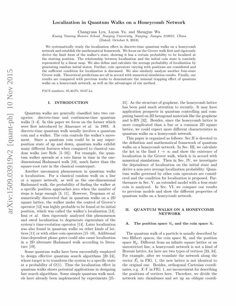
|ψt(0, 0, 0)〉 ∼ (F+ + (−1)tF−)|ψ0(k, l, 0)〉, (28)

where the elements of 4× 4 matrices F± are

(F±)ij = (F±)ij , 1 6 i, j 6 4.

Different from the three-state walk, the extra freedomcauses the probability Pt(0, 0, 0) nonzero when t is odd.However, Eq. (28) implies the transformation matricesfor odd and even t are different, due to the negative eigen-value −1, i.e.

P∞,e(0, 0, 0) = |Fe|ψ0(k, l, 0)〉|2 (29)

P∞,o(0, 0, 0) = |Fo|ψ0(k, l, 0)〉|2 (30)

where Fe = F+ + F− and Fo = F+ − F−. Subscripts ‘e’and ‘o’ stand for ‘even’ and ‘odd’ respectively.On account of the complexity of Eq. (26), we only get

a numerical result of F−:

F− ≈

0.320303 −0.070303 −0.070303 −0.179697−0.070303 0.320303 −0.070303 −0.179697−0.070303 −0.070303 0.320303 −0.179697−0.179697 −0.179697 −0.179697 0.539090

,

while the accurate form of F+ is obtained

F+ =1

12

2 −1 −1 0−1 2 −1 0−1 −1 2 00 0 0 0

. (31)

As an example, with the initial coin state set to1√2[1, 1, 0, 0]T, the value of Pt(0, 0, 0) would converge to

two values

P∞,e = |Fe1√2[1, 1, 0, 0]T|2 ≈ 0.222901 (32)

P∞,o = |Fo1√2[1, 1, 0, 0]T|2 ≈ 0.092699 (33)

according to the derivations above. To confirm the re-sults, numerical simulations are performed, illustrated inFig. (5). The data points do distribute in two branchesand get close to our analytical predictions (the two hori-zontal lines) as the step number t gets large.

B. Maximal, minimal and average probability of

localization

Once we have obtained transformation matrices, theproperties of this quantum walk are easily analyzed. Theeigenvalues of Fe are 0.718787, 0.640606, 0.640606, andzero. Those of Fo are −0.718787, −0.140606, −0.140606and zero, intimating that Po and Pe have equal maximalvalues, about | ± 0.718787|2 ≈ 0.516655, as well as thesame minimum zero. The eigenvectors of Fo and Fe cor-responding to zero are both 1

2 [1, 1, 1, 1]T. So the Grover

FIG. 5. (Color online) Simulation results for four-statequantum walks with initial state 1√

2[1, 1, 0, 0]T (black) and

1

2[1, 1, 1, 1]T (blue).

FIG. 6. When the initial coin state is α = β = γ = −1

2√

3

and µ =√

3

2, the values of Pe and Po converge to the same

limit, about 0.516655.

state is also the sole initial coin state that will delocalizethe particle in four-state walks, which is shown in Fig. 5.What is more interesting is that the eigenvector of Fe

corresponding to 0.718787 is also the same as that ofFo corresponding to −0.718787, whose numerical valuereads

|ϕmax〉 ≈[−0.288675,−0.288675,−0.288675, 0.866025]T

≈ 1

2√3[−1,−1,−1, 3]T.

This suggests if the coin state is initialized with |ϕmax〉,Pe and Po will reach the maximal value simultaneously.The numerical results in Fig. 6 do show that the prob-abilities of localization for even and odd times convergeto a single limit, just as we have calculated. However,the ket |Ψt〉 still oscillates, for Fo|ϕmax〉 is different fromFe|ϕmax〉.The maximum of P∞ here is around twice as much as

that for the previous three-state coin model, indicatingthe localization is much stronger. We consider the aver-age probability again to make a more appropriate com-parison. In this case, arbitrary unitary operators U4 ∈

8

SU(4) and the Haar measure dΩ4 [38] of SU(4) are in-volved:

Pe =1

Ω4

∫

|FeU4|4〉|2dΩ4 ≈ 0.334352, (34)

Po =1

Ω4

∫

|FoU4|4〉|2dΩ4 ≈ 0.139049. (35)

Pe is much larger than P = 1/6 in Sec. IVB and Po

is only slightly smaller than P . In fact the probabilityPt(0, 0, 0) is always zero in the previous model when t isodd. Thus the localization in four-state quantum walksis much stronger than that in the previous model due tothe additional fourth coin state of not hopping.

VI. COMPARISONS WITH PREVIOUS WORKS

Now we compare our results of quantum walks on ahoneycomb network to other kinds of quantum walksstudied in the literature.The first is work [11] by Inui et al about a particle

walking on a line under the control of Grover’s opera-tor. Besides walking left and right, the particle has anadditional freedom to stay at its current position. Sothe coin space is also three-dimensional. For the situa-tion considered by Inui et al, we derive the correspondingtransformation matrix F ′

F ′ =1√6

1√6− 2 2

√6− 5√

6− 2√6− 2

√6− 2

2√6− 5

√6− 2 1

. (36)

Likewise, we calculate the average probability of this walkand get the result P ′ ≈ 0.1684, which is slightly largerthan 1/6 for the three-state Grover walk on a honeycombnetwork. However, we notice that the position space hereis one dimensional but the honeycomb network is a 2Dlattice. Meanwhile, in our case the walker does not havethe extra freedom of “stay”. If the walker on a honey-comb network is also allowed not to hop, just as we cal-culated in Sec. V, the average probability will get muchlarger. Thus we can say the degree of localization is rela-tively high in the Grover walk on a honeycomb network.The particle can be found at its starting position with agood chance.On the other hand, we can find out the maximal value

of P ′∞ in this 1D three-state walk by eigendecomposition

of F ′. The eigenvalues of F ′ are zero,√6− 2 and 3−

√6

and the corresponding eigenvectors are

1√6

1−21

,1√2

−101

and1√3

111

.

Hence the initial coin state 1√6[1,−2, 1]T will delocalize

the walker, which agrees with the result in Ref. [11].

However, the maximum of P ′∞ should be |3 −

√6|2 ≈

0.303 corresponding to the initial coin state 1√3[1, 1, 1]T,

instead of the value 0.202 claimed in Ref. [11]. Actually,one can also get the maximal value 0.303 by submittingα = β = γ = 1/

√3 into Eq. (8) of Ref. [11]. It is obvious

that our mathematical method with the transformationmatrix F is very convenient in studying localization phe-nomena in quantum walks.Apart from the localization probability, another re-

markable difference is that in 1D three-state walks, thelimit state converges to a static wave function, while on ahoneycomb network, the limit ket oscillates between twovalues. Furthermore, the oscillation in four-state walksis not so palpable as that of three-state walks on thehoneycomb network, since it results from the negativeeigenvalue −1 of U ′, the evolution operator in Fourierspace.Kollar et al. in their previous work [40] investigated

another model where the particle walks on a triangularlattice with a three-dimensional coin operator, similarto three-state quantum walks in this paper. The au-thors found when the coin operator is set to Grover’soperator, the walker still has a rapidly decaying prob-ability to be localized at the origin. Analyses suggestthat coin operators leading to localization will transformquantum walks on a 2D plane to quantum walks on aquasi-one-dimensional line. In contrast, Grover walks ona honeycomb network undoubtedly allow the appearanceof localization, and we have also found many more coinoperators leading to walker’s localization in the previ-ous section. Besides, by comparing FIG. 4 with FIG. 2,we can see that walker under the control of H displaysdifferent probability distribution from G. There are non-trivial phenomena present in these models. So we can seequantum walks on a honeycomb network do have moredifferent features.The works [37] by Y. Higuchi et al. and [36] by

Machida also analyzed the localization in quantum walkson a hexagonal lattice. The coin operators are Grover’soperator G and C′, respectively, in their articles, where

C′ =1

2

−1− cos ǫ√2 sin ǫ 1− cos ǫ√

2 sin ǫ 2 cos ǫ√2 sin ǫ

1− cos ǫ√2 sin ǫ −1− cos ǫ

(37)

and the parameter ǫ ∈ [0, 2π). In fact when ǫ is setto arcsin(−1/3), C′ equals Grover’s operator. Their re-sults of long-time limit of the localization probability arecongruent with ours. However, the method of oblique co-ordinate system used to label the vertices in our articleis more intuitive and concise. We have conducted moredetailed analysis such as the average probability and thedependence on the coin operator. Moreover, we can seethat the eigenvectors of C′ are

−101

,

cot ǫ+ csc ǫ

−√2

cot ǫ+ csc ǫ

and

1− cos ǫ√2 sin ǫ

1− cos ǫ

, (38)

and C′ = C′†. So C′ satisfies the sufficient condition inSec. IVC. Thus 1 is one of the the time-evolution oper-ator’s eigenvalue and localization is probable to occur in

9

FIG. 7. (Color online) Relationship between average positionr and time t. Black and blue dots stand for Fig. 2 and Fig. 4,respectively.

Machida’s model according to the more general result inSec. IVC.As a by-product, we numerically estimate the spread-

ing speed of the walker mentioned in their papers. Rea-sonably, we use the average radius r defined as

r =∑

x,y,s

rx,y,sPt(x, y, s) (39)

from the starting point to describe how far the walkerhas reached, where

rx,y,s =

√

3

4(x +

s

3)2 + (y +

x+ s

2)2

is the distance between position (x, y, s) and (0, 0, 0).The results for the circumstances of Fig. 2 and Fig. 4 areplotted in Fig. 7, where the data points are distributedin two lines very well, i.e., the walker is linearly spread-ing on the network and the radius of the ring in Fig. 2and in Fig. 4 are proportional to time, which agrees withRefs. [36] and [37]. Additionally, the difference betweenthe slopes of the two lines indicates the spreading speedis related to the coin operator.

VII. SUMMARY

In this paper, we have established a precise mathemat-ical description of quantum walks on a honeycomb net-work and conducted a comprehensive and rigorous studyon the localization effect. We first set the coin operator toGrover’s operator. With discrete Fourier transformation,we analytically obtained the system’s state vector. Thelocalization probability in the limit of large number ofsteps is connected to the initial coin state through a con-cise transformation matrix F , which completely containsall the information about the walker’s limit behavior. Wethen analytically showed localization and delocalization.The results were all supported by numerical simulations.The average probability of localization’s occurrence is 1/6

if the system’s initial state is randomly generated. Othercoin operators were also discussed and we derived a suf-ficient condition for localization. Further, we extendedthe coin space to four and conducted parallel calcula-tions, finding an oscillating limit state and deriving alarger probability. Some other models in literature werereviewed. Basing on the average probabilities, we con-cluded that the trapping effect of a honeycomb networkis relatively strong. Our mathematical method with thetransformation matrix is very convenient to study local-ization in quantum walks. We numerically showed thewalker’s linear spreading property as well.

ACKNOWLEDGMENTS

We wish to thank Sisi Zhou and Ru Cao for their assis-tance and Yafang Xu, Xingfei Zhou, Hongyi Zhang andProfessor Guojun Jin for their advice. This work is sup-ported by the National Natural Science Foundation ofChina under Grants No. 11275181 and No. 11475084,and the Fundamental Research Funds for the CentralUniversities under Grant No. 20620140531.

Appendix A: discrete Fourier transformation

Suppose X(~m) is a function of ~m, an n-dimensionalvector whose components mj ∈ Z. Its discrete Fouriertransformation is defined as

X(~k) =∑

mj∈Z

X(~m)e−i~k·~m, (A1)

where ~k is an n-dimensional wave vector with componentskj ∈ (−π, π]. The inverse transformation is:

X(~m) =1

(2π)n

∫

Vn

X(~k)ei~k·~md~k. (A2)

The integration region Vn in Eq. (A2) is kj ∈ (−π, π], rep-resenting an n-dimensional hypercube whose sides equal2π in the Fourier space.

Appendix B: Proof for Lemma 1

Mathematical notations are as follows:

• L1([a, b]): the set of Lebesgue integrable real func-tions defined on the interval [a, b].

• C2B(A): the set of bounded real functions defined on

set A with continuous first and second derivatives.

• M([a, b]): the set of Lebesgue measurable real func-tions defined on the interval [a, b].

• P (x), a.e. x ∈ A: the proposition P (x) does nothold only for x ∈ A1 ⊂ A and the Lebesgue mea-sure of A1 is zero.

10

Lemma 2 (Riemann-Lebesgue lemma). If f(x) ∈L1([a, b]), then

limt→∞

∫ b

a

f(x) cos (tx) dx = limt→∞

∫ b

a

f(x) sin (tx) dx = 0.

Lemma 3. If a countably piecewise monotonic func-

tion ϕ(x) definied on [a, b] satisfies that in each mono-

tonic interval (an, bn), ϕ(x) ∈ C2B((an, bn)) and the set

x |ϕ′(x) = 0 is countable, then

limt→∞

∫ b

a

cos (ϕ(x)t) dx = limt→∞

∫ b

a

sin (ϕ(x)t) dx = 0.

(B1)

Proof. We prove it in the case of cosine. The domain of

ϕ(x) can be divided into countable intervals, i.e.,

[a, b) =⋃

n

[an, bb) and [an, bn)∩[am, bm) = ∅, for n 6= m,

and in each interval the function is monotonic. In thiscase, each piece is bounded and differentiable to the sec-ond order.Consider one of those intervals [an, bn). First, based

on the theorem of existence of inverse function, there isan inverse function of ϕ, called ϕ−1. Besides, near theend points an and bn, we have

limǫ→0

∫ a′

n

an

|cos (ϕ(x)t)| dx = limǫ→0

∫ bn

b′n

|cos (ϕ(x)t)| dx = 0,

where a′n = an + ǫ and b′n = bn − ǫ. Because the setx |ϕ′(x) = 0 is countable, ϕ′(a′n) or ϕ

′(b′n) is not zerofor almost all ǫ. Now in the interval [a′n, b

′n), by making

a substitution u = ϕ(x) and integrating by parts, we get

∫ b′n

a′

n

cos (ϕ(x)t) dx =

∫ ϕ(b′n)

ϕ(a′

n)

cos (ut)

ϕ′[ϕ−1(u)]du =

1

t

sin (ut)

ϕ′[ϕ−1(u)]

∣

∣

∣

∣

ϕ(b′n)

ϕ(a′

n)

+1

t

∫ ϕ(b′n)

ϕ(a′

n)

sin (ut)ϕ′′[ϕ−1(u)]

ϕ′[ϕ−1(u)]3 du

=1

t

(

sin (ϕ(b′n)t)

ϕ′(b′n)− sin (ϕ(a′n)t)

ϕ′(a′n)

)

+1

t

∫ ϕ(b′n)

ϕ(a′

n)

sin (ut)ϕ′′ [ϕ−1(u)

]

ϕ′ [ϕ−1(u)]3du. (B2)

Since | sin (ut)| ≤ 1 and ϕ′(a′n) 6= 0, ϕ′(b′n) 6= 0, the firstterm tends zero when t → ∞. For the second term,making inverse substitution again,

∫ ϕ(b′n)

ϕ(a′

n)

ϕ′′ [ϕ−1(u)]

ϕ′ [ϕ−1(u)]3du =

∫ b′n

a′

n

ϕ′′(x)

[ϕ′(x)]2dx

=1

ϕ′(a′n)− 1

ϕ′(b′n).

(B3)

According to Lemma 2, the second term tends to zerowhen t→ ∞.Now Let us see the integral in interval [an, bn)

∫ bn

an

cos (ϕ(x)t) dx = (

∫ a′

n

an

+

∫ b′n

a′

n

+

∫ bn

b′n

) cos (ϕ(x)t) dx.

After letting ǫ→ 0 and t→ ∞,

limt→∞

∫ bn

an

cos (ϕ(x)t) dx = 0.

Finally, since limt→∞

∫ b

a|cos (ϕ(x)t)| dx < b−a is uniformly

convergent, the limit and the sum is commutable. So,

limt→∞

∫ b

a

cos (ϕ(x)t) dx = limt→∞

∑

n

∫ bn

an

cos (ϕ(x)t) dx

=∑

n

limt→∞

∫ bn

an

cos (ϕ(x)t) dx = 0.

Lemma 4. For a countably piecewise monotonic func-

tion ϕ(x) satisfying that in each monotonic interval

(an, bn), ϕ(x) ∈ C2B((an, bn)) and the set x |ϕ′(x) = 0

is countable, if f(x) = g(x) + ih(x) and g, h ∈ L1([a, b]),then

limt→∞

∫ b

a

f(x)eiϕ(x)t dx = 0. (B4)

Proof.

f(x)eiϕ(x)t =g(x) cos (ϕ(x)t) − h(x) sin (ϕ(x)t)

+i[g(x) sin (ϕ(x)t) + ih(x) cos (ϕ(x)t)].

(B5)

For the first term in Eq. (B5), since g ∈ L1([a, b]), ∀ ǫ >0, ∃ a staircase function g1(x) satisfying

∫ b

a

|g(x)− g1(x)| dx < ǫ.

Hence∣

∣

∣

∣

∣

∫ b

a

g(x) cos (ϕ(x)t) dx−∫ b

a

g1(x) cos (ϕ(x)t) dx

∣

∣

∣

∣

∣

≤∫ b

a

|g(x) − g1(x)| dx < ǫ.

11

Because g1 is a staircase function, according to Lemma 3,

limt→∞

∫ b

a

g1(x) cos (ϕ(x)t) dx = 0.

Therefore,

limt→∞

∫ b

a

g(x) cos (ϕ(x)t) dx = 0.

The conclusions are the same for the other three termsin Eq. (B5).

Lemma 5 (Lebesgue’s dominated convergence theorem).Suppose fn(x) ⊂ M([a, b]) and lim

n→∞fn(x) = f(x), a.e.

x ∈ [a, b]. If f(x) is dominated by an integrable function

g(x) in the sense that |f(x)| ≤ g(x), then

limn→∞

∫ b

a

fn(x) dx =

∫ b

a

f(x) dx.

Further, the index can be continuous, namely,

limt→∞

∫ b

a

f(x, t) dx =

∫ b

a

f(x) dx.

Now we prove Lemma 1:

Proof. Set

I(x, t) =

∫ d

c

f(x, y)eiϕ(x,y)t dy.

According to Lemma 4, one can find that

limt→∞

I(x, t) = 0, a.e.x ∈ [a, b].

Besides,

|I(x, t)| =∣

∣

∣

∣

∣

∫ d

c

f(x, y)eiϕ(x,y)t dy

∣

∣

∣

∣

∣

≤∫ d

c

|f(x, y)| dy = G(x),

where G(x) is integrable. According to Lemma 5, we get

limt→∞

∫ b

a

∫ d

c

f(x, y)eiϕ(x,y)t dy dx = limt→∞

∫ b

a

I(x, t) dx = 0.

Appendix C: Proof for the sufficient condition

Denoting the normalized eigenvectors of the matrix Cas |ϕm〉 and corresponding eigenvalues as eiωm (m =1, 2, 3), we can construct a unitary matrix P by ar-ranging three eigenvectors |ϕm〉 together, namely, P =[|ϕ1〉, |ϕ2〉, |ϕ3〉]. Then

PUP † = (PMP †)(PC†P †)(PM †P †)(PCP †)

= (P

1 0 00 e−ik 00 0 e−il

P †)

e−iω1 0 00 e−iω2 00 0 e−iω3

(P

1 0 00 eik 00 0 eil

P †)

eiω1 0 00 eiω2 00 0 eiω3

.

We denote the unitary matrix

(P

1 0 00 e−ik 00 0 e−il

P †)

e−iω1 0 00 e−iω2 00 0 e−iω3

as J . Given that eigenvectors |ϕm〉 are all real vectors,

the matrix P would be a real matrix. Then, PUP † =JJ∗. The determinant of JJ∗ − I is

det(JJ∗ − I) = det(J(J∗ − J†)) = det(J)det(J∗ − J†)

Since the matrix J∗ − J† is an anti-symmetrical three-dimensional matrix, its determinant is zero. Therefore,we have proved that 1 is one of the eigenvalues of thematrix PUP †, as well as the matrix U , because unitarytransformations will not change the eigenvalues of an op-erator.

[1] Y. Aharonov, L. Davidovich, and N. Zagury, Phys. Rev.A 48, 1687 (1993).

[2] D. Meyer, Journal of Statistical Physics 85, 551 (1996).[3] S. Venegas-Andraca, Quantum Information Processing

11, 1015 (2012).[4] F. W. Strauch, Phys. Rev. A 74, 030301 (2006).[5] T. D. Mackay, S. D. Bartlett, L. T. Stephenson, and

B. C. Sanders, Journal of Physics A: Mathematical andGeneral 35, 2745 (2002).

[6] A. Childs, E. Farhi, and S. Gutmann, Quantum Infor-mation Processing 1, 35 (2002).

[7] G. Grimmett, S. Janson, and P. F. Scudo, Phys. Rev. E69, 026119 (2004).

[8] I. Carneiro, M. Loo, X. Xu, M. Girerd, V. Kendon, andP. L. Knight, New Journal of Physics 7, 156 (2005).

[9] H. Schmitz, R. Matjeschk, C. Schneider, J. Glueckert,M. Enderlein, T. Huber, and T. Schaetz, Phys. Rev.Lett. 103, 090504 (2009).

[10] N. Konno, Quantum Information Processing 1, 345(2002).

[11] N. Inui, N. Konno, and E. Segawa, Phys. Rev. E 72,056112 (2005).

[12] L. K. Grover, in Proceedings of the Twenty-eighth Annual

ACM Symposium on Theory of Computing , STOC ’96(ACM, New York, NY, USA, 1996) pp. 212–219.

[13] B. Tregenna, W. Flanagan, R. Maile, and V. Kendon,

12

New Journal of Physics 5, 83 (2003).[14] N. Inui, Y. Konishi, and N. Konno, Phys. Rev. A 69,

052323 (2004).[15] K. Watabe, N. Kobayashi, M. Katori, and N. Konno,

Phys. Rev. A 77, 062331 (2008).[16] M. Stefanak, I. Jex, and T. Kiss, Phys. Rev. Lett. 100,

020501 (2008).[17] M. Stefanak, T. Kiss, and I. Jex, Phys. Rev. A 78,

032306 (2008).[18] B. Kollar, T. Kiss, and I. Jex, Phys. Rev. A 91, 022308

(2015).[19] C. Di Franco and M. Paternostro, Phys. Rev. A 91,

012328 (2015).[20] A. AMBAINIS, International Journal of Quantum Infor-

mation 01, 507 (2003).[21] N. Shenvi, J. Kempe, and K. B. Whaley, Phys. Rev. A

67, 052307 (2003).[22] G. Abal, R. Donangelo, F. l. Marquezino, and R. Por-

tugal, Mathematical. Structures in Comp. Sci. 20, 999(2010).

[23] A. M. Childs and J. Goldstone, Phys. Rev. A 70, 022314(2004).

[24] A. M. Childs, R. Cleve, E. Deotto, E. Farhi, S. Gutmann,and D. A. Spielman, in Proceedings of the Thirty-fifth An-

nual ACM Symposium on Theory of Computing , STOC’03 (ACM, New York, NY, USA, 2003) pp. 59–68.

[25] D. Bouwmeester, I. Marzoli, G. P. Karman, W. Schleich,and J. P. Woerdman, Phys. Rev. A 61, 013410 (1999).

[26] B. C. Travaglione and G. J. Milburn, Phys. Rev. A 65,032310 (2002).

[27] H. B. Perets, Y. Lahini, F. Pozzi, M. Sorel, R. Moran-

dotti, and Y. Silberberg, Phys. Rev. Lett. 100, 170506(2008).

[28] M. Karski, L. Frster, J.-M. Choi, A. Steffen, W. Alt,D. Meschede, and A. Widera, Science 325, 174 (2009).

[29] J. Svozilık, R. d. J. Leon-Montiel, and J. P. Torres, Phys.Rev. A 86, 052327 (2012).

[30] Y.-C. Jeong, C. Di Franco, H.-T. Lim, M. S. Kim, andY.-H. Kim, Nature Communications 4, 2471 (2013).

[31] J. Wang and K. Manouchehri, Physical Implementation

of Quantum Walks (Springer, 2013).[32] A. Pakdel, C. Zhi, Y. Bando, and D. Golberg, Materials

Today 15, 256 (2012).[33] C. Kittel and D. F. Holcomb, American Journal of

Physics 35, 547 (1967).[34] X. Zhai and G. Jin, Journal of Physics: Condensed Mat-

ter 26, 015304 (2014).[35] A. Ambainis, J. Kempe, and A. Rivosh, in Proceedings

of the Sixteenth Annual ACM-SIAM Symposium on Dis-

crete Algorithms, SODA ’05 (Society for Industrial andApplied Mathematics, Philadelphia, PA, USA, 2005) pp.1099–1108.

[36] T. Machida, arXiv.org (2015), quant-ph/1502.06453v1.[37] Y. Higuchi, N. Konno, I. Sato, and E. Segawa, Journal

of Functional Analysis 267, 4197 (2014).[38] T. Tilma and E. C. G. Sudarshan, Journal of Physics A:

Mathematical and General 35, 10467 (2002).[39] M. Byrd, Journal of Mathematical Physics 39, 6125

(1998).[40] B. Kollar, M. Stefanak, T. Kiss, and I. Jex, Phys. Rev.

A 82, 012303 (2010).