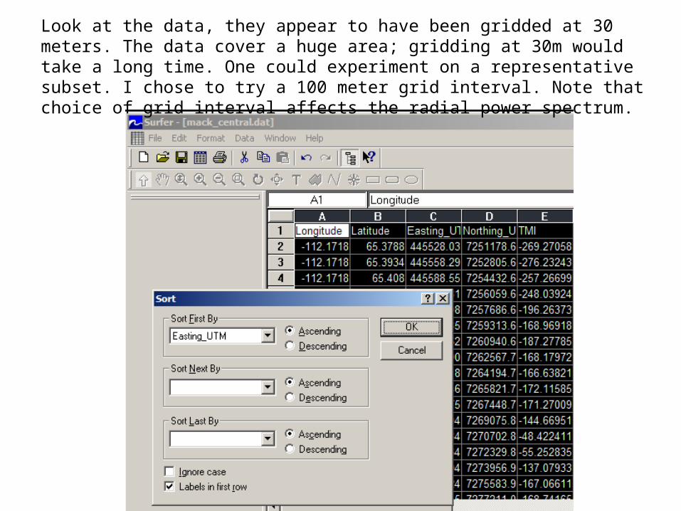
Look at the data, they appear to have been gridded at 30 meters. The data cover a huge area; gridding at 30m would take a long time. One could experiment on a representative subset. I chose to try a 100 meter grid interval. Note that choice of grid interval affects the radial power spectrum.

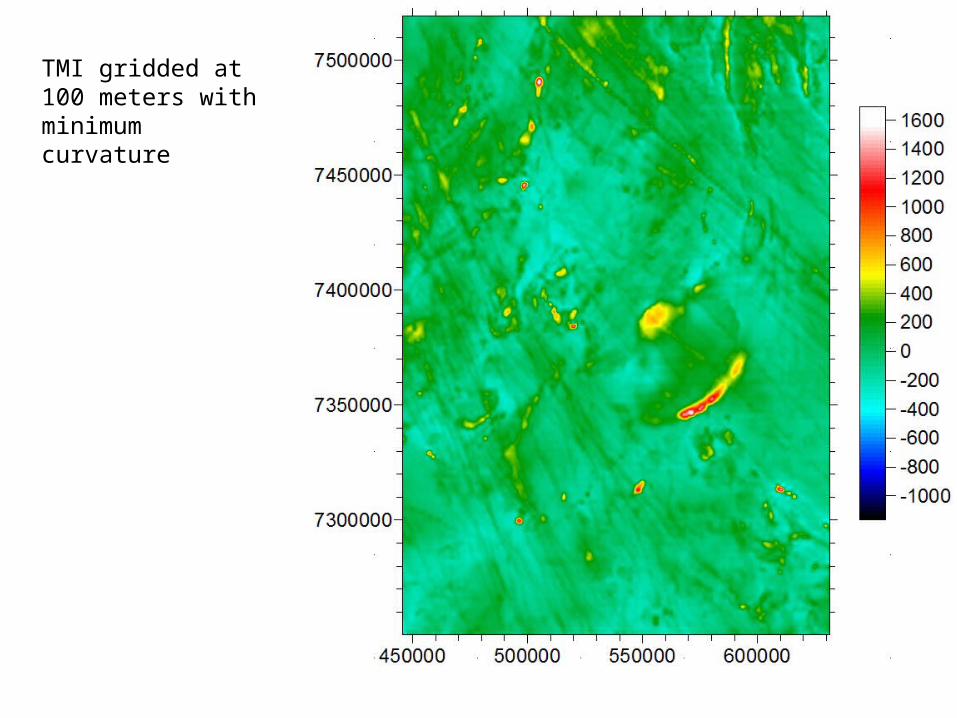
TMI gridded at 100 meters with minimum curvature

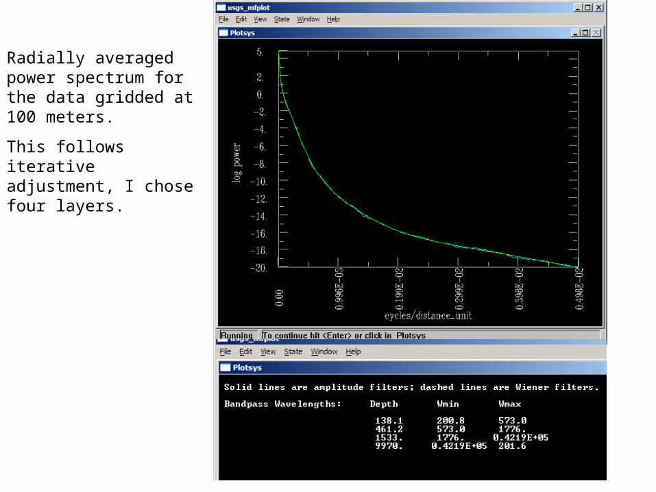
Radially averaged power spectrum for the data gridded at 100 meters.

This follows iterative adjustment, I chose four layers.

Shallowest Dipole Layer

Second deepest equivalent layer

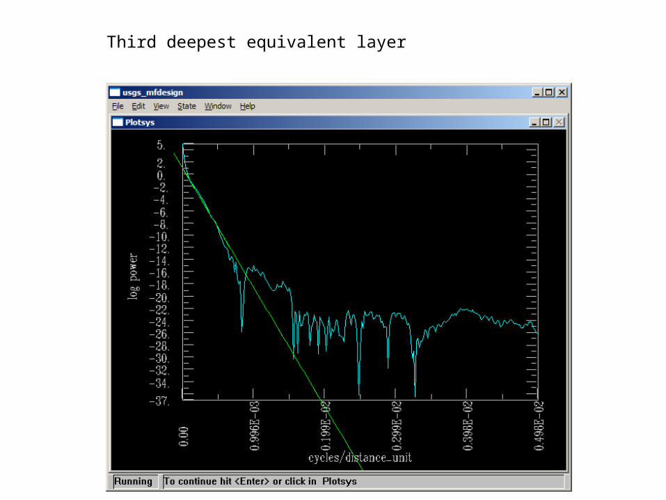
Third deepest equivalent layer

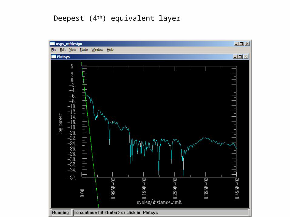
Deepest (4th) equivalent layer

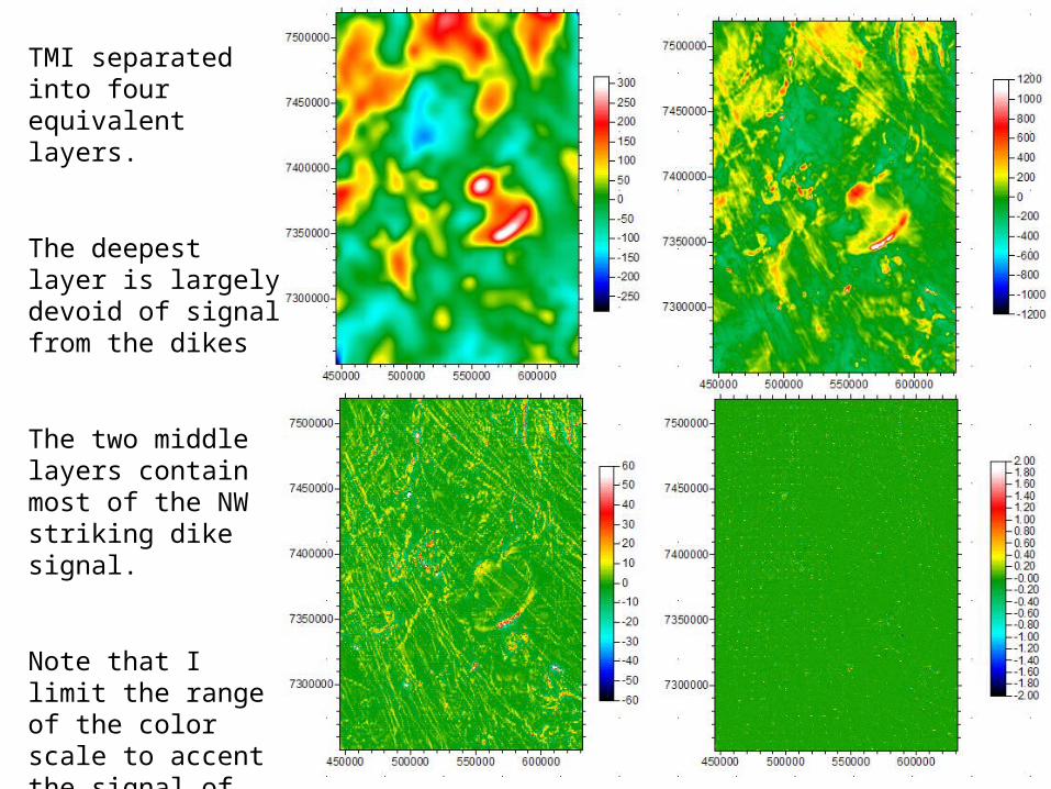
TMI separated into four equivalent layers.

The deepest layer is largely devoid of signal from the dikes

The two middle layers contain most of the NW striking dike signal.

Note that I limit the range of the color scale to accent the signal of interest.

Sum of the middle two equivalent layers (461 meters and 1533 meters) separated by matched filtering.

The dikes are now the dominant signal but there are some interesting anomalies transverse to the dikes

Surfer includes simple (convolution) directional filters – you can use them to bias against directional signal in directional apertures

Application of Simple Directional Filters

Signal with southwest strike removed Subsequent removal of northeast strike

TMI TMI after filtering to separate dikes

450000 500000 550000 600000

7300000

7350000

7400000

7450000

7500000

-400-350-300-250-200-150-100-50050100150200250300350400

Surfer color scheme Geosoft color scheme