low-cost sensors for natural gas …€¦ · 19/3/2013 · gas pipeline monitoring and inspection ....

E n e r g y R e s e a r c h a n d D e v e l o p m e n t D i v i s i o n F I N A L P R O J E C T R E P O R T

LOW-COST SENSORS FOR NATURAL GAS PIPELINE MONITORING AND INSPECTION APPENDICES A - J

DECE MBER 2014 CE C-500-2014-104-AP

Prepared for: California Energy Commission Prepared by: The Regents of the University of California University of California, Berkeley

APPENDICES

APPENDIX A: Benchmarking Existing Diagnostic Approaches for Natural Gas Pipelines .............

APPENDIX B: Micro-Electro-Mechanical Systems Sensor Designs for Natural Gas Pipelines ........

APPENDIX C: Workshop Notice ...............................................................................................................

APPENDIX D: Workshop Notes ................................................................................................................

APPENDIX E: Laboratory Testing of Low-Cost Sensors for Natural Gas Pipelines ..........................

APPENDIX F: Sensors Test Bed Design and Validation ........................................................................

APPENDIX G: Sensor Testing in the Test Bed .........................................................................................

APPENDIX H: Data Analysis of Sensor Testing .....................................................................................

APPENDIX I: Miniaturization and Lifetime Testing of Sensors ...........................................................

APPENDIX J: Workshop .............................................................................................................................

APPENDIX A: Benchmarking Existing Diagnostic Approaches for Natural Gas Pipelines

A-1

Prepared by: University of California, Berkeley Primary Author(s): Sean Wihera Igor Paprotny Yipping Zhu Richard M. White Paul K. Wright Gaymond Yee Contract Number: 500-10-044 Prepared for: California Energy Commission Johann Karkheck Contract Manager Johann Karkheck Project Manager Fernando Pina Office Manager Energy Systems Research Office Laurie ten Hope Deputy Director Energy Research & Development Division

Robert P. Oglesby Executive Director

DISCLAIMER

This report was prepared as the result of work sponsored by the California Energy Commission. It does not necessarily represent the views of the Energy Commission, its employees or the State of California. The Energy Commission, the State of California, its employees, contractors and subcontractors make no warrant, express or implied, and assume no legal liability for the information in this report; nor does any party represent that the uses of this information will not infringe upon privately owned rights. This report has not been approved or disapproved by the California Energy Commission nor has the California Energy Commission passed upon the accuracy or adequacy of the information in this report.

ACKNOWLEDGEMENTS

We would like to thank our Project Advisory Committee for their support and guidance on this project. We would also like to thank Fernando Pina, Jamie Patterson and Mike Gravely for stimulating discussion and guidance.

A-3

PREFACE

The California Energy Commission Public Interest Energy Research (PIER) Program supports public interest energy research and development that will help improve the quality of life in California by bringing environmentally safe, affordable, and reliable energy services and products to the marketplace.

The PIER Program conducts public interest research, development, and demonstration (RD&D) projects to benefit California.

The PIER Program strives to conduct the most promising public interest energy research by partnering with RD&D entities, including individuals, businesses, utilities, and public or private research institutions.

PIER funding efforts are focused on the following RD&D program areas:

• Buildings End-Use Energy Efficiency

• Energy Innovations Small Grants

• Energy-Related Environmental Research

• Energy Systems Integration

• Environmentally Preferred Advanced Generation

• Industrial/Agricultural/Water End-Use Energy Efficiency

• Renewable Energy Technologies

• Transportation

Benchmarking Existing Diagnostic Approaches for Natural Gas Pipelines is the interim report for the Natural Gas Pipeline Sensor project (contract number 500-10-044), conducted by University of California, Berkeley. The information from this project contributes to PIER’s Energy Systems Integration Program.

For more information about the PIER Program, please visit the Energy Commission’s website at www.energy.ca.gov/research/ or contact the Energy Commission at 916-654-4878.

A-4

http://www.energy.ca.gov/research/

ABSTRACT

This report provides a series of qualitative benchmarks upon which existing natural gas pipeline diagnostic technologies are evaluated. The authors of this report worked in conjunction with the California investor-owned utilities companies Pacific Gas and Electric (PG&E), San Diego Gas and Electric (SDG&E), and Southern California Gas (SoCalGas) to develop these basic metrics for the qualitative comparison of existing diagnostic tools and those under development at the Center for Information Technology Research in the Interest of Society (CITRIS) at the University of California Berkeley. Existing technologies are evaluated on three parameters: disruption of service, reporting frequency and the price and size of the diagnostic technology. The authors have found that much of the existing diagnostic technologies are large, expensive, or require a cessation in pipeline activity to be implemented.

Keywords: Natural Gas Pipeline Diagnostics, Benchmark.

Please use the following citation for this report:

Sean Wihera, Paprotny, Igor, Yiping Zhu, Richard M. White, Paul K. Wright, Gaymond Yee. (University of California, Berkeley). 2012 Benchmarking Existing Diagnostic Approaches for Natural Gas Pipelines. California Energy Commission. Publication number: CEC-XXX-2012-XXX.

A-5

TABLE OF CONTENTS

Acknowledgements .................................................................................................................................. 3

PREFACE .................................................................................................................................................... 4

ABSTRACT ................................................................................................................................................ 5

TABLE OF CONTENTS ........................................................................................................................... 6

CHAPTER 1: Introduction ....................................................................................................................... 7

1.1 Benchmarking Parameters........................................................................................................... 7

CHAPTER 2: Existing Diagnostic Techniques .................................................................................... 9

2.1 Hydrostatic Testing ...................................................................................................................... 9

2.2 Pigs .................................................................................................................................................. 9

2.3 Common Pipe Wall Diagnostic Techniques ........................................................................... 10

2.3.1 Magnetic Flux Leakage ....................................................................................................... 10

2.3.2 Eddy Current Testing .......................................................................................................... 11

2.3.3 Ultrasonic Testing ................................................................................................................ 12

2.3.4 Electromagnetic Acoustic Transducer .............................................................................. 13

2.4 Existing Benchmarking Sensors ................................................................................................ 14

2.4.1 Vibration ............................................................................................................................... 14

2.4.2 Flow ....................................................................................................................................... 14

2.4.3 Moisture ................................................................................................................................ 15

2.4.4 Odorant ................................................................................................................................. 16

CHAPTER 3: Conclusion ....................................................................................................................... 19

References................................................................................................................................................. 20

A-6

CHAPTER 1: Introduction This report serves as a comparison of common existing natural gas sensor solutions to the micro-electro-mechanical systems (MEMS)-based sensor solutions currently being developed by the Center for Information Technology in the Interest of Society (CITRIS) at the University of California Berkeley. In addition to common pipeline diagnostic techniques, the researchers also benchmark existing off-the-shelf sensing technologies, specifically focusing on vibration, flow, moisture, odorant sensors.

The diagnostic technologies analyzed in this paper are qualified in terms of the following three parameters:

1. Does the diagnostic require a disruption of service or temporarily take the pipeline offline?

2. Does the diagnostic report/transmit data continuously or intermittently? 3. What is the general size of the diagnostic technology? What is the general cost?

The research team has also engaged with three investor-owned utilities in California (Pacific Gas and Electric (PG&E), San Diego Gas and Electric (SDG&E), and Southern California Gas (SoCalGas)) to develop these basic metrics for the qualitative comparison of existing diagnostic tools and those under development at the CITRIS. The goal was to identify pertinent existing diagnostic technologies for benchmarking purposes and future comparisons with the sensor suite currently being designed.

1.1 Benchmarking Parameters 1.1.1 Disruption of Service (Online/Offline) The first of the three parameters upon which existing diagnostic technologies are benchmarked is disruption of service. When inspecting a gas line, varying diagnostic technologies either require or do not require a cessation in gas transmission. Taking part of the pipeline offline during an inspection can be both costly and potentially result in a disruption of service to ratepayers. Consequently, diagnostic techniques which safely operate while the lines are in service are desirable.

1.1.2 Frequency of Data Reporting (Continuous/Intermittent) The second parameter upon which existing diagnostic technologies are benchmarked is reporting frequency. Diagnostic techniques either report information intermittently or continuously. Many traditional diagnostic techniques, particularly those requiring a disruption of service, provide only periodic diagnostics when inspections are actively made by utility employees. Inversely, continuous condition-based monitoring diagnostic techniques can report on potentially hazardous changes in real-time. Such continuous reporting is viewed as highly desirable due to both proactive and reactive advantages.

A-7

1.1.3 Cost The third parameter upon which existing diagnostic techniques shall be evaluated is cost. Lower costs enable utilities to implement these diagnostics more widely throughout the transmission network. Not all price information was readily available. Some of the prices had to be estimated based on prices of similar type/size sensors, as well as on interviews with the utilities.

1.1.4 Size Reduced package size eases the implementation of such diagnostic technologies. Additionally, the size of the diagnostic technology packaging is often a determinant of whether a specific diagnostic can be performed while a line is in service.

A-8

CHAPTER 2: Existing Diagnostic Techniques 2.1 Hydrostatic Testing Hydrostatic testing is the definitive pressure diagnostic for gas pipelines. The diagnostic involves temporarily disconnecting a section of pipeline and pressurizing it with water. The water pressure is increased to 125% of the maximum operating pressure (MAOP) where it is held for eight hours. Hydrostatic testing is recognized as a “destructive” diagnostic as the failure of a pressurized pipe results in a rupture and the consequent destruction of the pipe. Should a pipeline fail a hydrostatic test, the only option is to replace the destroyed section of pipeline. Understandably, the replacement of pipeline comes at a large cost to the utility company. Consequently, there is a large interest in the development of nondestructive diagnostics.

Characteristics: • Requires pipeline be offline • Failure results in destruction of pipeline section • Expensive • Labor intensive • Definitive detection results

Figure 1: Hydrostatic pressure testing diagram

Source: Pacific Gas & Electric (PG&E, 2012)

2.2 Pigs Pigs, devices that travel through the pipeline (initially named by the characteristic pig-like squealing as one moved through the pipe), are the industry’s nondestructive standard for in-line inspections. Pigs provide a mobile platform upon which a variety of sensors and equipment can be mounted for varying diagnostics throughout the line. The use of pigs requires the

A-9

targeted line be taken out of service and all gas vented from the inspection zone. Additionally, inserting pigs into the lines is a highly costly and labor-intensive endeavor. The cost of running a pig is estimated at roughly $1 million fixed cost, and $125,000 per mile of pipeline. As a result, sections of pipe are inspected with a pig very intermittently.

Of the various sensor arrays mounted on pigs, magnetic flux leakage and electromagnetic acoustic transduction packages are used for detecting corrosion and other physical abnormalities. Additionally, video recording and cleaning equipment can be mounted on PIGs for additional visual inspections and maintenance.

Characteristics: • Requires pipeline be offline • Intermittent Reporting • Expensive, large platform • Labor intensive

Figure 2: Example of a Magnetic Flux Leakage pig

Photo Credit: Sandia National Laboratories (Bickerstaff, Vaughn and Stoker, no date)

2.3 Common Pipe Wall Diagnostic Techniques 2.3.1 Magnetic Flux Leakage Magnetic Flux Leakage (MFL) detection is a nondestructive technique used to detect pipeline abnormalities. MFL is typically used in conjunction with the aforementioned pig. The process involves applying a magnetic field to the desired wall of the pipeline and observing anomalies within the magnetic fields resulting from defects within the pipe wall.

Characteristics: • Diagnostic typically used in conjunction with pig requiring pipeline be offline • Provides intermittent pipeline data • Inexpensive (when cost is separated from pig requirement)

A-10

Figure 3: Magnetic Flux Leakage diagram

Source: Gas Technology Institute (Teitsma, A, 2004)

2.3.2 Eddy Current Testing Eddy current Testing (ET) detection is a non-destructive electromagnetic technique used for crack and laminar defect detection. The ET diagnostic detects defects through impedance anomalies when an energized coil is applied either internally or externally. As ET detection can be applied externally, it is not necessary to have the pipeline offline. ET inspection is considered intermittent as it requires an operator to manually move, locate and analyze specific regions of the pipeline. Thus, no region of the pipeline is under continuous inspection.

Characteristics: • Diagnostic does not inhibit pipeline operation • Intermittent Reporting • Inexpensive • Requires operator

Defect Pipe Wall Section

A-11

Figure 4: Eddy current detection diagram

Source: Olympus Technologies (2012)

2.3.3 Ultrasonic Testing Ultrasonic Testing (UT) has been implemented for external diagnostics. This diagnostic relies on the use of ultrasonic transducers to measure pipe wall thickness and detect cracks. This nondestructive process is accurate, yet particularly expensive. And similarly to ET inspection requires an operator to manually move, locate and analyze specific regions of the pipeline resulting in non-continuous reporting.

Characteristics: • Diagnostic does not inhibit pipeline operation • Intermittent Reporting • Expensive • Requires operator

A-12

Figure 5: Technician using Ultrasonic Testing on pipe

Photo Credit: Olympus Technologies (2012)

2.3.4 Electromagnetic Acoustic Transducer Electromagnetic Acoustic Transducer (EMAT) is a newer method of ultrasonic testing. EMAT is used in conjunction with a pig and is a noncontact, nondestructive diagnostic for measuring pipe wall thickness (circumferentially) and identifying pipe wall abnormalities.

Characteristics: • Used in conjunction with PIG, inhibits pipeline operation • Intermittent reporting

Figure 6: Electromagnetic Acoustic Transducer diagram

Source: Oak Ridge National Laboratory (Varma, 2002)

A-13

2.4 Existing Benchmarking Sensors There are a variety of off-the-shelf function-specific diagnostic sensors that may be potentially used by the utilities to address specific sensing requirements throughout the pipeline. The following products have been organized by their specific sensory function.

2.4.1 Vibration Vibration detection can be used to identifying catastrophic events (such as an impact to the pipeline) or other anomalies that would endanger the integrity of the pipeline. Additionally, through continuous monitoring of vibration signatures potential pipeline failures may be identified and proactively addressed.

Analog Devices ADXL337 is an inexpensive, tri-axial accelerometer. Its tiny 3x3x1.5 millimeter (mm) package and low cost ($1.57 per unit for 1000 units) make it a particularly desirable for large-scale dispersion throughout/along the pipeline (Analog Devices, 2012).

Characteristics: • Does not inhibit pipeline operation • Continuously reporting • Very inexpensive/very small package

2.4.2 Flow Flow monitoring can be used to detect leaks or obstructions within the pipeline that could result in either reduction of service or a hazardous situation such as the over pressurization of the pipeline.

Honeywell VersaFlow is a line of industrial flow meters. Honeywell’s selection of gas flow meters includes those operating on coriolis, vortex and magnetic principles (Honeywell, 2012).

Characteristics: • Large/Expensive • Continuous reporting • Does not interfere with pipeline operation

Siemens SITRANS is a line of industrial flow meters. Siemen’s selection of gas flow meters includes those operating on coriolis, vortex and magnetic principles (Siemens, 2012).

Characteristics: • Large/Expensive • Continuous Reporting • Does not interfere with pipeline operation

A-14

2.4.3 Moisture Moisture can occur within natural gas pipelines due to changes in temperature, gas composition, flow rate and position of the pipeline. As moisture can ultimately result in corrosion within the pipeline it is advantageous to proactively monitor the existing moisture content of the natural gas.

MEMS Vision MV2001 is a low power MEMS-based moisture sensor chip. The MV2001 can be integrated to provide high accuracy, high-speed humidity data.

Characteristics: • Small/inexpensive • Continuous reporting • Does not inhibit pipeline operation

Figure 7: MEMS Vision MV2001 moisture sensor

Photo Credit: MEMS Vision (2012)

General Electric (GE) PM880 and M Series Moisture Probe is an aluminum oxide-based moisture sensor that works in conjunction with GE’s portable hygrometers (such as the PM880). The hygrometer includes data logging and transmission capabilities for analysis on a computer.

Characteristics: • Expensive • Continuous reporting • Typically manual operation • Does not inhibit pipeline operation

A-15

Figure 8: General Electric PM880 portable hygrometer; Figure 9: General Electric M Series moisture probe

Photo Credit: General Electric (2012a) Photo Credit: General Electric (2012b)

2.4.4 Odorant Federal law requires that natural gas, which is naturally odorless, be given an odor for detective safety reasons. Natural gas is both flammable and capable of causing asphyxiation. By odorizing natural gas, individuals are able to smell leaks thus preventing potential explosions and reducing the risk of unknowingly entering an asphyxiating environment. As a result various chemical mercaptans (such as methyl mercaptan, tertiary butyl mercaptan) are added to the gas prior to transmission.

Draeger Pac III is a personal gas monitor. This sensor can be fitted to detect the level of mercaptan (or other gases) within the ambient air. The Pac III is designed for use by a fulltime operator and costs several hundred dollars.

Characteristics: • Does not inhibit pipeline operation • Continuously reporting • Operator reliant • Expensive/Non-MEMS package

A-16

Figure 10: Draeger PAC III personal gas monitor

Photo Credit: BSRIA Instrument Solutions (2012)

Detcon DM-700-CH3SH is an industrial toxic gas detection sensor. The Detcon DM-700 is designed to be attached to the pipeline via an access point from which the device can monitor the levels of odorant (methyl mercaptan). The total package is 280x 155 x 96mm which includes a junction box. Proper use of the DM-700 through an appropriate access point would not interfere with transmission of gas within the pipeline.

Characteristics: • Does not inhibit pipeline operation • Continuously reporting • Expensive/Non-MEMS package

A-17

Figure 11: Detcon DM-700 toxic gas detection monitor

Photo Credit: Detcon (2012)

A-18

CHAPTER 3: Conclusion The benchmark study was performed keeping in mind that low-cost MEMS-based sensors can potentially be alternative technologies and that such MEMS-based sensors can be fabricated in the Marvel Nanofabrication facility on the UC Berkeley campus. With in-house fabricated MEMS sensors in mind, the benchmark study was conducted using the following attributes:

• Disruption of service (Offline versus online operation) • Frequency of Reporting (continuous versus intermittent) • Cost • Size

The most common diagnostic techniques were intermittent, or require offline operation. Furthermore, most off-the-shelf sensors were expensive, preventing ubiquitous deployment. Two types of of-the-shelf sensor concepts that stood out for deployment on a MEMS sensor module were the vibration sensor, based on a 3-axis MEMS accelerometer, and MEMS flow sensors. However, it is unclear whether the MEMS flow sensor allows easy integration into the envisioned MEMS sensor module.

A-19

References Analog Devices. (2012). MEMS Inertial Sensors, ADXL337 <http://www.analog.com/en/mems-

sensors/mems-inertial-sensors/adxl337/products/product.html>

Bickerstaff, M. Vaughn, and G. Stoker. (Year unavailable - Post 2002) “Review of Sensor Technologies for In-line Inspection of Natural Gas Pipelines,” <http://www.netl.doe.gov/technologies/oil-gas/publications/Status_Assessments/71702.pdf>

BSIRA. (2012). Instrument Solutions, < http://www.bis.fm/products/Drager_Pac_III.asp>

Detcon Inc. (2012). Toxic Gas Detection Sensors, DM-700, < http://www.detcon.com/1-documents/data_sheets/1-sensors/Model%20700/DM-700/Methyl%20Mercaptan%20DM-700-CH3SH%20PDS.pdf>

General Electric. (2012a). Portable Hygrometers, PM880 < http://www.ge-mcs.com/en/moisture-and-humidity/portable-hygrometers/pm880-portable-hygrometer.html>

General Electric. (2012b). Moisture Probes, M-Series Aluminum Oxide Moisture Probe < http://www.ge-mcs.com/en/moisture-and-humidity/moisture-probes/m-series.html>

Honeywell. (2012). Flow Measurement, <http://hpsweb.honeywell.com/Cultures/en-US/Products/Instrumentation/flow/default.htm>

MEMS Vision. (2012). MV2001, http://www.mems-vision.com/humiditysensors.html

Olympus Technologies. (2012). <http://www.olympus-ims.com/en/intro/>

Pacific Gas & Electric (PG&E). (2012) <http://www.pge.com/myhome/edusafety/systemworks/gas/pipelinesafety/hydrostatictesting/index.shtml>

Siemens. (2012). Flow Measurement, <www.automation.siemens.com/w1/automation-technology-flow-measurement-18626.htm>

Teitsma, A. (2004). “Technology Assessment for Delivery Reliability for Natural Gas – Inspection Technologies: REFC,” <http://www.netl.doe.gov/technologies/oil-gas/publications/Status_Assessments/42266-041201Technology%20Assesment%20Reliability.pdf>

Varma, V.K., [2002]“State of the Art Natural Gas Pipe Inspection” U. S. Department of Energy Report, National Energy Technology Center, pp. 1-5, 2002, Sept 16-17, Natural Gas Infrastructure Reliability Industry Forum, NETL, Morgantown WV. <http://www.netl.doe.gov/technologies/oil-gas/publications/status_assessments/5_pager_1.pdf>

A-20

http://www.analog.com/en/mems-sensors/mems-inertial-sensors/adxl337/products/product.html

http://www.analog.com/en/mems-sensors/mems-inertial-sensors/adxl337/products/product.html

http://www.netl.doe.gov/technologies/oil-gas/publications/Status_Assessments/71702.pdf

http://www.netl.doe.gov/technologies/oil-gas/publications/Status_Assessments/71702.pdf

http://www.bis.fm/products/Drager_Pac_III.asp

http://www.detcon.com/1-documents/data_sheets/1-sensors/Model%20700/DM-700/Methyl%20Mercaptan%20DM-700-CH3SH%20PDS.pdf



http://www.ge-mcs.com/en/moisture-and-humidity/portable-hygrometers/pm880-portable-hygrometer.html

http://www.ge-mcs.com/en/moisture-and-humidity/portable-hygrometers/pm880-portable-hygrometer.html

http://www.ge-mcs.com/en/moisture-and-humidity/moisture-probes/m-series.html

http://hpsweb.honeywell.com/Cultures/en-US/Products/Instrumentation/flow/default.htm

http://hpsweb.honeywell.com/Cultures/en-US/Products/Instrumentation/flow/default.htm

http://www.mems-vision.com/humiditysensors.html

http://www.olympus-ims.com/en/intro/

http://www.pge.com/myhome/edusafety/systemworks/gas/pipelinesafety/hydrostatictesting/index.shtml

http://www.pge.com/myhome/edusafety/systemworks/gas/pipelinesafety/hydrostatictesting/index.shtml

http://www.automation.siemens.com/w1/automation-technology-flow-measurement-18626.htm

http://www.automation.siemens.com/w1/automation-technology-flow-measurement-18626.htm

http://www.netl.doe.gov/technologies/oil-gas/publications/Status_Assessments/42266-041201Technology%20Assesment%20Reliability.pdf

http://www.netl.doe.gov/technologies/oil-gas/publications/Status_Assessments/42266-041201Technology%20Assesment%20Reliability.pdf

http://www.netl.doe.gov/technologies/oil-gas/publications/status_assessments/5_pager_1.pdf

APPENDIX B: Micro-Electro-Mechanical Systems Sensor Designs for Natural Gas Pipelines

B-1

Prepared by: University of California, Berkeley Primary Author(s): Igor Paprotny Yipping Zhu Sean Wihera Richard M. White Paul K. Wright Gaymond Yee Contract Number: 500-10-044 Prepared for: California Energy Commission Johann Karkheck Contract Manager Johann Karkheck Project Manager Fernando Pina Office Manager Energy Systems Research Office Laurie ten Hope Deputy Director Energy Research & Development Division


DISCLAIMER


B-2

ACKNOWLEDGEMENTS

We would like to thank our Project Advisory Committee for their support and guidance on this project. We would also like to thank Fernando Pina, Jamie Patterson and Mike Gravely for stimulating discussion and guidance.

This report was written based on contributions from several authors. Chapters 1, 2 and 5 were written by Igor Paprotny, Chapter 3 was written by Igor Paprotny and Yiping Zhu, while Chapter 4 was written by Richard White. The report was edited by Igor Paprotny and Gaymond Yee.

B-3

PREFACE












• Transportation

Micro-Electro-Mechanical System Sensors Designs for Natural Gas Pipelines is the interim report for the Natural Gas Pipeline Sensors project (contract number 500-10-044), conducted by University of California, Berkeley. The information from this project contributes to PIER’s PIER’s Energy Systems Integration Program.


B-4


ABSTRACT

This report presents the preliminary designs for micro-electro-mechanical system (MEMS) natural gas sensors. This report describes the system wide designs, which include the architecture that will be used to install the inline sensors, as well as the MEMS solutions that are being developed. After conducting a needs-assessment analysis, the research team focused this project on four types of sensors: low-cost and low power MEMS pressure sensors, MEMS flow sensors, and MEMS accelerometers (implementing off-the-shelf solutions). This report also describes preliminary design ideas for Laser Ultrasonic Testing setup.

Keywords: Natural Gas Pipeline Diagnostics, MEMS Sensors, Pressure, Flow, Acceleration, Laser ultrasonic Testing.


Paprotny, Igor, Yiping Zhu, Sean Wihera, Richard M. White, Paul K. Wright, Gaymond Yee. (University of California, Berkeley). 2012. Micro-Electro-Mechanical System Sensor Designs for Natural Gas Pipelines. California Energy Commission. Publication number: CEC-XXX-2012-XXX.

B-5

TABLE OF CONTENTS


PREFACE .................................................................................................................................................... 4

ABSTRACT ................................................................................................................................................ 5


CHAPTER 1: Introduction ....................................................................................................................... 8

Report Structure ..................................................................................................................................... 8

CHAPTER 2: System Level Design ........................................................................................................ 9

CHAPTER 3: Sensor Designs ................................................................................................................ 12

3.1 Low-Cost Pressure Sensors ....................................................................................................... 12

3.1.1 Capacitive Pressure Sensor ................................................................................................ 12

3.1.2 Piezoresistive Pressure Sensor ........................................................................................... 14

3.2 Low-Cost Flow Sensors .............................................................................................................. 16

3.2.1 Heat-Flux Based Flow Sensors ........................................................................................... 16

3.3 Vibration Sensors ........................................................................................................................ 18

3.3.1 Accelerometers ..................................................................................................................... 18

CHAPTER 4: Laser Ultrasonic Testing ................................................................................................ 19

4.1 Introduction ................................................................................................................................. 19

4.2 Description of Laser Ultrasonic Testing .................................................................................. 19

4.3 Test Samples ................................................................................................................................ 21

4.4 Utility Crawlers ........................................................................................................................... 22

CHAPTER 5: Conclusions ..................................................................................................................... 26

References................................................................................................................................................. 27

B-6

LIST OF FIGURES

Figure 1: Schematic view of the sensor module Error! Bookmark not defined. Figure 2: The base implementation of the sensor modules at valve-station access point Error! Bookmark not defined. Figure 3: The advanced concept of the deployment of the gas line sensor modules 11 Figure 4: Schematic view of the capacitive pressure sensor. Error! Bookmark not defined. Figure 5: Top-view of the microfabricated die contains 20 capacitive pressure sensors. 13 Figure 6: Close-up view on the design (left) and optical micrograph (right) of the capacitive pressure sensor. 14 Figure 7: Schematic view of the piezoresistive pressure sensor. 15 Figure 8: The top view of the piezoelectric pressure sensor (left) and the circuit diagram of a Wheatstone bridge (right) 15 Figure 9: A schematic design (top) and concept of operation (bottom) of the heat-flux flow sensor. 17 Figure 10: The block diagram of the ADXL337 three-axis accelerometer. 18 Figure 11: The process of Laser Ultrasonic Testing 20 Figure 12: UC sample for laser ultrasonic testing. 22 Figure 13: Overhead view of PG&E crawler. 23 Figure 14: Front view of the PG&E crawler. 24

B-7

CHAPTER 1: Introduction California’s natural gas supply is conveyed through a robust system of pipelines that run throughout the state, including underneath areas of high population. The safety and security of the natural gas system are important priorities for California, especially the prevention of catastrophic events on the natural gas pipeline. In the interest of enhancing the safety and operation of the overall natural gas pipeline system, public interest research is needed to explore issues related to natural gas pipeline integrity and safety.

The multidiscipline group at UC Berkeley’s Center for Information Technology Research in the Interest of Society (CITRIS) and the Berkeley Sensor and Actuator Center (BSAC) is exploring novel diagnostic methods that can be used to enhance the safety and security of natural gas pipelines. Specifically, this group examined two technological avenues for underground pipeline diagnostics: one is to create a set of distributed self-powered sensors that continuously measure information about the status of the pipeline. Second is to use non-contact methods that use laser light to examine the integrity of the welds, the thickness of the pipe-wall, and corrosion. This document outlines early designs for the proposed sensor system, the MEMS sensors, as well as design ideas for Laser Ultrasonic Testing (LUT).

Report Structure This report is structured as follows. Chapter 2 describes the system level design of the sensor modules, and the envisioned implementation of the system in the natural gas pipelines. Chapter 3 describes the designs of the MEMS sensors that will be incorporated in the modules to enhance gas pipeline monitoring. Chapter 4 discusses the preliminary design concept for the Laser Ultrasonic Testing. Finally, overarching conclusions are presented in Chapter 5.

B-8

CHAPTER 2: System Level Design The proposed system level design of the wireless sensor modules is based on similar self-powered sensor module concepts previously developed. The schematic of the MEMS sensor module is shown in Figure 1. The sensor module consists of MEMS sensors (green), which measure pressure, flow and acceleration, a set of operational amplifiers and electronics (magenta) that convert the signal from the sensors to a signal that can enter the wireless radio (orange). A power unit, which is some combination of a battery and an energy scavenger (red), provides the energy for the radio, the electronics, and the sensors. A base station receives the information from many sensor modules and provides a gateway between the sensor modules and the backbone information network for the utilities, such as the Advance Meter Infrastructure (AMI).

Figure 1: Schematic view of the sensor module

Source: UC Berkeley

Based largely on input from the utilities, the research team designed two types of implementation of the sensor modules in natural gas pipelines. The baseline implementation relies on existing access points, that is, taps that can be found at valve stations. Assuming that distance between the valve stations is 5-6 miles in cities, and up to 20 miles in rural areas, such a solution would provide access to the natural gas pipelines no more than 20 miles between sensors. The design of a sensor at such an access point is shown in Figure 2. The MEMS sensors with the attached electronics are lowered into the gas flow by the means of a retractable probe, which also provides feedthroughs for the connections to the radio modules. The radios, attached to a battery and solar cell, are placed in near proximity to the access point on the outside of the pipe. The low power of radios, such as the Dust Network modules, ensures

MEMSSensors

EL. Low-PRadio

BaseStation

PowerUnit

B-9

virtually perpetual operation. The MEMS accelerometers are attached to the outside as well. The prototypes of this baseline implementation will be fabricated as part of this project.

Figure 2: The base implementation of the sensor modules at valve-station access point

Source: UC Berkeley

The concept behind the advanced implementation of the sensor modules is presented on Figure 3. Here, a set of wireless MEMS sensor modules is inserted through the access point. The modules are pushed by the gas flow and are designed to distribute themselves along the pipeline to form a wireless mesh network (for example using the signal strength to gauge the separation distance between a neighboring node) inside the pipe. The probe is used as an antenna, to communicate with the sensor modules in the pipeline. The fabrication of the advanced sensor modules is not a priority in this project.

Gas flowMEMS sensor package

Battery, solar cell, Dust radio, accelerometer

Dust network manager

B-10

Figure 3: The advanced concept of the deployment of the gas line sensor modules

Source: UC Berkeley

Gas flow Distributed MEMS sensor modules




antenna

B-11

CHAPTER 3: Sensor Designs Based on the needs analysis, including surveys and interviews with the utilities, the following sensor concepts were deemed useful for natural gas pipeline diagnostics:

• Inexpensive pressure sensors: Low-cost pressure sensors that can be deployed to monitor the pressure on the pipeline, detect line breaks and pressure spikes.

• Inexpensive flow sensors: Flow sensors that can measure the amount of flow through the pipeline. Currently not all valve stations are metered. Inexpensive flow meters could potentially detect leaks (difference in net flow), and other abnormalities.

• Vibrations: Able to detect when something slams into the pipeline and if there is a rupture. Also detect earthquakes. A break in the line could be detected by nearby vibration sensors.

• Moisture: Moisture in the line causes corrosion. Humidity sensors can measure the moisture content within the gas, and detect conditions that over time will cause degradation of the pipeline. Also important to detect accumulated hydrocarbons in the line, that will cause degradation as well.

• Level of Odorant in the gas: Inexpensive sensor that can measure the level of odorant in the gas. Reduced levels of odorant are dangerous, if odorant falls below 4 parts per million (ppm), the natural warning system for leaks (nose) will not work.

• Methane: Detect line breaks by detecting gas (methane) at the surface.

Based on the limited time, the research team decided to focus on the following three sensors concepts: 1) low-cost MEMS pressure sensors, 2) low-cost MEMS flow sensors, and 3) vibration sensors.

3.1 Low-Cost Pressure Sensors 3.1.1 Capacitive Pressure Sensor A capacitive pressure sensor uses a diaphragm and a pressure cavity to create a variable capacitor to detect strain due to applied pressure. In the schematic in Figure 4, Poly-Si 1 and Poly-Si 2 act as bottom and top electrodes of a capacitor. The pressure applied on the Poly-Si 1 / SiN bimorph membrane changes the capacitance between Poly-Si 1 and Poly-Si 2. The change in capacitance can be measured and translated to a pressure reading.

B-12

Figure 4: Schematic view of the capacitive pressure sensor.

Source: UC Berkeley

The mask designs for the capacitive MEMS sensors are shown in Figures 5 and 6. Figure 5 shows the view of the sensor die, while Fiure. 6 shows a closer view on an individual sensor.

Figure 5: Top-view of the microfabricated die contains 20 capacitive pressure sensors.

Source: UC Berkeley

SiNPoly-Si 1

Substrate for Sealing Air

Poly-Si 2

Pressure

Sealing AirSi Si

3 mm

3 mm

B-13

Figure 6: Close-up view on the design (left) and optical micrograph (right) of the capacitive pressure sensor.

Source: UC Berkeley

3.1.2 Piezoresistive Pressure Sensor A piezoresistive pressure sensor works in similar manner as the capacitive pressure sensor, but uses the piezoresistive effect of bonded or formed strain gauges to detect strain due to applied pressure. The amount of measured strain indicates the pressure. Common piezoresistive technology types are Silicon (Monocrystalline), Polysilicon Thin Film, Bonded Metal Foil, Thick Film, and Sputtered Thin Film. Generally, strain gauges are connected to form a Wheatstone bridge circuit to maximize the output of the sensor. This is the most commonly employed sensing technology for general-purpose pressure measurement. Generally, these technologies are suited to measure absolute, gauge, vacuum, and differential pressures. However, the Wheatstone bridge requires power, so this sensor requires more power than the capacitive MEMS pressure sensor. Figure 7 shows the side view of a piezoresistive MEMS pressure sensor, while Figure 8 shows the top view and the Wheatstone bridge elements.

200 µm

B-14

Figure 7: Schematic view of the piezoresistive pressure sensor.

Source: UC Berkeley

Figure 8: The top view of the piezoelectric pressure sensor (left) and the circuit diagram of a Wheatstone bridge (right)

Source: UC Berkeley

SiO2


Pressure

Sealing Air

Poly-Si Resistors

Si Si


R1R2

R3R4

B-15

3.2 Low-Cost Flow Sensors 3.2.1 Heat-Flux Based Flow Sensors The concept behind a heat-flux based flow sensor is illustrated in Figure 9. The sensor consists of a heater filament, which produces heat in the surrounding gas. When there is no flow around the MEMS flow sensor chip, temperature distribution concentrated around the heater is uniform, but when the flow sensor is subjected to flow, the temperature at the side of the heater facing the flow cools, the side away from the flow warms up, and the temperature distribution skews in the direction of the flow.

A thermopile is an electronic device that converts thermal energy into electrical energy. It is composed of several thermocouples, connected usually in series or, less commonly, in parallel. Thermopiles do not respond to absolute temperature, but generate an output voltage proportional to a local temperature difference or temperature gradient. This project can use platinum as heating materials and use Type K (chromel (90 percent nickel and 10 percent chromium)–alumel (alumel consisting of 95 percent nickel, 2 percent manganese, 2 percent aluminum and 1 percent silicon) thermocouple. The supporting layer is SiO2 and the sacrificed silicon could be etched by XeF2 through the releasing holes.

The difference in temperature appears as the difference in the thermopile's electromotive force, thus the mass flow velocity and mass flow rate can be measured.

B-16

Figure 9: A schematic design (top) and concept of operation (bottom) of the heat-flux flow sensor.

Source: UC Berkeley

Si

Si

Thermopile A Thermopile AHeater

Flow

Releasing holes

Electrodes

B-17

3.3 Vibration Sensors 3.3.1 Accelerometers A MEMS accelerometer uses the concept of a suspended mass, which movement is then tracked through microelectromechanical structures, and the relative motion of the device is registered. Instead of fabricating accelerometers, there are available, excellent off-the-shelf accelerometers. For example, the Analog Devices ADXL337 is an inexpensive, tri-axial accelerometer. Its tiny 3x3x1.5 mm package and low cost ($1.57 per unit for 1000 units) makes it particularly desirable for large scale dispersion throughout or along the pipeline. Figure 10 shows a schematic view of the inside of the ADXL337 accelerometer (courtesy of Analog Devices).

Figure 10: The block diagram of the ADXL337 three-axis accelerometer.

Source: Analog Devices

B-18

CHAPTER 4: Laser Ultrasonic Testing 4.1 Introduction Natural gas pipe failures can be caused in part by the existence of weak welds when flat sheets of steel are fashioned into cylindrical pipe. In addition to the occurrence of faulty welds, external or internal corrosion of such pipes can cause thinning of the pipe wall and consequent local weakening that can cause pipe failure; external corrosion is more difficult to detect since pipe is most frequently covered with soil or with an opaque tar-like substance plus dirt.

A non-destructive ultrasonic measurement technique called Laser Ultrasonic Testing (LUT) has been used for a few decades. LUT is used for non-contacting ultrasonic detection of material properties of objects that are strongly contoured (such as the bodies of jet fighter planes and conventional railroad rails that are subject to stress-induced failures), as well as very hot objects, such as steel billets coming directly from production in a steel mill. Commercial vendors for LUT inspection equipment exist, including several in California. The research team proposed to the CEC that this method of ultrasonic inspection be considered as part of the solution to ensuring against sudden natural gas pipe failures.

On 4 November 2011, three Berkeley staff (Richard White, Igor Paprotny, and Gaymond Yee) met with Pacific Gas and Electric (PG&E) engineers and several of their contractors at the lab in San Ramon, CA where much of PG&E’s work on the gas pipeline problems is being done. The researchers found PG&E enthusiastic about the potential of LUT to contribute to the inspection and evaluation of installed pipes. This chapter describes the laser ultrasonic technique, shows how its application can fit well with a utility’s inspection approach, and then describe the meeting at their lab and plans for cooperative testing and implementation of the LUT approach.

4.2 Description of Laser Ultrasonic Testing LUT is a method of conducting ultrasonic non-destructive testing of materials such as steel that requires no contact. In LUT a pulsed high-power optical laser beam is directed at the material under test. Where the laser beam illuminates the material object, the beam is partially reflected and partially absorbed, thus rapidly heating a thin region at the surface of the material. The heat is intense and cannot diffuse away rapidly, so a thermal stress is generated, causing the irradiated region to act as a transducer that launches an ultrasonic wave that propagates into the body of the material. If that ultrasonic wave encounters a discontinuity, such as a void in a weld, it is reflected back to the initially heated surface, causing that surface to deform. A second, lower-powered laser can detect the motion of that deformed surface with an interferometric response enabling the detection of small surface motions and thereby to permit one to form an image showing the presence of the internal void. The process can be summarized graphically (Figure 11):

B-19

Figure 11: The process of Laser Ultrasonic Testing

Source: Applied Solid State Physics Laboratory

The LUT technique can be used to determine the thickness of a pipe wall from the travel time between the incidence of the first laser pulse at the right surface of the wall and the delay until the ultrasonic pulse reflected at the left wall returns to the right wall surface where it is detected by the probe laser. The wall thickness measurement in the case of a buried gas pipeline would be made with the generation and detection lasers carried inside the pipe on a movable “crawler”, while the rest of the system would be situated outside the pipe.

Laser Ultrasonic Testing measure can measure:

1. Dimension properties (such as thickness*) and density

2. Mechanical properties such as strength, ductility, fracture toughness, magnitude of residual stresses

3. Surface properties, roughness

4. Presence and size of all defects and discontinuities, such as cracks, inclusions, porosity

B-20

5. Quality and strength of interfaces, bonds, joints, including welds**

* Corrosion-caused changes of the thickness of a 3/8-inch plate (typical of large-diameter natural gas pipe) could be measured by LUT to 1 or 2% (private communication)

** Note that voids in or substandard thickness of welds can be measured, and measurements can be made of defect formation during the actual welding process (Scruby and Drain 1990).

Using the LUT diagnostic technique, one can find welds that do not entirely fill the gap between two plates butted together. The technique can also find faulty circumferential pipe welds, which are typically made from two sides of the pipe.

4.3 Test Samples The research team was invited to visit a California LUT company and perform exploratory tests on representative samples of gas pipe faults. This has also disrupted PG&E’s testing with some of their contractors, so PG&E has started fabricating new samples for test, and PG&E has graciously offered to make some samples for this project to test as well. Meanwhile, the research team had a sample made in a University of California machine shop to test.

Figure 12 is a photo of the sample, which consists of two ¼-inch thick mild steel plates Metal Inert Gas (MIG) butt-welded together from one side. The composition of the welding gas (75% Ar, 25% carbon dioxide) was changed as the weld proceeded, so the middle region (vertically) of the weld should be different from that at either end. In addition, since it was only welded from one side, there is an empty region on the side opposite the weld. There are also two bottomed holes halfway through the steel plates that will give us other defects to subject to laser ultrasonic testing. (This specimen measures roughly 3 inches by 4 inches overall.) The specimens expected from PG&E will have welds with different characteristics (e.g., two-sided welds, welds with slag in them, etc.) to model different types of faults encountered in practice.

B-21

Figure 12: UC sample for laser ultrasonic testing.

Source: UC Berkeley

4.4 Utility Crawlers As part of its gas pipe project work, PG&E has commissioned the construction of two “crawlers” made to carry video cameras through a ventilated gas pipe (Figure 13 below). “A” shows two video cameras whose view can be varied 360o around a vertical axis and from horizontal to nearly vertically. “B” are two sets of LED illuminators to light up the inside of the pipe. “C” are the treads of the front section and the huskier crawler (the treads contain tungsten carbide pins for traction). “D” is a cylinder containing the electronics for the system. “E” is a light and camera to view the rear tractor carriage as it moves through the pipe. “F” is the linkage between the powerful tractor in the rear and the front camera section. “G” is the composite cable (480 Volt power plus optical fiber for data transmission). The crawlers can move at up to 20 feet per minute. Not shown is a 6000- or 6500-foot reel of cable that tethers this crawler, supplies power and permits data transmission. A front view of the crawler is shown on Figure 14.

B-22

Figure 13: Overhead view of PG&E crawler.

Source: UC Berkeley

C

A

B

C C

D

E F

G

B-23

Figure 14: Front view of the PG&E crawler.

Source: UC Berkeley

In discussions with PG&E, the research team learned that some of the other approaches to ultrasonic pipe testing have not been found satisfactory. For example, one outside contractor described an ultrasonic Lamb wave approach that would not have yielded results in two directions, which were needed.

Versatile devices (the crawlers) are now being used frequently by the utility to evaluate some of its gas pipes. But since its sample illumination is produced by LEDs, it cannot determine properties within the pipe material itself, which LUT could. The LUT approach, being non-contacting, means that no ultrasonic couplant need be carried along inside the pipe, and that the non-planar nature of the pipe is not an issue.

The optical views from the video cameras could discover regions where ultrasonic testing would appear to be of value, and then one could aim the LUT lasers at the spots chosen (cameras could be used to observe where the ultrasonic generation laser spot was incident). Experienced field engineers seem interested in the approach of this research project.

The research team measured the important dimensions of the crawler and discussed with PG&E its possible modifications so as to accommodate the ultrasonic generation and detection lasers.

B-24

When the team visits the manufacturer later in April, they will test the UC sample and other samples from PG&E. The tea, will also discuss design issues that might be involved in adapting the crawler and the LUT instrument for combined operation.

B-25

CHAPTER 5: Conclusions This report presents the concept designs for the distributed MEMS sensors, as well as the Laser Ultrasonic Testing (LUT). The research team is currently pursuing both these techniques in order to develop novel sensing and diagnostic techniques to ensure safe operation of natural gas pipelines.

Regarding distributed MEMS sensors, the research team is developing both the infrastructure around the MEMS sensor module, as well as the specific MEMS gas line sensors that will go into the modules, to enhance the situational awareness of the conditions of the natural gas pipelines. Specifically, the team is focusing on fabricating low-cost MEMS pressure and flow sensors, while using an off-the-shelf MEMS accelerometer for vibration detection.

As for LUT, the research team is collaborating with commercial laser ultrasonics companies to develop a LUT sensor package that can be mounted onboard a robotic crawler to perform pipeline inspection.

B-26

References Scruby, C.B., and L.E. Drain. 1990. Laser Ultrasonics: Techniques and Applications. New York:

Adam Hilger Press.

B-27

APPENDIX C: Workshop Notice STATE OF CALIFORNIA — NATURAL RESOURCES AGENCY EDMUND G. BROWN JR., Governor

CALIFORNIA ENERGY COMMISSION 1516 Ninth Street Sacramento, California 95814

Main website: www.energy.ca.gov

Staff Workshop Potential Pipeline Inspection Technologies for

Upcoming Natural Gas Pipeline Research Solicitation

Staff of the California Energy Commission’s Public Interest Energy Research (PIER) program will conduct a public workshop to discuss pipeline inspection technologies that will provide significant benefits to state natural gas pipeline integrity management practices.

TUESDAY, AUGUST 7, 2012 Beginning at 9 a.m.

CALIFORNIA ENERGY COMMISSION

1516 Ninth Street

First Floor, Hearing Room B

Sacramento, California

(Wheelchair Accessible)

Remote Access Available by Computer or Phone via WebEx™

(Instructions below)

Purpose The Energy Technology Systems Integration staff of the PIER program will be preparing a solicitation to demonstrate natural gas pipeline inspection technologies that will benefit state pipeline integrity management practices. The purpose of this workshop is to seek input from experts, stakeholders, utilities, and the general public on pipeline inspection technologies to determine those that will provide the maximum benefits to California’s natural gas pipeline infrastructure. These technologies will directly address heightened public concern on the safety of the state natural gas pipeline network. Demonstrations of technologies resulting from the solicitation will provide tools that utilities can use to enhance integrity management practices

C-1

required by the PIPES Act of 2006, the National Pipeline Safety Act of 2011, and California’s AB 2559.

Note: California Energy Commission’s formal name is State of California Energy Resources Conservation and Development Commission.

The workshop will address:

• Current PIER funded natural gas pipeline research conducted by the Gas Technology Institute (GTI) and the Center for Information Technology in the Interest of Society (CITRIS).

• Suggestions from GTI and CITRIS on technologies to pursue in the upcoming solicitation. • Discussion of inspection technologies to establish the abilities each must exhibit to provide

the most benefits to pipeline integrity management practices.

Members of the public will be provided an opportunity to comment at the workshop.

Background As a result of the San Bruno incident, there was a desire to review technologies available to inspect natural gas pipelines. In 2010, in consultation with the California Public Utilities Commission, the PIER program selected GTI and CITRIS to complete this research. It is the responsibility of GTI to assess natural gas pipeline inspection and monitoring technologies used throughout the world. The CITRIS team is researching innovative technologies that are not yet commercial. The interim results of these two efforts will be a major part of the workshop. The PIER program plans to complete a competitive award in 2013 to demonstrate the most promising technologies.

Researchers at GTI are assessing currently available, as well as emerging, pipeline inspection technologies resulting in a catalogue of available technologies for use by pipeline operators. A gap analysis is also being performed to identify sensor technologies that are desired by operators, but are not commercially available. The final deliverable of the GTI contract is an implementation plan to establish the best way to address the identified gaps, and move forward with demonstration projects of new sensor technologies.

The CITRIS researchers are developing innovative monitoring technologies using micro electro-mechanical systems (MEMS) and Laser Ultrasonic Testing (LUT). The MEMS sensors aim to provide two-way communications regarding pipeline operating conditions, giving pipeline operators a more accurate picture of the overall system status. Use of MEMS technology will keep the costs of sensors low, while integrating multiple sensing technologies to measure pipeline operating characteristics such as pressure, flow rate, and water content. LUT technology will be mounted on preexisting pipeline inspection crawlers to provide a non-destructive, non-contact method for evaluating multiple pipeline properties. Characteristics of the pipeline that can be evaluated using LUT include: detection and measurement of stress corrosion cracks, thickness changes due to internal and external corrosion, weld quality, and mechanical properties such as fracture toughness.

C-2

Public Participation The Energy Commission’s Public Adviser’s Office provides the public assistance in participating in Energy Commission activities. If you want information on how to participate in this workshop, please contact the Public Adviser’s Office at

(916) 654-4489 or toll free at (800) 822-6228, by FAX at (916) 654-4493, or by e-mail at

[email protected]. If you have a disability and require assistance to participate, please contact Lou Quiroz at (916) 654-5146 at least five days in advance.

Please direct all news media inquiries to the Media and Public Communications Office at (916) 654-4989, or by e-mail at [email protected]. If you have questions on the technical subject matter of this meeting, please contact Johann Karkheck at 916-327-2457, or by e-mail at [email protected].

Remote Attendance You may participate in this meeting through WebEx, the Energy Commission's online meeting service. Presentations will appear on your computer screen, and you may listen to audio via your computer or telephone. Please be aware that the meeting may be recorded.

To join a meeting:

VIA COMPUTER: Go to https://energy.webex.com and enter the unique meeting number: 929 777 613. When prompted, enter your name and the following meeting password: meeting@9

The “Join Conference” menu will offer you a choice of audio connections:

1. To call into the meeting: Select "I will call in" and follow the on-screen directions. 2. International Attendees: Click on the "Global call-in number" link. 3. To have WebEx call you: Enter your phone number and click "Call Me.” 4. To listen over the computer: If you have a broadband connection, and a headset or a

computer microphone and speakers, you may use VolP (Internet audio) by going to the Audio menu, clicking on “Use Computer Headset,” then “Call Using Computer.”

VIA TELEPHONE ONLY (no visual presentation): Call 1-866-469-3239 (toll-free in the U.S. and Canada). When prompted, enter the unique meeting number: 929 777 613. International callers may select their number from https://energy.webex.com/energy/globalcallin.php

VIA MOBILE ACCESS: Access to WebEx meetings is now available from your mobile device. To download an app, go to www.webex.com/overview/mobile-meetings.html.

If you have difficulty joining the meeting, please call the WebEx Technical Support number at 1-866-229-3239.

C-3

https://energy.webex.com/

https://energy.webex.com/energy/globalcallin.php

http://www.webex.com/overview/mobile-meetings.html

Availability of Documents It is anticipated that the workshop presentation materials will be posted on the following website by July 23: www.energy.ca.gov/research/notices/.

Mail Lists: Naturalgas, Research

C-4

California Energy Commission

Staff Workshop

Potential Pipeline Inspection Technologies for Upcoming Natural Gas Pipeline Research Solicitation

August 7, 2012

DRAFT AGENDA

Time Topic

9:00 a.m. Introductions and Overview

9:15 a.m. Purpose of the Workshop

9:30 a.m. Presentation on current research conducted by Gas Technology Institute

• Baseline Technology Assessment • Catalogue of Available Technologies and Gap Analysis • Developing Emerging Technologies Report • Developing Implementation Plan

10:30 a.m. Presentation on current research conducted by Center for Information Technology in the Interest of Society

• Micro Electro-Mechanical Systems Sensors • System Implementation • Laser Ultrasonic Testing

11:30 a.m. Break/Lunch

1:00 p.m. Recommended Areas of Emphasis for Solicitation

• Methods to reduce operating costs and optimize field data collection

• Enhanced operational awareness using low cost/low power sensors

• Enhanced integrity management practices through risk analysis, prediction, and decision based methodology

• NDE tools integrating multiple crack inspection devices on a single deployable unit

• Request input from attendees on technologies not identified. 3:30 p.m. Workshop Conclusion and Next Steps

3:50 p.m. Questions and Comments

C-5

APPENDIX D: Workshop Notes

E-1

August 7, 2012 Natural Gas Pipeline Research Workshop

Workshop Highlights

Purpose of the Natural Gas Pipeline Workshop

• CA imports 85% of the NG that it uses. • Many pipelines travel under high consequence areas (HCAs)

o HCAs coincide with high population centers • Discover research, development, and demonstration opportunities to improve integrity

management practices (IMPs) • Develop and bring to market cost effective technologies that increase system awareness,

reliability, and provide tangible benefits to CA ratepayers

GTI Project Overview

• Identify commercial technologies o Ones that are not or should be in use o Emerging technologies that have a pathway to quick commercial availability o Optimize the use of Advanced Metering Infrastructure (AMI)

• Completed baseline and currently available technology assessment in 2012 o Catalog of available technologies

James to send out to all participants • Future tasks

o Identify technologies for development, enhancement, and AMI integration in the next 2-4 years

o Test and deploy currently available technologies • Polled system operators

o Identification of technologies: Pipeline technologies in use Used in the past, but no longer in use Commercially available In development Replacement technologies

o Identified technologies placed in 11 categories Internal and external inspection methods Internal inspection methods Long term condition monitoring Risk modeling and incident prediction tools

E-2

Right-of-way (ROW) encroachment and excavation damage prevention Detection of pipeline leaks and ruptures Remote stress/strain analysis of pipeline Tools and techniques and data analysis methods in IMPs Non-destructive examination & testing Automated/semi-automated and manual methods of shutdown Data collection and communication techniques

o Created a technology “wish list”, in no particular order Monitoring for ROW intrusion

• “Listening device” for early warning • Expensive?

Real-time system flow and pressure monitoring Low cost method to transmit/move data

• Facilitates implementation of wireless devices Alternate acoustic pipeline/ROW intrusion monitoring technologies Real-time modeling systems with an on-line analysis tool

• Move to a more predictive approach o Control the pipeline o Data to gain intelligence o Identify risks as they develop

Analysis tools integrated into GIS software • Provides a “what’s happening where and when” capability • Updates real-time?

Tool to measure crack length and depth in the ditch Industry database for trend analysis and threat identification Predictive, performance-based modeling tool Low cost, low power communication tools for remote applications

(SCADA) Mobile technologies

• Real-time data that updates a database in the home office • Results and Key Findings

o Technologies needed by some were in use by others Crack measurement in the ditch Mobile field data collection devices

o Brainstorming workshop would provide immediate benefits o Testing and verification resources are available

Just need technology items • Currently available technology assessment

E-3

o Tools, processes and systems for monitoring o Gap analysis

• Pipeline assessment workshop o Aligned goals and roadmaps from industry R&D groups o Overcome regulatory barriers for market acceptance of commercially available

technology Must meet standard of acceptance from operator and regulator entities

o Three focus areas for rapid deployment (prioritized) ROW encroachment and excavation damage prevention

• Visual or vibration detection • Improve point to point data transfer/communication • Below or at ground level

o Wet or dry o Acoustics o Fiber

• Aerial • Satellite

Alternate inspection technologies • Alternates to hydro testing

o Guided wave o Robotics o Non-invasive data collection

Education • Workforce

o New workers need better training o Losing technical knowledge through worker retirement

• Regulators • Operators • Need better educational system with applicable degrees or

certifications • Short technologies deployments (up to 12 months)

o Mobile devices (smart phones, tablets) Need longer battery life, screen visibility, software development

o Field data and GPS data GIS integration o Radio frequency identification (RFID) tags o Barcoding to optimize and automate field data collection

Provide data linking? o Industry database

E-4

o Educational workshops • Mid-term technology deployments (12-24 months)

o Upgraded GIS software o Accurate crack and depth in ditch measurement

Transmittal back to office o Performance modeling o Alarmed methane detection o AMI redundancies o Fully interoperable sensors

CITRIS, UC Berkeley: Natural Gas Pipeline Sensors

• Micro Electro-mechanical Systems (MEMS) o Wafer sensors: devices etched onto silicon wafers, similar as to how microchips

are made Pressure

• Capacitive pressure sensors o Capacitor mounted on top of silicon with a gap or hole in

the middle to allow for deflections caused by pressure differentials

o Capacitor deflects as pressure in the pipe changes o Amount of deflection translates into pipe pressure o Initially had silicon etching issues, but has since been

resolved Flow

• Heated flow sensor o Thermal sensors (thermopiles) on both sides of the heat

strip o Under zero flow, both thermopiles experience the same

amount of thermal energy o When the thermopiles experience gas flow, the thermopile

downstream of the heater receives more thermal energy than the thermopile upstream

o The amount of thermal energy received by the downstream thermopile relative to the upstream thermopile determines flow rate

o Do not want to put a heating element inside a NG pipeline! • Dynamic pressure sensing

o Uses paddles or whiskers as a control surface

E-5

o Pressure differential created above and below the control surface Control surface experiences lift force, which is

proportional to the pressure differential Acceleration/Vibration

• Sense intrusions or ruptures of the pipe • Need future signal analysis to better determine the intrusion or

rupture o Small, cheap, intelligent sensors inserted into NG lines o Wireless sensors

Integrate into wireless mesh network o Use non-thermopile/heat emitting flow sensors

“airfoil” that measures dynamic pressure differences to calculate flow speed

o Measured deflection devices for pressure sensing o Next steps:

Collaborate with utilities to perform pilot deployment and testing Integrate into wireless mesh network Integration analysis

• Ultrasonic diagnostic and test devices o Laser ultrasonic testing and flow

Laser heats the pipe creating an ultrasonic wave that reflects back to laser emitter

Analyzes welds, detects cracks, corrosion and pipe offsets Defect detected if receiver does not sense the returning ultrasonic wave Offset detected if ultrasonic wave comes back to receiver out of phase? Non-contact method

o Micro-fabricated ultrasonic gas flow sensor Uses scanning ultrasonic transducer array Emits ultrasonic waves and measures displacement due to gas flow Ongoing lab testing in airflow tube setup

• Airflow tube incorporates a flow smoother o What happens to results through turbulent flow? o Do boundary layer separations skew results?

Collaborate with manufacturers to determine compatibility to existing pipeline crawlers

• Wireless mesh network o Based on the Dust network

E-6

o Communicate sensor data to network or AMI o 10 years on one charge o Possibly powered by solar o WirelessHART Interface Module (WHIM)

Time synchronized channel hopping “Daisy chaining” capable 0.5 mi range between sensors Near zero draw on battery when in sleep more

• Sensing system design o Lower sensor into gas line access port o Reads flow, pressure, and acceleration, then transmits data to Dust network

manager receiver o Create suite of online sensors

Panel Discussion

• Recommended areas of emphasis for solicitation (prioritized) o Enhanced operational awareness using low cost/low power sensors

Inclusive of 3rd party detection characterization • Drilling into the pipeline, someone driving their truck into the

pipe, etc. • The ability to detect and characterize 3rd party ROW

encroachment is of particular interest to utilities as it is the source of the majority of pipeline failures

Currently small scale deployment by utilities Benchtop testing begins at Thanksgiving Field testing by spring 2013

• Test with utility o Integrating multiple crack inspection devices on a single pipeline crawler

Automated girth and seam weld inspections Crack measurements and data transmission Lasers can measure crack by crack due to narrow wavelength Keep open to multiple inspection platforms Possible improvement to existing inspection crawlers (new sensor

package) o Methods to reduce operating costs and optimize field data collection

Real time 3rd party tickets for location feeds into GIS $20M PG&E contract for communication to GIS

• Recording pressure and location

E-7

Are there other methods from other industries? Data integration and synchronization needs Ability to integrate with enterprise systems

o Enhanced IMPs through risk analysis, prediction, and decision based methodology What are the interactions between the separate threats?

• Use decision analysis o Results and decisions based on inputs o Need quality inputs for accurate results to base decisions

from • Allow operators to indentify, rank, mitigate, and track threat

interactions What other external threats are there?

• Review both micro and macro causes of failure • Determine which threats are most dangerous • Team with CPUC and IOUs to research • Organizational deficiencies

Coordinate methodologies with industry

Note: SoCal Gas strongly suggested that we choose the top 2-3 threats because the nine suggested by GTI would provide too many variables to consider. GTI indicated that the nine threats are selection of those identified by DOT PHMSA, and that if we only consider 2-3 threats, we would miss the point.

E-8

APPENDIX E: Laboratory Testing of Low-Cost Sensors for Natural Gas Pipelines

E-1

Prepared by: University of California, Berkeley Primary Author(s): Igor Paprotny Sean Wihera Son Duy Nguyen Adam Tornheim Rafael Send Fred Burghardt Richard M. White Paul K. Wright Therese Peffer Contract Number: 500-10-044 Prepared for: California Energy Commission Cathy Turner Contract Manager Igor Paprotny Project Manager Mike Gravely Office Manager Energy Systems Research Office

Laurie ten Hope Deputy Director Energy Research & Development Division


DISCLAIMER


E-2

ACKNOWLEDGEMENTS

We would like to thank our Project Advisory Committee for their support and guidance on this project. We would also like to thank Johann Karkheck, Fernando Pina, Jamie Patterson and Mike Gravely for stimulating discussion and guidance.

This report was written based on contributions from several authors. Chapter 1 was written by Dick White. Chapter 2 was written by Fred Burghardt, Rafael Send, and Igor Paprotny. Chapter 3 was written by Son Duy Nguyen and Igor Paprotny. Chapter 4 was written by Adam Tornheim and Dick White. Sean Wihera edited the report.

E-3

PREFACE





Buildings End-Use Energy Efficiency

Energy Innovations Small Grants

Energy-Related Environmental Research

Energy Systems Integration

Environmentally Preferred Advanced Generation

Industrial/Agricultural/Water End-Use Energy Efficiency

Renewable Energy Technologies

Transportation

Laboratory Testing of Low-Cost Sensors for Natural Gas Pipelines is the interim report for the Natural Gas Sensors project (contract number 500-10-044), conducted by University of California, Berkeley. The information from this project contributes to PIER’s [insert RD&D program area from bulleted list above] Program.


E-4


ABSTRACT

This report presents the laboratory testing of the miniature natural gas sensors. The report describes the testing of the radio and off-the-shelf pressure and acceleration sensors on a mockup gas pipe test setup in the laboratory, as well as the analysis of the sensitivity of the micro-electro-mechanical systems (MEMS) solutions that are being fabricated. The laboratory data indicates that the sensor packages based on low-power wireless mesh networks will be able to instrument the valve station of natural gas pipelines. The MEMS sensors should be accurate to a few percent of their full range, and the nodes will cost less than $70 each. An entire valve station could be instrumented for as little as $500, providing that the sensors can be installed using the existing three-quarter inch access ports.

This report also describes the analysis of the Laser Ultrasonic Testing (LUT) method as well as ultrasonic flow measurements. The LUT method is a viable way of non-contact probing of the welds and defects in natural gas pipelines. The ultrasonic flow measurement, although at an early stage of the development, is also a promising potential method for flow measurements in Natural Gas pipelines.

Keywords: Natural Gas Pipeline Diagnostics, MEMS Sensors, Pressure, Flow, Acceleration, Laser Ultrasonic Testing.


Paprotny, Igor, Sean Wihera, Son Duy Nguyen, Adam Tornheim, Rafael Send, Fred Burghardt, Richard M. White, Paul K. Wright, Therese Peffer. (University of California, Berkeley). 2013. Laboratory Testing of Low-cost Sensors for Natural Gas Pipelines. California Energy Commission. Publication number: CEC-XXX-2013-XXX.

E-5

TABLE OF CONTENTS


PREFACE .................................................................................................................................................... 4

ABSTRACT ................................................................................................................................................ 5


Table of Figures ......................................................................................................................................... 8

Table of Tables ........................................................................................................................................ 10

Executive Summary ................................................................................................................................ 11

CHAPTER 1: Introduction .................................................................................................................... 12

CHAPTER 2: ............................................................................................................................................. 14

Laboratory Testing of Low-Cost Sensor Package ............................................................................. 14

2.1 Sensor Package Testing ................................................................................................................. 14

2.1.1 Impact Alarm Testing ............................................................................................................. 15

2.1.2 Sensor Payload Packet Loss ................................................................................................... 16

2.1.3 Pressure Sensor Data .............................................................................................................. 17

2.1.4 Cost Analysis ........................................................................................................................... 18

CHAPTER 3: Low-Cost Sensors .......................................................................................................... 19

3.1 Capacitive Pressure Sensor ........................................................................................................... 19

3.1.1 Design of Capacitive Pressure Sensors ................................................................................ 19

3.1.2 Finite element method analysis ............................................................................................. 22

3.1.3 Fabrication ................................................................................................................................ 26

3.1.4 Cost Analysis ........................................................................................................................... 28

3.2 Capacitive MEMS Flow Sensors .................................................................................................. 29

3.2.1 Design of Capacitive Flow Sensors ....................................................................................... 29

3.2.2 Modeling and analysis ........................................................................................................... 29

3.2.3 Fabrication Process ................................................................................................................. 34

3.2.4 Cost Analysis ........................................................................................................................... 35

E-6

CHAPTER 4: Laser Ultrasonic Testing of Pipeline Integrity and Ultrasonic Measurement of Gas Flow Velocity ................................................................................................................................... 37

4.1 Introduction .................................................................................................................................... 37

4.2 Assessing Pipeline Integrity Ultrasonically ............................................................................... 38

4.2.1 Berkeley Samples and Test Results ................................................................................... 43

4.2.2 Analysis and Interpretation of Ultrasonic Data .............................................................. 44

4.2.3 Conclusions: Laser Ultrasonic Determination of Pipeline Integrity ............................. 50

4.3 Ultrasonic Measurement of Gas Flow Velocity Using Microfabricated Transducers .......... 51

4.3.1 Introduction .......................................................................................................................... 51

4.3.2 Test Set-up ............................................................................................................................ 54

4.3.3 Gas Flow in a Rough-Walled Pipe .................................................................................... 55

4.3.4 Measurements ...................................................................................................................... 57

4.4 Conclusions for ultrasonic sensors ........................................................................................... 60


References................................................................................................................................................. 62

E-7

TABLE OF FIGURES

Figure 1: The base implementation of the MEMS sensor modules at valve-station access point 14 Figure 2: Node, showing radio, sensor interface and accelerometer and coin cell power supply14 Figure 3: Lost alarm packets as a function of distance between the nodes. .................................... 15 Figure 4: Lost packet distribution for four nodes. ............................................................................... 16 Figure 5: Packet loss rate as percentage of overall packets ................................................................ 17 Figure 6: Pressure vessel connected to a node, installed on the 6 inch pipe ................................... 17 Figure 7: Remote pressure readings from two nodes ......................................................................... 18 Figure 8: Schematic drawing of a pressure sensor (quarter removed to show cross section)....... 19 Figure 9: Cross section of the capacitive pressure sensor................................................................... 20 Figure 10: Diaphragm of pressure sensor in non-touch mode and touch mode. ........................... 21 Figure 11: Mask layer of the two design varieties ............................................................................... 22 Figure 12: Model of capacitive pressure sensor showing top and bottom electrode. .................... 23 Figure 13: Deflection of the diaphragm membrane under different pressures ............................... 24 Figure 14: Variable capacitance vs. pressure. ....................................................................................... 25 Figure 15: Variable capacitance vs. pressure for large pressure sensor input. ................................ 25 Figure 16: Principal stress of the diaphragm under a pressure of 1000 psi. .................................... 26 Figure 17: Schematic drawing of the capacitive flow sensor ............................................................. 29 Figure 18: Modeling of the paddle and its suspensions for CoventorWare calculation. ............... 30 Figure 19: Modeling of variable capacitor with a fixed electrode and movable electrode (from the side view, x-direction). ...................................................................................................................... 31 Figure 20: Capacitor fingers from the top view, z-direction. ............................................................. 31 Figure 21: Capacitance versus velocity for a paddle dimension of 6 mm x 7. 5mm, 1.2 mm beam length, and 100 μm wafer thickness. ..................................................................................................... 33 Figure 22: Capacitance vs. velocity for a paddle dimension of 4.5 mm x 6 mm, 1 mm beam length, 80 μm wafer thickness. ............................................................................................................... 33 Figure 23: Process flow of fabrication capacitive flow sensors .......................................................... 35 Figure 24: Sketch of a rectangular block being inspected for voids ultrasonically with (left) a piezoelectric transducer and (right) an electromagnetic acoustic transducer (EMAT). ................ 39 Figure 25: Pig for inspecting pressurized gas pipeline ....................................................................... 39 Figure 26: Photograph of “crawler” fabricated for PG&E to inspect ventilated gas pipelines. .... 40 Figure 27: Sketch of a laser ultrasonic testing system ......................................................................... 41 Figure 28: Sketch illustrating how an LUT inspection system could be carried on the crawler. .. 42 Figure 29: Sketches of various improper welds that could be detected with LUT. ........................ 44 Figure 30: ‘A’ scan from laser ultrasonic testing system examining Sample 1 ............................... 45 Figure 31: ‘B’ scan corresponding to a number of A scans of Figure 30 .......................................... 46 Figure 32: Set-up and test results for Sample 1 – the incomplete weld. ........................................... 47 Figure 33: SolidWorks rendering of Sample 2 representing a weld joining two pipe sections that are offset from each other. ...................................................................................................................... 48 Figure 34: The path lengths for compressional waves at both ends of Sample 2 ........................... 49 Figure 35: ‘B’ scan for Sample 2 showing signal obtained for offset weld Sample 2...................... 50 Figure 36: Cross-sectional view of a piezoelectric Microfabricated Ultrasonic Transducer. ........ 52

E-8

Figure 37: The square shows schematically the 37-element array of sending and receiving transducers in the piezoelectric microfabricated ultrasonic transducer .......................................... 53 Figure 38: Two arrays on printed circuit boards ................................................................................. 53 Figure 39: Transducer mounted on pipe .............................................................................................. 54 Figure 40: The drawing (left) and photograph (right) show a set-up constructed to evaluate sensors operating in unpressurized air as gas flow sensors. ............................................................. 55 Figure 41: Arrangement of pMUTs with ultrasonic paths shown at 45 degrees to pipe axis ....... 55 Figure 42: Gas flow in either a smooth or rough walled pipe showing the transition from laminar to turbulent flow ........................................................................................................................ 56 Figure 43: Turbulent flow velocity distribution as measured in a smooth-walled circular pipe . 57 Figure 44: Air flow profile as measured with anemometer inserted through hole in sidewall of pipe shown in Figure 40. ......................................................................................................................... 58 Figure 45: Estimated attenuation coefficients (in nepers per meter) versus frequency for ultrasonic waves in a compressional wave pulse propagating in pure methane or methane with up to 8 percent carbon dioxide. .............................................................................................................. 59 Figure 46: Proposed arrangement using two sensors. ........................................................................ 60

E-9

TABLE OF TABLES

Table 1: Variables of Importance in Gas Pipelines .............................................................................. 13 Table 2: Desirable Characteristics of Device for Use in Pipelines ..................................................... 13 Table 3: Dimension of the pressure sensors ......................................................................................... 20 Table 4: Process flow of fabrication capacitive pressure sensors ...................................................... 27 Table 5: Dimension of Capacitive Flow Sensors. ................................................................................. 34 Table 6: Comparison of EMAT and LUT Material Inspection Techniques ...................................... 43

E-10

Executive Summary This report discusses the UC Berkeley research team’s progress as of May 2013. The report begins with a brief introduction of the project and provides explanations as to the specific technology selections pursued by the Project Team.

Chapter Two continues with a discussion of the Project Team’s laboratory test results during the development of the low-cost sensor package, including: impact alarm testing, sensor payload packet loss, and pressure sensor data. It demonstrates that it is possible to instrument a valve station with flow, impact, and pressure sensors for below $70 per node, $500 per valve station. This suggests that it is indeed possible to develop low-cost wireless sensors that, using existing access points on the pipeline, can instrument and increase the reliability/safety of natural gas pipelines.

Chapter Three reviews the analytical details and results of the UC Berkeley-designed capacitive pressure and flow sensors that are currently being fabricated in the nanofabrication facilities at UC Berkeley. It shows that low-cost MEMS sensor can be fabricated at a price tag of below $18 that can measure both pressure and flow with the accuracy of a few percent. The development of the MEMS sensors is a complex task, the UC Berkeley group is currently finishing the fabrication of the pressure sensors, and continues the fabrication of the flow sensors.

Chapter Four discusses the project team’s investigation of laser ultrasonic testing (LUT) for measuring pipe wall thickness and the use of ultrasonic acoustic waves for gas flow measurement. The LUT method is a viable way of non-contact probing of the welds and defects in natural gas pipelines. The ultrasonic flow measurement, although at an early stage of the development, is also a promising potential method for flow measurements in Natural Gas pipelines.

Chapter Five, the conclusion, briefly reviews the primary findings in each of the aforementioned chapters. Overall, the laboratory data indicates that it is indeed possible to develop low-cost wireless sensor packages that form wireless networks that can increase the safety and reliability of natural gas pipelines at a cost that enables their wide deployment.

E-11


The multi-disciplinary group at UC Berkeley’s Center for Information Technology Research in the Interest of Society (CITRIS) and the Berkeley Sensor and Actuator Center (BSAC) is exploring novel diagnostic methods that can be used to enhance the safety and security of natural gas pipelines. Specifically, this group examines two technological avenues for underground pipeline diagnostics: one is to create a set of distributed self-powered sensors that continuously measure information about the status of the pipeline. Second is to use non-contact methods that use laser light to examine the integrity of the welds, the thickness of the pipe-wall, and corrosion. This document outlines in-laboratory testing of the early prototypes of the proposed sensor system, the analysis for the MEMS sensors, as well as design ideas for Laser Ultrasonic Testing (LUT).

By using microfabrication techniques, one can now make small but complex and inexpensive sensors to measure many variables relevant for gas pipelines, such as instantaneous gas pressure, gas flow velocity, humidity inside the pipe, and vibration of the pipe. An example of a microfabricated sensor is the ubiquitous accelerometer used in vehicles that sets off the airbags in case of a collision. These small devices cost only a few dollars, they require little electric power, and they are able to determine when an acceleration or deceleration is large enough to warrant outputting a triggering alarm. These accelerometers and a number of the devices discussed in this report are often referred to as MEMS (micro-electro-mechanical system) devices.

Table 1 lists some elements of interest that one must consider instrumenting when improving pipeline management. This project has focused on Items 1-6 in Table 1.

Once suitable devices exist for detecting these elements, it is necessary to be able to forward the data and alarms, if any, to the pipeline managers’ control centers. Fortunately, the technology of wireless radio communications has progressed hand-in-hand with MEMS development, resulting in the availability of quite small and electrically efficient radio chips that can both transmit and receive securely encrypted data and communication signals and alarms. Table 2 lists desirable characteristics of devices intended for use on pipelines.

E-12

Table 1: Variables of Importance in Gas Pipelines

1. Gas Pressure 2. Gas Flow Velocity 3. Mechanical Shock 4. Gas Temperature 5. Pipe Integrity 6. Communications 7. Humidity in Pipe 8. Presence of Leak/Rupture 9. Chemical Composition of Gas 10. Corrosion

Source: UC Berkeley

Table 2: Desirable Characteristics of Device for Use in Pipelines

Should be Small Should be High Depends on Application

Cost Reliability Permissible temperature

Size Lifetime Accuracy

Power Consumption Electrical Safety Speed of response

Ease of Installation

Data Security

Device Security

Source: UC Berkeley

This report is structures as follows. Chapter 2 describes system level design of the sensor modules, and the envisioned implementation of the system in the natural gas pipelines. Chapter 3 outlines the designs of the MEMS sensors that will be incorporated in the modules to enhance gas pipeline monitoring. Chapter 4 discusses the use of laser ultrasonic testing for assessing pipe wall integrity and flow-velocity measurement using ultrasonic waves. Finally, overarching conclusions are presented in Chapter 5.

E-13

CHAPTER 2: Laboratory Testing of Low-Cost Sensor Package 2.1 Sensor Package Testing In order to evaluate our designs for the monitoring system, several sensor nodes were constructed with off-the-shelf components while the MEMS devices are fabricated. Figure 1 shows the proposed configuration of the sensor node.

Figure 1: The base implementation of the MEMS sensor modules at valve-station access point

Source: UC Berkeley

The nodes consist of MSP430 microcontrollers with CC2500 radios, both from Texas Instruments, as well as an ADXL345 3-axis of-the-shelf MEMS accelerometer and interface circuitry for the pressure sensors. Power is currently provided by a 1000 milliAmp-hour (mAh) coin cell, which, depending on the software configuration and desired data output, will last from a few weeks to a few months. If the system is deployed in the field, alternate power supplies or larger batteries would be installed. The node below shows the radio (red, just visible), sensor interface and accelerometer (bottom circuit board) and coin cell power supply.

Figure 2: Node, showing radio, sensor interface and accelerometer and coin cell power supply

Source: UC Berkeley

Gas flowMEMS sensor package



E-14

The research team tested the devices by running several of the nodes in a star network, monitoring packet loss rates and recording sample data. Both acceleration (impact alarm) and pressure data was recorded. These data, presented in the following sections, indicates that low-cost mesh network with inexpensive sensors is a feasible method for low-cost instrumentation of natural gas pipelines.

2.1.1 Impact Alarm Testing To simulate impacts against a pipeline, the nodes were installed on a 6 inch diameter aluminum pipe in the lab and identical impacts were applied adjacent to each node. Data were recorded with the access point connected to a laptop at three different distances from the sensors. An “event” is defined as an impact sufficient to trigger an alarm. In this test, an alarm is represented as three back-to-back packets from the sensor to the access point. These packets are sent on a best-effort basis, that is, there is no attempt to ensure delivery. Multiple packets are sent to increase the chance of delivery. In order to trigger the alarm, a ruler taps at each sensor, enough to generate alarm packet, 5 seconds between taps, and 5 passes over each set of three sensors.

The alarm conditions were evaluated for the following three sensor configurations:

Near: Access point 84 inches from nearest sensor, sensors 24 inches apart.

Mid: Access point 84 inches from nearest sensor, sensors 42 inches apart.

Far: Access point 140 inches from nearest sensor, sensors 42 inches apart.

In each case, the frequency of missed packets was recorded. Figure 3 shows the missing packets for each of the different distance locations.

Figure 3: Lost alarm packets as a function of distance between the nodes.

Source: UC Berkeley

The data from Figure 3 shows that the impact alarm triggers the accelerometer reliably, however some packets are lost. Because multiple packets are sent after each alarm trigger event, the alarm is triggered in every instance, even though a small fraction of the packets are lost. During this test implementation, the network protocol does not guarantee with 100 percent

E-15

probability that the entire transaction from sensor to access point will occur. However, such guarantee can be readily obtained by adding acknowledgements to the transmitted packets, and ensuring that the transmitting node is retransmitting the alarm packet until it receives an acknowledgement message.

2.1.2 Sensor Payload Packet Loss To test the performance of the network while continuously transmitting sensor data, four nodes were operated on the same network while transmitting simulated sensor readings once every second. The distance to the access point was varied by transporting the laptop around the lab during the test, and ranged on average from about 2 to 10 feet. This data does not include packet reception acknowledgement. Packet loss is measured by counting up consecutive packet identifications (IDs) and determining whether there are gaps in the numerical sequence and how large they are. As can be seen in Figure 4 and Figure 5, packet loss rates are quite low, and a simple acknowledgement scheme would likely be sufficient to eliminate lost packets without impacting the performance of the network.

Figure 4: Lost packet distribution for four nodes.

Source: UC Berkeley

Node ID

E-16

Figure 5: Packet loss rate as percentage of overall packets

Source: UC Berkeley

2.1.3 Pressure Sensor Data Pressure measurements were taken using a commercial Measurement Specialties 500 pounds per square inch (psi) sensor (86-500G-C). Readings were taken by embedding the sensor into a custom pressure vessel that can be pressurized using available shop air to about 100 psi. An image of the pressure sensor is shown in Figure 6.

Figure 6: Pressure vessel connected to a node, installed on the 6 inch pipe

Source: UC Berkeley

Node ID: 3 4 11 14

Packets lost 4 3 7 6 Total packets 2199 2314 1651 2162

Total time 36.7 38.6 27.5 36.0 Overall loss rate 0.18% 0.13% 0.43% 0.28%

E-17

The remote pressure readings from two nodes on the network are shown in Figure 7. This figure shows several cycles of pressurization; release is achieved via a manual valve. Twenty percent corresponds to a full-scale sensor range of 500 psi; readings are from available 100 psi shop air. The readings demonstrate the ability of the system to reliably record pressure readings and measure pressure fluctuations once every second using the current setup.

Figure 7: Remote pressure readings from two nodes

Source: UC Berkeley

2.1.4 Cost Analysis The cost of a single sensor node is on the order of $40 in large quantities. The entire system instrumenting the valve station is expected to contain 5-7 nodes, and thus can be instrumented for approximately $500. The battery in the current node is has a capacity of 1000 mAh, and is designed to last for 2 months. However, the node can be easily outfitted with a larger battery and a solar panel, to offer power for virtually uninterrupted operation. Such expansion would only add $10-20 to the cost of each node.

0%

5%

10%

15%

20%

25%

1 5 9 13 17 21 25 29 33 37 41 45 49 53 57 61 65 69 73 77 81 85 89 93 97%

full

rang

e

seconds

,

E-18

CHAPTER 3: Low-Cost Sensors As the low-cost MEMS pressure and flow sensors are still undergoing fabrication, this chapter presents the MEMS sensors analysis using finite element methods (FEM) to calculate the sensitivity of the MEMS sensors. The process flow of fabrication will also be presented. Both the pressure and flow sensor designs are using capacitive transduction, which are characterized by low power consumption, low noise, and especially low thermal sensitivity when compared with piezoresistive or thermal transducers. These capacitive MEMS sensors are therefore more suitable for outdoor applications, in which the temperature depends on the weather condition, than piezoelectric or thermal sensors.

3.1 Capacitive Pressure Sensor 3.1.1 Design of Capacitive Pressure Sensors Figure 8 shows the three-dimensional (3-D) schematic drawing of a capacitive MEMS pressure sensor. It is a pressure-sensing diaphragm on a silicon (Si) substrate. When external pressure is applied to this sensor diaphragm membrane, the membrane deflects towards the bottom electrode and the effective capacitance increases. Silicon Carbide (SiC) was selected as diaphragm membrane due to its high tensile strength when compared to poly-Si. There is a dielectric layer Si3N4 between two electrodes to ensure the sensor operates in the touch-mode (that is, when the diaphragm membrane makes contact with the bottom electrode).

Figure 8: Schematic drawing of a pressure sensor (quarter removed to show cross section)

Source: UC Berkeley

SiC top electrode

Si3N4

Si substrate

polySi – bottom electrode

E-19

Figure 9 shows the cross section of the MEMS pressure sensor, and its dimension is shown in Table 3. The sensor diaphragm has a diameter of 100 micrometers (μm) and a thickness of 1.5 μm to 2 μm. The capacitive gap is 1.5 μm. Ideally, there is vacuum inside the cavity. However, in fabrication a very small pressure of about 0.003 psi (170 milliTorr (mTorr)) exists within the cavity as it is sealed in the low pressure of the chamber.

Figure 9: Cross section of the capacitive pressure sensor.

Source: UC Berkeley

Table 3: Dimension of the pressure sensors

Symbol Description Design dimension

r Radius of diaphragm 50 μm and 100 μm

h Thickness of diaphragm 1.5 μm - 2 μm

g Gap of the cavity 1.5 μm

to Thickness of dielectric layer 0.2 μm

𝛾 Poision’s ratio of SiC 0.16

E Young’s modulus of SiC 330 MegaPascal (MPa) – 410 MPa

Source: UC Berkeley

Pressure SiC diaphragm – top electrode

Si3N4 , isolate layer Poly-Si, bottom electrode

h g

to r

E-20

Figure 10: Diaphragm of pressure sensor in non-touch mode and touch mode.

Source: UC Berkeley

Consider a small defection of diaphragm membrane under external pressure P, the center deflection of circular diaphragm is calculated as:

𝑤0 = 𝑃𝑟4�1−𝛾2� 16𝐸ℎ3

(3.1)

Where P is the external pressure, 𝛾 is the Poisson’s ratio of SiC, r is the diaphragm radius, E is the Young’s modulus of SiC and h is the diaphragm thickness. In the non-touch mode, w0 is smaller than the capacitive gap g (g = 1.5 μm).

For the given radius of 100 μm, and a diaphragm thickness of 1.5 μm, under a pressure of 50 psi, the center deflection is about 1.5 μm (which touches the dielectric layer). Eq. (3.1) shows that for given capacitive gap g, to reduce the center deflection, and thus increasing the measured pressure range in non-touch mode, it can be implemented by reducing the radius r or increasing the diaphragm thickness h. Reducing radius r will reduce effective variable capacitance, therefore increasing the difficulty in make measurements. For example, r = 50 μm, h = 1.5 μm, P varies from 0 to 50 psi, variable capacitance of 100 diaphragms in parallel is about 120 nanoFarads (nF) which is too small to detect by an external electronic circuit.

Pressure

Pressure

Non-touch mode

(b) Touch mode

E-21

The SiC film is deposited by low pressure chemical vapour deposition (LPCVD) method at very high temperature, about 9000C. The film stress issue does not allow depositing a thick film. Thus, the thickness h is limited around 3 μm - 4 μm.

By designing pressure sensors that operate in touch mode one can increase the measured pressure range. The touch-mode pressure sensors could increase the pressure range of 40 times compared to sensors in non-touch mode. However, the nonlinearity is another issue of the pressure sensors in touch-mode.

Figure 11 shows the layout mask for capacitive MEMS pressure sensors. To increase the variable capacitance, the researchers designed two arrays of pressure sensors. An array of 25 pressure sensors for r = 100 μm gives a variable capacitance up to 30 - 40 picoFarads (pF) for pressure range of 200 psi to 1000 psi. An array of 100 pressures sensors for r = 50 μm in parallel is also designed.

Figure 11: Mask layer of the two design varieties

Source: UC Berkeley

3.1.2 Finite Element Method Analysis The capacitive MEMS pressure sensors are modeled and calculated using Finite Element Method (FEM) to predict their performance. Figure 12 shows the 3-D model of a pressure sensor for Convetorware FEM calculation. Due to the design symmetry, half of the sensor is modeled to reduce the calculation time. The radius of diaphragm is 100 μm, the gap inside cavity is 1.5 μm. The thickness of diaphragm is 1.5 μm. The geometry is multiplied 5 times in z-direction.

In the FEM analysis, pressure is applied on the top of the diaphragm and voltage is applied between two electrodes to calculate the capacitance.

Figure 13 shows the shape of diaphragm membrane for increasing pressure. The diaphragm starts touching the dielectric layer at a pressure of 23.2 psi (160 kiloPascal (kPa)), corresponding to the center displacement of 1.5 μm. For a pressure larger than 23.2 psi, the pressure operates in

E-22

the touch mode. The touch area is proportional to the applied pressure. At 1 MPa (145 psi), a radius of the touch area is about 40 μm.

Figure 12: Model of capacitive pressure sensor showing top and bottom electrode.

Source: UC Berkeley

E-23

Figure 13: Deflection of the diaphragm membrane under different pressures

Source: UC Berkeley

Figure 14 shows the variable capacitance versus the pressure in non-touch mode and touch mode. The variable capacitance is a total of 25 sensors in parallel. Considering the pressure in a range of 23 psi to 145 psi, the linear fit line shows that the sensitivity of sensors is 145 nF per psi (nF/psi). The maximum full-scale nonlinearity is about 7 percent for this range.

The FEM model shows that the pressure sensor can operates at very large pressure in the touch mode. As shown in Figure 15, the sensor can work at a pressure of 1000 psi. However, the sensitivity of the sensors in large pressure range is smaller compare to small pressure range. Considering a pressure range of 150 psi to 1000 psi, a sensitivity of 42 nF/psi is estimated. The maximum of full-scale nonlinearity of the response is about 10 percent.

P = 14.5 psi (100 kPa), maximum displacement = 1.2 μm, non-touch mode

P = 23.2 psi (160 kPa), maximum displacement = 1.5 μm, starting touch mode

P = 30 psi (200 kPa), maximum displacement = 1.5 μm, touch mode, the touch area of about 16 μm (from the center).

P = 145 psi (1 MPa), maximum displacement = 1.5 μm, the touch area of about 40 μm (from the center).

E-24

Figure 14: Variable capacitance vs. pressure.

Source: UC Berkeley

Figure 15: Variable capacitance vs. pressure for large pressure sensor input.

Source: UC Berkeley

0 50 100 150

5

10

15

20

25

30

Pressure [PSI]

Varia

ble

Capa

cita

nce

[pF]

FEMlinear fit

touch mode

non-touchmode

0 200 400 600 800 1000 12000

10

20

30

40

50

60

70

80

Pressure [PSI]

Varia

ble

Capa

cita

nce

[pF]

FEMlinear fit

E-25

Figure 16 shows the principal stress of the diaphragm at 1000 psi. A maximum tensile stress on the anchor of the diaphragm is about 4 GigaPascals (GPa) which is over the tensile strength of SiC (about 3.44 GPa). The sensor may not operate at a pressure of 1000 psi in practice. A thickness of diaphragm needs to be increased to 2 μm- 3 μm to measure large pressure, that is, 600 psi – 1000 psi.

Figure 16: Principal stress of the diaphragm under a pressure of 1000 psi.

Source: UC Berkeley

Note that the sensitivity of 50nF/psi suggests the resolution of the pressure sensor of approximately 10 psi, assuming the low end detection limit of 500nF capacitance change.

3.1.3 Fabrication The capacitive MEMS pressure sensors are fabricated by surface micromachining. Details of the process of fabrication are shown in Table 4. The process requires six masks.

E-26

Table 4: Process flow of fabrication capacitive pressure sensors

Mask Drawing of cross section Process

1st: Bottom electrode

Deposition of 0.3 μm low-stress Si3N4 using low pressure chemical vapor deposition (LPCVD) method. Si3N4 is an isolation layer for bottom electrode from Si substrate.

Deposition and patterning of 0.2 μm LPCVD poly-Si as bottom electrode.

2nd: Exposed Bottom Electrode

Deposition of 0.2 – 0.3 μm low-stress LPCVD Si3N4 as isolate layer. Etching Si3N4 by deep- reactive-ion-etch (DRIE).

3rd: Anchors

Deposition of 1.5 μm low temperature oxide (LTO) as sacrificial layer. LTO is etched by BHF solution.

4th: Top electrode

Deposition of 1.5 μm – 2 μm low-resistivity LPCVD poly-SiC. The SiC film then is etched by dry etch.

Si3N4 Poly-Si SiO2

Si Poly-SiC Ni

E-27

Wet-etching LTO sacrificial layer to release top electrode.

5th: Cap sealing

Deposition of 5 μm – 8 μm LTO to seal the cavity in low pressure chamber deposition.

Patterning LTO dry etching.

6th: Metal electrical pad.

Lift-off to create metal electrical bonding pads.

Source: UC Berkeley

3.1.4 Cost Analysis The research team can estimate the fabrication cost of the flow sensor by investigating the cost of its footprint based on a fixed cost of fabrication. For this analysis the team assumed a conservative cost of a 300mm size processed wafer to be $ 20,000, with usable area of 70,000 square millimeters, and a cost per square millimeters of $ 0.28. As the footprint of the sensor die is 9 square millimeters, the cost of the pressure sensors is estimated to $2.82 per sensor. This cost can be further reduced by an order of magnitude using a larger substrate for fabrication, such as in MEMS-on-glass technology.

E-28

3.2 Capacitive MEMS Flow Sensors 3.2.1 Design of Capacitive Flow Sensors Figure 17 shows a 3-D schematic drawing of a capacitive MEMS flow sensor; the chip size is about 8 mm x 8 mm to 1 cm x 1 cm. The sensor is designed to measure a maximum gas flow of about 15 meters per second (m/s) which is twice the typical velocity of pipeline gas flow (that is, 8 m/s). A paddle that is suspended by two beams moves due to the drag force under a gas flow in the perpendicular direction (z-direction). Movable capacitor fingers are connected to the end of the paddle. The capacitance between fixed fingers and movable fingers will vary when the paddle moves as a result of the gas flow. Two mechanical end tops are designed on each side of frames to protect the paddle under unexpected force in x-direction.

Figure 17: Schematic drawing of the capacitive flow sensor

Source: UC Berkeley

3.2.2 Modeling and analysis The drag force on the paddle can be calculated as

𝐹 = 12𝐶𝐷𝜌𝑣2𝐴 (3.2)

where CD is the local drag coefficient calculated by empirical formulae and depends on the structure of the paddle, A is the area of the plate and cantilever in the direction facing the gas

E-29

flow, 𝜌 is the density of the gas and v is the mean velocity of the flow. The drag coefficient CD of a rectangular plate is about 1. The drag force is proportional to quadratic of velocity v and the paddle’s area A. Hence, increasing the paddle area will increase the drag force and displacement.

The paddle with its suspension is modeled in CoventorWare FEM to calculate the displacement under varying drag force (Figure 18). The drag force is changed to pressure (FD/A) to apply the load for the paddle.

Figure 18: Modeling of the paddle and its suspensions for CoventorWare calculation.

Source: UC Berkeley

Figure 19 and Figure 20 show the model of the variable capacitor from the side view and the top view.

E-30

Figure 19: Modeling of variable capacitor with a fixed electrode and movable electrode (from the side view, x-direction).

Source: UC Berkeley

Figure 20: Capacitor fingers from the top view, z-direction.

Source: UC Berkeley

Ignoring the fringing effect, the variable capacitance between two electrodes for a displacement at the end the paddle z can be calculated as

𝐶(𝑧) = 𝐶0[1 − 𝑧𝑡

(1 + ∆)] (3.3)

Fixed electrode

Movable electrode

t

d

zp

0

d

f

𝛿𝛿

E-31

Where C0 is the initial capacitance (no displacement z =0), z is the displacement at the end of the paddle, t is the thickness of device (also the thickness of the paddle and capacitor fingers), Δ is the adjustment number relate to the geometry of the design.

The initial capacitance is given by

𝐶0 = 2𝑁𝜀0𝜀𝑑𝑡𝑔

(3.4)

Where N is the total capacitor fingers of fixed electrode (or movable electrode), 𝜀0 is permittivity of vacuum, 𝜀 is permittivity of gas, d is the overlap distance between two electrodes, g is the gap between two electrodes.

The adjustment number is given by

∆ = 123𝑑+2𝑓+2𝛿

𝐿−𝑙 (3.5)

Where f is the frame width and 𝛿𝛿 is the gap between capacitor finger and frame (as shown in Figure 20). L is the paddle length and l is the beam length.

Using displacement, which is extracted from FEM calculation, the variable capacitance versus the velocity is shown in Figure 21 and Figure 22 for different sizes of the paddle, device thickness, and beam length. Figure 21 shows capacitance versus velocity for a paddle dimension of 6 mm x 7. 5 mm, 1.2 mm beam length, and 100 μm wafer thickness; the chip size is 10 mm x 10 mm. The sensitivity of this design is 2.43 picoFarads per meters per second (pF/(m/s)). The maximum of full-scale nonlinearity is about 6 percent. Figure 22 depicts capacitance versus velocity for a paddle dimension of 4.5 mm x 6 mm, 1 mm beam length, 80 μm wafer thickness; the chip size is 8 mm x 8 mm. The sensitivity of this design is 1.36 pF/(m/s). The maximum of full-scale nonlinearity is also about 6%. The negative capacitance means no overlap area between movable electrode and fixed electrode due to too large a displacement.

A sensitivity of about 1.36 pF/(m/s) to 2.43 pF/(m/s) is obtained for these designs.

E-32

Figure 21: Capacitance versus velocity for a paddle dimension of 6 mm x 7. 5mm, 1.2 mm beam length, and 100 μm wafer thickness.

Source: UC Berkeley

Figure 22: Capacitance vs. velocity for a paddle dimension of 4.5 mm x 6 mm, 1 mm beam length, 80 μm wafer thickness.

Source: UC Berkeley

6 8 10 12 14

-5

0

5

10

15

Velocity [m/s]

Capa

cita

nce

[pF]

y = - 2.43*x + 29.5

FEM linear

4 6 8 10 12 14 16-5

0

5

10

15

Velocity [m/s]

Capa

cita

nce

[pF]

y = - 1.36*x + 21.2

FEM linear

E-33

Table 5: Dimension of Capacitive Flow Sensors.

Description Symbol Layout dimension

Chip size A0 64 mm2 to 1 cm2

Paddle area A ~25 mm2 to ~50 mm2

Paddle length L 4.5 mm

Device thickness t 100 μm

Beam length l 1 mm – 1.5 mm

Beam width wb 15 μm

Capacitor finger width wf 10 μm – 15 μm

Capacitor finger gap g 10 μm – 15 μm

Capacitor finger length d+2𝛿𝛿 250 μm – 300 μm

Gap between finger and frame 𝛿𝛿 10 μm – 20 μm

Overlap length d ~250 μm – ~300 μm

With of capacitor frame F 150 μm – 200 μm

Number of capacitor fingers N 300 - 400

Source: UC Berkeley

These results seem to indicate that the resolution of the sensor to be 0.3 m/s, or 2 percent of the full range. However, the behavior in the gas flow, with the corresponding lateral vibration, must be investigated to determine the actual noise floor.

3.2.3 Fabrication Process The capacitive MEMS flow sensors are fabricated on silicon-on-insulator (SOI) wafers using bulk micromachining technologies. The advantage of the design is a simple fabrication process. It just requires three masks for the electrical ponding pads, top structures and backside cavity. Detail of the process is shown in Figure 37.

E-34

Figure 23: Process flow of fabrication capacitive flow sensors

Source: UC Berkeley

3.2.4 Cost Analysis Again, the fabrication cost of the flow sensor can be estimated by investigating its footprint cost. The cost of a 300 mm size wafer is approximately $ 20,000, with usable area 70,000 square millimeters, and cost per mm of $ 0.28. The footprint of the flow sensor is larger than the pressure sensor die, and is approximately 64 square millimeters. The resulting cost per flow sensor die is estimated to $18 per sensor. However, this cost can be reduced by an order of

Mask 1: Al bonding pads

Deposition of 300 nm Al and wet etching for electrical bonding pads.

Mask 2: top patterns

DRIE Si structure on the top to create the paddle, beams, digital capacitors, ... using photoresist as a mask. The etching will stop on buried oxide layer.

Mask 3: backside cavity

DRIE Si substrate on the backside to create cavity. A thick photoresist can be used as an etching mask.

Wet etching burry oxide to release the pattern.

Si Al Oxide

E-35

magnitude using larger substrates in MEMS-on-glass technology, reducing the cost of the sensor to below $2.

E-36

CHAPTER 4: Laser Ultrasonic Testing of Pipeline Integrity and Ultrasonic Measurement of Gas Flow Velocity 4.1 Introduction This chapter discusses natural gas pipeline measurement techniques that employ elastic waves, having frequencies above the range of human hearing, that are propagating either in a solid (the pipe itself) or in the gas inside the pipe. Such ultrasonic waves may be used to determine properties of the pipe and to measure the flow velocity of the gas in the pipe. Section 4.2 describes assessing pipe integrity by using two different type ultrasonic approaches: using an EMAT (electromagnetic ultrasonic transducer) and using a laser ultrasonic testing system. Section 4.3 discusses the use of microfabricated ultrasonic transducers to monitor gas flow rate in a pipe. This flow measurement technique will function with flow in either direction.

The use of elastic waves and the choice of a measurement frequency in the ultrasonic range are dictated by several factors. First, elastic waves have been used widely to determine the integrity of solid structures such as pipes because they are strongly reflected by elastic discontinuities in solids such as may be introduced by poorly made welds that join pipe sections together. The use of ultrasonic frequencies is appropriate since the dimensions of the devices (transducers) used to generate and detect the probing waves scale generally with the wavelength of the waves, and so operating at high elastic wave frequencies and short wavelengths permits using relatively small transducers. Further, probing with ultrasonic waves may permit resolving small faults in the pipe. Practical limits on the ultrasonic frequency are set by the increase of elastic wave attenuation as the wave frequency is raised.

Several different types of elastic waves propagate in solids and may be candidates for use in determining pipe integrity. They are:

• A compressional wave whose particle motion is parallel to the wave’s direction of propagation

• A shear wave whose particle motion is perpendicular to the direction of propagation • A surface wave whose particle motions are maximum at the surface of a solid and which

decrease rapidly with distance below the surface

Typical wave velocities in steel of these three waves are:

• 6000 meters per second for the compressional wave, • 2900 meters per second for the shear wave, and • 2700 meters per second for the surface wave.

In a gas, only compressional waves can propagate. At 20 °Cthe compressional velocity in air at one atmosphere pressure is 343 m/s, while in methane at 20 °Cand a pressure of 400 psi the

E-37

sound velocity is about 440 m/s. The sonic wave velocity in a gas is relatively independent of pressure but it does depend on the gas temperature.

The resolving capability of elastic waves to detect defects such as voids in welds is comparable with the wavelength of the wave used for measurement, typically dictating use of megahertz wave frequencies in which the wavelength is in the range of a few hundred microns. In the case of measurements in the gas itself to determine flow rate, the probing frequency should be chosen so that the array of transducers used can be small, and yet not too high a frequency should be chosen so that the wave attenuation is not excessive.

4.2 Assessing Pipeline Integrity Ultrasonically To determine the integrity of a natural gas pipe ultrasonically, waves are generated in the wall of the pipe with an electrically energized transducer that may be located inside or, less typically, outside the pipe. The wave-generating transducer typically launches ultrasonic waves in the wall of the pipe by one of the following means:

1. Using piezoelectric or magnetostrictive materials in transducers that are in physical contact with the wall of the pipe and whose surfaces move physically to produce physical motion of the pipe wall.

2. Using such transducing materials and a couplant, such as a stream of water in contact with the transducer and the pipe wall, to generate ultrasonic waves in the pipe wall. The couplant permits motion of the transducer parallel to the surface of the pipe.

3. Generating ultrasonic waves in a non-contacting way in an electrically conducting pipe wall in response to a strong time-varying magnetic field produced by a current-carrying coil located near the pipe.

Figure 24 illustrates on the left image Method 2 where a piezoelectric ultrasonic transducer is coupled flexibly to the block being examined, permitting a single transducer to be moved to different locations on the block. Method 3 (right side of Figure 24) shows schematically the non-contacting EMAT (electromagnetic acoustic transducer) that is widely used in non-destructive materials testing (Wikipedia (2013); Scruby, Drain (1990)). The piezoelectric transducer is driven electrically so that its thickness changes and generates an ultrasonic wave propagating downward. This transducer is either mounted firmly on the object being inspected or its motion is transmitted by a couplant, such as a stream of water, between it and the object under test. The EMAT (right) couples without mechanical contact via a steady magnetic field produced by a permanent magnet (or an electromagnet). In addition, an alternating current (AC) at the ultrasonic wave frequency is supplied to the coil, which generates a time-varying magnetic field. The two magnetic fields interact to generate ultrasonic waves in the object, which must be electrically conducting or ferromagnetic. (See Table 6 for a comparison of features of EMATs and laser ultrasonic testing.)

E-38

The EMAT is commonly used on the periphery of the pig that is inserted into pressurized gas pipelines where it is moved along the pipe by the gas pressure (Figure 25).

Figure 24: Sketch of a rectangular block being inspected for voids ultrasonically with (left) a piezoelectric transducer and (right) an electromagnetic acoustic transducer (EMAT).

Source: Scuby and Drain (1990)

Figure 25: Pig for inspecting pressurized gas pipeline

Source: www.naturalgas.org/naturalgas/transport.asp

This project has examined a different non-contacting method known as LUT, for Laser Ultrasonic Testing. In this method, an ultrasonic wave is generated in the object being inspected by the incidence on its surface of a pulsed high-powered laser beam (White (1963), Scruby, Drain (1990)). The heating produced by the beam produces high localized stresses that generate

E-39

http://www.naturalgas.org/naturalgas/transport.asp

an acoustic wave in the sample. Figure 26 shows a crawler developed by Pacific Gas & Electric utility that may be modified to carry LUT devices. The crawler carries (A) two video cameras whose view can be varied 360 degrees vertically. (B) Two sets of LED illuminators. Both sections of the crawler are driven via the powered treads (C). The two driven sections are connected by a linkage (F). An electronics package (D) is mounted on the front section, and (E) a light and camera are used to view the rear section. At the rear (G) is a 6500-foot cable that supplies electric power at 480 Volts and an optical fiber for transmitting images. The crawlers described can move at up to 20 feet per minute.

Figure 26: Photograph of “crawler” fabricated for PG&E to inspect ventilated gas pipelines.

Source: UC Berkeley

Once the ultrasonic wave has been generated, it propagates in the pipe wall where it may encounter elastic discontinuities that produce reflected waves. These reflected waves propagate to the surface of the pipe where they cause surface motion that can be detected and analyzed to characterize defects in the pipe, such as incomplete or damaged welds, voids, cracks, changes of wall thickness that might signify corrosion, and improperly positioned wall sections, as well as mechanical properties of the pipe.

Transducers similar to those used to generate the ultrasonic waves may be used to detect the characteristics of the reflected and altered originally generated waves. In the case of the laser-generated primary wave, the waves produced are typically detected with a lower power laser beam that is reflected from the wall of the pipe where motion of the pipe wall is detected. In order to detect the small motion of the wall, an interferometric detection system is normally used.

Table 6 compares characteristics of EMAT and LUT inspection techniques.

E-40

Figure 27 shows schematically how laser ultrasonic testing might be accomplished in a pipeline. The beam from the high-power generation pulsed laser produces surface stresses on the wall of the pipe, generating ultrasonic waves that propagate into the wall where they may be reflected and return to the front surface where an interferometric continuous-wave probe laser detects the movement of the surface that is produced. From these data the presence of elastic discontinuities in the sample can be detected.

Figure 27: Sketch of a laser ultrasonic testing system

Source: Intelligent Optical Systems, Torrance, CA

Figure 28 represents a movable crawler, such as those fabricated for PG&E (Figure 26), carrying two lasers, one of which generates an ultrasonic wave in the pipe wall and the other a laser interferometer that scans the pipe surface to detect wall motions caused by reflected ultrasonic waves. The generation and detection lasers are mounted on the white object at the front of the crawler. In practice, pipe regions of interest (e.g., welds and wall deformities) would be identified with the video cameras on the crawler and the LUT lasers would then be used to scan that location ultrasonically, a process that could be automated.

E-41

Figure 28: Sketch illustrating how an LUT inspection system could be carried on the crawler.

Source: UC Berkeley

E-42

Table 6: Comparison of EMAT and LUT Material Inspection Techniques

EMAT LUT CHARACTERISTIC

X X Non-contacting method

X X No couplant needed

X X No surface preparation needed

X Not restricted to electrically conducting or magnetic objects

X X Dry inspection possible

X

Contoured objects can be inspected

X

Size of transducer quite small gives high granularity and resolution

X

Preferably used in ventilated pipe X X Can be carried in pipe on "pig" or "crawler"

X Can generate shear horizontal waves

X X Can determine wall thickness

X X Can detect stress corrosion cracks

Source: UC Berkeley

4.2.1 Berkeley Samples and Test Results For legal reasons, the research team was not allowed to remove samples retrieved from a gas pipeline explosion that are held in the PG&E laboratory at San Ramon, CA where they photographed the crawler in Figure 26. Therefore, the team had a model of a faulty pipe weld fabricated in a machine shop at U. C. Berkeley, and transported it to Torrance, CA, where Dr. Marvin Klein, of Intelligent Optical Systems, Inc. kindly collected LUT data in his laboratory while the team watched. Later a second sample designed to model a different pipe defect was fabricated and sent to Dr. Klein who tested it.

Figure 29 shows various improper welds that could result in pipeline failure and that could be detected with a moving LUT system. In order to test LUT detection the team fabricated Sample 1 which reproduced the penetration fault sketched in Figure 29 where the weld does not extend through the thickness of the pipe sections being joined. Sample 1 consisted of two 3/8 inch thick mild steel slabs measuring approximately 4 inches by 1.5 inches that are joined by a weld that deliberately did not fill the region between the two slabs.

E-43

Figure 29: Sketches of various improper welds that could be detected with LUT.

Source: UC Berkeley

Another weld defect that is known to be present in older pipelines is a slight mismatch in the alignment of two pipe sections that are welded together, leading to an offset. This offset means that the weld does not cover the full width of the pipe section, but rather just the common area where the two pipe sections meet. The worse the alignment of the pipe sections, the weaker the weld is. In order to evaluate LUT diagnostics of pipe offset, Sample 2 was made. This sample (shown below in Figure 33) was made of two 3/8 inch thick mild steel plates that measured 3 inches by 1 inch. The two plates were connected so that the corners on one side of the connection were flush with each other, but there was a slight angle between the two plates such that the separation between the opposite corners was 3/8 inch. Thus, Sample 2 ran the full spectrum of possible offsets of pipes in the field from no offset to full misalignment. Sample 2 was evaluated with LUT with both the generating and detecting interferometer laser on opposite sides of the offset.

4.2.2 Analysis and Interpretation of Ultrasonic Data A laser pulse in LUT leads to multiple types of waves in the sample under test. Both longitudinal and shear waves are generated in the sample, and propagate through the sample with different velocities. These two different ultrasonic waves can switch to the opposite type of wave (compressional to shear or shear to compressional) at each reflection. A strong surface wave is also generated that does not penetrate into the material tested.

Ultrasonic measurements are usually portrayed with two different types of oscilloscopically displayed scans. ‘A’ scans are x-y plots that show the height of a surface at a specific location as a function of time; an example is shown in Figure 30. With these scans, it is possible to resolve from their travel times the different modes of acoustic waves that move through the material. ‘B’ scans are plots that show many different ‘A’ scans (Figure 31). For ‘B’ scans, instantaneous surface height is indicated by shade (usually zero is gray, high is white, low is black). The y-axis indicates location of the scan, and the x-axis provides the time of arrival of the waves at the point of detection. In this way, these ultrasonic tests can show data from multiple points of a sample.

E-44

Figure 30 shows an example. The box at lower right represents the sample. The left arrow on the box represents the beam of a high-power laser generating the ultrasonic waves, and the right arrow represents the beam of the interferometric laser that detects the scattered ultrasonic waves. The trace shows from left to right the main pulse transmitted from the source to the detecting laser, followed by three smaller amplitude pulses resulting from reflections of the original ultrasonic pulse off the back wall of the sample.

Figure 30: ‘A’ scan from laser ultrasonic testing system examining Sample 1

Source: Intelligent Optical Systems

Figure 31 shows multiple scans. The horizontal axis is the time axis of Figure 30. The relative location of the incidence of the generating laser pulse is represented on the vertical axis. The amplitude of the signals picked up by the interferometric detection laser is represented by the density of the trace, with white representing the highest amplitude.

E-45

Figure 31: ‘B’ scan corresponding to a number of A scans of Figure 30


Figure 32 consists of views of Sample and LUT results obtained. It shows, from top to bottom, (a) front and back views of Sample 1, (b) front and back views of Sample 1 with locations of the weld gap and the generation and the detection lasers, and (c) the B scans obtained from the left and right locations of the lasers relative to the gap. (The white circle in the right photo of Sample 1 is a flat-bottomed hole, often used in non-destructive evaluations, but was not used here.) One sees that the presence of the partial gap in the weld would prevent surface waves from propagating between generation and detection lasers in the right of (c), whereas in the left ‘B’ scan of (c) the surface wave propagates well, as indicated by the broad white region from 1.5 to 2.0 microseconds after the generation pulses. The three light traces after the main trace in the left (c) image in Figure 32 are due to repeated reflections of waves from the back of Sample 1.

In Figure 32, the upper row of images show Sample 1 seen from below, where the incomplete portion of the weld appears as a vertical black line. The left middle image indicates (vertical lines) that both the generation and detection lasers spots are located on the right side of the gap in the weld, so generated ultrasonic waves can propagate from source to receiver. On the middle right image, the generation and detection locations are on opposite sides of the gap and waves cannot propagate from the source to the detector. The lowest images are ‘B’ scans obtained with the setups in the middle two images. The left ‘B’ scan’s broad white region corresponds to the large initial pulse in Figure 30, followed later by three lower amplitude and less broad pulses. The right ‘B’ scan shows absence of wave propagation from source to receiver resulting from the presence of the gap in the weld.

E-46

Figure 32: Set-up and test results for Sample 1 – the incomplete weld.


The SolidWorks rendering used to fabricate Sample 2, representing a weld joining offset sections of pipe, is shown in Figure 33.

E-47

Figure 33: SolidWorks rendering of Sample 2 representing a weld joining two pipe sections that are offset from each other.

Source: UC Berkeley

Figure 34 shows details of the locations of the generation and detection lasers relative to the surfaces of this complex part. The anticipated times of arrival of the longitudinal reflected waves are shown on the Figure. The ‘B’ scan for Sample 2 (Figure 35) showed longer and longer arrival times for the echo from the back wall as the offset became larger and larger. This is indicative of the longer path that the acoustic waves travel as the offset becomes larger. In Figure 34, the top figure shows the end of the sample where the offset is largest. The resultant path length and travel time for compressional waves are shown. The lower figure shows the path length and arrival time for a weld in which there is no offset.

E-48

Figure 34: The path lengths for compressional waves at both ends of Sample 2


In Figure 35, note traces of 1st and 2nd reflections from back wall and surface skimming longitudinal (compressive) wave that dies out as the region of larger wall offset is reached.

E-49

Figure 35: ‘B’ scan for Sample 2 showing signal obtained for offset weld Sample 2.


4.2.3 Conclusions: Laser Ultrasonic Determination of Pipeline Integrity Test results presented here, in addition to literature on the subject of laser ultrasonic testing, show that many characteristics of pipes can be determined through the use of ultrasonic waves, such as defects in pipe walls and welds. Comparison of the results with Samples 1 and 2 shows that one can detect a weld where penetration of the welding material is incomplete, and welds of offset pipe sections can be detected. In addition, owing to the small size of the generation laser beam (typically 0.1 mm wide), laser ultrasonic testing can have a higher spatial resolution than is found with the much larger EMATs. A laser ultrasonic system could be mounted on a crawler such as that shown in Figure 26 and used to inspect welds and other important elements of ventilated gas pipelines, and could also be used in pipes that are too small for the use of highly instrumented pigs like that shown in Figure 25. The ability of laser ultrasonics to size stress corrosion cracks in pressurized pipes has also been demonstrated (Klein, Ansari (2008)), with a crack depth resolution of about 0.125 mm. Wall thickness variations, as would be caused by external pipe corrosion, can be measured by LUT with an error of only 1 or 2 percent. Additionally, LUT inspection can be carried out on high contoured non-planar specimens.

E-50

4.3 Ultrasonic Measurement of Gas Flow Velocity Using Microfabricated Transducers 4.3.1 Introduction Ultrasonic gas flow velocity sensors have been used extensively in the past (Lynnworth (1989)). The principle of ultrasonic flow measurement relies on a change in wave propagation speed depending on the flow of the gas. The time of flight for a wave to traverse a distance is

𝑡 =𝑑𝑖𝑠𝑡𝑎𝑛𝑐𝑒𝑣𝑒𝑙𝑜𝑐𝑖𝑡𝑦

In the absence of a flow of the medium, the velocity of an acoustic wave is determined only by c, the speed of sound for natural gas (440 m/s). When gas flow is present, the velocity of the wave either increases or decreases depending on the alignment of the flow direction with the direction of wave propagation. Thus, the difference between upstream (against the flow) and downstream (with the flow) times of flight is

∆𝑡 =𝑑

𝑐 − cos𝜃 𝑣𝑎𝑣𝑔−

𝑑𝑐 + cos𝜃 𝑣𝑎𝑣𝑔

Where 𝑣𝑎𝑣𝑔 is the average flow velocity along the path traversed, and 𝜃 is the angle between the velocity vector of the wave and the velocity vector of the flow. As the flow velocity may not be constant across the pipe, the average velocity can be calculated from the following equation:

𝑣𝑎𝑣𝑔 = �𝑣(𝑟)𝑟𝑝

𝑑𝑟 = � 𝑣𝑛=𝑚

𝑛=1

𝑟𝑝

0(𝑟)

(𝑟𝑛+1 − 𝑟𝑛)𝑟𝑝

Where r is the distance from the center axis of the pipe, rp is the radius of the pipe, rn is a particular location, and m is the total number of flow measurements performed.

Recently, researchers (R. Przybyla, B. Boser, and D. Horsley, 2012) at the Berkeley Sensor & Actuator Center have made microfabricated arrays of ultrasonic sending and receiving transducers that could be used inside natural gas pipelines to measure gas flow velocity. These transducers (Figure 36) are called “pMUTs”, for “piezoelectric Microfabricated Ultrasonic Transducers”, and were originally conceived for detecting human hand gestures to control computers. The transducers themselves as presently configured contain 37 450-micron-diameter individual transducers consisting of circular regions of gold electrodes and aluminum nitride piezoelectric films (Figure 37) that can both transmit and receive ultrasonic waves. When a time-varying voltage is applied to the gold electrodes on one transducing spot, a corresponding compressional elastic wave is generated and launched into the gas or liquid in which the transducer is immersed. Because of their small size (37 independent acoustically active spots in an area measuring only 6.5 mm on a side) and the sub-milliwatt power drain required for transmission, the research team has investigated the feasibility of using these devices in various configurations to make a compact, efficient source and receiver to measure the flow velocity in a natural gas pipeline.

E-51

The present transducers used in the pMUTs have an intrinsic time resolution of a few microseconds, however, this time resolution can be increased by a number of methods. First, if the number of transducers involved in the transmit function is increased by N, the signal to noise ratio (and therefore time resolution) is also increased by N. Increasing the number of transducers receiving a pulse and increasing the integration time by a factor of N each increases the time resolution by the factor of N to the 0.5 power. With large arrays and reasonable integration times, the time resolution of the pMUTs could be very high – Przybyla et al., calculated that the time of flight resolution could be less than 36 picoseconds. Figure 36 shows a pMUT; when a time-varying voltage is applied at the resonant frequency, the diaphragm oscillates, launching a compressional wave in the gas (Przybyla et al., 2012).

Figure 36: Cross-sectional view of a piezoelectric Microfabricated Ultrasonic Transducer.

Source: UC Berkeley

Figure 37 shows an array of pMUTs. By appropriately controlling the relative phases of the individual transducing elements one could direct the transmitted beam in any desired direction (Przybyla et al., 2012).

E-52

Figure 37: The square shows schematically the 37-element array of sending and receiving transducers in the piezoelectric microfabricated ultrasonic transducer

Source: UC Berkeley

Figure 38 shows a pair of pMUT transducers mounted on printed circuit boards that was used in a setup designed for testing several arrangements of transducers and the air flow (used to represent gas flow) in a pipe. This pair generates the transmitted ultrasonic waves and processes the received waves. The transducer array on the upper board is the bright rectangular object.

Figure 38: Two arrays on printed circuit boards

Source: UC Berkeley

E-53

Figure 39 shows one proposed arrangement where the phased array capability of the pMUT transducers might be used to direct an ultrasonic beam from a side branch on a gas pipe. In this arrangement, the ultrasonic beam first travels to the left, upstream against the gas flow (being slowed down), bounces off the opposite wall of the pipe, and then returns to the transducer propagating in the direction of gas flow (being speeded up) where it is received. From the angle of the path and knowledge of the velocity of wave propagation in the gas when at rest, one could calculate the gas flow rate. Unfortunately, instrumental limitations prevented the testing of this approach, so other approaches were used, as described below

Figure 39: Transducer mounted on pipe

Source: UC Berkeley

4.3.2 Test Set-up With the cooperation of the BSAC researchers referred to above, the project tested flow sensors employing these pMUTs in a simple laboratory setup (Figure 40). The setup consists of a six-inch diameter eight-foot-long transparent acrylic pipe in which a variable speed fan fan draws air through the tube at a velocity of up to 240 cubic feet per minute from a flow-smoothing diaphragm at the inlet end (right). Holes in the pipe wall enable us to locate pMUTs flush with the inner pipe wall so that the pMUT beams can be directed across the body of the flow. The pMUTs are operated in pairs. Instrumentation measures the transit times of the ultrasonic waves under different configurations of the pMUTs and at different flow rates that can range up to 240 cubic feet per minute. An axial slot in the pipe wall permits insertion of an anemometer probe (Kanomax) through a small hole at various locations along the pipe axis and at different depths in the flow.

E-54

Figure 40: The drawing (left) and photograph (right) show a set-up constructed to evaluate sensors operating in unpressurized air as gas flow sensors.

Source: UC Berkeley

Figure 41 shows an arrangement tested in the setup of Figure 40. The two pMUTs set at the edge of the pipe are directed at 45 degree angle to the pipe axis, and bi-directional wave flow is used from which the gas flow velocity can be determined. (Note that Przybyla et al. (2012) analyzed this approach for a 1 inch pipe.)

Figure 41: Arrangement of pMUTs with ultrasonic paths shown at 45 degrees to pipe axis

Source: UC Berkeley

4.3.3 Gas Flow in a Rough-Walled Pipe Figure 42 (Schlichting, Gersten, (2000)) shows how the localized gas flow velocity varies in a pipe. When the flow velocity is very high, turbulent flow occurs in much of the pipe. In this

E-55

regime, the gas velocity is zero at the pipe wall and rises rapidly to a roughly constant flow velocity at a distance from the wall of approximately 10 percent of the diameter of the pipe (curve (a) in Figure 42). Curve (b) shows the profile for laminar flow producing the same volume flux as curve (a). Curve (c) shows the laminar flow profile that has the same pressure gradient as flow following curve (a). In summary, Figure 42 shows: (a) Turbulent flow. (b) Laminar flow having same volume flux as turbulent flow in (a). (c) Laminar flow, having same pressure gradient as turbulent flow in (a). Note how quickly the flow in case (a) proceeds from zero velocity at the wall to turbulent flow in the interior of the pipe. Note also how nearly constant the flow is across approximately three-quarters of the pipe diameter in turbulent case (a).

Figure 42: Gas flow in either a smooth or rough walled pipe showing the transition from laminar to turbulent flow

Source: Schlichting and Gersten, (2000)

Figure 43 shows velocity profiles in the boundary layer close to the laminar-turbulent transition with individual curves identified by their Reynolds numbers (Lynnworth, (1989)). Note how rapidly the flow near the pipe wall reaches turbulence. This suggests that flow sensors that sample the flow in the interior of the pipe may give more accurate flow values than ones that rely solely on flow just at the pipe wall. Measurements (Nikuradse (1926a); Lynnworth, (1989)) are compared with the theoretical parabolic profile for laminar flow. Numbers on the turbulent profiles are Reynolds numbers for the flow. Notice how close to the wall the flow has departed from laminar flow.

E-56

Figure 43: Turbulent flow velocity distribution as measured in a smooth-walled circular pipe

Source: ???

4.3.4 Measurements The research team measured the air flow velocity at different distances from the axis of the tube. Initially the team made measurements with two pMUTs positioned on the axis of the flow tube and measured flow along the axis between the pMUTs. The team found that the circuit boards on which the pMUT transducers were mounted disturbed the flow in the pipe, giving variations in velocity as a function of distance along the axis as measured with the anemometer. In later measurements the team used a single-bounce arrangement Figure 41 in which the transducers were located just outside the inner diameter of the pipe and in which the emitted ultrasonic wave was directed toward the opposite wall of the pipe. The advantage of this setup is that the pMUTs do not disturb the flow in the pipe.

For measurements with the pMUTs, there are three variables in the time-of-flight equation, two of which can be calculated if the third is specified. For these measurements, the speed of sound was specified in the software and the pMUTs were able to calculate separation distance and flow velocity. For application in natural gas pipelines, the separation of the pMUTs would be determined at installation and the speed of sound and flow velocity would be constantly measured by the pMUTs.

The measurement principle for the “bounce” arrangement is that ultrasonic pulses are emitted to travel with (from 1 to 2) or against (from 2 to 1) the direction of gas flow in the pipe as the two pMUTs are driven alternately. One can measure electronically the travel times along the two paths and subtract the travel time for the wave traveling with the flow of gas from that traveling against the gas flow. From that measurement and knowledge of the speed of sound and the angle between flow velocity and wave velocity (45o in the case of Figure 41) one can determine the gas flow velocity.

E-57

Figure 44 shows the measured flow profiles obtained at three different fan speeds with the 45o arrangement of Figure 41. Measurements were made from the pipe wall to the center, with the measured flow velocities assumed to be symmetric around the axis of the pipe. The measured flow profiles differ somewhat from what is represented in Schlichting and Gersten (2000). These differences may be attributed to the finite pipe length and using a fan as a flow source.

Figure 44: Air flow profile as measured with anemometer inserted through hole in sidewall of pipe shown in Figure 40.

Source: UC Berkeley

It is necessary to take account of the attenuation of the pMUT signals in the gas when applying these measurement methods to large diameter pipes. Figure 45 shows the measured attenuation (in nepers per meter) for ultrasonic waves at various frequencies in pure methane or in methane plus small amounts (8 percent) of carbon dioxide (Carlson et al. (2007)). Note: frequency of operation of present pMUTs is approximately 200 kHz. The present pMUTs operate at approximately 200 kiloHertz (kHz) where the attenuation is approximately 6 nepers/meter, corresponding to 52 decibels per meter (dB/m). It appears that pMUTs operating with a singly excited array element across a diameter of the pipe (as in Figure 42) would be effective in pipes with a maximum diameter that is limited by attenuation of the signal by the natural gas.

0

1

2

3

4

5

6

0 2 4 6

Dist

ance

into

pip

e fr

om w

all (

in)

Velocity (m/s)

3.1 m/s

2 m/s

0.9 m/s

E-58

Figure 45: Estimated attenuation coefficients (in nepers per meter) versus frequency for ultrasonic waves in a compressional wave pulse propagating in pure methane or methane with up to 8

percent carbon dioxide.

Source: Carlson et al., 2007

The research team is exploring some approaches for easing this pipe size limitation. One approach is to utilize more than single elements of the pMUT array so as to increase the amplitude of the emitted and received signals. Another approach is to operate across the pipe (i.e., to use two pMUTs on opposite sides of the pipe that are displaced somewhat from each other in the axial direction). Another approach that could be tested is using a propagation path that is a chord between two points that are somewhat displaced axially along the pipe but are located at the top and on one side of the pipe, as shown in velocity region of the gas flow in Figure 46. This last arrangement would employ a shorter total path while still permitting travel time measurements to be made with and against the high-velocity region of the gas flow. Both pMUTS transmit and receive ultrasonic pulses. This ensures substantial propagation of ultrasonic waves through the turbulent region and relatively short path between pMUTs to avoid excessive wave attenuation.

E-59

Figure 46: Proposed arrangement using two sensors.

Source: UC Berkeley

4.4 Conclusions for ultrasonic sensors Ultrasonic methods for measuring gas flow velocity have been studied and commercialized extensively (Lynnworth (1989)). Here the research team has investigated and experimented with the use of efficient microfabricated ultrasonic transducers that could be mounted in small side branches on a natural gas pipeline. The techniques have been shown to be effective in determining the flow when compared with anemometer measurements. Ultrasonic attenuation in methane is an issue as it may limit the diameters of pipes in which the present pMUTs can be employed; employing a chordal propagation path may alleviate the attenuation problem while still providing accurate flow data. Further development of the microfabricated transducers (e.g., to increase the number of transducer elements that can be employed to increase their range, using a phased-array configuration to permit angular discrimination that would use a single sensor in a side-branch) could make the use of these transducers more attractive.

In conclusion, from the experiments and analysis to date, it appears that microfabricated pMUTs can be used to measure gas flow rate in pipes up to 30 inches in diameter. For a given pMUT design, the accuracy of the measured flow rate depends upon the average flow rate (such as 8.3m/s) and the rapidity with which the flow rate is changing. Further analysis and newly designed pMUTs would enable one to estimate the accuracy with which flow rate can be measured.

E-60

CHAPTER 5: Conclusions This report presented laboratory or analytical data that confirms the feasibility of low-cost wireless sensors for measuring the pressure, flow, and acceleration (impact) of natural gas pipelines. The low price of such sensors (which can be approximated to less than $70 per node, and below $500 per valve station) can promote the widespread instrumentation of natural gas pipelines. This widely distributed sensor network will help to ensure the safe operation and monitoring of natural gas pipelines. The MEMS pressure and flow sensors, currently under fabrication at UC Berkeley, will offer the accuracy of a few percent, with a conservative cost estimate of below $ 2 for pressure sensors, and $18 for flow sensors. Both sensors are fabricated using capacitive transduction.

The UC Berkeley Project Team also investigated the use of Laser Ultrasonic Testing and found it to be a viable technique for weld defect inspection in pipe walls. Although requiring further research, ultrasonic flow measurement through the implementation of pMUTs has thus far provided positive results as another potential method of measuring gas flow velocity.

E-61

References Electromagnetic Acoustic Transducer. 2013. Wikipedia, last updated 19 March 2013.

Scruby, C.B., L. E. Drain. 1990. Laser Ultrasonics: Techniques and Applications. Adam Hilger Press: New York.

White, R. M. 1963. Generation of elastic waves by transient surface heating. J. Appl. Phys. vol. 34, no. 12, 3559.

Lynnworth, L. C. 1989. Ultrasonic Measurements for Process Control: Theory, Techniques, Applications. Academic Press.

Klein, M., H. Ansari. 2008. Laser ultrasonic depth measurement of SCC. Intelligent Optical Systems.

Przybyla R. J., B. Boser, D. Horsley. 2012. Ultrasonic gas flow metering with an AlN micromachined transducer. Berkeley Sensor & Actuator Center.

Carlson, J. E. 2007. Measurement of methane content in upgraded biogas using pulse-echo ultrasound. Proc. Intl. Congress on Ultrasonics, Vienna, April 9-13, 2007, Paper ID 1366, Session R03.

Schlichting, H., K. Gersten. 2000. Boundary Layer Theory. 8th ed., Springer Verlag.

E-62

APPENDIX F: Sensors Test Bed Design and Validation

F-1

DISCLAIMER


Prepared by: University of California, Berkeley Primary Author(s): Pit Pillatsch Sean Wihera Son Duy Nguyen Adam Tornheim Richard M. White Paul K. Wright Therese Peffer Contract Number: 500-10-044 Prepared for: California Energy Commission Avtar Bining, PhD Contract Manager Fernando Pina Office Manager Energy Systems Research Office Laurie ten Hope Deputy Director ENERGY RESEARCH AND DEVELOPMENT DIVISION Robert P. Oglesby Executive Director

F-2

ACKNOWLEDGEMENTS

We would like to thank our Project Advisory Committee for their support and guidance on this project. We would also like to thank Avtar Bining, Johann Karkheck, Fernando Pina, Jamie Patterson and Mike Gravely for stimulating discussion and guidance.

This report was written based on contributions from several authors.

F-3

PREFACE





Buildings End-Use Energy Efficiency

Energy Innovations Small Grants

Energy-Related Environmental Research

Energy Systems Integration

Environmentally Preferred Advanced Generation

Industrial/Agricultural/Water End-Use Energy Efficiency

Renewable Energy Technologies

Transportation

Sensors Test Bed Design and Validation is an interim report for the Natural Gas Sensors project (contract number 500-10-044), conducted by University of California, Berkeley. The information from this project contributes to PIER’s Energy Systems Integration Program.


F-4


ABSTRACT

The purpose of the natural gas pipeline sensor project is to develop low-cost wireless sensors that can instrument and increase the reliability and safety of natural gas pipelines using existing access points on the pipeline such as valve stations. This report describes the design and fabrication of a test bed to test the flow and pressure micro-electro-mechanical systems (MEMS) sensors. The test bed provides an inert laboratory environment that emulates natural gas pipelines in field conditions. The report described the testing of the sensors in the laboratory. The test bed will allow University of California Berkeley (UCB) researchers to reliably subject the sensors to greater pressures and flow rates, as well as allow accelerated lifetime testing.

The test bed is a “racetrack” oval (roughly four feet by eight feet) of six-inch diameter pipe that is a self-contained apparatus on a rolling table. It includes ports for viewing or accommodating test sensors, commercial gas velocity measurements, pressure and flow sensors, and safety features. Pressurized tanks and an in-line fan supply realistic flow to the test bed while pressurized. The test bed is initially located in Sutardja Dai Hall on the UCB campus for tests using air with pressures to 400 pounds per square inch (psi). Later the test bed may be moved to an off campus location (Richmond Bay Campus) for testing with methane with pressures up to 1,350 psi.

Keywords: Natural Gas Pipeline Diagnostics, MEMS Sensors, Pressure, Flow.


Pillatsch, Pit, Sean Wihera, Son Duy Nguyen, Adam Tornheim, Ben Lake, Richard M. White, Paul K. Wright, Therese Peffer. (University of California, Berkeley). 2014. Sensors Test Bed Design and Validation. California Energy Commission. Publication number: CEC-XXX-2014-XXX.

F-5

TABLE OF CONTENTS


PREFACE .................................................................................................................................................... 4

ABSTRACT ................................................................................................................................................ 5


Table of Figures ......................................................................................................................................... 7

Executive Summary .................................................................................................................................. 8

CHAPTER 1: Introduction ...................................................................................................................... 9

CHAPTER 2: Design of test bed and components ............................................................................ 14

2.1 Initial design ................................................................................................................................ 14

2.1.1 Components.......................................................................................................................... 15

2.1.2 Safety features ...................................................................................................................... 16

2.1.3 Additional requirements .................................................................................................... 16

2.2 Design iterations ......................................................................................................................... 16

2.3 Components................................................................................................................................. 18

2.3.1 Flow sensor ........................................................................................................................... 18

2.3.2 Viewing port or window .................................................................................................... 20

2.3.3 In-line fan and power supply ............................................................................................. 20

2.3.4 Electrical feedthroughs ....................................................................................................... 21

2.4 Final design .................................................................................................................................. 22

CHAPTER 3: Fabrication ....................................................................................................................... 23

3.1 Bidding process ........................................................................................................................... 23

3.2 Process of fabrication ................................................................................................................. 24

3.3 Testing .......................................................................................................................................... 26

CHAPTER 4: Installation ....................................................................................................................... 28

APPENDIX A: Maximum Operating Pressure (MAAOP) calculation: ......................................... 32

F-6

Table of Figures Figure 1: The base implementation of the sensor module at valve-station access point. ............. 10 Figure 2: Illustration of pressure sensor. (a) Three-dimensional drawing of the sensor. (b) Cross-section drawing (at A-A’ line) of the sensor. ........................................................................................ 10 Figure 3: (a) Image of the individual pressure sensor showing size (b) Actual device with 100 diaphragms in parallel. ........................................................................................................................... 11 Figure 4: (a) 3-D schematic drawing of flow sensor (b) Photograph of the sensor after fabrication. ................................................................................................................................................ 12 Figure 5: Schematic of test bed. .............................................................................................................. 15 Figure 6: Schematic drawing of the “racetrack” test bed pipe using elbows. ................................. 17 Figure 7: Final engineering drawings of the test bed. ......................................................................... 22 Figure 8: The welded pieces of the test bed.......................................................................................... 24 Figure 9: Straight section of the welded pieces of the test bed, showing the insertion ports. ...... 25 Figure 10: The welded curved ends and straight sections of the test bed. ...................................... 25 Figure 11: Assembled test bed. ............................................................. Error! Bookmark not defined. Figure 12: The installed test bed in 143 Sutardja Dai Hall. The locked cabinet with the compressed air tanks is shown in the right corner. ............................................................................. 28 Figure 13: The tube from the compressed air tanks runs along the floor (left), under a wood protector, and then up to the test bed (right). ...................................................................................... 29 Figure 14: Commercial pressure sensor. ............................................................................................... 30 Figure 15: Test port with electrical feedthroughs is the sensor insertion point into the test bed. 31

F-7

Executive Summary The purpose of the natural gas pipeline sensor project is to develop low-cost miniature wireless sensors that can instrument and increase the reliability and safety of natural gas pipelines using existing access points on the pipeline such as valve stations. This project developed prototype micro-electro-mechanical systems (MEMS) flow and pressure sensors in a laboratory at the University of California, Berkeley. To ensure reliable performance in the field, these sensors must be tested in a way that emulates the natural gas pipeline environment yet is safe and convenient for the researchers. Over the course of the project, the researchers found obtaining access to utilities’ field test site was proving difficult and the cost for using a third party testing facility was found to be expensive ($6000 per day).

A test bed was designed, fabricated, and installed to test the micro-electro-mechanical systems (MEMS) sensors previously developed in the project.

The objective of the test bed is to emulate field testing conditions in lieu of field testing the prototyped MEMS sensors. The design process evolved through much iteration as the researchers discussed the design with the Professional Advisory Committee and several fabrication experts. The final “raceway” vessel is approximately 4 feet by 8 feet on a rolling table, with multiple components, such as an in-line fan, viewing window, compressed air cylinders, safety measures, and commercial flow sensors. This report briefly describes the bidding process and outlines the fabrication process and testing, and closes with the final installation of the test bed.

F-8


The multi-disciplinary group at UC Berkeley’s Center for Information Technology Research in the Interest of Society (CITRIS) and the Berkeley Sensor and Actuator Center (BSAC) is exploring novel diagnostic methods that can be used to enhance the safety and security of natural gas pipelines. Specifically, this group examines a technological avenue for underground pipeline diagnostics: create a set of distributed self-powered sensors that continuously measure information about the status of the pipeline.

By using micro-fabrication techniques, one can now make small but complex and inexpensive sensors to measure many variables relevant for gas pipelines, such as instantaneous gas pressure, gas flow velocity, humidity inside the pipe, and vibration of the pipe. An example of a micro-fabricated sensor is the ubiquitous accelerometer used in vehicles that sets off the airbags in case of a collision. These small devices cost only a few dollars, they require little electric power, and they are able to determine when an acceleration or deceleration is large enough to warrant outputting a triggering alarm. These accelerometers and a number of the devices discussed in this report are often referred to as MEMS (micro-electro-mechanical system) devices.

Once suitable devices exist for detecting these elements, it is necessary to be able to forward the data and alarms, if any, to the pipeline managers’ control centers. Fortunately, the technology of wireless radio communications has progressed hand-in-hand with MEMS development, resulting in the availability of quite small and electrically efficient radio chips that can both transmit and receive securely encrypted data and communication signals and alarms.

Since it is possible to install on in-service pipelines side-branches that hold small and efficient sensors and radios, this project may now realistically plan extensive yet economical improvements for existing and new gas pipelines.

F-9

Figure 1: The base implementation of the sensor module at valve-station access point.

Source: UC Berkeley

The previous report on laboratory testing of the flow and pressure MEMS sensors described the system level design of the sensor modules, and the envisioned implementation of the system in the natural gas pipelines, the designs of the MEMS sensors as well as the use of laser ultrasonic testing for assessing pipe wall integrity and flow-velocity measurement using ultrasonic waves.

To summarize the MEMS sensor design, both the pressure and flow sensor designs are using capacitive transduction, which is characterized by: low power consumption, low noise, and especially low thermal sensitivity (when compared with piezoresistive or thermal transducers). These capacitive MEMS sensors are therefore more suitable for outdoor applications, in which the temperature depends on the weather condition, than piezoelectric or thermal sensors.

Figure 2: Illustration of pressure sensor. (a) Three-dimensional drawing of the sensor. (b) Cross-section drawing (at A-A’ line) of the sensor.

Source: UC Berkeley

Gas flow

MEMS sensor package



¾” access point at valve-stations

Flow sensor Pressure sensor

Commercial humidity sensor

F-10

Figure 3: (a) Image of the individual pressure sensor showing size (b) Actual device with 100 diaphragms in parallel.

Source: UC Berkeley

The figure above illustrates a MEMS capacitive pressure sensor with a pressure sensing diaphragm on a silicon (Si) substrate. When external pressure is applied to the sensor diaphragm membrane, the membrane deflects towards the bottom electrode and the effective capacitance increases. By measuring the capacitance between two electrodes, the applied pressure can be calculated. Silicon Carbide (SiC) was selected as diaphragm membrane due to its high tensile strength when compared to poly-Si. There is a dielectric layer Si3N4 between two electrodes to ensure the sensor operates in the touch-mode. To increase the sensitivity, many sensing diaphragms are connected in parallel in one device

The Figure below shows a three dimensional schematic drawing of a MEMS capacitive flow sensor. The sensor is designed to measure a maximum gas flow of about 15 meters per second (m/s), which is twice the typical velocity of pipeline gas flow (that is, 8 m/s. A paddle that is suspended by two beams moves due to the drag force under a gas flow in the perpendicular direction (z-direction). Movable capacitor fingers are connected to the end of the paddle. The capacitance between fixed fingers and movable fingers will vary when the paddle moves as a result of the gas flow. Two mechanical end tops are designed on each side of frames to protect the paddle under un-expected force in x-direction. A photograph of the sensor after fabrication is shown in -b. The device dimension is 5 millimeters (mm) by 5 mm.

F-11

Figure 4: (a) 3-D schematic drawing of flow sensor (b) Photograph of the sensor after fabrication.

Source: UC Berkeley

After the sensors were tested in the laboratory, ideally they would then be tested in the field, for example, initially in field test sites operated by one of the California utilities. However, that option proved untenable for a variety of reasons.

Another option suggested by a member of the Advisory Committee was to use the services of third party testing facilities to test the prototyped sensors. The project explored three potential third parties. Ultimately the project determined their services were too expensive (up to $6000 per day) and inconvenient (scheduling tests and transporting the sensors to and from the facility) to conduct research in a timely manner.

The final decision was to fabricate a closed loop test bed that would be located on or near campus for convenient access by the researchers. The test bed would be a self-contained apparatus in the shape of a “racetrack” oval (roughly four feet by eight feet) of six-inch pipe situated on a rolling table. The test bed includes pressurized tanks, ports for viewing or accommodating test sensors, commercial gas velocity measurements (velocimetry), pressure and flow sensors, a fan, and safety features. The ports into the piping would accommodate small test sensors for variables such as: micro-electrical-mechanical systems (MEMS) gas pressure and flow velocity sensors, accelerometer, and temperature and humidity sensors. The researchers envisioned other potential tests such as a sensor “insertion holder”; erosion and clogging of the pipe; piezoelectric micromachined ultrasonic transducers (pMUTs) and particle image velocimetry (PIV); sensor wiring, and a porous flame arrestor. A simulated leak section could also be included.

The sensors would be coupled to typical laboratory test instruments (such as oscilloscopes and lab power supplies) as well as wireless radio chips for transmitting measured sensor outputs to a nearby data storage device. The researchers decided that the maximum pressure employed in laboratory testing on campus would be limited to 400 pounds per square inch (psi) due to safety

F-12

concerns; higher pressure testing (up to 1350 psi) would be conducted off campus, potentially outdoors at the Richmond Bay Campus.

F-13

CHAPTER 2: Design of test bed and components This chapter describes the process of designing the test bed and its components.

2.1 Initial design In Summer and Fall 2013, the members of the research team explored potential design for a test bed, talking to the Professional Advisory Committee (PAC) as well as other subject matter experts.

The first step was to characterize the natural gas pipelines in California. The pipelines that carry natural gas range from 2 to 24 inches in diameter for distribution lines (typically at 60-200 pounds per square inch (psi) pressure) to 20 to 40 inches in diameter for transmission lines (typically at 200 to 1500 psi pressure). The smaller diameter the pipe is, the lower the pressure is, down to a 0.25 psi at the service line. The researchers found references on typical flow from 3 meters per second (m/s) up to 100 m/s, with 14-20 m/s fairly common. The vast majority of existing pipeline is rigid steel pipe.

After many discussions, the researchers developed an initial schematic and description of the fabrication of the test bed as shown below:

F-14

Figure 5: Schematic of test bed.

Source: UC Berkeley

2.1.1 Components • The pipe: A self-contained re-entrant racetrack-shaped test apparatus that includes 6-inch

inside diameter (I. D.) sections American Society for Testing and Materials (ASTM) 52 grade 3/8 inch thick steel pipe, connected together by removable couplings (flanges) to make a continuous closed “racetrack” shape that can fit on a five foot by eight foot rolling table. The test bed would be under high pressure (e.g., 1300 psi) for no more than 24 hours at a time. The test bed would be utilized for no more than three years.

• Flanges: seals (soft metal or polymer); • Side branches or ports measuring roughly 0.75 inches inside diameter by four inches height

to contain model sensors and insert model devices (such as microfabricated devices for testing of particle jamming or erosion).

F-15

• Pressurized tanks of test gases (air only on Campus) together with commercially available valves and regulators. Commercial compressed gas cylinders will supply pressure to the test bed up to 400 psi in on-Campus testing and up to 1350 psi in off-campus testing. The maximum pressure (MAOP) was determined based on the equation in Sec. 841.11 in the document “Gas Transmission and Distribution Piping Systems, ASME B31.8-2003, American Society of Mechanical Engineers, 2003” employing the material properties and dimensions of the pipe. (See Appendix A)

• Commercial gas velocimeter, pressure and temperature sensors. • Fan inside pipe with honeycombed flow straightening structures to drive particle flow

when the pipe is filled with air (or methane off-Campus) to generate a known flow velocity; remote control of fan.

• Windows (two; sapphire) • Safety relief valve: one at 425 psi (for testing up to 400 psi on campus) to be interchanged

with one at 1325 psi (for testing up to 1300 psi off campus).

2.1.2 Safety features • Bleed disk, spring valve, flanged branches utilizing patterns for from 4 to 8 bolts, welded

bosses and feed-throughs. • Safety pressure relief valves will be installed to prevent accidental overpressurization.

2.1.3 Additional requirements • Certified welders will be employed to build the test bed. • The system will be subjected to standard hydrotesting to verify its ability to withstand gas

pressures typically used in commercial natural gas lines, up to 400 psi (for on-Campus testing) and 1300 psi (for off-Campus testing). The researchers expect to have the test bed pressure tested up to four times maximum during the three year life cycle.

• Means for purging (exhausting the gases and depressurizing). • The test bed will be constructed and operated in coordination with industry standards as

well as Campus environmental health and safety (EHS) regulations. • Metal gaskets will be used to seal the individual sections of the test bed piping. • Torque wrenches will be used when attaching auxiliary members and caps to the test bed

piping in order to ensure closure. • A document covering Standard Operating Procedures will be prepared by the Contractor.

2.2 Design iterations Upon the suggestion of one of the fabricators initially bidding on the project, the design of the test bed was modified to allow the curved sections at each end of the test bed piping to be created with “elbows”, since the original design would be difficult to fabricate and therefore expensive.

F-16

The test bed could instead have two end sections each made of three flanged components (see Figure 6), two of which are 90-degree bends and a third component between them is a flanged straight section. All pipe components would have six-inch inside diameters.

Figure 6: Schematic drawing of the “racetrack” test bed pipe using elbows.

Source: UC Berkeley

In addition the researchers discovered that the gas cylinders to be used to provide pressure to the vessel are 2200 – 2500 psi and need to be enclosed in cabinets. The head of the Electrical Engineering Computer Science (EECS) machine shop at UC Berkeley salvaged two gas cylinder cabinets (roughly 60 inches by 18 inches by 18 inches) from the old Microlab in Cory Hall at UC Berkeley, but these will require powder coating. The cabinets require sprinklers (for cooling fire); cabinets could be changed to allow water entry, yet prevent changing pressure or gas cylinders without keyed access.

The design was further iterated so that the flange installation would be minimized by welding a section in instead; this step reduces number of flanges required.

The flanges themselves should ensure that there not be any single points of release (for example, individual threads); multipoint flanges ensure that, for example, a nut and bolt do not become pressurized projectiles. The researchers desired five additional ports, each one to two inch in diameter; these were not designed to retain the air flow profile, but inserted equipment can determine this profile.

F-17

The vessel will be mounted on table or frame that can move. Caster wheels will have brakes and adjustable legs to hold the test bed off the floor. The casters should be disabled while test bed is in use. In addition, the test bed should be powder coated.

2.3 Components The test bed design involved researching many individual components, such as commercial flow sensors, viewing ports, an in-line fan, and the feedthroughs, the electrical connections between the test bed and outside measuring instruments.

2.3.1 Flow sensor In order to calibrate the MEMS flow sensors, the project requires commercial grade gas velocimetry or flow verification. There are three types of flow sensors considered from various manufacturers: thermal, vortex shedding, and swirl. The advantage of the thermal method is that it is inexpensive, and the advantage of the swirl is that it requires less straight pipe length to work as intended, and can be used in methane.

In order to evaluate the capabilities of the flow sensors under consideration, it is necessary to quantitatively describe the expected flow in the test. The two important quantifiable characteristics are flow rate and straight tube length.

Flow rate is traditionally measured in standard cubic feet per minute, or scfm. The “standard” is relative to a reference pressure, in this case 14.7 psi. In order to determine scfm for this system, the flow rate in cubic feet per minute is calculated and multiplied by the test pressure divided by 14.7 psi. In this way, the researchers determined the maximum scfm for the tests is at 10 m/s and 400 psi, which in a six-inch pipe is approximately 10,800 scfm.

Insertion-based flow sensors have a higher sensitivity to low flows, but they have limited ability to detect high flow rates. Thus the researchers limited the high flow calibration of these flow sensors to below the maximum scfm expected in the test bed. While the technology would work at the scfm used in this project, the apparatus would have to be calibrated with a known high scfm source, which was not available to the researchers.

Turbulence-based sensors are capable of measuring high flow rates, but there is a lower limit to their sensitivity. For six-inch pipes, the vortex-shedding meter could detect flow rates as low as 2500 scfm, and the swirl meter could detect 1000 scfm. If a reducer is used before the flow sensor, than the minimum scfm is proportional to the area of the pipe (e.g., a three inch pipe has a detection limit of one quarter that of a six inch pipe).

The other characteristic of the test bed is the straight tube length of the long side where the commercial flow meter will be placed. This is important due to fluid dynamics in pipes.

For fluid flow with a high Reynolds number (a dimensionless quantity that is used to help predict similar flow patterns in different fluid flow situations), the flow profile across the radius of the pipe is not laminar. Different flow profiles have been suggested, which all exhibit a higher velocity plateau away from the surface of the pipe, with the velocity of the fluid sharply

F-18

http://en.wikipedia.org/wiki/Dimensionless_quantity

decreasing at the boundary layer at the surface of the pipe. However, this velocity profile does not form instantaneously, but rather requires a certain length of straight pipe to become “fully developed”. As the flow approaches fully developed flow, different flow sensing techniques become available.

Insertion-flow sensors have a single detection point that infers flow rate from heat loss of a filament at the one detection point. As flow profiles are well understood, knowing this one point allows the mass flow to be extrapolated. However, this method necessitates fully developed flow, which has been determined by flow sensor companies as 10-20 diameters (D) of straight pipe both before and after the flow sensor. For this test bed, the diameter is six inches, so 10-20 D is 5-10 feet. Without enough straight pipe, the insertion flow sensor extrapolates from a non-fully developed flow, and provides incorrect results.

Both vortex-shedding and swirl meters rely on the measurement of vortices that develop when turbulent flow interacts with obstacles in the path. These measurements require few diameters, with swirl meters requiring 5D at the inlet and 2D at the outlet.

Determining the best flow sensor for the test bed involves balancing detection maxima, minima, minimum diameters, and cost. While initial tests were planned at 10 m/s and 400 psi (10,800 scfm, twice what the insertion flow meter is designed for), current planned tests with the fan may not exceed 200 psi, which reduces the scfm by a factor of two—well within the range of the insertion flow meter. Additionally, the inaccuracy of insertion-based flow sensors can be mitigated with the use of a flow conditioner, which enables the flow profile to be fully developed in as few as 5D at the inlet and 2D at the outlet. Lastly, the insertion flow meter from Sage Metering is less than half the price of the vortex-shedding meter, and less than one third the price of the swirl meter.

Sage Metering makes an insertion flow meter that does not require a reducer. Flow conditioners can be added to the system in order to decrease the amount of straight pipe needed from 25D (12.5 feet) to 6D (3 Feet). This conditioner does have to be mounted in a flange set, so it would require cutting a straight section of the test bed and welding two more of the large flanges, with an added cost from the company of $250. This flow sensor can also be used with methane. The energy use of the meter is so low that it does not present any danger, and it simply requires an additional program (purchased from the company) and a recalibration to use with methane. The sensor can come embedded in a flange.

In addition to the purchase of this Sage Metering flow sensor, which will be an integral part of the test bed, the researchers also considered a loaner unit of a turbine meter will be installed. The Project Advisory Committee, in particular Mike Bermel, gave the researchers a contact, Claire Becker-Castle at Southern California Gas. Through this contact the researchers secured a high quality turbine flow meter that is capable of operating in methane up to pressures of 1400 psi. The advantage of this meter, the Sensus 6 inch AAT-35 Ansi 600 certified apparatus, is that the entire flow circulates through a turbine blade. This allows accurate measurement of the actual volumetric flow rate across the entire pipe, independent of the flow profile. This can be used to reliably calibrate the results from the MEMS-fabricated flow sensors. The apparatus was

F-19

available for the period between mid July and mid October 2014, but would require minor modifications to the test bed. As the turbine meter sits in a section of pipe with two flanges at each end, it has to be inserted at one of the bends on the same side as the fan unit. This would require extending the straight section of the test bed by 22.5 inches and consequently require a spacer in the opposite straight section of the pipe. These alterations can easily be accommodated by the rolling cart according to the head of the workshop, despite adding about 600 pounds to the overall weight of the test bed. However, the researchers decided against the additional work at this time, but may use this flow meter in future research.

2.3.2 Viewing port or window One or two windows would be valuable for both determining eroding factors as well as providing options for flow velocimetry. Windows with a minimum two inch view are preferred.

Two inch fused glass optical windows were ordered from Rayotek Scientific. These windows are off-the-shelf components that are pressure rated to 4000 psi. While the windows are mounted in NPT stainless steel housing, a custom mount was designed in order for the windows to be bolted on to the 6 inch flanges at the end of the 2 inch ports on the test bed. As the windows are going to be used for optical wavelengths and will not be in contact with reactive solutions, fused glass is an adequate material for the windows.

2.3.3 In-line fan and power supply The in-line fan will be on the opposite side of the main 4-6 inch top port, and use honeycomb flow straighteners.

The requirements of being able to provide a flow of 10 m/s and at a very high pressure of up to 1350 psi push the fan design into uncharted terrain. Initially, the researchers engaged in conversation with wind tunnel manufacturers; the general reply was that none of them had ever worked with parameters such as these before. The issue is that in the field, these flow parameters are achieved through a pressure difference between the pipe entrance and exit. This closed-loop test bed however required a different approach. Based on the feedback from those wind-tunnel companies, the researchers conducted a series of experiments to gain insight into this sort of problem. A standard 37 Watt 6 inch duct fan was connected to a transparent section of pipe and the achievable flow measured with an insertion-based anemometer. These tests showed that with this power output and at atmospheric pressure, flow velocities of around 5 m/s could be achieved. Based on the assumption that a given quantity of gas has to be moved, the scaling laws are actually linear. To achieve a flow of twice the speed at a pressure that is about 30 times as high, the calculation yields a required fan power in the area of 3000 Watts. Based on the limited experience with such systems, the decision was made to achieve a large safety factor and design the system for 5000 Watts.

F-20

In addition, there are size constraints due to the limited diameter inside the pipe, that is, the motor must not block the actual flow around it. This requires a fan motor with a very high efficiency and thus a relatively small diameter compared to its power ratings. The solution for this was found in the form of a motor designed for use in radio controlled aircraft where size and weight are at a premium. Despite its relatively small diameter of about 3 inches, this motor is rated for 5000 Watts continuous operation and up to 6500 Watt surges. At the same time the motor only blocks one quarter of the inner pipe cross section and allows flow around the remain three quarters.

Another advantage of this design is that it is a brushless DC motor. This means that the risk of dangerous sparking from the commutator is non-existent. The commutation is performed entirely through electronics on an external ESC (Electronic Speed Controller).

One complication is that these motors are designed to be powered by a 50 Volt Lithium polymer battery pack and that these packs will only last less than five minutes at full power. To avoid this, an external DC power supply is needed. However, at 50 Volts, a current of 100 Amps is required to achieve 5000 Watts. This cannot be handled by a standard mains outlet; thus a high power supply of 208 Volt 3-phase connectors had to be ordered. The installation of this required extensive electrical work in the room where the test bed is located and an additional cabinet to ensure user safety.

2.3.4 Electrical feedthroughs The electrical connections to the external measurement equipment are achieved through pressure resistent feedthroughs that go through the plate of the mounting flange inside the test bed. Custom electrical feedthroughs were ordered from Douglas Electrical. Two feedthroughs were needed: one for the sensors to be tested, and one to supply the power to the motor. Both of these feedthroughs are to be embedded in a steel plate with a bolt pattern, which enables them to be bolted to the flanges at the ports. Both feedthroughs are rated to 2300 psi.

For the sensor feedthrough, eight leads will be available. The sensors under test require four wires, which allows an addition four wires for the operation of any other sensors. These leads are #20 awg, which is adequate for the low currents required for the sensors.

The motor feedthrough must pass substantially higher currents. At 50V, 100A AC may be supplied to the motor. 100A AC has an rms current of 71A, which can be safely maintained by number 6 American Wire Gauge (AWG) wire (the leads attached to the motor are number 8 AWG). The second feedthrough ordered has four leads of number 6 AWG wire. The motor requires three leads, which allows one lead in reserve.

F-21

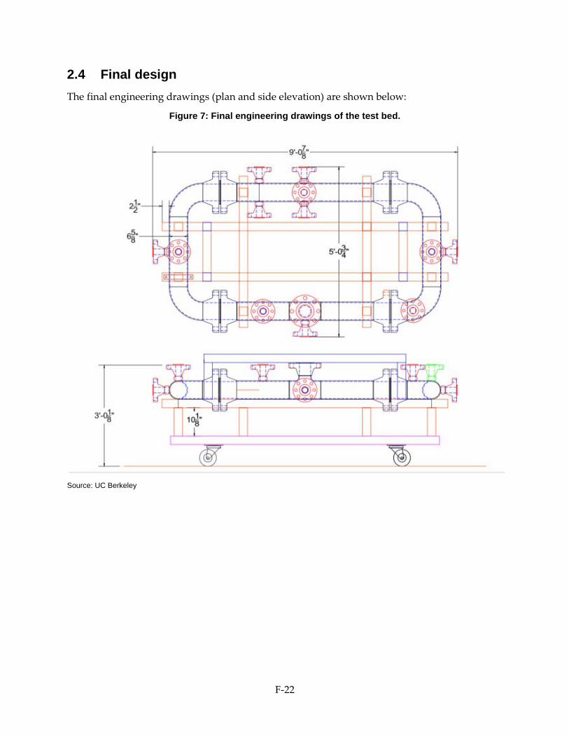
2.4 Final design The final engineering drawings (plan and side elevation) are shown below:

Figure 7: Final engineering drawings of the test bed.

Source: UC Berkeley

F-22

CHAPTER 3: Fabrication 3.1 Bidding process The UC Berkeley research team had several meetings throughout September, October, and early November 2013 discussing the test bed, and consulting with several entities (such as heads of the Mechanical Engineering (ME) and EECS machine shops, environmental health and safety on campus). Initially, the researchers decided to have the test bed constructed off campus by subcontractors for lab safety and liability reasons. The liability regarding specialized welding of pressurized pipes was especially key to this decision, since the project requires certified welders contracted for the test bed construction.

The head of the EECS shop provided several names. The research team sent out the bidding document request for quotation by email to four companies: Lake Engineering, Nor Cal Metal Fabricators, Roy E. Hanson Jr. Manufacturing, and Vertex FD. Vertex FD replied that they could not bid the project because they don’t work on this size of pipe. There were several questions regarding the fabrication: the type of pressure relief valves, and the expected longevity of the test bed (affects the fabrication and testing). One bidder suggested that the test bed design change to allow elbow pieces of pipe at the ends instead of a continuous curved piece for easier and cheaper fabrication. After a month of discussion, Nor Cal declined to bid, stating there were elements of the project for which the company could not perform (e.g., the certified welding). The researchers received two viable quotes from Hanson Tank and Lake Engineering.

On December 19, the research team met to discuss the bids. The bid from Hanson Tank did not include the standard operating instructions, did not include the detailed break down of labor and materials that was requested, did not include the sensors and valves as part of the project, did not include hydrotesting, charged $5000 more for completing within 4 weeks, and did not provide proof of welding certification. Lake Engineering did not provide physical address nor experience as Lake Engineering, nor amount of time to complete the project. Of the work that was comparable to what Hanson Tank outlined, the Lake Engineering bid (nearly $33k) was within $1000 of Hanson Tank bid.

After much thought, the researchers decided to have the EECS machine shop on campus fabricate the test bed, using subcontractors for the certified welding and hydrotesting.

F-23

3.2 Process of fabrication Figure 8: The welded pieces of the test bed.

Source: UC Berkeley

F-24

Figure 9: Straight section of the welded pieces of the test bed, showing the insertion ports.

Source: UC Berkeley

Figure 10: The welded curved ends and straight sections of the test bed.

Source: UC Berkeley

F-25

3.3 Validation tests The test bed must undergo similar tests as natural gas pipelines. One test is pressure testing, (described in Part 192, Subpart J7) and Spike methods, which use pressurized water to test the pipeline at Maximum Allowable Operating Pressure (MAOP) or several times greater than MAOP before it can go into service. A drop in pressure indicates a defect. Before the vessel can be pressure tested, it must undergo X-rays provide the ability to determine the integrity of the weld (per Part 192 Subpart E10 - Welding of Steel in Pipelines, see http://ecfr.gpoaccess.gov/cgi/t/text/text-idx?c=ecfr&sid=69ffb827c050d6f88db61f0d9cc47552&rgn=div6&view=text&node=49:3.1.1.1.8.5&idno=49). Other tests is Magnetic Particle Inspection (for surface and slightly subsurface material discontinuity) and Dye Penetration Inspection (used to detect surface defects); this is part of ASME SEC. V ART.6 criteria B31.1.

All welds were X-rayed by MISTRAS service division. Initially, the welds did not pass and had to be redone. Finally, all 6 inch diameter welds passed the ASME 831.1 criteria.

All 24 two-inch and one four-inch welds passed the Magnetic Particle Inspection and Dye Penetration Inspection, necessary for the containment of 1350 psi of Natural Gas.

The test bed was then Hydro-tested. This test is an eight hour long pressure test taking the system first to 2200 psi and then 2300 psi. These pressures exceed the MAOP of the test bed, which is 1350 psi. The multiplying factor for Natural Gas is 66.6%, which is set by the Department of Transportation for vessels in public areas and carrying natural gas. Thus the vessel was tested at 2200psi; multiplied by 66.6% is 1465.2psi. This exceeds 1350 psi, because a "window" of pressure is required for thermal expansion. An additional 100 psi will afford plenty of flexibility, based on the volume of the system. The test bed successfully passed hydro testing.

The final step was to powder coat the vessel. This led to some complications, as the flanges were gouged upon delivery, and some portions of the test bed were not masked properly. The gouged flanges were machined and the flanges were re-powder coated (albeit the incorrect color).

F-26

Figure 11: Assembled test bed.

Souce: UC Berkeley

F-27

CHAPTER 4: Installation The pieces were delivered and assembled in nearby Davis Hall since it has a crane to ease assembly.

Figure 12: The installed test bed in 143 Sutardja Dai Hall. The locked cabinet with the compressed air tanks is shown in the right corner.

Source: UC Berkeley

F-28

Figure 13: The tube from the compressed air tanks runs along the floor (left), under a wood protector, and then up to the test bed (right).

Source: UC Berkeley

The compressed gas tanks were installed in a locked cabinet (Figure 12), and the tubes connected to the test bed (Figure 13).

A new 208V receptacle was installed for the fan motor, but ended up not used as the researchers found a motor that ran on 120V.

F-29

Figure 14: Commercial pressure sensor.

Source: UC Berkeley

A simple commercial pressure sensor was installed (Figure 14) and a commercial flow sensor with flow conditioners installed (early October).

F-30

Figure 15: Test port with electrical feedthroughs is the sensor insertion point into the test bed.

Source: UC Berkeley

Electrical feedthroughs were installed and finally the Pressure and Flow MEMS sensors installed. The results of the tests will be reported separately.

F-31

APPENDIX A: Maximum Operating Pressure (MAAOP) calculation:

F-32

APPENDIX G: Sensor Testing in the Test Bed

G-1

NOVE MBER 2014 CE C-500-2014-XXX

PREPARED BY: Primary Author(s): Pit Pillatsch Son Duy Nguyen Paul Wright Richard White Jim Evans Igor Paprotny Sean Wihera Therese Peffer The Regents of the University of California University of California, Berkeley Berkeley, CA 94720 Phone: 510-643-1440 | Fax: 510-643-9324 http://ame.berkeley.edu Contract Number: 500-10-044 Prepared for: California Energy Commission Avtar Bining, PhD Contract Manager Fernando Pina Office Manager Energy Systems Research Office Laurie ten Hope Deputy Director ENERGY RESEARCH AND DEVELOPMENT DIVISION Robert P. Oglesby Executive Director

DISCLAIMER This report was prepared as the result of work sponsored by the California Energy Commission. It does not necessarily represent the views of the Energy Commission, its employees or the State of California. The Energy Commission, the State of California, its employees, contractors and subcontractors make no warranty, express or implied, and assume no legal liability for the information in this report; nor does any party represent that the uses of this information will not infringe upon privately owned rights. This report has not been approved or disapproved by the California Energy Commission nor has the California Energy Commission passed upon the accuracy or adequacy of the information in this report.

G-2

ACKNOWLEDGEMENTS



G-3

PREFACE

The California Energy Commission Energy Research and Development Division supports public interest energy research and development that will help improve the quality of life in California by bringing environmentally safe, affordable, and reliable energy services and products to the marketplace.

The Energy Research and Development Division conducts public interest research, development, and demonstration (RD&D) projects to benefit California.

The Energy Research and Development Division strives to conduct the most promising public interest energy research by partnering with RD&D entities, including individuals, businesses, utilities, and public or private research institutions.

Energy Research and Development Division funding efforts are focused on the following RD&D program areas:








• Transportation

Sensor Testing in the Test Bed Report is an interim report for the Natural Gas Pipeline Sensors project (contract number 500-10-044) conducted by The Regents of the University of California. The information from this project contributes to Energy Research and Development Division’s Energy Systems Integration Program.

For more information about the Energy Research and Development Division, please visit the Energy Commission’s website at www.energy.ca.gov/research/ or contact the Energy Commission at 916-327-1551.

G-4


ABSTRACT

The purpose of the natural gas pipeline sensor project is to develop low-cost wireless sensors that can instrument and increase the reliability and safety of natural gas pipelines using existing access points on the pipeline such as valve stations. This report describes the testing of the flow and pressure micro-electro-mechanical systems (MEMS) sensors in the University of California, Berkeley (UCB) fabricated test bed. The test bed is a “racetrack” oval (roughly four feet by eight feet) of six-inch diameter pipe that provides an inert laboratory environment to emulate natural gas pipelines in field conditions. The test bed has many ports perpendicular to the flow that allow the insertion of the sensors; electrical feedthroughs provide the communication to monitoring equipment. The output of the prototype sensors was compared to that of commercial sensors for validation.



Pillatsch, Pit, Sean Wihera, Son Duy Nguyen, Paul Wright, Richard M. White, Jim Evans, Sean Wihera, Therese Peffer. (University of California, Berkeley). 2014. Sensor testing in the test bed. California Energy Commission. Publication number: CEC-XXX-2014-XXX.

G-5

TABLE OF CONTENTS


PREFACE .................................................................................................................................................... 4

ABSTRACT ................................................................................................................................................ 5


LIST OF FIGURES .................................................................................................................................... 7

EXECUTIVE SUMMARY ........................................................................................................................ 8


1.1 Initial Flow Sensor Experiments ................................................................................................. 9

CHAPTER 2: Test Bed Measurement Procedure ............................................................................... 12

2.1 Pressure Measurements ............................................................................................................. 12

2.2 Flow Measurements ................................................................................................................... 16

G-6

LIST OF FIGURES

Figure 1: Initial measurement apparatus for flow sensors 10 Figure 2: Comparison between experimental flow measurements and simulation prediction 11 Figure 3: Sensor mounting for experiments inside the test bed 12 Figure 4: Reference pressure monitor 13 Figure 5: Air cylinder cabinet and pressure settings 14 Figure 6: Air flow control dial for pressurizing and venting the test bed 14 Figure 7: Pressure relief and safety system 15 Figure 8: Precision component analyser and electrical feedthroughs for the sensors. 16 Figure 9: Direct Current power supply for the fan 17 Figure 10: Electrical feedthroughs for the internal fan motor 18 Figure 11: Electronic speed control for the internal fan 19 Figure 12: Commercial reference flow meter 20

G-7

EXECUTIVE SUMMARY

The purpose of the natural gas pipeline sensor project is to develop low-cost miniature wireless sensors that can instrument and increase the reliability and safety of natural gas pipelines using existing access points on the pipeline such as valve stations. This project developed prototype micro-electro-mechanical systems (MEMS) flow and pressure sensors in a laboratory at the University of California, Berkeley. To ensure reliable performance in the field, these sensors must be tested in a way that emulates the natural gas pipeline environment yet is safe for the researchers.

The goal is to test the micro-electro-mechanical systems (MEMS) sensors in a safe convenient location for the researchers that still provides a realistic emulation of natural gas pipelines in the field.

The objective is to describe the procedure of testing the MEMS flow and pressure sensors in a test bed fabricated by UC Berkeley. The test bed is a “racetrack” oval (roughly four feet by eight feet) of six-inch diameter pipe that provides an inert laboratory environment to emulate natural gas pipelines in field conditions. The external ports of the test bed allow researchers to insert the sensors into the test bed; electrical feedthroughs provide the infrastructure to measure the sensor output. The output of the sensors was compared with the output of commercial sensor

G-8

CHAPTER 1: Introduction The purpose of the natural gas pipeline sensor project is to develop low-cost miniature wireless sensors that can instrument and increase the reliability and safety of natural gas pipelines using existing access points on the pipeline such as valve stations. This project developed prototype micro-electro-mechanical systems (MEMS) flow and pressure sensors in a laboratory at the University of California, Berkeley. To ensure reliable performance in the field, these sensors must be tested in a way that emulates the natural gas pipeline environment yet is safe for the researchers.

The goal is to test the micro-electro-mechanical systems (MEMS) sensors in a safe convenient location for the researchers that still provides a realistic emulation of natural gas pipelines in the field.

The objective is to describe the procedure of testing the MEMS flow and pressure sensors in the UC Berkeley fabricated test bed. The Electrical Engineering and Computer Science machine shop fabricated a closed loop test bed that was located on campus for convenient access by the researchers. The test bed was a self-contained apparatus in the shape of a “racetrack” oval (roughly four feet by eight feet) of six-inch pipe situated on a rolling table. The test bed includes pressurized tanks, ports for viewing or accommodating test sensors, commercial gas velocity measurements (velocimetry), pressure and flow sensors, a in-flow fan, and safety features. The ports into the piping would accommodate small test sensors for variables such as micro-electrical-mechanical systems (MEMS) gas pressure and flow velocity sensors.

The sensors were coupled to typical laboratory test instruments (such as oscilloscopes and lab power supplies). The researchers decided that the maximum pressure employed in laboratory testing on campus would be limited to 400 pounds per square inch (psi) due to safety concerns.

1.1 Initial Flow Sensor Experiments Before the completion of the test bed, the researchers developed a method for the initial testing of the MEMS-based flow sensors (Figure 1). The main part of the apparatus consists of an open- ended 6-inch inner diameter air duct connected to a large fan. The configuration allows for flow variation through a transformer. A commercial anemometer is used to determine the achieved flow velocities and to provide a reference. After establishing these initial parameters, the anemometer is replaced by the MEMS-fabricated flow sensor. An Agilent precision LCR (inductance (L), capacitance (C), and resistance (R)) component analyser is used to record the changes in capacitance of the flow sensor with respect to flow velocity. The data is recorded and visualized through a connection between the LCR meter and a personal computer. Given that these measurements are taking place in an open- ended section of pipe, the arrangement does

G-9

not allow control over the internal pipe pressure and so the results are taken in atmospheric pressure.

Figure 1: Initial measurement apparatus for flow sensors

Photo Credit: UC Berkeley

G-10

The figure below shows the experimental results achieved with this method. The particular flow sensor presented was adjusted for atmospheric pressure during fabrication. The solid blue line is based on design simulations. The red and yellow triangles correspind to actual measurements at a range of flow velocities from 0 up to 20 meters per second (m/s). The experiment shows very good agreement with the model prediction.

Figure 2: Comparison between experimental flow measurements and simulation prediction

Source: UC Berkeley

0 5 10 15 20

9.7

9.8

9.9

10

10.1

10.2

10.3

10.4

Velocity [m/s]

Capa

cita

nce

[pF]

experimentsanalysis

G-11

CHAPTER 2: Test Bed Measurement Procedure 2.1 Pressure Measurements The first measurements taken in the specifically designed gas sensor test bed, as described in the previous report, were using the MEMS pressure sensors. This section describes the employed measurement procedure and safety precautions.

Figure 3 shows the arrangement of flow and pressure sensors as they are mounted inside the test bed. A metal rod has fixtures to accommodate both sensor types and the length is such that the flow sensor reaches the center of the 6-inch pipe. Furthermore, the electrical connections to the external measurement equipment are achieved through pressure resistent feedthroughs that go through the plate of the mounting flange.

Figure 3: Sensor mounting for experiments inside the test bed

Source: UC Berkeley

The reference pressure gauge is depicted in Figure 4. It is mounted onto the flange closest to the sensor insertion point and gives a direct reading of the pressure inside the test bed. It is important to note that the dial indicates the pressure in pressure per square inch (psi), meaning that a pressure of 0 psi indicates atmospheric pressure.

G-12

Figure 4: Reference pressure monitor

Source: UC Berkeley

The pressure to the test bed is provided through compressed air cylinders. These cylinders have a maximum pressure of 2000 psi, thus far exceeding the maximum test bed pressure of 200 psi. In order to avoid over-pressurization, several safety mechanisms are in place. The gas cylinders are placed inside a locked cabinet. After the initial set-up where the pressure is down-regulated to 200 psi, as seen in Figure 5, the cabinet is locked and the user only has control over the external dials (Figure 6) that allow opening the air flow to pressurize the test bed or to vent it.

G-13

Figure 5: Air cylinder cabinet and pressure settings

Source: UC Berkeley

Figure 6: Air flow control dial for pressurizing and venting the test bed

Source: UC Berkeley

In addition to this limited user control, a pressure relief valve, Figure 7, is installed. Should the pressure inside the test bed unexpectedly rise above 200 psi, this valve will open up and vent the pressure gradually. In an extreme situation where the pressure rises above 210 psi, the relief valve has an internal burst disk that will rupture and release the pressure in the test bed.

G-14

Figure 7: Pressure relief and safety system

Source: UC Berkeley

Figure 8 depicts the electrical connection to the same precision LCR component analyser described above by clamping to the cable coming out of the high pressure feedthrough. This piece of equipment enables measuring of the capacitance changes of the MEMS pressure sensor in relation to a pressure increase in the pipeline test bed as monitored by the reference pressure gauge.

G-15

Figure 8: Precision component analyser and electrical feedthroughs for the sensors.

Source: UC Berkeley

2.2 Flow Measurements An internal fan is installed inside the test bed in order to generate flow at pressure for testing of the miniature MEMS-based flow sensors. The internal fan operates on Direct Current (DC) power and is specified to be able to withstand up to 5 kilowatts of power. In order to achieve this, a large external DC power supply, running off a 208 Volt three-phase mains plug is necessary, depicted in the figure below.

G-16

Figure 9: Direct Current power supply for the fan

Source: UC Berkeley

The connections to the fan motor are again done through pressure resistant feedthroughs as shown in the figure below. The difference to the sensor connections is that these are not only signal wires, they need to be able to withstand a large DC current, which is why the wire gauge is selected significantly thicker.

G-17

Figure 10: Electrical feedthroughs for the internal fan motor

Source: UC Berkeley

The fan speed can be adjusted continuously through the Electronic Speed Control (ESC) system shown in Figure 11. This unit converts the DC power coming from the main power supply and takes care of the necessary commutation for the brushless electrical fan motor. The reasons for using a brushless motor are the generally higher power densities and outstanding robustness. Furthermore, brushed motors have a tendency to create sparks due to the mechanical commutation. Using brushless technology eliminates this problem.

G-18

Figure 11: Electronic speed control for the internal fan

Source: UC Berkeley

Finally, Figure 12 depicts the arrangement of a commercial, insertion based reference flow meter by Sage metering. The positioning of this meter is exactly symmetrical to the location of the MEMS based flow meter. Both meter and sensor are preceded by flow conditioners on either side of the test bed to ensure consistency of the flow conditions experienced by both. The Sage meter gives a reading of the volumetric flow in standard cubic feet per minute, which can then be converted into meters per second.

G-19

Figure 12: Commercial reference flow meter

Source: UC Berkeley

The measurement results will be discussed in the following report.

G-20

APPENDIX H: Data Analysis of Sensor Testing

H-1



H-2

ACKNOWLEDGEMENTS



H-3

PREFACE












• Transportation

Data Analysis of Sensor Testing is an interim report for the Natural Gas Pipeline Sensors project (contract number 500-10-044) conducted by The Regents of the University of California. The information from this project contributes to Energy Research and Development Division’s Energy Systems Integration Program.


H-4


ABSTRACT

The purpose of the natural gas pipeline sensor project is to develop low-cost wireless sensors that can instrument and increase the reliability and safety of natural gas pipelines using existing access points on the pipeline such as valve stations. This report describes the analysis of the testing of the flow and pressure micro-electro-mechanical systems (MEMS) sensors in the University of California, Berkeley (UCB) fabricated test bed. The test bed is a “racetrack” oval (roughly four feet by eight feet) of six-inch diameter pipe that provides an inert laboratory environment to emulate natural gas pipelines in field conditions.

The initial test results of the pressure sensors revealed two issues: low sensitivity and an unexpected difference in output between increasing pressure and decreasing pressure. The researchers hypothesized these issues stemmed from a leak in the seals around the diaphragm, and modified the design. The subsequent testing of the pressure sensors showed that the design modification fixed both issues. The data showed appropriate sensitivity, and accurate measure of pressure whether under increasing or decreasing conditions; repeatability of these tests indicates the reliability of the pressure sensors. The initial tests of the flow sensors found that particles from the interior of the test bed disrupted the measurement; future designs of this sensor may use magnets to eliminate the typical iron particles from interfering with the flow sensor mechanism.



Pillatsch, Pit, Sean Wihera, Son Duy Nguyen, Paul Wright, Richard M. White, Jim Evans, Sean Wihera, Therese Peffer. (University of California, Berkeley). 2014. Data analysis of sensor testing. California Energy Commission. Publication number: CEC-XXX-2014-XXX.

H-5

TABLE OF CONTENTS


PREFACE .................................................................................................................................................... 4

ABSTRACT ................................................................................................................................................ 5


LIST OF FIGURES .................................................................................................................................... 7


CHAPTER 1: Introduction .................................................................................................................... 10

CHAPTER 2: Pressure Sensors ............................................................................................................ 11

2.1 Initial Test Results ....................................................................................................................... 11

2.2 Discussion and Design Changes ............................................................................................... 13

2.3 Updated Pressure Sensor Results ............................................................................................. 16

CHAPTER 3: Flow Sensors .................................................................................................................... 19


H-6

LIST OF FIGURES

Figure 1: Simulation calculation of capacitance as a function of pressure 11 Figure 2: Experimental data of capacitance when increasing the pressure 12 Figure 3: Experimental data of capacitance when increasing, holding, then decreasing pressure 13 Figure 4: Miniature pressure sensor layout 14 Figure 5: Schematic of a single membrane arrangement of the miniature pressure sensor 14 Figure 6: Cross section of a single pressure sensor membrane at the dotted red line in Figure 5 15 Figure 7: Micrograph of cross-section cut of a fabricated pressure sensor 15 Figure 8: Updated pressure sensor experimental data for a pressure increase 16 Figure 9: Data for updated sensor during increasing and decreasing pressure 17 Figure 10: Linear curve fit to the experimental pressure data 17 Figure 11: Quadratic curve fit to the experimental data 18

H-7

EXECUTIVE SUMMARY

The purpose of the natural gas pipeline sensor project is to develop low-cost miniature wireless sensors that can instrument and increase the reliability and safety of natural gas pipelines using existing access points on the pipeline such as valve stations. This project developed prototype micro-electro-mechanical systems (MEMS) flow and pressure sensors in a laboratory at the University of California, Berkeley (UCB). To ensure reliable performance in the field, these sensors must be tested in a way that emulates the natural gas pipeline environment yet is safe for the researchers.

The goal is to analyze the testing of the micro-electro-mechanical systems (MEMS) sensors in the test bed developed by UC Berkeley. No field testing sites were available for testing.

The objective is to describe the analysis of the sensor testing solely in the test bed, since field testing was not possible. The test bed is a “racetrack” oval (roughly four feet by eight feet) of six-inch diameter pipe that provides an inert laboratory environment to emulate natural gas pipelines in field conditions. The external ports of the test bed allow researchers to insert the sensors into the test bed. The output of the sensors was compared with the output of commercial sensors. The analysis included sensitivity, accuracy, and reliability.

The initial test results of the pressure sensors revealed two issues: low sensitivity and an unexpected difference in output between increasing pressure and decreasing pressure. The researchers hypothesized these issues stemmed from a leak in the seals around the diaphragm, and modified the design. The subsequent testing of the pressure sensors showed that the design modification fixed both issues. The data showed appropriate sensitivity, and accurate measure of pressure whether under increasing or decreasing conditions; repeatability of these tests indicates the reliability of the pressure sensors.

H-8

A blank page is inserted to insure Chapter 1 starts on an odd number page. Blank pages are not labeled.

H-9


The goal of is to analyze the testing of the micro-electro-mechanical systems (MEMS) sensors in the test bed developed by UC Berkeley. No field testing sites were available for testing.

The objective of is to describe the analysis of the sensor testing solely in the test bed, since field testing was not possible. The test bed is a “racetrack” oval (roughly four feet by eight feet) of six-inch diameter pipe that provides an inert laboratory environment to emulate natural gas pipelines in field conditions. The external ports of the test bed allow researchers to insert the sensors into the test bed. The sensors were coupled to typical laboratory test instruments (such as oscilloscopes and lab power supplies). The researchers decided that the maximum pressure employed in laboratory testing on campus would be limited to 400 pounds per square inch (psi) due to safety concerns.

The output of the sensors was compared with the output of commercial sensors. The analysis included sensitivity, accuracy, and reliability.

H-10

CHAPTER 2: Pressure Sensors The experimental procedure for testing the MEMS pressure sensors in the gas test bed was presented in a previous report. This report discusses measurement results and improvements made after initial testing.

2.1 Initial Test Results Figure 1 depicts Finite Element Method (FEM) simulation results for the behavior of a MEMS pressure sensor when the pressure inside the gas test bed is increased from 0 to 200 pounds per square inch (psi). The increase in capacitance as a function of pressure over that range was calculated to be 8 picofarads (pF), starting at approximately 57 pF.

Figure 1: Simulation calculation of capacitance as a function of pressure

Source: UC Berkeley

In contrast, Figure 2 shows the first experimental data acquired in the test bed. The general shape of the curve matches the calculation. However, the increase in capacitance is only in the order of 100 femptofarad (fF). Furthermore, the curve only starts at approximately 65.34 pF. The result is a low sensitivity (0.00056 pF/psi) of the measurements. Such small changes in capacitance are difficult to record accurately.

0 50 100 150 20056

58

60

62

64

66

Pressure [PSI]

Cap

acita

nce

[pF]

H-11

Figure 2: Experimental data of capacitance when increasing the pressure

Source: UC Berkeley

In addition, Figure 3 shows the result of an experiment, where the pressure was first gradually increased from 0 to 200 psi. Then, the pressure inside the test bed was kept at 200 psi for 20 minutes, before gradually releasing the pressure. A substantial drop in capacitance of about 70 fF on the MEMS sensor can be seen in the graph. This is not supposed to happen as the reference pressure sensor on the test bed indicated a constant level of 200 psi during this period. The results show a strong hysterisis for the pressure release as compared to the pressure increase.

H-12

Figure 3: Experimental data of capacitance when increasing, holding, then decreasing pressure

Source: UC Berkeley

2.2 Discussion and Design Changes As discussed, the initial measurements on the MEMS pressure sensor did not provide satisfactory results. The reasons for this will be analyzed in this section. First, Figure 4 serves as a reminder of how the pressure sensor works. It is composed of an array of small, round pressure capsules that have a vacuum inside. Under pressure the top membrane deflects inwards and the capacitance between the bottom electrode and this top membrance changes as a consequence.

H-13

Figure 4: Miniature pressure sensor layout

Source: UC Berkeley

Figure 5 shows a magnified schematic of a single pressure capsule. Silicon dioxide (SiO2) serves as a sealing layer to close the internal vacuum against the external pressure. The dashed red line indicates a section cut as it can be seen in Figure 6.

Figure 5: Schematic of a single membrane arrangement of the miniature pressure sensor

Source: UC Berkeley

H-14

The strong hysteresis observed supported the hypothesis that the sealing of the capsules was not succesful. While the test bed and the MEMS pressure sensors were at 200 psi, air from inside the test bed slowly leaked into the chamber of the capsules and caused the drop in capacitance observed in Figure 3.

Figure 6: Cross section of a single pressure sensor membrane at the dotted red line in Figure 5

Source: UC Berkeley

This is confirmed by the micrograph in Figure 7. It shows a cross section view of an actual pressure sensor with the Low Temperature Oxide (LTO) layer, the membrane and the substrate. A void in the sealing can easily be discerned.

Figure 7: Micrograph of cross-section cut of a fabricated pressure sensor

Source: UC Berkeley

H-15

As a result the fabrication process for the MEMS pressure sensors was adjusted. The second layer of silicon nitride (Si3N4), shown in green in Figure 6, was omitted and the thickness of the oxide sealing layer was increased.

2.3 Updated Pressure Sensor Results The previously discussed changes in the device fabrication have a dramatic effect on the achieved experimental results from the pressure sensors. Figure 8 shows an experiment with an increase in pressure as it was shown before but with the improved pressure sensor. The initial capacitance has now increased to about 114 pF, which is believed to be due to a reduction in parasitic capacitance as a consequence of the improved processing. The measurement range now shows a difference of 23.3 pF, which is two orders of magnitude larger than the previous experiment and better than the simulation prediction. This dramatically increases sensitivity (0.131 pF/psi) of the sensors and makes readout far less complicated.

Figure 8: Updated pressure sensor experimental data for a pressure increase

Source: UC Berkeley

Additionally, Figure 21 shows the same experiment that was conducted earlier, where the pressure is first increased inside the testbed and then held at 200 psi before being released. There is no discernible hysteresis anymore and the results for an increase and a decrease in pressure match very closely with only a 1% difference.

H-16

Figure 9: Data for updated sensor during increasing and decreasing pressure

Source: UC Berkeley

Figure 10 and Figure 11 show a linear and a quadratic curve fit to the experimental data. As expected, the quadratic curve fit is more accurate with only a 0.9 % average error compared to 3.3 % average error for the linear fit.

Figure 10: Linear curve fit to the experimental pressure data

Source: UC Berkeley

H-17

Figure 11: Quadratic curve fit to the experimental data

Source: UC Berkeley

H-18

CHAPTER 3: Flow Sensors The initial tests of the flow sensors in the test bed found that particles from the interior of the test bed got caught in the fine capacitor fingers of the flow meter. While the flow sensor function was shown in the laboratory, the flow sensor has not rendered data in the test bed. The research team discussed the redesign of the flow sensor as a potential fix. Future designs of this sensor may use magnets to draw the typical iron particles away from the flow and prevent particles from interfering with the flow sensor mechanism.

H-19

CHAPTER 4: Conclusions This report shows experimental results for MEMS pressure and flow sensors performed inside the gas test bed. Initial results showed problems. For the pressure sensors, the problem was in the fabrication process of the devices. Data analysis showed that the problems were caused by defects in the sealing of the pressure capsules on the MEMS sensors. Consequently, the fabrication process was adjusted to improve this sealing, resulting in great sensor performance, reproducibility and sensitivity in the updated devices during a subsequent experiment. For the flow sensors, the problem was iron particles caught in the capacitive fingers of the sensor. Future designs may use magnets to draw the iron particles out of the path of flow.

H-20

APPENDIX I: Miniaturization and Lifetime Testing of Sensors

I-1



I-2

ACKNOWLEDGEMENTS



I-3

PREFACE












• Transportation

Miniaturization and Lifetime Testing of Sensor is an interim report for the Natural Gas Pipeline Sensors project (contract number 500-10-044) conducted by The Regents of the University of California. The information from this project contributes to Energy Research and Development Division’s Energy Systems Integration Program.


I-4


ABSTRACT

The purpose of the natural gas pipeline sensor project is to develop low-cost wireless sensors that can instrument and increase the reliability and safety of natural gas pipelines. This report describes the further miniaturization and lifetime testing of the flow and pressure micro-electro-mechanical systems (MEMS) sensors.

The researchers concluded that the current dimensions of the sensors are already very small and could only be reduced by a significant effort in fabrication process and tool development. Thus, accelerated erosion testing was performed using sandblasting equipment; the Silicon Carbide coating on the flow sensor dramatically reduced the erosion damage. The flow sensor was tested at temperatures ranging from 23 Celcius (C) to 43 C, at three different air flow rates; the output different by less than 0.5%. The researchers explored several options for inserting these MEMS sensors into a natural gas pipeline, such as hot tapping (inserting a test point site while the pipe is in service) and Smart Balls (foam balls with acoustic sensors that float through the pipeline. The researchers concluded that the current access points at valve sites and metering stations are appropriate for inserting the MEMS sensors.



Pillatsch, Pit, Sean Wihera, Son Duy Nguyen, Paul Wright, Richard M. White, Jim Evans, Sean Wihera, Therese Peffer. (University of California, Berkeley). 2014. Miniaturization and Lifetime Testing of Sensor. California Energy Commission. Publication number: CEC-XXX-2014-XXX.

I-5

TABLE OF CONTENTS


PREFACE .................................................................................................................................................... 4

ABSTRACT ................................................................................................................................................ 5


LIST OF FIGURES .................................................................................. Error! Bookmark not defined.



CHAPTER 2: Further Miniaturization ............................................................................................... 10

CHAPTER 3: Accelerated Lifetime Testing ....................................................................................... 11

3.1 Abrasive Particles ....................................................................................................................... 11

3.2 Temperature Fluctuations ......................................................................................................... 17

CHAPTER 4: Low-Cost Insertion Points ............................................................................................ 19

4.1 Hot Tapping ................................................................................................................................ 19

4.2 SmartBall ...................................................................................................................................... 19

4.3 Discussion .................................................................................................................................... 19

Reference .................................................................................................................................................. 21

I-6

EXECUTIVE SUMMARY

The purpose of the natural gas pipeline sensor project is to develop low-cost miniature wireless sensors that can instrument and increase the reliability and safety of natural gas pipelines using existing access points on the pipeline such as valve stations. This project developed prototype micro-electro-mechanical systems (MEMS) flow and pressure sensors in a laboratory at the University of California, Berkeley (UCB). To ensure reliable performance in the field, these sensors must be tested in a way that emulates the natural gas pipeline environment yet is safe for the researchers.

The goal is to discuss the further miniaturization of the sensors and the accelerated lifetime testing of the sensors. The researchers concluded that the 5 millimeter by 5 millimeter dimensions of each sensor are already very small and could only be reduced by a significant effort in fabrication process and tool development.

The objective is to refine the designs of the sensors for optimum production, resilience in the field (especially with respect to erosion and temperature ranges), and explore low-cost insertion techniques.

With regard to further miniaturization, the researchers concluded that the 5 millimeter by 5 millimeter dimensions of each sensor are already very small and could only be reduced by a significant effort in fabrication process and tool development. The researchers decided not to perform aggressive erosion testing in the test bed due to concerns over internal damage and safety. Thus, accelerated erosion testing was performed using sandblasting equipment; the Silicon Carbide coating on the flow sensor dramatically reduced the erosion damage. The flow sensor was tested at temperatures ranging from 23 Celcius (C) to 43 C, at three different air flow rates; the output different by less than 0.5%. The researchers explored several options for inserting these MEMS sensors into a natural gas pipeline, such as hot tapping (inserting a test point site while the pipe is in service) and Smart Balls (foam balls with acoustic sensors that float through the pipeline. The researchers concluded that the current access points at valve sites and metering stations are appropriate for inserting the MEMS sensors.

I-7

A blank page is inserted to insure Chapter 1 starts on an odd number page. Blank pages are not labeled.

I-8


The goal is to discuss the further miniaturization of the sensors and the accelerated lifetime testing of the sensors.

The objective is to refine the designs of the sensors for optimum production, resilience in the field (especially with respect to erosion and temperature ranges), and explore low-cost insertion techniques.

I-9

CHAPTER 2: Further Miniaturization As can be seen in Figure 1, the dimensions of the MEMS flow sensor die are about 5x5 mm. The dimensions for the pressure sensor are similar to this. These dimensions are already very small and could only be reduced by a significant effort in fabrication process and tool development. The masks that are used for the current versions could not be utilized any longer and a complete redesign and financial investment would be required. Furthermore the advantages of further downscaling are considered very small with regards to the potential risks of decreased sensitivity and durability.

Figure 1: Close-up of sample preparation of flow sensors

Source: UC Berkeley

I-10

CHAPTER 3: Accelerated Lifetime Testing The sensors were tested to ensure resilience in the field, especially with respect to erosion from abrasive particles and temperature fluctuations.

3.1 Abrasive Particles The main concern for sensor operation inside pipelines is the presence of abrasive particles such as sand that are carried by the flow. The flow sensors are at a greater risk because they are positioned in the center of the pipeline where the exposure and the flow velocity are greatest. The pressure sensors in comparison can be placed anywhere in the pipe, even in the recessed and sheltered areas provided at flanged access points.

Different size and density particles take different paths inside a pipeline when they encounter an elbow, according to Barton (2013). Small light particles tend to follow the flow uniformly, while medium particles tend to concentrate toward the edge of the pipe away from the inner curve after travelling through the elbow. Large, heavy particles ricochet off the edge of the pipe as they flow around the elbow. This demonstrates the difficulty of estimating erosion if particle size distribution is unknown. In general, heavier particles cause more damage inside pipelines due to collision with the sidewalls. This project considers the impact of particles on MEMS based flow sensors.

The researchers decided not to perform aggressive erosion testing in the test bed due to concerns over internal damage and safety. Thus, accelerated erosion testing is performed using Industrial Cleaning Machines (ICM) Superhone sandblasting equipment, Figure 100. Due to the high air flow (30-50 meters per second (m/s)), high density particles (100-mesh) and high nozzle pressure (30 pounds per square inch (psi)) this treatment is far more abrasive than what could realistically be expected inside a pipeline.

Each test was therefore conducted over a very short period of time, 1-2 minutes, and in a distance of 15-30 centimeters (cm) from the nozzle.

I-11

Figure 2: Sandblasting tool

Source: UC Berkeley

Figiure 3 illustrates an additional abrasion resistant silicon carbide (SiC) coating that was deposited during fabrication of the flow sensors (green layer). This coating faces the on-coming particles and increases wear performance.

I-12

Figure 3: Erosion resistant Silicon Carbide coating

Source: UC Berkeley

Both versions of the flow sensors, with and without SiC coating, were fabricated and tested during this study. Figure 4 illustrates the sample preparation were three sets of coated and uncoated sensors are bonded onto individual glass slides.

Figure 4: Sample preparation, three sets of samples each with and without coating

Source: UC Berkeley

Figure 5 provides a close up view of a test sample, the SiC coating does have a distinctive green color that can be seen on the left hand sensor.

I-13

Figure 5: Close-up of sample preparation: devices with and without coating

Source: UC Berkeley

Figure 6, Figure 7 and Figure 8 are micrographs of the samples after sandblasting. The results in Figure 6 are performed with a nozzle distance of 30 cm. The SiC coated device withstands this treatment much better than the uncoated version. In the uncoated device, most of the capacitor fingers are completely broken off, whereas a large proportion of the fingers on the coated version are still intact.

I-14

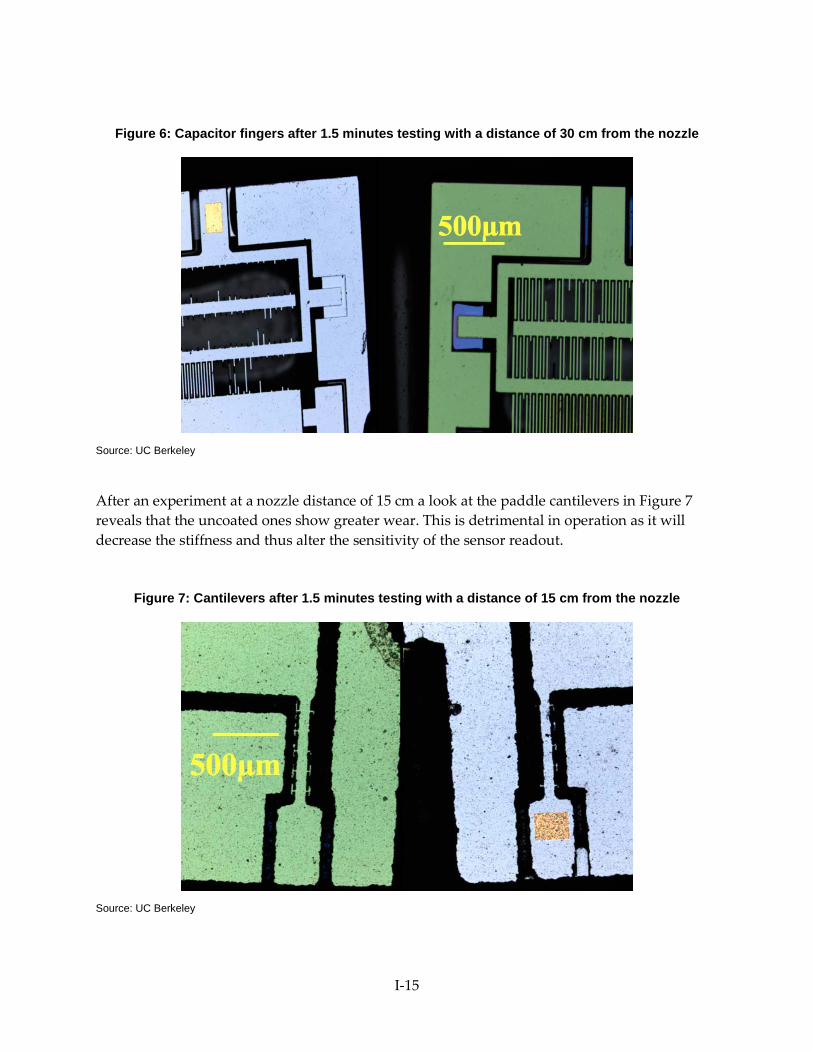
Figure 6: Capacitor fingers after 1.5 minutes testing with a distance of 30 cm from the nozzle

Source: UC Berkeley

After an experiment at a nozzle distance of 15 cm a look at the paddle cantilevers in Figure 7 reveals that the uncoated ones show greater wear. This is detrimental in operation as it will decrease the stiffness and thus alter the sensitivity of the sensor readout.

Figure 7: Cantilevers after 1.5 minutes testing with a distance of 15 cm from the nozzle

Source: UC Berkeley

I-15

Finally, Figure 8 demonstrates that at a nozzle distance of 15 cm, the entire area of capacitor fingers is destroyed in an uncoated device.

Figure 8: Capacitor fingers after 1.5 minutes testing with a distance of 15 cm from the nozzle

Source: UC Berkeley

In conclusion, the SiC coating is very effective in protecting the flow sensors against wear even in largely exaggerated, very harsh conditions.

I-16

3.2 Temperature Fluctuations All flow sensors are sensitive to the variations in the density of the gas, which in turn is a function of its temperature. The benefit of the capacitive (compared to e.g., piezoresistive transduction) is its insensitivity to temperature fluctuations. To verify this, the flow sensor was tested at different airflow temperatures. These tests were conducted in the apparatus shown in the figure below.

Figure 9: Temperature measurement apparatus for flow sensors

Photo Credit: UC Berkeley

A heater was placed in the duct to heat the air. The output capacitance was measured at constant velocity when increasing the temperature. The air temperature was adjusted from 23°C to 43°C for low velocity and to 37°C for high velocity. The experimental results are shown in Figure 10. The output capacitance changed very slightly when changing the temperature. In particular, the capacitance increased 0.21%, 0.34% and 0.25% for the velocity of 5.6 m/s, 11.8 m/s and 14.8 ms, respectively.

I-17

Figure 10: Response of the flow sensor with changing temperature

Source: UC Berkeley

I-18

CHAPTER 4: Low-Cost Insertion Points The research team explored several options for the low-cost insertion of these MEMS sensors in natural gas pipelines in the field.

4.1 Hot Tapping One method of deploying these sensors is to insert them where needed in the pipeline. However, the cost of drilling or tapping a new hole into a pipeline is very expensive, primarily due to the cost of shutting down the gas, which entails interrupting service to customers (loss of sales), purging the lines (loss of product and methane emissions), and includes many personnel throughout the process of interrupting and reinstituting service (welding, purging, advertising, relighting, excavating).

Hot tapping, or drilling a hole in the pipe while the pipeline in in service, with gas flowing under pressure, is a less costly alternative. “The hot tap procedure involves attaching a branch connection and valve on the outside of an operating pipeline, and then cutting out the pipe-line wall within the branch and removing the wall section through the valve” (p. 1, Environmental Protection Agency (EPA), 2006). Hot tapping is not new, but improvements in the method in the past decade have led to increased use by gas companies; some companies report almost daily use in pipes less than 12 inches and 2-3 times per year on larger pipes (EPA, 2006). The upfront cost of the hot tapping machines can range from $20,000 for small pipes and $270,000 for large pipes (more likely to be contracted out) (EPA, 2006).

The MEMS sensors could be inserted in the pipelines via hot tapping, especially when another hot tapping point is needed to reduce the cost.

4.2 SmartBall Another methods of deploying sensors may be to attach them to devices going in the pipe, such as “pigs”, which are widely used to clean and inspect pipelines, or crawlers. A relatively new device, called the SmartBall by Pure Technologies, is a four inch or greater diameter foam sphere that can float through the pipelines. These balls have an aluminum alloy core with acoustic sensors capable of detecting and locating very small leaks, gas pockets and structural defects in pipelines. The researchers engaged in discussion with the manufacturer; there was mutual interest, and if funding available, further research could explore the feasibility of adding MEMS sensors to a SmartBall.

4.3 Discussion The researchers explored various means of inserting the MEMS sensors into the natural gas pipelines, talking with manufacturers (e.g., Pure Technologies), and consulting with the Professional Advisory Committee (PAC). In one meeting with the PAC discussing this issue, a PAC member mentioned that the access points, such as valve sites or metering stations occur fairly frequently in urban areas, about every mile. The research team and PAC discussed the

I-19

merits of inserting the MEMS sensors at these already established points. The research team also discussed this finding with the California Energy Commission Contract Officer, Johann Karkheck.

I-20

Reference Barton N A. 2003. Erosion in elbows in hydrocarbon production systems: Review document,

TUV NEL Limited, 2003

Environmental Protection Agency (EPA). 2006. Using Hot Taps For In Service Pipeline Connections. Lessons Learned from Natural Gas STAR Partners. Available at http://www.epa.gov/gasstar/documents/ll_hottaps.pdf

I-21

APPENDIX J: Workshop

J-1

Workshop Presentation for

Natural Gas Pipeline Sensors CONTRACT No. 500-10-044

November 14, 2014

Principal Investigator: Paul Wright; UC Berkeley

CIEE Research Coordinator: Therese Peffer

Energy Commission Contract Manager: Avtar Bining, PhD

The purpose of the natural gas pipeline sensor project is to develop low-cost wireless sensors that can instrument and increase the reliability and safety of natural gas pipelines using existing access points on the pipeline such as valve stations. Part of the goal (and deliverable) is to present the research in a public workshop toward the end of the project. The workshop was conducted November 6, 2014 at Sutardja Dai Hall at University of California Berkeley (UCB), with invitations going out through several email lists, including the project Professional Advisory Committee.

The workshop included a presentation on the miniature flow and pressure sensors developed by the UCB research team and the test bed specifically fabricated to test these sensors. The test bed provides an inert laboratory environment that emulates natural gas pipelines in field conditions. The test bed is a “racetrack” oval (roughly four feet by eight feet) of six-inch diameter pipe that is a self-contained apparatus on a rolling table. It includes ports for viewing or accommodating test sensors, commercial gas velocity measurements, pressure and flow sensors, and safety features. Pressurized tanks and an in-line fan supply realistic flow to the test bed while pressurized. The test bed is initially located in Sutardja Dai Hall on the UCB campus for tests using air with pressures to 400 pounds per square inch.

The audience was receptive and there were several questions. One asked, what is the situation with the infrastructure like in other areas of the world, i.e. Europe, China. The UCB response was: Don’t know. Another question asked about the chemical resistance of the sensors as there are other corrosive compounds present in natural gas. The UCB response was: Good idea, the team did not test for corrosive compounds. A third question asked if the pressure sensors be adjusted for other applications. The UCB response was yes. The final question asked whether these sensors work in fluid/water flow or down a bore hole in geothermal power plants for condition monitoring. The UCB response was that there is no obvious reason why not, however, the sensors would require minor adaptation (e.g., water resistant coating).

J-2

The workshop presentation slides depict each type of sensor, describe the test bed, and provide a link to a video describing the testing procedure (http://ame.berkeley.edu/natural-gas-pipeline-sensors/). The workshop was video-recorded and will be posted on the i4Energy website (www.i4Energy.org).

J-3