Low-rank matrix recovery with composite optimization:good conditioning and rapid convergence

Vasileios Charisopoulos∗ Yudong Chen† Damek Davis‡

Mateo Dıaz§ Lijun Ding¶ Dmitriy Drusvyatskiy‖

Abstract

The task of recovering a low-rank matrix from its noisy linear measurements playsa central role in computational science. Smooth formulations of the problem oftenexhibit an undesirable phenomenon: the condition number, classically defined, scalespoorly with the dimension of the ambient space. In contrast, we here show that ina variety of concrete circumstances, nonsmooth penalty formulations do not sufferfrom the same type of ill-conditioning. Consequently, standard algorithms for nons-mooth optimization, such as subgradient and prox-linear methods, converge at a rapiddimension-independent rate when initialized within constant relative error of the so-lution. Moreover, nonsmooth formulations are naturally robust against outliers. Ourframework subsumes such important computational tasks as phase retrieval, blind de-convolution, quadratic sensing, matrix completion, and robust PCA. Numerical exper-iments on these problems illustrate the benefits of the proposed approach.

∗School of ORIE, Cornell University, Ithaca, NY 14850, USA; people.orie.cornell.edu/vc333/†School of ORIE, Cornell University, Ithaca, NY 14850, USA; people.orie.cornell.edu/yudong.chen/‡School of ORIE, Cornell University, Ithaca, NY 14850, USA; people.orie.cornell.edu/dsd95/.§CAM, Cornell University. Ithaca, NY 14850, USA; people.cam.cornell.edu/md825/¶School of ORIE, Cornell University, Ithaca, NY 14850, USA; people.orie.cornell.edu/ld446/.‖Department of Mathematics, U. Washington, Seattle, WA 98195; www.math.washington.edu/∼ddrusv.

Research of Drusvyatskiy was supported by the NSF DMS 1651851 and CCF 1740551 awards.

1

Contents

1 Introduction 3

2 Preliminaries 10

3 Regularity conditions and algorithms (informal) 11

4 Regularity under RIP 134.1 Approximation and Lipschitz continuity . . . . . . . . . . . . . . . . . . . . 154.2 Sharpness . . . . . . . . . . . . . . . . . . . . . . . . . . . . . . . . . . . . . 16

5 General convergence guarantees for subgradient & prox-linear methods 20

6 Examples of `1/`2 RIP 266.1 Warm-up: `2/`2 RIP for matrix sensing with Gaussian design . . . . . . . . 286.2 The `1/`2 RIP and I-outlier bounds: quadratic and bilinear sensing . . . . . 28

7 Matrix Completion 30

8 Robust PCA 348.1 The Euclidean formulation . . . . . . . . . . . . . . . . . . . . . . . . . . . . 348.2 The non-Euclidean formulation . . . . . . . . . . . . . . . . . . . . . . . . . 36

9 Recovery up to a Tolerance 399.1 Example: sparse outliers and dense noise under `1/`2 RIP . . . . . . . . . . 42

10 Numerical Experiments 4510.1 Robustness to outliers . . . . . . . . . . . . . . . . . . . . . . . . . . . . . . 4510.2 Convergence behavior . . . . . . . . . . . . . . . . . . . . . . . . . . . . . . . 47

2

1 Introduction

Recovering a low-rank matrix from noisy linear measurements has become an increasinglycentral task in data science. Important and well-studied examples include phase retrieval[12,42,55], blind deconvolution [1,38,41,57], matrix completion [9,21,56], covariance matrixestimation [18, 40], and robust principal component analysis [11, 15]. Optimization-basedapproaches for low-rank matrix recovery naturally lead to nonconvex formulations, whichare NP hard in general. To overcome this issue, in the last two decades researchers havedeveloped convex relaxations that succeed with high probability under appropriate statis-tical assumptions. Convex techniques, however, have a well-documented limitation: theparameter space describing the relaxations is usually much larger than that of the targetproblem. Consequently, standard algorithms applied on convex relaxations may not scalewell to the large problems. Consequently, there has been a renewed interest in directly opti-mizing nonconvex formulations with iterative methods within the original parameter spaceof the problem. Aside from a few notable exceptions on specific problems [3, 32, 33], mostalgorithms of this type proceed in two-stages. The first stage—initialization—yields a roughestimate of an optimal solution, often using spectral techniques. The second stage—localrefinement—uses a local search algorithm that rapidly converges to an optimal solution,when initialized at the output of the initialization stage.

This work focuses on developing provable low-rank matrix recovery algorithms based onnonconvex problem formulations. We focus primarily on local refinement and describe aset of unifying sufficient conditions leading to rapid local convergence of iterative methods.In contrast to the current literature on the topic, which typically relies on smooth problemformulations and gradient-based methods, our primary focus is on nonsmooth formulationsthat exhibit sharp growth away from the solution set. Such formulations are well-known inthe nonlinear programming community to be amenable to rapidly convergent local-searchalgorithms. Along the way, we will observe an apparent benefit of nonsmooth formulationsover their smooth counterparts. All nonsmooth formulations analyzed in this paper are“well-conditioned,” resulting in fast “out-of-the-box” convergence guarantees. In contrast,standard smooth formulations for the same recovery tasks can be poorly conditioned, in thesense that classical convergence guarantees of nonlinear programming are overly pessimistic.Overcoming the poor conditioning typically requires nuanced problem and algorithmic spe-cific analysis (e.g. [17, 42, 46, 57]), which nonsmooth formulations manage to avoid for theproblems considered here.

Setting the stage, consider a rank r matrix M] ∈ Rd1×d2 and a linear map A : Rd1×d2 →Rm from the space of matrices to the space of measurements. The goal of low-rank matrixrecovery is to recover M] from the image vector b = A(M]), possibly corrupted by noise.Typical nonconvex approaches proceed by choosing some penalty function h(·) with whichto measure the residual A(M) − b for a trial solution M . Then, in the case that M] issymmetric and positive semidefinite, one may focus on the formulation

minX∈Rd×r

f(X) := h(A(XX>)− b

)subject to X ∈ D, (1.1)

or when M] is rectangular, one may instead use the formulation

minX∈Rd1×r, Y ∈Rr×d2

f(X, Y ) := h (A(XY )− b) subject to (X, Y ) ∈ D. (1.2)

3

Here, D is a convex set that incorporates prior knowledge about M] and is often used toenforce favorable structure on the decision variables. The penalty h is chosen specifically topenalize measurement misfit and/or enforce structure on the residual errors.

Algorithms and conditioning for smooth formulations

Most widely-used penalties h(·) are smooth and convex. Indeed, the squared `2-norm h(z) =12‖z‖2

2 is ubiquitous in this context. With such penalties, problems (1.1) and (1.2) aresmooth and thus are amenable to gradient-based methods. The linear rate of convergence ofgradient descent is governed by the “local condition number” of f . Indeed, if the estimate,µI ∇2f(X) LI, holds for all X in a neighborhood of the solution set, then gradientdescent converges to the solution set at the linear rate 1 − µ/L. It is known that forseveral widely-studied problems including phase retrieval, blind deconvolution, and matrixcompletion, the ratio µ/L scales inversely with the problem dimension. Consequently, genericnonlinear programming guarantees yield efficiency estimates that are far too pessimistic.Instead, near-dimension independent guarantees can be obtained by arguing that ∇2f iswell conditioned along the “relevant” directions or that ∇2f is well-conditioned within arestricted region of space that the iterates never escape (e.g. [42,46,57]). Techniques of thistype have been elegantly and successfully used over the past few years to obtain algorithmswith near-optimal sample complexity. One byproduct of such techniques, however, is thatthe underlying arguments are finely tailored to each particular problem and algorithm athand. We refer the reader to the recent surveys [20] for details.

Algorithms and conditioning for nonsmooth formulations

The goal of our work is to justify the following principle:

Statistical assumptions for common recovery problems guarantee that (1.1) and(1.2) are well-conditioned when h is an appropriate nonsmooth convex penalty.

To explain what we mean by “good conditioning,” let us treat (1.1) and (1.2) within thebroader convex composite problem class:

minx∈X

f(x) := h(F (x)), (1.3)

where F (·) is a smooth map on the space of matrices and X is a closed convex set. Indeed,in the symmetric and positive semidefinite case, we identify x with matrices X and defineF (X) = A(XX>) − b, while in the asymmetric case, we identify x with pairs of matrices(X, Y ) and define F (X, Y ) = A(XY )− b. Though compositional problems (1.3) have beenwell-studied in nonlinear programming [6,7,31], their computational promise in data sciencehas only begun recently to emerge. For example, the papers [22,26,28] discuss stochastic andinexact algorithms on composite problems, while the papers [24,27], [16], and [39] investigateapplications to phase retrieval, blind deconvolution, and matrix sensing, respectively.

4

A number of algorithms are available for problems of the form (1.3), and hence for (1.1)and (1.2). Two most notable ones are the projected subgradient1 method [23,34]

xt+1 = projX (xt − αtvt) with vt ∈ ∂f(xt),

and the prox-linear algorithm [6,25,37]

xt+1 = argminx∈X

h(F (xt) +∇F (xt)(x− xt)

)+β

2‖x− xt‖2

2.

Notice that each iteration of the subgradient method is relatively cheap, requiring access onlyto the subgradients of f and the nearest-point projection onto X . The prox-linear method incontrast requires solving a strongly convex problem in each iteration. That being said, theprox-linear method has much stronger convergence guarantees than the subgradient method,as we will review shortly.

The local convergence guarantees of both methods are straightforward to describe, andunderlie what we mean by “good conditioning”. Define X ∗ := argminX f , and for any x ∈ Xdefine the convex model fx(y) = h(F (x) + ∇F (x)(y − x)). Suppose there exist constantsρ, µ > 0 satisfying the two properties:

• (approximation) |f(y)− fx(y)| ≤ ρ2‖y − x‖2

2 for all x, y ∈ X ,

• (sharpness) f(x)− inf f ≥ µ · dist(x,X ∗) for all x ∈ X .

The approximation and sharpness properties have intuitive meanings. The former says thatthe nonconvex function f(y) is well approximated by the convex model fx(y), with qualitythat degrades quadratically as y deviates from x. In particular, this property guaranteesthat the quadratically perturbed function x 7→ f(x) + ρ

2‖x‖2

2 is convex on X . Yet anotherconsequence of the approximation property is that the epigraph of f admits a supportingconcave quadratic with amplitute ρ at each of its points. Sharpness, in turn, asserts thatf must grow at least linearly as x moves away from the solution set. In other words, thefunction values should robustly distinguish between optimal and suboptimal solutions. Instatistical contexts, one can interpret sharpness as strong identifiability of the statisticalmodel. The three figures below illustrate the approximation and sharpness properties foridealized objectives in phase retrieval, blind deconvolution, and robust PCA problems.

Approximation and sharpness, taken together, guarantee rapid convergence of numericalmethods when initialized within the tube:

T =x ∈ X : dist(x,X ∗) ≤ µ

ρ

.

For common low-rank recovery problems, T has an intuitive interpretation: it consists ofthose matrices that are within constant relative error of the solution. We note that standardspectral initialization techniques, in turn, can generate such matrices with nearly optimalsample complexity. We refer the reader to the survey [20], and references therein, for details.

1Here, the subdifferential is formally obtained through the chain rule ∂f(x) = ∇F (x)∗∂h(F (x)), where∂h(·) is the subdifferential in the sense of convex analysis.

5

-2 -1 0 1 2

-2

-1

0

1

2

(a) f(x) = E|(a>x)2 − (a>1)2|(phase retrieval)

-2 -1 0 1 2

-2

-1

0

1

2

(b) f(x, y) = |xy − 1|(blind deconvolution)

-2 -1 0 1 2

-2

-1

0

1

2

(c) f(x) = ‖xx> − 11>‖1(robust PCA)

Guiding strategy. The following is the guiding algorithmic principle of this work:

When initialized at x0 ∈ T , the prox-linear algorithm converges quadratically tothe solution set X ∗; the subgradient method, in turn, converges linearly with arate governed by ratio µ

L∈ (0, 1), where L is the Lipschitz constant of f on T .2

In light of this observation, our strategy can be succinctly summarized as follows. We willshow that for a variety of low-rank recovery problems, the parameters µ, L, ρ > 0 (or vari-ants) are dimension independent under standard statistical assumptions. Consequently, theformulations (1.1) and (1.2) are “well-conditioned”, and subgradient and prox-linear methodsconverge rapidly when initialized within constant relative error of the optimal solution.

Approximation and sharpness via the Restricted Isometry Property

We begin verifying our thesis by showing that the composite problems, (1.1) and (1.2), arewell-conditioned under the following Restricted Isometry Property (RIP): there exists a norm|||·||| and numerical constants κ1, κ2 > 0 so that

κ1‖W‖F ≤ |||A(W )||| ≤ κ2‖W‖F , (1.4)

for all matrices W ∈ Rd1×d2 of rank at most 2r. We argue that under RIP,

the nonsmooth norm h = |||·||| is a natural penalty function to use.

Indeed, as we will show, the composite loss h(F (x)) in the symmetric setting admits constantsµ, ρ, L that depend only on the RIP parameters and the extremal singular values of M]:

µ = 0.9κ1

√σr(M]), ρ = κ2, L = 0.9κ1

√σr(M]) + 2κ2

√σ1(M]).

2Both the parameters αt and β must be properly chosen for these guarantees to take hold.

6

In particular, the initialization ratio scales as µρ κ1

κ2

√σr(M]) and the condition number

scales as Lµ 1+ κ2

κ1

√σ1(M])

σr(M]). Consequently, the rapid local convergence guarantees previously

described immediately take-hold. The asymmetric setting is slightly more nuanced sincethe objective function is sharp only on bounded sets. Nonetheless, it can be analyzed ina similar way leading to analogous rapid convergence guarantees. Incidentally, we showthat the prox-linear method converges rapidly without any modification; this is in contrastto smooth methods, which typically require incorporating an auxiliary regularization terminto the objective (e.g. [57]). We note that similar results in the symmetric setting wereindependently obtained in the complimentary work [39], albeit with a looser estimate of L;the two treatments of the asymmetric setting are distinct, however.3

After establishing basic properties of the composite loss, we turn our attention to verifyingRIP in several concrete scenarios. We note that the seminal works [13, 50] showed that ifA(·) arises from a Gaussian ensemble, then in the regime m & r(d1 + d2) RIP holds withhigh probability for the scaled `2 norm |||z||| = m−1/2‖z‖2. More generally when A is highlystructured, RIP may be most naturally measured in a non-Euclidean norm. For example,RIP with respect to the scaled `1 norm |||z||| = m−1‖z‖1 holds for phase retrieval [27, 29],blind deconvolution [16], and quadratic sensing [18]; in contrast, RIP relative to the scaled `2

norm fails for all three problems. In particular, specializing our results to the aforementionedrecovery tasks yields solution methodologies with best known sample and computationalcomplexity guarantees. Notice that while one may “smooth-out” the `2 norm by squaringit, we argue that it may be more natural to optimize the `1 norm directly as a nonsmoothpenalty. Moreover, we show that `1 penalization enables exact recovery even if a constantfraction of measurements is corrupted by outliers.

Beyond RIP: matrix completion and robust PCA

The RIP assumption provides a nice vantage point for analyzing the problem parametersµ, ρ, L > 0. There are, however, a number of important problems, which do not satisfy RIP.Nonetheless, the general paradigm based on the interplay of sharpness and approximationis still powerful. We consider two such settings, matrix completion and robust principalcomponent analysis (PCA), leveraging some intermediate results from [19].

The goal of the matrix completion problem [9] is to recover a low rank matrix M] fromits partially observed entries. We focus on the formulation

argminX∈X

f(X) = ‖ΠΩ(XX>)− ΠΩ(M])‖2,

where ΠΩ is the projection onto the index set of observed entries Ω and

X =

X ∈ Rd×r : ‖X‖2,∞ ≤

√νr‖M]‖op

d

3The authors of [39] provide a bound on L that scales with the Frobenius norm

√‖M]‖F . We instead

derive a sharper bound that scales as√‖M]‖op. As a byproduct, the linear rate of convergence for the

subgradient method scales only with the condition number σ1(M])/σr(M]) instead of ‖M]‖F /σr(M]).

7

is the set of incoherent matrices. To analyze the conditioning of this formulation, we assumethat the indices in Ω are chosen as i.i.d. Bernoulli with parameter p ∈ (0, 1) and that allnonzero singular values of M] are equal to one. Using results of [19], we quickly deducesharpness with high probability. The error in approximation, however, takes the followingnonstandard form. In the regime p ≥ c

ε2(ν

2r2

d+ log d

d) for some constants c > 0 and ε ∈ (0, 1),

the estimate holds with high probability:

|f(Y )− fX(Y )| ≤√

1 + ε‖Y −X‖22 +√ε‖X − Y ‖F for all X, Y ∈ X .

The following modification of the prox-linear method therefore arises naturally:

Xk+1 = argminX∈X

fXk(X) +√

1 + ε‖X −Xk‖2F +√ε‖X −Xk‖F .

We show that subgradient methods and the prox-linear method, thus modified, both convergeat a dimension independent linear rate when initialized near the solution. Namely, as longas ε and dist(X0,X ∗) are below some constant thresholds, both the subgradient and themodified prox-linear methods converge linearly with high probability:

dist(Xk,X ∗) .(

1− cνr

)k/2subgradient

2−k prox-linear.

Here c > 0 is a numerical constant. Notice that the prox-linear method enjoys a much fasterrate of convergence that is independent of any unknown constants or problem parameters—an observation fully supported by our numerical experiments.

As the final example, we consider the problem of robust PCA [11, 15], which aims todecompose a given matrix W into a sum of a low-rank and a sparse matrix. We considertwo different problem formulations:

min(X,S)∈D1

F ((X,S)) = ‖XX> + S −W‖F , (1.5)

andminX∈D2

f(X) = ‖XX> −W‖1, (1.6)

where D1 and D2 are appropriately defined convex regions. Under standard incoherence as-sumptions, we show that the formulation (1.5) is well-conditioned, and therefore subgradientand prox-linear methods are applicable. Still, formulation (1.5) has a major drawback in thatone must know properties of the optimal sparse matrix S] in order to define the constraintset D1, in order to ensure good conditioning. Consequently, we analyze formulation (1.6) asa more practical alternative.

The analysis of (1.6) is more challenging than that of (1.5). Indeed, it appears thatwe must replace the Frobenius norm ‖X‖F in the approximation/sharpness conditions withthe sum of the row norms ‖X‖2,1. With this set-up, we verify the convex approximationproperty in general:

|f(Y )− fX(Y )| ≤ ‖Y −X‖22,1 for all X, Y

8

and sharpness only when r = 1. We conjecture, however, that an analogous sharpnessbound holds for all r. It is easy to see that the quadratic convergence guarantees for theprox-linear method do not rely on the Euclidean nature of the norm, and the algorithmbecomes applicable. To the best of our knowledge, it is not yet known how to adapt linearlyconvergent subgradient methods to the non-Euclidean setting.

Robust recovery with sparse outliers and dense noise

The aforementioned guarantees lead to exact recovery of M] under noiseless or sparselycorrupted measurements b. A more realistic noise model allows for further corruption by adense noise vector e of small norm. Exact recovery is no longer possible with such errors.Instead, we should only expect to recover M] up to a tolerance proportional to the size of e.Indeed, we show that appropriately modified subgradient and prox-linear algorithms convergelinearly and quadratically, respectively, up to the tolerance δ = O(|||e|||/µ) for an appropriatenorm |||·|||. Finally, we discuss in detail the case of recovering a low rank PSD matrix M]

from the corrupted measurements A(M]) + ∆ + e, where ∆ represents sparse outliers ande represents small dense noise. To the best of our knowledge, theoretical guarantees forthis error model have not been previously established in the nonconvex low-rank recoveryliterature. Surprisingly, we show it is possible to recover the matrix M] up to a toleranceindependent of the norm or location of the outliers ∆.

Numerical experiments

We conclude with an experimental evaluation of our theoretical findings on quadratic andbilinear matrix sensing, matrix completion, and robust PCA problems. In the first set ofexperiments, we test the robustness of the proposed methods against varying combinationsof rank/corruption level by reporting the empirical recovery rate across independent runsof synthetic problem instances. All the aforementioned model problems exhibit sharp phasetransitions, yet our methods succeed for more than moderate levels of corruption (or unob-served entries in the case of matrix completion). For example, in the case of matrix sensing,we can corrupt almost half of the measurements Ai(M) and still retain perfect recoveryrates. Interestingly, our experimental findings indicate that the prox-linear method can tol-erate slightly higher levels of corruption compared to the subgradient method, making it themethod of choice for small-to-moderate dimensions.

We then demonstrate that the convergence rate analysis is fully supported by empiri-cal evidence. In particular, we test the subgradient and prox-linear methods for differentrank/corruption configurations. In the case of quadratic/bilinear sensing and robust PCA,we observe that the subgradient method converges linearly and the prox-linear method con-verges quadratically, as expected. In particular, our numerical experiments appear to supportour sharpness conjecture for the robust PCA problem. In the case of matrix completion,both algorithms converge linearly. The prox-linear method in particular, converges extremelyquickly, reaching high accuracy solutions in under 25 iterations for reasonable values of p.

In the noiseless setting, we compare against gradient descent with constant step-size onsmooth formulations of each problem (except for robust PCA). We notice that the Polyaksubgradient method outperforms gradient descent in all cases. That being said, one can

9

heuristically equip gradient descent with the Polyak step-size as well. To the best of ourknowledge, the gradient method with Polyak step-size has has not been investigated onsmooth problem formulations we consider here. Experimentally, we see that the Polyak(sub)gradient methods on smooth and nonsmooth formulations perform comparably in thenoiseless setting.

Outline of the paper

The outline of the paper is as follows. Section 2 records some basic notation we will use.Section 3 informally discusses the sharpness and approximation properties, and their impacton convergence of the subgradient and prox-linear methods. Section 4 analyzes the param-eters µ, ρ, L under RIP. Section 5 rigorously discusses convergence guarantees of numericalmethods under regularity conditions. Section 6 reviews examples of problems satisfying RIPand deduces convergence guarantees for subgradient and prox-linear algorithms. Sections 7and 8 discuss the matrix completion and robust PCA problems, respectively. Section 9 dis-cusses robust recovery up to a noise tolerance. The final Section 10 illustrates the developedtheory and algorithms with numerical experiments on quadratic/bi-linear sensing, matrixcompletion, and robust PCA problems.

2 Preliminaries

In this section, we summarize the basic notation we will use throughout the paper. Hence-forth, the symbol E will denote a Euclidean space with inner product 〈·, ·〉 and the inducednorm ‖x‖2 =

√〈x, x〉. The closed unit ball in E will be denoted by B, while a closed ball

of radius ε > 0 around a point x will be written as Bε(x). For any point x ∈ E and a setQ ⊂ E, the distance and the nearest-point projection in `2-norm are defined by

dist(x;Q) = infy∈Q‖x− y‖2 and projQ(x) = argmin

y∈Q‖x− y‖2,

respectively. For any pair of functions f and g on E, the notation f . g will mean thatthere exists a numerical constant C such that f(x) ≤ Cg(x) for all x ∈ E. Given a linearmap between Euclidean spaces, A : E→ Y, the adjoint map will be written as A∗ : Y → E.We will use Id for the d-dimensional identity matrix and 0 for the zero matrix with variablesizes. The symbol [m] will be shorthand for the set 1, . . . ,m.

We will always endow the Euclidean space of vectors Rd with the usual dot-product〈x, y〉 = x>y and the induced `2-norm. More generally, the `p norm of a vector x will bedenoted by ‖x‖p = (

∑i |xi|p)1/p. Similarly, we will equip the space of rectangular matrices

Rd1×d2 with the trace product 〈X, Y 〉 = Tr(X>Y ) and the induced Frobenius norm ‖X‖F =√Tr(X>X). The operator norm of a matrix X ∈ Rd1×d2 will be written as ‖X‖op. The

symbol σ(X) will denote the vector of singular values of a matrix X in nonincreasing order.We also define the row-wise matrix norms ‖X‖b,a = ‖(‖X1·‖b, ‖X2·‖b . . . , ‖Xd1·‖b)‖a. Thesymbols Sd, Sd+, O(d), and GL(d) will denote the sets of symmetric, positive semidefinite,orthogonal, and invertible matrices, respectively.

10

Nonsmooth functions will play a central role in this work. Consequently, we will requiresome basic constructions of generalized differentiation, as described for example in the mono-graphs [4, 45, 52]. Consider a function f : E → R ∪ +∞ and a point x, with f(x) finite.The subdifferential of f at x, denoted by ∂f(x), is the set of all vectors ξ ∈ E satisfying

f(y) ≥ f(x) + 〈ξ, y − x〉+ o(‖y − x‖2) as y → x. (2.1)

Here o(r) denotes any function satisfying o(r)/r → 0 as r → 0. Thus, a vector ξ lies inthe subdifferential ∂f(x) precisely when the linear function y 7→ f(x) + 〈ξ, y − x〉 lower-bounds f up to first-order around x. Standard results show that for a convex function f thesubdifferential ∂f(x) reduces to the subdifferential in the sense of convex analysis, while fora differentiable function it consists only of the gradient: ∂f(x) = ∇f(x). For any closedconvex functions h : Y → R and g : E → R ∪ +∞ and C1-smooth map F : E → Y, thechain rule holds [52, Theorem 10.6]:

∂(h F + g)(x) = ∇F (x)∗∂h(F (x)) + ∂g(x).

We say that a point x is stationary for f whenever the inclusion 0 ∈ ∂f(x) holds. Equiva-lently, stationary points are precisely those that satisfy first-order necessary conditions forminimality: the directional derivative is nonnegative in every direction.

We say a that a random vector X in Rd is η-sub-gaussian whenever E exp(〈u,X〉2η2

)≤ 2

for all unit vectors u ∈ Rd. The sub-gaussian norm of a real-valued random variable X

is defined to be ‖X‖ψ2 = inft > 0 : E exp(X2

t2

)≤ 2, while the sub-exponential norm is

defined by ‖X‖ψ1 = inft > 0 : E exp(|X|t

)≤ 2.

3 Regularity conditions and algorithms (informal)

As outlined in Section 1, we consider the low-rank matrix recovery problem within theframework of compositional optimization:

minx∈X

f(x) := h(F (x)), (3.1)

where X ⊂ E is a closed convex set, h : Y → R is a finite convex function and F : E→ Y isa C1-smooth map. We depart from previous work on low-rank matrix recovery by allowingh to be nonsmooth. We primary focus on those algorithms for (3.1) that converge rapidly(linearly or faster) when initialized sufficiently close to the solution set.

Such rapid convergence guarantees rely on some regularity of the optimization problem.In the compositional setting, regularity conditions take the following appealing form.

Assumption A. Suppose that the following properties hold for the composite optimizationproblem (3.1) for some real numbers µ, ρ, L > 0.

1. (Approximation accuracy) The convex models fx(y) := h(F (x) + ∇F (x)(y − x))satisfy the estimate

|f(y)− fx(y)| ≤ ρ

2‖y − x‖2

2 ∀x, y ∈ X .

11

2. (Sharpness) The set of minimizers X ∗ := argminx∈X

f(x) is nonempty and we have

f(x)− infXf ≥ µ · dist (x,X ∗) ∀x ∈ X .

3. (Subgradient bound) The bound, supζ∈∂f(x) ‖ζ‖2 ≤ L, holds for any x in the tube

T :=

x ∈ X : dist(x,X ) ≤ µ

ρ

.

As pointed out in the introduction, these three properties are quite intuitive: The ap-proximation accuracy guarantees that the objective function f is well approximated by theconvex model fx, up to a quadratic error relative to the basepoint x. Sharpness stipulatesthat the objective function should grow at least linearly as one moves away from the solutionset. The subgradient bound, in turn, asserts that the subgradients of f are bounded in normby L on the tube T . In particular, this property is implied by Lipschitz continuity on T .

Lemma 3.1 (Subgradient bound and Lipschitz continuity [52, Theorem 9.13]).Suppose a function f : E → R is L-Lipschitz on an open set U ⊂ E. Then the estimatesupζ∈∂f(x) ‖ζ‖2 ≤ L holds for all x ∈ U .

The definition of the tube T might look unintuitive at first. Some thought, however,shows that it arises naturally since it provably contains no extraneous stationary pointsof the problem. In particular, T will serve as a basin of attraction of numerical meth-ods; see the forthcoming Section 5 for details. The following general principle has recentlyemerged [16,23,24,27]. Under Assumption A, basic numerical methods converge rapidly wheninitialized within the tube T . Let us consider three such procedures and briefly describe theirconvergence properties. Detailed convergence guarantees are deferred to Section 5.

Algorithm 1: Polyak Subgradient Method

Data: x0 ∈ Rd

Step k: (k ≥ 0)Choose ζk ∈ ∂f(xk). If ζk = 0, then exit algorithm.

Set xk+1 = projX

(xk −

f(xk)−minX f

‖ζk‖22

ζk

).

Algorithm 2: Subgradient method with geometrically decreasing stepsize

Data: Real λ > 0 and q ∈ (0, 1).Step k: (k ≥ 0)

Choose ζk ∈ ∂g(xk). If ζk = 0, then exit algorithm.Set stepsize αk = λ · qk.Update iterate xk+1 = projX

(xk − αk ζk

‖ζk‖2

).

Algorithm 3: Prox-linear algorithm

Data: Initial point x0 ∈ Rd, proximal parameter β > 0.Step k: (k ≥ 0)

Set xk+1 ← argminx∈X

h (F (xk) +∇F (xk)(x− xk)) +

β

2‖x− xk‖2

2

.

12

Algorithm 1 is the so-called Polyak subgradient method. In each iteration k, the methodtravels in the negative direction of a subgradient ζk ∈ ∂f(xk), followed by a nearest-pointprojection onto X . The step-length is governed by the current functional gap f(xk) −minX f . In particular, one must have the value minX f explicitly available to implement theprocedure. This value is sometimes known; case in point, the minimal value of the penaltyformulations (1.1) and (1.2) for low-rank recovery is zero when the linear measurements areexact. When the minimal value minX f is not known, one can instead use Algorithm 2,which replaces the step-length (f(xk)−minX f)/‖ζk‖2 with a preset geometrically decayingsequence. Notice that the per iteration cost of both subgradient methods is dominatedby a single subgradient evaluation and a projection onto X . Under appropriate parametersettings, Assumption A guarantees that both methods converge at a linear rate governed bythe ratio µ

L, when initialized within T . The prox-linear algorithm (Algorithm 2), in contrast,

converges quadratically to the optimal solution, when initialized within T . The caveat isthat each iteration of the prox-linear method requires solving a strongly convex subproblem.Note that for low-rank recovery problems (1.1) and (1.2), the size of the subproblems isproportional to the size of the factors and not the size of the matrices.

In the subsequent sections, we show that Assumption A (or a close variant) holds withfavorable parameters ρ, µ, L > 0 for common low-rank matrix recovery problems.

4 Regularity under RIP

In this section, we consider the low-rank recovery problems (1.1) and (1.2), and show thatrestricted isometry properties of the map A(·) naturally yield well-conditioned compositionalformulations.4 The arguments are short and elementary, and yet apply to such importantproblems as phase retrieval, blind deconvolution, and covariance matrix estimation.

Setting the stage, consider a linear map A : Rd1×d2 → Rm, an arbitrary rank r matrixM] ∈ Rd1×d2 , and a vector b ∈ Rm modeling a corrupted estimate of the measurementsA(M]). Recall that the goal of low-rank matrix recovery is to determine M] given A andb. By the term symmetric setting, we mean that M] is symmetric and positive semidefinite,whereas by asymmetric setting we mean that M] is an arbitrary rank r matrix. We will treatthe two settings in parallel. In the symmetric setting, we use X] to denote any fixed d × rmatrix for which the factorization M] = X]X

>] holds. Similarly, in the asymmetric case, X]

and Y] denote any fixed d1 × r and r × d2 matrices, respectively, satisfying M] = X]Y].We are interested in the set of all possible factorization of M]. Consequently, we will

often appeal to the following representations:

X ∈ Rd1×r : XX> = M] = X]R : R ∈ O(r), (4.1)

(X, Y ) ∈ Rd1×r ×Rr×d2 : XY = M] = (X]A,A−1Y]) : A ∈ GL(r). (4.2)

4The guarantees we develop in the symmetric setting are similar to those in the recent preprint [39],albeit we obtain a sharper bound on L; the two sets of results were obtained independently. The guaranteesfor the asymmetric setting are different and are complementary to each other: we analyze the conditioningof the basic problem formulation (1.2), while [39] introduces a regularization term ‖X>X − Y Y >‖F thatimproves the basin of attraction for the subgradient method by a factor of the condition number of M].

13

Throughout, we will let D∗(M]) refer to the set (4.1) in the symmetric case and to (4.2) inthe asymmetric setting.

Henceforth, fix an arbitrary norm |||·||| on Rm. The following property, widely used inthe literature on low-rank recovery, will play a central role in this section.

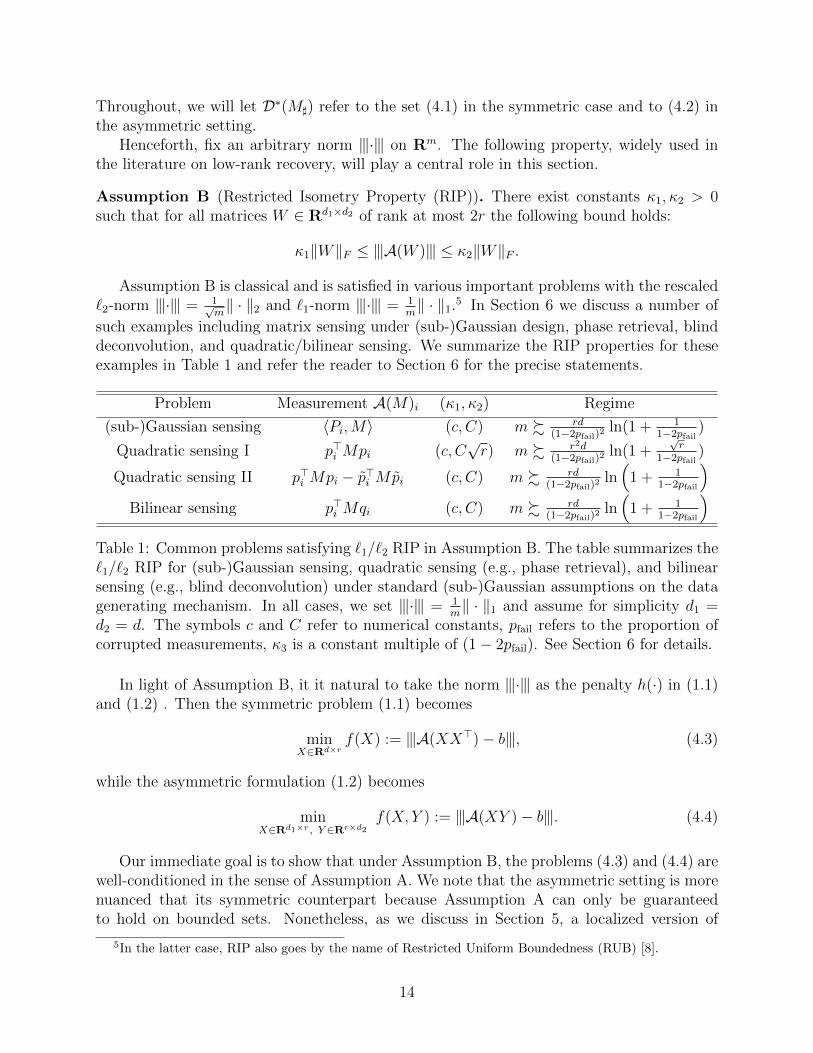
Assumption B (Restricted Isometry Property (RIP)). There exist constants κ1, κ2 > 0such that for all matrices W ∈ Rd1×d2 of rank at most 2r the following bound holds:

κ1‖W‖F ≤ |||A(W )||| ≤ κ2‖W‖F .

Assumption B is classical and is satisfied in various important problems with the rescaled`2-norm |||·||| = 1√

m‖ · ‖2 and `1-norm |||·||| = 1

m‖ · ‖1.5 In Section 6 we discuss a number of

such examples including matrix sensing under (sub-)Gaussian design, phase retrieval, blinddeconvolution, and quadratic/bilinear sensing. We summarize the RIP properties for theseexamples in Table 1 and refer the reader to Section 6 for the precise statements.

Problem Measurement A(M)i (κ1, κ2) Regime

(sub-)Gaussian sensing 〈Pi,M〉 (c, C) m % rd(1−2pfail)2

ln(1 + 11−2pfail

)

Quadratic sensing I p>i Mpi (c, C√r) m % r2d

(1−2pfail)2ln(1 +

√r

1−2pfail)

Quadratic sensing II p>i Mpi − p>i Mpi (c, C) m % rd(1−2pfail)2

ln(

1 + 11−2pfail

)Bilinear sensing p>i Mqi (c, C) m % rd

(1−2pfail)2ln(

1 + 11−2pfail

)Table 1: Common problems satisfying `1/`2 RIP in Assumption B. The table summarizes the`1/`2 RIP for (sub-)Gaussian sensing, quadratic sensing (e.g., phase retrieval), and bilinearsensing (e.g., blind deconvolution) under standard (sub-)Gaussian assumptions on the datagenerating mechanism. In all cases, we set |||·||| = 1

m‖ · ‖1 and assume for simplicity d1 =

d2 = d. The symbols c and C refer to numerical constants, pfail refers to the proportion ofcorrupted measurements, κ3 is a constant multiple of (1− 2pfail). See Section 6 for details.

In light of Assumption B, it it natural to take the norm |||·||| as the penalty h(·) in (1.1)and (1.2) . Then the symmetric problem (1.1) becomes

minX∈Rd×r

f(X) := |||A(XX>)− b|||, (4.3)

while the asymmetric formulation (1.2) becomes

minX∈Rd1×r, Y ∈Rr×d2

f(X, Y ) := |||A(XY )− b|||. (4.4)

Our immediate goal is to show that under Assumption B, the problems (4.3) and (4.4) arewell-conditioned in the sense of Assumption A. We note that the asymmetric setting is morenuanced that its symmetric counterpart because Assumption A can only be guaranteedto hold on bounded sets. Nonetheless, as we discuss in Section 5, a localized version of

5In the latter case, RIP also goes by the name of Restricted Uniform Boundedness (RUB) [8].

14

Assumption A suffices to guarantee rapid local convergence of subgradient and prox-linearmethods. In particular, our analysis of the local sharpness in the asymmetric setting is newand illuminating; it shows that the regularization technique suggested in [39] is not neededat all for the prox-linear method. This conclusion contrasts with known techniques in thesmooth setting, where regularization is often used.

4.1 Approximation and Lipschitz continuity

We begin with the following elementary proposition, which estimates the subgradient boundL and the approximation modulus ρ in the symmetric setting. In what follows, we will usethe expressions

fX(Z) = |||A(XX> +X(Z −X)> + (Z −X)X>)− b|||,f(X,Y )(X, Y ) = |||A(XY +X(Y − Y ) + (X −X)Y )− b|||.

Proposition 4.1 (Approximation accuracy and Lipschitz continuity (symmetric)).Suppose Assumption B holds. Then for all X,Z ∈ Rd×r the following estimates hold:

|f(Z)− fX(Z)| ≤ κ2‖Z −X‖2F ,

|f(X)− f(Z)| ≤ κ2‖X + Z‖op‖X − Z‖F .

Proof. To see the first estimate, observe that

|f(Z)− fX(Z)| = |||A(ZZ>)− b||| − |||A(XX> +X(Z −X)> + (Z −X)X>)− b|||≤ |||A(ZZ> −XX> −X(Z −X)> − (Z −X)X>||| (4.5)

= |||A((Z −X)(Z −X)>

)|||

≤ κ2

∥∥(Z −X)(Z −X)>∥∥F

(4.6)

≤ κ2‖Z −X‖2F ,

where (4.5) follows from the reverse triangle inequality and (4.6) uses Assumption B. Next,for any X,Z ∈ X we successively compute:

|f(X)− f(Z)| =∣∣|||A(XX>)− b||| − |||A(ZZ>)− b|||

∣∣≤∣∣∣∣∣∣A(XX> − ZZ>)

∣∣∣∣∣∣ (4.7)

≤ κ2‖XX> − ZZ>‖F (4.8)

=κ2

2‖(X + Z)(X − Z)> + (X − Z)(X + Z)>‖F

≤ κ2‖(X + Z)(X − Z)‖F≤ κ2‖X + Z‖op‖X − Z‖F ,

where (4.7) follows from the reverse triangle inequality and (4.8) uses Assumption B. Theproof is complete.

The estimates of L and ρ in the asymmetric setting are completely analogous; we recordthem in the following proposition.

15

Proposition 4.2 (Approximation accuracy and Lipschitz continuity (asymmetric)).

Suppose Assumption B holds. Then for all X, X ∈ Rd1×r and Y, Y ∈ Rr×d2 the followingestimates hold:

|f(X, Y )− f(X,Y )(X, Y )| ≤ κ2

2· ‖(X, Y )− (X, Y )‖2

F ,

|f(X, Y )− f(X, Y )| ≤ κ2 max‖X+X‖op,‖Y+Y ‖op√2

· ‖(X, Y )− (X, Y )‖F .Proof. To see the first estimate, observe that

|f(X, Y )− f(X,Y )(X, Y )| =∣∣∣|||A(XY )− b||| − |||A(XY +X(Y − Y ) + (X −X)Y )− b|||

∣∣∣≤ |||A(XY −XY −X(Y − Y )− (X −X)Y )|||= |||A

((X − X)(Y − Y )

)|||

≤ κ2

∥∥∥(X − X)(Y − Y )∥∥∥F

≤ κ2

2

(‖X − X‖2

F + ‖Y − Y ‖2F

),

where the last estimate follows from Young’s inequality 2ab ≤ a2 + b2. Next, we successivelycompute:

|f(X, Y )− f(X, Y )| ≤ |||A(XY − XY )||| ≤ κ2‖XY − XY ‖F=κ2

2‖(X + X)(Y − Y )> + (X − X)(Y + Y )>‖F

≤ κ2 max‖X + X‖op, ‖Y + Y ‖op2

(‖Y − Y ‖F + ‖X − X‖F ).

The result follows by noting that a+ b ≤√

2(a2 + b2) for all a, b ∈ R.

4.2 Sharpness

We next move on to estimates of the sharpness constant µ. We first deal with the noise-less setting b = A(M]) in Section 4.2.1, and then move on to the general case when themeasurements are corrupted by outliers in Section 4.2.2.

4.2.1 Sharpness in the noiseless regime

We begin with with the symmetric setting in the noiseless case b = A(M]). By Assumption B,we have the estimate

f(X) = |||A(XX>)− b||| = |||A(XX> −X]X>] )||| ≥ κ1‖XX> −X]X

>] ‖F . (4.9)

It follows that the set of minimizers argminX∈Rd×r f(X) coincides with the set of minimizersof the function X 7→ ‖XX> −X]X

>] ‖F , namely

D∗(M]) := X]R : R ∈ O(r).Thus to argue sharpness of f it suffices to estimate the sharpness constant of the functionX 7→ ‖XX> −X]X

>] ‖F . Fortunately, this calculation was already done in [57, Lemma 5.4].

16

Proposition 4.3 ([57, Lemma 5.4]). For any matrices X,Z ∈ Rd×r, we have the bound

‖XX> − ZZ>‖F ≥√

2(√

2− 1)σr(Z) · minR∈O(r)

‖X − ZR‖F .

Consequently if Assumption B holds in the noiseless setting b = A(M]), then the bound holds:

f(X) ≥ κ1

√2(√

2− 1)σr(M]) · dist(X,D∗(M])) for all X ∈ Rd×r.

We next consider the asymmetric case. By exactly the same reasoning as before, theset of minimizers of f(X, Y ) coincides with the set of minimizers of the function (X, Y ) 7→‖XY −X]Y]‖F , namely

D∗(M]) := (X]A,A−1Y]) : A ∈ GL(r).

Thus to argue sharpness of f it suffices to estimate the sharpness constant of the function(X, Y ) 7→ ‖XY − X]Y]‖F . Such a sharpness guarantee in the rank one case was recentlyshown in [16, Proposition 4.2].

Proposition 4.4 ([16, Proposition 4.2]). Fix a rank 1 matrix M] ∈ Rd1×d2 and a constantν ≥ 1. Then for any x ∈ Rd1 and w ∈ Rd2 satisfying

‖w‖2, ‖x‖2 ≤ ν√σ1(M]),

the following estimate holds:

‖xw> −M]‖F ≥√σ1(M])

2√

2(ν + 1)· dist

((x,w),D∗(M])

).

Notice that in contrast to the symmetric setting, the sharpness estimate is only valid onbounded sets. Indeed, this is unavoidable even in the setting d1 = d2 = 2. To see this, defineM] = e2e

>2 and for any α > 0 set x = αe1 and w = 1

αe1. It is routine to compute

‖xw> −M]‖Fdist((x,w),D∗(M]))

=

√2

2 + α2 + 1α2

.

Therefore letting α tend to zero (or infinity) the quotient tends to zero.The following corollary is a higher rank extension of Proposition 4.4.

Theorem 4.5 (Sharpness (asymmetric and noiseless)). Fix a constant ν > 0 and defineX] := U

√Λ and Y] =

√ΛV >, where M] = UΛV > is any compact singular value decomposi-

tion of M]. Then for all X ∈ Rd1×r and Y ∈ Rr×d2 satisfying

max‖X −X]‖F , ‖Y − Y]‖F ≤ ν√σr(M])

dist((X, Y ),D∗(M])) ≤√σr(M])

1 + 2(1 +√

2)ν

, (4.10)

the estimate holds:

‖XY −M]‖F ≥√σr(M])

2 + 4(1 +√

2)ν· dist((X, Y ),D∗(M])).

17

Proof. Define δ := 11+2(1+

√2)ν

and consider a pair of matrices X and Y satisfying (4.10). Let

A ∈ GL(r) be an invertible matrix satisfying

A ∈ argminA∈GL(r)

‖X −X]A‖2

F + ‖Y − A−1Y]‖2F

. (4.11)

As a first step, we successively compute

‖XY −X]Y]‖F= ‖(X −X]A)(A−1Y]) +X]A(Y − A−1Y]) + (X −X]A)(Y − A−1Y])‖F≥ ‖(X −X]A)(A−1Y]) +X]A(Y − A−1Y])‖F − ‖(X −X]A)(Y − A−1Y])‖F≥ ‖(X −X]A)(A−1Y]) +X]A(Y − A−1Y])‖F − ‖X −X]A‖F · ‖Y − A−1Y]‖F≥ ‖(X −X]A)(A−1Y]) +X]A(Y − A−1Y])‖F −

1

2(‖X −X]A‖2

F + ‖Y − A−1Y]‖2F )

= ‖(X −X]A)(A−1Y]) +X]A(Y − A−1Y])‖F −1

2dist2((X, Y ),D∗(M]))

≥ ‖(X −X]A)(A−1Y]) +X]A(Y − A−1Y])‖F −δ√σr(M])

2· dist((X, Y ),D∗(M])).

(4.12)

We next aim to lower bound the first term on the right. To this end, observe

‖(X −X]A)(A−1Y]) +X]A(Y − A−1Y])‖2F

= ‖(X −X]A)(A−1Y])‖2F + ‖X]A(Y − A−1Y])‖2

F

+ 2Tr((X −X]A)(A−1Y])(Y − A−1Y])>(X]A)>).

(4.13)

We claim that the cross-term is non-negative. To see this, observe that first order optimalityconditions in (4.11) directly imply that A satisfies the equality

A>X>] (X −X]A) = (Y − A−1Y])Y>] A

−>.

Thus we obtain

Tr((X −X]A)(A−1Y])(Y − A−1Y])>(X]A)>) = Tr(A>X>] (X −X]A)(A−1Y])(Y − A−1Y])

>)

= Tr((Y − A−1Y])Y>] A

−T (A−1Y])(Y − A−1Y])>)

= ‖(A−1Y])(Y − A−1Y])‖2F .

Therefore, returning to (4.13) we conclude that

‖(X −X]A)(A−1Y]) +X]A(Y − A−1Y])‖F≥√‖(X −X]A)(A−1Y])‖2

F + ‖X]A(Y − A−1Y])‖2F

≥√σr(M]) ·minσr(A−1), σr(A) · dist((X, Y ),D∗(M])).

(4.14)

Combining (4.12) and (4.14), we obtain

‖XY −M]‖F ≥√σr(M]) ·

(minσr(A−1), σr(A) − δ

2

)· dist((X, Y ),D∗(M])) (4.15)

18

Finally, we estimate minσr(A−1), σr(A). To this end, first note that

‖X] −X]A‖F + ‖Y] − A−1Y]‖F ≤ ‖X] −X‖F + ‖Y] − Y ‖F +√

2 · dist((X, Y ),D∗(M]))

≤ 2ν√σr(M]) · (1 +

√2).

(4.16)We now aim to lower bound the left-hand-side in terms of minσr(A−1), σr(A). Observe

‖X] −X]A‖F ≥ ‖X] −X]A‖op ≥√σr(M]) · ‖I − A‖op ≥

√σr(M]) · (σ1(A)− 1).

Similarly, we have

‖Y] − A−1Y]‖F ≥ ‖Y] − A−1Y]‖op ≥√σr(M]) · ‖I − A−1‖op ≥

√σr(M]) · (σ1(A−1)− 1).

Hence using (4.16), we obtain the estimate

minσr(A−1), σr(A) ≥(

1 + 2ν · (1 +√

2))−1

= δ.

Using this estimate in (4.15) completes the proof.

4.2.2 Sharpness in presence of outliers

The most important example of the norm |||·||| for us is the scaled `1-norm |||·||| = 1m‖ · ‖1.

Indeed, all the examples in the forthcoming Section 6 will satisfy RIP relative to this norm.In this section, we will show that the `1-norm has an added advantage. Under reasonableRIP-type conditions, sharpness will hold even if up to a half of the measurements are grosslycorrupted.

Henceforth, for any set I, define the restricted map AI := (A(X))i∈I . We interpretthe set I as corresponding to (arbitrarily) outlying measurements, while its complementcorresponds to exact measurements. Motivated by the work [27] on robust phase retrieval,we make the following assumption.

Assumption C (I-outlier bounds). There exists a set I ⊂ 1, . . . ,m and a constant κ3 > 0such that the following hold.

(C1) Equality holds bi = A(M])i for all i /∈ I.

(C2) For all matrices W of rank at most 2r, we have

κ3‖W‖F ≤1

m‖AIc(W )‖1 −

1

m‖AI(W )‖1. (4.17)

The assumption is simple to interpret. To elucidate the bound (4.17), let us suppose thatthe restricted maps AI and AIc satisfy Assumption B (RIP) with constants κ1, κ2 and κ1,κ2, respectively. Then for any rank 2r matrix X we immediately deduce the estimate

1

m‖AIc(W )‖1 −

1

m‖AI(W )‖1 ≥ ((1− pfail)κ1 − pfailκ2) ‖W‖F ,

19

where pfail = |I|m

denotes the corruption frequency. In particular, the right-hand side ispositive as long as the corruption frequency is below the threshold pfail <

κ1κ1+κ2

.Combining Assumption C with Proposition 4.3 quickly yields sharpness of the objective

even in the noisy setting.

Proposition 4.6 (Sharpness with outliers (symmetric)). Suppose that Assumption C holds.Then

f(X)− f(X]) ≥ κ3

(√2(√

2− 1)σr(X])

)dist(X,D∗(M])

)for all X ∈ Rd×r.

Proof. Defining ∆ := A(X]X>] )− b, we have the following bound:

m · (f(X)− f(X])) = ‖A(XX> −X]X

>]

)+ ∆‖1 − ‖∆‖1

= ‖AIc(XX> −X]X>] )‖1 +

∑i∈I

(|(A(XX> −X]X

>] ))i+ ∆i| − |∆i|

)≥ ‖AIc(XX> −X]X

>] )‖1 − ‖AI(XX> −X]X

>] )‖1

≥ κ3m‖XX> −X]X>] ‖F ≥ κ3m

(√2(√

2− 1)σr(X])

)dist(X,D∗(M])

),

where the first inequality follows by the reverse triangle inequality, the second inequalityfollows by Assumption (C2), and the final inequality follows from Proposition 4.3. Theproof is complete.

The argument in the asymmetric setting is completely analogous.

Proposition 4.7 (Sharpness with outliers (asymmetric)). Suppose that Assumption C holds.Fix a constant ν > 0 and define X] := U

√Λ and Y] =

√ΛV >, where M] = UΛV > is any

compact singular value decomposition of M]. Then for all X ∈ Rd1×r and Y ∈ Rr×d2

satisfying

max‖X −X]‖F , ‖Y − Y]‖F ≤ ν√σr(M])

dist((X, Y ),D∗(M])) ≤√σr(M])

1 + 2(1 +√

2)ν

The estimate holds:

f(X, Y )− f(X], Y]) ≥κ3

√σr(M])

2 + 4(1 +√

2)ν· dist((X, Y ),D∗(M])).

5 General convergence guarantees for subgradient &

prox-linear methods

In this section, we formally develop convergence guarantees for Algorithms 1, 2, and 3 underAssumption A, and deduce performance guarantees in the RIP setting. To this end, it will be

20

useful to first consider a broader class than the compositional problems (3.1). We say that afunction f : E→ R∪+∞ is ρ-weakly convex6 if the perturbed function x 7→ f(x)+ ρ

2‖x‖2

2 isconvex. In particular, a composite function f = hF satisfying the approximation guarantee

|fx(y)− f(y)| ≤ ρ

2‖y − x‖2

2 ∀x, y

is automatically ρ-weakly convex [26, Lemma 4.2]. Subgradients of weakly convex functionsare very well-behaved. Indeed, notice that in general the little-o term in the expression (2.1)may depend on the basepoint x, and may therefore be nonuniform. The subgradients ofweakly convex functions, on the other hand, automatically satisfy a uniform type of lower-approximation property. Indeed, a lower-semicontinuous function f is ρ-weakly convex ifand only if it satisfies:

f(y) ≥ f(x) + 〈ξ, y − x〉 − ρ

2‖y − x‖2

2 ∀x, y ∈ E, ξ ∈ ∂f(x).

Setting the stage, we introduce the following assumption.

Assumption D. Consider the optimization problem,

minx∈X

f(x). (5.1)

Suppose that the following properties hold for some real numbers µ, ρ > 0.

1. (Weak convexity) The set X is closed and convex, while the function f : E → R isρ-weakly convex.

2. (Sharpness) The set of minimizers X ∗ := argminx∈X

f(x) is nonempty and the following

inequality holds:f(x)− inf

Xf ≥ µ · dist (x,X ∗) ∀x ∈ X .

In particular, notice that Assumption A implies Assumption D. Taken together, weakconvexity and sharpness provide an appealing framework for deriving local rapid conver-gence guarantees for numerical methods. In this section, we specifically focus on two suchprocedures: the subgradient and prox-linear algorithms. We aim to estimate both the radiusof rapid converge around the solution set and the rate of convergence. Note that both ofthe algorithms, when initialized at a stationary point could stay there for all subsequentiterations. Since we are interested in finding global minima, we therefore estimate the neigh-borhood of the solution set that has no extraneous stationary points. This is the content ofthe following simple lemma.

Lemma 5.1 ([23, Lemma 3.1]). Suppose that Assumption D holds. Then the problem (5.1)has no stationary points x satisfying

0 < dist(x;X ∗) < 2µ

ρ.

6Weakly convex functions also go by other names such as lower-C2, uniformly prox-regularity, paraconvex,and semiconvex. We refer the reader to the seminal works on the topic [2, 47,49,51,53].

21

It is worthwhile to note that the estimate 2µρ

of the radius in Lemma 5.1 is tight [16,

Section 3]. Hence, let us define for any γ > 0 the tube

Tγ :=

z ∈ X : dist(z,X ∗) ≤ γ · µ

ρ

. (5.2)

Thus we would like to search for algorithms whose basin of attraction is a tube Tγ for somenumerical constant γ > 0. Such a basin of attraction is in essence optimal.

The rate of convergence of the subgradient methods (Algorithms 1 and 2) relies on thesubgradient bound and the condition measure:

L := sup‖ζ‖2 : ζ ∈ ∂f(x), x ∈ T1 and τ :=µ

L.

A straightforward argument [23, Lemma 3.2] shows τ ∈ [0, 1]. The following theorem appearsas [23, Theorem 4.1], while its application to phase retrieval was investigated in [24].

Theorem 5.2 (Polyak subgradient method). Suppose that Assumption D holds and fix areal number γ ∈ (0, 1). Then Algorithm 1 initialized at any point x0 ∈ Tγ produces iteratesthat converge Q-linearly to X ∗, that is

dist2(xk+1,X ∗) ≤(1− (1− γ)τ 2

)dist2(xk,X ∗) ∀k ≥ 0.

The following theorem appears as [23, Theorem 6.1]. The convex version of the resultdates back to Goffin [34].

Theorem 5.3 (Geometrically decaying subgradient method). Suppose that Assumption D

holds, fix a real number γ ∈ (0, 1), and suppose τ ≤√

12−γ . Set λ := γµ2

ρLand q :=√

1− (1− γ)τ 2 in Algorithm 2. Then the iterates xk generated by Algorithm 2, initializedat any point x0 ∈ Tγ, satisfy:

dist2(xk;X ∗) ≤γ2µ2

ρ2

(1− (1− γ)τ 2

)k ∀k ≥ 0.

Let us now specialize to the composite setting under Assumption A. Since Assumption Aimplies Assumption D, both subgradient Algorithms 1 and 2 will enjoy a linear rate ofconvergence when initialized sufficiently close the solution set. The following theorem, onthe other hand, shows that the prox-linear method will enjoy a quadratic rate of convergence(at the price of a higher per-iteration cost). Guarantees of this type have appeared, forexample, in [7, 25,27].

Theorem 5.4 (Prox-linear algorithm). Suppose Assumption A holds. Choose any β ≥ ρ inAlgorithm 3 and set γ := ρ/β. Then Algorithm 3 initialized at any point x0 ∈ Tγ convergesquadratically:

dist(xk+1,X ∗) ≤ βµ· dist2(xk,X ∗) ∀k ≥ 0.

We now apply the results above to the low-rank matrix factorization problem under RIP,whose regularity properties were verified in Section 4. In particular, we have the followingefficiency guarantees of the subgradient and prox-linear methods applied to this problem.

22

Corollary 5.5 (Convergence guarantees under RIP (symmetric)). Suppose Assumptions Band C are valid with |||·||| = 1

m‖ · ‖1 and consider the optimization problem

minX∈Rd×r

f(X) =1

m‖A(XX>)− b‖1.

Choose any matrix X0 satisfying

dist(X0,D∗(M]))√σr(M])

≤ 0.2 · κ3

κ2

.

Define the condition number χ := σ1(M])/σr(M]). Then the following are true.

1. (Polyak subgradient) Algorithm 1 initialized at X0 produces iterates that convergelinearly to D∗(M]), that is

dist2(Xk,D∗(M]))

σr(M])≤

1− 0.2

1 +4κ22χ

κ23

k

· κ23

100κ22

∀k ≥ 0.

2. (geometric subgradient) Algorithm 2 with λ =0.81κ23

√σr(M])

2κ2(κ3+2κ2√χ)

, q =√

1− 0.21+4κ22χ/κ

23

and initialized at X0 converges linearly:

dist2(Xk,D∗(M]))

σr(M])≤

1− 0.2

1 +4κ22χ

κ23

k

· κ23

100κ22

∀k ≥ 0.

3. (prox-linear) Algorithm 3 with β = ρ and initialized at X0 converges quadratically:

dist(Xk,D∗(M])))√σr(M])

≤ 2−2k · 0.45κ3

κ2

∀k ≥ 0.

5.1 Guarantees under local regularity

As explained in Section 4, Assumptions A and D are reasonable in the symmetric settingunder RIP. The asymmetric setting is more nuanced. Indeed, the solution set is unbounded,while uniform bounds on the sharpness and subgradient norms are only valid on boundedsets. One remedy, discussed in [39], is to modify the optimization formulation by introducinga form of regularization:

minX,Y|||A(XY )− y|||+ λ‖X>X − Y Y >‖F .

In this section, we take a different approach that requires no modification to the optimizationproblem nor the algorithms. The key idea is to show that if the problem is well-conditionedonly on a neighborhood of a particular solution, then the iterates will remain in the neighbor-hood provided the initial point is sufficiently close to the solution. In fact, we will see that theiterates themselves must converge. The proofs of the results in this section (Theorems 5.6,5.7, and 5.8) are deferred to Appendix A.

We begin with the following localized version of Assumption D.

23

Assumption E. Consider the optimization problem,

minx∈X

f(x). (5.3)

Fix an arbitrary point x ∈ X ∗ and suppose that the following properties hold for some realnumbers ε, µ, ρ > 0.

1. (Local weak convexity) The set X is closed and convex, and the bound holds:

f(y) ≥ f(x) + 〈ζ, y − x〉 − ρ

2‖y − x‖2

2 ∀x, y ∈ X ∩Bε(x), ζ ∈ ∂f(x).

2. (Local sharpness) The inequality holds:

f(x)− infXf ≥ µ · dist (x,X ∗) ∀x ∈ X ∩Bε(x).

The following two theorems establish convergence guarantees of the two subgradientmethods under Assumption E. Abusing notation slightly, we define the local quantities:

L := supζ∈∂f(x)

‖ζ‖2 : x ∈ X ∩Bε(x) and τ :=µ

L.

Theorem 5.6 (Polyak subgradient method (local regularity)). Suppose Assumption E holdsand fix an arbitrary point x0 ∈ Bε/4(x) satisfying

dist(x0,X ∗) ≤ min

3εµ2

64L2,µ

2ρ

.

Then Algorithm 1 initialized at x0 produces iterates xk that always lie in Bε(x) and satisfy

dist2(xk+1,X ∗) ≤(1− 1

2τ 2)

dist2(xk,X ∗), for all k ≥ 0. (5.4)

Moreover the iterates converge to some point x∞ ∈ X ∗ at the R-linear rate

‖xk − x∞‖2 ≤16L3 · dist(x0,X ∗)

3µ3·(1− 1

2τ 2) k

2 for all k ≥ 0.

Theorem 5.7 (Geometrically decaying subgradient method (local regularity)). Suppose that

Assumption E holds and that τ ≤ 1√2. Define γ = ερ

4L+ερ, λ = γµ2

ρL, and q =

√1− (1− γ)τ 2.

Then Algorithm 2 initialized at any point x0 ∈ Bε/4(x)∩Tγ generates iterates xk that alwayslie in Bε(x) and satisfy

dist2(xk;X ∗) ≤γ2µ2

ρ2

(1− (1− γ)τ 2

)kfor all k ≥ 0. (5.5)

Moreover, the iterates converge to some point x∞ ∈ X ∗ at the R-linear rate

‖xk − x∞‖2 ≤ λ1−q · qk for all k ≥ 0.

24

We end the section by specializing to the composite setting and analyzing the prox-linearmethod. The following is the localized version of Assumption A.

Assumption F. Consider the optimization problem,

minx∈X

f(x) := h(F (x)),

where the function h(·) and the set X are convex and F (·) is differentiable. Fix a pointx ∈ X ∗ and suppose that the following properties holds for some real numbers ε, µ, ρ > 0.

1. (Approximation accuracy) The convex models fx(y) := h(F (x) + ∇F (x)(y − x))satisfy the estimate:

|f(y)− fx(y)| ≤ ρ

2‖y − x‖2

2 ∀x ∈ X ∩Bε(x), y ∈ X .

2. (Sharpness) The inequality holds:

f(x)− infXf ≥ µ · dist (x,X ∗) ∀x ∈ X ∩Bε(x).

The following theorem provides convergence guarantees for the prox-linear method underAssumption F.

Theorem 5.8 (Prox-linear (local)). Suppose Assumption F holds, choose any β ≥ ρ, andfix an arbitrary point x0 ∈ Bε/2(x) satisfying

f(x0)−minX

f ≤ min

βε2

25,µ2

2β

.

Then Algorithm 3 initialized at x0 generates iterates xk that always lie in Bε(x) and satisfy

dist(xk+1,X ∗) ≤β

µ· dist2(xk,X ∗),

f(xk+1)−minX

f ≤ β

µ2

(f(xk)−min

Xf)2

.

Moreover the iterates converge to some point x∞ ∈ X ∗ at the quadratic rate

‖xk − x∞‖2 ≤2√

2µ

β·(

1

2

)2k−1

for all k ≥ 0.

With the above generic results in hand, we can now derive the convergence guarantees forthe subgradient and prox-linear methods for asymmetric low-rank matrix recovery problems.To summarize, the prox-linear method converges quadratically, as long as it is initializedwithin constant relative error of the solution. The guarantees for the subgradient methodsare less satisfactory: the size of the region of the linear convergence scales with the conditionnumber of M]. The reason is that the proof estimates the region of convergence using thelength of the iterate path, which scales with the condition number. The dependence onthe condition number in general can be eliminated by introducing regularization ‖X>X −Y Y >‖F , as suggested in the work [39]. Still the results we present here are notable evenfor the subgradient method. For example, we see that for rank r = 1 instances satisfyingRIP (e.g. blind deconvolution), the condition number of M] is always one and thereforeregularization is not required at all for subgradient and prox-linear methods.

25

Corollary 5.9 (Convergence guarantees under RIP (asymmetric)). Suppose Assumptions Band C are valid7 and consider the optimization problem

minX∈Rd1×r, Y ∈Rr×d2

f(X) =1

m‖A(XY )− b‖1.

Define X] := U√

Λ and Y] =√

ΛV >, where M] = UΛV > is any compact singular valuedecomposition of M]. Define also the condition number χ := σ1(M])/σr(M]). Then thereexists η > 0 depending only on κ2, κ3, and σ(M]) such that the following are true.

1. (Polyak subgradient) Algorithm 1 initialized at (X0, Y0) satisfying‖(X0,Y0)−(X],Y])‖F√

σr(M]).

min1, κ23κ22χ

, κ3κ2, will generate an iterate sequence that converges at the linear rate:

dist((Xk, Yk),D∗(M]))√σr(M])

≤ δ after k &κ2

2χ2

κ23

· ln(ηδ

)iterations.

2. (geometric subgradient) Algorithm 2 initialized at (X0, Y0) satisfying‖(X0,Y0)−(X],Y])‖F√

σr(M]).

min1, κ3κ2χ, will generate an iterate sequence that converges at the linear rate:

dist((Xk, Yk),D∗(M]))√σr(M])

≤ δ after k &κ2

2χ2

κ23

· ln(ηδ

)iterations.

3. (prox-linear) Algorithm 3 initialized at (X0, Y0) satisfying f(x0)−minX fσr(M])

. minκ2, κ23/κ2

and‖(X0,Y0)−(X],Y])‖F√

σr(M]). 1, will generate an iterate sequence that converges at the

quadratic rate:

dist((Xk, Yk),D∗(M]))√σr(M])

.κ3

κ2

· 2−2k for all k ≥ 0.

6 Examples of `1/`2 RIP

In this section, we survey three matrix recovery problems from different fields, includingphysics, signal processing, control theory, wireless communications, and machine learning,among others. In all cases, the problems satisfy `1/`2 RIP and the I-outlier bounds andconsequently, the convergence results in Corollaries 5.5 and 5.9 immediately apply. Most ofthe RIP results in this section were previously known (albeit under more restrictive assump-tions); we provide self-contained arguments in the Appendix B for the sake of completeness.On the other hand, using nonsmooth optimization in these problems and the correspondingconvergence guarantees based on RIP are, for the most part, new.

For the rest of this section we will assume the following data-generating mechanism.

7 with |||·||| = 1m‖ · ‖1

26

Definition 6.1 (Data-generating mechanism). A random linear map A : Rd1×d2 → Rm

and a random index set I ⊂ [m] are drawn independently of each other. We assume moreoverthat the outlier frequency pfail := |I|/m satisfies pfail ∈ [0, 1/2) almost surely. We thenobserve the corrupted measurements

bi =

A(M]) if i /∈ I, and

ηi if i ∈ I, (6.1)

where η is an arbitrary vector. In particular, η could be correlated with A.

Throughout this section, we consider four distinct linear operators A.

Matrix Sensing. In this scenario, measurements are generated as follows:

A(M])i := 〈Pi,M]〉 for i = 1, . . . ,m (6.2)

where Pi ∈ Rd1×d2 are fixed matrices.

Quadratic Sensing I . In this scenario, M] ∈ Rd×d is assumed to be a PSD rank r matrixwith factorization M] = X]X

>] and measurements are generated as follows:

A(M])i = p>i M]pi = ‖X>] pi‖22 for i = 1, . . . ,m, (6.3)

where pi ∈ Rd are fixed vectors.

Quadratic Sensing II . In this scenario, M] ∈ Rd×d is assumed to be a PSD rank rmatrix with factorization M] = X]X

>] and measurements are generated as follows:

A(M])i = p>i M]pi − p>i M]pi = ‖X>] pi‖22 − ‖X>] pi‖2

2 for i = 1, . . . ,m, (6.4)

where pi, pi ∈ Rd are fixed vectors.

Bilinear Sensing. In this scenario, M] ∈ Rd1×d2 is assumed to be a r matrix with factor-ization M] = XY and measurements are generated as follows:

A(M])i = p>i M]qi for i = 1, . . . ,m, (6.5)

where pi ∈ Rd1 and qi ∈ Rd2 are fixed vectors.

The matrix, quadratic, and bilinear sensing problems have been considered in a numberof papers and in a variety of applications. The first theoretical properties for matrix sensingwere discussed in [13, 30, 50]. Quadratic sensing in its full generality appeared in [18] andis a higher-rank generalization of the much older (real) phase retrieval problem [10, 14, 35].Besides phase retrieval, quadratic sensing has applications to covariance sketching, shallowneural networks, and quantum state tomography; see for example [40] for a discussion. Bilin-ear sensing is a natural modification of quadratic sensing and is a higher-rank generalizationof the blind deconvolution problem [1]; it was first proposed and studied in [8].

27

The reader is reminded that once `1/`2 RIP guarantees, in particular Assumptions Band C, are established for the above four operators, the guarantees of Corollaries 5.5 andCorollary 5.9 immediately take hold for the problems

minX∈Rd×r

f(X) =1

m‖A(XX>)− b‖1

and

minX∈Rd1×r, Y ∈Rr×d2

f(X) =1

m‖A(XY )− b‖1,

respectively. Thus, we turn our attention to establishing such guarantees.

6.1 Warm-up: `2/`2 RIP for matrix sensing with Gaussian design

In this section, we are primarily interested in the `1/`2 RIP for the above four linear operators.However, as a warm-up, we first consider the `2/`2-RIP property for matrix sensing withGaussian Pi. The following result appears in [13,50].

Theorem 6.2 (`2/`2-RIP for matrix sensing). For any δ ∈ (0, 1) there exist constantsc, C > 0 depending only on δ such that if the entries of Pi are i.i.d. standard Gaussian andm ≥ cr(d1 + d2) log(d1d2), then with probability at least 1− exp (−Cm), the estimate

(1− δ)‖M‖F ≤1√m‖A(M)‖2 ≤ (1 + δ)‖M‖F ,

holds simultaneously for all M ∈ Rd1×d2 of rank at most 2r. Consequently, Assumption B issatisfied.

Following the general recipe of the paper, we see that the nonsmooth formulation

minX∈Rd1×r, Y ∈Rr×d2

1√m‖A(XY )− b‖2 =

√√√√ 1

m

m∑i=1

(Tr(Y P>i X)− bi

)2(6.6)

is immediately amenable to subgradient and prox-linear algorithms in the noiseless settingI = ∅. In particular, a direct analogue of Corollary 5.9, which was stated for the penaltyfunction h = 1

m‖ · ‖1, holds; we omit the straightforward details.

6.2 The `1/`2 RIP and I-outlier bounds: quadratic and bilinearsensing

We now turn our attention to the `1/`2 RIP for more general classes of linear maps than thei.i.d. Gaussian matrices considered in Theorem 6.2. To establish such guarantees, one mustensure that the linear maps A have light tails and are robustly injective on certain spaces ofmatrices. The first property leads to tight concentration results, while the second yields theexistence of a lower RIP constant κ1.

28

Assumption G (Matrix Sensing). The matrices Pi are i.i.d. realizations of an η-sub-Gaussian random matrix8 P ∈ Rd1×d2 . Furthermore, there exists a numerical constant α > 0such that

infM : Rank M≤2r‖M‖F=1

E|〈P,M〉| ≥ α. (6.7)

Assumption H (Quadratic Sensing I). The vectors pi are i.i.d. realizations of a η-sub-Gaussian random variable p ∈ Rd. Furthermore, there exists a numerical constant α > 0such that

infM∈Sd: Rank M≤2r

‖M‖F=1

E|p>Mp| ≥ α. (6.8)

Assumption I (Quadratic Sensing II). The vectors pi, pi are i.i.d. realizations of a η-sub-Gaussian random variable p ∈ Rd. Furthermore, there exists a numerical constant α > 0such that

infM∈Sd: Rank M≤2r

‖M‖F=1

E|p>Mp− p>Mp| ≥ α. (6.9)

Assumption J (Bilinear Sensing). The vectors pi and qi are i.i.d. realizations of η-sub-Gaussian random vectors p ∈ Rd1 and q ∈ Rd2 , respectively. Furthermore, there exists anumerical constant α > 0 such that

infM : Rank M≤2r‖M‖F=1

E|p>Mq| ≥ α. (6.10)

The Assumptions G-J are all valid for i.i.d. Gaussian realizations with independent identitycovariance, as the following lemma shows. We defer its proof to Appendix B.1.

Lemma 6.3. Assumption G holds for matrices P with i.i.d. standard Gaussian entries.Assumptions H and I hold for vectors p, p with i.i.d. standard Gaussian entries. Assumption Jholds for vectors p and q with i.i.d. standard Gaussian entries.

We can now state the main RIP guarantees under the above assumptions. Throughoutall the results, we fix the data generating mechanism as in Definition 6.1. Then, we wish toestablish the inequalities

κ1‖M‖F ≤1

m‖A(M)‖1 ≤ κ2‖M‖F (6.11)

and

κ3‖M‖F ≤1

m

(‖AIc(M)‖1 − ‖AI(M)‖1

), (6.12)

and, hence, Assumptions B and C, respectively, for certain constants κ1, κ2, and κ3. Wedefer the proof of this theorem to Appendix B.2.

Theorem 6.4 (`1/`2 RIP and I-outlier bounds). There exist numerical constants c1, . . . , c6 >0 depending only on α, η such that the following hold for the corresponding measurement op-erators described in Equations (6.2), (6.3), (6.4), and (6.5), respectively

8By this we mean that the vectorized matrix vec(P ) is a η-sub-gaussian random vector.

29

1. (Matrix sensing) Suppose Assumption G holds. Then provided m ≥ c1(1−2pfail)2

r(d1 +

d2 + 1) ln(c2 + c2

1−2pfail

), we have with probability at least 1− 4 exp (−c3(1− 2pfail)

2m)

that every matrix M ∈ Rd1×d2 of rank at most 2r satisfies (6.11) and (6.12) withconstants κ1 = c4, κ2 = c5 and κ3 = c6(1− 2pfail).

2. (Quadratic sensing I) Suppose Assumption H holds. Then provided m ≥ c1(1−2pfail)2

r2(2d+

1) ln(c2 + c2

1−2pfail

√r)

, we have with probability at least 1− 4 exp (−c3(1− 2pfail)2m/r)

that every matrix M ∈ Rd×d of rank at most 2r satisfies (6.11) and (6.12) with con-stants κ1 = c4, κ2 = c5 ·

√r and κ3 = c6(1− 2pfail).

3. (Quadratic sensing II) Suppose Assumption I holds. Then provided m ≥ c1(1−2pfail)2

r(2d+

1) ln(c2 + c2

1−2pfail

), we have with probability at least 1− 4 exp (−c3(1− 2pfail)

2m) that

every matrix M ∈ Rd×d of rank at most 2r satisfies (6.11) and (6.12) with constantsκ1 = c4, κ2 = c5 and κ3 = c6(1− 2pfail).

4. (Bilinear sensing) Suppose Assumption J holds. Then provided m ≥ c1(1−2pfail)2

r(d1 +

d2 + 1) ln(c2 + c2

1−2pfail

), we have with probability at least 1− 4 exp (−c3(1− 2pfail)

2m)

that every matrix M ∈ Rd1×d2 of rank at most 2r satisfies (6.11) and (6.12) withconstants κ1 = c4, κ2 = c5 and κ3 = c6(1− 2pfail).

The guarantees of Theorem 6.4 were previously known under stronger assumptions. Inparticular, item (1) generalizes the results in [39] for the pure Gaussian setting. The caser = 1 of item (2) can be found, in a sightly different form, in [27, 29]. Item (3) sharpensslightly the analogous guarantee in [18] by weakening the assumptions on the moments ofthe measuring vectors to the uniform lower bound (6.9). Special cases of item (4) wereestablished in [16], for the case r = 1, and [8], for Gaussian measurement vectors.

We note that all linear mappings require the same number of measurements in order tosatisfy RIP and I outlier bounds, except for quadratic sensing I operator, which incurs anextra r-factor. This reveals the utility of the quadratic sensing II operator, which achievesoptimal sample complexity. For larger scale problems, a shortcoming of matrix sensingoperator (6.2) is that md1d2 scalars are required to represent the map A. In contrast, allother measurement operators may be represented with only m(d1 + d2) scalars.

7 Matrix Completion

In the previous sections, we saw that low-rank recovery problems satisfying RIP lead towell-conditioned nonsmooth formulations. We claim, however, that the general frameworkof sharpness and approximation is applicable even for problems without RIP. We considertwo such problems, namely matrix completion in this section and robust PCA in Section 8,to follow. Both problems will be considered in the symmetric setting.

The goal of matrix completion problem is to recover a PSD rank r matrix M] ∈ Sd givenaccess only to a subset of its entries. Henceforth, let X] ∈ Rd×r be a matrix satisfyingM] = X]X

>] . Throughout, we assume incoherence condition, ‖X]‖2,∞ ≤

√νrd

, for some

30

ν > 0. We also make the fairly strong assumption that the singular values of X] are allequal σ1(X]) = σ2(X]) = . . . = σr(X]) = 1. This assumption is needed for our theoreticalresults. We let Ω ⊆ [d] × [d] be an index set generated by the Bernoulli model, that is,P((i, j), (j, i) ∈ Ω) = p independently for all 1 ≤ i ≤ j ≤ d. Let ΠΩ : Sd → R|Ω| be theprojection onto the entries indexed by Ω. We consider the following optimization formulationof the problem

minX∈X

f(X) = ‖ΠΩ(XX>)− ΠΩ(M])‖2 where X =

X ∈ Rd×r : ‖X‖2,∞ ≤

√νr

d

.

We will show that both the Polyak subgradient method and an appropriately modified prox-linear algorithm converge linearly to the solution set under reasonable initialization. More-over, we will see that the linear rate of convergence for the prox-linear method is much betterthan that for the subgradient method.

To simplify notation, we set

D∗ := D∗(M]) = X ∈ Rd1×r : XX> = M].

We begin by estimating the sharpness constant µ of the objective function. Fortunately,this estimate follows directly from inequalities (58) and (59a) in [19].

Lemma 7.1 (Sharpness [19]). There are numerical constant c1, c2 > 0 such that the followingholds. If p ≥ c2(ν

2r2

d+ log d

d), then with probability 1− c1d

−2, the estimate

1

p‖ΠΩ(XX> −X]X

>] )‖2

F ≥ c1‖XX> −X]X>] ‖2

F

holds uniformly for all X ∈ X with dist(X,D∗) ≤ c1.

Let us next estimate the approximation accuracy |f(Z)− fX(Z)|, where

fX(Z) = ‖ΠΩ(XX −M] +X(Z −X)> + (Z −X)X>)‖F .

To this end, we will require the following result.

Lemma 7.2 (Lemma 5 in [19]). There is a numerical constant c > 0 such that the followingholds. If p ≥ c

ε2(ν

2r2

d+ log d

d) for some ε ∈ (0, 1), then with probability at least 1 − 2d−4, the

estimates

1. 1√p‖ΠΩ(HH>)‖F ≤

√(1 + ε)‖H‖2

F +√ε‖H‖F ; and

2. 1√p‖ΠΩ(GH>)‖F ≤

√νr‖G‖F

hold uniformly for all matrices H with ‖H‖2,∞ ≤ 6√

νrd

and G ∈ Rd×r.

An estimate of the approximation error |f(Z)− fX(Z)| is now immediate.

31

Lemma 7.3 (Approximation accuracy and Lipschitz continuity). There is a numerical con-stant c > 0 such that the following holds. If p ≥ c

ε2(ν

2r2

d+ log d

d) for some ε ∈ (0, 1), then with

probability at least 1− 2d−4, the estimates

1√p|f(X)− fY (X)| ≤

√(1 + ε)‖X − Y ‖2

F +√ε‖X − Y ‖F ,

|f(X)− f(Y )| ≤ √pνr‖X − Y ‖F ,

holds uniformly for all X, Y ∈ X .

Proof. The first inequality follows immediately by observing the estimate

|f(X)− fY (X)| ≤ ‖ΠΩ((X − Y )(X − Y )>)‖F ,

and using Lemma 7.2. To see the second inequality, observe

|f(X)− f(Y )| ≤ ‖ΠΩ(XX> − Y Y >)‖F=

1

2‖ΠΩ((X − Y )(X + Y )> − (X + Y )(X − Y )>)‖F

≤ ‖ΠΩ((X − Y )(X + Y )>)‖F≤ √pνr‖X − Y ‖F ,

where the last inequality follows by Part 2 of Lemma 7.2.

Note that the approximation bound in Lemma 7.2 is not in terms of the square Euclideannorm. Therefore the results in Section 5 do not apply directly. Nonetheless, it is straightfor-ward to modify the prox-linear method to take into account the new approximation bound.The proof of the following lemma appears in the appendix.

Lemma 7.4. Suppose that Assumption A holds with the approximation property replaced by

|f(y)− fx(y)| ≤ a‖y − x‖22 + b‖y − x‖2 ∀x, y ∈ X ,

for some real a, b ≥ 0. Consider the iterates generated by the process:

xk+1 = argminx∈X

fxk(x) + a‖x− xk‖2

2 + b‖x− xk‖2

.

Then as long as x0 satisfies dist(x0,X ∗) ≤ µ−2b2a

, the iterates converge linearly:

dist(xk+1,X ∗) ≤2(b+ adist(x,X ∗))

µ· dist(xk,X ∗) ∀k ≥ 0.

Combining Lemma 7.4 with our estimates of the sharpness and approximation accuracy,we deduce the following convergence guarantee for matrix completion.

32

Corollary 7.5 (Prox-linear method for matrix completion). There are numerical constantsc0, c, C > 0 such that the following holds. If p ≥ c

ε2(ν

2r2

d+ log d

d) for some ε ∈ (0, 1), then with

probability at least 1− c0d−2, the iterates generated by the modified prox-linear algorithm

Xk+1 = argminX∈X

fXk(X) +

√p(1 + ε) · ‖X −Xk‖2

2 +√pε‖X −Xk‖2

(7.1)

satisfy

dist(Xk+1,D∗) ≤√ε+√

1 + ε · dist(Xk,D∗)C

· dist(Xk,D∗) ∀k ≥ 0.

In particular, the iterates converge linearly as long as dist(X0,D∗) < C−2√ε

2√

(1+ε).

Proof. By invoking Proposition 4.3 and Lemmas 7.1 and 7.3 we may appeal to Lemma 7.4

with a =√p(1 + ε), b =

√pε, and µ =

√2c1p(

√2− 1). The result follows immediately.

To summarize, there exist numerical constants c0, c1, c2, c3 > 0 such that the following istrue with probability at least 1− c0d

−2. In the regime

p ≥ c2

ε2

(ν2r2

d+

log d

d

)for some ε ∈ (0, c1),

the prox-linear method will converge at the rapid linear rate,

dist(Xk,D∗) ≤c2

2k,

when initialized at X0 ∈ X satisfying dist(X0,D∗) < c2.As for the prox-linear method, the results of Section 5 do not immediately yield con-

vergence guarantees for the Polyak subgradient method. Nonetheless, it straightforward toshow that the standard Polyak subgradient method still enjoys local linear convergence guar-antees. The proof is a straightforward modification of the argument in [23, Theorem 3.1],and appears in the appendix.

Theorem 7.6. Suppose that Assumption A holds with the approximation property replacedby

|f(y)− fx(y)| ≤ a‖y − x‖22 + b‖y − x‖2 ∀x, y ∈ X ,

for some real a, b ≥ 0. Consider the iterates xk generated by the Polyak subgradientmethod in Algorithm 1. Then as long as the sharpness constant satisfies µ > 2b and x0

satisfies dist(x0,X ∗) ≤ γ · µ−2b2a

for some γ < 1, the iterates converge linearly

dist2(xk+1,X ∗) ≤(

1− (1− γ)µ(µ− 2b)

L2

)· dist2(xk,X ∗) ∀k ≥ 0.

Finally, combining Theorem 7.6 with our estimates of the sharpness and approximationaccuracy, we deduce the following convergence guarantee for matrix completion.

33

Corollary 7.7 (Subgradient method for matrix completion). There are numerical constantsc0, c, C > 0 such that the following holds. If p ≥ c

ε2(ν

2r2

d+ log d

d) for some ε ∈ (0, 1), then

with probability at least 1 − c0d−2, the iterates generated by the iterates Xk generated by

the Polyak Subgradient method in Algorithm 1 satisfy

dist(Xk+1,D∗)2 ≤(

1− C(C − 2√ε)

2νr

)· dist2(Xk,D∗) ∀k ≥ 0.

In particular, the iterates converge linearly as long as dist(X0,D∗) < C−2√ε

4√

(1+ε).

Proof. First, observe that we have the bound L ≤ √pνr by Lemma 7.3. By invokingProposition 4.3 and Lemmas 7.1 and 7.3 we may appeal to Theorem 7.6 with γ = 1/2,

a =√p(1 + ε), b =

√pε, and µ =

√2c1p(

√2− 1). The result follows immediately.

To summarize, there exist numerical constants c0, c1, c2, c3 > 0 such that the following istrue with probability at least 1− c0d

−2. In the regime

p ≥ c2

ε2

(ν2r2

d+

log d

d

)for some ε ∈ (0, c1),

the Polyak subgradient method will converge at the linear rate,

dist(Xk,D∗) ≤(

1− c3

νr

) k2c2,

when initialized at X0 ∈ X satisfying dist(X0,D∗) < c2. Notice that the prox-linear methodenjoys a much faster linear rate of convergence than the subgradient method—an observationfully supported by numerical experiments in Section 10. The caveat is that the per iterationcost of the prox-linear method is significantly higher than that of the subgradient method.

8 Robust PCA

The goal of robust PCA is to decompose a given matrix W into a sum of a low-rank matrixM] and a sparse matrix S], where M] represents the principal components, S] the corrup-tion, and W the observed data [11,15,59]. In this section, we explore methods of nonsmoothoptimization for recovering such a decomposition, focusing on two different problem formu-lations. We only consider the symmetric version of the problem.

8.1 The Euclidean formulation

Setting the stage, we assume that the matrix W ∈ Rd×d admits a decomposition W =M] + S], where the matrices M] and S] satisfy the following for some parameters ν > 0 andk ∈ N:

1. The matrix M] ∈ Rd×d has rank r and can be factored as M] = X]X>] for some matrix

X] ∈ Rd×r satisfying ‖X]‖op ≤ 1 and ‖X]‖2,∞ ≤√

νrd

.9

9Recall that ‖X‖2,∞ = maxi∈[d] ‖Xi·‖2 is the maximum row norm.

34

2. The matrix S] is sparse in the sense that it has at most k nonzero entries per col-umn/row.

The goal is to recover M] and S] given W . The first formulation we consider is the following:

minX∈X ,S∈S

F((X,S)

)= ‖XX> + S −W‖F , (8.1)

where the constraint sets are defined by

S :=S ∈ Rd×d : ‖Sei‖1 ≤ ‖S]ei‖1 ∀i

, X =

X ∈ Rd×r : ‖X‖2,∞ ≤

√νr

d

.

Note that the problem formulation requires knowing the `1 norms of the rows of S]. Thesame assumption was also made in [19, 32]. While admittedly unrealistic, this formulationprovides a nice illustration of the paradigm we advocate here. The following technical lemmawill be useful in proving the regularity conditions needed for rapid convergence. The proofis given in Appendix D.1.

Lemma 8.1. For all X ∈ X and S ∈ S, the estimate holds:

|〈S − S], XX> −X]X>] 〉| ≤ 10

√νrk

d· ‖S − S]‖F · ‖X −X]‖F .

Equipped with the above lemma, we can estimate the sharpness and approximationparameters µ, ρ for the formulation (8.1).

Lemma 8.2 (Regularity constants). For all X ∈ X and S ∈ S, the estimates hold:

F ((X,S))2 ≥(

1

2σ2r(X])− 10

√νrk

d

)·(dist(X,D∗(M]))

2 + ‖S − S]‖2F

)(8.2)

and|F ((X,S))− FY ((X,S))| ≤ ‖X − Y ‖2

F . (8.3)

Moreover, for any X1, X2 ∈ X and S1, S2 ∈ S, the Lipschitz bounds holds:

|F ((X1, S1))− F ((X2, S2))| ≤ 2√νr‖X1 −X2‖F + ‖S1 − S2‖F .

Proof. Let X] ∈ projD∗(M])(X). To establish the bound (8.2), we observe that

‖XX> + S −W‖2F = ‖XX> −M]‖2

F + 2〈S − S], XX> −M]〉+ ‖S − S]‖2F

≥ 1

2σ2r(X])‖X −X]‖2

F − 20

√νrk

d‖S − S]‖F‖X −X]‖F + ‖S − S]‖2

F ,

where the first inequality follows from Proposition 4.3 and Lemma 8.1. Now set

a := 10

√νrk

d, b := ‖X −X]‖F , c := ‖S − S]‖F ,

35

and s := 12σ2r(X]). With this notation, we apply the Fenchel-Young inequality to show that

for any ε > 0, we have2abc ≤ aεb2 + (a/ε)c2.

Thus, for any ε > 0, we have

‖XX> + S −W‖2F ≥ sb2 − 2abc+ c2 ≥ (s− aε)b2 + (1− a/ε)c2.

Now, let us choose ε > 0 so that s− aε = 1− a/ε. Namely set ε =−(1−s)+

√(1−s)2+4a2

2a. With

this choice of ε and the bound s − aε ≥ 12σ2r(X]) − 10

√νrk/d, the claimed bound (8.2)

follows immediately. The bound (8.3) follows from the reverse triangle inequality:

|F ((X,S))− FY ((X,S))| ≤ ‖XX> − Y Y > − (X − Y )Y > − Y >(X − Y )‖F= ‖XX> −XY > − Y X> + Y Y >‖F= ‖(X − Y )(X − Y )>‖F≤ ‖X − Y ‖2

F .

Finally observe

|F ((X1, S1))− F ((X2, S2))| ≤ ‖X1X>1 −X2X

>2 ‖F + ‖S1 − S2‖F

≤ ‖X1 +X2‖op‖X1 −X2‖F + ‖S1 − S2‖F≤ 2√νr‖X1 −X2‖F + ‖S1 − S2‖F ,

where we use the bound ‖Xi‖op ≤√d‖Xi‖2,∞ ≤

√νr in the final inequality. The proof is

complete.

To summarize, there exist numerical constants c0, c1, c2 > 0 such that the following istrue. In the regime √

νrk

d≤ c0σ

2r(X]),

the Polyak subgradient method will converge at the linear rate,

dist(Xk,D∗(M])) ≤(

1− c1σ2r(X])

νr

) k2

· c2µ,

and the prox-linear method will converge quadratically when initialized at X0 ∈ X satisfyingdist(X0,D∗(M])) < c2σr(X]).

8.2 The non-Euclidean formulation

We next turn to a different formulation for robust PCA that does not require knowledge of`1 row norms of S]. In particular, we consider the formulation

minX∈X

f(X) = ‖XX> −W‖1 where X = X ∈ Rd×r | ‖X‖2,∞ ≤ C‖X]‖2,∞, (8.4)

for a constant C > 1. Unlike Section 8.1, here we consider a randomized model for the sparsematrix S]. We assume that there are real ν, τ > 0 such that

36

1. M] ∈ Rd×d can be factored as M] = X]X>] for some matrix X] ∈ Rd×r satisfying

‖X]‖2,∞ ≤√

νrd‖X]‖op.

2. We assume the random corruption model

(S])ij = δijSij ∀i, j

where δij are i.i.d. Bernoulli random variables with τ = P(δij = 1) and S is an arbitraryand fixed d× d symmetric matrix.

In this setting, the approximation function at X is given by

fX(Z) = ‖XX −W +X(Z −X)> + (Z −X)X>‖1.

We begin by computing an estimate of the approximation accuracy |f(Z)− fX(Z)|.

Lemma 8.3 (Approximation accuracy). The estimate holds:

|f(Z)− fX(Z)| ≤ ‖Z −X‖22,1 for all X,Z ∈ Rd×r.

Proof. As in the proof of Proposition 4.1, we compute

|f(Z)− fX(Z)| =∣∣∣‖ZZ> −W‖1 − ‖XX −W +X(Z −X)> + (Z −X)X>‖1

∣∣∣≤ ‖(Z −X)(Z −X)>‖1 =

∑i,j

|e>i (Z −X)(e>j (Z −X))>|

≤∑i,j

‖e>i (Z −X)‖2 · ‖e>j (Z −X)‖2 = ‖Z −X‖22,1,

thereby completing the argument.

Notice that the error |f(Z) − fX(Z)| is bounded in terms of the non-Euclidean norm‖Z−X‖2,1. Thus, although in principle one may apply subgradient methods to the formula-tion (8.4), their convergence guarantees, which fundamentally relied on the Euclidean norm,would yield potentially overly pessimistic performance predictions. On the other hand, theconvergence guarantees for the prox-linear method do not require the norm to be Euclidean.Indeed, the following is true, with a proof that is nearly identical as that of Theorem 5.8.

Theorem 8.4. Suppose that Assumption A holds where ‖·‖ is replaced by an arbitrary norm|||·|||. Choose any β ≥ ρ and set γ := ρ/β in Algorithm 3. Then Algorithm 3 initialized atany point x0 satisfying dist|||·|||(x0,X ∗) < µ

ρconverges quadratically:

dist|||·|||(xk+1,X ∗) ≤ ρµ· dist2

|||·|||(xk,X ∗) ∀k ≥ 0.

To apply the above generic convergence guarantees for the prox-linear method, it remainsto show that the objective function f in (8.4) is sharp relative to the norm ‖ · ‖1,2. A keystep in showing such a result is to prove that

‖XX> −X]X>] ‖1 ≥ c · inf

R>R=I‖X −X]R‖2,1

37

for a quantity c depending only on X]. One may prove this inequality using Proposition 4.3together with the equivalence of the norms ‖ · ‖F and ‖ · ‖1,2. Doing so however leads toa dimension-dependent c, resulting in a poor rate of convergence and region of attraction.We instead seek to directly establish sharpness relative to the norm ‖ · ‖2,1. In the rank onesetting, this can be done using the following theorem.

Theorem 8.5 (Sharpness (rank one)). Consider two vectors x, x ∈ Rd satisfying

dist‖·‖1(x, ±x) ≤ (√

2− 1)‖x‖1.

Then the estimate holds:

‖xx> − xx>‖1 ≥ (√

2− 1) · ‖x‖1 · dist‖·‖1(x, ±x).

The proof of this result appears in Appendix D.2. We leave as an intriguing open questionto determine if an analogous result holds in the higher rank setting.

Conjecture 8.6 (Sharpness (general rank)). Fix a rank r matrix X] ∈ Rd×r and set D∗ :=X ∈ X : XX> = X]X

>] . Then there exist constants c, γ > 0 depending only on X] such

that the estimate holds:

‖XX> −M‖1 ≥ c · dist‖·‖2,1(X,D∗),

for all X ∈ X satisfying dist‖·‖2,1(X,D∗) ≤ γ.

Assuming this conjecture, we can then show that the loss function f is sharp under therandomized corruption model. We first state the following technical lemma, whose proof isdeferred to Appendix D.3. In what what follows, given a matrix X ∈ Rd×r, the notation Xi

always refers to the ith row of X.

Lemma 8.7. Assume Conjecture 8.6. Then there exist constants c1, c2, c3 > 0 so that forall d satisfying d ≥ c1 log d

τ, we have that with probability 1− d−c2, the following bound holds:

d∑i,j=1

δij|〈Xi, Xj〉 − 〈(X])i, (X])j〉| ≤(τ +

c3C√τνr log d

c‖X]‖op

)‖XX> −X]X

>] ‖1

for all X ∈ X satisfying dist‖·‖2,1(X,D∗) ≤ γ.

We remark that we expect c to scale with ‖X]‖op in the above bound, yielding a ratio‖X]‖op/c dependent on the conditioning of X]. Given the above lemma, sharpness of fquickly follows.

Lemma 8.8 (Sharpness of Non-Euclidean Robust PCA). Assume Conjecture 8.6. Thenthere exists a constants c1, c2, c3 > 0 so that for all d satisfying d ≥ c1 log d

τ, we have that with

probability 1− d−c2, the following bound holds:

f(X)− f(X]) ≥ c ·(

1− 2τ − 2c3C√τνr log d

c‖X]‖op

)· dist‖·‖2,1(X,D∗(M]))

for all X ∈ X satisfying and dist‖·‖2,1(X,D∗(M])) ≤ γ.

38

Proof. The reverse triangle inequality implies that

f(X)− f(X])

= ‖XX> −W‖1 − f(X])

= ‖XX> −X]X>] ‖1

+d∑

i,j=1

δij (|〈Xi, Xj〉 − 〈(X])i, (X])j〉 − (S])ij| − |〈Xi, Xj〉 − 〈(X])i, (X])j〉|)− f(X])

= ‖XX> −X]X>] ‖1

+d∑

i,j=1

δij (|〈Xi, Xj〉 − 〈(X])i, (X])j〉 − (S])ij| − |〈Xi, Xj〉 − 〈(X])i, (X])j〉| − |(S])ij|)

≥ ‖XX> −X]X>] ‖1 − 2

d∑i,j=1

δij|〈Xi, Xj〉 − 〈(X])i, (X])j〉|.

The result them follows from the the sharpness of the function ‖XX> − X]X>] ‖1 together

with Lemma 8.7.

Combining Lemma 8.8 and Theorem 8.4, we deduce the following convergence guarantee.

Theorem 8.9 (Convergence for non-Euclidean Robust PCA). Assume Conjecture 8.6. Thenthere exist constants c1, c2, c3 > 0 so that for all τ satisfying 1−2τ−2c3C

√τνr log d‖X]‖op/c >

0 and d satisfying d ≥ c1 log dτ

, we have that with probability 1 − d−c2, the iterates generatedby the prox-linear algorithm

Xk+1 = argminx∈X

fXk(X) +

1

2γ‖X −Xk‖2

2,1

(8.5)

satisfy

dist‖·‖2,1(Xk+1,D∗(M])) ≤2

c ·(

1− 2τ − 2c3C√τνr log dc

‖X]‖op) ·dist2

‖·‖2,1(Xk,D∗(M])), ∀k ≥ 0.

In particular, the iterates converge quadratically as long as the initial iterate X0 ∈ X satisfies

dist‖·‖2,1(X0,D∗(M])) < min

(1/2)c ·

(1− 2τ − 2c3C

√τνr log d

c‖X]‖op

), γ

.

9 Recovery up to a Tolerance

Thus far, we have developed exact recovery guarantees under noiseless or sparsely corruptedmeasurements. We showed that sharpness together with weak convexity imply rapid localconvergence of numerical methods under these settings. In practical scenarios, however,it might be unlikely that any, let alone a constant fraction of measurements, are perfectlyobserved. Instead, a more realistic model incorporates additive errors that are the sum of a

39

sparse, but otherwise arbitrary vector and a dense vector with relatively small norm. Exactrecovery is in general not possible under this noise model. Instead, we should only expectto recover the signal up to an error.

To develop algorithms for this scenario, we need only observe that the previously devel-oped sharpness results all yield a corresponding “sharpness up to a tolerance” result. Indeed,all problems considered thus far, are convex composite and sharp:

minx∈X

f(x) := h(F (x)) and f(x)− infXf ≥ µ · dist(x,X ∗),

where h is convex and η-Lipschitz with respect to some norm |||·|||, F is a smooth map, andµ > 0. Now consider a fixed additive error vector e, and the perturbed problem

minx∈X

f(x) := h(F (x) + e). (9.1)

The triangle inequality immediately implies that the perturbed problem is sharp up to tol-erance 2η|||e|||:

f(x)− infXf ≥ µ · dist(x,X ∗)− 2η|||e||| ∀x ∈ X .

In particular, any minimizer x∗ of f satisfies

dist(x∗,X ∗) ≤ (2η/µ)|||e|||, (9.2)

where as before we set X ∗ = argminX f . In this section, we show that subgradient andprox-linear algorithms applied to the perturbed problem (9.1) converge rapidly up to atolerance on the order of η|||e|||/µ. To see the generality of the above approach, we note thateven the robust recovery problems considered in Section 4.2.2, in which a constant fractionof measurements are already corrupted, may be further corrupted through additive errorvector e. We will study this problem in detail in Section 9.1.

Throughout the rest of the section, let us define the noise level:

ε := η|||e|||.

Mirroring the discussion in Section 5, define the annulus:

Tγ :=

z ∈ X :

14ε

µ< dist(z,X ∗) < γµ

4ρ

, (9.3)

for some γ > 0. Note that for the annulus Tγ to be nonempty, we must ensure ε < µ2γ56ρ

. We

will see that Tγ serves as a region of rapid convergence for some numerical constant γ. Asbefore, we also define subgradient bound and the condition measure:

L := sup‖ζ‖2 : ζ ∈ ∂f(x), x ∈ T1 and τ := µ/L.

In all examples considered in the paper, it is possible to show directly that L ≤ L as definedin Assumption D. A similar result is true in the general case, as well. Indeed, the followingLemma provides a bound for L in terms of the subgradients of f on a slight expansion ofthe tube T1 from (5.2); the proof appears in the appendix.

40

Lemma 9.1. Suppose ε < µ2

56ρso that T1 is nonempty. Then the following bound holds:

L ≤ sup

‖ζ‖2 : ζ ∈ ∂f(x), dist(x,X ∗) ≤ µ

ρ, dist(x,X ) ≤ 2

√ε

ρ

+ 2√

8ρε.

We will now design algorithms whose basin of attraction is the annulus Tγ for some γ.To that end, the following modified sharpness bound will be useful for us. The reader shouldbe careful to note the appearance of infX f , not infX f in the following bound.

Lemma 9.2 (Approximate sharpness). We have the following bound:

f(x)− infXf ≥ µ · dist(x,X ∗)− ε ∀x ∈ X . (9.4)

Proof. For any x ∈ X , observe f(x) − inf f ≥ f(x) − inf f − ε ≥ µ · dist(x,X ∗) − ε, asclaimed.

Next, we show that f satisfies the following approximate subgradient inequality.

Lemma 9.3 (Approximate subgradient inequality). The following bound holds:

f(y) ≥ f(x) + 〈ζ, y − x〉 − ρ

2‖x− y‖2 − 3ε ∀x, y and ζ ∈ ∂f(x).

Proof. First notice that |fx(y) − fx(y)| ≤ ε for all x, y. Furthermore, we have ∂f(x) =∇F (x)∗∂h(F (x) + e) = ∂fx(x). Therefore, it follows that for any ζ ∈ ∂fx(x) we have

〈ζ, y − x〉 ≤ fx(y)− fx(x)

≤ fx(y)− fx(x) + 2η|||e|||≤ f(y)− f(x) +

ρ

2‖x− y‖2 + 2ε

≤ f(y)− f(x) +ρ

2‖x− y‖2 + 3ε,

as desired.

Now consider the following modified Polyak method. It is important to note that thestepsize assumes knowledge of minX f rather than minX f . This distinction is importantbecause it often happens that minX f = 0, whereas minX f is in general unknown; forexample, consider any noiseless problem analyzed thus far. We note that the standardPolyak subgradient method may also be applied to f without any changes and has similartheoretical guarantees. The proof appears in the appendix.

Algorithm 4: Modified Polyak Subgradient Method

Data: x0 ∈ Rd

Step k: (k ≥ 0)Choose ζk ∈ ∂f(xk). If ζk = 0, then exit algorithm.

Set xk+1 = projX

(xk −

f(xk)−minX f

‖ζk‖2ζk

).

41

Theorem 9.4 (Polyak subgradient method). Suppose that Assumption D holds and suppose

that ε ≤ µ2/14ρ. Then Algorithm 4 initialized at any point x0 ∈ T1 produces iterates thatconverge Q-linearly to X ∗ up to tolerance 14ε/µ, that is

dist2(xk+1,X ∗) ≤(

1− 13τ 2

56

)dist2(xk,X ∗) ∀k ≥ 0 with dist(xk,X ∗) ≥ 14ε/µ.

Next we provide theoretical guarantees for Algorithm 5.3, where one does not know theoptimal value minX f . The proof of this result is a straightforward modification of [23,Theorem 6.1] based on the Lemmas 9.2 and 9.3, and therefore we omit it.

Theorem 9.5 (Geometrically decaying subgradient method). Suppose that Assumption D

holds, fix a real number γ ∈ (0, 1), and suppose τ ≤ 1411

√1

2−γ . Suppose also ε < µ2γ56ρ

so that

Tγ is nonempty. Set λ := γµ2

4ρLand q :=

√1− (1− γ)τ 2 in Algorithm 2. Then the iterates

xk generated by Algorithm 2 on the perturbed problem (9.1), initialized at a point x0 ∈ Tγ,satisfy:

dist2(xk;X ∗) ≤γ2µ2

16ρ2

(1− (1− γ)τ 2

)k ∀k ≥ 0 with dist(xk,X ∗) ≥ 14ε/µ.

Finally, we analyze the prox-linear algorithm applied to the problem minX f . In contrastto the Polyak method, one does not need to know the optimal value minX f . The proofappears in the appendix.

Theorem 9.6 (Prox-linear algorithm). Suppose Assumptions A holds. Choose any β ≥ ρin Algorithm 3 applied to the perturbed problem (9.1) and set γ := ρ/β. Suppose moreover

ε < µ2γ56ρ

so that Tγ is nonempty. Then Algorithm 3 initialized at any point x0 ∈ Tγ converges

quadratically up to tolerance 14ε/µ:

dist(xk+1,X ∗) ≤ 7β6µ· dist2(xk,X ∗) ∀k ≥ 0 with dist(xk+1,X ∗) ≥ 14ε/µ.

9.1 Example: sparse outliers and dense noise under `1/`2 RIP

To further illustrate the ideas of this section, we now generalize the results of Section 4.2.2,in particular Assumption C, to the following observation model.

Assumption K (I-outlier bounds). There exists vectors e,∆ ∈ Rm, a set I ⊂ 1, . . . ,m,and a constant κ3 > 0 such that the following hold.

(C1) b = A(M]) + ∆ + e.

(C2) Equality holds ∆i = 0 for all i /∈ I.

(C3) For all matrices W of rank at most 2r, we have

κ3‖W‖F ≤1

m‖AIc(W )‖1 −

1

m‖AI(W )‖1.

42

Given these assumptions we follow the notation of the previous section and let

f(X) :=1

m‖A(XX> −M])−∆‖1 and f(X) =

1

m‖A(XX> −M])−∆− e‖1.

Then we have the following proposition:

Proposition 9.7. Suppose Assumption B and K are valid. Then the following hold:

1. (Sharpness) We have

f(X)− f(X]) ≥ µ · dist(X,D∗(M])

)for all X ∈ Rd×r and µ := κ3

√2(√

2− 1)σr(X]),

2. (Weak Convexity) The function f is ρ := 2κ2-weakly convex.

3. (Minimizers) All minimizers of f satisfy

dist(X∗,X ∗) ≤ 2 1m‖e‖1

κ3

√2(√

2− 1)σr(X])∀X∗ ∈ argmin

Xf .

4. (Lipschitz Bound) We have the bound

L ≤ 2κ2 ·

κ3

√2(√

2− 1)σr(X])

8κ2

+ σ1(X])

.

Proof. Sharpness follows from Proposition 4.6, while weak convexity follows from Proposi-tion 4.1. The minimizer bound follows from (9.2). Finally, due to Lemma 3.1, the argumentgiven in Proposition (4.1), but applied instead to f , guarantees that

L ≤ 2κ2 · sup

‖X‖op : dist(X,D∗(M])) ≤κ3

√2(√

2− 1)σr(X])

8κ2

.

In turn the supremum may be bounded as follows: Let X? = X]R denote the closest pointto X in D∗(M). Then

‖X‖op ≤ ‖X −X]R‖op + ‖X]R‖op ≤κ3

√2(√

2− 1)σr(X])

8κ2

+ σ1(X]),

as desired.

In particular, combining Proposition 9.7 with the previous results in this section, wededuce the following. As long as the noise satisfies

1

m‖e‖1 ≤

c0κ23σr(M])

κ2

43

for a sufficiently small constant c0 > 0, the subgradient and prox-linear methods convergerapidly to within tolerance

δ ≈1m‖e‖1

κ3σr(X]),

when initialized at a matrix X0 satisfying

dist(X0,D∗(M]))√σr(M])

≤ c1 ·κ3

κ2

,

for some small constant c1. The formal statement is summarized in the following corollary.

Corollary 9.8 (Convergence guarantees under RIP with sparse outliers and dense noise(symmetric)). Suppose Assumptions B is and K are valid with |||·||| = 1

m‖ · ‖1 and de-

fine the condition number χ = σ1(M])/σr(M]). Then there exists numerical constantsc0, c1, c2, c3, c4, c5, c6 > 0 such that the following hold. Suppose the noise level satisfies

1

m‖e‖1 ≤

2(√

2− 1)c0κ23σr(M])

28κ2

and define the tolerance

δ =14m‖e‖1

κ3

√2(√

2− 1)σr(M]).

Then as long as the matrix X0 satisfies

dist(X0,D∗(M]))√σr(M])

≤ c1 ·κ3

κ2

,

the following are true.

1. (Polyak subgradient) Algorithm 1 initialized at X0 produces iterates that convergelinearly to D∗(M]), that is

dist2(Xk,D∗(M]))

σr(M])≤

1− c2

1 +c3κ22χ

κ23

k

· c4κ23

κ22

∀k ≥ 0 with dist(Xk,X ∗) ≥ δ.

2. (geometric subgradient) Algorithm 2 with λ =c5κ23

√σr(M])

κ2(κ3+2κ2√χ)

, q =√

1− c21+c3κ22χ/κ

23

and initialized at X0 converges linearly:

dist2(Xk,D∗(M]))

σr(M])≤

1− c2

1 +c3κ22χ

κ23

k

· c4κ23

κ22

∀k ≥ 0 with dist(Xk,X ∗) ≥ δ.

3. (prox-linear) Algorithm 3 with β = ρ and initialized at X0 converges quadratically:

dist(Xk,D∗(M])))√σr(M])

≤ 2−2k · c6κ3

κ2

∀k ≥ 0 with dist(Xk,X ∗) ≥ δ.

44

10 Numerical Experiments

In this section, we demonstrate the theory and algorithms developed in the previous sectionson a number of low-rank matrix recovery problems, namely quadratic and bilinear sensing,low rank matrix completion, and robust PCA.

10.1 Robustness to outliers

In our first set of experiments, we empirically test the robustness of our optimization methodsto outlying measurements. We generate phase transition plots, where each pixel correspondsto the empirical probability of successful recovery over 50 test runs using randomly generatedproblem instances. Brighter pixels represent higher recovery rates. All generated instancesobey the following:

1. The initial estimate is specified reasonably close to the ground truth. In particular,given a target symmetric positive semidefinite matrix X], we set

X0 := X] + δ · ‖X]‖F ·∆, where ∆ =G

‖G‖F, Gij ∼i.i.d. N(0, I).

Here, δ is a scalar that controls the quality of initialization and ∆ is a random unit“direction”. The asymmetric setting is completely analogous.

2. When using the subgradient method with geometrically decreasing step-size, we setλ = 1.0, q = 0.98.

3. For the quadratic sensing, bilinear sensing, and matrix completion problems, we marka test run as a success when the normalized distance ‖M −M]‖F/‖M]‖F is less than10−5. Here we set M = XX> in the symmetric setting and M = XY in the asymmetricsetting. For the robust PCA problem, we stop when ‖M −M]‖1/‖M]‖1 < 10−5.

Moreover, we set the seed of the random number generator at the beginning of each batchof experiments to enable reproducibility.

Quadratic and Bilinear sensing. Figures 2 and 3 depict the phase transition plots forbilinear (6.5) and symmetrized quadratic (6.4) sensing formulations using Gaussian mea-surement vectors. In the experiments, we corrupt a fraction of measurements with additiveGaussian noise of unit entrywise variance. Empirically, we observe that increasing the vari-ance of the additive noise does not affect recovery rates. Both problems exhibit a sharp phasetransition at very similar scales. Moreover, increasing the rank of the generating signal doesnot seem to dramatically affect the recovery rate for either problem. Under additive noise,we can recover the true signal (up to natural ambiguity) even if we corrupt as much as halfof the measurements.

45

0.0 0.1 0.2 0.3 0.4 0.48

12345678

d = 100, r = 1

0.0 0.1 0.2 0.3 0.4 0.48

12345678

d = 100, r = 5

0.0 0.1 0.2 0.3 0.4 0.48

12345678

d = 100, r = 10

0.0

0.2

0.4

0.6

0.8

1.0

Corruption level

m/2d

Figure 2: Bilinear sensing with d1 = d2 = d = 100 using Algorithm 2.

Robust PCA. We generate robust PCA instances for d = 80 and r ∈ 1, 2, 4, 8, 16. Thecorruption matrix S] follows the assumptions in Section 8.2, where for simplicity we set

Sij ∼ N(0, σ2). We observed that increasing or decreasing the variance σ2 did not affect theprobability of successful recovery, so our experiments use σ = 1. We use the subgradientmethod, Algorithm 3, and the prox-linear algorithm (8.5). Notice that we have not presentedany guarantees for the subgradient method on this problem, in contrast to the prox-linearmethod. The subproblems for the prox-linear method are solved by ADMM with graphsplitting as in [48]. We set tolerance εk = 10−4

2kfor the proximal subproblems, which we

continue solve for at most 500 iterations. We choose γ = 10 in all subproblems. The phasetransition plots are shown in Figure 4. It appears that the prox-linear method is more robustto additive sparse corruption, since the empirical recovery rate for the subgradient methoddecays faster as the rank increases.

Matrix completion. We next perform experiments on the low-rank matrix completionproblem that test successful recovery against the sampling frequency. We generate randominstances of the problem, where we let the probability of observing an entry, P(δij = 1), rangein [0.02, 0.6] with increments of 0.02. Figure 5 depicts the empirical recovery rate using

46

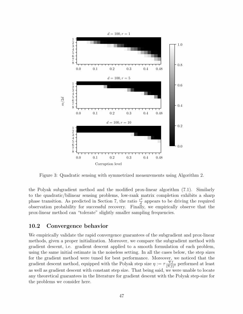
0.0 0.1 0.2 0.3 0.4 0.48

12345678

d = 100, r = 1

0.0 0.1 0.2 0.3 0.4 0.48

12345678

d = 100, r = 5

0.0 0.1 0.2 0.3 0.4 0.48

12345678

d = 100, r = 10

0.0

0.2

0.4

0.6

0.8

1.0

Corruption level

m/2d

Figure 3: Quadratic sensing with symmetrized measurements using Algorithm 2.

the Polyak subgradient method and the modified prox-linear algorithm (7.1). Similarlyto the quadratic/bilinear sensing problems, low-rank matrix completion exhibits a sharpphase transition. As predicted in Section 7, the ratio r2

dappears to be driving the required

observation probability for successful recovery. Finally, we empirically observe that theprox-linear method can “tolerate” slightly smaller sampling frequencies.

10.2 Convergence behavior

We empirically validate the rapid convergence guarantees of the subgradient and prox-linearmethods, given a proper initialization. Moreover, we compare the subgradient method withgradient descent, i.e. gradient descent applied to a smooth formulation of each problem,using the same initial estimate in the noiseless setting. In all the cases below, the step sizesfor the gradient method were tuned for best performance. Moreover, we noticed that thegradient descent method, equipped with the Polyak step size η := τ ∇f

‖∇f‖2 performed at least

as well as gradient descent with constant step size. That being said, we were unable to locateany theoretical guarantees in the literature for gradient descent with the Polyak step-size forthe problems we consider here.

47

0.0 0.35 0.75P(δij = 1)

1

2

4

8

16

Ran

kr

d = 80

0.0 0.35 0.75P(δij = 1)

1

2

4

8

16

Ran

kr

d = 80

Figure 4: Robust PCA using the subgradient method, Algorithm 2, (top) and the modifiedprox-linear method (8.5) (bottom).

0.02 0.20 0.40 0.60P(δij = 1)

12481632

Ran

kr

d = 100

0.02 0.20 0.40 0.60P(δij = 1)

12481632

Ran

kr

d = 100

Figure 5: Low-rank matrix completion using the subgradient method, Algorithm 1 (top),and the modified prox-linear method (7.1) (bottom).

Quadratic and Bilinear sensing. For the quadratic and bilinear sensing problems, weapply gradient descent on the smooth formulations

1

m

∥∥A(XX>)− b∥∥2

2and

1

m‖A(XY )− b‖2

2 .

In Figure 6, we plot the performance of Algorithm 2 for matrix sensing problems with dif-ferent rank / corruption level; remarkably, the level of noise does not significantly affect the

48

rate of convergence. Additionally, the convergence behavior is almost identical for the twoproblems for similar rank/noise configurations. Figure 7 depicts the behavior of Algorithm 1versus gradient descent with empirically tuned step sizes. The subgradient method signifi-cantly outperforms gradient descent. For completeness, we also depict the convergence rateof Algorithm 3 for both problems in Figure 8, where we solve the proximal subproblemsapproximately.

0 200 400 600

10−8

10−6

10−4

10−2

100

k

‖XkX> k−

M]‖ F

/‖M

]‖ F

(r, pfail) = (5, 0.25)

(r, pfail) = (10, 0.25)

(r, pfail) = (5, 0.40)

(r, pfail) = (10, 0.40)

0 200 400 600

10−8

10−6

10−4

10−2

100

k

‖UkV> k−

M]‖ F

/‖M

]‖ F

(r, pfail) = (5, 0.25)

(r, pfail) = (10, 0.25)

(r, pfail) = (5, 0.40)

(r, pfail) = (10, 0.40)

Figure 6: Quadratic (left) and bilinear (right) matrix sensing with d = 200,m = 8 · rd, usingthe subgradient method, Algorithm 2.

0 50 100 150 200 250 300

10−8

10−6

10−4

10−2

100

k

‖XkX> k−

M]‖ F

/‖M

]‖ F

r = 5 r = 10

0 20 40 60 80 100

10−8

10−6

10−4

10−2

100

k

‖UkV> k−

M]‖ F

/‖M

]‖ F

r = 5 r = 10

Figure 7: Algorithm 1 (solid lines) against gradient descent (dashed lines) with step size η.Left: quadratic sensing, η = 10−4. Right: bilinear sensing, η = 10−3.

Matrix completion. In our comparison with smooth methods, we apply gradient descenton the following minimization problem:

minX∈Rd×r:‖X‖2,∞≤C

∥∥ΠΩ(XX>)− ΠΩ(M)∥∥2

F. (10.1)

49

0 2 4 6 8 10 12 14 16

10−9

10−7

10−5

10−3

10−1

k

‖XkX> k−M

]‖ F

/‖M

]‖ F

(r, pfail) = (5, 0.25)

(r, pfail) = (5, 0.40)

(r, pfail) = (10, 0.25)

(r, pfail) = (10, 0.40)

0 2 4 6 8 10 12 14 1610−9

10−7

10−5

10−3

10−1

k

‖UkV> k−M

]‖ F

/‖M

]‖ F

(r, pfail) = (5, 0.25)

(r, pfail) = (5, 0.40)

(r, pfail) = (10, 0.25)

(r, pfail) = (10, 0.40)

Figure 8: Quadratic (left) and bilinear (right) matrix sensing with d = 100,m = 8 · rd, usingthe prox-linear method, Algorithm 3.

Figure 9 depicts the convergence behavior of Algorithm 1 (solid lines) versus gradient descentapplied to Problem (10.1) with a tuned step size η = 0.004 (dashed lines), initialized underthe same conditions for low-rank matrix completion instances. As the theory suggests, highersampling frequency implies better convergence rates. The subgradient method outperformsgradient descent in all regimes.

0 50 100 150 200 250

10−8

10−6

10−4

10−2

100

k

‖XkX> k−

M]‖ F

/‖M

]‖ F

p = 0.1 p = 0.15 p = 0.2

0 50 100 150 200 250

10−8

10−6

10−4

10−2

100

k

‖XkX> k−

M]‖ F

/‖M

]‖ F

p = 0.1 p = 0.15 p = 0.2

Figure 9: Low rank matrix completion with d = 100. Left: r = 4, right: r = 8. Solid linesuse Algorithm 1, dashed lines use gradient descent with step η = 0.004.

Figure 10 depicts the performance of the modified prox-linear method (7.1) in the samesetting as Figure 9. In most cases, the prox-linear algorithm converges within just 15 itera-tions, at what appears to be a rapid linear rate of convergence. Each convex subproblem issolved using a variant of the graph-splitting ADMM algorithm [48].

Robust PCA. For the robust PCA problem, we consider different rank/corruption levelconfigurations to better understand how they affect convergence for the subgradient and

50

0 5 10 15 20

10−8

10−6

10−4

10−2

100

k

‖XkX> k−

M]‖ F

/‖M

]‖ F

p = 0.05p = 0.1p = 0.15p = 0.2

0 5 10 15 20 25

10−8

10−6

10−4

10−2

100

k

‖XkX> k−

M]‖ F

/‖M

]‖ F

p = 0.05p = 0.1p = 0.15p = 0.2

Figure 10: Low rank matrix completion with d = 100 using the modified prox-linear Algo-rithm (7.1). Left: r = 4, right: r = 8.

prox-linear methods, using the non-Euclidean formulation of Section 8.2. We depict allconfigurations in the same plot for a fixed optimization algorithm to better demonstratethe effect of each parameter, as shown in Figure 11. The parameters of the prox-linearmethod are chosen in the same way reported in Section 10.1. In particular, our numericalexperiments appear to support our sharpness Conjecture 8.6 for the robust PCA problem.

0 200 400 600 800 1,000

10−8

10−6

10−4

10−2

100

k

‖XkX> k−

M]‖ 1/‖M

]‖ 1

r = 4 p = 0.0r = 8 p = 0.1r = 16 p = 0.2

0 5 10 15 2010−9

10−7

10−5

10−3

10−1

k

‖XkX> k−

M]‖ 1/‖M

]‖ 1

r = 4 p = 0.0r = 8 p = 0.1r = 16 p = 0.2

Figure 11: `1-robust PCA with d = 100 and p := P(δij = 1). Left: Algorithm 2, right:Algorithm (7.1).

10.2.1 Recovery up to tolerance

In this last section, we test the performance of the prox-linear method and the modifiedPolyak subgradient method (Algorithm 4) for the quadratic sensing and matrix completionproblems, under a dense noise model of Section 9. In the former setting, we set pfail = 0.25, so1/4th of our measurements is corrupted with large magnitude noise. For matrix completion,we observe p = 25% of the entries. In both settings, we add Gaussian noise e which is rescaled

51

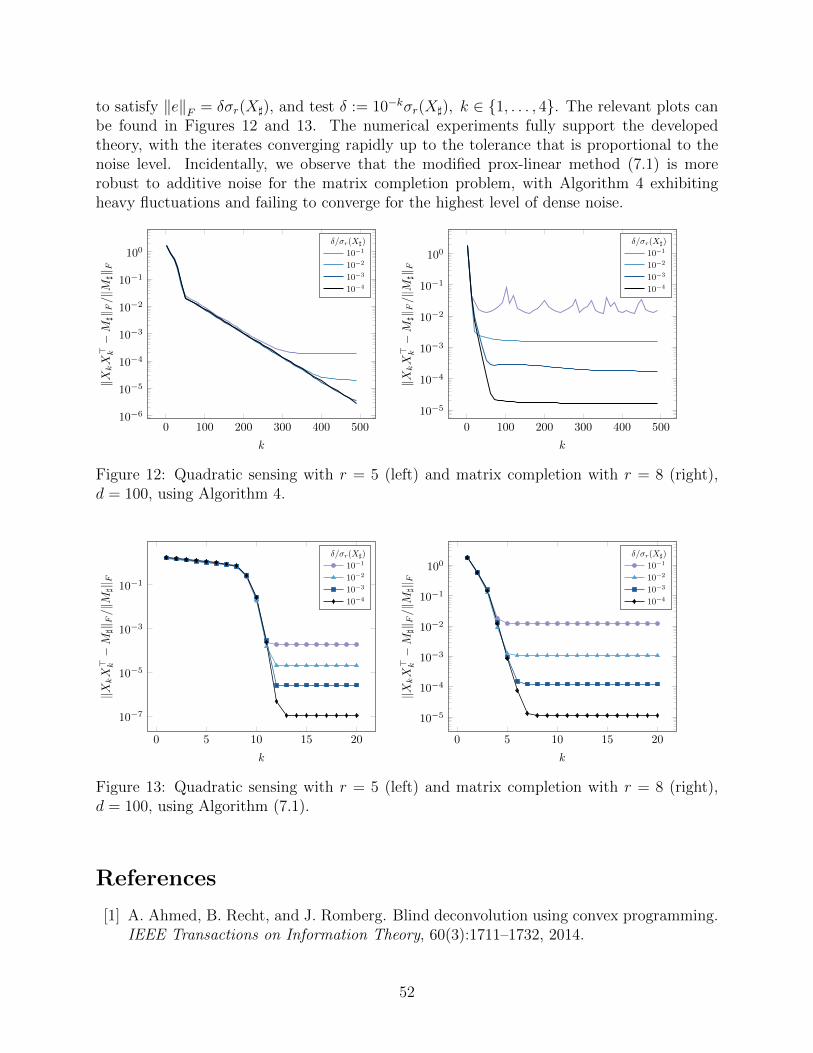
to satisfy ‖e‖F = δσr(X]), and test δ := 10−kσr(X]), k ∈ 1, . . . , 4. The relevant plots canbe found in Figures 12 and 13. The numerical experiments fully support the developedtheory, with the iterates converging rapidly up to the tolerance that is proportional to thenoise level. Incidentally, we observe that the modified prox-linear method (7.1) is morerobust to additive noise for the matrix completion problem, with Algorithm 4 exhibitingheavy fluctuations and failing to converge for the highest level of dense noise.

0 100 200 300 400 50010−6

10−5

10−4

10−3

10−2

10−1

100

k

‖XkX> k−M

]‖ F/‖M

]‖ F

δ/σr(X])

10−1

10−2

10−3

10−4

0 100 200 300 400 500

10−5

10−4

10−3

10−2

10−1

100

k

‖XkX> k−M

]‖ F/‖M

]‖ F

δ/σr(X])

10−1

10−2

10−3

10−4

Figure 12: Quadratic sensing with r = 5 (left) and matrix completion with r = 8 (right),d = 100, using Algorithm 4.

0 5 10 15 20

10−7

10−5

10−3

10−1

k

‖XkX> k−M

]‖ F/‖M

]‖ F

δ/σr(X])

10−1

10−2

10−3

10−4

0 5 10 15 20

10−5

10−4

10−3

10−2

10−1

100

k

‖XkX> k−M

]‖ F/‖M

]‖ F

δ/σr(X])

10−1

10−2

10−3

10−4

Figure 13: Quadratic sensing with r = 5 (left) and matrix completion with r = 8 (right),d = 100, using Algorithm (7.1).

References

[1] A. Ahmed, B. Recht, and J. Romberg. Blind deconvolution using convex programming.IEEE Transactions on Information Theory, 60(3):1711–1732, 2014.

52

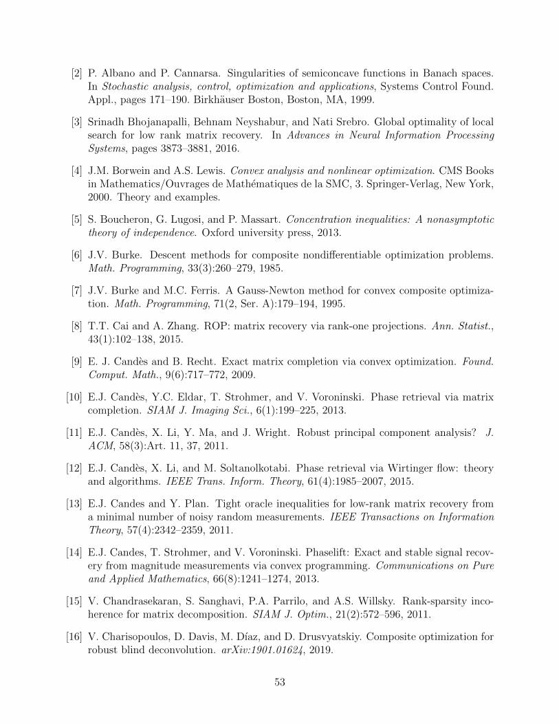
[2] P. Albano and P. Cannarsa. Singularities of semiconcave functions in Banach spaces.In Stochastic analysis, control, optimization and applications, Systems Control Found.Appl., pages 171–190. Birkhauser Boston, Boston, MA, 1999.

[3] Srinadh Bhojanapalli, Behnam Neyshabur, and Nati Srebro. Global optimality of localsearch for low rank matrix recovery. In Advances in Neural Information ProcessingSystems, pages 3873–3881, 2016.

[4] J.M. Borwein and A.S. Lewis. Convex analysis and nonlinear optimization. CMS Booksin Mathematics/Ouvrages de Mathematiques de la SMC, 3. Springer-Verlag, New York,2000. Theory and examples.

[5] S. Boucheron, G. Lugosi, and P. Massart. Concentration inequalities: A nonasymptotictheory of independence. Oxford university press, 2013.

[6] J.V. Burke. Descent methods for composite nondifferentiable optimization problems.Math. Programming, 33(3):260–279, 1985.

[7] J.V. Burke and M.C. Ferris. A Gauss-Newton method for convex composite optimiza-tion. Math. Programming, 71(2, Ser. A):179–194, 1995.

[8] T.T. Cai and A. Zhang. ROP: matrix recovery via rank-one projections. Ann. Statist.,43(1):102–138, 2015.

[9] E. J. Candes and B. Recht. Exact matrix completion via convex optimization. Found.Comput. Math., 9(6):717–772, 2009.

[10] E.J. Candes, Y.C. Eldar, T. Strohmer, and V. Voroninski. Phase retrieval via matrixcompletion. SIAM J. Imaging Sci., 6(1):199–225, 2013.

[11] E.J. Candes, X. Li, Y. Ma, and J. Wright. Robust principal component analysis? J.ACM, 58(3):Art. 11, 37, 2011.

[12] E.J. Candes, X. Li, and M. Soltanolkotabi. Phase retrieval via Wirtinger flow: theoryand algorithms. IEEE Trans. Inform. Theory, 61(4):1985–2007, 2015.

[13] E.J. Candes and Y. Plan. Tight oracle inequalities for low-rank matrix recovery froma minimal number of noisy random measurements. IEEE Transactions on InformationTheory, 57(4):2342–2359, 2011.

[14] E.J. Candes, T. Strohmer, and V. Voroninski. Phaselift: Exact and stable signal recov-ery from magnitude measurements via convex programming. Communications on Pureand Applied Mathematics, 66(8):1241–1274, 2013.

[15] V. Chandrasekaran, S. Sanghavi, P.A. Parrilo, and A.S. Willsky. Rank-sparsity inco-herence for matrix decomposition. SIAM J. Optim., 21(2):572–596, 2011.

[16] V. Charisopoulos, D. Davis, M. Dıaz, and D. Drusvyatskiy. Composite optimization forrobust blind deconvolution. arXiv:1901.01624, 2019.

53

[17] Y. Chen and E.J. Candes. Solving random quadratic systems of equations is nearly aseasy as solving linear systems. Comm. Pure Appl. Math., 70(5):822–883, 2017.

[18] Y. Chen, Y. Chi, and A.J. Goldsmith. Exact and stable covariance estimation fromquadratic sampling via convex programming. IEEE Trans. Inform. Theory, 61(7):4034–4059, 2015.

[19] Y. Chen and M.J. Wainwright. Fast low-rank estimation by projected gradient descent:General statistical and algorithmic guarantees. arXiv:1509.03025, 2015.

[20] Y. Chi, Y.M. Lu, and Y. Chen. Nonconvex optimization meets low-rank matrix factor-ization: An overview. arXiv:1809.09573, 2018.

[21] M.A. Davenport and J. Romberg. An overview of low-rank matrix recovery from incom-plete observations. IEEE Journal of Selected Topics in Signal Processing, 10(4):608–622,June 2016.

[22] D. Davis and D. Drusvyatskiy. Stochastic model-based minimization of weakly convexfunctions. SIAM Journal on Optimization, 29(1):207–239, 2019.

[23] D. Davis, D. Drusvyatskiy, K.J. MacPhee, and C. Paquette. Subgradient methods forsharp weakly convex functions. J. Optim. Theory Appl., 179(3):962–982, 2018.

[24] D. Davis, D. Drusvyatskiy, and C. Paquette. The nonsmooth landscape of phase re-trieval. To appear in IMA J. Numer. Anal., arXiv:1711.03247, 2017.

[25] D. Drusvyatskiy and A.S. Lewis. Error bounds, quadratic growth, and linear conver-gence of proximal methods. Math. Oper. Res., 43(3):919–948, 2018.

[26] D. Drusvyatskiy and C. Paquette. Efficiency of minimizing compositions of convexfunctions and smooth maps. Math. Prog., pages 1–56, 2018.

[27] J.C. Duchi and F. Ruan. Solving (most) of a set of quadratic equalities: com-posite optimization for robust phase retrieval. IMA J. Information and Inference,doi:10.1093/imaiai/iay015, 2018.

[28] J.C. Duchi and F. Ruan. Stochastic methods for composite and weakly convex opti-mization problems. SIAM J. Optim., 28(4):3229–3259, 2018.

[29] Y.C. Eldar and S. Mendelson. Phase retrieval: stability and recovery guarantees. Appl.Comput. Harmon. Anal., 36(3):473–494, 2014.

[30] M. Fazel. Matrix Rank Minimization with Applications. PhD thesis, Stanford University,2002.

[31] R. Fletcher. A model algorithm for composite nondifferentiable optimization problems.Math. Programming Stud., (17):67–76, 1982. Nondifferential and variational techniquesin optimization (Lexington, Ky., 1980).

54

[32] R. Ge, C. Jin, and Y. Zheng. No spurious local minima in nonconvex low rank problems:A unified geometric analysis. In Proceedings of the 34th International Conference onMachine Learning-Volume 70, pages 1233–1242. JMLR. org, 2017.

[33] Rong Ge, Jason D Lee, and Tengyu Ma. Matrix completion has no spurious localminimum. In D. D. Lee, M. Sugiyama, U. V. Luxburg, I. Guyon, and R. Garnett, edi-tors, Advances in Neural Information Processing Systems 29, pages 2973–2981. CurranAssociates, Inc., 2016.

[34] J.L. Goffin. On convergence rates of subgradient optimization methods. Math. Pro-gramming, 13(3):329–347, 1977.

[35] T. Goldstein and C. Studer. Phasemax: Convex phase retrieval via basis pursuit. IEEETransactions on Information Theory, 64(4):2675–2689, April 2018.

[36] T. Klein and E. Rio. Concentration around the mean for maxima of empirical processes.The Annals of Probability, 33(3):1060–1077, 2005.

[37] A.S. Lewis and S.J. Wright. A proximal method for composite minimization. Math.Program., 158(1-2, Ser. A):501–546, 2016.

[38] X. Li, S. Ling, T. Strohmer, and K. Wei. Rapid, robust, and reliable blind deconvolutionvia nonconvex optimization. arXiv:1606.04933, 2016.

[39] X. Li, Z. Zhu, A.M.-C. So, and R. Vidal. Nonconvex robust low-rank matrix recovery.arXiv:1809.09237, 2018.

[40] Y. Li, C. Ma, Y. Chen, and Y. Chi. Nonconvex matrix factorization from rank-onemeasurements. arXiv:1802.06286, 2018.

[41] S. Ling and T. Strohmer. Self-calibration and biconvex compressive sensing. InverseProblems, 31(11):115002, 31, 2015.

[42] C. Ma, K. Wang, Y. Chi, and Y. Chen. Implicit regularization in nonconvex statisticalestimation: Gradient descent converges linearly for phase retrieval and matrix comple-tion. In Jennifer Dy and Andreas Krause, editors, Proceedings of the 35th InternationalConference on Machine Learning, volume 80 of Proceedings of Machine Learning Re-search, pages 3345–3354, Stockholmsmssan, Stockholm Sweden, 10–15 Jul 2018. PMLR.

[43] S. Mendelson. A remark on the diameter of random sections of convex bodies. InGeometric aspects of functional analysis, volume 2116 of Lecture Notes in Math., pages395–404. Springer, Cham, 2014.

[44] S. Mendelson. Learning without concentration. J. ACM, 62(3):Art. 21, 25, 2015.

[45] B. S. Mordukhovich. Variational Analysis and Generalized Differentiation I: BasicTheory. Grundlehren der mathematischen Wissenschaften, Vol 330, Springer, Berlin,2006.

55

[46] S.N. Negahban, P. Ravikumar, M.J. Wainwright, and B. Yu. A unified framework forhigh-dimensional analysis of M -estimators with decomposable regularizers. Statist. Sci.,27(4):538–557, 2012.

[47] E.A. Nurminskii. The quasigradient method for the solving of the nonlinear program-ming problems. Cybernetics, 9(1):145–150, Jan 1973.

[48] N. Parikh and S. Boyd. Block splitting for distributed optimization. MathematicalProgramming Computation, 6(1):77–102, 2014.

[49] R.A. Poliquin and R.T. Rockafellar. Prox-regular functions in variational analysis.Trans. Amer. Math. Soc., 348:1805–1838, 1996.

[50] B. Recht, M. Fazel, and P.A. Parrilo. Guaranteed minimum-rank solutions of linearmatrix equations via nuclear norm minimization. SIAM Rev., 52(3):471–501, 2010.

[51] R.T. Rockafellar. Favorable classes of Lipschitz-continuous functions in subgradientoptimization. In Progress in nondifferentiable optimization, volume 8 of IIASA Collab-orative Proc. Ser. CP-82, pages 125–143. Int. Inst. Appl. Sys. Anal., Laxenburg, 1982.

[52] R.T. Rockafellar and R.J-B. Wets. Variational Analysis. Grundlehren der mathematis-chen Wissenschaften, Vol 317, Springer, Berlin, 1998.

[53] S. Rolewicz. On paraconvex multifunctions. In Third Symposium on Operations Re-search (Univ. Mannheim, Mannheim, 1978), Section I, volume 31 of Operations Res.Verfahren, pages 539–546. Hain, Konigstein/Ts., 1979.

[54] M. Rudelson and R. Vershynin. Small ball probabilities for linear images of high-dimensional distributions. International Mathematics Research Notices, 2015(19):9594–9617, 2014.

[55] Y. Shechtman, Y.C. Eldar, O. Cohen, H.N. Chapman, J. Miao, and M. Segev. Phaseretrieval with application to optical imaging: A contemporary overview. IEEE SignalProcessing Magazine, 32(3):87–109, May 2015.

[56] R. Sun and Z.-Q. Luo. Guaranteed matrix completion via non-convex factorization.IEEE Trans. Inform. Theory, 62(11):6535–6579, 2016.

[57] S. Tu, R. Boczar, M. Simchowitz, M. Soltanolkotabi, and B. Recht. Low-rank solutionsof linear matrix equations via Procrustes flow. In Proceedings of the 33rd InternationalConference on International Conference on Machine Learning - Volume 48, ICML’16,pages 964–973. JMLR.org, 2016.

[58] Roman Vershynin. High-Dimensional Probability: An Introduction with Applications inData Science. Cambridge University Press, 2018.

[59] X. Yi, D. Park, Y. Chen, and C. Caramanis. Fast algorithms for robust pca via gradientdescent. In Advances in neural information processing systems, pages 4152–4160, 2016.

56

A Proofs in Section 5

In this section, we prove rapid local convergence guarantees for the subgradient and prox-linear algorithms under regularity conditions that hold only locally around a particularsolution. We will use the Euclidean norm throughout this section; therefore to simplify thenotation, we will drop the subscript two. Thus ‖ · ‖ denotes the `2 on a Euclidean space Ethroughout.

We will need the following quantitative version of Lemma 5.1.

Lemma A.1. Suppose Assumption E holds and let γ ∈ (0, 2) be arbitrary. Then for anypoint x ∈ Bε/2(x) ∩ Tγ\X ∗, the estimate holds:

dist (0, ∂f(x)) ≥(1− γ

2

)µ.

Proof. Consider any point x ∈ Bε/2(x) satisfying dist(x,X ∗) ≤ γ µρ. Let x∗ ∈ projX ∗(x) be

arbitrary and note x∗ ∈ Bε(x). Thus for any ζ ∈ ∂f(x) we deduce

µ · dist(x,X ∗) ≤ f(x)− f(x∗) ≤ 〈ζ, x− x∗〉+ρ

2‖x− x∗‖2 ≤ ‖ζ‖dist(x,X ∗) +

ρ

2dist2(x,X ∗).

Therefore we deduce the lower bound on the subgradients ‖ζ‖ ≥ µ − ρ2· dist(x,X ∗) ≥(

1− γ2

)µ, as claimed.

A.1 Proof of Theorem 5.6

Let k be the first index (possibly infinite) such that xk /∈ Bε/2(x). We claim that (5.4) holdsfor all i < k. We show this by induction. To this end, suppose (5.4) holds for all indices upto i− 1. In particular, we deduce dist(xi,X ∗) ≤ dist(x0,X ∗) ≤ µ

2ρ. Let x∗ ∈ projX ∗(xi) and

note x∗ ∈ Bε(x), since

‖x∗ − x‖ ≤ ‖x∗ − xi‖+ ‖xi − x‖ ≤ 2‖xi − x‖ ≤ ε.

57

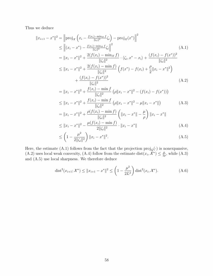
Thus we deduce

‖xi+1 − x∗‖2 =∥∥∥projX

(xi − f(xi)−minX f

‖ζi‖2 ζi

)− projX (x∗)

∥∥∥2

≤∥∥∥(xi − x∗)− f(xi)−minX f

‖ζi‖2 ζi

∥∥∥2

(A.1)

= ‖xi − x∗‖2 +2(f(xi)−minX f)

‖ζi‖2· 〈ζi, x∗ − xi〉+

(f(xi)− f(x∗))2

‖ζi‖2

≤ ‖xi − x∗‖2 +2(f(xi)−min f)

‖ζi‖2

(f(x∗)− f(xi) +

ρ

2‖xi − x∗‖2

)+

(f(xi)− f(x∗))2

‖ζi‖2(A.2)

= ‖xi − x∗‖2 +f(xi)−min f

‖ζi‖2

(ρ‖xi − x∗‖2 − (f(xi)− f(x∗))

)≤ ‖xi − x∗‖2 +

f(xi)−min f

‖ζi‖2

(ρ‖xi − x∗‖2 − µ‖xi − x∗‖

)(A.3)

= ‖xi − x∗‖2 +ρ(f(xi)−min f)

‖ζi‖2

(‖xi − x∗‖ −

µ

ρ

)‖xi − x∗‖

≤ ‖xi − x∗‖2 − µ(f(xi)−min f)

2‖ζi‖2· ‖xi − x∗‖ (A.4)

≤(

1− µ2

2‖ζi‖2

)‖xi − x∗‖2. (A.5)

Here, the estimate (A.1) follows from the fact that the projection projQ(·) is nonexpansive,(A.2) uses local weak convexity, (A.4) follow from the estimate dist(xi,X ∗) ≤ µ

2ρ, while (A.3)

and (A.5) use local sharpness. We therefore deduce

dist2(xi+1;X ∗) ≤ ‖xi+1 − x∗‖2 ≤(

1− µ2

2L2

)dist2(xi,X ∗). (A.6)

58

Thus (5.4) holds for all indices up to k − 1. We next show that k is infinite. To this end,observe

‖xk − x0‖ ≤k−1∑i=0

‖xi+1 − xi‖ =k−1∑i=0

∥∥∥projX

(xi − f(xi)−minX f

‖ζi‖2 ζi

)− projX (xi)

∥∥∥≤

k−1∑i=0

f(xi)−minX f

‖ζi‖

≤k−1∑i=0

⟨ζi‖ζi‖ , xi − projX ∗(xi)

⟩+

ρ

2‖ζi‖‖xi − projX ∗(xi)‖2

≤k−1∑i=0

dist(xi,X ∗) +2ρ

3µdist2(xi,X ∗) (A.7)

≤ 4

3·k−1∑i=0

dist(xi,X ∗) (A.8)

≤ 4

3· dist(x0,X ∗) ·

k−1∑i=0

(1− µ2

2L2

) i2

(A.9)

≤ 16L2

3µ2· dist(x0,X ∗) ≤

ε

4,

where (A.7) follows by Lemma A.1 with γ = 1/2, the bound in (A.8) follows by (A.6) and theassumption on dist(x0,X ∗), finally (A.9) holds thanks to (A.6). Thus applying the triangleinequality we get the contradiction ‖xk − x‖ ≤ ε/2. Consequently all the iterates xk fork = 0, 1, . . . ,∞ lie in Bε/2(x) and satisfy (5.4).

Finally, let x∞ be any limit point of the sequence xi. We then successively compute

‖xk − x∞‖ ≤∞∑i=k

‖xi+1 − xi‖ ≤∞∑i=k

f(xi)−min f

‖ζi‖

≤ 4L

3µ·∞∑i=k

dist(xi,X ∗)

≤ 4L

3µ· dist(x0,X ∗) ·

∞∑i=k

(1− µ2

2L2

) i2

≤ 16L3

3µ3· dist(x0,X ∗) ·

(1− µ2

2L2

) k2

.

This completes the proof.

A.2 Proof of Theorem 5.7

Fix an arbitrary index k and observe

‖xk+1 − xk‖ =

∥∥∥∥projQ(xk)− projQ

(xk − αk

ξk‖ξk‖

)∥∥∥∥ ≤ αk = λ · qk.

59

Hence, we conclude the uniform bound on the iterates:

‖xk − x0‖ ≤∞∑i=0

‖xi+1 − xi‖ ≤ λ1−q

and the R-linear rate of convergence

‖xk − x∞‖ ≤∞∑i=k

‖xi+1 − xi‖ ≤ λ1−qq

k,

where x∞ is any limit point of the iterate sequence.Let us now show that the iterates do not escape Bε/2(x). To this end, observe

‖xk − x‖ ≤ ‖xk − x0‖+ ‖x0 − x‖ ≤ λ1−q + ε

4.

We must therefore verify the estimate λ1−q ≤ ε

4, or equivalently γ ≤ ερL(1−γ)τ2

4µ2(1+√

1−(1−γ)τ2). Clearly,

it suffices to verify γ ≤ ερ(1−γ)4L

, which holds by the definition of γ. Thus all the iterates

xk lie in Bε/2(x). Moreover τ ≤√

12≤√

12−γ , the rest of the proof is identical to that

in [23, Theorem 5.1].

A.3 Proof of Theorem 5.8

Fix any index i such that xi ∈ Bε(x) and let x ∈ X be arbitrary. Since the functionz 7→ fxi(z) + β

2‖z − xi‖2 is β-strongly convex and xi+1 is its minimizer, we deduce(

fxi(xi+1) +β

2‖xi+1 − xi‖2

)+β

2‖xi+1 − x‖2 ≤ fxi(x) +

β

2‖x− xi‖2. (A.10)

Setting x = xi and appealing to approximation accuracy, we obtain the descent guarantee

‖xi+1 − xi‖2 ≤ 2

β(f(xi)− f(xi+1)). (A.11)

In particular, the function values are decreasing along the iterate sequence. Next choosingany x∗ ∈ projX ∗(xi) and setting x = x∗ in (A.10) yields(

fxi(xi+1) +β

2‖xi+1 − xi‖2

)+β

2‖xi+1 − x∗‖2 ≤ fxi(x

∗) +β

2‖x∗ − xi‖2.

Appealing to approximation accuracy and lower-bounding β2‖xi+1−x∗‖2 by zero, we conclude

f(xi+1) ≤ f(x∗) + β‖x∗ − xi‖2. (A.12)

Using sharpness we deduce the contraction guarantee

f(xi+1)− f(x∗) ≤ β · dist2(xi,X ∗)

≤ β

µ2(f(xi)− f(x∗))2

≤ β(f(xi)− f(x∗))

µ2· (f(xi)− f(x∗)) ≤ 1

2· (f(xi)− f(x∗)),

(A.13)

60

where the last inequality uses the assumption f(x0) −minX f ≤ µ2

2β. Let k > 0 be the first

index satisfying xk /∈ Bε(x). We then deduce

‖xk − x0‖ ≤k−1∑i=0

‖xi+1 − xi‖ ≤√

2

β·k−1∑i=0

√f(xi)− f(xi+1) (A.14)

≤√

2

β·k−1∑i=0

√f(xi)− f(x∗)

≤√

2

β·√f(x0)− f(x∗) ·

k−1∑i=0

(1

2

) i2

(A.15)

≤ 1√2− 1

√f(x0)− f(x∗)

β≤ ε/2,

where (A.14) follows from (A.11) and (A.15) follows from (A.13). Thus we conclude ‖xk −x‖ ≤ ε, which is a contradiction. Therefore all the iterates xk, for k = 0, 1, . . . ,∞, liein Bε(x). Combing this with (A.12) and sharpness yields the claimed quadratic convergeguarantee

µ · dist(xk+1,X ∗) ≤ f(xk+1)− f(x) ≤ β · dist2(xk,X ).

Finally, let x∞ be any limit point of the sequence xi. We then deduce

‖xk − x∞‖ ≤∞∑i=k

‖xi+1 − xi‖ ≤√

2

β·∞∑i=k

√f(xi)− f(xi+1)

≤√

2

β·∞∑i=k

√f(xi)−min

Xf

≤ µ√

2

β·∞∑i=k

(β

µ2(f(x0)−min f)

)2i−1

(A.16)

≤ µ√

2

β·∞∑i=k

(1

2

)2i−1

≤ µ√

2

β

∞∑j=0

(1

2

)2k−1+j

≤ 2√

2µ

β·(

1

2

)2k−1

,

where (A.16) follows from (A.13). The theorem is proved.

B Proofs in Section 6

B.1 Proof of Lemma 6.3

In order to prove that the assumption in each case, we will prove a stronger “small-ballcondition” [43,44], which immediately implies the claimed lower bounds on the expectationby Markov’s inequality. More precisely, we will show that there exist numerical constantsµ0, p0 > 0 such that

61

1. (Matrix Sensing)inf

M : Rank M≤2r‖M‖F=1

P(|〈P,M〉| ≥ µ0) ≥ p0,

2. (Quadratic Sensing I)

infM∈Sd: Rank M≤2r

‖M‖F=1

P(|p>Mp| ≥ µ0) ≥ p0,

3. (Quadratic Sensing II)

infM∈Sd: Rank M≤2r

‖M‖F=1

P(|p>Mp− p>Mp| ≥ µ0

)≥ p0,

4. (Bilinear Sensing)inf

M : Rank M≤2r‖M‖F=1

P(|p>Mq| ≥ µ0) ≥ p0.

These conditions immediately imply Assumptions G-J. Indeed, by Markov’s inequality,in the case of matrix sensing we deduce

E|〈P,M〉| ≥ µ0P (|〈P,M〉| > µ0) ≥ µ0p0.

The same reasoning applies to all the other problems.

Matrix sensing. Consider any matrix M with ‖M‖F = 1. Then, since g := 〈P,M〉 followsa standard normal distribution, we may set µ0 to be the median of |g| and p0 = 1/2 to obtain

infM : Rank M≤2r‖M‖F=1

P(|〈P,M〉| ≥ µ0) = P(|g| ≥ µ0) ≥ p0.

Quadratic Sensing I. Fix a matrix M with Rank M ≤ 2r and ‖M‖F = 1. Let M =UDU> be an eigenvalue decomposition of M . Using the rotational invariance of the Gaussiandistribution, we deduce

p>Mpd= p>Dp =

2r∑k=1

λkp2k,

whered= denotes equality in distribution. Next, let z be a standard normal variable. We

will now invoke Proposition F.2. Let C > 0 be the numerical constant appearing in theproposition. Notice that the function φ : R+ → R given by

φ(t) = supu∈R

P(|z2 − u| ≤ t)

is continuous and strictly increasing, and it satisfies φ(0) = 0 and limt→∞ φ(t) = 1. Hencewe may set µ0 = φ−1(min1/2C, 1/2). Proposition F.2 then yields

P(|p>Mp| ≤ µ0) = P

(∣∣∣∣∣2r∑k=1

λkp2k

∣∣∣∣∣ ≤ µ0

)≤ sup

u∈RP

(∣∣∣∣∣2r∑k=1

λkp2k − u

∣∣∣∣∣ ≤ µ0

)≤ Cφ(µ0) ≤ 1

2.

By taking the supremum of both sides of the inequality we conclude that Assumption Hholds with µ0 and p0 = 1/2.

62

Quadratic sensing II. Let M = UDU> be an eigenvalue decomposition of M . Using therotational invariance of the Gaussian distribution, we deduce

p>Mp− p>Mpd= p>Dp− p>Dp =

2r∑k=1

λk(p2k − p2

k

) d= 2

2r∑k=1

λkpkpk,

where the last relation follows since (pk − pk) , (pk + pk) are independent standard normalrandom variables with mean zero and variance two. We will now invoke Proposition F.2. LetC > 0 be the numerical constant appearing in the proposition. Let z and z be independentstandard normal variables. Notice that the function φ : R+ → R given by

φ(t) = supu∈R

P(|2zz − u| ≤ t)

is continuous, strictly increasing, satisfies φ(0) = 0 and approaches one at infinity. Definingµ0 = φ−1(min1/2C, 1/2) and applying Proposition F.2, we get

P

(∣∣∣∣∣22r∑k=1

σkpkpk

∣∣∣∣∣ ≤ µ0

)≤ sup

u∈RP

(∣∣∣∣∣22r∑k=1

σkpkpk − u∣∣∣∣∣ ≤ µ0

)≤ Cφ(µ0) ≤ 1

2.

By taking the supremum of both sides of the inequality we conclude that Assumption I holdswith µ0 and p0 = 1/2.

We omit the details for the bilinear case, which follow by similar arguments.

B.2 Proof of Theorem 6.4

The proofs in this section rely on the following proposition, which shows that that pointwiseconcentration imply uniform concentration. We defer the proof to Appendix B.3.

Proposition B.1. Let A : Rd1×d2 → Rm be a random linear mapping with property that forany fixed matrix M ∈ Rd1×d2 of rank at most 2r with norm ‖M‖F = 1 and any fixed subsetof indices I ⊆ 1, . . . ,m satisfying |I| < m/2, the following hold:

(1) The measurements A(M)1, . . . ,A(M)m are i.i.d.

(2) RIP holds in expected value:

α ≤ E|A(M)i| ≤ β(r) for all i ∈ 1, . . . ,m (B.1)

where α > 0 is a universal constant and β is a positive-valued function that couldpotentially depend on the rank of M .

(3) There exist a universal constant K > 0 and a positive-valued function c(m, r) such thatfor any t ∈ [0, K] the deviation bound

1

m

∣∣‖AIc(M)‖1 − ‖AI(M)‖1 − E[‖AIc(M)‖1 − ‖AI(M)‖1

]∣∣ ≤ t (B.2)

holds with probability at least 1− 2 exp(−t2c(m, r)).

63

Then, there exist universal constants c1, . . . , c6 > 0 depending only on α and K such that ifI ⊆ 1, . . . ,m is a fixed subset of indices satisfying |I| < m/2 and

c(m, r) ≥ c1

(1− 2|I|/m)2r(d1 + d2 + 1) ln

(c2 +

c2β(r)

1− 2|I|/m

)then with probability at least 1−4 exp (−c3(1− 2|I|/m)2c(m, r)) every matrix M ∈ Rd1×d2ofrank at most 2r satisfies

c4‖M‖F ≤1

m‖A(M)‖1 ≤ c5β(r)‖M‖F , (B.3)

and

c6

(1− 2|I|

m

)‖M‖F ≤

1

m(‖AIc(M)‖1 − ‖AIM‖1) . (B.4)

Due to scale invariance of the above result, we need only verify its assumptions in thecase that ‖M‖F = 1. We implicitly use this observation below.

B.2.1 Part 1 of Theorem 6.4 (Matrix sensing)

Lemma B.2. The random variable |〈P,M〉| is sub-gaussian with parameter Cη. Conse-quently,

α ≤ E|〈P,M〉| . η. (B.5)

Moreover, there exists a universal constant c > 0 such that for any t ∈ [0,∞) the deviationbound

1

m

∣∣‖AIc(M)‖1 − ‖AI(M)‖1 − E[‖AIc(M)‖1 − ‖AI(M)‖1

]∣∣ ≤ t (B.6)

holds with probability at least 1− 2 exp(− ct2

η2m).

Proof. Assumption G immediately implies the lower bound in (B.5). To prove the upperbound, first note that by assumption we have

‖〈P,M〉‖ψ2 . η.

This bound has two consequences, first 〈P,M〉 is a sub-gaussian random variable with pa-rameter η and second E|〈P,M〉| . η [58, Proposition 2.5.2]. Thus, we have proved (B.5).

To prove the deviation bound (B.6) we introduce the random variables

Yi =

|〈Pi,M〉| − E|〈Pi,M〉| if i /∈ I, and

− (|〈Pi,M〉| − E|〈Pi,M〉|) otherwise.

Since |〈Pi,M〉| is sub-gaussian, we have ‖Yi‖ψ2 . η for all i, see [58, Lemma 2.6.8]. Hence,Hoeffding’s inequality for sub-gaussian random variables [58, Theorem 2.6.2] gives the desiredupper bound on P

(1m|∑m

i=1 Yi| ≥ t).

Applying Proposition B.1 with β(r) η and c(m, r) m/η2 now yields the result.

64

B.2.2 Part 2 of Theorem 6.4 (Quadratic sensing I)

Lemma B.3. The random variable |p>Mp| is sub-exponential with parameter√

2rη2. Con-sequently,

α ≤ E|p>Mp| .√

2rη2. (B.7)

Moreover, there exists a universal constant c > 0 such that for any t ∈ [0,√

2rη] the deviationbound

1

m

∣∣‖AIc(M)‖1 − ‖AI(M)‖1 − E[‖AIc(M)‖1 − ‖AI(M)‖1

]∣∣ ≤ t (B.8)

holds with probability at least 1− 2 exp(− ct2

η4m/r

).

Proof. Assumption H gives the lower bound in (B.7). To prove the upper bound, first notethat M =

∑2rk=1 σkuku

>k where σk and uk are the kth singular values and vectors of M ,

respectively. Hence

‖p>Mp‖ψ1 =

∥∥∥∥∥p>(

2r∑k=1

σkuku>k

)p

∥∥∥∥∥ψ1

=

∥∥∥∥∥2r∑k=1

σk〈p, uk〉2∥∥∥∥∥ψ1

≤2r∑k=1

σk∥∥〈p, uk〉2∥∥ψ1

≤2r∑k=1

σk ‖〈p, uk〉‖2ψ2

= η2

2r∑k=1

σk ≤√

2rη2,

where the first inequality follows since ‖·‖ψ1 is a norm, the second one follows since ‖XY ‖ψ1 ≤‖X‖ψ2‖Y ‖ψ2 [58, Lemma 2.7.7], and the third inequality holds since ‖σ‖1 ≤

√2r‖σ‖2. This

bound has two consequences, first p>Mp is a sub-exponential random variable with param-eter√rη2 and second Ep>Mp ≤

√2rη2 [58, Exercise 2.7.2]. Thus, we have proved (B.7).

To prove the deviation bound (B.8) we introduce the random variables

Yi =

p>i Mpi − Ep>i Mpi if i /∈ I, and

−(p>i Mpi − Ep>i Mpi

)otherwise.

Since p>Mp is sub-exponential, we have ‖Yi‖ψ1 .√rη2 for all i, see [58, Exercise 2.7.10].

Hence, Bernstein inequality for sub-exponential random variables [58, Theorem 2.8.2] givesthe desired upper bound on P

(1m|∑m

i=1 Yi| ≥ t).

Applying Proposition B.1 with with β(r) √rη2 and c(m, r) m/η4r now yields theresult.

B.2.3 Part 3 of Theorem 6.4 (Quadratic sensing II)

Lemma B.4. The random variable |p>Mp− p>Mp| is sub-exponential with parameter Cη2.Consequently,

α ≤ E|p>Mp− p>Mp| . η2. (B.9)

Moreover, there exists a universal constant c > 0 such that for any t ∈ [0, η2] the deviationbound

1

m

∣∣‖AIc(M)‖1 − ‖AI(M)‖1 − E[‖AIc(M)‖1 − ‖AI(M)‖1

]∣∣ ≤ t (B.10)

holds with probability at least 1− 2 exp(− ct2

η4m).

65

Proof. Assumption I implies the lower bound in (B.9). To prove the upper bound, we willshow that ‖|p>Mp− p>Mp>|‖ψ1 ≤ η2. By definition of the Orlicz norm ‖|X|‖ψ1 = ‖X‖ψ1 forany random variable X, hence without loss of generality we may remove the absolute value.Recall that M =

∑2rk=1 σkuku

>k where σk and uk are the kth singular values and vectors of

M , respectively. Hence, the random variable of interest can be rewritten as

p>Mp− p>Mp>d=

2r∑k=1

σk(〈uk, p〉2 − 〈uk, p〉2

). (B.11)

By assumption the random variables 〈uk, p〉 are η-sub-gaussian, this implies that 〈uk, p〉2 areη2-sub-exponential, since ‖〈uk, p〉2‖ψ1 ≤ ‖〈uk, p〉‖2

ψ2.

Recall the following characterization of the Orlicz norm for mean-zero random variables

‖X‖ψ1 ≤ Q ⇐⇒ E exp(λX) ≤ exp(Q2λ2) for all λ satisfying |λ| ≤ 1/Q2 (B.12)

where the Q Q, see [58, Proposition 2.7.1]. To prove that the random variable (B.11)is sub-exponential we will exploit this characterization. Since each inner product squared〈uk, p〉2 is sub-exponential, the equivalence implies the existence of a constant c > 0 forwhich the uniform bound

E exp(λ〈uk, p〉2) ≤ exp(cη4λ2

)for all k ∈ [2r] and |λ| ≤ 1/cη4 (B.13)

holds. Let λ be an arbitrary scalar with |λ| ≤ 1/cη4, then by expanding the momentgenerating function of (B.11) we get

E exp

(λ

2r∑k=1

σk(〈uk, p〉2 − 〈uk, p〉2

))= E

2r∏k=1

exp(λσk〈uk, p〉2

)exp

(−λσk〈uk, p〉2

)=

2r∏k=1

E exp(λσk〈uk, p〉2

)E exp

(−λσk〈uk, p〉2

)≤

2r∏k=1

exp((cη)2λ2σ2

k

)exp

(cη4λ2σ2

k

)= exp

(2cη4λ2

2r∑k=1

σ2k

)= exp

(2cη4λ2

).

where the inequality follows by (B.13) and the last relation follows since σ is unit norm.Combining this with (B.12) gives

‖|p>Mp− p>Mp>|‖ψ1 . η2.

This bound has two consequences, first |p>Mp− p>Mp>| is a sub-exponential random vari-able with parameter Cη2 and second E|p>Mp − p>Mp>| ≤ Cη2 [58, Exercise 2.7.2]. Thus,we have proved (B.9).

To prove the deviation bound (B.10) we introduce the random variables

Yi =

A(M)i − EA(M)i if i /∈ I, and

− (A(M)i − EA(M)i) otherwise.

66

The sub-exponentiality of A(M)i implies ‖Yi‖ψ1 . η2 for all i, see [58, Exercise 2.7.10].Hence, Bernstein inequality for sub-exponential random variables [58, Theorem 2.8.2] givesthe desired upper bound on P

(1m|∑m

i=1 Yi| ≥ t).

Applying Proposition B.1 with β(r) η2 and c(m, r) m/η4 now yields the result.

B.2.4 Part 4 of Theorem 6.4 (Bilinear sensing)

Lemma B.5. The random variable |p>Mq| is sub-exponential with parameter Cη2. Conse-quently,

α ≤ E|p>Mq| . η2. (B.14)

Moreover, there exists a universal constant c > 0 such that for any t ∈ [0, η2] the deviationbound

1

m

∣∣‖AIc(M)‖1 − ‖AI(M)‖1 − E[‖AIc(M)‖1 − ‖AI(M)‖1

]∣∣ ≤ t (B.15)

holds with probability at least 1− 2 exp(− ct2

η4m).

Proof. As before the lower bound in (B.14) is implied by Assumption J. To prove the upperbound, we will show that ‖|p>Mq|‖ψ1 ≤ η2. By definition of the Orlicz norm ‖|X|‖ψ1 =‖X‖ψ1 for any random variable X, hence we may remove the absolute value. Recall thatM =

∑2rk=1 σkukv

>k where σk and (uk, vk) are the kth singular values and vectors of M ,

respectively. Hence, the random variable of interest can be rewritten as

p>Mqd=

2r∑k=1

σk〈p, uk〉〈vk, q〉. (B.16)

By assumption the random variables 〈p, uk〉 and 〈vk, q〉 are η-sub-gaussian, this implies that〈p, uk〉〈vk, q〉 are η2-sub-exponential.

To prove that the random variable (B.16) is sub-exponential we will again use (B.12).Since each random variable 〈p, uk〉〈vk, q〉 is sub-exponential, the equivalence implies theexistence of a constant c > 0 for which the uniform bound

E exp(λ〈p, uk〉〈vk, q〉) ≤ exp(cη4λ2

)for all k ∈ [2r] and |λ| ≤ 1/cη4 (B.17)

holds. Let λ be an arbitrary scalar with |λ| ≤ 1/cη4, then by expanding the momentgenerating function of (B.16) we get

E exp

(λ

2r∑k=1

σk〈p, uk〉〈vk, q〉)

=2r∏k=1

E exp (λσk〈p, uk〉〈vk, q〉)

≤ exp

(2cη4λ2

r∑k=1

σ2k

)= exp

(2cη4λ2

).

where the inequality follows by (B.17) and the last relation follows since σ is unitary. Com-bining this with (B.12) gives

‖|p>Mq|‖ψ1 . η2.

67

Thus, we have proved (B.14).Once again, to show the deviation bound (B.15) we introduce the random variables

Yi =

|p>i Mqi| − E|p>i Mqi| if i /∈ I, and

−(|p>i Mqi| − E|p>i Mqi|

)otherwise.

and apply Bernstein’s inequality for sub-exponential random variables [58, Theorem 2.8.2]to get the stated upper bound on P

(1m|∑m

i=1 Yi| ≥ t).

Applying Proposition B.1 with β(r) η2 and c(m, r) m/η4 now yields the result.

B.3 Proof of Proposition B.1

Choose ε ∈ (0,√

2) and let N be the (ε/√

2)-net guaranteed by Lemma F.1. Pick somet ∈ (0, K] so that (B.2) can hold, we will fix the value of this parameter later in the proof.Let E denote the event that the following two estimates hold for all matrices in M ∈ N :

1

m

∣∣∣‖AIc(M)‖1 − ‖AI(M)‖1 − E [‖AIc(M)‖1 − ‖AI(M)‖1]∣∣∣ ≤ t, (B.18)

1

m

∣∣∣‖A(M)‖1 − E [‖A(M)‖1]∣∣∣ ≤ t. (B.19)

Throughout the proof, we will assume that the event E holds. We will estimate the proba-bility of E at the end of the proof. Meanwhile, seeking to establish RIP, define the quantity

c2 := supM∈S2r

1

m‖A(M)‖1.

We aim first to provide a high probability bound on c2.Let M ∈ S2r be arbitrary and let M? be the closest point to M in N . Then we have

1

m‖A(M)‖1 ≤

1

m‖A(M?)‖1 +

1

m‖A(M −M?)‖1

≤ 1

mE‖A(M?)‖1 + t+

1

m‖A(M −M?)‖1 (B.20)

≤ 1

mE‖A(M)‖1 + t+

1

m(E‖A(M −M?)‖1 + ‖A(M −M?)‖1) , (B.21)

where (B.20) follows from (B.19) and (B.21) follows from the triangle inequality. To simplifythe third term in (B.21), using SVD, we deduce that there exist two orthogonal matricesM1,M2 of rank at most 2r satisfying M −M? = M1 +M2. With this decomposition in hand,we compute

1

m‖A(M −M?)‖1 ≤

1

m‖A(M1)‖1 +

1

m‖A(M2)‖1

≤ c2(‖M1‖F + ‖M2‖F ) ≤√

2c2‖M −M?‖F ≤ c2ε, (B.22)

68

where the second inequality follows from the definition of c2 and the estimate ‖M1‖F +‖M2‖F ≤

√2‖(M1,M2)‖F =

√2‖M1 +M2‖F . Thus, we arrive at the bound

1

m‖A(M)‖1 ≤

1

mE‖A(M)‖1 + t+ 2c2ε. (B.23)

As M was arbitrary, we may take the supremum of both sides of the inequality, yieldingc2 ≤ 1

msupM∈S2r

E‖A(M)‖1 + t+ 2c2ε. Rearranging yields the bound

c2 ≤1m

supM∈S2rE‖A(M)‖1 + t

1− 2ε.

Assuming that ε ≤ 1/4, we further deduce that

c2 ≤ σ :=2

msupM∈S2r

E‖A(M)‖1 + 2t ≤ 2β(r) + 2t, (B.24)

establishing that the random variable c2 is bounded by σ in the event E .Now let I denote either I = ∅ or I = I. We now provide a uniform lower bound on

1m‖AIc(M)‖1 − 1

m‖AI(M)‖1. Indeed,

1

m‖AIc(M)‖1 −

1

m‖AI(M)‖1

=1

m‖AIc(M?) +AIc(M −M?)‖1 −

1

m‖AI(M?) +AI(M −M?)‖1

≥ 1

m‖AIc(M?)‖1 −

1

m‖AI(M?)‖1 −

1

m‖A(M −M?)‖1 (B.25)

≥ 1

mE [‖AIc(M?)‖1 − ‖AI(M?)‖1]− t− 1

m‖A(M −M?)‖1 (B.26)

≥ 1

mE [‖AIc(M)‖1 − ‖AI(M)‖1]− t− 1

m(E‖A(M −M?)‖1 + ‖A(M −M?)‖1) (B.27)

≥ 1

mE [|‖AIc(M)‖1 − ‖AI(M)‖1]− t− 2σε, (B.28)

where (B.25) uses the forward and reverse triangle inequalities, (B.26) follows from (B.18),the estimate (B.27) follows from the forward and reverse triangle inequalities, and (B.28)follows from (B.22) and (B.24). Switching the roles of I and Ic in the above sequence ofinequalities, and choosing ε = t/4σ, we deduce

1

msupM∈S2r

∣∣∣‖AIc(M)‖1 − ‖AI(M)‖1 − E [‖AIc(M)‖1 − ‖AI(M)‖1]∣∣∣ ≤ 3t

2.

In particular, setting I = ∅, we deduce

1

msupM∈S2r

∣∣∣‖A(M)‖1 − E [‖A(M)‖1]∣∣∣ ≤ 3t

2

and therefore using (B.1), we conclude the RIP property

α− 3t

2≤ 1

m‖A(M)‖1 . β(r) +

3t

2, ∀X ∈ S2r. (B.29)

69

Next, let I = I and note that

1

mE [‖AIc(M)‖1 − ‖AI(M)‖1] =

|Ic| − |I|m

· E|A(M)i| ≥(

1− 2|I|m

)α,

where the equality follows by assumption (1). Therefore every M ∈ S2r satisfies

1

m[‖AIc(M)‖1 − ‖AI(M)‖1] ≥

(1− 2|I|

m

)α− 3t

2. (B.30)

Setting t = 23

minα, α(1 − 2|I|/m)/2 = 13α(1 − 2|I|/m) in (B.29) and (B.30), we deduce

the claimed estimates (B.3) and (B.4). Finally, let us estimate the probability of E . Usingthe union bound and Lemma F.1 yields

P(Ec) ≤∑M∈N

P

(B.18) or (B.19) fails at M

≤ 4|N | exp(−t2c(m, r)

)≤ 4

(9

ε

)2(d1+d2+1)r

exp(−t2c(m, r)

)= 4 exp

(2(d1 + d2 + 1)r ln(9/ε)− t2c(m, r)

)where c(m, r) is the function guaranteed by assumption (3).

By (B.1) we get 1/ε = 4σ/t . 2 + β(r)/(1− 2|I|/m). Then we deduce

P(Ec) ≤ 4 exp

(c1(d2 + d2 + 1)r ln

(c2 +

c2β(r)

1− 2|I|/m

)− α2

9(1− 2|I|

m)2c(m, r)

).

Hence as long as c(m, r) ≥ 9c1(d1+d2+1)r2 ln(c2+

c2β(r)1−2|I|/m

)α2(1− 2|I|

m )2 , we can be sure

P(Ec) ≤ 4 exp

(−α

2

18

(1− 2|I|

m

)2

c(m, r)

).

Proving the desired result.

C Proof in Section 7

C.1 Proof of Lemma 7.4

Define P (x, y) = a‖y − x‖22 + b‖y − x‖2. Fix an iteration k and choose x∗ ∈ projX ∗(xk).

Then the estimate holds:

f(xk+1) ≤ fxk(xk+1) + P (xk+1, xk) ≤ fxk(x∗) + P (x∗, xk) ≤ f(x∗) + 2P (x∗, xk).

Rearranging and using the sharpness and approximation accuracy assumptions, we deduce

µ · dist(xk+1,X ∗) ≤ 2(a · dist2(x,X ∗) + b · dist(x,X ∗)) = 2(b+ adist(x,X ∗))dist(x,X ∗).The result follows.

70

C.2 Proof of Theorem 7.6

First notice that for any y, we have ∂f(y) = ∂fy(y). Therefore, since fy is a convex function,we have that for all x, y ∈ X and v ∈ ∂f(y), the bound

f(y) + 〈v, x− y〉 = fy(y) + 〈v, x− y〉 ≤ fy(x) ≤ f(x) + a‖x− y‖2F + b‖x− y‖F . (C.1)

Consequently, given that dist(xi,X ∗) ≤ γ · µ−2b2a

, we have

‖xi+1 − x∗‖2 =∥∥∥projX

(xi − f(xi)−minX f

‖ζi‖2 ζi

)− projX (x∗)

∥∥∥2

≤∥∥∥(xi − x∗)− f(xi)−minX f

‖ζi‖2 ζi

∥∥∥2

(C.2)

= ‖xi − x∗‖2 +2(f(xi)−minX f)

‖ζi‖2· 〈ζi, x∗ − xi〉+

(f(xi)− f(x∗))2

‖ζi‖2

≤ ‖xi − x∗‖2 +2(f(xi)−min f)

‖ζi‖2

(f(x∗)− f(xi) + a‖xi − x∗‖2 + b‖xi − x∗‖

)+

(f(xi)− f(x∗))2

‖ζi‖2(C.3)

= ‖xi − x∗‖2 +f(xi)−min f

‖ζi‖2

(2a‖xi − x∗‖2 + 2b‖xi − x∗‖ − (f(xi)− f(x∗))

)≤ ‖xi − x∗‖2 +

f(xi)−min f

‖ζi‖2

(a‖xi − x∗‖2 − (µ− 2b)‖xi − x∗‖

)(C.4)

= ‖xi − x∗‖2 +2a(f(xi)−min f)

‖ζi‖2

(‖xi − x∗‖ −

µ− 2b

2a

)‖xi − x∗‖

≤ ‖xi − x∗‖2 − (1− γ)(µ− 2b)(f(xi)−min f)

‖ζi‖2· ‖xi − x∗‖ (C.5)

≤(

1− (1− γ)µ(µ− 2b)

‖ζi‖2

)‖xi − x∗‖2. (C.6)

Here, the estimate (C.2) follows from the fact that the projection projX (·) is nonexpansive,(C.3) uses the bound in (C.1), (C.5) follow from the estimate dist(xi,X ∗) ≤ γ · µ−2b

2a, while

(C.4) and (C.6) use local sharpness. The result then follows by the upper bound ‖ζi‖ ≤ L.

D Proofs in Section 8

D.1 Proof of Lemma 8.1

The inequality can be established using an argument similar to that for bounding the T3

term in [19, Section 6.6]. We provide the proof below for completeness. Define the shorthand∆S := S − S] and ∆X = X −X], and let ej ∈ Rd denote the j-th standard basis vector ofRd. Simple algebra gives

|〈S − S], XX> −X]X>] 〉| = |2〈∆S,∆XX

>] 〉+ 〈∆S,∆X∆>X〉|

≤(

2‖X>] ∆S‖F + ‖∆>X∆S‖F)· ‖∆X‖F .

71

We claim that ‖∆Sej‖1 ≤ 2√k‖∆Sej‖2 for each j ∈ [d]. To see this, fix any j ∈ [d] and let

v := Sej, v∗ := S]ej, and T := support(v∗). We have

‖v∗T‖1 = ‖v∗‖1 ≥ ‖v‖1 S ∈ S= ‖vT‖1 + ‖vT c‖1 decomposability of `1 norm

= ‖v∗T + (v − v∗)T‖1 + ‖(v − v∗)T c‖1

≥ ‖v∗T‖1 − ‖(v − v∗)T‖1 + ‖(v − v∗)T c‖1. reverse triangle inequality

Rearranging terms gives ‖(v − v∗)T c‖1 ≤ ‖(v − v∗)T‖1, whence

‖v − v∗‖1 = ‖(v − v∗)T‖1 + ‖(v − v∗)T c‖1 ≤ 2‖(v − v∗)T‖1

≤ 2√k‖(v − v∗)T‖2 ≤ 2

√k‖v − v∗‖2,

where step the second inequality holds because |T | ≤ k by assumption. The claim followsfrom noting that v − v∗ = ∆Sej.

Using the claim, we get that

‖X>] ∆S‖F =

√∑j∈[d]

‖X>] ∆Sej‖22 ≤

√∑j∈[d]

‖X]‖22,∞‖∆Sej‖2

1

≤ ‖X]‖2,∞

√∑j∈[d]

4k‖∆Sej‖22 ≤ 2

√νrk

d‖∆S‖F .

Using a similar argument and the fact that ‖∆X‖2,∞ ≤ ‖X‖2,∞ + ‖X]‖2,∞ ≤ 3√

νrd

, weobtain

‖∆>X∆S‖F ≤ 6

√νrk

d‖∆S‖F .

Putting everything together, we have

|〈S − S∗, XX> −X]X>] 〉| ≤

(2 · 2

√νrk

d‖∆S‖F + 6

√νrk

d‖∆S‖F

)· ‖∆X‖F .

The claim follows.

72

D.2 Proof of Theorem 8.5

Without loss of generality, suppose that x is closer to x than to −x. Consider the followingexpression:

‖x(x− x)> + (x− x)x>‖1

= sup‖V ‖∞=1,V >=V

Tr((x(x− x)> + (x− x)x>)V )

= sup‖V ‖∞=1,V >=V

Tr(xx>V + xx>V − 2xx>V )

= sup‖V ‖∞=1,V >=V

Tr(x>V x+ x>V x− 2x>V x)

= 2 sup‖V ‖∞=1,V >=V

Tr(x>V x− x>V x)

= 2 sup‖V ‖∞=1,V >=V

Tr((x− x)>V x)

= 2 sup‖V ‖∞=1,V >=V

Tr(x(x− x)>V ).

We now produce a few different lower bounds by testing against different V . In what follows,we set a =

√2− 1, i.e., the positive solution of the equation 1− a2 = 2a.

Case 1: Suppose that|(x− x)>sign(x)| ≥ a‖x− x‖1.

Then set V = sign((x− x)>sign(x)) · sign(x)sign(x)>, to get

‖x(x− x)> + (x− x)x>‖1 ≥ 2Tr(x(x− x)>V )

= 2sign((x− x)>sign(x)) · Tr((x− x)>sign(x)sign(x)>x)

= 2‖x‖1sign((x− x)>sign(x)) · (x− x)>sign(x)

≥ 2a‖x‖1‖x− x‖1

Case 2: Suppose that|sign(x− x)>x| ≥ a‖x‖1.

Then set V = sign(sign(x− x)>x) · sign(x− x)sign(x− x)>, to get

‖x(x− x)> + (x− x)x>‖1 ≥ 2Tr(x(x− x)>V )

= 2sign(sign(x− x)>x) · Tr((x− x)>sign(x− x)sign(x− x)>x)

= 2‖x− x‖1sign(sign(x− x)>x) · sign(x− x)>x

≥ 2a‖x‖1‖x− x‖1

Case 3: Suppose that

|(x− x)>sign(x)| ≤ a‖x− x‖1 and |sign(x− x)>x| ≤ a‖x‖1

73

Define V = 12(sign(x(x− x)>) + sign((x− x)x>)). Observe that

Tr(x(x− x)>sign(x(x− x)>)) = (x− x)>sign(x)sign(x− x)>x

≥ −a2‖x‖1‖x− x‖1

and

Tr(x(x− x)>sign((x− x)x>)) = Tr(x(x− x)>sign(x− x)sign(x>))

= ‖x‖1‖x− x‖1.

Putting these two bounds together, we find that

‖x(x− x)> + (x− x)x>‖1 ≥ 2Tr(x(x− x)>V ) = (1− a2)‖x‖1‖x− x‖1.

Altogether, we find that

F (x) = ‖xx> − xx>‖1

= ‖x(x− x)> + (x− x)x> + (x− x)(x− x)>‖1

≥ ‖x(x− x)> + (x− x)x>‖1 − ‖(x− x)(x− x)>‖1

≥ 2a‖x‖1‖x− x‖1 − ‖(x− x)‖21

= 2a‖x‖1

(1− ‖x− x‖1

2a‖x‖1

)‖x− x‖1,

as desired.

D.3 Proof of Lemma 8.7

We start by stating a claim we will use to prove the lemma. Let us introduce some notation.Consider the set

S =

(∆+,∆−) ∈ Rd×r ×Rd×r | ‖∆+‖2,∞ ≤ (1 + C)

√νr

d‖X]‖op, ‖∆−‖2,1 6= 0

.

Define the random variable

Z = sup(∆+,∆−)∈S

∣∣∣∣ 1

‖∆−‖2,1

d∑i,j=1

δij|〈∆−,i,∆+,j〉+ 〈∆+,i,∆−,j〉|

− E1

‖∆−‖2,1

d∑i,j=1

δij|〈∆−,i,∆+,j〉+ 〈∆+,i,∆−,j〉|∣∣∣∣.

Claim 1. There exist constants c2, c3 > 0 such that with probability at least 1−exp(−c2 log d)

Z ≤ c3C√τνr log d ‖X]‖op .

74

Before proving this claim, let us show how it implies the theorem. Let

R ∈ argminR>R=I

‖X −X]R‖2,1.

Set ∆− = X −X]R and ∆+ = X +X]R. Notice that

‖∆+‖2,∞ ≤ ‖X‖2,∞ + ‖X]‖2,∞ ≤ (1 + C)‖X]‖2,∞ ≤√νr

d(1 + C)‖X]‖op.

Therefore, because (∆+,∆−) ∈ S and

1

‖∆−‖2,1

d∑i,j=1

δij|〈Xi, Xj〉 − 〈(X])i, (X])j〉| =1

‖∆−‖2,1

d∑i,j=1

δij|〈∆−,i,∆+,j〉+ 〈∆+,i,∆−,j〉|,

we have that

d∑i,j=1

δij|〈Xi, Xj〉 − 〈(X])i, (X])j〉| ≤ τ‖XX> −X]X>] ‖1 + c3C

√τνr log d‖X]‖op‖X −X]R‖2,1

≤(τ +

c3C√τνr log d

c‖X]‖op

)‖XX> −X]X

>] ‖1,

where the last line follows by Conjecture 8.6. This proves the desired result.

Proof of the Claim. Our goal is to show that the random variable Z is highly concentratedaround its mean. We may apply the standard symmetrization inequality [5, Lemma 11.4] tobound the expectation EZ as follows:

EZ ≤ 2E sup(∆+,∆−)∈S

∣∣∣∣∣ 1

‖∆−‖2,1

d∑i,j=1

εijδij|〈∆−,i,∆+,j〉+ 〈∆+,i,∆−,j〉|∣∣∣∣∣

≤ 2E sup(∆+,∆−)∈S

∣∣∣∣∣ 1

‖∆−‖2,1

d∑i,j=1

εijδij|〈∆−,i,∆+,j〉|∣∣∣∣∣︸ ︷︷ ︸

T1

+ 2E sup(∆+,∆−)∈S

∣∣∣∣∣ 1

‖∆−‖2,1

d∑i,j=1

εijδij|〈∆+,i,∆−,j〉|∣∣∣∣∣︸ ︷︷ ︸

T2

.

Observing that T1 and T2 can both be bounded by

maxT1, T2 ≤ 2 sup(∆+,∆−)∈S

1

‖∆−‖2,1

‖∆+∆>−‖2,∞Emaxj

∣∣∣∣∣d∑i=1

εijδij

∣∣∣∣∣≤ 2 sup

(∆+,∆−)∈S‖∆+‖2,∞Emax

j

∣∣∣∣∣d∑i=1

εijδij

∣∣∣∣∣≤ 2(1 + C)

√νr

d‖X]‖opEmax

j

∣∣∣∣∣d∑i=1

εijδij

∣∣∣∣∣. C

√νr

d‖X]‖op(

√τd log d+ log d),

75

where the final inequality follows from Bernstein’s inequality and a union bound, we findthat

EZ . C

√νr

d‖X]‖op(

√τd log d+ log d).

To prove that Z is well concentrated around EZ, we apply Theorem F.3. To apply thistheorem, we set S = S and define the collection (Zij,s)ij,s∈S , where s = (∆+,∆−) by

Zij,s =1

‖∆−‖2,1

δij|〈∆−,i,∆+,j〉+ 〈∆+,i,∆−,j〉| − E1

‖∆−‖2,1

δij|〈∆−,i,∆+,j〉+ 〈∆+,i,∆−,j〉|

=(δij − τ)

‖∆−‖2,1

|〈∆−,i,∆+,j〉+ 〈∆+,i,∆−,j〉|.

We also bound

b = supij,s∈S

|Zij,s| ≤ supij,(∆+,∆−)∈S

∣∣∣∣(δij − τ)

‖∆−‖2,1

(‖∆−,i‖F‖∆+,j‖F + ‖∆+,i‖F‖∆−,j‖F )

∣∣∣∣≤ (1 + C)

√νr

d‖X]‖op sup

ij,(∆+,∆−)∈S

∣∣∣∣ 1

‖∆−‖2,1

(‖∆−,i‖F + ‖∆−,j‖F )

∣∣∣∣ ≤ 2C

√νr

d‖X]‖op

and

σ2 = sup(∆+,∆−)∈S

E1

‖∆−‖22,1

d∑ij=1

(δij − τ)2|〈∆−,i,∆+,j〉+ 〈∆+,i,∆−,j〉|2

≤ τ sup(∆+,∆−)∈S

1

‖∆−‖22,1

d∑ij=1

(‖∆−,i‖F‖∆+,j‖F + ‖∆+,i‖F‖∆−,j‖F )2

≤ τ sup(∆+,∆−)∈S

4

‖∆−‖22,1

d∑ij=1

‖∆−,i‖2F‖∆+,j‖2

F

≤ τ4(1 + C)2νr

d‖X]‖2

op sup(∆+,∆−)∈S

2

‖∆−‖22,1

d∑ij=1

‖∆−,i‖2F

≤ τ4(1 + C)2νr

d‖X]‖2

op sup(∆+,∆−)∈S

2d‖∆−‖2F

‖∆−‖22,1

≤ 16τC2νr‖X]‖2op.

Therefore, due to Theorem F.3 there exists a constant c1, c2, c3 > 0 so that with t = c2 log d,

76

we have that with probability 1− e−c2 log d, the bound

Z ≤ EZ +√

8 (2bEZ + σ2) t+ 8bt

≤ c1C

√νr

d‖X]‖op(

√τd log d+ log d)

+

√8c2

(c2

1C2νr

d‖X]‖2

op(√τd log d+ log d) + 16τC2νr‖X]‖2

op

)log d+ 16c2C

√νr

d‖X]‖op log(d)

≤ C√νr log d‖X]‖op

c1

√τ + c1

√log d

d+√

8c2

√c2

1

√τ log d

d+ c2

1

log d

d+ 16τ + 16c2

√log d

d

≤ c3C

√τνr log d‖X]‖op.

where the last line follows since by assumption log d/d . τ.

E Proofs in Section 9

E.1 Proof of Lemma 9.1

The proof follows the same strategy as [24, Theorem 6.1]. Fix x ∈ T1 and let ζ ∈ ∂f(x).Then for all y, we have, from Lemma 9.3, that

f(y) ≥ f(x) + 〈ζ, y − x〉 − ρ

2‖x− y‖2

2 − 3ε.

Therefore, the function

g(y) := f(y)− 〈ζ, y − x〉+ρ

2‖x− y‖2

2 + 3ε

satisfiesg(x)− inf g ≤ f(x)− f(x) + 3ε ≤ 4ε.

Now, for some γ > 0 to be determined momentarily, define

x = argmin

g(x) +

ε

γ2‖x− y‖2

2

.

First order optimality conditions and the sum rule immediately imply that

2ε

γ2(x− x) ∈ ∂g(x) = ∂f(x)− ζ + ρ(x− x).

Thus,

dist(ζ, ∂f(x)) ≤(

2ε

γ2+ ρ

)‖x− x‖2.

Now we estimate ‖x− x‖2. Indeed, from the definition of x we have

ε

γ2‖x− x‖2 ≤ g(x)− g(x) ≤ g(x)− inf g ≤ 4ε.

77

Consequently, we have ‖x−x‖ ≤ 2γ. Thus, setting γ =√

2ε/ρ and recalling that ε ≤ µ2/56ρwe find that

dist(x,X ∗) ≤ ‖x− x‖+ dist(x,X ∗) ≤ 2

√2ε

ρ+

µ

4ρ≤ µ

ρ.

Likewise, we have

dist(x,X ) ≤ ‖x− x‖ ≤ 2

√2ε

ρ.

Therefore, setting L = sup

‖ζ‖2 : ζ ∈ ∂f(x), dist(x,X ∗) ≤ µ

ρ, dist(x,X ) ≤ 2

√ερ

, we find

that

‖ζ‖ ≤ L+ dist(ζ, ∂f(x)) ≤ L+4ε

γ+ 2ργ = L+ 2

√8ρε,

as desired.

E.2 Proof of Theorem 9.4

Let i ≥ 0, suppose xi ∈ T1, and let x∗ ∈ projX ∗(xi). Notice that Lemma 9.2 impliesf(xi)−minX f > 0. We successively compute

‖xi+1 − x∗‖2 =∥∥∥projX

(xi − f(xi)−minX f

‖ζi‖2 ζi

)− projX (x∗)

∥∥∥2

≤∥∥∥(xi − x∗)− f(xi)−minX f

‖ζi‖2 ζi

∥∥∥2

(E.1)

= ‖xi − x∗‖2 +2(f(xi)−minX f)

‖ζi‖2· 〈ζi, x∗ − xi〉+

(f(xi)−minX f)2

‖ζi‖2

≤ ‖xi − x∗‖2 +2(f(xi)−minX f)

‖ζi‖2

(minX

f − f(xi) +ρ

2‖xi − x∗‖2 + 3ε

)+

(f(xi)−minX f)2

‖ζi‖2(E.2)

= ‖xi − x∗‖2 +f(xi)−minX f

‖ζi‖2

(ρ‖xi − x∗‖2 − (f(xi)−min

Xf) + 6ε

)≤ ‖xi − x∗‖2 +

f(xi)−minX f

‖ζi‖2

(ρ‖xi − x∗‖2 − µ‖xi − x∗‖+ 7ε

)(E.3)

≤ ‖xi − x∗‖2 +ρ(f(xi)−minX f)

‖ζi‖2

(‖xi − x∗‖ −

µ

2ρ

)‖xi − x∗‖ (E.4)

≤ ‖xi − x∗‖2 − µ(f(xi)−minX f)

4‖ζi‖2· ‖xi − x∗‖ (E.5)

≤ ‖xi − x∗‖2 − µ(µ‖xi − x∗‖ − ε)4‖ζi‖2

· ‖xi − x∗‖ (E.6)

≤(

1− 13µ2

56‖ζi‖2

)‖xi − x∗‖2.

78

Here, the estimate (E.1) follows from the fact that the projection projQ(·) is nonexpansive,(E.2) uses Lemma 9.3, the estimate (E.4) follows from the assumption ε < µ

14‖xk − x∗‖, the

estimate (E.5) follows from the estimate ‖xi−x∗‖ ≤ µ4ρ

, while (E.3) and (E.6) use Lemma 9.2.We therefore deduce

dist2(xi+1;X ∗) ≤ ‖xi+1 − x∗‖2 ≤(

1− 13µ2

56L2

)dist2(xi,X ∗).

Consequently either we have dist(xi+1,X ∗) < 14εµ

or xi+1 ∈ T1. Therefore, by induction, theproof is complete.

E.3 Proof of Theorem 9.6

Let i ≥ 0, suppose xi ∈ Tγ, and let x∗ ∈ projX ∗(xi). Then

µdist(xi+1,X ∗) ≤ f(xi+1)− infXf ≤ fx(xi+1)− inf

Xf +

ρ

2‖xi+1 − xi‖2

≤ fx(xi+1)− infXf +

ρ

2‖xi+1 − xi‖2 + ε

≤ fx(x∗)− inf

Xf +

β

2‖xi − x∗‖2 + ε

≤ fx(x∗)− inf

Xf +

β

2‖xi − x∗‖2 + 2ε

≤ f(x∗)− infXf + β‖xi − x∗‖2 + 2ε

= βdist2(xi,X ∗) + 2ε.

Rearranging yields the result.

F Auxiliary lemmas

Lemma F.1 (Lemma 3.1 in [13]). Let Sr :=X ∈ Rd1×d2 | Rank (X) ≤ r, ‖X‖F = 1

.

There exists an ε-net N (with respect to ‖ · ‖F ) of Sr obeying

|N | ≤(

9

ε

)(d1+d2+1)r

.

Proposition F.2 (Corollary 1.4 in [54]). Consider X1, . . . , Xd real-valued random variablesand let σ ∈ Sd−1 be a unit vector. Let t, p > 0 such that

supu∈R

P (|Xi − u| ≤ t) ≤ p for all i = 1, . . . , d.

Then the following holds

supu∈R

P

(∣∣∣∣∣∑k

σkXk − u∣∣∣∣∣ ≤ t

)≤ Cp,

where C > 0 is a universal constant.

79

Theorem F.3 (Talagrand’s Functional Bernstein for non-identically distributed variables[36, Theorem 1.1(c)]). Let S be a countable index set. Let Z1, . . . , Zn be independent vector-valued random variables of the form Zi = (Zi,s)s∈S . Let Z := sups∈S

∑ni=1 Zi,s. Assume that

for all i ∈ [n] and s ∈ S, EZi,s = 0 and |Zi,s| ≤ b. Let

σ2 = sups∈S

n∑i=1

EZ2i,s.

Then for each t > 0, we have the tail bound

P(Z − EZ ≥

√8 (2bEZ + σ2) t+ 8bt

)≤ e−t.

80