low thrust trajectory optimization in cislunar and

Low Thrust Trajectory Optimization in

Cislunar and Translunar Space

by

Nathan Luis Olin Parrish

B.S., Aerospace Engineering, California Polytechnic State University, 2012

M.S., Aerospace Engineering Sciences, University of Colorado at Boulder, 2014

A thesis submitted to the

Faculty of the Graduate School of the

University of Colorado in partial fulfillment

of the requirements for the degree of

Doctor of Philosophy

Department of Aerospace Engineering Sciences

2018

ii

This thesis entitled:

Low Thrust Trajectory Optimization in Cislunar and Translunar Space

written by Nathan Luis Olin Parrish

has been approved for the Department of Aerospace Engineering Sciences

____________________________________

Daniel J. Scheeres

____________________________________

Jeffrey S. Parker

____________________________________

Jay W. McMahon

____________________________________

Christoffer Heckman

____________________________________

Daniel Kubitschek

Date ________________

The final copy of this thesis has been examined by the signatories, and we find that both the

content and the form meet acceptable presentation standards of scholarly work in the above

mentioned discipline.

iii

Parrish, Nathan L. O. (Ph.D., Aerospace Engineering Sciences)

Low Thrust Trajectory Optimization in Cislunar and Translunar Space

Thesis directed by Daniel J. Scheeres

Low-thrust propulsion technologies such as electric propulsion and solar sails are key to

enabling many space missions which would be impractical with chemical propulsion. With

exhaust velocities 10x higher than chemical rockets, electric propulsion systems can deliver a

spacecraft to its target state for a fraction of the fuel. Due to the low thrust, the control must

remain active for weeks or even years. When three-body dynamics are considered, the change in

dynamics over the course of a trajectory can be extreme. This greatly complicates low-thrust

mission design and navigation in cislunar and translunar space, making it an area of active

research.

Deterministic strategies for trajectory design and optimization rely on linearizing the

problem and solving a series of linearized problems. In regimes with simple or slowly-varying

dynamics, the linearization holds “true enough”, and we can easily arrive at a solution. However,

three-body environments readily provide real cases where the linearization for all but the most

carefully-chosen problem descriptions break down. This thesis presents a few modifications to

existing algorithms to improve convergence.

This thesis then uses this fast, robust method for trajectory optimization to generate

training samples for a machine learning approach to optimal trajectory correction. We begin with

one optimal low-thrust transfer. Then, we optimize thousands of transfers in the neighborhood of

the nominal transfer. These transfers are described in the language of indirect optimal control,

with the optimal control given as a function of Lawden’s primer vector. We see that for a slightly

iv

different initial condition, the states and the costates both follow a slightly different trajectory to

the target. A feedforward artificial neural network is trained to map the difference in states to the

difference in costates, with a high degree of accuracy.

Finally, we explore a potential application of this neural network: spacecraft that can

navigate themselves autonomously in the presence of errors. We propose this as a method for

future spacecraft that can optimally correct their trajectories without ground contacts. We

demonstrate neural network navigation in two simplified dynamical environments: two-body

heliocentric gravity, and the Earth-Moon circular restricted three body problem.

v

Acknowledgements

This thesis is dedicated to two great men who each, in turn, believed in me at a critical

juncture: Dr. Douglas A. O’Handley (1937-2016) and Dr. George H. Born (1939-2016). Both

men were pioneers in the field of space exploration, students of the cosmos, and teachers

dedicated entirely to raising up the next generation of scientists and engineers. Committed to the

future and undeterred by illness or age, each worked tirelessly until the day he died during the

course of this PhD. Ad astra per aspera.

I also wish to thank the following:

• Professors George Born, Web Cash, Jeff Parker, and Dan Scheeres for each,

successively, serving as my advisor

• Sarah Melssen, for her heroic administrative support

• The Graduate Assistance in Areas of National Need (GAANN) Fellowship, for

funding my first 2 years of research

• The NASA Space Technology Research Fellowship (NSTRF), for funding years

3-5 and providing opportunities to collaborate with NASA personnel at Goddard and JPL

• Steven Hughes, for his collaboration from Goddard Space Flight Center

• Jon Sims and Aline Zimmer, for their collaboration from the Jet Propulsion Lab

• Christopher Cartland, for sparking ideas about machine learning

• The Bahá’í communities in Colorado and the entire Four Corners region, without

whom I could never have reached this point with joy and purpose

• Jessa Karlberg, for making the final months happier

• My parents, who sacrificed a great deal to give me a quality education

vi

Contents

Chapter

1. INTRODUCTION .................................................................................................................. 1

1.1. THE CHALLENGE & BENEFIT OF ELECTRIC PROPULSION ................................................. 1

1.2. THE CHALLENGE & BENEFIT OF N-BODY GRAVITY FIELDS ............................................ 3

2. BACKGROUND .................................................................................................................... 8

2.1. DYNAMICS ....................................................................................................................... 8

2.1.1. Circular Restricted Three Body Problem ................................................................ 9

2.1.2. Electric Propulsion ................................................................................................ 10

2.1.3. Solar Sails ............................................................................................................. 12

2.2. OPTIMAL CONTROL........................................................................................................ 13

2.2.1. Direct vs. Indirect Optimization ........................................................................... 14

2.2.2. Indirect Transcription............................................................................................ 16

2.2.3. Direct Transcription .............................................................................................. 20

2.2.4. Sequential Quadratic Programming ...................................................................... 21

2.2.5. Numerical Approaches.......................................................................................... 24

2.3. METHODS OF DIFFERENTIATION .................................................................................... 31

2.4. NEURAL NETWORKS ...................................................................................................... 34

3. EFFICIENT FORMULATION OF MULTIPLE SHOOTING ............................................ 40

3.1. DIRECT MULTIPLE SHOOTING ........................................................................................ 42

3.1.1. Two-Stage Differential Corrector ......................................................................... 43

3.1.2. Simplified SQP ..................................................................................................... 46

3.1.3. Mesh Refinement .................................................................................................. 48

vii

3.1.4. Quadratic Endpoint Constraints ............................................................................ 50

3.1.5. Line Search ........................................................................................................... 55

3.1.6. Initial Guesses for Direct Method ......................................................................... 58

3.2. INDIRECT SHOOTING ...................................................................................................... 68

3.2.1. Homotopy ............................................................................................................. 72

3.2.2. Initial Guesses for Indirect Method ...................................................................... 76

3.2.3. Example Transfers with Indirect Method ............................................................. 79

4. FAMILIES OF TRAJECTORIES ........................................................................................ 83

4.1. DRO TO DRO ................................................................................................................ 84

4.2. L2 HALO TO L2 HALO ..................................................................................................... 88

4.3. DRO TO L2 HALO .......................................................................................................... 94

5. NEURAL NETWORKS APPLIED TO OPTIMAL CONTROL ......................................... 97

5.1. UNCERTAINTY PROPAGATION ........................................................................................ 98

5.1.1. Polynomial Chaos ................................................................................................. 98

5.1.2. Comparison of Polynomial Chaos and Neural Networks ..................................... 99

5.2. OPTIMAL LOW THRUST TRAJECTORY CORRECTION ..................................................... 103

5.2.1. Algorithm Description ........................................................................................ 103

5.2.2. Proposed Application: Onboard Navigation ....................................................... 107

5.2.3. Comparison to Results in Literature ................................................................... 110

5.2.1. Numerical Issues ................................................................................................. 110

5.2.2. Test Cases ........................................................................................................... 112

6. CONCLUSION ................................................................................................................... 132

6.1. SUMMARY .................................................................................................................... 132

viii

6.2. FUTURE WORK............................................................................................................. 133

REFERENCES ........................................................................................................................... 135

APPENDIX A ............................................................................................................................. 144

APPENDIX B ............................................................................................................................. 145

ix

Tables

TABLE 1. COMPARISON OF A RANGE OF CURRENT EP THRUSTERS.................................................. 12

TABLE 2. COMPARISON OF COMPUTATION TIME FOR EACH PART OF AN ITERATION ........................ 47

TABLE 3. INITIAL AND FINAL STATES FOR DRO-TO-DRO FAMILIES. ............................................. 84

TABLE 4. INITIAL AND FINAL STATES FOR L2-TO-L2 FAMILIES. ....................................................... 89

TABLE 5. INITIAL AND FINAL STATES FOR DRO-TO-L2 FAMILIES. .................................................. 95

TABLE 6. KEY DESCRIPTORS OF THE UNIQUE DRO-TO-L2 HALO TRANSFERS FOUND...................... 96

TABLE 7. INITIAL ORBITAL ELEMENTS FOR COMPARISON OF POLYNOMIAL CHAOS AND NEURAL

NETWORKS. ........................................................................................................................... 99

TABLE 8. PC AND NN MODEL ERRORS WITH TF = 5 HOURS (1/2 ORBIT, NEAR APOGEE). ............... 101

TABLE 9. PC AND NN MODEL ERRORS WITH TF = 10.5 HOURS (1 ORBIT, NEAR PERIGEE). ............. 101

TABLE 10. PC AND NN MODEL ERRORS WITH TF = 21 HOURS (2 ORBITS, NEAR PERIGEE). ............ 101

TABLE 11. INITIAL AND FINAL CONDITIONS FOR DRO TO NRHO TRANSFER. .............................. 116

TABLE 12. INITIAL AND FINAL CONDITIONS FOR DRO TO DRO TRANSFER. ................................. 124

TABLE 13. INITIAL AND FINAL CONDITIONS FOR L2 TO L2 TRANSFER. .......................................... 127

TABLE 14. LIST OF PHYSICAL CONSTANTS. .................................................................................. 144

TABLE 15. COMMON SYMBOLS USED THROUGHOUT THESIS. ........................................................ 145

x

Figures

FIGURE 1. AN EXAMPLE IMPULSIVE RENDEZVOUS TRAJECTORY FROM EARTH TO MARS. ................ 2

FIGURE 2. AN EXAMPLE LOW-THRUST RENDEZVOUS TRAJECTORY FROM EARTH TO MARS, HERE

WITH THRUSTER ACCELERATION LIMITED TO ~1E-5 G’S. ......................................................... 2

FIGURE 3. THE EARTH-MOON SYNODIC REFERENCE FRAME, WITH LIBRATION POINTS L1 THROUGH

L5 LABELED. .......................................................................................................................... 10

FIGURE 4. PROPELLANT MASS PER UNIT DRY MASS, AS A FUNCTION OF ISP AND V. ..................... 11

FIGURE 5. CONCEPTUAL SKETCH OF SINGLE SHOOTING. ................................................................. 26

FIGURE 6. CONCEPTUAL SKETCH OF MULTIPLE SHOOTING. ............................................................ 27

FIGURE 7. CONCEPTUAL SKETCH OF COLLOCATION. ...................................................................... 29

FIGURE 8. SCHEMATIC DRAWING OF A FEEDFORWARD NEURAL NETWORK. THE OUTPUTS OF EACH

LAYER ARE THE INPUTS TO THE SUBSEQUENT LAYER. ............................................................ 35

FIGURE 9. SCHEMATIC DRAWING OF A SINGLE NEURON IN A NEURAL NETWORK. ........................... 35

FIGURE 10. PLOT OF THE FUNCTION 𝜙𝑧 = TANH𝑧. ......................................................................... 36

FIGURE 11. EXAMPLE OF NN AS CURVE FITTING. THE TRUE FUNCTION IS CLOSELY OVERLAPPED BY

THE NN MODEL WITH 5 NEURONS. THE TRUE FUNCTION IS: 𝑦 = SIN2𝑥 + 𝑥2. ....................... 37

FIGURE 12. DIAGRAM OF METHODS TO ARRIVE AT THE FUEL OPTIMAL SOLUTION. ......................... 41

FIGURE 13. AN EXAGGERATED EXAMPLE OF THE MESH REFINEMENT OPERATION. ......................... 50

FIGURE 14. THE LINEAR AND QUADRATIC APPROXIMATIONS OF THE POSITION SPACE OF AN EARTH-

MOON L2 HALO ORBIT. ........................................................................................................... 53

FIGURE 15. LINEAR EXPANSIONS OF THE MODIFIED EQUINOCTIAL ELEMENTS REPRESENTATION OF A

HALO ORBIT. .......................................................................................................................... 54

xi

FIGURE 16. A CONTRIVED EXAMPLE OF NEWTON’S METHOD GETTING STUCK PERPETUALLY

BETWEEN TWO SOLUTIONS. .................................................................................................... 56

FIGURE 17. TWO-BODY RANDOM GUESS EXAMPLE: ITERATION 0. .................................................. 59



FIGURE 20. TWO-BODY RANDOM GUESS EXAMPLE: ITERATION 12. ................................................ 60

FIGURE 21. CRTBP RANDOM GUESS EXAMPLE: DRO TO L2 HALO. ............................................... 62

FIGURE 22. CRTBP RANDOM GUESS EXAMPLE: DRO TO DRO. .................................................... 63

FIGURE 23. EXAMPLE 1-REV TRANSFER FROM DRO TO L2 HALO. .................................................. 64



FIGURE 26. EXAMPLE OF THE CONTROL RULE INITIAL GUESS FOR A TRANSFER FROM DRO TO L2

HALO. ..................................................................................................................................... 66

FIGURE 27. EXAMPLE TRAJECTORY FOUND USING THE CONTROL RULE INITIAL GUESS FOR THE

LUNAR ICECUBE SPACECRAFT. .............................................................................................. 68

FIGURE 28. COMPARISON OF MINIMUM ENERGY AND MINIMUM FUEL TRAJECTORIES FOR DRO-TO-

NRHO TRANSFER. ................................................................................................................. 70

FIGURE 29. COMPARISON OF CONTROL PROFILES FOR MINIMUM ENERGY AND SMOOTHED MINIMUM

FUEL OBJECTIVES. .................................................................................................................. 71

FIGURE 30. COMPARISON OF 3 CONTROL HOMOTOPY METHODS..................................................... 75

FIGURE 31. EARTH-TO-VENUS EXAMPLE, SHOWING SINGLE SHOOTING INTERMEDIATE SOLUTIONS.

............................................................................................................................................... 77

FIGURE 32. EXAMPLE FUEL-OPTIMAL TRAJECTORY FROM EARTH TO VENUS. ................................ 78

xii

FIGURE 33. L2 HALO TO NRHO, MINIMUM-ENERGY SOLUTION FROM DIRECT MULTIPLE SHOOTING.

............................................................................................................................................... 80

FIGURE 34. L2 HALO TO NRHO, MINIMUM ENERGY CONTROL PROFILE FROM DIRECT MULTIPLE

SHOOTING. ............................................................................................................................. 80

FIGURE 35. L2 HALO TO NRHO, SMOOTHED MINIMUM FUEL CONTROL PROFILE FROM INDIRECT

MULTIPLE SHOOTING. ............................................................................................................. 81

FIGURE 36. L2 HALO TO NRHO, CONTROL LAW HOMOTOPY. ......................................................... 81

FIGURE 37. L2 HALO TO NRHO, MINIMUM ENERGY (A) AND MINIMUM FUEL (B) SOLUTIONS,

CONVERGED TO NUMERICAL PRECISION WITH INDIRECT MULTIPLE SHOOTING. ...................... 82

FIGURE 38. MINIMUM ENERGY DRO-TO-DRO, FAMILY 1. ............................................................ 85



FIGURE 41. DRO-TO-DRO, HAMILTONIAN VALUE FOR EACH FAMILY AS A FUNCTION OF TIME OF

FLIGHT. .................................................................................................................................. 87

FIGURE 42. DRO-TO-DRO, MAXIMUM CONTROL MAGNITUDE FOR EACH FAMILY AS A FUNCTION OF

TIME OF FLIGHT. ..................................................................................................................... 88

FIGURE 43. MINIMUM ENERGY L2-TO-L2, FAMILY 1. ...................................................................... 90




FIGURE 47. L2-TO-L2 HALO, HAMILTONIAN VALUE FOR EACH FAMILY, AS A FUNCTION OF TIME OF

FLIGHT. .................................................................................................................................. 92

xiii

FIGURE 48. L2-TO-L2 HALO, HAMILTONIAN VALUE FOR EACH FAMILY, AS A FUNCTION OF TIME OF

FLIGHT, ZOOMED-IN VIEW. ..................................................................................................... 92

FIGURE 49. L2-TO-L2 HALO, MAXIMUM CONTROL MAGNITUDE FOR EACH FAMILY, AS A FUNCTION

OF TIME OF FLIGHT. ................................................................................................................ 93

FIGURE 50. UNIQUE LOCAL SOLUTIONS FOR MINIMUM ENERGY DRO-TO-L2 HALO. ....................... 95

FIGURE 51. COMPARISON OF NN AND PC FOR ORBIT UNCERTAINTY PROPAGATION. ................... 102

FIGURE 52. CONCEPTUAL DRAWING OF TPBVP SOLVED WITH INDIRECT METHOD. ..................... 104

FIGURE 53. SCHEMATIC OF TASKS TO BE PERFORMED ON THE GROUND AND IN SPACE. ................ 109

FIGURE 54. MARS-TO-PSYCHE NOMINAL TRAJECTORY USED IN THIS ANALYSIS. .......................... 113

FIGURE 55. MARS-TO-PSYCHE NOMINAL CONTROL PROFILE. ....................................................... 113

FIGURE 56. MARS-TO-PSYCHE HISTOGRAMS OF POSITION AND VELOCITY ERRORS, NO CORRECTION.

............................................................................................................................................. 115

FIGURE 57. MARS-TO-PSYCHE HISTOGRAMS OF POSITION AND VELOCITY ERRORS, WITH NN

CORRECTION. ....................................................................................................................... 115

FIGURE 58. DRO-TO-NRHO NOMINAL TRAJECTORY. .................................................................. 117

FIGURE 59. DRO-TO-NRHO NOMINAL CONTROL PROFILE. ......................................................... 117

FIGURE 60. MSE FOR THE TRAIN, VALIDATION, AND TEST SUBSETS OF THE TRAINING SAMPLES,

WITH 100 SAMPLE TRAJECTORIES. ........................................................................................ 118

FIGURE 61. MSE FOR THE TRAIN, VALIDATION, AND TEST SUBSETS OF THE TRAINING SAMPLES,

WITH 500 SAMPLE TRAJECTORIES. ........................................................................................ 119

FIGURE 62. SORTED MAGNITUDE OF ALL NN WEIGHTS. ............................................................... 120

FIGURE 63. DRO-TO-NRHO NOMINAL AND CORRECTED V OVER THE TRAJECTORY, FOR 1 RANDOM

SAMPLE. ............................................................................................................................... 121

xiv

FIGURE 64. DRO-TO-NRHO TRAJECTORIES WITH ERROR. .......................................................... 122

FIGURE 65. DRO-TO-NRHO POSITION ERROR. ............................................................................ 122

FIGURE 66. DRO-TO-NRHO VELOCITY ERROR. .......................................................................... 123

FIGURE 67. DRO-TO-DRO NOMINAL TRAJECTORY...................................................................... 125

FIGURE 68. DRO-TO-DRO NOMINAL CONTROL PROFILE. ............................................................ 125

FIGURE 69. DRO-TO-DRO POSITION ERROR, WITH INITIAL ERROR 100 KM, 1 M/S. ....................... 126

FIGURE 70. DRO-TO-DRO VELOCITY ERROR, WITH INITIAL ERROR 100 KM, 1 M/S. ..................... 127

FIGURE 71. L2-TO-L2 NOMINAL TRAJECTORY. .............................................................................. 128

FIGURE 72. L2-TO-L2 NOMINAL CONTROL PROFILE. ..................................................................... 129

FIGURE 73. LOW-THRUST TRANSFER FROM ONE L2 HALO ORBIT TO ANOTHER, WITH ERROR IN THE

INITIAL STATE. ..................................................................................................................... 130

FIGURE 74. L2-TO-L2 POSITION ERROR OVER TIME. ...................................................................... 131

FIGURE 75. L2-TO-L2 VELOCITY ERROR OVER TIME. ..................................................................... 131

1

1. Introduction

1.1. The Challenge & Benefit of Electric Propulsion

Electric propulsion (EP) is an enabling technology for many missions because it allows a

much greater total change in velocity (𝛥𝑉) than chemical propulsion for the same propellant

mass. Compared to chemical propulsion, which requires carrying the propellant and the energy

source simultaneously, electric propulsion is beneficial because it only requires carrying the

propellant. The energy required to accelerate the propellant is most commonly generated from

solar electric power. Although there are several types of electric thruster technologies, the core

principle is that a stream of a noble gas (such as Xenon) is first ionized, then accelerated through

an electromagnetic field. EP systems can have exhaust velocities (or equivalently, specific

impulses) an order of magnitude higher than chemical systems. However, the tradeoff is that the

acceleration generated by EP systems is much lower, typically on the order of 10-4-10-5 g’s.

Equivalently, an electric propulsion spacecraft can typically produce a change in velocity of 1-10

m/s per day. To change orbits with EP, the thrust may need to remain on for days or even months

at a time. Chemical maneuvers in many cases can be accurately modeled as single impulsive

changes in velocity, whereas low-thrust maneuvers are long-duration continuous thrust arcs. The

long thruster on-time introduces challenges both to mission planning and to operations. Figure 1

and Figure 2 show the distinction between a high-thrust trajectory and a low-thrust trajectory for

a mission to Mars.

2

Figure 1. An example impulsive rendezvous trajectory from Earth to Mars.

In Figure 1, note that the two maneuvers shown do not consider the gravity of Earth or Mars – in

reality, the large, deterministic maneuvers would be performed at periapse of Earth or Mars to

take advantage of the Oberth effect.

Figure 2. An example low-thrust rendezvous trajectory from Earth to Mars, here with thruster

acceleration limited to ~1E-5 g’s.

3

Many missions have flown using EP. Some recent scientific missions enabled by EP

include Dawn, Hayabusa, and GOCE. Dawn rendezvoused with the asteroid Ceres after

previously visiting Vesta and has achieved more effective Δ𝑉 than any other spacecraft.

Hayabusa successfully returned samples of the asteroid Itokawa, even after multiple hardware

failures [1]. A dramatic example of a different type of mission enabled by EP is GOCE [2],

which was able to make accurate measurements of Earth’s gravitational variations by flying in a

low orbit (260 km altitude). Such a low orbit would normally mean a short lifetime (months), but

GOCE’s EP system counteracted atmospheric drag to keep the mission active for over four

years. Optimization methods that overcome the shortcomings of current tools will take advantage

of the substantial efficiency improvement of EP over chemical rockets to enable scientific

missions which would otherwise be impossible.

While an impulsive trajectory can be fully represented with a finite, small number of

variables, continuous-thrust trajectories consist in principal of infinite dimensions. Thus, we

must be clever to reduce the size of the continuous-thrust problem while preserving its accuracy.

The approaches to solving these trajectory optimization problems fall generally into a handful of

categories: nonlinear programming, indirect optimal control, genetic algorithms, control laws,

and dynamic programming. This thesis uses the first two approaches, which are described in

more detail in Chapter 2. All of these approaches have benefits and limitations which must be

weighed against each other.

1.2. The Challenge & Benefit of N-Body Gravity Fields

Low-energy transfers take advantage of the gravitational attraction from multiple bodies

(i.e. the Earth, Moon, and Sun) in order to allow the spacecraft to change its orbit dramatically

using virtually no fuel. Since many libration point orbits (LPOs) are inherently unstable,

4

transfers can be found that asymptotically approach or drift away from LPOs on their stable or

unstable manifolds, respectively. This property can be used to find deterministically free

transfers between LPOs (there is always a statistical Δ𝑉 budget required for trajectory correction

maneuvers). The tradeoff for reduced propellant requirements is generally a longer time of flight.

While low-thrust trajectory optimization in two-body dynamics has challenges, a rich

array of results in the literature show that the problem is very well understood, if not completely

solved. The ongoing research in two-body dynamics consists of run-time performance

improvements, difficult corner cases, and mission-specific implementations. Likewise, three-

body dynamics with chemical propulsion are very well understood, and a variety of three- and

four-body missions have been flown. Combining low-thrust propulsion and N-body gravity

fields enables a broader set of missions and brings new challenges.

One example of a mission that leveraged multi-body dynamics is the Herschel-Planck

pair of space-based observatories, which traveled on a ballistic, low-energy transfer to separate

halo orbits around Sun-Earth L2 [3]. By being in this orbit, the spacecraft were able to balance a

variety of interests: low transfer Δ𝑉, maintaining fixed placement in the Sun-Earth system, and

maintaining distance from the Sun and Earth to keep the infrared instruments cool. The WMAP

(Wilkinson Microwave Anisotropy Probe) mission used an orbit about the Sun-Earth L2 point for

the same reasons, as will the James Webb Space Telescope [4]. The GRAIL probe duo flew out

to the Sun-Earth L1 point in order to get gravitational benefits from the Sun and reduce the Δ𝑉

for insertion into lunar orbit [5]. SOHO (Solar and Heliospheric Observatory) is in orbit about

the Sun-Earth L1 point in order to have an uninterrupted view of the Sun. Other missions, such as

Chang’e 2, ISEE-3, WIND, Genesis, and ARTEMIS have all demonstrated traveling from one

5

LPO to another for very low propellant cost. Unusual transfers leveraging multi-body dynamics

have been key to enable a variety of missions.

The first mission to use EP to navigate a multi-body transfer was the European Space

Agency’s SMART-1 (Small Missions for Advanced Research in Technology) mission [6]. The

SMART-1 trajectory as-flown was generated with an ad-hoc approach that divided the trajectory

into four distinct phases: 1) from GTO (Geostationary Transfer Orbit) to a higher geocentric

orbit; 2) from there to a very large elliptical orbit about the Earth, coming close to the Moon; 3)

from there to lunar capture; and 4) from lunar capture orbit to lunar operational orbit. Each of

these phases had its own optimization method, all of which was patched together with an

overlying optimization function. Betts later re-optimized the entire transfer using collocation and

direct transcription, this time in three phases: 1) geocentric thrust; 2) coast between geocentric

and selenocentric; and 3) selenocentric thrust [7]. Both the as-flown trajectory and the Betts re-

design rely on breaking the trajectory into pieces and forcing a coast arc during the period when

the Earth and Moon gravitational acceleration are of the same order. While this design approach

was successful, it forces the solution into the most convenient local solution. The approach does

not inform the designers of any better options that may exist.

A variety of mission concepts exist in the literature that could only be accomplished with

EP in three-body dynamics. Some of these would use EP to effectively move the Sun-Earth L1

point closer to the Sun, for a greater advance notice on solar storms pointed towards the Earth

[8]. Others have looked at non-Keplerian dynamics to achieve a “pole sitter” which spends most

of its time orbiting above one pole of the Moon [9]. Typically, low-energy transfers are restricted

to having a constant Jacobi integral, but applying thrust throughout the transfer could vary the

Jacobi integral and potentially reduce transfer time by months [10]. The New Worlds Observer

6

mission concept [11] proposed operating two spacecraft (a telescope and a “starshade”) in

formation at Sun-Earth L2. Because of the slow relative dynamics, the spacecraft would use EP

to keep aligned with a nearby star.

A general, successful strategy used for realistic low-thrust missions in three-body

environments is the approach used by the Lunar IceCube team. This approach relies primarily on

ballistic transfers, leveraging motion on the stable and unstable manifolds of known states of

interest. For example, the Adaptive Trajectory Design (ATD) software developed at Purdue

University and GSFC [12] provides a graphical interface to help mission designers piece together

stable and unstable manifolds for homoclinic and heteroclinic connections between three-body

orbits. Multiple shooting has been demonstrated to piece together natural motion arcs with low-

thrust arcs to find feasible transfers [13], [14]. While these approaches are successful, they are

labor-intensive and rely on the intuition of an astrodynamicist with expertise in dynamical

systems theory. Relying on specialized manual labor is costly and not thorough.

Low-thrust trajectory optimization in multi-body dynamics is challenging because

optimization algorithms struggle with nonlinear systems. Gradient-descent algorithms rely on

linearizing the problem at some level. When a trajectory has a simple shape, it is easy to

approximate the dynamics as linear, which ultimately means that the first derivatives of the

objective and constraints with respect to the optimization variables are relatively consistent with

the true problem. Using orbital elements, even a very long trajectory in two-body dynamics can

be described as a simple line. When a trajectory has a path that cannot be reasonably

approximated as a straight line, linearization starts to break down.

In this thesis, we show a set of multiple shooting implementation details that greatly

improve the convergence of low-thrust trajectory optimization in the Earth-Moon system. When

7

implemented properly, many transfers can be quickly solved even with extremely poor initial

guess. We also show efficient ways to transform a feasible solution into an optimal one.

The same sensitive dynamics that challenge current optimization methods also make low-

thrust trajectories in N-body gravity fields difficult to navigate. Many of the orbits of interest in a

three-body system (such as Lyapunov orbits, distant prograde orbits, some halo orbits, and

resonant orbits) are unstable [15]. Some orbits of interest (such as distant retrograde orbits) are

stable, but a spacecraft will likely pass through unstable regions on the way to or from the stable

orbit. Thus, regular orbit corrections are necessary to maintain safe operations.

Traditionally, missions in the Earth-Moon system have relied on frequent ground contacts

for orbit determination and uploading new instructions for orbit correction maneuvers. Designing

a new reference trajectory can be computationally intense. One of the main innovations this

thesis presents is an algorithm to quickly re-design a trajectory to optimally arrive at a target

state in the presence of state errors arising from sources such as thruster mis-modeling, dynamics

mis-modeling, or missed thrust. We increase the robustness of low-thrust trajectories in sensitive

dynamics by constructing a neural network which instantly delivers an update to the control.

NASA has elevated the significance of EP in the Earth-Moon system recently with its

plans announced to deliver a Deep Space Gateway capable of using EP to maneuver around a

variety of LPO’s [16], [17]. The SLS launch vehicle and Orion spacecraft are currently aimed at

the construction of a crewed space station to support a variety of other missions to the Moon and

beyond. In order to efficiently design and safely fly trajectories for the future of crewed space

flight, we need advancements to the current state of the art algorithms.

8

2. Background

2.1. Dynamics

In this thesis, the dynamical models are always simple: two-body motion for the

interplanetary cases, and circular restricted three body problem for the Earth-Moon system. It is

common practice in the industry to design a space mission first in a low-fidelity environment,

then refine the models involved as the design matures. For example, multiple shooting is

commonly used to transition a ballistic trajectory in the CRTBP to a high-fidelity ephemeris

model [15]. Multiple shooting is also used in this thesis and in the literature as a tool for

trajectory optimization. The methods developed in this thesis are equally applicable to high-

fidelity force models as to low-fidelity ones. We choose to use low-fidelity models here so that

attention can be given to the algorithms developed and not to the problem-dependent

asymmetries of the force model.

In addition to the assumptions inherent in the dynamical models, we also assume a

simplified thruster model. The thrust limit is assumed constant for a solution. Eclipses are not

considered. Spacecraft mass is assumed constant throughout. This is justified because any

trajectory designed with a fixed-mass spacecraft could also be flown when fuel mass loss is

taken into account. As the fuel mass is consumed, the spacecraft would simply become more

nimble. Future work could easily implement the algorithms presented here in higher fidelity

simulations.

9

2.1.1. Circular Restricted Three Body Problem

The circular restricted three body problem (CRTBP) model assumes that the spacecraft is

massless in comparison to the two primaries (here, the Earth and Moon). The primaries orbit

their barycenter in a circular orbit.

Dimensionless units are used so that all state variables are on the order of 1. One distance

unit (DU) is equal to the mean distance between Earth and Moon. The non-dimensional mass

ratio 𝜇 is equal to

𝜇 =𝑚2

𝑚1 + 𝑚2 (1)

where 𝑚1 is the mass of the larger primary in the three body problem and 𝑚2 is the mass of the

smaller primary. A synodic reference frame is used such that the Earth is fixed at the point

[−𝜇, 0, 0]𝑇, and the Moon is fixed at the point [1 − 𝜇, 0, 0]𝑇. The exact values used in this thesis

are printed in Appendix 1. The synodic reference frame is illustrated in Figure 3. The equations

of motion for the system in this rotating frame are given by

�̈� = − (

(1 − 𝜇)

𝑟13

(𝑥 + 𝜇) +𝜇

𝑟23

(𝑥 − 1 + 𝜇)) + 2�̇� + 𝑥 + 𝑢𝑥 (2)

�̈� = − (

(1 − 𝜇)

𝑟13 𝑦 +

𝜇

𝑟23 𝑦) − 2�̇� + 𝑦 + 𝑢𝑦 (3)

�̈� = − (

(1 − 𝜇)

𝑟13 𝑧 +

𝜇

𝑟23 𝑧) + 𝑢𝑧 . (4)

10

Figure 3. The Earth-Moon synodic reference frame, with libration points L1 through L5 labeled.

2.1.2. Electric Propulsion

Historically, chemical rockets have been the go-to spacecraft propulsion system. In a

chemical propulsion system, a fuel and an oxidizer are combusted, resulting in a directed jet of

hot gasses which accelerate the spacecraft in the opposite direction. Electric propulsion (EP), on

the other hand, works by first ionizing a material (such as Xenon, Teflon, or Iodine), then

accelerating the plasma jet via a magnetic and/or electric field. The exhaust velocity for EP

systems can be an order of magnitude higher than for chemical propulsion systems. Since the

exhaust velocity for EP is so much higher, the propellant mass is correspondingly smaller to

affect the same change in momentum to the spacecraft. We can solve the Tsiolkovsky ideal

rocket equation for the propellant mass per unit dry mass required to achieve a certain change in

the spacecraft’s velocity (Δ𝑉):

11

𝑚𝑝𝑟𝑜𝑝𝑒𝑙𝑙𝑎𝑛𝑡

𝑚𝑑𝑟𝑦= exp (

𝛥𝑉

𝐼𝑠𝑝𝑔0) − 1.

(5)

Plotting this mass ratio over a range of realistic values of specific impulse and Δ𝑉, we

can see how chemical systems (200s < Isp < 500s) can only practically achieve a relatively small

Δ𝑉 compared to EP systems.

Figure 4. Propellant mass per unit dry mass, as a function of Isp and V.

Chemical propulsion systems can be referred to as “energy limited” (the total impulse the system

can impart is limited by the amount of potential chemical energy stored in the fuel tanks), while

electric propulsion systems are typically “power limited” (the total impulse is limited by the rate

of energy generation of the solar panels).

The mass flow rate �̇� of either type of propulsion system is given by

�̇� = −

𝑇

𝐼𝑠𝑝𝑔0 (6)

12

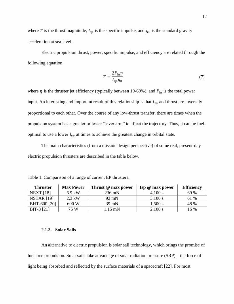
where 𝑇 is the thrust magnitude, 𝐼𝑠𝑝 is the specific impulse, and 𝑔0 is the standard gravity

acceleration at sea level.

Electric propulsion thrust, power, specific impulse, and efficiency are related through the

following equation:

𝑇 =

2𝑃𝑖𝑛𝜂

𝐼𝑠𝑝𝑔0 (7)

where 𝜂 is the thruster jet efficiency (typically between 10-60%), and 𝑃𝑖𝑛 is the total power

input. An interesting and important result of this relationship is that 𝐼𝑠𝑝 and thrust are inversely

proportional to each other. Over the course of any low-thrust transfer, there are times when the

propulsion system has a greater or lesser “lever arm” to affect the trajectory. Thus, it can be fuel-

optimal to use a lower 𝐼𝑠𝑝 at times to achieve the greatest change in orbital state.

The main characteristics (from a mission design perspective) of some real, present-day

electric propulsion thrusters are described in the table below.

Table 1. Comparison of a range of current EP thrusters.

Thruster Max Power Thrust @ max power Isp @ max power Efficiency

NEXT [18] 6.9 kW 236 mN 4,100 s 69 %

NSTAR [19] 2.3 kW 92 mN 3,100 s 61 %

BHT-600 [20] 600 W 39 mN 1,500 s 48 %

BIT-3 [21] 75 W 1.15 mN 2,100 s 16 %

2.1.3. Solar Sails

An alternative to electric propulsion is solar sail technology, which brings the promise of

fuel-free propulsion. Solar sails take advantage of solar radiation pressure (SRP) – the force of

light being absorbed and reflected by the surface materials of a spacecraft [22]. For most

13

spacecraft, SRP is only a minor perturbation. However, a large reflective surface with low mass

has the potential to leverage this effect for substantial acceleration. Since solar sails do not

consume any propellant, they are ideal for perpetually-thrusting mission concepts [9], [23]–[25].

Despite the potential for solar sails in a variety of missions, there has not yet been wide-

spread adoption of the technology. Some challenges are: constrained control authority,

susceptibility to orbiting debris, and complex deployment geometry. This dissertation does not

explicitly use solar sails, but some small changes to the equations of motion and constraints on

thrust would make the same optimization algorithms viable.

2.2. Optimal Control

The optimal control problem can be defined in various ways. We state the problem as:

Minimize the Lagrange performance index

𝐽 = 𝐾[𝒙(𝑡0), 𝒙(𝑡𝑓), 𝑡0, 𝑡𝑓] + ∫ 𝐿[𝒙(𝑡), 𝒖(𝑡), 𝑡]𝑑𝑡

𝑡𝑓

𝑡0

(8)

subject to differential constraints due to the system dynamics

�̇�(𝑡) = 𝒇[𝒙(𝑡), 𝒖(𝑡), 𝑡], (9)

path constraints (such as limiting thrust)

𝒉𝐿 ≤ 𝒉[𝒙(𝑡), 𝒖(𝑡), 𝑡] ≤ 𝒉𝑈 , (10)

and endpoint constraints (such as constraining the initial and final orbits)

𝒆𝐿 ≤ 𝒆[𝒙(𝑡0), 𝒖(𝑡0), 𝒙(𝑡𝑓), 𝒖(𝑡𝑓), 𝑡0, 𝑡𝑓] ≤ 𝒆𝑈 . (11)

For low-thrust trajectory optimization, we find it effective to use an objective function that

consists only of the terms integrated along the path and not the endpoint costs. In this thesis, we

only consider equality constraints in the development of the optimal control policy. The thrust

14

magnitude is inherently an inequality constraint, but it is more easily implemented by directly

limiting thrust in the dynamics function.

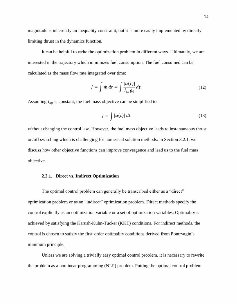
It can be helpful to write the optimization problem in different ways. Ultimately, we are

interested in the trajectory which minimizes fuel consumption. The fuel consumed can be

calculated as the mass flow rate integrated over time:

𝐽 = ∫ �̇� 𝑑𝑡 = ∫

|𝒖(𝑡)|

𝐼𝑠𝑝𝑔0𝑑𝑡. (12)

Assuming 𝐼𝑠𝑝 is constant, the fuel mass objective can be simplified to

𝐽 = ∫|𝒖(𝑡)| 𝑑𝑡 (13)

without changing the control law. However, the fuel mass objective leads to instantaneous thrust

on/off switching which is challenging for numerical solution methods. In Section 3.2.1, we

discuss how other objective functions can improve convergence and lead us to the fuel mass

objective.

2.2.1. Direct vs. Indirect Optimization

The optimal control problem can generally be transcribed either as a “direct”

optimization problem or as an “indirect” optimization problem. Direct methods specify the

control explicitly as an optimization variable or a set of optimization variables. Optimality is

achieved by satisfying the Karush-Kuhn-Tucker (KKT) conditions. For indirect methods, the

control is chosen to satisfy the first-order optimality conditions derived from Pontryagin’s

minimum principle.

Unless we are solving a trivially easy optimal control problem, it is necessary to rewrite

the problem as a nonlinear programming (NLP) problem. Putting the optimal control problem

15

into the format of an NLP is known as transcription, and it is used for direct and indirect

methods. Whatever approach we take to finding an optimal solution, we ultimately solve the

NLP by iteratively solving a series of approximate, linear problems.

When we transcribe the optimal control problem as an NLP, the linearized sub-problems

are always underdetermined using a direct formulation; that is, there are fewer constraints than

optimization variables. A simple way to understand this is that a spacecraft’s state is at least 6-

dimensional, but the control is at most 3-dimensional. We have constraints on the state

dynamics, and we must somehow come up with a set of constraints on the control to ensure that

the objective function is minimized.

For example, consider the two-point boundary value problem with fixed endpoints and

fixed time of flight. Mass is held constant, so the state is 6-dimensional (3 for position, 3 for

velocity). The problem is discretized into N nodes. For the direct formulation, each node contains

9 parameters (3 each for position, velocity, and control). Thus, there are 9𝑁 variables to

optimize. The dynamics constraints are met by forcing state continuity between each pair of

nodes, which gives us 6(𝑁 − 1) dynamics constraints plus 12 additional constraints for the

initial and final states. Subtracting the number of constraints from the number of variables leaves

us with the number of degrees of freedom for the direct formulation:

𝑑𝑜𝑓𝑑𝑖𝑟𝑒𝑐𝑡 = 3𝑁 − 6 (14)

When 𝑁 = 2, we basically have Lambert’s problem. For any 𝑁 > 2, there are infinitely many

possible solutions that satisfy the dynamics constraints. This thesis uses variations of the

sequential quadratic programming (SQP) algorithm, which iteratively solves a linearized version

of the full NLP problem. At each iteration of the SQP algorithm, a quadratic problem solver is

responsible for choosing the feasible solution that minimizes the objective function.

16

For the indirect formulation, each node contains 12 parameters (6 for the state and

another 6 for the adjoints). Control is calculated as a function of the state and adjoints. Then,

there are a total of 12𝑁 variables to optimize. Thanks to Pontryagin’s minimum principle, we

also have additional constraints from the adjoints’ equations of motion. The total number of

constraints is 12(𝑁 − 1) + 12. Simple arithmetic shows us that the indirect formulation has

removed all of the degrees of freedom. Each linearized problem has exactly one solution which

obeys the constraints. Since the problems we deal with in this thesis are nonlinear, it is common

to encounter multiple locally-optimal solutions. If one or more constraints are removed (such as

freeing up one or more of the endpoints or time of flight), then the optimizer must use those

degrees of freedom to minimize the objective function.

2.2.2. Indirect Transcription

Whether using indirect or direct optimization, the first step is to choose an objective

function. There are two objective functions that we are interested in: the integrated control

“energy” and the fuel mass consumed. Both are related to the integrated control effort:

𝑐𝑜𝑠𝑡 = ∫ 𝐿 𝑑𝑡 = ∫|𝒖|𝑝 𝑑𝑡. (15)

When 𝑝 = 2, we have the “minimum energy” problem. With 𝑝 = 1, we have the minimum fuel

problem. In spacecraft trajectory optimization we are generally searching for the minimum fuel

solution, but it is much easier to converge on the minimum energy solution. Leaving 𝑝 as a

variable, we can derive both control laws simultaneously.

Central to the indirect method of optimal control is the introduction of a new set of

variables: the Lagrange multipliers 𝝀, also known as adjoints or costates. The Lagrange

multipliers are used widely to solve constrained optimization problems. In the field of optimal

17

control, we use Pontryagin’s minimum principle to develop a set of constraints on the Lagrange

multipliers which give us criteria for optimal solutions. We use 𝝀(𝑡) to “dualize” the states 𝒙(𝑡).

The states 𝒙(𝑡) are constrained by the equations of motion, so we have an equivalent set of

Lagrange multipliers 𝝀(𝑡) that correspond to the state constraints.

In this work, we use equality constraints 𝒉(𝒙, 𝒖, 𝑡) to enforce the problem dynamics and

to constrain the endpoints. We define the Hamiltonian functional associated with the NLP as

𝐻(𝒙, 𝒖, 𝑡, 𝝀) = 𝐿(𝒙, 𝒖, 𝑡) + 𝝀 ∙ 𝒉(𝒙, 𝒖, 𝑡). (16)

Pontryagin’s minimum principle tells us that the optimal control policy is one which minimizes

the Hamiltonian. Or equivalently:

𝒖∗(𝒙, 𝝀, 𝑡) = arg min𝒖

𝐻(𝒙, 𝝀, 𝒖, 𝑡). (17)

Thus, a necessary condition on the optimal control 𝒖∗ is:

𝜕𝐻

𝜕𝒖│𝒖∗ = 𝟎 (18)

This necessary condition is sufficient for most practical problems. It is generally trivial to choose

the solution 𝒖∗ such that 𝐻 is minimized and not maximized. In some rare cases, we find a

saddle point of 𝐻 with respect to 𝒖. Such cases are referred to as singular arcs because the

control is singular when 𝐻 is minimized only according to the necessary condition. We can

overcome these rare situations by also using the sufficient condition to apply additional

constraints: the matrix [𝜕2𝐻

𝜕𝒖2] must be positive definite.

Pontryagin’s minimum principle gives us dynamics of an optimal control trajectory.

�̇� =

𝜕𝐻∗

𝜕𝝀 (19)

�̇� = −

𝜕𝐻∗

𝜕𝒙 (20)

18

We now have a complete set of dualized dynamics that describe the motion of all trajectories

which locally minimize the integrated cost 𝐿 subject to the constraints 𝒉.

We will now derive the control law for two-body dynamics, assuming constant mass. For

other dynamics, the control law has the same relationship with Lawden’s [26] primer vector 𝝀𝑣

(the costates corresponding to the constraints on the velocity portion of the state). The dynamics

of the costates change for a different dynamical model. For two-body dynamics, the Hamiltonian

is given by

𝐻 = |𝒖|𝑝 + 𝝀𝑇 ([

𝒗

−𝜇

𝑟3𝒓] + [

𝟎3

𝒖]), (21)

where 𝒖 is the control acceleration. This can be simplified to

𝐻 = 𝝀𝑇 [

𝒗

−𝜇

𝑟3𝒓] + |𝒖|(|𝒖|𝑝−1 + 𝝀𝑣

𝑇�̂�). (22)

From above, we know that an optimal control law minimizes the Hamiltonian. Differentiating

the Hamiltonian with respect to control and setting equal to zero yields

𝑝|𝒖|𝑝−1 + 𝝀𝑣 ∙ �̂� = 0. (23)

Looking back at Eq. (22), we can see from inspection that to minimize 𝐻, we should always

choose the control direction �̂� = −�̂�𝑣. The magnitude of control acceleration is found by solving

Eq. (23) for |𝒖|. Now the complete control law as a function of the primer vector 𝝀𝑣 is

𝒖 = − (1

𝑝𝜆𝑣)

1𝑝−1

�̂�𝑣 (24)

for 1 < 𝑝 ≤ 2. If 𝑝 is exactly equal to 1, we make a modification to the control law by inspection

of Eq. (22).

19

𝒖 = {

𝟎3 𝑖𝑓 𝜆𝑣 < 1

−𝑢𝑚𝑎𝑥�̂�𝑣 𝑖𝑓 𝜆𝑣 > 1indeterminate 𝑖𝑓 𝜆𝑣 = 1

(25)

where 𝑢𝑚𝑎𝑥 is the maximum possible control acceleration magnitude. Results in the literature

[27]–[29] and the author’s own experience find that the radius of convergence is much larger

when 𝑝 = 2 than when 𝑝 = 1. Thus, a helpful strategy to solve optimal control problems is to

start with the 𝑝 = 2 solution, then use homotopy to transition to the 𝑝 = 1 solution. Homotopy

methods are discussed more in Section 3.2.1.

We then use Eq. (20) to derive the equations of motion for the adjoints for two-body

dynamics with constant mass:

𝝀�̇� =

𝜇

𝑟3𝝀𝑣 −

3𝜇𝒓 ∙ 𝝀𝑣

𝒓5𝒓 (26)

𝝀�̇� = −𝝀𝑟 . (27)

In general, the equations of motion dictating the evolution of the states and the costates

are known or can be derived, and the initial and final states are dictated by the problem. Given

the additional constraints from Pontryagin’s minimum principle, we can restate the optimal

control problem as: Find the initial costates which, when propagated with the states according to

the control law, result in a solution to the two-point boundary value problem.

A common argument against indirect methods is that there is no good way to guess the

costates. One way to overcome this limitation is to guess the initial costates randomly, many

times, and propagate each forward to see if it reaches the final state. Reference [30] applied this

successfully to find a vast array of solutions to a few particular 2PBVP’s in the Earth-Moon

problem. The downside to this approach is the enormous computer resources required. We

demonstrate in this thesis that we can reliably converge on optimal transfers in two-body and

three-body dynamics using minimal initial information. We then make a larger contribution by

20

developing an algorithm for training a neural network to map the relationship between states and

adjoints in a localized area of the solution space.

2.2.3. Direct Transcription

The other broad category of solution methods used in this thesis is the direct approach,

where we use any of a number of numerical optimization techniques to solve an NLP problem.

The term “direct transcription” is used very generally to describe any means of rewriting an

optimal control problem into a NLP problem. Betts has written extensively on the topic and

demonstrated various related optimization strategies for a wide array of problem types [7], [31]–

[34]. Many other authors have also contributed to the subject; some notable contributions come

from Gill, Murray, Saunders and Wright [35], [36], Enright and Conway [37], Hargraves [38],

Ross [39], and Rao [40]. Three transcription methods are used in this research: single shooting,

multiple shooting, and collocation. These transcription methods are described in Section 2.2.5.

A great advantage to direct optimization is that all the hard work is done behind the

scenes by the NLP solver. The user can simply provide the optimization problem in the simple

format below. In this case, we set up the problem such that all optimization variables are treated

the same (all states, controls, etc. are concatenated into one vector 𝒙).

minimize: 𝐽(𝒙) (28)

subject to: 𝒉(𝒙) = 𝟎

𝒈(𝒙) ≤ 𝟎

(29)

The objective 𝐽(𝒙), equality constraints 𝒉(𝒙), and inequality constraints 𝒈(𝒙) are all general

nonlinear functions. Any smooth optimization problem with a scalar objective can be described

in these terms. The danger with this convenience is that the user may be unaware if the problem

is poorly formulated; it is not obvious to the user why some problems fail.

21

The field of nonlinear programming is vast, and a thorough description of all solution

methods is beyond the scope of this thesis. The sequential quadratic programming (SQP)

algorithm has been shown to be effective at solving the NLP problems arising from optimal

control [33], [41]. Early work in this thesis compared the SQP and interior-point algorithms as

implemented in MATLAB Optimization Toolbox. Both methods yielded comparable results,

with the SQP algorithm tending to converge slightly more quickly. Based on the results in the

literature and the author’s anecdotal evidence, the SQP algorithm was used going forward.

There are many ways the SQP algorithm can be implemented; for specific examples and

more detail, the reader is referred to references [36], [42]. The general principles of the SQP

algorithm are described below.

2.2.4. Sequential Quadratic Programming

Since it is, in general, hard or impossible to analytically solve a nonlinear problem, we

need to convert the problem into some form that is possible to solve. The Sequential Quadratic

Programming (SQP) algorithm is a robust option. The basic concept is to solve a series of

quadratic sub-problems, each of which approximate the nonlinear problem at the current iteration

[36], [43].

While NLP solvers present a simple user interface allowing any kind of smooth objective

and constraints, the math used internally in the SQP algorithm is quite similar to the math used in

indirect optimal control. Similar to minimizing the Hamiltonian 𝐻 from Section 2.2.2, we now

seek the solution which minimizes the Lagrangian ℒ given by:

ℒ(𝒙, 𝝀) = 𝐽(𝒙) + 𝝀 ∙ 𝒉(𝒙). (30)

where 𝜆 is, again, a set of Lagrange multipliers. These adjoints usually remain hidden to the user

when solving a problem with the direct method, but they are equivalent to the adjoints introduced

22

in Pontryagin’s minimum principle. Leaving off the inequality constraints for simplicity, the

optimization problem is now described as

minimize: ℒ(𝒙, 𝝀) = 𝐽(𝒙) + 𝝀 ∙ 𝒉(𝒙) (31)

subject to: 𝒉(𝒙) = 𝟎. (32)

Since we do not have any means to easily solve general nonlinear equations, we approximate the

NLP problem as a quadratic programming (QP) problem at each iteration. We can construct an

approximate model of the Lagrangian with a 2-term Taylor series expansion about the state 𝒙𝑘:

ℒ(𝒙, 𝝀) ≈ ℒ(𝒙𝑘 , 𝝀𝑘) + ∇ℒ(𝒙𝑘 , 𝝀𝑘)𝑇Δ𝒙 +

1

2Δ𝒙𝑇[Ηℒ(𝒙𝑘 , 𝝀𝑘)]Δ𝒙 (33)

where Ηℒ(𝒙𝑘 , 𝝀𝑘) is the Hessian of the Lagrangian evaluated at state 𝒙𝑘 and adjoints 𝝀𝑘. When

ℒ is a large, messy function (as it frequently comes out to be in optimal control), it is

computationally expensive to generate the Hessian matrix. Some NLP solvers approximate the

Hessian matrix to improve convergence compared to using only a 1-term Taylor series expansion

[36], [42].

Ideally, we would like to use a 2-term Taylor series expansion of the constraints in

addition to the 2-term expansion of the Lagrangian. However, there are no practical methods to

directly solve multivariate problems with quadratic equality constraints. Quadratic programming

(QP) is a well-defined class of optimization problems for which many well-established, high-

performance solvers exist. A QP problem consists of some set of the following: linear equality

constraints; linear objective; and quadratic objective. Second-order conic programming (SOCP)

is closely related to QP, with the distinction that QP only allows inequality constraints to be up to

linear, while SOCP allows inequality constraints to be up to quadratic. Since we have neglected

inequality constraints here, we have a QP problem.

23

At this point, we have introduced a new set of variables with the Lagrange multipliers 𝝀,

but we have not yet introduced any new constraints. In addition to the constraints 𝒉(𝒙) (used in

optimal control to enforce the equations of motion), we can come up with a set of constraints on

𝝀 from the 1-term Taylor series expansion of the Lagrangian. We know from basic calculus that

the first derivative of a function with respect to its inputs must be zero at a maximum or

minimum. Thus, we have the Karush-Kuhn-Tucker (KKT) conditions [44]:

∇ℒ(𝒙, 𝝀) = ∇𝐽(𝒙) + ∇𝒉(𝒙) ∙ 𝝀 = 𝟎. (34)

Finally, the quadratic problem at each iteration of the SQP algorithm is constructed as follows:

minimize: 𝛻ℒ(𝒙𝑘 , 𝝀𝑘 , 𝝁𝑘) ∙ Δ𝒙 + 1

2Δ𝒙 ∙ 𝐻ℒ(𝒙𝑘 , 𝝀𝑘) ∙ Δ𝒙 (35)

subject to: 𝒉(𝒙𝑘) + 𝛻𝒉(𝒙𝑘) ∙ Δ𝒙 = 𝟎

∇𝐽(𝒙𝑘) + ∇𝒉(𝒙𝑘) ∙ 𝝀 = 𝟎. (36)

Note that this is just one of many similar ways to construct the approximate QP problem. After

each iteration, the optimization variables are updated as

𝒙𝑘+1 = 𝒙𝑘 + Δ𝒙 (37)

When the problem is fully solved (if the states and control are parameterized the same

way), the solution (𝒙∗, 𝝀∗) should be identically the same as the solution from indirect optimal

control, with the exception that 𝝀∗ may be scaled by some scalar. The scale difference in 𝝀∗

arises because the �̇� dynamics from Pontryagin’s minimum principle are scale-invariant for our

problems.

From the description in this section, the author hopes to make it clear that “direct” and

“indirect” formulations of the optimal control problem are really just different ways of deriving a

set of constraints on the Lagrange multipliers 𝝀 used to enforce the problem constraints. Note

that the indirect formulation uses 𝝀𝑖𝑛𝑑𝑖𝑟𝑒𝑐𝑡(𝑡𝑗), defined in practice at some set of discrete times

24

𝑡𝑗. The direct formulation defines 𝝀𝑑𝑖𝑟𝑒𝑐𝑡 as a single, large vector. The two may be equated

through the pseudocode

𝝀𝑖𝑛𝑑𝑖𝑟𝑒𝑐𝑡(𝑡𝑗) = 𝑟𝑒𝑠ℎ𝑎𝑝𝑒(𝝀𝑑𝑖𝑟𝑒𝑐𝑡 , 𝑛, 𝑁), (38)

where 𝑛 is the length of the state vector (6 in this thesis) and 𝑁 is the number of nodes at which

the state and adjoints are defined. Either method may be more numerically stable for a particular

optimal control problem. In practice, the direct formulation tends to be more robust to a poor

initial guess, while the indirect formulation tends to be better able to converge to tight tolerances.

2.2.5. Numerical Approaches

Some simple problems may be solved by hand using Pontryagin’s principle and the

related math developed by earlier mathematicians. However, for practical astrodynamics

problems, it is generally impossible to do this. In practice, it is necessary to transcribe the

optimal control problem into a nonlinear programming (NLP) problem.

Some of the most widely-used NLP solvers include SNOPT [36], IPOPT [45], MATLAB

Optimization Toolbox, and KNITRO. Some examples of these NLP solvers in trajectory

optimization include: NASA Goddard’s GMAT (General Mission Analysis Tool) and its CSALT

collocation tool; PSOPT (PseudoSpectral OPTimization) open-source collocation tool [46]–[48];

NASA Goddard’s EMTG (Evolutionary Mission Trajectory Generator) [49]; NASA Johnson’s

Copernicus Trajectory Design and Optimization System; and NASA JPL’s MALTO (Mission

Analysis Low Thrust Optimizer) [50]. CSALT, EMTG, Copernicus, and MALTO all use the

SNOPT solver, which implements the SQP algorithm. PSOPT uses the IPOPT solver, which

implements the interior-point algorithm.

25

While these solvers are powerful and adept at solving a wide array of problems, we find

in this thesis that they can be very slow for low-thrust trajectory optimization – particularly as

the problem size grows or as the linear assumptions internal to the optimizer break down. With

the exception of IPOPT (which is open-source), high-performance NLP solvers are generally

closed-source and each is set up as an “engineering black box”. When the algorithm encounters

difficulties with an optimization problem, there is very little the user can do to improve the

situation. Understanding the transcription methods described below is important for mission

designers so that it becomes more clear why their optimization problems are difficult.

2.2.5.1. Single Shooting

The namesake example for single shooting is the classic problem of aiming a cannon at a

target. The cannon can be adjusted up or down, left or right. The left/right aiming is linear with

respect to the initial condition (assuming low wind speeds), so the operator can simply point the

cannon at the target. Up/down aiming has a nonlinear relationship with the initial condition.

Once shot, the cannonball is acted on by some nonlinear dynamics (gravity, drag, etc.) until it

collides with the ground. The operator then adjusts the aim and fires again, refining the aim point

until the target is achieved.

When used in astrodynamics, single shooting is typically used in either a direct

formulation with a single impulsive maneuver at the start (the cannon “bang”), or an indirect

formulation where the optimization variables consist of the adjoints at the initial or final time.

Single shooting has the advantage of being very fast to iterate because there are only a small

number of variables. Evaluating a candidate trajectory simply requires numerically integrating

the initial state forward in time. However, the method is limited in its practical use because of the

26

extreme sensitivity of the end state with respect to the beginning state for long trajectories. A

conceptual drawing of single shooting is shown in Figure 5.

Figure 5. Conceptual sketch of single shooting.

Single shooting generally consists of iteratively using the linear Taylor series expansion

of the end state as a function of the initial conditions.

𝒙𝑓 ≈ 𝒙𝑓

∗ +𝜕𝒙𝑓

𝜕𝒙0∙ Δ𝒙0 (39)

Solving for Δ𝒙0 yields an update to the initial condition:

Δ𝒙0 = [

𝜕𝒙𝑓

𝜕𝒙0]

−1

∙ (𝒙𝑓 − 𝒙𝑓∗). (40)

If the system can reasonably be approximated by a linear approximation, then single shooting

can converge quickly. The method struggles with trajectory optimization problems that involve

close flybys of massive bodies, as the flyby invalidates the linearity assumption.

2.2.5.2. Multiple Shooting

Multiple shooting extends the core concept of single shooting, alleviating the main

limitation of single shooting by breaking the trajectory up into multiple segments. While the

27

relationship from 𝒙0 to 𝒙𝑓 might be highly nonlinear, the relationship from 𝒙0 to 𝒙1 can be

arbitrarily close to linear, depending on the number of nodes used. Figure 6 shows a conceptual

sketch of multiple shooting, for comparison with single shooting.

Figure 6. Conceptual sketch of multiple shooting.

2.2.5.3. Sims-Flanagan and FBLT

The Sims-Flanagan transcription [50], [51] is a popular and well-proven variant of direct

transcription, based on the CATO algorithm [52] and built into the MALTO tool [53]. In the

Sims-Flanagan transcription, the dynamics are modeled as ballistic (no thrust) between impulses,

and each impulse is constrained to be at most equal to the accumulated Δ𝑉 that would be

achieved by constant thrust over the corresponding trajectory segment. The optimization

variables consist of:

• State 𝒙𝒊 at a small number of control nodes (for interplanetary problems, the

control nodes could be at planetary encounters)

28

• Impulsive control 𝚫𝑽𝒊,𝒋 at a number of segments (typically 30-100) between each

control node.

The constraints consist of:

• Match point error 𝜹𝑿𝒊 between each control node

• Thrust magnitude, implemented by limiting the size of each 𝚫𝑽𝒊,𝒋.

A slight change to the Sims-Flanagan transcription is the so-called FBLT (Finite Burn

Low Thrust) transcription. The FBLT transcription characterizes a trajectory as a series of

segments with continuous thrust, with thrust magnitude and direction fixed per segment [54].

Apart from describing the maneuver differently, this transcription is identical to Sims-Flanagan.

The Sims-Flanagan and FBLT transcriptions were designed specifically for solving the

interplanetary low-thrust transfer problem, and their assumptions limit their applicability to

different dynamics.

2.2.5.4. Collocation

The basic principle of collocation is to represent an ordinary differential equation with

some continuous function which obeys the differential equations of motion at a set of nodes.

Collocation transcribes an optimal control problem to an NLP problem which can be solved by

any industry-standard NLP software [55]. A variety of collocation-based methods exist,

distinguished by the node spacing and the choice of basis functions. Global methods such as

Legendre pseudospectral collocation use a single high-order Lagrange basis polynomial to

approximate the entire trajectory. Local methods such as Hermite-Simpson collocation use many

low-order polynomials to fit the trajectory in parts [56].

A helpful way to think of collocation is through a comparison to implicit numerical

integration schemes. When propagating a system with known forces, information about the

29

current state and, possibly, the state at previous integration steps is used to calculate the state at

some time in the future. In collocation, rather than propagating a known initial state through

known forces, the states and controls are optimization parameters subject to constraints. In order

to find a solution which obeys the differential equations of motion, a defect is calculated at or

between each node. Reference [57] has an excellent description of collocation.

Figure 7. Conceptual sketch of collocation.

Collocation has been used by several researchers to solve optimal control problems in N-

body gravity fields [10], [25], [32], [34], [58]–[60]. It shows great promise as a technology, but

there is no magic bullet for optimal control. Collocation by definition uses a large number of

optimization variables (hundreds for a small problem, up to hundreds of thousands for a large

problem), which can make it very slow to run. Although collocation solves the problem of

nonlinearity between neighboring nodes, it still has the problem of nonlinearity from one

endpoint to the other, or from one flyby to another.

In this research, three collocation methods have been used: Legendre pseudospectral on

Legendre-Gauss-Lobatto nodes with the open source optimal control package PSOPT

30

(PseudoSpectral OPTimal control) [46]; Legendre pseudospectral on Legendre-Gauss-Radau

nodes with prototype software in development at Goddard Space Flight Center for use in GMAT

(General Mission Analysis Tool); and the author’s own implementation of Hermite-Simpson

collocation. The differences between them consist mainly in the amount of a trajectory

represented with a single polynomial, the polynomial degree used, and the type of polynomial.

Regardless of the type of collocation, the purpose is to transcribe the optimal control problem

into an NLP problem which can be passed to an NLP solver. The solver attempts to minimize the

cost function while not violating the constraints more than an acceptable amount.

The most basic implementation of pseudospectral collocation uses a single phase to

represent the whole trajectory, so an Nth order polynomial is required to represent a trajectory

with N collocation points. While this approach works for some problems, it is easy to think of

cases where we would run into problems. For example, if an Earth-centric trajectory has a flyby

of the Moon in the middle, the rapidly-changing dynamics near the flyby will be captured

extremely poorly by the global polynomial. If we increase the number of nodes until there are

sufficiently many to represent the flyby accurately, we will end up with too many nodes during

the rest of the trajectory. A simple workaround is to borrow some ideas from multiple shooting:

break the problem into multiple phases, where the number of nodes can be adjusted for each

phase independently.

Liu, Hager, and Rao [61] take this idea further with what they refer to as “hp mesh

refinement”. In the mesh refinement stage, the algorithm has a choice to either increase the

number of phases or the number of nodes (equivalently, polynomial degree) in each phase. They

develop a method for automatically refining the number of phases in addition to refining the

31

number of nodes in each phase, using Legendre-Gauss-Radau nodes. This variation is

implemented in the GMAT prototype collocation tool.

Collocation methods can generate high-quality solutions to relatively simple problems in

seconds to minutes. However, collocation can be ineffective for problems involving multiple

orbital revolutions or flybys of Earth or Moon. Current NLP algorithms have a single-thread

execution bottleneck, and the large number of variables used in collocation can cause

unnecessary slowdowns.

2.3. Methods of Differentiation

When solving optimization problems, we naturally are faced with taking many

derivatives of nonlinear, problem-dependent functions. For example, to construct a linear

approximation of the nonlinear constraints, we must come up with the (sparse) Jacobian matrix

J =

𝜕𝒄

𝜕𝑿 (41)

where 𝒄 is the vector of all the constraints and 𝑿 is the vector of all the optimization variables.

The number of derivatives grows as a function of the size of the problem and the sparsity of the

Jacobian. Constructing the Jacobian is typically a major fraction of the total computational cost.

The accuracy of partial derivatives also has implications on the convergence of optimization

methods; a solver given inaccurate derivatives will have trouble converging. Therefore, it is

important to compute the derivatives efficiently and accurately.

Whenever possible, the “best” derivatives come from analytically differentiating by hand.

A capable mathematician can arrive at an efficient way to compute the gradients of the “messy”

vector functions that arise in optimal control. Assuming the mathematician has not made any

mistakes, the analytical solution will have perfect accuracy. In some cases, it is not possible to

32

derive an analytical solution. Symbolic manipulation software such as Maple, Mathematica,

EES, or MATLAB Symbolic Toolbox can produce analytical derivative functions, but they tend

to have trouble simplifying vector calculus expressions. When the equations involved get

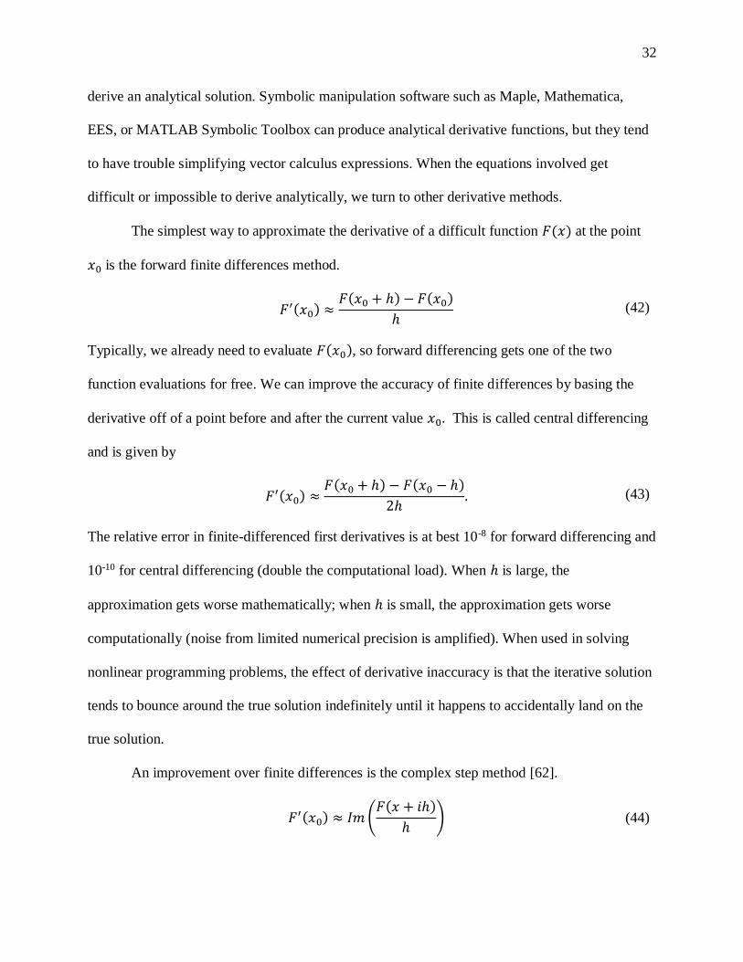
difficult or impossible to derive analytically, we turn to other derivative methods.

The simplest way to approximate the derivative of a difficult function 𝐹(𝑥) at the point

𝑥0 is the forward finite differences method.

𝐹′(𝑥0) ≈

𝐹(𝑥0 + ℎ) − 𝐹(𝑥0)

ℎ (42)

Typically, we already need to evaluate 𝐹(𝑥0), so forward differencing gets one of the two

function evaluations for free. We can improve the accuracy of finite differences by basing the

derivative off of a point before and after the current value 𝑥0. This is called central differencing

and is given by

𝐹′(𝑥0) ≈

𝐹(𝑥0 + ℎ) − 𝐹(𝑥0 − ℎ)

2ℎ. (43)

The relative error in finite-differenced first derivatives is at best 10-8 for forward differencing and

10-10 for central differencing (double the computational load). When ℎ is large, the

approximation gets worse mathematically; when ℎ is small, the approximation gets worse

computationally (noise from limited numerical precision is amplified). When used in solving

nonlinear programming problems, the effect of derivative inaccuracy is that the iterative solution

tends to bounce around the true solution indefinitely until it happens to accidentally land on the

true solution.

An improvement over finite differences is the complex step method [62].

𝐹′(𝑥0) ≈ 𝐼𝑚 (

𝐹(𝑥 + 𝑖ℎ)

ℎ) (44)

33

When ℎ is chosen as 10-8 or smaller, the first derivative is accurate to numerical precision. This

method does not extend well to higher derivatives. For comparison with the multicomplex and

dual numbers methods described below, it is helpful to think of the complex numbers as a

limited extension of the real numbers. Although it may seem trivial to state, the complex

numbers consist of the set ℂ composed of a real dimension and a non-real dimension.

ℂ ≔ {𝑎 + 𝑏𝑖 / 𝑥, 𝑦 ∈ ℝ} (45)

Here, 𝑎 is the real component and 𝑏 is the imaginary component. The main property of the

element 𝑖 is that 𝑖2 = −1.

Lantoine [63] presented the multicomplex numbers as a way to compute derivatives of

any order that are accurate to machine precision. Multicomplex numbers are a multi-dimensional

generalization of complex numbers. The multicomplex method is similar in concept and practice

to the use of dual or hyper-dual numbers for automatic differentiation. Out of convenience, the

dual numbers are used in this thesis (implemented via operator overloading in the DualNumbers

and ForwardDiff [64] packages for the Julia programming language). The dual numbers likewise

consist of a real dimension and another dimension, in this case referred to as the epsilon

dimension.

𝒟 ≔ {𝑎 + 𝑏𝜖 / 𝑥, 𝑦 ∈ ℝ} (46)

The main property of the dual element 𝜖 is that 𝜖2 = 0. For us, the useful property of dual

numbers is that we can evaluate any function 𝐹(𝑥) and get the derivative with respect to 𝑥 for

free.

𝐹(𝑥 + 𝜖ℎ) = 𝐹(𝑥) + ℎ𝐹′(𝑥)𝜖 (47)

𝐹′(𝑥)𝜖 =

𝐹(𝑥 + 𝜖ℎ) − 𝐹(𝑥)

ℎ (48)

34

Since we get the derivative “automatically” when following the rules of dual number math, its

use is typically referred to as “automatic differentiation.” For simplicity, we choose ℎ = 1. We

can take an arbitrary number of derivatives using hyper-dual numbers, which extend the same

concept into higher dimensions. All derivatives are computed perfectly to numerical precision.

As implemented in this thesis, automatic differentiation is comparable in computer time

to the method of finite differences. In some instances, it was up to ~2x faster to use finite

differences, and in other cases, it was up to ~2x faster to use automatic differentiation. The

advantage clearly goes to automatic differentiation because of the accuracy improvement.

Others have used automatic differentiation in optimal control, but the practice does not

seem to be widespread. The open-source pseudospectral collocation tool PSOPT implements the

ADIFOR automatic differentiation package for Fortran [46], [65]. Automatic differentiation

packages exist for most programming languages, including Julia, Python, MATLAB, C, C++,

Fortran, and Java. There are many ways to implement automatic differentiation, and some can be

much slower than finite differences. It seems that the astrodynamics community is not fully

aware of the benefits of automatic differentiation. For some applications, finite differences are

“good enough”. In the Julia language, automatic differentiation is painless and fast, and we

commend its use in trajectory optimization.

2.4. Neural Networks

From an engineering perspective, neural networks (NNs) can be thought of as a form of

nonlinear regression. Although not precisely accurate, thinking in this way is conceptually sound

for the configuration used in this research: a feedforward neural network. The basic idea of an

NN is inspired by the functioning of a biological brain. The network consists of a number of

“neurons” which each produce an activation response as a function of the inputs from other

35

connected neurons [66], [67]. A feedforward NN is organized as shown in Figure 8. Within the

network, each neuron is modeled as shown in Figure 9.

Figure 8. Schematic drawing of a feedforward neural network. The outputs of each layer are the

inputs to the subsequent layer.

Figure 9. Schematic drawing of a single neuron in a neural network.

36

The function 𝜙(𝑧) can be any sigmoid function (any function with an “S”-shaped curve).

The logistic function is a special case of the sigmoid functions and is given by:

𝑆(𝑧) =1

1 + 𝑒−𝑥 (49)

The tanh(𝑧) function is used in this research, which is related to the logistic function. The

logistic function maps output to [0, +1], while the tanh(𝑧) function maps output to [-1, +1].

𝜙(𝑧) = 𝑡𝑎𝑛ℎ 𝑧 =2

1 + 𝑒−2𝑧− 1 (50)

Either of these functions can be used equivalently in a neural network, with the appropriate

change in network weights. The tanh(𝑧) function is drawn below for reference.

Figure 10. Plot of the function 𝜙(𝑧) = tanh(𝑧).

A helpful way to think of an NN is that each layer transforms the outputs of the previous

layer by shifting, scaling, and remapping to be in [-1, +1]. With enough neurons in even a single

hidden layer (and an arbitrarily large number of training samples), a neural network can

represent any arbitrarily complex relationship between inputs and outputs [66]. In practice, an

37

NN that is too “deep” relative to the number of training samples will tend to over-fit the training

data and generalize poorly to new data. Thus, the engineer is responsible for choosing an

appropriate size of neural network.

As a toy problem, we can use an NN to “learn” the function

𝑦 = sin(2𝑥) + 𝑥2. (51)

We generate “training samples” by evaluating the function at 20 values of 𝑥, spaced uniformly in

the range [-3, +3]. We then “train” the network with 70% of the samples (drawn randomly from

the training set) and use the remaining samples for validation. We use the MATLAB 2018a

Neural Network Toolbox. Results of this simple example are shown in Figure 11.

Figure 11. Example of NN as curve fitting. The true function is closely overlapped by the NN

model with 5 neurons. The true function is: 𝑦 = sin(2𝑥) + 𝑥2.

For an NN with scalar input/output and only 1 hidden layer, the number of parameters to

tune in the NN training is 3𝑁 + 1, where 𝑁 is the number of neurons. Since we only have 20

38

training samples, the training will be degenerate for 𝑁 > 6. With small 𝑁, the network captures

the broad pattern of the output, but not the details. With large 𝑁, the network over-fits and

exhibits “ringing” similar to Gibbs’ phenomena for polynomial curve fitting. Notice that with

𝑁 = 20, most of the training samples are captured perfectly, but a few are missed. This behavior

results from using only 70% of the training samples for training. The remaining samples are used

for validation, which provides a check on the NN accuracy.

For a given number of training samples available, there always exists some middle

ground where the network can extract the most information out of the training data without over-

fitting. Here, 𝑁 = 5 works well. Of course, this simple example is not a good use of an NN. The

strength of NNs is not that they can learn simple functions but that they can learn incredibly

complex ones that cannot be described well by any other known method.

NNs are used widely in a variety of fields. To date, the most widespread applications

have been computer vision [68] and audio recognition [67], [69]. For these applications, the NN

is used for classification as opposed to regression. The principle difference between

classification and regression is that the final layer is modified to output discrete values for

classification (for example, to categorize images as “dog”, “cat”, or “umbrella”) and continuous

values for regression [66].

Developments in the last few years have seen NNs emerge as a powerful technique to

approach many problems. Some example applications of NNs in the aerospace literature are:

• Mapping state and control at time 𝒕𝒊 to time 𝒕𝒊+𝟏 within a collocation scheme, as an

approximation to costly numerical integration [70].

• Mapping initial and final asteroid orbits to the fuel mass required to perform an optimal

low-thrust transfer [71].

39

• Mapping state to control for an optimal low-thrust interplanetary transfer [72], [73].

• Mapping camera visual input to a state estimate for a rocket landing [72], [74].

Neural network training is a broad subject that will not be described in detail in this

thesis. In general terms, the NN parameters are optimized by randomly choosing initial

parameter values, propagating the training sample inputs through the network, checking the error

with the training sample outputs, then back-solving for the weights which minimize the error

between the NN output and the training sample outputs. There is a wide array of training

algorithms available. For more information, the reader is directed to reference [66]. In this thesis,

the Levenberg-Marquardt (for small NNs) and scaled conjugate gradient (for large NNs)

algorithms are used, as implemented in the MATLAB 2018a Neural Network Toolbox.

40

3. Efficient Formulation of Multiple Shooting

In this chapter, we show how the low-thrust trajectory optimization problem can be

solved practically by a few numerical methods. First, we show a direct multiple shooting

method. We find that fixed-step numerical integration is effective for handling poor initial

guesses. The concept of mesh refinement is borrowed from collocation and applied here to

ensure accuracy and numerical stability. Then, we show indirect single shooting as a fast, but

less robust solution method. Finally, we introduce an effective implementation of indirect

multiple shooting, which has some strengths of both previous methods. In all cases, we begin

with a less-sensitive objective function: “minimum energy” for the direct method, and a sigmoid-

smoothed switching function for the indirect methods. Homotopy is used to transition from the

smooth control law to a fuel-optimal control law with a “bang-coast-bang” switching structure.

Initial guess methods are discussed. With a combination of direct and indirect multiple shooting,

we demonstrate an effective path to finding a solution, even given no knowledge of the solution

space.

The tools presented here overcome a few challenges endemic to low-thrust trajectory

optimization: initial guess generation for unintuitive trajectories, linearization breakdown, and

changing dynamics due to flybys. We demonstrate methods of initial guess generation and

robustness to poor initial guesses. We find that linearized approximations are sufficient for the

dynamics constraints but not for the endpoints constraints, and we develop an efficient way to

incorporate a quadratic approximation of endpoints constrained to lie on three-body orbits or

trajectories. We also combine elements of multiple shooting and collocation for accuracy and

performance.

41

Some numerical considerations apply to any trajectory optimization problem. The most

important (and easiest to address) is scaling. An effective rule of thumb is to scale all variables to

be on the order of 1. In this thesis, interplanetary problems scale position terms by 1

astronomical unit (AU), velocity terms by 30 km/s (approximately the speed of Earth around

Sun), position costate terms by 10-7 (found empirically), and velocity costate terms by 0.7 (found

empirically). Problems in the CR3B dynamics use the traditional dimensionless units, which are

naturally scaled well.

By using a combination of direct and indirect multiple shooting, we can find good

solutions to problems where engineering intuition fails. The following diagram summarizes the

approaches found to be effective in this thesis.

Figure 12. Diagram of methods to arrive at the fuel optimal solution.

42

3.1. Direct Multiple Shooting

Direct multiple shooting breaks a trajectory down into a set of N nodes, where each node

has position, velocity, and control. The optimal control problem is posed as a nonlinear

programming (NLP) problem, then solved with variations of the sequential quadratic

programming (SQP) algorithm. For each iteration of the SQP algorithm, the relative time

between each node is fixed, though the total time of flight is an optimization variable. For each

pair of nodes, the state is propagated forward halfway from the first and backward halfway from

the second. Continuous thrust is held constant for each node. The defect 𝒉 in state at the

midpoint is constrained to be zero.

The Jacobian of the defect constraints with respect to all optimization variables is used to

linearize the dynamics constraints. The size of the Jacobian matrix grows with 𝑁2, where 𝑁 is

the number of nodes used. However, the number of nonzero elements grows with 𝑁. Since the

Jacobian is sparse, we save computation time by computing only the partials that may be

nonzero.

If the endpoints (initial and final nodes) and time of flight are held constant, then the

dynamics constraints and objective function alone are enough to find optimal solutions. Adding

these few extra variables to the optimization problem significantly increases its complexity, so a

full section is devoted to it below.

We use two methods to solve trajectory optimization problems with direct multiple

shooting: a two-stage differential corrector, and a simplified version of the SQP algorithm. Both

use a similar approach to transcribe the optimal control problem into an NLP problem, but

different methods to solve the NLP problem. The two-stage differential corrector uses many

impulsive maneuvers to approximate continuous low-thrust control, and the simplified SQP

43

algorithm uses continuous control with discrete changes in control direction (coined “FBLT” by

some authors).

3.1.1. Two-Stage Differential Corrector

Here we implement a two-stage differential corrector as a way to find the minimum

energy solution to the two-point boundary value problem. By using two stages, we separate the

problem into two parts: the inner stage handles feasibility, while the outer stage handles

optimality. The inner stage chooses the impulsive control to perfectly follow the dynamics, and

the outer stage chooses the position vectors to minimize the required control effort.

Two-stage differential correctors have been used previously in astrodynamics to find

periodic orbits in the CR3BP, find ballistic transfers between libration point orbits, and correct

low-fidelity simulations into high-fidelity ephemeris models [15]. The traditional implementation

does not allow thrust, so the velocity and position are required to match at each node. When

using electric propulsion, we do have some limited thrust available. Position is required to match

at each node, and the discontinuity in velocity represents a small impulsive maneuver. If these

maneuvers are small enough and close enough in time, a trajectory modeled in this way can

approximate a continuous-thrust maneuver.

In this work, we use the simplest optimization strategy possible: an ordinary least squares

solver. In the inner loop, a shooting method is implemented to find the velocities at each

endpoint, given the positions and the time of flight between them. For two-body point-mass

dynamics, this is equivalent to solving Lambert’s problem. For any arbitrary force model, a

simple algorithm is implemented as follows.

For the initial guess, assume that the trajectory follows a straight line between position

vector 𝒓𝑖 at node 𝑖 and position vector 𝒓𝑖+1 at node 𝑖 + 1. Then, the velocity guess at node 𝑖 is:

44

𝒗𝑖

𝑔𝑢𝑒𝑠𝑠=

(𝒓𝑖+1𝑔𝑖𝑣𝑒𝑛

− 𝒓𝑖𝑔𝑖𝑣𝑒𝑛

)

𝑡𝑖+1 − 𝑡𝑖. (52)

The state defined by 𝒓𝑖 , 𝒗𝑖 is propagated via numerical integration from time 𝑡𝑖 to time 𝑡𝑖+1,

using a fixed-step integrator. A fixed-step integrator is chosen over an adaptive step integrator

because a variable step integrator will become very slow if an intermediate solution comes near a

singularity. Although a fixed-step integrator is inaccurate near a singularity, we generally want to

avoid flying a spacecraft too close to any massive body anyway. Once a low-fidelity solution has

been found, we can simply add more nodes where needed to meet integration accuracy

requirements. This helps the algorithm survive the first few iterations of a poor initial guess. For

the differential corrector method, partial derivatives are computed via finite differencing. We

find that finite differencing with a variable-step numerical integrator introduces noise that

renders the derivatives inaccurate. Using a fixed-step integrator with finite differencing ensures

consistent derivatives.

The position error to be removed is then given by:

𝛿𝒓𝑖+1 = 𝒓𝑖+1𝑔𝑖𝑣𝑒𝑛

− 𝒓𝑖+1𝑝𝑟𝑜𝑝. (53)

The Jacobian [𝐽𝑖𝑛𝑛𝑒𝑟] is defined as:

[𝐽𝑖𝑛𝑛𝑒𝑟] =

𝜕(𝛿𝒓𝑖+1)

𝜕𝒗𝑖. (54)

The least squares update to velocity is then:

𝒗𝑖 = 𝒗𝑖𝑔𝑢𝑒𝑠𝑠

− [𝐽𝑖𝑛𝑛𝑒𝑟]−1𝛿𝒓𝑖+1. (55)

Once the velocity departing and arriving at each node has been found in the inner loop, the

impulsive 𝛥𝒗𝑖 is simply the difference between the velocity going into node 𝑖 and the velocity

leaving node 𝑖. Control is not constrained in this approach, so 𝛿𝒓𝑖+1 converges to numerical

45

precision within a few iterations. Each pair of adjacent nodes in the inner loop can be considered

completely independent of the others.

For the outer loop, finite differencing is again used to construct the Jacobian matrix.

Now, the Jacobian is the partial derivative of each 𝛥𝒗𝑖 element with respect to each position 𝒓𝑖

element. The vector 𝑹 is composed of all the position vectors 𝒓𝑖 , 2 ≤ 𝑖 ≤ (𝑁 − 1), and the

vector 𝑽 is composed of all the impulsive maneuvers 𝛥𝒗𝑖 , 1 ≤ 𝑖 ≤ 𝑁. The outer stage Jacobian is

then

[𝐽𝑜𝑢𝑡𝑒𝑟] =

𝜕𝑽

𝜕𝑹. (56)

For the two-stage differential corrector, the initial and final position vectors are held fixed, and

time of flight is also fixed. The outer loop Jacobian is a sparse matrix; each position vector 𝒓𝑖

influences three 𝛥𝒗 vectors: 𝛥𝒗𝑖−1, 𝛥𝒗𝑖 , and 𝛥𝒗𝑖+1. The size of the outer loop Jacobian is 3𝑁

rows (corresponding to 𝑽) by 3(𝑁 − 2) columns (corresponding to 𝑹).

The “least squares” solution to any problem gets its name from the fact that it minimizes

the sum of the squares of the quantities of interest. At each iteration of the outer loop, the

quantity

∑|Δ𝒗𝑖|2

𝑁

𝑖=1

= ∑ 𝑉𝑖2

3𝑁

𝑖=1

(57)

is minimized. At each iteration, this is done by solving a linear approximation of the cost as a

function of the position vectors:

𝑽 ≈

𝜕𝑽

𝜕𝑹∙ 𝑹 = 𝐽 ∙ 𝑹 (58)

𝑹 = −(𝐽𝑇 ∙ 𝐽)−1 ∙ 𝐽𝑇 ∙ 𝑽. (59)

46

Because of the two-stage setup, the dynamics constraints are “built in” to the Jacobian 𝐽.

Endpoints constraints are enforced by simply excluding the endpoint positions from 𝑹. The

algorithm is considered to converge when the cost vector 𝑽 stops changing more than some

small tolerance from one iteration to the next. This converged solution is nearly the minimum

energy solution – the only difference is that the control is not truly continuous. The solution from

the two-stage differential corrector is used as the initial guess for indirect multiple shooting.

3.1.2. Simplified SQP

The previous section showed a two-stage differential corrector, which iteratively solves a

quadratic optimization problem. That approach is effective but limited in what objective

functions can be used. In this section, the problem is restated in the format of second order conic

programming (SOCP). This makes it easier to implement continuous thrust (rather than

impulsive changes in velocity), makes the problem more flexible for different endpoint

constraints, and facilitates limiting the thrust. Since the problem is nonlinear, a series of SOCP

problems are solved. Each iteration of the SOCP problem is stated as:

minimize: ∑ (|𝒖𝑖|2 ∙ Δ𝑡𝑖)

𝑁𝑖=1 (60)

subject to: 𝒉(𝒙𝑘) + 𝛻𝒉(𝒙𝑘) ∙ Δ𝒙 = 𝟎

𝒖𝑖,𝑥2 + 𝒖𝑖,𝑦

2 + 𝒖𝑖,𝑧2 ≤ 𝑢𝑚𝑎𝑥

2 , ∀ 𝑖 (61)

The dynamics are enforced with the equality constraints 𝒉(𝒙𝑘). Since control 𝒖𝑖 is held constant

for one node, the objective is equal to integrating |𝒖(𝑡)2| over time. The traditional SQP

algorithm chooses the objective to be a quadratic expansion of the true objective. Here, a truly

quadratic objective function is used, so it is not necessary to approximate the objective. The 2-

47

norm-squared of the control is constrained because inequality constraints for SOCP must be

linear or quadratic.

When using the direct method in this thesis, we use the JuMP open-source modeling

language [75] in the Julia programming language [76] to solve each of the sequence of QP

problems. A great advantage of the JuMP modeling language is that it provides a common, user-

friendly interface for a variety of solvers. Two solvers were compared in this work: ECOS

(Embedded Conic Solver), which is open-source, and Gurobi, which is free for academia. It was

found that for these problems, Gurobi is some 20-40X faster, making it the clear choice when a

license is available. JuMP can also call other QP & SOCP solvers, but ECOS and Gurobi were

the only two that worked straight out of the box at the time of this research.

The simplified SQP algorithm and two-stage differential corrector method were found to

be equivalent in terms of robustness and speed. As discussed in greater detail in Section 3.1.5, a

line search is sometimes needed to improve convergence. A simple line search is implemented

here, with the goal of minimizing the constraint violations. Table 2 shows typical computation

time for the three parts of an SOCP iteration.

Table 2. Comparison of computation time for each part of an iteration

Iteration segment Typical time

Set up SOCP problem 0.2 – 0.5 seconds

Solve SOCP problem 0.2 – 0.5 seconds

Line search 0.2 – 0.5 seconds

The computational load is well balanced across the three main segments of an iteration:

setting up the SOCP problem, solving the SOCP problem, and performing the line search. Each

requires about 0.2 seconds for 40 nodes or about 0.5 seconds for 100 nodes. The SOCP setup

48

time largely consists of computing the Jacobian of dynamics constraints with respect to states

and controls. The Jacobian calculation can potentially be accelerated by computing the Jacobian

in parallel. We do not expect that any improvement can be made to solving the SOCP problem,

and such work is considered outside the scope of the present research. By accelerating the SOCP

problem setup and the line search, we expect that the total process can be accelerated by a factor

of two still.

The exact number of iterations required varies depending on the quality of the initial

guess. The number if iterations stated is a typical value from running these transfers several

times with different random initial guesses. The total number of iterations required for a problem

with fixed endpoints is about 10-20, meaning the total solution time is roughly 2-10 seconds

starting from a random initial guess. With a close initial guess, the number of iterations required

is typically 2-5, meaning 1-2 seconds to a converged, optimal solution. When the endpoints are

also optimized, the algorithm typically requires about twice as many iterations.

3.1.3. Mesh Refinement

Mesh refinement is the process of creating, removing, and redistributing the nodes at

which an optimal control problem is defined. Multiple shooting typically uses a fixed number of

nodes defined at pre-selected times. Variable-step numerical integration is then used to propagate

from one node to the next, ensuring accuracy and avoiding unnecessary compute cycles. A

downside to multiple shooting with fixed node placement is that some nodes will inevitably be

more sensitive than others – sometimes much more so. For example, a node located at a flyby

will have orders of magnitude greater effect on the trajectory than a node located in deep space.

Collocation is similar to multiple shooting, except that each node acts as a numerical

integration step. Implementations of collocation must use mesh refinement from the start so that

49

the problem size is manageable and dynamics are captured accurately. Early work with

collocation in this thesis found that collocation uses an excessive number of optimization

variables to represent a spacecraft trajectory. While adding more nodes does improve the linear

approximation of the trajectory’s nonlinear dynamics, there are diminishing returns after a

certain point. When nodes continue to be added, the problem size increases, but the solution does

not improve. In this work, we address the limitations of multiple shooting and collocation by

using mesh refinement with multiple shooting.

Fixed-step integration is used, for three reasons. First, when partial derivatives are

computed via finite differencing, fixed-step integration yields more consistent derivatives than

adaptive-step integration. Each adaptive-step integration adds a small amount of algorithmic

noise because the derivatives function is evaluated at slightly different times for a perturbed

initial state. When this noise is divided by a small perturbation size in finite differencing, the

noise is amplified and can in some cases be on the order of the derivative itself. Second, the

integration is faster because the algorithm does not get hung up propagating near a gravity well.

Finally, the amount of work done to propagate each node is identical, which is favorable for

future implementation with parallel computing, either on multi-threaded CPU or on GPU.

Mesh refinement is used to add or remove nodes such that the integration error remains

within some fixed bounds. Runge-Kutta 7/8 integration is used so that a 7th order polynomial is

used to propagate the state, and the 8th order term is used to estimate the truncation error.

Typically, an adaptive-step integrator would use the 8th order term to determine each integration

step size. Here, we use a fixed step size and instead use the 8th order term to determine where

more nodes are needed.

50

We see in Figure 13 how a coarse initial solution can be refined into a more accurate

solution. The mesh refinement operation requires on the order of tens of milliseconds. In addition

to improving the numerical integration accuracy, mesh refinement tends to assist with the

linearization of the problem. Portions of a trajectory which are deep in a gravity well have

quickly-changing dynamics, and changes to those nodes have a great effect on the rest of the

trajectory. Mesh refinement addresses the accuracy and sensitivity of these nodes

simultaneously.

(a)

(b)

Figure 13. An exaggerated example of the mesh refinement operation.

In Figure 13, a transfer from a DRO to an L2 halo orbit was first solved with just 10 nodes in (a),

then refined to (b). The plots are in the Earth-Moon rotating frame. Control is held constant for

each node.

3.1.4. Quadratic Endpoint Constraints

The multiple shooting methods described here can solve the optimal control problem with

objective function given in Eq. (57) or (60) with fixed endpoints. When endpoints and/or time of

51

flight are allowed to vary in the differential corrector formulation, the iterating solution tends to

either explode or bounce around indefinitely, and the problem does not converge.

It was found that using fully-constrained endpoints (i.e. fixed position, velocity, and time)

makes the problem much easier to solve, because the linear approximation breaks down for the

endpoints sooner than for the other optimization variables. However, for many mission design

scenarios, we need to be able to optimize the endpoints and time of flight in addition to the

intermediary states and controls. When the end states are instead constrained to lie anywhere on

an orbit, the 6-state constraint is reduced to a 5-state constraint. If the initial and final orbits are

Keplerian, then it is natural to describe the state as a set of orbital elements where, for instance,

true anomaly is allowed to drift freely. If the end states are instead constrained to lie on periodic

three-body orbits, then there is no equivalent set of only 5 elements to constrain. Instead, we

must use a linear or quadratic Taylor series expansion of the three-body orbit with respect to the

“true anomaly”. We use the angle 𝜏 to be similar to true anomaly and represent the angular

distance traveled around a general periodic orbit.

For any arbitrary dynamics and endpoint, we define the function 𝒒(𝜏) to be the true

endpoint state in Cartesian position and velocity as a function of the angle 𝜏. If 𝒒 represents a

periodic orbit, then 𝒒(0) ≡ 𝒒(2𝜋). As implemented in this work, 𝒒(𝜏) is defined by a set of

states given at 100 equally-spaced values of 𝜏, read from a text file. The function 𝒒(𝜏) is a spline

interpolation of the states given.

The Taylor series expansion of the endpoints is found as follows. First, compute the

partial derivatives of the endpoint with respect to 𝜏 via finite differencing.

𝜕𝒒(𝜏𝑘)

𝜕𝜏≈

𝒒(𝜏𝑘 + ℎ) − 𝒒(𝜏𝑘 − ℎ)

2ℎ (62)

52

𝜕2𝒒(𝜏𝑘)

𝜕𝜏2≈

𝒒(𝜏𝑘 + ℎ) − 2𝒒(𝜏𝑘) + 𝒒(𝜏𝑘 − ℎ)

ℎ2 (63)

We use ℎ = 0.03 (a large value) to smooth the effects of interpolation and central differencing to

improve accuracy. Note that with only three evaluations of 𝒒(𝜏), we can estimate both the first

and second derivatives. Then, we can form an approximate, quadratic form of the endpoint orbit

from the first two terms of the Taylor series.

𝒒(𝜏) ≈ 𝒒(𝜏𝑘) +

𝜕𝒒(𝜏𝑘)

𝜕𝜏∙ 𝛿𝜏 +

1

2

𝜕2𝒒(𝜏𝑘)

𝜕𝜏2∙ 𝛿𝜏2 (64)

In quadratic programming, we can use up to linear equality constraints and up to a

quadratic objective, but we cannot use a quadratic equality constraint. It was found that using

only a linear equality constraint, the optimization algorithm would tend to bounce around the

optimal 𝜏, never quite converging. We developed two solutions to this problem. The first

solution is to introduce a quadratic term to the objective function which measures the distance

between the quadratic expansion and the linear expansion. Adding this quadratic cost to the path

cost yields the following objective function:

𝑓 = 𝑓𝑝𝑎𝑡ℎ + 𝛽 ∙ ‖

𝜕2𝒒(𝜏)

𝜕𝜏2‖ ∙ 𝛿𝜏2 (65)

where 𝛽 is a scaling term. If 𝛽 is too small, then the solution bounces around the optimal 𝜏

indefinitely. If 𝛽 is too large, then the solution will converge quickly (but prematurely) on a sub-

optimal value of 𝜏.

The other approach to help the endpoints converge is simpler: only allow 𝜏 to vary on

some iterations. For instance, constrain 𝜏 to be fixed on the even iterations and allowed to vary

on the odd iterations. When the solution is “nearly” converged, then we can safely fix the

endpoints and know that we are at a “nearly” optimal solution. As mentioned before, once the

endpoints are fixed, the problem tends to converge the rest of the way within a few iterations.

53

Both approaches for optimizing the endpoints are somewhat ad-hoc, and admittedly are not

guaranteed to converge to the optimal endpoints. However, it was found that the endpoints do

consistently converge to similar values, giving us confidence that the algorithm is effective. It is

important to note that for low-thrust propulsion, the endpoint orbits are departed or arrived at

gradually, making the exact value of the 𝜏 variables less important than for impulsive-burn

trajectories. For instance, two solutions could be identical if 𝜏 and time of flight are adjusted

together – one solution would simply have a coasting period at the end.

Constraining the first and last nodes of the trajectory to lie on a linear expansion of a

three-body orbit was found to be effective. The endpoints are constrained to lie anywhere along a

6-dimensional line (3 dimensions for position, 3 for velocity). Figure 14 shows an example of a

linear and quadratic expansion of an L2 halo orbit.

Figure 14. The linear and quadratic approximations of the position space of an Earth-Moon L2

halo orbit.

54

Both the linearized endpoint and the quadratic endpoint are tangent to the halo orbit at exactly

one point, but the quadratic endpoint remains close to the halo orbit for a longer time.

As mentioned earlier, two-body orbits can easily be parameterized with orbital elements,

making it natural to constrain the 5 constant elements and optimize the final element. We

explored using Modified Equinoctial Elements relative to the Moon to describe a halo orbit and

found that the orbital element set breaks down due to singularities. Hintz compiled a list of 22

orbital element sets [77] and found that each one has at least one singularity. There seems to be a

widespread misunderstanding that some elements do not have singularities; even Hintz

erroneously refers to the Modified Equinoctial Elements as “nonsingular”. In the case of the

Modified Equinoctial Elements, the singularity is placed either at inclination of 180° or at an

inclination of 0° (using a retrograde version of the elements). For two-body orbits, such a

singularity is easy to avoid, but a halo orbit can cross both 0° and 180° inclination in a single

revolution. Figure 15 shows how, in some cases, a linear expansion of a halo orbit represented

with Modified Equinoctial Elements is more accurate than a linear expansion of the same orbit

represented with Cartesian position and velocity. In other cases, however, the orbital elements

are far less accurate because of the singularity.

(a)

(b)

(c)

Figure 15. Linear expansions of the modified equinoctial elements representation of a halo orbit.

55

In Figure 15, the black dotted line represents the linear expansion in Modified Equinoctial

Elements space. The approximation holds well near position (a), less well at position (b), and

breaks down at position (c) due to the singularity at 180° inclination.

3.1.5. Line Search

A common problem when optimizing low-thrust trajectories in a three-body environment

is that the discretization and/or linearization of the problem at a particular iteration makes it

impossible to solve. Remember that when using the numerical approaches in this research, the

nonlinear problem is approximated iteratively as a linear or linear/quadratic problem. We assume

that the true (nonlinear) problem has some solution, but we must first arrive at a simplified

version of the problem which shares that same solution. When we begin with a poor initial guess,

the solution to the linearized problem is not coincident with the solution to the true problem.

When the optimization algorithm is successful, the successive iterations of linear solutions draw

closer to the true solution.

Sometimes, the optimization algorithm can find itself in a situation where the solution to

one linearized problem, 𝛿𝑿𝑘+1, is exactly opposite to the solution to the previous linearized

problem, 𝛿𝑿𝑘. In that case, the algorithm gets stuck indefinitely repeating the same two

linearized problems. Figure 16 shows a simple, 1-dimensional example of how such a situation

can arise. Although a 1-dimensional situation like this is unlikely to arise, we find in practice that

such situations are common in higher-dimensional systems.

56

Figure 16. A contrived example of Newton’s method getting stuck perpetually between two

solutions.

This situation can be expressed mathematically as:

𝑿𝑘+1 = 𝑿𝑘 + 𝛿𝑿𝑘 (66)

𝑿𝑘+2 = 𝑿𝑘+1 + 𝛿𝑿𝑘+1 = 𝑿𝑘 (67)

A naïve way to get around this problem is to perform a line search. That is, we trust the direction

of 𝛿𝑿𝑘, but we do not trust the magnitude of it. In the line search step, we search along the line

defined by 𝛿𝑿𝑘, evaluating potential solutions as

𝑿𝑘+1 = 𝑿𝑘 + 𝛼 ∙ 𝛿𝑿𝑘 (68)

where 𝛼 is a scalar in the range (0, 1] and is determined by performing a line search. A variety of

sophisticated methods exist for determining the optimal 𝛼 value [78]. In this research, the

general philosophy adopted is that the need for a line search is simply an indication of a poorly-

formulated problem. Early work for this dissertation found that there are many traps where a

poorly-formulated problem can dictate values of 𝛼 that are arbitrarily small. For example,

57

MATLAB’s fmincon NLP solver can easily spend most of its computational effort in the line

search stage, ultimately choosing a value of 𝛼 such as 10−6. The better solution, whenever

possible, is to describe the problem in a different way such that the linearized solution can be

trusted and the line search be rendered unnecessary. When the line search is not necessary, the

number of iterations can be greatly reduced.

Although we avoid the line search step aggressively in the development of the algorithms

described in this thesis, some particularly sensitive trajectories found in this research did still

need a line search. In these cases, the simplest possible line search is used to minimize overhead.

To avoid taking arbitrarily small steps, we choose a set of 𝛼 linearly spaced in (𝛼𝑚𝑖𝑛 , 1]. We

then evaluate the true value of the constraints violations at each candidate 𝛼. Our goal with the

line search is to find the solution that minimizes the constraints violations, without regard to the

objective function. We only resort to a line search to fix worst-case situations, so we are

concerned first with finding a feasible trajectory, second with finding an optimal one. After

evaluating the constraints violations at each candidate 𝛼, we choose the one that minimizes the

sum of the squared constraint violations.

It was found that when solving with a poor initial guess, most line search algorithms will

choose 𝛼 ≪ 1, resulting in many wasted iterations at the start of the optimization process.

Performing a line search in these cases tends to keep the solution in a very small neighborhood

of the initial guess. Maratos [79] first observed and documented this effect. Although the line

search prevents the solution from getting “worse”, it also makes it impossible to jump out of the

local infeasible region into a feasible region. We find that for poor initial guesses, it is best to

leave 𝛼 = 1 for the first several iterations. If we expect that convergence should happen within

10 iterations, we only turn on the line search step after the 10th iteration.

58

3.1.6. Initial Guesses for Direct Method

We now explore three different initial guesses and find that all guess methods led to

successful solutions if the thrust limit is sufficiently high.

3.1.6.1. Initial Guess 1: Random

The simplest guess is to call a random number generator. That is, initialize the states and

controls as

𝒙𝑖𝑗~𝒩(0,1) ∀ 𝑖, 𝑗 (69)

𝒖𝑖𝑗~𝒩(0,1) ∀ 𝑖, 𝑗 (70)

where 𝒩(0,1) is the unit normal distribution centered at 0. We use an un-scaled normal

distribution because all optimization variables are already scaled to be on the order of 1. We

consider the random guess as a worst-case scenario. It is almost always possible to come up with

some better initial guess. However, the algorithm used here is robust to such a poor guess and for

short transfers can converge within 20 iterations. In some cases, the algorithm can converge on

solutions that are clearly suboptimal – for instance, becoming retrograde for a portion of the

orbit. These suboptimal alternative families of solutions exist for most orbital transfers and are

local optima of the solution space which satisfy the first-order optimality conditions. To mitigate

the risk of getting “stuck” in a poor local optimum, several different random initial guesses can

be used, selecting the best result afterward. If a decent initial guess is available, the iterative

method will be guided to a better local optimum and converge more quickly.

Figure 17 -Figure 20 show the progress of the direct multiple shooting method from a

random initial guess to a converged solution in 12 iterations. The view is of the solar system

from “above” – the +Z axis of the ecliptic plane.

59

Figure 17. Two-body random guess example: Iteration 0.


60



61

The initial guess is completely random, with points drawn from a normal distribution

roughly the same scale as the problem. After a single iteration of the direct multiple shooting

algorithm with least squares, some structure is apparent. After 3 iterations, the current iteration is

clearly in the family of the final solution. After 12 iterations, the problem has fully converged.

For this transfer (fixed endpoints and time of flight), there are two local optima: one prograde

(shown) and one that goes retrograde for part of the transfer. The retrograde solution is easy to

identify in this case as a poor choice.

We now demonstrate a similar example in the Earth-Moon CR3B dynamics. The initial

state is a DRO, and the target state is a L2 halo orbit. As with the Earth-Mars transfer problem,

the first step is to optimize the minimum energy problem using direct multiple shooting. Figure

21 shows snapshots of the optimization progress from the initial guess to the converged solution.

These figures are generated in the synodic reference frame, with dimensionless units. Earth and

Moon are plotted to scale. The time of flight used in this example is 20 days.

Once again, the initial guess is random noise. After a single iteration, some structure is

apparent in the solution. After 3 iterations, there is a smooth path, but the path is not yet optimal.

After 10 iterations, the optimizer has converged to the minimum energy solution. This transfer

was found to have four local solutions, which are described in greater detail in Section 4.3.

62

(a)

(b)

(c)

(d)

Figure 21. CRTBP random guess example: DRO to L2 halo.

As another example, the optimization algorithm can converge on an optimal transfer

between DROs with a random initial guess.

63

(a)

(b)

(c)

(d)

Figure 22. CRTBP random guess example: DRO to DRO.

The optimization algorithm is able to find a smooth path with just a few iterations. The endpoints

and time of flight are fixed. In this case, it takes 19 iterations to arrive at the converged solution.

3.1.6.2. Initial Guess 2: Trajectory Stacking

There are many locally optimal trajectories that are topologically different from each

other, especially in three-body dynamics. If the mission designer’s intuition suggests a certain

solution should exist, we can help the optimization algorithm find that solution by using an initial

guess with the same shape as the desired solution. With this in mind, the second initial guess

64

method is “trajectory stacking”, in which we “stack” a specified number of the initial and final

orbits. Variations of this method have been used successfully by several references [47], [80]–

[83]. The trajectory stacking initial guess consists of:

1) Propagate an initial state on the initial orbit forward in time.

2) Jump to an arbitrary point on the target orbit and propagate that state forward in time.

3) Concatenate the states in the initial orbit with the states in the target orbit.

The result of this initial guess strategy is a list of states and times that obey the force model at all

points except the middle, where there is an instantaneous jump from the initial orbit to the target

orbit. Control is initialized to zero.

The following 3 figures show example transfers found from a DRO to an L2 halo orbit.

Spacecraft mass is 1500 kg and the thrust limit is 0.4 N for each transfer. The “trajectory

stacking” initial guess was used, with a different number of orbits stacked for each solution. In

the figures, tick marks appear at ½ day intervals, and thrust vectors appear at ¼ day intervals.

Figure 23. Example 1-rev transfer from DRO to L2 halo.

65



Each of these solutions is topologically distinct from the others; each is a local optimum of the

optimal control problem. A gradient-descent based optimization algorithm would never jump

from one to another. Therefore, a variety of initial guesses should be used to explore the solution

space.

66

3.1.6.3. Initial Guess 3: Control Rule

The third initial guess method is to pick some simple control rule, propagate the initial

state forward, propagate the final state backward, and find where the trajectories come close to

each other in the middle. In some cases, this initial guess works very well, but it mostly relies on

luck. Not all orbit transfers have a solution that can be found in this way. Some examples of the

control rules used for this approach are:

- Thrust in the (anti-)velocity direction.

- Thrust in the (anti-)angular momentum direction.

- Thrust in the (+/-) x-, y-, or z-direction.

Trying a few combinations of rules for the forward leg, backward leg, and time of flight can lead

to good guesses. A significant advantage is that arbitrarily low thrust levels can be used while

generating the initial guess, helping the optimizer converge on a continuous solution with low

thrust.

An example solution found with the control rule initial guess is shown in Figure 26. The

initial orbit is a DRO with x-crossing at 0.9 DU in the synodic reference frame. The target orbit

is an L2 halo orbit. The spacecraft mass is 1000 kg.

(a)

(b)

Figure 26. Example of the control rule initial guess for a transfer from DRO to L2 halo.

67

To find this initial guess, the initial orbit was propagated forward 95 days with thrust in the

velocity direction, and the final orbit was propagated backward 78 days with thrust in the anti-

velocity direction. A brute force parameter search was run to check various departure and arrival

conditions. The initial guess uses only 50 mN thrust, and it has a clear mismatch in state. For the

continuous solution, we allow the thrust to be up to 150 mN. The optimizer is able to quickly

clean up the state mismatch with only minimal changes to the trajectory.

We now discuss a specific example of the control rule initial guess. The Lunar IceCube

mission plans to launch a CubeSat as a ride-share payload [13], [14]. The launch trajectory will

take the spacecraft on a flyby of the Moon, from which point it must propel itself with limited

control authority into a captured lunar orbit. For this example, the initial guess search has two

degrees of freedom: the fixed thrust direction for ~2-3 days before the lunar flyby, and the arrival

direction at the Moon with a fixed velocity relative to the Moon. A search was run over these

two degrees of freedom, propagating forward from the initial condition and backward from the

final condition. The initial guess did not contain any thrusting periods except leading up to the

first lunar flyby. The trajectories that passed closest to each other at the midpoint were saved and

used as initial guesses with thrust turned on. Since this particular problem is highly sensitive, a

fine grid was used on the two degrees of freedom to find a candidate solution with only 5000 km

position discontinuity and 15 m/s velocity discontinuity at the midpoint. A few of these

candidates were optimized to remove the discontinuity; the best performing one is shown in

Figure 27.

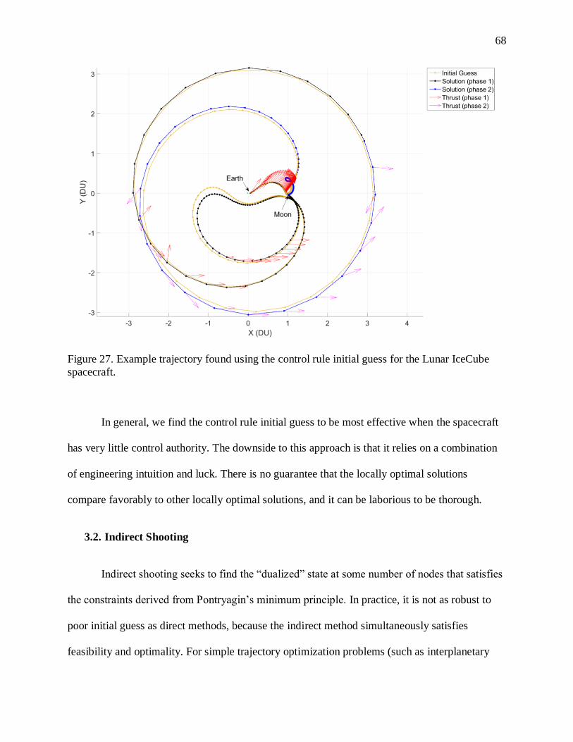
68

Figure 27. Example trajectory found using the control rule initial guess for the Lunar IceCube

spacecraft.

In general, we find the control rule initial guess to be most effective when the spacecraft

has very little control authority. The downside to this approach is that it relies on a combination

of engineering intuition and luck. There is no guarantee that the locally optimal solutions

compare favorably to other locally optimal solutions, and it can be laborious to be thorough.

3.2. Indirect Shooting

Indirect shooting seeks to find the “dualized” state at some number of nodes that satisfies

the constraints derived from Pontryagin’s minimum principle. In practice, it is not as robust to

poor initial guess as direct methods, because the indirect method simultaneously satisfies

feasibility and optimality. For simple trajectory optimization problems (such as interplanetary

69

transfers), indirect shooting can be robust to poor initial guess. For difficult problems (such as

transfers between three-body orbits), we find it effective to initialize indirect shooting with a

solution found with the direct method. Indirect shooting has an advantage over direct shooting in

that it can find solutions that more accurately satisfy the necessary conditions for optimality.

For indirect methods (either single shooting or multiple shooting), it is critical to use

homotopy to start with a smooth control law, then transition to the minimum fuel solution. This

chapter began by comparing 3 homotopic approaches, identifying the minimum-energy and

sigmoid-smoothed objective functions as the most helpful for our problems. Homotopy is used to

find the minimum fuel solution from the smooth solution.

The previous section described two methods for finding the minimum-energy solution

with direct multiple shooting. It is straightforward then to initialize indirect shooting with the

minimum-energy objective function. As discussed in the previous section, three-body transfers

can have many topologically-distinct locally optimal solutions. We find that the optimal

trajectory for the minimum-energy objective is often quite close to the optimal trajectory for the

minimum-fuel objective. Thus, the minimum-energy solution is a good initial guess for the

minimum-fuel (or sigmoid-smoothed minimum-fuel) objective. Figure 28 shows an example

transfer from a DRO to an NRHO, with both the minimum energy and minimum fuel solutions.

Thrust is scaled differently for the two trajectories for visualization only.

70

Figure 28. Comparison of minimum energy and minimum fuel trajectories for DRO-to-NRHO

transfer.

The control profile for the same transfer is shown in Figure 29. The direct method

changes control only at nodes; thus, there is a time delay between the direct minimum energy

control and the indirect minimum energy control. It is clear that the direct method gives a good

initial guess for the indirect method. It is also clear that, in this case, the sigmoid-smoothed

minimum fuel solution is very close to the minimum energy solution. Homotopy is a successful

method to convert the smoothed minimum fuel solution to the minimum fuel solution.

71

Figure 29. Comparison of control profiles for minimum energy and smoothed minimum fuel

objectives.

At every node, the state and costate are defined as optimization variables. The “dualized”

state is constructed from its parts.

𝑿𝑖 = [𝒓𝑖𝑇 , 𝒗𝑖

𝑇 , 𝝀𝑟,𝑖𝑇 , 𝝀𝑣,𝑖

𝑇 ]𝑇 (71)

The objective with the indirect multiple shooting step is to simultaneously enforce the dynamics

for the states and costates. The dualized state 𝑿𝑖 is propagated to time 𝑡𝑖+1, giving us 𝑿𝑖+1𝑝𝑟𝑜𝑝

.

Propagation uses the optimal control derived from Pontryagin’s minimum principle. The error in

dynamics is then

𝒉𝑖+1 = 𝑿𝑖+1 − 𝑿𝑖+1𝑝𝑟𝑜𝑝 . (72)

Using finite differences, the Jacobian of all the 𝒉𝑖 terms with respect to all the dualized states 𝑿𝑖

is computed. Ordinary least squares or the NLsolve package is then used iteratively to bring all

𝒉𝑖 below some small tolerance. For single shooting, we use the NLsolve package in Julia to find

72

the set of initial adjoints 𝝀(𝑡0) that lead to the target state 𝒙𝒇. NLsolve uses a trust region method

which converges more reliably than ordinary least squares. Automatic differentiation is used to

compute the Jacobian. For multiple shooting, we use ordinary least squares because the NLsolve

computational overhead grows quickly with the number of variables.

3.2.1. Homotopy

Homotopy, or continuation, consists of solving a series of similar problems, gradually

changing a parameter of interest which defines each solution. In this case, we begin with a

smooth, easily-differentiable control law, then iteratively arrive at the “bang-bang” fuel-optimal

solution. Homotopy is helpful for indirect methods because the fuel-optimal solution is highly

sensitive to the adjoints and has a narrow basin of attraction. Homotopy for optimal control has

been used by various results in the literature [29], [84]–[88]. Starting with a less sensitive control

law widens the basin of attraction and makes it easier to find a feasible solution. Once a feasible

solution is identified, it is simple to transform it into an optimal solution by defining a series of

optimal control problems, with the solution to one used as the initial guess for the next.

We compare three homotopy methods from the literature, which we refer to as 𝛼

homotopy, 𝑝 homotopy, and sigmoid homotopy. As described previously, the minimum fuel

solution comes from minimizing the integral of

𝐿 = |𝒖(𝑡)| (73)

over time. From Pontryagin’s principle, we find the following control law which minimizes the

propellant used:

𝒂𝑢 = {

𝟎3 𝑖𝑓 𝑆 < 0

−𝑢𝑚𝑎𝑥�̂�𝑣 𝑖𝑓 𝑆 > 0indeterminate 𝑖𝑓 𝑆 = 0

(74)

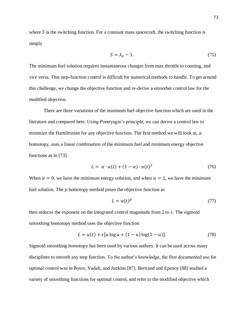
73

where 𝑆 is the switching function. For a constant mass spacecraft, the switching function is

simply

𝑆 = 𝜆𝑣 − 1. (75)

The minimum fuel solution requires instantaneous changes from max throttle to coasting, and

vice versa. This step-function control is difficult for numerical methods to handle. To get around

this challenge, we change the objective function and re-derive a smoother control law for the

modified objective.

There are three variations of the minimum fuel objective function which are used in the

literature and compared here. Using Pontryagin’s principle, we can derive a control law to

minimize the Hamiltonian for any objective function. The first method we will look at, 𝛼

homotopy, uses a linear combination of the minimum fuel and minimum energy objective

functions as in [73].

𝐿 = 𝛼 ∙ 𝑢(𝑡) + (1 − 𝛼) ∙ 𝑢(𝑡)2 (76)

When 𝛼 = 0, we have the minimum energy solution, and when 𝛼 = 1, we have the minimum

fuel solution. The 𝑝 homotopy method poses the objective function as

𝐿 = 𝑢(𝑡)𝑝 (77)

then reduces the exponent on the integrated control magnitude from 2 to 1. The sigmoid

smoothing homotopy method uses the objective function

𝐿 = 𝑢(𝑡) + 𝜖[𝑢 log 𝑢 + (1 − 𝑢) log(1 − 𝑢)]. (78)

Sigmoid smoothing homotopy has been used by various authors. It can be used across many

disciplines to smooth any step function. To the author’s knowledge, the first documented use for

optimal control was in Byers, Vadali, and Junkins [87]. Bertrand and Epenoy [88] studied a

variety of smoothing functions for optimal control, and refer to the modified objective which

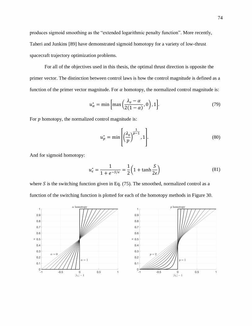
74

produces sigmoid smoothing as the “extended logarithmic penalty function”. More recently,

Taheri and Junkins [89] have demonstrated sigmoid homotopy for a variety of low-thrust

spacecraft trajectory optimization problems.

For all of the objectives used in this thesis, the optimal thrust direction is opposite the

primer vector. The distinction between control laws is how the control magnitude is defined as a

function of the primer vector magnitude. For 𝛼 homotopy, the normalized control magnitude is:

𝑢𝛼

∗ = min [max (𝜆𝑣 − 𝛼

2(1 − 𝛼), 0) , 1]. (79)

For 𝑝 homotopy, the normalized control magnitude is:

𝑢𝑝∗ = min [(

𝜆𝑣

𝑝)

1𝑝−1

, 1]. (80)

And for sigmoid homotopy:

𝑢𝜖

∗ =1

1 + 𝑒−𝑆/𝜖 =

1

2(1 + tanh

𝑆

2𝜖) (81)

where 𝑆 is the switching function given in Eq. (75). The smoothed, normalized control as a

function of the switching function is plotted for each of the homotopy methods in Figure 30.

75

Figure 30. Comparison of 3 control homotopy methods.

In principle, any of these homotopy methods should yield equivalent results. In practice,

we find that the sigmoid homotopy is much easier to converge on than the other methods. The 𝛼

homotopy method is discontinuous at the minimum and maximum control, 𝑝 homotopy is

smooth at the minimum control but discontinuous at the maximum control, and sigmoid

homotopy is always smooth. For numerical methods, it is important to have smooth,

differentiable functions. In this thesis, 𝑝 homotopy and sigmoid homotopy were both

implemented in single- and multiple-shooting algorithms. We find that for an equivalently sharp

bang-bang solution with two-body dynamics, it takes about 20 intermediate values of 𝑝 to

converge, while it only takes about 3 intermediate values of 𝜖 to converge. In other words, we

can take much larger steps in sigmoid homotopy than 𝑝 homotopy. For CRTBP dynamics, both

homotopy methods require a greater number of intermediate values to converge than for two-

body dynamics. The advantage of 𝑝 homotopy is that it is convenient to define the 𝑝 = 2

objective function for direct optimization, giving us an accurate estimate of the adjoints for

indirect optimization.

76

3.2.2. Initial Guesses for Indirect Method

3.2.2.1. Single Shooting

In this thesis, single shooting is only used for two-body dynamics. We always begin with

the sigmoid-smoothed minimum fuel objective function. Assuming the endpoints and time of

flight are feasible for the propulsion system, we can solve the TPBVP very easily with indirect

single shooting. The following algorithm was found to be highly effective and simple to

implement:

i. Initialize 𝝀0 as a random vector drawn from 𝒩(0,1).

ii. Try single shooting with sigmoid-smoothed control switching.

iii. If it converges, move on to homotopy (described in next sub-section).

iv. If it does not converge, try increasing the thrust limit by 1.5x, then reducing the thrust

limit back to the original value.

v. If it still has not converged, try a new random draw for 𝝀𝟎.

vi. Repeat until solution converges.

The strategy of artificially increasing and then decreasing the thrust limit helps the optimizer get

out of locally infeasible areas of the solution space. For the Earth-Venus rendezvous problem, we

find that 461 out of 1,000 random draws (46%) of 𝝀0 converge. Without using the trick of

increasing and decreasing thrust, we find that 112 out of 1,000 random draws (11%) of 𝝀0

converge.

For two-body problems, we define the target state and the error relative to the target state

with the modified equinoctial elements. Using orbital elements works better than Cartesian states

because there is a more linear relationship between 𝝀0 and 𝒙𝑓. Unfortunately, we do not have

any equivalent set of orbital elements that describe motion in three-body dynamics.

77

As an example, consider a low-thrust Earth to Venus rendezvous. The journey starts at

Earth with 𝑉∞ = 0 on 1-September-2022 and ends 600 days later at Venus with 𝑉∞ = 0. The

endpoints and time of flight are fixed. Mass is constant at 1000 kg. Thrust limit is constant at 0.4

N. An example progression of the iterations to convergence is plotted in Figure 31. The thick

black line represents the converged solution. Homotopy then reduces the control-smoothing

parameter. The fuel-optimal solution is shown in Figure 32.

Figure 31. Earth-to-Venus example, showing single shooting intermediate solutions.

78

Figure 32. Example fuel-optimal trajectory from Earth to Venus.

For two-body dynamics, even a poor initial guess can converge. There is no need for

prior steps. Each trial is fast (0.36 seconds for the Earth-Venus problem), so if one guess does

not converge, it is painless to try a new guess.

3.2.2.2. Multiple Shooting

The random guess strategy can be used for indirect multiple shooting, but only a small

percentage of random guesses will converge. It is more effective in most cases to begin with

direct multiple shooting, then use the direct solution to initialize the indirect method. If we have

a converged solution from direct multiple shooting, we can estimate the adjoints from the control

law. For instance, if we have the minimum energy solution from direct multiple shooting, then

we know it obeys the control law

𝒂𝑢 = −

1

2𝝀𝑣 (82)

or, equivalently,

79

𝝀𝑣 = −2𝒂𝑢. (83)

Note that this simple estimate does not consider the thrust limit. We can get the best estimate of

𝝀𝑣 when the thrust limit is not active. For two-body dynamics, 𝝀𝑟 is simply the rate of change of

𝝀𝑣. We can approximate 𝝀𝑟 at discrete times 𝑡𝑖 as

𝝀𝑟(𝑡𝑖) = −�̇�𝑣 ≈ −

𝝀𝑣(𝑡𝑖+1) − 𝝀𝑣(𝑡𝑖)

𝑡𝑖+1 − 𝑡𝑖. (84)

For three-body dynamics, the rate of change of 𝝀𝑣 is given by

𝝀�̇� = −𝝀𝑟 + [

2𝜆𝑣,𝑦

−2𝜆𝑣,𝑥

0

] (85)

which can then be solved for 𝝀𝑟.

𝝀𝑟 = −�̇�𝑣 + [

2𝜆𝑣,𝑦

−2𝜆𝑣,𝑥

0

] (86)

The �̇�𝑣 term is approximated as in Eqn. (82). We find that this approximation works well in

practice.

3.2.3. Example Transfers with Indirect Method

As an example, consider a low-thrust transfer from an L2 halo orbit to a near-rectilinear

halo orbit (NRHO). An NRHO is simply a specific member of the halo orbit families. Since the

orbits part of the same family, the trajectory stacking initial guess is appropriate here. The guess

does not have to be accurate – it simply needs to capture the general shape of the optimal

transfer. Direct multiple shooting struggled to converge completely on this transfer because the

end state is a close approach to the Moon. The nearly-converged solution from direct multiple

shooting is shown in Figure 33, with the control profile in Figure 34.

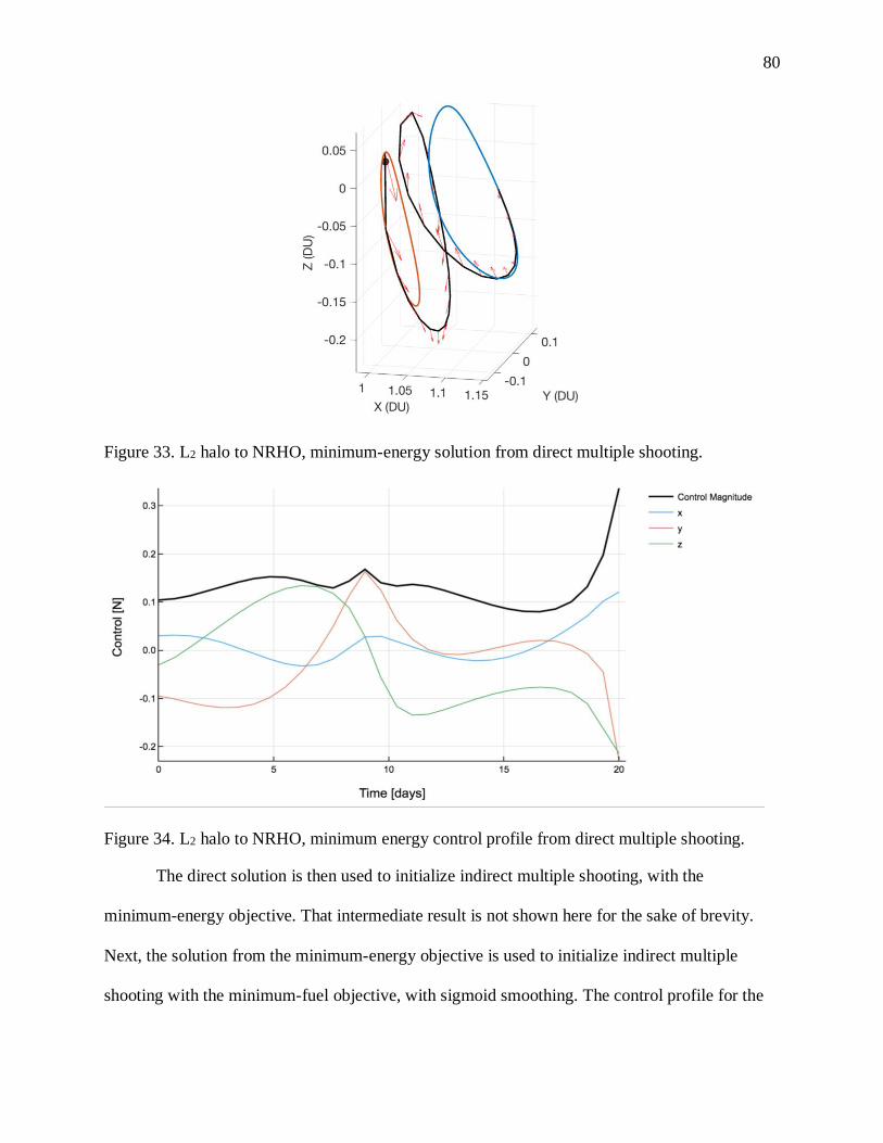
80

Figure 33. L2 halo to NRHO, minimum-energy solution from direct multiple shooting.

Figure 34. L2 halo to NRHO, minimum energy control profile from direct multiple shooting.

The direct solution is then used to initialize indirect multiple shooting, with the

minimum-energy objective. That intermediate result is not shown here for the sake of brevity.

Next, the solution from the minimum-energy objective is used to initialize indirect multiple

shooting with the minimum-fuel objective, with sigmoid smoothing. The control profile for the

81

smoothed minimum-fuel problem is shown in Figure 35. The control is only slightly different for

the minimum-energy and smoothed minimum-fuel cases. Next, homotopy is used to reduce the

smoothing parameter and arrive at the minimum fuel solution. Figure 36 shows the progression

of the control magnitude.

Figure 35. L2 halo to NRHO, smoothed minimum fuel control profile from indirect multiple

shooting.

Figure 36. L2 halo to NRHO, control law homotopy.

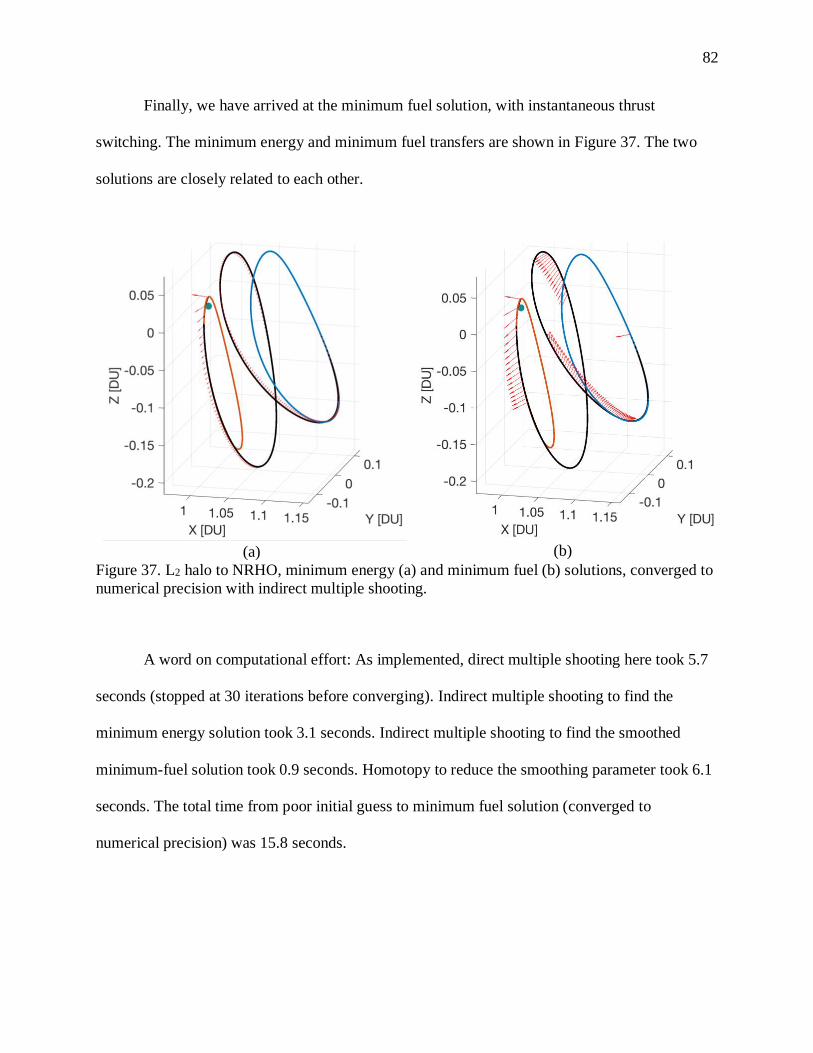
82

Finally, we have arrived at the minimum fuel solution, with instantaneous thrust

switching. The minimum energy and minimum fuel transfers are shown in Figure 37. The two

solutions are closely related to each other.

(a)

(b)

Figure 37. L2 halo to NRHO, minimum energy (a) and minimum fuel (b) solutions, converged to

numerical precision with indirect multiple shooting.

A word on computational effort: As implemented, direct multiple shooting here took 5.7

seconds (stopped at 30 iterations before converging). Indirect multiple shooting to find the

minimum energy solution took 3.1 seconds. Indirect multiple shooting to find the smoothed

minimum-fuel solution took 0.9 seconds. Homotopy to reduce the smoothing parameter took 6.1

seconds. The total time from poor initial guess to minimum fuel solution (converged to

numerical precision) was 15.8 seconds.

83

4. Families of Trajectories

Gradient-descent optimization schemes are only ever guaranteed to find local optima.

Except for simple problems which can be solved analytically, it is hard to determine how many

local optima there are. The simplest “optimization” problem in astrodynamics is Lambert’s

problem, which assumes a two-impulse solution. Even in such a simple case, there are at least

two solutions: one prograde and one retrograde. For most problems of this sort, it is easy to

choose the direction of motion which has a drastically lower cost. Even in two-body dynamics,

transfers with longer times of flight have several local optima, and the most practical way to

choose the best one may be to evaluate them all. In three-body dynamics, it is harder to predict

the number and location of local optima.

In this chapter, we explore transfers between DROs, between halo orbits, and from DRO

to halo orbit. Some families of optimal continuous-thrust transfers are studied, where each family

represents a set of optimal trajectories with fixed endpoints and varying time of flight. In all

cases, the minimum-energy objective is used, with unconstrained thrust. Spacecraft mass is 1,000

kg. Although many of the transfers shown are impractical, understanding the extent of each

family gives us insight into the local optima that optimization algorithms get drawn into.

To develop the families, first the methods from Chapter 3 are used to find a nominal

transfer. Then, continuation is used to gradually either increase or decrease the time of flight. At

each step, the previous converged solution is used as the initial guess. Each solution is solved

with indirect multiple shooting to a normalized constraint tolerance of 10-10. Each family is

continued as far as possible in time of flight. Additional solutions may exist for each family

beyond the region shown, but they are highly sensitive.

84

4.1. DRO to DRO

This first example is perhaps the simplest three-body orbit transfer: from one DRO to

another. The transfer is simple compared to other three-body transfers because both endpoints

are stable and closely resemble two-body orbits about the Moon. Intuition from two-body

dynamics can give a “close” initial guess of the shape of optimal transfers. Three families of

transfers are studied: 1-revolution, 2-revolutions, and 3-revolutions. A “revolution” here is

comparable to completing one period of a DRO.

For all three families, the same endpoints are used. These are given in Table 3. These

states were chosen as a 3𝜋/2 (retrograde) revolution from the +x axis crossing. Mass is chosen to

be constant at 1,000 kg, so that the thrust magnitude values are relatable to current EP systems.

Table 3. Initial and final states for DRO-to-DRO families.

Initial state Final state

𝑥 [DU] 0.9833680935501955 0.9888400743204971

𝑦 [DU] -0.2592089673653552 -0.0945408587696672

𝑧 [DU] 0 0

�̇� [DU/TU] -0.3513412950335397 -0.4286151099601722

�̇� [DU/TU] -0.008333463797646103 -0.0030943213818694906

�̇� [DU/TU] 0 0

Jacobi integral [-] 2.924986538267906 3.0250509792248423

The optimal transfer in this case is simply a spiral from one DRO to the other. We show these

high-cost solutions to such a simple transfer as a motivational example; the optimal solution is

not always so intuitive.

The 1-revolution family is plotted in Figure 38, the 2-revolution family in Figure 39, and

the 3-revolution family in Figure 40. The transfers plotted are separated in time of flight by 1 day

85

each. Families 2-3 were extended as far as possible, while Family 1 was stopped manually at 125

days.

Figure 38. Minimum energy DRO-to-DRO, family 1.


86


Families 1-2 develop interesting “loop-de-loops” in the vicinity of the Earth-Moon L3

libration point. Family 3 seems to end before the increase in time of flight leads to these kinds of

features. Family 3 could not be extended further, even with continuation step size reduced from

0.5 days down to 10-5 days. Further improvements to the formulation of the optimization

problem could extend this family to higher times of flight if the family continues to exist.

Optimal transfers, such as these, are 12-dimensional Hamiltonian systems, and the

Hamiltonian can be computed as in Eq. (16). For a single transfer, the Hamiltonian is constant

throughout. The families of solutions can be directly compared to each other by plotting the

Hamiltonian value as a function of time of flight, as in Figure 41.

87

Figure 41. DRO-to-DRO, Hamiltonian value for each family as a function of time of flight.

It is clear that the “most optimal” solution family varies as a function of time of flight. At some

times, two families have exactly the same Hamiltonian. Another way we can compare the

families is with the maximum control magnitude required. Remember that the control magnitude

is unconstrained and is instead determined by the minimum-energy objective function. Typically

for these transfers, the maximum control magnitude is only necessary for a short duration, and

adjusting the endpoints could reduce it.

Figure 42 shows the maximum control magnitude required for each family. We see that

the control authority required to fly each family of transfers varies as a function of time. Again,

the “best” family to fly depends on the time of flight. Although most of the transfers shown here

are unnecessarily high-cost, they are used here to illustrate the diversity of the set of optimal

solutions.

88

Figure 42. DRO-to-DRO, maximum control magnitude for each family as a function of time of

flight.

4.2. L2 Halo to L2 Halo

This example is very similar to the DRO-to-DRO transfers in the previous section. 1-, 2-,

and 3-revolution transfers are used to initialize families of solutions, and each family is

continued to the minimum and maximum time of flight where the optimization algorithm can

converge. For this transfer, there is also a fourth family identified, which departs the moon

entirely, spending up to several months in the vicinity of the L3 libration point before returning to

the L2 halo orbit. A “revolution” here is analogous to completing one period of a halo orbit. For

all four families, the same endpoints are used. These are given in Table 4, chosen as the +x axis

crossing. Mass is chosen to be constant at 1,000 kg, so that the thrust magnitude values are

relatable to current electric propulsion systems.

89

Table 4. Initial and final states for L2-to-L2 families.


𝑥 [DU] 1.017622294477337 1.043509065132913

𝑦 [DU] 0 0

𝑧 [DU] -0.06992934709718 -0.07558521319065699

�̇� [DU/TU] 0 0

�̇� [DU/TU] 0.48658120798033794 0.39312872806256893

�̇� [DU/TU] 0 0

Jacobi integral [-] 3.0327000279575405 3.060000021454574

As with the DRO-to-DRO case, the optimal transfer is easy to intuit. The L2 halo orbits

are themselves members of a family of ballistic, periodic solutions to the CR3BP. It is simple to

follow a “corkscrew” motion to transfer from one halo orbit to the other. Again, we show these

high-cost solutions to such a simple transfer as a motivational example; the optimal solution is

not always so intuitive.

The 1-revolution family is plotted in Figure 43, the 2-revolution family in Figure 44, and

the 3-revolution family in Figure 45. A fourth family of transfers also exists and is shown for this

problem in Figure 46. Each of the transfers plotted are separated in time of flight by 1 day each.

As a reminder, the figures are in the dimensionless, rotating reference frame, with Earth

stationary at [−𝜇, 0, 0] and Moon at [1 − 𝜇, 0, 0].

90

Figure 43. Minimum energy L2-to-L2, family 1.


91



92

These four families of transfers can be directly compared by plotting the Hamiltonian

value for each of the families as a function of time of flight. The Hamiltonian is shown in Figure

47, with a zoomed-in view in Figure 48. The maximum thrust magnitude is shown in Figure 49.

Figure 47. L2-to-L2 halo, Hamiltonian value for each family, as a function of time of flight.

Figure 48. L2-to-L2 halo, Hamiltonian value for each family, as a function of time of flight,

zoomed-in view.

93

Figure 49. L2-to-L2 halo, maximum control magnitude for each family, as a function of time of

flight.

Once again, we find that the “most optimal” family varies depending on the time of

flight. For some transfer durations, there are multiple families to choose from. It is not always

clear which family to choose. In cases where two or more families intersect, the optimizer could

easily get confused and struggle to converge. Families 1, 2, and 3 each have a very low-cost

member (at the trough of each family in Figure 49) that is a minimum of the total control effort.

If the maximum control available for a mission were even lower than 0.025 N, similar families

could be found with increasing numbers of revolutions. Since the initial and final halo orbits

have different Jacobi integrals, there is no “free” heteroclinic transfer available.

94

4.3. DRO to L2 Halo

For the DRO to L2 halo orbit case, we examine four individual members of overlapping

families. The same initial state, final state, and time of flight are used for each of the four

transfers shown in Figure 50. Time of flight is 30 days. The initial and final states are given in

Table 5. Mass is chosen to be constant at 1,000 kg, so that the thrust magnitude values are

relatable to current electric propulsion systems. The transfers shown were generated by randomly

guessing the states and controls several times. Direct multiple shooting was used first because of

its robustness to poor initial guess. Then, indirect multiple shooting was used to reduce the

constraint defects.

Transfer #1

Transfer #2

95

Transfer #3

Transfer #4

Figure 50. Unique local solutions for minimum energy DRO-to-L2 halo.

Table 5. Initial and final states for DRO-to-L2 families.


𝑥 [DU] 0.9833680935501955 1.1423846031874245

𝑦 [DU] -0.2592089673653552 0

𝑧 [DU] 0 0.15970542125529671

�̇� [DU/TU] -0.3513412950335397 0

�̇� [DU/TU] -0.008333463797646103 -0.2224918026509407

�̇� [DU/TU] 0 0

Jacobi integral [-] 2.924986538267906 3.060000007205874

These unique solutions can be classified by their Hamiltonian values and maximum

control magnitudes, provided in Table 6.

96

Table 6. Key descriptors of the unique DRO-to-L2 halo transfers found.

Transfer # Hamiltonian [-] Max control magnitude [N]

1 -3.9180x10-4 0.341

2 -3.4330x10-3 0.683

3 4.3331x10-3 0.780

4 -1.0441 3.614

The required control magnitude can generally be reduced for each family by adjusting the

endpoints. For example, adding a ballistic segment to the beginning of the transfer and re-solving

can help the optimization algorithm spread a large initial maneuver over a longer time of flight.

The existence of these local optima makes the initial guess very important. When a good

initial guess is available, it helps the optimization algorithm choose the correct local optimum.

When there is no initial guess available, the random guess method introduced in Chapter 3 is an

effective way to explore the available options.

97

5. Neural Networks Applied to Optimal Control

In this chapter, we introduce neural networks as a practical tool for astrodynamics. Many

engineering disciplines make use of linear approximations to solve a wide array of problems.

Some relationships cannot be reasonably approximated as linear; in those cases, one approach is

to use a higher-order polynomial basis function for the approximation. Polynomial chaos (PC) is

a powerful tool to build nonlinear relationships between any set of inputs and outputs, with

orthogonal polynomial basis functions used to approximate the relationship. References [90]–

[92] introduced PC to astrodynamics and found that it has much higher accuracy than linear

approximations, while being much faster to evaluate than the true dynamics (in that case, a

Monte Carlo analysis). We begin this chapter by comparing neural networks (NNs) to PC and

find that, just as PC extends the range and accuracy of linear assumptions, NNs extend the range

and accuracy of PC. Both PC and NNs are ways to construct approximate models of nonlinear

systems. We find that PC is a better choice for simple problems, but NNs are more robust. NNs

work well beyond the practical range of systems that can be modeled by PC.

With this justification of NNs in hand, we then apply the technique to a new problem that

previous methods have not been able to consider: optimal low-thrust trajectory correction. We

demonstrate that the control profile of a perturbed trajectory can be near-instantly corrected by

evaluating a neural network. This is done by generating hundreds of sample trajectories in the

vicinity of the nominal trajectory, then training a neural network to map the perturbed state to the

perturbed adjoints. Some potential applications are discussed, including: missed thrust analyses

during mission planning, Monte Carlo analyses during maneuver planning, and spacecraft

onboard navigation.

98

5.1. Uncertainty Propagation

5.1.1. Polynomial Chaos

To provide some motivation for using neural networks to model astrodynamics systems,

we will first examine another method: polynomial chaos (PC). Although mathematically distinct,

polynomial chaos expansions (PCEs) and NNs are conceptually similar. In PC, a polynomial

mapping is created to approximately map the uncertainty in a set of input variables to the

uncertainty in a set of output variables. A small number (typically on the order of hundreds) of

training samples are used to create the mapping (the polynomial chaos expansion). “Training”

the PCE consists of solving a system of linear equations and is thus very fast. The PCE can then

be sampled simply with matrix multiplication operations to approximate a large and

computationally expensive Monte Carlo analysis [93].

Jones, Doostan, and Born found that Generalized Polynomial Chaos can be applied to

orbital state uncertainty propagation [94]. As implemented there, Polynomial Chaos is essentially

a substitute for a Monte Carlo analysis. The result is a speedup of a few orders of magnitude, for

some small loss in accuracy. PCE has been used on the Magnetosphere Multi Scale (MMS)

mission to safely allow close formation flight. The MMS mission consists of four spacecraft

which make magnetic field measurements at each orbit apogee. When the measurements are

made, the spacecraft must be in a tetrahedron configuration. As a result of the science-driven

formation flight, the spacecraft are constantly at risk of colliding with each other. The

requirements on spacecraft safety are tight, so the common assumptions (Gaussian uncertainty

distribution and linear dynamics relative to the reference) are not accurate enough. Every orbit, a

Monte Carlo analysis is run to find the probability of collision, given the state estimate of each

spacecraft and their corresponding uncertainties. It would normally be impractical to run these

99

Monte Carlo analyses quickly enough to be useful for operations, but PC allows an equivalent

analysis to be run in a matter of minutes [92]. PC enables mission operations that would be

impractical otherwise, and NNs could extend that even further.

5.1.2. Comparison of Polynomial Chaos and Neural Networks

We will introduce the effectiveness of neural networks by comparing them to Polynomial

Chaos for spacecraft nonlinear uncertainty propagation. As discussed above, PC has been well

proven on this problem. The problem may be stated as: given an initial state 𝒙0 at time 𝑡0 and

corresponding initial covariance matrix, find the probability distribution of the state 𝒙𝑓 at a

future time 𝑡𝑓. For these methods, the state 𝒙(𝑡) may be propagated through any nonlinear

dynamics. Here, the dynamics are a two-body orbit. The initial state is a GEO-transfer orbit

(GTO) with the following orbital elements:

Table 7. Initial orbital elements for comparison of Polynomial Chaos and Neural Networks.

rp ra INC RAAN AOP TA

6678 km 42,200

km

20 deg 0 deg 0 deg 0 deg

The initial covariance matrix is diagonal, with uncertainty in position 𝜎𝑟 of 10 km and in velocity

𝜎𝑣 of 5 m/s.

Training samples are generated by sampling the initial uncertainty, then propagating each

sample forward to the final time 𝑡𝑓. Since we use two-body dynamics for this demonstration, the

samples are propagated analytically in a fraction of a second. However, these methods are

equally valid when samples are propagated with high-fidelity dynamics. The input to either PC

100

or the NN is the difference in state from the nominal initial condition. The output is the

difference in state from the nominal final condition.

𝐼𝑛𝑝𝑢𝑡 = 𝛿𝒙0 = 𝒙𝑠𝑎𝑚𝑝𝑙𝑒(𝑡0) − 𝒙𝑡𝑟𝑢𝑒(𝑡0) (87)

𝑂𝑢𝑡𝑝𝑢𝑡 = 𝛿𝒙𝑓 = 𝒙𝑠𝑎𝑚𝑝𝑙𝑒(𝑡𝑓) − 𝒙𝑡𝑟𝑢𝑒(𝑡𝑓) (88)

The same set of training samples are used to train both the polynomial chaos expansion and the

neural network. The polynomial chaos expansion is trained deterministically in under 1 second.

The neural network requires optimizing a set of a few tens of parameters, which in this case takes

a few tens of seconds (on a 2-core CPU).

The minimum number of training samples for PC depends on the number of random

inputs 𝑛 and the highest degree of the polynomials 𝑝.

𝑁𝑡𝑟𝑎𝑖𝑛 =

(𝑝 + 𝑛)!

𝑝! 𝑛!

(89)

For orbit state uncertainty propagation, 𝑛 is 6, and 𝑝 is a parameter we can choose to our liking.

Through trial and error, we found that 𝑝 = 4 works well for most problems, meaning that we

need at least 𝑁𝑡𝑟𝑎𝑖𝑛 = 210 training samples. We found that using two times the minimum

number generally works well.

There is no analytical way to define the number of training samples needed for NNs, but

NN performance improves monotonically with the number of training samples. The neural

network is trained and evaluated using the Neural Network Toolbox in MATLAB R2018a. We

use a feedforward neural network with three fully-connected hidden layers with 10 neurons each.

At training time, the test data is divided randomly into 70% for training, 15% for validation, and

15% for test. The Levenberg-Marquardt optimization method is used for training, with the

objective of minimizing the mean squared error (MSE). The NN was given 1,000 epochs

(iterations) to train.

101

The following examples map uncertainty from initial time 𝑡0 to a fixed final time 𝑡𝑓.

RMS error is compared between polynomial chaos and neural network (relative to the “truth”,

where each initial state is propagated through the true nonlinear dynamics). We see that for short

propagation times, polynomial chaos is up to 5 orders of magnitude more accurate than the

neural network. The NN error is acceptable for many applications, but the model is not able to

achieve better than 0.1 km position error and 0.03 m/s velocity error. As the propagation time

grows, both methods are challenged, but the polynomial chaos model diverges sooner from the

truth. We use PC with order 𝑝 = 4 (420 samples) and with 𝑝 = 5 (1848 samples). The NN size is

constant throughout.

Table 8. PC and NN model errors with tf = 5 hours (1/2 orbit, near apogee).

PC

(420 samples)

NN

(420 samples)

PC

(1848 samples)

NN

(1848 samples)

RMS position error (km) 2.1E-4 3.0E-1 1.5E-6 1.6E-1

RMS velocity error (m/s) 8.8E-5 3.7E-2 3.4E-7 3.2E-2

Table 9. PC and NN model errors with tf = 10.5 hours (1 orbit, near perigee).

PC

(420 samples)

NN

(420 samples)

PC

(1848 samples)

NN

(1848 samples)

RMS position error (km) 5.9E2 1.1E1 5.5E2 1.4E0

RMS velocity error (m/s) 1.4E3 3.0E0 1.8E3 5.2E-1

Table 10. PC and NN model errors with tf = 21 hours (2 orbits, near perigee).

PC

(420 samples)

NN

(420 samples)

PC

(1848 samples)

NN

(1848 samples)

RMS position error (km) 3.2E3 3.3E1 4.4E3 2.9E0

RMS velocity error (m/s) 5.0E3 1.0E1 8.4E3 1.3E0

102

It was found that mapping uncertainty to the perigee of an eccentric orbit is a stressing

case for polynomial chaos. We see that using a higher order polynomial base (with

correspondingly more samples) does not help PC in that case, but the greater number of samples

does reduce the NN error by about one order of magnitude.

As a visual example, the initial uncertainty was sampled 10,000 times, then propagated

10.5 hours (about one complete orbit). The black dots are the results from a traditional Monte

Carlo run and are the “truth” reference. The polynomial chaos model breaks down, especially

near perigee, while the neural network still matches most of the truth samples very closely.

Figure 51 shows how the polynomial chaos model breaks down, while the neural network does

not. Earth is shown to scale.

Figure 51. Comparison of NN and PC for orbit uncertainty propagation.

With this simple demonstration, we can see that neural networks are a promising

technology to propagate uncertainty through time. Neural networks can be used similarly to

polynomial chaos, with some advantages and disadvantages. In the following section, we will

103

show how neural networks can map a different set of inputs and outputs to provide an optimal

correction to low-thrust trajectories.

5.2. Optimal Low Thrust Trajectory Correction

We now use neural networks (NNs) to “learn” an optimal control policy in the

neighborhood of a nominal optimal trajectory. Whereas previously we compared PCEs and NNs

to map 𝛿𝒙0 → 𝛿𝒙𝑓 (initial state variation, to final state variation), we now use NNs to map the

initial state variation 𝛿𝒙0 to initial adjoint variation 𝛿𝝀0 or to adjoint variation over time 𝛿𝝀(𝑡).

This lets us describe the optimal trajectories in a neighborhood near a nominal, optimal

trajectory. In this section, we develop the algorithm to build this empirical relationship, then

apply it to test cases in two-body and three-body dynamics.

5.2.1. Algorithm Description

The classical two-point boundary value problem (TPBVP) is the foundation of this work.

The problem is defined as: find the path that connects initial state 𝒙0∗ and final state 𝒙𝑓

∗, in time of

flight 𝑡𝑓, that minimizes the objective function 𝐽. Using Pontryagin’s minimum principle as

described in Section 2.2, we can define an optimal trajectory with a different set of parameters:

initial state 𝒙0, initial adjoint 𝝀0, and time of flight. If we choose 𝝀0 = 𝝀0∗ , then propagating the

dualized state through the dynamical system will define an optimal path which arrives at the final

state 𝒙𝑓∗. As a shorthand notation, the TPBVP {𝒙0

∗ , 𝒙𝑓∗ , 𝑡𝑓} has the solution {𝒙0

∗ , 𝝀0∗ , 𝑡𝑓}. This

definition of the TPBVP is sketched in Figure 52.

104

Figure 52. Conceptual drawing of TPBVP solved with indirect method.

If the initial state is perturbed by some small amount 𝛿𝒙0, we know intuitively that there

should exist some new initial adjoint 𝝀0 = 𝝀0∗ + 𝛿𝝀0 such that 𝒙(𝑡𝑓) = 𝒙𝑓

∗. In our shorthand

notation, the new problem {𝒙0∗ + 𝛿𝒙0, 𝒙𝑓

∗ , 𝑡𝑓} has the solution {𝒙0∗ + 𝛿𝒙0, 𝝀0

∗ + 𝛿𝝀0, 𝑡𝑓}. In

fact, when we use the solution {𝒙0∗ , 𝝀0

∗ , 𝑡𝑓} as an initial guess to the perturbed problem, the

optimization algorithms described in Chapter 3 can often converge in just one or two iterations.

As 𝛿𝒙0 grows larger, the nominal solution becomes a worse initial guess for the perturbed

problem.

There exists a (highly nonlinear) relationship between any of the parameters defining

problem {𝒙0, 𝒙𝑓, 𝑡𝑓} and the initial adjoints 𝝀0. This relationship is complicated and difficult to

model accurately with conventional methods. Neural networks are a modern tool that, as

discussed in Section 5.1.2, can be used to build empirical models between any related inputs and

outputs. A simple example would be to use NNs to build an approximate model between 𝛿𝒙0

and 𝛿𝝀0. Once this model is built, it would possible to use the model to generate new solutions

105

for perturbed initial conditions. The inputs and outputs of this simple example can be stated more

explicitly as:

𝐼𝑛𝑝𝑢𝑡 = 𝛿𝒙0𝑗

= 𝒙0𝑗 (𝑡0) − 𝒙∗(𝑡0), 𝑗 ∈ ℤ: 1 ≤ 𝑗 ≤ 𝑁𝑠𝑎𝑚𝑝𝑙𝑒𝑠 (90)

𝑂𝑢𝑡𝑝𝑢𝑡 = 𝛿𝝀0𝑗

= 𝝀0𝑗 (𝑡0) − 𝝀∗(𝑡0), 𝑗 ∈ ℤ: 1 ≤ 𝑗 ≤ 𝑁𝑠𝑎𝑚𝑝𝑙𝑒𝑠 . (91)

In Section 3.2, we discuss how single shooting is not appropriate for some problems because of

the extreme sensitivity between the initial adjoints and the final state. For the same reason, it is

difficult to map 𝛿𝒙0 → 𝛿𝝀0 accurately enough to come close to the target state 𝒙𝑓∗ .

A more accurate model can be built by mapping (𝛿𝒙0, 𝑡) → (𝛿𝝀(𝑡)). This is conceptually

similar to how multiple shooting is more robust than single shooting because variables are

specified throughout the transfer instead of just at the endpoints. Each NN input/output pair is

then given by:

[𝐼𝑛𝑝𝑢𝑡]𝑖

𝑗= [𝛿𝒙0

𝑗

𝑡𝑖

] , 𝑗 ∈ ℤ: 1 ≤ 𝑗 ≤ 𝑁𝑡𝑟𝑎𝑖𝑛 , 𝑖 ∈ ℤ: 1 ≤ 𝑖 ≤ 𝑚 (92)

[𝑂𝑢𝑡𝑝𝑢𝑡]𝑖𝑗

= [𝛿𝝀𝑣𝑗 (𝑡𝑖)] , 𝑗 ∈ ℤ: 1 ≤ 𝑗 ≤ 𝑁𝑡𝑟𝑎𝑖𝑛 , 𝑖 ∈ ℤ: 1 ≤ 𝑖 ≤ 𝑚 (93)

where 𝑁𝑡𝑟𝑎𝑖𝑛 is the number of sample trajectories generated, and 𝑚 is the number of times saved

per sample. The times 𝑡𝑖 are linearly spaced from 𝑡0 to 𝑡𝑓. The total number of input/output pairs

is 𝑁𝑡𝑟𝑎𝑖𝑛 × 𝑚. In this thesis, we found that 𝑁𝑡𝑟𝑎𝑖𝑛 = 100-500, 𝑚 = 30-100 works well. As used

with MATLAB Neural Network Toolbox, the inputs are a matrix of size [7 × (𝑁𝑡𝑟𝑎𝑖𝑛 ∙ 𝑚)] and

the outputs are a matrix of size [3 × (𝑁𝑡𝑟𝑎𝑖𝑛 ∙ 𝑚)].

To generate training samples, we solve 𝑁𝑡𝑟𝑎𝑖𝑛 optimal control problems in a small

neighborhood of each other. Once one nominal solution has been found, optimizing the nearby

solutions is fast (ranging between 0.1-5 seconds each, depending on the problem). We use

indirect multiple shooting with sigmoid homotopy as described in Section 3.2.1.

106

We numerically integrate validation trajectories to test the validity of the NN

approximate correction. An advantage of mapping (𝛿𝒙0, 𝑡) → (𝛿𝝀𝑣(𝑡)) is that the adjoints do

not need to be propagated. Within the derivatives function for numerical integration, the nominal

adjoints 𝝀𝑣∗ (𝑡) are spline interpolated, and the NN is evaluated to find 𝛿𝝀𝑣(𝑡). The corrected

adjoints 𝝀𝑣(𝑡) are found as

𝝀𝑣(𝑡) = 𝝀𝑣∗ (𝑡) + 𝛿𝝀𝑣(𝑡). (94)

Then, the control law is evaluated to find 𝒖(𝝀𝑣(𝑡)), the optimal control at time 𝑡. The complete

algorithm implemented in this thesis to use NN’s for optimal trajectory correction is as follows:

Step 1. Find nominal solution:

a. Use direct multiple shooting to find minimum energy solution.

b. Use indirect multiple shooting to find minimum energy solution.

c. Use indirect multiple shooting to find minimum fuel solution, with sigmoid-smoothed

control law (𝜖 = 1).

d. Use homotopy to reduce smoothing parameter and find minimum fuel solution with

bang-coast-bang thrust structure (𝜖 = 10−4).

e. Save nominal solution {𝒙0∗ , 𝝀∗(𝑡), 𝑡𝑓} for reference in Steps 2-4.

Step 2. Generate training samples:

a. Choose distribution of training samples 𝑃(𝛿𝒙0) to be the same as the distribution that

validation samples will be pulled from.

b. Perturb initial state by 𝛿𝒙0𝑖 , pulled from 𝑃(𝛿𝒙0), for 𝑖 ∈ 𝑁𝑡𝑟𝑎𝑖𝑛.

c. Use indirect multiple shooting to find minimum fuel solution with bang-coast-bang

thrust structure.

107

i. If problem converges immediately with small 𝜖 smoothing term, accept

solution and move on.

ii. If problem does not converge, raise 𝜖 until it does converge. Then, reduce 𝜖

back to the bang-coast-bang value, with intermediate 𝜖 value(s) as necessary.

d. Save solutions 𝒙0𝑖 , 𝝀𝑖(𝑡) for 𝑖 ∈ 𝑁𝑡𝑟𝑎𝑖𝑛.

Step 3. Train neural network:

a. Scale and shift NN inputs and outputs to be in range [-1, 1]

b. Choose NN size and training algorithm.

b. Call NN training library of choice (here, MATLAB Neural Network Toolbox).

Step 4. Validate neural network:

a. Perturb initial state by 𝛿𝒙0𝑗, pulled from 𝑃(𝛿𝒙0), for 𝑗 ∈ 𝑁𝑣𝑎𝑙𝑖𝑑𝑎𝑡𝑒 .

b. Propagate initial state forward in time, with control law corrected by NN.

i. Interpolate nominal adjoints 𝝀∗(𝑡) at current time.

ii. Evaluate NN to find 𝛿𝝀(𝑡).

iii. Compute control 𝒖(𝑡) according to optimal control policy.

c. Check error.

Depending on the problem and the availability of an initial guess, Step 1 (a-b) may be

skipped.

5.2.2. Proposed Application: Onboard Navigation

When an electric propulsion spacecraft is thrusting, it is constantly injecting errors into

the state knowledge. Orbit determination (OD) errors are compounded with maneuver execution

108

errors. Traditionally, a regular cadence of ground contacts is required to update the spacecraft’s

state estimate and upload new thrusting instructions. Frequent ground contacts can be costly

[95], [96]. Technologies in development by NASA and others can perform autonomous onboard

OD [97]–[99] and limited onboard maneuver planning [100]. Assuming onboard OD is available,

neural networks could be used for onboard maneuver planning. The general architecture

proposed is as follows:

Step 1. Given an initial covariance matrix, build a neural net as described above that

maps (𝛿𝒙(𝑡0), 𝑡) → (𝛿𝝀(𝑡)).

Step 2. Upload neural net to the spacecraft.

Step 3. When the spacecraft clock reaches the predefined checkpoint, it determines the

current state 𝒙0 via onboard OD, then calls the appropriate NN to map

(𝛿𝒙(𝑡0), 𝑡) → (𝛿𝝀(𝑡)). The updated control law is used until the next

checkpoint is reached.

In principle, this approach could allow a spacecraft to use far fewer ground contacts than

a conventional mission. As described so far, there is only one checkpoint at which the NN is

evaluated. The same methodology can be used to create any number of checkpoints so that the

small error of the NN approximation does not propagate too far downstream. The algorithms

described above are summarized visually in Figure 53.

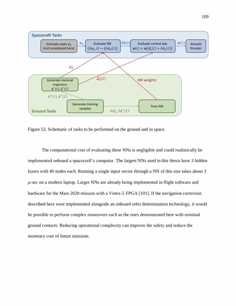
109

Figure 53. Schematic of tasks to be performed on the ground and in space.

The computational cost of evaluating these NNs is negligible and could realistically be

implemented onboard a spacecraft’s computer. The largest NNs used in this thesis have 3 hidden

layers with 40 nodes each. Running a single input vector through a NN of this size takes about 3

-sec on a modern laptop. Larger NNs are already being implemented in flight software and

hardware for the Mars 2020 mission with a Virtex-5 FPGA [101]. If the navigation correction

described here were implemented alongside an onboard orbit determination technology, it would

be possible to perform complex maneuvers such as the ones demonstrated here with minimal

ground contacts. Reducing operational complexity can improve the safety and reduce the

monetary cost of future missions.

110

5.2.3. Comparison to Results in Literature

Other researchers have independently begun to apply NNs to astrodynamics. To clarify

the contribution made in this thesis, we offer some direct comparisons here. The most closely-

related research to date comes from Izzo, Sprague, and Tailor [73], where a NN is used to map

state 𝒙(𝑡) to control 𝒖(𝑡) for a low-thrust rendezvous from Earth to Mars. A challenge identified

in [73] is that when mapping state directly to control, the thrust switching times are difficult to

capture accurately. In the present research, we choose to map state to adjoints, then compute the

control based on the optimal control policy. The adjoints follow a smooth trajectory, whereas the

controls are discontinuous. By mapping only continuous trajectories, we improve the accuracy of

the model. This thesis also improves on the accuracy in [73] by only mapping the trajectories

relative to a fixed reference trajectory. We feel that mapping absolute state to absolute control is

unnecessarily difficult; it is more useful to map state to control relative to a nominal path.

Izzo and various other co-authors have mapped state directly to control for other

aerospace dynamical problems, such as rocket landings and quadrotor paths [72], [73]. A variety

of authors dating back to 1948 [102] have considered artificial intelligence approaches to optimal

control. Other authors in the 1980s to 2000s have sought to apply neural networks to aircraft

flight control systems, offering greater modeling capability than traditional linear approximations

[103]–[106]. With these results and the contribution made by this thesis, it seems clear that NNs

have a place in aerospace guidance, navigation, and control.

5.2.1. Numerical Issues

To train an NN accurately enough to be useful for this problem, we need to have very

high-quality training samples. Solutions must be fully converged to near numerical precision, to

111

the point that the trajectory can be replicated nearly perfectly. If the solutions have not

completely converged, the NN will unsuccessfully try to “learn” numerical noise. When solving

nonlinear optimization problems, there are a number of ways that numerical issues can creep in

and reduce the accuracy of a solution. The three main numerical challenges encountered and

overcome in this research are: discontinuous thrust modeling, numerical integration accuracy,

and constraint convergence tolerance.

The primary tool to overcome the first two challenges is the sigmoid-smoothed control

law explained in Section 3.2.1. We use a smoothing parameter of 10-3 or 10-4, at which value the

control profile is imperceptibly different from a true “bang-coast-bang” structure. Even a small

smoothing parameter improves the numerical integration accuracy by preventing the ODE solver

from stepping over the control switching time. We use the “DifferentialEquations” package in

Julia to propagate with the Vern8 solver (a Runge-Kutta 8/7 method). Relative tolerance for

numerical integration is set to 10-13.

The accuracy of partial derivatives becomes important when tight convergence tolerance

is necessary. The convergence tolerance used for training samples was 10-10 (normalized units).

We find that using finite differenced derivatives are not effective to achieve this tolerance; with

finite differencing, the solution would indefinitely bounce around 10-8. Using dual numbers to

compute derivatives accurate to numerical precision made it easy to meet and exceed the 10-10

tolerance. Most training samples used in this thesis converged to about 10-12 or 10-13.

Indirect optimization is most natural for building the training samples in this thesis

because we use a NN to map states and adjoints. We recommend that future researchers using

NNs in any related way also use indirect optimization. While the indirect method is more

sensitive to the initial guess, it converges more quickly to tight tolerances when a good initial

112

guess is available. We found that the indirect method may reduce the constraint defects by up to

6 orders of magnitude in a single iteration.

5.2.2. Test Cases

The following test cases demonstrate the NN low-thrust trajectory correction algorithm

for realistic minimum-fuel orbit transfers in interplanetary (two-body) and Earth-Moon (three-

body) dynamics. The real test of accuracy is propagating a trajectory with the control law based

on the modified adjoints. The goal here is to simulate spacecraft operations. In these tests, we

“uplink” to the simulated spacecraft the same data as described in Figure 53.

5.2.2.1. Test Case 1 – Mars-to-Psyche Transfer

For our first test case of the neural network optimal control correction, we examine a

trajectory similar to the Psyche mission’s interplanetary transfer. Psyche’s transfer consists of an

Earth-Mars leg and a Mars-Psyche leg; here, we model only the Mars-Psyche leg. This test case

was chosen as a realistic scenario with two-body dynamics. It begins immediately after the Mars

flyby and ends with Psyche arrival. We use a constant spacecraft mass of 1,333 kg and a constant

thrust limit of 120 mN. The spacecraft departs Mars on 2023-05-23 and arrives at Psyche on

2026-03-14. The post-Mars-flyby condition is assumed to have 𝑉∞ of 3.3 km/s, in Mars’ velocity

direction.

The nominal solution was found by randomly guessing the initial adjoints 𝝀0, then using

single shooting to target the Psyche rendezvous. As described in Section 3.2, nearly half of all

random guesses converge for simple problems like this. The sigmoid control-smoothing

parameter 𝜖 is initially set to 1. When one of the random guesses of 𝝀0 converges, we then use

homotopy to reduce 𝜖 to 10-4, giving us the fuel-optimal solution. The nominal solution is plotted

in Figure 54, and the nominal control profile is shown in Figure 55.

113

Figure 54. Mars-to-Psyche nominal trajectory used in this analysis.

Figure 55. Mars-to-Psyche nominal control profile.

114

Once the nominal solution has been chosen, training samples are generated for the NN.

The initial covariance matrix is diagonal, with 1-𝜎 uncertainty in position of 20,000 km and in

velocity of 20 m/s (each axis). For this example, we use 𝑁𝑡𝑟𝑎𝑖𝑛 = 500 and 𝑚 = 50. The initial

covariance is randomly sampled 𝑁𝑡𝑟𝑎𝑖𝑛 times, and the perturbed initial conditions are re-

converged with single shooting. The total number of input/output pairs is 𝑁𝑡𝑟𝑎𝑖𝑛 × 𝑚 = 25,000.

Through trial and error, we found that a good size neural network for this problem is

[40, 40, 40] (3 hidden layers with 40 nodes each). Since part of what the NN learns is a time-

dependency, using multiple hidden layers converges more quickly than a single hidden layer

with the same total number of nodes. The choice to use multiple hidden layers was guided by the

intuition that recursive NNs (which can be unwrapped partially to become multi-layer

feedforward NNs) are good at modeling time-series data. Training was run overnight (10 hours)

on a 2-core laptop, and the final MSE of the NN was 3.0x10-7. Note that NN training is trivially

parallelizable and can take full advantage of many-core CPUs and GPUs when the hardware is

available.

After training, we validate the NN by propagating new random samples of the initial

distribution. If no correction is made to the control profile, the initial error grows large over time.

Histograms of the uncorrected final position and velocity error magnitudes are shown in Figure

56. When the NN correction is used, the final state error is reduced to be only slightly larger than

the numerical integration accuracy. Histograms of the corrected final position and velocity error

magnitudes are shown in Figure 57.

115

Figure 56. Mars-to-Psyche histograms of position and velocity errors, no correction.

Figure 57. Mars-to-Psyche histograms of position and velocity errors, with NN correction.

This example shows that it is possible to use an NN to accurately learn the optimal

correction 𝛿𝝀𝑣(𝑡) as a function of an initial perturbation 𝛿𝒙0, for two-body dynamics. In the

following examples, we use the CR3B dynamics, which are more challenging due to their

sensitivity.

5.2.2.2. Test Case 2 – CR3BP – DRO-to-NRHO

This test case uses two orbits that are of interest to the planned Deep Space Gateway: a

distant retrograde orbit (DRO) and a near-rectilinear halo orbit (NRHO). NRHO’s are part of the

116

L1 and L2 halo orbit families, and they are of interest for the planned Deep Space Gateway

because they are nearly stable [107]. Here, we chose a southern L2 NRHO (a spacecraft in this

orbit dwells mostly over the lunar south pole). The precise initial conditions of the initial orbit

and final orbit are given in Table 11 below.

Table 11. Initial and final conditions for DRO to NRHO transfer.


𝑥 [DU] 1.0773094647887356 0.9956461791199591

𝑦 [DU] 0 -0.04622742816025321

𝑧 [DU] 0 -0.05094004418576085

�̇� [DU/TU] 0 -0.08748056716039979

�̇� [DU/TU] -0.4697376289569243 0.11304919197855198

�̇� [DU/TU] 0 0.4906469979990478

Jacobi integral [-] 3.0250510239610913 3.0391699143345994

We use the methods described in Chapter 3 to develop a nominal trajectory. Spacecraft

mass is constant at 1,000 kg. Thrust limit is constant at 0.5 N. Direct multiple shooting was used

first with flexible endpoints and time of flight, to get a feel for what solutions should look like.

Once direct multiple shooting almost converged, the endpoints and time of flight were frozen to

get tight convergence on the minimum energy solution. The solution from direct multiple

shooting was then used to initialize indirect multiple shooting with the minimum energy

objective function. Time of flight was added at the NRHO arrival to reduce the thrust

requirement from the original solution. Once the thrust was acceptable (we arbitrarily used a

threshold of 0.5 N), we switched to the sigmoid-smoothed minimum fuel objective and used

homotopy to find the minimum fuel solution with a bang-coast-bang thrust profile. The nominal

trajectory is plotted in Figure 58, and the nominal control profile is plotted in Figure 59.

117

Figure 58. DRO-to-NRHO nominal trajectory.

Figure 59. DRO-to-NRHO nominal control profile.

118

Once a good nominal trajectory has been found, we can generate training samples for the

neural network. Since the CR3B dynamics are highly sensitive, we use a smaller perturbation

than for the interplanetary case. The initial covariance matrix is diagonal, with 1-𝜎 uncertainty in

position of 100 km and in velocity of 1 m/s. Davis et al. [107] find that realistic navigation errors

are about an order of magnitude smaller than this.

Using only 100 training trajectories did not work well for this problem – the MATLAB

NN Toolbox showed during training that the samples reserved for validation did not fit as

accurately as the samples used for training. Notice in Figure 60 that the Train subset of the

training data has nearly an order of magnitude lower mean squared error (MSE) than the

Validation subset of the training data. This is essentially over-fitting the data, and it is a sign that

the NN will not generalize well to new data.

Figure 60. MSE for the Train, Validation, and Test subsets of the training samples, with 100

sample trajectories.

119

There are two options to help the NN generalize better: reduce the size of the NN or add

more training samples. In this case, it was decided to add more samples. The NN size was held

fixed at [20, 20, 20] (3 fully-connected hidden layers with 20 nodes each). When the training

algorithm was run again with 500 training trajectories, it showed much better performance.

Figure 61 shows that with 500 training trajectories, the NN generalizes well (notice how the

Train, Validation, and Test performance are all close together). Training was run for 20 minutes

on a 2-core laptop, and the final MSE of the NN was 6.1x10-6.

Figure 61. MSE for the Train, Validation, and Test subsets of the training samples, with 500

sample trajectories.

It was found that for the problems modeled in this thesis, an appropriate neural network

size is three fully-connected hidden layers with 20-40 neurons each. Other researchers have

120

found that recurrent neural networks (RNNs) are effective at learning time-series relationships.

RNNs are often trained in an “unrolled” format, where they are equivalent to multi-layer

feedforward neural networks [66]. This intuition lead to using a multi-layer feedforward NN

rather than a single layer feedforward NN. Trial and error found that a three-layer NN was more

accurate than a single-layer NN with the same number of artificial neurons. To evaluate the

effectiveness of using fully-connected hidden layers, the set of all NN weights are plotted in

Figure 62.

Figure 62. Sorted magnitude of all NN weights.

None of the weights is close to numerical precision, with most being within a few orders of

magnitude of each other. Given this, we feel that using fully-connected layers is justified.

Once the NN has been trained, it can be used to generate control corrections for new

randomly perturbed initial states. We draw the new perturbed initial states from the same

121

distribution as the training data. We assume that the relative state estimate 𝛿𝒙0 is perfect. The

NN generates the time profile of the difference in adjoints 𝛿𝝀𝑣(𝑡) as a function of the initial state

relative to the nominal initial state. We then add the perturbed adjoints to the nominal adjoints,

yielding the NN’s approximation of the adjoints over time. We see in Figure 63 that the nominal

and corrected adjoints are very similar to each other.

Figure 63. DRO-to-NRHO nominal and corrected v over the trajectory, for 1 random sample.

Finally, we test the accuracy of the NN correction by propagating the entire transfer with

and without the correction. Figure 64 shows the uncorrected trajectories in red and the corrected

trajectories in green. Clearly, the NN correction keeps the transfer close to the nominal path,

while the uncorrected case quickly diverges and would require substantial maneuver re-planning.

Figure 65 -Figure 66 show the position and velocity errors, respectively, relative to the nominal

path.

122

Figure 64. DRO-to-NRHO trajectories with error.

Figure 65. DRO-to-NRHO position error.

123

Figure 66. DRO-to-NRHO velocity error.

From these figures, it is clear that the NN correction is able to reduce the error by over

two orders of magnitude. Recall that the NN correction targets the final state, not the nominal

path. If the NN correction were perfect, the error would drop to zero only at the final time. As-is,

the NN error at the final state is not zero, but it is smaller than the initial state error.

5.2.2.3. Test Case 3 – CR3BP – DRO-to-DRO

This test case considers a low-thrust transfer between two distant retrograde orbits

(DROs) in the Earth-Moon system. The initial states for the initial and final DRO’s are given in

Table 12. Such a transfer could be relevant to the Deep Space Gateway or other future missions.

Others have shown similar optimal transfers [108], [109]. Due to their stability and similarity to

two-body orbits, it is simpler to design a transfer between DROs than other three-body orbits.

The new contribution made by this thesis is the correction via neural network.

124

Table 12. Initial and final conditions for DRO to DRO transfer.


𝑥 [DU] 0.9833680935501955 0.9888400743204971

𝑦 [DU] -0.2592089673653552 -0.0945408587696672

𝑧 [DU] 0 0

�̇� [DU/TU] -0.3513412950335397 -0.4286151099601722

�̇� [DU/TU] -0.008333463797646103 -0.0030943213818694906

�̇� [DU/TU] 0 0

Jacobi integral [-] 2.924986538267906 3.0250509792248423

Once again, we use direct multiple shooting first to find the minimum-energy solution

with discretized control. Then, indirect multiple shooting is used to transition the minimum-

energy solution to the minimum fuel solution. Spacecraft mass is constant at 1,000 kg. The thrust

limit is constant at 0.15 N. The transfer time is exactly 20 days (including coasting periods found

by the optimizer at the start and end). The nominal trajectory is shown in Figure 67, and the

nominal control profile is shown in Figure 68. Transfer parameters used here are intended to be

realistic, but not based on any particular spacecraft.

125

Figure 67. DRO-to-DRO nominal trajectory.

Figure 68. DRO-to-DRO nominal control profile.

126

Here we use 𝑁𝑡𝑟𝑎𝑖𝑛 = 500 and 𝑚 = 50. Initial error in position is 100 km (1-𝜎, each

axis), and initial error in velocity is 1 m/s (1-𝜎, each axis).

The error over the duration of the transfer are shown in Figure 69 -Figure 70 for position

and velocity, respectively. The dotted line represents the mean error of 1,000 validation samples,

and the shaded areas represent the 98% confidence interval of error over time. Note that the

initial error for the corrected and uncorrected cases grow identically the same for the first few

days because of the initial coast period. As the thrust turns on, the NN correction reduces the

error. Remember that the goal is to reduce the error to zero only at the end time – not earlier in

the transfer.

Figure 69. DRO-to-DRO position error, with initial error 100 km, 1 m/s.

127

Figure 70. DRO-to-DRO velocity error, with initial error 100 km, 1 m/s.

Most of the thrusting takes place in the latter half of this transfer. As a result, the

corrected trajectories continue to drift apart from the nominal trajectory for the first 10 days.

From day 0 to day 10, the error grows by a factor of ~30x. Then, the control comes back on, and

the error is brought back down so that by the final time, the error relative to the nominal is

smaller than at the initial time. The error for the uncorrected case continues to grow dangerously.

This example illustrates the power of the NN approximation to accurately capture future control

updates as a function of error at an initial epoch.

5.2.2.4. Test Case 4 – CR3BP – L2 Halo-to-L2 Halo

The final test case is a low-thrust transfer from one L2 halo orbit to another, in the Earth-

Moon system. The initial conditions of the initial and final halo orbits are given in Table 13.

Table 13. Initial and final conditions for L2 to L2 transfer.


128

𝑥 [DU] 1.017622294477337 1.0621795348403944

𝑦 [DU] 0 0.1248245386078122

𝑧 [DU] -0.06992934709718 0.006374139014885798

�̇� [DU/TU] 0 0.08232796285860763

�̇� [DU/TU] 0.48658120798033794 0.10624585794520502

�̇� [DU/TU] 0 0.24400089457682106

Jacobi integral [-] 3.0327000279575405 3.060000021454574

Mass is constant at 1,000 kg, and thrust limit is constant at 0.1 N. The transfer time is 15 days. In

this case, ballistically propagating either orbit for any duration is a good initial guess for an

optimal transfer between them. A point on the initial halo orbit was picked arbitrarily to start the

transfer. Since this guess is close already, the direct method was not needed at all – we begin

with indirect multiple shooting for the smoothed fuel-optimal objective. Homotopy is then used

to sharpen the thrust switching. The nominal trajectory is shown in Figure 71, and the nominal

control profile is shown in Figure 72.

Figure 71. L2-to-L2 nominal trajectory.

129

Figure 72. L2-to-L2 nominal control profile.

For this example, we use 𝑁𝑡𝑟𝑎𝑖𝑛 = 500 and 𝑚 = 30. The NN size is [40, 40, 40] (3 fully-

connected hidden layers with 40 nodes each). Training time was about 4 hours on a 2-core

laptop. The results are plotted in the following figures. Figure 73 shows that without any

correction, the error in this case grows dramatically. The unstable dynamics are amplified by

following an incorrect control law. With the NN correction, there is still error, but it has been

greatly reduced to still consider the spacecraft to be “on” the halo orbit.

130

Figure 73. Low-thrust transfer from one L2 halo orbit to another, with error in the initial state.

Figure 74 shows the position error as a function of time, with and without the NN correction.

Figure 75 shows the velocity error. In each, the dotted line represents the mean error of 1,000

validation samples, and the shaded areas represent the 98% confidence interval of error over

time. Again, the error is maintained at the level of the initial state error.

131

Figure 74. L2-to-L2 position error over time.

Figure 75. L2-to-L2 velocity error over time.

132

6. Conclusion

6.1. Summary

This thesis deals with the problem of low-thrust trajectory optimization in the Earth-

Moon system. Several methods of optimal control are developed and shown to be effective.

Recognizing that trajectory optimization algorithms tend to spend an inordinate amount of time

stuck in the nonlinear programming (NLP) solver, we break down the sequential quadratic

programming (SQP) algorithm into its most basic parts. We simplify the optimal control problem

representation and show how even something as simple as a two-stage differential corrector can

be used to quickly generate optimal solutions in complex dynamics. The SQP algorithm is then

partially built back up, retaining the high performance and robustness to poor initial guess that

were demonstrated for the differential corrector approach. Using simplified NLP solution

methods revealed that endpoints and time of flight are the most difficult variables to converge

on, so quadratic terms were implemented selectively for the endpoint constraints.

This thesis shows that indirect multiple shooting with a smooth control law and automatic

differentiation are robust to poor initial guess, though not as robust as direct multiple shooting.

Given a reasonable initial guess, indirect multiple shooting is found to converge many times

faster than direct multiple shooting. Three common approaches to homotopy are compared, and

the sigmoid-smoothed control law is identified as the best for trajectory optimization.

In three-body dynamics, it is not always intuitive which of multiple local optima will be

the global best. While some of the approaches shown are robust to poor initial guess, we show

that various initial guesses should be used to explore multiple local optima.

133

The main novel contribution of this thesis is the application of artificial neural networks

(NNs) to astrodynamics. NNs are compared to polynomial chaos and found to generalize much

better than the orthogonal polynomial basis functions that polynomial chaos relies on. NNs are

then used to accurately correct a low-thrust trajectory relative to a reference trajectory, greatly

reducing the error in the achieved final state. This capability is envisaged for spacecraft onboard

navigation, as the approximate NN correction can be evaluated for a negligible computational

cost. A potential implementation for onboard trajectory correction is laid out.

This thesis contributes to a large body of knowledge accumulated over many decades

with regard to solving the optimal control problem. Some enhancements are presented that

improve the robustness and speed of solving trajectory optimization problems in the Earth-Moon

system. This thesis also forges new ground in the relatively new field of artificial intelligence,

applying cutting edge algorithms and tools to relevant technical challenges. The novel

developments described here advance NASA’s technology goals and contribute to the future of

crewed and robotic space missions in the Earth-Moon system.

6.2. Future Work

Neural networks have captured the interest of researchers for several decades, but it is

only recently that computer advancements have made them a practical reality. As NNs have

found widespread use with internet technology companies, the algorithms and software tools to

train and implement NNs have developed. We now can take advantage of the massive

investments in computer science to use this powerful tool for spacecraft optimal control. We see

a rich field of future work with NNs in astrodynamics and optimal control.

There are some specific next steps that are clear for the work presented in this thesis. One

is to sample the NN inputs more intelligently. In the present implementation, samples are from a

134

normal distribution. Other sampling schemes, such as Latin hypercube sampling, might capture

the same amount of information about the underlying dynamics with fewer total samples. The

benefit would be reduced sample generation time and NN training time.

In this thesis, the NN is used to compute a new path to the original target state. An

alternative formulation would be to compute the control to return to the nominal trajectory at

some fixed time in the future. For instance, the NN could guide the spacecraft to where it should

be, say, 5 days in the future.

It was found that there are often multiple local solutions for the same endpoints and time

of flight, and these local solutions come close to each other sometimes. In this thesis, NN

training was always performed within a single family of solutions. Future work could develop

the capability to “learn” multiple families of solutions. In some cases, it may be advantageous to

correct a trajectory onto a different family than the nominal transfer.

Other related potential applications of NNs in optimal control include (in two-body or

three-body dynamics): autonomous station-keeping (in which the thruster is off most of the

time), autonomous correction of man-revolution spiral trajectories (for instance, from a geo-

transfer orbit to a geostationary orbit), and autonomous rendezvous with low-thrust propulsion.

Although the NN inputs and outputs would need to be adjusted for these applications, the basic

methodology would be the same as shown in this thesis.

135

References

[1] K. Nishiyama, S. Hosoda, H. Koizumi, Y. Shimizu, I. Funaki, H. Kuninaka, M.

Bodendorfer, J. Kawaguchi and D. Nakata, “Hayabusa’s Way Back to Earth by

Microwave Discharge Ion Engines,” 46th AIAA/ASME/SAE/ASEE Joint Propulsion

Conference & Exhibit, AIAA 2010-6862, no. July, pp. 1–12, 2010.

[2] M. R. Drinkwater, R. Haagmans, D. Muzi, A. Popescu, R. Floberghagen, M. Kern and M.

Fehringer, “The GOCE gravity mission: ESA’s first core earth explorer,” in European

Space Agency, (Special Publication) ESA SP, 2006, vol. Frascati, no. SP-627, pp. 1–7.

[3] D. Doyle, G. Pilbratt and J. Tauber, “The Herschel and Planck Space Telescopes,”

Proceedings of the IEEE, vol. 97, no. 8, pp. 1403–1411, 2009.

[4] J. P. Gardner, J. C. Mather, M. Clampin, R. Doyon, M. A. Greenhouse, H. B. Hammel, J.

B. Hutchings, P. Jakobsen, S. J. Lilly, K. S. Long, J. I. Lunine, M. J. McCaughrean, M.

Mountain, J. Nella, G. H. Rieke, M. J. Rieke, H. W. Rix, E. P. Smith, G. Sonneborn, M.

Stiavelli, H. S. Stockman, R. A. Windhorst and G. S. Wright, “The James Webb space

telescope,” Space Science Reviews, vol. 123, no. 4, pp. 485–606, 2006.

[5] M. T. Zuber and C. T. Russell, Grail: Mapping the moon’s interior. 2014.

[6] D. Estublier, G. Saccoccia and J. G. Del Amo, “Electric propulsion on SMART-1,”

European Space Agency Bulletin, no. 129, pp. 40–46, 2007.

[7] J. T. Betts and S. O. Erb, “Computing optimal low thrust trajectories to the moon,”

European Space Agency, (Special Publication) ESA SP, vol. 2, no. 516, pp. 143–146,

2003.

[8] S. Gong, J. Li and H. Baoyin, “Solar sail transfer trajectory from L1 point to sub-L1

point,” Aerospace Science and Technology, vol. 15, no. 7, pp. 544–554, 2011.

[9] J. Heiligers, M. Ceriotti, C. R. McInnes and J. D. Biggs, “Design of optimal earth pole-

sitter transfers using low-thrust propulsion,” Acta Astronautica, vol. 79, pp. 253–268,

2012.

[10] J. F. C. Herman and J. S. Parker, “Low-energy, low-thrust transfers between earth and

distant retrograde orbits about the moon,” AAS Guidance, Navigation & Control

Conference, pp. 1–11, 2015.

[11] W. Cash et al, “The New Worlds Observer: the astrophysics strategic mission concept

study,” in SPIE 7436 UV/Optical/IR Space Telescopes: Innovative Technologies and

Concepts IV, 2009.

[12] A. D. Cox, K. C. Howell and D. C. Folta, “AAS 17-597 DYNAMICAL STRUCTURES

IN A COMBINED LOW-THRUST MULTI-BODY ENVIRONMENT,” pp. 1–20.

136

[13] N. Bosanac, A. D. Cox, K. C. Howell and D. C. Folta, “Trajectory design for a cislunar

CubeSat leveraging dynamical systems techniques: The Lunar IceCube mission,” Acta

Astronautica, vol. 144, no. June 2017, pp. 283–296, 2018.

[14] D. C. Folta, N. Bosanac, A. Cox and K. C. Howell, “The Lunar IceCube Mission Design:

Construction of Feasible Transfer Trajectories with a Constrained Departure,” 2016, p.

AAS 16-285.

[15] J. S. Parker and R. L. Anderson, “Low-Energy Lunar Trajectory Design,” no. July, 2013.

[16] K. Hambleton, “Deep Space Gateway to Open Opportunities for Distant Destinations,”

2018. [Online]. Available: https://www.nasa.gov/feature/deep-space-gateway-to-open-

opportunities-for-distant-destinations. [Accessed: 28-Mar-2018].

[17] W. Gerstenmaier, “Progress in Defining the Deep Space Gateway and Transport Plan,” in

NASA Advisory Council Human Exploration and Operations Committee Meeting, 2017.

[18] M. J. Patterson, S. W. Benson, D. Control, I. Unit, E. G. Assist, E. Model, F. C. Device

and H. P. Assembly, “NEXT Ion Propulsion System Development Status and

Performance,” no. July, pp. 1–17, 2007.

[19] J. S. Sovey, V. K. Rawlin and M. J. Patterson, “Ion Propulsion Development Projects in

U.S.: Space Electric Rocket Test 1 to Deep Space 1,” Journal of Propulsion and Power,

vol. 17, no. 3, pp. 517–526, 2001.

[20] “BHT-600 Busek Hall Effect Thruster Data Sheet,” 2016.

[21] “Busek Ion Thrusters.” [Online]. Available:

http://www.busek.com/technologies__ion.htm. [Accessed: 05-Apr-2018].

[22] M. Kim, “Continuous Low-Thrust Trajectory Optimization: Techniques and

Applications,” 2005.

[23] G. Mingotti, J. Heiligers and C. Mcinnes, “Optimal Solar Sail Interplanetary Heteroclinic

Transfers for Novel Space Applications,” AIAA/AAS Astrodynamics Specialist

Conference, pp. 1–26, 2014.

[24] J. Heiligers, M. Ceriotti, C. R. McInnes and J. D. Biggs, “Displaced Geostationary Orbit

Design Using Hybrid Sail Propulsion,” Journal of Guidance, Control, and Dynamics, vol.

34, no. 6, pp. 1852–1866, 2011.

[25] M. T. Ozimek, D. J. Grebow and K. C. Howell, “A collocation approach for computing

solar sail pole-sitter orbits,” Advances in the Astronautical Sciences, vol. 135, pp. 1265–

1280, 2010.

[26] D. F. Lawden, “Impulsive Transfer between Elliptical Orbits,” Mathematics in Science

137

and Engineering, vol. 5, no. C. pp. 323–351, 1962.

[27] T. Haberkorn, P. Martinon and J. Gergaud, “Low thrust minimum fuel orbital transfer: a

homotopic approach,” Journal of Guidance, Control, and Dynamics.

[28] T. Guo, F. Jiang and J. Li, “Homotopic approach and pseudospectral method applied

jointly to low thrust trajectory optimization,” Acta Astronautica, vol. 71, pp. 38–50, 2012.

[29] T. Haberkorn, P. Martinon and J. Gergaud, “Low Thrust Minimum-Fuel Orbital Transfer:

A Homotopic Approach,” Journal of Guidance, Control, and Dynamics, vol. 27, no. 6, pp.

1046–1060, 2004.

[30] R. P. Russell, “Primer Vector Theory Applied to Global Low-Thrust Trade Studies,”

Journal of Guidance, Control, and Dynamics, vol. 30, no. 2, pp. 460–472, 2007.

[31] J. T. Betts, “Survey of Numerical Methods for Trajectory Optimization,” Journal of

Guidance, Control, and Dynamics, vol. 21, no. 2, pp. 193–207, 1998.

[32] J. T. Betts, “Using Direct Transcription to Compute Optimal Low Thrust Transfers

Between Libration Point Orbits,” pp. 1–23, 2016.

[33] J. T. Betts, “Very Low Thrust Trajectory Optimization Using a Direct SQP Method,”

Journal of Computational and Applied Mathematics, vol. 120, pp. 27–40, 2000.

[34] J. T. Betts, Practical Methods for Optimal Control and Estimation Using Nonlinear

Programming, Second Edi. Philadelphia: Society for Industrial and Applied Mathematics,

2010.

[35] P. E. Gill, W. Murray, M. A. Saunders and M. H. Wright, “User’s Guide for NPSOL 4.0,”

1986.

[36] P. E. Gill, W. Murray and M. A. Saunders, “SNOPT: An SQP Algorithm for Large-Scale

Constrained Optimization,” SIAM Journal on Optimization, vol. 12, no. 4, pp. 979–1006,

2002.

[37] P. J. Enright and B. A. Conway, “Discrete Approximations to Optimal Trajectories Using

Direct Transcription and Nonlinear Programming,” Journal of Guidance, Control, and

Dynamics, vol. 15, no. 4, pp. 994–1002, 1992.

[38] C. R. Hargraves and S. W. Paris, “Direct trajectory optimization using nonlinear

programming and collocation,” AIAA Guidance, Navigation, and Control, vol. 10, no. 4,

pp. 338–342, 1987.

[39] I. M. Ross, A Primer on Pontryagin’s Principle in Optimal Control. Collegiate Publishers,

2009.

138

[40] A. V. Rao, “A survey of numerical methods for optimal control,” Advances in the

Astronautical Sciences, vol. 135, no. 1, pp. 497–528, 2009.

[41] J. T. Betts, “Survey of Numerical Methods for Trajectory Optimization,” Journal of


[42] R. H. W. Hoppe, Optimization Theory Fall 2006 Course Materials. University of

Houston, 2006.

[43] J. Norcedal and S. J. Wright, Numerical Optimization. New York: Springer, 2006.

[44] W. Karush and A. W, “Karush–Kuhn–Tucker conditions,” Optimization, pp. 1–3, 2008.

[45] A. Wachter and L. T. Biegler, “On the implementation of an interior-point filter line-

search algorithm for large-scale nonlinear programming,” Mathematical Programming,

vol. 106, no. 1, pp. 25–57, 2006.

[46] V. M. Becerra, “Solving complex optimal control problems at no cost with PSOPT,”

Proceedings of the IEEE International Symposium on Computer-Aided Control System

Design, pp. 1391–1396, 2010.

[47] N. L. Parrish, J. S. Parker, S. P. Hughes and J. Heiligers, “Low-Thrust Transfers from

Distant Retrograde Orbits to L2 Halo Orbits in the Earth-Moon System,” in 6th

International Conference on Astrodynamics Tools and Techniques, 2016.

[48] J. Heiligers, G. Mingotti and C. McInnes, “Optimisation of Solar Sail Interplanetary

Heteroclinic Connections,” in 2nd Conference on Dynamics and Control of Space

Systems, 2014.

[49] J. Englander, B. Conway and T. Williams, “Automated Interplanetary Trajectory Planning

for Multiple Fly-by Interplanetary Missions,” no. August, 2012.

[50] J. Sims, P. Finlayson, E. Rinderle, M. Vavrina and T. Kowalkowski, “Implementation of a

Low-Thrust Trajectory Optimization Algorithm for Preliminary Design,” AIAA/AAS

Astrodynamics Specialist Conference and Exhibit, pp. 1–10, 2006.

[51] J. A. Sims and S. N. Flanagan, “Preliminary design of low-thrust interplanetary missions,”

Jet Propulsion Laboratory.

[52] D. Byrnes and L. Bright, “Design of High-Accuracy Multiple Flyby Trajectories Using

Constrained Optimization,” Astrodynamics 1995, no. August 1995, 1996.

[53] “Mission Analysis Low-Thrust Optimizer (MALTO).” [Online]. Available:

https://software.nasa.gov/software/NPO-43625-1. [Accessed: 04-Apr-2018].

[54] J. Englander, D. Ellison and B. A. Conwayt, “Global optimization of low-thrust, multiple-

139

flyby trajectories at medium and medium-high fidelity,” Advances in the Astronautical

Sciences, 2014.

[55] G. Elnagar, M. A. Kazemi and M. Razzaghi, “The Pseudospectral Legendre Method for

Discretizing Optimal Control Problems,” IEEE Transactions on Automatic Control, vol.

40, no. 10, pp. 1793–1796, 1995.

[56] G. T. Huntington and A. V. Rao, “A Comparison between Global and Local Orthogonal

Collocation Methods for Solving Optimal Control Problems,” Proceedings of the 2007

American Control Conference, vol. 31, no. 2, pp. 521–527, 2007.

[57] I. M. Ross and F. Fahroo, “Legendre pseudospectral approximations of optimal control

problems,” New Trends in Nonlinear Dynamics and Control and their Applications, vol.

295, no. January, pp. 327–342, 2003.

[58] J. Heiligers, G. Mingotti and C. R. McInnes, “Optimal solar sail transfers between Halo

orbits of different Sun-planet systems,” Advances in Space Research, vol. 55, no. 5, pp.

1405–1421, 2015.

[59] J. F. C. Herman, J. S. Parker, B. A. Jones and G. H. Born, “High-speed, high-fidelity low-

thrust trajectory optimization through parallel computing and collocation methods,” in

Advances in the Astronautical Sciences Spaceflight Mechanics 2015, 2015, p. AAS 15-

298.

[60] N. L. Parrish, J. S. Parker, S. P. Hughes and Jeannette Heiligers, “Low-Thrust Transfers

From Distant Retrograde Orbits To L2 Halo Orbits in the Earth-Moon System,”

International Conference on Astrodynamics Tools and Techniques, no. 2, 2016.

[61] F. Liu, W. W. Hager and A. V. Rao, “An hp Mesh Refinement Method for Optimal

Control Using Discontinuity Detection and Mesh Size Reduction,” in 53rd IEEE

Conference on Decision and Control, Los Angeles.

[62] J. R. R. A. Martins, P. Sturdza and J. J. Alonso, “The complex-step derivative

approximation,” ACM Transactions on Mathematical Software, vol. 29, no. 3, pp. 245–

262, 2003.

[63] G. Lantoine, “A Methodology for Robust Optimization of Low-Thrust Trajectories in

Multi-Body Environments,” Georgia Institute of Technology, 2010.

[64] J. Revels, M. Lubin and T. Papamarkou, “Forward-Mode Automatic Differentiation in

Julia,” no. April, pp. 7–10, 2016.

[65] C. Bischof, A. Carle, G. Corliss, A. Griewank and P. Hovland, “Adifor—generating

derivative codes from fortran programs,” Scientific Programming, vol. 1, no. 1, pp. 11–29,

1992.

140

[66] I. Goodfellow, Y. Bengio and A. Courville, Deep Learning. MIT Press, 2016.

[67] Y. Lecun, Y. Bengio and G. Hinton, “Deep learning,” Nature, vol. 521, no. 7553, pp.

436–444, 2015.

[68] D. D. Cox and T. Dean, “Neural networks and neuroscience-inspired computer vision,”

Current Biology, vol. 24, no. 18. pp. R921–R929, 2014.

[69] T. Mikolov, M. Karafiat, L. Burget, J. Cernocky and S. Khudanpur, “Recurrent Neural

Network based Language Model,” Interspeech, no. September, pp. 1045–1048, 2010.

[70] J. Horn, B. Geiger and E. Schmidt, “Use of Neural Network Approximation in Multiple-

Unmanned Aerial Vehicle Trajectory Optimization,” AIAA Guidance, Navigation, and

Control Conference, no. August, 2009.

[71] A. Mereta, D. Izzo and A. Wittig, “Machine learning of optimal low-thrust transfers

between near-earth objects,” Lecture Notes in Computer Science (including subseries

Lecture Notes in Artificial Intelligence and Lecture Notes in Bioinformatics), vol. 10334

LNCS, pp. 543–553, 2017.

[72] C. S. Sànchez, D. Izzo and D. Hennes, “Learning the optimal state-feedback using deep

networks Deep Learning in Deep Space,” 2016.

[73] D. Izzo, C. Sprague and D. Tailor, “Machine learning and evolutionary techniques in

interplanetary trajectory design,” pp. 1–20.

[74] C. Sánchez-Sánchez and D. Izzo, “Real-time optimal control via Deep Neural Networks:

study on landing problems,” no. October, 2016.

[75] I. Dunning, J. Huchette and M. Lubin, “JuMP: A Modeling Language for Mathematical

Optimization,” SIAM Review, vol. 59, no. 2, pp. 1–25, 2015.

[76] J. Bezanson, A. Edelman, S. Karpinski and V. B. Shah, “Julia: A fresh approach to

numerical computing,” arXiv, vol. 59, no. 1, pp. 1–37, 2015.

[77] G. R. Hintz, “Survey of Orbit Element Sets,” Journal of Guidance, Control, and


[78] M. C. Ferris, “Line search methods,” Numerical Optimization, p. 34, 2006.

[79] N. Maratos, “Exact Penalty Function Algorithms for Finite Dimensional and Control

Optimization Problems,” University of London, 1978.

[80] J. F. C. Herman, “Improved Collocation Methods to Optimize Low-Thrust , Low-Energy

Transfers in the Earth-Moon System by,” 2015.

141

[81] R. E. Pritchett, K. C. Howell and D. J. Grebow, “Low-Thrust Transfer Design Based on

Collocation Techniques: Applications in the Restricted Three-Body Problem,” AAS/AIAA

Astrodynamics Specialist Conference, pp. 1–20, 2017.

[82] M. Vaquero and K. C. Howell, “Leveraging resonant orbit manifolds to design transfers

between libration point orbits in multi-body regimes,” in Advances in the Astronautical

Sciences, 2013, vol. 148, pp. 1999–2018.

[83] T. A. Pavlak, “Trajectory Design and Orbit Maintenance Strategies in Multi-Body

Dynamical Regimes,” Purdue University, 2013.

[84] N. L. Parrish and D. J. Scheeres, “Low-Thrust Trajectory Optimization with No Initial

Guess,” in 26th International Symposium on Space Flight Dynamics, 2017.

[85] X. Bai, J. D. Turner and J. L. Junkins, “A Robust Homotopy Method for Equality

Constrained Nonlinear Optimization,” no. September, 2008.

[86] X. Bai, J. D. Turner and J. L. Junkins, “Bang-bang Control Design by Combing

Pseudospectral Method with a novel Homotopy Algorithm,” no. August, pp. 1–14, 2009.

[87] R. M. Byers, S. R. Vadali and J. L. Junkins, “Near-minimum time, closed-loop slewing of

flexible spacecraft,” Journal of Guidance, Control, and Dynamics, vol. 13, no. 1, pp. 57–

65, 1990.

[88] R. Bertrand and R. Epenoy, “New smoothing techniques for solving bang-bang optimal

control problems - Numerical results and statistical interpretation,” Optimal Control

Applications and Methods, vol. 23, no. 4, pp. 171–197, 2002.

[89] E. Taheri and J. L. Junkins, “A Generic Smoothing for Optimal Bang-Off-Bang

Spacecraft Maneuvers,” Journal of Guidance, Control, and Dynamics.

[90] B. A. Jones and A. Doostan, “ScienceDirect Satellite collision probability estimation

using polynomial chaos expansions,” Advances in Space Research, vol. 52, no. 11, pp.

1860–1875, 2013.

[91] B. A. Jones and A. Doostan, “Satellite collision probability estimation using polynomial

chaos expansions,” Advances in Space Research, vol. 52, no. 11, pp. 1860–1875, 2013.

[92] B. A. Jones, N. Parrish and A. Doostan, “Postmaneuver Collision Probability Estimation

Using Sparse Polynomial Chaos Expansions,” Journal of Guidance, Control, and


[93] D. Xiu and G. E. Karniadakis, “Modeling uncertainty in flow simulations via generalized

polynomial chaos,” Journal of Computational Physics, vol. 187, no. 1, pp. 137–167, 2003.

[94] B. A. Jones, A. Doostan and G. H. Born, “Nonlinear Propagation of Orbit Uncertainty

142

Using Non-Intrusive Polynomial Chaos,” Journal of Guidance, Control, and Dynamics,

vol. 36, no. 2, pp. 430–444, 2013.

[95] M. Warhaut, P. Ferri and E. Montagnon, “Rosetta ground segment and mission

operations,” Space Science Reviews, vol. 128, no. 1–4, pp. 189–204, 2007.

[96] M. J. Rycroft, Spacecraft Systems Engineering, vol. 54, no. 3–4. 1992.

[97] G. E. Lightsey and J. A. Christian, “Onboard Image-Processing Algorithm for a

Spacecraft Optical Navigation Sensor System,” Journal of Spacecraft and Rockets, vol.

49, no. 2, pp. 337–352, 2012.

[98] S. Bhaskaran, S. Nandi, S. Broschart, M. Wallace, L. A. Cangahuala and C. Olson, “Small

Body Landings Using Autonomous Onboard Optical Navigation,” The Journal of the

Astronautical Sciences, vol. 58, no. 3, pp. 409–427, 2011.

[99] S. I. Sheikh, J. E. Hanson, P. H. Graven and D. J. Pines, “Spacecraft navigation and

timing using X-ray pulsars,” Navigation, Journal of the Institute of Navigation, vol. 58,

no. 2. pp. 165–186, 2011.

[100] J. Riedel, D. Eldred, B. Kennedy, D. Kubitscheck, A. Vaughan, R. Werner, S. Bhaskaran

and S. Synnott, “AutoNav Mark3: Engineering the Next Generation of Autonomous

Onboard Navigation and Guidance,” AIAA Guidance, Navigation, and Control

Conference and Exhibit, no. August, pp. 1–18, 2006.

[101] A. Stehura, P. Brugarolas, J. Casoliva, A. Chen, A. Johnson and S. Mohan, “The Future of

Landing: Terrain Relative Navigation from Prototype to Mars 2020,” in 12th International

Planetary Probe Workshop, 2015.

[102] N. Wiener, “Cybernetics,” Scientific American, vol. 179, pp. 14–18, 1948.

[103] B. S. Kim and A. J. Calise, “Nonlinear Flight Control Using Neural Networks,” Journal of


[104] A. J. Calise and R. T. Rysdyk, “Nonlinear adaptive flight control using neural networks,”

IEEE Control Systems Magazine, vol. 18, no. 6, pp. 14–25, 1998.

[105] K. J. Hunt, D. Sbarbaro, R. Zbikowski and P. J. Gawthrop, “Neural networks for control

systems-A survey,” Automatica, vol. 28, no. 6, pp. 1083–1112, 1992.

[106] S. N. Balakrishnan and V. Biega, “Adaptive-critic-based neural networks for aircraft

optimal control,” Journal of Guidance, Control, and Dynamics, vol. 19, no. 4, pp. 893–

898, 1996.

[107] D. C. Davis, S. A. Bhatt, K. C. Howell, J. W. Jang, R. J. Whitley, F. D. Clark, D. Guzzetti,

E. M. Zimovan and G. H. Barton, “Orbit maintenance and navigation of human spacecraft

143

at cislunar near rectilinear halo orbits,” Advances in the Astronautical Sciences, vol. 160,

pp. 2257–2276, 2017.

[108] A. Petropoulos and R. Russell, “Low-Thrust Transfers Using Primer Vector Theory and a

Second-Order Penalty Method,” AIAA/AAS Astrodynamics Specialist Conference and

Exhibit, no. August, pp. 1–9, 2008.

[109] J. D. Aziz, “Low-Thrust Many-Revolution Trajectory Optimization,” University of

Colorado at Boulder, 2018.

144

Appendix A

Physical Constants

Table 14. List of physical constants.

Symbol Description Value used

𝑔0 Standard gravity acceleration at sea level 9.80665 m/s2

DU Non-dimensional distance unit in CR3BP, the

distance between the two primaries

384747.962856037 km

(Earth-Moon)

TU Non-dimensional time unit in CR3BP 375699.8173224604 s

𝜇 Non-dimensional mass parameter for CR3BP 0.012150585609624

145

Appendix B

Notation

In this thesis, we use bold-face in equations to denote vector. For instance, 𝒓 denotes the

position vector, while 𝑟 denotes the magnitude of the position vector. Some common symbols

are used throughout the thesis. These are described in Table 15.

Table 15. Common symbols used throughout thesis.

Symbol Description

𝑟 Position

𝑣 Velocity

𝑢 Control acceleration

𝜆 Adjoints (costates)

low thrust trajectory optimization in cislunar and

Documents