machine learning methods for magnetic resonance imaging
TRANSCRIPT

Machine Learning Methods for MagneticResonance Imaging Analysis
by
Cen Guo
A dissertation submitted in partial fulfillmentof the requirements for the degree of
Doctor of Philosophy(Statistics)
in The University of Michigan2012
Doctoral Committee:
Professor Tailen Hsing, Co-ChairAssistant Professor Long Nguyen, Co-ChairProfessor Douglas C. NollProfessor Kerby A. SheddenProfessor Naisyin WangAssociate Research Scientist Scott J. Peltier

c© Cen Guo 2012
All Rights Reserved

ACKNOWLEDGEMENTS
First of all, I would like to express my sincere gratitude to my advisors, Profes-
sor Tailen Hsing and Professor XuanLong Nguyen, for their guidance and training
throughout my research, especially for their patience and enthusiasm in these years.
Without their valuable suggestions and support, this dissertation could not be com-
pleted. Besides my advisors, I would also like to thank the rest of the dissertation
committee members Professor Kerby Shedden, Professor Naisyin Wang and Dr. Scott
Peltier for many insightful comments and questions. I would like to show my grat-
itude to Professor Tobias Schmidt-Wilcke who brought us the question in the first
place and provided insightful knowledge to guide me all the time. Further I would
like to thank professor Sawsan As-Sanie from Department of obstetrics and Gyne-
cology, professor Patricia Cagnoli from department of Rheumatology and Dr. Pia
Sundgren from department of Radiology for their efforts in gathering and preparing
the data. Finally, I would like to thank my parents for their constant support and
encouragement during my Ph.D. study and throughout my life.
ii

TABLE OF CONTENTS
ACKNOWLEDGEMENTS . . . . . . . . . . . . . . . . . . . . . . . . . . ii
LIST OF FIGURES . . . . . . . . . . . . . . . . . . . . . . . . . . . . . . . v
LIST OF TABLES . . . . . . . . . . . . . . . . . . . . . . . . . . . . . . . . viii
ABSTRACT . . . . . . . . . . . . . . . . . . . . . . . . . . . . . . . . . . . ix
CHAPTER
I. Introduction . . . . . . . . . . . . . . . . . . . . . . . . . . . . . . 1
1.1 fMRI . . . . . . . . . . . . . . . . . . . . . . . . . . . . . . . 31.1.1 Statistical Parametric Mapping . . . . . . . . . . . 41.1.2 Independent Component Analysis . . . . . . . . . . 51.1.3 Gaussian Process . . . . . . . . . . . . . . . . . . . 6
1.2 Structural MRI . . . . . . . . . . . . . . . . . . . . . . . . . . 61.2.1 Univariate Analysis . . . . . . . . . . . . . . . . . . 71.2.2 Multivariate Analysis . . . . . . . . . . . . . . . . . 91.2.3 SVM and multiple kernel analysis SVM . . . . . . . 10
1.3 Overview . . . . . . . . . . . . . . . . . . . . . . . . . . . . . 12
II. Functional MRI Analysis . . . . . . . . . . . . . . . . . . . . . . 14
2.1 Introduction . . . . . . . . . . . . . . . . . . . . . . . . . . . 152.2 Preprocessing . . . . . . . . . . . . . . . . . . . . . . . . . . . 182.3 General Linear Model . . . . . . . . . . . . . . . . . . . . . . 19
2.3.1 HRF . . . . . . . . . . . . . . . . . . . . . . . . . . 212.3.2 Temporal Correlation . . . . . . . . . . . . . . . . . 242.3.3 Multiple Testing Correction . . . . . . . . . . . . . 24
2.4 Independent Component Analysis . . . . . . . . . . . . . . . 262.4.1 Definition of ICA . . . . . . . . . . . . . . . . . . . 272.4.2 ICA for fMRI . . . . . . . . . . . . . . . . . . . . . 272.4.3 Identifiability Issues . . . . . . . . . . . . . . . . . . 30
iii

2.4.4 Measures of Independence . . . . . . . . . . . . . . 312.5 Gaussian Process . . . . . . . . . . . . . . . . . . . . . . . . . 39
2.5.1 Gaussian Process for fMRI . . . . . . . . . . . . . . 402.5.2 Simulation Study . . . . . . . . . . . . . . . . . . . 42
2.6 Real Data Analysis . . . . . . . . . . . . . . . . . . . . . . . . 442.6.1 Experiment Paradigm . . . . . . . . . . . . . . . . . 452.6.2 Activation Analysis . . . . . . . . . . . . . . . . . . 462.6.3 Gaussian Process Results . . . . . . . . . . . . . . . 472.6.4 Parameter Maps . . . . . . . . . . . . . . . . . . . . 48
2.7 Discussion . . . . . . . . . . . . . . . . . . . . . . . . . . . . 49
III. Structural MRI Analysis . . . . . . . . . . . . . . . . . . . . . . . 51
3.1 Introduction . . . . . . . . . . . . . . . . . . . . . . . . . . . 523.2 Voxel-based Method . . . . . . . . . . . . . . . . . . . . . . . 523.3 Machine Learning Methods . . . . . . . . . . . . . . . . . . . 57
3.3.1 Traditional SVM . . . . . . . . . . . . . . . . . . . . 573.3.2 Multiple Kernel Learning SVM . . . . . . . . . . . . 603.3.3 Toy Example . . . . . . . . . . . . . . . . . . . . . . 64
3.4 Simulation . . . . . . . . . . . . . . . . . . . . . . . . . . . . 673.4.1 Simulation Framework . . . . . . . . . . . . . . . . 673.4.2 Two-Step Procedure . . . . . . . . . . . . . . . . . . 703.4.3 Result . . . . . . . . . . . . . . . . . . . . . . . . . 73
3.5 Real Data Analysis . . . . . . . . . . . . . . . . . . . . . . . . 873.5.1 Data and Preprocessing . . . . . . . . . . . . . . . . 873.5.2 Methods and Algorithm . . . . . . . . . . . . . . . . 893.5.3 Results . . . . . . . . . . . . . . . . . . . . . . . . . 93
3.6 Discussion . . . . . . . . . . . . . . . . . . . . . . . . . . . . 112
IV. Conclusion and Future Work . . . . . . . . . . . . . . . . . . . . 114
4.1 fMRI Analysis . . . . . . . . . . . . . . . . . . . . . . . . . . 1154.2 Structural MRI Analysis . . . . . . . . . . . . . . . . . . . . . 117
BIBLIOGRAPHY . . . . . . . . . . . . . . . . . . . . . . . . . . . . . . . . 120
iv

LIST OF FIGURES
Figure
2.1 Canonical hemodynamic response function h(t) . . . . . . . . . . . . 22
2.2 Basis function fk(t) and its derivatives . . . . . . . . . . . . . . . . 23
2.3 The posterior distribution of β0, β1, β2 . . . . . . . . . . . . . . . . 43
2.4 The posterior distribution of σ2, σ2ε , φ . . . . . . . . . . . . . . . . . 43
2.5 The posterior distribution of σ2, σ2ε , φ . . . . . . . . . . . . . . . . . 43
2.6 Activation maps of GLM and sICA . . . . . . . . . . . . . . . . . . 46
2.7 Map of β1 parameter . . . . . . . . . . . . . . . . . . . . . . . . . . 47
2.8 Fitted components of an activated voxel . . . . . . . . . . . . . . . 47
2.9 Fitted components of an inactivated voxel . . . . . . . . . . . . . . 48
2.10 Maps of β0, β1, β2 . . . . . . . . . . . . . . . . . . . . . . . . . . . . 48
2.11 Maps of φ, σ2 and σ2ε . . . . . . . . . . . . . . . . . . . . . . . . . . 49
3.1 The decision boundary and margins of SVM classifier . . . . . . . . 59
3.2 Decision boundaries for single kernel SVM . . . . . . . . . . . . . . 66
3.3 Decision boundaries for MKL . . . . . . . . . . . . . . . . . . . . . 66
3.4 The location of informative regions in the mean image . . . . . . . . 69
3.5 Weight function and weight image of ω . . . . . . . . . . . . . . . . 70
v

3.6 The float chart of the method . . . . . . . . . . . . . . . . . . . . . 72
3.7 The mean images and the data image of different σnoise. . . . . . . . 73
3.8 Multiple kernel learning results for different σnoise . . . . . . . . . . 75
3.9 Region weight map for different σnoise . . . . . . . . . . . . . . . . . 75
3.10 Images of the informative regions for different µ0 . . . . . . . . . . . 76
3.11 Multiple kernel learning results for different µ0 . . . . . . . . . . . . 78
3.12 Region weight map for different µ0 . . . . . . . . . . . . . . . . . . 78
3.13 Images of the informative regions for different σinf . . . . . . . . . . 79
3.14 Multiple kernel learning results for different σinf . . . . . . . . . . . 81
3.15 Region weight map for different σinf . . . . . . . . . . . . . . . . . . 81
3.16 Background images for different Cback . . . . . . . . . . . . . . . . . 82
3.17 Multiple kernel learning results for different Cback. . . . . . . . . . . 83
3.18 Region weight map for different Cback . . . . . . . . . . . . . . . . . 84
3.19 Images of the informative regions for different Cinf . . . . . . . . . . 84
3.20 Multiple kernel learning results for different Cinf . . . . . . . . . . . 86
3.21 Region weight map for different Cinf . . . . . . . . . . . . . . . . . 86
3.22 Preprocessed image . . . . . . . . . . . . . . . . . . . . . . . . . . . 89
3.23 The float chart of the method . . . . . . . . . . . . . . . . . . . . . 92
3.24 Individual region error map of SLE data. . . . . . . . . . . . . . . . 93
3.25 Individual region error map of AD data. . . . . . . . . . . . . . . . 94
3.26 Individual region error map of MCI data . . . . . . . . . . . . . . . 95
3.27 Individual region error rate map of CPP . . . . . . . . . . . . . . . 95
3.28 Cube error maps of the top cubes for four data sets . . . . . . . . . 98
vi

3.29 Cube error maps of three data sets, using density feature . . . . . . 102
3.30 Region error maps of six informative regions . . . . . . . . . . . . . 105
3.31 Cube error maps of cubes in informative regions . . . . . . . . . . . 106
3.32 Region error maps for SLE data, using Gaussian kernel . . . . . . . 108
3.33 Cube error maps for SLE data, using Gaussian kernel . . . . . . . . 110
vii

LIST OF TABLES
Table
2.1 Estimation of parameters for different σ2ε and σ2 . . . . . . . . . . . 44
3.1 Formula for SVM and MKL-SVM . . . . . . . . . . . . . . . . . . . 63
3.2 The validation error of the 5 best regions for different σnoise . . . . . 74
3.3 The validation error of the 5 best cubes for different µ0 . . . . . . . 77
3.4 The validation error of the 5 best regions for different σinf . . . . . 80
3.5 The validation error of the 5 best regions for different Cback . . . . . 82
3.6 The validation error of the 5 best regions for different Cinf . . . . . 85
3.7 MKL error rates of four data sets, M = 5 . . . . . . . . . . . . . . . 99
3.8 MKL error rates of four data sets, M = 10 . . . . . . . . . . . . . . 101
3.9 Multiple kernel classification error rates of three data sets, using den-sity features . . . . . . . . . . . . . . . . . . . . . . . . . . . . . . . 104
3.10 MKL error rates of on informative regions . . . . . . . . . . . . . . 107
3.11 Multiple kernel learning error rates of four data sets, using Gaussiankernel . . . . . . . . . . . . . . . . . . . . . . . . . . . . . . . . . . 111
viii

ABSTRACT
Machine Learning Methods for Magnetic Resonance Imaging Analysis
by
Cen Guo
Co-Chairs: Tailen Hsing and Long Nguyen
The study of the brain and its connection to human activities has been of interest
to scientists for centuries. However, it is only in recent years that medical imaging
methods have been developed to allow a visualization of the brain. Magnetic Reso-
nance Imaging (MRI) is such a technique that provides a noninvasive way to view the
structure of the brain. Functional MRI (fMRI) is a special type of MRI, measuring
the neural activity in human brain. The aim of this dissertation is to apply machine
learning methods to functional and anatomical MRI data to study the connection
between brain regions and their functions.
The dissertation is divided into two parts. The first part is devoted to the analysis
of fMRI. A standard fMRI study produces massive amount of noisy data with strong
spatio-temporal correlation. Existing methods include a model-based approach which
assumes spatio-temporal independence and a data-driven method which fails to ex-
ploit the experimental design. In this work we propose a Gaussian process model to
incorporate the temporal correlation through a model-based approach. We validate
the method on simulated data and compare the results to other methods through real
ix

data analysis.
The second part covers the analysis of anatomical MRI. Anatomical MRI provides
a detailed map of brain structure, especially useful for detecting small anatomical
changes as a result of disease process. The goal of anatomical MRI analysis is to
train an automated classifier that can identify the patients from healthy controls. We
propose a multiple kernel learning classifier which will build classifiers in small regions
in the segregating step and then group them in the integrating step. We study the
performance of the new method using simulated data and demonstrate the power of
our classifier on disease-related data.
x

CHAPTER I
Introduction
1

The brain is the most complex organ in the human body with billions of nerve cells.
It controls every aspect of our daily lives, such as perception and cognition, movement
and regulation, memory and thoughts. For centuries, scientists and philosophers have
tried to unravel the complex networks of the brain and its connection to human activi-
ties. In the 17th century, people discovered that various areas of the brain had specific
functions. Since then understanding the functional regions of the brain becomes a
major research area and presents great challenges to the neuroscientists. Before the
brain imaging techniques, the studies of the brain function were mainly down by the
stimulation of animal brains using electrical currents or the observation of the pa-
tients with neurological disorders. However the results showed many inconsistencies
and very limited regions could be identified using these methods.
Modern imaging techniques brought a technological breakthrough to the neuro-
science, leading to a wave of innovation and enthusiasm in brain studies. These brain
imaging methods provide a direct visualization of the structure of the brain, making
the studies of living healthy subjects possible. Among them Magnetic Resonance
Imaging (MRI) has dominated the neuroscience literature for the current decade be-
cause of its high temporal and spatial resolution.
Functional MRI (fMRI) is a special type of MRI. A typical fMRI experiment in-
volves presenting a sequence of stimuli to the subjects while recording the subject’s
neural activities. It produces a series of scans during one session with temporal reso-
lution varying from 500 ms to 3s. fMRI is particularly useful in cognitive neuroscience
research. The fMRI analysis finds the relation between the neural activities and the
time course of stimuli. Usually, the main goal of the fMRI analysis is to identify the
regions that respond to the stimuli, connecting the regions to the functions.
Structural or anatomical MRI, in general, is used for viewing the structure of the
brain. Unlike fMRI, structural MRI acquires only one scan of each subject with high
spatial resolution. It provides a good contrast between different tissues, especially
2

useful for detecting small anatomical changes in the brain. It is known that the
neurodegenerative diseases will cause loss of the gray matter which can be discovered
by comparing the structural images between the patients and healthy controls. As
a result, structural MRI not only becomes popular in brain research but also shows
promising results in clinical diagnosis. The goal of the structural MRI analysis is to
build a classifier that can distinguish two groups.
Besides brain image’s success, it also presents a lot of challenges for the physicists,
neuroscientists, psychologists, statisticians, anatomists who involved in the MRI anal-
ysis. In the rest of this chapter, we present those issues and discuss different methods
to solve them.
1.1 fMRI
fMRI provides a non-invasive way to study the neural activities in human brain
with. It works by detecting the changes in blood oxygenation level that occur in
response to the local neural activities.
Active neurons consume oxygen. Increases in the local neuronal activities lead to
an increase in the local blood flow, carrying more oxygen to the regions with increased
activities Roy and Sherrington (1890). Oxygen is delivered by haemoglobin in blood
cells, which is diamagnetic when oxygenated but paramagnetic when deoxygenated.
The small difference in magnetic properties leads to a stronger fMRI signals. Since
the blood oxygenation level changes according to the regional neural activities, it can
be measured as an indicator of brain activities.
When neuronal activity increases there is an increased demand for oxygen and
the local response is an increase in blood flow. This local increase is known as blood
oxygenation level dependent (BOLD) signal Ogawa et al. (1990). fMRI uses BOLD
contrast to study the neural activities in the brainHuettel et al. (2009). During
a typically fMRI experiment, subjects are asked to perform a certain task while
3

been scanned repeatedly, giving a series of 3D images. Each voxel in the image is
represented by a time series of the signal. Usually the main goal of fMRI analysis is
to find the area of the brain activated by the task during the experiment.
The most intuitive solution is to compute the correlation between the recorded
signals and the time course of the stimuli and pick the voxels with the highest cor-
relation scores. However brain is a complex network and there are many sources of
noises contributing to the signals. The actual analysis is a more sophisticated process
than simply computing the correlation scores.
1.1.1 Statistical Parametric Mapping
Statistical parametric mapping (SPM) is a method designed for brain image anal-
ysis Friston et al. (2007). It builds statistical models to find the regionally specific
effects in neuroimaging data, giving a statistical significance map of the investigated
regions. SPM is a voxel-based approach which maps all the scans to a template space,
reducing any anatomical differences among different subjects. The observations and
inferences are made by comparing the same voxels across multiple subjects. In order
for the comparison to be valid, all the scans should be mapped into the same space.
This is done in the preprocessing steps which include realignment, spatial normaliza-
tion and spatial smoothing Friston et al. (1995a), Ashburner et al. (1997), Friston
et al. (1996a). The preprocessing steps are carried out before the analysis to make
the statistical assumptions valid.
General Linear Model
Different statistical analyses of the fMRI are actually different ways to partition
the signals into different sources, such as activated signal, confounds and errors ac-
cording to some assumptions. General linear model is such a method that assumes
the signal of interest is a linear function of the haemodynamic response function and
4

the errors follow an independent Gaussian distributions Friston et al. (1995b). There
are two concerns about these assumptions. First, the precise mechanism of neu-
ronal activities causing haemodynamic response function is unknown and the shape
of the haemodynamic response function may be different across different regions of
the brain. Several methods are proposed to model the haemodynamic response func-
tion. Second, the errors are not independent for different voxels. Brain images have
both strong temporal and spatial correlations which need to be taken into consider-
ation before make any inferences. In general linear model, the temporal correlation
is modeled by an autocorrelation model Woolrich et al. (2001). The result of general
linear model is a map of p-values for the brain regions. However, due to the spatial
correlation in the fMRI data, a correction for multiple comparisons is necessary. The
theory of random fields provides a way to draw conclusions on those p-values taking
the spatial correlation effect into consideration Worsley et al. (1996).
1.1.2 Independent Component Analysis
Independent component analysis (ICA) is another way to decompose the fRMI
signals (Calhoun et al., 2003). ICA is a dimension reduction technique separating
linearly mixed sources into statistical independent components. For fMRI data, it as-
sumes that the observed signals consist of several underlying sources. Calhoun (Cal-
houn et al., 2003) divided the sources into two groups: signals of interest and signals
not of interest where the signals of interest include task-related, function-related and
transiently task-related signals and signals not of interest include physiology-related,
motion-related and scanner-related signals. All these signals are independent from
each other. One advantage of ICA is that it doesn’t rely on the connection between
neuronal activities and haemodynamic response function. The only assumption ICA
needs is that signals are linear mixtures of independent Non-Gaussian components
Hyvarinen and Oja (2000). And intuitively, the task-related signals should be inde-
5

pendent from signals not related to tasks, say physiology-related signals. The results
of the ICA are brain maps corresponding to each independent component and the
activation areas are found by matching the time courses of the components to the
design of the experiments. The challenge of the ICA approach is the interpretation
of the resulting maps. Unlike the easy interpretation of the parametric map from
general linear mode, it is hard to draw convincing conclusions for every component.
1.1.3 Gaussian Process
Gaussian process is a stochastic process that every finite collection of random
variables has a multivariate normal distribution. It is widely used to model the tem-
poral and spatial dependent data Rasmussen and Williams (2006). The popularity of
such processes comes from several reasons (Davis , 2001). First, the Gaussian process
is completely determined by the its mean and covariance matrix which facilitate the
estimation as only the first and second order moments need to be specify. Second, the
prediction is easy once given the mean and covariance matrix of the Gaussian process.
Third, Gaussian process is a kernel method which is very flexible for various of kinds
of correlated data. In this study, we proposed a new method applying the Gaussian
process to model the fMRI data. For each voxel, the time series is decomposed into a
linear function of the haemodynamic response function, a Gaussian process carrying
the temporal dependence information and an independent error terms.
1.2 Structural MRI
MRI (structural MRI or anatomical MRI) uses the phenomena of Nuclear Mag-
netic Resonance of the nuclei of the hydrogen atom within water. It provides a
non-invasive way to visualize the brain. The advantage of MRI over other brain
imaging techniques is its superior spatial resolution, providing a detailed map of the
brain. Structural MRI has become a powerful tool in both brain research and clinical
6
neurology. The usual structural MRI experiments scan two groups of different sub-
jects, such as patients vs healthy controls. The main goal of structural MRI studies
is to identify the regional changes in the brain that are caused by certain conditions.
1.2.1 Univariate Analysis
The traditional technique of identifying structural changes in the brain is a vol-
umetric measurement method, involving manually drawing regions of interest (ROI)
and visually assessing any morphological changes in those regions (Chan et al., 2001),
(Keller and Roberts , 2009). However, as MRI scans become a standard procedure
for both clinical diagnosis and brain research, automated tools are desired to save
time and energy from time-consuming manual measurements and subjective assess-
ment. Voxel-based morphometry (VBM) is such a technique proposed by Wright in
1995 (Wright et al., 1995). This method first maps all the scans to a brain template
and then constructs a statistical test for every voxel to identify the regional differ-
ences between the two groups. It is the counterpart of the GLM in the fMRI analysis
and quite successful in distinguishing neurodegenerative diseases (Whitwell and Jack ,
2005).
Statistical Testing As in the fMRI case, several preprocessing steps are carried
out including registration, segmentation and smoothing. After preprocessing step, a
statistical test between two group means is applied to every voxel in the image. This
involves applying a t-test or a F-test taking any covariates into consideration. The
result is a statistical parameter map of the whole brain with a p-value for each voxel.
The clusters of voxels with small p-values may be regions that are associated with
the disease and need further inspection. Since the statistical parametric map contains
the p-values of correlated voxels, multiple test correlation is needed when assessing
the significance in any voxels Friston et al. (2007).
7

Application VBM is such an automated method that has been widely used since
its first introduction Ashburner and Friston (2000). One key reason is that it does
not refer explicitly to the brain anatomy and can suit for any MRI analysis. Its
application ranges from the studies of brain learning patterns to age-related changes.
In particular, it has been successful in characterizing neuroanatomical changes in the
brain for various neurodegenerative diseases such as Parkinson’s disease (Price et al.,
2004), Huntington’s disease (Thieben et al., 2002) and Alzheimer’s disease (Karas
et al., 2003) and mental disorder diseases such as schizophrenia (Kubicki et al., 2002)
and bipolar disorders (Lyoo et al., 2004). These works take the VBM approach to
identify the significant regions and compare the results to the traditional manual
examination method showing that the VBM can detect the regions confirmed by
visual assessment method.
Further studies also extend to the healthy subjects, examining the impact of learn-
ing and practice on the brain structure. VBM detects the posterior hippocampi region
in the brain of the people with extensive navigation experience are significantly larger
than the ones of the control group (Maguire et al., 2000). This result is consistent
with the idea that the posterior hippocampi region stores a spatial representation of
the environment. Another study compares the brain scans of the people before and
after learning juggling routine (Draganski et al., 2004). This study shows the expan-
sion in gray matter in bilateral mid-temporal area and left posterior intra-parietal
sulcus after the learning process. These regions are shown associated with distance-
perception function, visual attention and eye movement. The automatic VBM tool
helps to confirm the idea that experience can change the anatomy structure of the
brain.
8

1.2.2 Multivariate Analysis
Although VBM can identify regions that are generally consistent with traditional
volumetric method, it does not consider the interrelationship among different voxels
and different regions. Recently, machine learning techniques have been playing an
increasingly important role in brain image studies. These multivariate techniques
are proposed to learn the brain networks. The focus of the new methods shifts from
detecting the pathological changes in the brain anatomy to building a classifier that
automatically classify the subjects into patient and healthy groups.
Most multivariate methods involve three components (Fan et al., 2007), feature
extraction, dimension reduction and classification method. The feature extraction is
the key step that determines the quality of the final classifier. One popular feature
is the voxel-wise signals of the whole scan as in the VBM (Asllani et al., 2007).
The benefit of using the voxel-wise density is that it can achieve the same spatial
resolution as the original data. However, there are two problems with this method.
One is that the voxel-wise method is very sensitive to the registration error. Another
issue lies in the computation efficiency. In order to model the interaction between the
voxels, the multivariate methods function in a batch mode, taking the whole scans
at one time. Sophisticated machine learning methods can not optimize an objection
function with all the voxels in the scan. One solution is to use only the voxels in pre-
defined regions (Cox and Savoy , 2003). But this method might have selective bias
excluding some disease related regions unknown to the scientists before. A better
feature will be a one representing the regions other than the voxels. Since the brain
images usually have strong spatial correlation and the neighboring voxels share similar
values, researchers are more interested in identifying the region effects other than the
voxel effects. However, in practice, a prior knowledge about the exact regions is not
available. Fan (Fan et al., 2005) computed the correlation between the voxel density
and the class label and used it as an indicator of the discriminative power to cluster
9
the brain into different regions. Tzourlo-Mazoyer provided an anatomical parcellation
of the brain through manually drawn regions (Tzourio-Mazoyer et al., 2002).
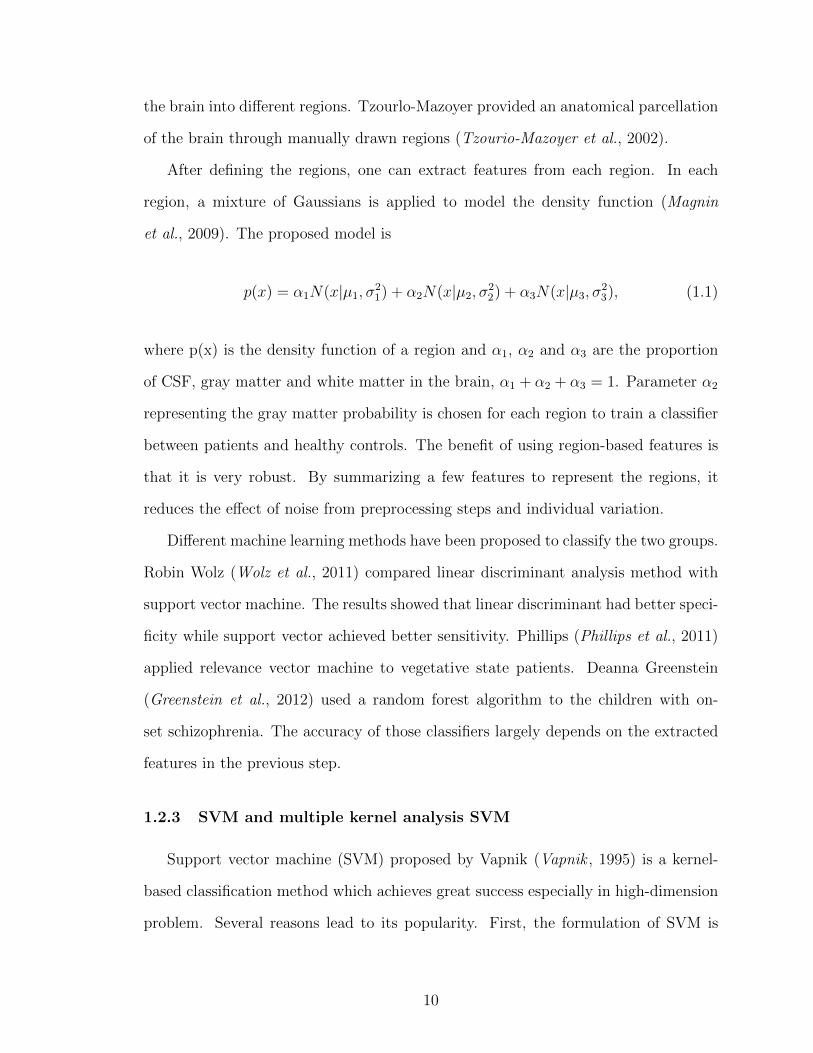
After defining the regions, one can extract features from each region. In each
region, a mixture of Gaussians is applied to model the density function (Magnin
et al., 2009). The proposed model is
p(x) = α1N(x|µ1, σ21) + α2N(x|µ2, σ
22) + α3N(x|µ3, σ
23), (1.1)
where p(x) is the density function of a region and α1, α2 and α3 are the proportion
of CSF, gray matter and white matter in the brain, α1 + α2 + α3 = 1. Parameter α2
representing the gray matter probability is chosen for each region to train a classifier
between patients and healthy controls. The benefit of using region-based features is
that it is very robust. By summarizing a few features to represent the regions, it
reduces the effect of noise from preprocessing steps and individual variation.
Different machine learning methods have been proposed to classify the two groups.
Robin Wolz (Wolz et al., 2011) compared linear discriminant analysis method with
support vector machine. The results showed that linear discriminant had better speci-
ficity while support vector achieved better sensitivity. Phillips (Phillips et al., 2011)
applied relevance vector machine to vegetative state patients. Deanna Greenstein
(Greenstein et al., 2012) used a random forest algorithm to the children with on-
set schizophrenia. The accuracy of those classifiers largely depends on the extracted
features in the previous step.
1.2.3 SVM and multiple kernel analysis SVM
Support vector machine (SVM) proposed by Vapnik (Vapnik , 1995) is a kernel-
based classification method which achieves great success especially in high-dimension
problem. Several reasons lead to its popularity. First, the formulation of SVM is
10

intuitive and easy to understand. Second it is a kernel-based method which is flexible
with a broad range of problems. Third it suits small sample and high dimension
problems well. As in the VBM case, SVM was used in the function MRI to predict
the state of the scans during a block design experiment (LaConte et al., 2005). Then
it was proposed for structural MRI, achieving good results in various kinds of data.
Lao (Lao et al., 2004) first applied the SVM to the structural MRI to determine the
gender of the subjects. The study showed that SVM could easily distinguish the two
groups, achieving a classification accuracy of 97%. Kawasaki (Kawasaki et al., 2007)
applied SVM to classify the schizophrenia patients from the healthy controls. Kloppel
(Kloppel et al., 2008) successfully distinguished the Alzheimer’s patients from normal
people with an accuracy of 89%.
The performance of SVM relies on the kernel which is determined before seeing
the data. Selecting a kernel and its parameters is an important issue in training. The
classical way is to use cross-validation procedure which requires an extra validation
set. However, in a small sample problem, extra data are usually hard to acquire.
Multiple kernel learning (MKL) is proposed to automatically select the best kernel.
It takes a weighted sum of different kernels instead of using a single one (Lanckriet
et al., 2004), (Sonnenburg et al., 2006). Since the weight of each kernel is automat-
ically determined by the MKL algorithm, it does not need extra data to select the
best kernels. There are two uses of MKL (Gonen and Alpaydin, 2011). First one is
to get a kernel as a combination of pre-defined kernels. Different kernels correspond
to the similarity between two subjects in different spaces and MKL finds the best
combination of all these spaces instead of just picking one. Second one is to get a
kernel as a combination of different sources. Different variables can have different
measures and can be best represented through different features. In such a case de-
signing different kernels for different variables and combining the kernels later are a
way of using multiple information sources. This means that different variables may
11

contribute to the classifier in different ways. This is intermediate combination (com-
bining kernels taken different data), different from early combination (combining the
data at feature extracting step, single kernel SVM) and late combination (combining
different classifiers taken different data) (Noble, 2004).
The latter usage can be used in the classification problem of the brain image
data. Human brain exhibits both segregation and integration properties (Kinser
and Grobstein (2000)). Segregation means that different aspects of the behaviors are
usually performed by anatomically and functionally distinct areas. Integration means
that these functionally specialized areas need to communicate with each other to
complete any tasks. These localization and globalization property of the brain can fit
in the framework of MKL method which extracts information from different local areas
and then combines them together to get a better result. In this work, we present and
evaluate a classification method based on MKL SVM. The purpose is to distinguish
the patients with a certain disease from the healthy control subjects through the
analysis of their anatomical brain images. In addition, we are also interested in the
identification of significant regions associated with a particular disease.
1.3 Overview
The material presented in this thesis covers both the fMRI analysis and structural
MRI analysis, including theoretical and practical backgrounds, simulation and real
data analysis.
Chapter II devotes to the fMRI analysis. Section 2.1 listed some characters of
fMRI data and define the purpose of fMRI studies. We also presented several chal-
lenges fMRI data bring to the statistical analysis in this section. Section 2.3 reviews
the general linear method with its ways of modeling the haemodynamic response
function and dealing with temporal and spatial correlation in the data. In section
2.4 we first explain the intuition of ICA and then dig into the details of its algorithm
12

and application. Section 2.5 gives a description of Gaussian process and the decom-
position model that we proposed to model the temporal dependent data. We applied
the proposed method to a simulated data and the results show that the estimates of
the parameters are stable around the truth. In section 2.6, we apply our model to an
auditory stimulation data set and compare our results to GLM and ICA.
Chapter III covers the analysis of structural MRI. In section 3.2, we describe
the voxel-based method, along with its preprocessing steps and statistical tests. In
section 3.3, we focus on the mathematical formulation of MKL SVM. We introduce
both the primal and dual forms of the problem which can show the benefits of these
segregating and integrating procedures. In section 3.4, we compare the results of
traditional SVM and MKL SVM in simulated data. The simulation results show that
MKL SVM can achieve a better classifier and identify the informative variables from
the noise variables. In the section 3.5, We propose a two-step MKL procedure to deal
with highly correlated areas in the brain. We apply the method to four data sets,
showing that the MKL SVM can outperform the traditional SVM in some conditions.
We also discuss some common feature selection and tuning selection issues in the real
data analysis.
13

CHAPTER II
Functional MRI Analysis
14

2.1 Introduction
Functional Magnetic Resonance Imaging (fMRI) provides a non-invasive way to
study neural activity in human brain. It is known when local nerve cells are active,
there is an increase of local blood flow after an approximately 1-5 second delay (Roy
and Sherrington, 1890). This leads to local changes in blood oxygen level which are
reflected as an increase of magnetic resonance signals (Ogawa et al., 1990). fMRI
uses this blood oxygenation level dependent (BOLD) contrast to study local neural
activity in the brain. During a typically fMRI experiment, subjects are asked to
perform a certain task while been scanned repeatedly. Each scan is a 3-D image of
the whole or a part of the brain. A typical fMRI scan has a spatial resolution of
about several millimeters (usually 3× 3× 3 mm3) and time resolution of about a few
seconds (usually 2 seconds). It is known that different areas of brain are associated
with different functions, such as analyzing sensory data, performing memory functions
and making decisions. The goal of activation analysis is to find the activated area of
the brain when the subject is performing a certain task.
The most widely used statistical method is the general linear model (Friston et al.,
1995b) which builds a linear model between the recorded signal and the expected
activation signal. Since the local blood flow usually does not synchronize with the
stimuli, the expected activation signal is represented by a convolution model between
the time course of the stimuli and the HRF. The general linear model method assumes
the observed signal is a linear function of the expected signal plus some random noise.
Then a statistical test is applied to every voxel to test whether the linear association is
significant or not. The significant regions are the active areas invoked by the stimuli.
The statistical analysis of fMRI data is challenging due to several reasons. First,
the precise mechanism linking BOLD signal and neural activity is not clear, which
means the shape of HRF is not known. Second a standard fMRI study produces
massive amounts of data, with strong temporal and spatial correlation. Further, the
15

signal we are interested in is weak in comparison to the noise which can come from
several sources, like head movement, equipment, effect of respiration and heartbeat.
The signal intensity in a given voxel typically varies by approximately 5% around the
mean during cortical task activation.
One solution to avoid the use of HRF is independent component analysis (Bell
and Sejnowski , 1995) which decomposes the recorded signal into several independent
components. This method does not assume any relation between the observed sig-
nal and the activation signal in the model estimation step. Instead, it assumes the
recorded signals are a linear combination of independent components and the goal
is to retrieve the original sources. The components with high correlations with the
stimuli are the activation sources. And the regions relies mostly on the activation
sources are the active regions invoked by the stimuli. The difficulty with this method
lies in the interpretation of the independent components and the activation regions.
In general linear model, the temporal correlation of the signal is usually modeled
by an autoregressive model for every voxel. The order of the autoregressive is fixed
for all the voxels across the brain. However, the strength of the temporal correla-
tion varies for different regions. Gaussian process is a good method to model the
stochastic process with temporal correlation. Gaussian process is a stochastic process
for which any collection of finite variables follow a multivariate Gaussian distribution
(Rasmussen and Williams , 2006). One advantage of Gaussian process is its flexibil-
ity in designing the level and the structure of the correlation through the covariance
matrix. We explore this advantage and design a Gaussian process model to model
the fMRI signal.
The rest of this chapter provides more details of statistical methods on fMRI data.
We first describe the preprocessing steps that are part of standard procedure now.
We review two popular methods, general linear model and independent component
analysis. Then we propose a new decomposition method using Gaussian process. We
16

show that our model can recover the activation signal, the temporal correlated signal
and the random noise in a simulated study. We then compare our model to other
methods in a real data analysis.
17
2.2 Preprocessing
Most brain image analyses are voxel-based, relying on the voxel-wise signals to
find the regional effects in the data. This requires all the scans to be in the same
space with same voxel indicating same location across multiple scans. To meet this
requirement, a series of preprocessing steps, including realignment, spatial normal-
ization and spatial smoothing, are usually carried out before the analysis to make the
statistical assumptions valid.
Realignment Signal changes in one voxel of one session can arise from head motion
of the subject. In extreme cases, the movement can account for up to 90% of the total
noise (Friston et al., 1996b). A typical fMRI scan has a spatial resolution of 2mm but
the subjects usually show displacements of up to several millimeters. The time series
of voxel i may be contaminated by voxel j, a few millimeters away. So before dealing
with the variability between different sessions and different subjects, a realignment
procedure is applied to all the scans to eliminate the within session variability. The
Realignment involves a rigid-body transformation, minimizing the differences between
each successive scan and a reference scan. Then the transformation is applied to each
scan and a re-sampling scheme is carried out to get the signal on the grid. The results
are a series of scans aligned to the same space. Sometimes, non-linear transformation
is applied to account for non-linear effects.
Spatial Normalization Realignment reduces the within-session differences among
a series of scans. But different subjects have different brain morphometries which
must be taken into consideration before statistical analysis. Spatial normalization is
the step that maps all the scans to a same template image (Friston et al., 1995a). After
the realignment step, a mean image of the series or a structural image is used to esti-
mated the warping function that maps it onto a template (Talairach and Tournoux ,
18

1988). In practice, most people use a spatial basis function to minimize the difference
between the two images. After spatial normalization step, all the scans in the study
are in the same space in which voxels lie in the same location across different scans.
Spatial Smoothing After the spatial normalization steps, images are usually smoothed
by convolving with a Gaussian kernel. For fMRI data, the signal of interests is usually
very weak comparing to the noise. Smoothing reduces the noise, improving the signal
to noise ratio. Another reason is that smoothing makes the errors more Gaussian, an
assumption in the statistical analysis.
2.3 General Linear Model
Friston et al. (1995b) used the general linear model (GLM) for activation analysis.
In their work the time series of each individual voxel is modeled independently as a
linear combination of the experiment-related signals and white noise. Let X(t) be
the time series at any voxel, then
X(t) = β0 + β1g1(t) + β2g2(t) + . . .+ βKgK(t) + ε(t), (2.1)
where gk is the explanatory variable relating to the k-th experiment condition. Putting
equation (2.1) in matrix form
X = Gβ + ε, (2.2)
where X is the observed time series at a specific voxel. Matrix G is the design matrix
with columns gk. ε is the white noise ε ∼ N (0, σ2I).
The covariate gk(t) is the expected BOLD signal corresponding to the k-th exper-
imental condition. The BOLD signal evoked by a single stimulus is referred to as the
haemodynamic response function (HRF). Due to the sluggish nature of the HRF, the
BOLD signal is not a linear function of stimulus function. A common way to model
19

BOLD signal is through a linear time-invariant model.
Let uk(t) be the time series of stimulus of condition k and h(t) be the HRF,
linear time-invariant model expresses BOLD signal as the convolution of the stimulus
function and HRF (Boynton et al., 1996).
gk(t) = uk(t)⊗ h(t) =
∫uk(t− τ)h(τ)dτ. (2.3)
There are usually two types of experimental design, epoch and event-related, which
lead to different expressions of function u(t). In epoch model, uk(t) is a boxcar
function, with value 1 at the time when condition k is on and 0 otherwise,
u(t) =J∑j=2
I(tj−1,tj)(t),
where I(t) is an indicator function and (tj−1, tj) is the j-th block when the stimulus
is on. Although block design is efficient in detecting the activated area, it only
measures the magnitude of BOLD signal. In event-related design, uk(t) is a stick
function (Zarahn et al., 1997):
u(t) =J∑j=1
δ(t− tj), (2.4)
where (t1, . . . , tJ) is the time series of J stimuli and δ(t) is the Dirac delta func-
tion. Event-related design is usually used to characterize transient haemodynamic
responses to brief stimuli (Josephs and Henson, 1999). It facilitates an evaluation of
the exact form of the HRF.
GLM is a massive univariate model which involves two-step analysis. First linear
model (2.2) is applied to each time series separately. Then a test statistic (usually T-
statistic or F-statistic) of the null hypothesis that there is no activation for condition
20

k is computed for each voxel,
H0 : βk = 0 H1 : βk > 0.
This creates a statistical image with each voxel represented by its corresponding test
statistic. At the second level of analysis, a threshold for test statistic is chosen based
on some multiple testing correction techniques such as random field theory (RFT)
and false discovery rate method (FDR).
GLM is the dominant method to analyze fMRI data mainly due to its compu-
tational simplicity. There are several issues about this method. First it fails to
accommodate the spatio-temporal correlation in the data. The temporal correlation
is due to the sluggish nature of BOLD. The spatial correlation can come from several
sources, like image reconstruction and preprocessing steps. Second, it performs a
extremely large number of tests simultaneously (usually on the scale of 100000) with
multiple comparison issues. Third, the power of GLM strongly depends on the form
of the HRF. It has been observed that the exact form of the HRF varies across dif-
ferent regions of the brain. Fixing the form of the HRF largely reduces the flexibility
of the model. New methods have been proposed to deal with above issues.
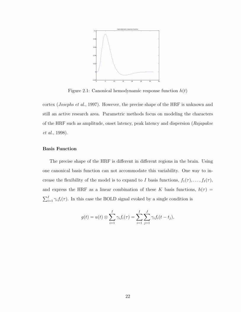
2.3.1 HRF
The mechanism between neural activity and BOLD signal is complicated and only
partially understood. A typical HRF, the BOLD response to a single stimulus, usually
peaks approximately 5s after stimulation, and is followed by an undershoot that lasts
as long as 30s, as showed in Figure 2.1.
This canonical HRF is widely used as a basis function in (2.3). Empirical studies
show that the shape of the HRF is similar across sensory regions in brain, for example
motor cortex (Aguirre et al., 1998), visual cortex (Boynton et al., 1996) and auditory
21
0 5 10 15 20 25 30 35−0.02
0
0.02
0.04
0.06
0.08
0.1haemodynamic response function
Figure 2.1: Canonical hemodynamic response function h(t)
cortex (Josephs et al., 1997). However, the precise shape of the HRF is unknown and
still an active research area. Parametric methods focus on modeling the characters
of the HRF such as amplitude, onset latency, peak latency and dispersion (Rajapakse
et al., 1998).
Basis Function
The precise shape of the HRF is different in different regions in the brain. Using
one canonical basis function can not accommodate this variability. One way to in-
crease the flexibility of the model is to expand to I basis functions, f1(τ), . . . , fI(τ),
and express the HRF as a linear combination of these K basis functions, h(τ) =∑Ii=1 γifi(τ). In this case the BOLD signal evoked by a single condition is
g(t) = u(t)⊗I∑i=1
γifi(τ) =I∑i=1
J∑j=1
γifi(t− tj),
22

where u(t) is an event-related design and takes the form of (2.4). Having specified
the form of stimulus and the HRF, equation (2.1) can be written as
X(t) =K∑k=1
βkgk(t) + ε(t)
=K∑k=1
βk
I∑i=1
J∑j=1
γifi(t− tkj) + ε(t)
=K∑k=1
I∑i=1
J∑j=1
αkifi(t− tkj) + ε(t),
where αki = βkγi and (tk1, . . . , tkJ) is the time series of stimulus function for the k-th
condition. A common choice for function (f1(t), . . . , fI(t)) is based on the canonical
HRF and its partial derivatives. The canonical HRF can be characterized by the
difference between two gamma functions, one modeling the peak and the other mod-
eling the undershoot. Derivative function can capture the difference in onset latency
among different brain regions.
Another popular set of basis functions is three gamma density functions with mean
and variance both setting to 2i (i = 2, 3 and 4). They can be seen as functions peaking
during the early, intermediate and late components of the anticipated haemodynamic
response. And also derivatives of these three basis functions are used in the case when
there is temporal delay effect. Figure 2.2 plots the basis functions.
0 5 10 15 20 25 30 35−0.1
−0.05
0
0.05
0.1
0.15
0.2
0.25Basis Functions and Derivatives
Figure 2.2: Basis function fk(t) and its derivatives
23

2.3.2 Temporal Correlation
Purdon and Weisskoff (1998) investigated the temporal correlation in fMRI data.
A simulation study demonstrated that the false-positive rate can be biased far above
or below the significant level if the actual autocorrelation was ignored. Instead of
assuming independence along the time series, they proposed a new method using
first-order autoregressive (AR(1)) model to accommodate the temporal correlation
in noise term. The error term ε(t) in (2.1) is modeled as a sum of AR(1) series and
white noise,
ε(t) = z(t) + δε(t)
z(t) = az(t− 1) + δz(t),
where δε(t) and δz(t) are independent Gaussian, δε(t) ∼ N (0, σ2ε ), δz(t) ∼ N (0, σ2
z).
a is the AR(1) coefficient. Then the resulting covariance matrix is
E(εεT ) = σ2z(I− A)−1(I− A)−T + σ2
ε I,
where A is a matrix with all elements of the first lower off-diagonal set to a and zero
elsewhere. I is the identity matrix of dimension T .
2.3.3 Multiple Testing Correction
Correction for multiple testing is crucial for the interpretation of activation anal-
ysis. A typical fMRI experiment produces massive amounts of voxels with strong
spatial correlations. The reasons for spatial correlation come from different sources,
such as image reconstruction, physiological signal and spatial preprocessing. Since
the BOLD signal is relatively low comparing to noise, the standard preprocessing step
involves smoothing along the spatial direction, usually with a Gaussian kernel of full
24

width at half maximum (FWHM) of 8 pixels. At the modeling level, GLM assumes
independence among voxels and fits each time series individually. This spatial corre-
lation is addressed in inference step through multiple testing correction technique.
Bonferroni Correction
There are several methods to address the multiple comparison issue. One way is to
control the family-wise error rate (PFWE) using Bonferroni correction. The significant
level α for an individual test is then
α = PFWE/N,
where N is the number of individual tests (number of voxels in brain). However, in
standard fMRI experiment, we deal with about 100000 multiple tests simultaneously.
The Bonferroni correction is too conservative. Further scans have spatial correlation
which makes the effective degree of test statistics much smaller. Usually Bonferroni
correction does not lead to correct family-wise error rate.
Random Field Theory
This spatial dependence problem can be corrected using random field theory
(RFT) (?). The way that RFT solves this problem is through expected value of
Euler Characteristic (EC) for a smooth statistical map. Euler Characteristic is de-
fined as the number of clusters of voxels that exceed a given threshold in the brain
volume (Worsley et al., 1996).
False positive rate is the probability of at least one voxel activated which is equiv-
alent to the largest Z value in one region is above some threshold. This is the same
as the probability of finding at least one region above the threshold. And at high
thresholds the EC is either is zero or one. so we have the probability of a family-wise
25

error is approximately equivalent to the expected Euler characteristic:
PFWE = P(Zmax > Zα) = P(EC ≥ 1) ≤ E(EC).
False Discovery Rate
Instead of controlling type I error, false discovery rate (FDR) approach tries to
control the expected proportion of false positives among those tests detected as pos-
itive (Benjamini and Hochberg , 1995). The algorithm is to calculate the p-value for
each individual voxels and order them, p1 ≤ p2 ≤ . . . ≤ pN . To control FDR at
level α, the largest k which satisfies pk < αk/N was found. Then tests associated
with p1, . . . , pk are considered as positive. FDR approach shows higher power than
Bonferroni correction in fMRI data set (Genovese et al., 2002). The resulting thresh-
old chosen by FDR depends on the amount of significant signals in the data set not
on the number of voxels or the smoothness in the data. So unlike single choice of
threshold across data sets, FDR method adapts its threshold to the features of the
data. On the other hand, ignoring the smoothness in the data sets, FDR tends to be
more conservative as the spatial correlation increases. Hence, it has higher power for
unsmoothed data while RFT typically has higher power for smoothed data.
2.4 Independent Component Analysis
GLM requires a priori knowledge about the exact form of the HRF. In the brain
regions where the HRF is quite different from the canonical form, GLM can not detect
the activation area. McKeown et al. (1998) proposed a novel approach which does
not specify the shape of the HRF. The method is based on independent component
analysis (ICA) (Bell and Sejnowski , 1995). Like PCA, ICA decomposes a time series
of scans into a linear combination of several sources and associated weights. But
unlike PCA which tries to find the best solution in terms of minimizing the mean-
26
square error, ICA decomposes the original signals into components as independent as
possible.
2.4.1 Definition of ICA
Let X1, . . . , XJ be J random variables. ICA assumes that each random variable
can be decomposed into a sum of independent random variables. The mixture Xj is
a weighted linear combination of K independent components S1, S2, . . . , SK :
Xj = aj1S1 + aj2S2 + . . .+ ajKSK . (2.5)
Let X = (X1, . . . , XJ)T be the random vector of mixtures and S = (S1, S2, . . . , SK)T
be the random vector of independent components and A be the mixing matrix with
elements ajk with j ∈ {1, 2, . . . , J} and k ∈ {1, 2, . . . , K}. Then (2.5) can be written
in matrix form:
X = AS. (2.6)
All we observed is the mixtures X. Both the hidden variables S and the mixing
matrix A need to be estimated. Assuming A is a square matrix which means we
have same number of mixing signals and independent components, we can write (2.6)
the following way:
S = WX,
where W = A−1 is the inverse of the the mixing matrix. ICA estimates the inverse
of mixing matrix by maximizing some measure of independence of (S1, S2, . . . , SK)T .
2.4.2 ICA for fMRI
There are two types of ICA methods applied to fMRI data, spatial ICA (sICA)
and temporal ICA (tICA). sICA assumes the brain areas activated by performance
of a certain task should be unrelated to the brain areas whose signals are affected by
27

artifacts, such as physiological pulsations, subtle head movements and machine noise.
At each time point t, sICA decomposes images of the brain X(t) = (x1(t), . . . , xN(t))
into K independent components
X(t) = a1(t)S1 + a2(t)S2 + . . .+ aK(t)SK , (2.7)
where Sk = (sk1, . . . , skN) is a N-dimension brain image. The coefficients, ak(t)
t = 1, . . . , T , are considered as the activation time series associated with the k-th
component. Equation 2.7 implies the change of the observed signal X(t) results from
a change in the relative contribution from each component other than from component
itself. Activation component is found by computing the correlation between the time
series of independent components and a reference function, usually the time course
of stimuli and or the expected BOLD signal. The underlying argument is the same:
the activated voxels share a similar time course as neural activity.
The activated map is the component whose associated time course has the highest
correlation. The voxels with the highest weights on the activated map are considered
as activated regions. McKeown et al. (1998) first applied sICA to fMRI data and
argued that there were spatial independence among consistently task-related fMRI
activation (the components that were highly correlated with the reference function),
transiently task-related fMRI activation (the components that were correlated with
the reference function during part of the trial), slowly varying components (regions
of ventricular system), head movement (the components that have abrupt changes in
their time courses), quasiperiodic components (signals might be caused by aliased car-
diac and respiratory rhythms) and noise components. It also argued that maps of the
activated voxels for task-related components contained areas of activation resembling
those produced by computing the correlation between observed signal and reference
function. In addition, ICA method detected other area that have not detected by the
28
correlation method.
tICA assumes that the time series of each individual voxel can be decomposed
into linear combination of independent times series. For each voxel n, tICA mod-
els the time series Xn = (Xn(1), . . . , Xn(T )) as a linear mixture of K independent
components (S1, . . . , SK)
Xn = an1S1 + an2S2 + . . .+ anKSK ,
where Sk = (sk(1), . . . , sk(T )) is a T -dimension time series. The coefficients, ank,
n = 1, . . . , N is the brain map associated with the k-th component. The activation
component is the one with the highest correlation with the reference function. Then
activation area can be found by inference about the brain map associated with the ac-
tivation component. Biswal and Ulmer (1999) used tICA to decompose the observed
signals into different identifiable individual sources, such as task-related components,
cardiac and respiratory pulsations.
Assuming spatial or temporal independence of fMRI data yields two different
interpretation of the ICA method. sICA has dominated the application of fMRI.
One possible explanation is that standard ICA algorithm needs whitening the data
first which projects the mixed signals onto a much smaller K-dimension space. Since
in fMRI data set, the spatial dimension (about 100000 voxels) is much larger than
temporal dimension (usually 200-300 scans), the preprocessing step for tICA loses
too much information about the original data. Calhoun et al. (2001) examined these
two different approaches. Results showed that sICA and tICA tended to have similar
results given components were independent in both space and time and diverged if
the components were highly correlated in space or time. It was shown that if there
was one single experimental design, both sICA and tICA can separate the BOLD
signal from other sources (Petersen et al., 2000). So whether applying sICA or tICA
29

should depend on the question whether the expected BOLD signals or hypothesized
activated areas are heavily dependent.
Several questions need to be addressed before applying ICA. First, the number
of independent components we want to extract has to specify before. The results
depend heavily on the choice of K and there is no natural ordering of independent
components. The standard algorithm sets the number of independent components
the same as the number of observed signals. Second, the interpretation of other
independent components is not clear. Third, there are several algorithms proposed to
find independent components based on different contrast functions. Applying different
algorithm might lead to different activation areas. Several popular algorithms are
explained briefly in the following sections.
2.4.3 Identifiability Issues
Comon (1994) addressed the identifiability issue of ICA. First, the number of
observed mixture signals must be at least as large as the number of independent
components. To identify A and S, we have to put a further constraint that var(Sk) =
1. Since any orthogonal transformation of independent Gaussian variables is also
independent, another fundamental assumption in ICA model is that independent
components should be non-Gaussian. In order to uniquely determine the independent
components, we need the following conditions:
• Sk for k = 1, 2, . . . , K are non-Gaussian, with possible exception of at most one
component.
• var(Sk) = 1 for k = 1, 2, . . . , K.
• The number of mixing signals should be no less than the number of independent
components, J ≥ K.
30

With these constraints, the mixing matrix A and the hidden variables S can be
identified up to a permutation matrix (Hyvarinen and Oja, 2000).
2.4.4 Measures of Independence
All ICA algorithms are based on the optimization of some measures of indepen-
dence of S. Popular algorithms used in fMRI data analysis are Infomax (Bell and
Sejnowski , 1995), JADE (Cardoso and Souloumiac, 1993) and FastICA (Hyvarinen
and Oja, 2000). The performance of different algorithms depends on how well the
data’s high order structure matches the assumptions of the algorithm. Infomax al-
gorithm works well for sICA (McKeown et al., 1998). However, when the Infomax
algorithm looked for temporally independent waveforms, it was less efficient because
the boxcar design of the experiment doesn’t match its implicit assumption about the
underlying distribution. (McKeown et al., 2003).
Maximum Likelihood Approach
One possible way to estimate both independent sources S and mixing matrix A is
to take a maximum likelihood approach Pham and Garat (1997). Under model 2.5,
the likelihood of the observed signal can be written as
L(A,x) =N∑n=1
K∑k=1
log pk(wkxn) +N log | det(W)|
=N∑n=1
K∑k=1
log pk(eTkA−1xn) +N log | det(A−1)|.
The likelihood estimate of A is the value that maximizes L(A,x).
Information Maximization
Bell and Sejnowski (1995) took an information-maximization (Infomax) approach.
This approach is based on maximizing the entropy of a non-linear function of the inde-
31

pendent sources, Let H be the entropy function, a direct computation of H(S1, S2 . . . , SK)
gives
H(S) = −∫
P(S) log P(S)dS
= −∫
P(X) logP(X)
| det W|dX
= H(X) + log | det W|.
So without any regulation, H(S) diverges to infinity for an arbitrary large W.
Thus, Infomax approach considers entropy of some contrast function g, which is
usually an increasing function mapping from R to [0, 1]. The algorithm finds the
estimates of S that maximize H(g(S1),g(S2), . . . ,g(SK)).
Let random variable Vi be a random variable whose cumulative distribution func-
tion is g. Let V = (V1, V2, . . . , VK) and U ∼ Unif [0, 1]K . Then the entropy of the
contrast function of hidden components is:
H(g(S)) = −Eg(S) log P(g(S)) (2.8)
= KL(g(S)||U)
= KL(S||g−1(U))
= KL(S||V).
This shows the Infomax approach is equivalent to the minimization of the Kullback-
Leibler (KL) distance between the independent resources S and the distribution
associated with g. A popular choice of contrast function g is logistic function,
g(s) = (1 + e−s)−1 (Bell and Sejnowski , 1995).
Cardoso (1997) shows if the contrast function g is chosen as the cumulative distri-
bution function of S, infomax is equivalent to maximum likelihood estimation. The
maximum likelihood approach can be written as a KL distance between two distri-
32

butions:
arg maxL(A,x) =1
Narg max
A
N∑n=1
log P(Xn|A)
= arg maxA
∫P∗X log P(X|A)dX
= arg maxA−KL(P∗X||P(X|A))−H(P∗X)
= arg minA
KL(P∗(S|A)||P(S)),
where P∗X is the empirical distribution of X and P∗(S|A) is the empirical distribution
of S given mixing matrix A. So, if the contrast function g in (2.8) is chosen to be
the cumulative distribution function of S, then the maximum likelihood method is
the same as Infomax approach. In the infomax approach, any contrast function g
mapping from R to [0, 1] is chosen as the cumulative distribution function of the
independent sources which need to be estimated in the maximum likelihood method.
Mutual Information and Kullback-Leibler divergence
Comon (1994) used mutual information as a measure of dependence. The mutual
information I of K random variables Y = (Y1, Y2, . . . , YK) is defined by the following
equation:
I(Y1, Y2, . . . , YK) =K∑k=1
H(Yk)−H(Y).
Mutual information can be interpreted as the a measure of the information that
Y1, Y2, . . . , YT share. It is always non-negative and is zero if and only if (Y1, Y2, . . . , YT )
are independent. So the ICA estimate of the problem 2.6 using the mutual information
is:
arg minA
I(eT1 A−1X, eT2 A−1X, . . . , eTKA−1X).
Since the entropy depends on the unknown distribution of S, the maximization
of the mutual information needs the approximation of the density function. Comon
33

(1994) used Gram-Charlier expansion which is a polynomial density expansion based
on higher-order cumulants. For random variable Y of zero mean and unit variance,
the Gram-Charlier expansion is
P(y) ≈ φ(y)(1 + κ3(Y )h3(y)/6 + κ4(Y )h4(y)/24 + . . .),
where φ is the Gaussian density function. κi(Y ) is the i-th cumulants of the random
variable Y and hi(y) are Hermite polynomials defined recursively:
h0(y) = 1
h1(y) = y
hn+1(y) = yhn(y)− h′n(y)
Plugging the estimate of the density function, we get the mutual information of
S = (s1, s2, . . . , sK), under the constraint that (s1, s2, . . . , sK) are uncorrelated. We
have:
I(S) = C +1
48
K∑k=1
(4κ3(sk)2 + κ4(sk)
2 + 7κ4(sk)4 − 6κ3(sk)
2κ4(sk)), (2.9)
where C is a constant and κi(sk) is the i-th cumulant of empirical distribution P∗k of
sk.
Since the Gram-Charlier expansion is based on Taylor expansion of density func-
tion at the point of Gaussian density function, the approximation is valid if the true
distribution is not far from Gaussian. Then the estimate achieves the minimum of
(2.9).
34

Kurtosis
One-contrast function method allows the estimation of one independent compo-
nent at each time. Instead of maximizing some measures of mutual independence,
one-contrast function method tries to maximize the measure of non-Gaussianity for
each component Sk. In many applications, we are only interested in a few compo-
nents. So it is not necessary to extract K independent components at the same time
(Hyvarinen, 1999). And estimation of one component at one time greatly reduces the
computation complexity.
From the projection pursuit point of view, the decomposition of J signals into a
weighted sum of K components is to project high dimension data onto a lower space.
It has been argued that Gaussian distribution is the least interesting structure in
terms of the information it carries. So the projection should be in the least Gaussian
direction. One-contrast function method uses the same idea trying to find the least
Gaussian projection at each time.
The classical measure of non-Gaussianity is kurtosis. The kurtosis of random
variable Y is the fourth cumulant:
Kurt(Y ) = E(Y 4)− 3(E(Y 2))2.
If Y has unit variance, then Kurt(Y ) = E(Y 4) − 3 is a normalized version of the
fourth moment. For standard Gaussian variable z, Kurt(z) = 0. For most non-
Gaussian variables kurtosis is nonzero. Kurtosis is widely used as a measure of non-
Gaussianity. The main reason is its linearity property which makes both theoretical
and computational analyses easier. For independent variables Y1 and Y2 with zeros
means and unit variances,
Kurt(c1Y1 + c2Y2) = c41Kurt(Y1) + c42Kurt(Y2).
35

Let w be a row vector in the inverse mixing matrix W. Then wX is the estimate of
one component. The kurtosis approach tries to maximize the kurtosis of the estimated
component,
maxw|Kurt(wX)| = max
w|Kurt(wAS)|
= maxc|Kurt(cS)|
= maxc|K∑k=1
c4kKurt(Sk)|,
where c = wA. Since we assume that var(Sk) = 1 for k = 1, 2, . . . , K, we get∑Kk=1 c
2kvar(Sk) =
∑Kk=1 c
2k = 1. So the optimization problem becomes
maxc|K∑k=1
c4kKurt(Sk)| with the constraintK∑k=1
c2k = 1, (2.10)
If we assume there is at least one component whose kurtosis is negative and at
least one whose kurtosis is positive, the maximum in (2.10) is achieved at c = ±eTj ,
where ej is a column vector with 1 on the j-th row and 0 elsewhere (Delfosse and
Loubaton, 1995). Then wX = ±eTj A−1X = ±eTj S. This means maximizing the
contrast function gives us the independent component Sj up to a sign difference.
Since the measure of non-Gaussianity is based on the fourth cumulant, the kurtosis
approach is very sensitive to outliers.
Negentropy
Negentropy is a natural choice to assess the distance between Gaussian distribu-
tion and any other distribution. Let J be the negentropy of any random vector S,
negentory of J is defined as
J(S) = H(Sgauss)−H(S),
36

where Sgauss is a Gaussian random vector which has the same mean and covariance
matrix as S. Negentropy is non-negative and achieves 0 if and only if S is Gaussian.
It is invariant to any linear transformation.
There is a natural link between negentropy and independence through mutual
information. The Mutual information can be expressed in terms of negentropy,
I(S1, S2, . . . , SK) = J(S)−K∑k=1
J(Sk) +1
2log
∏Kk=1 Σkk
det(Σ)|, (2.11)
where Σ is the covariance matrix of S and Σkk is its k-th diagonal element. If
(S1, S2, . . . , SK) are uncorrelated then (2.11) becomes
I(S1, S2, . . . , SK) = J(S)−K∑k=1
J(Sk).
In the ICA model (2.6), the negentropy of S is the same as the negentropy of
X which does not depend on W. Maximizing independence is the same as mini-
mizing mutual information and also the same as maximizing the sum of negentropy.
Assuming S1, S2, . . . , SK are uncorrelated,
arg minA
I(S) = arg maxw1,...,wK
K∑k=1
J(Sk)
= arg maxw1,...,wK
K∑k=1
J(wkX),
with the constraint that (w1,w2, . . . ,wK) are linearly independent where wk is the
k-th row in the inverse mixing matrix W. Negentropy of S depends on the un-
known distribution of S. Different approximations were proposed based on different
assumptions of the underlying distribution. Jones and Sibson (1987) used Gram-
Charlier expansion as an approximation of density function to compute negentropy.
37

Given S is of zero mean and unit variance, the negentropy has the following form:
J(S) ≈ 1
12κ3(S)2 +
1
48κ4(S)2,
where κ3 and κ4 are the third and fourth cumulants of S. This approximation is also
a polynomial function of cumulants. It has been argued that these cumulant-based
methods often provide a poor approximation of entropy since higher order cumulants
are quite sensitive to outliers.
Hyvarinen (1998) proposed a different approximation of negentropy. Given S has
zero mean and unit variance.
P(S) ≈ φ(S)(1 +n∑1
ciGi(S)),
where P(S) is the density function of S, φ is the standard Gaussian density function
and Gi are some regulation functions which satisfy
∫P(S)Gi(S)dS = ci for i = 1, 2, . . . , n
∫φ(S)Gi(S)Gj(S)dS =
1 if i = j
0 if i 6= j.
Then using Taylor approximation to the logarithmic function (1 + P(S)) log(1 +
P(S)) = P(S) + P(S)2/2, the approximation to negentropy is:
J(S) ≈n∑i=1
ki[E(Gi(S))− E(Gi(z))]2, (2.12)
where ki are constants and z follows a standard Gaussian distribution.
Theoretically, Gi can be any orthogonal function with respect to Gaussian distri-
bution. But in practice, the expectation of Gi(S) should be easy to compute. And
38

in order to get more robust estimate than cumulant approach, Gi(S) must not grow
faster than quadratically. Hyvarinen and Oja (2000) considered the simplest case
when n = 1. Then (2.12) becomes
J(S) ≈ [E(G(S))− E(G(z))]2.
Two possible choices for G are given, (Hyvarinen and Oja, 2000)
G1(S) =1
alog cosh aS G2(S) = − exp(−S2/2),
where a is some suitable constant, usually 1 ≤ a ≤ 2.
2.5 Gaussian Process
At the modeling level, GLM assumes spatio-temporal independence in fMRI data
which is generally not a reasonable assumption. Spatial correlation is addressed
indirectly by smoothing the data using a Gaussian kernel in the preprocessing step
and then applying Gaussian RFT to the map of test statistics. The difference in
the assumptions of two-level analysis makes standard model diagnosis not feasible.
Models that incorporate the spatio-temporal dependences are desirable. AR(1) plus
white noise model takes the temporal correlation into consideration by specifying
the first order correlation for all voxels. However, the order of temporal correlation
depends on several factors which can vary across different regions in brain. We propose
a model using the Gaussian process to accommodate this variability in temporal
correlation.
39

2.5.1 Gaussian Process for fMRI
A Gaussian process is a collection of random variables, any finite number of which
have a joint Gaussian distribution. A Gaussian process can be completely specified
by its mean function m(t) and the covariance function k(t, t′). Let f(t) be a Gaussian
process with mean function m(t) and covariance function k(t, t′),
m(t) = Ef(t)
k(t, t′) = E(f(t)−m(t))(f(t′)−m(t′)).
Then Gaussian process f(t) denotes as
f(t) ∼ GP(m(t), k(t, t′))
Neal (1998) used the Gaussian process model for both regression and classification
showing that it is a very flexible method to define prior distributions over functions.
He argued that the there are several reasons for its popularity. First, a variety choices
of covariance functions can give functions in different degrees of smoothness. Second
Gaussian process is suited for modeling of large number of correlated variables. Be-
cause of the explicit form of conditional gaussian distribution, the estimation is much
easier than other distributions. Third, it is easy to incorporate the prior information
into the Gaussian process. These advantages make Gaussian process a useful tool
for the fMRI analysis. So In our model, we proposed a different way to decompose
the signal into a long drift signal, an activation signal, a temporal correlated signal
and an independent noise. The variation in the signal were divided into the Gaussian
process and the pure noise.
Let X(t) be the time series for a specific voxel, the signal can be decomposed into
a linear combination of mean function m(t), a zero mean Gaussian process G(t) and
40

a white noise term ε(t)
X(t) = β0 + β1I(t) + β2g(t) +G(t) + ε(t). (2.13)
β0 is the parameter of the scale of time series. The intensity of fMRI image depends
on the type of tissue it measures, ranging from 0 (area outside of brain) to about
1600 (cerebrospinal fluid area). I(t) is a centered linear function which characterizes
the linear trend usually observed in fMRI signals. g(t) is the expected BOLD signal
evoked by the experimental stimulation, modeled as a convolution of stimulus function
and the canonical HRF. ε(t) is the white noise, ε(t) ∼ N (0, σ2ε I).
The termG(t) is a zero mean Gaussian process, which characterizes the temporally
correlated component in X(t), such as physiological effect and random drift due to
instability of scanner. The temporal correlation should decrease as the time lag
increases. Further it is reasonable to assume the effect of series correlation only exits
in a relative short-range and the order of this correlation varies across the different
regions of the brain. Based on the above assumption, we use an exponential covariance
matrix with two parameters σ2 and φ to characterize the Gaussian process.
G(t) ∼ GP(0, σ2 exp(−|t− t′|
φ)),
where σ2, the variance of Gaussian process, measures the amount of fluctuation.
Parameter φ controls the order of time correlation. As φ decreases, the temporal
dependence goes to 0 at a very fast rate.
The mean function of Gaussian process model (2.13) is similar to the one in
GLM. The covariance function of Gaussian process addresses the non sphericity in
fMRI data set. It decomposes the noise term in equation (2.1) into two zero mean
Gaussian components. One is a temporally independent component which is just
random noise. The other is a temporally dependent signal which can reveal some
41

information of functional regions of the brain. Since there is a parameter φ in the
covariance matrix, the estimation needs some iterative fitting techniques or sampling
methods. A simulation study is done applying both Metropolis-in-Gibbs sampler and
Expectation-Maximization (EM) method to examine whether Gaussian process can
be separated from noise term.
2.5.2 Simulation Study
Time series with a length of 240 is generated from (2.13) with six parameters
chosen to match the real data. The scale parameter, β0 = 600, reflects the intensity
of signals of grey matter in the brain. The linear trend parameter, β1, is set to 0.01.
The activation parameter, β2 = 20, characterizes strong activation. Total variance
is set to be σ2 + σ2ε = 100. The simulation study shows that the performance of
evaluation of the model depends mainly on the values of two quantities, temporal
correlation parameter, φ, and ratio of two variance, κ = σ2ε
σ2 . Different combination
is investigated. φ is set at three different levels, little correlation φ = 0.1, modest
correlation φ = 1 and high correlation φ = 4.5. And κ is investigated at three levels,
noise variance dominating, κ = 4, equal variance κ = 1 and Gaussian process variance
dominating, κ = 0.25.
Metropolis-in-Gibbs sampler
For Bayesian sampler method, non-informative priors were put for all six param-
eters. Three parameters β0, β1 and β2 in the mean function are sampled by Gibbs
algorithm and three parameters φ, σ2 and σ2ε in the covariance function are sampled
by Metroplis-Hasting algorithm. Figure 2.3 shows the posterior distribution for three
mean parameters. From left to right the posterior distribution of β0, β1, β2
For φ = 1, σ2 = 50, σ2ε = 50, the posterior distributions of parameters, β0, β1 and
β2, peak around the true value. Figure 2.4 shows the posterior distribution for three
42

covariance parameters. From left to right the posterior distribution of σ2, σ2ε , φ. The
posterior distribution of parameters show reasonable estimation. From left to right
the posterior distribution of σ2, σ2ε , φ
But for small φ (φ = 0.1) the loglikelihood is a function of (σ2+σ2ε ). The algorithm
can not differentiate Gaussian process and white noise. Figure 2.5 shows the posterior
distribution of σ2 = 80 and σ2ε = 20 when φ = 0.1. From left to right the posterior
distribution of σ2, σ2ε , φ
596 597 598 599 600 601 602 603 604 6050
100
200
300
400
500
600
700
800voxel1 hist beta0
−0.06 −0.04 −0.02 0 0.02 0.04 0.06 0.08 0.1 0.12 0.140
100
200
300
400
500
600
700voxel1 hist beta2
12 14 16 18 20 22 24 26 280
100
200
300
400
500
600
700
800voxel1 hist beta1
Figure 2.3: The posterior distribution of β0, β1, β2
0 20 40 60 80 100 120 140 1600
50
100
150
200
250
300
350
400
450voxel1 hist sigma
0 20 40 60 80 100 120 140 160 1800
50
100
150
200
250
300
350
400
450voxel1 hist sigma eps
0 0.2 0.4 0.6 0.8 1 1.2 1.40
100
200
300
400
500
600voxel1 hist phi
Figure 2.4: The posterior distribution of σ2, σ2ε , φ
0 20 40 60 80 100 120 140 160 1800
50
100
150
200
250
300
350
400
450
500voxel1 hist sigma
0 20 40 60 80 100 120 140 160 1800
50
100
150
200
250
300
350
400
450voxel1 hist sigma eps
0 0.1 0.2 0.3 0.4 0.5 0.6 0.7 0.8 0.90
100
200
300
400
500
600
700
800voxel1 hist phi
Figure 2.5: The posterior distribution of σ2, σ2ε , φ
43

σ2 σ2ε φ σ2 σ2
ε φ β0 β1 β220 80 0.1 47.46 51.55 0.45 600.97 0.0267 20.2880 20 0.1 46.78 59.86 0.03 600.84 0.0102 20.2420 80 1.0 39.47 49.02 0.55 599.83 0.0125 19.5380 20 1.0 87.67 6.98 0.97 599.70 0.0229 23.3020 80 4.5 30.75 83.62 3.24 598.69 0.0173 21.5880 20 4.5 69.13 25.34 5.00 604.86 0.0287 18.13
Table 2.1: Estimation of parameters for different σ2ε and σ2
Expectation-Maximization Algorithm
Fixing the parameters of mean function, β0 = 600, β1 = 0.01 and β2 = 20 and also
the total variance σ2 + σ2ε = 100, EM algorithm is applied to time series generated
from different values of κ = σ2ε/σ
2 and φ. where σ2, σ2ε and φ are true values which
generate the data and σ2,σ2ε and φ are the estimated values by EM algorithm. The
results show that the EM algorithm can get good estimate of mean function in all the
cases. When φ is small which means there is little correlation in Gaussian process,
G(t) behaves like white noise term ε(t). Estimation technique based on distribution
can not separate these two terms well. As in the case φ = 0.1, the algorithm tends
to decompose the variance equally between σ2 and σ2ε . In the case that κ is large,
which means the variance of noise dominates, the estimation of φ becomes worse.
This could due to the reason if the strength of the Gaussian process is small, the data
can be corrupted by the noise term which leads to inaccurate estimation.
2.6 Real Data Analysis
Before statistical analysis, there are several preprocessing steps that try to reduce
noise from different sources. The major steps involved in fMRI preprocessing are slice
timing correction, realignment, coregistration of structural and functional images,
normalization and smoothing. It is typically assumed in statistical analysis that all the
voxels are collect at the same time. But the slices of brain are sampled sequentially.
44

Therefore time series of voxels in different slices are shifted relative to each other.
Slice timing correction usually uses interpolation method to shift the time series of
each voxel. The largest source of noise in any fMRI study is from head movement of
subject. When movement occurs, the signal from a specific voxel will be contaminated
by signal from neighbors. Motion correction is a rigid body transformation (shifting
and rotation) between one image and a target image (usually the first image or the
mean image). Usually this is done by minimizing some cost function that measures the
similarity between these two images. fMRI images usually sacrifice spatial resolution
to achieve a better temporal resolution. Another preprocessing step, coregistration is
to map the fMRI image to a structural image of the same subject to make inference
about activation. This is typically performed using rigid body transformation or
affine transformation (shifting, rotation and scaling). In multiple subjects analysis, it
is important that each voxel lies in the same function region to compare the results
from different subjects. Normalization attempts to register each subjects structural
image to a template brain image. Usually this is done by a nonlinear transformation
in two steps. The first step is to estimate a continuous mapping between the points in
an input image with those in the target image. Next the mapping is used to resample
the input image so that it is warped into the target image. The last step is to spatially
smooth fMRI data using a Gaussian kernel.
2.6.1 Experiment Paradigm
One data set was used to assess the performance of different methods. The data
was from an auditory stimulation experiment. The experimental paradigm consisted
of 16 blocks alternated between rest and auditory stimulation, starting from rest.
During auditory stimulation block, subject was listened to bi-syllabic words presented
binaurally at a rate of 60 per minute. 6 scans were acquired for each block with one
scan taking 7 seconds. A total 96 acquisition were made from a single subjects with
45

each acquisition with dimension 64× 64× 64. The voxel size is 3× 3× 3 mm3. The
preprocessing steps involve realignment, coregistration, normalization and smoothing.
During preprocessing, interpolation and resampling procedures were applied to each
scan which leads to new voxel size 2 × 2 × 2 mm3. The dimension of preprocessed
scan is 79× 95× 68.
2.6.2 Activation Analysis
Both GLM and ICA were applied to one slice of the auditory data set. GLM
used the canonical HRF with AR(1). Spatial ICA was used to detect the activation
area for ICA approach. Figure 2.6 shows the activation area map. The left figure
is the activation area detected by GLM with Gaussian random field correction at
5% significant level. The right figure is activation area detected by sICA. After ap-
plying sICA 95% quantile of activated map was set as the threshold to define the
activation area. These figures show a consistency between GLM and sICA. Figure
2.7 shows the area that are mostly related to the experiment. The left figure is the
area where the GLM-estimated parameters exceed the 95% quantile of the parame-
ter map. The right figure is the area where Gaussian-process-estimated parameters
exceed the 95% quantile of parameter map. The area detected through estimation of
parameters matches the activation area. Since the Gaussian process models a higher
order temporal correlation, the area detected by Gaussian process is smoother than
GLM.
Figure 2.6: Activation maps of GLM and sICA
46

Figure 2.7: Map of β1 parameter
2.6.3 Gaussian Process Results
One activated voxel and one inactivated voxel are chosen from this slice. Gaussian
process is applied to both time series separately. There are three components in
the mean function which are estimated by β0, β1 and β2. There are two random
components, Gaussian process (G(t)) and white noise (ε(t)). The estimated Gaussian
process and white noise shown in the Figure 2.8 are the conditional expectation given
all the parameters and observed signal of the activated voxels and Figure 2.9 are the
conditional expectation of E(G|X, β0, β1, β2, σ2, σ2ε , φ) and E(ε|X, β0, β1, β2, σ2σ2
ε , φ).
Figure 2.8 and Figure 2.9 illustrate the ratio between Gaussian process and white
noise. In both cases, the activation parameter β2 is well estimated.
0 20 40 60 80 100730
740
750
760
770
780
790
800voxel1 y and beta0
scale of signalobserved signallinear trendBOLD
0 20 40 60 80 100−25
−20
−15
−10
−5
0
5
10
15voxel1 other component
centered Ygaussian processnoise
Figure 2.8: Fitted components of an activated voxel. Left figure: estimated meanfunction. Right figure: estimated random components
The figure illustrates the ratio between Gaussian process and white noise. In both
cases, the activation parameter β2 is well estimated.
47

0 20 40 60 80 100815
820
825
830
835
840
845voxel3 y and beta0
scale of signalobserved signallinear trendBOLD
0 20 40 60 80 100−8
−6
−4
−2
0
2
4
6
8voxel3 other component
centered Ygaussian processnoise
Figure 2.9: Fitted components of an inactivated voxel. Left figure: estimated meanfunctions. Right figure: estimated random components
2.6.4 Parameter Maps
EM algorithm is applied to the whole slice to assess the performance of the model.
The resulting maps of six parameters are imposed on a structure image.
Figure 2.10: Maps of β0, β1, β2, imposed on structure image
The scale map (β0) (left figure in Figure 2.10) matches the structure image well
which captures the scale of different tissue. The linear trend map (β1) shows there
exits a linear trend across the whole slice. It tends to be positive outside the brain
and negative inside the brain. The standard way of dealing with this linear trend is
to subtract the mean of the whole scan at each time point. This can introduce other
confounding factor in the following analysis since this linear trend is not uniform
across the brain. The activation map (β2) shows a smooth image of activation area
which is similar to the results of GLM.
The temporal correlation map φ (left figure in 2.11) shows that most regions
have temporal correlation at order below 4. (Most φ are smaller than 2 which give
48

Figure 2.11: Maps of φ, σ2 and σ2ε , imposed on structure image
correlation exp(−4/2) = 0.1352 at order 4.) There are several regions showing high
temporal correlation which need further interpretation.
The model divides total variance into Gaussian process variance and white noise
variance. The white noise variance is relatively uniform across the whole slice. The
Gaussian process variance tends to be higher for voxels inside the brain than the
ones outside the brain. This suggests that the main source for temporal correlation
is related to cerebral blood flow.
2.7 Discussion
This chapter proposes a Gaussian process method to model the fMRI signals.
The method decomposes the observed signals into the stimulus-related components,
a Gaussian process and a white noise. The temporal correlation is modeled by the
nonspherical structure of the Gaussian process.
The parameters can be estimated either through the EM algorithm or the Metropolis-
Hasting algorithm. The simulation study shows that the model is well-defined and
the mean functions can be estimated well in all the scenarios in the simulation study.
However when the temporal correlation in the Gaussian process is weak, the Gaussian
process can not be separated from the noise. Then the estimates of parameters of
variance become unstable.
In the real data analysis, the estimates of the mean function are comparable
to the results of the GLM. The scale parameter matches the brain tissue type and
49

the activation parameter detects the same regions as GLM. Moreover, the regions
identified by Gaussian process model has smoother boundaries than GLM.
The estimates of the variance parameters show that the correlation levels vary
across the whole brain. Using the autocorrelation model with the same order for the
every voxel may not capture the temporal correlation well. The voxels with high
correlation are clustered together in the brain. Those regions need further interpre-
tation.
50

CHAPTER III
Structural MRI Analysis
51

3.1 Introduction
Structural MRI provides physicians and researchers a noninvasive method to pro-
duce high-resolution images of the brain’s anatomical structure. The pathological
changes associated with neurological and psychiatric diseases may cause loss of brain
tissue or atrophy in the brain. Structural MRI offers a way of visualization of these
brain changes in vivo by measuring the tissue density at a very fine grid. Different
methods have been proposed to analyze the structural MRI and a number of studies
have already demonstrated that MRI scans can provide biological plausible results in
various diseases (Kopelman et al., 2001), (Bottino et al., 2002) and (Shenton et al.,
1991).
In the following sections, we presented two popular methods, voxel-based method
(Wright et al., 1995) and support vector machine (SVM) (Kloppel et al., 2008) in more
details for structural MRI analysis. We discovered each method’s advantages and
limitations. Then we proposed a new method for structural MRI based on multiple
kernel SVM (Sonnenburg et al., 2006). Theoretically multiple kernel SVM is an
extension from single kernel SVM but the this extension gives more flexibility to the
method leading to a better classifier in many cases. We then study the new method
on both simulated data and real data. The performance of the method is discussed
under different scenarios.
3.2 Voxel-based Method
The traditional technique of identifying structural changes in the brain is a volu-
metric measurement method, involving manually drawing regions of interests (ROI)
and visually assessing any morphological changes in those regions (Chan et al., 2001),
(Keller and Roberts , 2009). However, as MRI scans become a standard procedure for
both clinical diagnosis and brain research, automated tools are desired to save time
52

and energy from time-consuming manual measurements and subjective assessment.
Voxel-based morphometry (VBM) is such a technique proposed by Wright in 1995
(Wright et al., 1995). This method first maps all the scans to a brain template and
then constructs a statistical test for every voxel to identify the regional differences
between the two groups. It is the counterpart of the GLM in the functional MRI
analysis and quite successful in distinguishing neurodegenerative diseases (Whitwell
and Jack , 2005).
Registeration VBM is a univariate method, comparing the values of one voxel
across multiple scans at one time. In order for the statistical tests to be valid, all
brain scans have to be registered to the same space. Then one voxel from one scan
will mean the same voxel of other scans. This step is called spatial registration which
involves a rigid body transformation (Friston et al., 1995a) and a non-linear warping
(Ashburner and Friston, 1999). The rigid body transformation optimizes an affine
transformation that maps the individual MRI scan to a template. This corrects for
the head movement of different subjects. The non-linear warping involves mapping
images of individuals into the same template through a set of basis functions. This
reduces the variability of different shapes of the brains. After registration, the scans
are aligned to the same template and a location in one scan corresponds to the
same location in another scan. However, registration also reduces the disease-related
morphometric differences between two groups which are the signals that we want to
detect in VBM.
Segmentation Some neuro-related diseases will cause the shrinkage in the volume
of gray matter and the expansion of the white matter in local regions of the brain.
Segmenting the brain into different tissues will facilitate the detection of the affected
regions and minimize the partial volume effects. One popular procedure before statis-
tical analysis is segmenting the brain into gray matter, white matter and cerebrospinal
53

fluid (Fischl et al., 2002). One way is to use K mixtures of Gaussian to model the
voxel density while building the voxel location information into the prior information
(Ashburner and Friston, 2005). This method is explained below.
Let µk and σ2k be the mean and the variance of the k-th Gaussian of the whole
brain. Let ci be the class label of voxel i, ci ∈ {1, . . . , K}. yi is the value of the i-th
voxel. Then the conditional probability of voxel i given that the voxel belongs to the
k-th Gaussian is
P (yi|ci = k, µk, σ2k) =
1
(2πσ2k)
12
exp
(−(yi − µk)2
2σ2k
).
Let γk be the mixture proportion for the k-th Gaussian,∑K
k=1 γk = 1. Rather than
assuming a stationary prior probability across the whole brain, the prior takes the
voxel location into consideration:
P (ci = k|γk, α) =γkbik(α)∑Kj=1 γjbij(α)
,
where bik is a function incorporating the tissue probability for class k at voxel i. α is
the deformation parameters of a set of spatial basis functions. Then the log-likelihood
function for a single voxel i can be written as
L(yi|µ, σ2, γ, α) = log
(K∑k=1
P (yi, ci = k|µ, σ2, γ, α)
)
= log
(K∑k=1
P (yi|ci = k, µk, σ2k)P (ci = k|γk, α)
)
= − log
(1∑K
k=1 γkbik(α)
K∑k=1
γkbik(α)
(2πσ2k)
12
exp(−(yi − µk)2
2σ2k
).
The parameter estimates of µ, σ2, γ, α are the MLE of the joint log-likelihood of the
54

all the voxels which maximize the following log-likelihood function L
L(−→y |µ, σ2, γ, α) =V∑i=1
L(yi|µ, σ2, γ, α),
where −→y = {y1, . . . , yV } The probability P (ci = k) serves as an indicator of the
portion of the tissue k in the voxel i which can be used as the features in the further
analysis. After segmentation step, a gray matter image and a white matter image is
produced with the values of the probabilities.
Smoothing After the segmentation step, the gray and white images are smoothed
by convolving with a three dimensional Gaussian kernel. The smoothing step helps
to reduce the effect of the noise in the original image. It also compensates for the
inexact nature of the spatial registration and segmentation in previous step.
Statistical Test After preprocessing step, a statistical test between two group
means is applied to every voxel in the image (Friston et al., 1995b). This involves
applying a t-test or a F-test, taking any covariates into consideration. The result is
a statistical parameter map of the whole brain with a p-value for each voxel. The
clusters of voxels with small p-values may be regions that are associated with the
disease and need further inspection. Since the statistical parametric map contains
the p-values of correlated voxels, multiple test correlation is needed when assessing
the significance in any voxel.
Although the voxel-based methods had been widely used to study the morpholog-
ical changes in the brain, some scholars discussed its limitations, suggesting to use it
with great caution (Mechelli et al., 2005). First, the voxel-based method is a univari-
ate method, which means it considers one voxel at a time and predicts the voxel as
significant or not only based on the signals at that voxel. So the VBM is more likely
to discover the changes that are localized in space, overlooking the differences in brain
55

networks (Davatzikos , 2004). Second, VBM depends on the t-test or the F-test. The
validation of these statistical tests rely on the assumption that the residuals have
independent Gaussian distributions. The non-normality distribution will attenuate
the power of the tests (Salmond et al., 2002). And finally, the pre-processing steps
of registration and normalization can bring noise to the data (Gitelman et al., 2001).
Mapping a brain containing pathologies changes to a standard template may mask
the true differences between the two groups (Mechelli et al., 2005).
56

3.3 Machine Learning Methods
Based on the limitations of univariate methods, multivariate methods are proposed
to take the brain networks into consideration (Lao et al., 2004). Support vector
machine (SVM) (Vapnik , 1995) is one popular classification method that maps the
whole brain into a feature space and then finds a hyperplane in the feature space to
separate the two groups. The feature space is determined by a kernel function which
needs to be defined before the analysis. Selecting the right kernel is critical to the
performance the SVM classifier.
A new method called multiple kernel learning (MKL) has been proposed to com-
bine different kernels together, relaxing the constraint of a single kernel of SVM
(Gonen and Alpaydin, 2011). Different kernels can represent different similarity mea-
sures or can represent different data. The final kernel is a linear combination of several
sub-kernels. The human brain consists of functional regions which may contribute
to the classifier in different ways. The MKL method can design different kernels on
those functional regions and find the best combination of the local kernels.
In this section, we focus on the mathematical formulation of single kernel SVM and
MKL SVM methods. We compare the primal form and the dual form of both methods.
Section 3.3.1 and section 3.3.2 introduce the SVM and MKL SVM separately. Section
3.3.3 uses a two variables example to explain the similarities and differences of these
two methods.
3.3.1 Traditional SVM
SVM was proposed by Vapnik (1995) and since then achieved great successes in
many fields, such as engineering, geometry and biology. It becomes one of the most
popular classifiers in empirical applications. In a classification problem, we are given
n subjects. Let pair (−→xi , yi) be the data of the i-th subject. −→xi ∈ RV represents all
the voxels in the gray matter that are used in the analysis. yi is the class label for the
57

subject i, with yi = 1 indicating a patient and yi = −1 indicating a healthy control.
The goal here is to come up with a decision rule D which is a function from the space
of xi to the space of yi, D : RV → {1,−1}. Any new subject can be classified to one
of the two groups using function D.
The SVM method approaches this problem by finding a decision hyperplane in
the feature space. Let g be the feature function that maps the original signal −→x to
a feature space with dimension P , g : RV → RP . Let −→z i be the feature of data
−→x i coming from the feature function g, −→z i = g(−→x i). The kernel function H is the
Euclidean inner product between the features of two subjects in the feature space,
H(−→x i,−→x j) = 〈−→z i,
−→z j〉 = 〈g(−→xi), g(−→xj)〉. The decision boundary d is a hyperplane in
the feature space, which has the following form:
d(−→z ) = 〈−→w ,−→z 〉+ w0,
where −→w , w0 are the parameters of the hyperplane. The decision function D takes
the sign of the decision boundary plane.
D(−→x ) = sign(d(−→z )).
This means the subjects on the same side of the decision boundary will be classified
in the same class by function D.
SVM finds the decision hyperplane d that can separate the two classes as far as
possible. In order to satisfy that, parameters −→w and w0 need to be the solution of
the following optimization problem
min−→w ,w0
12‖−→w‖2 + C
∑i ξi (3.1)
subject to yi(〈−→w ,−→z i〉+ w0) ≥ 1− ξi
ξi ≥ 0, i = 1, . . . , n .
58

Figure 3.1: The decision boundary and margins of SVM classifier.
Let margin be the lines satisfying the equation |d(−→z )| = 1. Minimizing the term
‖−→w‖2 maximizes the distance between the decision boundary and the margin. ξi is
the slack variable which measures the degree of misclassification of data −→x i. If data
−→x i is on the correct side of the decision boundary outside or on the margin, then
|〈−→w ,−→z i〉+ w0| ≥ 1 and 〈−→w ,−→z i〉+ w0 has the same sign as yi which gives ξi = 0. If
data −→xi is on the correct side of the decision boundary but within the margin, then
|〈−→w ,−→zi 〉+w0| < 1 and 〈−→w ,−→zi 〉+w0 has the same sign as yi which leads to 0 < ξi < 1.
If data −→xi is on the wrong side of the decision boundary, then 〈−→w ,−→zi 〉 + w0 has
the opposite sign of yi, ξi > 1. So minimizing∑
i ξi controls the misclassification
error of the classifier. C is a tuning parameter controlling the trade-off between the
complexity of the decision boundary and the training accuracy. If we put a large
C, we will have a classifier that has a good performance on the training set but
can be over-fitting and not performing well on the testing set. So SVM minimizes
the combination of distance between the margin and the decision boundary and the
training misclassification error. Figure 3.1 shows the decision boundary and margins
of SVM classifier in the feature space. The red dots represent patient and the green
dots represent patients. SVM achieves a good classifier between these two groups.
The optimization problem (3.1) is called the primal problem of SVM which has a
corresponding dual problem that is easier to solve. The dual optimization problem
59

has the following form:
max{αi}ni=1,
∑i αi −
12
∑i,j αiαjyiyjH(−→xi ,−→xj) (3.2)
subject to H(−→xi ,−→xj) = 〈−→zi ,−→zj 〉 i, j = 1, . . . , n∑i αiyi = 0, 0 ≤ αi ≤ C i = 1, . . . , n.
The dual problem of SVM is a minimization problem over a set of parameters {αi}ni=1.
The parameters {αi}ni=1 have a close relationship with the decision hyperplane, such
that −→w =∑
i αiyi−→z i. The decision boundary can be written in {αi}ni=1:
d(−→z ) = 〈−→w ,−→z 〉+ w0
=∑i
αiyi〈−→z i,−→z 〉+ w0.
There are several algorithms proposed to solve (3.2). Because of the one-to-one
map between the primal and dual problem, the solution of the primal problem (3.1)
can be easily found by the solution of the dual problem (3.2).
3.3.2 Multiple Kernel Learning SVM
The multiple kernel learning (MKL) SVM (Lanckriet et al., 2004) is similar to the
traditional SVM problem except it uses multiple kernels other than a single one. In
multiple kernel analysis, there are M feature functions g1, . . . , gM , each mapping from
the original space of −→x to a feature space. Let −→z mi ∈ RVm be the m-th feature of
the i-th data from function gm, −→z mi = gm(−→x i). Then the m-th kernel function Hm is
defined as Hm(−→x i,−→x j) = 〈−→z m
i ,−→z m
j 〉. MKL SVM finds the best kernel H as a linear
combination of M kernels. H(−→xi ,−→xj) =∑M
m=1 ηmHm(−→xi ,−→xj) with the constraint that∑Mm=1 ηm = 1, ηm ≥ 0, m = 1, . . . ,M . {ηm}Mm=1 are the kernel weights that will
be automatically learned by the MKL algorithm. The dual problem of the MKL SVM
60

is the following optimization problem:
min{ηm}Mm=1
max{αi}ni=1
∑i αi −
12
∑i,j αiαjyiyjH(−→x i,
−→x j) (3.3)
subject to H =∑M
m=1 ηmHm, Hm(−→x i,−→x j) = 〈−→z i,
−→z j〉∑m ηm = 1, ηm ≥ 0,
∑i αiyi = 0, 0 ≤ αi ≤ C
i, j = 1, . . . , n, m = 1, . . . ,M,
The dual form of MKL SVM is similar to the dual form of traditional SVM except
it replaces the given kernel H by a weighted sum of M kernels H1, . . . , HM . The
algorithm finds the best weights {ηm}Mm=1 that minimize the maximization problem
of the traditional SVM dual. MKL SVM searches the best classifier in a larger space
which brings more flexibility to the classifier and usually leads to a better performance.
The decision boundary of the MKL SVM also shares a very close relationship to
the form of decision boundary in traditional SVM. Let −→wm =∑
i αiyi−→z m
i be the
parameters of the individual decision boundary in the m-th kernel space which takes
the form of boundary parameters in the traditional SVM. It can be shown that the
parameters for the MKL SVM boundary is the alignment of parameters of individual
boundary with kernel weights, −→w = (η1−→w1, . . . , ηM
−→wM). Then for a new subject
−→z = (−→z 1, . . . ,−→z M) = (g1(−→x ), . . . , gM(−→x )) the decision boundary is
d(−→z ) = 〈−→w ,−→z 〉+ w0
= 〈(η1−→w1, . . . , ηM−→wM), (−→z 1, . . . ,−→z M)〉+ w0
=M∑m=1
ηm〈−→wm,−→z m〉+ w0
=M∑m=1
ηm∑i
αiyi〈−→z mi ,−→z m〉+ w0.
61

−→wm defines a hyperplane in the m-th feature space. ηm is the kernel weight
representing the contribution of the m-th kernel to the decision boundary. The kernel
weights of the kernels with no information about the class label will be set to 0. This
can be seen from the primal problem of the MKL:
min{−−→wm}Mm=1,ξ
12(∑M
m=1 ‖−→wm‖2)2 + C
∑Ni=1 ξi (3.4)
subject to yi(∑
m〈−→wm,
−→z mi 〉+ w0) ≥ 1− ξi −→wm ∈ RVm , m = 1, . . . ,M
−→z mi = gm(−→x i), ξi ≥ 0 i = 1, . . . , n.
Optimization problem (3.4) is the primal form of MKL SVM. The optimization
problem minimizes a weighted sum of the penalty term 12(∑M
m=1 ‖−→wm‖2)2 and the
training misclassification error∑N
i=1 ξi. The penalty term has a blocked l1 norm
which means within each kernel, it penalizes the l2 norm of the boundary parameter
−→wm and among different kernels it penalizes the l1 norm which is a linear sum of
all the l2 norms. It is well-known that l1 norm penalty has a nice sparsity property,
which means ηm = 0 for some m ∈ {1, . . . ,M}. If feature m is informative about
the class label, ηm will be strictly positive. If feature m is not informative about
the class label, ηm will be set to 0 which means the final classifier will not use any
information in the kernel m. This sparsity property can be used as a feature selection
tool which will increase the performance of classifier and also identify the informative
local regions for structural MRI data.
Both the traditional SVM and the MKL SVM are multivariate approaches since
both decision boundaries contain the information from multiple variables. There is a
list of similarities between the two methods. We put the notation and the formula of
SVM and MKL SVM in Table 3.1 for comparison.
The difference is that MKL SVM combines the information from different variables
62

SVM
Multi-SVM
Notation
Formula
Notation
Formula
Data
(−→ xi,y i)
(−→ xi,y i)
FeaturesFunctions
gg
g=
(g1,...,gM)
Features
−→ zi
−→ zi=g(−→ x
i)−→ zi
−→ zi=
(−→ z1 i,...,−→zM i),−→ zm i
=g m
(−→ xi)
Kernel
Function
HH(−→ x
i,−→ xj)=〈−→ z
i,−→ zj〉
HH
=∑ m
η mHm,Hm(−→ x
i,−→ xj)=〈−→ z
m i,−→zm j〉
Kernel
Weigh
ts(ηi)n i=
1
Parameters
−→ w,w0
−→ w=∑ i
αiyi−→ z
i−→ w,w0
−→ w=
(−→ w1,...,−→ w
M),−→ wm
=η m∗∑ i
αiyi−→ z
m i
DecisionBoundary
dd(−→ z
)=〈−→ w
,−→z〉+
w0
dd(−→ z
)=∑ M m=
1η m〈−→ w
m,−→zm〉+
w0
min−→ w,w
0
1 2‖−→ w‖2
+C∑ i
ξ imin−−→
wm,w
0,ξ
1 2(∑ M m
=1‖ηm−→ wm‖ 2)2
+C∑ N i=
1ξ i
Primal
Problem
subject
toy i(〈−→ w,−→zi〉+w0)≥
1−ξ i
subject
toy i(∑ m
η m〈−→ w
m,−→zm i〉+
w0)≥
1−ξ i
ξ i≥
0i=
1,...,n
ξ i≥
0i=
1,...,n
maxαi
∑ iαi−
1 2
∑ i,jαiαjy iy jH(−→ x
i,−→ x j
)minηmmax
αi
∑ iαi−
1 2
∑ i,jαiαjy iy jH(−→ x
i,−→ xj)
Dual
Problem
∑ iαiyi=
0,0≤αi≤C
∑ mη m
=1,
η m≥
0,∑ i
αiyi=
0,0≤αi≤C
Tab
le3.1:
For
mula
for
SV
Man
dM
KL
-SV
M
63

at the kernel levels through the kernel weights while the traditional SVM combines
the information from different variables at the feature levels through the original data.
The benefit for combining at the kernel level is that it allows the algorithm to search
the optimum classifier over different kernels which may capture different structures
of the data. Moreover, the kernel weights of the uninformative kernels will be set to
0 in MKL case. So MKL can distinguish the informative features from uninformative
ones more efficiently than the traditional SVM. This suits for the high dimensional
data with only few informative variables and lots of noises. This sparsity property
is one of the main reasons that the MKL SVM usually outperforms the traditional
SVM in the analysis of brain image data.
3.3.3 Toy Example
We use a toy example to illustrate the relation between MKL classifier and its
sub-classifiers based on individual kernels. We generate 40 data {(Xi, Yi)}40i=1 where
subjects 1, . . . , 20 are patients with Yi = 1 and subjects 21, . . . , 40 are healthy controls
with Yi = −1. There are two variables Xi = {xi1, xi2}. For subject i = {1, . . . , 10},
the first variable xi1 follows a normal distribution with mean 3 and standard deviation
1 and the second variable xi2 follows a normal distribution with mean−3 and standard
deviation 1. These are the red dots in the lower right of figure 3.2 and figure 3.3. For
subject i = {11, . . . , 20}, the first variable xi1 follows a normal distribution with mean
−3 and standard deviation 1 and the second variable xi2 follows a normal distribution
with mean 3 and standard deviation 1. These are the red dots in the upper left of
figure 3.2 and figure 3.3. For subject i = {21, . . . , 40} in the control group, both
variables follow a normal distribution with mean −3 and standard deviation 1. These
are the green dots in the figure 3.2 and figure 3.3. In this setting, each variable can
only distinguish 10 patients from the healthy controls. So if we design one linear kernel
on a single variable and train a SVM classifier based on that individual variable, we
64

can not get a good performance. The second and the third figures in figure 3.2
show the classifier of the SVM on the first and the second variable separately. The
decision boundary for SVM on the first variable is 0.3753 ∗ x1 + 0.1990 = 0 which
is the middle line in the second figure in figure 3.2. The right and left lines are
0.3753 ∗ x1 + 0.1990 = ±1 which are the margins. The decision boundary for SVM
on the second variable is 0.3591 ∗ x2 + 0.2371 = 0 which is the middle line in the
third figure in figure 3.3. The right and left lines are the margins. The classifier
based on first variable only distinguishes the subject i = 1, . . . , 10 while the classifier
based on second variable only distinguishes the subject i = 11, . . . , 20. So SVM on
an individual variable does not perform well. But if we combine the two kernels
together, the MKL algorithm will give none zero weights to both kernels and find
the best classifier as a linear combination of both sub-classifiers. In this way, the
MKL can not information from both variables. The figure 3.3 shows the result of
MKL SVM. The first figure and the second figure show the sub-classifiers based on
the first and the second variable by MKL SVM separately. The parameter of the
decision plane in the space of the first variable is w1 = 0.8118 and the parameter of
the decision plane in the space of the second variable is w2 = 0.7962. The intercept
w0 = 1.2252. So the decision boundary for the first sub-kernel is d1(x1) = w1 ∗
x1 + w0 = 0.8118 ∗ x1 + 1.2252 = 0 and the decision boundary for the second sub-
kernel is d2(x2) = w2 ∗ x2 + w0 = 0.7965 ∗ x + 1.2252 = 0. We can see individually,
these sub-classifiers from the MKL SVM do not perform better than the SVM on
an individual variables. However, the multiple kernel classifier combining the two
sub-classifiers can achieve a clean separation of the two groups. The weights of the
first sub-classifiers are η1 = 0.4767 and η2 = 0.5233. So the final decision plane is
η1∗d1(−→x 1)+η2∗d2(−→x 2)+b = 0.4767∗0.8118∗−→x 1+0.5233∗0.7965∗−→x 2+1.2252 = 0.
This is the blue line in the middle the third figure in figure 3.3. So in this toy example,
we can see the if individual variables only hold part information about the structure of
65

the data, MKL can gather the information together by combining the sub-classifiers
based on individual variables. It can learn the kernel weights efficiently to get a
classification performance.
Figure 3.2: Decision boundaries for single kernel SVM
Figure 3.2 shows the decision boundaries for single kernel SVM. The first figure is
the simulated data. The red dots are the patients and the green dots are the healthy
controls. The patients split into two sub-groups, one is in the upper left and another
is in the right bottom of the figure. The second figure and the third figure show
the classifier by SVM on the first variable and the second variable separately. The
blue lines in the middle from both figures are the decision boundary by SVM on each
variable. The right and left lines are the margins for different groups.
Figure 3.3: Decision boundaries for MKL
Figure 3.3 shows the decision boundary for MKL SVM. The first figure is the sub-
classifier of the first variable by MKL SVM. The second figure is the sub-classifier
of the second of the second variable by MKL SVM. The third figure is the final
classifier on both variables by multiple kernel SVM. The final classifier by MKL is
a linear combination of different kernels, in this case different variables. In this toy
66

example, each kernel was build on an individual variable, both the MKL SVM and
traditional SVM use a straight line in a two dimension space to separate the two
groups. However, in high dimension problem, especially when individual kernel was
build on several variables, these two methods will show significant difference because
of the sparsity property of the multiple kernel algorithm.
3.4 Simulation
In this section, we test the two-step procedure on simulated data sets. Taking
both the localization and integration properties of the brain, we design several lo-
calized informative regions scattered among some noninformative regions on a two
dimensional image. Informative regions are the ones can distinguish the patients from
the healthy controls while the noninformative regions can not. We put four distant
information regions to see firstly if the multiple kernel learning can pick the signifi-
cant ones from the others and further gain the strength by combining the information
regions together. Also based on the real data, we add spatial correlation in both the
informative and noninformative regions and test how different levels of correlation
can influence the multiple kernel learning results. Another important issue is that
the brain image data is notorious for its lower signal to noise ratio. So different levels
of white noises are tested for multiple kernel learning. We compare the classification
error of the two-step procedure to the individual kernel learning in different settings
to see how different parameters influence the performance.
3.4.1 Simulation Framework
We generate our data as a 50 × 50 image. Let µpat ∈ R50×50 represent the mean
image of the patient group and µcon ∈ R50×50 represent the mean image of the control
group. The mean image is designed to be a weighted sum of a background image
which is the same for both groups and a informative image which is different for two
67

groups. The informative image has nonzero values on the informative regions and zero
everywhere else. Let µback ∈ R50×50, µpatinf ∈ R50×50 and µconinf ∈ R50×50 represent the
background image, the informative image of the patient group and the informative
image of the control group separately. Then the mean image can be expressed as
following:
µpat = (I− ω) ∗ µback + ω ∗ µpatinf ,
µcon = (I− ω) ∗ µback + ω ∗ µconinf ,
where I is a 50× 50 matrix with all entries 1.
The background image µback is generated from a Gaussian field with mean 0:
µback ∼ GF(0,Σback).
Σback is a 250 × 250 covariance matrix. For pixels Pi1,j1 and Pi2,j2 ({i1, j1, i2, j2} ⊂
{1, . . . , 50}), the correlation Σback(Pi1,j1 , Pi2,j2) is a function of the distance between
them:
Σback((i1, j1), (i2, j2)) = exp(−√
(i1 − i2)2 + (j1 − j2)2/Cback),
where Cback is the parameter controlling the level of correlation in the background
image. As Cback decreases, the correlation levels in the background image decreases
exponentially.
The informative images µpatinf and µconinf contain the group information with nonzero
values only on the informative regions and zero everywhere else. The size and the
location of the informative regions are fixed, shown in Figure 3.4. The nonzero values
within each informative regions are generated from Gaussian fields. Let µpatinf,t and
µconinf,t be one of the four informative regions in the mean image for patient and control
68

Figure 3.4: The location of informative regions in the mean image. The white regionsnear four corners are the informative regions. The black regions are thenoninformative regions.
groups, each region is generated separately:
µpatinf,t ∼ GF(µ0 ∗ I, σ2inf ∗ Σinf ),
µconinf,t ∼ GF(−µ0 ∗ I, σ2inf ∗ Σinf ),
where I is a vector with all entries 1. µ0 is the mean value of the Gaussian field used
to generated the informative regions. σ2inf is the level of fluctuation across different
pixels in the informative regions. Σinf is the correlation matrix of the informative
regions. The correlation between two pixels in the informative regions is also defined
as a function of the distance:
Σinf ((i1, j1), (i2, j2)) = exp(−√
(i1 − i2)2 + (j1 − j2)2/Cinf ),
where Cinf controls the level of correlation in the informative regions.
ω ∈ R50×50 is the weight matrix, controlling the proportion of the contribution
from the background image and the informative images. To get a smooth boundary
of the informative regions, we use a two dimension parabolic function for ω as shown
69

in the left figure of Figure 3.5. The right figure of Figure 3.5 shows the weight image
ω.
Figure 3.5: Weight function and weight image of ω. Left: the parabolic weight func-tion. Right: the weight image ω. ω is close to 1 in the center of theinformative regions and decrease as approaching the boundary.
Let Xpat and Xcon represent the data of the patient group and the control group.
Each observation is the mean image of the corresponding group plus white noise ε.
Xpat = µpat + ε,
Xcon = µcon + ε,
where ε ∈ R50×50 is the noise image, εi,j ∼ N (0, σ2noi) is independent across different
subjects and different pixels. Parameter σ2noise controls the level of white noise.
In the framework described above, there are five parameters in the model to
simulate the data. Parameters µ0, σinf and σnoise control the signal to noise ratio
in the image. Parameters Cinf and Cback control the correlation level in the image.
We try different values for these parameters to see how they change the classification
error rate.
3.4.2 Two-Step Procedure
30 50× 50 images from each group are generated to fit a two-step multiple kernel
learning classifier. A total of 60 images are split into 36 training images, 12 validation
70

images and 12 test images. Every 50 × 50 image is divided into 100 non-overlapped
5× 5 regions. Each informative regions have overlapped pixels with four neighboring
regions. For each generated data set, {xcon1 , . . . , xcon30 , xpat1 , . . . , xpat30 }, we leave 12 sub-
jects aside as test data. And then the rest are split into 12 validation data and 36
training data. A single kernel SVM is applied to each individual region on the training
set and test on the validation data. This validation and test splitting are repeated 50
times to get a mean validation error rate for each individual region. At the second
step, we apply a multiple kernel SVM on the top K regions with the lowest validation
error to get a final classifier. This classifier is trained on the training and validation
data and then test on the test data. This testing splits are also repeated 50 times
to get a mean test error rate for the multiple kernel classifier. We test the multiple
kernel classifier under different values of K. And finally we compare the multiple
kernel classifier to the best individual region in terms of their test errors to see if
combining several regions can outperform the individual classifier. The procedure is
put in a flow chart in Figure 3.6.
71

Data(20/20)
Testing (3/3) Rest(17/17)
Training(14/14) Validation(3/3)
Svm on each individual
regionsRepeat 300 times
Error map
Train Test
Top 100 regions
TrainTest Multi-Svm on top 100 regions
Repeat 300 times
Testing Error Rate
Figure 3.6: The float chart of the method. 60 subjects are divided into test set (12subjects), training set (36 subjects) and validation set (12 subjects). Atthe first step, a single kernel SVM is trained on each region of the trainingset and tested on the validation set. The training and validation splitsare repeated 50 times to get an average validation error rate for eachregion. At the second step, a multiple kernel learning is applied to thetop K regions with the lowest validation errors to get a final classificationerror rate. The multipel kernel classifier is trained on the training andvalidation sets together and then test on the test sets. The test set splitsare repeated 50 times to get an average error rate for the multiple kernellearning.
72

3.4.3 Result
This section shows the results of multiple kernel learning in different scenarios. We
exam how each parameter can influence the test error of the multiple kernel classifier
and compare the results to the single kernel classifier.
1. σnoise
σnoise is the standard deviation of white noise ε. The larger the σnoise, the
smaller the signal to noise ratio. Figure 3.7 shows the data images of both
patient and healthy control groups under different values of σnoise. From Figure
3.7, we can see that µcon and µpat are smooth images with different values in
the informative regions and same values any where else. When σnoise = 0.1,
the data images are almost the same as mean images. When σnoise goes up to
2, the data images are like random noises and the difference in the informative
regions are masked by white noises. All the other parameters used to generated
the data are fixed µ0 = 0.05, σinf = 0.05, Cback = 2 and Cinf = 1.
Figure 3.7: The mean images and the data image of different σnoise. From left toright, σnoise = 0, 0.1, 0.7 and 2. The images in the first row are healthycontrols and the lower rows are patients.
The increase in the σnoise has a direct effect on the misclassification error of
single kernel classifiers. Table 3.2 shows the validation error of the best 5 regions
73

for different values of σnoise. For σnoise = 0.1, the best individual region can
provide enough information about the two groups and achieve an error rate lower
than 0.01. When σnoise = 2, the best individual region can only get a classifier
with validation error around 0.35. So as σnoise increases, the informative regions
are masked by the white noises and behave more like noninformative regions.
σnoise 1 2 3 4 50.1 0.0001 0.0001 0.0001 0.0001 0.00010.5 0.18262 0.2214 0.24825 0.26758 0.294450.7 0.2727 0.29957 0.32458 0.34242 0.35642
1 0.33575 0.3491 0.36653 0.37777 0.387672 0.35413 0.37878 0.38788 0.39303 0.40485
Table 3.2: The validation error of the 5 best regions for different σnoise
We then train the multiple kernel learning classifier on the best regions selected
in the single kernel classification step. Figure 3.8 plots the results of multiple
kernel learning against different values of σnoise. As σnoise increases, the error
rate also increases for all the multiple kernel classifiers. For σnoise = 0.1, the
multiple kernel classifier can achieve a perfect split with 0 misclassification error.
For σnoise = 2, the multiple kernel classifier is like random guess with an error
rate around 0.5. This is may because single kernel SVM can not choose the
right regions for the multiple kernel learning or simply that the multiple kernel
learning can not gain much strength when signal is too weak comparing to
the noise. For a fixed value of σnoise, including more regions gives a better
classifier than not including enough. As the number of regions for multiple
kernel learning exceeds the number of the informative regions, the performance
doesn’t get worse. From Figure 3.8, we can see the misclassification error rate
for N = 30, 50, 70 and 100 are almost the same for different values of σnoise.
This shows the multiple kernel can distinguish the informative regions from the
noninformative regions and put weights on the right ones.
74

Figure 3.8: Multiple kernel learning results for different σnoise. Different lines in thefigures represent different numbers of top regions used in the multiplekernel learning. In the legend from the top to the bottom, the red line,blue line, green line, magenta line, black line, cyan line, and yellow linecorrespond to N = 1, 5, 15, 30, 50, 70 and 100, separately.
Figure 3.9 shows the kernel weights map for multiple kernel learning taking
N = 100. We can see when σnoise = 0.1, there exists a clear difference between
the informative regions and noninformative regions. The multiple kernel weights
are all on the sixteen squares which overlap the informative regions. And when
σnoise = 2, the difference between two types of regions are small comparing to the
noise level and the weights are more uniformly distributed for both informative
and noninformative regions.
Figure 3.9: Region weight map for different σnoise. From the left to right, the figuresare the average region weights for σnoise = 0.1, 0.7 and 2. All the weightsare scaled to be in [0, 1] for each map.
75

2. µ0
µ0 is the mean of the Gaussian process used to generate the values in the
informative regions. The larger the µ0, the bigger the difference between two
groups. Figure 3.10 shows the informative regions of both groups for different
values of µ0. As µ0 increases, the difference in the informative regions between
two groups becomes more distinguishable. When µ0 = 0, the informative regions
of both groups come from the same Gaussian distribution. When µ0 = 0.5,
the difference in the informative regions becomes very obvious. All the other
parameters used to generate the data are fixed σnoise = 0.05, σinf = 0.05,
Cback = 2 and Cinf = 1.
Figure 3.10: Images of the informative regions for different µ0. From left to right,µ0 = 0, 0.07 and 0.5. The first row is the control group and the secondrow is the patient group.
Table 3.3 shows the individual validation error rate of the best 5 regions for
different values of µ0. As µ0 increases from 0 to 0.5, the best misclassification
error rate drops from 0.3 to around 0.016. When µ0 = 0, the best individual
regions perform better than random guess.
Figure 3.11 plots the multiple kernel test errors against the different values of
76

µ0 1 2 3 4 50 0.29535 0.31522 0.33032 0.34652 0.3572
0.02 0.2845 0.3106 0.33137 0.34795 0.358570.07 0.26 0.29342 0.32065 0.34005 0.356580.1 0.24293 0.28077 0.31225 0.32565 0.34690.5 0.01605 0.034925 0.046775 0.066675 0.07645
Table 3.3: The validation error of the 5 best cubes for different µ0
µ0. Different lines in the figure represent different numbers of regions used in
the multiple kernel learning. The test error is a decreasing function of µ0. When
µ0 = 0, the multiple kernel learning error is around 0.42 for N = 1 and 0.25
for N ≥ 30. When µ0 = 0.5, the test error is 0 no matter how many regions
are used. This shows that if single kernels perform well enough, then multiple
kernel classifier does not need to include all the informative regions in the second
step to get a good performance. When individual regions do not perform well
enough, including all the informative regions will result in a lower error rate.
Once N ≥ 30, the error rates stay the same as N increases. This shows when
the multiple kernel classifier has all the informative regions, including more
noninformative regions won’t have much effect on the performance.
Figure 3.12 shows the multiple kernel weights map for different levels of µ0 for
N = 100. We can see when µ0 = 0, the multiple kernel classifier selects some
noninformative regions besides the informative regions. As µ0 increases, the
weights are all on the informative regions. This agrees with the misclassifica-
tion error rate results in Figure 3.11. Less noninformative regions in the final
classifier gives a lower error rate.
77

Figure 3.11: Multiple kernel learning results for different µ0. Different lines in thefigures represent different numbers of top regions used in the multiplekernel learning. In the legend from the top to the bottom, the red line,blue line, green line, magenta line, black line, cyan line, and yellow linecorrespond to N = 1, 5, 15, 30, 50, 70 and 100, separately.
Figure 3.12: Region weight map for different µ0. From left to right, µ0 = 0, 0.07 and0.5 and all the weights are rescaled between 0 and 1.
78

3. σinf
σinf controls the variance level in the informative regions. The larger σinf gets,
the larger the difference between the two groups becomes. Figure 3.13 shows
the informative regions of the both groups for different values of σinf . The figure
shows as σinf increases, the differences between the two groups become more
obvious. All other parameters used to generate the data are fixed σnoise = 0.7,
µ0 = 0.05, Cback = 2 and Cinf = 1.
Figure 3.13: Images of the informative regions for different σinf . The first row are theimages of control group and the second row are the images of patientgroup. From left to right σinf = 0.02, 0.1 and 1.
Table 3.4 shows the validation error rate of the 5 best regions for different levels
of σinf . As σinf increases, the error rate goes down. When σinf is 0.02, the best
individual region gives an error rate around 0.33. As σinf increases to 1, the
best error rate goes down lower than 0.01.
Figure 3.14 shows the results of multiple kernel learning against different values
of σinf for N = 100. When σinf is 0.02, the multiple kernel learning error
rates are also very high, around 0.5 for N = 1 and 0.4 for N ≥ 30. The
differences among different number of regions are small. As σinf increases to
79

σinf 1 2 3 4 50.02 0.33168 0.35352 0.3689 0.37988 0.3870.05 0.27243 0.30615 0.32195 0.34402 0.35730.1 0.19122 0.23598 0.25865 0.28362 0.306250.5 0.0171 0.03555 0.05215 0.06735 0.0807
1 0.00025 0.001675 0.006175 0.011675 0.0189
Table 3.4: The validation error of the 5 best regions for different σinf
0.1, the multiple kernel classifier begins to perform significantly better than
the individual one, improving the misclassification error rate by 50% percent.
As σinf goes above 0.5, the multiple kernel classifiers can get almost perfect
splits for all values of N . This shows that when the signal is very weak, both
individual and multiple kernel classifiers can not perform well. The benefit of
combining different kernels is very limited. As the signal to noise ratio becomes
higher, the multiple kernel classifier begins to perform significantly better than
individual one. And when the signal becomes so strong that the individual
kernel classifier can perform well, the misclassification error rates from both
single kernel and multiple kernel classifiers converges to 0.
Figure 3.15 compares the weights map for different levels of σinf . When σinf =
0.01, the multiple kernel learning selects some noninformative regions. As σinf
goes up to 1, the weights are only concentrated on a few informative regions.
80

Figure 3.14: Multiple kernel learning results for different σinf . Different lines in thefigures represent different numbers of top regions used in the multiplekernel learning. In the legend from the top to the bottom, the red line,blue line, green line, magenta line, black line, cyan line, and yellow linecorrespond to N = 1, 5, 15, 30, 50, 70 and 100, separately.
Figure 3.15: Region weight map for different σinf . From the left to right are weightmaps of σinf = 0.02, 0.1 and 1 for N = 100. All the weights are rescaledbetween 0 and 1.
81

4. Cback
Cback is the parameter controlling the spatial correlation level in the background
image. Figure 3.16 shows the background images for different values of Cback.
As Cback increases, the background images become more smooth with higher
spatial correlation. All other parameters used to generate the data are fixed
σnoise = 0.7, σinf = 0.05, µ0 = 0.05 and Cinf = 1.
Figure 3.16: Background images for different Cback. From left to right Cback = 0.1, 1and 5.
Table 3.5 shows the individual validation error rates of the 5 top regions for
different values of Cback. Since Cback controls the correlation level in the back-
ground image, it is not directly related to the difference between two groups.
Table 3.5 shows for different levels of correlation, the best individual validation
error rates are about the same level around 0.27.
Cback 1 2 3 4 50.1 0.27843 0.3069 0.3241 0.34227 0.357020.5 0.2741 0.31152 0.32932 0.33908 0.35430.7 0.2737 0.302 0.32475 0.34265 0.35885
1 0.2729 0.305 0.32545 0.34368 0.356272 0.2731 0.30065 0.32495 0.34845 0.36175
Table 3.5: The validation error of the 5 best regions for different Cback
Figure 3.17 plots the results of multiple kernel classification error rates against
different levels of Cback. It shows that as Cback increases, the single kernel
82

classifier decreases from around 0.39 to 0.36 while the multiple kernel learning
errors increase from 0.21 to 0.27 for N larger than 30. When Cback is small,
little spatial correlation in the background image, the multiple kernel learning
outperforms the single kernel learning by reducing 45% of the classification
rate. As Cback increases, the differences between the multiple kernel learning
and single kernel learning become smaller.
Figure 3.17: Multiple kernel learning results for different Cback. Different lines in thefigures represent different numbers of top regions used in the multiplekernel learning. In the legend from the top to the bottom, the red line,blue line, green line, magenta line, black line, cyan line, and yellow linecorrespond to N = 1, 5, 15, 30, 50, 70 and 100, separately.
Figure 3.18 compares the weight maps for different levels of Cback for N =
100. When Cback = 0.01, the multiple kernel weights are all on the informative
regions. As Cback increases, the weights are more scattered among both the
informative regions and the noninformative regions. This result is consistent
with the classification error results in Figure 3.17. As Cback increases, it is
harder to distinguish the informative regions from the noninformative regions.
83

Figure 3.18: Region weight map for different Cback. From the left to right, Cback =0.01, 2 and 10 and all the weights are scaled to be in [0, 1].
5. Cinf
Cinf is the parameter controlling the spatial correlation in the informative im-
ages. The larger the Cinf gets, the stronger the spatial correlation in the infor-
mative regions is. Figure 3.19 shows the informative regions of both the control
and patient groups for different values of Cinf . When Cinf = 0.1 the informative
regions are more like independent values while the informative regions in the
last column are more like constants. All other parameters used to generate the
data are fixed σnoise = 0.7, µ = 0.05, σinf = 0.05 and Cback = 2.
Figure 3.19: Images of the informative regions for different Cinf . From left to rightCinf are 0.1, 1, and 5. The upper row are the images of control groupand the lower row are the images of patient group.
84

Table 3.6 shows the validation error rate of the top 5 regions for different values
of Cinf . The individual error rate decreases as Cinf increases. When Cinf = 0.1,
there exists little correlation in the informative region. The best error rate is
around 0.3. As Cinf increases to 5, the error rate goes down to around 0.21.
Cinf 1 2 3 4 50.1 0.30427 0.31528 0.33615 0.3502 0.362450.5 0.29708 0.31465 0.33422 0.3426 0.35562
1 0.27237 0.30173 0.32223 0.34443 0.356652 0.23515 0.28643 0.3154 0.33307 0.354425 0.21322 0.25653 0.29278 0.33255 0.34942
Table 3.6: The validation error of the 5 best regions for different Cinf
Figure 3.20 plots the results of multiple kernel classification against different
levels of Cinf . As Cinf increases, the multiple kernel error decreases. For Cback =
0.1, the multiple kernel learning test error rate is 0.43 for N = 1 and 0.27 for
N ≥ 30. As Cback increases to 5, the test error rate is 0.26 for single region and
around 0.2 for more than 30 regions.
Figure 3.21 compares the weight maps for different levels of Cinf for N = 100.
As Cinf increases, the weights are more concentrated on the informative regions
which reduces the multiple kernel error rate. A high value of Cback creates more
correlation in the informative regions and enhances the differences between the
two groups. So a large Cback makes the informative regions more distinguishable
from noninformative regions.
85

Figure 3.20: Multiple kernel learning results for different Cinf . Different lines in thefigures represent different numbers of top regions used in the multiplekernel learning. In the legend from the top to the bottom, the red line,blue line, green line, magenta line, black line, cyan line, and yellow linecorrespond to N = 1, 5, 15, 30, 50, 70 and 100, separately.
Figure 3.21: Region weight map for different Cinf . From left to right Cinf = 0.1, 1and 5.
86

3.5 Real Data Analysis
In this section, we modified our two-step procedure proposed in section 3.4.2 and
tested it on four brain image data sets. The goal was to to classify the patients and
healthy controls using only the whole-brain anatomical magnetic resonance images.
We started from building linear kernel on small regions in the brain and then combin-
ing them in the multiple kernel learning step. Section 3.5.1 introduced four data sets
of different diseases and the preprocessing steps on the scans. Section 3.5.2 explained
the two-step procedure in details, including brain parcellation, training and test split,
first-step single-kernel SVM and the multiple kernel step. Section 3.5.3 presented the
results of the two-step procedure on different levels. We compared the results between
the linear kernel and Gaussian kernel and tried different dimension reduction methods
to achieve a better classifier. In addition to the performance of the classifiers, we also
presented the significant regions using different kernels and features.
3.5.1 Data and Preprocessing
In this work, we used four data sets to test the multiple kernel classifier on dif-
ferent kernels and features. The data sets were Alzheimer’s disease, mild cognitive
impairment, Systemic Lupus Erythematosus disease and chronic pelvic pain disease.
Alzheimer’s disease and Mild Cognitive Impairment Alzheimer’s disease
(AD) is the most common form of dementia and the sixth-leading cause of death in
the United States. It is the leading cause of dementia which usually causes symptoms
such as confusion, irritability and aggression, mood swings, trouble with language,
and long-term memory loss. Mild cognitive impairment associated with an increased
risk of conversion to AD (Petersen et al., 1997) is considered as a prodromal state of
AD (Schroeter et al., 2009). Recently, there are lots of studies showing that besides
neuropsychological examination, structural images of the brain can support the diag-
87
nosis of the AD and MCI. We tried to follow this approach, designing a classifier that
could help in the clinical diagnosis. The data used here were from the Alzheimer’s dis-
ease Neuroimaging Initiative (ADNI) database (Mueller et al., 2005) which provided
a generally accessible data repository to assist the research of Alzheimer’s disease and
MCI disease. We obtained 58 healthy subjects, 80 MCI patients and 36 Alzheimer’s
patients from ADNI.
Systemic Lupus Erythematosus Systemic lupus erythematosus disease (SLE)
is an autoimmune disease which presents a wide range of symptoms, such as fever,
malaise, joint pains, myalgias, fatigue, and temporary loss of cognitive abilities. Since
these symptoms are so often seen with other diseases, SLE still presents very difficult
diagnostic challenges. It is reported that subtle changes in regional brain structure
are often observed for SLE patients. Brain image, especially MRI, is frequently used
as a routine investigation. Here, we collected 18 SLE patients along with 19 healthy
controls which were matched to the patients in terms of age, gender and education
levels. None of the patients had Neuropsychiatric systemic lupus erythematosus and
No cerebral atrophy was found in patient brain. A visual assessment of the brain
didn’t reveal any significant differences between two groups. A detailed description
of the data can be found in Cagnoli’s paper (Cagnoli et al., 2012). We applied
machine learning method on SLE data to see if the quantitative method could discover
anything that visual examination failed to find out.
Chronic Pelvic Pain Chronic pelvic pain (CPP) is defined as ”non-cyclic pain of
6 or more months” duration that localizes to the anatomic pelvis, anterior abdominal
wall at or below the umbilicus, the lumbosacral back, or the buttocks, and is of suffi-
cient severity to cause functional disability or lead to medical care (ACOG Committee
on Practice Bulletins–Gynecology., 2004). As in other chronic pain diseases, CPP is
not only associated with the presence of peripheral pathology but also related to the
88

Figure 3.22: Preprocessed image
central nervous system which may amplify the pain processing. Therefore, MRI scans
might help in understanding the pathogenesis of CPP (As-Sanie et al., 2012). We ex-
amined changes in the brain image for CPP patients to build the connection between
CPP and pain matrix. The data used here is from department of Obstetrics and Gy-
necology, University of Michigan. A detailed description of the data can be found in
(As-Sanie et al., 2012)In this study, we had 17 women with endometriosis-associated
CPP and 25 healthy controls.
Preprocessing The data used were all T2-weighted images of the whole brain.
Only the first images were used if there were multiple images of the same subject ac-
quired at different times. The preprocessing of the data involved both linear and non-
linear registration, mapping the images to the stereotactic space defined by the Mon-
treal Neurological Institute (MNI; www.loni.ucla.edu/ICBM/ICBM Databases.html).
After registration step, all images were smoothed by convolving with an isotropic
Gaussian kernel of 10 mm full-width at half maximum (FWHM). Figure 3.22 shows
a preprocessed scan of a healthy subject.
3.5.2 Methods and Algorithm
For anatomical image, a single scan usually contains hundreds of millions of voxels.
The amount of noise voxels is much larger than the informative voxels. Traditional
SVM classifier does not perform well since it treats all voxels as a long vector and the
89

noise voxels will mask the informative voxels. One solution to this is using features
particular to the problem, such as using voxels in a particular region of interest (ROI)
other than the whole brain or using some model statistics other than the original voxel
values. But this feature selection prior to applying a classification method needs
expertise information about the underlying problem and may be subject to selective
bias. However if we don’t have this extra information, we need a systematic and
automatic way to select the important features. Since the multiple kernel learning
can distinguish the important kernels from the uninformative one through learning
the kernel weights ηm, we can design different kernels on different local regions to
select the significant regions. In addition to a better classifier with high accuracy,
we also can identity the significant regions corresponding to the disease through the
multiple kernel learning method.
In this study, we only used the voxels in the gray matter which were defined as
any voxels with values above 0.1. The ideal situation is to design one kernel on all
voxels that contain similar information about the class label and have different kernels
on regions that demonstrate different aspects of the data structure. The localized
individual kernels gather the information of several similar voxels to enhance the signal
to noise ratio and the multiple kernel learning combines different local information
together to get a better classifier. In reality, it is hard to segment the regions into
local functional regions. As voxels physically close are tend to belong to the same
functional regions, we segmented the gray matter of the whole brain into smaller non-
overlapped regions and built a linear kernel on each region. This segmentation greatly
reduced the dimension of the original problem. Since most regions do not contain
valuable information and the multiple kernel learning can not handle large amount of
kernels, we used individual SVM to select the significant regions for multiple kernel
learning analysis.
We now described the two-step procedure that was applied to the data. We
90

were given a classification problem with Np patients and Nc healthy controls. For
evaluation purpose, 15% subjects from each group were left out from each group
to test the final multiple kernel classifier. The remaining data were divided into
individual validation set with 15% subjects from each group and individual training
set with 70% subjects from each group. At the first step, a traditional SVM was
applied to each individual region, trained on the individual training data and testing
on the validation data. This gives us an accuracy map of the whole brain. Then M
significant regions with the lowest error rates were chosen based on their individual
error rates to further break down into smaller cubes of 5× 5× 5. And then a single
SVM was applied to each cube to get a validation error rate for the each cube in those
M regions. At the second step, a multiple kernel learning was applied to the top K
cubes with the lowest error rate, training on the training data and then testing on the
test data set. The test and training split were repeated 300 times to produce a mean
classification error rate of the two-step procedure. In addition to the classifier, we
also had a weight map of the top K cubes in each split. We averaged over 300 splits
to get a weight map of the cubes with lowest individual error rates. This procedure
is explained in figure 3.23.
91
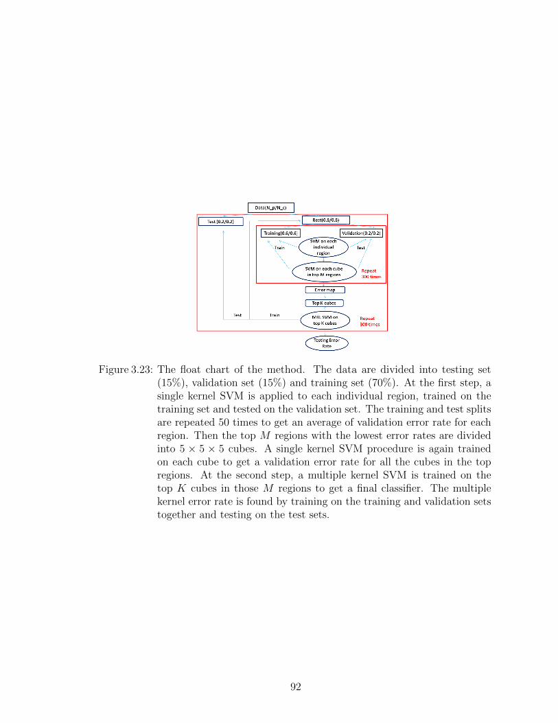
Figure 3.23: The float chart of the method. The data are divided into testing set(15%), validation set (15%) and training set (70%). At the first step, asingle kernel SVM is applied to each individual region, trained on thetraining set and tested on the validation set. The training and test splitsare repeated 50 times to get an average of validation error rate for eachregion. Then the top M regions with the lowest error rates are dividedinto 5 × 5 × 5 cubes. A single kernel SVM procedure is again trainedon each cube to get a validation error rate for all the cubes in the topregions. At the second step, a multiple kernel SVM is trained on thetop K cubes in those M regions to get a final classifier. The multiplekernel error rate is found by training on the training and validation setstogether and testing on the test sets.
92

3.5.3 Results
In this section, we presents the results of the two-step procedure to the four
data sets. We examined the performance of multiple kernel classifier mostly on two
aspects, the misclassification error rate and the identified significant regions. We
further improve the classifier by considering different challenges of the problems, such
as feature selection, kernel selection and tuning parameter selection.
Regions
At the first step, each scan was first divided into functional regions according to
MNI brain atlas (Tzourio-Mazoyer et al., 2002). Then a single linear kernel SVM was
trained on each regions. The result is a region error map with an error rate for each
region. Figure 3.24 shows the region error map for SLE data.
Figure 3.24: Individual region error map of SLE data. The three figures are 2-dimensional cross-sections through a voxel in the brain labeled by across in the figures. From left to right are the sagittal view, the coronalview and the axial view separately. The color represents the misclassifi-cation error rate on the validation set. The region with the darkest colorand point by the cross is the left thalamus.
From Figure 3.24, we can see most regions have classification error rates around
0.5. Only a few regions show error rates significant lower than random guess. Left
thalamus shows a lower error rate of 0.2851. It is observed that significantly smaller
thalamic volumes happened in SLE patients when compared to healthy controls (Ap-
penzeller et al., 2009). Left supplementary motor area also has a lower error rate
93

of 0.2973 and it is shown to be related to the pain caused by the SLE disease.
Parahippocampal and precuneus regions also show lower-than-average classification
error rates comparing to other regions in the brain. Both regions have been reported
in the diagnosis of SLE literature. Parahippocampal regions are found significant in
SLE in the work by (Cagnoli et al., 2012) and precuneus regions are related to the
memory impairment of the SLE patients (Oh et al., 2011).
Figure 3.25: Individual region error map of AD data. The three figures are 2-dimensional cross-sections through a voxel in the brain labeled by a crossin the figures. From left to right are the sagittal view, the coronal viewand the axial view separately. The color represents the misclassificationerror rate on the validation set. The region labeled by the cross in thefigures is the hippocampal regions. The region with the darkest colorunder hippocampal in the first figure is the parahippocampal region.
Figure 3.25 applied the same procedure to the AD data, showing the importance
of each region. For AD, the regions achieving the lowest error rates are left and right
parahippocampal with error rates of 0.2381 and 0.2752. Several studies report the
difference in parahippocampal regions between two groups (Van Hoesen et al., 2000).
And the left and right hippocampal regions also have error rates around 0.3. Change
in hippocampal’s volume is also reported to be a sensitive marker for pathological
AD stage (Gosche et al., 2002).
Figure 3.26 shows the region error map for MCI. For MCI data, some significant
regions are the same as in the AD case, such as parahippocampal regions and hip-
pocampal regions. But the regions’ individual error rates are higher than the ones
in AD, with error rates around 0.35. The right amygdala region shows a lower-than-
94

Figure 3.26: Individual region error map of MCI data. The three figures are 2-dimensional cross-sections through a voxel in the brain labeled by across in the figures. From left to right are the sagittal view, the coronalview and the axial view separately. The color represents the misclassifi-cation error rate on the validation set. The region labeled by the crossis the parahippocampal region.
average classification rate which was observed in other study (Pennanen et al., 2005).
Figure 3.27: Individual region error rate map of CPP. The three figures are 2-dimensional cross-sections through a voxel in the brain labeled by across in the figures. From left to right are the sagittal view, the coronalview and the axial view separately. The color represents the misclassifi-cation error rate on the validation set. The region labeled by the crossis the left thalamus.
Figure 3.27 shows the regions error rate map for CPP using linear kernel SVM.
For CPP, the region achieving the lowest error rate is cerebellum region with an error
rate of 0.2808. There are several works suggesting the connection between cerebellum
and pain perception (Moulton et al., 2010). Both left and right thalamus regions have
error rates around 0.3. It is long known that the thalamus regions are part of the pain
matrix. These regions are also found to be related to CPP in other works (As-Sanie
et al., 2012).
95

Cubes
The region unit in the above analysis is usually a complicated structure with many
small functional areas. In this step, we segmented the regions further into smaller
cubes to identify finer areas that were associated with the disease. For each training
and validation split, we first trained an individual SVM on each region and then chose
the top K regions with the lowest individual classification errors. Each region was
then segmented into 5 ∗ 5 ∗ 5 mm non-overlapped cubes as described in section 3.5.2
and a single kernel SVM was built on each cube to get an error rate for each cube. All
SVM classifiers were trained on the training set and tested on the validation set. The
result was an error map of individual error rates for cubes in the significant regions.
Figure 3.28 showed the individual cube error maps for four data sets. From top to
bottom are the maps of SLE, AD, MCI and CPP data sets. From those figures we
can tell that the top cubes in the significant regions are clustered together rather than
scattered across the whole brain. This shows that the region error rates are stable
across different training and validation splits. The regions with lower classification
error rates in one training and validation split are more likely to be in the top K in
another split. So these cubes are picked for individual SVM more frequently than
others.
From the cube error maps, we can see that not all the voxels in the cube have
similar classification power. For SLE data, thalamus shows up as a significant region
in different training and validation splits. Most of the cubes in the thalamus are
picked as significant cubes but their average classification error rates range from 0.25
to 0.4. This means not all the parts in thalamus play the same role. In order to
identify significant areas with better spatial resolution, it is better to use a finer
unit than the regions defined by MNI brain atlas. For thalamus in SLE data, the
cube achieving lower classification error is in pulvinar nuclei in thalamus. And for
AD and MCI patients, the most significant cubes are in parahippocampal gyrus in
96

parahippocampal region. For CPP, the cubes with the lowest classification error rates
are in putamen and thalamus.
97

Figure 3.28: Cube error maps of the top cubes for four data sets. From top to bottomare the maps of SLE, AD, MCI and CPP data sets. The three figuresare 2-dimensional cross-sections through a voxel in the brain labeled bya cross in the figures. From left to right are the sagittal view, the coronalview and the axial view separately. The figures show the top 100 cubeswith the lowest validation error rates in the top regions.
98

Classification Error Rate
After the individual cube error maps, we selected the top K cubes with the lowest
classification error rates to build the MKL SVM. Let {−→xn1,−→xn2, . . . ,−−→xnM} be the set
of vectors on the top K cubes for subject n. −→xnk represents the vector of voxels in
the k-th cube of subject n. For MKL SVM, we built a single kernel on each cubes.
The linear kernel for cube k between subject i and j was defined as:
Hk(i, j) =< −→xik,−→xjk >
Then the final multiple kernel H(i, j) =∑K
k=1 ηkHk(i, j) found the best linear combi-
nation of K kernels to maximize the optimization function (3.3). The multiple kernel
classifier was trained on the training and validation set together and tested on the
test set. The following table reports the classification error rate for four data sets
under different values of M and K. Tuning parameter C for SVM was 10.
Table 3.7 compares the results of traditional SVM method to the two-step proce-
dure. The first row in the Table 3.7 are the error rates of using single kernel SVM on
the whole brain. The rest of the results are the multiple kernel learning error rates
from the two-step procedure with M = 5. The results show that in all the four cases,
two-step procedure achieve an error rate lower than single kernel SVM. This confirms
C=10 SLE AD MCI CPPSVM 0.516 0.4002 0.4311 0.4444
M = 5 K = 10 0.3995 0.3158 0.3659 0.3735M = 5 K= 20 0.3935 0.3118 0.3700 0.3737M = 5 K = 50 0.451 0.3729 0.4293 0.4944M = 5 K = 100 0.423 0.3676 0.4322 0.4897
Table 3.7: MKL error rates of four data sets, M = 5. The first row is the result ofthe traditional SVM, treating all the voxels as a long vector. The numberof top regions to get the small cubes is M = 5. The number of top cubesin the final classifier is K = 10, 20, 50 and 100. The red color in eachcolumn highlights the lowest classification error rate for each data.
99

that the multiple kernel learning SVM can get a better performance by taking the
structural information into consideration.
Moreover, Table 3.7 shows that brain images have different classification power for
different diseases. AD is the easiest to classify with the lowest classification error rate
since it is a neurodegenerative disease which directly relates to the loss of the gray
matter in the brain. MCI is similar to AD but with weaker symptoms and signals.
So it is more difficult than AD. SLE has the highest classification error rate because
for the SLE data we had very few subjects to train the classifier. So it is very hard to
identify the true signal from the noise for such a high-dimension problem. Another
observation is that for a small number of regions (M = 5), adding more cubes in
the final multiple kernel analysis actually leads to a higher error rate. This means
different parts in the region are not the same and selecting the insignificant cubes in
the significant regions won’t improve the classifier.
We then compare the cases of M = 10 and K = 10, 20, 50, 100 to the classifier
of a single cube. Table 3.8 shows the MKL error rate for M = 10 for four data
sets. The first row is the error rate corresponding to M = 1 and K = 1 which
means at each test split, only the cube with the lowest validation error rate is used
for the classifier. Multiple kernel learning achieves a lower classification error than
single kernel classifier for all the four data sets and all the values of M . This shows
combining informative cubes together can give a more informative classifier.
100

C=10 SLE AD MCI CPP
M = 1 K = 1 0.4138 0.3577 0.3982 0.4522M = 10 K = 10 0.3885 0.318 0.3664 0.3633M = 10 K = 20 0.3875 0.3150 0.3779 0.3622M = 10 K = 50 0.3575 0.3226 0.3797 0.3764M = 10 K = 100 0.3482 0.3325 0.3722 0.3811
Table 3.8: MKL error rates of four data sets, M = 10. The number of top regionsto get the small cubes is M = 10. The number of top cubes in the finalclassifier is K = 10, 20, 50 and 100. The red color in each column highlightsthe lowest classification error rate for each data. The first row is the testerror for single kernel SVM on the top cube with the lowest validationerror.
Dimension Reduction
Selecting top cubes from all the regions in the brain didn’t give a good classifier.
This was because of the high dimensionality of the brain image data and the small
sample size of the problem. The signals were weak comparing to noise and only in
few voxels. So it was very hard to pick up the signals from the whole brain using
only few training subjects. In order to solve this problem, we tried two different
approaches here to reduce the dimensionality of the problem. One was to do feature
selection. Instead of using the original signals, we used a vector as a very coarse
estimation of the density function of each cube. The kernel took the estimates of the
density function not the voxels values. So this method extracted new features from
the original data to reduce the dimension. Another solution was to start from a few
informative regions rather than all the regions in the brain. This method reduced the
dimension by borrowing extra information from expert knowledge. In this study, we
chose six informative regions for different disease according to the literature about
the disease.
Feature Selection For the feature selection method, we used an equally spaced
10-bin histogram to represent each cube. The features for the cube k was a vector
101

−→z = {z1, z2, . . . , z10}, with∑10
i=1 zi = 1. Since all the values were normalized between
0 and 1, zi was the proportion of voxels with signal values between 0.1 ∗ (i− 1) and
0.1 ∗ i. Then the kernels were built on −→z rather than original signal −→x .
Figure 3.29: Cube error maps of three data sets, using density feature. From thetop to the bottom are SLE, AD and MCI separately. First, each regionis represented by a 10-bin histogram of all its voxels and then a singlekernel SVM is trained on each region. Top M regions are selected tofurther break down into small 5× 5× 5 cubes. Then each cube is againrepresented by a 10-bin histogram of its voxels and an SVM is trainedon each cube. The figure presents the classification error rate of the top100 cubes with the lowest error rates.
We repeated the two-step procedure taking density estimates as features instead
of original signal to produce another cube error map. Figure 3.29 shows the cube
error maps for the three data sets using density features. From the top to the bottom
are SLE, MCI and AD datasets. Comparing Figure 3.29 to 3.28, we can see there
102

are some cubes showing significant in both Figures. Figure 3.29 also confirms the
thalamus regions for SLE data and parahippocampal regions for AD and MCI data
sets. It also reports some regions that are not identified by the classifier taking original
signals, such as the temporal regions in the SLE data. The selected cubes are more
scattered across the whole brain rather than concentrated in few regions as Figure
3.28.
After getting the top cubes, we trained a MKL on the top cubes, taking only the
density estimates. Table 3.9 shows the multiple kernel classification error for three
data sets using density as features. Comparing to Table 3.7, density features doesn’t
achieve a better classifier. For SLE data, the best error rate is around 0.38 while
using the original signal the error rate is around 0.34. For AD data, the best error
rate is around 0.35 for density features and the best error rate is around 0.31 for
signal features. For MCI, the error rate is higher than AD data, with a value around
0.38 for density features and a value around 0.36 for using original signal. This may
suggest that a 10-bin vector can not represent the density function of each kernel
well. AD is still the one with the lowest classification error rates and SLE data was
the one with the highest error rates.
103

Density Feature Original SignalC=10 SLE AD MCI SLE AD MCI
M=10 K=10 0.4455 0.3605 0.4038 0.3885 0.318 0.3664M=10 K=20 0.4317 0.3658 0.3936 0.3875 0.3150 0.3779M=10 K=50 0.4307 0.3599 0.3831 0.3575 0.3226 0.3797M=10 K=100 0.411 0.3692 0.3787 0.3482 0.3325 0.3722
Table 3.9: Multiple kernel classification error rates of three data sets, using densityfeatures. Each region was first represented by a 10-bin histogram andthen trained an SVM classifier to get a validation error rate map of theregions. The top regions with the lowest error rates were broken downinto small cubes. Then each cube was represented by a 10-bin histogramto train a single kernel SVM to get validation error map for the cubes.The MKL SVM takes the 10-bins histogram of the top cubes to train aclassifier. The tables shows the classification error rate for both densityfeatures and original signals. The red color highlights the lowest error rateof each column.
Region Selection In this part, we focused our analysis on a few regions instead
of the whole brain. We choose six informative regions for each disease according to
the extra knowledge about the disease. The regions selected for SLE is left and right
thalamus ares, left and right supplementary motor areas and left and right precuneus
areas. The regions selected for AD is left and right parahippocampal areas, left and
right lingual areas and left and right precuneus areas. The regions selected for MCI are
left and right parahippocampal areas, left and right hippocampus areas and left and
right precuneus areas. The regions are selected before the analysis. We first applied
a single kernel SVM on each of the six informative regions to get a classification
error for each region. Figure 3.30 shows the region error rate map for informative
individual region using linear kernel. From Figure 3.30, we can see not all the pre-
selected regions have small classification error rates. The thalamus regions in the SLE
and the parahippocampal regions in AD and MCI have relative small classification
error rates.
We then selected the top three regions with the lowest classification error rates for
each training and test split and divided the selected region into small 5 ∗ 5 ∗ 5 cubes.
104
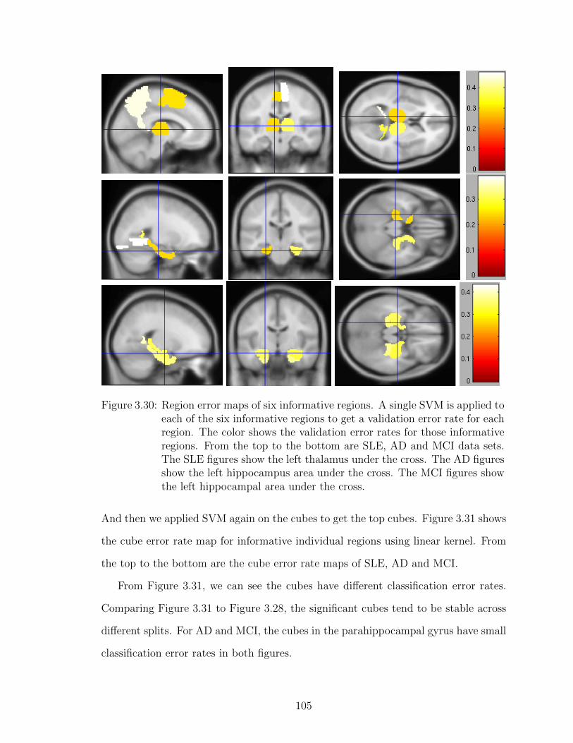
Figure 3.30: Region error maps of six informative regions. A single SVM is applied toeach of the six informative regions to get a validation error rate for eachregion. The color shows the validation error rates for those informativeregions. From the top to the bottom are SLE, AD and MCI data sets.The SLE figures show the left thalamus under the cross. The AD figuresshow the left hippocampus area under the cross. The MCI figures showthe left hippocampal area under the cross.
And then we applied SVM again on the cubes to get the top cubes. Figure 3.31 shows
the cube error rate map for informative individual regions using linear kernel. From
the top to the bottom are the cube error rate maps of SLE, AD and MCI.
From Figure 3.31, we can see the cubes have different classification error rates.
Comparing Figure 3.31 to Figure 3.28, the significant cubes tend to be stable across
different splits. For AD and MCI, the cubes in the parahippocampal gyrus have small
classification error rates in both figures.
105

Figure 3.31: Cube error maps of cubes in informative regions. A single SVM is appliedto all the cubes in the top three regions with the lowest validation errorrates. The figure shows the validation error rates for those cubes. Fromthe top to the bottom are SLE, AD and MCI data sets.
After getting the cube error rate maps, we applied a multiple kernel analysis on
the top cubes. Table 3.10 shows the multiple kernel error rates for three data sets.
We compare the classification error rate of applying the two-step procedure on only
the informative regions to the method starting from all the regions. Table 3.10 shows
that using a few selected information regions can improve the performance of the
classifier. The classification error rate is around 0.37 for SLE data when using all
the regions in the brain scan with M = 20 and K = 50. But the rate is only 0.32
when using only the informative regions for K = 50. And for AD, the error rates are
around 0.31 when using all the regions and decrease to 0.30 for K = 20. For MCI,
106

C = 10 Informative All RegionsM 3 20
SLEK = 20 0.32375 0.3932K = 50 0.31925 0.3762
ADK = 20 0.2991 0.3132K = 50 0.3234 0.3116
MCIK = 20 0.34007 0.3849K = 50 0.34436 0.3840
Table 3.10: MKL error rates of on informative regions. We applied the two-stepprocedure on six informative regions that are selected according to theextra knowledge about the disease. At the first step, A single kernel SVMis applied to the regions and then three regions with the lowest error ratesare broken down into smaller cubes. Then a single kernel SVM is appliedto all the cubes in the selected regions. The final classifier is built on Kcubes with the lowest error rates. We compare the method of using onlythe informative regions with the method starting from the whole brain.
the previous error rates were around 0.38 for all the regions and were around 0.34 for
informative regions. This shows that focusing on the informative regions can reduce
the dimension, making the classification an easier task.
Kernel Selection
For the same features, we can also design different kernels to find the best classifier.
Linear kernel is the simplest one of which the feature space is just the original signal.
And the final classifier is a hyperplane in the original spaces. In this study, we also
tried the Gaussian kernel which produced more complex features than the linear
kernel and could fit any boundaries. The Gaussian kernel taking two vectors −→xi and
−→xj is defined as:
H(−→xi ,−→xj) = exp{||−→xi −−→xi ||2
Cgauss}
The complexity of the kernel is controlled by parameter Cgauss. The smaller the Cgauss
gets, the more complex the classifier is. We used cross-validation to find the tuning
parameter Cgauss for Cgauss = 1, 10 and 50. We applied the same procedure to the
107
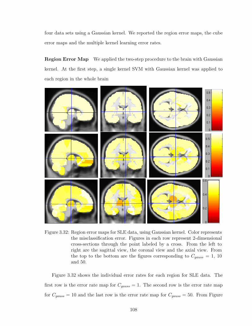
four data sets using a Gaussian kernel. We reported the region error maps, the cube
error maps and the multiple kernel learning error rates.
Region Error Map We applied the two-step procedure to the brain with Gaussian
kernel. At the first step, a single kernel SVM with Gaussian kernel was applied to
each region in the whole brain
Figure 3.32: Region error maps for SLE data, using Gaussian kernel. Color representsthe misclassification error. Figures in each row represent 2-dimensionalcross-sections through the point labeled by a cross. From the left toright are the sagittal view, the coronal view and the axial view. Fromthe top to the bottom are the figures corresponding to Cgauss = 1, 10and 50.
Figure 3.32 shows the individual error rates for each region for SLE data. The
first row is the error rate map for Cgauss = 1. The second row is the error rate map
for Cgauss = 10 and the last row is the error rate map for Cgauss = 50. From Figure
108

3.32, we can see that when Cgauss = 1, the classifier is too simple to separate the
two groups. So all the regions have similar error rate, close to 0.5. As Cgauss goes
up, the classifier becomes more complex and able to distinguish the patients from
the healthy controls. When Cgauss = 50, the Gaussian kernel can tell the informative
regions from the non-informative one. Thalamus regions show a better classification
error than other regions in the classifiers using Cgauss = 50.
Cube Error Map After getting the top regions, we also tested the Gaussian kernel
on individual cubes. For each split, we selected the top M regions and divided each
region into 5 ∗ 5 ∗ 5 cubes. A single SVM with Gaussian kernel was applied to each
individual cube. And the cube error rate maps plot the top cubes with their error
rates.
Figure 3.33 shows the cube error rate maps for SLE data set using Gaussian
kernels for different Cgauss values. From the top to the bottom are the Gaussian
kernels with Cgauss = 1, Cgauss = 10 and Cgauss = 50. All three figures have similar
patterns across different values of Cgauss. They all identify the cubes in the thalamus
and the somatosensory cortex. For larger values of Cgauss, the informative cubes are
more clustered together.
109

Figure 3.33: Cube error maps for SLE data, using Gaussian kernel. Color representsthe misclassification error. Figures in each row represent 2-dimensionalcross-sections through the point labeled by a cross. From the left toright are the sagittal view, the coronal view and the axial view. Fromthe top to the bottom are the figures corresponding to Cgauss = 1, 10and 50.
Multiple Kernel Error
After getting a cube error rate map, we selected the top regions to build the final
classifier. Multiple kernel error rates were found by applying a single Gaussian kernel
on top cubes and then combining them in the multiple kernel step. The classifier
was trained on the training set and validation set together and tested on the testing
set. We compared the multiple kernel error rates of Gaussian kernel with the linear
kernel. We presented the results for different tuning parameters C and Cgauss.
Table 3.11 shows the multiple kernel learning results for all four data sets, compar-
110

C = 10 Gaussian LinearCgauss 1 10 50 NA
SLE
M = 5 K = 20 0.476 0.501 0.488 0.393M = 5 K = 50 0.459 0.482 0.475 0.451M = 10 K = 20 0.485 0.481 0.466 0.387M = 10 K = 50 0.468 0.475 0.467 0.357
AD
M = 5 K = 20 0.316 0.359 0.329 0.311M = 5 K = 50 0.319 0.336 0.312 0.372M = 10 K = 20 0.280 0.330 0.318 0.315M = 10 K = 50 0.285 0.325 0.322 0.322
MCI
M = 5 K = 20 0.335 0.367 0.380 0.370M = 5 K = 50 0.307 0.353 0.366 0.429M = 10 K = 20 0.330 0.365 0.374 0.377M = 10 K = 50 0.314 0.362 0.377 0.379
CPP
M = 5 K = 20 0.422 0.477 0.470 0.373M = 5 K = 50 0.405 0.477 0.479 0.494M = 10 K = 20 0.400 0.48 0.479 0.362M = 10 K = 50 0.397 0.488 0.484 0.376
Table 3.11: Multiple kernel learning error rates of four data sets, using Gaussian ker-nel. We applied the two-step procedure to the whole brain with Gaussiankernel and compare the results to the results of linear kernel. We trieddifferent number of regions and cubes for the classifier, M = 5 and 10,K = 20 and 50.
ing the results between Gaussian kernel and linear kernel. We tried four combinations,
with M = 5, 10 and K = 20, 50. In SLE and CPP cases, the linear kernel perfor-
mances better than the Gaussian kernel. The best error rate of SLE was 0.357 for
linear kernel with M = 10 and K = 50. For the same M and K, the best error rate
of SLE for Gaussian kernel is 0.467 under Cgauss = 50. And for CPP, the linear kernel
can achieve an error rate of 0.362 with M = 10 and K = 20. Gaussian kernel gets
0.4 for the same K and M . Since for both SLE and CPP data, we only have a small
sample size, about 40 subjects in both data sets, so a simple classifier performs better
than a complex one.
111

For AD and MCI data sets, the Gaussian kernel performs better than linear kernel.
The best error rate of AD for Gaussian kernel is 0.28 for M = 10 and K = 10 and the
linear kernel gets 0.315 for the same M and K. The best error rate of MCI is 0.307
and the best error rate for linear kernel is 0.37. Because for AD and MCI data sets,
we have much more subjects than in SLE and CPP studies, so the data can support
a more complex classifier than the linear classifier.
In the linear kernel case, if the M = 5, then including more cubes will not enhance
the performance of the classifier. For M = 10, including 20 or 50 cubes give similar
classification error rate. This is not the case in the linear kernel. For Gaussian kernel,
including more cubes will not increase the error rates. So Gaussian kernel can combine
more kernels together, supporting a more complicated classifier.
For the individual region error map, Cgauss = 1 produces a classifier which overfits
the data. But in the MKL case, Cgauss = 1 generally gets better results than Cgauss =
10 and 50. In the MKL cases, we have more information of the class which can be
used to fit a more complicated classifier.
3.6 Discussion
This chapter covers the analysis of structural MRI. VBM and SVM are the most
popular methods in the structural MRI analysis. VBM is a voxel-based method
which takes one voxel at a time and ignores the interaction between the voxels. SVM
is a multivariate method which aligns all the voxels as a long vector and ignores the
physical location of each voxel.
We propose a two-step procedure, taking both the interaction and the location
information into consideration. The new method uses the multiple kernel learning
technique which builds sub-kernels on different variables and then combines them in
the second step. In our two-step procedure, we first select the informative regions
based on the single kernel SVM analysis and then train a multiple kernel SVM to
112
combine the informative regions.
We test the performance of the two-step procedure in a simulation study. The
study shows that the performance of the multiple kernel classifier is related to several
factors, such as the strength of the signal, the level of the spatial correlation in the
data and the number of kernels taken by the multiple kernel classifier.
In the real data analysis, we compare the two-step procedure to the traditional
single kernel SVM in four data sets. The two-step procedure can achieve a lower
classification error rate in all four cases. This suggests that using the multiple kernel
SVM to allow a more flexible classifier can improve the performance.
We also test our method on few informative regions that are selected according to
extra knowledge about the disease. Starting from few informative regions can reduce
the misclassification error. Moreover we compare the results of the Gaussian kernel
and the linear kernel. The linear kernel performs better in the cases with small sample
size. As the sample size goes up, the data can support more complicated classifier.
113

CHAPTER IV
Conclusion and Future Work
114

This thesis discusses both the fMRI analysis and the structural MRI analysis.
The former is a signal decomposition problem, decomposing the observed signals
into different sources to identify the regions activated by the stimuli. The latter is
a classification problem, classifying the subjects into the patients and the healthy
controls to detect the regions affected by a disease. We propose new methods for
both analyses and compare the results to the existing methods. We also discusses
some possible directions for the future works.
4.1 fMRI Analysis
Chapter II covers the fMRI analysis. The fMRI signal is a series of brain scans
recording the neural activities evoked by some stimuli. The purpose of the fMRI
analysis is to identify the regions that respond to the stimuli. One challenge of the
fMRI analysis is the high temporal and spatial correlation in the data. One popular
method, GLM, uses an autoregressive model to model the temporal correlation. The
autoregressive model assumes the same level of temporal correlation across the whole
brain which is not a valid assumption. Instead of assuming a uniform correlation,
we propose a Gaussian process model that allows different levels of correlation for
different voxels. In the Gaussian process model, the observed signal is divided into
three deterministic parts: a constant representing the scale of the time series, a linear
function representing a linear trend usually observed in fMRI signals and a stimuli-
related part measuring the strength of the neural activity and two random processes:
a Gaussian process with Gaussian kernel measuring the temporal correlation of the
signal and a white noise.
The estimation can either use a Bayesian approach, imposing a prior distribution
on the parameters or use a frequentist approach through the EM algorithm. The
simulation study shows that we can obtain reasonable estimates of the parameters
using both methods. The real data analysis shows that different voxels in the brain
115

have different levels of temporal correlation. The correlation level is a smooth function
across the whole brain. The activation areas identified by the new method is similar
to the GLM method but with smoother boundaries.
Future Work
Gaussian process approach is a voxel-based method which means it analyzes one
voxel at a time, ignoring the spatial correlation between the voxels. In future works,
we can incorporate the spatial information into the covariance matrix of the Gaussian
process. This means that the neighboring voxels are not modeled independently
anymore. For the signal of voxel vi at time ts and the signal of voxel vj at time tk,
the correlation is
Cor(X{vi,ts}, X{vj ,tk}) = f(vi − vj, ts − tk),
where f(τ, ν) is a decreasing function in both τ and ν. In this case, we not only
capture the temporal correlation but also model the spatial correlation of the fMRI
signals.
GLM and ICA are two widely used methods for fMRI analysis. The popularity of
GLM comes from its easy estimation and simple interpretation. The model specifies
each component and estimates the parameters in explicit forms. However, GLM is
a voxel-based method which does not take the spatial correlation into consideration.
ICA is a multivariate methods which analyzes the whole brain together instead of
one voxel at a time. However, ICA is an unsupervised method, with difficulties in the
interpretation of those independent components.
We desire a multivariate supervised learning method that have the advantages
from both GLM and ICA . Chapter II provides one possible solution, using a Gaussian
process methods, dividing the signals into the deterministic experiment-related part
116

and the random Gaussian process part. The experiment-related part captures the
signals of the neural activity and the Gaussian process models the temporal and
spatial correlation in the fMRI scans. So designing a covariance matrix that can
reflect both the temporal and spatial information is the key for the Gaussian process
model.
4.2 Structural MRI Analysis
Chapter III covers the structural MRI analysis. The structural image is one scan
of the whole brain with superb spatial resolution. It provides a detailed map of
the brain, capturing the subtle changes brought by any effects such as diseases. The
purpose of the structural MRI analysis is to classify the subjects into the patients and
the healthy control group and to identify the regions that are affected by the diseases.
One existing method, based on the machine learning technique SVM, treats all the
voxels in the brain as a long vector. It ignores the local structures of the functional
regions and the spatial correlation among the neighboring voxels. We propose a
two-step procedure which takes the regional structure into consideration through the
multiple kernel learning technique. The multiple kernel learning combines different
kernels from different sources, allowing different variables contributing in different
ways.
In the structural MRI analysis, we design the individual kernels on small regions
in the brain. At the first step, the whole brain is divided into functional regions
according to the AAL atlas of the human brain (Fischl et al., 2002). A single kernel
SVM classifier is trained on each region to measure the importance of each region.
Then the top M regions with the lowest classification error rates are selected and
further broken down into small 5 × 5 × 5 cubes. A single kernel SVM is applied to
the individual cubes to select the top K cubes with the lowest classification error
rates. At the second step, the multiple kernel SVM builds a kernel on each cube first
117

and then combine them together. In this segmentation and combination steps, the
multiple kernel learning achieves a more flexible classifier than the traditional SVM
method.
Applying the two-step procedure on the four data sets shows that the new method
can achieve a classifier better than the traditional SVM. For all the four data sets, the
two-step procedure gets a lower error rate than using only the single kernel. Moreover,
it can identify the disease-related regions that are confirmed by other works.
Future Work
For all the four data sets, both the traditional SVM and the multiple kernel SVM
can not achieve a classification error rate good enough for the clinical diagnosis. One
possible explanation lies in the preprocessing steps. The registration step maps all
the brain scans into the same template, reducing the group differences between the
patients and the healthy controls. In the future work, we can test the method on the
unprocessed data.
In our real data analysis, we compare the performances between Gaussian kernel
and the linear kernel. The results show that for small data set, about 40 subjects,
the linear kernel can outperform Gaussian kernel. But for data set with 100 subjects,
Gaussian kernel achieves a lower classification error rate than the linear kernel. The
relation between the performance of different types of kernels and the sample size
need further investigation.
In our method, we choose to select the informative region first and then select the
informative cubes within the informative regions. We use the cubes of size 5× 5× 5
as the smallest unit that our method can detect. There is a trade off between the size
of the unit and the stability of the method. For small unit, such as the individual
voxel, the method can identify very small area but with a lot of false positive voxels.
For large unit, such as using the AAL regions to train the SVM, the method can
118

get stable results but very coarse resolution. The size of the unit for multiple kernel
method also is a direction of further research.
119

BIBLIOGRAPHY
120

BIBLIOGRAPHY
ACOG Committee on Practice Bulletins–Gynecology. (2004), Acog practice bulletinno. 51. chronic pelvic pain., Obstet Gynecol., 103 (3), 589–605.
Aguirre, G. K., E. Zarahn, and M. D’Esposito (1998), The variability of human, boldhemodynamic responses, NeuroImage, 8 (4), 360–369.
Appenzeller, S., B. Pike, L. Rittner, G. Leonard, M. Veilleux, and A. E. Clarke (2009),Thalamic volumes predict cognitive impairment evaluated by speed processing tasksin systemic lupus erythematosus [abstract], in Arthritis Rheum 2009, vol. 60 Suppl.
As-Sanie, S., R. Harris, V. Napadow, J. Kim, G. Neshewat, A. Kairys, D. Williams,D. Clauw, and T. Schmidt-Wilcke (2012), Changes in regional gray matter volumein women with chronic pelvic pain: a voxel-based morphometry study., Pain.,153 (5), 1006–14.
Ashburner, J., and K. Friston (1999), Nonlinear spatial normalization using basisfunctions, Human Brain Mapping, 7 (4), 254–266.
Ashburner, J., and K. Friston (2005), Unified segmentation, NeuroImage, 26, 839–851.
Ashburner, J., and K. J. Friston (2000), Voxel-based morphometrythe methods, Neu-roimage, 11, 805–821.
Ashburner, J., P. Neelin, D. L. Collins, A. C. Evans, and K. Friston (1997), Incorpo-rating prior knowledge into image registration, NeuroImage, 6, 344–352.
Asllani, I., C. Habeck, N. Scarmeas, A. Borogovac, T. R. Brown, and Y. Stern (2007),Multivariate and univariate analysis of continuous arterial spin labeling perfusionMRI in Alzheimer’s disease, J Cereb Blood Flow Metab, 28 (4), 725–736.
Bell, A. J., and T. J. Sejnowski (1995), An information-maximisation approach toblind separation and blind deconvolution, Neural Computation, 7, 1129–1159.
Benjamini, Y., and Y. Hochberg (1995), Controlling the false discovery rate: A prac-tical and powerful approach to multiple testing, Journal of the Royal StatisticalSociety. Series B (Methodological), 57 (1), 289–300.
121

Biswal, B. B., and J. L. Ulmer (1999), Blind source separation of multiple signalsources of fmri data sets using independent component analysis., Journal of com-puter assisted tomography, 23 (2), 265–271.
Bottino, C. M., C. C. Castro, R. Gomes, C. Buchpiguel, R. Marchetti, and M. Neto(2002), Volumetric mri measurements can differentiate alzheimer’s disease, mildcognitive impairment, and normal aging., Int Psychogeriatr., 14 (1), 59–72.
Boynton, G. M., S. A. Engel, G. H. Glover, and D. J. Heeger (1996), Linear systemsanalysis of functional magnetic resonance imaging in human v1, The Journal ofNeuroscience, 16, 4207–4221.
Cagnoli, P., P. Sundgren, A. Kairys, C. Graft, D. Clauw, S. Gebarski, W. McCune,and T. Schmidt-Wilcke (2012), Changes in regional brain morphology in neuropsy-chiatric systemic lupus erythematosus., J Rheumatol., 39 (5), 959–67.
Calhoun, V., T. Adali, G. Pearlson, and J. Pekar (2001), Spatial and temporal inde-pendent component analysis of functional mri data containing a pair of task-relatedwaveforms, Human Brain Mapping, 13 (1), 43–53.
Calhoun, V. D., T. Adali, L. K. Hansen, J. Larsen, and J. J. Pekar (2003), Ica offunctional mri data: An overview, in in Proceedings of the International Workshopon Independent Component Analysis and Blind Signal Separation, pp. 281–288.
Cardoso, J.-F. (1997), Infomax and maximum likelihood for blind source separation,Signal Processing Letters, IEEE, 4 (4), 112–114.
Cardoso, J.-F., and A. Souloumiac (1993), Blind beamforming for non gaussian sig-nals, IEE Proceedings-F, 140, 362–370.
Chan, D., et al. (2001), Patterns of temporal lobe atrophy in semantic dementia andAlzheimer’s disease., Annals of neurology, 49 (4), 433–442.
Comon, P. (1994), Independent component analysis, a new concept?, Signal Process-ing, 36 (3), 287–314.
Cox, D. D., and R. Savoy (2003), fMRI ’Brain Reading’: detecting and classifyingdistributed patterns of fMRI activity in human visual cortex, NeuroImage, 19 (2),261–270.
Davatzikos, C. (2004), Why voxel-based morphometric analysis should be used withgreat caution when characterizing group differences, Neuroimage, 23 (1), 17–20.
Davis, R. (2001), Encyclopedia of Environmetrics, chap. Section on Stochastic Mod-eling and Environmental Change, Wiley.
Delfosse, N., and P. Loubaton (1995), Adaptive blind separation of independentsources: A deflation approach, Signal Processing, 45 (1), 59 – 83.
122

Draganski, B., C. Gaser, V. Busch, G. Schuierer, U. Bogdahn, and A. May (2004),Neuroplasticity: changes in grey matter induced by training., Nature, 427 (6972),311–312.
Fan, Y., D. Shen, and C. Davatzikos (2005), Classification of structural images viahigh-dimensional image warping, robust feature extraction, and svm, in Proceedingsof the 8th international conference on Medical Image Computing and Computer-Assisted Intervention - Volume Part I, MICCAI’05, pp. 1–8, Springer-Verlag.
Fan, Y., et al. (2007), Multivariate examination of brain abnormality using bothstructural and functional mri., NeuroImage, 36 (4), 1189–99.
Fischl, B., et al. (2002), Neuron, 33 (3), 341–355.
Friston, K., J. Ashburner, C. Frith, J. Poline, J. D. Heather, and R. Frackowiak(1995a), Spatial registration and normalization of images, Human Brain Mapping,2, 165–189.
Friston, K., A. Holmes, K. Worsley, J. Poline, C. Frith, and R. Frackowiak (1995b),Statistical parametric maps in functional imaging: A general linear approach, Hu-man Brain Mapping, 2, 189–210.
Friston, K., S. Williams, R. Howard, R. Frackowiak, and R. Turner (1996a),Movement-related effects in fMRI time-series, Magnetic Resonance in Medicine,35, 346–355.
Friston, K., J. Ashburner, S. Kiebel, T. Nichols, and W. Penny (Eds.) (2007), Sta-tistical Parametric Mapping: The Analysis of Functional Brain Images, AcademicPress.
Friston, K. J., S. Williams, R. Howard, R. S. Frackowiak, and R. Turner (1996b),Movement-related effects in fMRI time-series., Magnetic resonance in medicine,35 (3), 346–355.
Genovese, C. R., N. A. Lazar, and T. Nichols (2002), Thresholding of statistical mapsin functional neuroimaging using the false discovery rate, NeuroImage, 15 (4), 870– 878.
Gitelman, D. R., J. Ashburner, K. J. Friston, L. K. Tyler, and C. J. Price (2001),Voxel-based morphometry of herpes simplex encephalitis., NeuroImage, 13, 623–631.
Gonen, M., and E. Alpaydin (2011), Multiple kernel learning algorithms, J. Mach.Learn. Res., 12, 2211–2268.
Gosche, K. M., J. A. Mortimer, C. D. Smith, W. R. Markesbery, and D. A. Snowdon(2002), Hippocampal volume as an index of Alzheimer neuropathology, Neurology,58 (10), 1476–1482.
123

Greenstein, D., B. Weisinger, J. D. Malley, L. Clasen, and N. Gogtay (2012), Usingmultivariate machine learning methods and structural mri to classify childhoodonset schizophrenia and healthy controls, Frontiers in Psychiatry, 3.
Huettel, S. A., A. W. Song, and G. McCarthy (2009), Functional Magnetic ResonanceImaging, Second Edition, Massachusetts: Sinauer.
Hyvarinen, A. (1998), New approximations of differential entropy for independentcomponent analysis and projection pursuit, in NIPS ’97: Proceedings of the 1997conference on Advances in neural information processing systems 10, pp. 273–279,MIT Press.
Hyvarinen, A. (1999), Survey on independent component analysis, Neural ComputingSurveys, 2, 94–128.
Hyvarinen, A., and E. Oja (2000), Independent component analysis: algorithms andapplications, Neural Networks, 13 (4-5), 411–430.
Jones, M. C., and R. Sibson (1987), What is projection pursuit?, Journal of the RoyalStatistical Society. Series A (General), 150 (1), 1–37.
Josephs, O., and R. N. A. Henson (1999), Event-related functional magnetic reso-nance: modelling, inference and optimization, Phil. Trans. R. Soc. Lond. B, 354,1215–1228.
Josephs, O., R. Turner, and K. Friston (1997), Event-related fmri, Human BrainMapping, 5 (4), 243–248.
Karas, G., et al. (2003), A comprehensive study of gray matter loss in patients withalzheimer’s disease using optimized voxel-based morphometry., NeuroImage, 18 (4),896–907.
Kawasaki, Y., et al. (2007), Multivariate voxel-based morphometry successfully differ-entiates schizophrenia patients from healthy controls, NeuroImage, 34 (1), 235–242.
Keller, S. S., and N. Roberts (2009), Measurement of brain volume using mri: soft-ware, techniques, choices and prerequisite, Journal of Anthropological Science, 97,127–151.
Kinser, P. A., and P. Grobstein (2000), Brain structures and their funcitions.
Kloppel, S., et al. (2008), Automatic classification of MR scans in Alzheimer’s disease,Brain, 131 (3), 681–689.
Kopelman, M., et al. (2001), Structural mri volumetric analysis in patients withorganic amnesia, 2: correlations with anterograde memory and executive tests in40 patients, J Neurol Neurosurg Psychiatry., 71 (1), 23–28.
124

Kubicki, M., M. Shenton, D. Salisbury, Y. Hirayasu, K. Kasai, R. Kikinis, F. Jolesz,and R. McCarley (2002), Voxel-based morphometric analysis of gray matter in firstepisode schizophrenia., NeuroImage, 17 (4), 1711–9.
LaConte, S., S. Strother, V. Cherkassky, J. Anderson, and X. Hu (2005), Supportvector machines for temporal classification of block design fMRI data, Neuroimage,26, 317–329.
Lanckriet, G. R. G., N. Cristianini, P. Bartlett, L. E. Ghaoui, and M. I. Jordan (2004),Learning the kernel matrix with semidefinite programming, J. Mach. Learn. Res.,5, 27–72.
Lao, Z., D. Shen, Z. Xue, B. Karacali, S. M. Resnick, and C. Davatzikos (2004),Morphological classification of brains via high-dimensional shape transformationsand machine learning methods., Neuroimage, 21 (1), 46–57.
Lyoo, I., M. Kim, A. Stoll, C. Demopulos, A. Parow, S. Dager, S. Friedman, D. Dun-ner, and P. Renshaw (2004), Frontal lobe gray matter density decreases in bipolari disorder, Biol Psychiatry, 15 (55), 648–51.
Magnin, B., L. Mesrob, S. Kinkingnhun, M. Plgrini-Issac, O. Colliot, M. Sarazin,B. Dubois, S. Lehricy, and H. Benali (2009), Support vector machine-based clas-sification of alzheimer’s disease from whole-brain anatomical mri., Neuroradiology,51 (2), 273–283.
Maguire, E. A., D. G. Gadian, I. S. Johnsrude, C. D. Good, J. Ashburner, R. S. J.Frackowiak, and C. D. Frith (2000), Navigation-related structural change in thehippocampi of taxi drivers, Proceedings of the National Academy of Sciences, 97 (8),4398–4403.
McKeown, M., L. K. Hansen, and T. J. Sejnowski (2003), Independent componentanalysis for fmri: What is signal and what is noise?, Current Opinion in Neurobi-ology, 13 (5), 620–629.
McKeown, M. J., S. Makeig, G. G. Brown, T. P. Jung, S. S. Kindermann, A. J.Bell, and T. J. Sejnowski (1998), Analysis of fmri data by blind separation intoindependent spatial components., Hum Brain Mapp, 6 (3), 160–188.
Mechelli, A., C. Price, K. Friston, and J. Ashburner (2005), Voxel-based morphometryof the human brain: Methods and applications, Current Medical Imaging Reviews,pp. 105–113.
Moulton, E. A., J. D. Schmahmann, L. Becerra, and D. Borsook (2010), The cerebel-lum and pain: Passive integrator or active participator ?, Brain Research Review,65 (1), 14–27.
Mueller, S. G., M. W. Weiner, L. J. Thal, R. C. Petersen, C. Jack, W. Jagust,J. Q. Trojanowski, A. W. Toga, and L. Beckett (2005), The alzheimer’s diseaseneuroimaging initiative., Neuroimaging clinics of North America, 15 (4), 867–77.
125

Neal, R. M. (1998), Regression and classification using Gaussian process priors (withdiscussion), Bayesian Statistics, 6, 475–501.
Noble, W. S. (2004), Support vector machine applications in computational biology,chap. 3, Computational molecular biology, MIT Press.
Ogawa, S., T.-M. Lee, A. S. Nayak, and P. Glynn (1990), Oxygenation-sensitive con-trast in magnetic resonance image of rodent brain at high magnetic fields, MagneticResonance in Medicine, 14 (1), 68–78.
Oh, D., S. Kim, S. Jung, Y. Sung, S. Bang, S. Bae, and Y. Choi (2011), Precuneushypoperfusion plays an important role in memory impairment of patients withsystemic lupus erythematosus., J Rheumatol., 20 (8), 855–60.
Pennanen, C., et al. (2005), A voxel based morphometry study on mild cognitiveimpairment, Journal of Neurology, Neurosurgery & Psychiatry, 76 (1), 11–14.
Petersen, K., L. Hansen, T. Kolenda, E. Rostrup, and S. Strother (2000), On theindependent components in functional neuroimages, in In Second InternationalSymposium on Independent Component Analysis and Blind Signal Separation, pp.615–620.
Petersen, R. C., G. E. Smith, S. C. Waring, R. J. Ivnik, E. Kokmen, and E. G.Tangelos (1997), Aging, memory, and mild cognitive impairment, InternationalPsychogeriatrics, 9 (Supplement S1), 65–69.
Pham, D. T., and P. Garat (1997), Blind separation of mixture of independent sourcesthrough a maximum likelihood approach, in In Proc. EUSIPCO, pp. 771–774.
Phillips, C. L., et al. (2011), Relevance vector machine consciousness classifier appliedto cerebral metabolism of vegetative and locked-in patients, NeuroImage, 56, 797–808.
Price, S., D. Paviour, R. Scahill, J. Stevens, M. Rossor, A. Lees, and N. Fox (2004),Voxel-based morphometry detects patterns of atrophy that help differentiate pro-gressive supranuclear palsy and parkinson’s disease., NeuroImage, 23 (2), 663–9.
Purdon, P. L., and R. M. Weisskoff (1998), Effect of temporal autocorrelation dueto physiological noise and stimulus paradigm on voxel-level false-positive rates infmri, Human Brain Mapping, 6 (4), 239–249.
Rajapakse, J. C., F. Kruggel, J. M. Maisog, and D. Y. von Cramon (1998), Modelinghemodynamic response for analysis of functional mri time-series, Human BrainMapping, 6 (4), 283–300.
Rasmussen, C. E., and C. Williams (2006), Gaussian Processes for Machine Learning,MIT Press.
126

Roy, C., and C. Sherrington (1890), On the regulation of the blood-supply of thebrain, Journal of Physiology, 11 (1-2), 85–158.17.
Salmond, C., J. Ashburner, F. Vargha-Khadem, A. Connelly, D. G. Gadian, andK. Friston (2002), The precision of anatomical normalisation in the medial temporallobe using spatial basis functions, NeuroImage, 17 (1), 507–512.
Schroeter, M. L., T. Stein, N. Maslowski, and J. Neumann (2009), Neural correlates ofalzheimer’s disease and mild cognitive impairment: A systematic and quantitativemeta-analysis involving 1351 patients, NeuroImage, 47 (4), 1196–1206.
Shenton, M. E., R. Kikinis, R. W. McCarley, D. Metcalf, J. Tieman, and F. A. Jolesz(1991), Application of automated mri volumetric measurement techniques to theventricular system in schizophrenics and normal controls, Schizophrenia Research,5 (2), 103 – 113.
Sonnenburg, S., G. Ratsch, C. Schafer, and B. Scholkopf (2006), Large scale multiplekernel learning, J. Mach. Learn. Res., 7, 1531–1565.
Talairach, J., and P. Tournoux (1988), Co-Planar Stereotaxic Atlas of the HumanBrain: 3-D Proportional System: An Approach to Cerebral Imaging (Thieme Clas-sics), Thieme.
Thieben, M., A. Duggins, C. Good, L. Gomes, N. Mahant, F. Richards, E. McCusker,and R. Frackowiak (2002), The distribution of structural neuropathology in pre-clinical huntington’s disease., Brain, 125 (Pt8), 1815–28.
Tzourio-Mazoyer, N., B. Landeau, D. Papathanassiou, F. Crivello, O. Etard, N. Del-croix, B. Mazoyer, and M. Joliot (2002), Automated anatomical labeling of ac-tivations in SPM using a macroscopic anatomical parcellation of the MNI MRIsingle-subject brain, NeuroImage, 15 (1), 273–289.
Van Hoesen, G., J. Augustinack, J. Dierking, S. Redman, and R. Thangavel (2000),The parahippocampal gyrus in alzheimer’s disease. clinical and preclinical neu-roanatomical correlates., Ann N Y Acad Sci., 911, 254–74.
Vapnik, V. N. (1995), The nature of statistical learning theory, Springer-Verlag NewYork, Inc., New York, NY, USA.
Whitwell, J., and C. J. Jack (2005), Comparisons between alzheimer disease, fron-totemporal lobar degeneration, and normal aging with brain mapping, Top MagnReson Imaging, Dec 16(6), 409–25.
Wolz, R., V. Julkunen, J. Koikkalainen, E. Niskanen, D. P. Zhang, D. Rueckert,H. Soininen, J. Ltjnen, and the Alzheimer’s Disease Neuroimaging Initiative (2011),Multi-method analysis of mri images in early diagnostics of alzheimer’s disease,PLoS ONE, 6 (10), e25,446.
127

Woolrich, M. W., B. D. Ripley, M. Brady, and S. M. Smith (2001), Temporal au-tocorrelation in univariate linear modeling of FMRI data., NeuroImage, 14 (6),1370–1386.
Worsley, K., S. Marrett, P. Neelin, A. C. Vandal, K. Friston, and A. C. Evans (1996),A unified statistical approach for determining significant voxels in images of cerebralactivation, Human Brain Mapping, 4, 58–73.
Wright, I., P. McGuire, J. Poline, J. Travere, R. Murray, C. Frith, R. Frackowiak,and K. Friston (1995), A voxel-based method for the statistical analysis of grayand white matter density applied to schizophrenia, NeuroImage, 2, 244–252.
Zarahn, E., G. Aguirre, and M. D’Esposito (1997), A trial-based experimental designfor fmri, NeuroImage, 6 (2), 122 – 138.
128