A Macro-Finance Approach toSovereign Debt Spreads and Returns∗

Fabrice Tourre†

University of Chicago

[Link to latest draft and online appendix]

January 29, 2017

Abstract

Foreign currency sovereign bond spreads tend to be higher than historical sovereign

credit losses, and cross-country spread correlations are larger than their macro-economic

counterparts. Foreign currency sovereign debt exhibits positive and time-varying risk

premia, and standard linear asset pricing models using US-based factors cannot be

rejected. The term structure of sovereign credit spreads is upward sloping, and inverts

when either (a) the country’s fundamentals are bad or (b) measures of US equity or

credit market stress are high. I develop a quantitative and tractable continuous-time

model of endogenous sovereign default in order to account for these stylized facts.

My framework leads to semi-closed form expressions for certain key macro-economic

and asset pricing moments of interest, helping disentangle which of the model features

influences credit spreads, expected returns and cross-country correlations. Standard

pricing kernels used to explain properties of US equity returns can be nested into my

quantitative framework in order to test the hypothesis that US-based bond investors

are marginal in sovereign debt markets. I show how to leverage my model to study the

early 1980’s Latin American debt crisis, during which high short term US interest rates

and floating rate dollar-denominated debt led to a wave of sovereign defaults.

∗First draft January 2016. I would like to thank my advisors Fernando Alvarez (Chair), Lars Hansen,Zhiguo He and Rob Shimer for their continuous support, guidance and encouragements. I would also like tothank Gabriela Antonie, Simcha Barkai, George Constantinides, Paymon Khorrami, Arvind Krishnamurthy,Konstantin Milbradt, Lubos Pastor, Mark Wright, and the participants of the Economic Dynamics andCapital Theory workshops for their comments and suggestions. I also would like to gratefully acknowledgefinancial support from the Macro-Finance Modeling Group as well as the Stevanovich Center. The views inthis paper are solely mine. Any and all mistakes in this paper are mine as well.†Fabrice Tourre: PhD Candidate, Department of Economics, University of Chicago, 1126 E. 59th Street

– Saieh Hall – Chicago, IL 60637. Email: fabrice@uchicago.edu

1 Introduction

Driven by low real interest rates, high commodity prices and easy credit, Latin American

external debt grew significantly in the 1970s. The Volcker shock, combined with debt con-

tracts indexed to US short term rates, contributed to the subsequent debt crisis and the “lost

decade” suffered by many Latin American countries in the 1980s. A quarter of a century

later, in the fall 2008, the US subprime crisis morphed into a global financial crisis, leading

to a shut down of emerging economies’ access to international credit markets and a violent

widening of their sovereign spreads. Those two episodes highlight the central importance

of the supply of capital for sovereign debt dynamics. However, a large component of the

international macroeconomic literature on sovereign credit risk uses economic models where

external creditors are risk-neutral, assuming away any possible link between investors’ at-

tributes and government financing and default decisions1. The modeling hypothesis of this

line of research stems from its main focus on macroeconomic quantities (such as the current

account balance and the debt-to-GDP ratio) as opposed to prices, and from the difficulty of

adding one or several dimensions to already complex models of endogenous default. Sepa-

rately, the fixed income asset pricing literature on sovereign debt takes seriously investors’

risk attributes when explaining properties of sovereign credit spreads and returns, but it does

so at the expense of modeling the underlying asset cash-flows and their dynamic properties.

Indeed, its primary objective is to use bond and credit derivatives’ market prices in order to

estimate hazard rate of default processes, without having the need to relate them to economic

fundamentals.

My paper bridges the gap between these two seemingly disconnected literatures by offering

a new model of endogenous sovereign default where the supply of capital takes on a prominent

role, as supported by known stylized facts as well as new evidence I document in my empirical

work. Thanks to its reduced dimensionality, the proposed framework remains tractable and

allows me to obtain semi-closed form expressions for several macroeconomic and asset pricing

moments of interest, helping disentangle which features of the model are essential to generate

specific moments of the data. In addition, it facilitates the estimation and testing of the

model, and an in-depth analysis of the government financing and default policies. It can then

be used to answer numerous questions: how much of sovereign governments’ financing costs

can be attributed to bond investors’ risk characteristics, and how much to country-specific

macroeconomic risks? Are sovereign debt return co-movements mostly due to correlated

fundamentals, or the fact that a common bond buyer base is marginal in sovereign bond

markets? Can supply-side shocks to capital markets rationalize the magnitude of current

1Two notable exceptions are Borri and Verdelhan (2011) and Lizarazo (2013).

1

account reversals observed in the context of “sudden-stops” suffered by emerging market

economies in Latin America in the early 1980s, or in South East Asia in the late 1990s?

In the empirical section of my paper, I infer market-implied (sometimes called “risk-

neutral”) default intensities from sovereign credit-default swap (“CDS”) premia, and then

compute returns on CDS contracts. Leveraging my constructed data-set, I document three

sets of empirical facts that are the counterparts to known properties of foreign currency

sovereign bond prices and returns. Those facts will not only guide the construction of my

model but also will be used for estimation and testing.

First, I provide evidence that investors in sovereign debt markets do not behave risk-

neutrally. To do so, I show that market-implied default intensities are significantly larger

than historical default frequencies, and that sovereign CDS’ expected excess returns are

positive. Together, these empirical properties of sovereign debt spreads and returns illustrate

the two sides of the same coin: creditors require compensation for being exposed to a risk

(the sovereign default risk) that co-moves with their pricing kernel. While these stylized

facts have already been investigated by Broner, Lorenzoni, and Schmukler (2013) and Borri

and Verdelhan (2011) in the context of foreign currency sovereign bonds, I contribute to the

empirical debate by showing that this property of sovereign credit prices and returns also

holds for CDS contracts.

Second, the data supports not only that sovereign debt investors are risk-averse, but also

that their pricing of risk is time-varying and relates to measures of US credit and equity

market risks. Indeed, the difference between market-implied and historical default intensities

is time-varying and cannot be explained by time-varying country-specific macroeconomic risk

factors. This stylized fact has been documented previously by Longstaff et al. (2011) and

Pan and Singleton (2008), who analyzed local and global factors that explain movements in

sovereign CDS premia. Using my constructed CDS return data, I then perform standard

linear asset pricing tests, using US equity market returns, and I fail to reject the hypothesis

that a linear stochastic discount factor can price my set of excess returns. This exercise lends

support to the analysis performed by Borri and Verdelhan (2011) in the context of sovereign

bond returns. Finally, I show that cross-country CDS return correlations are significantly

larger than their macroeconomic counterparts, suggesting that a common bond buyer base

is marginal in foreign currency sovereign debt markets.

While these facts, taken together, help us understand the required characteristics of

a sovereign investors’ pricing kernel, they are silent on the type of mechanism leading to

sovereign defaults, and how supply side factors may impact a sovereign government’s bor-

rowing and default decisions. I speak to this question by illustrating a third set of facts,

related to the term structure of market-implied default intensities and returns. First, I show

2

that the term structure of default intensities is upward sloping for most countries, but it

flattens and inverts if either (i) a country’s fundamentals deteriorate, or (ii) measures of US

credit or equity market stress are high. Second, I show that holding period excess returns

are increasing with the maturity of the CDS contract – this latter fact being documented

by Broner, Lorenzoni, and Schmukler (2013) in the context of foreign currency sovereign

bonds. Both properties of the term structure of spreads and returns are consistent with a

“first hitting time” model, where a sovereign default is triggered by some – possibly endoge-

nous – mean-reverting fundamental variable exceeding a certain threshold that depends on

aggregate financial market conditions.

What might this macroeconomic “fundamental” variable be? In my theoretical setup,

it is the debt-to-GDP ratio. I leverage the canonical sovereign default model of Eaton and

Gersovitz (1981), further enhanced by Arellano (2008) and Aguiar and Gopinath (2006), and

develop a quantitative continuous time model of sovereign debt issuances and defaults, in

which a government uses non-state contingent debt sold to foreign creditors for the purpose

of consumption smoothing and consumption tilting2. The government’s inability to commit to

repay its debt leads to default risk. Following a default, the country suffers an instantaneous

discrete drop in output and loses access to capital markets for an exponentially distributed

time period. Using a modeling device used in Nuno and Thomas (2015), the country then re-

enters financial markets with a lower debt burden, the result of an un-modeled renegotiation

with its creditors. The sovereign debt-to-GDP ratio naturally arises as the fundamental state

variable – a consequence of the homotheticity of the government’s objective function and the

linearity of output and debt dynamics. I deviate from the canonical sovereign debt models

along several dimensions. In order to capture realistic features of debt contracts used by

governments in international capital markets, I model a sovereign issuing long-term debt, as

opposed to short-term debt3. For tractability, those bonds have an exponential amortization

schedule, a common tool in the corporate credit literature (Leland (1998) was the first paper

to my knowledge to use this modeling assumption), and recently adopted by the sovereign

default literature (Hatchondo and Martinez (2009), Chatterjee and Eyigungor (2015) for

example). Since my focus is on the supply of capital and its impact on sovereign bond prices

and returns, I introduce investors, whose preferences and equilibrium consumption lead to a

pricing kernel that features regime-dependent risk free rates and risk prices, in the spirit of

Chen (2010). Those regimes act as a second – exogenous and discrete – state variable that

describes the international capital market environment.

2As is typically the case in the international macroeconomic literature, the sovereign government will bemore impatient than its creditors, providing an incentive to borrow in order to consume early.

3Since my model is cast in continuous-time, infinitesimally short term debt would not carry any defaultrisk, as showed more formally in Section A.1.1.

3

My modeling ingredients lead to sovereign spreads that are greater than model-implied

historical credit losses, as I document in the empirical part of the paper. For a panel of emerg-

ing market countries, I can then estimate the proportion of the average credit spread that

can be attributed to (a) pure default risk and (b) the risk premium charged by international

investors. I find that approximately 30% of sovereign governments’ financing costs (over and

above the risk-free rate) is attributable to required compensation paid to investors for taking

on risks that are correlated with their marginal utilities. In the model, spread volatilities

stem not only from output shocks, but also from stochastic discount factor (“SDF”) shocks,

and are thus close to spread volatilities in the data, a moment notoriously difficult to match

with standard models (Aguiar et al. (2016b)). For the same reason, cross-country sovereign

spread correlations are larger than cross-country output correlations. By turning on and

off those SDF shocks, I can then infer the proportion of such cross-country spread correla-

tion that relates to correlated fundamentals, and the proportion that relates to pricing by a

common stochastic discount factor.

In my model, the sovereign default decision features an optimal debt-to-GDP default

boundary that depends on the specific pricing kernel regime. Consistent with the data, this

characteristic of my model leads to upward sloping term structures of spreads and default

intensities for countries whose economic fundamentals are not too bad and in environments

where risk-prices are not too high. Transitions from a “good regime” (where prices of risk

are low for example) to a “bad regime” (with higher prices of risk) might cause the sovereign

to “jump-to-default”. Even if the sovereign government does not jump to default, it adjusts

downwards its financing policy, switching from running a current account deficit to a current

account surplus, and endogenously creating a sudden stop. For most of my countries of

focus, a jump from the most benign capital market environment to the worst environment

leads to current account adjustments of 3% to 5% of GDP, potentially explaining up to

half the adjustments observed in the data for the 1980s’ Latin American debt crisis or the

1997 Asian tiger crisis. SDF regime transitions are also associated with inversions of the

term structure of credit spreads, another feature of the data. When looking across multiple

countries, transitions from “good regimes” to “bad regimes” lead to sudden increases in

sovereign spreads as well as correlated defaults, arguably a feature of several sovereign debt

crisis. The jump-to-default risk induced by SDF shocks also leads to high short term credit

spreads, another stylized fact I document in the empirical section of my paper.

The continuous time framework I use has several key advantages over discrete time models

that have been the workhorse of the sovereign default literature. First and foremost, it

allows me to characterize fully the equilibrium of my model in the particular case where

the government is risk-neutral. I provide closed-form solutions for the country’s welfare, the

4

debt price, the optimal default boundary of the government, and compute the magnitude

of the current account reversal incurred upon an increase in the risk free rate or the price

of risk. Outside the knife-edge risk-neutral case, the continuous time framework facilitates

the transition from physical probabilities (under which the government optimizes) to risk-

neutral probabilities (under which creditors price the debt issued). It allows for semi-closed

form expressions of macro and asset pricing moments of interest, providing greater insight into

the specific impact of the model assumptions on endogenous quantities of focus. My model

features only two state variables – the debt-to-GDP ratio of the country being considered (a

continuous variable), and the SDF regime (a discrete variable). This low dimensionality of

the state space makes the framework more tractable than alternative models that have been

studied in the literature4. It permits an estimation of the key parameters of the model using

a panel of countries, and gives me the ability to test whether pricing kernels used to explain

properties of US equity returns can also explain properties of emerging market sovereign

bond returns. In my numerical applications, I test the pricing kernel featured in Lettau and

Wachter (2007) and show that that the level of risk-prices implied by such SDF is too low to

fully account for the expected excess return observed in the data for many emerging market

economies.

I finally highlight the flexibility of my framework by testing two new ideas. First, I

focus on the contractual structure of sovereign debt and study the spill-over effects of US

monetary policy on a government that issues debt whose coupon rate is indexed to US short-

term rates. While foreign currency sovereign bonds are nowadays mainly issued in fixed rate

form, Latin American countries used floating rate debt in the 1970’s and early 80’s, since the

funding came in the form of loans from US commercial banks. Given that my model features

time-varying risk-free rates, I can investigate the impact of US monetary policy on sovereign

default risk. In this paper, I show that a simple mechanism may have been at play both (a)

in the late 1970s, as Latin American economies took advantage of low US short term rates

to significantly increase their external sovereign debt and run current account deficits, and

(b) in the early 1980s’, as the US monetary authorities increased short term rates to fight

domestic inflation, increasing the debt servicing costs for Latin American governments and

ultimately triggering the defaults of Mexico and multiple other sovereign issuers after 1982.

In my model, in a low US short rate environment, floating rate sovereign issuers run current

4Other articles focused on sovereign spreads and returns include Borri and Verdelhan (2011), which feature4 state variables, and Aguiar et al. (2016b), which feature 5 state variables; in order to find an equilibriumin such models, not only does the researcher have to find a global solution to the value function of thegovernment (a function of all the state variables), but he also has to find the bond price schedule, whichdepends on both (i) the state variables and (ii) the amount of bonds that the government considers issuing.As will be clear in this paper, in continuous time the bond price schedule is no longer a function of theamount of bonds issued “in the next period”.

5

account deficits. When short term interest rates increase, a combination of lower debt prices

and a higher marginal cost of debt issuances make governments adjust their current account

balance by up to 15%, consistent in magnitude with what was observed empirically in 1982

in Mexico and other Latin American economies.

In a second application, I no longer assume a small open endowment economy but instead

introduce a simple “A-K” production technology with investment adjustment costs and capi-

tal quality shocks, as in Brunnermeier and Sannikov (2014). Sovereign debt is not only useful

for consumption smoothing and consumption tilting, but also to build the domestic capital

stock via investments. Thanks to the flexibility of my framework, the state space remains un-

changed, with only one additional control variable – investments – added for the small open

economy. In this modified environment, I show that two separate sources of debt overhang

can lead to under-investments: (a) after a sequence of bad capital quality shocks suffered in

the country’s production sector, or (b) after an SDF regime change from a mild capital mar-

ket environment to one with higher risk-prices. This enhanced model thus leads to a negative

correlation between sovereign spreads and investments, as observed in the data by Neumeyer

and Perri (2005) or Uribe and Yue (2006). It also provides a simple micro-foundation for

the output dynamics used in Aguiar and Gopinath (2004), Aguiar and Gopinath (2006) and

many other articles in the quantitative sovereign default literature, where log-output growth

is a mean-reverting variable. Finally, the debt overhang channel leads to an amplification

of the capital quality shocks, and thus to more volatile credit spreads and a wider ergodic

debt-to-GDP distribution, getting this class of models closer to the data.

This paper is organized as follows. The first part of the paper focuses on some empirical

facts of sovereign CDS premia and returns. I then develop a continuous time version of the

canonical model of sovereign borrowing and default, and enhance it by introducing a Markov

switching model of the stochastic discount factor used to price sovereign bonds. I estimate

the model and perform a variety of exercises to illustrate the tractability of the framework.

2 Stylized Facts

In this section, I summarize key stylized facts on foreign currency sovereign credit spreads

and returns. Many of these empirical observations have been highlighted in the past in con-

nection with research focused on foreign currency sovereign bonds. In the online appendix5, I

revisit those facts by looking at a different set of credit instruments: credit default swap con-

tracts referencing emerging market sovereign governments. My empirical analysis supports

the existing evidence on sovereign credit spreads and returns, and adds new observations

5See online appendix link at http://fabricetourre.com/research

6

missed by previous studies. I will use my empirical work to guide my model estimation and

validation.

(1) Hard currency sovereign credit spreads are higher than historical credit losses. This

fact is inconsistent with an assumption of investors’ risk-neutrality. It also means that

holding-period expected excess returns on foreign currency sovereign debt are positive.

This aspect of the data is highlighted by multiple studies, including for example Borri

and Verdelhan (2011) and Aguiar et al. (2016a). I add supporting evidence in my online

appendix, by showing that (i) hazard rates of default implied by the price of CDS con-

tracts are materially higher than historical default rates, and (ii) CDS expected excess

returns are positive.

(2) The differential between sovereign credit spreads and conditional expected credit losses

is time-varying, and is positively correlated with measures of US credit or equity market

risk. This fact is highlighted by Aguiar et al. (2016a) for example, who regress the level

of sovereign bond spreads onto the VIX index. It is also tightly related to a second

observation: holding-period excess returns on sovereign bonds are higher for countries

with higher US equity market beta. Borri and Verdelhan (2011) document this fact by

looking at returns on sovereign bonds in the EMBI index, and running standard cross-

sectional and time-series tests of the CAPM. In the online appendix, I obtain similar

results by using CDS returns as opposed to sovereign bond returns. I also emphasize

that CDS provide a “cleaner” measure of expected excess returns earned on sovereign

credit exposures than bonds – the latter not only being exposed to sovereign credit

risk, but also to the term structure of US interest rates6. A third observation, made for

example by Longstaff et al. (2007), is tightly connected to the other two: there is a strong

factor structure in the level of sovereign spreads, as supported by a principal component

analysis of the time series of CDS premia for multiple countries. In addition, the first

principal component in this decomposition is highly correlated with US equity market

returns. These three observations suggests the presence of US-based marginal investors

in foreign currency sovereign credit markets.

(3) Short term market-implied hazard rates of defaults are non-zero, leading to a rejection

of any model under which, at least at short horizons, defaults can be ruled out in some

6Most foreign currency sovereign bonds issued by small open economies nowadays are fixed rate bondsdenominated in USD. Researchers looking at time-series data on sovereign bonds rely on the EMBI index,compiled by JPMorgan, which provides, on a daily basis, an average price and average spread for a basket ofeligible obligations issued by each country included in the index. JPMorgan unfortunately does not providesecurity-specific prices, making it difficult to extract excess returns attributable purely to sovereign defaultrisk.

7

portions of the state space. An example of such model is one where default occurs

exclusively when a continuous process hits a barrier – a so-called “first-hitting-time”

model. This fact appears to be new in the sovereign default literature, and echos a similar

observation made by the corporate finance literature in connection with corporate credit

spreads.

(4) In time series, sovereign credit spreads are (a) negatively related to GDP growth, (b)

positively related to debt-to-GDP ratios, and (c) negatively related to measures of US

credit or equity market risk. (a) is documented by Neumeyer and Perri (2005) or Uribe

and Yue (2006), who however highlight that the relationship is weak. (b) is highlighted

in several studies, including Aguiar et al. (2016b). I provide new empirical evidence

supporting (b) and (c) by looking at CDS contracts.

(5) The term structure of sovereign credit spreads is upward-sloping, except for countries

whose credit spreads are high, for which the term structure is either flat or downward

sloping. The upward sloping term structure of spreads is highlighted by Pan and Single-

ton (2008), who focus on CDS contracts referencing Mexico, Turkey and South Korea.

The flattening and potential inversion of the term structure of credit spreads is briefly

noticed in Broner, Lorenzoni, and Schmukler (2013) and Arellano and Ramanarayanan

(2012). I provide additional supporting evidence for this feature of the data by focusing

on CDS for a panel of 27 emerging market economies. This fact is consistent with a

“first-hitting-time” model of sovereign default.

(6) The term structure of sovereign credit spreads “flattens” at times when international

investors’ risk prices are high. This feature of the data is different from fact (5), which

relates movements of the slope of spreads to the level of spreads for a given country,

whereas fact (6) relates movements of the slope of spreads to measures of US equity or

credit market risks for example. This fact appears to be new in the sovereign default

literature, and is also consistent with a “first-hitting-time” model, in which the default

barrier depends on international financial market conditions. I document it in the online

appendix and test whether my model generates this behavior of the term structure of

spreads.

(7) Holding-period expected excess returns on foreign currency sovereign debt increase with

the time-to-maturity of the credit instrument; in addition, most of the excess return

differential between short term bonds and longer term bonds is earned in “crisis” periods

– defined by Broner, Lorenzoni, and Schmukler (2013) as a period when the level of credit

spreads for the countries of interest are greater than the previous quarterly average plus

8

300bps. I will provide additional evidence supporting this result in the online appendix,

by focusing on CDS as opposed to bonds. I will also emphasize that this excess return is

actually earned during periods of high risk prices – which can be interpreted as periods

during which international debt investors are more risk-averse than usual. This fact is

consistent with a sovereign debt “risk exposure” that is increasing with the maturity of

the debt instrument.

(8) Holding-period excess returns on sovereign bonds are higher for countries with worse

credit ratings. Borri and Verdelhan (2011) document this fact by looking at returns on

sovereign bonds in the EMBI index, and I provide additional evidence by looking at CDS

returns. Whereas Borri and Verdelhan (2011) argue that they would need a new source

of exogenous country heterogeneity in order to account for fact (8), I will argue in the

paper that such fact arises because the “risk exposure” of sovereign credit instruments

is higher after a country has been hit by a sequence of bad fundamental shocks.

In the next sections I leverage the canonical framework of Eaton and Gersovitz (1981),

Arellano (2008) and Aguiar and Gopinath (2006) in order to build a continuous time model

of sovereign defaults where international capital markets take on a prominent role. I will

then confront the resulting model to the stylized facts discussed above.

3 A Continuous Time Sovereign Default Model

3.1 The Government

While I focus my empirical and quantitative analyses on the credit risk of different sovereign

governments, the theoretical section of this paper only deals with a single government “n”.

For simplicity, I abstract from interactions that different countries may have (such as cross-

border trade flows), except through a common marginal investor in their sovereign debt. I

thus abstract from the identity of the government in my notation. Country n is endowed with

real output Yt per unit of time, which evolves according to a Markov modulated geometric

Brownian motion:dYtYt

= µstdt+ σst · dBt (1)

My notation will use bold letters for vectors. Btt≥0 is an Nb-dimensional standard Brown-

ian motion on the underlying probability space (Ω,F ,P). I use multi-dimensional Brownian

shocks to be able to discuss how idiosyncratic, regional and global shocks affect spread and

return properties of sovereign debt. stt≥0, taking values in 1, ..., Ns, is a discrete state

Markov process with a generator matrix Λ = (Λij)1≤i,j≤Ns that is assumed to be conservative

9

(in other words∑Ns

j=1 Λij = 0 for all i). I will assume that stt≥0 is recurrent, thus admitting

a unique stationary distribution π (an Ns×1 real-valued positive vector) that solves π′Λ = 0,

and whose elements sum to 1. I will note N(i,j)t the Poisson counting process for transitions

from state i to state j. I will refer to P as the physical probability measure, and note Ft the

σ-algebra generated by the Brownian motion Bt and the discrete state Markov process st.

The Markov state st is not essential for modeling the country’s output dynamics – in

most of the quantitative applications of this model, I will in fact assume that the expected

GDP growth rate and the GDP growth volatility do not depend on the regime st. It could

also be argued that the length of the GDP growth time series of the countries of interest is

too limited to detect such regime shifts in the data7. Instead, the discrete regime st will be

the key variable describing the state of the creditors’ stochastic discount factor, as will be

discussed in Section 3.2. I keep the flexibility to model a country’s output dynamics as a

Markov modulated geometric Brownian motion for two reasons. First, it allows me to deal

with time-varying output growth volatility, a phenomenon empirically relevant for certain

countries, as Seoane (2013) suggests when focusing on Greece, Italy, Spain and Portugal.

Second, I argue in Section A.1.2 that this stochastic growth model enables me to approximate

the output process used by Aguiar and Gopinath (2006) and many other articles in the

international macroeconomic literature8. Lastly, I show in Section 8 that a mean-reverting

output growth rate can be obtained endogenously by introducing capital accumulation and a

simple “AK” production technology. The government objective is to maximize the life-time

utility function:

Jt = E[∫ +∞

t

ϕ (Cs, Js) ds|Ft]

(2)

The notation E denotes expectations under the measure P. The aggregator ϕ takes the

following form:

ϕ (C, J) := δ1− γ1− ρ

J

(C1−ρ

((1− γ)J)1−ρ1−γ− 1

)(3)

This preference specification is a generalization of the standard time-separable iso-elastic

preferences to a non-time-separable framework, where intertemporal substitution can be de-

7For most countries of interest, I have yearly GDP growth data since 1970 – in other words, approximately40 data-points. Estimating a Markov-switching output model with 2 Markov states for example would requireestimating 2 expected growth rates, 2 growth volatilites, and 2 transition probabilities, leading to pointestimates likely to have large standard errors.

8Other articles that use this output process include, amongst others, Borri and Verdelhan (2011), Aguiaret al. (2016b), Aguiar and Gopinath (2004). In those articles, log output has a unit root, and output growthis a stationary and mean-reverting process. Viewed differently, the martingale decomposition of log output(see Gordin (1969)) features (a) a time trend, (b) a martingale component with constant volatility and (c)a stationary component that is the sum of two Ornstein-Uhlenbeck processes, one of them fully correlatedwith the martingale component, while the other is independent.

10

coupled from risk-aversion. δ is the government rate of time preference, 1/ρ is the inter-

temporal elasticity of substitution, while γ is the risk aversion coefficient. The standard

iso-elastic time-separable preference specification corresponds to the parameter restriction

γ = ρ. In such case, the life-time utility of the government takes the more familiar form:

Jt = E[∫ +∞

t

δe−δ(s−t)C1−γs

1− γds|Ft

](4)

If the government does not have any financial contracts at its disposal, its life-time utility is

equal to:

Jst(Yt) = KstY1−γt (5)

Equation (5) as well as the Ns constants Kii≤Ns are determined in Section A.1.3. In order

for equation (5) to be well defined, I need to impose a parameter restriction that will be

assumed going forward.

Assumption 1. Let Aii≤Ns be the family of constants defined via:

Ai := δ + (ρ− 1)(µi −1

2γ|σi|2) (6)

Then (δ, ρ, γ, µii≤Ns , σii≤Ns) are such that Ai > 0 for all i.

The government does not have a full set of Arrow-Debreu securities at its disposal. In-

stead, it can only use non-contingent long-term debt contracts, with aggregate face value

Ft and coupon rate κ. The incentive for the government to issue debt is two-fold: first,

it enables the government to smooth consumption, and to reduce the welfare losses associ-

ated with consumption volatility. Second, differences between the government’s rate of time

preference and sovereign debt investors’ discount rates will enable the government to “tilt”

consumption into the present.

During each time period (t, t+dt], a constant fraction mdt of the government’s total debt

amortizes, which the government repays with mFtdt units of output. This contract structure

guarantees a constant debt average life of 1/m years, and allows me to carry only one state

variable (Ft) as a descriptor of the government’s indebtedness, as opposed to the full history

of past debt issuances. The long-term debt assumption is also essential in my continuous

time framework in order to insure that an equilibrium with default can be supported: I show

in Section A.1.1 that the continuous sample paths of my output process preclude short term

debt from being supportable in any sovereign default equilibrium. During each time period

(t, t + dt], the government can also decide to issue a dollar face amount Itdt of bonds. This

formulation of an admissible issuance policy prevents “lumpy” debt issuances, and results in

11

a government face value process Ft that is absolutely continuous:

dFt = (It −mFt) dt (7)

Per period flow consumption consists of (a) total per-period output, plus (b) proceeds (in

units of consumption goods) raised from capital markets minus (c) debt interest and principal

repayments due:

Ct = Yt + ItDt − (κ+m)Ft (8)

In the above, Dt is the endogenous debt price per unit of face value, and is determined in

equilibrium. My formulation of the debt dynamics as well as the resource constraint for the

government lead to a cumulative consumption process that is absolutely continuous; in other

words, the government does not consume in “lumpy fashion”, but rather always in “flow”

fashion. I can interpret the difference Yt − Ct as the trade balance. The government cannot

commit to repay its debt, which is thus credit risky. In other words, the government will

choose a sequence of default times τkk≥1 out of the set of sequences of stopping times9.

Default leads to the following consequences. First, output jumps down, from Yτ− to Yτ =

αYτ−, with α < 1. Second, the country is locked out of capital markets for a (random) time

period τe that is exponentially distributed with parameter λ. Once the country emerges from

financial autarky, it has an outstanding debt balance that is only a fraction of its pre-default

value, according to:

Fτ+τe = θYτ+τe

Yτ−Fτ− (9)

One can think of the parameter θ as the outcome of a bargaining game between creditors

and the sovereign government, once such government has elected to default. However, for

simplicity and since the strategic interactions between the government in default and its

creditors are not a focus of this paper, I elect to model the outcome of this renegotiation

exogenously10.

9The continuous time setting of this model allows me to abstract from the specific timing assumption ofthe government bond auction. In discrete time models, Cole and Kehoe (1996), Aguiar and Amador (2013)and Aguiar et al. (2016b) (for example) all assume that the bond auction happens before the default decisionis made by the government, while Aguiar and Gopinath (2006), Arellano (2008) and many other quantitativemodels of sovereign debt assume that the government makes its default decision before the bond auctiontakes place. The former timing convention allows, in discrete time, for the existence of potentially multipleequilibria, induced by the creditor’s self-fulfilling belief that the government will default immediately afterdebt has been issued, leading to a low auction debt price and a rational decision by the government to default.Those considerations are absent from the continuous time environment.

10Note that the adjustment factorYτ+τeYτ−

in the debt face value post-restructuring is included for tractability

purposes, since it will lead me to solve nested ordinary differential equations, as opposed to integro-differentialequations. This feature is used in Nuno and Thomas (2015).

12

3.2 Creditors

External creditors purchase the debt issued by the government. I model their marginal utility

process Mt (which I will also refer to as the stochastic discount factor, or “SDF”) as a random

walk with two independent components – a diffusion component, and a jump component.

More specifically, Mt evolves according to:

dMt

Mt−= −rstdt− νst · dBt +

∑st 6=st−

(eυ(st−,st) − 1

) (dN

(st−,st)t − Λst−,stdt

)(10)

Conditioned on being in the discrete Markov state i, creditors’ risk free rate ri and the Nb×1

risk price vector νi are constant. As Section A.1.4 or Chen (2010) show, this stochastic

discount factor can be obtained for example if creditors have iso-elastic time-separable or

recursive preferences and an equilibrium consumption process that follows a Markov mod-

ulated geometric Brownian motion. This stochastic discount factor can also be obtained in

a general equilibrium environment with a continuum of countries, by re-intrepreting Ct as

spending by government n, Yt as the tax revenues of government n, and introducing a “world

investor” who can diversify away all countries’ idiosyncratic risks, as I show in Section A.1.5.

This latter interpretation has the benefit of tying the world interest rate and the world risk

prices to the investor’s preferences and the countries’ endowment growth rates, but would

not add any additional insight to the paper. Finally, as explained in Section A.1.4, the jth

coordinate of νi represents the excess return compensation per unit of jth Brownian shock

earned by investors – hence why I refer to νi as the vector of risk prices in state i. Similarly,

(eυ(i,j)−1) is the jump-risk premium earned by investors per unit of jump risk, in connection

with shifts from SDF state i to SDF state j.

My formulation of the stochastic discount factor implicitly assumes that government

n’s sovereign debt component of the creditor’s portfolio is negligible, and that government

n’s sovereign debt cash-flows do not alter the equilibrium consumption of creditors. This

assumption seems reasonable: according to the World Bank, the aggregate external debt of

emerging market countries was approximately $1tn in 2014; while economically large, this

quantity is small compared to the $19tn market capitalization of stocks traded on the NYSE,

the $7tn market capitalization of stocks traded on the Nasdaq, and the $35tn size of the US

bond market.

Given my assumed investor pricing kernel, any Ft+s-measurable amount At+s received at

time t + s will be valued by investors by weighting such future cash-flow by the investors’

future marginal utility, and taking expectations. One can also use a standard tool of the

financial economics literature, and instead discount this future cashflow At+s at the risk-free

13

rate, while distorting the probability distribution of such future cashflow via the following

change in measure:

Pricet (At+s) = E[Mt+s

Mt

At+s|Ft]

:= E[e−

∫ s0 rt+uduAt+s|Ft

]E is the risk-neutral expectation operator. It implicitly defines the risk-neutral measure Q,

under which Bt := Bt+∫ t

0νsudu is a standard Nb dimensional Brownian motion, and under

which stt≥0 is a discrete state Markov process with generator matrix Λ, whose (i, j) element

is Λij = eυ(i,j)Λij, for i 6= j11.

Since most of the elements of the model have been introduced, I conclude this section by

introducing two parameter restrictions. The first restriction guarantees that the risk-neutral

value of a claim to the government’s output be finite.

Assumption 2. (rii≤Ns , νii≤Ns , µii≤Ns , σii≤Ns) jointly satisfy the following param-

eter restriction:

ri + νi · σi − µi > 0 ∀i ∈ 1, ..., Ns (11)

The second restriction insures that the government is impatient enough to front-load

consumption in equilibrium. To be specific, when the government has neither debt nor assets

outstanding, I need the government’s financing policy to be such that it wants to borrow,

instead of save. While I do not provide an explicit restriction on the deep model parameters

in order to satisfy such condition, I verify ex-post after solving the model that it is the case.

Intuitively, this parameter restriction should insure that the rate of time-preference δ of the

government is sufficiently greater than the level of interest rates at which the government

can finance itself via debt issuances.

3.3 Debt Valuation, Government Problem and Equilibrium

In this section, I focus on a Markovian setting and define admissible issuance and default

policies of the government. Any admissible issuance and default policy will give rise to

controlled Markov processes for the GDP and the debt face value. I then define the sovereign

debt price and the life-time utility of the government, discuss the stochastic control problem of

the government, and define a Markov perfect equilibrium. All technical details are relegated

to the appendix, in Section A.1.6.

11Λ is also assumed to be conservative.

14

The payoff-relevant variables for the sovereign government and creditors are st, Yt and

Ft. The state space will be 1, ..., Ns × R2, or a subset thereof. An admissible issuance

policy I will be a set of Ns functions Ii(Y, F ) that satisfy a particular integrability condition,

and an admissible default policy τ will be a sequence of increasing stopping times τkk≥1

that can be written as first hitting times of a particular subset of the state space. I will also

note τe,kk≥1 the sequence of capital markets’ re-entry delays, in other words the sequence

of independent exponentially distributed time lengths spent by the country in autarky. I will

note I the set of admissible issuance policies, and T the set of admissible default policies.

For any given admissible default policy τ ∈ T , there is an associated controlled output

process Y (τ ), which follows equation (1) at all times except when a default occurs, at which

point Y (τ ) suffers a downward jump. For any given admissible issuance policy I ∈ I, and

default policy τ ∈ T , there is an associated controlled debt face value process F (I,τ ), which

follows equation (7) at all times except when a default occurs, at which point the aggregate

debt face value stays unchanged, until reset at a lower level according to equation (9).

Creditors price the sovereign debt rationally. If they anticipate that the government will

follow admissible policy (I, τ ) ∈ I × T , they will value one unit of debt of a government

currently performing under its contractual obligations as follows:

Di (Y, F ; (I, τ )) := Ei,Y,F[∫ τ

0

e−∫ t0 (rsu+m)du(κ+m)dt

+e−∫ τ0 (rsu+m)duDd

sτ

(Y

(τ )τ− , F

(I,τ )τ− ; (I, τ )

)](12)

The stopping time τ in the equation above refers to the first element of the sequence of default

times τ . The superscript notation next to the expectation operator denotes the conditioning

on the initial state. Ddi (·, ·; (I, τ )) is the debt price in default, which satisfies:

Ddi (Y, F ; (I, τ )) := Ei,Y,F

[e−

∫ τe0 rsudu

F(I,τ )τe

FDsτe

(Y (τ )τe , F (I,τ )

τe ; (I, τ ))]

(13)

The stopping time τe in equation (13) refers to the first capital markets’ re-entry delay of the

sequence τe,kk≥1. I use a notation that makes the dependence of the debt price functions

on the anticipated issuance and default policies explicit. Equations (12) and (13) can be

interpreted as follows: creditors receive cash-flows κ+m per unit of time on a debt balance

that amortizes exponentially at rate m. Following a default, creditors receive no cash-flows

for the exponentially distributed random time τe, following which their claim face value suffers

a haircut. The expectations are taken under the risk-neutral measure Q.

I then focus on the government life-time utility. Given a debt price schedule D :=

15

Di(·, ·)i≤Ns that the government faces, and given admissible issuance and default policies

(I, τ ) used by the government (where (I, τ ) might not necessarily be consistent with the debt

pricesD), there is a controlled flow consumption process C(I,τ ;D)t , which satisfies equation (8)

when the government is performing, and which is equal to output whenever the government

is in default. This leads to the following government life-time utility:

Ji (Y, F ; (I, τ );D) = Ei,Y,F[∫ ∞

0

ϕ(C

(I,τ ;D)t , Jst

(Y

(τ )t , F

(I,τ )t ; (I, τ );D

))dt

](14)

In the time-separable preference case, the life-time utility takes the more familiar form:

Ji (Y, F ; (I, τ );D) = Ei,Y,F

∫ ∞0

δe−δt

(C

(I,τ ;D)t

)1−γ

1− γdt

(15)

In both cases, the expectations are taken under the physical probability measure P. The

government takes as given the family of debt price functions D and Dd and chooses its

issuance and default policies in order to solve the following problem:

Vi(Y, F ;D) := sup(I,τ )∈I×T

Ji (Y, F ; (I, τ );D) (16)

When choosing its issuance policy, the government takes into account the debt price schedule

and the impact that such schedule has on flow consumption, via the resource constraint.

Consistent with Maskin and Tirole (2001), I then define a Markov perfect equilibrium as

follows.

Definition 1. A Markov perfect equilibrium is a set of Markovian issuance and default

policies (I∗, τ ∗) ∈ I × T such that for any initial state (i, Y, F ),

(I∗, τ ∗) = arg max(I,τ )∈I×T

Ji (Y, F ; (I, τ );D (·, ·; (I∗, τ ∗)))

For a given equilibrium (I∗, τ ∗), I will note Vst(Yt, Ft) the government’s equilibrium value

function when performing, and V dsτ (Yτ−, Fτ−) the government’s equilibrium value function

at default time τ , when the pre-default output is equal to Yτ− and the pre-default debt face

value is equal to Fτ−. The following set of lemmas will help narrow down the class of Markov

perfect equilibria I will be focusing on.

16

Lemma 1. If for each state i ≤ Ns, the debt price schedule Di(·, ·) is homogeneous of degree

zero and decreasing in F , then the life-time utility Vi (·, ·;D) is strictly increasing in Y and

strictly decreasing in F . In such case, the optimal issuance policy is homogeneous of degree

one and the optimal government default policy is a state-dependent barrier policy, in other

words there exists a set of positive cutoffs xii≤Ns such that τk+1 = inft ≥ τk + τe,k : Ft ≥xstYt (with τ0 = τe,0 = 0). Finally, the life-time utilities Vi (·, ·;D) are homogeneous of

degree 1− γ.

The proof of this lemma is detailed in Section A.1.7. I then focus on the debt price

schedule for specific types of issuance and default policies.

Lemma 2. If I ∈ I is a homogeneous of degree 1 Markov issuance policy, and if τ ∈ T is a

barrier default policy, the debt price functions Di (·, ·) are homogeneous of degree zero and

decreasing in F .

The proof can be found in Section A.1.8. As discussed in the next section, by restricting

the set of equilibria of focus, Lemma 1 and Lemma 2 will enable me to reduce the dimension-

ality of the state space and deal with only one continuous and one discrete state variables.

3.4 Equilibrium Debt Value

Using the previous observations, I look for an equilibrium of the model for which xt := Ft/Yt

(the debt-to-output ratio) and st are the unique state variables, and for which the government

follows a barrier policy: it defaults when the debt-to-output ratio xt is at or above a state-

dependent threshold xst . In other words, the sovereign’s first time of default is τ := inft ≥0 : xt ≥ xst. The government issuance policy can be re-written It = ιst(xt)Yt, where

ιst(xt) represents the rate of debt issuance per unit of output, for a given debt-to-output

ratio and when the discrete Markov state is st. ι > 0 means that the government is either

decumulating net foreign assets (when x < 0) or borrowing (when x > 0), whereas ι < 0

means that the government is buying back outstanding debt. The dynamic evolution of the

controlled stochastic process xt (under the measure P) when the government is performing

under its debt obligations is as follows:

dx(ι,τ )t =

(ιst

(x

(ι,τ )t

)−(m+ µst − |σst|2

)x

(ι,τ )t

)dt− x(ι,τ )

t σst · dBt

The debt-to-GDP ratio increases with the issuance rate ιt and with the Ito term |σst|2xt,and decreases thanks to GDP growth µstxt and debt amortizations mxt. Under the risk-

neutral measure Q, following Girsanov’s theorem, the drift of xt must be adjusted upward

17

by νst · σstxt. Creditors take the government issuance policy ι and the government default

policy as given when pricing a unit of sovereign debt. Finally, I will postulate (and verify)

that in equilibrium, ιi(0) > 0 for all states i ≤ Ns. This means that when the government has

neither financial assets nor financial liabilities, it finds it optimal to borrow and front-load

consumption in all states i ≤ Ns. This also means that once the state xt enters the interval

(0,maxi xi), it never leaves such interval, since the diffusion term in the stochastic differential

equation for xt vanishes and the drift term is strictly positive. I thus restrict the focus of my

analysis to the state space 1, ..., Ns × (0,maxi xi).

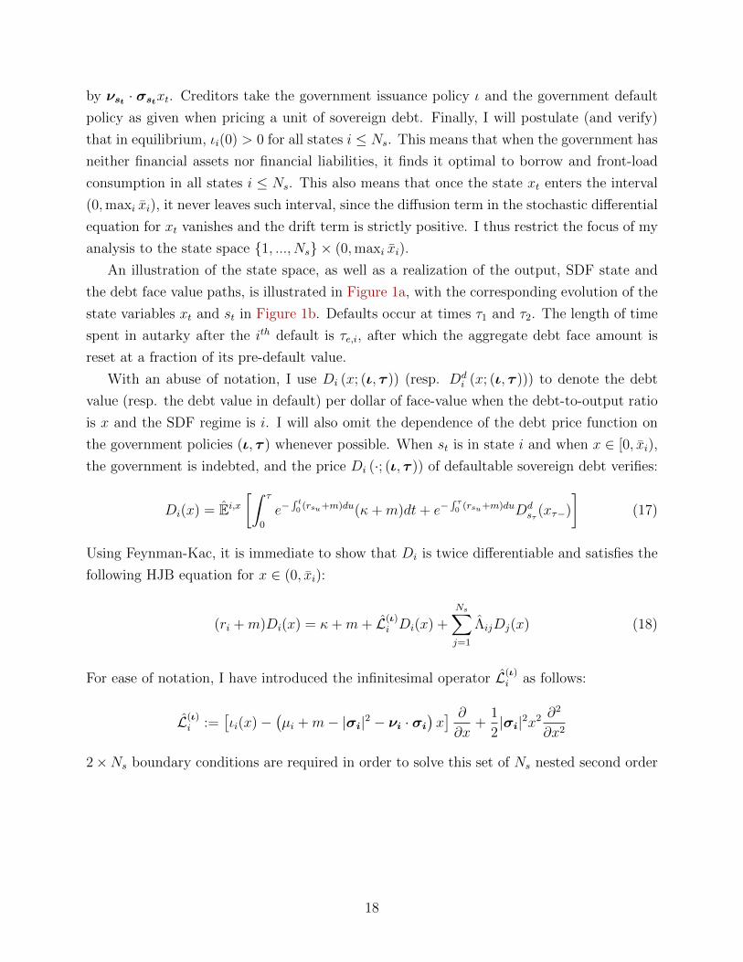
An illustration of the state space, as well as a realization of the output, SDF state and

the debt face value paths, is illustrated in Figure 1a, with the corresponding evolution of the

state variables xt and st in Figure 1b. Defaults occur at times τ1 and τ2. The length of time

spent in autarky after the ith default is τe,i, after which the aggregate debt face amount is

reset at a fraction of its pre-default value.

With an abuse of notation, I use Di (x; (ι, τ )) (resp. Ddi (x; (ι, τ ))) to denote the debt

value (resp. the debt value in default) per dollar of face-value when the debt-to-output ratio

is x and the SDF regime is i. I will also omit the dependence of the debt price function on

the government policies (ι, τ ) whenever possible. When st is in state i and when x ∈ [0, xi),

the government is indebted, and the price Di (·; (ι, τ )) of defaultable sovereign debt verifies:

Di(x) = Ei,x[∫ τ

0

e−∫ t0 (rsu+m)du(κ+m)dt+ e−

∫ τ0 (rsu+m)duDd

sτ (xτ−)

](17)

Using Feynman-Kac, it is immediate to show that Di is twice differentiable and satisfies the

following HJB equation for x ∈ (0, xi):

(ri +m)Di(x) = κ+m+ L(ι)i Di(x) +

Ns∑j=1

ΛijDj(x) (18)

For ease of notation, I have introduced the infinitesimal operator L(ι)i as follows:

L(ι)i :=

[ιi(x)−

(µi +m− |σi|2 − νi · σi

)x] ∂∂x

+1

2|σi|2x2 ∂

2

∂x2

2×Ns boundary conditions are required in order to solve this set of Ns nested second order

18

t

outp

utY

and

deb

tF

τ1 τ2

SD

Fst

ates

output Ytdebt FtSDF state st

(a) Output Yt and Debt Ft

x1

x2

x3

τ1

τe,1

τ2

τe,2

t

x

debt/GDP xtdefault boundary xst

(b) Debt-to-GDP ratio xt

19

ordinary differential equations. They are as follows, for 1 ≤ i ≤ Ns:

Di(xi) = Ddi (xi) (19)

(ri +m)Di(0) = κ+m+ ιi(0)D′i(0) +Ns∑j=1

ΛijDj(0) (20)

For each state i, the first boundary condition is a value matching condition, which says that

the debt price at the default boundary x = xi is equal to the price of a claim on the defaulted

debt, Ddi (xi) (which will be calculated later on). The second boundary condition is a Robin

boundary condition; it relates the value of the function Di at the origin to its first derivative

at the origin. It can be obtained by simply taking a limit of the HJB equation satisfied by

Di at x = 0. I need to compute the debt price in default Ddi (x), for x ≥ xi and 1 ≤ i ≤ Ns.

Assume that at time of default τ , the state is sτ = i. When the country exits financial

autarky, its debt-to-GDP ratio is equal to Fτ+τe

Yτ+τe= θFτ−

Yτ−= θxτ−. Note that it is possible

that xτ− > xsτ when the sovereign defaults. This happens upon the occurrence of a “jump-

to-default”, in other words a situation where the discrete SDF state jumps from sτ− = j to

sτ = i and when xi < xτ− < xj. Thus, I have the following for x ≥ xi:

Ddi (x) = Ei

[exp

(−∫ τe

0

rst+udu

)Ft+τeFt−

Dst+τe (θx)

]Section A.1.9 establishes the following formula for the defaulted debt price:

Dd(x) = λθαΞ−1D(θx) (21)

In equation (21), Dd(x) is the Ns× 1 vector with ith element Ddi (x), and the Ns×Ns matrix

Ξ := diagi (ri + νi · σi + λ− µi) − Λ is well defined thanks to Assumption 2. Finally, note

that this equation is valid for each coordinate i for x ≥ xi.

I end this section by discussing two different aspects of the model. First, the existence of a

discrete number of SDF regimes leads to two types of defaults: defaults following a sequence

of bad GDP shocks, as well as defaults induced by jumps in the SDF state, from a state of

low risk prices to a state of higher risk prices. Both types are illustrated in Figure 1a and

Figure 1b. In this example, a default occurs at τ1, after a sequence of bad GDP shocks that

cause the debt-to-GDP ratio to breach the optimal default boundary that the government

has set in such SDF regime. In the same figure, a default occurs at τ2, triggered by a jump

in the SDF state. At such time, an SDF regime shift occurs, from sτ2− = 3 to sτ2 = 2,

and the debt-to-GDP ratio satisfies x3 > xτ2− > x2. In other words, before the SDF jump,

the debt-to-GDP ratio of the sovereign is below the optimal default boundary, but as the

20

SDF regime shifts, the debt-to-GDP ratio is suddenly greater than the new optimal default

boundary, causing the sovereign to immediately default. Since the SDF I use will price the

sovereign debt of multiple countries, SDF regime shifts induce correlated defaults amongst

sovereign governments. Note that jump-to-default risk exists even if the GDP growth rate

and GDP growth volatility are not regime-dependent – so long as the SDF exhibits different

risk prices in different regimes.

Second, note that when x 0, the government debt balance is negligible compared to

output. However, the price of any infinitesimally small unit of debt is actually not equal to the

risk-free debt price, since the debt price needs to factor in the dilution risk of the government,

whose optimal issuance policy will dictate to issue debt to front-load consumption. This

observation is in stark contrast with what happens in structural corporate credit risk models

(see for example Leland (1994) or Leland (1998)) – in those models, the firm can commit to

a financing policy (typically, maintaining the debt face value constant), but cannot commit

to a default policy, leading to a debt price that is equal to the risk-free debt price when the

level of fundamentals becomes arbitrarily large compared to the debt face value.

3.5 Equilibrium Debt Issuance and Default Policies

Now consider the government’s problem, as described in Section 3.3. As a reminder, the gov-

ernment takes the debt price schedule D(·) as given when solving its optimization problem.

Thanks to Lemma 1, the government value function in state i can be written as follows:

Vi(Y, F ) := vi(x)Y 1−γ (22)

In the above, the function vi will be positive when γ ∈ (0, 1), and negative when γ > 1.

Since Vi is decreasing in F , I also have the sign restriction v′i(x) < 0. An appropriate change-

in-measure described in Section A.1.10 shows that the HJB equation associated with the

government problem, in the continuation region [0, xi), is the following:

1− γ1− ρ

Aivi(x)−Ns∑j=1

Λijvj(x) =

supιi

[δ

(1 + ιiDi(x)− (κ+m)x)1−ρ [(1− γ)vi(x)]ρ−γ1−γ

1− ρ+ L(ι)

i vi(x)

](23)

In the above, I have used the differential operator L(ι)i defined as follows:

L(ι)i :=

[ιi −

(µi +m− γ|σi|2

)x] ∂∂x

+1

2|σi|2x2 ∂

2

∂x2

21

The optimal state-contingent issuance policy ιi is then given by:

maxιi

[δ

1− ρ(1 + ιiDi(x)− (κ+m)x)1−ρ [(1− γ)vi(x)]

ρ−γ1−γ + ιiv

′i(x)

]This yields the (necessary and sufficient, given the strict concavity of the expression in

brackets w.r.t. ιi) first order condition:

Di(x)δci(x)−ρ [(1− γ)vi(x)]ρ−γ1−γ = −v′i(x) (24)

In the above, I have introduced the consumption-to-GDP ratio ci := C/Y when the discrete

Markov state is i. Focusing on equation (24), I notice that the left-hand side is the product

of (a) the marginal utility of consumption δci(x)−ρ [(1− γ)vi(x)]ρ−γ1−γ and (b) the debt price,

while the right-hand side is the marginal cost of taking on one extra unit of debt. The optimal

Markov issuance policy function ιi(x) is given by:

ιi(x) =1

Di(x)

(δDi(x) [(1− γ)vi(x)]ρ−γ1−γ

−v′i(x)

)1/ρ

+ (κ+m)x− 1

(25)

The expression is well defined since I showed previously that v′i(x) < 0. The dependence

of the issuance policy on the model parameters or on the debt price schedule (which the

government takes as given) are ambiguous, since those issuance parameters will also have a

feedback effect on the felicity function and its derivative. I can however perform a “partial

equilibrium” analysis of the debt price schedule in the unit elasticity of substitution case, i.e.

when ρ = 1. In such case, ιi(x) is an increasing function of Di(x) whenever the sovereign

output Yt is greater than the total debt service owed (κ + m)Ft, which will always be the

case in equilibrium (in other words in equilibrium, the sovereign will have defaulted before

the sovereign output falls low enough that new debt issuances are required to service the

existing debt). For the case where the elasticity of substitution is different from 1, I verify

numerically that this comparative static result still holds: when the debt price schedule is

more beneficial to the sovereign, the latter takes advantage of it through additional issuances.

For a given set of default thresholds xii≤Ns , 2×Ns additional boundary conditions are

needed do solve the system of Ns equations (23). The first set of conditions relates to value

matching at the default boundary xi. Let V di (Y, F ) be the government value function in

default, if the pre-default output level is Y and the pre-default debt face value if F . I show in

Section A.1.11 that V di (Y, F ) = vdi (xi) (αY )1−γ, which leads to the following value-matching

condition:

vi (xi) = α1−γvdi (xi) (26)

22

vdi (x) solves a system of non-linear equations discussed in Section A.1.11. I also have a set of

Ns Robin boundary conditions, linking the value function at the origin to its derivative, via:

1− γ1− ρ

Aivi(0)−Ns∑j=1

Λijvj(0) = δ(1 + ιi(0)Di(0))1−ρ [(1− γ)vi(0)]

ρ−γ1−γ

1− ρ+ ιi(0)v′i(0) (27)

I finally focus on the optimal default policy. Since it is always an option for the government

to default, I must have Vi(Y, F ) − V di (Y, F ) ≥ 0 for all states (Y, F ). This leads to a set of

Ns smooth-pasting conditions:

v′i (xi) = α1−γ(vdi )′(xi) (28)

Section A.1.11 establishes more formally this optimality condition and shows how (vdi )′(xi)

can be expressed as a function of vdi (xi) and vi(θxi). I conclude this section by two propo-

sitions. First, I establish a standard verification theorem for the government value function.

I then discuss the existence of a Markov perfect equilibrium, subject to the existence of a

solution to a set of ordinary differential equations.

Proposition 1. For any family of decreasing functions Di : R+ →[0, Drf

i

], assume that

there exists a family of functions vi (·;D) ∈ C1 (R+) ∩ C2 (R+ \ xi), which satisfies for

1 ≤ i ≤ Ns:

0 = max

[supι

[−1− γ

1− ρAivi (x;D) +

Ns∑j=1

Λijvj(x;D)

+δ(1 + ιiDi(x)− (κ+m)x)1−ρ [(1− γ)vi (x;D)]

ρ−γ1−γ

1− ρ+ L(ι)vi (x;D)

];α1−γvdi (x;D)− vi (x;D)

],

where vd (x;D) satisfies (using the Ns ×Ns matrix Υ := 1−γ1−ρdiagi (Ai) + λI − Λ):

Υvd(x;D)− λv(θx;D) =δ

1− ρ[(1− γ)vd(x;D)

] ρ−γ1−γ ,

Then for any state i ≤ Ns and any x ∈ R+, vi(x;D) ≥ Ji(1, x; (ι, τ );D) for any (ι, τ ) ∈I × T that satisfy limt→+∞ inf e−

∫ t0

1−γ1−ρAsuduvst

(x

(ι,τ )t ;D

)≤ 0. Let the family of thresholds

xi1≤i≤Ns ∈ (R+)Ns satisfy:

(vd)′

(xi) = λθ

(Υ + δ

γ − ρ1− ρ

diagj

([(1− γ)vdj (xi)

]− 1−ρ1−γ))−1

v′(θxi)

23

Let (ι∗, τ ∗) be defined as follows:

ι∗i (x;D) :=1

Di(x)

(δDi(x) [(1− γ)vi (x;D)]ρ−γ1−γ

−v′i (x;D)

)1/ρ

+ (κ+m)x− 1

τ ∗(D) := inft ≥ 0 : xt ≥ xst

Then vi(x;D) = Ji(1, x; (ι∗, τ ∗);D) is the value function.

This proposition, proven in Section A.1.12, provides for a characterization of the optimal

issuance and default policies given a decreasing debt price schedule D. It does not establish

the existence of an equilibrium, which is achieved in the next proposition.

Proposition 2. Assume that there exists a set of functions vi(·)i≤Ns , Di(·)i≤Ns , and

a set of positive thresholds xii≤Ns such that the system of nested ordinary differential

equations (18), (23) subject to value-matching boundary conditions (19), (20), (26) and (27)

are satisfied, where ιi(·) satisfies equation (25) and each threshold xi satisfies the smooth

pasting condition (28). Then a Markov perfect equilibrium exists.

Proving the existence of a Markov perfect equilibrium without relying on the (strong)

assumptions of proposition 2 is beyond the scope of this paper, and I leave this proof for

future research. I provide in Section A.1.13 a discussion of the potential route to pursue to

establish such result. I also show in Section 4, for the particular case where ρ = γ = 0, that

a Markov perfect equilibrium exists, and it is unique in the class of “smooth” equilibria (i.e.

equilibria in which the debt face value process is restricted to being absolutely continuous).

3.6 Asset Pricing Moments

In this section, I discuss the implications of my model for the long term sovereign bond

spread, as well as excess returns earned by international investors on such bond. I also show

how to compute CDS premia and the excess return on these contracts.

3.6.1 Long Term Sovereign Debt Spreads

The sovereign bond spread ςi(x) is the constant margin over the risk-free benchmark that

is needed to discount the long-term sovereign bond’s cash flow stream assuming away any

default risk. In other words, the credit spread must verify:

Di(x) := Ei,x[∫ ∞

0

e−∫ t0 (rsu+ςi(x)+m)du(κ+m)dt

](29)

24

The credit spread ςi(x) is the unique positive solution to the following equation:

Di(x) = (m+ κ)

[(diagj (rj + ςi(x) +m)− Λ

)−1

1

]i

Using Ito’s lemma, credit spread innovations under P take the following form:

dςt − E [dςt|Ft] = −ς ′st−(xt)xtσst− · dBt +∑s′

(ςs′(xt)− ςst−(xt)

) (dN (st−s′) − Λst−s′dt

)(30)

What happens upon the occurrence of a GDP shock? Section A.1.15 establishes that ς ′i < 0

in any state i. Thus, good GDP shocks translate into decreases in sovereign bond spreads.

In other words, credit spreads are counter-cyclical in this model – a sequence of good GDP

shocks will on average lead to lower spreads, consistent with empirical fact (4).

I can then leverage equation (30) to compute the instantaneous sovereign bond spread

volatility:

σςt =

√x2t |σst−|2ς ′st−(xt)2 +

∑s′

Λst−s′(ςs′(xt)− ςst−(xt)

)2(31)

In a model without SDF regime shifts, sovereign spread volatilities are purely driven by

the macroeconomic fundamentals of a country (in the context of this model, the debt-to-

GDP ratio x). Instead, SDF regime shifts in my model induce an additional component to

sovereign spread volatilities. A separate testable implication emerges from equation (31):

spread volatilies tend to be higher when the sovereign government is close to its endogenous

default boundary. Indeed, I show in the appendix that under mild conditions, the function

xς ′i(x) is increasing, meaning that the component of sovereign spread volatility stemming

from Brownian shocks increases as the sovereign government approaches its default cutoff.

Both predictions will be tested as part of my model validation.

Equation (30) also illustrates the crucial importance of the different SDF regimes for cross-

sectional spread correlations: absent those regime shifts, pairwise local spread correlation

between two different sovereign governments would only stem from output correlation, which

is at odds with fact (2). If I index by “a” and “b” two countries, the instantaneous spread

correlation between those countries takes the following form:

corrt (ςa,t, ςb,t) =ς ′a,st−ς

′b,st−

xa,txb,tσa,st− · σb,st− +∑

s′ Λst−s′(ςa,s′ − ςa,st−

) (ςb,s′ − ςb,st−

)σςa,tσ

ςb,t

In the formula above, for all states i ≤ Ns, the function ς ′a,i is evaluated at xa,t and the

function ς ′b,i is evaluated at xb,t. When the SDF state jumps from a low risk price level s to

a high risk price level s′, if both countries’ output processes are positively correlated with

25

the risk price vector in all discrete Markov states, spreads for both country “a” and country

“b” jump up, meaning that(ςa,s′ − ςa,st−

) (ςb,s′ − ςb,st−

)> 0. The same reasoning holds upon

a jump from a high risk price state to a low risk price state. Thus, the second term in my

formula for spread correlations above is positive: spread correlations are induced by SDF

regime shifts. This gives my model the potential for being consistent with fact (2) – but

only to the extend my countries of interest have output processes whose correlation with the

vector of risk prices have the same sign.

3.6.2 Long Term Sovereign Debt Returns

I then compute sovereign debt excess returns. Debt excess returns over the time period

(t, t + dt] include capital gains dDt, coupon payments κdt and principal repayments mdt,

while the opportunity cost is rstdt and reinvestment costs are equal mdt. Thus, excess

returns (under the physical measure P) are equal to:

dRet : =

dDt + (κ+m)dt

Dt

− (rst +m)dt

Using Ito’s lemma and the HJB equation satisfied by the family of debt values Di(·)i≤Ns ,I obtain expected excess returns (per unit of time) and return volatilities that are equal to:

E [dRet |Ft] = −

[xtD

′st(xt)

Dst(xt)νst · σst +

∑s′

Λsts′

(Ds′(xt)

Dst(xt)− 1

)(eυ(st,s′) − 1

)]dt (32)

var [dRet |Ft] =

x2tD′st(xt)

2

Dst(xt)2|σst|2dt+

∑s′

Λsts′

(Ds′(xt)

Dst(xt)− 1

)2

dt (33)

Thus, sovereign bond investors are compensated for taking Brownian risk (the first term on

the right hand-side of equation (32)), as well as for taking regime jump risk (the second

term on the right hand-side of equation (32)). The expected excess return can be read as

(minus) the local covariance between (a) sovereign debt returns and (b) the creditors’ pricing

kernel. This risk compensation is similar to a standard two-factor asset pricing compensation.

Indeed, I can interpret−xtD′st (xt)Dst (xt)

as the market beta of sovereign debt w.r.t. the shock Bt,

while νst · σst is the sovereign output claim’s risk premium earned in connection with such

shock. Similarly, the jump compensation (the second term in equation (32)) can be re-written:

∑s′

Λsts′

(eυ(st,s′) − 1

)(Ps′Pst− 1

)︸ ︷︷ ︸

output claim’s premium for jump risk

Ds′ (xt)Dst (xt)

− 1

Ps′Pst− 1

︸ ︷︷ ︸

market beta of sovereign debt w.r.t. jump risk

26

In the above, Pi is the price of a claim to the output of country i. Using the vector notation,

P =[diagi (ri + νi · σi − µi)− Λ

]−1

1. Alternatively, one can interpret those formulas using

the terminology of Hansen (2012a) or Hansen (2012b): in such case, the expected excess

return in equation (32) is the sum-product of (time-varying) risk prices (νst for the Brownian

shocks and(eυ(s,s′) − 1

)for jump risks) and (time-varying) risk exposures (

−xtD′st (xt)Dst (xt)

σst for

Brownian shocks and(Ds′Dst− 1)

for jumps).

Equation (32) highlights the crucial role of the local covariance between risk prices and the

GDP process for the determination of expected excess returns. When I tie the investor’s SDF

to US consumption growth and US consumption volatility (as in Section A.1.4), risk prices

are equal to the product of (i) US investors’ risk-aversion times (ii) US consumption growth

volatility. But US output and consumption growth exhibit only mild levels of correlation

with emerging market economies’ output growth, as documented in table “Country-Specific

Macro Moments” in the online appendix. One might then ask how this model might explain

the high level of expected excess returns earned on emerging market sovereign risks. Even if

the risk price vector νst is not (locally) correlated with the country’s output process, expected

excess returns can be positive when risk prices are time-varying and co-move with sovereign

debt prices. For this latter effect to “bite”, the pricing kernel must feature jumps (i.e. some

of the υ(i, j)1≤i,j≤Ns must be non-zero); the introduction of different SDF regimes only does

not suffice in order to produce large model-implied expected excess returns when νst ·σst ≤ 0

in all states.

Note also that the risk exposure to Brownian shocks (and the corresponding sovereign

debt market beta) depends on the elasticity−xD′i(x)

Di(x)of the bond price function. It turns out

that in all my numerical computations, the debt price function Di(·) is a concave function,

which means that the sovereign debt’s risk exposure to Brownian shocks is increasing in

x. This leads to another implication of the model: sovereign expected excess returns are

increasing in the debt-to-GDP ratio, consistent with fact (8). This implication was also

indirectly tested by Borri and Verdelhan (2011) when sorting sovereign debt portfolios by (a)

rating and (b) “market betas”, if one interprets the rating as a noisy measure of the debt-to-

GDP ratio. But while Borri and Verdelhan (2011) argue in the model section of their paper

that they would need to introduce two sources of heterogeneity in order to recreate their

empirical observation, I argue that this is not necessary: not only different countries may

have different business cycle correlations with foreign investors’ risk prices, but also countries

may have different risk exposures.

To conclude this section on long term debt returns, the properties of sovereign bond

return volatilities and cross-country correlations should be identical to those of sovereign

spread volatilies and cross-country sovereign spread correlations since realized bond returns

27

between t and t + dt are (approximately) proportional to spread changes during that time

period.

3.6.3 Credit Default Swap Premia and Returns

To conclude this section, I define ςi(x, T ), the credit default swap premium for a T maturity

contract. Conceptually, such premium should, at the time the trade is executed, compensate

the writer of protection for expected losses to be suffered on the contract. Mathematically,

ςi(x, T ) is defined as follows:

ςi(x, T ) :=Ex,i

[1τ<Te

−∫ τ0 rsudu max

(0, 1−Dd

sτ (xτ−))]

Ex,i[∫ T∧τ

0e−

∫ t0 rsududt

] =Li(x, T )

Pi(x, T )

Li(x, T ) is the risk-neutral expected credit loss, while Pi(x, T ) is the risk-neutral present-value

of CDS premia. Both expected losses and expected CDS premia can be calculated using the

Feynman-Kac formula, by solving a set of partial differential equations with boundary con-

ditions discussed in Section A.1.16. Section A.1.16 also provides formula for computing

expected excess returns and conditional return volatilities of CDS contracts of different ma-

turities. I can then test whether the model-implied term structure of spreads is consistent

with facts (5) and (6), and whether the term structure of expected excess returns is consistent

with fact (8).

My model with multiple SDF regimes (inducing multiple default boundaries, one per

regime) is particularly convenient in analyzing short term CDS premia, and confronting

them with the data. Indeed, when the CDS contract maturity is arbitrarily small (i.e. when

T → 0), default risk only stems from the risk of regime shifts. Under the assumption that

the discrete SDF states are ordered (i.e. under the assumption that x1 ≤ ... ≤ xNs), I then

have the following lemma, characterizing short term CDS premia.

Lemma 3. When the contract maturity T becomes arbitrarily small, the sovereign CDS

premium converges to the following limit:

limT→0

ςi(x, T ) =

0 if x ≤ minj xj or i = 1∑i−1j=1 Λij

(1−Dd

j (x))

otherwise

Lemma 3 shows that premium compensation for writers of short term sovereign CDS only

comes from SDF jump risk, as opposed to output volatility risk. In other words, a model that

28

does not feature multiple discrete SDF regimes would not feature high short-term market-

implied hazard rates, and would thus be inconsistent with stylized fact (3).

3.7 Macro Moments

One distinguishing feature of emerging market economies is the fact that the ratio of (a)

consumption growth volatility over (b) output growth volatility is substantially greater than

one (see for example Neumeyer and Perri (2005) or Aguiar and Gopinath (2004)). In my

model, as established in Section A.1.17, this ratio takes the following expression:

stdev[dCtCt

∣∣Ft]stdev

[dYtYt

∣∣Ft] =

√√√√(1−xtc′st(xt)

cst(xt)

)2

+1

|σst|2∑s′

Λst,s′

(cs′(xt)

cst(xt)− 1

)2

(34)

This ratio will thus crucially depend on how the consumption-to-output ratio ci(·) varies with

the debt-to-GDP ratio. As will be seen, as the debt-to-GDP ratio nears the default boundary,

the government will adjust its issuance policy downwards, meaning that the consumption-

to-output ratio ci(·) will be a decreasing function of x. This leads to a consumption growth

volatility that will be greater than output growth volatility. Note also that such volatility is

exacerbated by SDF regime shifts.

4 A Useful Benchmark: Risk-Neutral Goverment

The model presented above will need to be solved numerically, but there is one particular

parameter configuration where closed-form solutions are available: the case where the gov-

ernment is risk-neutral. Leveraging an insight from DeMarzo and He (2014), I develop in

Section A.1.18 the solution for this problem in the case where ρ = γ = 0. This benchmark is

useful to provide some intuition on the mechanics of the model.

Proposition 3. Assume that the government is risk-neutral, i.e. that γ = ρ = 0. Assume

that the risk-free rate in all SDF states is strictly less than the government’s rate of time

preference, i.e. ri < δ for all i ≤ Ns. Assume also that the GDP process is not regime-

specific, in other words assume that for all state i ≤ Ns, µi = µ and σi = σ. In such case,

there exists an equilibrium where the life-time government value function Vi(Y, F ), the debt

price schedule Di(Y, F ) and the optimal default cutoff xi are independent of the SDF state,

29

and have the following expressions:

D(x) =

(κ+m

δ +m

)[1−

(1− αθλ

δ+λ−µ

1− αθξλδ+λ−µ

)(xx

)ξ−1]

(35)

v(x) = δ

[1

δ − µ

(1−

(1− α

1− αθξλδ+λ−µ

)(xx

)ξ)− xD(x)

](36)

x =ξ

ξ − 1

(δ +m

κ+m

)( 1−αδ−µ

1− αθλδ+λ−µ

)(37)

In the above, ξ > 1 is a constant that only depends on the model parameters δ, µ,σ,m, and

not on the level of interest rates or the prices of risk. The scaled optimal financing policy

ιi(x) is SDF state-dependent and has the following expression:

ιi(x) =δ − riξ − 1

[(1− αθξλ

δ+λ−µ

1− αθλδ+λ−µ

)( xx

)ξ−1

− 1

]x− νi · σx (38)

The financing policy ιi(·) is a strictly decreasing function of x if δ+m > |σ|2− (m+µ), and

is otherwise hump-shaped. Conditional expected excess returns on the long-term bond have

the following expression:

E [dRet |Ft] =

ξ − 1(1− αθξλ

δ+λ−µ1− αθλ

δ+λ−µ

)(xx

)ξ−1 − 1

νi · σ (39)

The equilibrium above is the unique Markov perfect equilibrium featuring an absolutely

continuous debt face value process.

The first – and seemingly surprising – result of Proposition 3 is that the (output-normalized)

welfare value of a government without any debt outstanding (i.e. v(0)) is exactly equal to

the autarky welfare δ/(δ− µ). In other words, the fact that the risk-neutral government has

the option to take on debt financed by creditors with a discount rate that is strictly less than

the rate of time preference of the government is not welfare-improving for such government.

Similarly, when the government is indebted, the welfare of the government can be expressed

as the sum of (a) the welfare of a debt-free government that suffers a downward GDP drop

of (1 − α) % each time the state variable xt hits the boundary x, minus (b) the aggregate

value of sovereign debt, computed as if creditors were risk-neutral with a discount rate δ.

Importantly, neither the risk-free rates rii≤Ns , nor the price of risk νii≤Ns influence the

30

welfare value v(x):

V (Y, F ) = δ

Y

δ − µ

(1−

(1− α

1− αθξλδ+λ−µ

)(xx

)ξ)︸ ︷︷ ︸

value of “credit-risky” endowment

− FD(Y, F )︸ ︷︷ ︸aggregate debt value

This result is tightly related to the conjecture made in Coase (1972), and formally proven by

Stokey (1981) and Gul, Sonnenschein, and Wilson (1986), who show that a monopolist with

constant marginal costs selling a durable good to a continuum of consumers will actually

behave competitively, in the continuous-time limit, and not extract any monopoly rent. The

argument, in the context of the sovereign default model with a risk-neutral government,

works as follows: without commitment, no matter how many bonds the government sold in

the past, the government will sell more bonds if there are marginal gains from doing so (in

other words if those bonds can be sold at an implied interest rate strictly less than δ, i.e.

if δD(Y, F ) > −∂FV (Y, F )). But investors perfectly anticipate this behavior and thus price

the bonds at an implied interest rate of δ, therefore stripping away any potential welfare gain

that the government may extract from facing financiers that discount cash flows at a rate

strictly less than δ.

Note that this result is purely due to the continuous-time nature of my model; as high-

lighted by Stokey (1981) and as (unreported) computations illustrate, the discrete time coun-

terpart to this model would yield strictly positive welfare gains for the risk-neutral govern-

ment. Having a non-zero time period during which the government can commit not to issue

bonds is crucial in obtaining such result. Similarly, in the case of a risk-averse government,

the result above will no longer hold: the concavity in the flow payoff function will be such

that the government will extract welfare gains from issuing bonds to investors whose implied

interest rate is lower than the government’s rate of time preference. The country’s welfare,

sovereign bond prices and default boundaries will again depend on the level of risk-free rates

and prices of risk: since the government dislikes high levels of consumption volatility, its

financing policy will not fully adjust to keep sovereign bond prices unchanged; instead, the

adjustment will be partial. This result is analogous to what is showed theoretically in Kahn

(1986) in the context of the durable goods monopoly problem: rents can be extracted by the

monopolist if its marginal production costs are increasing.

As a consequence of Proposition 3, changes in the supply-side of capital lead the gov-

ernment to adjust its financing policy in such a way that sovereign bond prices and welfare

remain unchanged: with higher risk-free rates or higher prices of risk12, the higher financing

12This discussion assumes that the price of risk is positively correlated with the GDP process in all SDF

31

costs borne by the government are exactly compensated by a lower pace of debt issuances.

This translates into an upward adjustment of the country’s current account and trade bal-

ances, causing an endogenous sudden stop. In the context of an increase in the price of risk,

the magnitude of the current account reversal is high when the debt-to-GDP ratio of the

country is high. The financing policy of the government is also interesting to study since it

highlights the fact that when bond investors are risk-neutral (i.e. when the price of risk is

identically zero), the issuance policy of the government is always positive: it is never efficient

for the government to buy back debt. This result echos an insight from Bulow, Rogoff, and

Dornbusch (1988) who show, in the context of a one-period model of sovereign default with

a risk-neutral government and risk-neutral lenders, that it is never welfare-improving for a

country to buy back its own debt. This result breaks down in the presence of risk-averse

lenders, whose price of risk has a positive correlation with the country’s endowment process:

in such case, Equation (38) shows that there are parameter configurations where, for high

debt-to-GDP ratios, the country does find it optimal to buy back its own debt. For this to

be the case, the parameters of the model need to satisfy the following condition:

αλθ(1− θξ−1

)δ + λ− µ− αθλ

<ξ − 1

δ − riσ · νi

In other words, if either the price of risk |νi| is sufficiently high, or the GDP drop upon

default 1−α is sufficiently severe, or the risk-free rate ri is sufficiently close to the government

discount rate δ, it is sometimes optimal for the government to buy back debt. The key to this

result is the fact that the probability measure under which investors discount cash-flows (the

“risk-neutral” measure) is different from the probability measure (the “physical” measure)

under which the government optimizes. A different interpretation of this result can be put

as follows: persistent differences in beliefs about the growth rate of the country’s endowment

(where investors would be more “pessimistic” than the government) would also lead the

government to buy back debt when the debt-to-GDP ratio of the country is high.

Finally, the expected excess return earned on sovereign bonds is increasing in the debt-to-

GDP ratio, confirming the ability of the model to replicate – at least qualitatively – empirical

fact (8). In environments with constant risk-free rates, while an increase in the price of risk

induces a sudden stop, sovereign bond prices remain unchanged, leading to sovereign credit

spreads that are not reacting to these worse capital market conditions. Finally, the closed-

form expressions of Proposition 3 allow me to derive the following comparative static results.

Corollary 1. The default boundary x is decreasing in the impatience parameter δ, de-

states (i.e. νi · σ > 0).

32

creasing in the coupon rate κ, increasing in the GDP haircut post default 1− α, increasing

in the haircut parameter θ, decreasing in the expected autarky time 1/λ.

One particular comparative static result worth highlighting is the fact that the default

boundary (as well as the country’s welfare) is decreasing in the coupon rate κ. This will have

its importance when I analyze the Latin American debt crisis of the early 1980s – at that time,

most of the sovereign debt contracted by these small open economies was structured with

variable coupons indexed to US short term rates. As will be seen in Section 7, the increase

in short term rates creates a current account reversal that is magnified by the contractual

structure of sovereign debt at the time.

5 Applications

5.1 Numerical Illustration and Comparative Static Results

Before estimating my model for a set of countries of interest, I first provide some comparative

static analysis, in order to gain some intuition about the role of certain model parameters.

To facilitate this investigation, I shut down for now the multiple SDF regimes, and analyze

the effect of certain model parameters in an environment where there is only one SDF regime.

I solve the model numerically using a Markov chain approximation method, as described in

details in Section A.3.

5.1.1 Calibration

Table 1 highlights the base case parameters I use for this comparative static analysis. I select

model parameters that are meant to represent the “average” emerging market economy of

the dataset studied in the online appendix. More specifically, the table “Country-Specific

Macro Moments” in the online appendix, constructed using data from the World Bank, shows

that the average real GDP growth rate for the countries in my dataset is 3.5% p.a., and the

average real GDP growth volatility is 4.1% p.a., leading to the parameters µ and σ in Table 1.

In the same online appendix, the table “Bond Issuance Average Maturities” shows summary

statistics for a dataset of foreign currency sovereign bonds I collected from Bloomberg13;

according to such table, the average original maturity date of sovereign bonds issued by my

13For all countries in the data-base I construct, I download all bonds listed on Bloomberg and issued bysuch country. I only keep in my data-base foreign currency bonds denominated in either EUR, GBP, USD,JPY or DEM. I also exclude bonds whose original notional amount is less than USD 100mm, whose originalterm is less than 1 year or greater than 50 years, or bonds with non-fixed coupon rates. The list of remainingbonds is available upon request.

33

Parameter Value Description1/ρ 0.5 IESγ 5 Risk aversionδ 0.2 Rate of time preferenceµ 0.035 GDP growth rate|σ| 0.04 GDP growth volatility

1− α 0.04 GDP % fall at default1/λ 5 Capital markets’ exclusion (years)θ 0.50 Debt-to-GDP upon autarky exitr 0.05 Creditors’ risk free rate|ν| 0.625 Creditors’ market price of risk

corr(ν,σ) 0.50 Business cycle-risk price correlation1/m 7 Debt average life (years)κ 0.05 Debt coupon rate

Table 1: Calibration Parameters

sample of 27 emerging market countries is 13.8 years. Since a country consistently rolling over

13.8-year original maturity bonds has a debt average life of 6.9 years, I pick 1/m = 7 years.

I select jointly the default punishment parameter 1− α and the rate of time preference δ to

approximately match two moments of the data: the average debt-to-GDP ratio (equal to 50%

for the set of countries of focus, as indicated in the “Country-Specific Macro Moments” table

in the online appendix), and the average 5yr CDS premium (equal to 395bps for the set of

countries of focus, as indicated in “Country-Specific Debt Price Moments” table in the online

appendix). This procedure yields a permanent output drop upon default of 1 − α = 4%14,

and sovereign rate of time preference δ = 20%. According to Tomz and Wright (2013), it

takes 4.7 years post-default for a country to regain access to capital markets, leading me to

pick 1/λ = 5 years. Benjamin and Wright (2009) find a mean creditor haircut following a

sovereign default of approximately 40%. Since my model assumes that the face value of debt

at exit from financial autarky is equal to θYτ+τe/Yτ− times the face value of debt pre-default,

the model-implied face value haircut is equal to:

1− θαE[e(µ−

12σ2)τe

]= 1− αθλ

λ−(µ− σ2

2

)14Note that estimates of output drops following a sovereign default vary vastly across the empirical litera-

ture: Hebert and Schreger (2016) for example calculate the cost of Argentina’s sovereign default to correspondto 9.4% permanent reduction in output; Aguiar and Gopinath (2006) use a (transitory) cost of default of 2%of output in their model, citing evidence from Rose (2005), who calculates an 8% decline in internationaltrade following a sovereign default.

34

I thus pick θ = 0.50, leading to a model-implied average creditor haircut of 42%. I choose

an inter-temporal elasticity of substitution equal to 1/ρ = 0.5 that is consistent with the

international business cycle literature15, and a risk-aversion parameter γ = 5 that is consistent

with the asset pricing literature. Risk-free rates are set at 5% p.a., and I pick a sovereign debt

coupon rate of 5%, which means that (a) the risk-free value of government debt is 1, and (b)

the sovereign debt always trades at a discount to par. The magnitude of the risk price ν is

set at the ergodic mean risk price of Lettau and Wachter (2007) (the pricing kernel I will use

later on when incorporating multiple SDF states). In a model with one risk price state (and

therefore no SDF jumps), |ν| corresponds to the highest Sharpe ratio attainable by any asset

priced by international investors (see Hansen and Jagannathan (1990))16. To start with, I

assume a correlation between the creditors’ risk price and the government’s output process

of 50%, and will discuss how this correlation affects equilibrium outcomes in Section 5.1.3

(of course in this simple model, varying this correlation and keeping risk prices constant is

equivalent to keeping this correlation constant and varying risk prices). In all the figures I

will be discussing, I plot in dotted lines the ergodic distribution of the state variable xt in

order to focus my attention on the sub-interval of the state space where I expect to see most

of my model-implied observations. This ergodic distribution is obtained via integrating a set

of Kolmogorov forward equations, as Section A.1.14 reveals. In the case of a unique SDF

regime, the ergodic distribution admits the following semi-closed form expression:

Lemma 4. In the absence of multiple SDF states, the ergodic distibution f takes the following

form:

f(x) =

∫ xθx

exp[∫ t

x2

|σ|2s2 ((m+ µ)s− ι(s)) ds]

2G|σ|2t2dt if x ∈ [0, θx)∫ x

xexp

[∫ tx

2|σ|2s2 ((m+ µ)s− ι(s)) ds

]2G|σ|2t2dt if x ∈ (θx, x)

The constant G is pinned down by the condition∫ x

0f(x)dx = 1− 1

1+λT (θx), where T (x) is the

expected default time conditional on the initial debt-to-GDP ratio being equal to x.

5.1.2 Base Case Calibration Equilibrium

In Table 2, I display the key model-implied moments of interest, as well as the target and

historical values for the “average” of my 27 countries in the online appendix. The base case

15Aguiar et al. (2016b), Aguiar and Gopinath (2006), Arellano (2008) all use an IES of 0.5.16Note that this 62.5% maximal Sharpe ratio is slightly higher than the unconditional Sharpe ratio of 40%

obtained for US equities – computed using an historical average of US equity market excess returns of 6%,and a yearly volatility of 15%.

35

Target/Moment Notation Value Historial Valuedefault boundary x 56%mean debt-to-GDP E [xt] 52% 50%stdev debt-to-GDP stdev [xt] 3% 24%consumption-output vol ratio vol (Ct) /vol (Yt) 1.94

default rate (1/λ+ T (θx))−1 2.8% p.a.bond spread E [ς(xt)] 365 bps p.a.5y CDS spread E [ς(xt, 5)] 414 bps p.a. 407 bps p.a.5y-1y CDS slope E [ς(xt, 5)− ς(xt, 1)] 60 bps p.a. 72bps p.a.bond excess return E [dRe

t ] 164 bps p.a.bond return volatility stdev [dRe

t ] 525 bps p.a.5y CDS excess return E

[dRe

t,5

]230 bps p.a. 508 bps p.a.

5y CDS return volatility stdev[dRe

t,5

]732 bps p.a.

Table 2: Base Case Calibration Results

calibration results in an optimal debt-to-GDP default boundary x = 56%, an ergodic mean

debt-to-GDP ratio of 52% and an ergodic debt-to-GDP distribution standard deviation of

3.0%. In Figure 2, I plot the issuance policy ι and the resulting trade balance. The issuance

policy is a decreasing function of the debt-to-GDP ratio, positive but reaching levels close

to zero at the default boundary. It is important to keep in mind that these represent gross

issuances, before taking into account any debt amortization. In Figure 2a, the dotted blue line

represents the locus of points (µ+m− |σ|2)x, i.e. the required value of ι(x) such that the

drift rate of x is zero. It is immediate to notice that the debt-to-GDP ratio is a mean-reverting

variable – its drift rate is going to be positive for values of x on the left of the intersection

of the solid and dotted blue lines and negative on the right side of such intersection. The

resulting trade balance (as a fraction of GDP) is equal to 1 − c(x) = (κ + m)x − ι(x)D(x).

It is negative for low debt-to-GDP levels and positive otherwise. Thus, consistent with

the overwhelming data for emerging market economies, the trade balance in this model is

countercyclical.

Since the consumption-to-output ratio c(x) is a decreasing function of the debt-to-GDP

ratio, using equation (34) it is immediate to see that the model generates a consumption

growth volatility that is greater than output growth volatility, an empirical regularity of the

data. For the parameters selected, I obtain an ergodic consumption growth vol to output

growth vol ratio of 1.94, which is in line with several emerging market economies, as docu-

mented in Aguiar and Gopinath (2004)17. Note also that consumption growth and output

17They find a ratio of 1.38 for Argentina, 2.01 for Brazil, 2.39 for Ecuador, 1.70 for Malaysia, 1.24 forMexico, 0.92 for Peru, 0.62 for the Philippines, 1.61 for South Africa, 1.09 for Thailand and 1.09 for Turkey.

36

Figure 2: Government Financing Policy and the Trade Balance

(a) Gross Issuance Policy ι(x) (b) Trade Balance 1− c(x)

growth are perfectly correlated (at least locally) in a model with one SDF regime, which is

obviously counter-factual – the model featuring multiple SDF regimes breaks this result.

I plot the sovereign bond price and the sovereign spread in Figure 3. The ergodic mean

credit spread of the exponentially amortizing bond is equal to 365bps p.a., and the ergodic

credit spread volatility is equal to 132bps p.a. This ergodic mean credit spread volatility is

higher than what is obtained by Aguiar et al. (2016b) and the difference stems from the much

lower average maturity of sovereign debt (2 years) this latter article assumes, compared to

the 7-year average life debt in the data for my countries of interest.

Focusing on Figure 3, bond prices decrease with the debt-to-GDP ratio, while bond

spreads increase. Even at low debt-to-GDP ratios (i.e. lower than the ergodic debt-to-GDP

mean), sovereign spreads are far from negligible. When the sovereign has no debt outstanding,

sovereign spreads are strictly positive – a simple manipulation of equation (20) shows that

the sovereign spread at x = 0 verifies:

ς(0) = −ι(0)D′(0)

D(0)

This equation highlights the role of future debt issuances (and the implicit dilution risk

associated with those future debt issuances): at low debt-to-GDP ratios, creditors perfectly

anticipate that the government will be issuing large amounts of debt (since the government

37

Figure 3: Government Bond Prices and Spreads

(a) Bond Prices D(x) (b) Bond Spreads ς(x)

is impatient), leading them to price bonds at a discount that reflects such dilution risk.

I then focus on credit default swap premia ς(x, T ). While the government uses 7-year

bonds to smooth and front-load consumption, my model allows me to compute the premium

ς(x, T ) of CDS contracts at any time-horizon T , as discussed in Section 3.6. The numerical

procedure to solve the relevant PDEs is described in details at the end of Section A.3. I plot

CDS premia in Figure 4a for 1-year, 3-year and 5-year contracts, and I plot in Figure 4b the

5y-1y slope. CDS premia for short-dated contracts are close to zero when the debt-to-GDP

ratio is far away from the mean ergodic debt-to-GDP ratio, highlighting the fact that at such

low debt-to-GDP levels, the sovereign slowly increases its indebtedness, such that 1-yr credit

instruments are almost risk-free. The 5-year CDS premium ς(x, 5) resembles the credit spread

of the exponentially amortizing bond ς(x) used by the government to finance itself, since the

average life of this bond is 7 years. Lastly, the term structure of credit spreads becomes

inverted as the sovereign approaches its default boundary. This property of my model ends

up being a very general property of default models that are structured as “first-hitting-time”

models, where the state is mean-reverting and has continuous sample paths. This feature of

the model also fits with stylized fact (5).

I plot in Figure 5 the bond expected returns and the bond price elasticity. Expected excess

returns are non-zero, since I have used a pricing kernel that co-moves with the country’s

output process: the unconditional expected excess return is equal to 1.64% p.a., while the

38

Figure 4: Credit Default Swap Premia

(a) CDS ς(x, T ) (b) CDS Slope ς(x, 5)− ς(x, 1)

Figure 5: Expected Excess Returns and Bond Price Elasticity

(a) Expected Excess Returns (b) Bond Price Elasticity −xD′(x)

D(x)

39

unconditional return volatility is equal to 5.25% p.a. Expected excess returns increase with

the debt-to-GDP ratio, since the bond price function’s elasticity increases with the state

variable x – this is the model counterpart to fact (8) in the data. I plot the bond price

elasticity −xD′(x)D(x)

in order to get a better understanding of the magnitude of the sovereign

bond’s US equity market beta – this will help me understand whether my model stands a

chance at generating the magnitude of expected excess returns observed in the data. In the

one-state SDF model, conditional expected excess returns are equal to −xD′(x)

D(x)σ ·ν. The risk

prices will be time-varying in the full model, but will on average be equal to 62.5%. Most

of my countries of interest have GDP volatilities of the order of 4%, meaning that at best,

an emerging market output’s risk premium is equal to σ · ν ≈ 2.4%. In this one-state SDF

model, the bond price elasticity has an ergodic average equal to 1.33. Thus, at best (in other

words when corr (ν,σ) = 1), the ergodic mean excess return will be equal to 3.3% – high,

but not quite sufficient to reach the unconditional expected excess returns in the data for

certain countries such as Brazil or Hungary for example.

I end this section by focusing on the historical measure. When the country emerges

from financial autarky, it has a debt-to-GDP ratio θx = 28.5%, and it takes such country

on average 24 years to default on its debt, once it has exited from autarky. The sovereign

default frequency under the physical measure is thus equal to 2.8% p.a. – slightly higher

than the unconditional estimate of 2% cited in multiple studies, but this measure is of course

extremely difficult to estimate accurately in the data given the low frequency nature of

sovereign defaults18.

After having investigated some of the key outputs of the model in the base case parametriza-

tion, I now study the impact of the model parameters on various endogenous quantities of

interest. This comparative static analysis will be used in my estimation in order to provide

identification for a subset of parameters of my model.

5.1.3 Comparative Statics

Table 3 is a summary of the comparative statics with respect to several parameters of the

model. These comparative statics are performed starting from the base case parametriza-

tion of Table 1. In the table, I compute the elasticity of the moment of interest w.r.t. the

parameter of interest; blue numbers correspond to positive elasticities, red numbers corre-

18It is also worthwhile noting that this historical default frequency is high due to the assumption that theloss severity suffered by bond investors in connection with a sovereign default is not 100%. In the discrete timeliterature on sovereign defaults, barring a few exceptions, most papers assume that creditors’ loss severityupon a sovereign default is 100%. In the case of creditors’ risk-neutrality, this automatically causes the levelof credit spreads to be close to the level of historical default intensities; if instead a recovery R is realizedby creditors, the historical default intensity would be approximately 1/(1 − R) times the average sovereigncredit spread.

40

spond to negative elasticities. As an example, if one focus on the ergodic debt-to-GDP mean

and the variation of such mean w.r.t. the impatience parameter δ, the elasticity is equal

to ∂ lnE[xt]∂ ln δ

= −0.56, meaning that a 10% increase in the value of the parameter δ leads to

5.2% decrease in the ergodic mean debt-to-GDP ratio. These elasticities are closely related

to the covariance matrix of parameter estimates that will be calculated as part of my model

estimation.

The GDP drop upon default 1 − α has a significant impact on government behavior –

specifically on the debt-to-GDP ratio at default, its ergodic mean and standard deviation.

An increase in the default punishment incentivizes the government to support higher levels

of debt in equilibrium, a result already known in the literature using discrete time models.

The magnitude of the sensitivities are not surprising: my output process being a geometric

Brownian motion, any downward GDP drop is a permanent shock that is translated into

large welfare losses. Since the default boundary increases with the magnitude of the GDP

drop post-default, the government issuance policy adjusts upwards, via an almost-parallel

shift.

As the government becomes more impatient (i.e. as δ increases), it tends to front-load

consumption when it is not significantly indebted. The impatient government thus has a

debt issuance policy with a steeper slope than the patient government, and the optimal

default boundary is lower for the former than for the latter. With an impatient government,

creditors take into account the dilution risk and price the debt more punitively than in the

situation where the government is patient, which leads to higher credit spreads, and a much

steeper 5yr-1yr spread slope. The long-run mean spread volatility is higher, which leads to

significantly higher risk-premia.

My framework allows me to investigate the separate roles of risk-aversion and inter-

temporal elasticity of substitution in the government’s decision problem – an analysis that the

international macroeconomic literature has not focused on so far. An increase in risk-aversion

tends to decrease the debt issuance rate, due to a greater precautionary savings motive.

It also increases the incentive to default, since welfare costs of business cycle fluctuations

increase with the level of risk-aversion, and since consumption volatility is greater than

output volatility in this class of models. Thus, the equilibrium default boundary is lower

with a more risk-averse government.

Increases in GDP volatility decrease the equilibrium debt-to-GDP default boundary. Once

again, this is due to the increase in the incentive to default, since welfare costs of business

cycle fluctuations increase with the GDP volatility, and since consumption volatility is greater

than output volatility. The mean bond spread increases significantly, since if one keeps the

government financing policy unchanged, a greater GDP volatility increases the default barrier

41

hitting probabilities (of course there will be an equilibrium response by the government, which

will reduce its debt issuances). A greater GDP volatility increases bond spread volatilities,

and as expected the sovereign bond risk-premium is materially higher. More surprisingly, a

greater GDP volatility does not lead to a meaningfully wider debt-to-GDP distribution, as

illustrated by the low sensitivity of stdev [xt] to |σ|. This is disappointing since it suggests

that stochastic volatility will not rescue one fundamental weakness of this class of models: the

fact that the model-implied ergodic debt-to-GDP distribution is a lot thinner than the one

observed in the data – the latter being computed and displayed in table “Country-Specific

Macro Moments” in the online appendix.

5.1.4 Breaking Down Governments’ Cost of Financing

In order to better understand the impact that SDF regime shifts will have on equilibrium

outcomes, I look at the comparative static w.r.t. ν in more details. Higher risk prices in-

crease sovereign spreads, lower government bond prices, leading the government to adjust

its issuance policy downwards. Higher creditors’ risk prices also cause the sovereign govern-

ment to default at lower debt-to-GDP levels – although the adjustment is relatively small.

This mechanism leads, in a multi-SDF-regime version of my model, to jump-to-default risk,

induced by risk prices jumping from one level to another (higher) level. When comparing

credit spreads for ν = 0 to credit spreads with strictly positive risk prices, one might want to

interpret the spread differential between those two parameter configurations as the “spread

premium” that a sovereign government is paying to its creditors above and beyond what

would be actuarially fair. This is not exactly the case since the government endogenously

reacts to those higher risk prices by altering its issuance and default policies.

I thus look at the following credit spread decomposition: starting from the equilibrium

without risk-pricing, I first adjust risk prices to |ν| = 0.625 (and under the assumption thatν·σ|ν||σ| = 0.50) and re-compute sovereign debt prices and spreads, keeping the government’s

issuance policy constant. I then adjust the government’s issuance policy to reflect such

government’s “best response” to this new debt price schedule. I will use this decomposition

in Section 6 in order to compute the cost borne by governments when issuing bonds to risk-

averse (US-based) investors. As discussed, this cost cannot be computed by simply evaluating

the average excess return paid to creditors for taking on sovereign credit risk, given the fact

that sovereign issuance policies depend on investors’ risk attributes; a counterfactual analysis

is required to decompose this sovereign financing cost.

The result of such decomposition is illustrated in Figure 6: the credit spread function

plotted in red is the spread under the intermediate step where risk prices are set to 0.625

but where the government issuance policy has not reacted yet. Figure 6 shows that positive

42

Figure 6: Credit Spread Decomposition

risk prices alone act as a powerful force to push credit spreads wider. Indeed, when |ν| is

increased from zero to |ν| = 0.625 (and the issuance policy is not adjusted), the drift rate of

the state variable xt increases by xtσ ·ν ≈ 0.5×0.04×0.625×0.5 = 0.625% per annum (using

the ergodic debt-to-GDP ratio for xt and the assumed 50% correlation between risk prices

and GDP), and the credit spread is wider by 233bps p.a. on average (this can be seen in the

plot by the upward shift from the curve ν = 0 to the curve ν = 0.625∗). But the government

responds by adjusting its issuance policy downwards, defaulting at a lower debt-to-GDP

burden, and the resulting credit spreads ends up wider by “only” 101bps p.a. on average

(using the ergodic distribution with risk-pricing). In other words, in this simple calibration,

101/360 ≈ 28% of total financing cost of the government is attributable to investors’ risk

aversion. For my panel of countries of interest, as will be seen shortly, this cost will turn out

to be very close to 30%.

6 Structural Estimation

6.1 Procedure

I select a subset of N = 8 countries out of the set of 27 countries discussed in the online

appendix and for which I have the longest time-series data available. My subset consists

of Brazil, Bulgaria, Hungary, Indonesia, Mexico, Philippines, South Africa and Turkey. My

43

model with SDF regime shifts has a large number of parameters to determine. I am going

to impose restrictions on those parameters as follows. First, I will use a pricing kernel

specification widely used in the asset pricing literature to rationalize properties of US equity

market returns: the pricing kernel of Lettau and Wachter (2007), originally built to explain

(amongst other things) the value premium. This SDF features a constant risk-free rate (2%

per annum), and risk prices that follow an AR(1) process. Section A.4 provides a detailed

description of the properties of this SDF, as well as the method I use to transform the original

continuous-state specification of Lettau and Wachter (2007) into a discrete state continuous-

time Markov process νstt≥0, using a numerical procedure based on matching conditional

and unconditional moments of the original model and the approximating model. This gives

me the risk free rates rii≤Ns , risk prices νii≤Ns , the matrix of intensities Λ as well as the

SDF jumps υ(i, j)i,j≤Ns . I choose a number of states Ns = 5 in order to be able to solve

for a single equilibrium of my model in a few minutes of computing time. My risk prices

νii≤Ns are equally spaced between 0% and 150%, with an ergodic mean of 62.5%.

The remaining parameters to estimate are country-specific. For simplicity and due to the

small number of GDP data points available, I will assume that for each country of interest,

expected consumption growth, consumption growth volatility and the correlation between

the country’s output process and the SDF risk price do not change with SDF regime shifts,

in other words for each country n, µni = µnj , σni = σnj andσni ·νi

|σni ||νi|

=σnj ·νj

|σnj ||νj |

for any pair of SDF

states i, j. I will also assume that the sovereign government has time-separable preferences,

in other words I will assume that γn = ρn for each country n. A few other parameters are

calibrated using a-priori evidence. I will leverage the average original maturity of bonds

issued by each country (as documented in the “Bond Issuance Average Maturities” table

in the online appendix) in order to calibrate the debt parameter mn for country n19. The

expected time spent in financial autarky 1/λ and the parameter θ governing the debt-to-GDP

post-autarky are kept at their values in Table 1 and are thus not country-dependent. For each

country n, my estimation will then pin down the GDP growth µn, GDP volatility |σn|, the

preference parameter γn = ρn, the correlation between GDP and the risk price vector ν·σn

|ν||σn| ,

the GDP drop upon default 1− αn and the rate of impatience δn. The following 6 moments

will be used in my estimation. First, the first difference mean and standard deviation of log

output will provide information on µn and |σn|. Unconditional expected excess returns on 5y

CDS contracts will then provide information on the correlation between country n’s output

and risk prices. Finally, the level of 5y CDS premia, the mean debt-to-GDP ratio and the

term structure slope (i.e. the difference between 5y CDS and 1y CDS spreads) will jointly

19A country consistently rolling over T -year original maturity bonds has a debt average life of T/2 years;for such country I thus use λ = 2/T .

44

provide information on 1− αn, δn and γn.

My simulated method of moment estimation follows closely Lee and Ingram (1991).

I note H = 1T

∑Tt=1 ht the p × 1 vector of target moments in the data, and Hk(Θ) =

1T

∑Tt=1 h (xnt n≤N , st; Θ) the corresponding p × 1 vector of moments generated by the kth

simulation of my model. I use K = 1000 simulations, and note H(Θ) = 1K

∑Kk=1Hk(Θ)

the sample average of moments generated by my model across the K simulations. For each

simulation, I use an identical seed and generate 2T years of data, burn-in the first T years,

keeping only the simulated data for the last T years. I minimize the criterion function:

Θ = arg minΘ

(H −H(Θ))′W (H −H(Θ))

I use the diagonal matrix W = (diagi (H2i ))−1

as my weighting matrix, to penalize propor-

tional deviations of the model-implied moments from their data counterparts. I compute the

asymptotic covariance matrix of my estimator as follows:

covar(

Θ)

=1

T

(1 +

1

K

)(∂H∂Θ

′W∂H∂Θ

)−1∂H∂Θ

′W ′ΩW

∂H∂Θ

(∂H∂Θ

′W∂H∂Θ

)−1

In the above, Ω is a consistent estimator of the long run covariance matrix of the moment

conditions Ω =∑+∞

j=−∞ E[(ht − E [ht]) (ht−j − E [ht−j])

′]. Since my moments of focus are

computed using different data sets, over different time periods and with different frequencies

of data available, computing a consistent estimator of Ω (using Newey and West (1986) for

example) is difficult. Thus, instead, I compute an estimator of Ω using the null of my model:

Ω(Θ) :=1

K

K∑k=1

(Hk (Θ)−H (Θ)) (Hk (Θ)−H (Θ))′

Under the null hypothesis, Ω(Θ) is a consistent estimator of Ω.

6.2 Results – the Case of Brazil

In Table 4 and Table 5, I first display the parameter estimates, then the target and model-

implied moments, and finally additional moments that were not targeted in my estimation.

I display in figures 7, 8 and 9 the equilibrium outcome for Brazil. In the highest risk price

state, Brazil defaults at a debt-to-GDP ratio of 34.8%, whereas in the lowest risk price state,

it defaults at a debt-to-GDP ratio of 36.3%, illustrating the relatively small impact of risk

prices on optimal default boundaries.

Figure 7 highlights the endogenous response of Brazil’s financing policy, trade and current

45

account balance to changes in international financial market conditions. Upon an increase

in the price of risk, its bonds trade at steeper discounts, inducing Brazil to reduce its debt

issuances. Jumps from the lowest risk price state to the highest risk price state lead to a large

adjustment to the current account and trade balances of approximately 4% of GDP. Thus,

increases in international risk prices constitute an endogenous mechanism for generating

sudden stops. Across my model economies, the adjustment in the trade and current account

balances varies beween 3% and 5%. While this is not sufficient to explain the full adjustments

observed in South East Asia post 1997 in connection with the Asian Tiger crisis (as illustrated

in Figure 16), those adjustments are nonetheless material. The mechanism used to generate

endogenous sudden stops in this paper thus differs from the more standard channel that has

been investigated in the past by the international macroeconomics literature – occasionally-

binding borrowing constraints in RBC models, such as those featured in Mendoza (2002) or

Mendoza (2010), and which depress investment and output when the small open economy

suffers a sequence of bad fundamental shocks and bounces against such constraint.

Figure 8 then shows that 5yr CDS levels jump up with transitions from low risk price

states to high risk price states – at the mean of the debt-to-GDP ratio ergodic distribution

for example, 5yr CDS jumps by more than 300bps between the lowest and the highest risk

price states. The term structure of credit spreads may invert for two reasons according to

Figure 8b: either following a sequence of bad fundamental shocks that push Brazil’s debt-

to-GDP ratio closer to the relevant default boundary, or upon an upward shift in risk prices.

This feature of the model is thus consistent with the data, as suggested by facts (5) and (6).

Figure 9 illustrates aspects of my model that are consistent with facts (7) and (8). Indeed,

one can see that CDS expected excess returns increase with the debt-to-GDP ratio, which

was expected given that the elasticity of the bond price function is increasing in the debt-

to-GDP ratio (this is fact (7)). In addition, longer-term CDS contracts earn higher excess

returns than shorter-term CDS contracts, for a given debt-to-GDP level and a given risk

price level (this is fact (8)). This effect is due to the risk exposure of CDS contracts, which

is increasing in the tenor of such contract.

Table 4 and Table 5 also indicate the estimated average bond spread (for the exponentially

amortizing long term bond issued by each small open economy), as well as the average bond

spread that would prevail if investors were instead risk-neutral (in row titled “Bond spread

– RN model”). The difference between those two spreads can thus be viewed as the excess

compensation paid to sovereign debt investors for taking on risks that are correlated with

those investors’ marginal utility process. On average, approximately 30% of the credit spread

paid by sovereign governments above and beyond the risk free rate is attributable to investors’

risk aversion.

46

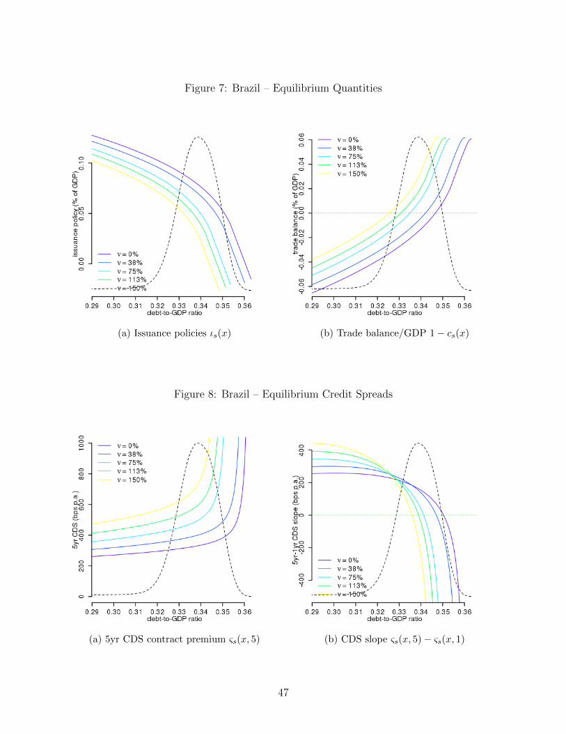
Figure 7: Brazil – Equilibrium Quantities

(a) Issuance policies ιs(x) (b) Trade balance/GDP 1− cs(x)

Figure 8: Brazil – Equilibrium Credit Spreads

(a) 5yr CDS contract premium ςs(x, 5) (b) CDS slope ςs(x, 5)− ςs(x, 1)

47

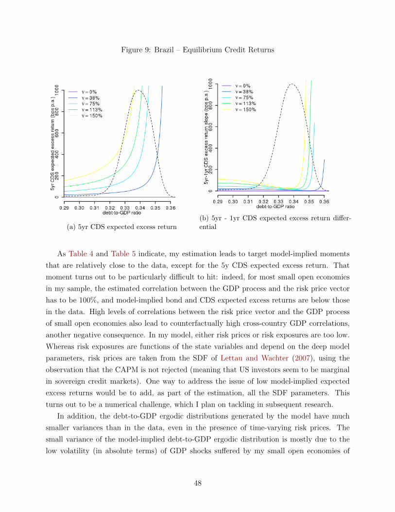
Figure 9: Brazil – Equilibrium Credit Returns

(a) 5yr CDS expected excess return(b) 5yr - 1yr CDS expected excess return differ-ential

As Table 4 and Table 5 indicate, my estimation leads to target model-implied moments

that are relatively close to the data, except for the 5y CDS expected excess return. That

moment turns out to be particularly difficult to hit: indeed, for most small open economies

in my sample, the estimated correlation between the GDP process and the risk price vector

has to be 100%, and model-implied bond and CDS expected excess returns are below those

in the data. High levels of correlations between the risk price vector and the GDP process

of small open economies also lead to counterfactually high cross-country GDP correlations,

another negative consequence. In my model, either risk prices or risk exposures are too low.

Whereas risk exposures are functions of the state variables and depend on the deep model

parameters, risk prices are taken from the SDF of Lettau and Wachter (2007), using the

observation that the CAPM is not rejected (meaning that US investors seem to be marginal

in sovereign credit markets). One way to address the issue of low model-implied expected

excess returns would be to add, as part of the estimation, all the SDF parameters. This

turns out to be a numerical challenge, which I plan on tackling in subsequent research.

In addition, the debt-to-GDP ergodic distributions generated by the model have much

smaller variances than in the data, even in the presence of time-varying risk prices. The

small variance of the model-implied debt-to-GDP ergodic distribution is mostly due to the

low volatility (in absolute terms) of GDP shocks suffered by my small open economies of

48

focus20. One might have conjectured that time-varying risk prices, and thus regime spe-

cific default boundaries, will increase the variance of the ergodic debt-to-GDP distribution.

Unfortunately, the optimal default boundaries do not strongly react to the presence of regime-

specific risk prices, since the government adjusts its issuance policy to reflect different credit

market conditions. Making the sovereign output volatility σt time varying would help slightly,

as suggested by some (unreported) experimentation I ran, but would in no way enable the

model-implied distribution variances to match those of the data: as table “Country-Specific

Macro Moments” in the online appendix indicates, the standard deviation of the empirical

ergodic debt-to-GDP distribution for my countries of focus is approximately 25%, which is

an order of magnitude larger than those obtained in my model.

7 The 1980’s Latin American Debt Crisis

In this section, I illustrate the flexibility of my framework by studying the 1980’s Latin

American debt crisis. For a variety of reasons documented in multiple historical studies (see

for example Dooley (1994) or Cline et al. (1995)) Latin American governments borrowed

heavily during the 1970s, partly as a consequence of an increase in the supply of loans from

US banks recycling petro-dollars, partly to take advantage of historically low real interest

rates in the US, and partly as a consequence of the need to finance large current account

deficits following the two oil price shocks of 1973 and 1979. Latin American sovereign debt

increased by an average of 24% per annum between 1970 and 1979, therefore substantially

increasing those countries’ debt-to-GDP ratios. The largest sovereign borrowers during that

time period were Mexico and Brazil. The World Bank estimates that two third of that

debt was in the form of USD-denominated, long-term, syndicated bank loans whose interest

rate was indexed to LIBOR, thereby making sovereign governments’ financing costs directly

exposed to the US dollar and US monetary policy. In the early 1980s, the Federal Reserve

aggressively increased US short term rates to fight domestic inflation, causing the US dollar to

appreciate against most currencies, and causing LIBOR rates to skyrocket. In August 1982,

as T-bill rates were approaching 16%, Mexico announced that it could no longer meet its

debt service payments; by the end of that year, 40 other nations, including Brazil, Venezuela

and Argentina, had defaulted on their sovereign debt.

My model allows me to perform a “lab experiment” on this historical period. Indeed, it is

straightforward to change the debt contract structure that the sovereign government enters

20While the GDP volatilities of my small open economies of focus are larger than those of developedeconomies, the absolute level of such volatilities has a first order impact on the variance of the ergodicdebt-to-GDP distribution.

49

into from fixed rate contracts to floating rate contracts. Thus, let me now assume that the

sovereign issues floating rate debt indexed to the risk free rate rst , which evolves according

to a discrete state Markov process with generator matrix Λ. In other words, coupon rates

paid by the government are time varying, and equal to κst = rst in state st. The government

resource constraint (out of financial autarky) becomes:

Ct = Yt + ItDt − (κst +m)Ft

Debt prices and the life-time utility function for the government satisfy second order ordinary

differential equations similar to those presented in Section 3.5, but appropriately modified to

account for the floating rate nature of sovereign debt. Default optimality is still obtained by

a set of smooth-pasting conditions. It is worthwhile noting that the price of a risk-free debt

instrument that amortizes exponentially and pays a coupon of rstdt for t ∈ [t + dt] is equal

to:

E[∫ ∞

0

e−∫ t0 (rsu+m)du(rst +m)dt|Ft

]= 1

In other words, the price of risk-free floating rate debt in this set up is always par, and any

credit-risky floating rate instrument (where the coupon paid is equal to the floating rate

benchmark) will trade at a discount to par.

In order to compute US short term real risk-free rates, I proceed as follows. I download

the US one-month T-bill rate from Ken French website; this will be my time series of US

nominal short term risk free rates. I download the consumer price index (CPIAUCSL) from

the Saint Louis Fed website, and compute expected inflation by using the one-month ahead

inflation forecast generated from a univariate AR(5) of inflation estimated using the previous

10 years of inflation rates. I then subtract my measure of expected inflation from the nominal

rate in order to obtain a measure of real short term interest rates. The US nominal and real

short term interest rates obtained are plotted in Figure 13. I then use the time series of US

short term real rates in order to estimate the generator matrix Λ, after having discretized

the interest rate process into a 4-state Markov process taking values (0%, 2%, 4%, 6%)21. The

time series of US real short term interest rates as well as the discrete state Markov process

approximation are plotted in Figure 14. On average, st spends 35% of the time in the 0%

interest rate state, 49% of the time in the 2% interest rate state, 12% of the time in the 4%

interest rate state and 4% of the time in the 6% interest rate state.

21I restrict the real rate to be weakly positive in my numerical application since the long term bond issuedby the sovereign government is linked to such short rate; negative real interest rates in my model would leadthe small open economy to receive payments from creditors.

50

For this exercise, I use model parameters as in Table 1; while I assume that creditors’

short rates are stochastic, I assume no risk-premia, in other words νs = 0 and υ(s, s′) = 0

for all pair of states s, s′. I then solve numerically the model for two separate contractual

structures of sovereign debt: first, when the coupon rate on the debt is indexed to US risk

free rates (which is the relevant case for Latin American economies in the early 1980’s), and

second, when the coupon rate on the debt is constant and equal to 2% (i.e. approximately

equal to the ergodic risk free rate of 1.7%), in order to understand the importance of the

contractual structure of sovereign debt.

The result of this exercise is striking, as showed in Figure 10, where I plot the equilibrium

trade balance of my model small open economy when the debt issued has floating coupons

(Figure 10a) and fixed coupons (Figure 10b). With floating rate coupons, the debt-to-GDP

default boundaries differ significantly state by state, from 74% in the the lowest US short-

rate state to 70% in the highest US short-rate state. Instead, with fixed coupon debt, the

debt-to-GDP default boundaries are clustered around 74%. In addition, for both contractual

structures, issuance policies depend in a negative way on short rates: for a given debt-to-

GDP ratio, the lower the interest rate, the higher the issuance rate, leading to current account

adjustments when US short term interest rates increase. However, while those current account

adjustments are relatively small (of the order of 1%) in the case of fixed coupon debt, they

are materially larger when the small open economy issues floating coupon debt – at the

ergodic mean of the debt-to-GDP distribution, a jump from 0% US interest rates to 6%

US interest rates leads to a current account adjustment of approximately 7%. Of course,

if the small open economy’s debt-to-GDP ratio is materially above its ergodic mean at the

time of the interest rate increase, the government might be induced to “jump-to-default”.

Lastly, a US interest rate increase is experienced by all small open economies at the same

time, inducing correlated defaults and correlated current account adjustments for those small

open economies that financed themselves using floating coupon debt. The magnitude of

the current account adjustment obtained in the model with floating rate debt corresponds

approximately to those observed during the large expansion of foreign currency sovereign

debt experienced by Latin American economies in the 1970s, as well as following the Volcker

shock post-1982, as shown in Figure 15. The figure shows that the current account balance

for Argentina, Brazil, Colombia, Mexico and Peru was negative and between -1% and -8%

in the late 1970s and early 1980s, but adjusted upwards at the end 1982 by up to 7% for

Mexico. Thus, qualitatively, the mechanism highlighted in this section – a large rise of US

real rates combined with floating coupon sovereign debt – is a plausible explanation for the

behavior of the current account balance of these emerging market economies before and after

the Volcker shock.

51

Figure 10: Trade Balance 1− ci(x)

(a) Floating Rate Debt (b) Fixed Rate Debt

To understand in more details the mechanism driving the current account behavior dis-

cussed above, it is worth looking at the financing policy of the government when bonds that

are issued have floating coupons. The optimal Markov issuance policy has the following

expression:

ιi(x) =1

Di(x)

(δDi(x) [(1− γ)vi(x)]ρ−γ1−γ

−v′i(x)

)1/ρ

+ (κi +m)x− 1

The expression above indicates that for a given debt price schedule D and life-time utility

set of functions v, the issuance rate increases with the coupon rate paid on the debt – this

is a cash-flow effect, due to the fact that in a high interest rate environment, higher debt

servicing costs incentivize the government to issue larger amounts of debt to achieve the same

level of consumption than in a low rate environment.

So how can we explain the fact that the government issues more debt in a low rate

environment, and defaults at a higher debt-to-GDP level? As discussed previously, buyers

of risk-free floating rate debt are not exposed to the level of short rates – in other words,

the interest rate duration of their investment is zero. On the other side, the sovereign

government issuing such floating rate bonds is not indifferent: an increase in short term rates

makes the country strictly worse off, since its financing cost is higher. Thus, everything

52

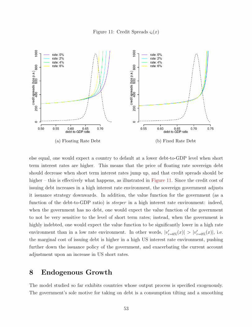
Figure 11: Credit Spreads ςi(x)

(a) Floating Rate Debt (b) Fixed Rate Debt

else equal, one would expect a country to default at a lower debt-to-GDP level when short

term interest rates are higher. This means that the price of floating rate sovereign debt

should decrease when short term interest rates jump up, and that credit spreads should be

higher – this is effectively what happens, as illustrated in Figure 11. Since the credit cost of

issuing debt increases in a high interest rate environment, the sovereign government adjusts

it issuance strategy downwards. In addition, the value function for the government (as a

function of the debt-to-GDP ratio) is steeper in a high interest rate environment: indeed,

when the government has no debt, one would expect the value function of the government

to not be very sensitive to the level of short term rates; instead, when the government is

highly indebted, one would expect the value function to be significantly lower in a high rate

environment than in a low rate environment. In other words, |v′r=6%(x)| > |v′r=0%(x)|, i.e.

the marginal cost of issuing debt is higher in a high US interest rate environment, pushing

further down the issuance policy of the government, and exacerbating the current account

adjustment upon an increase in US short rates.

8 Endogenous Growth

The model studied so far exhibits countries whose output process is specified exogenously.

The government’s sole motive for taking on debt is a consumption tilting and a smoothing

53

motive. What happens when the government instead borrows from external creditors in order

to finance domestic investments and capital accumulation? This section answers this ques-

tion, and emphasizes two sources of debt overhang channels through which highly indebted

sovereign government’s capital investment decisions might be distorted. This enhanced model

provides a simple micro-foundation to the output process of Aguiar and Gopinath (2004),

Aguiar and Gopinath (2006), and many other articles in the sovereign debt literature, in

which output growth is a mean-reverting variable.

Assume now that the country n has a production technology Yt = aKt, with a > 0,

where Kt is the number of effective units of capital in the small open economy. Assume that

effective capital evolves according to:

dKt = (Ht − ηKt)dt+Ktσ · dBt (40)

Ht represents effective capital investments and η is the rate of depreciation of capital. The

effective capital in this economy is hit by capital quality shocks similar to those in standard

continuous time macro models such as Brunnermeier and Sannikov (2014) or He and Kr-

ishnamurthy (2014). Capital investments come with adjustment costs equal to G(Ht, Kt) =

g(Ht/Kt)Kt, with g strictly convex, g(0) = g′(0) = 0. For simplicity, I will assume that

g(h) = ψ2h2, where h is the investment rate per unit of effective capital. Government debt

dynamics continue to follow equation (7). The government’s resource constraint can now be

written:

Ct +Ht = aKt + ItDt − (κ+m)Ft −G(Ht, Kt) (41)

Equation (41) simply says that the sum of consumption Ct and investment Ht need to be

equal to the sum of output aKt and capital markets net flows ItDt − (κ + m)Ft, net of

investment adjustment costs G(Ht, Kt). If and when the government elects to default, its

(efficiency units of) capital stock suffers a discrete drop, falling from Kτ− to Kτ = αKτ−.

The government is also excluded from capital markets for an exponentially distributed time

period, and exits autarky with a debt-to-capital ratio that is θ times its debt-to-capital ratio

pre-default.

The strategy of the government now consists in choosing an issuance policy I, an invest-

ment policy H , and a default policy τ in order to maximize its objective function. The debt

price follows equations (12) and (13). I look for an equilibrium where the debt-to-capital ratio

xt := Ft/Kt and the SDF regime st are the state variables of this modified environment. The

details of the equilibrium calculations are displayed in Section A.1.19. When the debt-to-

capital ratio of the country is x and when the SDF state is i, the debt price is equal to Di(x)

and the life-time utility function for the government is equal to vi(x)K1−γ. The optimal debt

54

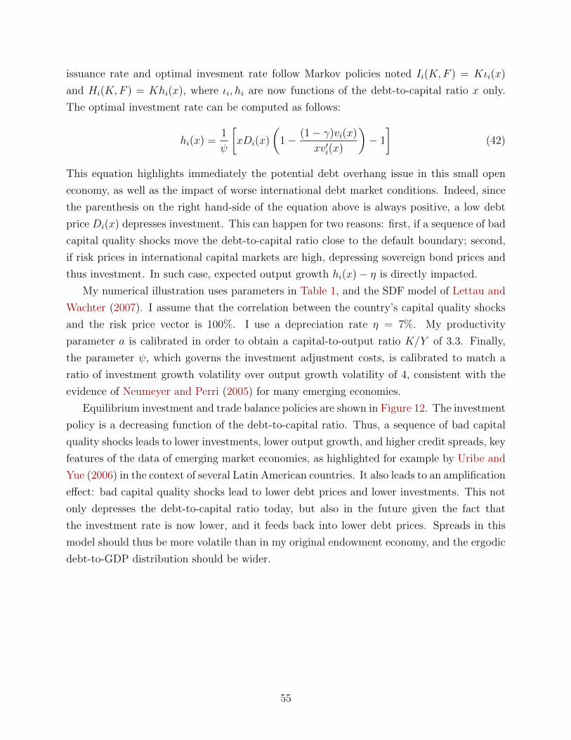
issuance rate and optimal invesment rate follow Markov policies noted Ii(K,F ) = Kιi(x)

and Hi(K,F ) = Khi(x), where ιi, hi are now functions of the debt-to-capital ratio x only.

The optimal investment rate can be computed as follows:

hi(x) =1

ψ

[xDi(x)

(1− (1− γ)vi(x)

xv′i(x)

)− 1

](42)

This equation highlights immediately the potential debt overhang issue in this small open

economy, as well as the impact of worse international debt market conditions. Indeed, since

the parenthesis on the right hand-side of the equation above is always positive, a low debt

price Di(x) depresses investment. This can happen for two reasons: first, if a sequence of bad

capital quality shocks move the debt-to-capital ratio close to the default boundary; second,

if risk prices in international capital markets are high, depressing sovereign bond prices and

thus investment. In such case, expected output growth hi(x)− η is directly impacted.

My numerical illustration uses parameters in Table 1, and the SDF model of Lettau and

Wachter (2007). I assume that the correlation between the country’s capital quality shocks

and the risk price vector is 100%. I use a depreciation rate η = 7%. My productivity

parameter a is calibrated in order to obtain a capital-to-output ratio K/Y of 3.3. Finally,

the parameter ψ, which governs the investment adjustment costs, is calibrated to match a

ratio of investment growth volatility over output growth volatility of 4, consistent with the

evidence of Neumeyer and Perri (2005) for many emerging economies.

Equilibrium investment and trade balance policies are shown in Figure 12. The investment

policy is a decreasing function of the debt-to-capital ratio. Thus, a sequence of bad capital

quality shocks leads to lower investments, lower output growth, and higher credit spreads, key

features of the data of emerging market economies, as highlighted for example by Uribe and

Yue (2006) in the context of several Latin American countries. It also leads to an amplification

effect: bad capital quality shocks lead to lower debt prices and lower investments. This not

only depresses the debt-to-capital ratio today, but also in the future given the fact that

the investment rate is now lower, and it feeds back into lower debt prices. Spreads in this

model should thus be more volatile than in my original endowment economy, and the ergodic

debt-to-GDP distribution should be wider.

55

Figure 12: Endogenous Growth – Policies

(a) Investment policy hi(x) (b) Trade balance 1− ci(x)

9 Conclusion

In this paper, I develop a new modeling framework to study sovereign debt quantities and

prices by leveraging continuous time technology. This tractable approach leads to semi-closed

form expressions for key asset pricing moments of interest, which enables me to discuss char-

acteristics of the stochastic discount factor that are needed to explain properties of sovereign

spreads, sovereign debt returns and cross-country spread correlations. The approach I pro-

pose reduces significantly the number of state variables typically present in discrete time

sovereign debt models and opens the door to partial model estimation. My quantitative

application shows that this modeling framework has the ability to match many quantities

and price moments of the data, but fails on two dimensions: (i) the model-implied dispersion

of the debt-to-GDP ergodic distribution remains an order of magnitude smaller than in the

data, and (ii) the magnitude of excess returns on sovereign debt requires very high levels of

correlation between countries’ output processes and SDFs typically used in the asset pric-

ing literature to explain properties of US equity market returns – if the creditors’ SDF is

associated with US consumption or output dynamics, the empirical correlation between the

US GDP and the GDP of my countries of interest is too low compared to the model esti-

mates required to rationalize this high level of expected excess returns. My framework can

be extended in multiple directions without adding any complexity or state variable. I show

56

for example how to layer a linear production technology and study capital accumulation and

the impact of debt overhang on investment decisions. One can also analyze an environment

with exogenously specified sudden stops, by adding discrete SDF states where the sovereign

government is prevented from issuing any debt. Finally, more theoretical work needs to be

done, for example by leveraging viscosity theory and existence results for nested ordinary

differential equations, in order to establish the existence of a Markov perfect equilibrium of

the game between the sovereign government and its creditors.

57

References

Aguiar, Mark and Manuel Amador. 2013. “Take the Short Route: How to repay and restruc-

ture sovereign debt with multiple maturities.” Tech. rep., National Bureau of Economic

Research.

Aguiar, Mark, Satyajit Chatterjee, Harold L Cole, and Zachary Stangebye. 2016a. “Belief

Regimes and Sovereign Debt Crises.” .

———. 2016b. “Quantitative Models of Sovereign Debt Crises.” Available at SSRN 2746808

.

Aguiar, Mark and Gita Gopinath. 2004. “Emerging market business cycles: The cycle is the

trend.” Tech. rep., National Bureau of Economic Research.

———. 2006. “Defaultable debt, interest rates and the current account.” Journal of inter-

national Economics 69 (1):64–83.

Arellano, Cristina. 2008. “Default risk and income fluctuations in emerging economies.” The

American Economic Review :690–712.

Arellano, Cristina and Ananth Ramanarayanan. 2012. “Default and the maturity structure

in sovereign bonds.” Journal of Political Economy 120 (2):187–232.

Benjamin, David and Mark LJ Wright. 2009. “Recovery before redemption: A theory of

delays in sovereign debt renegotiations.” Available at SSRN 1392539 .

Borri, Nicola and Adrien Verdelhan. 2011. “Sovereign risk premia.” In AFA 2010 Atlanta

Meetings Paper.

Broner, Fernando A, Guido Lorenzoni, and Sergio L Schmukler. 2013. “Why do emerging

economies borrow short term?” Journal of the European Economic Association 11 (s1):67–

100.

Brunnermeier, Markus K and Yuliy Sannikov. 2014. “A macroeconomic model with a financial

sector.” The American Economic Review 104 (2):379–421.

Bulow, Jeremy, Kenneth Rogoff, and Rudiger Dornbusch. 1988. “The buyback boondoggle.”

Brookings Papers on Economic Activity 1988 (2):675–704.

Chatterjee, Satyajit and Burcu Eyigungor. 2015. “A seniority arrangement for sovereign

debt.” .

58

Chen, Hui. 2010. “Macroeconomic conditions and the puzzles of credit spreads and capital

structure.” The Journal of Finance 65 (6):2171–2212.

Cline, William R et al. 1995. “International debt reexamined.” Peterson Institute Press: All

Books .

Coase, Ronald H. 1972. “Durability and monopoly.” The Journal of Law & Economics

15 (1):143–149.

Cole, Harold L and Timothy J Kehoe. 1996. “A self-fulfilling model of Mexico’s 1994–1995

debt crisis.” Journal of international Economics 41 (3):309–330.

DeMarzo, Peter and Zhiguo He. 2014. “Leverage dynamics without commitment.” Tech.

rep., Working Paper.

Dooley, Michael P. 1994. “A retrospective on the debt crisis.” Tech. rep., National Bureau

of Economic Research.

Duffie, Darrell and Costis Skiadas. 1994. “Continuous-time security pricing: A utility gradient

approach.” Journal of Mathematical Economics 23 (2):107–131.

Eaton, Jonathan and Mark Gersovitz. 1981. “Debt with potential repudiation: Theoretical

and empirical analysis.” The Review of Economic Studies 48 (2):289–309.

Gordin, Mikhail I. 1969. “Central limit theorem for stationary processes.” Doklady Akademii

Nauk SSSR 188 (4):739.

Gul, Faruk, Hugo Sonnenschein, and Robert Wilson. 1986. “Foundations of dynamic

monopoly and the Coase conjecture.” Journal of Economic Theory 39 (1):155–190.

Hansen, Lars P and Ravi Jagannathan. 1990. “Implications of security market data for

models of dynamic economies.”

Hansen, Lars Peter. 2012a. “Dynamic valuation decomposition within stochastic economies.”

Econometrica 80 (3):911–967.

———. 2012b. “Risk pricing over alternative investment horizons.” Becker Friedman Insti-

tute for Research in Economics Working Paper (2012-008).

Hatchondo, Juan Carlos and Leonardo Martinez. 2009. “Long-duration bonds and sovereign

defaults.” Journal of International Economics 79 (1):117–125.

59

He, Zhiguo and Arvind Krishnamurthy. 2014. “A macroeconomic framework for quantifying

systemic risk.” Tech. rep., National Bureau of Economic Research.

Hebert, Benjamin and Jesse Schreger. 2016. “The Costs of Sovereign Default: Evidence from

Argentina.” Tech. rep., National Bureau of Economic Research.

Kahn, Charles. 1986. “The durable goods monopolist and consistency with increasing costs.”

Econometrica: Journal of the Econometric Society :275–294.

Kushner, Harold J and Paul Dupuis. 2001. Numerical methods for stochastic control problems

in continuous time, vol. 24. Springer.

Lee, Bong-Soo and Beth Fisher Ingram. 1991. “Simulation estimation of time-series models.”

Journal of Econometrics 47 (2-3):197–205.

Leland, Hayne E. 1994. “Corporate debt value, bond covenants, and optimal capital struc-

ture.” The journal of finance 49 (4):1213–1252.

———. 1998. “Agency Costs, Risk Management, and Capital Structure (Digest Summary).”

Journal of finance 53 (4):1213–43.

Lettau, Martin and Jessica A Wachter. 2007. “Why is long-horizon equity less risky? a

duration-based explanation of the value premium.” The Journal of Finance 62 (1):55–92.

Lizarazo, Sandra Valentina. 2013. “Default risk and risk averse international investors.”

Journal of International Economics 89 (2):317–330.

Longstaff, Francis A, Jun Pan, Lasse H Pedersen, and Kenneth J Singleton. 2007. “How

sovereign is sovereign credit risk?” Tech. rep., National Bureau of Economic Research.

———. 2011. “How sovereign is sovereign credit risk?” American Economic Journal:

Macroeconomics 3 (2):75–103.

Maskin, Eric and Jean Tirole. 2001. “Markov perfect equilibrium: I. Observable actions.”

Journal of Economic Theory 100 (2):191–219.

Mendoza, Enrique G. 2002. “Credit, prices, and crashes: Business cycles with a sudden

stop.” In Preventing currency crises in Emerging markets. University of Chicago Press,

335–392.

———. 2010. “Sudden stops, financial crises, and leverage.” The American Economic Review

100 (5):1941–1966.

60

Neumeyer, Pablo A and Fabrizio Perri. 2005. “Business cycles in emerging economies: the

role of interest rates.” Journal of monetary Economics 52 (2):345–380.

Newey, Whitney K and Kenneth D West. 1986. “A simple, positive semi-definite, het-

eroskedasticity and autocorrelationconsistent covariance matrix.”

Nuno, Galo and Carlos Thomas. 2015. “Monetary Policy and Sovereign Debt Vulnerability.”

Tech. rep., mimeo.

Pan, Jun and Kenneth J Singleton. 2008. “Default and recovery implicit in the term structure

of sovereign CDS spreads.” The Journal of Finance 63 (5):2345–2384.

Protter, Philip E. 2005. Stochastic Differential Equations. Springer.

Rose, Andrew K. 2005. “One reason countries pay their debts: renegotiation and international

trade.” Journal of development economics 77 (1):189–206.

Seoane, Hernan D. 2013. “Time-varying volatility, default and the sovereign risk premium.”

Stokey, Nancy L. 1981. “Rational expectations and durable goods pricing.” The Bell Journal

of Economics :112–128.

Tanaka, Ken’ichiro and Alexis Akira Toda. 2015. “Discretizing distributions with exact

moments: Error estimate and convergence analysis.” SIAM Journal on Numerical Analysis

53 (5):2158–2177.

Tanaka, Kenichiro and Alexis Akira Toda. 2013. “Discrete approximations of continuous

distributions by maximum entropy.” Economics Letters 118 (3):445–450.

Tauchen, George. 1986. “Finite state markov-chain approximations to univariate and vector

autoregressions.” Economics letters 20 (2):177–181.

Tauchen, George and Robert Hussey. 1991. “Quadrature-based methods for obtaining ap-

proximate solutions to nonlinear asset pricing models.” Econometrica: Journal of the

Econometric Society :371–396.

Tomz, Michael and Mark LJ Wright. 2013. “Empirical research on sovereign debt and de-

fault.” Tech. rep., National Bureau of Economic Research.

Uribe, Martin and Vivian Z Yue. 2006. “Country spreads and emerging countries: Who

drives whom?” Journal of international Economics 69 (1):6–36.

61

A Appendix

A.1 Proofs and Detailed Calculations

A.1.1 A Useful Discrete Time Limit

In this section, I study a discrete time counterpart to the continuous-time model developed

in this paper. ∆t will represent a small time interval. I study the limit of a simple sovereign

default model as ∆t → 0, and show heuristically that no short term debt can be supported

in equilibrium at such limit. I focus on a government that has iso-elastic time-separable

preferences with rate of time preference δ and risk-aversion γ as follows:

E

[∞∑i=0

e−δi∆tC1−γi∆t

1− γ∆t|F0

]

Government output follows the discrete time equivalent of a geometric Brownian motion:

Y(i+1)∆t

Yi∆t= eω(i+1)∆t

In the above, ω(i+1)∆t is an F(i+1)∆t measurable binomial random variable that can take values

+σ√

∆t or −σ√

∆t with respective probabilities pu and pd:

pu :=1

2

(1 +

(µ− 1

2σ2)√

∆t

σ

); pd :=

1

2

(1−

(µ− 1

2σ2)√

∆t

σ

)

Thus, ω(i+1)∆ti≥0 is a sequence of i.i.d. random variables, and I will use ω∆t for simplicity

to denote one of these random variables. When ∆t→ 0, I have the following limits:

E [eω∆t ] = 1 + µ∆t+ o (∆t)

var [eω∆t ] = σ2∆t+ o (∆t)

The government has one-period debt at its disposal. Let Bi∆t be the stock of debt that

the government has to repay at time i∆t. Let D(B(i+1)∆t, Yi∆t

)be the price of one unit of

debt if the government plans to issue, at date i∆t, B(i+1)∆t units of debt maturing at period

(i+ 1)∆t. The government resource constraint at time i∆t is as follows:

Ci∆t∆t = Yi∆t∆t−Bi∆t +D(B(i+1)∆t, Yi∆t

)B(i+1)∆t

62

Upon default, GDP suffers a permanent shock of size 1 − α and the government is in au-

tarky forever after. Thus, if the pre-default output value is Yi∆t, the value function for the

government in default is equal to Vd(Yi∆t), which satisfies:

Vd(Y ) =(αY )1−γ

1− γ∆t+ e−δ∆tE [Vd (eω∆tY )]

Guessing that Vd(Y ) = vdY1−γ, the constant vd is equal to:

vd =

α1−γ

1−γ ∆t

1− e−δ∆tE [e(1−γ)ω∆t ]=

α1−γ

1−γ

δ + (γ − 1)(µ− 1

2γσ2) + o(1)

The latter equality is valid when ∆t→ 0. The government problem is as follows:

V0 (B, Y ) = max (Vc (B, Y ) , Vd (Y ))

Vd (Y ) = vdY1−γ

Vc (B, Y ) = maxB′

[(Y + 1

∆t(D (B′, Y )B′ −B)

)1−γ∆t

1− γ+ e−δ∆tE [V0 (B′, Y ′) |Y ]

]

The bond price verifies D(B′, Y ) = e−r∆t Pr (Vc (B′, Y ′) ≥ Vd(Y′)|Y ), where r is the interest

rate at which lenders discount risk-free cashflows. This formula assumes that upon default,

sovereign creditors recover nothing from their defaulted debt claim. One can show that for

any bond price function that is homogeneous of degree zero and decreasing in B′, the value

function Vc is homogeneous of degree 1−γ and the best “default” response by the government

is to follow a linear barrier policy of the form τ := inft : Bt ≥ xYt for some endogenously

determined constant x (which depends on the time step ∆t)22. Noting x := B/Y , and

using the homogeneity property of the value function, the government life-time utility can

be written Vc(B, Y ) = vc(x)Y 1−γ, and the government problem can be simplified as follows:

vc (x) = maxx′

[(1 + 1

∆t(D (x′)x′ − x)

)1−γ∆t

1− γ+ e−δ∆tE

[e(1−γ)ω∆t max

(vd, vc

(e−ω∆tx′

))]]

For simplicity, I assume that the choice set for the debt-to-GDP ratio of the government is

discrete. In other words, I discretize the state space into a grid G∆t consisting of a countable

22Of course this statement is assuming the existence of the value function Vc, which is the fixed point ofa functional equation. Since my discussion on the lack of equilibria with defaultable debt at the limit of mydiscrete time economies is only heuristic, I side-step the proof of existence of Vc.

63

number of points xi = eiσ√

∆t, for i ∈ N, where I note id the default index23. In other words,

I assume that at x = xid , the government strictly prefer defaulting over repaying, while

for i < id, the government weakly prefer repaying over defaulting. This model structure

guarantees that the debt-to-GDP ratio stays on the grid G∆t at all times, irrespective of the

sequence of GDP shocks and decisions made by the government. In any cutoff equilibrium

with default threshold x = xid , the debt price must satisfy:

D(xi) =

e−r∆t if i < id − 1

12

(1 +

(µ− 12σ2)√

∆t

σ

)e−r∆t if i = id − 1

0 if i ≥ id

Now consider the resource constraint for the government if at the beginning of a given period,

x = xi, with i = id − 1. Since i < id, it is optimal for the government to continue to

perform on its debt obligations. If the government selects a debt-to-GDP ratio xj < xi, the

consumption-to-output ratio, using the resource constraint, is equal to:

1 +1

∆t

(ejσ√

∆t−r∆t − eiσ√

∆t)

=(j − i)σ√

∆t+ o

(1√∆t

)→

∆t→0−∞

If the government selects a debt-to-GDP ratio xj = xi, the consumption-to-output ratio is

equal to:

1 +1

∆t

(1

2

(1 +

(µ− 1

2σ2)√

∆t

σ

)eiσ√

∆t−r∆t − eiσ√

∆t

)= − 1

2∆t+ o

(1

∆t

)→

∆t→0−∞

Of course if the government selects a debt-to-GDP ratio xj = xid , it obtains no proceeds from

its debt issuance – this decision cannot be optimal. Thus, as ∆t → 0, the only possibility

for government consumption to be positive at all points of the state space xi < x is for the

default boundary to converge to zero. Note that this conclusion stems from (A) the shape of

the government bond price schedule (at I take ∆t → 0, such debt price schedule converges

to a step function, equal to the risk-free benchmark for x < x and equal to zero at x ≥ x),

and (B) the continuous sample path of geometric Brownian motions. Had the output process

featured jumps, a cutoff equilibrium with strictly positive debt can be supported.

23This model structure implicitly assumes that the government is prevented from saving. This can also beachieved endogenously by using a sufficiently high rate of time preference δ.

64

A.1.2 Output Process in this Article vs. Aguiar and Gopinath (2006)

The output process in Aguiar and Gopinath (2006) can be recast in continuous time as

follows:

Yt = eztΓt

d ln Γt = ln gtdt

dzt = −κz (zt − µz) dt+ σzdBzt

d ln gt = −κg (ln gt − lnµg) dt+ σgdBgt

In the above, Bgt , B

zt are standard Brownian motions assumed to be independent, κz, κg

are positive constants that parametrize the speed of mean reversion of the processes zt and

ln gt respectively. Two approaches can be used to approximate the output process above by

equation (1).

In the first approach, conditional and unconditional moments of consumption growth can

be matched. One can for example match the s-lagged auto-correlation of log consumption

growth Rmodel(s) for both models. Such auto-correlations are equal to:

RAG(s) = e−κgs

RGBM(s) =

∑Nsi=1 πi

(µi − 1

2|σi|2

)∑Nsj=1

[(esΛ)ij− πj

] (µj − 1

2|σj|2

)∑Ns

i=1 πi(µi − 1

2|σi|2

)2 −(∑Ns

i=1 πi(µi − 1

2|σi|2

))2

One can also match the unconditional log consumption growth volatility Σmodel for both

models. Such log consumption growth volatilities are equal to:

ΣAG = σz

ΣGBM =

√√√√ Ns∑i=1

πi|σi|2

In the second approach, one can use a procedure introduced by Gordin (1969) to extract a

martingale component to the logarithm of output for both models, and match separately (a)

the volatility of the martingale component of both models, (b) conditional and unconditional

moments of the stationary component of both models, and (c) the time trend of both models.

For the model of Aguiar and Gopinath (2006), the decomposition of lnYt takes the following

65

form:

d lnYt =σgκgdBg

t − d(

1

κgln gt − zt

)+ lnµgdt

lnYt − lnY0 =

∫ t

0

σgκgdBg

s︸ ︷︷ ︸martingale component

+

[1

κgln g0 − z0

]−[

1

κgln gt − zt

]︸ ︷︷ ︸

stationary component

+ t lnµg︸ ︷︷ ︸time trend

Thus, the permanent component to log output is purely driven by (rescaled) shocks to the

state variable ln gt, while the state variable zt has a purely transitory role. The long-run

time trend in log-output is equal to lnµg. When I focus on the output process driven by

equation (1) (and assuming, for the purpose of this section, that Bt is unidimensional), I can

compute small increments in logarithms as follows:

d lnYt =

(µst −

1

2σ2st

)dt+ σstdBt

In the above, st is the discrete state Markov chain with generator matrix Λ and stationary

density π. In such case, note that:

E [d lnYt|Ft] =

(µst −

1

2σ2st

)dt

Let κ2,t :=∫ toσsudBu and note that for τ > t, E [κ2,τ |Ft] = κ2,t, in other words κ2,t is a

martingale. I then compute the long term average of log output growth:

ln g∞ : = π ·(µ− 1

2σ2

)I create the function f (s) := µs − 1

2σ2s − ln g∞ =

(µ− 1

2σ2 − ln g∞1

)· est , es is an Ns × 1

column vector with entry s equal to 1, and all other entries equal to zero, and compute:∫ ∞0

E [f (st+u) |Ft] du = Λ−1

(µ− 1

2σ2 − ln g∞1

)· est

In the above, Λ−1 is the generalized inverse of the generator matrix Λ (since the rows of the

matrix Λ sum up to zero, Λ is not invertible). Finally, I introduce the martingale κ1,t, defined

as follows:

κ1,t :=

∫ t

0

Ns∑i=1

Λ−1

(µ− 1

2σ2 − ln g∞1

)·(ei − esu−

)dN (su−,i)

u +

∫ t

0

(µ− 1

2σ2 − ln g∞1

)· esudu

66

I can then decompose increments in log output growth as follows:

d lnYt = d (κ1,t + κ2,t)− Λ−1

(µ− 1

2σ2 − ln g∞1

)·(est − est−

)dN

(st−,st)t + ln g∞dt

lnYt − lnY0 =

∫ t

0

d (κ1,s + κ2,s)︸ ︷︷ ︸martingale component

+ Λ−1

(µ− 1

2σ2 − ln g∞1

)· (es0 − est)︸ ︷︷ ︸

stationary component

+ t ln g∞︸ ︷︷ ︸time trend

Thus, in the case of this article, the martingale component of log output is the sum of a

Brownian process κ1,t and a jump process κ2,t, while the stationary component is a pure

jump process. By carefully parameterizing µ,σ,Λ, one can approximate the long run trend,

stationary and martingale components in Aguiar and Gopinath (2006) by a stochastic process

that follows equation (1).

A.1.3 No-Debt Life-Time Utility

I note Ji (Y ) the life-time utility value when the government cannot issue debt, when the

level of output is Y and when the Markov state is st = i. I postulate that this life-time utility

can be written Ji(Y ) = KiY1−γ for some constants Kii≤Ns to be determined. Ji verifies

the following HJB equation:

0 = ϕ (Yt, Jst(Yt)) +AJst(Yt)

For convenience, I have introduced the differential operator A, defined for any stochastic

process Ztt≥0 (belonging to an appropriate class of stochastic processes) as follows:

AZt := limε→0

E [Zt+ε|Ft]− Ztε

(43)

Injecting my guess function for Ji, I obtain the following equation, for i ≤ Ns:

0 = δ1− γ1− ρ

KiY1−γ

(1

[(1− γ)Ki]1−ρ1−γ− 1

)+ µi(1− γ)KiY

1−γ − 1

2γ(1− γ)|σi|2KiY

1−γ +Ns∑j=1

ΛijKjY1−γ

Dividing by KiY1−γ and simplifying, the set of constants K := Kii≤Ns must satisfy:[

diagi(Ai)−1− ρ1− γ

Λ

][(1− γ)K] = δ [(1− γ)K]

ρ−γ1−γ

67

Vector exponentiation in the equation above has to be understood element by element. Under

assumption 1, this set of Ns equations in Ns unknown has a unique solution.

A.1.4 Creditors’ Stochastic Discount Factor

The discussion below is substantially similar to the discussion in Chen (2010). Assume

a representative creditor whose equilibrium consumption Cc,t follows, under the physical

measure P:

dCc,tCc,t

= µc,stdt+ σc,st · dBt

In the above, stt≥0 follows a discrete state Markov process with generator matrix Λ =

(Λij)1≤i,j≤Ns . Ns is the total number of discrete states. Assume that such creditor ranks

consumption streams according to the utility specification:

Ut = E[∫ +∞

t

Ψ (Cs, Us) ds|Ft]

(44)

In the above, the aggregator Ψ is assumed to be equal to:

Ψ (C,U) := δc1− γc1− ρc

U

(C1−ρc

((1− γc)U)1−ρc1−γc

− 1

)

The representative creditor’s life-time utility function can be written Ut =(hstYt)

1−γ

1−γ , where

the constants hi1≤i≤Ns satisfy the set of non-linear equations:

0 = δc1− γc1− ρc

hρc−1i + (1− γc)µc,i −

1

2γc(1− γc)|σc,i|2 − δc

1− γc1− ρc

+Ns∑j=1

Λij

(hjhi

)1−γc

As Duffie and Skiadas (1994) shows, the marginal utility process associated with recursive

preferences can be written:

Mt = exp

[∫ t

0

∂Ψ

∂U(Cc,z, Uc,z) dz

]∂Ψ

∂C(Cc,t, Uc,t) (45)

Applying Ito’s lemma then leads to the following dynamic evolution of Mt:

dMt

Mt

= −rstdt− νst · dBt +∑st 6=st−

(eυ(st−,st) − 1

) (dN

(st−,st)t − Λst−,stdt

)(46)

68

In the above, N(st−,st)t is a Poisson counting process for transitions from state st− to state st.

For each discrete Markov state i, the state dependent risk price vector νi is equal to:

νi = γcσc,i (47)

For each discrete Markov state i, the state dependent risk free rate ri is equal to:

ri = −δc1− γc1− ρc

[(ρc − γc1− γc

)hρc−1i − 1

]+ γcµc,i −

1

2γc(1 + γc)|σc,i|2 −

Ns∑j=1

Λijeυ(i,j) (48)

Finally, the SDF relative jump sizes encoded via υ(i, j) are equal to:

υ(i, j) = (ρc − γc) ln

(hjhi

)(49)

Compensations per unit of Brownian risk can be read via the coordinates of the vector νst ,

while jump compensation is encoded via eυ(st−,st)−1. Indeed, take any asset whose valuation

Vt follows:

dVtVt

= µv,tdt+ σv,t · dBt +∑st 6=st−

(eξv(st−,st) − 1

) (dN

(st−,st)t − Λst−,stdt

)Absence of arbitrage imposes that MtVt be a local martingale, in other words E [d (MtVt)] = 0.

Using Ito’s lemma leads to the following pricing restriction:

µv,t − rst = σv,t · νst −∑st 6=st−

(eξv(st−,st) − 1

) (eυ(st−,st) − 1

)Λst−,st

For example, a claim to the creditor’s aggregate consumption Cc,t = Yc,t has a price Pc,t =

Pc,st(Yt) that solve the following HJB equation:

riPc,i(Y ) = Y + (µc,i − νi · σc,i)Y P ′c,i(Y ) +1

2|σc,i|2Y 2P ′′c,i(Y ) +

Ns∑j=1

ΛijPc,j(Y )

The solution to the system above is of the form Pc,i(Y ) = Pc,iY , for a set of constants

Pc,ii≤Ns that are equal to:

Pc =[diagi (ri + νi · σc,i − µc,i)− Λ

]−1

1 (50)

69

Expected excess returns on this claim thus take the following form:

E[d (Pc,stYt) + Ytdt

Pc,stYt− rstdt|Ft

]= νst · σc,stdt−

∑s′

Λst−s′

(Pc,s′

Pc,st−− 1

)(eυ(st−,s′) − 1

)dt

A.1.5 A General Equilibrium Interpretation

In this section, I describe how to obtain, in a general equilibrium setting, the stochastic

discount factor Mt, whose dynamics are given by equation (10). For this, I introduce the

subscript “n” for a country’s identity, and assume a continuum of countries of measure 1. Y nt

is re-interpreted as tax collections of country n – imagine for example that country n has a

flow output Xnt and a tax rate εn, such that Y n

t = εnXnt . Suppose country n’s output evolves

as follows:

dXnt

Xnt

= µstdt+ σst · dBt + σndBnt

Bnt is a country-specific Brownian shock that is independent of Bt, the vector of aggregate

Brownian shocks. Note that all countries need to have the same expected growth rate µst in

all states st, but not necessarily the same output volatility24. The dynamics for aggregate

world output is thus:

dXt =

∫dXn

t dn

=

∫[µstX

nt dt+Xn

t (σst · dBt + σndBnt )] dn

= Xt (µstdt+ σst · dBt)

The latter equality uses the law of large numbers and leverages the fact that Xnt and dBn

t are

not correlated. Given that tax revenues of country n are equal to Y nt = εnXn

t , the government

revenue process Y nt follows the same stochastic differential equation as Xn

t . Government n

resource constraint is the following:

Cnt = Y n

t + Int Dnt − (κ+m)F n

t

Cnt represents government spending, Int represents government debt issuances (debt is issued

at priceDnt ), and F n

t represents the face value of government debt. We assume for the moment

that εn is fixed and exogenous, and that the government will only choose its financing and

24Forcing all countries to have the same expected GDP growth rate also guarantees that countries all“survive” as t→ +∞, in other words no country becomes arbitrarily small asymptotically.

70

default policies. Due to institutional frictions, government n’s utility function is not exactly

equal to the utility function of its citizens; more specifically, the government maximizes the

following objective function (subject to government resource constraint above):

Jnt = E[∫ +∞

t

ϕ (Cns , J

ns ) ds|Ft

]In other words, the government maximizes flow utility over government spending only; more-

over, the government will be more impatient than its citizens: δ, the rate of time preference

of the government, will verify δ > δc, where δc will be the rate of time preference of the

citizens/creditors (to be discussed shortly). Government of country n may elect to default on

its debt. In such case, the government is shut down from capital markets for some exponen-

tially distributed time (parametrized by λ), and suffers a temporary drop in tax collection

efficiency: while in autarky, the government only collects Y nt = αεnXn

t from its citizens, with

α < 1. Upon exit from financial autarky, the government from country n emerges with a

lower debt burden, and recovers its pre-default tax efficiency Y nt = εnXn

t . Note that the drop

in tax collections suffered by the defaulting government is only temporary, and lasts the time

of the capital market’s exclusion.

Government debt is bought by a “representative world investor” – in other words, a citizen

whose equilibrium consumption process is proportional to world consumption. Let Dt be the

set of indices of countries in default at time t, and Dct = [0, 1]\Dt its complement. Remember

that world citizens enjoy flow consumption Γt equal to:

Γt :=

∫n∈Dct

[(1− εn)Xnt + (κ+m)F n

t − Int Dnt ] dn+

∫n∈Dt

(1− αεn)Xnt dn = Xt − Ct

In the above, Ct represents aggregate government spending. Consumption by the “represen-

tative world investor” is simply equal to world output minus taxes paid plus income received

on its government debt portfolio minus investments in government debt. Assume this “rep-

resentative world investor” faces dynamically complete markets, and has preferences over

consumption Γt and government spending Ct as follows:

Ut = E[∫ +∞

t

Ψ (Γs + Cs, Us) ds|Ft]

In other words, consumption and government spending are perfect substitutes in the rep-

resentative investor’s preferences. Given those assumptions, the investor’s equilibrium con-

sumption (via market clearing) is equal to Γt + Ct = Xt, and the investor’s marginal utility

71

is given by equation (45), meaning that the pricing kernel Mt evolves as follows:

dMt

Mt

= −rstdt− νst · dBt +∑st 6=st−

(eυ(st−,st) − 1

) (dN

(st−,st)t − Λst−,stdt

)rs, νs and the SDF jumps υ(s, s′) correspond to those described in Section A.1.4.

A.1.6 Controlled Stochastic Processes Y(τ )t and F

(I,τ )t

An admissible issuance policy Itt≥0 of the government is a progressively measurable process

that is a function of the payoff-relevant variables. In other words, It = Ist(Yt, Ft), for a set

of measurable functions I := Iii≤Ns . I will require the function It to satisfy the standard

integrability condition, for all t ≥ 0, almost surely:

E[∫ t

0

|Is|ds]< +∞

An admissible default policy is an increasing sequence of stopping times (with respect to Ft)noted τ = τkk≥1, which can be written (for k ≥ 0), τk+1 = inft ≥ τk+τe,k : (Yt, Ft) ∈ Ost,for a finite number of Borel sets Oii≤Ns , where τe,kk≥1 is a sequence of i.i.d. exponentially

distributed times (with parameter λ), and where I have set τ0 = τe,0 = 0.

For a given admissible default policy τ ∈ T , define N(τ )d,t := maxk ∈ N : τk ≤ t (resp.

N(τ )e,t := maxk ∈ N : τk + τe,k ≤ t) to be the counting process for default events (resp.

capital markets re-entry events). Let 1(τ )d,t be the default indicator, equal to 1 when the

sovereign government is in default, and zero otherwise:

1(τ )d,t := 1t∈[τNd,t ,τNd,t+τe,Nd,t)

Using this notation, the dynamic evolution of the controlled stochastic process Y(τ )t can be

expressed as follows:

dY(τ )t = Y

(τ )t−

(µstdt+ σst · dBt + (α− 1)dN

(τ )d,t

)(51)

Similarly, the dynamic evolution of the controlled stochastic process F (I,τ ) can be expressed

72

as follows:

dF(I,τ )t =

(It− −mF (I,τ )

t−

)(1− 1

(τ )d,t

)dt

+

(θα exp

[∫ t

τNd,t

(µsu −

1

2|σsu |2

)du+ σsu · dBu

]− 1

)F

(I,τ )t− dN

(τ )e,t (52)

The drift term in the dynamic evolution of F(I,τ )t relates to issuances and debt redemptions

when the government is performing under its debt obligations, while the jump term relates to

reductions in the debt face value in connection with a restructuring and re-entry into capital

markets post-default.

Given a debt price schedule D := Di(·, ·)i≤Ns that the government faces, and given

admissible issuance and default policies (I, τ ) used by the government (where (I, τ ) might

not necessarily be consistent with the debt prices D), there is a controlled flow consumption

process C(I,τ ;D)t :

C(I,τ ;D)t =

[Y

(τ )t + ItDst

(Y

(τ )t , F

(I,τ )t

)− (κ+m)F

(I,τ )t

] (1− 1

(τ )d,t

)+ Y

(τ )t 1

(τ )d,t

The indicator functions in this expression highlight the fact that the government can smooth

consumption via debt issuances and buy-backs when performing, while it is unable to do so

in default.

A.1.7 Monotonicity of Vi

Take a set of debt price functions Di (·, ·)i≤Ns that are homogeneous of degree zero and

decreasing in F . I focus my attention on two initial levels of output, Y (1) and Y (2) > Y (1),

and show that I must have Vi(Y(1), F ;D) < Vi(Y

(2), F ;D). First, take any arbitrary policy

(I, τ ) ∈ I ×T (not necessarily optimal) followed by the government. Following the issuance

policy I and starting in state (Y (2), F ) yields strictly higher flow payoffs at each time t.

Indeed, Y (τ )t |Y0 = Y (2) is almost surely greater than Y (τ )

t |Y0 = Y (1). In addition,

ItDst

(Y

(τ )t , F

(I,τ )t

)|Y0 = Y (2) is almost surely greater than ItDst

(Y

(τ )t , F

(I,τ )t

)|Y0 =

Y (1), since the debt price conditioned on starting in state (Y (2), F ) is almost surely greater

than the debt price conditioned on starting in state (Y (1), F ) (since I assumed that the debt

price is decreasing in the debt face value). Thus, C(I,τ ;D)t |Y0 = Y (2) is almost surely

greater than C(I,τ ;D)t |Y0 = Y (1), which means that the life-time utility is increasing in

Y , for any arbitrary issuance and default policy. Thus, the supremum over all feasible

issuance and default policies, Vi (·, ·;D), is also increasing in output Y . The proof for the

monotonicity of Vi (·, ·;D) in F is identical, since consumption C(I,τ ;D)t is decreasing in the

73

level of indebtedness F and since Di(·, ·) is decreasing in F .

I then show that the optimal issuance policy is homogeneous of degree 1 and the optimal

default policy is barrier type. Take an arbitrary (Y, F ), and the related optimal Markov

issuance and default policies (I∗Y,F , τ∗Y,F ) = arg max Ji (Y, F ; (I, τ );D). Take ε > 0, and

focus on starting output and face value levels (εY, εF ). Consider the policy (IεY,εF , τεY,εF ),

such that IεY,εF = εI∗Y,F , and τεY,εF = τ ∗Y,F . Since (I∗Y,F , τ

∗Y,F ) is feasible conditioning on

(Y0, F0) = (Y, F ), since the output dynamics are linear in Y and since the debt face value

dynamics are homogeneous of degree 1 in (Y, F ), it must be the case that (IεY,εF , τεY,εF ) is

feasible conditioning on (Y0, F0) = (εY, εF ). Thus, I have:

Ji(εY, εF ; (IεY,εF , τεY,εF );D) ≤ Vi(εY, εF ;D)

Then assume for a second that the inequality above is strict. If that was the case, then take

(I∗εY,εF , τ∗εY,εF ) = arg max Ji (εY, εF ; (I, τ );D). Consider the policy (IY,F , τY,F ), such that

IY,F = I∗εY,εF /ε, and τY,F = τ ∗εY,εF . Then is it immediate to see that this policy is feasible

conditioned on starting at (Y0, F0), and it is also immediate to see that:

Ji(Y, F ; (IY,F , τY,F );D) > Ji(Y, F ; (I∗Y,F , τ∗Y,F );D) = Vi(Y, F ;D)

This is a contradiction. Thus, the optimal issuance policy is homogeneous of degree 1 in

(Y, F ). Since the value function is decreasing in F and increasing in Y , the default policy

must be a barrier default policy.

A.1.8 Monotonicity of Di

Let (I, τ ) ∈ I × T be admissible issuance and default Markov policies. Assume that I is

homogeneous of degree 1 in (Y, F ) and that τ is barrier. Note Ii(Y, F ) = ιi(F/Y )Y , where

ιi(x) := Ii(1, x), for each Markov state i ≤ Ns. Given these assumptions, the default policy

can be written:

τ = inft ≥ 0 : Ft ≥ Ytxst

= inft ≥ 0 : xt ≥ xst

74

Using Ito’s lemma, xt := Ft/Yt follows the following stochastic differential equation under Q:

dx(ι,τ )t =

(1− 1

(τ )d,t

) [(ιst

(x

(ι,τ )t

)−(m+ µst − |σst |2 − νst · σst

)x

(ι,τ )t

)dt− x(ι,τ )

t σst · dBt

]+ x

(ι,τ )t−

(1

α− 1

)dN

(τ )d,t + x

(ι,τ )t− (θα− 1) dN

(τ )e,t

The debt price is an expected present value of flow payoffs. Since such flow payoffs are

homogeneous of degree zero in (Y, F ), and since the default policy is barrier, the debt

price function must be homogeneous of degree zero. With an abuse of notation, I will note

Di (Y, F ; (ι, τ )) = Di (x; (ι, τ )). Note then that the debt price cannot be greater than the

price Drfi of a risk-free claim to sovereign debt cash-flows, where Drf verifies:

Drf = (κ+m)(

diagi (ri +m)− Λ)−1

1 (53)

I then use a result that will be proven in Section A.1.9: the fact that the defaulted debt price

must satisfy:

Dd(x) = λθαΞ−1D(θx)

The matrix Ns × Ns matrix Ξ is equal to diagi (ri + νi · σi + λ− µi) − Λ. I then introduce

the operator T, defined for any Ns × 1 vector f of continuous decreasing functions whose

ith coordinate is fi : (0,maxj xj) → [0, Drfi ] (Drf

i is the price of risk-free debt is state i, see

equation (53)) as follows. If x ≥ xi, set (Tf)i (x) = λθα [Ξ−1f(θx)]i. If x ≤ xi, then:

(Tf)i (x) : = Ei,x[∫ τ

0

e−∫ t0 (rsu+m)du(κ+m)dt+ λθαe−

∫ τ0 (rsu+m)du

[Ξ−1f(θxτ )

]sτ

](54)

= Drfi + Ei,x

[e−

∫ τ0 (rsu+m)du

(λθα

[Ξ−1f(θxτ )

]sτ−Drf

sτ

)](55)

Given assumption 2, given that θ < 1 and α < 1, and given that the function fi has an image

in [0, Drfi ], it must be the case that λθα [Ξ−1f(·)]i ≤ Drf

i for any state i, which means that

the term in brackets in equation (55) is negative. Thus, (Tf)i (·) is a decreasing function

of x, positive and bounded above by Drfi . The Feynman-Kac theorem also provides for the

continuity of the function (Tf)i (·). Thus, T maps Ns × 1 vectors of continuous bounded

decreasing functions with image in [0, Drfi ] into itself. For any pair of vectors of functions

75

f1,f2 whose components are continuous and decreasing on the interval [0,maxi xi], I have:

| (Tf2 − Tf1)i |(x) = λθαEi,x[e−

∫ τ0 (rsu+m)du

∣∣ [Ξ−1 (f2(θxτ )− f1(θxτ ))]sτ

∣∣]≤ λθα||Ξ−1|| · |f2 − f1|∞

Since λθα||Ξ−1|| < 1 (given assumption 2), T is a contraction, and the contraction map-

ping theorem provides for a unique continuous, bounded and decreasing vector of functions

D(·; (ι, τ )) whose ith component satisfies the functional equation:

Di(x) = Ei,x[∫ τ

0

e−∫ t0 (rsu+m)du(κ+m)dt+ λθαe−

∫ τ0 (rsu+m)du

[Ξ−1D(θxτ )

]sτ

]The function Di is decreasing as required.

A.1.9 Debt Price at Default

I need to compute the debt price in default Ddi (x), for x ≥ xi and 1 ≤ i ≤ Ns. Assume

that at time of default, the state is sτ = i. When the country exits financial autarky, its

debt-to-GDP ratio is equal to Fτ+τe

Yτ+τe= θFτ−

Yτ−= θxτ−. It is possible that xτ > xsτ− when the

sovereign defaults. This happens upon the occurrence of a “jump-to-default”, in other words

a situation where the state jumps from sτ− = j to sτ = i and when xi < xτ− < xj. Thus, I

have the following for x ≥ xi:

Ddi (x) = E

[exp

(−∫ τe

0

rst+udu

)Ft+τeFt−

Dst+τe (θx) |Yt− = Y, st− = i

]= θαE

[exp

(−∫ τe

0

rst+udu

)Yt+τeYt

Dst+τe (θx) |Yt− = Y, st− = i

]In other words, in order to compute Dd

i (x) (for x ≥ xi), I need to solve a system of Ns

equations in Ns unknown Ddj (x)1≤j≤Ns :

rjDdj (x) = (µj − νj · σj)Dd

j (x) + λ(θαDj(θx)−Dd

j (x))

+Ns∑k=1

ΛjkDdk(x)

If I introduce the Ns ×Ns matrix Ξ := diagi (ri + νi · σi + λ− µi)− Λ, and if I note Dd(x)

the Ns × 1 vector with ith element Ddi (x), I obtain:

Dd(x) = λθαΞ−1D(θx)

76

Given assumption 2, the quantity above is well defined and finite. Finally, note that this

equation is valid for each coordinate i for x ≥ xi. Indeed, the model with discrete Markov

states for the SDF generates default waves, via “jumps-to-default” created when the state st

jumps from a state st− = i (for example a state where risk prices are low) to a state st = j

(for example a state where risk prices are high), and when xi > xt > xj. When computing

the full set of functions Di(·)1≤i≤Ns , it is thus essential to compute such function on the

interval [0,maxi xi].

A.1.10 Life-Time Utility HJB Equation

Introduce the probability measure Pr(A) = E[e(1−γ)

∫ t0 σsu ·dBu− 1

2(1−γ)2

∫ t0 |σsu |2du1A

], for some

arbitrary Borel set A ⊆ Ft. Under such measure, using Girsanov’s theorem, the variable xt

evolves as follows:

dx(ι,τ )t = 1

(τ )d,t

[(ιst

(x

(ι,τ )t

)−(m+ µst − γ|σst|2

)x

(ι,τ )t

)dt− x(ι,τ )

t σst · dBt

]+ x

(ι,τ )t−

(1

α− 1

)dN

(τ )d,t + x

(ι,τ )t− (αθ − 1)dN

(τ )e,t

In the above, Bt := Bt + (γ − 1)∫ t

0σsudu is a standard Nb-dimensional Brownian motion

under this equivalent probability measure. Let c(ι,τ ;D)t be the consumption-to-output ratio

when the policy used is (ι, τ ) and when the debt price schedule is D:

c(ι,τ ;D)t =

[1 + ιtDst

(x

(ι,τ )t

)− (κ+m)x

(ι,τ )t

] (1− 1

(τ )d,t

)+ 1

(τ )d,t

The value function Vi(Y, F ) in state i can be written Vi(Y, F ) = vi(x)Y 1−γ:

Vi(Y, F ) = sup(ι,τ )∈I×T

Ei,Y,F[∫ ∞

0

δ1− γ1− ρ

vst(xt)Y1−γt

((c

(ι,τ ;D)t )1−ρ

((1− γ)vst(xt))1−ρ1−γ− 1

)dt

]

= Y 1−γ sup(ι,τ )∈I×T

Ei,Y,F[∫ ∞

0

δ1− γ1− ρ

vst(xt)

((c

(ι,τ ;D)t )1−ρ

((1− γ)vst(xt))1−ρ1−γ− 1

)e(1−γ)

∫ t0 (µsu− 1

2γ|σsu |2)dudt

]= Y 1−γvi(x)

77

The corresponding HJB equation for vi can thus be written, in the continuation region:

1− γ1− ρ

(δ + (ρ− 1)

(µi −

1

2γ|σi|2

))vi(x)−

Ns∑j=1

Λijvj(x) =

supιi

[δ

(1 + ιiDi(x)− (κ+m)x)1−ρ [(1− γ)vi(x)]ρ−γ1−γ

1− ρ+[ιi −

(m+ µi − γ|σi|2

)x]v′i(x) +

1

2|σi|2x2v′′i (x)

]

The term in brackets on the right-hand side of the equal sign is concave in ιi, which leads to

an optimal issuance policy of the form:

ιi(x) =1

Di(x)

(δDi(x) [(1− γ)vi(x)]ρ−γ1−γ

−v′i(x)

)1/ρ

+ (κ+m)x− 1

For the particular case ρ = 1, the guess value function still takes the form Vi(Y, F ) =

vi(x)Y 1−γ, but the HJB equation solved by vi is now:

(δ ln [(1− γ)vi(x)]− (1− γ)

(µi −

1

2γ|σi|2

))vi(x)−

Ns∑j=1

Λijvj(x) =

supιi

[δ(1− γ)vi(x) ln (1 + ιiDi(x)− (κ+m)x) +

[ιi −

(m+ µi − γ|σi|2

)x]v′i(x) +

1

2|σi|2x2v′′i (x)

]Optimality of the issuance policy in such case takes the form:

ιi(x) =1

Di(x)

[δ(1− γ)vi(x)Di(x)

−v′i(x)+ (κ+m)x− 1

]Finally, for the particular case γ = 1, the guess value function still takes the form Vi(Y, F ) =

vi(x) + lnY , and the HJB equation solved by vi is now:

1

1− ρ

(δ + (ρ− 1)

(µi −

1

2|σi|2

))−

Ns∑j=1

vj(x) =

supιi

[δ

1− ρ(1 + ιiDi(x)− (κ+m)x)1−ρ

exp ((1− ρ)vi(x))+[ιi −

(m+ µi − |σi|2

)x]v′i(x) +

1

2|σi|2x2v′′i (x)

]

Optimality of the issuance policy in such case takes the form:

ιi(x) =1

Di(x)

[(−v′i(x)

δ

)−1/ρ

exp ((1− 1/ρ) vi(x)) + (κ+m)x− 1

]

78

A.1.11 Life-Time Utility at Default

Assume that the state at default time τ is equal to sτ . The pre-default output is Yτ− = Y ,

and it falls at the time of default by a factor α. The life-time utility in default consists of

the flow value of receiving Yt until the random time interval τe, at which point a lump sum

value Vτ+τe(Yτ+τe , Fτ−) should be added. The debt-to-GDP ratio at the time the country is

exiting from financial autarky is:

Fτ+τe

Yτ+τe

= θYτ+τe

Yτ−

Fτ−Yτ+τe

= θxτ−

Thus the value function at exit from financial autarky can be expressed as vsτ+τe(θxτ−)Y 1−γ

τ+τe .

I thus look for a function V dst of the form V d

st (Y, F ) = vdst(x)(αY )1−γ, for a set of functions

vdi (x)1≤i≤Ns to be determined. For x ≥ xst , the function V dst satisfies the recursive equation:

0 = ϕ(Yt, V

dst

)+AV d

st

Plugging in my guess function, the HJB equation becomes:

0 = δ1− γ1− ρ

vdi (x)(αY )1−γ

1[(1− γ)vdi (x)

] 1−ρ1−γ− 1

+Ns∑j=1

Λij(αY )1−γ (vdj (x)− vdi (x))

+ µi(1− γ)vdi (x)(αY )1−γ − 1

2γ(1− γ)|σi|2vdi (x)(αY )1−γ + λ(αY )1−γ (vi(θx)− vdi (x)

)If I introduce the Ns × Ns matrix Υ := 1−γ

1−ρdiagi (Ai) + λI − Λ, if I note v(x) the Ns × 1

vector with ith row vi(x), and if I note vd(x) the Ns × 1 vector with ith row vdi (x), I need to

solve the non-linear equation:

Υvd(x)− λv(θx) =δ

1− ρ[(1− γ)vd(x)

] ρ−γ1−γ (56)

In the above[(1− γ)vd(x)

] ρ−γ1−γ is to be understood as an element-by-element power function.

Note that vdi (x) admits the integral representation (this will be useful in connection with my

verification theorem):

vdi (x) = Ei[∫ τe

0

e−1−γ1−ρ

∫ t0 Asudu

δ

1− ρ[(1− γ)vst(x)]

ρ−γ1−γ dt+ e−

1−γ1−ρ

∫ τe0 Asuduvsτe (θx)

](57)

79

Note that for γ = ρ, I can solve equation (56) explicitly, obtaining:

vd(x) = Υ−1

(λv(θx) +

δ

1− γ1

)In the above, 1 is a Ns × 1 vector of ones. Default optimality can be written Vi(Y, F ) ≥V di (Y, F ), which, stated in terms of the normalized value functions, can be written:

vst(xt)− α1−γvdst(xt) ≥ 0 ∀t ≥ 0

Applying Ito’s lemma to vst(xt)− α1−γvdst(xt), the diffusion term is equal to:

−xt(v′st(xt)− α

1−γ (vdst)′ (xt))σst · dBt

In particular, since vst(xst) = α1−γvdst(xst), the only way for the inequality vst(xt)−α1−γvdst(xt) ≥0 to be preserved in the presence of Brownian shocks at the default boundary is for the dif-

fusion term above to be identically zero at such boundary. This leads to the smooth-pasting

optimality condition:

v′i(xi) = α1−γ (vdi )′ (xi)Differentiating the implicit equation defining vd(x) w.r.t. x, I obtain the following expression

for(vd)′

(xi):

(vd)′

(xi) = λθ

(Υ + δ

γ − ρ1− ρ

diagj

([(1− γ)vdj (xi)

]− 1−ρ1−γ))−1

v′(θxi)

A.1.12 Verification Theorem

Let vii≤Ns be a family of functions such that for each i, vi ∈ C1(R+) ∩ C2(R+ \ xi)satisfies the assumptions of the theorem. Let (ι, τ ) ∈ I × T be an arbitrary policy, I have

80

the following Ito formula:

e−1−γ1−ρ

∫ t0 Asuduvst(xt) = vi(x)−

∫ t

0

e−1−γ1−ρ

∫ z0 Asudu

(1− 1

(τ )d,z

)xzv

′sz(xz)σsz · dBz

+

∫ t

0

e−1−γ1−ρ

∫ z0 Asudu

∑s′ 6=sz−

(vs′(xz)− vsz−(xz)

) (dN sz−,s′

z − Λsz−,s′dz)

+

∫ t

0

e−1−γ1−ρ

∫ z0 Asudu

(1− 1(τ )d,z

)L(ι)vsz(xz) +

∑s′ 6=sz−

Λsz−,s′(vs′(xz)− vsz−(xz)

)− 1− γ

1− ρAszvsz(xz)

dz+

∫ t

0

e−1−γ1−ρ

∫ z0 Asudu

(vsz(xz)− vsz−(xz−)

)dN

(τ )d,z +

∫ t

0

e−1−γ1−ρ

∫ z0 Asudu

(vsz(xz)− vsz−(xz−)

)dN (τ )

e,z

See for example Protter (2005). For the arbitrary control policy (ι, τ ), I note c(ι,τ )st (xt)

the resulting consumption-to-output policy. Using Ito’s lemma above, using the variational

inequality in the assumption of the theorem, and using equation (57):

e−1−γ1−ρ

∫ t0 Asuduvst(xt) ≤ vi(x)−

∫ t

0

e−1−γ1−ρ

∫ z0 Aszdzδ

c(ι,τ )sz (xz)

1−ρ [(1− γ)vsz(xz)]ρ−γ1−γ

1− ρdz

+

∫ t

0

e−1−γ1−ρ

∫ z0 Asudu

∑s′ 6=sz−

(vs′(xz)− vsz−(xz)

) (dN sz−,s′

z − Λsz−,s′dz)

−∫ t

0

e−1−γ1−ρ

∫ t0 Aszdz

(1− 1

(τ )d,z

)xzv

′sz(xz)σsz · dBz

The terms on the second and third line above are martingales since vi and v′i are bounded.

Thus, taking expectations on both sides of this equality, I obtain:

Ei,x[∫ t

0

e−1−γ1−ρ

∫ z0 Aszdzδ

c(ι,τ )sz (xz)

1−ρ [(1− γ)vsz(xz)]ρ−γ1−γ

1− ρdz

]+Ei,x

[e−

1−γ1−ρ

∫ t0 Aszdzvst(xt)

]≤ vi(x)

Taking t → +∞, using the assumption that limt→+∞ inf e−∫ t0

1−γ1−ρAsuduvst

(x

(ι,τ )t ;D

)≤ 0,

and using the monotone convergence theorem, I then obtain the desired result: vi(x;D) ≥Ji (1, x; (ι, τ );D) for any admissible control policy. The proof of the second part of the

theorem relies on steps identical to those described above, except that inequalities are now

replaced by equalities. The uniqueness of vi(·;D) as a solution to re-scaled sequence problem

equation (16), shows that vi(x;D) = Ji (1, x; (ι∗, τ ∗) ;D).

81

A.1.13 Sketch of Equilibrium Existence Proof

I discuss here a possible route to prove that an equilibrium exists in a simpler environment

without discrete SDF states, and where the punishment upon default is financial autarky for-

ever. Upon a sovereign default, creditors’ recovery value is zero. In this simpler environment,

the Markov perfect equilibrium features only the debt-to-GDP ratio as a state variable. Take

an arbitrary debt price schedule D : R+ → [0, κ+mr+m

] that is continuous and strictly decreasing

on that interval. Given this debt price schedule, construct the sovereign’s “best response”,

in other words construct the value function v(·;D) as well as the optimal issuance and de-

fault policies ι∗(·;D) and x∗(D). This best response exists: given a debt price schedule D,

the function v(·;D) is simply the optimal life-time utility in a single-agent optimal control,

optimal stopping problem, where the control is the issuance rate ι and the stopping time is

the default time τ . Using those issuance and default policies, construct a new debt price

schedule D (·; (ι∗(·;D), x∗(D))).

I have implicitly constructed a functional map T, which takes a continuous decreasing

functionD : R+ → [0, κ+mr+m

] and maps it into a continuous decreasing functionD (·; (ι∗(·;D), x∗(D))) :

R+ → [0, κ+mr+m

]. In fact, by studying the sovereign’s behavior when the debt price is constant

and equal to its risk-free value κ+mr+m

, I can restrict this functional map to functions defined

on the interval [0, xrf ] (where xrf is the optimal sovereign default boundary when the debt

is priced at its risk-free value by creditors). Indeed, it is straightforward to show that the

default boundary must be decreasing in the debt price schedule – in other words, if for any

x, D1(x) ≥ D2(x), it must be the case that x∗(D1) ≥ x∗(D2). A Markov perfect equilibrium

of my economy is simply a fixed point of the functional map constructed. Schauder’s fixed

point theorem (appropriate for infinite dimensional spaces) could then be invoked in order

to establish the existence of a fixed point of such functional map. An appropriate space of

functions to use is any subset that is closed, bounded and equicontinuous. Indeed, since

[0, xrf ] is compact, Arzela-Ascoli’s theorem guarantees that any such subspace of functions

is compact. A good candidate to restrict oneself would be the space of Lipschitz continuous

functions that have the same Lipschitz constant. In order to apply Schauder’s fixed point

theorem, two theoretical hurdles thus have to be overcome. First, one would need to show

that the mapping T is continuous. Second, one would need to show that the mapping T pre-

serves Lipschitz continuity. Once those two conditions are established, existence of a Markov

perfect equilibrium is straightforward.

82

A.1.14 Expected Default Times and Ergodic Distribution

I note Ti(x), the risk-natural expected default time conditioned on the debt-to-GDP ratio

being equal to x and the state st = i. Mathematically, the expected default time can be

written Ti(x) := Ei,x [τ ]. Using Feynman-Kac, it is immediate to show that Ti(·) solves the

following HJB equation, for x ∈ (0, xi):

0 = 1 +(ιi(x)−

(m+ µi − |σi|2

)x)T ′i (x) +

1

2|σi|2x2T ′′i (x) +

Ns∑j=1

ΛijTj(x) (58)

The 2×Ns boundary conditions consist in (i) value mathing conditions at the default bound-

ary and (ii) Robin boundary conditions at x = 0:

0 = Ti(x) ∀x ≥ xi

0 = 1 + ιi(0)T ′i (0) +Ns∑j=1

ΛijTj(0)

I then focus on the ergodic measure fi of the state variable under the physical measure P,

conditioned on being in state i and conditioned on the government being performing under

its debt obligations (I emphasize the word measure as opposed to density since fi does not

integrate to 1). For x ∈ (0, xi) and x /∈ θxj1≤j≤Ns , fi solves the following Kolmogorov-

forward equation:

0 = − d

dx

[(ιi(x)−

(m+ µi − |σi|2

)x)fi(x)

]+

1

2

d2

dx2

[|σi|2x2fi(x)

]+

Ns∑j=1

Λjifj(x)

The equation above is not applicable at the points θxj1≤j≤Ns (the points of re-entry of the

sovereign following a “smooth” default, i.e. a default such that xτ− = xsτ ), but the measures

fi are continuous at those points. The following boundary condition holds at x = xi:

fi(xi) = 0 (59)

This equation can be obtained heuristically by approximating the continuous time process

xt by a discrete state Markov chain, and analyzing transitions in and out of the state

x = xst between time t and time t + ∆t. It is also a standard condition for absorbing

boundaries. I note gi the fraction of time the sovereign is in autarky in SDF state i – note

that such fraction does not depend on the debt-to-GDP ratio at entry into the default state

given the memory-less property of the stochastic process st, and given that the autarky time

83

length is exponentially distributed and independent of the process st. In other words, if

g :=∑Ns

i=1 gi, then I have:

gig

=Ei[∫ τe

01st=idt

]Ei [τe]

=

((I − 1

λΛ

)−1)ii

(60)

For any Markov state s = i, the integral of the ergodic distribution over the state space [0, xi),

in addition to the expected time spent in autarky gi, need to add up to πi, the stationary

measure of the process st: ∫ xi

0

fi(x)dx+ gi = πi (61)

Thus, equations (59) and (61) gives me 2×Ns “boundary” conditions, allowing me to solve for

the Ns Kolmogorov-forward equations, which are second order ordinary differential equations.

However, the constants gi1≤i≤Ns in equation (60) are only determined up to the constant g,

which represents the average percentage of time the sovereign spends in autarky post-default.

I determine the constant g numerically via a Markov chain approximation method described

in Section A.3.

Finally, note that in the particular case where there is only one discrete Markov state,

I can derive a pseudo-closed form expression for the stationary measure f . Indeed, in such

case, the ergodic measure f of the state variable under the physical probability measure Psolves the following Kolmogorov-forward equation, valid for x ∈ (0, θx) ∪ (θx, x):

0 = − d

dx

[(ι(x)−

(m+ µ− |σ|2

)x)f(x)

]+

1

2

d2

dx2

[|σ|2x2f(x)

](62)

f is continuous at x = θx (the point of re-entry of the sovereign post-autarky). At x = x,

the ergodic distribution must satisfy the absorbing boundary condition:

f(x) = 0

Equation (62) can be integrated out as follows. For x ∈ (θx, x), I have:

0 = G+ ((m+ µ)x− ι(x)) f(x) +1

2|σ|2x2f ′(x) (63)

The constant G is the “flow” of the density in the positive direction. Using f(x) = 0, I can

integrate equation (63) to obtain, for x ∈ (θx, x):

f(x) =

∫ x

x

exp

[∫ t

x

2

σ2s2((m+ µ)s− ι(s)) ds

]2G

σ2t2dt

84

I also know that the density f is continuous at θx (even though it is not differentiable at that

point). At x = 0, the density must be zero. Indeed, note that in a neighborhood of x = 0,

the stochastic process xt behaves similarly to a geometric Brownian motion to which a

constant strictly positive drift ι(0) has been added, and it is straightforward to show that

the stationary distribution of a geometric Brownian motion which, at x = x, is “reset” to

x = θx, admits a stationary density with value zero at x = 0. Thus, on [0, θx), the density

f takes the following form:

f(x) = exp

[∫ θx

x

2

σ2s2((m+ µ)s− ι(s)) ds

]f(θx)

This integration provides for the continuity of f at x = θx. Finally, the integral of the ergodic

measure over the state space [0, x], in addition to the expected percentage of time spent in

autarky, need to add up to 1: ∫ x

0

f(x)dx+1/λ

1/λ+ T (θx)= 1

This pins down the unknown constant G.

A.1.15 Credit Spreads

I leverage the equation that the credit spread ςi(x) satisfies:

Di(x) = (m+ κ)

[(diagj (rj + ςi(x) +m)− Λ

)−1

1

]i

Some algebra can show that for any state i, I have:

ς ′i(x) = − D′i(x)

(κ+m)

[(diagj (rj + ςi(x) +m)− Λ

)−2

1

]i

Since the debt price function Di is decreasing in the debt-to-GDP ratio x and since the

denominator in the expression above is positive, ς ′i < 0. Some algebra also shows that the

function xς ′i(x) can be expressed as follows:

d

dx(xς ′i(x)) = ς ′i(x) +

(κ+m)x (ς ′i(x))2

[(diagj (rj + ςi(x) +m)− Λ

)−3

1

]i

− xD′′i (x)

(κ+m)

[(diagj (rj + ςi(x) +m)− Λ

)−2

1

]i

85

I have showed previously that ς ′i > 0. The second term is positive, and the third term is also

positive if the debt price function Di is concave.

A.1.16 Credit Default Swap Premia

As specified in the main text, I define the risk-neutral present value of future credit losses

and the risk-neutral present value of future CDS premia as follows:

Li(x, T ) : = Ex,i[1τ<Te

−∫ τ0 rsudu max (0, 1−Dsτ (xτ ))

]Pi(x, T ) : = Ex,i

[∫ T∧τ

0

e−∫ t0 rsududt

]The CDS premium is simply the ratio of those two quantities: ςi(x, T ) = Li(x,T )

Pi(x,T ). An applica-

tion of Feynman-Kac leads to the following partial differential equations satisfied by Li and

Pi, for 1 ≤ i ≤ Ns:

riLi(x, t) = −∂Li∂t

(x, t) + LiLi(x, t) +Ns∑j=1

ΛijLj(x, t)

riPi(x, t) = 1− ∂Pi∂t

(x, t) + LiPi(x, t) +Ns∑j=1

ΛijPj(x, t)

The boundary conditions are as follows, for t ∈ [0, T ):

Li(x, 0) = 0 ∀x < xi

Pi(x, 0) = 0 ∀x < xi

Li(x, t) = 1−Ddi (x) ∀x ≥ xi

Pi(x, t) = 0 ∀x ≥ xi

I can then compute the expected excess return and the return volatility on a T -maturity CDS

contract. Imagine that at time t, an investor sells protection on the specific sovereign credit,

for $1 dollar notional amount and using a T -maturity contract. At time t, no cash-flow is

exchanged, the value of the CDS contract is zero and the premium agreed upon between

the buyer and the seller is equal to ςst(xt, T ) = Lst(xt, T )/Pst(xt, T ). At time t + dt, the

protection seller has accrued ςst(xt, T )dt of premium income. The value of the “premium

leg” of his CDS contract is now equal to ςst(xt, T )Pst+dt(xt+dt, T − dt) while the value of the

“default leg” of his CDS contract is now equal to Lst+dt(xt+dt, T − dt). In other words, his

86

excess return (computed based on a $1 notional risky investment) is equal to:

dRet,T = ςst(xt, T )dt+ ςst(xt, T )Pst+dt(xt+dt, T − dt)− Lst+dt(xt+dt, T − dt)

This return is viewed as an excess return since the protection seller did not put any money

upfront to enter into his contract. To compute CDS expected excess returns and return

volatilities, I use Ito’s lemma and the relationship dRet,T = ςtdt + ςtPst+dt (xt+dt, T − dt) −

Lst+dt (xt+dt, T − dt):

dRet,T = ςtdt+ ςt

(Pst + LstPstdt−

∂Pst∂t

dt− xt∂Pst∂x

σst · dBt +∑s′

(Ps′ − Pst) dN(st,s′)t

)

−

(Lst + LstLst −

∂Lst∂t

dt− xt∂Lst∂x

σst · dBt +∑s′

(Ls′ − Lst) dN(st,s′)t

)

I then use the relationship between the operators Lst and Lst :

Lst = Lst + xtνst · σst∂

∂x

Using ςt = Lst/Pst and the HJB equation satisfied by Lst and Pst , I have:

dRet,T = −Lst

∑s′

Λst−,s′

(eυ(st−,s′) − 1

)( Ps′

Pst−− Ls′

Lst−

)dt−Lst

(xt

∂Pst∂x

Pst−xt

∂Lst∂x

Lst

)νst·σstdt

+ Lst∑s′

(Ps′

Pst−− Ls′

Lst−

)(dN

(st−,s′)t − Λst−,s′dt

)− Lst

(xt

∂Pst∂x

Pst−xt

∂Lst∂x

Lst

)σst · dBt

This leads to the following expression for conditional expected excess returns and conditional

return volatilities:

E[dRe

t,T |Ft]

= −

[(xt

∂Pst∂x

Pst−xt

∂Lst∂x

Lst

)νst · σst +

∑s′

Λsts′

(eυ(st,s′) − 1

)(Ps′Pst− Ls′

Lst

)]Lstdt

var[dRe

t,T |Ft]

=

(xt ∂Pst∂x

Pst−xt

∂Lst∂x

Lst

)2

|σst|2 +∑s′

Λsts′

(Ps′

Pst− Ls′

Lst

)2L2

stdt

87

A.1.17 Consumption Growth vs. Output Growth Volatility

Let me note µxi (xt) the drift rate of xt in SDF regime i, and σxi (xt) its volatility vector:

µxi (xt) := ιi(xt)−(µi +m− γ|σi|2

)xt

σxi (xt) := −xtσi

Using Ito’s lemma, I can compute consumption growth volatility as follows:

dCtCt

=

[c′st(xt)

cst(xt)µxst(xt) +

1

2|σxst(xt)|

2 c′′st(xt)

cst(xt)+ µst +

1

2|σst|2 +

c′st(xt)

cst(xt)σxst(xt) · σst

]dt

+∑s′

(cs′(xt)

cst(xt)− 1

)dN

(st,s′)t +

(c′st(xt)

cst(xt)σxst(xt) + σst

)· dBt

In other words, conditioned on being in SDF regime st, the ratio of consumption growth

volatility to output growth volatility has the following simple expression:

var[dCtCt

∣∣Ft]var[dYtYt

∣∣Ft] =

(1−

xtc′st(xt)

cst(xt)

)2

+1

|σst|2∑s′

Λst,s′

(cs′(xt)

cst(xt)− 1

)2

Thus, the ratio of consumption growth volatility to output growth volatility crucially depends

on the elasticity of the consumption function w.r.t. the debt-to-GDP ratio. Moreover,

since the consumption function cst(·) is decreasing in the debt-to-GDP ratio, it turns out

that consumption growth volatility is greater than output growth volatility. Consumption

volatility is also enhanced by the SDF shocks. It is also immediate to verify that the presence

of SDF shocks breaks the unit correlation between consumption growth and output growth.

Such correlation is equal to:

corr

[dCtCt

,dYtYt

∣∣Ft] =1√

1 +∑

s′ Λst,s′

(cst (xt)−cs′ (xt)cst (xt)−xtc′st (xt)

)2< 1

A.1.18 Risk-Neutral Government

Assume γ = ρ = 0, and assume that µi = µ and σi = σ for all i ≤ Ns. The government is

risk-neutral; its incentive to take on debt is solely due to the fact that it is more impatient

that its creditors: δ > ri, for all state i ≤ Ns. In any equilibrium with default where the

88

issuance policy ιi is finite, the HJB equation for the government life-time utility takes the

following form:

(δ − µ) vi(x)−Ns∑j=1

Λijvj(x) = maxιi

[δ (1 + ιiDi(x)− (κ+m)x) + [ιi − (µ+m)x] v′i(x) +

1

2|σ|2x2v′′i (x)

]

This expression is linear in ιi, meaning that for an equilibrium to exist with a finite smooth

issuance policy, it must be the case that δDi(x) + v′i(x) = 0. Reinjecting this condition into

the HJB above leads to:

(δ − µ) vi(x)−Ns∑j=1

Λijvj(x) = δ (1− (κ+m)x)− (µ+m)xv′i(x) +1

2|σ|2x2v′′i (x)

In this HJB equation, the issuance policy and the debt price have disappeared, and neither

constants nor boundary conditions are dependent on the SDF state. Thus, one solution to the

HJB equation is to have vi(x) = v(x) for all state i ≤ Ns. Of course in that case, the default

boundaries are also SDF state-independent, in other words for all i ≤ Ns, xi = x. Finally,

since δDi(x) + v′i(x) = 0, it is also the case that the debt price is SDF state-independent. v

then solves the following:

(δ − µ) v(x) = δ (1− (κ+m)x)− (µ+m)xv′(x) +1

2|σ|2x2v′′(x) (64)

In other words, the govermnent life-time utility is identical to its value if it was allowing its

debt to amortize, without ever re-issuing new debt or buying back existing debt. The second

order ordinary differential equation admits the following characteristic polynomial:

1

2|σ|2ξ2 −

(m+ µ+

1

2|σ|2

)ξ − (δ − µ) = 0

Let ξ be the positive root of such polynomial (the other root being strictly negative):

ξ :=1

2

(1 +

2(m+ µ)

|σ|2

)[1 +

(1 +

8(δ − µ)|σ|2

(2(m+ µ) + |σ|2)2

)1/2]> 1

Since the value function must be finite at x = 0, it takes the following form:

v(x) =δ

δ − µ− δ

(κ+m

δ +m

)x+ kv

(xx

)ξ

89

kv is a constant of integration that will be found using boundary conditions. At default,

v(x) = αvd(x), where the constant vd(x) satisfies:

vd(x) =δ + λv(θx)

δ + λ− µ

Thus the constant kv solves:

δ

δ − µ− δ

(κ+m

δ +m

)x+ kv =

αδ

δ + λ− µ+

αλ

δ + λ− µ

[δ

δ − µ− δ

(κ+m

δ +m

)θx+ kvθ

ξ

]The optimal default boundary x then satisfies the smooth pasting condition:

v′(x) = α(vd)′(x) =αθλv′(θx)

δ + λ− µ

This leads to a value of x that verifies:

δ

(κ+m

δ +mx

)(1− αθλ

δ + λ− µ

)= kvξ

(1− αθξλ

δ + λ− µ

)I then deduce the following optimal default boundary x and the constant of integration kv:

x =ξ

ξ − 1

(δ +m

κ+m

)( 1−αδ−µ

1− αθλδ+λ−µ

)

kv =

(δ

ξ − 1

)( 1−αδ−µ

1− αθξλδ+λ−µ

)

The debt price is computed using the equality δD(x) + v′(x) = 0:

D(x) =κ+m

δ +m− ξkv

x∗

(xx

)ξ−1

=

(κ+m

δ +m

)[1−

(1− αθλ

δ+λ−µ

1− αθξλδ+λ−µ

)(xx

)ξ−1]

D is of course a decreasing function of x since ξ > 1. This is the condition that DeMarzo

and He (2014) uncover as the necessary and sufficient condition for optimality of a “smooth”

financing strategy for the government. It is then easy to show that:

v(x) = δ

[1

δ − µ

(1−

(1− α

1− αθξλδ+λ−µ

)(xx

)ξ)− xD(x)

]

90

This formula has a natural interpretation: the life-time utility for the government is equal

to the present value (from the government’s perspective) of its endowment stream, adjusted

for expected welfare losses due to default, minus the aggregate value of sovereign debt. The

debt price function D must satisfy the HJB equation (from Feynman-Kac):

(ri +m)D(x) = κ+m+[ιi(x)−

(µ+m− |σ|2 − σ · νi

)x]D′(x) +

1

2|σ|2D′′(x) (65)

Take equation (64), differentiate w.r.t. x, and use δD(x) + v′(x) = 0 to obtain:

(δ +m)D(x) = κ+m−(µ+m− |σ|2

)xD′(x) +

1

2|σ|2D′′(x) (66)

I can interpret probabilistically this HJB equation: the price of one unit of debt is equal to

the expected discounted net present value of interest and principal repayments on such debt

contract, where the discount rate is δ, and where the default time is the first time at which

the debt-to-GDP ratio hits the boundary x, using a probability measure under which no new

debt is ever issued by the government. Subtract Equations (66) from (65), and simplify to

obtain:

ιi(x) =(δ − ri)D(x) + σ · νixD′(x)

−D′(x)

=δ − riξ − 1

[(1− αθξλ

δ+λ−µ

1− αθλδ+λ−µ

)( xx

)ξ−1

− 1

]x− σ · νix

The time-varying interest rates and prices of risk only impact the financing policy of the

government: in periods of high risk-prices or relatively high risk-free rates, the government

adjusts its financing policy downwards. Finally, note that the stochastic differential equation

for xt takes the following form (in the continuation region):

dxt =

(δ − riξ − 1

(1− αθξλ

δ+λ−µ

1− αθλδ+λ−µ

)xξ−1x2−ξ

t −(δ − riξ − 1

+m+ µ− |σ|2 + σ · νi)xt

)dt− xtσ · dBt

This equation admits a singularity at x = 0, since at that point, the drift rate is unbounded,

except when ξ ∈ (1, 2].

91

A.1.19 Endogeneous Growth

The dynamic equations for the state variables and the resource constraint are as follows:

dKt = (Ht − ηKt)dt+Ktσ · dBt

dFt = (It −mFt)dt

Ct +Ht = aKt + ItDt − (κ+m)Ft −G(Ht, Kt)

By noting ιt := It/Kt, ht := Ht/Kt, a natural state variable arises: xt := Ft/Kt, which

evolves according to:

dxt =(ιt −

(m+ ht − η − |σ|2

)xt)dt− xtσ · dBt

As usual, the value function, in SDF state i, can be written Vi(K,F ) = vi (x)K1−γ. The

HJB equation satisfied by vi in the continuation region can be written:

1− γ1− ρ

(δ + (1− ρ)

(η +

1

2γ|σ|2

))vi(x)−

Ns∑j=1

vj(x) =

maxιi,hi

[δ

1− ρ(a+ ιiDi(x)− (κ+m)x− (hi + g(hi)))

1−ρ [(1− γ)vi(x)]ρ−γ1−γ

+hi(1− γ)vi(x) +[ιi −

(m+ hi − η − γ|σ|2

)x]v′i(x) +

1

2|σ|2x2v′′i (x)

]The (necessary and sufficient) first order conditions for investment and debt issuances are as

follows:

δDi(x)ci(x)−ρ [(1− γ)vi(x)]ρ−γ1−γ = −v′i(x) (67)

δ (1 + g′ (hi(x))) ci(x)−ρ [(1− γ)vi(x)]ρ−γ1−γ = (1− γ)vi(x)− xv′i(x) (68)

In the above, I have used the optimal consumption-to-capital ratio ci(x):

ci(x) := a+ ιi(x)Di(x)− (κ+m)x− (hi(x) + g (hi(x)))

The first order condition for optimal investments shows that a marginal unit of output

reinvested has two benefits: first, it increases the capital stock (the term (1− γ)vi(x) on the

right-handside of equation (68)), and second, it moves the debt-to-capital ratio away from

the default boundary (the term −xv′i(x) on the right-handside of equation (68)). Taking the

92

ratio of (68) over (67), I obtain:

1 + g′ (hi(x)) = xDi(x)

(1− (1− γ)vi(x)

xv′i(x)

)The equation above can be solved as a function of hi(x), and then reinjected into the first

order condition for the issuance policy ιi(x). In the case of quadratic adjustment costs, I

have:

hi(x) =1

ψ

[xDi(x)

(1− (1− γ)vi(x)

xv′i(x)

)− 1

]Note that the issuance policy then takes the form:

ιi(x) =1

Di(x)

(δDi(x) [(1− γ)vi(x)]ρ−γ1−γ

−v′i(x)

)1/ρ

+ (κ+m)x+ hi(x) + g (hi(x))− a

Once the government has elected to default, it is in financial autarky for an exponentially

distributed time period (parametrized by λ), following which it exits with a resulting debt-to-

capital ratio that is θ times its pre-default debt-to-capital ratio. In default, I note V di (K,F ) =

vdi (x)(αK)1−γ the government value function. The HJB solved by vdi is as follows:

[1− γ1− ρ

(δ + (1− ρ)

(η +

1

2γ|σ|2

))+ λ

]vdi (x)−

Ns∑j=1

Λijvdj (x) = λvi(θx)

+ maxhi

[δ

1− ρ(a− (hi + g(hi)))

1−ρ [(1− γ)vdi (x)] ρ−γ

1−γ + hi(1− γ)vdi (x)

]Thus, in default, the investment rate hdi (x) (per unit of capital) and the consumption rate

cdi (x) (per unit of capital) are constant and solve:

δ(1 + g′

(hdi (x)

)) (cdi (x)

)−ρ [(1− γ)vdi (x)

] ρ−γ1−γ = (1− γ)vdi (x)

cdi (x) = a−(hdi (x) + g

(hdi (x)

))Note Adi (x) := δ + (ρ− 1)

(hdi (x)− η − 1

2γ|σ|2

). The default value vector vd(x) then solves:[

1− γ1− ρ

diagi(Adi (x)

)+ λI − Λ

]vd(x)− λv(θx) =

δ

1− ρcd(x)1−ρ [(1− γ)vd(x)

] ρ−γ1−γ

93

A.2 Tables and Plots

Figure 13: US short term nominal and real interest rates

Figure 14: US short term real rates and discrete state Markov process approximation

94

Tab

le3:

Com

par

ativ

eSta

tics

–M

omen

tE

last

icit

ies

Model

par

amet

er1−α

δγ

ρµ

|σ|

|ν|

rκ

def

ault

deg

ree

GD

Pri

skb

ond

Par

amet

erdes

crip

tion

GD

Pof

risk

inve

rse

GD

Pgr

owth

risk

free

coup

ondro

ppat

ience

aver

sion

IES

grow

thvo

l.pri

cera

tera

teB

ase

case

0.04

0.20

52

0.03

50.

040.

625

0.05

0.05

def

ault

bou

ndar

yx

56%

1.07

-0.5

7-0

.06

-0.0

30.

14-0

.23

-0.0

3-0

.09

-0.2

4m

ean

deb

t-to

-GD

PE

[xt]

52%

1.06

-0.5

6-0

.06

-0.0

40.

14-0

.29

-0.0

3-0

.09

-0.2

4st

dev

deb

t-to

-GD

Pst

dev

[xt]

3%1.

010.

04-0

.13

0.13

0.24

-0.0

8-0

.22

-0.2

8-0

.24

def

ault

rate

(1/λ

+T

(θx

))−

12.

8%p.a

.-0

.47

1.57

-0.1

30.

030.

300.

64-0

.38

-0.3

5-0

.00

bon

dsp

read

E[ς

(xt)

]36

5bps

p.a

.-0

.38

1.55

-0.1

30.

90.

170.

810.

14-0

.22

-0.0

0b

ond

spre

advo

lE

[σς(x

t)]

130

bps

p.a

.-0

.25

1.38

-0.1

20.

150.

100.

95-0

.06

0.02

-0.0

05y

CD

SE

[ς(x

t,5)

]41

4bps

p.a

.-0

.43

1.73

-0.1

50.

100.

230.

900.

14-0

.16

-0.1

55y

-1y

slop

eE

[ς(x

t,5)−ς(xt,

1)]

60bps

p.a

.0.

011.

08-0

.12

0.37

0.11

1.09

0.92

-0.2

2-0

.15

bon

dex

cess

retu

rnE

[dRe t]

164

bps

p.a

.-0

.19

1.11

-0.1

00.

130.

080.

800.

93-0

.16

-0.0

0b

ond

retu

rnvo

l.st

dev

[dRe t]

525

bps

p.a

.-0

.19

1.11

-0.1

00.

130.

080.

80-0

.07

-0.1

6-0

.00

5yC

DS

exce

ssre

turn

E[ dRe t

,5

]23

0bps

p.a

.-0

.23

1.30

-0.1

10.

160.

140.

830.

91-0

.13

-0.1

55y

CD

Sre

turn

vol.

stdev[ dRe t

,5

] 732

bps

p.a

.-0

.23

1.30

-0.1

10.

160.

140.

83-0

.09

-0.1

3-0

.15

95

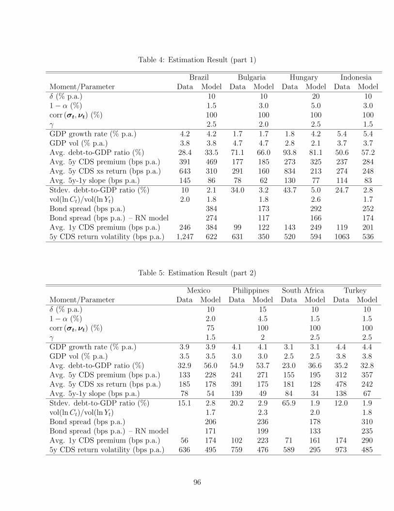
Table 4: Estimation Result (part 1)

Brazil Bulgaria Hungary IndonesiaMoment/Parameter Data Model Data Model Data Model Data Modelδ (% p.a.) 10 10 20 101− α (%) 1.5 3.0 5.0 3.0corr (σt,νt) (%) 100 100 100 100γ 2.5 2.0 2.5 1.5GDP growth rate (% p.a.) 4.2 4.2 1.7 1.7 1.8 4.2 5.4 5.4GDP vol (% p.a.) 3.8 3.8 4.7 4.7 2.8 2.1 3.7 3.7Avg. debt-to-GDP ratio (%) 28.4 33.5 71.1 66.0 93.8 81.1 50.6 57.2Avg. 5y CDS premium (bps p.a.) 391 469 177 185 273 325 237 284Avg. 5y CDS xs return (bps p.a.) 643 310 291 160 834 213 274 248Avg. 5y-1y slope (bps p.a.) 145 86 78 62 130 77 114 83Stdev. debt-to-GDP ratio (%) 10 2.1 34.0 3.2 43.7 5.0 24.7 2.8vol(lnCt)/vol(lnYt) 2.0 1.8 1.8 2.6 1.7Bond spread (bps p.a.) 384 173 292 252Bond spread (bps p.a.) – RN model 274 117 166 174Avg. 1y CDS premium (bps p.a.) 246 384 99 122 143 249 119 2015y CDS return volatility (bps p.a.) 1,247 622 631 350 520 594 1063 536

Table 5: Estimation Result (part 2)

Mexico Philippines South Africa TurkeyMoment/Parameter Data Model Data Model Data Model Data Modelδ (% p.a.) 10 15 10 101− α (%) 2.0 4.5 1.5 1.5corr (σt,νt) (%) 75 100 100 100γ 1.5 2 2.5 2.5GDP growth rate (% p.a.) 3.9 3.9 4.1 4.1 3.1 3.1 4.4 4.4GDP vol (% p.a.) 3.5 3.5 3.0 3.0 2.5 2.5 3.8 3.8Avg. debt-to-GDP ratio (%) 32.9 56.0 54.9 53.7 23.0 36.6 35.2 32.8Avg. 5y CDS premium (bps p.a.) 133 228 241 271 155 195 312 357Avg. 5y CDS xs return (bps p.a.) 185 178 391 175 181 128 478 242Avg. 5y-1y slope (bps p.a.) 78 54 139 49 84 34 138 67Stdev. debt-to-GDP ratio (%) 15.1 2.8 20.2 2.9 65.9 1.9 12.0 1.9vol(lnCt)/vol(lnYt) 1.7 2.3 2.0 1.8Bond spread (bps p.a.) 206 236 178 310Bond spread (bps p.a.) – RN model 171 199 133 235Avg. 1y CDS premium (bps p.a.) 56 174 102 223 71 161 174 2905y CDS return volatility (bps p.a.) 636 495 759 476 589 295 973 485

96

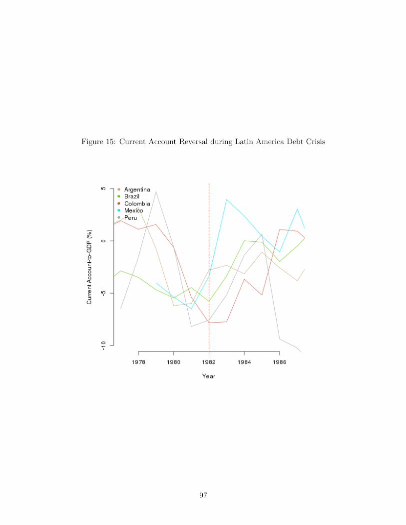
Figure 15: Current Account Reversal during Latin America Debt Crisis

97

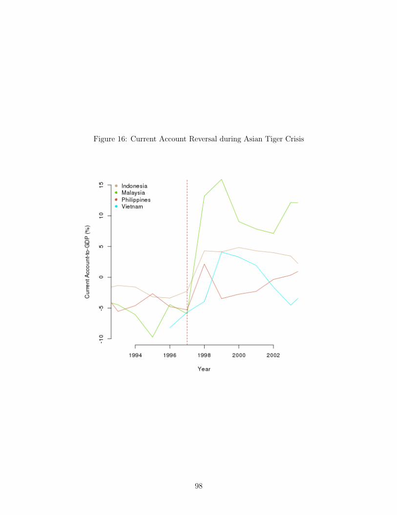
Figure 16: Current Account Reversal during Asian Tiger Crisis

98

A.3 Numerical Algorithm – Markov Chain Approximation

I will use a Markov Chain approximation method, as explained in Kushner and Dupuis

(2001). I select this method over the more traditional finite difference schemes: indeed, to

guarantee convergence of both methods to the solution of the differential equations of interest,

the latter requires using numerical schemes that are consistent, monotone and stable, and

the last two requirements are not always simple to verify 25, while the former requires the

construction of approximating Markov chains whose transition probabilities need to satisfy

consistency properties that are extremelly simple to verify in practice. I also favor the Markov

Chain approximation method over collocation methods: the latter methods require inverting

non-sparse matrices, while the former involves the inversion of sparse matrices, making my

algorithm significantly faster.

I compute the functions (vs, Ds)s≤Ns numerically over the compact set [0,maxs xs],

by determining their values on an equally-spaced grid Gh, where h > 0 is my scalar app-

proximation parameter. I will note xk = kh0≤k≤Nh the grid points of Gh. I start with

a guess equilibrium cutoff Ns × 1 vector x(1), and a guess issuance policy vector ι(1,1) =

ι(1,1)s (xk)0≤k≤Nh,0≤s≤Ns . My algorithm has an outer-loop, which updates the equilibrium

default cutoff vector x(i), and an inner loop, which, for a given vector of cutoffs x(i), up-

dates the functions v(i,j)s , D

(i,j)s , ι

(i,j)s . In the inner loop, I calculate the functions vs(·; x(i)),

Ds(·; x(i)) and ιs(·; x(i)) as follows.

I first describe how to compute D(i,j)s s≤Ns , given an issuance schedule ι(i,j) and a default

policy x(i). To simplify notation, I omit the superscript (i, j) when possible. Given a set of

cutoffs xss≤Ns and issuance policies ιss≤Ns , the dynamic evolution of the state variables

xt and st under Q can be written as follows, for xt ∈ [0, xst ]:

dxt =(ιst(xt)−

(m+ µst − |σst|2 − νst · σst

)xt)dt− xtσst · dBt

= µQ(xt, st)dt− xtσst · dBt

dst =∑s′ 6=st−

(s′ − st−)dNst−,s′

t

In the inner loop, I create a Markov Chain XhQ,n :=

(xhQ,n, s

hQ,n)

that approximates the process

(xt, st)t≥0 under Q. I introduce QhQ(x, s) and ∆thQ(x, s) as follows:

QhQ(x, s) := x2|σs|2 + h|µQ(x, s)|

∆thQ(x, s) :=h2

QhQ(x, s)

25I note however that upwinding has been used as a classic tool to implement monotone schemes.

99

Since µQ(0, s) > 0 for all discrete SDF state s (in equilibrium the sovereign will be borrowing

when it is not indebted, i.e. ιs(0) > 0), infx,sQhQ(x, s) > 0, which means that ∆thQ(x, s) is

well defined. For all x and all s ≤ Ns, I have:

limh→0

∆thQ(x, s) = 0

I then define the following transition probabilities:

Pr(Xh

Q,n+1 = (x+ h, s) |XhQ,n = (x, s)

)=eΛss∆thQ(x,s)

QhQ(x, s)

(x2|σs|2

2+ hmax (0, µQ(x, s))

)Pr(Xh

Q,n+1 = (x− h, s) |XhQ,n = (x, s)

)=eΛss∆thQ(x,s)

QhQ(x, s)

(x2|σs|2

2+ hmax (0,−µQ(x, s))

)Pr(Xh

Q,n+1 = (x, s′) |XhQ,n = (x, s)

)=

(Λss′

−Λss

)(1− eΛss∆thQ(x,s)

)Notice that these transition probabilities are all greater than zero, less than 1, and they add

up to 1. Noting ∆xhQ,n := xhQ,n+1−xhQ,n and ∆shQ,n := shQ,n+1− shQ,n, the Markov chain created

satisfies the local consistency condition:

Ex,s[∆xhQ,n

]= µQ(x, s)∆thQ(x, s) (69)

varx,s[∆xhQ,n

]= x2|σs|2∆thQ(x, s) + o

(∆thQ(x, s)

)(70)

Ex,s[∆shQ,n

]=∑s′

Λs,s′(s′ − s)∆thQ(x, s) (71)

varx,s[∆shQ,n

]=∑s′

Λs,s′(s′ − s)2∆thQ(x, s) + o

(∆thQ(x)

)(72)

covx,s[∆xhQ,n,∆s

hQ,n]

= 0 (73)

For xs > xk ≥ 0, the sovereign government is performing and I compute D(i,j)s (xk) as follows:

D(i,j)s (xk) = (κ+m)∆thQ(xk, s) + e−(rs+m)∆thQ(xk,s)

∑x′Q,s

′Q

Pr(X ′Q|xk, s

)D

(i,j)

s′Q(x′Q)

For xk ≥ xs, the sovereign government is in default and I compute D(i,j)s (xk) as follows:

D(i,j)s (xk) = λθα

(Ξ−1D(i,j)(θxk)

)s

This is a linear system ofNs×(Nh+1) equations inNs×(Nh+1) unknown D(i,j)s (xk)0≤k≤Nh,s≤Ns

which can be solved easily via a simple matrix inversion. Note that the matrix to be inverted

100

is sparse, which greatly reduces computing time.

I then describe how to compute v(i,j)s in each discrete Markov state s, given an issuance

schedule ι(i,j), a debt price schedule D(i,j) and a default policy x(i). Once again I omit the

superscript (i, j) when possible. Given a vector of cutoffs x, an issuance policy ι and a debt

price schedule D, the dynamic evolution of the state variables xt and st under the probability

measure induced via Pr(A) = E[e(1−γ)

∫ t0 σsu ·dBu− 1

2(1−γ)2

∫ t0 |σsu |2du1A

]can be expressed as

follows, for xt ∈ [0, xst ]:

dxt =(ιst(xt)−

(m+ µst − γ|σst |2

)xt)dt− xtσst · dBt

= µP(xt, st)dt− xtσst · dBt

dst =∑s′ 6=st−

(s′ − st−)dNst−,s′

t

By introducingQhP(x, s) and ∆thP(x, s), computed in a similar fashion toQh

Q(x, s) and ∆thQ(x, s),

I can construct a new Markov Chain XhP,nn≥0 that approximates the process (xt, st)t≥0

under the probability measure Pr. The transition probabilities of this Markov chain will

satisfy consistency conditions similar to those of equations (69), (70), (71), (72) and (73).

For xs > xk ≥ 0, the sovereign government is performing and I compute v(i,j)s (xk) as follows:

v(i,j)s (xk) =

δ

1− ρ(1 + ιs(xk)Ds(xk)− (κ+m)xk)

[(1− γ)v(i,j)

s (xk)] ρ−γ

1−γ ∆thP(xk, s)

+ e−1−γ1−ρAs∆t

hP

(xk,s)∑x′P,s′

P

Pr(X ′P|xk, s

)v

(i,j)

s′P

(x′P)

For xk ≥ xs, the sovereign government is in default and I compute v(i,j)s (xk) = α1−γ (vds)(i,j)

(xk)

as follows:

(vds)(i,j)

(xk) =

[Υ−1

(δ

1− ρ

[(1− γ)

(vd)(i,j)

(xk)] ρ−γ

1−γ+ λv(i,j)(θxk)

)]s

Note that the resulting system of Ns × (Nh + 1) equations in Ns × (Nh + 1) unknown

v(i,j)s (xk)0≤k≤Nh,s≤Ns is not linear. In order to solve such system, I use a simple proce-

dure: starting with a guess v(i,j,m)(xk)0≤k≤Nh , I iterate, for xk < xs, on the following:

v(i,j,m+1)s (xk) =

δ

1− ρ(1 + ιs(xk)Ds(xk)− (κ+m)xk)

[(1− γ)v(i,j,m)

s (xk)] ρ−γ

1−γ ∆thP(xk, s)

+ e−1−γ1−ρAs∆t

hP

(xk,s)∑x′P,s′

P

Pr(X ′P|xk, s

)v

(i,j,m+1)

s′P

(x′P)

101

For xk ≥ xs, the iteration becomes:

(vds)(i,j,m+1)

(xk) =

[Υ−1

(δ

1− ρ

[(1− γ)

(vd)(i,j,m+1)

(xk)] ρ−γ

1−γ+ λv(i,j,m)(θxk)

)]s

The iterative procedure is stopped once ||v(i,j,m+1) − v(i,j,m)||∞ is sufficiently small. Once

v(i,j) and D(i,j) are computed, I can update the issuance policy as follows, in each state s:

ι(i,j+1)s (xk) = $ι(i,j)s (xk) +

1−$D

(i,j)s (xk)

δD(i,j)

s (xk)[(1− γ)v

(i,j)s (xk)

] ρ−γ1−γ

−(v

(i,j)s

)′(xk)

1/ρ

+ (κ+m)xk − 1

In the above $ ∈ (0, 1) is a dampening parameter that “smoothes” the transition from ι

(i,j)s

to ι(i,j+1)s and prevents infinite loops between debt price and issuance policy26. The derivative(

v(i,j)s

)′(xk) is computed by using a centered finite difference approximation. I iterate on the

inner loop until ||ι(i,j+1) − ι(i,j)||∞ is sufficiently small.

At the conclusion of the inner loop, I have obtained v(i),D(i), ι(i), all assuming a default

policy x(i). I then set x(i+1) by checking the smooth pasting condition at x(i)s for all discrete

states s:

(v(i))′(x(i)s ) ≷ α1−γλθ

[(Υ + δ

γ − ρ1− ρ

diagj

([(1− γ)vdj (xs)

]− 1−ρ1−γ))−1

v′(θxs)

]s

Depending on whether the left handside is greater or less than the right handside, I update

x(i+1)s using a binomial search method.

Once the optimal default boundary x and the optimal issuance policy ι are known, I

can compute the expected default time and the ergodic density of x. The computation of

the expected default time T (x) follows the same logic as the computation of the debt price,

except that the Markov transition probabilities are adjusted to reflect the stochastic evolution

of xt and st under the physical measure P. Finally, the ergodic density of (xt, st) under

P is constructed as follows. First, I find the unitary eigen-vector ph(xk, s)0≤k≤Nh,1≤s≤Ns

(associated with the eigen-value 1) of the transpose of a Markov matrix whose elements

correspond to transition probabilities in and out of performing states (xk, s) (for xk ≤ xs),

as well as in and out of default states (xk, s) (for xk ≥ mins xs). Once again those transition

26For most parameter configurations of interest, the issuance policy is increasing in the debt price schedule,and the debt price is a decreasing function of the issuance schedule. Thus, without dampening, the algorithmends up frequently in an infinite loop: a high debt price at the end of iteration j leads to a high issuancepolicy in iteration j + 1; such high issuance policy feeds back into a low debt price at iteration j + 1, whichleads to a low issuance policy in iteration j + 2, thus creating the infinite loop.

102

probabilities are constructed in an identical way to those described previously. For each state

(xk, s), the ergodic density at such point is approximated by πh(xk, s), computed as follows:

πh(xk, s) :=ph(xk, s)∆t

hP(xk, s)∑

xj ,s′ph(xj, s′)∆thP(xj, s′)

In order to compute CDS prices, I use a slightly modified procedure. As described previ-

ously, I need to compute the risk-neutral expected loss Ls(x, T ) and the risk-neutral expected

present value of CDS premia Ps(x, T ). Introduce the constant ε > 0. QhQ(x, s) and ∆thQ(x, s)

are now defined as follows:

QhQ(x, s) := x2|σs|2 + h|µQ(x, s)|+ h/ε

∆thQ(x, s) :=h2

QhQ(x, s)

I still have infx,sQhQ(x, s) > 0, which means that ∆thQ(x, s) is well defined. For all x, s, I have:

limh→0

∆thQ(x, s) = 0

The state space now includes time-to-maturity T , and the approximating Markov chain is

now the three-dimentional process XhQ,n :=

(xhQ,n, s

hQ,n, T

hQ,n). Given a starting state Xh

Q,n =

(x, s, T ), I define the following transition probabilities:

Pr(Xh

Q,n+1 = (x+ h, s, T )|XhQ,n)

=eΛss∆thQ(x,s)

QhQ(x, s)

(x2|σs|2

2+ hmax (0, µQ(x, s))

)Pr(Xh

Q,n+1 = (x− h, s, T )|XhQ,n)

=eΛss∆thQ(x,s)

QhQ(x, s)

(x2|σs|2

2+ hmax (0,−µQ(x, s))

)Pr(Xh

Q,n+1 = (x, s, T − εh)|XhQ,n)

=eΛss∆thQ(x,s)h/ε

QhQ(x, s)

Pr(Xh

Q,n+1 = (x, s′, T ) |XhQ,n)

=

(Λss′

−Λss

)(1− eΛss∆thQ(x,s)

)Notice that these transition probabilities are all greater than zero, less than 1, and they add

up to 1. The Markov chain created satisfies local consistency conditions similar to those in

equations (69), (70), (71), (72) and (73), in addition to:

Es,x[∆T hQ,n

]= −∆thQ(x, s)

vars,x[∆T hQ,n

]= o

(∆thQ(x, s)

)103

The state space gridGh is three-dimensional, and is of the form (xi, s, Tj)1≤i≤Nx,h,1≤s≤Ns,1≤j≤NT,h ,

where the grid points xi and the grid points Tj are equally spaced with distance h and

εh respectively. For xs > xi ≥ 0 and for T ≥ Ti > 0, I compute Ls(xi, Tj) and Ps(xi, Tj) on

the grid Gh as follows:

Ls(xi, Tj) = e−rs∆thQ(xi,s)

∑(x′Q,s′Q,T ′Q)

Pr(X ′Q|(xi, s, Tj)

)Ls′Q

(x′Q, T

′Q)

Ps(xi, Tj) = ∆thQ(xi, s) + e−rs∆thQ(xi,s)

∑(x′Q,s′Q,T ′Q)

Pr(X ′Q|(xi, s, Tj)

)Ps′Q

(x′Q, T

′Q)

I note xNx,h,s the grid point at which the sovereign government defaults optimally in state s, in

other words Nx,h,s = xs/h. The boundary conditions at T = 0 are Ls(xi, 0) = 0 for i < Nx,h,s,

Ls(xi, 0) = (1−D(xi)) for i ≥ Nx,h,s, and Ps(xi, 0) = 0 for all xi. The boundary conditions at

T > 0 are Ls(xi, T ) = (1−D(xi)) and Ps(xi, T ) = 0 for i ≥ Nx,h,s and for any T . This system

of linear equations is solved recursively: starting from Ls(xi, 0), Ps(xi, 0)1≤i≤Nx,h,s≤Ns , I can

compute Ls(xi, εh), P (xi, εh)1≤i≤Nx,h,s≤Ns via the system of linear equations above, and

progress backwards.

104

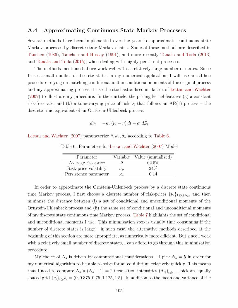
A.4 Approximating Continuous State Markov Processes

Several methods have been implemented over the years to approximate continuous state

Markov processes by discrete state Markov chains. Some of these methods are described in

Tauchen (1986), Tauchen and Hussey (1991), and more recently Tanaka and Toda (2013)

and Tanaka and Toda (2015), when dealing with highly persistent processes.

The methods mentioned above work well with a relatively large number of states. Since

I use a small number of discrete states in my numerical application, I will use an ad-hoc

procedure relying on matching conditional and unconditional moments of the original process

and my approximating process. I use the stochastic discount factor of Lettau and Wachter

(2007) to illustrate my procedure. In their article, the pricing kernel features (a) a constant

risk-free rate, and (b) a time-varying price of risk νt that follows an AR(1) process – the

discrete time equivalent of an Ornstein-Uhlenbeck process:

dνt = −κν (νt − ν) dt+ σνdZt

Lettau and Wachter (2007) parameterize ν, κν , σν according to Table 6.

Table 6: Parameters for Lettau and Wachter (2007) Model

Parameter Variable Value (annualized)Average risk-price ν 62.5%

Risk-price volatility σν 24%Persistence parameter κν 0.14

In order to approximate the Ornstein-Uhlenbeck process by a discrete state continuous

time Markov process, I first choose a discrete number of risk-prices νi1≤i≤Ns , and then

minimize the distance between (i) a set of conditional and unconditional moments of the

Ornstein-Uhlenbeck process and (ii) the same set of conditional and unconditional moments

of my discrete state continuous time Markov process. Table 7 highlights the set of conditional

and unconditional moments I use. This minimization step is usually time consuming if the

number of discrete states is large – in such case, the alternative methods described at the

beginning of this section are more appropriate, as numerically more efficient. But since I work

with a relatively small number of discrete states, I can afford to go through this minimization

procedure.

My choice of Ns is driven by computational considerations – I pick Ns = 5 in order for

my numerical algorithm to be able to solve for an equilibrium relatively quickly. This means

that I need to compute Ns × (Ns − 1) = 20 transition intensities (Λij)i 6=j. I pick an equally

spaced grid νii≤Ns = (0, 0.375, 0.75, 1.125, 1.5). In addition to the mean and variance of the

105

Table 7: Target Moments

Moment Lettau and Wachter (2007) Model Discrete State Model

E [νt] ν∑Ns

i=1 πiνi

var [ν2t ] σ2

ν

2κν

∑Nsi=1 πiν

2i −

(∑Nsi=1 πiνi

)2

E [νt+s|Ft] νte−κνs + ν (1− e−κνs)

∑Nsj=1

(eΛs)st,j

νj

var [νt+s|Ft] σ2ν

2κν(1− e−2κνs)

∑Nsj=1

(eΛs)st,j

ν2j −

(∑Nsj=1

(eΛs)st,j

νj

)2

ergodic distribution of νt, I also match the conditional mean and variance at 2 horizons: 0.25

years, and 2 years. This gives me 22 different moments (20 conditional, and 2 unconditional),

for 20 free parameters. My approximation procedure leads to the following generator matrix:

Λ =

−0.1838 0.1637 0.0075 0.0012 0.0113

0.0703 −0.1576 0.034 0.0401 0.0132

0.0417 0.0904 −0.2505 0.1154 0.003

0.0239 0.002 0.1406 −0.1826 0.016

0.0001 0.0001 0.0772 0.1412 −0.2186

The resulting ergodic distribution π is displayed in Figure 17. The ergodic distribution of my

discrete state process has a mean of 62.5% and a standard deviation of 45%, which correspond

exactly to the moments of the ergodic distribution of the original Ornstein Uhlenbeck process.

The maximum relative error in conditional means is equal to 1.7%, while the maximum

relative error in conditional variances is equal to 7.9%.

Finally, I highlight one particular aspect of the SDF used in this paper: its persistence.

Consistent with many models of the stochastic discount factor, whether long-run risk models,

habit formation models, or more reduced form specifications such as Lettau and Wachter

(2007), the persistence of the risk-price process is high – in the particular parametrization

of Lettau and Wachter (2007), the half-life mean-reversion speed is ln 2/κν ≈ 5 years. This

feature of asset pricing models has its importance in the context of my sovereign default

framework: since the transition intensities in and out of a given state are relatively small,

the adjustments to the sovereign financing policy will be larger than if those intensities were

higher. This will lead to the relatively large current account adjustments discussed in the

core of my paper. Note that the autocorrelation function of my discrete state continuous

106

Figure 17: Stationary Distribution

time Markov process approximation takes the following form:

R(s) =

∑Nsi=1 πiνi

∑Nsj=1

[(esΛ)ij− πj

]νj∑Ns

i=1 πiν2i −

(∑Nsi=1 πiνi

)2

One can show that asymptotically, R(s) ≈ e−κs, where −κ is the largest non-zero (and of

course negative) eigen-value of the matrix Λ. My numerical procedure leads to κ = 0.139,

which is very close to the persistence parameter κν = 0.14 in the original article of Lettau and

Wachter (2007). I display R(s) in Figure 18, and on the same graph I plot the autocorrelation

function of the original Ornstein-Uhlenbeck process, simply equal to e−κνs. As showed in the

plot, the two autocorrelation functions are indistinguishable.

107

Figure 18: Autocorrelation Function

108