Macroeconometric modelling for policy

Gunnar Bårdsen and Ragnar Nymoen∗

Working Paper, 30 April, 2008

Abstract

The first part of this chapter sets out a coherent approach to dynamic macroecono-metric model building; the second part demonstrates the approach through buildingand evaluating a small econometric model; the final part demonstrates various usagesof the model for policy.

Contents

1 Introduction 3

2 A modelling framework 62.1 Linearization . . . . . . . . . . . . . . . . . . . . . . . . . . . . . . . . . . . 72.2 Discretization . . . . . . . . . . . . . . . . . . . . . . . . . . . . . . . . . . . 72.3 Equilibrium correction representations and cointegration . . . . . . . . . . . 82.4 System representations . . . . . . . . . . . . . . . . . . . . . . . . . . . . . . 92.5 From a discretized and linearized cointegrated VAR representation to a

dynamic SEM in three steps . . . . . . . . . . . . . . . . . . . . . . . . . . . 102.5.1 First step: the statistical system . . . . . . . . . . . . . . . . . . . . 112.5.2 Second step: the overidentified steady state . . . . . . . . . . . . . . 112.5.3 Third step: the dynamic SEM . . . . . . . . . . . . . . . . . . . . . 12

2.6 Example: The supply side of a medium term macroeconomic model . . . . 122.6.1 Economic theory . . . . . . . . . . . . . . . . . . . . . . . . . . . . . 122.6.2 Cointegration and long-run identification . . . . . . . . . . . . . . . 152.6.3 VAR and identified equilibrium correction system . . . . . . . . . . . 162.6.4 Economic interpretation of the steady state . . . . . . . . . . . . . . 182.6.5 Implementation in NAM . . . . . . . . . . . . . . . . . . . . . . . . . 21

3 Building a model for monetary policy analysis 223.1 The model and its transmission mechanisms . . . . . . . . . . . . . . . . . . 223.2 Steady state . . . . . . . . . . . . . . . . . . . . . . . . . . . . . . . . . . . . 263.3 Stability of the steady state . . . . . . . . . . . . . . . . . . . . . . . . . . . 28

4 Macroeconometric models as tools for policy analysis 294.1 Tractability: Stylized representations . . . . . . . . . . . . . . . . . . . . . . 294.2 Shock analysis: Dynamic simulations . . . . . . . . . . . . . . . . . . . . . . 32

4.2.1 How strong is the policy instrument? . . . . . . . . . . . . . . . . . . 324.2.2 Fitting the facts . . . . . . . . . . . . . . . . . . . . . . . . . . . . . 324.2.3 Shock analysis with dynamic multipliers . . . . . . . . . . . . . . . . 33

∗Bårdsen: Norwegian University of Science and Technology, Trondheim. Nymoen: University of Oslo.We thank Q. Farooq Akram and Kerry Patterson for helpful comments and discussions. Prepared forPalgrave Handbook of Econometrics Vol. 2 . Please do not quote or circulate.

1

4.3 Aspects of optimal policy: The impact of model specification on optimalmonetary policy . . . . . . . . . . . . . . . . . . . . . . . . . . . . . . . . . . 34

4.4 Theory evaluation: The New Keynesian Phillips curve . . . . . . . . . . . . 374.4.1 The New Keynesian Phillips curve . . . . . . . . . . . . . . . . . . . 374.4.2 The equilibrium correction implications of the NPC . . . . . . . . . 394.4.3 Testing the equilibrium correction implications of the NPC . . . . . 40

4.5 Forecasting for monetary policy . . . . . . . . . . . . . . . . . . . . . . . . . 414.5.1 Assumptions about the forecasting situation . . . . . . . . . . . . . . 424.5.2 Real-time forecast performance . . . . . . . . . . . . . . . . . . . . . 434.5.3 Ex post forecast evaluation and robustification. . . . . . . . . . . . . 46

5 Conclusion 52

A Data definitions and equation statistics 53A.1 Variables . . . . . . . . . . . . . . . . . . . . . . . . . . . . . . . . . . . . . 53A.2 Notation for estimation and mispecification tests . . . . . . . . . . . . . . . 54

2

“I think it should be generally agreed that a model that does not gen-erate many properties of actual data cannot be claimed to have any ‘policyimplications’...”Clive.W. J. Granger (1992), p. 4.

1 Introduction

Depending upon its properties, a macroeconometric model can highlight various aspectsof economic policy: communication of policy actions, structuring of economic debate,policy simulations, testing of competing theories, forecasting, stress testing, and so on.From an academic perspective, the desired properties of a model are also legion, butthe end result will depend upon the preferences for coherence along dimensions like:theory foundations (microfoundations/aggregation/general/partial), econometric methods(Bayesian/classical), and model properties (size/robustness/non-linearities/transparency/dynamics)

Satisfying the different needs and desires of policy-making could therefore entail a col-lection of models. Such a model collection could include more or less calibrated theorymodels, Structural and Bayesian Vector Autoregressions (VARs), Simultaneous EquationModels(SEMs), and Dynamic Stochastic General Equilibrium (DSGEs) models–see Pa-gan (2003) for an overview.. A choice of model(s) for the event at hand could then bemade on the basis of strengths and weaknesses of the various candidates. The inherentweaknesses of the main candidates are well known. If one were to follow Ambrose Bierce,and write a “Devil’s Dictionary” of macroeconometrics, some of the entries could read:Structural VARs: How to estimate models inefficiently; SEMs: Estimates of something;Bayesian estimation: See calibration; DSGEs: Sophisticated naivety. Therefore, a choiceof model(s) for the event at hand should be made on the basis of strengths and weaknessesof the various model classes.

The profession’s collective understanding of the causes and possible remedies of modellimitations, both in forecasting or in policy analysis, has improved markedly over the lastdecades. The Lucas (1976) critique and the Clements and Hendry (1999) analysis of thesources of forecast failures with macroeconometric models are milestones in that process.Interestingly, the methodological ramifications of those two critiques are different: TheLucas-critique have led to the current dominance of representative agents based macro-economic models. Hendry (2001a), on the other hand, concludes that macroeconometricsystems of equations, despite their vulnerability to regime shifts, but because of theirpotential adaptability to breaks, remain the best long-run hope for progress in macro-economic forecasting. Since monetary policy can be a function of the forecasts, as withinflation forecast targeting, cf. Svensson (1997), the choice of forecasting model(s) isimportant.

The class of macroeconometric models we present in this chapter requires coherent useof economic theory, data, and mathematical and statistical techniques. This approach ofcourse has a long history in econometrics, going back to Tinbergen’s first macroecono-metric models, and have enjoyed renewed interest in the last decades. Recent advancesin econometrics and in computing means that we now are much better tools than say 20years ago, for developing and maintaining macroeconometric models in this tradition–seeGarratt et al. (2006) for one recent approach.

Regardless of underlying theory, a common aim of macroeconometric model building isidentification of invariant relationships, if they exist at all, see Haavelmo (1944, ChapterII). A well-specified macroeconometric model is a good starting point of such a quest,since it provides an ideal test bed for further overidentifying restrictions of microeconomicbehaviour. Such a strategy is in particular relevant with the challenges from behaviouraleconomics, with implications like: time inconsistency (hyperbolic discounting), changing

3

expectations (learning), asset bubbles (herd behaviour), and so on.Macroeconomic models of the representative agent, intertemporal optimizing, type are

said to have structural interpretations, with ‘deep structural parameters’ that are immuneto the Lucas critique. However, when the model’s purpose is to describe the observedmacroceconomic behaviour, its structural properties are conceptually different. Heuristi-cally, we take a model to have structural properties if it is invariant and interpretable–seeHendry (1995b). Structural properties are nevertheless relative to the history, the natureand the significance of regime shifts. There is always the possibility that the next shocksto the system may incur real damage to a model with high structural content hitherto.The approach implies that a model’s structural properties must be evaluated along severaldimensions, and the following seem particularly relevant:

1. Theoretical interpretation.

2. Ability to explain the data.

3. Ability to explain earlier findings, i.e., encompassing the properties of existing modes.

4. Robustness to new evidence in the form of updated/extended data series and neweconomic analysis suggesting e.g., new explanatory variables.

Economic analysis (#1) is an indispensable guidance in the formulation of economet-ric models. Clear interpretation also helps communication of ideas and results amongresearchers, in addition to structuring debate. However, since economic theories are nec-essarily simplifying abstractions, translations of theoretical to econometric models mustlead to problems like biased coefficient estimates, wrong signs of coefficients, and/or resid-ual properties that hampers valid inference. The main distinction seems to be betweenseeing theory as representing the correct specification, (leaving parameter estimation tothe econometrician), and viewing theory as a guideline in the specification of a modelwhich also accommodates institutional features, attempts to accommodate heterogeneityamong agents, addresses the temporal aspects for the data set and so on–see Granger(1999).

Arguments against “largely empirical models” include sample dependency, lack of in-variance, unnecessary complexity (in order to fit the data) and chance finding of “signifi-cant” variables. Yet, ability to characterize the data (#2) remains an essential quality ofuseful econometric models, and given the absence of theoretical truisms, the implicationsof economic theory have to be confronted with the data in a systematic way.

We use cointegration methods on linearized and discretized dynamic systems to esti-mate theory-interpretable and idenitifed steady state relationships, imposed in the formof equilibrium-correction models. We also make use of an automated model-selectionapproach to sift out the best theory-interpretable and identified dynamic specifications.Hoover and Perez (1999), Hendry and Krolzig (1999) and Doornik (2008) have shown thatautomated model selection methods has a good chance of finding a close approximation tothe data generating process, and that the danger of over-fitting is in fact (surprisingly) low.Conversely, acting as if the specification is given by theory alone, with only coefficientestimates left to “fill in”, is bound to result in the econometric problems noted above, andto a lower degree of relevance of the model for the economy it claims to represent.

In order to develop scientific basis for policy modelling in macroeconometrics, a newmodel’s capability of encompassing earlier findings should be regarded as an importantaspect of structure (#3). There are many reasons for the coexistence of contested mod-els for the same phenomena, some of which may be viewed as inherent (limited numberof data observations, measurement problems, controversy about operational definitions,new theories). Nevertheless, the continued use a corroborative evaluation (i.e., only ad-dressing goodness of fit or predicting the stylized fact correctly) may inadvertently hinder

4

cumulation of evidence taking place. One suspects that there would be huge gains from abreakthrough for new standards of methodology and practice in the profession.

Ideally, empirical modelling is a cumulative process where models continuously be-come overtaken by new and more useful ones. By useful, we understand in particularmodels that are relatively invariant to changes elsewhere in the economy, i.e., they containautonomous parameters, see Haavelmo (1944), Johansen (1977), Aldrich (1989), Hendry(1995b). Models with a high degree of autonomy represent structural properties: Theyremain invariant to changes in economic policies and other shocks to the economic system,as implied by #4 above.1 However, structure is partial in two respects: First, autonomyis a relative concept, since an econometric model cannot be invariant to every imaginableshock. Second, all parameters of an econometric model are unlikely to be equally invari-ant, and only the parameters with the highest degree of autonomy represent structure.Since elements of structure typically will be grafted into equations that also contain pa-rameters with a lower degree of autonomy, forecast breakdown may frequently be causedby shifts in these non-structural parameters.2

A strategy for model evaluation that puts a lot of emphasis on forecast behaviour,without a careful evaluation of the causes of forecast failure ex post, runs a risk of discardingmodels that actually contain important elements of structure. Hence, for example Doornikand Hendry (1997) and Clements and Hendry (1999, Ch. 3) show that the main sourceof forecast failure is location shifts (shifts in means of levels, changes, etc.), and not shiftsin such coefficients that are of primary concern in policy analysis, i.e., the derivativecoefficients of behavioural equations. Therefore, a rough spell in terms of forecastingperformance does not by itself disqualify the model’s relevance for policy analysis. If thecause of the forecast failure is location shifts, they can be attenuated ex post by interceptcorrection or additional differencing ‘within’ the model, Hendry (2004). With these add-ons, and once the break-period is in the information set, the model forecast will adaptto the new regime and improve again. Failure to adapt to the new regime, may thenbe a sign of a deeper source of forecast failure, in the form of non-constant derivativecoefficients which also undermines the models relevance for policy analysis.3 In general,without adaptive measures, models with high structural content will lose regularly tosimple forecasting rules, see e.g., Clements and Hendry (1999), Eitrheim et al. (1999).Hence different models may be optimal for forecasting and for policy analysis, which fitswell with the often heard recommendation of a suite of monetary policy models.

Structural breaks are always a main concern in econometric modelling, but like anyhypothesis of theory, the only way to judge the significance of a hypothesized break isby confrontation with the evidence in the data. Moreover, given that an encompassingapproach is followed, a forecast failure is not only destructive but represent a potential forimprovement, if successful respecification follows in its wake, cf. Eitrheim et al. (2002). Inthe same vein, one important intellectual rationale for DSGE models is the Lucas critique.If the Lucas critique holds, any "reduced-form" equation in a model is liable to be unstablealso over the historical sample, due to regime shifts and policy changes that have takenplace in the economy. Hence according to the Lucas critique, parameter instability maybe endemic in any model that fails to obey the Rational Expectations Hypothesis (REH),with the possible consequence that without integration of REH, the model is unsuited forpolicy analysis. However, as stated by Ericsson and Irons (1995), the Lucas critique is onlya possibility theorem, not a truism, and that the implications of the Lucas critique can be

1see e.g., Hendry (1995a, Ch. 2,3 and 15.3) for a concise definition of structure as the invariant set ofattributes of the economic mechanism.

2This line of thought may lead to the following practical argument against large-scale empirical models:Since modelling resources are limited, and some sectors and activities are more difficult to model thanothers, certain euations of any given model are bound to have less structural content than others, i.e., themodel as a whole is no better than its weakest (least structural) equation.

3See Nymoen (2005) for an analysis of a recent failure in inflation forecasting.

5

tested, see also for example Hendry (1988), Engle and Hendry (1993) and Ericsson andHendry (1999). In Bårdsen et al. (2003) we have shown, by extensive testing of a previousversion, that the Lucas critique has little force for our system of equations. This findingis consistent with the international evidence presented in Ericsson and Irons (1995) andStanley (2000). On the basis of these results, our model is more consistent with agentsadopting robust forecasting rules, in line with the analysis and suggestions of Hendryand Mizon (2000). In that case the Lucas critique does not apply, although the degreeof autonomy remains an issue that needs to be evaluated as fully as possible, given theinformation available to us.

This chapter documents the approach we use to dynamic macroeconometric modelbuilding and policy analysis. To make the analysis applied, the approach is illustratedthrough a model of the Norwegian economy. Our approach is of course applicable toother economies, but we know more about market characteristics, policy changes andinstitutional development in Norway, than in any other country or economic area. Andsince such factual knowledge is an indispensable and complementary aid and to formaleconometrics in the building of an empirical model, we prefer to work with the economywe have most knowledge about.

The rest of the chapter consists of three main parts. The first part sets out a coherentapproach to dynamic macroeconometric model building; the second part demonstratesthe approach through building and evaluating a small econometric model; the final partdemonstrates various tools for policy analysis using the model. The first part involvesthree steps in going from general to specific. The first step is theoretical and establishesa framework for linearizing and discretizing an approximation to a general theory modelwith constant steady state values. The second step is to estimate, and solve, the steady-state model in the form of overidentifying cointegrating relationships and common trends.The third step is to identify and estimate the dynamic structure of the model.

The second part of the chapter illustrates the approach set out in the first part by theconstruction and evaluation of a small open-economy model.

The final part demonstrates five tools for policy using the model: tractability; simula-tions of policy responses; optimal policy considerations; theory evaluation, and forecasting.The first use is illustrated by introducing a method to construct stylized versions of com-plex models. The second use is illustrated by evaluating responses to monetary policyshocks. The third use shows how important model specification is for the derivation ofoptimal monetary policy. The fourth aspect is illustrated by testing the New KeynesianPhillips Curve. The final use evaluates possible sources affecting forecast performance.

2 A modelling framework

As the values of all major economic variables are announced regularly, it is easy to believethat a local approximation to a Data Generating Process (DGP) can exist. It is aninteresting philosophical question whether the true generating mechanism can (ever) becompletely described, but the usefulness of the concept does not hinge on the answer tothat question. The main point is that once the real economic world, in its enormous, ever-changing, complexity, is accepted as a premise for macroeconomic modelling, it follows thatthe main problems of macroeconometrics are model specification and model evaluation,rather than finding the best estimator under the assumption that the model is identicalto the data generating process.

The local DGP is changing with the evolution of the real world economy–throughtechnical progress, changing pattern of family composition and behaviour and politicalreform. Sometimes society evolves gradually and econometric models are then usuallyable to adapt to the underlying real-life changes, i.e. the without any noticeable loss in“usefulness” Often, however, society evolves so quickly that estimated economic relation-

6

ships break down and cease to be of any aid in understanding the current macro economyand in forecasting its development even over the first couple of years. In this case wespeak of a changing local approximation in the form of a regime shift in the generatingprocess, and a structural break in the econometric model. Since the complexity of the truemacroeconomic mechanism, and the regime shifts also contained in the mechanism, leadus to conclude that any model will at best be a local approximation to the data gener-ating process, judging the quality of, and choosing between, the approximations becomescentral.

In the rest of this section we present our approach to finding a local approximationuseful for policy.4

2.1 Linearization

Consider a very simple example of an economic model in the form of the differentialequation

dy

dt= f(y, x) , x = x(t) , (1)

in which a constant input x = x induces y(t) to approach asymptotically a constant statey as t → ∞. Clearly x and y satisfy f(y, x) = 0. For example, standard DSGE modelsusually take this form, with the models having deterministic steady state values. The usualprocedure then is to expand the differential (or difference) equation about this steady-statesolution (see, for example, Campbell (1994) or Uhlig (1999)). Employing this procedureyields

f(y, x) = f(y, x) +∂f(y, x)

∂y(y − y) +

∂f(y, x)

∂x(x− x) +R (2)

where

R =1

2!

µ∂2f(ξ, η)

∂x2(x− x)2 + 2

∂2f(ξ, η)

∂x∂y(x− x)(y − y) +

∂2f(ξ, η)

∂y2(y − y)2

¶and (ξ, η) is a point such that ξ lies between y and y while η lies between x and x. Since yand x are the steady-state values for y and x respectively, then the expression for f(y, x)takes the simplified form

f(y, x) = a (y − y) + δ (x− x) +R (3)

where a = ∂f(y, x)/∂y and δ = ∂f(y, x)/∂x are constants.If f is a linear function of y and x then R = 0 and so

f(x, y) = a

µy − y +

δ

a(x− x)

¶= a (y − bx− c) , (4)

in which b = −δ/a and c = y + (δ/a)x.

2.2 Discretization

For a macroeconometric model, a discrete representation is usually practical, and it canbe worked out as follows. Let t1, t2, · · · , tk, · · · be a sequence of times spaced h apartand let y1, y2, · · · , yk, · · · be the values of a continuous real variable y(t) at these times.The backward-difference operator 4 is defined by the rule

4yk = yk − yk−1 , k ≥ 1 . (5)

4Section 2.1-2.4 draws on Bårdsen et al. (2004a).

7

By observing that yk = (1 −4)0 yk and yk−1 = (1 −4)1 yk, the value of y at the inter-mediate point t = tk − sh (0 < s < 1) may be estimated by the interpolation formula

y(tk − sh) = yk−s = (1−4)s yk , s ∈ [0, 1] . (6)

When s is not an integer, (1 − 4)s should be interpreted as the power series in thebackward-difference operator obtained from the binomial expansion of (1 − x)s. This isan infinite series of differences. Specifically

(1−4)s = 1− s4− s(1− s)

2!42 − s(1− s)(2− s)

3!43 − · · · . (7)

With this preliminary background, the differential equation

dy

dt= f(y, x) , x = x(t) , (8)

may be integrated over the time interval [tk, tk+1] to obtain

y(tk+1)− y(tk) = 4yk+1 =

Z tk+1

tk

f(y(t), x(t)) dt (9)

in which the integral on the right hand side of this equation is to be estimated by usingthe backward-difference interpolation formula given in equation (7). The substitutiont = tk + sh is now used to change the variable of this integral from t ∈ [tk, tk+1] tos ∈ [0, 1]. The details of this change of variable areZ tk+1

tk

f(y(t), x(t)) dt =

Z 1

0f(y(tk + sh), x(tk + sh)) (hds) = h

Z 1

0fk+s ds

where fk+s = f(y(tk + sh), x(tk + sh)). The value of this latter integral is now computedusing the interpolation formula based on (7). ThusZ 1

0fk+s ds =

Z 1

0(1−4)−s fk ds

=

Z 1

0

µfk + s4fk +

s(1 + s)

2!42fk +

s(1 + s)(2 + s)

3!43fk + · · ·

¶ds

= fk +1

24fk +

5

1242fk +

3

843fk + · · · .

The final form for the backward-difference approximation to the solution of this differentialequation is therefore

4yk+1 = hfk +h

24fk +

5h

1242fk +

3h

843fk + · · · . (10)

2.3 Equilibrium correction representations and cointegration

The discretization scheme (10) applied to the linearized model (3), with k = t − 1 andh = 1, gives the equilibrium correction model, EqCM, representation

4yt = a (y − bx− c)t−1 +Rt−1 +1

2a(4yt−1 − b4xt−1) +

1

24Rt−1

+5

12a(42yt−1 − b42xt−1) +

5

1242Rt−1 + · · · .

At this point two comments are in place. The first is that an econometric specificationwill mean a truncation of the polynomial both in terms of powers and lags. Diagnostic

8

testing is therefore imperative to ensure a valid local approximation, and indeed to testthat the statistical model is valid, see Hendry (1995a, p. 15.1) and Spanos (2008). Thesecond is that the framework allows for flexibility regarding the form of the steady state.The standard approach in DSGE-modelling has been to filter the data, typically using theso-called Hodrick-Prescott filter, to remove trends, hopefully achieving stationary serieswith constant means, and then work with the filtered series. Another approach, popularat present, is to impose the theoretical balanced growth path of the model on the data,expressing all series in terms of growth corrected values. However, an alternative approachis to estimate the balanced growth paths in terms of finding the number of common trendsand identifying and estimating cointegrating relationships. The present approach allowsfor all of these interpretations.

To illustrate the approach in terms of cointegration, consider real wages to be influencedby productivity, as in many theories.5 Assume that the logs of the real wage rwt andproductivity zt are each integrated of order one, but found to be cointegrated, so

rwt ∼ I (1) , ∆rwt ∼ I (0) (11)

zt ∼ I (1) , ∆zt ∼ I (0) (12)

(rw − βz)t ∼ I (0) . (13)

Letting yt ≡ (rw − βz)t and xt ≡ ∆zt then gives

∆rwt = −ac+ a(rw − βz)t−1 +a

24 (rw − βz)t−1 + β∆zt − ab4zt−1 −

ab

2∆2zt−1 + · · · .

2.4 System representations

The approach easily generalizes to a system representation. For ease of exposition, weillustrate the two-dimensional case for which y1 → y1 and y2 → y2 as t→∞. Expandingwith respect to y1 and y2 about their steady-state values yields⎡⎣ f1 (y1, y2)

f2 (y1, y2)

⎤⎦ =⎡⎣ f1 (y1, y2)

f2 (y1, y2)

⎤⎦+⎡⎢⎣

∂f1(y1, y2)

∂y1

∂f1(y1, y2)

∂y2∂f2(y1, y2)

∂y1

∂f2(y1, y2)

∂y2

⎤⎥⎦⎡⎣ y1 − y1

y2 − y2

⎤⎦+⎡⎣ R1

R2

⎤⎦ ,where

£R1, R2

¤0 denotes the vector1

2!

⎡⎢⎢⎣∂2f1(ζ, η)

∂y21(y1 − y1)

2 + 2∂2f1(ζ, η)

∂y1∂y2(y1 − y1) (y2 − y2) +

∂2f1 (ζ, η)

∂y22(y2 − y2)

2

∂2f2 (ζ, η)

∂y21(y1 − y1)

2 + 2∂2f2 (ζ, η)

∂y1∂y2(y1 − y1) (y2 − y2) +

∂2f2 (ζ, η)

∂y22(y2 − y2)

2

⎤⎥⎥⎦so that ⎡⎢⎣ ∂y1

∂t∂y2∂t

⎤⎥⎦ =⎡⎣ α11 α12

α21 α22

⎤⎦⎡⎣ y1 − y1

y2 − y2

⎤⎦+⎡⎣ R1

R2

⎤⎦ .5Presently, we let the unemployment rate be constant and disregard it for simplicity. We return to the

role of the rate of unemployment in paragraph 2.6 below.

9

The backward-difference approximation to the solution of the system of differential equa-tions gives the system in EqCM form6, namely,

∙4y14y2

¸t

=

∙−α11c1−α22c2

¸+

∙α11 00 α22

¸ ∙y1 − δ1y2y2 − δ2y1

¸t−1

+

⎡⎣ R1

R2

⎤⎦t−1

+1

2

∙α11 α12α21 α22

¸ ∙∆y1∆y2

¸t−1

+

⎡⎣ ∆R1∆R2

⎤⎦t−1

+5

12

∙α11 α12α21 α22

¸ ∙∆2y1∆2y2

¸t−1

+

⎡⎣ ∆2R1∆2R2

⎤⎦t−1

+3

8

∙α11 α12α21 α22

¸ ∙∆3y1∆3y2

¸t−1

+

⎡⎣ ∆3R1∆3R2

⎤⎦t−1

+ · · · .

withc1 = (y1 + δ1y2) , δ1 =

α12α11

c2 = (y2 + δ2y1) , δ2 =α21α22

As before, the variables y1 and y2 can be considered as stationary functions of non-stationary components–cointegration is imposed upon the system. Consider the previousexample, assuming linearity, so Ri = 0, and ignoring higher order dynamics for ease ofexposition: ∙

4y14y2

¸t

=

∙−α11c1−α22c2

¸+

∙α11 00 α22

¸ ∙y1 − δ1y2y2 − δ2y1

¸t−1∙

4(rw − βz)∆2z

¸t

=

∙−α11c1−α22c2

¸+

∙α11 00 α22

¸ ∙(rw − βz)− δ1∆z∆z − δ2(rw − βz)

¸t−1

or multiplied out:

4rwt = −α11c1 + α11(rw − βz)t−1 + β∆zt − α12∆zt−1

∆zt = −α22µy2 +

α21α22

y1

¶+ (α22 − 1) ∆zt−1 − α21(rw − βz)t−1

So if α21 = 0 and |α22 − 1| < 1 the system simplifies to the familiar expositon of a bivariatecointegrated system with z being weakly exogenous for β:

4rwt = −α11c1 + α11(rw − βz)t−1 + β∆zt − α12∆zt−1

∆zt = −α22 z + (α22 − 1) ∆zt−1

and where the common trend is a productivity trend.

2.5 From a discretized and linearized cointegrated VAR representationto a dynamic SEM in three steps

We will keep this section brief, as comprehensive treatments can be found many places–for example in Hendry (1995a), Johansen (1995, 2006), Juselius (2007), Garratt et al.(2006), and Lütkepohl (2006)–and only make some comments on issues in each step inthe modelling process we believe merit further attention.

6See Bårdsen et al. (2004a) for details.

10

2.5.1 First step: the statistical system

Our starting point for identifying and building a macroeconometric model is to find a lin-earized and discretized approximation as a data-coherent statistical system representationin the form of a cointegrated VAR

∆yt = c+Πyt−1 +kXi=1

Γt−i∆yt−i + ut, (14)

with independent Gaussian errors ut as a basis for valid statistical inference about eco-nomic theoretical hypotheses.

The purpose of the statistical model (14) is to provide the framework for hypothesistesting, the inferential aspect of macroeconometric modelling. However, it cannot be pos-tulated directly, since the cointegrated VAR itself rests on assumptions. Hence, validationof the statistical model is an essential step: Is a model which is linear in the parame-ters flexible enough to describe the fluctuations of the data? What about the assumedconstancy of parameters, does it hold over the sample that we have at hand? And theGaussian distribution of the errors, is that a tenable assumption so that (14) can supplythe inferential aspect of modelling with sufficient statistics. The main intellectual rationalefor the model validation aspect of macroeconometrics is exactly that the assumptions ofthe statistical model requires separate attention, Johansen (2006),Spanos (2006) In prac-tice, one important step in model validation is to make the hypothesized statistical modelsubject to a battery of misspecification tests using the OLS residuals ut as data.7

As pointed out by Garratt et al. (2006), the representation ( 14) does not precludeforward-looking behaviour in the underlying model, as rational expectations models havebackward-looking solutions. The coefficients of the solution will be defined in specific waysthough, and this entails restrictions on the VAR which can utilized for testing rationalexpectations, see Johansen and Swensen (1999) and Johansen and Swensen (2004).

Even with a model which for many practical purpose is small scale it is usually too bigto be formulated in “one go” within a cointegrated VAR framework. Hence, model (14)for example is not interpretable as one rather high dimensional VAR, with the (incredible)long lags which would be needed to capture the complicated dynamic interlinkages of areal economy. Instead, as explained in Bårdsen et al. (2003), our operational procedure isto partition the (big) simultaneous distribution function of markets and variables: prices,wages, output, interest rates, the exchange rate, foreign prices, and unemployment, etc.into a (much smaller) simultaneous model of wage and price setting–the labour market–and several sub-models of the rest of the macro economy. The econometric rationalefor specification and estimation of single equations, or of markets, subject to exogeneityconditions, before joining them up in a complete model is discussed in Bårdsen et al.(2003), and also in Bårdsen et al. (2005, Ch. 2).

2.5.2 Second step: the overidentified steady state

The second step of the model building exercise will then be to identify the steady state,by testing and imposing overidentifying restrictions on the cointegration space:

∆yt = c+αβ0yt−1 +

kXi=1

Γt−i∆yt−i + ut,

7The distinction between the ineferential and model validation facets of modelling is due to Spanos(2008), who conclusively dispels the charge that misspecification testing represents an illegitimate “re-use”of the data already used to estimate the parameters of the statistical model, see also Hendry (1995b, p.313-314).

11

thereby identifying both the exogenous common trends, or permanent shocks, and thesteady state of the model.

Even though there now exists a literature on identification of cointegration vectors, itis worthwhile to reiterate that identification of cointegrating vectors cannot be data-based.Identifying restrictions have to be imposed a priori. It is therefore of crucial importance tohave a specification of the economic model and its derived steady state before estimation.Otherwise we will not know what model and hypotheses we are testing and, in particular,we could not be certain that it was identifiable from the available data set

2.5.3 Third step: the dynamic SEM

The final step is to identify the dynamic structure:

A0∆yt = A0c+A0αβ0yt−1 +

kXi=1

A0Γt−i∆yt−i +A0ut,

by testing and imposing overidentifying restrictions on the dynamic part–including theforward-looking part–of the statistical system.

First, the estimated parameters and therefore the interpretation of the model dynamicsare dependent upon the dating of the steady-state solution. However the steady-statemultipliers are not–see Bårdsen and Fisher (1993, 1999)

Third, the economic interpretations of the derived paths of adjustment are not invariantto the identification of the dynamic part of the model, whereas the steady-state parts ofthe model are–again see Bårdsen and Fisher (1993, 1999).

2.6 Example: The supply side of a medium term macroeconomic model

One main focus of an empirical macro model is always going to be the supply side. Weend the section on methodology by giving an extended example of the theoretical andeconometric specification of a labour-market model that we later include in a macro model,intended for medium term analysis and forecasting. The first step is the specification ofthe relevant economic theory to test. We next develop the theoretical relationships intohypotheses about cointegration, that can be tested in a statistical model and identifiedas steady state relationships, Step 1 and 2 above. We also go through Step 3 in detail.Throughout the rest of the chapter we let lower-case letters denote natural logarithms ofthe corresponding upper-case variable names, so xt ≡ ln (Xt).

2.6.1 Economic theory

A main advance in the modelling of labour markets rests on the perception that firmsand their workers are engaged in a partly cooperative and partly conflicting sharing of therents generated by the operation of the firm. In line with this assumption, nominal wagesare modelled in game theoretic framework which fits the comparatively highly level ofcentralization and coordination in Norwegian wage setting (see e.g., Nymoen and Rødseth(2003) and Barkbu et al. (2003) for a discussion of the degree of coordination).

The modelling of nominal wage setting in a game theoretic framework is a theoreti-cal advance with several implications. Linked up with an assumption of monopolisticallycompetitive firms, it represents an incomplete competition model of the supply-side, whichwe refer to as ICM in the following.8 In applications, the gap between the formal relation-ships of the theory and the empirical relationships that may be present in the data mustbe closed. The modelling assumption about I(1)-ness introduced above is an important

8See Bårdsen et al. (2005, Ch 5 and 6).

12

part of the bridge between theory and data. This is because I(1)-ness allows us to inter-pret the theoretical wage and price equations as hypothesized cointegration relationships.From that premise, a dynamic model of supply side in equilibrium-correction form followslogically.

There is a number of specialized models of “non-competitive” wage setting. Our aimhere is to represent the common features of these approaches by extending the model inNymoen and Rødseth (2003) with monopolistic competition among firms.

We start with the assumption of a large number of firms, each facing downward-slopingdemand functions. The firms are price setters, and equate marginal revenue to marginalcosts. With labour being the only variable factor of production (and constant returns toscale) we have the price setting relationship

Qi =ElQY

ElQY − 1Wi(1 + T1i)

Zi,

where Zi = Yi/Ni is average labour productivity Yi is output and Ni is labour input.Wi is the wage rate in the firm, and T1i is a payroll tax rate. ElQY > 1 denotes theabsolute value of the elasticity of demand facing each firm i with respect to the firm’sown price. In general, ElQY is a function of relative prices, which provides a rationalefor inclusion of e.g., the real exchange rate in aggregate price equations. However, it is acommon simplification to assume that the elasticity is independent of other firms pricesand is identical for all firms. With constant returns technology, aggregation is no problem,but for simplicity we assume that average labour productivity is the same for all firms andthat the aggregate price equation is given by

Q =ElQY

ElQY − 1W (1 + T1)

Z(15)

The expression for real profits (Π) is therefore

Π = Y − W (1 + T1)

QN = (1− W (1 + T1)

Q

1

Z)Y.

We assume that the wage W is settled in accordance with the principle of maximizing ofthe Nash product:

(V − V0)fΠ1−f (16)

where V denotes union utility and V0 denotes the fall-back utility or reference utility. Thecorresponding break-point utility for the firms has already been set to zero in (16), butfor unions the utility during a conflict (e.g., strike, or work-to-rule) is non-zero becauseof compensation from strike funds. Finally f represents the relative bargaining power ofunions.

Union utility depends on the consumer real wage of an unemployed worker and theaggregate rate of unemployment, thus V (WP , U,Aν) where P denotes the consumer priceindex.9 The partial derivative with respect to wages is positive, and negative with respectto unemployment (V 0W > 0 and V 0U ≤ 0). Aν represents other factors in union preferences.The fall-back or reference utility of the union depends on the overall real wage level andthe rate of unemployment, hence V0 = V0(

WP , U) where W is the average level of nominal

wages which is one of factors determining the size of strike funds. If the aggregate rate ofunemployment is high, strike funds may run low in which case the partial derivative of V0

9 It might be noted that the income tax rate T2 is omitted from the analysis. This simplification is inaccordance with previous studies of aggregate wage formation, see e.g., Calmfors and Nymoen (1990) andNymoen and Rødseth (2003), where no convincing evidence of important effects from the average incometax rate T2 on wage growth could be found.

13

with respect to U is negative (V 00U < 0). However, there are other factors working in theother direction, for example that the probability of entering a labour market programme,which gives laid-off workers higher utility than open unemployment, is positively relatedto U .

With these specifications of utility and break-points, the Nash product, denoted N ,can be written as

N =

½V (

W

P,U,Aν)− V0(

W

P,U)

¾f ½(1− W (1 + T1)

Q

1

Z)Y

¾1−for

N =

½V (

RW

Pq(1 + T1), U,Aν)− V0(

W

P,U)

¾f ½(1−RW

1

Z)Y

¾1−fwhere RW =W (1 + T1)/Q is the producer real wage, and Pq(1 + T1) = P (1 + T1)/Q isthe so called wedge between the consumer and producer real wage.

Note also that, unlike many expositions of the so called ‘bargaining approach’ to wagemodelling, for example Layard et al. (1991, Chapter 7), there is no aggregate labourdemand function–employment as a function of the real wage–subsumed in the Nashproduct. In this we follow Hahn and Solow (1997, Ch. 5.3), who point out that bargainingis usually over the nominal wage and not over employment.

The first order condition for a maximum is given by NRW = 0 or

fV 0W (

RWPq(1+T1)

, U,Aν)

V ( RWPq(1+T1)

, U,Aν)− V0(WP , U)

= (1− f)1Z

(1−RW 1Z )

. (17)

In a symmetric equilibrium, W = W , leading to RWPq(1+T1)

= WP in equation (17), the

aggregate bargained real wage RW b is defined implicitly as

RW b = F (Pq(1 + T1), Z,f, U), (18)

or, using the definitionRW b ≡W b(1 + T1)/Q

we obtain the solution for the bargained nominal wage:

W b =Q

(1 + T1)F (Pq(1 + T1), Z,f, U) (19)

Letting lower-case letters denote logs of variables, a log-linearization of (19), gives:

wb = mw + qt + (1− δ12) (p− q) + δ13z − δ15u− δ16T1. (20)

0 ≤ δ12 ≤ 1, 0 < δ13 ≤ 1, δ15 ≥ 0, 0 ≤ δ16 ≤ 1.

The elasticity of the wedge variable (p − q) is (1 − δ12) in (20). In econometric modelsof wage setting in manufacturing, the hypothesis of δ12 = 1, is typically not rejected,meaning that the wedge variable drops out and the bargained nominal wage is linked one-to-one with the producer price q, see e.g., Nymoen and Rødseth (2003). However, at theaggregate level, a positive coefficient of the wedge is typically reported. This may be dueto measurement problems, since GDP is an income variable the price deflator q is not agood index of ‘producer prices’. That said, the estimated importance of the wedge mayalso reflect that the economy wide average wage is influenced by the service sector, wherewage claims are linked to cost of living considerations, implying that (1− δ12) is differentfrom zero.

Irrespective of the split between q and p, productivity z is found to be a main determi-nant of the secular growth in wages in bargaining based systems, so we expect the elasticity

14

δ13 to be close to one. The impact of the rate of unemployment on the bargained wageis given by the elasticity −δ15 ≤ 0. Blanchflower and Oswald (1994) provide evidence forthe existence the empirical law that the value of −δ15 is 0.1, which is the slope coefficientof their wage-curve. Other authors instead emphasize that the slope of the wage-curveis likely to depend on the level of aggregation and on institutional factors. For example,one influential view holds that economies with a high level of coordination and central-ization is expected to be characterized with a higher responsiveness to unemployment (ahigher −δ15) than uncoordinated systems that give little incentive to solidarity in wagebargaining, Layard et al. (2005, Ch. 8). Finally, from the definition of the wedge, onecould set δ16 = δ12 but we keep δ16 as a separate coefficient to allow for separate effectsof the payroll tax on wages.

Equation (20) is a general proposition about the bargaining outcome and its deter-minants, and can serve as a starting point for describing wage formation in any sectoror level of aggregation of the economy. In following we regard equation (20) as a modelof the average wage in the total economy, and as explained above we therefore expect(1− δ12) > 0, meaning that there is a wedge effect in the long-run wage equation.

Equation (15) already represents a price setting rule based upon so called normal costpricing. Upon linearization we have

qf = mq + (w + T1− z) . (21)

where we use qf as a reminder that this is a theoretical equation for firms’ price-setting.

2.6.2 Cointegration and long-run identification

At this point we show how the two theoretical relationships (20) and (21) can be trans-formed into hypothesized relationships between observable time series. As explained insection 2.3, our maintained modelling assumption is that the real-wage and productivityare I(1) series. The rate of unemployment is assumed to be I(0), possibly after removalof deterministic shifts in the mean.

Using subscript t to indicate period t variables, equation (20) defines wbt as an I(1)

variable. Next define:ecmb

t = rwt − rwbt ≡ wt − wb

t ,

Under the null-hypothesis that the theory is correct, the ‘bargained wage’ wbt cointegrates

with the actual wage, hence ecmbt ∼ I (0), which is a testable hypothesis. We can the

write the long-run wage equation following from bargaining theory as:

wt = mw + qt + (1− δ12) (pt − qt) + δ13zt − δ15ut − δ16T1t + ecmbt . (22)

With reference to equation (21), a similar argument applies to price setting. The ‘firmside’ real wage can be defined as

rwft ≡ wt + T1t − qft = −mq + zt,

and the difference between the actual real wage and the real wage implied by price settingbecomes

ecmft = rwt − rwf

t = wt + T1t − qt − {−mq + zt}.Hence, the implied long—run price setting equation becomes

qt = mq + (wt + T1t − zt)− ecmft (23)

where ecmft ∼ I (0) for the equation to be consistent with the modelling assumptions.

The two cointegrating relationships (22) and (23) are not identified in general. But inseveral cases of relevance, identification is unproblematic, see Bårdsen et al. (2005, p. 81).

15

Here we consider a case which is relevant for an aggregated model of the supply side inan open economy. Equation (22) and (23) can then be combined with a definition of theconsumer price index pt,

pt = (1− ζ) qt + ζpit + ηT3t, 0 < ζ < 1, 0 < η ≤ 1, (24)

where the import price index pit naturally enters. The parameter ζ reflects the opennessof the economy.10 Also, the size of the parameter η will depend on how much of the retailprice basket is covered by the indirect tax-rate index T3t. By substitution of (24) in (22),and of (23) in (24), the system can be specified in terms of wt and pt:

wt = mw +

½1 + ζ

δ12(1− ζ)

¾pt (25)

− δ12ζ

(1− ζ)pit −

δ12η

(1− ζ)T3t + δ13zt − δ15ut − δ16T1t + ecmb

t

pt = (1− ζ)mq + (1− ζ) {wt + T1t − zt}+ ζpit + ηT3t − (1− ζ)ecmft (26)

By simply viewing (25) and (26) as a pair of simultaneous equations, it is clear thatthe system is unidentified in general. However, for the purpose of modelling the aggregateeconomy, we choose the consumer price index pt as the representative domestic price indexby setting δ12 = 0. In this case, (26) is unaltered, while the wage equation becomes

wt = mw + pt + δ13zt − δ15ut − δ16T1t + ecmbt (27)

The long-run price equation (26) and the long-run wage equation (27) are identified bythe order condition.

2.6.3 VAR and identified equilibrium correction system

The third stage in the operationalization is the equilibrium-correction system, where wefollow Bårdsen and Fisher (1999). In brief, we allow wage growth ∆wt to interact withcurrent and past price inflation, changes in unemployment, changes in tax-rates, andprevious deviations from the desired wage level consistent with (27)

∆wt − α12,0∆qt = c1 + α11 (L)∆wt + α12 (L)∆qt + β12 (L)∆zt

− β14 (L)∆ut − β15 (L)∆T1t (28)

− γ11ecmbt−r + β18 (L)∆pt + 1t,

where ∆ is the difference operator, the α1j (L) and β1j (L) are polynomials in the lagoperator L:

α1j(L) = α1j,1L+ · · ·+ α1j,(r−1)Lr−1, j = 1, 2,

β1j (L) = β1j,0 + β1j,1L+ · · ·+ β1j,(r−1)Lr−1, j = 2, 4, 5, 6.

The β−polynomials are defined so that they can contain contemporaneous effects. Theorder r of the lag polynomials may of course vary between variables and is to be determinedempirically. This specification is a generalization of the typical European wage curve,where the American version is derived by setting γ11 = 0–see Blanchard and Katz (1999).

Any increase in output above the optimal trend exerts a (lagged) positive pressure onprices, measured by the output gapt, as in Phillips-curve inflation models–see Claridaet al. (1999). In addition, product price inflation interacts with wage growth and produc-tivity gains and with changes in the payroll tax-rate, as well as with corrections from an10Note that, due to the log-form, ζ = is/(1− is) where is the import share in private consumption.

16

earlier period’s deviation from the equilibrium price (as a consequence of e.g., informationlags, see Andersen (1994, Chapter 6.3)):

∆qt − α21,0∆wt = c2 + α22 (L)∆qt + α21 (L)∆wt + β21 (L) gapt

− β22 (L)∆zt + β25 (L)∆T1t − γ22ecmft−r + 2t, (29)

where

α2j(L) = α2j,1L+ · · ·+ α2j,(r−1)Lr−1, j = 1, 2,

β2j (L) = β2j,0 + β2j,1L · · ·+ β2j,(r−1)Lr−1, j = 1, 2, 5.

Solving equation (24) for ∆qt (i.e., the equation is differenced first), and then substi-tuting out in equations (27), and (29), the theoretical model condenses to a wage-pricemodel suitable for estimation and similar to the early equilibrium-correction formulationof Sargan (1980):∙

1 −a12,0−a21,0 1

¸ ∙∆w∆p

¸t

=

∙α11(L) −a12(L)−a21 (L) α22(L)

¸ ∙∆w∆p

¸t

+

"0 β12 (L) −ζ α12(L)1−ζ −β14 (L) −β15 (L) −η

α12(L)1−ζ

b21 (L) −b22 (L) ζα22(L) 0 b25 (L) ηα22(L)

#⎡⎢⎢⎢⎢⎢⎢⎣

gap∆z∆pi∆u∆T1∆T3

⎤⎥⎥⎥⎥⎥⎥⎦t

(30)

−∙γ11 00 γ22

¸×∙

1 − (1 + ζd12) −δ13 ζd12 δ15 δ16 ηd12− (1− ζ) 1 (1− ζ) −ζ 0 − (1− ζ) −η

¸⎡⎢⎢⎢⎢⎢⎢⎢⎢⎣

wpzpiuT1T3

⎤⎥⎥⎥⎥⎥⎥⎥⎥⎦t−r

+

∙e1e2

¸t

,

where we have omitted the intercepts to save space, and have substituted the equilibriumcorrection terms using (25) and (26) above. The mapping from the theoretical parametersin (28) and (29) to the coefficients of the model (30) is given by:

a12,0 =α12,01− ζ

+ β18,0,

a21,0 = (1− ζ)α21,0,

a12 (L) =α12 (L)

1− ζ+ β18(L),

a21 (L) = (1− ζ)α21 (L) , (31)

b2j (L) = (1− ζ)β2j (L) , j = 1, 2, 5,

d12 =δ121− ζ

,

e1 = 1,

e2 = (1− ζ) 2.

The model (30) contains the different channels and sources of inflation discussed so far:Imported inflation ∆pit, and several relevant domestic variables: the output gap, changes

17

in the rate of unemployment, in productivity, and in tax rates. Finally the model includesdeviations from the two cointegration equation associated with wage bargaining and pricesetting which have equilibrium correction coefficients γ11 and γ22 respectively. Consistencywith assumed cointegration implies that the joint hypothesis of γ11 = γ22 = 0 can berejected.

2.6.4 Economic interpretation of the steady state

The dynamic model in (30) can be re-written in terms of real wages (w − p)t and realexchange rates (pi− p)t. Using a specification with first order dynamics, Bårdsen et al.(2005, Ch 6) discusses several different aspects of this model. Most importantly, thedynamic system is asymptotically stable under quite general assumptions about the pa-rameters, including for example dynamic homogeneity in the two equilibrium correctionequations. The steady state is conditional on any given rate of unemployment, whichamounts to saying that our core supply side model does not tie down an equilibrium rateof unemployment. Instead, there is a stalemate in the dynamic “tug-of-war” betweenworkers and firms that occurs for in principle, any given rate of unemployment, see Kol-srud and Nymoen (1998) and Bårdsen and Nymoen (2003) for proofs. Since there are nonew unit root implied by the generalized dynamics in equation (30) above, the asymptoticstability holds also for this, extended, version of the model. We therefore have the fol-lowing important results: The dynamics of the supply side is asymptotically stable in theusual sense that, if all stochastic shocks are switched off, then (pit − qt) → rexss(t), and(wt + T1t − qt) = wqss(t) where rexss(t) and wqss(t) represent deterministic steady stategrowth paths of the real exchange rate and the producer real wage.

Generally, the steady-state growth paths depend on the steady state growth rate ofimport prices, and of the mean of the logarithm of the rate of unemployment, denoteduss, and the expected growth path of productivity z(t). However, under the conditionthat δ13 = 1, homogeneity of degree one with respect to productivity, which we have seenis implied theoretically by assuming bargaining power on the part of unions, z(t) has azero coefficient in the expression for rexss, which therefore is constant in the steady state.Moreover, assuming δ13 = 1, the implied steady state wage share, wqss(t) − z(t) = wssswhich also is also a constant in steady state.

With δ13 = 1, the implied steady-state inflation rate therefore follows immediately:Since ∆(pit − qt) = 0 in steady state, and ∆pt = (1− ζ)∆qt + ζ∆pit, domestic inflationis equal to the constant steady state rate of imported inflation,

∆pt = ∆pit = π. (32)

The above implicitly assumes an exogenous, and for simplicity, constant, nominal exchangerate. For the case of endogenous nominal exchange rate, as with a floating exchange rateregime, it might be noted that since

pit = vt + p∗t ,

where vt is the nominal exchange rate, and the index of import prices in foreign currencyis denoted p∗t , the stability of inflation requires stability of ∆vt. This condition can onlybe verified by the use of a more complete model representation of the economy, which iswhat we do when we consider the steady state of a complete econometric model in section3.2 below. However, to anticipate events slightly, the complete model that we documentbelow meets the requirement in the sense that ∆2vt → 0 in the long-run. But our resultsalso indicate that the π in (32) is affected by the rate of change in nominal exchange rate,which might be non-zero in an asymptotically stable steady state.

The supply-side determined steady state has a wider relevance as well. For example,what does the model tell about the dictum that the existence of a steady state inflation

18

rate requires that the rate of unemployment follows the law of the natural rate or NAIRU?The version of this natural rate/NAIRU view of the supply side that fits most easily intoour framework is the one succinctly expressed by Layard et al. (1994)

‘Only if the real wage (W/P ) desired by wage-setters is the same as thatdesired by price setters will inflation be stable. And, the variable that bringsabout this consistency is the level of unemployment’.11

Translated to our conceptual framework, this view corresponds to setting ecmbt = ecmf

t = 0in (22) and (23), with δ13 = 1, and solving for the rate of unemployment that reconcilesthe two desired wage shares, call it uw:12

uw =mw +mq

−δ15+1− δ12−δ15

(p− q) +1− δ16−δ15

T1,

which can be expressed in terms of the real exchange rate (p− pi), and the two tax ratesas:

uw =−(mw +mq)

δ15+

1− δ12δ15(1− ζ)

ζ(p− pi) +1− δ12

δ15(1− ζ)ηT3 +

1− δ16−δ15

T1 (33)

This is one equation in two endogenous variables, uw and the wedge (p−pi), so it appearsthat there is a continuum of uw values depending on the size of the wedge, in particular ofthe value of the real exchange rate. It is however custom to assume that the equilibriumvalue of the wedge is determined by the requirement that the current account is in balancein the long run. Having thus pinned down the long run wedge as a constant equilibriumreal exchange rate (p− pi), it follows that NAIRU uw is determined by (33). If the effectof the wedge on wage claims is not really a long run phenomenon then δ12 = 1 and uw isuniquely determined from (33), and there is no need for the extra condition about balancedtrade in the long-run, see Layard et al. (2005, p. 33).

Compare this to the asymptotically stable equilibrium consisting of ut = uss,∆pt = πand wt+T1−qt−zt = wsss. Clearly, inflation is stable, even though uss is determined ‘fromthe outside’, and is not determined by the wage-and price-setting equations of the model.Hence the (emphasized) second sentence in the above quotation has been disproved: It isnot necessary that uss corresponds to the NAIRU uw in equation (33) for inflation to bestable with a well defined value in steady state.

Figure 1 illustrates the different equilibria. Wage-setting and price setting curvescorrespond to (deterministic versions) of equation (22) and (23). The NAIRU uw is givenby the intersection of the curves, but the steady state rate of unemployment uss may belower than uw, the case shown in the graph, or higher. The figure further indicates (bya •) that the steady state wage share will reside at a point on the line segment A-B:Heuristically, this is a point where price setters are trying to attain a lower real wage bynominal price increases, at the same time at the wage bargain is delivering nominal wageincreases that push real wage upwards.

Bårdsen et al. (2005, Ch 6) show which restrictions on the parameters of the system(30) that are necessary for ut → uss = uw to be an implication, so that the NAIRUcorresponds to the stable steady state. In brief, the model must be restricted in such away that the nominal wage and price setting adjustment equations become two conflictingdynamic equations for the real wage. Because of the openness of the economy, this is notachieved by imposing dynamic homogeneity. What is required is to purge the model (30)of all nominal rigidity, which seems to be unrealistic on the basis of both macro and microevidence.11Layard et al. (1994, p 18), authors’ italics.12Strictly, we take the expectation through in both equations.

19

Figure 1: Real wage and unemployment determination, NAIRU and the steady state rateof unemployment uss.

We have seen that the Layard-Nickell version of the NAIRU concept corresponds toa set of restrictions on the dynamic model of wage and price setting. The same is truefor the natural rate of unemployment associated with a vertical Phillips curve, which stillrepresents the baseline model for the analyses of monetary policy. This is most easily seenby considering a version of (28) with first order dynamics and where we abstract formshort-run effects of productivity, taxes and unemployment (β12 = β14 = β15 = 0). Withfirst order dynamics we have:

∆wt − α12,0∆qt = c1 − γ11ecmbt−1 + β18∆pt + 1t,

and using (22) we can then write the wage equation as:

∆wt = kw + α12,0∆qt + β18∆pt − μwut−1 (34)

− γ11(wt−1 − qt−1) + γ11(1− δ12)(pt−1 − qt−1) + γ11δ16T1t−1 + 1t

where kw = c1+ γ11mw, and the parameter μw is defined in accordance with Kolsrud andNymoen (1998) as:

μw = γ11δ13 when γ11 > 0 or μw = ϕ when γ11 = 0. (35)

The notation in (35) may seem cumbersome at first sight, but it is required to secureinternal consistency: Note that if the nominal wage rate is adjusting towards the long runwage curve, γ11 > 0, the only logical value of for ϕ in (35) is zero, since ut−1 is alreadycontained in the equation, with coefficient θw . Conversely, if θw = 0 so the the modelof collective wage bargaining fails, it is nevertheless possible that there is a wage Phillips

20

curve relationship, consistent with the assumed I(0)-ness of the rate of unemployment,hence μw = ϕ ≥ 0 in this case.

Subject to the restriction γ11 = 0, and assuming an asymptotically stable steady stateinflation rate π, (34) can be solved for the Phillips-curve NAIRU uphil:

uphil =kwϕ+(α12,0 + β18 − 1)

ϕπ

which becomes a natural rate of unemployment, independent of inflation subject to dy-namic homogeneity α12,0 + β18 = 1.

However, the claim that uphilt represents an asymptotically stable stable solution mustbe stated with some care. As shown in e.g., Bårdsen and Nymoen (2003) γ11 = 0 isa necessary but not a sufficient condition. The sufficient conditions include γ22 = 0 inaddition to γ11 = 0 and instead of equilibrium correction in wages and prices, dynamicstability requires equilibrium correction in the unemployment equation or in a functionallyequivalent part of the model.

The result that the steady state level of unemployment is generally undetermined bythe wage-price sub-model is a strong case for building larger systems of equations, evenif the main objective is to model inflation, Conversely, in general no inconsistencies, orissues about overdetermination, arise from enlarging the wage/price setting equations witha separate equation for the rate of unemployment, where demand side variables may enter.

Looking ahead, in section 4.3 below, we show how the specification of the supply side,either as a Phillips curve model, PCM, or as incomplete competition model, ICM, givenby equation (28) and (29) above, gains economic significance though the implications ofthe chosen specification for optimal interest rate setting.

2.6.5 Implementation in NAM

We have implemented the above model of the supply side in our quarterly model of theNorwegian economy called NAM (Norwegian Aggregated Model).13

The estimated versions of (30) are given in Section 3.1, equations (38) and (39). Theequilibrium correction terms are defined consistently with the two long-run equations (25)and (26). For example, δ12 = 0 , ζ = 0.7, δ15 = 0.1 and δ16 = 1 are taken as knownparameters from the cointegration analysis documented in Bårdsen et al. (2005, Ch. 9.2).With this parameterization, the estimated equilibrium correction coefficients γ11 and γ22are jointly and individually significant (the t-values are 8.6 and 3.8 for example).

The estimated short-run dynamics can also be interpreted in the light of the theoreticalmodel (30). For example, the estimated wage equation (39) shows that a12(1) = 1, sayingthat dynamic homogeneity with respect to consumer price is a valid restriction on wagedynamics of the wage equation. Identification of the short-run wage price model is in termsof zero-restrictions on the GDP growth variable in the ∆wt equation, and on the changein the rate of unemployment in the ∆pt equation. There are over-identifying restrictionsas well though.

13Norwegian Aggregate Model (NAM) is a model project which extends from the early econometricassessment of wage- and price-inflation in Nymoen (1991a), further developed in Bårdsen et al. (1998a),Bårdsen and Fisher (1999), and the monetary transmission model of Bårdsen and Klovland (2000). Earlierversions of the model are documented in Bårdsen and Nymoen (2001), Bårdsen et al. (2003), and Bårdsenet al. (2005).NAM is used for both research purposes and for teaching. The macroeconomic data is from the model

databases of Statistics Norway (KVARTS model) and Norges Bank (FPAS database).Specific versions of the model are currently operative for a) econometric forecasts of the Norwegian

macroeconomy (NAM-EF) and b) model based analysis of financial stability in Norway (NAM-FS).

21

3 Building a model for monetary policy analysis

Monetary policy now plays a dominant role in stabilization policy in general and in man-aging inflation in particular. As economists have recognized for a long time, inflation is amany-faceted phenomenon. In particular, in open economies, a proper understanding ofthe inflation mechanism requires the construction of a model that separates the internaldynamics of the domestic wage price spiral from the factors that impinge upon it fromoutside. The complexity of the real-world inflation process also means that models whichonly include one or two dimensions typically fail to characterize the data. Our startingpoint is therefore that, at a minimum, foreign and domestic aspects of inflation have tomodelled jointly, and that the inflationary impetus from the labour market–the battle ofmark-ups between unions and monopolistic firms–needs to be represented in the model.

Last section ended with an example of econometric specification of a model of wageand price setting that defines an integral part of the NAM model. Earlier versions of thismodel have been used to analyze the issues raised by the introduction of model basedmonetary policy in Norway, see Bårdsen et al. (2002),Bårdsen et al. (2003), and Bårdsenet al. (2005). NAM is in use for forecasting as part of the Normetrics forecasting system.14

A designated version is operational for stress testing by the financial stability division atthe Central Bank of Norway.

3.1 The model and its transmission mechanisms

In the regime with inflation targeting, the policy instrument in the model is the moneymarket interest rate, symbolized by R in Figure 2 (and throughout the paper), with theestimated reaction function reported in equation (46).15

The qualitative transmission mechansims of the model, from the perspective of mone-tary policy analysis, are shown in Figure 2. The corresponding quantitative approximatetransmission mechanisms are easily worked out with the stylized model version in Section4.1. That simplified quantitative transmission mechanism is derived from the dynamiceconometric model reported in Tables 1-2. We report the estimated macroeconomtericrelationships in equilibrium correction form, with cointegration coefficients imposed asknown. The identites that complete the NAM model are not reported. To save space,seasonals and other dummies are also omitted from the equations in the two tables. Thedefinitions of the variables in the equations are given in the Appendix.

Consider, for example, the analysis conducted in Section 4.2.1 of an increase in theinterest rate R. The immediate and direct effect is an appreciation of the krone, mea-sured as an increase in the exchange rate v, defined as kroner per unit foreign exchange.The multiplier is approximated in (60) as ∆vt

∆Rt≈ −0.04 while the complete equation is

reported in (36)16. The decrease in v will affect domestic price and wage setting throughdecreased import prices pi, as reported in equations (37)-(39), which gives correspondingapproximate partial multipliers as ∆pit

∆vt≈ 0.9 and ∆pt

∆pit≈ 0.03 from (61) and (62), Hence,

at least for a period of time after the interest rate increase, the exchange rate channel willprovide inflation dampening following an increase in the interest rate.

The exchange rate channel also affects wages and prices indirectly, through GDP y andunemployment u, reported in equations (44) and (41), respectively. The mechanisms areas follows. Due to sticky prices, the real exchange rate appreciates together with the nom-inal rate, causing decreased competitiveness, lower output, and higher unemployment–

14(http://folk.uio.no/rnymoen/normetrics_index.html)15 In practice, the policy instrument is the sight deposit rate set by the Central Bank, but since the sight

deposit rate represents (banks’) marginal funding cost, changes in the sight rate are transmitted to themoney market rate immidiately.16The size of the depreciation will depend upon the risk premium, whether expectations counteract or

strengthen the initial effect of the interest rate cut, and so forth, cf. section ??

22

Figure 2: The transmission mechanisms in the model in tables 1 and 2.

Together with the interaction with productivity z in equation (40), this constitutes thelabour-market channel. For example, the approximate partial real-wage response from ashock to unemployment is ∆(w−p)t

∆ut≈ −0.04 from (63).

The interest rate effects on the real economy are first channelled through financialmarkets, where an increase in the money market rate leads to adjustment of the banks’interest rate RL, and bond yield RB, see (42)-(43). A rise in RL affects GDP through anincreased real interest rate.17 This is the demand channel found in mainstream monetarypolicy models, see e.g., Ball (1999). In the model, there is also a second, credit channelwhereby interest rates affect output: When interest rates are raised, the amount of avail-able real credit is reduced, as documented in (45), which has a negative effect on output.The average partial multiplier is ∆yt

∆(l−p)t≈ 0.4, using (68).

The transmission mechanism pictured in Figure 2 shows that the model contain bothpositive and negative feed-back effects from wage and price adjustments, to GDP andunemployment. Higher inflation means that the real interest rate continues to fall in thefirst periods after the initial cut in the nominal rate (positive feed-back). On the otherhand, and again due to the raised rate of inflation, the real exchange rate will start tostabilize (negative feed-back).

In the figure, the focus is on the transmission mechanisms, which may give the im-pression that the development of wages and prices is mainly ‘determined by’ monetarypolicy. This is not the case since, for example, the important trend component in wages isrelated to productivity growth through wage bargaining–see (38)-(40). Having analyzedthe transmission mechanism of the model, we now turn to the steady-state properties,pinned down by the overidentified cointegrated steady-state relationships of the model,which are discussed in the next section.17Denoted ρ in below.

23

Table 1: The econometric model NAM. Standard errors are reported in parentheses belowthe coefficients. See appendix A for information about the statistics reported below eachequationThe exchange rate

∆vt = − 0.042(0.012)

{(v + p∗ − p)− 0.12 [(R− π)− (R∗ − π∗)]− μv}t−1

− 0.0361(0.00693)

ITt ×∆(R−R∗)t − 0.036(0.015)

∆2pot−1 (36)

OLS, T = 1994 (2)− 2007 (2) = 56, σ = 1.6%FAR(1−4)(4, 44) = 1.60[0.19] FARCH(1−4) (4, 40) = 0.99 [0.42]χ2normality(2) = 0.07[0.97] Fx(6, 41) = 0.59[0.80]

where πt ≡ 100∆4PtPt−4

and π∗t ≡ 100∆4P∗tP∗t−4

.Import prices

∆pit = − 0.431(0.0806)

£(pi− v − pi∗)− 0.55 (p− v − p∗)− μpi

¤t−1

+ 0.429(0.0718)

∆vt + 1.07(0.211)

∆pi∗t (37)

OLS, T = 1990 (1)− 2007 (1) = 69, σ = 1.1%FAR(1−4)(4, 59) = 1.78[0.15] FARCH(1−4) (4, 55) = 0.99 [0.42]χ2Normality(2) = 0.81[0.67] FHet(9, 53) = 1.15[0.34]

Prices, wages and productivity

∆pt = − 0.052(0.006)

£pt−3 − 0.7 (w − z)t−1 − 0.3pit−1 − μp

¤− 0.06

(0.025)∆zt

+ 0.29(0.049)

∆pt−2 + 0.024(0.011)

∆pit + 0.059(0.0038)

∆pet + 0.042(0.014)

∆yt−1 (38)

∆wt = − 0.065(0.019)

[(wt−1 − pt−2 − zt−1) + 0.1ut−4 − μw] + 0.56(0.071)

∆pt + 0.43∆pt−1

− 0.039(0.0053)

¡∆2ut−1 +∆ut−3

¢+ 0.73

(0.023)

∆T1t (39)

∆zt = − 0.64(0.062)

£zt−3 − 0.47 (w − p)t−1 − 0.0029Trendt − 0.03ut−2 − μz

¤+ 0.24

(0.05)∆ (w − p)t − 0.83

(0.036)∆2zt−1 (40)

FIML, T = 1979 (3)− 2007 (1) = 111, σP = 0.3%, σW = 0.6%, σZ = 1.2%Fvec,AR(1−5)(45, 250) = 1.07[0.36] Fvec,Het(354, 224) = 1.11[0.20]χ2vec,Normality(6) = 7.02[0.32]

The rate of unemployment

∆ut = − 0.078(0.019)

©ut−1 − 7.69∆ (w − p)t−2 − 0.05 [(RL − π)− 100∆4y]t−2 − μu

ª+ 0.44

(0.071)

∆ut−1 + 0.49(0.059)

∆ut−4 − 0.27(0.074)

∆ut−5 (41)

OLS, T = 1981 (1)− 2007 (2) = 106, σ = 5.0%FAR(1−5)(5, 92) = 1.04[0.25] FARCH(1−4) (4, 89) = 0.48 [0.75]χ2Normality(2) = 0.50[0.78] FHet(13, 83) = 1.44[0.16]24

Table 2: The econometric model NAM, continuedInterest rates

∆RL,t = − 0.33(0.024)

¡RL − 0.41RB − 0.76R− μRL

¢t−1 + 0.58

(0.023)

∆Rt (42)

∆RB,t = − 0.17(0.061)

¡RB − 0.43R− 0.57R∗B − μRB

¢t−1 + 0.43

(0.039)∆Rt + 0.97

(0.067)∆R∗B,t

(43)

FIML, T = 1993 (2)− 2006 (4) = 55, σRL = 0.10, σRB = 0.19Fvec,AR(1−4)(16, 84) = 0.53[0.92] Fvec,Het(54, 90) = 1.30[0.13]χ2vec,Normality(4) = 4.61[0.33]

GDP-output

∆yt = − 0.21(0.041)

£yt−2 − 0.9gt−1 − 0.16 (v + p∗ − p)t−1 + 0.06 (RL − π)t−1 − μy

¤− 0.74

(0.091)∆yt−1 + 0.42

(0.058)∆gt + 0.67

(0.11)∆ (l − p)t−1 (44)

OLS, T = 1986 (2)− 2007 (1) = 104, σ = 1.4%FAR(1−5)(5, 72) = 2.08[0.07] FARCH(1−4) (4, 69) = 0.30 [0.87]χ2Normality(2) = 1.85[0.68] FHet(11, 65) = 1.21[0.30]

Credit

∆ (l − p)t = − 0.094(0.022)

£(l − p)t−3 − 2.65yt−4 + 0.04(RL, − iB)t−4 − μl−p

¤+ 0.15

(0.043)

∆2yt−2 + 0.24(0.087)

∆2 (w − p)t (45)

OLS, T = 2000 (1)− 2007 (2) = 30, σ = 0.7%FAR(1−3)(3, 23) = 0.98[0.42] FARCH(1−3) (3, 20) = 0.32 [0.81]χ2Normality(2) = 4.73[0.09] FHet(6, 19) = 0.25[0.95]

Money market interest rate

∆Rt = − 0.27(0.047)

£Rt−1 − 5.6− 1.2 (πCt − πC)−

¡Ut−2 − U

¢− 0.86

¡R∗t−2 − R∗

¢¤+ 0.51

(0.088)

∆2R∗t − 0.051

(0.013)

∆2

µV × P ∗

P

¶t

(46)

OLS, T = 1999 (3)− 2007 (2) = 32, σ = 0.19FAR(1−3)(3, 22) = 1.62[0.21] FARCH(1−3) (3, 19) = 0.60 [0.62]χ2Normality(2) = 0.82[0.67] FHet(12, 12) = 0.59[0.81]

where πCt ≡ 100∆4PC,tPC,t−4

; πU = 2.5 (the inflation target); U = 3.4 (average unemployment

rate); R∗ = 3.5 (average foreign short-run interest rate).

25

3.2 Steady state

Equation (47)-(56) represent the model’s implied long-run relationships. Cointegratedcombinations of non-stationary variables are on the left sides of the equations, while sta-tionary variables are evaluated at their mean values to the right.

(v + p∗ − p)t = −0.12 [(R− π)− (R∗ − π∗)] + μv (47)

(pi− v − pi∗)t − 0.55 (p− v − p∗)t = μpi (48)

pt − 0.7(w − z)t − (1− 0.7) pit = μp (49)

(w − p− z)t = 0.1u+ μw (50)

zt − 0.47 (w − p)t − 0.0029Trendt = 0.03u+ μz (51)

0 = u− 7.7∆ (w − p)− 4.5 [0.01 (RL− π)−∆4y]− μu (52)

0 = RL− 0.41RB − 0.76R− μRL (53)

0 = RB − 0.43R− 0.57RB∗ − μRB (54)

yt − 0.9gt − 0.16(v + p∗ − p)t = −0.06 (RL− π) + μy (55)

(l − p)t − 2.65yt + 0.04(RL−RB)t = μl−p (56)

Equation (47) represents the equilibrium on the market for foreign exchange in a floatingexchange rate regime. The central bank’s foreign currency reserves is exogenous in thefloating exchange rate regime that we are modelling, and therefore is not specified in (47).The nominal exchange rate v equilibrates the market in each time period, specifically alsoin the hypothetical steady-state represented in (47). The relationship follows from thedefinition of the risk premium, rp:

rpt = Rt −R∗t − (vet+1 − vt).

where (vet+1− vt) denotes expected depreciation. In real terms, using the definition rex =v + p∗ − p, the relationship can be written as¡

vet+1 + p∗et+1 − pet+1¢− (vt + p∗t − pt) =

£Rt −

¡pet+1 − pt

¢¤−£R∗t −

¡p∗et+1 − p∗t

¢¤− rpt

∆rexet =¡Rt − πet+1

¢−¡R∗t − π∗et+1

¢− rpt.

If expected depreciation of the real exchange rate is assumed to react to deviations fromthe equilibrium real exchange rex,

∆rexet = α (rext − rex)

the solution for the realized real exchange rate becomes

rext =1

α

£¡Rt − πet+1

¢−¡R∗t − π∗et+1

¢¤+ rex− 1

αrpt.

Finally, replacing expected with realized inflation and assuming a constant risk premium,the steady-state real exchange rate relationship becomes

rex = −.12 [(R− π)− (R∗ − π∗)] + μv

The sign of α shows whether expectations are regressive (α < 0) or extrapolitive (α > 0),so in our case, since real interest rates are in percentage points, α is given as

1

α= −.12× 100,

implying that expected depreciation is regressive with approximately 8 percent adjustmentper period:

∆rexet = −0.083 (rext − rex) .

26

The long-run pass-through from the exchange rate and foreign prices onto import prices indomestic currency pi is represented by equation (48). It is a homogenous function of v andforeign producer prices pi∗, but the import price also increases if the real exchange rate(in terms of consumer prices) appreciates. This is due to pricing-to-markets in importprice setting. Equation (48) is written in a way that shows the long-run relationshipbetween the two operational definitions of the real-exchange rate. Hence, a one percent realappreciation in terms of consumer prices is associated with only 0.55 percent appreciationin terms of import prices.

The equations for wage formation and domestic price setting, in steady-state form,are given by (49)—(50) and have already been as discussed in section 2.6 above. Equation(51) models output per hour of labour input, or productivity z. Productivity is positivelyinfluenced by both the real wage (w − p) and the unemployment rate u–correspondingto efficiency wage models–as well as neutral technological progress approximated by alinear trend.

The steady-state rate of unemployment in equation (52) is seen to depend on thegrowth of real wages (which is contant in the steady state), and the difference betweenthe real-interest rate and the real GDP growth rate–see also Hendry (2001b), which canpotentially change, and will then induce a change in the long-run mean of the rate ofunemployment.

The four last equations represent the steady-state relationships for the market interestrates for loans RL and bonds RB, (53) and (54), followed by the equations for GDP,(55), and domestic credit (56). Government expenditure is seen to be important in theGDP equation, but aggegate demand is also influenced by the market for foreign exchangethorugh the real exchange rate (v+ p∗− p) (dubbed rex above) and to the domestic real-interest rate. According to equations (55), and (56), secular growth in domestic real creditgrowth is conditioned by the growth of the real economy, not the other way around, eventhough in the dynamic model credit growth is an explanatory variable for GDP growth,cf. (44) and (45).

From the set of long-run relationships, it is straight forward to derive the steady stateof the model. Differentiation of (47), gives inflation as

∆p = ∆p∗ +∆v, (57)

and steady-state wage growth is then

∆w = ∆p∗ +∆z +∆v. (58)

while import inflation follows from the price equation (49) and becomes

∆pi = ∆p∗ +∆v. (59)

Note that these relationships represent the same qualitative conclusion that we obtainedfrom analysis of the theoretical supply side model, compare equation (32) for example,which is therefore seen to generalize to the full set of economic steady state relationships.

In the light of the above, it also becomes clear that the economic long-run relationship(48) represents no separate restriction on the long-run relationship between growth rates,as it is a relationship between the marginal means of the two real exchange rates. The restof the model can be solved for the steady state rate of productivity, and for the steadystate unemployment level using (58), (51) and (52). Finally the GDP growth rate and forrate of growth in credit then follow from (47) and (56).

The above steady-state properties are derived for an exogenous policy interest rate R.The nature of solution is not changed if we instead specify either an estimated interestrate reaction function, on the basis of data, or a response function based on theories ofoptimal policy rules. But the behaviour of the dynamics will be affected, and the policy

27

analysis, and the level of predicted long-run inflation will depend on how the interest rateis modelled.

We agree with Hendry and Mizon (2000) that there are reasons for being pragmaticabout how the policy instrument is ‘treated’ in a macroeconometric model. For somepurposes it is relevant to treat the instrument as exogenous, like in the analysis of thesteady state (this sub-section) and its stability (next sub section). That analysis willanswer whether there is a fundamental tendency of dynamic instability in the model thatinstrument use will have to counteract in order to avoid the economy taking an unstablecourse. Or, conversely, whether there is sufficient stability represented by the modelledrelationships. In that case the challenges to instrument setting are more linked to timingand to meeting a specific inflation target for example, than to ‘securing overall nominalor real dynamic stability.

In the following sections we will use both the open and the closed version of the NAMmodel, with respect to the policy instrument. In the next section, and the first sectionon policy use (section 4.2.1) we will use the open model with exogenous Rt. Later, forexample when evaluting tracking performance in section 4.2.2, we will use a version with aeconometrically modelled interest rate reaction function which is documented in Table 2.To discuss optimal policy in section 4.3, we will use a version with a theoretically derivedinterest rate response function.

3.3 Stability of the steady state

In an important paper, Frisch (1936) anticipated the day when it would become commonamong economists to define (and measure) ‘normal’ or natural values of economic variablesby the values of the variables in a stationary state. The steady-state defined by the long-run model above correspond to such natural values of the model’s endogenous variables.But it is impractical to derive all the “natural values” using algebra, even in such asimple system as ours. Moreover, the question about the stability of the steady state, e.g.,whether the steady-state is globally asymptotically stable–or perhaps stability is onlya saddle-path property–can only be addressed by numerical simulation of the dynamicsystem of equations.

We therefore follow Frisch’s’ suggestion and simulate the dynamic NAM model. Figure3 shows the “natural values” for inflation (∆pt above), the rate of unemployment, wageinflation, GDP growth, growth in import prices and the rate of currency depreciation.The first solution period is 2007(4) and the last solution period is 2035(4). The simulationperiod is chosen so long because we want to get a clear impression about whether thesevariables approach constant (“natural”) values or not, and whether the effect of initialconditions die out, as they should if the solution is globally asymptotically stable. Thesimulation is stochastic. The solid lines represent the mean of the 1000 replications, andthe 95% prediction intervals represented by the distance between the two dashed linesaccommodate only residual uncertainty, not coefficient uncertainty.

In order to match the theoretical steady-state above as closely as possible, the solutionin Figure 3 is based on a constant domestic money market interest rate (Rt = R2007(3)).The exogenous I(1) variables have also been given constant growth rates for the lengthof the simulation period, for example, foreign inflation is fixed at 2%. The impression isclearly that NAM has a asymptotically stable steady state, even under the assumptionof a constant interest rate (the money market is by equilibrium by endogenous moneysupply in the counter factual ‘regime’ defined by the constancy of the interest rate). Theannual rate of inflation is seen to stabilize at a level just above 2.5%, and the naturalrate of unemployment (in the Frisch sense) appears to be 3%. Clearly, in this scenario aninflation rate of 2.5% is attainable with very moderate instrument use. The seasonality ofunemployment, modelled by dummies, is clearly visible and represent no problem in terms

28

-2

0

2

4

6

2005 2010 2015 2020 2025 2030 2035

a) Consumer price inflation

1

2

3

4

5

6

7

2005 2010 2015 2020 2025 2030 2035

b) Unemployment rate

0

2

4

6

8

10

2005 2010 2015 2020 2025 2030 2035

c) Wage growth

-4

0

4

8

12

2005 2010 2015 2020 2025 2030 2035

d) GDP growth

-8

-4

0

4

8

12

2005 2010 2015 2020 2025 2030 2035

e) Import price inflation

-10

-5

0

5

10

15

2005 2010 2015 2020 2025 2030 2035

f) currency depreciation rate

Figure 3: Stochastic dynamic simulation of NAM for the period 2007(4)-2035(4). Themoney market interest rate is kept constant at 2007(3) level for the length of the simulationperiod. The distance between the dotted lined indicate 95% prediction intervals See thetext for explanation.

of stability.

4 Macroeconometric models as tools for policy analysis

In this last section we discuss several aspects of model usage that are of relevance for policyanalysis. We begin with a practical problem, namely that congruent modelling, or a highdegree of ‘data coherence’ to cite the influential Pagan (2003) report on monetary policymodelling, give rise to dynamic specifications that are too complicated too be of any helpwhen the task is to explain the basic policy channels and lags between instruments andtarget. Nevertheless, section 4.1 shows that the need for simplicity in communication isnot an argument for compromising empirical validity at the modelling stage, since it isalways possible and convenient to work from the empirically valid and complicated model,to a simple and stylized model that contains the essential dynamics of the full model.In the other sub-sections, we use dynamic simulation, the main tool of model usage, toelucidate the strength of the policy instrument, to check that the model solution generatesthe properties of the actual data, and whether simulation over a long forecast horizon givesthe steady-state we expect from the theoretical analysis above. We also discuss optimalpolicy response, forecast properties, and strategies to reduce the damage that structuralbreaks have on forecasts from equilibrium correction models. Finally in this section, weraise the more fundamental question of testing non-nested hypothesis about the supplyside of the economy, our example will be the New Keynesian Phillips curve against themodel of wage and price adjustment that have been presented above.

4.1 Tractability: Stylized representations

There is marked difference between the intricate and complex dynamics often found inempirical models – at least if they model the data–and the very simplified dynamicstypically found in theoretical models. The purpose of this section is to enhance the un-derstanding of the properties of a model through the use of stylized representations. A

29

dynamic model, for example,

∆yt = 2− 0.4∆yt−1 − 0.6∆yt−2+ 0.2∆xt − 0.5∆xt−1 + 3∆xt−2 − 1∆xt−3

− 0.5 (yt−3 − 4xt−4) + vt,

can be approximated by a stylized model with simplified dynamics, in this example:

∆yt = 1 + 0.85∆xt − 0.25 (y − 4x)t−1 .

This is achieved by using the mean of the dynamics of the variables.18

In the same way as above, we let lower case of the variables denote natural logarithms,so ∆zt ≈ Zt−Zt−1

Zt−1= gzt . If we assume that on average, the growth rates are constant–the

variables could be “random walks with drift”–the expected values of the growth rates areconstants:

E∆yt = gy∀tE∆xt = gx∀t.

If the variables also are cointegrated, the expectation of the linear combination in theequilibrium correction term is also constant, so

E (yt−3 − 4xt−4) = E (yt−1 − 4xt−1) = μ∀t.

Under these assumptions, the mean dynamics of the model becomes:

E∆yt = 2− 0.4E∆yt−1 − 0.6E∆yt−2+ 0.2E∆xt − 0.5E∆xt−1 + 3E∆xt−2 − 1E∆xt−3− 0.5E (yt−3 − 4xt−4) +Evt

gy (1 + 0.4 + 0.6) = 2 + (0.2− 0.5 + 3− 1) gx − 0.5μ

gy =2

2+1.7

2gx −

0.5

2μ

gy = 1 + 0.85gx − 0.25μ.

We can therefore write the mean-approximated, or stylized, dynamic model as

∆yt = 1 + 0.85∆xt − 0.25 (y − 4x)t−1 .

To illustrate, the dynamic behaviour of the model and its mean approximation areshown below. The upper panel shows the dynamic, or period, responses in yt to a unitchange in xt−i. The latter panel shows the cumulative, or interim, response. The graphsillustrates how the cyclical behaviour–due to complex roots–is averaged out in the styl-ized representation.

18Although the derivations are presented for a single equation with exogenous regressors, for ease ofexposition, the techniques are of course the same for systems.

30

0 5 10 15 20

−1

0

1

2

3

Dynamic multipliersFull model Simplified model

0 5 10 15 20

0

1

2

3

4 Cumulative (interim) multipliersFull model Simplified model

Figure 4: The dynamic responses of the example model and its mean approximation.

Note that all that is done is to exploit so-called growth coefficients–see Patterson, K.D. and Ryding, J. (1984) and Patterson (1987). The steady-state growth

gy = 4gx

implies the steady-state mean μ as

(4− 0.85) gx = 1− 0.25μμ = 4− 12.6gx,

so the steady-state relationship between the variables is

yt = (4− 12.6gx) + 4xt,which will hold both for the complete as well as the stylized dynamic representation ofthe model.

Using this approach, the full econometric model reported in Section 3.1 can be giventhe following stylized representation

∆vt = −0.04∆(R−R∗)t − 0.04 {(v + p∗ − p)− 0.12 [(R− π)− (R∗ − π∗)]}t−1 (60)

∆ (pi− pi∗ − v)t = −0.1∆vt − 0.43 [(pi− pi∗ − v)− 0.55 (p− p∗ − v)]t−1 (61)

∆pt = −0.09∆zt + 0.03∆pit + 0.08∆pet + 0.06∆yt − 0.07 [p− 0.7(w − z)− 0.3pi]t−1(62)

∆ (w − p)t = −0.04∆ut + 0.73∆T1t − 0.07 [(w − p− z) + 0.1u]t−1 (63)

∆zt = 0.09∆ (w − p)t −0.24 [z − 0.47 (w − p)− 0.003Trend− 0.03u]t−1 (64)

∆ut = −0.23 {u− 7.65∆ (w − p)− 4.46 [0.01 (RL − π)− 4∆y]}t−1 (65)

∆RL,t = 0.58∆Rt −0.33 (RL − 0.41RB − 0.76R)t−1 (66)

∆ (RB −R∗B)t = 0.43∆Rt −0.17 (RB − 0.43R− 0.57R∗B)t−1 (67)

∆yt = 0.16∆gt +0.38∆ (l − p)t −0.12 [y − 0.9gt−1 − 0.16(v + p∗ − p) + 0.06 (RL − π)]t−1(68)

∆ (l − p)t = 0.3∆yt −0.09 [(l − p)− 2.65y + 0.04(RL, −RB)]t−1 (69)

31

where the constants are omitted for ease of exposition. This representation reproducesthe same steady-state as the full model, but with stylized dynamics. The averaged trans-mission mechanisms can be traced through the interrelationships of mean dynamic effectsof shocks to the model–in contrast to the steady-state effects described above. See thediscussion in Section 3.1 for an example.

4.2 Shock analysis: Dynamic simulations

It seems obvious that a model for policy analysis should be empirically adequate to a highdegree, and that care must be taken not to compromise this property for other desirableproperties. However, in the same as way as with stability and invariance, “data fit” is arelative concept. Models that are outperformed in terms of fit might still be useful forpolicy analyses because they are highly relevant for the purpose, as noted by e.g., Pesaranand Smith (1985). This subsection will discuss relative model adequacy–also comparedto optimal monetary policy.

4.2.1 How strong is the policy instrument?

As a background to policy analysis it is important to obtain a quantitative view of thetransmission mechanisms, specifically to see whether the policy instrument has a sizeableeffect on the variables that are subject to central bank targeting (in formal or more informalways). The open version of the model, with exogenous interest rate (Rt), is then relevant,since among the parameters of the model are the dynamic multipliers of the endogenousvariables with respect to the policy instrument.

Since the main channel of interest rate transmission is through the exchange rate,output and the level of unemployment, the interest rate is actually quite effective incounteracting demand shocks. However, shocks on the supply side, for example in wagesetting (e.g. permanently increased wage claims), or in foreign inflation, can be moredifficult to curb by anything but huge increases in the interest rate. Hence, stabilizationof inflation after a supply shock may represent a formidable challenge to monetary policy.

The recent monetary history of Norway has demonstrated the relevance of this analysis:Since mid 2003 core inflation rate has been consistently below the target of 2.5%, for longperiods less than 1%, despite determined interest rates cuts in 2003, and no interest rateincreases before July 2005, and then only gradually and in small steps.

The interest rate multiplier on inflation is shown in panel a) of Figure 5. Panel f)shows that the effect first goes through the exchange rate channel : the impact multiplieris a 3 percent appreciation, and in steady-state there is a appreciation of 1.2 percent, thusillustrating equation (57). Panel e) shows that import price growth is affected in the sameway as the exchange rate, see equation (59), but that the impact effect is smaller. Panelsb), c) and d) show the labour market and demand channels. Wage growth is reduced, aspredicted by (58), leaving real wage growth unaffected in steady state, as this is determinedby productivity growth. Unemployment increases, since real interest rates increases, whilethe negative GDP growth follows from increasing real interest rates and appreciating realexchange rates.

4.2.2 Fitting the facts

In this section we document how well the econometric model NAM explains the evolutionof important endogenous variables over the 17 quarter period from 2003(3)-2007(3).

The solutions are conditional upon the actual values of the non-modelled variables.19

Experience has shown that particularly important explanatory variables are foreign inter-est rates (R∗ and R∗B), and consumer (p

∗) and producer prices (pi∗). Domestic government

19A full listing of variables is given in the appendix.

32

-1.2

-1.0

-0.8

-0.6

-0.4

-0.2

0.0

0.2

2007 2008 2009 2010 2011 2012

a) Consumer price inflation

0.0

0.2

0.4

0.6

0.8

1.0

1.2

2007 2008 2009 2010 2011 2012

b) Unemployment rate

-1.6

-1.2

-0.8

-0.4

0.0

0.4

2007 2008 2009 2010 2011 2012

c) Wage growth rate

-2.0

-1.6

-1.2

-0.8

-0.4

0.0

2007 2008 2009 2010 2011 2012

d) Output growth rate

-3.0

-2.5

-2.0

-1.5

-1.0

-0.5

0.0

2007 2008 2009 2010 2011 2012

e) Import price inflation

-6

-5

-4

-3

-2

-1

0

2007 2008 2009 2010 2011 2012

f) Depreciation rate

Changes in percentage points

Figure 5: Dynamic multipliers from a permanent increase in the money market interestrate by 100 basis points, 2007(1)-2012(4). The multipliers are shown as deviations fromthe baseline simulation in figure 3. The distance between the two dotted lines representthe 95 % confidence intervals.

expenditure (g) and electricity prices (pe), are also very important for the overall fit ofthe model. Finally, oil prices (in USD) is a highly relevant explanatory variable, mainlythrough the market for foreign exchange.

The interest rate has been the instrument of monetary policy during the solutionperiod. We therefore use the (more) closed version of the model, where the domesticmoney market interest rate is estimated as a function of the core inflation gap and theunemployment rate gap in equation (46).

Figure 6 shows that NAM generates the features of the macroeconomic development.Inflation in panel a), the rate of unemployment in panel b), GDP growth in panel d), andthe money market interest rate in panel g) are very well explained by the model solutions.The graph of actual and simulated nominal currency depreciation in panel i) shows thatmovements in the exchange rate is also well explained, brought about by the interest ratedifferential and equilibrium correction with respect to the real exchange rate–which isshown in panel f).

4.2.3 Shock analysis with dynamic multipliers

Next, we investigate how the economy, according to the model, is likely to respond toshocks. We use the same model version as in section 4.2.2. Amongst the many shocksof interest to a small open economy we here consider a negative foreign price shock. Thedeflationary 5% shock occurs in 2007(1) and Figure 7, panels a)-f), reports the dynamicmultipliers for inflation, wage increases, the rate of unemployment, GDP growth, theincreases in the import price index, and the rate of currency depreciation. Since allvariables in the graph are measures in percentage points, the multipliers shown are absolutedeviations from the baseline. In the same way as in Figure 5, parameter uncertainty areindicated by the dotted lines, representing 95% confidence intervals.

Since it is a temporary shock to foreign inflation, there is no reason to expect a per-manently lower rate of domestic inflation. Panels a) and c) of Figure 7 confirms thatpresumption, but also shows that the first multipliers of price and wage inflation are neg-

33

-4

-2

0

2

4

6

2003 2004 2005 2006

a) Consumer price inf lation

1

2

3

4

5

6

2003 2004 2005 2006

b) Unemployment rate

-2

0

2

4

6

8

10

2003 2004 2005 2006

c) Wage grow th

-5

0

5

10

15

2003 2004 2005 2006

d) GDP grow th

-10

-5

0

5

10

15

2003 2004 2005 2006

e) Import price inf lation

70

80

90

100

110

120

2003 2004 2005 2006

f) Real exchange rate

-2

0

2

4

6

8

2003 2004 2005 2006

g) Money market interest rate

0

5

10

15

20

2003 2004 2005 2006

h) Real credit grow th

-20

-10

0

10

20

30

2003 2004 2005 2006

i) Currency depreciation rate

Figure 6: Dynamic simulation of NAM 2003(1)-2007(1). Actual values are indicated bysolid lines, and model solution by dashed lines. The distance between the two dotted linesrepresents 95 % prediction intervals. The units on all the vertical axes are percent, andtime is along the horizontal axes.

ative and significant. Part of the adjustment to a lower nominal path of the economyinvolve higher unemployment rate and lower GDP growth, cf. panel b) and d), which isexplained by the initial appreciation of the real exchange rate. The nominal depreciationin panel f), due to a lower domestic interest rate (not shown) is not enough to offset theloss of competitiveness, initiated by the deflationary price shock.

The nominal rigidities in the model, which transforms the nominal shock into a changein the real exchange rate,.is an important property in explaining the multipliers. Therigidities are not due to ‘incredibly long’ adjustment lags in price and wage setting: Do-mestic inflation, for example. is seen to return to its baseline path after 212 years. Instead,there is a second wave of effects due to the interaction between product and labour mar-kets. Hence, the experiment demonstrates rather well the important theoretical pointmade in 2.6.4, namely that the steady-state inflation rate does not imply a unique equilib-rium rate of unemployment, since the rate of inflation reaches its steady state long beforethe multipliers of the rate of unemployment have died out.

4.3 Aspects of optimal policy: The impact of model specification onoptimal monetary policy

As noted above, the version of NAM with an econometrically modelled interest rate makesno claims of representing optimal interest rate setting under inflation targeting, or optimalpolicy response to a shock. In stead, the multipliers of the last paragraph should be

34

-1.0

-0.8

-0.6

-0.4

-0.2

0.0

0.2

0.4

2007 2008 2009 2010 2011 2012

a) Consumer price inflation

-.4

-.3

-.2

-.1

.0

.1

.2

2007 2008 2009 2010 2011 2012

b) Unemployment rate

-1.2

-0.8

-0.4

0.0

0.4

0.8

2007 2008 2009 2010 2011 2012

c) Wage growth rate

-1.0

-0.5

0.0

0.5

1.0

1.5

2007 2008 2009 2010 2011 2012

d) Output growth rate

-10

-5

0

5

10

15

2007 2008 2009 2010 2011 2012

e) Import price inflation

-4

0

4

8

12

16

2007 2008 2009 2010 2011 2012

f) Depreciation rate

Changes in percentage points

Figure 7: Dynamic multipliers from a permanent reduction in exogenous (foreign) pricesby 5%, 2007(1)-2012(4). The distance between the two dotted lines represent the 95 %confidence intervals. The unit on the vertical axes are percentage points in all panels.

interpreted as counterfactuals: They show the response that would occur if the interestrate reacted as if it followed the econometrically estimated interest rate equation.

However, in a recent paper Akram and Nymoen (2008) show how optimal monetarypolicy can be implemented in NAM, and how the predicted economic outcome dependson the specification of the supply side of the model. For that purpose, they replace theeconometrically modelled interest rate equation with a theoretically derived interest raterule due to Akram (2007):

Rt+m = R0 + (1− H)βε

(1− φ)εt + H(Rt+m−1 −R0), m = 0, 1, 2...,H. (70)

This rule defines an interest rate path corresponding to a specific policy horizon H. Theresponse coefficient βε,H ≡ (1− H)

βε(1−φ) determines by how much the interest rate must

deviate initially from the neutral rate R0 to counteract inflationary effects of a shockεt. A high value of the smoothing parameter H can be associated with a strategy ofgradualism in interest rate setting. Thus two preference parameters βε,H and H dependon the policy horizon, H. The last parameter in the theoretical interest rate equation isφ, which represents the (objective) degree of persistence in the inflation shock.

In addition to the preferences about policy horizon and gradualism captured by (70),the optimal interest rate response is influenced by the user’s choice of macroeconomicmodel. Akram and Nymoen focus on the labour market channel, since this part of thetransmission mechanism has the been the focus of most model controversy. In one modelversion, used to derive optimal policy, the incumbent model of the supply side, withequilibrium correction in both wage and price setting is used. As explained in section 2.6above this model is called the incomplete model of wage and price setting and is referredto as ICM in Figure 8. The two other version are: The model with wage-and price Phillipscurves, PCM in the figure, and a version with a vertical Phillips curve, PCMr in the figure.As noted above, in section 2.6.4, among these three specifications, it is the PCMr thatrepresents the consensus view in modern monetary economics.

Akram and Nymoen shows that econometric encompassing tests favour the ICM modelof the supply side, but also that the PCM and the PCMr appears to be well specified on

35

0.002 0.003 0.004

0.0027

0.0030

0.0033

0.0036

H=0 ↓

σinf × σgap; ICM

0 2 4 6 8 10 120

10

20

30

40 ΔL ×H; ICM

0.003 0.004 0.005 0.006 0.007 0.008

0.0036

0.0039

0.0042

0.0045 σinf × σgap; PCM

0 2 4 6 8 10 120

50

100

150

H*= 3

ΔL ×H; PCM

0.005 0.010 0.015 0.0200.002

0.004

0.006

0.008

H=0 ↓

H=0 →

σinf × σgap; PCMr

0 2 4 6 8 10 120

500

1000

1500

H*= 6

H*= 11

ΔL ×H; PCMr

Figure 8: Economic performance and optimal policy suggested by three specifications ofthe supply side in the face of a supply shock. Left column: Trade-offs between standarddeviations of inflation gap, σinf , and output gap, σgap (horizontal axis) associated withdifferent (policy) horizon-specific rules in response to the demand shock. The trade-offsare plotted for rules associated with policy horizons (H) in the range of 0—12 quarters. Thetrade-offs associated with different horizons follow each other, where that one for H=0 isindicated. Right column: Values of the relative loss function denoted ∆L (in %), at thedifferent policy horizons (horizontal axis). Akram and Nymoen (2008)

their own terms, for example the residual properties of the two Phillips curve models donot signal any problems. Hence there is a question about whether the outcome of theencompassing test has any practical (or “economic”), significance, or whether this test ofmodel adequacy only has an academic interest. The analysis suggest that the econometrictest result contains valuable information.

Consider for example Figure 8 which presents the economic performance of (optimaland sub-optimal) policies employed in response to the supply shock. The left column of thefigure shows that there is a trade-off between price and output stabilization for differentranges of policy horizons. Specifically, in the case of ICM and PCM there is a trade-offin the range of 0 to 8 quarters. Policy horizons that are longer than 8 quarters appearinefficient as both price and output stabilization can be improved by shortening the policyhorizon. The opposite is the case for PCMr. In this case, the trade-off curve is associatedwith policy horizons that are longer than 6 quarters, while policy horizons shorter than6 seem inefficient. In the right column of the figure, it transpires that the three modelsrecommend substantially different policy horizons. Even though the efficiency frontiersfor ICM and PCM are defined by almost the same policy horizon, the optimal horizon is3 quarters conditional on ICM, but 6 quarters in the case of PCM. In the case of PCMrthe policy horizon is 11 quarters.

Based on the above and several other simulation experiments, Akram and Nymoenfind that econometric differences bear heavily on (model-based) policy recommendations

36

and are thus not merely of academic interest. Their analysis quite strongly suggests thatdifferences in model specifications and even in parameter values across models can leadto widely different policy implications. Interestingly, it appears that imposing a set ofparameter restrictions may have stronger influence on policy implications than choosinga different functional form of the model. Monetary policy based on a model that turnsout to be an invalid characterization of the economy and its transmission mechanism maylead to substantial losses in terms of economic performance, even when policy is guidedby gradualism, for example in the form of a long policy horizon.

4.4 Theory evaluation: The New Keynesian Phillips curve

Macro economics is an evolving science. New hypotheses and theories are put forward,sometimes with far-reaching consequences: for policy, teaching, and of course also formodel building. A macroeconomic model project that lasts for some time is thereforebound to face the need to adopt to new theoretical developments. However, new ideas inmacro economics are usually partial, and can claim superiority with respect to existing onesonly by replacing old ceteris paribus clauses by new ones. In a macroeconometric modellingcontext it therefore makes sense to test the new theories before they are implemented. Ifthe model is in operational use, for policy recommendations for example, this step maybe as much of a virtue as a necessity, since unverified changes in policy response andforecasting may critically damage beliefs in the relevance of model analysis.

In this section we discusses some approaches to how the model of the supply side pre-sented in section 2.6 can be tested against a new and important development representedby the New Keynesian Phillips curve.

As showed in Bårdsen et al. (2005, Ch.4-6) three important and much used models ofinflation and unemployment are consistent with the view that wages and prices are equi-librium correcting I(1) variables, while the rate of unemployment is I(0). They are: theincomplete competition model in equilibrium correction form, the standard open economywage Phillips curve and the wage Phillips curve with homogeneity restrictions, in otherwords ICM, PCM and PCMr of section 4.3. Qua equilibrium correction models, thesetheories can be readily be identified as special cases of a VAR.

Cointegration is thus a common feature of the three mentioned economic models. Theycan be identified with their different theories about the main adjustment mechanisms atwork. In the case of the WCM, wages equilibrium correct with respect to deviations fromthe wage level predicted by the theoretical bargaining model. In the case of the PCM, bydefinition, wages do not equilibrium correct with respect to lagged wages, so in this modelequilibrium correction has to be indirect and via the reaction of the rate of unemployment,see Bårdsen and Nymoen (2009). In section 4.3 these properties were shown to be relevantfor the assessment of different supply-side models for policy analysis.

We will show below that the same insight also applies to the New-Keynesian Phillipscurve, meaning that its equilibrium correction implications can be tested against the ICMor (any version) of conventional Phillips curves. However, we first give a brief summaryof the current empirical status of the New Keynesian Phillips curve.

4.4.1 The New Keynesian Phillips curve

The New Keynesian Phillips Curve, hereafter NPC, has become regarded by many as thenew standard model of the supply side in the macro models used for monetary policyanalysis. This position is due to its theoretical underpinnings, laid out in Clarida et al.(1999), and to the supportive empirical results in the studies of Gali and Gertler (1999),henceforth GG) on US data, and Gali et al. (2001) (henceforth GGL) on euro-area data.

37

The hybrid NPC is given as

πt = af≥0Et[πt+1] + abb

≥0πt−1 + b

≥0st, (71)

where πt is the rate of inflation, Et [πt+1] is expected inflation one period ahead and st isa time series of firms’ real marginal costs. When the “pure” NPC is (71) with ab = 0,and represents the case where all firms firms (that are aggregated over) form rationalexpectations. Both the pure and the hybrid form are usually presented as “exact”, i.e.,without an error term. When Et[πt+1] is replaced by πt+1 for estimation, a moving averageerror term is implied. This has motivated “robust” estimation with for example pre-whitening switched on in GMM, and leading papers downplay the relevance of congruencyfor the evaluation of the NPC.

After assessing some of the critique that have been directed towards the NPC, Gali et al.(2005) assert that the NPC, in particular the dominance of forward-looking behaviour, isrobust to choice of estimation procedure and to possible specification bias. They concludethat the following three results are proven characteristics of NPC for all data sets:

1. The two null hypotheses af = 0 and ab = 0 are rejected both individually and jointly.

2. The coefficient on expected inflation exceeds the coefficient on lagged inflation sub-stantially. The hypothesis of af + ab = 1 is typically not rejected at conventionallevels of significance, although the estimated sum is usually a little less than onenumerically.

3. When real marginal costs are proxied by the log of the wage-share, the coefficient bis positive and significantly different from zero at conventional levels of significance.

As mentioned, critics of the NPC have challenged the robustness of all three, but with dif-ferent emphasis and from different perspectives. The inference procedures and estimationtechniques used by GG and GGL(2001) have been criticized by Rudd and Whelan (2005,2007), and others, but GGL (2005) show that their initial Results 1 and 2. remain robustto these objections.

When it comes to # 3, GGL (2005) overlook that several researchers have been unableto confirm their view that the wage-share is a robust explanatory variable in the NPC.Bårdsen et al. (2004b) showed that the significance of the wage share in the GGL (2001)model is fragile, as it depends on the exact implementation of the GMM estimation methodused, thus refuting that result 3 is a robust feature of NPC estimated on euro-area data.

Fanelli (2007) using a vector autoregressive regression model on the euro-area dataset, find that the NPC is a poor explanatory model. On the US data, Mavroeidis (2006)have shown that real marginal costs appears to be an irrelevant determinant of inflation,confirming the view in Fuhrer (2006) about the difficulty of developing a sizeable coefficienton the forcing variable in the US NPC. Already the studies cited represent evidence thatrefutes the claim that 3 is robust. Instead it is to be expected that depending on theoperational definition of real marginal costs, the estimation method and the sample, thenumerical and statistical significance of b will vary across different studies.

Of course, result 3 is just as important as 1. and 2. for the status of the NPC asan adequate model, so if that part of the model is non-structural, it might be that bethat 1. and 2. have another explanation than the intended, which is that there is a goodmatch between the NPC and the true inflation process. Bårdsen et al. (2004b) (euro area)and Bjørnstad and Nymoen (2006) (OECD panel data) demonstrated hat the significanceof af can be explained by a linear combination of better forcing variables which residesamong the overidentifying instruments. Their presence is revealed by the significance of theSargan (1964) specification test. Importantly, the re-specified model in the two mentioned

38

studies lend themselves directly to interpretation either as conventional Phillips curves,or as an equilibrium correction price equation consistent with the theory of monopolisticcompetition in product market and a certain element of coordination in wage bargaining,see Sargan (1980), Nymoen (1991b), Bårdsen et al. (2005, Ch 4-6). Hence, the NPC failto parsimoniously encompass these models.

4.4.2 The equilibrium correction implications of the NPC

The original NPC makes no reference to open economy issues. Batini et al. (2005) haveshown that the main theoretical content of the NPC generalizes, but that consistent esti-mation of the parameters af , ab and b requires that the model is augmented by variableswhich explain inflation in the open economy case. Hence, the open economy NPC is

∆pt = af≥0∆pet+1 + ab

≥0∆pt−1 + b

≥0st + c xt, (72)

where xt, in most cases a vector, contains the open-economy variables, and c denotesthe corresponding coefficient vector. The change in the real import price, ∆(pit − pt)in our notation, is the single most important open economy augmentation of the NPC.The results in Batini et al. (2005) are, broadly speaking, in line with GG’s and GGL’sproperties 1.-3. above, but as noted above, those properties are not robust when testedagainst the existing UK model in Bårdsen et al. (1998b).

We follow GG and measure st by the log of the labour share:

st = ulct − qt, (73)

where ulc denotes unit labour costs (in logs) and q is the log of the price level on domesticgoods and services, compare section 2.6 above. Next, define the aggregate price level as

pt = ζqt + (1− ζ) pit. (74)

with (1− ζ) as the import share. If we solve for qt, insert in (73) and re-write, we obtainthe following equation for the wage-share:

st = −1

γ[pt−1 − γ ulct−1 − (1− γ) pit−1] +∆ulct −

1

γ∆pt +

1− γ

γ∆pit. (75)

We can then re-write the open economy NPC as

∆pt =af³1 + b

γ

´∆pet+1 + ab³1 + b

γ

´∆pt−1 − b

(γ + b)[pt−1 − γ ulct−1 − (1− γ) pit−1]

+γ b

(γ + b)∆ulct +

b (1− γ)

(γ + b)∆pit +

γ c

(γ + b)xt,

or

∆pt = αf∆pet+1 + αb∆pt−1 + β(ulct−1 − pt−1)− β (1− γ) (ulct−1 − pit−1) (76)

+ β γ ∆ulct + β (1− γ)∆pit + ψxt,

where we have defined αf , αb, β and ψ as new coefficients for simplification.Equation (76) brings out that the NPC implies an equilibrium correction price equation

which is very similar to the ’incumbent’ model in NAM, cf. equation (30) in 2.6. Howeverthere are two notable differences. First, and foremost, the forward-looking term ∆pet+1with an expected high coefficient αf . The incumbent model of course implicitly restrictsthis coefficient to zero. Second, in the NPC, there are parameter restrictions on coefficients

39

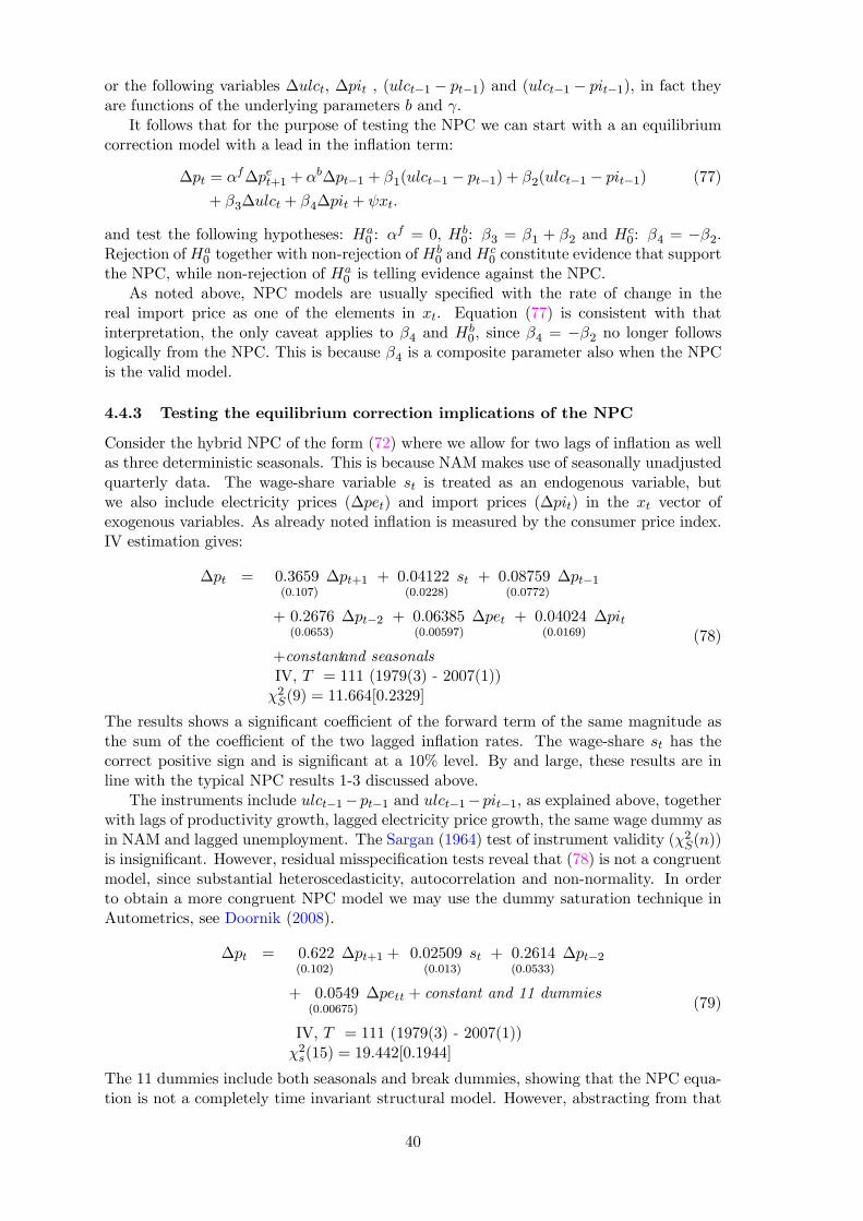
or the following variables ∆ulct, ∆pit , (ulct−1 − pt−1) and (ulct−1 − pit−1), in fact theyare functions of the underlying parameters b and γ.

It follows that for the purpose of testing the NPC we can start with a an equilibriumcorrection model with a lead in the inflation term:

∆pt = αf∆pet+1 + αb∆pt−1 + β1(ulct−1 − pt−1) + β2(ulct−1 − pit−1) (77)

+ β3∆ulct + β4∆pit + ψxt.

and test the following hypotheses: Ha0 : α

f = 0, Hb0: β3 = β1 + β2 and Hc

0: β4 = −β2.Rejection ofHa

0 together with non-rejection ofHb0 andH

c0 constitute evidence that support

the NPC, while non-rejection of Ha0 is telling evidence against the NPC.

As noted above, NPC models are usually specified with the rate of change in thereal import price as one of the elements in xt. Equation (77) is consistent with thatinterpretation, the only caveat applies to β4 and Hb

0, since β4 = −β2 no longer followslogically from the NPC. This is because β4 is a composite parameter also when the NPCis the valid model.

4.4.3 Testing the equilibrium correction implications of the NPC

Consider the hybrid NPC of the form (72) where we allow for two lags of inflation as wellas three deterministic seasonals. This is because NAM makes use of seasonally unadjustedquarterly data. The wage-share variable st is treated as an endogenous variable, butwe also include electricity prices (∆pet) and import prices (∆pit) in the xt vector ofexogenous variables. As already noted inflation is measured by the consumer price index.IV estimation gives:

∆pt = 0.3659(0.107)

∆pt+1 + 0.04122(0.0228)

st + 0.08759(0.0772)

∆pt−1

+ 0.2676(0.0653)

∆pt−2 + 0.06385(0.00597)

∆pet + 0.04024(0.0169)

∆pit

+constantand seasonalsIV, T = 111 (1979(3) - 2007(1))χ2S(9) = 11.664[0.2329]

(78)

The results shows a significant coefficient of the forward term of the same magnitude asthe sum of the coefficient of the two lagged inflation rates. The wage-share st has thecorrect positive sign and is significant at a 10% level. By and large, these results are inline with the typical NPC results 1-3 discussed above.

The instruments include ulct−1−pt−1 and ulct−1−pit−1, as explained above, togetherwith lags of productivity growth, lagged electricity price growth, the same wage dummy asin NAM and lagged unemployment. The Sargan (1964) test of instrument validity (χ2S(n))is insignificant. However, residual misspecification tests reveal that (78) is not a congruentmodel, since substantial heteroscedasticity, autocorrelation and non-normality. In orderto obtain a more congruent NPC model we may use the dummy saturation technique inAutometrics, see Doornik (2008).

∆pt = 0.622(0.102)

∆pt+1 + 0.02509(0.013)

st + 0.2614(0.0533)

∆pt−2

+ 0.0549(0.00675)

∆pett + constant and 11 dummies

IV, T = 111 (1979(3) - 2007(1))χ2s(15) = 19.442[0.1944]

(79)

The 11 dummies include both seasonals and break dummies, showing that the NPC equa-tion is not a completely time invariant structural model. However, abstracting from that

40

problem equation (79) is seen to adhere even closer to the stylized facts of the NPC thanequation (78).

As explained above, we want to test the hypothesis that (79) encompasses the priceequation of the incumbent model. To do that, we first include ulct−1 − pt−1 and ulct−1 −pit−1 as explanatory variables to obtain an empirical version of the embedding equation(77) above. We then do a general-to-specific search by means of autometrics in PcGive.The preferred model is reported as equation (80):

∆pt = 0.003849(0.069)

∆pt+1 + 0.08832(0.0259)

∆ulct + 0.1515(0.0577)

∆pt−2

+ 0.09883(0.0143)

(ulct−1 − pt−1)− 0.01943(0.00478)

(ulct−1 − pit−1) + 0.05164(0.00518)

∆pet

+Constant+ 4 dummiesIV, T = 111 (1979(3) - 2007(1))χ2S(16) = 25.434[0.0625]

(80)It is seen that the estimated forward coefficient αf is practically zero in (80) compared to0.62 in the NPC in (79). Hence the Hc

0: αf = 0 cannot be rejected statistically at any

meaningful level of significance.

4.5 Forecasting for monetary policy

A hallmark of modern and flexible inflation targeting is that the operational target variableis the forecasted rate of inflation, see i.e., Svensson (1997). One argument for this choiceof target is to be ahead of events, rather than to react after actual inflation has deviatedfrom target. In this way one may hope to achieve the target by a minimum of costs tothe real economy in terms of e.g., unwanted output fluctuations or large fluctuations inthe exchange rate. However, any inflation forecast is uncertain, and might induce wronguse of policy. Hence, a broad set of issues related to inflation forecasting is of interest forthose concerned with the operation and assessment of monetary policy.

A favourable starting point for inflation targeting is when it can be asserted thatthe central bank’s forecasting model is a good approximation to the inflation processin the economy. In this case, forecast uncertainty can be represented by conventionalforecast confidence intervals, or by the fan-charts used by today’s best practice inflationtargeters.20 The point of the probabilistic forecasts is to convey to the public that theforecasted inflation numbers only will coincide with the actual future rate of inflation onaverage, and that neighbouring inflation rates are almost as probable. By the same token,conditional on the forecasting model’s representation of uncertainty, still other inflationrates are seen to be wholly improbable realizations of the future.

However, the idea about model correctness and stationarity of macroeconomic processesis challenged by the high incidence of failures in economic forecasting, see e.g., Hendry(2001a). A characteristic of a forecast failure is that forecast errors turn out to be larger,and more systematic, than what is allowed if the model is correct in the first place. Inother words, realizations which the forecasts depict as highly unlikely (e.g., outside theconfidence interval computed from the uncertainties due to parameter estimation and lackof fit) have a tendency to materialize too frequently. Hence, as a description of real-lifeforecasting situations, an assumption about model correctness is untenable and representsa fragile foundation for forecast based interest rate setting, see Bårdsen et al. (2003).

20See e.g., Ericsson (2001) for a accessible discussion of forecast uncertainty, and its presentation inpublished forecasts.

41

4.5.1 Assumptions about the forecasting situation

In modern monetary policy the forecasted rate of inflation is the intermediate target. Itis then of interest to clarify as closely as possible what are the realistic properties of theforecast. Anticipated forecast properties are closely linked to the assumptions we makeabout the forecasting situation. An useful classification, see Clements and Hendry (1999,Ch 1), is:

A The forecasting model coincides with the true inflation process except for stochasticerror terms. The parameters of the model are known constants over the forecastingperiod.

B As in A, but the parameters have to be estimated.

C As in B, but we cannot expect the parameters to remain constant over the forecastingperiod–structural changes are likely to occur.

D We do not know how well the forecasting model correspond to the inflation mechanismin the forecast period.

A is an idealized description of the assumptions of macroeconomic forecasting. There is stillthe incumbency of inherent uncertainty represented by the stochastic disturbances–evenunder A. Situation B represents the situation theoretical expositions of inflation targetingconjure up, see Svensson (1999). The properties of situation A will still hold–even thoughthe inherent uncertainty will increase. If B represents the premise for actual inflationtargeting, there would be no forecast failures, defined as a significant deterioration offorecast performance relative to in-sample behaviour, see e.g. Hendry (2006). The within-sample-fit of section 4.2.2 above corresponds to situation B, subject to the assumptionthat NAM is a congruent model of the aggregate Norwegian economy.

The limited relevance of situation B for inflation targeting becomes clear once werecognize that in practice we do not know what kind of shocks that will hit the economyduring the forecast period. We generally refer to such changes as regime shifts, andtheir underlying causes include changes in technology and political decisions, and moregenerally, “the complexity and instability of human behaviour” (Elster (2007, p. 467)). Aforecast failure effectively invalidates any claim about a “correct” forecasting mechanism.Upon finding a forecast failure, the issue is therefore whether the misspecification wasdetectable or not, at the time of preparing the forecast. It is quite possible that a modelwhich has been thoroughly tested for misspecification within sample nevertheless forecastsbadly, which is a situation that may occur in situation C.

As discussed by Clements and Hendry (1999), a dominant source of forecast failureis regime shifts in the forecast period, i.e., after the preparation of the forecasts. Sincethere is no way of anticipating them, it is unavoidable that after forecast breaks damageforecasts from time to time. For example, when assessing inflation targeting over a periodof years, we anticipate that the forecasters have done markedly worse than they expectedat the time of preparing their forecasts, simply because there is no way of anticipatingstructural breaks before they occur. The task is then to be able to detect the nature of theregime shift as quickly as possible, in order to avoid repeated unnecessary forecast failure.

However, experience tells us that forecast failures are sometimes due to shocks andparameter changes that have taken place prior to the preparation of the forecast, butwhich have remained undetected by the forecasters. Failing to detect a before forecaststructural break might be due to low power of statistical tests of parameter instability.However, the power is actually quite high for the kind of breaks that are most damaging tomodel forecasts, see Hendry (2000). There are also practical circumstances that complicateand delay the detection of regime shifts. For example, there is usually uncertainty about

42

the quality of the provisional data for the period that initialize the forecasts, making itdifficult to assess the significance of a structural change or shock.

Hence both after and before forecast structural breaks are realistic aspects of reallife forecasting situations that deserve the attention of inflation targeters. In particular,one should seek forecasting models and tools which help cultivate an adaptive forecastingprocess. The literature on forecasting and model evaluation provide several guidelines, seee.g., Hendry (2001a) and Granger (1999).

Situation D brings us to the realistic situation, namely one of uncertainty and discordregarding what kind of model that approximates represents reality, in other words theissues of model specification and model evaluation. In section 4.3 we saw that in policyanalysis there is a clear gain from using the congruent model, and avoiding to base policyrecommendations on an misspecified model of the supply side. In forecasting, the linkbetween model misspecification and forecast failure is not always as straight-forward asone would first believe. The complicating factor is again non-stationarity, regime-shiftsand structural change. For example, a time series model in terms of the change in therate of inflation adapts quickly to changes in equilibria–a location shift– and is thereforerobust to before forecast structural breaks of this type, even though it clearly a misspec-ified model of the data generation process over the historical data period, see Clementsand Hendry (1999, Ch 5). Therefore a double differenced device (DDD) can deliver nearunbiased estimated when a location-shift have occurred prior to the preparation of theforecast. Conversely, a forecasting model of the equilibrium correction type is less adapt-able. Indeed, following an equilibrium shift, EqCM forecasts tend to move in the oppositeto the data, thereby causing forecast failure, cf. Hendry (2006). Eitrheim et al. (1999)showed that this new theory of forecasting has practical relevance for understanding theproperties of forecasts from an medium sized forecasting model of the Norwegian economy,in particular the more adaptive nature of DDD to several historical examples of structuralbreaks.

The new theory of forecasting that we build on does not deliver a carte blanche forusing non-congruent models for prediction, though. DDD and near equivalent forecastingdevices are robust for one particular reason: they do not equilibrium correct, and aretherefore insulated from changes in the parameters that are most pernicious for forecasting.Replacing a congruent and adequate EqCM with another, less adequate, EqCM model forforecasting is not a good idea. The non-congruent EqCM is also subject to forecast failureon its own premises, and without location shifts, it will forecast worse than the congruentEqCM. In this respect there is a cost to compromising model adequacy also in forecasting.In terms of the contesting supply-side models of section 4.3 this is illustrated by Bårdsenet al. (2002) who show that although the PCM is robust to some of the location shifts thatcan damage forecasting from the ICM, the cost of high forecast variance and bias due tomisspecified equilibrium correction dominates.

4.5.2 Real-time forecast performance

As mentioned above, NAM is part of the Normetrics system of models which was initiatedin 2005. Model based forecasts for the Norwegian economy are produced in January,March, June and September each year and published on the web. So far, these modelbased forecasts have performed relatively well compared to competing forecasts. As anexample Figure 9 shows forecasts for core inflation in 2006. Because of inflation targeting,this variable is the among the most thoroughly analyzed variable by both professionalforecasters both in the private and government sector.

43

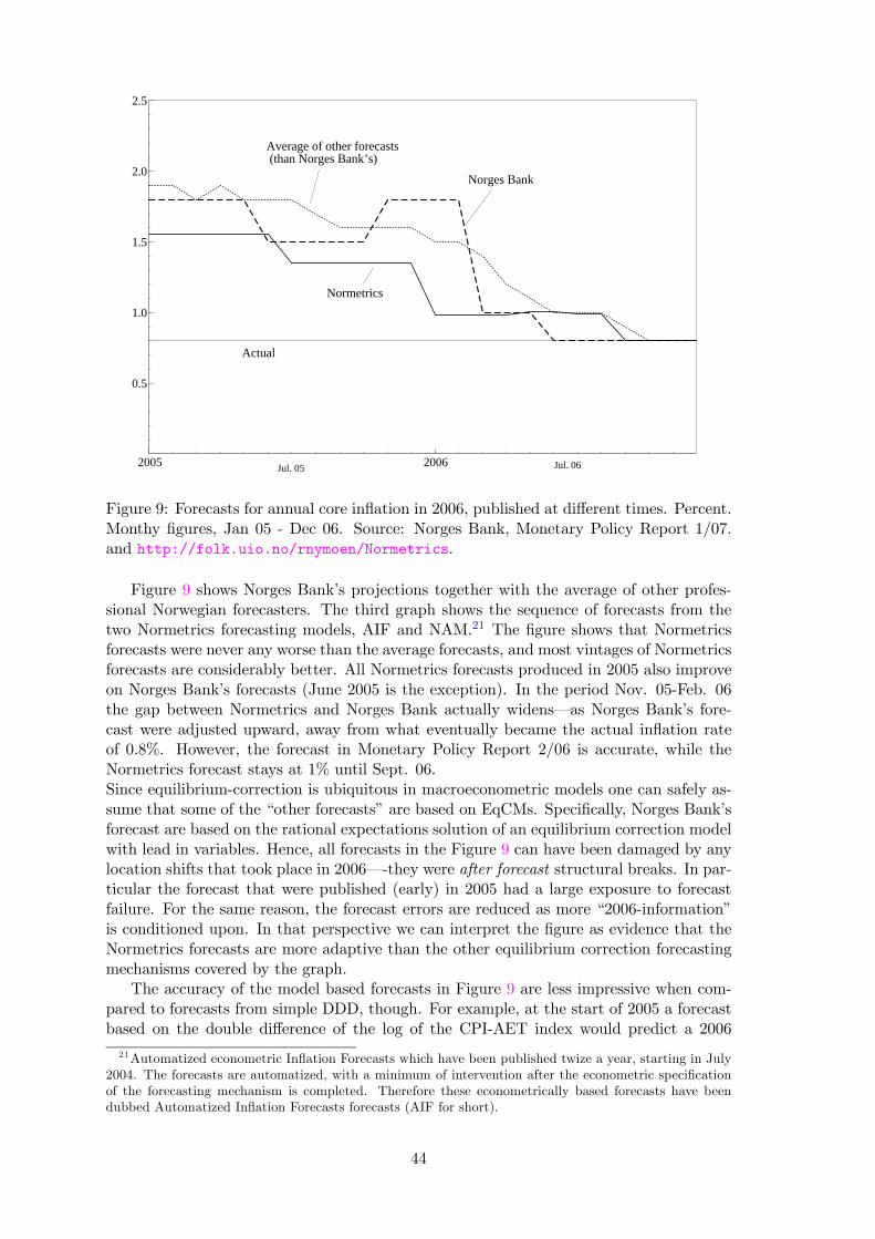
2005 2006

0.5

1.0

1.5

2.0

2.5

Jul. 05 Jul. 06

Norges Bank

Average of other forecasts (than Norges Bank’s)

Normetrics

Actual

Figure 9: Forecasts for annual core inflation in 2006, published at different times. Percent.Monthy figures, Jan 05 - Dec 06. Source: Norges Bank, Monetary Policy Report 1/07.and http://folk.uio.no/rnymoen/Normetrics.

Figure 9 shows Norges Bank’s projections together with the average of other profes-sional Norwegian forecasters. The third graph shows the sequence of forecasts from thetwo Normetrics forecasting models, AIF and NAM.21 The figure shows that Normetricsforecasts were never any worse than the average forecasts, and most vintages of Normetricsforecasts are considerably better. All Normetrics forecasts produced in 2005 also improveon Norges Bank’s forecasts (June 2005 is the exception). In the period Nov. 05-Feb. 06the gap between Normetrics and Norges Bank actually widens–as Norges Bank’s fore-cast were adjusted upward, away from what eventually became the actual inflation rateof 0.8%. However, the forecast in Monetary Policy Report 2/06 is accurate, while theNormetrics forecast stays at 1% until Sept. 06.Since equilibrium-correction is ubiquitous in macroeconometric models one can safely as-sume that some of the “other forecasts” are based on EqCMs. Specifically, Norges Bank’sforecast are based on the rational expectations solution of an equilibrium correction modelwith lead in variables. Hence, all forecasts in the Figure 9 can have been damaged by anylocation shifts that took place in 2006–-they were after forecast structural breaks. In par-ticular the forecast that were published (early) in 2005 had a large exposure to forecastfailure. For the same reason, the forecast errors are reduced as more “2006-information”is conditioned upon. In that perspective we can interpret the figure as evidence that theNormetrics forecasts are more adaptive than the other equilibrium correction forecastingmechanisms covered by the graph.

The accuracy of the model based forecasts in Figure 9 are less impressive when com-pared to forecasts from simple DDD, though. For example, at the start of 2005 a forecastbased on the double difference of the log of the CPI-AET index would predict a 2006

21Automatized econometric Inflation Forecasts which have been published twize a year, starting in July2004. The forecasts are automatized, with a minimum of intervention after the econometric specificationof the forecasting mechanism is completed. Therefore these econometrically based forecasts have beendubbed Automatized Inflation Forecasts forecasts (AIF for short).

44

inflation rate of 0.3%, which is a more accurate forecast than any of the econometric orprofessional forecasts that were produced in 2005. The DDD forecast is not improved onby Normetrics before January 2006, and not by Norges Bank before the Monetary PolicyReport 1/06 (from March). However, by this time also the DDD forecast could also behave been updated, most simply by replacing the 0.3% by the actual rate of inflation in2005 which was 1.0%. This forecast is practically identical to Normetrics forecasts frombefore September 2006, and it is not beaten by Norges Banks’ forecast before MPR 2/06.

The year 2006 is not the only one that the Normetrics forecasts compete well with theCentral Bank’s forecasts for the monetary policy target variable. Juel et al. (2008) notethat for a relatively long period of time, the automated forecasts from an empirically vali-dated inflation model, dubbed AIF above, have been better than Norges Bank’s forecasts.Figure 10 illustrates the point.

0 1 2 3 4 5 6 7 8 9 10 11

0.5

1.0

MSF

E

Length of forecast horizon (quarters)

Inflation Reports

AIF

0 1 2 3 4 5 6 7 8 9 10 11

−1.0

−0.5

0.0

MFE

Length of forecast horizon (quarters)

AIF

Inflation Reports

Figure 10: First panel: Mean forecast errors, MFE, for core inflation (annual rate ofchange in CPI-ATE). Inflation report forecasts and AIF forecasts. Second panel: Meansquared forecast errors, MSFE. Source: Inflation Report/Monetary Policy Report 2/04 -2/07 and AIFs published at http://folk.uio.no/rnymoen/forecast_air_index.html.

The figure can be used to assess the ex-ante forecasts based on forecast errors for theperiod 2004q2-2007q3. The forecasted variable is the annual rate of CPI-AET inflation.The graphs in the upper panel in the figure show the mean forecast errors, MFE. A negativeMFE means that the inflation forecasts are on average higher than the actual inflation ratesin the period. The biases of the econometric model (AIF) forecasts are small for forecasthorizons 1, 2, 3 and 4: the MFEs are less than 0.25 percentage points. Norges Bank’sinflation forecasts from the Inflation/Monetary Policy Reports are more biased than AIFfor horizons 2-8 quarters ahead. The biases of AIF become markedly bigger for forecastslength 7-10 quarters, and are not much different from the bias of forecasts produced byNorges Bank. The second panel of the figure shows the mean squared forecast errors,MSFE, to which large forecast errors contribute more than small errors. This measure

45

gives more or less the same picture at the mean forecast errors.

4.5.3 Ex post forecast evaluation and robustification.

The discussion of Figure 9 illustrates the general point that although EqCMs forecast wellwhen a process is difference-stationary, they are non-robust if there are non-stationaritiesdue to location shifts in the forecast period. In this particular case, the mean of the rateof inflation seems to have changed, in 2004 or earlier, and the DDD is a more adaptableforecasting mechanism than the EqCMs in the case of the before forecast structural break.The main benefit of DDDs for model based forecasting, where one wants to retain thecausal information of the model, is that DDDs can help the forecaster to robustify theEqCM forecasts by intercept corrections. The cost associated with DDDs is of coursethat the forecasts are more ‘noisy’ than EqCM forecasts, hence the forecast-error vari-ances associated with robust forecasts can become large, like when the first difference ofan autoregressive process doubles the 1-step forecast variance. In a model with one ortwo endogenous variables this cost may not be much of a issue, but in a multi-equationforecasting setting there may be a problem of extracting ‘signal from noise’ in practice. Inthe rest of this section we illustrate these issues by considering system forecasts.

-2

0

2

4

6

2003 2004 2005 2006 2007

a) Consumer price inf lation

1

2

3

4

5

2003 2004 2005 2006 2007

b) Unemployment rate

0

2

4

6

8

10

2003 2004 2005 2006 2007

c) Wage grow th

-5.0

-2.5

0.0

2.5

5.0

7.5

10.0

2003 2004 2005 2006 2007

d) GDP grow th

-8

-4

0

4

8

12

2003 2004 2005 2006 2007

e) Import price inf lation

80

85

90

95

100

105

110

2003 2004 2005 2006 2007

f) Real exchange rate

1

2

3

4

5

6

7

2003 2004 2005 2006 2007

g) Money market interest rate

0

4

8

12

16

2003 2004 2005 2006 2007

h) Real credit grow th

-20

-10

0

10

20

30

2003 2004 2005 2006 2007

i) Currency depreciation rate

Figure 11: Dynamic NAM forecasts 2003(1)-2007(3), with end-of-sample for estimation ofparameters in 2002(4). Actual values are shown by solid lines, and forecasts by dashedlines. The distance between the two dotted lines represents 70 % prediction intervals.

46

Figure 11 shows dynamic NAM forecasts for the period 2003(1)-2007(3).22 The sampleperiod for the estimation ends in 2002(4). Unlike the inflation forecasts in Figure 9, whichare real-time ex ante forecasts, we now consider ex post forecasts which are conditioned bythe true values of the non-modelled variables. Hence, the forecasts are not influenced bylocation shifts in the non-modelled variables (like foreign CPI inflation for example), butthey are subject to location shifts that are due to changes in the means of the estimatedcointegration relationships, or the autonomous growth rates (captured by intercepts aftersubtraction of equilibrium correction means).

Figure 11 serves as the reference case for discussion of the degree of adaptation of NAMforecasts, and for the properties of more robust forecasting devices that we investigate forcomparison. There are no less than five possible instances of location shifts in the forecastof these 9 variables. First, there is a systematic overprediction of the rate of inflation (weuse CPI inflation here) over the length of the forecast horizon. In the light of the 70%prediction interval, inflation overprediction is significant (forecast failure) in 2003. Second,unemployment is overpredicted and GDP growth in underpredicted for the 3 quarters of2007. Third, the short-term interest rate is significantly overpredicted in 2003(2)-2004(4).Fourth, real credit growth is underpredicted (significantly) from 2005(3). Finally, thereal exchange rate is systematically overpredicted from 2004(4) and onwards–the realappreciation of the Norwegian krone is not captured by the forecasts.

In the following we show how well the NAM forecasts adapt to these location shiftswhen we condition on 2004(4) and then 2006(4). In each dynamic forecast the coefficientestimate is updated. Figure 12 shows that the 2005(1)-2007(3) forecasts for inflation and,in particular, for the interest rate the real exchange rate have improved relative to Figure11. For the other variables there is little change, and if anything the forecast failures forthe rate of unemployment and for GDP growth stand out more clearly than before (alsoshowing that there is a knock-on effect of the high employment forecast on wage inflation).The explanation may be that NAM is unable to adapt, or that the location shifts of thevariables are of the after forecast also in this forecast.

22 In this section, we use the model version used for the October 2007 NAM forecasts, seehttp://folk.uio.no/rnymoen/namforecast_okt07.pdf

47

-2

0

2

4

6

2003 2004 2005 2006 2007

a) Consumer price inf lation

1.5

2.0

2.5

3.0

3.5

4.0

4.5

2003 2004 2005 2006 2007

b) Unemployment rate

1

2

3

4

5

6

7

2003 2004 2005 2006 2007

c) Wage grow th

-2

0

2

4

6

8

10

2003 2004 2005 2006 2007

d) GDP grow th

-4

-2

0

2

4

6

8

2003 2004 2005 2006 2007

e) Import price inf lation

84

88

92

96

100

104

2003 2004 2005 2006 2007

f) Real exchange rate

1

2

3

4

5

6

7

2003 2004 2005 2006 2007

g) Money market interest rate

0

4

8

12

16

2003 2004 2005 2006 2007

h) Real credit grow th

-10

-5

0

5

10

15

2003 2004 2005 2006 2007

i) Currency depreciation rate

Figure 12: Dynamic NAM forecasts 2005(1)-2007(3), with end-of-sample for estimation ofparameters in 2004(4). Actual values are shown by solid lines, and forecasts by dashedlines. The distance between the two dotted lines represents 70 % prediction intervals

Figure 13 focuses on the last three “problem variables” in terms of forecast failure. Therate of unemployment is now much better forecasted in 2007(1)-2007(3), which is a signof adaptation to a location shift which is of the before forecast category in this forecast,where 2006(4) is in the information set. For GDP and real credit growth the forecastfailures persist. In the present version of NAM, the high growth rates of 2007 can in partbe explained be the effects of very high oil prices on demand. In fact, that modellingdevice was used in Figure 6, showing the goodness-of-fit, but clearly would not be knownor of any help to a forecaster preparing forecast for 2007 late in the year of 2006.

48

1.5

2.0

2.5

3.0

3.5

4.0

4.5

2003 2004 2005 2006 2007

a) Unemployment rate

-2

0

2

4

6

8

10

2003 2004 2005 2006 2007

b) GDP grow th rate

0

4

8

12

16

2003 2004 2005 2006 2007

c) Real credit grow th

Figure 13: Dynamic NAM forecasts 2007(1)-2007(4), with end-of-sample for estimation ofparameters in 2006(4). Actual values are shown by solid lines, and forecasts by dashedlines. The distance between the two dotted lines represents 70 % prediction intervals

As mentioned above, using differencing (DDD above) to forecast provides more robustforecast when non-stationarities are due to location-shifts. As discussed by Hendry (2006),a differenced version of the EqCM may be interpreted as an augmented DDD forecastingrule. We therefore consider forecasts from the differenced NAM model, and refer to theseas dEqCM forecasts. In the differenced forecasting systems, some of the causal informationembedded in NAM is retained at the same time as the dEqCM has no constants neitherin the form of means of cointegration relationships or in the form of separate interceptterms, see Hendry (2006). Hence forecasts from the dEqCM does not equilibrium correct,thereby reducing the risks attached to EqCM forecasts.

49

-20

-10

0

10

20

2003 2004 2005 2006 2007

a) Consumer price inf lation

1

2

3

4

5

6

7

2003 2004 2005 2006 2007

b) Unemployment rate

-20

-10

0

10

20

30

2003 2004 2005 2006 2007

c) Wage grow th

-8

-4

0

4

8

12

2003 2004 2005 2006 2007

d) GDP grow th

-20

-10

0

10

20

30

2003 2004 2005 2006 2007

e) Import price inf lation

60

70

80

90

100

110

2003 2004 2005 2006 2007

f) Real exchange rate

-5

0

5

10

15

20

2003 2004 2005 2006 2007

g) Money market interest rate

-10

-5

0

5

10

15

2003 2004 2005 2006 2007

h) Real credit grow th

-20

-10

0

10

20

30

2003 2004 2005 2006 2007

i) Currency depreciation rate

Figure 14: Dynamic dEqCM forecasts 2003(1)-2007(3), with end-of-sample for estimationof parameters in 2002(4). Actual values are shown by solid lines, and forecasts by dashedlines. The distance between the two dotted lines represents 70 % prediction intervals

Figure 14 shows the dEqCM forecast for the 2003(1)-2007(3) period. Comparison withthe NAM forecasts in Figure 11 show that the increase in forecast variance is not a smallcost in this case–note the difference in scaling as well. The absolute forecast errors appearto be much worse than the NAM forecast errors as well. For example, unemploymentis predicted by the dEqCM to increase over the forecast horizon, and credit growth isunderpredicted for the length of the horizon.

Figure 15 shows the dEqCM forecasts when we condition on information including2004(4). Compared to the NAM forecasts that condition on the same information, seeFigure 12 there is little to be gain in these forecasts. We note that the dEqCM interestrate forecast has adapted, but the same happened with the NAM forecasts. The dEqCMforecasts are still uninformative about the behaviour of unemployment and credit growthover the 2006(1)-2007(3) period.

50

-8

-4

0

4

8

12

2003 2004 2005 2006 2007

a) Consumer price inf lation

1

2

3

4

5

6

7

2003 2004 2005 2006 2007

b) Unemployment rate

-15

-10

-5

0

5

10

15

2003 2004 2005 2006 2007

c) Wage grow th

-4

0

4

8

12

2003 2004 2005 2006 2007

d) GDP grow th

-10

-5

0

5

10

15

20

2003 2004 2005 2006 2007

e) Import price inf lation

75

80

85

90

95

100

105

2003 2004 2005 2006 2007

f) Real exchange rate

-4

0

4

8

12

2003 2004 2005 2006 2007

g) Money market interest rate

-5

0

5

10

15

20

2003 2004 2005 2006 2007

h) Real credit grow th

-15

-10

-5

0

5

10

15

2003 2004 2005 2006 2007

i) Currency depreciation rate

Figure 15: Dynamic dEqCM forecasts 2005(1)-2007(3), with end-of-sample for estimationof parameters in 2004(4). Actual values are shown by solid lines, and forecasts by dashedlines. The distance between the two dotted lines represents 70 % prediction intervals

1.5

2.0

2.5

3.0

3.5

4.0

4.5

2003 2004 2005 2006 2007

a) Unemployment rate

-2

0

2

4

6

8

10

2003 2004 2005 2006 2007

b) GDP grow th rate

0

4

8

12

16

2003 2004 2005 2006 2007

c) Real credit grow th

Figure 16: Dynamic dEqCM forecasts 2007(1)-2007(4), with end-of-sample for estimationof parameters in 2006(4) Actual values are shown by solid lines, and forecasts by dashedlines. The distance between the two dotted lines represents 70 % prediction intervals

Figure 16 indicates that for the three quarters of 2007, the dEqCM forecast for therate of unemployment is better than the (already quite good) NAM forecasts. However,for GDP growth and credit growth, the dEqCM still does not adjust to the location shift.

51

These results suggest that in practice, a more discretionary approach may be called for.For example, instead of taking away all the equilibrium correction by differencing, one mayconcentrate on the subset of equations which have failed because of location shifts in recentforecasting rounds, since that will induce lack of adaptation also in the overall forecastingpicture. To illustrate the possible benefit from such an approach, Figure 17 shows the2007 forecasts for a dEqCM where only the equilibrium variables of the aggregate demandand for the credit equation have been “differenced away”, to avoid confusion with thedEqCM used above, we refer to this forecasting model as partial-dEqCM. Figure 17 showsthe one-step forecast, since any differences in adaptability is then easier to see.

Panels a) and b) show the NAM forecasts. The forecasts for 2007(1) are the same asin Figure 16 for these two variables, but 2007(2) and 2007(2) are different since the NAMforecasts are now conditional on first and second quarter information for exogenous andpredetermined variables (the coefficients are not updated). The lack of adaptation to thelocation shifts of the growth rate of the actual series is apparent. Panel c) and d) showsthe corresponding partial-dEqCM forecasts. For GDP growth there is less underpredictionalready in 2007(1), and in 2007(2) the forecast has adapted. Panel c) shows a markedimprovement in adaptation also in the credit growth rate, although not before the secondquarter of 2007(2).

2006 2007 2008

2.5

5.0

7.5

10.0

NAM 1−step forecasts GDP growth

2006 2007 2008

10.0

12.5

15.0

NAM 1−step forecasts credit growth

2006 2007 2008

2.5

5.0

7.5

10.0

dECM 1−step forecasts GDP growth

2006 2007 2008

10.0

12.5

15.0

dECM 1−step forecasts credit growth

Figure 17: One-step forecast from NAM and a partial dEqCM. The forecasts are thedashed lines. The distance between the dotted lines represents 70 % prediction intervals

5 Conclusion

This chapter has presented a case for continuing to use macroeconometric models for policyanalysis, including such analyses that relies on instrument use to attain a certain forecastfor a target variable like inflation. Paradoxically, perhaps, the main line of argument startsfrom the recognition that accurate forecasting is a near impossibility in macroeconomics,because of the inherent non-stationarity of the economic time series included in the model

52

. Non-stationarity takes different forms, with different implications for macroeconomet-ric modelling and forecasting, and above we have distinguished between unit roots andnon-stationarity due to structural breaks. We have demonstrated that macroeconometricmodels can be developed theoretically and empirically in a way that is consistent with aunit root assumption. At the modelling and estimation stage, non-stationarity due to unitroots can principle be handled by cointegration methods, and, given that approach, unitroots are unlikely to be a source of forecast failures. On the contrary, a correct unit rootassumption can help in concentrating on predictable functions of variables, like growthrates and linear combination of target variables.

Non-stationarity due to structural breaks in functional relationships of the economyseem to represent the real challenge to macroeconometric modelling. Structural breaks inthe forecast period are particularly harmful since they are untraceable and will make themodel forecasts go toward pre-break steady-state relationships. When the sample periodis extended, structural breaks represent valuable sample information that provide powerto tests of economic hypotheses, and in that perspective structural breaks are seen to benot entirely negative since there can be progress in macroeconometric modelling throughforecast failure.

It follows from our approach that we agree with those who conclude that guidancefrom economic theory is important in the forecasting process, cf. Elliott and Timmermann(2008). But theory and modern econometrics do not provide immunity to new structuralbreaks. Nevertheless, the case for macroeconometric system of equations models may toa large extent depend of their ability to forecast relatively well compared to competingforecasting methods. Making models sufficiently adaptive to a structural break once theevidence is there that it has occurred is a necessary step in that project.

It is possible to look to other forecasting disciplines for inspiration. Meteorologists de-veloped their forecasting theory, models and routines between the two world wars. Thoseforecast were based on a deterministic model of the dynamics of the atmosphere. Then,in the mid-sixties, the understanding of the dynamics were completely altered with thedevelopment and acceptance of chaos theory, with the logical consequence that accurateweather forecast is impossible. Thirty years after the arrival of the meteorologists ’impos-sibility theory’ for forecasting, the weather forecasts are undeniably more accurate thanever. Hence, the weather is predictable even 10 days ahead, despite the chaos representedby the underlying forecasting models. It is perhaps unlikely that we will witness somethingsimilar in economics, but there are nevertheless parallels. Meteorologists have precise the-ory and almost continuous updating of initial conditions. Policy oriented modelling mayhave to live with idealized or partial theories, and with variables that are measured atrelatively long time intervals, and which are influenced by measurement errors. Yet, as adiscipline we have developed methods and strategies that are quite good at making themost of ‘small data amounts’. Hence while meteorologists can rely on the theoreticallyspecified model of weather dynamics, the interaction between economic theory, economet-ric theory, good model selection procedures, and diagnostic testing have together greatlyimproved our capability of modelling the macro economy, thus providing models that canaid policy decisions.

A Data definitions and equation statistics

A.1 Variables

TThe model employs seasonally unadjusted data. Unless another source is given, all dataare taken from FPAS, the database of Norges Bank.

The model is developed and estimated with Oxmetrics 5 (www.oxmetrics.net) andthen reestimated and simulated with Eviews 6 ( www.eviews.com).

53

V Trade weighted nominal value of the krone based on import-shares of trading countries.

G Government sector consumption expenditure, fixed 1991 prices. Mill. NOK.

L Nominal credit volume. Mill. NOK.

R Money market interest rate (3 month Euro-krone interest rate).

R∗ ECU interest rate. For the period 1967(1)-1986(3): Effective interest rate on for-eign bonds, NOK-basket weighted. For the period 1986(4)-1996(4): ECU weightedeffective rate on foreign bonds.

RL Average interest rate on bank loans.

RB Yield on 6 years government bond, quarterly average.

R∗B Yield on long term foreign bonds. NOK basket weighted.

P Consumer price index (CPI).

PC "Core" consumer price index.

P ∗ Consumer prices abroad in foreign currency.

PE CPI, electricity, fuel and lubricants.

PO USD oil price, per barrel Brent-Blend.

PI Price deflator of total imports.

P ∗I Producer price index, trading partners.

Y Total value added at market prices in the mainland economy (defined as total economyminus North-Sea oil and gas production and international shipping). Fixed baseyear (1991) prices. Mill. NOK.

Z Mainland economy value added per man hour at factor costs.

T1 Payroll tax rate, mainland economy.

U Registered rate of unemployment.

W Nominal hourly wage COSTS in the mainland economy. NOK.

In addition, there is a step dummy, accounting for the introduction of inflation target-ing.

IT = 0 until 2001(1), 1 from 2001(2)

A.2 Notation for estimation and mispecification tests

In Table 1 and 2, the estimation method, which is either ordinary least squares (OLS),or full information maximum likelihood (FIML) is indicated in the first line below eachequation, along with the sample size (number of quarterly observations) which is denotedby T , and the residual standard error (σ). For equations estimated with OLS, statis-tics for residual autocorrelation and ARCH form heteroscedasticity are reported in thesecond line below the equation. As indicated by the notation, these two statistics areF-distributed under their respective null hypotheses. For example, FAR(1−4)(4, 44) in theexchange rate equation denotes the F distributed test statistics with 4 and 44 degrees offreedom for the null hypothesis of no autocorrelation against the alternative of 4th order

54

autoregressive autocorrelation. In the third line below the estimated OLS equations, wereport the Chi-square distributed test of residual normality, and the F distributed testof heteroscedasticity due to squares of the regressors. For the equations estimated withFIML, systems versions of the misspecification tests are reported and are indicated by theextra subscript vec, as Fvec,AR(1−4). The numbers in brackets are p-values for the respec-tive null hypotheses These, as well as the other standard diagnostics tests, are explainedin Doornik and Hendry (2007a) (single equation diagnostics), or Doornik and Hendry(2007b) (system and simultaneous equations diagnostics).

References

Akram, Q. (2007). Designing Monetary Policy Using Econometric Models,. Norges Bank,Oslo.

Akram, Q. F. and R. Nymoen (2008). Model Selection for Monetary Policy Analysis–How Important is Empirical Validity? Oxford Bulletin of Economics and Statistics, 70 .Forthcoming.

Aldrich, J. (1989). Autonomy. Oxford Economic Papers, 41 , 15—34.

Andersen, T. M. (1994). Price Rigidity. Causes and Macroeconomic Implications. Clare-don Press, Oxford.

Ball, L. (1999). Policy Rules for Open Economies. In Taylor, J. B. (ed.), MonetaryPolicy Rules, A National Bureau of Economic Research Conference Report, 127—144.University of Chicago Press, Chicago.

Bårdsen, G., Ø. Eitrheim, E. S. Jansen and R. Nymoen (2005). The Econometrics ofMacroeconomic Modelling . Oxford University Press, Oxford.

Bårdsen, G. and P. G. Fisher (1993). The Importance of Being Structured. Discussionpaper 02/93, Institute of Economics, Norwegian School of Economics and BusinessAdministration.

Bårdsen, G. and P. G. Fisher (1999). Economic Theory and Econometric Dynamics inModelling Wages and Prices in the United Kingdom. Empirical Economics, 24 (3),483—507.

Bårdsen, G., P. G. Fisher and R. Nymoen (1998a). Business Cycles: Real Facts or Fal-lacies? In Strøm, S. (ed.), Econometrics and Economic Theory in the 20th Century:The Ragnar Frisch Centennial Symposium, no. 32 in Econometric Society MonographSeries, chap. 16, 499—527. Cambridge University Press, Cambridge.

Bårdsen, G., P. G. Fisher and R. Nymoen (1998b). Business Cycles: Real Facts or Fal-lacies? In Strøm, S. (ed.), Econometrics and Economic Theory in the 20th Century:The Ragnar Frisch Centennial Symposium, no. 32 in Econometric Society MonographSeries, chap. 16, 499—527. Cambridge University Press, Cambridge. Econometric SocietyMonographs No. 31.

Bårdsen, G., S. Hurn and K. Lindsay (2004a). Linearizations and equilibrium correctionmodels. Studies in Nonlinear Dynamics and Econometrics , 8 (5).

Bårdsen, G., E. S. Jansen and R. Nymoen (2002). Model Specification and InflationForecast Uncertainty. Annales d’économie et de Statistique, 67 (68), 495—517.

Bårdsen, G., E. S. Jansen and R. Nymoen (2003). Econometric Inflation Targeting. Econo-metrics Journal , 6 (2), 429—460.

55

Bårdsen, G., E. S. Jansen and R. Nymoen (2004b). Econometric Evaluation of the NewKeynesian Phillips Curve. Oxford Bulletin of Economics and Statistics, 66 (s1), 671—686.

Bårdsen, G. and J. T. Klovland (2000). Shaken or Stirred? Financial Deregulation andthe Monetary Transmission Mechanism in Norway. Scandinavian Journal of Economics,102 (4), 563—583.

Bårdsen, G. and R. Nymoen (2001). Rente Og Inflasjon (Interest Rate and Inflation).Norsk Økonomisk Tidsskrift , 115 , 125—48.

Bårdsen, G. and R. Nymoen (2003). Testing Steady-State Implications for the NAIRU.Review of Economics and Statistics, 85 , 1070–1075.

Bårdsen, G. and R. Nymoen (2009). U.S. Natural Rate Dynamics Reconsidered. In Castle,J. and N. Shephard (eds.), The Methodology and Practise of Econometrics, chap. 16,389—414. Oxford University Press, Oxford.

Barkbu, B. B., R. Nymoen and K. Røed (2003). Wage Coordination and UnemploymentDynamics in Norway and Sweden. Journal of Socio-Economics, 32 , 37—58.

Batini, N., B. Jackson and S. Nickell (2005). An Open-Economy New Keynesian PhillipsCurve for the U.K. Journal of Monetary Economics, 52 , 1061–1071.

Bjørnstad, R. and R. Nymoen (2006). The New Keynesian Phillips Curve Testes on OECDPanel Data. Mimeo, Department of Economics, University of Oslo.

Blanchard, O. J. and L. Katz (1999). Wage Dynamics: Reconciling Theory and Evidence.American Economic Review , 89 (2), 69—74. Papers and Proceedings (May, 1999).

Blanchflower, D. G. and A. J. Oswald (1994). The Wage Curve. The MIT Press, Cam-bridge, Massachusetts.

Calmfors, L. and R. Nymoen (1990). Nordic Employment. Economic Policy, 5 (11), 397—448.

Campbell, J. (1994). Inspecting the mechanism: an analytical approach to the stochasticgrowth model. Journal of Monetary Economics , 33 (3), 463—506.

Clarida, R., J. Gali and M. Gertler (1999). The Science of Monetary Policy: A NewKeynesian Perspective. Journal of Economic Literature, 37 (4), 1661—1707.

Clements, M. P. and D. F. Hendry (1999). Forecasting Non-stationary Economic TimeSeries. The MIT Press, Cambridge, MA.

Doornik, J. and D. H. Hendry (2007a). Empirical Econometric Modelling. PcGive 12.,vol. 1. Timberlake Consultants LTD, London.

Doornik, J. and D. H. Hendry (2007b). Modelling Dynamic Systems. PcGive 12., vol. 2.Timberlake Consultants LTD, London.

Doornik, J. A. (2008). Autometrics. In Castle, J. L. and N. shephard (eds.), The Method-ology and Practise of Econometrics. Oxford University Press.

Doornik, J. A. and D. F. Hendry (1997). The Implications for Econometric Modelling ofForecast Failure. Scottish Journal of Political Economy , 44 , 437—461.

Eitrheim, Ø., T. A. Husebø and R. Nymoen (1999). Equilibrium-Correction versus Dif-ferencing in Macroeconomic Forecasting. Economic Modelling , 16 , 515—544.

56

Eitrheim, Ø., E. S. Jansen and R. Nymoen (2002). Progress from Forecast Failure: TheNorwegian Consumption Function. Econometrics Journal , 5 , 40—64.

Elliott, G. and A. Timmermann (2008). Economic Forecasting. Journal of EconomicLiterature, 46 , 3–56.

Elster, J. (2007). Explaining Social Behaviour. More Nuts and Bolts for the Social Sci-ences. Cambridge University Press, Cambridge.

Engle, R. F. and D. F. Hendry (1993). Testing Super Exogeneity and Invariance inRegression Equations. Journal of Econometrics, 56 , 119—139.

Ericsson, N. R. (2001). Forecast Uncertainty in Economic Modeling. In Hendry, D. F. andN. R. Ericsson (eds.), Understanding Economic Forecasts, chap. 5, 68–92. The MITPress, Cambridge, Massachusetts.

Ericsson, N. R. and D. Hendry (1999). Encompassing and Rational Expectations: HowSequential Corroboration Can Imply Refutation. Empirical Economics, 24 (1), 1–21.

Ericsson, N. R. and J. S. Irons (1995). The Lucas Critique in Practice: Theory WithoutMeasurement. In Hoover, K. D. (ed.), Macroeconometrics: Developments, Tensions andProspects, chap. 8. Kluwer Academic Publishers.

Fanelli, L. (2007). Testing the New Keynesian Phillips Curve Through Vector Autoregres-sive Models: Results from the Euro Area. Forthcoming in Oxford Bulletin of Economicsand Statistics.

Frisch, R. (1936). On the Notion of Equilibrium and Disequilibrium. The Review ofEconomic Studies, 3 , 100–105.

Fuhrer, J. (2006). Intrinsic and Inherited Inflation Persistence. International Journal ofCentral Banking , 2 , 49–86.

Gali, J. and M. Gertler (1999). Inflation Dynamics: A Structural Econometric Analysis.Journal of Monetary Economics, 44 (2), 233—258.

Gali, J., M. Gertler and D. López-Salido (2001). European Inflation Dynamics. EuropeanEconomic Review , 45 , 1237—1270.

Gali, J., M. Gertler and J. Lopez-Salido (2005). Robustness of the Estimates of the HybridNew Keynesian Phillips Curve. Journal of Monetary Economics, 52 , 1107–1118.

Garratt, A., K. Lee, M. H. Pesaran and Y. Shin (2006). Global and National Macroecono-metric Modelling: A Long-Run Structural Approach. Oxford University Press.

Granger, C. W. J. (1992). Fellow’s Opinion: Evaluating Economic Theory. Journal ofEconometrics, 51 , 3–5.

Granger, C. W. J. (1999). Empirical Modeling in Economics. Specification and Evaluation.Cambridge University Press, Cambridge.

Haavelmo, T. (1944). The Probability Approach in Econometrics. Econometrica, 12 ,1—118. Supplement.

Hahn, F. and R. Solow (1997). A Critical Essay on Modern Macroeconomic Theory . MITPress, Cambridge.

Hendry, D. (2004). Robustifying Forecasts from Equilibrium-Correction Models. NuffieldCollege. Oxford University.

57

Hendry, D. (2006). Robustifying Forecasts from Equilibrium-Correction Systems. Journalof Econometrics, 135 , 399–426.

Hendry, D. F. (1988). The Encompassing Implications of Feedback versus FeedforwardMechanisms in Econometrics. Oxford Economic Papers, 40 , 132—149.

Hendry, D. F. (1995a). Dynamic Econometrics. Oxford University Press, Oxford.

Hendry, D. F. (1995b). Econometrics and business cycle empirics. Economic Journal ,105 , 1622—1636.

Hendry, D. F. (2000). On Detectable and Non-detectable Structural Change. StructuralChange and Economic Dynamics, 11 , 45—65.

Hendry, D. F. (2001a). How Economists Forecast. In Ericsson, N. R. and D. F. Hendry(eds.), Understanding Economic Forecasts , chap. 2, 15–41. The MIT Press, Cambridge,Massachusetts.

Hendry, D. F. (2001b). Modelling UK inflation. Journal of Applied Econometrics , 16 ,255—275.

Hendry, D. F. and H. M. Krolzig (1999). Improving on "Data Mining Reconsidered" byK.D. Hoover and S.J. Perez. Econometrics Journal , 2 , 41—58.

Hendry, D. F. and G. E. Mizon (2000). Reformulating Empirical Macroeconometric Mod-elling. Oxford Review of Economic Policy, 16 (4), 138–157.

Hoover, K. D. and S. J. Perez (1999). Data Mining Reconsidered: Encompassing and theGeneral-to-Spesific Approach to Specification Search. Econometrics Journal , 2 , 1—25.

Johansen, L. (1977). Lectures on Macroeconomic Planning. Volume 1. general aspects.North-Holland, Amsterdam.

Johansen, S. (1995). Likelihood-Based Inference in Cointegrated Vector AutoregressiveModels . Oxford University Press, Oxford.

Johansen, S. (2006). Cointegration: An Overview. In Mills, T. C. and K. Patterson (eds.),Palgrave Handbook of Econometrics , vol. 1 of Econometric Theory. Palgrave-MacMillan.

Johansen, S. and A. R. Swensen (1999). Testing exact rational expectations in cointegratedvector autoregressive models. Journal of Econometrics, 93 , 73—91.

Johansen, S. and A. R. Swensen (2004). More on testing exact rational expectations incointegrated vector autoregressive models: Restricted constant and linear term. Econo-metrics Journal , 7 , 389—397.

Juel, S., K. Molnar and K. Røed (2008). Norges Bank Watch 2008. An Independent Reviewof Monetary Policymaking in Norway. Tech. rep., Centre for Monetary Economics atthe Norwegian School of Management, BI. Http://www.bi.no/cmeFiles/NBW2008

Juselius, K. (2007). The Cointegrated VAR Model: Methodology and Applications. OxfordUniversity Press.

Kolsrud, D. and R. Nymoen (1998). Unemployment and the Open Economy Wage-PriceSpiral. Journal of Economic Studies, 25 , 450—467.

Layard, R., S. Nickell and R. Jackman (1991). Unemployment . Oxford University Press,Oxford.

58

Layard, R., S. Nickell and R. Jackman (1994). The Unemployment Crisis. Oxford Uni-versity Press, Oxford.

Layard, R., S. Nickell and R. Jackman (2005). Unemployment . Oxford University Press,Oxford, 2nd edn.

Lucas, R. E. J. (1976). Econometric Policy Evaluation: A Critique. In Brunner, K.and A. M. Meltzer (eds.), The Phillips Curve and Labour Markets, 19—46. Carnegie-Rochester Conference on Public Policy, 3.

Lütkepohl, H. (2006). Vector Autoregressive Models. In Mills, T. C. and K. Patterson(eds.), Econometric Theory, vol. 1 of Palgrave Handbook of Econometrics, 287—325.Palgrave MacMillan.

Mavroeidis, S. (2006). Testing the New Keynesian Phillips Curve Without AssumingIdentification. Brown Economic Papers 2006-13. Brown Universiy.

Nymoen, R. (1991a). A small linear model of wage- and price-inflation in the Norwegianeconomy. Journal of Applied Econometrics, 6 , 255—69.

Nymoen, R. (1991b). A Small Linear Model of Wage- and Price-Inflation in the NorwegianEconomy. Journal of Applied Econometrics, 6 , 255—269.

Nymoen, R. (2005). Evaluating a Central Bank’s Recent Forecast Failure. Memorandum22/05, Department of Economics, University of Oslo.

Nymoen, R. and A. Rødseth (2003). Explaining Unemployment: Some Lessons fromNordic Wage Formation. Labour Economics, 10 , 1–29.

Pagan, A. (2003). Report on modeling and forecasting at the Bank of England. Bank ofEngland Quarterly Bulletin, 60—88.

Patterson, K. D. (1987). Growth Coefficients in Dynamic Time Series Models. OxfordEconomic Papers, 39 (2), 282—292.

Patterson, K. D. and Ryding, J. (1984). Dynamic Time Series Models with Growth EffectsConstrained to Zero. The Economic Journal , 94 (373), 137—143.

Pesaran, M. H. and R. P. Smith (1985). Evaluation of Macroeconomic Models. EconomicModelling , 125–134.

Rudd, J. and K. Whelan (2005). Does Labor’s Share Drive Inflation? Journal of Creditand Banking , 37 (2), 297–312.

Rudd, J. and K. Whelan (2007). Modeling Inflation Dynamics: A Critical Review ofRecent Work. Journal of Credit and Banking , 39 (2), 155–170.

Sargan, J. D. (1964). Wages and Prices in the United Kingdom: A Study of EconometricMethodology. In Hart, P. E., G. Mills and J. K. Whitaker (eds.), Econometric Analysisfor National Economic Planning , 25—63. Butterworth Co., London.

Sargan, J. D. (1980). A Model of Wage-Price Inflation. Review of Economic Studies, 47 ,113—135.

Spanos, A. (2006). Econometrics in Retrospect and Prospect. In Mills, C. and K. Patterson(eds.), Palgrave Handbook of Econometrics. Volume 1. Econometric Theory , vol. 1,chap. 1, 3–58. Palgrave Macmillan, Houndsmills, New York.

59

Spanos, A. (2008). Suffiency and Acillarity Revisited: Testing the Validity of a StatisticalModel. In Castle, J. L. and N. Shephard (eds.), The Methodology and Practice ofEconometrics. Oxford Univeristy Press, Oxford.

Stanley, T. D. (2000). An Empirical Critique of the Lucas Critique. Journal of Socio-Economics, 29 , 91—107.

Svensson, L. (1997). Inflation Forecast Targeting: Implementing and Monitoring InflationTargets. European Economic Review , 41 , 1111—1146.

Svensson, L. (1999). Inflation Targeting: Some Extensions. Scandinavian Journal ofEconomics, 101 (3), 337–361.

Uhlig, H. (1999). A toolkit for analysing nonlinear dynamic stochastic models easily. InMarimon, R. and A. Scott (eds.), Computational Methods for the Study of DynamicEconomies, 30—61. Oxford University Press, Oxford.

60