Testing Structural Stability

in Macroeconometric Models1

Otilia BoldeaTilburg University

and

Alastair R. Hall2

University of Manchester

December 6, 2011

1This manuscript is prepared for Handbook of Research Methods and Applicationson Empirical Macroeconomics edited by N. Hashimzade and M. Thornton which is tobe published by Edward Elgar. The second author acknowledges the support of theESRC grant RES-062-23-1351. We thank Denise Osborn for useful conversations inthe preparation of this manuscript.

2Corresponding author. Economics, SoSS, University of Manchester, ManchesterM13 9PL, UK. Email: alastair.hall@manchester.ac.uk

1 Introduction

Since the earliest days of macroeconometric analysis, researchers have been con-cerned about the appropriateness of the assumption that model parameters re-main constant over long periods of time; for example see Tinbergen (1939).1

This concern is also central to the so-called the Lucas (1976) critique which hasplayed a central role in shaping macroeconometric analysis in the last thirtyyears. Lucas (1976) emphasizes the fact that the decision models of economicagents are hard to describe in terms of stable parametrizations, simply be-cause changes in policy may change these decision models and their respectiveparametrization. These arguments underscore the importance of using struc-tural stability tests as diagnostic checks for macroeconometric models.

A large body of empirical macroeconomic studies provides evidence for pa-rameter instability in a variety of macroeconomic models. For example, consid-erable evidence exists that the New Keynesian Phillips curve has become flatand/or less persistent in recent years - see e.g. Alogoskoufis and Smith (1991),Cogley and Sargent (2001), Zhang, Osborn, and Kim (2008), Kang, Kim, andMorley (2009). Similarly, there is evidence that the interest rate reaction func-tion is asymmetric over the business cycle - see e.g. Boivin and Giannoni (2006),Surico (2007), Benati and Surico (2008), Liu, Waggoner, and Zha (2009). Ex-amples of parameter instability are not confined to monetary policy, but alsoextend to: growth models - Ben-David, Lumsdaine, and Papell (2003); outputmodels - Perron (1997), Hansen (1992); exchange rate models - Rossi (2006); un-employment rate models - Weber (1995), Papell, Murray, and Ghiblawi (2000),Hansen (1997b), and many more. If such instabilities are ignored in the esti-mation procedure, they lead to incorrect policy recommendations and flawedmacroeconomic forecasts.

Thus, it is essential - and it has become common practice - to test for in-stability in macroeconomic models. Instabilities can be of many types. In thischapter, we describe econometric tests for three main types of instability: pa-rameter breaks, other parameter instabilities and model instabilities.

The first category, parameter breaks, focuses on sudden parameter changes.It may be desired to test for change that occurs at a particular time. In thiscase, the time of change, called break-point in econometrics and change-pointin statistics, is said to be known. It can also be that it is desired to test forchange at some unspecified point in the sample. In this case, the break-pointis said to be unknown. We discuss tests for both a known and an unknownbreak. We also present methods for detecting multiple break-points, and theirpractical implementation.

For the second category, other parameter instabilities, we give a brief butthorough account of the state of the art tests for threshold models, smoothtransition models and Markov-switching models.

In practice, there is no reason to assume that only parameters change, whilethe underlying functional form stays the same. Therefore, the third category

1See Morgan (1990) for review of Tinbergen’s contributions.

1

of tests we describe is for model instabilities, when the functional form of themodel is allowed to change after a known or unknown break.

In macroeconomics, the tests we present are often viewed as tests for Lucascritique. Lucas critique, at the time it was written, was directed against the useof backward-looking expectations, which did not take into account that agentswill change their decision making when policy changes occur, leading to pa-rameter or model instability. However, as Estrella and Fuhrer (2003) point out,using forward-looking expectations that incorporate certain policy changes doesnot make a model immune either to Lucas critique or to parameter or modelinstability. To see this, note that even if a structural model of the economyexists - with forward-looking behavior, based on solid microeconomic founda-tions, with important policy functions specified - it is unclear one can derivethe complete model, or estimate it in practice. Any simplification, parametercalibration, omission or misspecification of relevant policy functions and otheragent decisions can lead to parameter or model instability. Thus, even though itis often stated that Lucas critique implies that only reduced-form models sufferfrom instability - see e.g. Lubik and Surico (2010), in practice all models areprone to this problem and need to be tested for instability.2

In this chapter, we discuss Wald-type tests for breaks that are based onleast-squares (LS) type methods, suitable for reduced-form models, and alsoon two-stage least-squares (2SLS) and generalized method of moments (GMM)estimation, more suitable for structural models. The chapter is organized asfollows. In Section 2, we present structural stability tests for a single break basedon GMM estimation. In Section 3, we discuss testing strategies for multiplebreak-points. Section 4 provides an brief but thorough account of tests for othertypes of parameter instability, with comments on the most recent developmentsin this literature. Section 5 focuses on testing for model instabilities rather thanparameter instabilities. Section 6 concludes.

2 Testing for discrete parameter change at a sin-

gle point

In this section, we summarize the literature on testing for discrete parameterchange in macroeconometric models based on GMM. GMM provides a methodfor estimation of the parameters of a macroeconomic model based on the infor-mation in a population moment condition. GMM is described elsewhere in thisvolume, see Chapter 14, and so here we assume knowledge of the basic GMMframework. For ease of reference, we adopt the same generic notation as in Hall

2The name “structural instability” refers to the economic structure being unstable, encom-

passing instability in both structural and reduced-form models.

2

(2011): thus, the population moment condition is written as E[f(vt, θ0)] = 0 inwhich θ0 denotes the true value of the p × 1 parameter, vt is a random vector,and f( · ) is a q × 1 vector of continuous differentiable functions.3 The sampleis assumed to consist of observations on {vt, t = 1, 2, . . .T}.

As befits the GMM framework, the null and alternative hypotheses are ex-pressed in terms of the population moment condition. The null hypothesisis that the population moment condition holds at the same parameter valuethroughout the sample. The alternative of interest here is that the populationmoment condition holds at one value of the parameters up until a particularpoint in the sample, called break-point, after which the population momentcondition holds at a different parameter value. To formally present the hy-potheses of interest here, we need a notation for the break-point. Following theconvention in the literature, we let λ be a constant defined on (0, 1) and let [Tλ]denote the potential break-point at which some aspect of the model changes.4

For our purposes here, it is convenient to divide the original sample into twosub–samples. Sub–sample 1 consists of the observations before the break-point,namely T1(λ) = {1, 2, . . . , [λT ]}, and sub–sample 2 consists of the observationsafter the break-point, T2(λ) = {[λT ] + 1, . . .T}.

As mentioned in the introduction, this break-point may be treated as knownor unknown in the construction of the tests. If it is known, then the break-pointis specified a priori by the researcher and it is only desired to test for instabilityat this point alone. For example, Clarida, Gali, and Gertler (2000) investigatewhether the monetary policy reaction function of the Federal Reserve Board isdifferent during the tenure of different chairmen. Of particular interest in theirstudy is whether or not the the reaction function is different pre- and post-1979,the year Paul Volcker was appointed as Chairman. Since their analysis usesquarterly data, this involves exploring whether or not there is parameter changeat the fixed break date with [Tλ] = 1979.2. If the break-point is unknown, thealternative is the broader hypothesis that there is parameter change at somepoint in the sample. We begin our discussion with the simpler case in which thebreak-point is known, and then consider the extension to the unknown break-point case.

For a fixed break-point indexed by λ, the null hypothesis of interest can beexpressed mathematically as,

H0 : E[f(vt, θ0)] = 0, for t = 1, 2, . . ., T, (1)

and the alternative hypothesis as,

H1(λ) : E[f(vt, θ1)] = 0, for t ∈ T1(λ)E[f(vt, θ2)] = 0, for t ∈ T2(λ),

where θ1 6= θ2.3We adopt the convention of using “0” to denote either a scalar, vector or matrix of zero(s)

with the dimension determined by the term on the other side of the equation.4Here, [·] stands for the integer part.

3

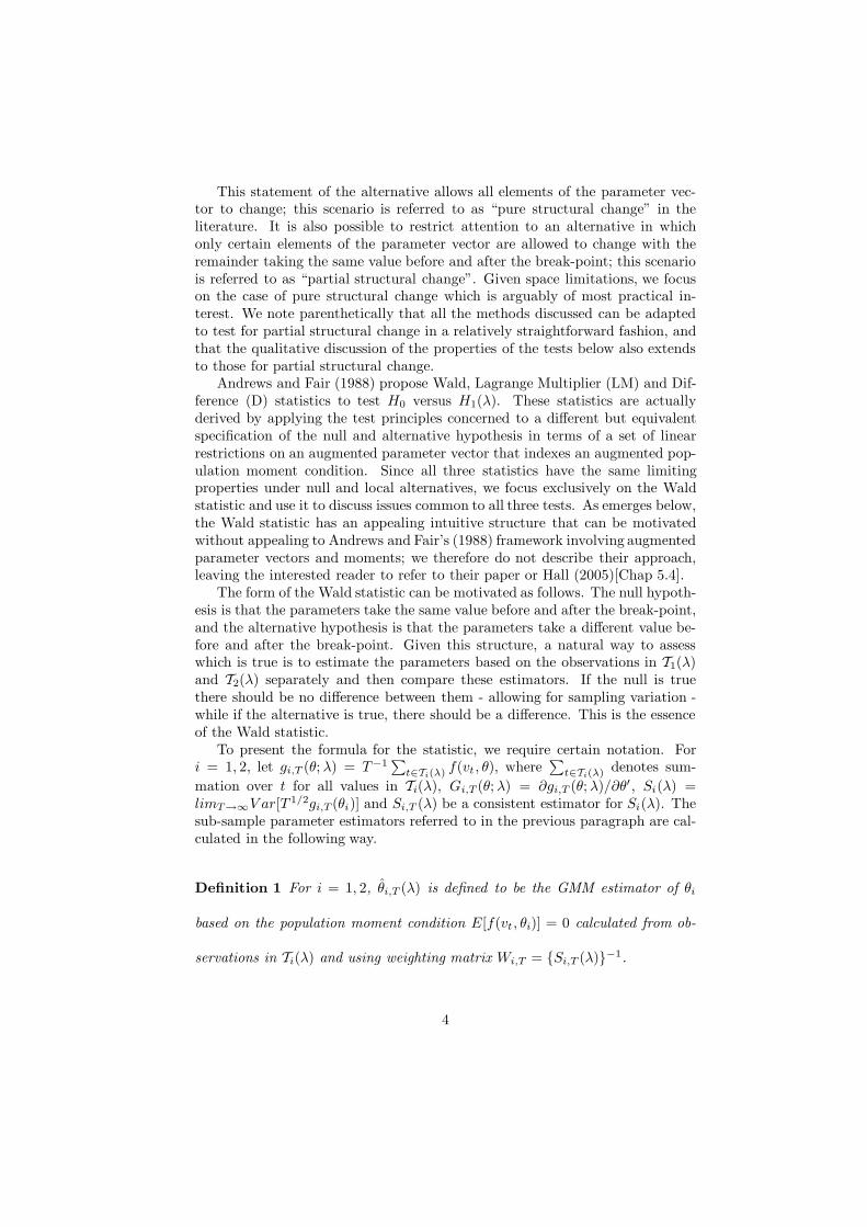
This statement of the alternative allows all elements of the parameter vec-tor to change; this scenario is referred to as “pure structural change” in theliterature. It is also possible to restrict attention to an alternative in whichonly certain elements of the parameter vector are allowed to change with theremainder taking the same value before and after the break-point; this scenariois referred to as “partial structural change”. Given space limitations, we focuson the case of pure structural change which is arguably of most practical in-terest. We note parenthetically that all the methods discussed can be adaptedto test for partial structural change in a relatively straightforward fashion, andthat the qualitative discussion of the properties of the tests below also extendsto those for partial structural change.

Andrews and Fair (1988) propose Wald, Lagrange Multiplier (LM) and Dif-ference (D) statistics to test H0 versus H1(λ). These statistics are actuallyderived by applying the test principles concerned to a different but equivalentspecification of the null and alternative hypothesis in terms of a set of linearrestrictions on an augmented parameter vector that indexes an augmented pop-ulation moment condition. Since all three statistics have the same limitingproperties under null and local alternatives, we focus exclusively on the Waldstatistic and use it to discuss issues common to all three tests. As emerges below,the Wald statistic has an appealing intuitive structure that can be motivatedwithout appealing to Andrews and Fair’s (1988) framework involving augmentedparameter vectors and moments; we therefore do not describe their approach,leaving the interested reader to refer to their paper or Hall (2005)[Chap 5.4].

The form of the Wald statistic can be motivated as follows. The null hypoth-esis is that the parameters take the same value before and after the break-point,and the alternative hypothesis is that the parameters take a different value be-fore and after the break-point. Given this structure, a natural way to assesswhich is true is to estimate the parameters based on the observations in T1(λ)and T2(λ) separately and then compare these estimators. If the null is truethere should be no difference between them - allowing for sampling variation -while if the alternative is true, there should be a difference. This is the essenceof the Wald statistic.

To present the formula for the statistic, we require certain notation. Fori = 1, 2, let gi,T (θ; λ) = T−1

∑t∈Ti(λ) f(vt, θ), where

∑t∈Ti(λ) denotes sum-

mation over t for all values in Ti(λ), Gi,T (θ; λ) = ∂gi,T (θ; λ)/∂θ′, Si(λ) =limT→∞V ar[T 1/2gi,T (θi)] and Si,T (λ) be a consistent estimator for Si(λ). Thesub-sample parameter estimators referred to in the previous paragraph are cal-culated in the following way.

Definition 1 For i = 1, 2, θi,T (λ) is defined to be the GMM estimator of θi

based on the population moment condition E[f(vt, θi)] = 0 calculated from ob-

servations in Ti(λ) and using weighting matrix Wi,T = {Si,T (λ)}−1.

4

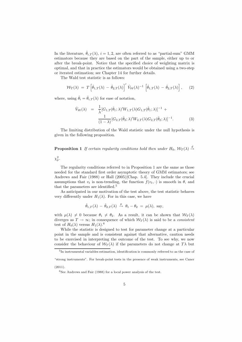
In the literature, θi,T (λ), i = 1, 2, are often referred to as “partial-sum” GMMestimators because they are based on the part of the sample, either up to orafter the break-point. Notice that the specified choice of weighting matrix isoptimal, and that in practice the estimators would be obtained using a two-stepor iterated estimation; see Chapter 14 for further details.

The Wald test statistic is as follows:

WT (λ) = T[θ1,T (λ) − θ2,T (λ)

]′VW (λ)−1

[θ1,T (λ) − θ2,T (λ)

], (2)

where, using θi = θi,T (λ) for ease of notation,

VW (λ) =1λ

[G1,T(θ1; λ)′W1,T (λ)G1,T (θ1; λ)]−1 +

1(1 − λ)

[G2,T (θ2; λ)′W2,T (λ)G2,T (θ2; λ)]−1. (3)

The limiting distribution of the Wald statistic under the null hypothesis isgiven in the following proposition.

Proposition 1 If certain regularity conditions hold then under H0, WT (λ) d→

χ2p.

The regularity conditions referred to in Proposition 1 are the same as thoseneeded for the standard first order asymptotic theory of GMM estimators; seeAndrews and Fair (1988) or Hall (2005)[Chap. 5.4]. They include the crucialassumptions that vt is non-trending, the function f(vt, ·) is smooth in θ, andthat the parameters are identified.5

As anticipated in our motivation of the test above, the test statistic behavesvery differently under H1(λ). For in this case, we have

θ1,T (λ) − θ2,T (λ)p→ θ1 − θ2 = µ(λ), say,

with µ(λ) 6= 0 because θ1 6= θ2. As a result, it can be shown that WT (λ)diverges as T → ∞; in consequence of which WT (λ) is said to be a consistenttest of H0(λ) versus H1(λ).6

While the statistic is designed to test for parameter change at a particularpoint in the sample and is consistent against that alternative, caution needsto be exercised in interpreting the outcome of the test. To see why, we nowconsider the behaviour of WT (λ) if the parameters do not change at Tλ but

5In instrumental variables estimation, identification is commonly referred to as the case of

“strong instruments”. For break-point tests in the presence of weak instruments, see Caner

(2011).6See Andrews and Fair (1988) for a local power analysis of the test.

5

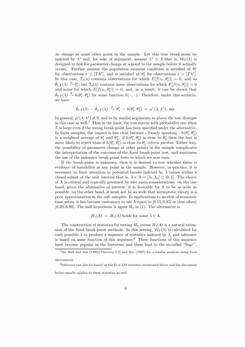
do change at some other point in the sample. Let this true break-point beindexed by λ∗ and, for sake of argument, assume λ∗ > λ that is, WT (λ) isdesigned to test for parameter change at a point in the sample before it actuallyoccurs. Further assume the population moment condition is satisfied at θ∗1for observations t ≤ [Tλ∗], and is satisfied at θ∗2 for observations t > [Tλ∗].In this case, T1(λ) contains observations for which E[f(vt, θ

∗1)] = 0, and so

θ1,T (λ) p→ θ∗1 ; but T2(λ) contains some observations for which E[f(vt, θ∗1)] = 0

and some for which E[f(vt, θ∗2)] = 0, and, as a result, it can be shown that

θ2,T (λ)p→ h(θ∗1 , θ∗2) for some function h( · , · ). Therefore, under this scenario,

we have

θ1,T (λ) − θ2,T (λ)p→ θ∗1 − h(θ∗1 , θ∗2) = µ∗(λ, λ∗), say.

In general, µ∗(λ, λ∗) 6= 0, and so by similar arguments to above the test divergesin this case as well.7 Thus in the limit, the test rejects with probability one whenT is large even if the wrong break-point has been specified under the alternative.In finite samples, the impact is less clear because - loosely speaking - h(θ∗1 , θ∗2)is a weighted average of θ∗1 and θ∗2 : if h(θ∗1 , θ∗2) is close to θ∗2 then the test ismore likely to reject than if h(θ∗1 , θ∗2) is close to θ∗1 ceteris paribus. Either way,the possibility of parameter change at other points in the sample complicatesthe interpretation of the outcome of the fixed break-point test, and motivatesthe use of the unknown break-point tests to which we now turn.

If the break-point is unknown, then it is desired to test whether there isevidence of instability at any point in the sample. However, in practice, it isnecessary to limit attention to potential breaks indexed by λ values within aclosed subset of the unit interval that is, λ ∈ Λ = [λl, λu] ⊂ [0, 1]. The choiceof Λ is critical and typically governed by two main considerations: on the onehand, given the alternative of interest, it is desirable for Λ to be as wide aspossible; on the other hand, it must not be so wide that asymptotic theory is apoor approximation in the sub–samples. In applications to models of economictime series, it has become customary to use Λ equal to [0.15, 0.85] or (less often)[0.20, 0.80]. The null hypothesis is again H0 in (1). The alternative is

H1(Λ) = H1(λ) holds for some λ ∈ Λ.

The construction of statistics for testing H0 versus H1(Λ) is a natural exten-sion of the fixed break-point methods. In this setting, WT (λ) is calculated foreach possible λ to produce a sequence of statistics indexed by λ, and inferenceis based on some function of this sequence.8 Three functions of this sequencehave become popular in the literature and these lead to the so-called “Sup-”,

7See Hall and Sen (1999)[Theorem 3.2] and Sen (1997) for a similar analysis using local

alternatives.8Inference can also be based on the D or LM statistics mentioned above and the discussion

below equally applies to these statistics as well.

6

“Av-” and “Exp-” statistics which are respectively given by,9

SupWT = supλ∈Λ

{WT (λ) },

AvWT =∫

Λ

WT (λ)dJ(λ),

ExpWT = log

{ ∫

Λ

exp[0.5WT (λ)]dJ(λ)}

,

where J(λ) = (λu − λl)−1dλ. As they stand these statistics are not operationalbecause we have treated λ as continuous, whereas in practice it is discrete.For a given sample size, the set of possible break-points are Tb = {i/T ; i =[λlT ], [λlT ] + 1, . . . , [λuT ]}. So in practice, inference is based on the discreteanalogs to SupWT , AvWT and ExpWT :

SupWT = supi∈Tb

{WT (i/T ) }

AvWT = d−1b

[λuT ]∑

i=[λlT ]

WT (i/T )

ExpWT = log

d−1

b

[λuT ]∑

i=[λlT ]

exp[0.5WT(i/T )]

where db = [λuT ] − [λlT ] + 1. Various statistical arguments can be made tojustify one statistic over another, but it has become common practice to reportall three in the empirical literature.

The limiting distribution of the three statistics is given in the followingproposition.10

Proposition 2 If certain regularity conditions hold then under H0, then we

have: SupWT ⇒ Supλ∈ΛW(λ), AvWT ⇒∫ΛW(λ)dJ(λ), and ExpWT ⇒

9This function is chosen to maximize power against a local alternative in which a weighting

distribution is used to indicate the relative importance of departures from parameter constancy

in different directions ( i.e. θ1−θ2) at different break-points and also the relative importance of

different break-points; see Andrews and Ploberger (1994) and Sowell (1996). The distribution

over break-points is commonly taken to be uniform on Λ which is imposed in the presented

formulae (via the specified J(π)) for the Av- and Exp- statistics in the text.10For regularity conditions and proofs see: Sup-test, Andrews (1993); Av-, Exp- tests,

Andrews and Ploberger (1994) (in context of maximum likelihood) and Sowell (1996) (in

context of GMM). In this context “⇒” denotes weak convergence in distribution.

7

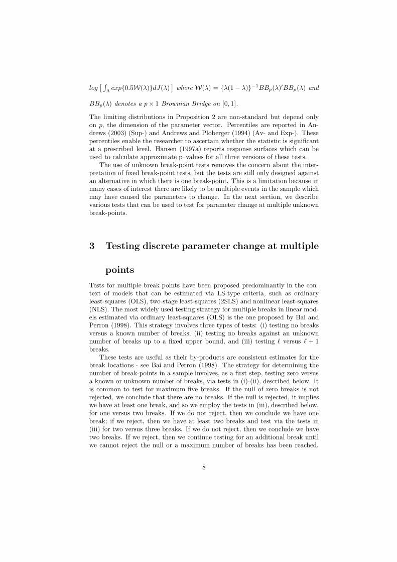
log[ ∫

Λ exp{0.5W(λ)}dJ(λ)]

where W(λ) = {λ(1 − λ)}−1BBp(λ)′BBp(λ) and

BBp(λ) denotes a p × 1 Brownian Bridge on [0, 1].

The limiting distributions in Proposition 2 are non-standard but depend onlyon p, the dimension of the parameter vector. Percentiles are reported in An-drews (2003) (Sup-) and Andrews and Ploberger (1994) (Av- and Exp-). Thesepercentiles enable the researcher to ascertain whether the statistic is significantat a prescribed level. Hansen (1997a) reports response surfaces which can beused to calculate approximate p–values for all three versions of these tests.

The use of unknown break-point tests removes the concern about the inter-pretation of fixed break-point tests, but the tests are still only designed againstan alternative in which there is one break-point. This is a limitation because inmany cases of interest there are likely to be multiple events in the sample whichmay have caused the parameters to change. In the next section, we describevarious tests that can be used to test for parameter change at multiple unknownbreak-points.

3 Testing discrete parameter change at multiple

points

Tests for multiple break-points have been proposed predominantly in the con-text of models that can be estimated via LS-type criteria, such as ordinaryleast-squares (OLS), two-stage least-squares (2SLS) and nonlinear least-squares(NLS). The most widely used testing strategy for multiple breaks in linear mod-els estimated via ordinary least-squares (OLS) is the one proposed by Bai andPerron (1998). This strategy involves three types of tests: (i) testing no breaksversus a known number of breaks; (ii) testing no breaks against an unknownnumber of breaks up to a fixed upper bound, and (iii) testing ` versus ` + 1breaks.

These tests are useful as their by-products are consistent estimates for thebreak locations - see Bai and Perron (1998). The strategy for determining thenumber of break-points in a sample involves, as a first step, testing zero versusa known or unknown number of breaks, via tests in (i)-(ii), described below. Itis common to test for maximum five breaks. If the null of zero breaks is notrejected, we conclude that there are no breaks. If the null is rejected, it implieswe have at least one break, and so we employ the tests in (iii), described below,for one versus two breaks. If we do not reject, then we conclude we have onebreak; if we reject, then we have at least two breaks and test via the tests in(iii) for two versus three breaks. If we do not reject, then we conclude we havetwo breaks. If we reject, then we continue testing for an additional break untilwe cannot reject the null or a maximum number of breaks has been reached.

8

This is a simple sequential strategy for estimating the number of breaks, andprovided the significance level of each test is shrunk in each step towards zero11,we will obtain the true number of breaks with probability one for large T .

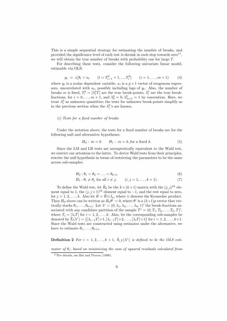
For describing these tests, consider the following univariate linear model,estimable via OLS:

yt = x′tθi + ut (t = T 0

i−1 + 1, ..., T 0i ) (i = 1, . . . , m + 1) (4)

where yt is a scalar dependent variable, xt is a p× 1 vector of exogenous regres-sors, uncorrelated with ut, possibly including lags of yt. Also, the number ofbreaks m is fixed, T 0

i = [λ0i T ] are the true break-points, λ0

i are the true break-fractions, for i = 0, . . . , m + 1, and λ0

0 = 0, λ0m+1 = 1 by convention. Here, we

treat λ0i as unknown quantities; the tests for unknown break-points simplify as

in the previous section when the λ0i ’s are known.

(i) Tests for a fixed number of breaks

Under the notation above, the tests for a fixed number of breaks are for thefollowing null and alternative hypotheses:

H0 : m = 0 H1 : m = k, for a fixed k. (5)

Since the LM and LR tests are asymptotically equivalent to the Wald test,we restrict our attention to the latter. To derive Wald tests from their principles,rewrite the null hypothesis in terms of restricting the parameters to be the sameacross sub-samples:

H0 : θ1 = θ2 = . . . = θk+1 (6)H1 : θi 6= θj for all i 6= j, (i, j = 1, . . . , k + 1). (7)

To define the Wald test, let Rk be the k× (k+1) matrix with the (j, j)th ele-ment equal to 1, the (j, j +1)th element equal to −1, and the rest equal to zero,for j = 1, 2, . . . , k. Also let R = R⊗Ip, where ⊗ denotes the Kronecker product.Then H0 above can be written as Rkθc = 0, where θc is a (k+1)p vector that ver-tically stacks θ1, . . . , θk+1. Let λc = (0, λ1, λ2, . . . , λk, 1)′ the break-fractions as-sociated with any candidate partition of the sample T c = (0, T1, T2, . . . , Tk, T )′,where Ti = [λiT ] for i = 1, 2, . . . , k. Also, let the corresponding sub-samples bedenoted by Ti(λc) = {[λi−1T ]+1, [λi−1T ]+2, . . . , [λiT ]+1} for i = 1, 2, . . . , k+1.Since the Wald tests are constructed using estimates under the alternative, wehave to estimate θ1, . . . , θk+1.

Definition 2 For i = 1, 2, . . . , k + 1, θi,T (λc) is defined to be the OLS esti-

mator of θi, based on minimizing the sum of squared residuals calculated from11For details, see Bai and Perron (1998).

9

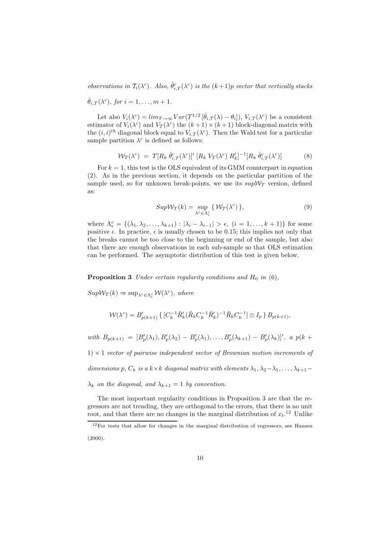
observations in Ti(λc). Also, θci,T (λc) is the (k+1)p vector that vertically stacks

θi,T (λc), for i = 1, . . . , m + 1.

Let also Vi(λc) = limT→∞V ar(T 1/2 [θi,T (λ) − θi]), Vi,T (λc) be a consistentestimator of Vi(λc) and VT (λc) the (k + 1)× (k + 1) block-diagonal matrix withthe (i, i)th diagonal block equal to Vi,T (λc). Then the Wald test for a particularsample partition λc is defined as follows:

WT (λc) = T [Rk θci,T (λc)]′ [Rk VT (λc) R′

k]−1[Rk θci,T (λc)] (8)

For k = 1, this test is the OLS equivalent of its GMM counterpart in equation(2). As in the previous section, it depends on the particular partition of thesample used, so for unknown break-points, we use its supWT version, definedas:

SupWT (k) = supλc∈Λc

ε

{WT (λc) }, (9)

where Λcε = {(λ1, λ2, . . . , λk+1) : |λi − λi−1| > ε, (i = 1, . . . , k + 1)} for some

positive ε. In practice, ε is usually chosen to be 0.15; this implies not only thatthe breaks cannot be too close to the beginning or end of the sample, but alsothat there are enough observations in each sub-sample so that OLS estimationcan be performed. The asymptotic distribution of this test is given below.

Proposition 3 Under certain regularity conditions and H0 in (6),

SupWT (k) ⇒ supλc∈ΛcεW(λc), where

W(λc) = B′p(k+1) { [C−1

k R′k(RkC−1

k R′k)−1RkC−1

k ] ⊗ Ip }Bp(k+1),

with Bp(k+1) = [B′p(λ1), B′

p(λ2) − B′p(λ1), . . . , B′

p(λk+1) − B′p(λk)]′, a p(k +

1) × 1 vector of pairwise independent vector of Brownian motion increments of

dimensions p, Ck is a k×k diagonal matrix with elements λ1, λ2−λ1, . . . , λk+1−

λk on the diagonal, and λk+1 = 1 by convention.

The most important regularity conditions in Proposition 3 are that the re-gressors are not trending, they are orthogonal to the errors, that there is no unitroot, and that there are no changes in the marginal distribution of xt.12 Unlike

12For tests that allow for changes in the marginal distribution of regressors, see Hansen

(2000).

10

for LR-type tests, these regularity conditions allow for heteroskedasticity andautocorrelation. In particular, they allow for the variance of ut to change at thesame time as the parameters. As pointed out by Lubik and Surico (2010), thisis an important feature of the SupWT (k) test that allows practitioners to testmore accurately for monetary policy breaks during the Great Moderation.

The SupWT (k) test is consistent against H1. For k = 1, its distributionreduces to the one in Proposition 1, and its optimality properties are the sameas for GMM settings13, but they are not known for k > 1. However, for mostpractical purposes, it suffices to know that in the OLS setting, the supWT (k)delivers consistent estimators of the true k break-fractions indexing the break-points.

(ii) Tests for an unknown number of breaks

The test in (9) also rejects with probability one when T is large, if thetrue number of breaks under the alternative is k∗ 6= k. However, if the truealternative is H1 : m = k∗, in small samples it might not have good powerproperties because it is not designed for this alternative. To address this issue,Bai and Perron (1998) propose a second set of tests, presented in (ii) below,against the alternative of an unknown number of breaks up to a maximum:

H0 : m = 0 H1 : 1 ≤ m ≤ M, for a fixed M. (10)

These tests are known as double-maximum or Dmax-type tests. The ideabehind these tests is to construct for each m ∈ {1, . . . , M} a supWT (m)-test(thus a maximum for each m), and then to maximize over weighted versionsof these statistics to obtain a unique test statistic for the null and alternativehypotheses in (5). This test is defined below:

DmaxWT = max1≤m≤M

am

pSupWT (m), (11)

for some fixed, strictly positive weights am. The distribution of this test gener-alizes in a straightforward fashion from Proposition 3:

Proposition 4 Under certain regularity conditions and H0,

DmaxWT ⇒ max1≤m≤M

am

psup

λc∈Λcε

m+1∑

i=1

Wi(λc)

13Corresponding AveWT and ExpWT and their optimality properties for one break in an

OLS setting are discussed in Kim and Perron (2009).

11

The regularity conditions are the same as for SupWT (m) test, for each m.The weights for the DmaxWT test should be set larger for a certain m if onebelieves that m is more likely to be the correct number of breaks. If there is noclear a-priori belief about the true number of breaks, one can use equal weightsam = 1/M , in which case the test is known as a UDmax test. However, notethat the scaling p is used because in its absence and with equal weights am, thistest will be equivalent to testing zero against M breaks, since the critical valuesincrease in m for a fixed p. Since, despite the scaling, the critical values stilltend to increase with m, let c(m, p, α) be the asymptotic critical value of thetest SupWT (m)/p at significance level 100α%.14 Then the problem of increasingcritical values is alleviated by setting a1 = 1 and am = c(1, p, α)/c(m, p, α), andthe corresponding test is called a WDmax test.

(iii) Tests for an additional break

The third category of tests for multiple breaks (iii) are called sequential Waldtests, since they are Wald tests for an additional break. The null and alternativehypotheses are, for any given `:

H0 : m = ` H1 : m = ` + 1. (12)

A LR-type test for is proposed in Bai and Perron (1998). However, asymp-totically equivalent Wald-type tests can be derived as a special case of thesequential Wald tests in Boldea and Hall (2010) and Hall, Han, and Boldea(2012). For the Wald test, one ideally uses the estimates only under the alter-native hypothesis.15 However, for computational ease, it has become routineamong practitioners to use Bai and Perron’s (1998) approach of pre-estimatingthe model with ` breaks. This implies that estimates of the ` breaks are ob-tained as a by-product of calculating the Wald statistic SupWT (`), imposed asif they were the true ones, and for the alternative hypothesis in (3), evidenceis maximized for exactly one additional break, occurring in only one of the` + 1 sub-samples obtained by partitioning the sample with the pre-estimated `breaks. To define the test, let µ denote each candidate additional break fractionin the pre-estimated ` + 1 sub-samples Λq(q = 1, 2, . . . , ` + 1), with

Λq = {µ : Tq−1 + (Tq − Tq−1)η ≤ [µT ] ≤ Tq − (Tq − Tq−1)η}.

In these sub-samples, the OLS parameter estimates before and after each can-didate additional break are denoted by ϑq(µ) = [θ1(µ, q)′, θ2(µ, q)′]′, whereq = 1, 2, . . ., `+1, and the restriction that they are equal is defined through therestriction matrix R∗ = [Ip;−Ip]. Then the sequential Wald test is:

14These critical values can be found in Bai and Perron (1998).15For an equivalent LR test that estimates the model in 4 with `, respectively ` + 1 breaks,

see Bai (2009).

12

WT (` + 1|`) = max1≤q≤`+1

supµ∈Λq

WT,`(µ, q) (13)

where

WT,`(µ, q) = T [R∗ϑq(µ)]′ [R∗V ∗T (µ, q)R∗′

]−1 R∗ϑq(µ)

and V ∗T (µ, q) is the 2p×2p block-diagonal matrix with diagonal blocks V1,T (µ, q)

and V2,T (µ, q). The latter two are defined as consistent estimators of theirasymptotic equivalents V1(µ, q) = limT→∞V ar T 1/2 [θ1(µ, q)− θq ], respectivelyV2(µ, q) = limT→∞V ar T 1/2 [θ2(µ, q) − θq], for q = 1, 2, . . . , ` + 1.

The asymptotic distribution of the test is described below:

Proposition 5 Under certain regularity conditions and H0 in (3), limP (WT (`+

1|`) ≤ x) = G`+1p,η , where Gp,η is the cumulative distribution function of

supη≤µ≤1−η

‖Bp(µ) − µBp(1)‖2

µ(1 − µ).

The regularity conditions follow directly from Hall, Han, and Boldea (2012),by treating all endogenous variables as exogenous. They allow for breaks inthe error variance occurring at the same time as the parameters under H1 in(3). Critical values for the tests (i)-(iii) can be found in Bai and Perron (1998),and p-values based on approximate response surfaces can be found in Hall andSakkas (2011).

As mentioned above, these tests are useful for models that can be estimatedby OLS, thus with exogenous regresssors. When some regressors are endoge-nous, Hall, Han, and Boldea (2012) show that a similar sequential procedurefor finding the number of breaks in models with endogenous regressors can bedeveloped, based on tests constructed with 2SLS estimates.

However, unlike for OLS, with 2SLS, one needs to first assess whether thereare any breaks in the first-stage regression. To see why this is important, assumethat the researcher has in mind an economic model, from which the first andsecond stages of 2SLS estimation arise naturally. For example, consider thefollowing structural model:

yt = θxt + ut (14)xt = γ1yt + γ2ht + γ3z1,t + v1,t (15)ht = δ1xt + δ2z2,t + v2,t (16)

where yt, xt, ht are scalar dependent variables, zt = (z1,t, z2,t)′ are scalar exoge-nous regressors, ut, v1,t, v1,t are errors and θ, γ1, γ2, γ3, δ1, δ2 are scalar unknownparameters that may break at unknown locations in the sample.

13

If one is interested in estimating θ, the equation of interest is (14), and willbe the second stage in a 2SLS regression, with the first stage instrumenting forthe endogeneity of xt via instruments zt. In this example, the first-stage arisesnaturally, since the reduced form for xt can be found by substituting (14) and(16) into (15):

xt = z′t∆ + vt (17)

∆ =(

γ3

1 − θγ1 − δ1γ2,

γ2δ2

1 − θγ1 − δ1γ2

)′

vt =γ1ut + v1,t + γ2v2,t

1 − θγ1 − δ1γ2.

In this context, we can see that all breaks in θ, thus in (14), will also be in(17) by default, unless γ1 = 0. When γ1 = 0, if no other parameters changebesides θ, (17) will have no breaks. If any of the parameters γj(j = 1, 2, 3), δ1, δ2

change, then these changes are only reflected in (17). Thus the first-stage canhave no breaks, or breaks that are common to the second-stage, or breaks thatare idiosyncratic to the first-stage.

In practice, one does not necessarily know which scenario occurs, so it isimportant to consider both the case where the first-stage is stable and where itis unstable. For simplicity, consider a data generating process with m and m∗

breaks in the second-, respectively first-stage regressions:

yt = xtθi + ut (t = T 0i−1 + 1, ..., T 0

i ) (i = 1, . . . , m + 1) (18)

where xt is a scalar endogenous regressor, i.e. correlated with ut, and thus needsto be predicted via the first stage OLS regression with s× 1 strong instrumentszt:

xt = z′t∆i + vt (t = T ∗j−1 + 1, ..., T ∗

j ) (j = 1, . . . , m∗ + 1) (19)

with ut correlated with vt, T0 = T ∗0 = 1, T 0

i = [λ0i T ], T ∗

j = [λ∗jT ], Tm+1 =

Tm∗+1 = T , and some breaks may be common to both equations.If there are no breaks in the first-stage, i.e. m∗ = 0, the 2SLS structural

stability tests are computed exactly as their OLS conterparts in (i)-(iii), butfor the second-stage equation (18), and with xt replaced by xt, its predictedcounterpart from an OLS regression in (17). For clarity, the 2SLS estimatorsare defined below.

Definition 3 For i = 1, 2, . . ., k+1, θi,T (λc) is defined to be the 2SLS estimator

of θi, based on minimizing the OLS sum of squared residuals calculated for

the second-stage (18), from observations in Ti(λc) - defined as before- using as

14

regressors xt instead of xt, where xt is the full-sample OLS estimator from the

first stage equation (17). Also, θcT (λc) is the (k+1)p vector that vertically stacks

θi,T (λc), for i = 1, . . . , m + 1.

(iv) Sequential testing strategy for stable first-stage regression

For sequential testing, the tests in (i)-(iii), SupWT , DmaxWT and WT (` +1|`), are defined in the same way as before, except that the 2SLS estimatorsreplace their OLS counterparts in the definition of the tests. As Hall, Han,and Boldea (2012) show, the asymptotic distributions of these tests are also thesame as in Propositions 3-5. Thus, a 2SLS sequential strategy for estimatingthe number and location of breaks can be constructed in the same way fromthese tests as before, when the first-stage equation (19) is stable.

However, in general (19) may also have breaks, i.e. m∗ 6= 0. One can testthis equation for breaks, and find their locations, via the OLS sequential testingstrategy in (i)-(iii). As discussed above, these tests also provide consistentestimators of the number of break-points, m∗ and their locations, T ∗

j , (j =1, 2, . . . , m∗).

It remains to find the number of breaks in the second-stage, for which xt, aprediction of xt based on estimating the first-stage equation (19), needs to becomputed. If one ignores the breaks found in (19) in computing xt, the 2SLStests in the second stage will pick up these breaks and reject with probabilityone for large T even if there are no breaks in the second-stage. If one computesxt by OLS in each sub-sample constructed via the estimates of T ∗

j , and thenproceeds with testing for breaks in the full-sample of the second stage (18) viathe tests in (i)-(iii), but with xt replaced by xt, then the asymptotic distributionsin Propositions 3-5 are no longer valid.16

Fortunately, there is a simple way to side-step these issues and sequentiallytest for breaks in (18). A strategy for finding these breaks is described below.

(v) Sequential testing strategy for unstable first-stage regression

(v-i) Tests for breaks that are idiosyncratic to the second-stage

If breaks are found in the first stage, a strategy for finding the breaks thatonly occur in the second stage is described below.

• Obtain estimates m∗ for the number of breaks m∗ and T ∗j (j = 1, . . . , m∗)

for the associated break-points T ∗j (j = 1, . . . , m∗), either as a by-product

of the OLS sequential strategy in (19), or by global estimation via the16These distributions are much more complicated and depend on the relative positioning of

the breaks in the first- and second-stage. To obtain critical values, bootstrap-based methods

are proposed - see Boldea, Cornea, and Hall (2011).

15

methods in Hall, Han, and Boldea (2012). If the sequential strategy isused, reduce in each step the critical value to make sure that m∗ = m∗

with probability one as T grows larger. This ensures that we can treat m∗

as if it were m∗ in the next steps.

• Split the sample into sub-samples T ∗j = {T ∗

j−1 + 1, T ∗j−1 + 2, . . . , T ∗

j } for(j = 1, . . . , m∗). In each sub-sample T ∗

j , compute xt via OLS, and runthe sequential testing strategy in (iv) for each of these sub-samples of thesecond-stage model (18).

• As a by-product of the testing strategy, or the re-estimation of the breaksin sub-samples T ∗

j - see Boldea, Hall, and Han (2012) - one obtains con-sistent estimates of the non-common break fractions in (18). Denote theirbreak-point counterparts by Tn, (n = 1, 2, . . ., N ), with N ≤ m. Theseare the breaks that are idiosyncratic to the second-stage.

• Let T0 = 0 and TN+1 = T , to include sample ends. Obtain the unionof sample end-points and the breaks in the first-stage and second-stage,ordered, as B = {T0, . . . , TN+1}∪ {T ∗

1 , . . . , T ∗m∗}. Thus, B contains all the

breaks in the first- and second-stage equation (18) and (19).

Thus, via this strategy, the researcher knows the idiosyncratic breaks to thesecond-stage, and all the breaks in the first-stage. However, for practical pur-poses, one needs to know which breaks are common to the two stages. Thisis not only important for correct estimation of the sub-samples in the second-stage, it is also of interest to practitioners. For example, in the estimation of ahybrid NKPC, with measured expectations, Boldea, Hall, and Han (2012) showthat a break at the end of 1980 occurred in the modeled inflation expectations,but that break did not further occur in the NKPC itself once the change in ex-pectations was taken into account. The test they use to detect common breaksis a usual Wald test for a known break-point, and is defined below.

(v-ii) Tests for breaks that are common to both stages

To describe these tests, let the ordered breaks in B be T1, T2, . . . , TH , withH = m∗ + N . Then for any s = 1, 2, . . . , H such that T ∗

j = Ts, take thesmallest sub-sample encompassing it, {Ts−1 + 1, . . . , Ts+1}, and calculate the2SLS estimators θs and θs+1, based on sub-samples Bs = {Ts−1 + 1, . . . , Ts},respectively Bs+1 = {Ts + 1, . . . , Ts+1}. Treat the end-points Ts−1 and Ts+1,and T ∗

j as known. Then the Wald test for a common break Ts, to both equations(18) and (19), is:

WT = T (θs − θs+1)′[Vs,T + Vs+1,T ]−1(θs − θs+1), (20)

where Vi,T are consistent estimates of the asymptotic variances Vi = limT→∞V ar

[T 1/2(θi − θi)], for i = s, s + 1. Because we test in the second-stage for a break

16

pre-estimated from another equation, the first-stage, the distribution is the sameas if the break-point Ts were known.

Proposition 6 Under certain regularity conditions17, under the null hypothesis

of no common break in the sub-sample tested,

WTd→ χ2

1 (21)

Thus, all the breaks in the equation of interest (18) can be retrieved viathe sequential strategy in (v) - or (iv) if no breaks are found in the first-stageregression.

This procedure was defined for one endogenous regressor, but can be gen-eralized to p multiple endogenous regressors Xt. Intuitively, one just needs toconsistently predict the endogenous regressors from the first stage, so the OLSsequential strategy in (i)-(iii) can be applied to the first stage equation pertain-ing to each endogenous regressor separately.18 If the second-stage equation alsohas exogenous regressors at, then the tests in (iv)-(v) remain valid, with xt re-placed by (X ′

t, a′t)′. The optimality of these procedures is, as for OLS methods,

unclear, but all the tests reject with probability one for large T , regardless ofwhether the breaks are small or large.

In nonlinear models, a similar sequential procedure as in (i)-(iii) is availablefor models that can be estimated via nonlinear least squares - see Boldea andHall (2010). Given a known parametric regression function with multiple pa-rameter changes, the tests in (i)-(iii) remain valid, and so do their distributions,as long as the OLS estimators in (i)-(iii) are replaced by their NLS counterparts.

Even though a procedure for testing for multiple breaks in linear modelsestimated via GMM is not known, its 2SLS counterpart can be used, and as abyproduct, one obtains consistent break-points as well as parameter estimates.Thanks to the dynamic programming algorithm introduced in Bai and Perron(2003), the computational burden for a sample size of T is less than T (T + 1)/2operations independent of the number of breaks. GAUSS code for testing formultiple breaks can be found at http : //people.bu.edu/perron/code.html forOLS methods.

The testing procedures above are all designed for multiple breaks, whenthe parameter changes infrequently and permanently from one value to anotherat a few locations in the sample. Other types of parameter instability aresummarized in the next section.

17See Hall, Han, and Boldea (2012).18For estimating the breaks by considering a multivariate first-stage for all endogenous

regressors jointly, a comprehensive procedure can be found in Qu and Perron (2007).

17

4 Testing for other types of parameter change

Break-points are by default exogenous to the model, since time is an exoge-nous quantity. When parameter changes are believed to be driven by someobserved variables that indicate the state of the business cycle or some otherimportant economic indicators, researchers resort to other types of parameterchange models, called threshold and smooth transition models.

Threshold and smooth transition models have been used to model GDPgrowth, unemployment, interest rates, prices, stock returns and exchange rates- for a review of the empirical and theoretical econometrics literature, see vanDijk, Terasvirta, and Franses (2002) and Hansen (2011).

The threshold model, introduced by Howell Tong19, resembles in many waysthe break-point model. To see the connection, for simplicity we revert to anexposition with one break. Thus, consider the model (4) but m = 1, re-writtenin the following way:

yt = x′tθt + ut with θt = θ1 + (θ2 − θ1)1{t ≥ T1} (22)

where 1 is the indicator function. If instead, θt is defined as:

yt = x′tθt + ut with θt = θ1 + (θ2 − θ1)1{qt ≥ c}, (23)

where yt is a scalar dependent variables, c is an unknown parameter, to beestimated, and xt and qt are exogenous observed regressors, uncorrelated withut, one obtains the threshold model. If xt contains lags of yt, this model is knownas the threshold autoregressive (TAR) model.

In this model, the parameter change is driven by the observed variable qt,called a state variable, and c denotes the threshold above which the parametersof the model change from θ1 to θ2. If one orders the data (yt, xt) on the valuesof qt, say in ascending order, one obtains two sub-samples, one for which thetrue parameter is θ1, and another for which the true parameter is θ2. Thesetwo sub-samples resemble the break-point sub-samples; the break-point here isthe point in the newly ordered sample where qt changes from a value below cto a value above c. Hansen (1997b) shows that by re-ordering of the data asdescribed above, a supWT of the type described in the previous section can beconstructed, and its asymptotic distribution for one threshold is the same asin Proposition 3 for k = 1. This procedure is extended to estimating multiplethresholds in Gonzalo and Pitarakis (2002).

When some of the regressors in xt are endogenous, but qt is exogenous, forone threshold model, Caner and Hansen (2004) propose the sup-type Wald testconstructed with a 2SLS estimator of the threshold c and GMM estimators ofthe other parameters. Its asymptotic distribution is computed by simulationin Caner and Hansen (2004). For endogenous qt, no tests are known so far,although estimation of models with one endogenous threshold can be done via2SLS estimation with bias correction - see Kourtellos, Stengos, and Tan (2008).

19For an early review of the threshold literature in statistics, see Tong (1983).

18

An equally influential model in empirical macroeconomics is the smoothtransition autoregressive (STAR) model, introduced by Terasvirta (1994). Thismodel is mostly suitable for policy functions such as the interest rate functions,where the parameter is not changing in a sudden fashion from θ1 to θ2, but ina smooth way. The smoothness is imputed by replacing the indicator functionwith a smooth function, with values in the interval (0, 1), meaning that trueparameters at each point in time no longer take two values, θ1 and θ2, but aremost of the time in-between these values. We present here the simplest STARmodel, called the logistic STAR, where the indicator function is replaced by thesmooth logistic function f(·, ·, ·), defined below:

yt = x′tθt + ut with θt = θ1 + (θ2 − θ1)f(qt, γ, c) (24)

f(qt, γ, c) =exp{γ(qt − c)}

1 + exp{γ(qt − c)} (25)

Here qt and xt are observed and uncorrelated with the errors ut, and maycontain lags of yt, γ is an unknown smoothness parameter and c is the unknown’threshold’ parameter. The latter two need to be estimated. When γ is large,the transition is faster as the transition function moves faster from 0 to 1 whenqt is above c; when γ is small, the transition is slower.

This model is different than the threshold or break model in the sense thatit can be written as a smooth nonlinear regression. Unfortunately, the usualnonlinear regression Wald tests do not directly apply. The reason is because,under the null hypothesis of θ1 = θ2, or no nonlinearity, the parameters γ, care not identified, since any value of these parameters will render the samelinear regression function. This implies that we may have a similar problem tothe break-point or threshold model, of unidentified parameters under the nullhypothesis. However, because the regression function in (23) is smooth underthe alternative, one can write a third-order Taylor expansion of f(qt, ·, c) aroundγ = 0. This yields a model that has the parameters γ, c also identified underthe null hypothesis, and Eitrheim and Terasvirta (1996) show that the resultingmodel can be tested for no nonlinearity via a usual LM test. If one doesn’t usethis expansion, the optimality properties of a Sup-type LR test over all possiblevalues of γ, c, are studied in Andrews, Cheng, and Guggenberger (2011), whoshow that this test may not have the right size.

STAR models have recently been shown to be estimable via GMM in thepresence of endogenous regressors using the usual GMM asymptotic theory -see Areosa, McAleer, and Medeiros (2011). Thus, we conjecture that the testsdiscussed here for STAR models can be used in their equivalent GMM formwith no further complications.

So far, we have discussed models for parameter change driven by an observedvariable. However, one may think that the behavior of macroeconomic variableschanges with an unobserved variable such as the state of the business cycle. Suchmodels are called regime-switching models (or Markov-switching under certainregularity conditions) and were introduced in econometrics by Hamilton (1989).To write down a Markov-switching model, let st be an unobserved state variable,

19

with values zero or one (i.e. for recession or expansion). Then:

yt = x′tθt + ut with θt = θ1 + (θ2 − θ1)st (26)

P (st = 1|st−1 = 1, It) = p1; P (st = 0|st−1 = 0, It) = p2 (27)

Here, xt usually includes some lags of yt, and is uncorrelated with ut. Also, st ∈{0, 1}, and the probabilities of being in a certain state are entirely determinedby the previous state and the information set at time t, It, which includes xt

and all its previous values.Suppose one wants to test whether the parameter change θ2 − θ1 is zero or

not. In this case, p and q are the parameters that not identified under the nullhypothesis, but there are other complications related to the cases of p or q beingclose to zero or one. This presence implies that we cannot use Taylor expansionsas in the STAR example to test for parameter change. Hansen (1992) proposesan upper bound for a sup-type LR test, but this bound depends on the dataand is often burdensome to compute. Garcia (1998) proposes to restrict testingto cases where p, q are bounded away from 0, 1, and use the sup-LR test, wherethe supremum is taken over (p, q), and gives the asymptotic distribution of thetest. However, because the framework he uses to justify his test, taken fromAndrews and Ploberger (1994), does not apply to Markov-switching models,this test may not have optimal power. To that end, we recommend the test byCarrasco, Hu, and Ploberger (2009), an information-matrix type LM test thatis shown to have certain desired optimality properties.

When xt is endogenous, Kim (2004) and Kim (2009) show that either a bias-corrected maximum-likelihood estimation or a two-step maximum likelihoodignoring the bias can be used the estimate the Markov-switching model withtwo regimes. Similarly, when st is endogenous but xt are exogenous, Kim, Piger,and Startz (2008) propose a bias-corrected filter to estimate the model. As forSTAR, we conjecture that tests can be constructed based on these inferenceprocedures, adapted from the Markov switching tests for exogenous regressors.

There are many other types of parameter change, but the main types aresummarized here and they all have their merits for the applied researcher.

5 Testing for other types of structural instabil-

ity

So far, the focus of this chapter has been on testing for parameter change;however this is not the only scenario that can lead to structural instability. Inthis section, we explore tests for other forms of structural instability that havebeen developed within the GMM framework. To this end, we return to theframework in Section 2.

20

A natural alternative to H0 in (1) that captures the notion of structuralinstability at a fixed break-point T1 = [Tλ] is

H ′1(λ) : E[f(vt, θ0)] = 0, for t = 1, 2, . . . , T1,

E[f(vt, θ0)] 6= 0, for t = T1 + 1, . . . , T.

Under H ′1(λ), the population moment holds at θ0 before the break-point, but

fails to hold after. Before proceeding further, we note that all that followsapplies equally if the population moment condition holds at θ0 after but notbefore the break-point.

If q = p - and so there are the same number of moment conditions as param-eters - then it can be shown that H1(λ) and H ′

1(λ) are equivalent.20 However,if q > p - and so there are more moment conditions than parameters - then thisequivalence does not hold. Exploiting the decomposition of the population mo-ment condition inherent in GMM estimation,21 Hall and Sen (1999) show thatH ′

1(λ) can be decomposed into two parts: structural instability in the identifyingrestrictions at [Tλ] and structural instability in the overidentifying restrictionsat [Tλ]. Instability of the identifying restrictions is equivalent to H1(λ) that is,to parameter change at Tλ. Instability of the overidentifying restrictions meansthat some aspect of the model beyond the parameters alone has changed at [Tλ].Rather than specifying this alternative mathematically, we present an intuitiveexplanation. To this end, consider Hansen and Singleton’s (1982) consumptionbased asset pricing in which a representative agent makes consumption and in-vestment decisions to to maximize discounted expected lifetime utility based ona utility function,

Ut(ct) =cγt − 1

γ.

The parameters of this model are γ, with 1 − γ being the coefficient of relativerisk aversion, and β, the discount factor; so, in our notation, θ = (γ, β)′. It iscustomary to estimate θ0 via GMM based on E[ut(θ0)zt] = 0 where ut(θ0) isthe so-called Euler residual derived from the underlying economic model, and zt

is a vector of variables contained in the representative agent’s information set.Within this setting, H1(λ) implies that the parameters have changed but thefunctional form of ut(θ) has stayed the same: this state of the world occurs ifthe functional form of the agent’s utility function is the same before and afterthe break-point but either his/her coefficient of relative risk aversion or his/herdiscount factor changes. Instability of the overidentifying restrictions impliesthat the structural change involves more than the parameters: this state of theworld would occur if the functional form of the agent’s utility function changesat the break-point.

Since instability of the identifying and overidentifying restrictions have dif-ferent implications for the underlying model, Hall and Sen (1999) argue that it

20This result presumes certain (relatively weak) regularity conditions hold and can be es-

tablished via a similar argument to Hall and Inoue (2003)[Proposition 1].21For example, see Chapter 14.

21

is advantageous to test H0(λ) against each separately. To test against instabil-ity of the identifying restrictions, we can use the statistics for testing againstH1(λ) described in Section 2. To test against instability of the overidentifyingrestrictions, Hall and Sen (1999) propose the use of the following statistic,

OT (λ) = O1,T (λ) + O2,T (λ)

where Oi,T (λ) is the overidentifying restrictions tests based on the sub–sampleTi for i = 1, 2.22 The following proposition gives the limiting distribution ofOT (λ).

Proposition 7 If certain regularity conditions hold then under H0, then we

have: OT (λ) d→ χ2(q−p).

Hall and Sen (1999) show that under H0, OT (λ) is asymptotically independentof the statistics, such as WT (λ), used to test parameter change. They furthershow that under local alternatives each of WT (λ) and OT (λ) has power againstits own specific alternative but none against the alternative of the other test.These properties underscore the notion that the two statistics are testing differ-ent aspects of instability and provides some guidance on the interpretation ofsignificant statistics, although the local nature of the results needs to be keptin mind.23

Hall and Sen (1999) also propose the following statistics for testing for in-stability of the overidentifying restrictions at an unknown break-point,24

SupOT = supi∈Tb

{OT (i/T ) }

AvOT = d−1b

[λuT ]∑

i=[λlT ]

OT (i/T )

ExpOT = log

d−1

b

[λuT ]∑

i=[λlT ]

exp[0.5OT (i/T )]

The limiting distribution of these statistics is as follows.22See Chapter 14 for a description of the overidentifying restrictions test.23To elaborate, WT (λ) significant but OT (λ) insignificant is consistent with instability

confined to the parameters alone; OT (λ) significant is consistent with more general forms of

instability. However, important caveats are the local nature of these results and concerns

about the interpretation of fixed break-point tests discussed in Section 2.24Although the functionals are the same as the parameter change tests, it has proved im-

possible to date to deduce any optimality properties for the versions based on OT (λ) due to

the nature of the alternative in this case; see Hall (2005)[p.182] for further discussion.

22

Proposition 8 If certain regularity conditions hold then under H0, then we

have: SupOT ⇒ Supλ∈ΛO(λ), AvOT ⇒∫ΛO(λ)dJ(λ), and

ExpOT ⇒ log[ ∫

Λexp{0.5O(λ)}dJ(λ)

]where O(λ) = 1

λB′q−pBq−p+ 1

1−λ [Bq−p(1)−

Bq−p(λ)]′[Bq−p(1)−Bq−p(λ)] and Bq−p(λ) denotes a (q− p)× 1 Brownian mo-

tion on [0, 1].

The limiting distributions in Proposition 8 are non-standard but depend onlyon q − p, the number of overidentifying restrictions. The percentiles of theselimiting distributions are reported in Hall and Sen (1999). Sen and Hall (1999)report response surfaces which can be used to calculate approximate p–valuesfor all three versions of these tests.

6 Conclusions

In this chapter, we describe various structural stability tests that are best suitedfor empirical analysis in macroeconomics. We discuss tests for parameter breaks,other types or parameter changes and also model instability. Most of our dis-cussion is focused around Wald-type tests, that are robust to heteroskedasticityand autocorrelation. The tests we described do not cover all possible scenarios,such as the presence of unit roots, long memory, cointegrating relationships.Instead, we strive to provide practitioners with a broad set of tools that covermost cases of interest - excluding the above - in empirical macroeconometrics.We emphasize on structural stability tests for models with exogenous and en-dogenous regressors and the differences between the two.

The tools we summarize here can be readily applied to a wide range ofmacroeconomic and monetary policy models, contributing to important macroe-conomic debates such as whether the New Keynesian Phillips curve has becomeless predictable, or whether the Great Moderation is due to good monetarypolicy or good luck - see Lubik and Surico (2010).

23

References

Alogoskoufis, G., and Smith, R. (1991). ‘The Phillips curve, the persistenceof inflation, and the Lucas critique: Evidence from exchange-rate regimes’,American Economic Review, pp. 1254–1275.

Andrews, D., Cheng, X., and Guggenberger, P. (2011). ‘Generic results for estab-lishing the asymptotic size of confidence sets and tests’, Cowles FoundationDiscussion Paper No. 1813.

Andrews, D. W. K. (1993). ‘Tests for parameter instability and structural changewith unknown change point’, Econometrica, 61: 821–856.

(2003). ‘Tests for parameter instability and structural change with un-known change point: a corrigendum’, Econometrica, 71: 395–398.

Andrews, D. W. K., and Fair, R. (1988). ‘Inference in econometric models withstructural change’, Review of Economic Studies, 55: 615–640.

Andrews, D. W. K., and Ploberger, W. (1994). ‘Optimal tests when a nuisanceparameter is present only under the alternative’, Econometrica, 62: 1383–1414.

Areosa, W., McAleer, M., and Medeiros, M. (2011). ‘Moment-based estimationof smooth transition regression models with endogenous variables’, Journalof Econometrics, 165: 100–111.

Bai, J. (2009). ‘Likelihood ratio tests for multiple structural changes’, Journalof Econometrics, 91: 299–323.

Bai, J., and Perron, P. (1998). ‘Estimating and testing linear models with mul-tiple structural changes’, Econometrica, 66: 47–78.

(2003). ‘Computation and Analysis of Multiple Structural Change Mod-els’, Journal of Applied Econometrics, 18: 1–23.

Ben-David, D., Lumsdaine, R., and Papell, D. (2003). ‘Unit roots, postwar slow-downs and long-run growth: Evidence from two structural breaks’, EmpiricalEconomics, 28(2): 303–319.

Benati, L., and Surico, P. (2008). ‘Evolving US monetary policy and the declineof inflation predictability’, Journal of the European Economic Association,6(2-3): 634–646.

Boivin, J., and Giannoni, M. (2006). ‘Has monetary policy become more effec-tive?’, The Review of Economics and Statistics, 88(3): 445–462.

Boldea, O., Cornea, A., and Hall, A. (2011). ‘Bootstrapping multiple structuralchange tests in models estimated via 2SLS’, Working Paper.

24

Boldea, O., and Hall, A. R. (2010). ‘Estimation and Inference in unstable non-linear least squares models’, Working Paper, University of Manchester.

Boldea, O., Hall, A. R., and Han, S. (2012). ‘Asymptotic distribution theory forbreak point estimators in models estimated via 2SLS’, Econometric Reviews,33: 1–33.

Caner, M. (2011). ‘Pivotal structural change tests in linear simultaneous equa-tions with weak identification’, Econometric Theory, 1(1): 1–14.

Caner, M., and Hansen, B. (2004). ‘Instrumental Variable Estimation of aThreshold Model’, Econometric Theory, 20: 813–843.

Carrasco, M., Hu, L., and Ploberger, W. (2009). ‘Optimal test for MarkovSwitching parameters’, Working Paper, University of Montreal, Canada.

Clarida, R., Gali, J., and Gertler, M. (2000). ‘Monetary Policy Rules andMacroeconomic Stability: Evidence and Some Theory’, Quarterly Journalof Economics, 115: 147–180.

Cogley, T., and Sargent, T. (2001). ‘Evolving post-world war II US inflationdynamics’, in NBER Macroeconomics Annual. MIT Press.

Eitrheim, Ø., and Terasvirta, T. (1996). ‘Testing the adequacy of the smoothtransition autoregressive models’, Journal of Econometrics, 74: 59–75.

Estrella, A., and Fuhrer, C. (2003). ‘Monetary policy shifts and the stability ofmonetary policy models’, Review of Economics and Statistics, 85(1): 94–104.

Garcia, R. (1998). ‘Asymptotic null distribution of the likelihood ratio test inMarkov Switching models’, International Economic Review, 39: 763–788.

Gonzalo, J., and Pitarakis, J.-Y. (2002). ‘Estimation and model selection basedinference in single and multiple threshold models’, Journal of Econometrics,110: 319–352.

Hall, A. R. (2005). Generalized Method of Moments. Oxford University Press,Oxford, U.K.

(2011). ‘Generalized Method of Moments’, Discussion paper, preparedfor in inclusion in Handbook of Research Methods and Applications on Em-pirical Macroeconomics, N. Hashimzade and M. Thornton ed.s.

Hall, A. R., Han, S., and Boldea, O. (2012). ‘Inference regarding multiple struc-tural changes in linear models with endogenous regressors’, Journal of Econo-metrics, forthcoming.

Hall, A. R., and Inoue, A. (2003). ‘The large sample behaviour of the Gen-eralized Method of Moments estimator in misspecified models’, Journal ofEconometrics, 114: 361–394.

25

Hall, A. R., and Sakkas, N. (2011). ‘Approximate p-values of Certain Tests In-volving Hypotheses about Multiple Breaks’, Journal of Econometric Methods,Accepted for publication.

Hall, A. R., and Sen, A. (1999). ‘Structural stability testing in models esti-mated by Generalized Method of Moments’, Journal of Business and Eco-nomic Statistics, 17: 335–348.

Hamilton, J. (1989). ‘A new approach to the economic analysis of nonstationarytime series and the business cycle’, Econometrica, 57: 357–384.

Hansen, B. E. (1992). ‘The Likelihood Ratio test under nonstandard conditions:testing the Markov Switching model of GNP’, Journal of Applied Economet-rics, 7: S61–S82.

(1997a). ‘Approximate asymptotic p–values for structural change tests’,Journal of Business and Economic Statistics, 15: 60–67.

(1997b). ‘Inference in TAR models’, Studies in Nonlinear Dynamicsand Econometrics, 2.

(2000). ‘Testing for structural change in conditional models’, Journalof Econometrics, 97(1): 93–115.

(2011). ‘Threshold autoregression in economics’, Statistics and its in-terface, 4: 123–127.

Hansen, L. P., and Singleton, K. J. (1982). ‘Generalized instrumental vari-ables estimation of nonlinear rational expectations models’, Econometrica,50: 1269–1286.

Kang, K., Kim, C., and Morley, J. (2009). ‘Changes in US inflation persistence’,Studies in Nonlinear Dynamics & Econometrics, 13(4).

Kim, C.-J. (2004). ‘Markov-switching models with endogenous explanatory vari-ables’, Journal of Econometrics, 122: 127–136.

(2009). ‘Markov-switching models with endogenous explanatory vari-ables II: A two-step MLE procedure’, Journal of Econometrics, 148: 46–55.

Kim, C.-J., Piger, J., and Startz, R. (2008). ‘Estimation of Markov regime-switching regression models with endogenous switching’, Journal of Econo-metrics, 143: 263–273.

Kim, D., and Perron, P. (2009). ‘Assessing the relative power of structural breaktests using a framework based on the approximate Bahadur slope’, Journalof Econometrics, 149: 26–51.

Kourtellos, A., Stengos, T., and Tan, C. (2008). ‘THRET: Threshold Regres-sion with Endogenous Threshold Variables’, University of Cyprus DiscussionPaper No. 3.

26

Liu, Z., Waggoner, D., and Zha, T. (2009). ‘Asymmetric expectation effectsof regime shifts in monetary policy’, Review of Economic Dynamics, 12(2):284–303.

Lubik, T., and Surico, P. (2010). ‘The Lucas critique and the stability of empir-ical models’, Journal of Applied Econometrics, 25(1): 177–194.

Lucas, R. (1976). ‘Econometric policy evaluation: a critique’, in K. Brunner andA. Melzer (eds.), The Phillips Curve and Labor Markets, vol. 1 of Carnegie-Rochester Conference Series on Public Policy, pp. 19–46.

Morgan, M. (1990). The History of Econometric Ideas. Cambridge UniversityPress, New York, NY, U. S. A.

Papell, D., Murray, C., and Ghiblawi, H. (2000). ‘The structure of unemploy-ment’, Review of Economics and Statistics, 82(2): 309–315.

Perron, P. (1997). ‘Further evidence on breaking trend functions in macroeco-nomic variables’, Journal of econometrics, 80(2): 355–385.

Qu, Z., and Perron, P. (2007). ‘Estimating and testing structural changes inmultivariate regressions’, Econometrica, 75: 459–502.

Rossi, B. (2006). ‘Are exchange rates really random walks? Some evidencerobust to parameter instability’, Macroeconomic Dynamics, 10(01): 20–38.

Sen, A. (1997). ‘New tests of structural stability and applications to consump-tion based asset pricing models’, Ph.D. thesis, Department of Economics,North Carolina State University, Raleigh, NC.

Sen, A., and Hall, A. R. (1999). ‘Two further aspects of some new tests forstructural stability’, Structural Change and Economic Dynamics, 10: 431–443.

Sowell, F. (1996). ‘Optimal tests of parameter variation in the GeneralizedMethod of Moments framework’, Econometrica, 64: 1085–1108.

Surico, P. (2007). ‘The Fed’s monetary policy rule and US inflation: The case ofasymmetric preferences’, Journal of Economic Dynamics and Control, 31(1):305–324.

Terasvirta, T. (1994). ‘Specification, estimation, and evaluation of smooth tran-sition autoregressive models’, Journal of the American Statistical Association,89: 208–218.

Tinbergen, J. (1939). Statistical testing of business-cycle theoreis, Volumes I &II. League of Nations, Gevea, switzerland.

Tong, H. (1983). Threshold models in non-linear time series analysis, vol. 21 ofLecture Notes in Statistics. Springer, Berlin, Germany.

27

van Dijk, D., Terasvirta, T., and Franses, P. (2002). ‘Smooth transition autore-gressive models: a survey or recent developments’, Econometric Reviews, 21:1–47.

Weber, C. (1995). ‘Cyclical output, cyclical unemployment, and Okun’s coeffi-cient: a new approach’, Journal of Applied Econometrics, 10(4): 433–445.

Zhang, C., Osborn, D., and Kim, D. (2008). ‘The new Keynesian Phillips curve:from sticky inflation to sticky prices’, Journal of Money, Credit and Banking,40: 667–699.

28