NBER WORKING PAPER SERIES

MACROECONOMICS WITH HETEROGENEITY:A PRACTICAL GUIDE

Fatih Guvenen

Working Paper 17622http://www.nber.org/papers/w17622

NATIONAL BUREAU OF ECONOMIC RESEARCH1050 Massachusetts Avenue

Cambridge, MA 02138November 2011

This article was prepared for a special issue of the Federal Reserve Bank of Richmond’s EconomicQuarterly. For helpful discussions, I thank Dean Corbae, Cristina De Nardi, Per Krusell, Serdar Ozkan,and Tony Smith. Special thanks to Andreas Hornstein and Kartik Athreya for detailed comments onthe draft. David Wiczer and Cloe Ortiz de Mendivil provided excellent research assistance. The viewsexpressed herein are those of the author and not necessarily those of the Federal Reserve Bank of Chicago,the Federal Reserve System, or the National Bureau of Economic Research.

NBER working papers are circulated for discussion and comment purposes. They have not been peer-reviewed or been subject to the review by the NBER Board of Directors that accompanies officialNBER publications.

© 2011 by Fatih Guvenen. All rights reserved. Short sections of text, not to exceed two paragraphs,may be quoted without explicit permission provided that full credit, including © notice, is given tothe source.

Macroeconomics With Heterogeneity: A Practical GuideFatih GuvenenNBER Working Paper No. 17622November 2011, Revised January 2012JEL No. E1,E13,E21,E24,E32,E6

ABSTRACT

This article reviews macroeconomic models with heterogeneous households. A key question for therelevance of these models concerns the degree to which markets are complete. This is because theexistence of complete markets imposes restrictions on (i) how much heterogeneity matters for aggregatephenomena and (ii) the types of cross-sectional distributions that can be obtained. The degree of marketincompleteness, in turn, depends on two factors: (i) the richness of insurance opportunities providedby the economic environment and (ii) the nature and magnitude of idiosyncratic risks to be insured.First, I review a broad collection of empirical evidence—from econometric tests of “full insurance,”to quantitative and empirical analyses of the permanent income (“self-insurance”) model that examinehow it fits the facts about life cycle allocations, to studies that try to directly measure where economiesplace between these two benchmarks (“partial insurance”). The empirical evidence I survey revealssignificant uncertainty in the profession regarding the magnitudes of idiosyncratic risks as well aswhether or not these risks have increased since the 1970s. An important difficulty stems from the factthat inequality often arises from a mixture of idiosyncratic risk and fixed (or predictable) heterogeneity,making the two challenging to disentangle. I also discuss applications of incomplete markets modelsto trends in wealth, consumption, and earnings inequality both over the life cycle and over time, wherethis challenge is evident. Third, I discuss “approximate” aggregation—the finding that some incompletemarkets models generate aggregate implications very similar to representative-agent models. Whatapproximate aggregation does and does not imply is illustrated through several examples. Finally,I discuss some computational issues relevant for solving and calibrating such models and I providea simple yet fully parallelizable global optimization algorithm that can be used to calibrate heterogeneousagent models.

Fatih GuvenenDepartment of EconomicsUniversity of Minnesota4-151 Hanson Hall1925 Fourth Street SouthMinneapolis, MN, 55455and NBERguvenen@umn.edu

What is the origin of inequality among men and is it authorized by natural law?—Academy of Dijon, 1754 (Theme for essay competition)

1 Introduction

The quest for the origins of inequality has kept philosophers and scientists occupied forcenturies. A central question of interest—also highlighted in Academy of Dijon’s solicitationfor its essay competition1—is whether inequality is determined solely through a naturalprocess or through the interaction of innate differences with man-made institutions andpolicies. And, if it is the latter, what is the precise relationship between these origins andsocio-economic policies?

While many interesting ideas and hypotheses have been put forward over time, the mainimpediment to progress came from the difficulty of scientifically testing these hypotheses,which would allow researchers to refine ideas that were deemed promising and discard thosethat were not. Economists, who grapple with the same questions today, have three impor-tant advantages that can allow us to make progress. First, modern quantitative economicsprovides a wide set of powerful tools, which allow researchers to build “laboratories” in whichvarious hypotheses regarding the origins and consequences of inequality can be studied. Sec-ond, the widespread availability of rich micro data sources—from cross-sectional surveys topanel datasets from administrative records that contain millions of observations—providesfresh input into these laboratories. Third, thanks to Moore’s law, the cost of computationhas fallen radically in the past decades, making it feasible to numerically solve, simulate, andestimate complex models with rich heterogeneity on a typical desktop workstation availableto most economists.

There are two broad sets of economic questions for which economists might want tomodel heterogeneity. First, and most obviously, these models allow us to study cross-sectional, or distributional, phenomena. The US economy today provides ample motivationfor studying distributional issues, with the top 1% of households owning almost half ofall stocks and 1/3 of all net worth in the United States, and wage inequality having risenvirtually without interruption for the last forty years. Not surprisingly, many questions ofcurrent policy debate are inherently about their distributional consequences. For example,heated disagreements about major budget issues—such as reforming Medicare, Medicaid,and the Social Security system—often revolve around the redistributional effects of suchchanges. Similarly, a crucial aspect of the current debate on taxation is about “who shouldpay what?”. Answering these questions would begin with a sound understanding of thefundamental determinants of different types of inequality.

1The competition generated broad interest from scholars of the time, including Jean-Jacques Rousseau,who wrote his famous Discourse on the Origins of Inequality in response, but failed to win the top prize.

3

A second set of questions for which heterogeneity could matter involve aggregate phe-nomena. This second use of heterogeneous-agent models is less obvious than the first,because various aggregation theorems as well as numerical results (e.g., Rios-Rull (1996)and Krusell and Smith (1998)) have established that certain types of heterogeneity do notchange (many) implications relative to a representative-agent model.2

To understand this result and its ramifications, in Section 2, I start by reviewing somekey theoretical results on aggregation (Rubinstein (1974) and Constantinides (1982)). Ourinterest in these theorems comes from a practical concern: basically, a subset of the condi-tions required by these theorems are often satisfied in heterogeneous-agent models, makingtheir aggregate implications closely mimic those from a representative-agent economy. Forexample, an important theorem proved by Constantinides (1982) establishes the existenceof a representative agent if markets are complete.3 This central role of complete marketsturned the spotlight since the late 1980s onto its testable implications for perfect risk sharing(or “full insurance”). As I review in Section 3, these implications have been tested by an ex-tensive literature using datasets from all around the world—from developed countries suchas the United States to village economies in India, Thailand, Uganda, and so on. Whilethis literature delivered a clear statistical rejection, it also revealed a surprising amountof “partial” insurance, in the sense that individual consumption growth (or, more gener-ally, marginal utility growth) does not seem to respond to many seemingly large shocks,such as long spells of unemployment, strikes, and involuntary moves (Cochrane (1991) andTownsend (1994), among others).

This raises the more practical question of “how far are we from the complete marketsbenchmark?”. To answer this question, researchers have recently turned to directly measur-ing the degree of partial insurance, defined for our purposes as the degree of consumptionsmoothing over and above what an individual can achieve on her own via “self-insurance”in a permanent income model (i.e., using a single risk-free asset for borrowing and saving).Although this literature is quite new—and so a definitive answer is still not on hand—it islikely to remain an active area of research in the coming years.

The empirical rejection of the complete markets hypothesis launched an enormous liter-ature on incomplete markets models starting in the early 1990s, which I discuss in Section4. Starting with Imrohoroglu (1989), Huggett (1993), and Aiyagari (1994), this literaturehas been addressing issues from a very broad spectrum, covering diverse topics such as theequity premium and other puzzles in finance; important life cycle choices, such as education,marriage/divorce, housing purchases, fertility choice, etc.; aggregate and distributional ef-fects of a variety of policies ranging from capital and labor income taxation to the overhaul

2These aggregation results do not imply that all aspects of a representative-agent model will be the sameas those of the underlying individual problem. I discuss important examples to the contrary in Section 7.2.

3(Financial) markets are “complete” when agents have access to a sufficiently rich set of assets that allowsthem to transfer their wealth/resources across any two dates and/or states of the world.

4

of Social Security, reforming the health care system, among many others. An especially im-portant set of applications concerns trends in wealth, consumption, and earnings inequality.These are discussed in Section 5.

A critical pre-requisite for these analyses is the disentangling of “ex ante heterogeneity”from “risk/uncertainty” (also called ex post heterogeneity)—two sides of the same coin,with potentially very different implications for policy and welfare. But this is a challengingtask, because inequality often arises from a mixture of heterogeneity and idiosyncraticrisk, making the two difficult to disentangle. It requires researchers to carefully combinecross-sectional information with sufficiently long time-series data for analysis. The state-of-the-art methods used in this field increasingly blend the set of tools developed and usedby quantitative macroeconomists with those used by structural econometricians. Despitethe application of these sophisticated tools, there remains significant uncertainty in theprofession regarding the magnitudes of idiosyncratic risks as well as whether or not theserisks have increased since the 1970s.

The Imrohoroglu-Huggett-Aiyagari framework sidestepped a difficult issue raised by thelack of aggregation—that aggregates, including prices, depend on the entire wealth distribu-tion. This was accomplished by abstracting from aggregate shocks, which allowed them tofocus on stationary equilibria in which prices (the interest rate and the average wage) weresimply some constants to be solved for in equilibrium. A far more challenging problem withincomplete markets arises in the presence of aggregate shocks, in which case equilibriumprices become functions of the entire wealth distribution, which varies with the aggregatestate. Individuals need to know these equilibrium functions, so that they can forecast howprices will evolve in the future as the aggregate state evolves in a stochastic manner. Be-cause the wealth distribution is an infinite-dimensional object, an exact solution is typicallynot feasible. Krusell and Smith (1998) proposed a solution whereby one approximates thewealth distribution with a finite number of its moments (inspired by the idea that a givenprobability distribution can be represented by its moment generating function). In a re-markable finding, they showed that the first moment (the mean) of the wealth distributionwas all individuals needed to track in this economy for predicting all future prices. Thisresult—generally known as “approximate aggregation”—is a double-edged sword. On theone hand, it makes feasible the solution of a wide range of interesting models with incompletemarkets and aggregate shocks. On the other hand, it suggests that ex post heterogeneitydoes not often generate aggregate implications much different from a representative-agentmodel. So, the hope that some aggregate phenomena that were puzzling in representative-agent models could be explained in an incomplete markets framework is weakened with thisresult. While this is an important finding, there are many examples where heterogeneitydoes affect aggregates in a significant way. I discuss a variety of such examples.

Finally, I turn to computation and calibration. First, in Section 6, I discuss some detailsof the Krusell-Smith method. A number of potential pitfalls are discussed and alternative

5

checks of accuracy are studied. Second, an important practical issue that arises with cali-brating/estimating large and complex quantitative models is the following. The objectivefunction that we minimize often has lots of jaggedness, small jumps, and/or deep ridgesdue to a variety of reasons that have to do with approximations, interpolations, bindingconstraints, etc. Thus, local optimization methods are typically of little help on their own,because they very often get stuck in some local minima. In Section 8, I describe a globaloptimization algorithm that is simple yet powerful and is fully parallelizable without re-quiring any knowledge of MPI, OpenMP, and so on. It works on any number of computersthat are connected to the Internet and have access to a synchronization service like Drop-Box. I provide a discussion of ways to customize this algorithm with different options toexperiment.

2 Aggregation

Even in a simple static model with no uncertainty we need a way to deal with consumerheterogeneity. Adding dynamics and risk into this environment make things more complexand require a different set of conditions to be imposed. In this section, I will review some keytheoretical results on various forms of aggregation. I begin with a very simple frameworkand build up to a fully dynamic model with idiosyncratic (i.e., individual-specific) risk anddiscuss what types of aggregation results one can hope to get and under what conditions.

Our interest in aggregation is not mainly for theoretical reasons. As we shall see,some of the conditions required for aggregation are satisfied (sometimes inadvertently!)by commonly used heterogeneous-agent frameworks, making them behave very much likea representative-agent model. Although this often makes the model easier to solve nu-merically, at the same time it can make its implications “boring”—i.e., too similar to arepresentative-agent model. Thus, learning about the assumptions underlying the aggrega-tion theorems can allow model builders to choose the features of their models carefully soas to avoid such outcomes.

2.1 A Static Economy

Consider a finite set I (with cardinality I) of consumers who differ in their preferences (overl types of goods) and wealth in a static environment. Consider a particular good and letxi

(p, wi

) denote the demand function of consumer i for this good, given prices p 2 Rl andwealth w

i

. Let (w1

, w2

, ..., wI

) be the vector of wealth levels for all I consumers. “Aggregatedemand” in this economy can be written as

x (p, w1

, w2

, ..., wI

) =

IX

i=1

xi

(p, wi

) .

6

As seen here, the aggregate demand function x depends on the entire wealth distribution,which is a formidable object to deal with. The key question then is, when can we writex(p, w

1

, w2

, · · · , wn

) ⌘ x(p,P

wi

)? For the wealth distribution to not matter, we needaggregate demand to not change for any redistribution of wealth that keeps aggregatewealth constant (

Pdw

i

= 0). Taking the total derivative of x, and setting it to zero yields

@x(p,P

wi

)

@wi

= 0 )nX

i=1

@xi

(p, wi

)

@wi

dwi

= 0

for all possible redistributions. This will only be true if

@xi

(p, wi

)

@wi

=

@xj

(p, wj

)

@wj

8i, j 2 I.

Thus, the key condition for aggregation is that individuals have the same marginalpropensity to consume (MPC) out of wealth (or linear Engel curves). In one of the earliestworks on aggregation, Gorman (1961) formalized this idea via restrictions on consumers’indirect utility function, which delivers the required linearity in Engel curves.

Theorem 1 (Gorman (1961))

Consider an economy with N < 1 commodities and a set I of consumers. Suppose thatthe preferences of each consumer i 2 I can be represented by an indirect utility function4 ofthe form

vi

(p, yi

) = ai

(p) + b(p)wi

,

and that each household i 2 I has a positive demand for each commodity, then these prefer-ences can be aggregated and represented by those of a representative household, with indirectutility

v(p, y) = a(p) + b(p)w,

where a(p) =P

i

ai

(p) and w =

Pi

wi

is aggregate income.

As we shall see later, the importance of linear Engel curves (or constant MPCs) foraggregation is a key insight that carries over to much more general models, all the way upto the infinite-horizon incomplete markets model with aggregate shocks studied in Kruselland Smith (1998).

4Denoting the consumer’s utility function over goods with U , the indirect utility function is simplyvi(p, wi) ⌘ U(xi(p, wi))—that is, the maximum utility of a consumer who has wealth wi and faces pricevector p.

7

2.2 A Dynamic Economy (No Idiosyncratic Risk)

Rubinstein (1974) extends Gorman’s result to a dynamic economy where individuals con-sume out of wealth (no income stream). Linear Engel curves are again central in thiscontext.

Consider a frictionless economy in which each individual solves an intertemporal consumption-savings/portfolio allocation problem. That is, every period current wealth w

t

is apportionedbetween current consumption c

t

and a portfolio of a risk-free and a risky security with re-spective (gross) returns Rf

t

and Rs

t

.5 Let ↵t

denote the portfolio share of the risk-free assetat time t, and � denote the subjective time discount factor. Individuals solve:

max

{ct,↵t}E

TX

t=1

�tU(ct

)

!

s.t. wt+1

= (wt

� ct

)(↵t

Rf

t

+ (1� ↵t

)Rs

t

).

Furthermore, assume that the period utility function, U, belongs to the Hyperbolic Ab-solute Risk Aversion (HARA) class, which is defined as utility functions that have linearrisk tolerance: T (c) ⌘ �U(c)0/U(c)

00= ⇢ + �c and � < 1.6 This class encompasses three

utility functions that are well-known in economics: U(c) = (� � 1)

�1

(⇢+ �c)1��

�1 (Gener-alized power utility; Standard CRRA form when ⇢ ⌘ 0); U(c) = �⇢ ⇥ exp(�c/⇢) if � ⌘ 0

(exponential utility); and U(c) = 0.5(⇢� c)2 defined for values c < ⇢ (Quadratic utility).

The following theorem gives six sets of conditions under which aggregation obtains.

Theorem 2 (Rubinstein (1974))7

Consider the following homogeneity conditions:

1. All individuals have the same resources w0

, and tastes � and U .

2. All individuals have the same � and taste parameters � 6= 0.

3. All individuals have the same taste parameters � = 0.

4. All individuals have the same resources w0

and taste parameters ⇢ = 0 and � = 1.

5. A complete market exists and all individuals have the same taste parameter � = 0.5We can easily allow for multiple risky securities at the expense of complicating the notation.6“Risk tolerance” is the reciprocal of the Arrow-Pratt measure of “absolute risk aversion,” which measures

consumers’ willingness to bear a fixed amount of consumption risk. See, e.g., Pratt (1964).7The language of the theorem below differs from Rubinstein’s original statement by assuming rational

expectations and combines results with the extension to a multiperiod setting in his footnote 5.

8

6. A complete market exists and all individuals have the same resources w0

and taste �,⇢ = 0, and � = 1.

Then, all equilibrium rates of return are determined in case (1) as if there exists onlycomposite individuals each with resources w

0

and tastes � and U ; and equilibrium ratesof return are determined in cases (2) to (6) as if there exists only composite individualseach with the following economic characteristics: (i) Resources: w

0

=

Pwi

0

/I; (ii) Tastes:� =⇧( �i

)

(⇢i/P

⇢i) (where � ⌘ 1/� � 1) or � =

P�i/I; and (iv) preference parameters

⇢ =

P⇢i

/I, and �.

Several remarks are in order.

Demand Aggregation. An important corollary to this theorem is that whenever a com-posite consumer can be constructed, in equilibrium, rates of return are insensitive to thedistribution of resources among individuals. This is because the aggregate demand functions(for both consumption and assets) depend only on total wealth and not on its distribution.Thus, we have “demand aggregation.”

Aggregation and Heterogeneity in Relative Risk Aversion. Notice that all six casesthat give rise to demand aggregation in the theorem require individuals to have the samecurvature parameter, �. To see why this is important, note that (with HARA preferences)the optimal holdings of the risky asset is a linear function of the consumer’s wealth:

1

+

2

wt

/�, where 1

and 2

are some constants that depend on the properties of returns. Itis easy to see that with identical slopes,

2

/�, it does not matter who holds the wealth.In other words, redistributing wealth between any two agents would cause changes in totaldemand for assets that will cancel out each other, due to linearity and same slopes. Noticealso that while identical curvature is a necessary condition, it is not sufficient for demandaggregation: each of the six cases adds more conditions on top of this identical curvaturerequirement.8

2.3 A Dynamic Economy (With Idiosyncratic Risk)

While Rubinstein (1974)’s theorem delivers a strong aggregation result, it achieves this byabstracting from a key aspect of dynamic economies: uncertainty that evolves over time.Almost every interesting economy that we discuss in the coming sections will feature somekind of idiosyncratic risk that individuals face (coming from labor income fluctuations,

8Notice also that, because in some cases (such as (2)) heterogeneity in ⇢ is allowed, individuals willexhibit different relative risk aversions (if they have different wt), for example in the generalized CRRAcase, and still allow aggregation.

9

shocks to health, shocks to housing prices and asset returns, among others). Rubinstein(1974)’s theorem is silent about how the aggregate economy behaves under these scenarios.

This is where Constantinides (1982) comes into play: He shows that if markets arecomplete, under much weaker conditions (on preferences, beliefs, discount rates, etc.) onecan replace heterogeneous consumers with a planner who maximizes a weighted sum ofconsumers’ utilities. In turn, the central planner can be replaced by a composite consumerwho maximizes a utility function of aggregate consumption.

To show this, consider a private ownership economy with production as in Debreu (1959),with m consumers, n firms, and l commodities. As in Debreu (1959), these commoditiescan be thought of a date-event labelled goods (and concave utility functions, U

i

, as beingdefined over these goods) allowing us to map these results into an intertemporal economywith uncertainty. Consumer i is endowed with wealth (w

i1

, wi2

, ..., wil

) and shares of firms(✓

i1

, ✓i2

, ..., ✓in

) with ✓ij

� 0 andP

m

✓ij

= 1. Let the vectors Ci

and Yj

denote, respectively,individual i’s consumption set and firm j’s production set.

An equilibrium is an (m+ n+ 1)-tuple ((c⇤i

)

m

i=1

, (y⇤j

)

n

j=1

, p⇤) such that, as usual, con-sumers maximize utility, firms maximize their profits, and markets clear. Under standardassumptions an equilibrium exists and is Pareto optimal.

Optimality implies that there exist positive numbers �i

, i = 1, ...,m, such that thesolution to the following problem (P1):

max

c,y

mX

i=1

�i

Ui

(ci

) (P1)

s.t. yj

2 Yj

, j = 1, 2, ..., n;

ci

2 Ci

, i = 1, 2, ...,m;

mX

i=1

cih

=

nX

j=1

yjh

+

mX

i=1

wih

, h = 1, 2, ..., l,

(where h indexes commodities) is given by (ci

) = (c⇤i

) and (yj

) = (y⇤j

). Let aggregate

consumption be z ⌘ (z1

, · · · , zl

), zh

⌘mX

i=1

cih

. Now, for a given z, consider the problem

(P2) of efficiently allocating it across consumers:

U(z) ⌘ max

c

mX

i=1

�i

Ui

(ci

)

s.t. ci

2 Ci

, i = 1, 2, ...m,mX

i=1

cih

= zh

, h = 1, 2, ...l.

10

Now, given the production sets of each firm and the aggregate endowments of eachcommodity, consider the optimal production decision (P3):

max

y,zU(z)

s.t. yj

2 Yj

, 8j; zh

=

X

j

yjh

+ wh

, 8h.

Theorem 3 (Constantinides (1982, Lemma 1))

(a) The solution to (P3) is (yj

) = (y⇤j

) and zh

=

Pn

j=1

y⇤jh

+ wh

, 8h.

(b) U(z) is increasing and concave in z.

(c) If zh

=

Py⇤jh

+ wh

, 8h, then the solution to (P2) is (xi

) = (x⇤i

).

(d) Given �i

, i = 1, 2, · · · ,m, if the consumers are replaced by one composite consumerwith utility U(z), with endowment equal to the sum of m consumers’ endowments and sharesthe sum of their shares, then the (1 + n+ 1)-tuple (

Pm

i=1

c⇤i

, (y⇤j

)

n

j=1

, p⇤) is an equilibrium.

Constantinides versus Rubinstein. Constantinides allows for much more generalitythan Rubinstein by relaxing two important restrictions. First, no conditions are imposedon the homogeneity of preferences, which was a crucial element in every version of Rubin-stein’s theorem. Second, Constantinides allows for both exogenous endowment as well asproduction at every date and state. In contrast, recall that, in Rubinstein’s environment,individuals start life with a wealth stock and receive no further income or endowment dur-ing life. In exchange, Constantinides requires complete markets and does not get demandaggregation. Notice that the existence of a composite consumer does not imply demandaggregation, for at least two reasons. First, composite demand depends on the weightsin the planner’s problem and, thus, depends on the distribution of endowments. Second,the composite is defined at equilibrium prices and no claim is made that its demand curvecoincides with the aggregate demand curve.

Thus, the usefulness of Constantinides’ result hinges on (i) the degree to which marketsare complete, (ii) whether we want to allow for idiosyncratic risk and heterogeneity inpreferences (which are both restricted in Rubinstein’s theorem), and (iii) whether or not weneed demand aggregation. Below I will address these issues in more detail. We will see that,interestingly, even when markets are not complete, in certain cases, we will not only getclose to a composite consumer representation, but we can also get quite close to the muchstronger result of demand aggregation! An important reason for this outcome is that manyheterogeneous-agent models assume identical preferences, which eliminates an importantsource of heterogeneity, satisfying Rubinstein’s conditions for preferences. However, these

11

models do feature idiosyncratic risk, but as we shall we, when the planning horizon is long,such shocks can often be smoothed effectively using even a simple risk free asset. More onthis in the coming sections.

Completing Markets by Adding Financial Assets. It is useful to distinguish between“physical” assets—those in positive net supply (e.g. equity shares, capital, housing, etc)—and “financial” assets—those in zero net supply (bonds, insurance contracts, etc.). Thelatter are simply some contracts written on a piece of paper that specifies the conditionsunder which one agent transfers resources to another one. In principle, it can be createdwith little cost. Now suppose that we live in a world with J physical assets and that thereare S(> J) states of the world. In this general setting, markets are incomplete. However, ifconsumers have homogenous tastes, endowments, and beliefs, then markets are (effectively)complete by simply adding enough financial assets (in zero net supply). There is no loss ofoptimality and nothing will change by this action, because in equilibrium identical agentswill not trade with each other. The bottom line is that the more “homogeneity” we arewilling to assume among consumers, the less demanding the complete markets assumptionbecomes. This point should be kept in mind as we will return to it later.

3 Empirical Evidence on Insurance

Dynamic economic models with heterogeneity typically feature individual-specific uncer-tainty that evolves over time—coming from fluctuations in labor earnings, health status,portfolio returns, among others. Although this structure does not fit into Rubinstein’senvironment, it is covered by Constantinides’ theorem, which requires complete markets.Thus, a key empirical question is the extent to which complete markets can serve as a usefulbenchmark and a good approximation to the world we live in. As we shall see in this section,the answer turns out to be more nuanced than a simple yes or no.

To explain the broad variety of evidence that has been brought to bear on this question,this section is structured in the following way. First, in Section 3.1, I begin by discussinga large empirical literature that has tested a key prediction of complete markets—thatmarginal utility growth is equated across individuals. This is often called “perfect” or“full” insurance, and it is soundly rejected in the data. Section 3.2 discusses an alternativebenchmark, inspired by this rejection. This is the permanent income model, in whichindividuals have access to only borrowing and saving—or “self insurance.” In a way, this isthe other extreme end of the insurance spectrum. Finally, Section 3.3 discusses studies thattake an intermediate view—“partial insurance”—and provide some evidence to support it.We now begin with the tests of full insurance.

12

3.1 Benchmark 1: Full Insurance

To develop the theoretical framework underlying the empirical analyses, start with an econ-omy populated by agents who derive utility from consumption c

t

as well as some othergood(s) d

t

: U i

�cit+1

, dit+1

�, where i indexes individuals. These other goods can include

leisure time (of husband and wife if the unit of analysis is a household), children, laggedconsumption (as in habit formation models), so on and so forth.

The key implication of perfect insurance can be derived by following two distinct ap-proaches. The first environment assumes a social planner who pools all individuals’ resourcesand maximizes a social welfare function that assigns a positive weight to every individual.In the second environment, allocations are determined in a competitive equilibrium of africtionless economy where individuals are able to trade in a complete set of financial secu-rities. Both of these frameworks make the following strong prediction for the growth rateof individuals’ marginal utilities:

�iU i

c

�cit+1

, dit+1

�

U i

c

(cit

, dit

)

=

⇤

t+1

⇤

t

, (1)

where Uc

denotes the marginal utility of consumption and ⇤

t

is the aggregate shock.9 Thiscondition thus says that every individual’s marginal utility must grow in locksteps with theaggregate and, hence, with each other. No individual-specific term appears on the righthand side, such as idiosyncratic income shocks, unemployment, sickness, and so on. Allthese idiosyncratic events are perfectly insured in this world. From here one can introducea number of additional assumptions for empirical tractability.

Complete Markets and Cross-Sectional Heterogeneity: A Digression. So far wehave focused on what market completeness implies for the study of aggregate phenomenain light of Constantinides’ theorem. However, complete markets also imposes restrictionson the evolution of the cross-sectional distribution, which can be seen in condition (1).For a given specification of U , condition (1) translates into restrictions on the evolutionsof c

t

and dt

(possibly a vector). Although, it is possible to choose U to be sufficientlygeneral and flexible (e.g., include preference shifters, assume non-separability) to generaterich dynamics in cross-sectional distributions, this strategy would attribute all the actionto preferences, which are essentially unobservable. Even in that case, models that are notbound by (1)—and therefore have idiosyncratic shocks affect individual allocations—cangenerate a much richer set of cross-sectional distributions. Whether that extra richness isnecessary for explaining salient features of the data is another matter and is not alwaysobvious (see, e.g., Caselli and Ventura (2000), Badel and Huggett (2007), and Guvenen and

9Alternatively stated, ⇤t is the Lagrange multiplier on the aggregate resource constraint at time t in theplanner’s problem or the state price density in the competitive equilibrium interpretation.

13

Kuruscu (2009)).10

Now I return back to the empirical tests of condition (1).

In a pioneering paper, Altug and Miller (1990) were the first to formally test the im-plications of (1). They considered households as their unit of analysis and specified a richBeckerian utility function that included husband’s and wife’s leisure times as well as con-sumption (food expenditures), and adjusted for demographics (children, age, etc.). Usingdata from the Panel Study of Income Dynamics (PSID) they could not reject full insur-ance. Hayashi et al. (1996) revisited this topic a few years later and using the same dataset, they rejected perfect risk sharing.11 Given this rejection in the whole population, theyinvestigated if there might be better insurance within families, who presumably have closerties with each other than the population at large and could therefore provide insurance tothe members in need. They found that this hypothesis too was statistically rejected.12

In a similar vein, Guvenen (2007a) investigated how the extent of risk sharing variesacross different wealth groups, such as stockholders and non-stockholders. This question ismotivated by the observation that stockholders (who made up less than 20% of the pop-ulation for much of the 20th century) own about 80% of net worth and 90% of financialwealth in the US economy, and therefore play a disproportionately large role in the deter-mination of macroeconomic aggregates. On the one hand, these wealthy individuals haveaccess to a wide range of financial securities that can presumably allow better risk insurance;on the other hand, they are exposed to different risks not faced by the less-wealthy non-stockholders. Using data from the PSID, he strongly rejected perfect risk-sharing amongstockholders, but perhaps surprisingly, did not find evidence against it among nonstockhold-ers. This finding suggests further focus on risk factors that primarily affect the wealthy, suchas entrepreneurial income risk that is concentrated at the top of the wealth distribution.

A number of other papers imposed further assumptions before testing for risk sharing.A very common assumption is the separability between c

t

and dt

, (for example, leisure),which leads to an equation that only involves consumption (Cochrane (1991), Attanasioand Davis (1996), Nelson (1994)).13 Assuming power utility in addition to separability, we

10Caselli and Ventura (2000) show that a wide range of distributional dynamics and income mobilitypatterns can arise in the Cass-Koopmans optimal savings model and in the Arrow-Romer model of pro-ductivity spillovers. Badel and Huggett (2007) show that lifecycle inequality patterns (discussed in Section3.2) that have been viewed as evidence of incomplete markets can in fact be generated using a completemarkets model. Guvenen and Kuruscu (2009) show that a human capital model with heterogeneity inlearning ability and skill-biased technical change generates rich non-monotonic dynamics consistent withthe US data since the 1970s, despite featuring no idiosyncratic shocks (and thus has complete markets).

11Datasets such as the PSID are known to go through regular revisions, which might be able to accountfor the discrepancy between the two papers’ results.

12This finding has implications for the modeling of the household decision-making process as a unitarymodel as opposed to one in which there is bargaining between spouses.

13Non-separability, for example between consumption and leisure, can be allowed for if the planner isassumed to be able to transfer leisure freely across individuals. While transfers of consumption are easier to

14

can take the logs of both sides of equation (1) and then time-difference to obtain:

�Ci,t

= �⇤

t

, (2)

where Ct

⌘ log(ct

) and �Ct

⌘ Ct

� Ct�1

. Several papers have tested this prediction byrunning a regression of the form:

�Ci,t

= �⇤

t

+ 0Zi

t

+ ✏i,t

, (3)

where the vector Zi

t

contains factors that are idiosyncratic to individual/household/groupi. Perfect insurance implies that all the elements of the vector are equal to zero.

Cochrane (1991), Mace (1991), and Nelson (1994) are the early studies that exploit thissimple regression structure. Mace (1991) focused on whether or not consumption respondedto idiosyncratic wage shocks: i.e., Zi

t

= �W i

t

.14 While Mace failed to reject full insurance,Nelson (1994) later pointed out several issues with the treatment of data (and measurementerror in particular) that affects Mace’s results. Nelson showed that a more careful treatmentof these issues results in strong rejection.

Cochrane (1991) raised a different point. He argued that studies, such as Mace’s, thattest risk sharing by examining the response of consumption growth to income may havelow power if income changes are (at least partly) anticipated by individuals. He insteadproposed to use idiosyncratic events that are arguably harder to predict, such as plantclosures, long strikes, long illnesses, and so on. Cochrane rejected full insurance for illnessor involuntary job loss but not for long spells of unemployment, strikes or involuntary moves.Notice that a crucial assumption in all of the work of this kind is that none of these shockscan be correlated with unmeasured factors that determine marginal utility growth.

Townsend (1994) tested for risk sharing in village economies of India and concluded thatalthough the model was statistically rejected, full insurance provided a surprisingly goodbenchmark. Specifically, he found that individual consumption comoves with village-levelconsumption and is not influenced much by own income, sickness, and unemployment.

Attanasio and Davis (1996) observe that equation (2) must also hold for multi-yearchanges in consumption and when aggregated across groups of individuals.15 This implies,for example, that even if one group of individuals experience faster income growth relativeto another group during a ten year period, their consumption growth must be the same.

implement (through taxes and transfers), the transfer of leisure is harder to defend on empirical grounds.14Because individual wages are measured with (often substantial) error in micro survey datasets, an OLS

estimation of this regression would suffer from attenuation bias, which may lead to a failure to reject fullinsurance even when it is false. The papers discussed here employ different approaches to deal with this issue(such as using an Instrumental Variables regression or averaging across groups to average out measurementerror).

15Hayashi et al. (1996) also use multi-year changes to test for risk sharing.

15

The substantial rise in the education premium in the United States (i.e., the wages ofcollege graduates relative to high school graduates) throughout the 1980’s provided a keytest of perfect risk sharing. Contrary to this hypothesis, they found that the consumptionof college graduates grew much faster than that of high school graduates during the sameperiod, violating the premise of perfect risk sharing.

Finally, Schulhofer-Wohl (2011) sheds new light on this question. He argues that if morerisk-tolerant individuals self-select into occupations with more (aggregate) income risk, thenthe regressions in (3) used by Cochrane (1991), Nelson (1994), and others (which incorrectlyassumes away such correlation) will be biased towards rejecting perfect risk sharing. Byusing self-reported measures of risk attitudes from the Health and Retirement Survey, heestablishes such a correlation. Then he develops a method to deal with this bias and,applying the corrected regression, he finds that consumption growth responds very weaklyto idiosyncratic shocks, implying much larger risk sharing than found in these previouspapers. He also shows that the coefficients estimated from this regression can be mappedinto a measure of “partial insurance.”

Taking Stock. As the preceding discussion makes clear, with few exceptions, all em-pirical studies agree that perfect insurance in the whole population is strongly rejected ina statistical sense. However, this statistical rejection per se is not sufficient to concludethat complete markets is a poor benchmark for economic analysis for two reasons. First,there seem to be a fair deal of insurance against certain types of shocks, as documented byCochrane (1991) and Townsend (1994), and among certain groups of households, such asin some villages in less developed countries (Townsend (1994)), or among non-stockholdersin the United States (Guvenen (2007a)). Second, the reviewed empirical evidence arguablydocuments statistical tests of an extreme benchmark (equation (1)) that we should notexpect to hold precisely—for every household, against every shock. Thus, with a largeenough sample, statistical rejection should not be surprising.16 What these tests do not dois to tell us how “far” the economy is from the perfect insurance benchmark. In this sense,analyses such as in Townsend (1994)—that identify the types of shocks that are and are notinsured—are somewhat more informative than those in Altug and Miller (1990), Hayashiet al. (1996), and Guvenen (2007a) that rely on model misspecification type tests of risksharing.

3.2 Benchmark 2: Self-Insurance

The rejection of full consumption insurance led economists to search for other benchmarkframeworks for studying individual choices under uncertainty. One of the most influential

16One view is that hypothesis tests without an explicit alternative (such as the ones discussed here) often“degenerate into elaborate rituals designed to measure the sample size. (Leamer (1983, p. 39))”

16

Figure 1: Within-Cohort Inequality Over Life Cycle

30 40 50 600.1

0.2

0.3

0.4

0.5

0.6

0.7

Age

Cross Sectional Variance of Log Income

30 40 50 600.1

0.2

0.3

0.4

0.5

0.6

0.7

Age

Cross Sectional Variance of Log Consumption

studies of this kind has been Deaton and Paxson (1994), who brought a different kindof evidence to bear. They began by documenting two empirical facts. Using micro datafrom the United States, United Kingdom, and Taiwan, they first documented that within-cohort inequality of labor income (as measured by the variance of log income) increasessubstantially and almost linearly over the life cycle. Second, they documented that within-cohort consumption inequality showed a very similar pattern and also rose substantially asindividuals age. The two empirical facts are replicated in figure 1 from data in Guvenen(2007b, 2009a).

To understand what these patterns imply for the market structure, first consider a com-plete markets economy. As we saw in the previous section, if consumption is separable fromleisure and other potential determinants of marginal utility, consumption growth will beequalized across individuals, independent of any idiosyncratic shock (equation (2)). There-fore, while consumption level may differ across individuals due to differences in permanentlifetime resources, this dispersion should not change as the cohort ages.17 Therefore, Deatonand Paxson (1994)’s evidence has typically been interpreted as contradicting the completemarkets framework. I now turn to the details.

17There are two obvious modifications that preserve complete markets and would be consistent with risingconsumption inequality. The first one is to introduce heterogeneity in time discounting. This is not veryappealing because it “explains” by entirely relying on unobservable preference heterogeneity. Second, onecould question the assumption of separability: if leisure is non-separable and wage inequality is rising overthe life cycle—which it does—then consumption inequality would also rise to keep marginal utility growthconstant (even under complete markets). But this explanation also predicts that hours inequality shouldalso rise over the life cycle, a prediction that does not seem to be borne out in the data—although see Badeland Huggett (2007) for an interesting dissenting take on this point.

17

3.2.1 The Permanent Income Model

The canonical framework for self-insurance is provided by the permanent income lifecyclemodel, in which individuals have only access to a risk-free asset for borrowing and saving.Therefore, as opposed to full insurance, there is only “self-insurance” in this framework.Whereas the complete markets framework represents the maximum amount of insurance,the permanent income model arguably provides the lower bound on insurance (to the extentthat we believe individuals have access to a savings technology, and borrowing is possiblesubject to some constraints).

It is instructive to develop this framework in some detail as the resulting equationswill come in handy in the subsequent exposition. The framework here closely follows Halland Mishkin (1982) and Deaton and Paxson (1994). Start with an income process withpermanent and transitory shocks:

yt

= yPt

+ "t

, (4)yPt

= yPt�1

+ ⌘t

.

Suppose that individuals discount the future at the rate of interest and define: � =

1/(1 + r). Preferences are of quadratic utility form:

maxE0

"�1

2

TX

t=1

�t (c⇤ � ct

)

2

#

s.t.TX

t=1

�t (yt

� ct

) + A0

= 0, (5)

where c⇤ is the bliss level and A0

is the initial wealth level (which may be zero). Thisproblem can be solved in closed form to obtain a consumption function. First-differencingthis consumption rule yields

�ct

= ⌘t

+ �t

"t

, (6)

where �t

⌘ 1/⇣P

T�t

⌧=0

�⌧⌘

is the annuitization factor.18 This term is close to zero whenthe horizon is long and the interest rate is not too high, the well-understood implicationbeing that the response of consumption to transitory shocks is very weak given their lowannuitized value. More importantly: consumption responds to permanent shocks one forone. Thus, consumption changes reflect permanent income changes.

For the sake of this discussion, assume that the horizon is long enough so that �t

⇡ 0

and thus �ct

⇠=

⌘t

. If we further assume that covi

�cit�1

, ⌘it

�= 0 (where i indexes individuals

18Notice that the derivation of (6) requires two more pieces in addition to the Euler equation: it requiresus to explicitly specify the budget constraint (5) as well as the stochastic process for income (4).

18

and the covariance is taken cross-sectionally), we get:

vari

(cit

)

⇠=

vari

(cit�1

) + var(⌘t

).

So the rise in consumption inequality from age t � 1 to t is a measure of the varianceof the permanent shock between those two ages. Since, as seen in figure 1, consumptioninequality rises significantly and almost linearly, this figure is consistent with permanentshocks to income that are fully accommodated as predicted by the permanent income model.

Deaton and Paxson’s Striking Conclusion. Based on this evidence, Deaton and Pax-son (1994) argued that the permanent income model is a better benchmark for studyingindividual allocations than is complete markets. Storesletten et al. (2004b) went one stepfurther and showed that a calibrated life cycle model with incomplete markets can be quan-titatively consistent with the rise in consumption inequality as long as income shocks aresufficiently persistent (⇢ & 0.90). In his presidential address to the American EconomicAssociation, Robert Lucas (2003, p. 10) succinctly summarized this view:

The fanning out over time of the earnings and consumption distributionswithin a cohort that Angus Deaton and Paxson (1994) document is strikingevidence of a sizable, uninsurable random walk component in earnings.

This conclusion was shared by the bulk of the profession in the 1990’s and 2000’s, givinga strong impetus to the development of incomplete markets models featuring large andpersistent shocks that are uninsurable. I review many of these models in Sections 4 and 5.However, a number of recent papers have revisited the original Deaton-Paxson finding andhave reached a different conclusion.

Reassessing the Facts: An Opposite Conclusion. Four of these papers, by and large,follow the same methodology as described and implemented by Deaton and Paxson (1994),but each uses a data set that extends the original CE sample used by these authors (thatcovered 1980 to 1990) and differ somewhat in their sample selection strategy. Specifically,Primiceri and van Rens (2009, figure 2) use data from 1980 to 2000; Heathcote et al. (2010,figure 14) use the 1980 to 1998 sample; Guvenen and Smith (2009, figure 11) use the 1980 to1992 sample and augment it with the 1972-73 sample; and Kaplan (2010, figure 2) uses datafrom 1980 to 2003. Whereas Deaton and Paxson (1994, figures 4 and 8) and Storeslettenet al. (2004b, figure 1) documented a rise in consumption inequality of about 30 log points(between ages 25 and 65), these four papers find a much smaller rise of about 5–7 log points.

19

Taking Stock. Taken together, these reanalyses of CE data reveal that Deaton andPaxson (1994)’s earlier conclusion is not robust to small changes in the sample periodstudied. Although more work on this topic certainly seems warranted,19 these recent studiesraise substantial concerns on one of the key pieces of empirical evidence on the extent ofmarket incompleteness. A small rise in consumption inequality is hard to reconcile withthe combination of large permanent shocks and self-insurance. Hence, if this latter viewis correct, either income shocks are not as permanent as we thought or there is insuranceabove and beyond self-insurance. Both of these possibilities are discussed next.

3.3 An Intermediate Case: Partial Insurance

A natural intermediate case to consider is an environment between the two extremes of fullinsurance and self insurance. That is, perhaps individuals have access to various sourcesof insurance (e.g., through charities, help from family and relatives, etc.) in addition toborrowing and saving, but these forms of insurance still fall short of full insurance. If thisis the case, is there a way to properly measure the degree of this “partial insurance”?

To address this question, Blundell et al. (2008) examine the response of consumption toinnovations in income. They start with equation (6) derived by Hall and Mishkin (1982)that links consumption change to income innovations, and modify it by introducing twoparameters—✓ and �—to encompass a variety of different scenarios:

�ct

= ✓⌘t

+ ��t

"t

. (7)

Now, at one extreme is the self-insurance model (i.e., the permanent income model):✓ = � = 1; at the other extreme is a model with full insurance: ✓ = � = 0. Values of✓ and � between zero and one can be interpreted as the degree of partial insurance—thelower the value, the more insurance there is. In their baseline analysis, Blundell et al. (2008)estimate ✓ ⇡ 2/3 and find that it does not vary significantly over the sample period.20 Theyinterpret the estimate of ✓ to imply that about 1/3 of permanent shocks are insured aboveand beyond what can be achieved through self-insurance.21

A couple of remarks are in order. First, the derivation of equation (6) that formsthe basis of the empirical analysis here requires quadratic preferences. Indeed, this was

19For example, as Attanasio et al. (2007) show that the facts regarding the rise in consumption inequalityover time are sensitive to whether one uses the “recall survey” or the “diary survey” in the CE dataset.All the papers discussed in this section (on consumption inequality over the life cycle, including Deatonand Paxson (1994)) use the recall survey data. It would be interesting to see if the diary survey alters theconclusions regarding consumption inequality over the life cycle.

20They also find ��t = 0.0533 (0.0435) indicating very small transmission of transitory shocks to con-sumption. This is less surprising since it would also be implied by the permanent income model.

21The parameter � is of lesser interest given that transitory shocks are well-known to be smoothed quitewell even in the permanent income model and the value of � one estimates depends on what one assumesabout �t—hence the interest rates.

20

the maintained assumption in Hall and Mishkin (1982) and Deaton and Paxson (1994).Blundell et al. (2008) show that one can derive, as an approximation, an analogous equation(7) with CRRA utility and self-insurance but now ✓ = � ⇡ ⇡

i,t

, where ⇡i,t

is the ratio ofhuman wealth to total wealth. In other words, the coefficients ✓ and � are both equalto 1 under self-insurance only if preferences are of quadratic form; generalizing to CRRApredicts that even with self insurance the response to permanent shocks, given by ⇡

i,t

, willbe less than one for one if non-human wealth is positive. Thus, accumulation of wealthdue to precautionary savings or retirement can dampen the response of consumption topermanent shocks and give the appearance of partial insurance. Blundell et al. (2008)examine if younger individuals (who have less non-human wealth and thus have a higher⇡i,t

than older individuals) have a higher response coefficient to permanent shocks. Theydo find this to be the case.

Insurance or Advance Information? Primiceri and van Rens (2009) conduct an anal-ysis similar to Blundell et al. (2008) and also find a small response of consumption topermanent income movements. However, they adopt a different interpretation for thisfinding—that income movements are largely “anticipated” by the individuals as opposed tobeing genuine permanent “shocks.” As has been observed as far back as Hall and Mishkin(1982), this alternative interpretation illustrates a fundamental challenge with this kind ofanalysis: advance information and partial insurance are difficult to disentangle by simplyexamining the response of consumption to income.

Insurance or Less Persistent Shocks? Kaplan and Violante (2010) raise two moreissues regarding the interpretation of ✓. First, they ask, what if income shocks are per-sistent but not permanent? This is a relevant question because, as I discuss in the nextsection, nearly all empirical studies that estimate the persistence coefficient (of an AR(1)or ARMA(1,1)) find it to be 0.95 or lower—sometimes as low as 0.7. To explore this is-sue, they simulate data from a life cycle model with self insurance only, in which incomeshocks follow an AR(1) process with a first order autocorrelation of 0.95. They show thatwhen they estimate ✓ as in Blundell et al. (2008), they find it to be close to the 2/3 figurereported by these authors.22 Second, they add a retirement period to the lifecycle model,which has the effect that now even a unit root shock is not permanent, given that its effectdoes not translate one for one into the retirement period. Thus, individuals have even morereason not to respond to permanent shocks, especially when they are closer to retirement.Overall, their findings suggest that the response coefficient of consumption to income canbe generated in a model of pure self-insurance to the extent that income shocks are allowed

22The reason is simple. Because the AR(1) shock decays exponentially, this shock loses 5% of its valuein one year, but 1� 0.9510 ⇡ 40% in 10 years and 65% in 20 years. Thus, the discounted lifetime value ofsuch a shock is significantly lower than a permanent shock which retains 100% of its value at all horizons.

21

to be slightly less than permanent.23 One feature this model misses, however, is the ageprofile of response coefficients, which shows no clear trend in the data according to Blundellet al. (2008), but is upward sloping in Kaplan and Violante (2010)’s model.

Taking Stock. Before the early 1990s, economists typically appealed to aggregation theo-rems to justify the use of representative agent models. Starting in the 1990s, the widespreadrejections of the full insurance hypothesis (necessary for Constantinides (1982)’s theorem)combined with the findings of Deaton and Paxson (1994) led economists to adopt versionsof the permanent income model as a benchmark to study individual’s choices under uncer-tainty (Hubbard et al. (1995), Carroll (1997), Carroll and Samwick (1997), Blundell andPreston (1998), Attanasio et al. (1999), Gourinchas and Parker (2002), among many oth-ers). The permanent income model has two key assumptions: a single risk-free asset forself-insurance and permanent—or very persistent—shocks, typically implying substantialidiosyncratic risk. The more recent evidence, discussed in this subsection, however, sug-gests that a more appropriate benchmark needs to incorporate either more opportunitiesfor partial insurance or idiosyncratic risk that is smaller than once assumed.

4 Incomplete Markets in General Equilibrium

This section and the next discuss incomplete markets models in general equilibrium withoutaggregate shocks. Bringing in a general equilibrium structure allows researchers to jointlyanalyze aggregate and distributional issues. As we shall see, the two are often intertwined,making such models very useful. The present section discusses the key ingredients thatgo into building a general equilibrium incomplete markets model (e.g., types of risks toconsider, borrowing limits, modeling individuals versus households, among others). Thenext section presents three broad questions that these models have been used to address: thecross-sectional distributions of consumption, earnings, and wealth. These are substantivelyimportant questions and constitute an entry point into broader literatures. I now beginwith a description of the basic framework.

4.1 The Aiyagari (1994) Model

In one of the first quantitative models with heterogeneity, Imrohoroglu (1989) constructed amodel with liquidity constraints and unemployment risk that varied over the business cycle.She assumed that interest rates were constant to avoid the difficulties with aggregate shocks,which were subsequently solved by Krusell and Smith (1998). She used this framework tore-assess Lucas (1987)’s earlier calculation of the welfare cost of business cycles. She found

23Another situation in which ✓ < 1 with self-insurance alone is if permanent and transitory shocks arenot separately observable and there is estimation risk.

22

only a slightly higher figure than Lucas’, mainly because of her focus unemployment risk,which typically has a short duration in the United States.24 Regardless of its empiricalconclusions, this paper represents an important early effort in this literature.

In what has become an important benchmark model, Aiyagari (1994) studied a versionof the deterministic growth framework, with a Neoclassical production function and a largenumber of infinitely-lived consumers (dynasties). Consumers are ex ante identical, butthere is ex post heterogeneity due to idiosyncratic shocks to labor productivity which arenot directly insurable (via insurance contracts). However, consumers can accumulate a(conditionally) risk-free asset for self insurance. They can also borrow in this asset, subjectto a limit determined in various ways. At each point in time, consumers may differ in thehistory of productivities experienced, and hence in accumulated wealth.

More concretely, an individual solves the following problem:

max

{ct}E

0

" 1X

t=0

�tU (ct

)

#

s.t. ct

+ at+1

= wlt

+ (1 + r) at

,

at

� �Bmin, (8)

and lt

follows a finite-state first-order Markov process.25

There are (at least) two ways to embed this problem in general equilibrium. Aiyagari(1994) considered a production economy and viewed the single asset as the capital in thefirm, which obviously has a positive net supply. In this case, aggregate production is deter-mined by the savings of individuals, and both r and the wage rate w, must be determined ingeneral equilibrium. Huggett (1993) instead assumed that the single asset was a householdbond in zero net supply. In this case, the aggregate amount of goods in the economy isexogenous (exchange economy), and the only aggregate variable to be determined is r.

The borrowing limit Bmin can be set to the “natural” limit, which is defined as the loosestpossible constraint consistent with certain repayment of debt: Bmin = wl

min

/r. Note thatif l

min

is zero, this natural limit will be zero. Some authors have used this feature to ruleout borrowing (e.g., Carroll (1997) and Gourinchas and Parker (2002)). Alternatively, itcan be set to some ad hoc limit stricter than the natural one. More on this later.

24There is a large literature on the costs of business cycles following Lucas’ original calculation. I donot discuss these papers here for brevity. Lucas (2003)’s presidential address to the American EconomicAssociation is an extensive survey of this literature that also discusses how Lucas’ views on this issue evolvedsince the original 1987 paper.

25Prior to Aiyagari, the decision problem described here was studied in various forms by, among others,Schechtman and Escudero (1977), Bewley (undated), Flavin (1981), Hall and Mishkin (1982), Clarida (1987,1990), Deaton (1991), and Carroll (1991). With the exceptions of Bewley (undated) and Clarida (1987,1990), however, most of these earlier papers did not consider general equilibrium, which is the main focushere.

23

The main substantive finding in Aiyagari (1994) is that with incomplete markets, theaggregate capital stock is higher than it is with complete markets, although the differenceis not quantitatively very large. Consequently, the interest rate is lower (than the timepreference rate), which is also true in Huggett (1993)’s exchange economy version. Thislatter finding initially led economists to conjecture that these models could help explain theequity premium puzzle,26 which is also generated by a low interest rate. It turned out thatwhile this environment helps, it is neither necessary nor sufficient to generate a low interestrate. I return to this issue later. Aiyagari (1994) also shows that the model generates theright ranking between different types of inequality: wealth is more dispersed than income,which is more dispersed than consumption.

The frameworks analyzed by Huggett (1993) and Aiyagari (1994) contain the barebones of a canonical general equilibrium incomplete markets model. As such, they ab-stract from many ingredients that would be essential today for conducting serious empir-ical/quantitative work, especially given that almost two decades have passed since theirpublication. In the next three subsections, I review three main directions the frameworkcan be extended. First, the nature of idiosyncratic risk is often crucial for the implicationsgenerated by the model. There is a fair bit of controversy about the precise nature andmagnitude of such risks, which I discuss in some detail. Second, and as I alluded to above,the treatment of borrowing constraints is very reduced form here. The recent literature hasmade significant progress in providing useful micro-foundations for a richer specification ofborrowing limits. Third, the Huggett-Aiyagari model considers an economy populated bybachelor(ette)s as opposed to families—this distinction clearly can have a big impact oneconomic decisions, which is also discussed.

4.2 Nature of Idiosyncratic Income Risk27

The rejection of perfect insurance brought to the fore idiosyncratic shocks as importantdeterminants of economic choices. However, after three decades of empirical research (sinceLillard and Willis (1978)), a consensus among researchers on the nature of labor income riskstill remains elusive. In particular, the literature in the 1980s and 1990s produced two—quite opposite—views on the subject. To provide context, consider this general specification

26The equity premium puzzle of Mehra and Prescott (1985) is the observation that in the historical datastocks yield a much higher return than bonds over long horizons, which has turned out to be very difficultto explain by a wide range of economic models.

27The exposition here draws heavily on Guvenen (2009a).

24

for the wage process:

yit

= g(t, observables,...)| {z }common systematic component

+

⇥↵i

+ �it⇤

| {z }profile heterogeneity

+

⇥zit

+ "it

⇤| {z }

,

stochastic component

(9)

zit

= ⇢zit�1

+ ⌘it

, (10)

where ⌘it

and "it

are zero mean innovations that are i.i.d. over time and across individuals.The early papers on income dynamics estimated versions of the process given in (9) from

labor income data and found: 0.5 < ⇢ < 0.7, and �2

�

� 0 (cf., Lillard and Weiss (1979);Hause (1980)). Thus according to this first view, which I shall call the “HeterogeneousIncome Profiles” (HIP) model, individuals are subject to shocks with modest persistence,while facing life-cycle profiles that are individual-specific (and hence vary significantly acrossthe population). As we will see in the next section, one theoretical motivation for thisspecification is the human capital model, which implies differences in income profiles if, forexample, individuals differ in their ability level.

In an important paper, MaCurdy (1982) cast doubt on these findings. He tested thenull hypothesis of �2

�

= 0 and failed to reject it. He then proceeded by imposing �2

�

⌘ 0

before estimating the process in (9), and found ⇢ ⇡ 1 (see also Abowd and Card (1989),Topel (1990), Hubbard et al. (1995), and Storesletten et al. (2004a)). Therefore, accordingto this alternative view, which I shall call the “Restricted Income Profiles” (RIP) model,individuals are subject to extremely persistent—nearly random walk—shocks, while facingsimilar life-cycle income profiles.

MaCurdy (1982)’s Test. More recently, two papers have revived this debate. Baker(1997) and Guvenen (2009a) have shown that MaCurdy’s test has low power and thereforethe lack of rejection does not contain much information about whether or not there is growthrate heterogeneity. MaCurdy’s test was generally regarded as the strongest evidence againstthe HIP specification, and it was repeated in different forms by several subsequent papers(Abowd and Card (1989); Topel (1990); and Topel and Ward (1992)), so it is useful todiscuss in some detail.

To understand its logic, notice that, using the specification in (9), the nth auto-covarianceof income growth can be shown to be

cov(�yit

,�yit+n

) = �2

�

� ⇢n�1

✓1� ⇢

1 + ⇢�2

⌘

◆, (11)

for n � 2. The idea of the test is that for sufficiently large n, the second term will vanish(due to exponential decay in ⇢n�1), leaving behind a positive autocovariance equal to �2

�

.Thus, if HIP is indeed important—�2

�

is positive—then higher order autocovariances mustbe positive.

25

Table I: How Informative is MaCurdy’s (1982) Test?

Autocovariances AutocorrelationsData HIP Process Data HIP Process

Lag#

N ! 27,681 27,681 500,000 27,681 27,681

0 .1215 .1136 .1153 1.00 1.00(.0023) (.00088) (.00016) (0.000) (.000)

1 �.0385 �.04459 �.04826 �.3174 �.3914(.0011) (.00077) (.00017) (0.010) (.0082)

2 �.0031 �.00179 �.00195 �.0261 �.0151(.0010) (.00075) (.00018) (0.008) (.0084)

3 �.0023 �.00146 �.00154 �.0192 �.0128(.0008) (.00079) (.00020) (0.009) (.0087)

4 �.0025 �.00093 �.00120 �.0213 �.0080(.0007) (.00074) (.00019) (0.010) (.0083)

5 �.0001 �.00080 �.00093 �.0012 �.0071(.0008) (.00081) (.00020) (0.007) (.0090)

10 �.0017 �.00003 �.00010 �.0143 �.0003(.0006) (.00072) (.00019) (0.009) (.0081)

15 .0053 .00017 .00021 .0438 .0015(.0007) (.00076) (.00020) (0.008) (.0086)

18 .0012 .00036 .00030 .0094 .0032(.0009) (.00076) (.00018) (0.011) (.0087)

Notes: The table is reproduced from Guvenen (2009a, Table 3). N denotes the sample size (number ofindividual-years) used to compute the statistics. Standard errors are in parenthesis. The statistics in the“data” columns are calculated from a sample of 27681 males from the PSID as described in that paper. Thecounterparts from simulated data are calculated using the same number of individuals and a HIP process fittedto the covariance matrix of income residuals.

Guvenen (2009a) raises two points. First, he asks how large n must be for the secondterm to be negligible. He shows that for the value of persistence he estimates with the HIPprocess (⇢ ⇠

=

0.82), the autocovariances in (11) do not even turn positive before the 13

th

lag (because the second term dominates), whereas MaCurdy only studied the first 5 lags.Second, he conducts a Monte Carlo analysis in which he simulates data using equation (9)with substantial heterogeneity in growth rates.28 The results of this analysis are reproducedhere in Table I. MaCurdy’s test does not reject the false null hypothesis of �2

�

= 0 for anysample size smaller than 500,000 observations (column 3)! Even in that case, only the 18

th

autocovariance is barely significant (with a t-statistic of 1.67). For comparison, MaCurdy28More concretely, the estimated value of �2

� used in his Monte Carlo analysis implies that at age 55 morethan 70% of wage inequality is due to profile heterogeneity.

26

(1982)’s dataset included around 5,000 observations. Even the more recent PSID datasetstypically contain fewer than 40,000 observations.

In light of these results, imposing the a priori restriction of �2

�

= 0 on the estimationexercise seems a risky route to follow. Baker (1997), Haider (2001), Haider and Solon(2006), and Guvenen (2009a) estimate the process in (9) without imposing this restrictionand find substantial heterogeneity in �i and a low persistence, confirming the earlier resultsof Lillard and Weiss (1979) and Hause (1980). Baker and Solon (2003) use a large paneldataset drawn from Canadian tax records and allow for both permanent shocks and profileheterogeneity. They find statistically significant evidence of both components.

In an interesting recent paper, Browning et al. (2010) estimate an income process thatallows for “lots of” heterogeneity. The authors use a simulated method of moments estimatorand match a number of moments whose economic significance is more immediate than thecovariance matrix of earnings residuals, which has typically been used as the basis of aGMM estimation in the bulk of the extant literature. They uncover a lot of interestingheterogeneity, for example, in the innovation variance as well as in the persistence of AR(1)shocks. Moreover, they “find strong evidence against the hypothesis that any worker has aunit root.” Gustavsson and Osterholm (2010) use a long panel data set (1968-2005) fromadministrative wage records on Swedish individuals. They employ local-to-unity techniqueson individual-specific time series and reject the unit root assumption.

Inferring Risk vs Heterogeneity from Economic Choices. Finally, a number ofrecent papers examine the response of consumption to income shocks to infer the nature ofincome risk. In an important paper, Cunha et al. (2005) measure the fraction of individual-specific returns to education that are predictable by individuals by the time they make theircollege decision versus the part that represents uncertainty. Assuming a complete marketsstructure, they find that slightly more than half of the returns to education representsknown heterogeneity from the perspective of individuals.

Guvenen and Smith (2009) study the joint dynamics of consumption and labor income(using PSID data) in order to disentangle “known heterogeneity” from income risk (comingfrom shocks as well from uncertainty regarding one’s own income growth rate). Theyconclude that a moderately persistent income process (⇢ ⇡ 0.7 � 0.8) is consistent withthe joint dynamics of income and consumption. Furthermore, they find that individualshave significant information about their own �i at the time they enter the labor marketand hence face little uncertainty coming from this component. Overall, they conclude thatwith income shocks of modest persistence and largely predictable income growth rates,the income risk perceived by individuals is substantially smaller than what is typicallyassumed in calibrating incomplete markets models (many of which borrow their parametervalues from MaCurdy (1982), Abowd and Card (1989), and Meghir and Pistaferri (2004),among others). Along the same lines, Krueger and Perri (2009) use rich panel data on

27

Italian households and conclude that the response of consumption to income suggests lowpersistence for income shocks (or a high degree of partial insurance).29

Studying economic choices to disentangle risk from heterogeneity has many advantages.Perhaps most importantly, it allows researchers to bring a much broader set of data tobear on the question. For example, many dynamic choices require individuals to carefullyweigh the different future risks they perceive against predictable changes before making acommitment. Decisions on home purchases, fertility, college attendance, retirement savings,and so on are all of this sort. At the same time, this line of research also faces importantchallenges: these analyses need to rely on a fully-specified economic model, so the resultscan be sensitive to assumptions regarding the market structure, specification of preferences,and so on. Therefore, experimenting with different assumptions is essential before a defini-tive conclusion can be reached with this approach. Overall, this represents a difficult butpotentially very fruitful area for future research.

4.3 Wealth, Health, and Other Shocks

One source of idiosyncratic risk that has received relatively little attention until recentlycome from shocks to wealth holdings, resulting for example from fluctuations in housingprices and stock returns, among others. A large fraction of the fluctuations in housing pricesare due to local or regional factors and are substantial (as the latest housing market crashshowed once again). So these fluctuations can have profound effects on individuals’ eco-nomic choices. In one recent example, Krueger and Perri (2009) use panel data on Italianhouseholds’ income, consumption, and wealth. They study the response of consumptionto income and wealth shocks and find the latter to be very important. Similarly, Mianand Sufi (forthcoming) use individual-level data from 1997 to 2008 and show that housingprice boom lead to significant equity extraction—about 25 cents for every dollar increasein prices—which in turn led to higher leverage and personal default during this time. Their“conservative” estimates is that home equity-based borrowing added $1.25 trillion in house-hold debt and accounted for about 40% of new defaults from 2006 to 2008.

Another source of idiosyncratic shocks is out-of-pocket medical expenditures (hospi-tal bills, nursing home expenses, medications, etc), which can potentially have significanteffects on household decisions. French and Jones (2004) estimate a stochastic process forhealth expenditures, modeled as a normal distribution adjusted to capture the risk of catas-trophic health care costs. Simulating this process, they show that 0.1% of households everyyear receive a health cost shock with a present value exceeding $125,000. Hubbard et al.

29A number of important papers have also studied the response of consumption to income, such asBlundell and Preston (1998) and Blundell et al. (2008). These studies however assumed the persistence ofincome shocks to be constant and instead focused on what can be learned about the sizes of income shocksover time.

28

(1994, 1995) represent the earliest efforts to introduce such shocks into quantitative in-complete markets models. The 1995 paper shows that the interaction of such shocks withmeans-tested social insurance programs are especially important to account for in order tounderstand the very low savings rate of low-income individuals.

De Nardi et al. (2010) ask if the risk of large out-of-pocket medical expenditures late inlife can explain the savings behavior of the elderly. They examine a new and rich datasetcalled AHEAD, which is part of the Health and Retirement Survey (HRS) conducted by theUniversity of Michigan, which allows them to characterize medical expenditure risk for theelderly (even for those in their 90’s) more precisely than previous studies, such as Hubbardet al. (1995) and Palumbo (1999).30 De Nardi et al. find out-of-pocket expenditures to risedramatically at very old ages, which (in their estimated model) provides an explanation forthe lack of significant dissaving by the elderly. Ozkan (2010) shows that the lifecycle profileof medical costs (inclusive of the costs paid by private and public insurers to providers)differ significantly between rich and poor households. In particular, on average, the medicalexpenses of the rich are higher than that of the poor until mid-life, after which the expensesof the poor exceed those of the rich—by 25% in absolute terms. Further, the expenses of thepoor have thick tails—lots of individuals with zero expenses and many with catastrophicallyhigh costs. He builds a model in which individuals can invest in their health (i.e., preventivecare), which affects the future distribution of health shocks and, consequently, the expectedlife time. High-income individuals do precisely this, which explains their higher spendingearly on. Low-income individuals do the opposite, which ends up costing more later in life.He concludes that a reform of the health care system that encourages use of health carefor low-income individuals have positive welfare gains, even when fully accounting for theincrease in taxes required to pay for them.

4.4 Endogenizing Credit Constraints

The basic Aiyagari model features a reduced-form specification for borrowing constraints(8), and does not model the lenders’ problem that gives rise to such constraint. As such, itis silent about potentially interesting variation in borrowing limits across individuals andstates of the economy. A number of recent papers attempt to close this gap.

In one of the earliest studies of this kind, Athreya (2002) constructed a general equi-librium model of unsecured household borrowing to quantify the welfare effects of the

30Palumbo’s estimates of medical expenditures is quite a bit smaller than that in De Nardi et al. (2010),which is largely responsible for the smaller effects he quantifies. De Nardi et al. (2010) argue that one reasonfor the discrepancy could be the fact that Palumbo used data from the National Medical Care ExpenditureSurvey, which, unlike the AHEAD dataset, does not contain direct measures of nursing home expenses.He did imputations from a variety of sources, which may be missing the large actual magnitude of suchexpenses found in the AHEAD dataset.

29

Bankruptcy Reform Act of 1999 in the United States. In the pooling equilibrium of thismodel (which is what Athreya focused on), the competitive lending sector charges a higherborrowing rate than the market lending rate to break even (i.e., zero profit condition), ac-counting for the fraction of households who will default. This framework allows him to studydifferent policies, such as changing the stringency of means testing as well as eliminatingbankruptcy altogether.

In an important paper, Chatterjee et al. (2007) build a model of personal default be-havior and endogenous borrowing limits. The model features (i) several types of shocks—toearnings, preferences, and liabilities (e.g., hospital and lawsuit bills, which precede a largefraction of defaults in the United States), (ii) a competitive banking sector, and (iii) post-bankruptcy legal treatment of defaulters that mimics the US Chapter 7 bankruptcy code.The main contribution of Chatterjee et al. (2007) is to show that a separating equilibriumexist in which banks offer a menu of debt contracts to households whose interest rate variesoptimally with the level of borrowing to account for the changing default probability. Us-ing a calibrated version of the model, they quantify the separate contributions of earnings,preferences, and liability shocks to debt and default. Chatterjee and Eyigungor (2011) in-troduce collateralized debt (i.e., mortgage debt) into this framework to examine the causesof the run-up in foreclosures and crash in housing prices after 2007.

Livshits et al. (2007) study a model similar to Chatterjee et al. (2007) in order toquantify the advantages to a “fresh start” bankruptcy system (e.g., US Chapter 7) againsta European style system in which debtors cannot fully discharge their debt in bankruptcy.The key trade-off is that dischargeable debts adds insurance against bad shocks, helping tosmooth across states, but the inability to commit to future repayment increase interest ratesand limits the ability to smooth across time. Their model is quite similar to Chatterjee et al.(2007), except that they model an explicit OLG structure. They calibrate the model to theage-specific bankruptcy rate and debt-to-earnings ratio. For their baseline parameterization,they find that fresh start bankruptcy is welfare improving, but that result is sensitive to theprocess for expenditure and income shocks, the shape of the earnings profile and householdsize. Livshits et al. (2010) build on this framework to evaluate several theories for the risein personal bankruptcies since the 1970s. Finally, Glover and Short (2010) use the modelof personal bankruptcy to understand the incorporation of entrepreneurs. Incorporationprotects the owners’ personal assets and their access to credit markets in case of default,but by increasing their likelihood of default, incorporation also implies a risk premium isbuilt into their borrowing rate.

4.5 From Bachelor(ette)s to Families

While the framework described above can shed light on some interesting distributionalissues (e.g., inequality in consumption, earnings, and wealth), it is completely silent on

30

a crucial source of heterogeneity—the household structure. In reality, individuals marry,divorce, have kids and make their decisions regarding consumption, savings, labor supplyand so on, jointly with these other life choices. For many economic and policy questions, theinteraction between these domestic decisions and economic choices in an incomplete marketsworld can have a first order effect on the answers we get. Just to give a few example, considerthese facts: men and women are well-known to exhibit different labor supply elasticities;the tax treatment of income varies depending on whether an individual is single, married,and whether he/she have kids, etc.; the trends in labor market participation rate in theUnited States since the 1960s have been markedly different for single and married women;the fractions of individuals who are married and divorced have changed significantly, againsince the 1960s, and so on.

A burgeoning literature works to bring a richer household structure into macroeco-nomics. For example, in an influential paper Greenwood et al. (2005) study the role ofhousehold technologies (the widespread availability of washing machines, vacuum cleaners,refrigerators, etc.) in leading women into the labor market. Greenwood and Guner (2008)extend the analysis to study the marriage and divorce patterns since World War II. Jones etal. (2003) explore the role of the closing gender wage gap for married women’s rising laborsupply. Knowles (2007) argues that the working hours of men are too long when viewedthrough the lens of a unitary model of the household in which the average wage of femalesrise as in the data. He shows that introducing bargaining between spouses into the modelreconciles it with the data. Guner et al. (2010) study the effects of potential reforms inthe US tax system in a model of families with children and an extensive margin for femalelabor supply. Guvenen and Rendall (2011) study the insurance role of education for womenagainst divorce risk and the joint evolution of education trends with those in marriage anddivorce.

5 Inequality in Consumption, Wealth, and Earnings

A major use of heterogeneous-agent models is to study inequality or dispersion in key eco-nomic outcomes, most notably in consumption, earnings, and wealth. The Aiyagari model—as well as its aggregate-shock augmented version, the Krusell-Smith model presented in thenext section—takes earnings dispersion to be exogenous and makes predictions about in-equality in consumption and wealth. The bulk of the incomplete markets literature followsthis lead in their analysis. Some studies introduce an endogenous labor supply choice andinstead specify the wage process to be exogenous, delivering earnings dispersion as an en-dogenous outcome (Pijoan-Mas (2006), Domeij and Floden (2006), Heathcote et al. (2008),among others). While this is a useful step forward, a lot of the dispersion in earnings beforeage 55 is due to wages and not hours, so the assumption of an exogenous wage processstill leaves quite a bit to be understood. Other strands of the literature attempt to close

31

this gap by writing models that also generate wage dispersion as an endogenous outcome inthe model—for example, due to human capital accumulation (e.g., Guvenen and Kuruscu(2009, forthcoming), and Huggett et al. (forthcoming)) or due to search frictions.31

5.1 Consumption Inequality

Two different dimensions of consumption inequality has received attention in the literature.The first one concerns how much within-cohort consumption inequality increases over thelifecycle. The different views on this question has been summarized in Section 3.2.32 Thesecond one concerns whether, and by how much, (overall) consumption inequality has risenin the United States since the 1970s, a question whose urgency was raised by the substantialrise in wage inequality during the same time. In one of the earliest papers on this topic,Cutler and Katz (1992) used data from the 1980s on US households from the ConsumerExpenditure Survey (CE) and found that the evolution of consumption inequality closelytracked the rise in wage inequality during the same time. This finding served as a rejectionof earlier claims in the literature (e.g., Jencks (1984)) that the rise of means tested in-kind transfers starting in the 1970s had improved the material well-being of low incomehouseholds relative to what would be judged by their income statistics.

Interest in this question was reignited more recently by a thought-provoking paper byKrueger and Perri (2006), who concluded from an analysis of CE data that, from 1980 to2003, within-group income inequality increased substantially more than within-group con-sumption inequality (in contrast, they found that between-group income and consumptioninequality tracked each other).33 They then proposed an explanation based on the premisethat the development of financial services in the US economy has helped households smoothconsumption fluctuations relative to income variation.

To investigate this story, they applied a model of endogenous debt constraints as inKehoe and Levine (1993). In this class of models, what is central is not the ability ofhouseholds to pay back their debt, but rather it is their incentives or willingness to pay

31The search literature is very large with many interesting models to cover. I do not discuss these modelshere because I cannot do justice to this extensive body of work in this limited space. For an excellent survey,see Rogerson et al. (2005). Note, however, that as Hornstein et al. (forthcoming) show, search models havetrouble generating the magnitudes of wage dispersion we observe in the data.

32Another recent paper is of interest is Aguiar and Hurst (2008), who examine the lifecycle mean andvariance profiles of the subcomponents of consumption—housing, utility bills, clothing, food at home, foodaway from home, etc. They show rich patterns that vary across categories, whereby the variance risesmonotonically for some categories, while being hump-shaped for others, and yet declining monotonicallyfor some others. The same patterns are observed for the mean profile. These disaggregated facts providemore food for thought to researchers.

33Attanasio et al. (2007) have questioned the use of the CE Interview survey and argued that someexpenditure items are poorly measured in the survey relative to another component of CE, called thediary survey. They propose an optimal way of combining the two survey data and find that consumptioninequality, especially in the 1990s has increased more than what is revealed by the Interview survey alone.

32

back. To give the right incentives, lenders can punish a borrower that defaults, for example,by banning her from financial markets forever (autarky). However, if the individual borrowstoo much or if autarky is not sufficiently costly, it may still make sense to default in certainstates of the world. Thus, given the parameters of the economic environment, lenders willcompute the optimal state-contingent debt limit, which will ensure that the borrower neverdefaults in equilibrium. Krueger and Perri (2006) notice that if income shocks are reallyvolatile, then autarky is a really bad outcome, giving borrowers less incentive to default.Lenders who know this, in turn, are more willing to lend, which endogenously loosens theborrowing constraints. This view of the last 30 years thus holds that the rise in the volatilityof income shocks gave rise to the development of financial markets (more generous lending),which in turn led to a smaller rise in consumption inequality.34

Heathcote et al. (2007) argue that the small rise in consumption inequality can beexplained simply if the rise in income shocks have been of more transitory nature, since suchshocks are easier to smooth through self insurance. Indeed, Blundell and Preston (1998)earlier made the same observation to conclude that in the 1980s the rise in income shockvariance was mostly permanent in nature (evidenced by the observation that income andconsumption inequality grew together) whereas in the 1990s, it was mostly transitory giventhe opposite was true. Heathcote et al. (2007) calibrate a fully specified model and showthat it can go a long way towards explaining the observed trends in consumption inequality.One point to keep in mind is that that these papers take as given that the volatility ofincome shocks rose during this period, a conclusion that is subject to uncertainty in lightof the new evidence discussed above.

Before concluding, a word of caution about measurement. The appropriate price deflatorfor consumption may have trended differently for households in different parts of the incomedistribution (i.e., the “Walmart effect” at the lower end). To the extent that this effect isreal, the measured trend in consumption inequality could be overstating the actual rise inthe dispersion of material well-being. This issue still deserves a fuller exploration.

5.2 Wealth Inequality

The main question about wealth inequality is a cross-sectional one: Why do we observesuch enormous disparities in wealth, with a Gini coefficient of about 0.8 for net worth anda Gini exceeding 0.90 for financial wealth?

Economists have developed several models that can generate highly skewed wealth dis-tributions (see, for example, Huggett (1996), Krusell and Smith (1998), Quadrini (2000),

34Very recently, Aguiar and Bils (2011) have taken a different approach and constructed a measure ofCE consumption by using data on income and (self-reported) savings rate by households. They arguethat consumption inequality tracked income inequality closely in the past 30 years. Although this is stillpreliminary work, the paper raises some interesting challenges.

33

Castañeda et al. (2003), Guvenen (2006), and Cagetti and De Nardi (2006). These modelstypically use one (or more) of three mechanisms to produce this inequality: (1) dispersionin luck in the form of large and persistent shocks to labor productivity: the rich are luckierthan the poor; (2) dispersion in patience or thriftiness: the rich save more than the poor;and (3) dispersion in rates of return: the rich face higher asset returns than the poor. Thissection describes a baseline model and variations of it that incorporate various combinationsof the three main mechanisms that economists have used to generate substantial inequalityin general equilibrium models.35

Dispersion in Luck. Huggett (1996) asks how much progress can be made towardsunderstanding wealth inequality using (i) a standard lifecycle model with (ii) Markovianidiosyncratic shocks, (iii) uncertain lifetimes and (iv) a Social Security system. He findsthat although the model can match the Gini coefficient for wealth in the United States,this comes from low income households holding too little wealth, rather than the extremeconcentration of wealth at the top in the US economy. Moreover, whereas in the US data thedispersion of wealth within each cohort is nearly as large as the dispersion across cohorts,the model understates the former significantly.

Castañeda et al. (2003) study an enriched model that combines elements of Aiyagari(1994) and Huggett (1996). Specifically, the model (i) has a Social Security system, (ii)has perfectly altruistic bequests, (iii) allows for intergenerational correlation of earningsability, (iv) has a progressive labor and estate tax system as in the US, and (iv) allows alabor supply decision. As for the stochastic process for earnings, they do not calibrate itsproperties based on micro-econometric evidence on income dynamics as is commonly done,but rather they choose its features (the 4 ⇥ 4 transition matrix and 4 states of a Markovprocess) so that the model matches the cross-sectional distribution of earnings and wealth.To match the extreme concentration of wealth at the upper tail, this calibration procedureimplies that individuals must receive a large positive shock (about 1060 times the medianincome level) with a small probability. This high income level is also very fleeting—it lastsfor about 5 years—which leads these high income individuals to save substantially (forconsumption smoothing) and results in high wealth inequality.

Dispersion in Patience. Laitner (1992, 2002)’s original insight was that wealth inequal-ity could result from a combination of: (1) random heterogeneity in lifetime incomes acrossgenerations, and (2) altruistic bequests, which are constrained to be non-negative. Eachnewly born consumer in Laitner’s model receives a permanent shock to his lifetime incomeand, unlike in the Aiyagari model, faces no further shocks to income during his lifetime. Inessence, in Laitner’s model only households who earn higher than average lifetime income

35Some of the models discussed in this section contain aggregate shocks in addition to idiosyncratic ones.While aggregate shocks raise some technical issues that will be addressed in the next section, they pose noproblems for the exposition in this section.

34

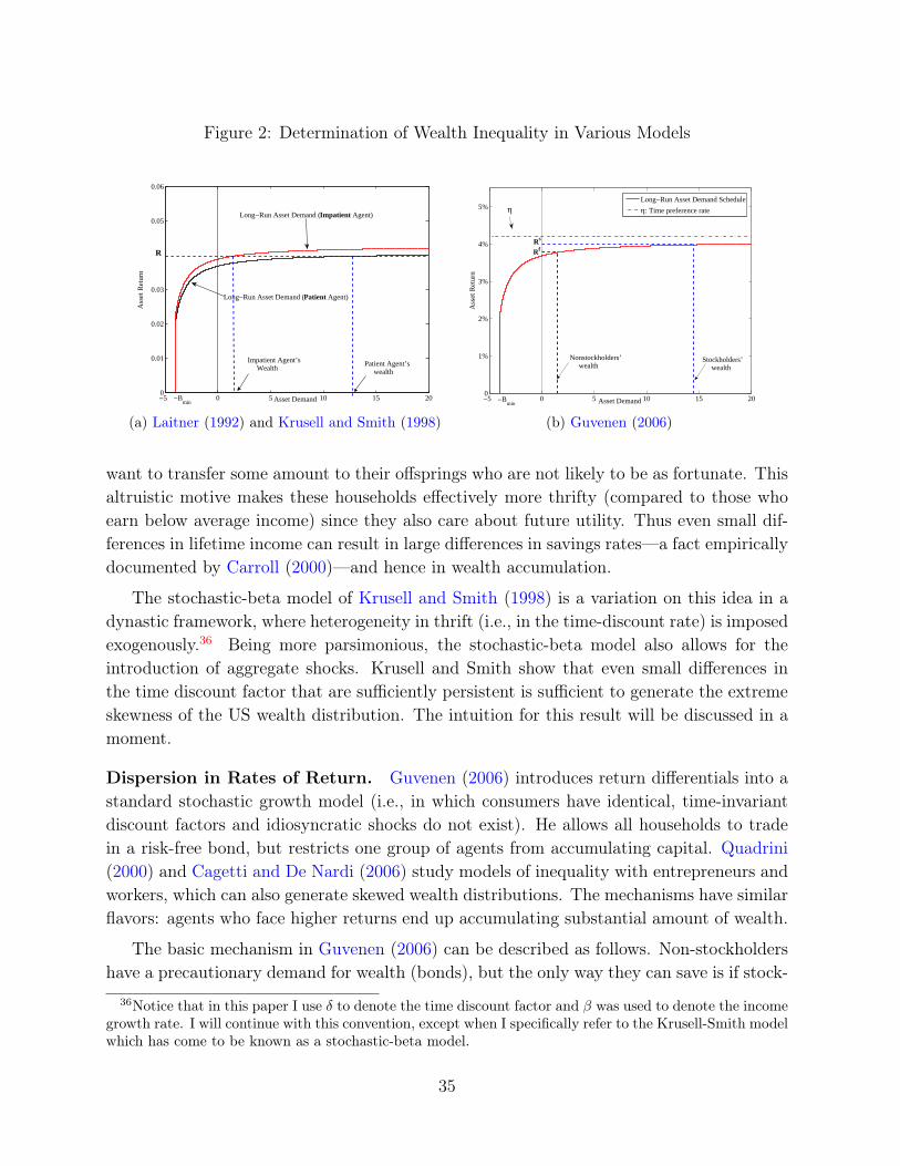
Figure 2: Determination of Wealth Inequality in Various Models

!5 0 5 10 15 200

0.01

0.02

0.03

0.05

0.06

Asset Demand

Ass

et R

eturn

Impatient Agent’s Wealth

Patient Agent’s wealth

!Bmin

Long!Run Asset Demand (Patient Agent)

Long!Run Asset Demand (Impatient Agent)

R

(a) Laitner (1992) and Krusell and Smith (1998)

!5 0 5 10 15 200

1%

2%

3%

4%

5%

Asset Demand

Ass

et R

eturn

Nonstockholders’ wealth

Stockholders’ wealth

Rs

Rf

!Bmin

Long!Run Asset Demand Schedule

!: Time preference rate!

(b) Guvenen (2006)

want to transfer some amount to their offsprings who are not likely to be as fortunate. Thisaltruistic motive makes these households effectively more thrifty (compared to those whoearn below average income) since they also care about future utility. Thus even small dif-ferences in lifetime income can result in large differences in savings rates—a fact empiricallydocumented by Carroll (2000)—and hence in wealth accumulation.

The stochastic-beta model of Krusell and Smith (1998) is a variation on this idea in adynastic framework, where heterogeneity in thrift (i.e., in the time-discount rate) is imposedexogenously.36 Being more parsimonious, the stochastic-beta model also allows for theintroduction of aggregate shocks. Krusell and Smith show that even small differences inthe time discount factor that are sufficiently persistent is sufficient to generate the extremeskewness of the US wealth distribution. The intuition for this result will be discussed in amoment.

Dispersion in Rates of Return. Guvenen (2006) introduces return differentials into astandard stochastic growth model (i.e., in which consumers have identical, time-invariantdiscount factors and idiosyncratic shocks do not exist). He allows all households to tradein a risk-free bond, but restricts one group of agents from accumulating capital. Quadrini(2000) and Cagetti and De Nardi (2006) study models of inequality with entrepreneurs andworkers, which can also generate skewed wealth distributions. The mechanisms have similarflavors: agents who face higher returns end up accumulating substantial amount of wealth.

The basic mechanism in Guvenen (2006) can be described as follows. Non-stockholdershave a precautionary demand for wealth (bonds), but the only way they can save is if stock-

36Notice that in this paper I use � to denote the time discount factor and � was used to denote the incomegrowth rate. I will continue with this convention, except when I specifically refer to the Krusell-Smith modelwhich has come to be known as a stochastic-beta model.

35

holders are willing to borrow. In contrast, stockholders have access to capital accumulation,so they could smooth consumption even if the bond market was completely shut down. Fur-thermore, non-stockholders’ asset demand is even more inelastic because they are assumedto have a lower elasticity of intertemporal substitution (consistent with empirical evidence)and therefore have a strong desire for consumption smoothing. Therefore, trading bondsfor consumption smoothing is more important for non-stockholders than it is for stockhold-ers. As a result, stockholders will only trade in the bond market if they can borrow ata low interest rate. This low interest rate in turn dampens non-stockholders’ demand forsavings further, and they end up with little wealth in equilibrium (and stockholders endup borrowing very little). Guvenen (2009b) shows that a calibrated version of this modeleasily generates the extremely skewed distribution of the relative wealth of stockholders tonon-stockholders in the US data.

Can we Tell them Apart? The determination of wealth inequality in the three modelsdiscussed so far can be explained using variations of a diagram used by Aiyagari (1994).The left panel of figure 2 shows how wealth inequality is determined in Laitner’s model and,given their close relationship, in the Krusell-Smith model. The top solid curve originatingfrom “�Bmin” plot the long-run asset demand schedule for the impatient agent; the bottomcurve is for the patient agent. A well-known feature of incomplete markets models is that theasset demand schedule is very flat for values of returns that are close to the time preferencerate, ⌘ (so � ⌘ 1/(1 + ⌘)). Thus, both types of individuals’ demand schedules asymptoteto their respective time preference rates (with ⌘patient < ⌘

impatient).37 If the equilibriumreturn (which must be lower than ⌘patient for an equilibrium to exist) is sufficiently closeto ⌘patient, the high sensitivity of asset demands to interest rates will generate substantialwealth inequality between the two types of agents.

Similarly, the right panel shows the mechanism in the limited participation model, whichhas a similar flavor. For simplicity, let us focus on the case where stockholders and non-stockholders have the same preferences and face the same portfolio constraints. We have⌘ > RS > Rf . Again, given the sensitivity of asset demand to returns near ⌘, even a smallequity premium generates substantial wealth inequality. It should be stressed, however,that a large wealth inequality is not a foregone conclusion in any of these models. If returnswere too low relative to ⌘, individuals would be on the steeper part of their demand curves,which could result in smaller differences in wealth holdings.

While the mechanics described here may appear quite similar for the three models,their substantive implications differ in crucial ways. For example, consider the effect ofeliminating aggregate shocks from all three models. In Guvenen (2006), there will beno equity premium without aggregate shocks and, consequently, no wealth inequality. In

37See, for example, Aiyagari (1994) and references therein. This result also holds when asset returns arestochastic (Chamberlain and Wilson (2000)).

36

Krusell and Smith (1998), wealth inequality will increase as the patient agent holds more ofthe aggregate wealth (and would own all the wealth if there were no idiosyncratic shocks). InLaitner (1992), wealth inequality will remain unchanged, since it is created by idiosyncraticlifetime income risk. These dramatically different implications suggest that one can devisemethods to bring empirical evidence to bear on the relevance of these different mechanisms.

Cagetti and De Nardi (2006). Cagetti and De Nardi (2006) introduce heterogeneityacross individuals in both work and entrepreneurial ability. Entrepreneurial firms operatedecreasing returns to scale production functions and higher entrepreneurial ability impliesa higher optimal scale. Because debt contracts are not perfectly enforceable due to limitedcommitment, business owners need to put some of their assets as collateral, a portion ofwhich would be confiscated in case of default. Entrepreneurs with very promising projectsthus have more to lose from default, which induces them to save more for collateral, borrowmore against it, and reach their larger optimal scale. The model is able to generate theextreme concentration of wealth at the top of the distribution (among households many ofwhom are entrepreneurs).

Although this model differs from the limited participation framework in many importantways, the differential returns to saving is a critical element for generating wealth inequality inboth models. This link could be important because many individuals in the top 1% and 5%of the US wealth distribution hold significant amounts of stocks but are not entrepreneurs(hold no managerial roles), which the Cagetti/De Nardi model misses. The opposite is alsotrue: many very rich entrepreneurs are not stockholders (outside of their own company)which does not fit well with Guvenen’s model (see Heaton and Lucas (2000) on the empiricalfacts about wealthy entrepreneurs and stockholders). The view that perhaps the very highwealth holdings of these individuals is driven by the higher returns that they enjoy—eitheras a stockholder or as an entrepreneur—can offer a unified theory of savings rate differences.

5.3 Wage and Earnings Inequality

Because the consumption-savings decision is the cornerstone of the incomplete marketsliterature, virtually every model has implications for consumption and wealth inequality.The same is not true for earnings inequality. Many models assume that labor supply isinelastic and the stochastic process for wages is exogenous, making the implications for wageand earnings inequality to be mechanical reflections of the assumptions of the model. Evenif labor supply is assumed to be endogenous, many properties of the earnings distribution(exceptions noted below) mimic those of the wage distribution. For things to get moreinteresting, it is the latter which needs to be endogenized as well.

In this section, I first review the empirical facts regarding wage inequality—both overthe life cycle and over time. These facts are useful to know for practitioners since they are

37

commonly used as exogenous inputs into incomplete markets models. Unless specificallymentioned, all the facts discussed here pertain to male workers, because the bulk of theexisting work is available consistently for this group.38 Second, I discuss models that attemptto endogenize wages and explain the reported facts and trends.

5.3.1 Inequality Over the Lifecycle

The main facts about the evolution of (within-cohort) earnings inequality over the lifecyclehave first been documented by Deaton and Paxson (1994) and shown in the left panel offigure 1. The same exercise has been repeated by numerous authors using different datasetsor time periods (among others, Storesletten et al. (2004b), Guvenen (2009a), Heathcote etal. (2010), and Kaplan (2010)). While the magnitudes differ somewhat, the basic fact thatwage and earnings inequality rise substantially over the life cycle is well-established.

One view is that this fact does not require an elaborate explanation, because wagesfollow a very persistent, perhaps permanent, stochastic process as implied by the RIPmodel. Thus, the rising lifecycle inequality is simply a reflection of the accumulation ofsuch shocks, which drives up the variance of log wages in a linear fashion (in the case ofpermanent shocks). I will continue to refer to this view as the RIP model because of itsemphasis on persistent “shocks.”39

An alternative perspective, which has received attention more recently, emphasizes sys-tematic factors—heterogeneity as opposed to random shocks. This view is essentially inthe same spirit as the HIP model of the previous section. But it goes one step further byendogenizing the wage distribution based on the human capital framework of Becker (1964)and Ben-Porath (1967) among others. In an influential paper, Huggett et al. (2006) havestudied the distributional implications of the standard Ben-Porath (1967) model by askingthe types of heterogeneity that one needs to introduce to generate patterns consistent withthe US data. They find that too much heterogeneity in initial human capital levels resultsin the counterfactual implication that wage inequality should fall over the lifecycle. Incontrast, heterogeneity in the learning ability generates rise in wage inequality consistentwith the data. A key implication of this finding is that the rise in wage inequality can begenerated without appealing to idiosyncratic shocks of any kind. Instead, it is the system-atic fanning out of wage profiles, resulting from different investment rates, that generatesrising inequality over the life cycle. Guvenen et al. (2009) and Huggett et al. (forthcoming)introduce idiosyncratic shocks into the Ben-Porath framework. Both papers find that het-erogeneous growth rates continue to play the dominant role for the rise in wage inequality.

38Some of the empirical trends discussed below also apply to women, while others do not. See Autor etal. (2008) for a comparative look at wage trends for males and females during the period.

39Of course, one can write deeper economic models which generates the the observation that wagesfollow a random walk process, such as the learning model of Jovanovic (1979) in a search and matchingenvironment, or the optimal contracts in the limited commitment model of Harris and Holmstrom (1982).

38

The Ben-Porath formulation is also central for wage determination in Heckman et al. (1998)and Kitao et al. (2008).

5.3.2 Inequality Trends Over Time

A well-documented empirical trend since the 1970s is the rise in wage inequality amongmale workers in the United States. This trend has been especially prominent above themedian of the wage distribution: for example, the log wage differential between the 90thand the 50th percentiles has been expanding in a secular fashion for the past four decades.The changes at the bottom have been more episodic, with the log 50-10 wage differentialstrongly expanding until late 1980s and then closing subsequently (see Autor et al. (2008)for a detailed review of the evidence). Acemoglu (2002) contains an extensive summaryof several related wage trends as well as a review of proposed explanations. Here I onlydiscuss the subset of papers that are more closely relevant for the incomplete markets macroliterature.

Larger Shocks or Increasing Heterogeneity? Economists’ interpretations of the risein wage inequality over the life cycle and over time are intimately related. The RIP view thatwas motivated by analyses of life-cycle wages was dominant in the 1980s and 1990s, so it wasnatural for economists to interpret the rise in wage inequality over time, through the samelens. Starting with Gottschalk and Moffitt (1994) and Moffitt and Gottschalk (1995), thistrend has been broadly interpreted as reflecting a rise in the variances of idiosyncratic shocks,either permanent or transitory (Meghir and Pistaferri (2004), Heathcote et al. (2008), etc.).This approach remains the dominant way to calibrate economic models that investigatechanges in economic outcomes from the 1970s to date.

However, some recent papers have documented new evidence that seems hard to reconcilewith the RIP view. The first group of papers revisit the econometric analyses of wage andearnings data. Among these, Sabelhaus and Song (2009, 2010) have used panel data fromSocial Security records covering millions of American workers, in contrast to the long list ofprevious studies that use survey data (e.g., the PSID).40 While this dataset has the potentialdrawback of under-reporting (because it is based on income reported to the IRS), it hasthree important advantages: (i) a much larger sample size (on the order of 50+ millionobservations, compared to at most 50,000 in the PSID), (ii) no survey response error, and(iii) no attrition. Sabelhaus and Song found that the volatility of annual earnings growthincreased during the 1970s, but that it declined monotonically during the 1980s and 1990s.Furthermore, applying the standard permanent-transitory decomposition as in Moffitt andGottschalk (1995) and Meghir and Pistaferri (2004) reveals that permanent shock variances

40These include, among others, Meghir and Pistaferri (2004), Dynan et al. (2007), Heathcote et al. (2008),and Solon and Shin (2011).

39

were stable and transitory shocks became smaller from 1980 into the 2000s. A separatestudy conducted by the Congressional Budget Office (2008), also using wage earnings fromSocial Security records from 1980 to 2003, reached the same conclusion.41 Finally, Kopczuket al. (2010) document (also using Social Security data) that both long-run and short-runmobility have stayed remarkably stable from 1960s into the 2000s. But this finding seemsdifficult to reconcile with Moffitt and Gottschalk (1995) and the subsequent literature thatfound permanent and transitory shock variances to have risen in different sub-periods from1970 to 2000s. If true, the latter would result in fluctuations in mobility patterns over thesesub-periods, which is not borne out in Kopczuk et al. (2010)’s analysis.

Another piece of evidence from income data is offered by Haider (2001), who estimated astochastic process for wages similar to the one in Moffitt and Gottschalk (1995) and others,but with one key difference. He allowed for individual-specific wage growth rates (HIP)and he also allowed for the dispersion of growth rates to vary over time. The stochasticcomponent is specified as an ARMA(1,1). With this more flexible specification, he foundno evidence of a rise in the variance of income shocks after 1970s, but instead found a largeincrease in the dispersion of systematic wage growth rates.

A second strand of the literature have studied the trends in labor market flows in theUnited States. These studies do not find any evidence of rising job instability or churning,which one might expect to see in conjunction with larger idiosyncratic shocks. In contrast,these studies document an across-the-board moderation in labor market flows. For example,Gottschalk and Moffitt (1999) focus on male workers between ages 20 and 62 and concludetheir analysis as follows:

[W]e believe that a consistent picture is emerging on changes in job stabilityand job security in the 1980s and 1990s. Job instability does not seem to haveincreased, and the consequences of separating from an employer do not seem tohave worsened.42

Shimer (2005, 2007) and Davis et al. (2010) extend this analysis to cover the 2000s and use avariety of datasets to reach the same conclusion. Further, both papers show that expandingthe sample of individuals to include women and younger workers shows a declining trendin labor market flows and increase in job security.

41Sabelhaus-Song attribute the reason why some earlier studies found rising variances of wage shocks(e.g., Moffitt and Gottschalk (2008)) to the inclusion of individuals with self-employment income and thosewho earn less than the Social Security minimum. Even though there are few of these households, they showthat they make a big difference in the computed statistics. Similarly, Solon and Shin (2011, p. 978-980)use PSID data and also do not find a trend in the volatility of wage earnings changes during the 1980s and1990s. They argue that the increasing volatility found in earlier studies, such as Dynan et al. (2007) seemsto be coming from the inclusion of some auxiliary types of income (from business, farming, etc) whosetreatment has been inconsistent in the PSID over the years.

42They also say, “Almost all studies based on the various Current Population Surveys (CPS) supplements...show little change in the overall separation rates through the early 1990s.”

40

Taking Stock. To summarize, the seeming consensus of the 1990s—that rising wageinequality was driven by an increase in idiosyncratic shock variances—is being challengedby a variety of new evidence, some of which from data sets many orders of magnitudelarger than the surveys used in previous analyses. In addition, the evidence from labormarket flows described above—while perhaps more indirect—raises questions about thesources of larger idiosyncratic shocks in a period where labor market transitions seem tohave moderated. Although, it would be premature to conclude that the alternative viewis the correct one—more evidence is needed to reach a definitive conclusion. Having saidthat, if this alternative view is true, and income shock variances have not increased, thisnew “fact” would require economists to rethink a variety of explanations put forward forvarious trends, which took as given a rise in shock variances during this period.

6 Heterogeneity with Aggregate Shocks

Krusell and Smith (1998) added two elements to the basic Aiyagari framework. First theyintroduced aggregate technology shocks. Second, they assumed that the cumulative discountfactor at time t (which was assumed to be �t before), now follows the stochastic process�t

=

˜��t�1

, where ˜� is a finite-state Markov chain. The stochastic evolution of the discountfactors within a dynasty captures some elements of an explicit overlapping-generationsstructure with altruism and less than perfect correlation in genes between parents andchildren, as in Laitner (1992). With this interpretation in mind, the evolution of ˜� iscalibrated so that the average duration of any particular value of the discount factor isequal to the lifetime of a generation. (Krusell and Smith (1997) study a version of thismodel where consumers are allowed to hold a risk-free bond in addition to capital.)

The specifics of the model are as follows. There are two types of shocks: (i) idiosyn-cratic employment status: (✏

e

, ✏u

) ⌘ (employed, unemployed); (ii) aggregate productivity:(z

g

, zb

) ⌘ (expansion, recession). Employment status and aggregate productivity jointlyevolve as a first order Markov process. Assume that ✏ is i.i.d. conditional on z, so thefraction of employed workers (and hence l) only depends on z. Competitive markets imply

w(K,L, z) = (1� ↵)z(K/L)�↵, and r(K,L, z) = ↵z(K/L)↵. (12)

Finally, the entire wealth distribution, which I denote with � is a state variable for thismodel and let �0

= H(�, z, z0) denote its endogenous transition function (or law of motion).

6.1 Krusell-Smith Algorithm

A key equilibrium object in this class of models is the law of motion, H. In principle,computing this object is a formidable task since the distribution of wealth is infinite-

41

dimensional. Krusell and Smith (1997, 1998) show, however, that this class of models,when reasonably parameterized, exhibits “approximate aggregation”: loosely speaking, topredict future prices consumers need to forecast only a small set of statistics of the wealthdistribution rather than the entire distribution itself. This result makes it possible to usenumerical methods to analyze this class of models. Another key feature of the Krusell-Smithalgorithm is that it solves the model by simulating it. Specifically, the basic version of thealgorithm works as follows:

1. Approximate � with a finite number (I) of moments. (H reduces to a function map-ping the I moments today into the I moments tomorrow depending on z today.)

• We will start by selecting one moment—the mean—so I = 1.43

2. Select a family of functions for H. I will choose a log-linear function following Kruselland Smith.

V (k,✏ ;�, z) = max

c,k

0

hU(c) + �E[V (k

0, ✏

0;�

0, z

0)| z,✏ ]

i

c+ k0= w(K,L, z)⇥ l ⇥ ✏+ r(K,L, z)⇥ k, k0 � 0

logK 0= a

0

+ a1

logK for z = zb

logK 0= b

0

+ b1

logK for z = zg

3. Make an (educated) initial guess about (a0

, a1

, b0

, b1

) ) yields initial guess for H0

.Make also an initial guess for �

0

.

4. Solve the consumer’s dynamic program. Using only the resulting decision rules, sim-ulate {k

n,t

}N,T

n=1,t=1

for (N, T ) large.

5. Update H by estimating (where eK =

1

N

PN

n=1

kn

) :

log

eK 0= a

0

+ a1

log

eK for z = zb

log

eK 0= b

0

+ b1

log

eK for z = zg

6. Iterate on 4-5, until the R2 of this regression is “sufficiently high” and the forecastvariance is “small.”

• If accuracy remains insufficient, go back to step 1 and increase I.43When we add more moments, we do not have to proceed as mean, variance, skewness, and so on. We

can include, say, the wealth holdings of the top 10 percent of population, mean- to-median wealth ratio,etc.

42

6.2 Details

Educated Initial Guess. As with many numerical methods, a good initial guess is criti-cal. More often than not, the success or failure of a given algorithm will depend on the initialguess. One idea (used by Krusell and Smith) is to first solve a standard representative-agentRBC model with the same parameterization. Then estimate the coefficients (a

0

, a1

, b0

, b1

)

using capital series simulated from this model to obtain an initial guess for step 1 above.44

More generally, a good initial guess can often be obtained by solving a simplified versionof the full model. Sometimes this simplification involves ignoring certain constraints, some-times by shutting down certain shocks, and so on.

Discretizing an AR(1) Process. Oftentimes, the exogenous driving force in incompletemarkets models is assumed to be generated by an AR(1) process, which is discretized andconverted into a Markov chain. One popular method for discretization is described inAiyagari (1993) and has been used extensively in the literature. However, an alternativemethod due to Rouwenhorst (1995) (and which received far less attention until recently) isfar superior in the quality of the approximation that it provides, especially when the processis very persistent, which is often the case. Moreover, it is very easy to implement. Kopeckyand Suen (2010) and Lkhagvasuren and Galindev (2010) provide comprehensive comparisonsof different discretization methods, which reveal the general superiority of Rouwenhorst(1995)’s method. They also show how this method can be extended to discretize moregeneral processes.

Non-Trivial Equilibrium Pricing Function. One simplifying feature of Krusell andSmith (1998) is that equilibrium prices (wages and interest rates) are determined triviallyby the marginal product conditions (12). Thus they depend only on the aggregate capitalstock and not on its distribution. Some models do not have this structure—instead pricingfunctions must be determined by equilibrium conditions—such as market-clearing or zero-profit conditions—that explicitly depend on the wealth distribution. This would be thecase, for example, if a household bond is traded in the economy. Its price must be solvedfor using market clearing condition, which is a challenging task. Moreover, if there isan additional asset, such as a stock, two prices must be determined simultaneously, andthis must be done in such a way that avoids providing arbitrage opportunities—along theiterations of the solution algorithm. Otherwise, individuals’ portfolio choices will go haywire(in an attempt to take advantage of perceived arbitrage), wreaking havoc with the solutionalgorithm. Krusell and Smith (1997) solved such a model and proposed an algorithm totackle these issues. I refer the interested reader to that paper for details.

44Can’t we update H without simulating? Yes we can. den Haan and Rendahl (2009) propose a methodwhere they use the policy functions for capital holdings and integrate them over distribution ⇤(k,✏ ) ofhouseholds across capital and employment status: K

0= Hj(K, z) =

Rk

0

j(k,✏ ;�, z)d⇤(k,✏ ). This works wellwhen the decision rules are parameterized in a particular way. See den Haan and Rendahl (2009).

43

Checking for Accuracy of Solution. Many studies with aggregate fluctuations andheterogeneity use two simple criteria to asses the accuracy of the law of motion in theirlimited information approximation. If agents are using the law of motion

logK 0= ↵

1

+ ↵2

z + ↵3

logK + u (13)

a perfectly solved model should find u = 0. Thus, practitioners will continue to solve themodel until either the R2 of this regression is larger than some minimum or �

u

falls belowsome threshold (step 6 in the algorithm above).

However, one should not rely solely on R2 and �u

. There are at least three reasons forthis (den Haan (2010)). First, both measures average over all periods of the simulation.Thus, infrequent but large deviations from the forecast rule can be hidden in the average.These errors may be very important to agents and their decision rule. For example, thethreat of a very large recession may increase buffer stock saving, but the approximationmay understate the movement of capital in such a case. Second, and more importantly,these statistics only measure one-step ahead forecasts. The regression only considers thedynamics from one period to the next, so errors are only the deviations between the actualnext-period capital and the expected amount in the next period. This misses potentiallylarge deviations between the long-term forecast for capital and its actual level. Aware ofthis possibility, Krusell and Smith (1998) also checked the R2 for forecasting prices 25 yearsahead (100 model periods) and found it to be extremely high as well! (They also check themaximum error in long-term forecasts, which was very small.) Third, R2 is scaled by theLHS of the regression. An alternative is to check the R2 of:

logK 0 � logK = ↵1

+ ↵2

z + (↵3

� 1) logK

As a particularly dramatic demonstration, den Haan (2010) uses a savings decision rulethat solves the Krusell and Smith (1998) model, simulates it for T periods and estimates alaw of motion in the form of equation (13). He then manipulates ↵

1

,↵3

such that T�1

Put

=

0 but the R2 falls from 0.9999 to 0.999 and then 0.99. This has economically meaningfulconsequences: the time series standard deviation of the capital stock simulated from theperturbed version of equation (13) falls to 70% and then 46% of the true figure.

Finally, den Haan (2010) proposes a useful test that begins with the approximated lawof motion

logK 0= ↵̂

1

+ ↵̂2

z + ↵̂3

logK + u (14)

to generate a sequence of realizations of { eKt+1

}Tt=0

and then compare these to the sequencegenerated by aggregating from decision rules, the true law of motion. Because { eK

t+1

}Tt=0

is obtained by repeatedly applying Equation (14) starting from eK0

, errors can accumulate.This is important because in the true model, today’s choices depend upon expectations

44

about the future state, which in turn depends upon the future’s future expectations andso errors cascade. To systematically compare eK

t

to Kt

, den Haan proposes an “essentialaccuracy plot.” For a sequence of shocks (not those originally used when estimating ↵’s tosolve the model) generate a sequence of eK

t

and Kt

. One can then compare moments of thetwo simulated sequences. The “main focus” of the accuracy test are the errors calculatedby eu

t

= | log eKt

� logKt

|, whose maximum should be made close to zero.

Prices Are More Sensitive Than Quantities. The accuracy of the numerical solutionbecomes an even more critical issue if the main focus of analysis is (asset) prices ratherthan quantities. This is because prices are much more sensitive to approximation errors(see, e.g., Christiano and Fisher (2000), and Judd and Guu (2001)). The results in Chris-tiano and Fisher (2000) are especially striking. These authors compare a variety of differentimplementations of the “parameterized expectations” method and report the approximationerrors resulting from each. For the standard deviation of output, consumption, and invest-ment (i.e., “quantities”) the approximation errors range from less than 0.1% of the true valueto 1-2% in some cases. For the stock and bond return and the equity premium, the errorsregularly exceed 50% and are greater than 100% in several cases. The bottom-line is thatthe computation of asset prices require extra care.

Pros and Cons. An important feature of the Krusell-Smith method is that it is a “local”solution around the stationary recursive equilibrium. In other words, this method relieson simulating a very long time series of data (e.g., capital series) and making sure thatafter this path has converged to the ergodic set, the predictions of agents are accurate forbehavior inside that set. This has some advantages and some disadvantages. On advantageis the efficiency gain compared to solving a full recursive equilibrium, which enforces theequilibrium conditions at every point of a somewhat arbitrary grid, regardless of whetheror not a given state is ever visited in the stationary equilibrium.

One disadvantage is that if you take a larger deviation—say by setting K0

to a valuewell below the steady state value—your “equilibrium functions” are likely to be inaccurate,and the behavior of the solution may differ significantly from the true solution. Why shouldwe care about this? Suppose you solve your model then want to study a policy experimentwhere you eliminate taxes on savings. You would need to write a separate program fromthe “transition” between the two stationary equilibria. Instead, if you solve for the fullrecursive equilibrium over a grid that contains both the initial and final steady states, youwould not need to do this. However, solving for the full equilibrium is often much harderand, therefore, is often “over-kill.”

An Alternative to Krusell-Smith: Tracking History of Shocks. Some models havefew exogenous state variables, but a large number of endogenous states. In such cases, usinga formulation that keeps track of all these state variables can make the numerical solution

45

extremely costly or even infeasible. An alternative method begins with the straightforwardobservation that all current endogenous state variables are nothing more than functions ofthe infinite history of exogenous shocks. So, one could replace these endogenous states withthe infinite history of exogenous states. Moreover, many models turn out to have “limitedmemory” in the sense that only the recent history of shocks matters in a quantitativelysignificant way, allowing us to only track a truncated history of exogenous states. The firstimplementation of this idea I have been able to find is in Veracierto (1997), who studied amodel with plant-level investment irreversibilities, which give rise to S-s type policies. Heshowed that it is more practical to track a short history of the S-s thresholds instead of thecurrent-period endogenous state variables.

As another example, consider an equilibrium model of the housing market where theonly exogenous state is the interest rate, which evolves as a Markov process. Dependingon the precise model structure, the individual endogenous state variables can include themortgage debt outstanding, the time-to-maturity of the mortgage contract, etc., and theaggregate endogenous state can include the entire distribution of agents over the individualstates. This is potentially an enormously large state space! Arslan (2011) successfully solvesa model of this sort with realistic fixed-rate mortgage contracts, a lifecycle structure, andstochastic interest rates, using 4 lags of interest rates. Other recent examples that employthis basic approach include Lustig and Chien (2010) who solve an asset pricing model withaggregate and idiosyncratic risk in which agents are subject to collateral constraints arisingfrom limited commitment, and Lorenzoni (2009) who solves a business cycle model withshocks to individuals’ expectations. In all these cases, tracking a truncated history turnsout to provide computational advantages over choosing endogenous state variables thatevolve in a Markovian fashion. One advantage of this approach is that it is often less costlyto add an extra endogenous state variable relative to the standard approach, because thesame number of lags may still be sufficient. One drawback is that if the Markov processhas many states or the model has long memory, the method may not work as well.

7 When Does Heterogeneity Matter for Aggregates?

As noted earlier, Krusell and Smith (1998) report that the time series behavior of theaggregated incomplete markets model, by and large, looks very similar to the correspondingrepresentative-agent model. A similar result was reported in Rios-Rull (1996). However,it is important to interpret these findings correctly and to not overgeneralize them. Forexample, even if a model aggregates exactly, modeling heterogeneity can be very importantfor aggregate problems. This is because the problem solved by the representative agentcan look dramatically different from the problem solved by individuals (for example, havevery different preferences). Here, I discuss some important problems in macroeconomics

46

where introducing heterogeneity yields conclusions quite different from a representative-agent model.

7.1 The Curse of Long Horizon

It is useful to start by discussing why incomplete markets do not matter in many models.Loosely speaking, this outcome follows from the fact that a long horizon makes individuals’savings function approximately linear in wealth (i.e., constant MPC out of wealth). As wesaw in Section 2, the exact linearity of savings rule delivered exact demand aggregationin both Gorman (1961) and Rubinstein (1974)’s theorems. As it turns out, even withidiosyncratic shocks, this near-linearity holds for wealth levels that are not immediately nearborrowing constraints. Thus, even though markets are incomplete, redistributing wealthwould matter little, and we have something that looks like demand aggregation!

Is there a way to get around this result? It is instructive to look at a concrete example.Mankiw (1986) was one of the first papers in the literature on the equity premium puzzleand one that gave prominence to the role of heterogeneity. Mankiw (1986) showed that, in atwo-period model with incomplete markets and idiosyncratic risk of the right form, one cangenerate an equity premium as large as desired. However, researchers who followed up onthis promising lead (Telmer (1993), Heaton and Lucas (1996), and Krusell and Smith (1997))quickly came to a disappointing conclusion: once agents in these models are allowed to livefor multiple periods, trading a single risk-free asset yields sufficient consumption insurance,which in turn results in a tiny equity premium.

This result—that a sufficiently long horizon can dramatically weaken the effects of in-complete markets—is quite general. In fact, Levine and Zame (2002) proved that in asingle good economy with no aggregate shocks if: (i) idiosyncratic income shocks follow aMarkov process, (ii) marginal utility is convex, and (iii) all agents have access to a singlerisk-free asset, then as individual’s subjective time discount factor (�) approaches unity,then incomplete markets allocations (and utilities) converge to those from a complete mar-kets economy with the same aggregate resources. Although Levine and Zame’s result istheoretical for the limit of such economies (as � ! 1), it still sounds a cautionary noteto researchers building incomplete markets models: unless shocks are extremely persistentand/or individuals are very impatient, these models are unlikely to generate results muchdifferent from a representative-agent model.

Constantinides and Duffie (1996) have shown one way to get around the problem of a longhorizon, which is also consistent with the message of Levine-Zame’s theorem. Essentiallythey assume that individuals face permanent shocks, which eliminates the incentives tosmooth such shocks. Therefore, they behave as if they live in a static world and choose notto trade. Constantinides and Duffie also revive another feature of Mankiw (1986)’s model:idiosyncratic shocks must have larger variance in recessions (i.e., countercyclical variances)

47

to generate a large equity premium. With these two features, they show that Mankiw’soriginal insight can be made to work once again in an infinite horizon model. Storeslettenet al. (2007) found that a calibrated model along the lines suggested by Constantinides andDuffie can generate about 1/4 of the equity premium observed in the US data.

The bottom line is that, loosely speaking, if incomplete markets matter in a modelmainly through its effect on the consumption-saving decision, a long horizon can signifi-cantly weaken the bite that incomplete markets has. With a long enough horizon, agentsaccumulate sufficient wealth and end up on the nearly linear portion of their savings func-tion, delivering results not far from a complete markets model. This is also the upshot ofKrusell and Smith (1998)’s analysis.

7.2 Examples Where Heterogeneity Does Matter

There are many examples in which heterogeneity does matter for aggregate phenomena.Here, I review some examples.

First, aggregating heterogeneous-agent models can give rise to preferences for the repre-sentative agent that may have nothing to do with the preferences in the underlying model.A well-known example of such a transformation was present in the early works of Hansen(1985) and Rogerson (1988), who showed that in a model in which individuals have no in-tensive margin of labor supply (i.e., zero Frisch labor supply elasticity), one can aggregatethe model to find that the representative agent has linear preferences in leisure (i.e., infiniteFrisch elasticity!). This conclusion challenges one of the early justifications for buildingmodels with micro-foundations, which was to bring evidence from micro data to bear onthe calibration of macro models. In an excellent survey paper, Browning et al. (1999)sounded an early cautionary note, giving several examples where this approach is fraughtwith danger.

Building on the earlier insights of Hansen and Rogerson, Chang and Kim (2006) con-struct a model in which aggregate labor-supply elasticity depends on the reservation-wagedistribution in the population. The economy is populated by households (husband andwife) who each supply labor only along the extensive margin: they either work full time orstay home. Workers are hit by idiosyncratic productivity shocks, causing them to move inand out of the labor market. The aggregate labor-supply elasticity of such an economy isaround 1, greater than a typical micro estimate and much greater than the Frisch elasticityone would measure at the intensive margin (which is zero) in this model. The model thusprovides a reconciliation between the micro and macro labor-supply elasticities. In a sim-ilar vein, Chang et al. (2010) show that preference shifters that play an important role indiscussions of aggregate policy are not invariant to policies if they are generated from theaggregation of a heterogeneous-agent model. Such a model also generates “wedges” at theaggregate level that do not translate into any well-defined notion of preference shifters at

48

the micro level.45 Finally, Erosa et al. (2009) build a lifecycle model of labor supply, bycombining and extending the ideas introduced in earlier papers, such as Chang and Kim(2006) and Rogerson and Wallenius (2009). Their goal is to build a model with empiricallyplausible patterns of hours over the life cycle and examine the response elasticities of laborsupply to various policy experiments.

In another context, Guvenen (2006) asks why macroeconomic models in the RBC tra-dition typically need to assume a high elasticity of intertemporal substitution (EIS) toexplain output and investment fluctuations, whereas Euler equation regressions (such asin Hall (1988) and Campbell and Mankiw (1990)) that use aggregate consumption dataestimate a much smaller EIS (close to zero) to fit the data. He builds a model with twotypes of agents who differ in their EIS. The model generates substantial wealth inequalityand much smaller consumption inequality, both in line with the US data. Consequently,capital and investment fluctuations are mainly driven by the rich (who hold almost all thewealth in the economy) and thus reflect the high EIS of this group. Consumption fluctua-tions, on the other hand, reflect an average that puts much more weight on the poor’s EIS,who contribute significantly to aggregate consumption. Thus, a heterogeneous agent modelis able to explain aggregate evidence that a single representative-agent model has troublefitting.

In an asset pricing context, Constantinides and Duffie (1996), Chan and Kogan (2002)and Guvenen (2011) show a similar result for risk aversion. Constantinides and Duffie (1996)show theoretically how the cross-sectional distribution of consumption in a heterogeneous-agent model gets translated into a higher risk aversion for the representative agent. Guve-nen (2011) shows that in a calibrated model with limited stock market participation thatmatches several asset pricing facts, the aggregate risk aversion is measured to be as highas 80, when the individuals’ risk aversion is only 2. These results as well as the papersdiscussed above confirm and amplify the concerns originally highlighted by Browning et al.(1999). The conclusion is that researchers must be very careful when using micro evidenceto calibrate representative-agent models.

8 Computation and Calibration

Because of their complexity, the overwhelming majority of models in this literature aresolved on a computer using numerical methods.46 Thus, I now turn to a discussion ofcomputational issues that researchers often have to confront when solving models withheterogeneity.

45See Chari et al. (2007) for the definition of business cycle wedges.46There are few examples of analytical solutions and theoretical results established with heterogeneous-

agent models. See, e.g., Constantinides and Duffie (1996), Heathcote et al. (2007), Wang (2009), Guvenenand Kuruscu (forthcoming), and Rossi-Hansberg and Wright (2007).

49

8.1 Calibration and Estimation: Avoid Local Search

Economists often need to minimize an objective function of multiple variables that haslots of kinks, jaggedness, and deep ridges. Consequently, the global minimum is oftensurrounded by a large number of local minima. A typical example of such a problem ariseswhen a researcher tries to calibrate several structural parameters of an economic modelby matching some data moments. Algorithms based on local optimization methods (e.g.,Newton-Raphson style derivative-based methods or Nelder-Mead simplex style routines)very often get stuck in local minima, because the objective surface is typically very rough(non-smooth).

It is useful to understand some of the sources of this roughness. For example, linear in-terpolation that is often used in approximating value functions or decision rules generates aninterpolated function that is non-differentiable (i.e., have kinks) at every knot point. Sim-ilarly, problems with (borrowing, portfolio, etc.) constraints can create significant kinks.Because researchers use a finite number of individuals to simulate data from the model(to compute moments) a small change in the parameter value (during the minimizationof the objective) can move some individuals across the threshold—from being constrainedto unconstrained or vice versa—which can cause small jumps in the objective value. Andsometimes, the moments that the researcher decides to match would be inherently discon-tinuous in the underlying parameters (with a finite number of individuals), such as themedian of a distribution (e.g., wealth holdings). Further compounding the problems, ifthe moments are not jointly sufficiently informative about the parameters to be calibrated,the objective function would be flat in certain directions. As can be expected, trying tominimize a relatively flat function with lots of kinks, jaggedness, and even small jumps, canbe a very difficult task indeed.47

While the algorithm described here can be applied to the calibration of any model, it isespecially useful in models with heterogeneous agents—since such models are time consum-ing to solve even once, an exhaustive search of the parameter space becomes prohibitivelycostly (which could be feasible in simpler models).

8.2 A Simple Fully Parallelizable Global Optimization Algorithm

Here, I describe a global optimization algorithm that I regularly use for calibratingmodels and I have found it to be very practical and powerful. It is relatively straightforward

47One simple, but sometimes overlooked, point is that when minimizing an objective function of momentsto calibrate a model, one should use the same “seeds” for the random elements of the model that are usedto simulate the model in successive evaluations of the objective function. Otherwise, some of the changein objective value will be due to the inherent randomness in different draws of random variables. This cancreate significant problems with the minimization procedure.

50

to implement, yet allows full parallelization across any number of CPU cores as well as acrossany number of computers that are connected to the Internet. It requires no knowledge ofMPI, OpenMP, or related tools, and no knowledge of computer networking other than usingsome commercially available synchronization tools (such as DropBox, SugarSync, etc.).

A broad outline of the algorithm is as follows. As with many global algorithms, thisprocedure combines a global stage with a local search stage that is restarted at variouslocations in the parameter space. First, we would like to search the parameter space asthoroughly as possible, but do so in as efficient a way as possible. Thoroughness is essentialbecause we want to be sure that we found the true global minimum, so we are willing tosacrifice some speed to ensure this. The algorithm proceeds by taking an initial startingpoint (chosen in a manner described momentarily) and conducting a local search from thatpoint on until the minimization routine converges as specified by some tolerance. For localsearch, I typically rely on the Nelder-Mead’s downhill simplex algorithm because it doesnot require derivative information (that may be inaccurate given the approximation errorsin the model’s solution algorithm).48 The minimum function value as well as the parametercombination that attained that minimum are recorded in a file saved on the computer’s harddisk. The algorithm then picks the next “random” starting point and repeats the previousstep of local minimization. The results are then added to the previous file, which recordsall the local minima found up to that point.

Of course, the most obvious algorithm would be to keep doing a very large number ofrestarts of this sort and take the minimum of all the minima found in the process. Butthis would be very time consuming and would not be particularly efficient. Moreover, inmany cases, the neighborhood of the global minimum can feature many deep ridges andkinks nearby, which requires more extensive searching near the global minimum, whereasthe proposed approach would devote as much time to points far away from the true globalminimum as to the points near it. Further, if the starting points are chosen literally ran-domly, this would also create potentially large efficiency losses, because these points have anon-negligible chance of falling near points previously tried. Because those areas have beenpreviously searched, devoting more time is not optimal.

A better approach is to use “quasi-random” numbers to generate the starting points.Quasi-random numbers (also called Low-discrepancy sequences) are sequences of determin-istic numbers that spread to any space in the maximally separated way. They avoid thepitfall of random draws that may end up being too close to each other. Each draw in thesequence “knows” the location of previous points drawn and attempts to fill the gaps asevenly as possible.49 Among a variety of sequences proposed in the literature, the Sobol’

48An alternative that can be much faster but requires a bit more tweaking for best performance is thetrust region method of Zhang et al. (2010) that builds on Powell (2009)’s BOBYQA algorithm.

49Another common application of low-discrepancy sequences is in quasi-Monte Carlo integration, wherethey have been found to improve time-to-accuracy by several orders of magnitude.

51

sequence is generally viewed to be superior in most practical applications, having a veryuniform filling of the space (i.e., maximally separated) even for a small number of pointsdrawn as well as a very fast algorithm that generates the sequence.50

Next, how do we use the accumulated information from previous restarts? As suggestedby genetic algorithm heuristics, I combine information from previous best runs to adaptivelydirect the new restarts to areas that appear more promising. This is explained further below.Now for the specifics of the algorithm.

Let p be a J-dimensional parameter vector with generic element pj, j = 1, .., J.

• Step 0. Initialization:

1. Determine bounds for each parameter, outside of which the objective functionshould be set to a high value.

2. Generate a sequence of Sobol’ numbers with a sequence length of Imax

(the maxi-mum anticipated number of restarts in the global stage). Set the global iterationnumber i = 1.

• Step 1. Global stage:

1. Draw the ith (vector) value in the Sobol’ sequence: si

.

2. If i > 1, open and read from the text file “saved_parameters.dat” the functionvalues (and corresponding parameter vectors) of previously found local minima.Denote the lowest function value found as of iteration i � 1 as f low

i�1

and thecorresponding parameter vector as plow

i�1

.

3. Generate a starting point for the local stage as follows:

– If i < Imin

(< Imax

) then use si

as the initial guess: Si

= si

. Here, Imin

is thethreshold below which we use fully quasi-random starting points in the globalstage.

– If i � Imin, take the initial guess to be a convex combination of si

and theparameter value that generated the best local minima so far: S

i

= (1 � ✓i

)si

+

✓plow

i�1

. The parameter ✓i

2 [0, ✓] with ✓ < 1, and increases with i. For example,I found that a convex increasing function, such as ✓

i

= min[✓, (i/Imax

)

2], workswell in some applications. An alternative heuristic is given later.

– As ✓i

is increased local searches are restarted from a narrower part of the param-eter space that yielded the lowest local minima before.

50In a wide range of optimization problems, Liberti and Kucherenko (2005) and Kucherenko and Sytsko(2005) find that Sobol’ sequences outperforms Holton sequences, both in terms of computation time andprobability of finding the global optimum. The Holton sequence is particularly weak in high dimensionalapplications.

52

• Step 2: Local stage:

– Using Si

as a starting point, use the downhill simplex algorithm to search for alocal minimum. (For the other vertices of the simplex, randomly draw startingpoints within the bounds of the parameter space).

– Stop when either (i) a certain tolerance has been achieved, (ii) function values donot improve more than a certain amount, or (iii) the maximum iteration numberis reached.

– Open saved_parameters.dat and record the local minimum found (functionvalue and parameters).

• Step 3. Stopping Rule:

– Stop if the termination criterion described below is satisfied. If not go to step 1.

Termination Criterion. One useful heuristic criterion relies on a Bayesian procedurethat estimates the probability that the next local search will find a new local minimumbased on the rate at which new local minima have been located in past searches. Moreconcretely, if W different local minima have been found after K local searches started froma set of uniformly distributed points, then the expectation of the number of local minima is

Wexp = W (K−1)/(K−W−2)

provided that K > W + 2. The searching procedure is terminated if Wexp < W + 0.5. Theidea is that, after a while of searching, if subsequent restarts keep finding one of the thesame local minima found before, the chances of improvement in subsequent searches is notworth the additional time cost. Although this is generally viewed as one of the most reliableheuristics, care must be applied as with any heuristic.

Notice also that Wexp can be used to adaptively increase the value of ✓i

in the globalstage (Step 1(3) above). The idea is that as subsequent global re-starts do not yield anew local minimum with a high enough probability, it is time to narrow down the searchand further explore areas of promising local minima. Because jaggedness and deep ridgescause local search methods to often get stuck, we want to explore promising areas morethoroughly.

One can improve upon this basic algorithm in various ways. I am going to mention afew that seem worth exploring.

53

Refinements: Clustering and Pre-testing. First, suppose that in iteration k, theproposed starting point S

k

ends up being “close” to one of the previous minima, say plow

n

,for n < k. Then it is likely that the search starting from S

k

will end up converging to plow

n

.

But then we have wasted an entire cycle of local search without gaining anything. To preventthis, one heuristic (called “clustering methods”) proceeds by defining a “region of attraction”(which is essentially a J-dimensional ball centered) around each one of the local minimafound so far.51 Then the algorithm would discard a proposed re-starting point if it falls intothe region attraction of any previous local minima. Because the local minimization stage isthe most computationally intensive step, this refinement of restarting the local search onlyonce in a given region of attraction can result in significant computational gains. Extensivesurveys of clustering methods can be found in Rinnooy Kan and Timmer (1987a,b).

Second, one can add a “pre-test” stage where N points from the Sobol’ sequence areevaluated before any local search (i.e., in Step 0 above), and only a subset of N⇤ < N

points with lowest objective values are used as seeds in the local search. The remainingpoints as well as regions of attraction around it are ignored as not promising. Notice thatwhile this stage can improve speed, it trades off reliability in the process.

Narrowing Down the Search Area. The file saved_parameters.dat contains a lot ofuseful information gathered in each iteration to the global stage, which can be used moreefficiently as follows. As noted, the Nelder-Mead algorithm requires J +1 candidate pointsas inputs (the vertices of the J-dimensional simplex). One of these points is given by S

i

,chosen as described above; the other vertices were drawn randomly. But as we accumulatemore information with every iteration on the global stage, if we keep finding local minimathat seem to concentrate in certain regions, it makes sense to narrow the range of valuesfrom which we pick the vertices. One way to do this is as follows: After a sufficiently largenumber of re-starts have been completed, rank all the function values and take the lowestx% of values (e.g., 10% or 20%). Then for each dimension, pick the minimum (call pjmin) andmaximum parameter value (call pjmax) within this set of minima. Then to generate vertices,take randomly sampled points between pjmin and pjmax in each dimension j. This allows thesimplex algorithm to search more intensively in a narrower area, which can improve resultsvery quickly when there are ridges or jaggedness in the objective function that makes thealgorithm to get stuck.

51While different formulas have been proposed for determining the optimal radius, these formulas containsome undetermined coefficients which makes them less than useful in real life applications.

54

8.3 Parallelizing the Algorithm

The algorithm can be parallelized in a relatively straightforward manner.52 The basic ideais to let each CPU core perform a separate local search in a different part of the parameterspace, which is a time-consuming process. If we can do many such searches simultaneously,we can speed up the solution dramatically. One factor that makes parallelization simple isthat fact that the CPU cores do not need to communicate with each other during the localsearch stage. In-between the local stages, each CPU core will contribute its findings (thelast local minimum it found along with the corresponding parameter vector) to the collectivewisdom recorded in saved_parameters.dat and also get the latest updated informationabout the best local minimum found so far from the same file. Thus, as long as all CPU coreshave access to the same copy of the file saved_parameters.dat, parallelization requires nomore than a few lines for housekeeping across CPUs. Here are some more specifics.

Suppose that we have a workstation with N CPU cores (for example, N = 4, 6, or 12).The first modification we need to make is to change the program to distinguish betweenthe different “copies” of the code, running on different CPU cores. This can be done bysimply having the program ask the user (only once, upon starting the code) to input aninteger value, n, between 1 and N , which uniquely identifies the “sequence number” of theparticular instance of the program running. Then open N terminal windows and launch acopy of the program in each window. Then for each one, enter a unique sequence numbern = 1, 2..., N .

Upon starting, each program will first simulate the same quasi-random sequence re-gardless of n, but each run will pick a different element of this sequence as its own seed.For simplicity, suppose run n chooses the nth element of the sequence as its seed andlaunches a local search from that point. After completion, each run will open the samefile saved_parameters.dat and record the local minimum and parameter value it finds.53

Now suppose that all copies of the program complete their respective first local searches, sothere are N lines, each written by a different CPU core, in the file saved_parameters.dat.Then each run will start its second iteration and pick as its next seed the (N + n)th elementof the quasi-random sequence. When the total number of iterations across all CPUs exceedsome threshold Imin, then we would like to combine the quasi-random draw with the pre-vious best local minima as described in Step 1.3 above. This is simple since all runs haveaccess to the same copy of saved_parameters.dat.54

52I am assuming here that a compiled language, such as Fortran or C, is used to write the program. Somultiple parallel copies of the same code can be run in different terminal windows.

53Because this opening and writing stage takes a fraction of a second, the likelihood that two or moreprograms access the file simultaneously and create a run-time error is negligible.

54It is often useful for each run to keep track of the total number of local searches completed by allCPUs—call this NLast. For example, sometimes the increase in ✓i can be linked to NLast. This numbercan be read off as the total number of lines recorded up to that point in saved_parameters.dat. Another

55

Notice that this parallelization method is completely agnostic about whether the CPUcores are on the same PC or distributed across many PCs as long as all computers keepsynchronized copies of saved_parameters.dat. This can be achieved by using a synchro-nization service like DropBox. This feature easily allows one to harness the computationalpower of many idle PCs distributed geographically with varying speeds and CPU cores.

9 Future Directions and Further Reading

This article has surveyed the current state of the heterogeneous-agent models literature anddrew several conclusions. First, two key ingredients in such models are (i) the magnitudesand types of risk that the model-builder feeds into the model and (ii) the insurance oppor-tunities allowed in the economy. In many cases, it is difficult, if not impossible, to measureeach component separately. In other words, the assumptions a researcher makes regardinginsurance opportunities will typically affect the inference drawn about the magnitudes ofrisks and vice versa. Further complicating the problem is the measurement of risk: individ-uals often have more information than the econometrician about future changes in their life.So, for example, a rise or fall in income that the econometrician may view as a “shock” mayin fact be partially or completely anticipated by the individual. This suggests that equatingincome movements observed in the data with risk (as is often done in the literature) is likelyto overstate the true magnitude. This entanglement of “risk,” “anticipated changes,” and“insurance” presents a difficult challenge to researchers in this area. Although some recentprogress has been made, more work remains.

A number of surveys contain very valuable material that are complementary to thispaper. First, Heathcote et al. (2009) is another recent survey of quantitative macroe-conomics with heterogeneous households that is complementary to this paper. Second,Browning et al. (1999) contains an extensive review of micro models that are often usedas the foundations of heterogeneous-agent models. It highlights several pitfalls in trying tocalibrate macro models using micro evidence. Third, Meghir and Pistaferri (2011) providesa comprehensive treatment of how earnings dynamics affect life cycle consumption choice,which is closely related to the issues discussed in Section 4 of this survey. Finally, becauseheterogeneous-agent models use micro survey data in increasingly sophisticated ways, asolid understanding of issues related to measurement error (which is pervasive in microdata) is essential. Failure to understand such problems can wreak havoc with the empiricalanalysis. Bound et al. (2001) is an extensive and authoritative survey of the subject.

use of this index is for determining which point in the sequence to select as the next seed point. So asopposed to run n selecting the (kN + n)th point in the sequence where k is the number of local searchescompleted by run n, it could just pick the (NLast + 1)th number in the sequence. This avoids leaving gapsin the sequence for seeds, in case some CPUs are much faster than others and hence finish many more localsearches than others.

56

The introduction of families into incomplete markets models represents an exciting areaof current research. For many questions of empirical relevance, the interactions taking placewithin a household (implicit insurance, bargaining, etc.) can have first-order effects on howindividuals respond to idiosyncratic changes. To give a few examples, Gallipoli and Turner(2011) document that the labor supply responses to disability shocks of single workers arelarger and more persistent than those of married workers. They argue that an importantpart of this difference has to do with the fact that couples are able to optimally changetheir time (and task) allocation within household in response to disability, an option notavailable to singles. This finding suggests that modeling households would be important forunderstanding the design of disability insurance policies. Similarly, Guner et al. (2010) showthat to quantify the effects of alternative tax reforms, it is important to take into accountthe joint nature of household labor supply. In fact, it is hard to imagine any distributionalissue for which the household structure does not figure in an important way.

Another promising area is the richer modeling of household finances in an era of ever-increasing sophistication in financial services. The Great Recession, which was accompaniedby a housing market crash and soaring personal bankruptcies, home foreclosures, and soon, has created a renewed sense of urgency for understanding household balance sheets.Developments on two fronts—advances in theoretical modeling as discussed in Section 4combined with richer data sources on credit histories and mortgages that are increasinglybecoming available to researchers—will make faster progress feasible in this area.

References

Abowd, John M and David Card, “On the Covariance Structure of Earnings and HoursChanges,” Econometrica, March 1989, 57 (2), 411–45. 25, 27

Acemoglu, Daron, “Technical Change, Inequality, and the Labor Market,” Journal ofEconomic Literature, March 2002, 40 (1), 7–72. 39

Aguiar, Mark and Erik Hurst, “Deconstructing Lifecycle Expenditures,” Technical Re-port, University of Rochester 2008. 32

and Mark Bils, “Has Consumption Inequality Mirrored Income Inequality,” TechnicalReport, University of Rochester 2011. 33

Aiyagari, S Rao, “Uninsured Idiosyncratic Risk and Aggregate Saving,” Working Paper502, Federal Reserve Bank of Minneapolis 1993. 43

, “Uninsured Idiosyncratic Risk and Aggregate Saving,” The Quarterly Journal of Eco-nomics, August 1994, 109 (3), 659–84. 4, 23, 24, 34, 36

57

Altug, Sumru and Robert A Miller, “Household Choices in Equilibrium,” Economet-rica, May 1990, 58 (3), 543–70. 14, 16

Arslan, Yavuz, “Interest Rate Fluctuations and Equilibrium in the Housing Market,”Technical Report, Central Bank of the Republic of Turkey 2011. 46

Athreya, Kartik B., “Welfare implications of the Bankruptcy Reform Act of 1999,” Jour-nal of Monetary Economics, 2002, 49 (8), 1567 – 1595. 29

Attanasio, Orazio and Steven J Davis, “Relative Wage Movements and the Distributionof Consumption,” Journal of Political Economy, December 1996, 104 (6), 1227–62. 14,15

, Erich Battistin, and Hidehiko Ichimura, “What Really Happened to Consump-tion Inequality in the US?,” in E. Berndt and C. Hulten, eds., Measurement Issues inEconomics - Paths Ahead: Essays in Honour of Zvi Griliches, Chicago: University ofChicago Press, 2007. 20, 32

Attanasio, Orazio P, James Banks, Costas Meghir, and Guglielmo Weber,“Humps and Bumps in Lifetime Consumption,” Journal of Business & Economic Statis-tics, January 1999, 17 (1), 22–35. 22

Autor, David H., Lawrence F. Katz, and Melissa S. Kearney, “Trends in U.S. WageInequality: Revising the Revisionists,” The Review of Economics and Statistics, 2008, 90(2), 300–323. 38, 39

Badel, Alejandro and Mark Huggett, “Interpreting Life-Cycle Inequality Patterns asan Efficient Allocation: Mission Impossible?,” Technical Report, Georgetown University2007. 13, 14, 17

Baker, Michael, “Growth-Rate Heterogeneity and the Covariance Structure of Life-CycleEarnings,” Journal of Labor Economics, 1997, 15 (2), 338–375. 25, 27

and Gary Solon, “Earnings Dynamics and Inequality among Canadian Men, 1976–1992: Evidence from Longitudinal Income Tax Records,” Journal of Labor Economics,2003, 21 (3), 289–321. 27

Becker, Gary S., Human Capital: A Theoretical and Empirical Analysis, with SpecialReference to Education, University of Chicago Press, 1964. 38

Ben-Porath, Yoram, “The Production of Human Capital and the Life Cycle of Earnings,”Journal of Political Economy, 1967, 75 (4), 352–365. 38

Bewley, Truman F., “Interest Bearing Money and the Equilibrium Stock of Capital,”undated. 23

58

Blundell, Richard and Ian Preston, “Consumption Inequality And Income Uncer-tainty,” The Quarterly Journal of Economics, May 1998, 113 (2), 603–640. 22, 28, 33

, Luigi Pistaferri, and Ian Preston, “Consumption Inequality and Partial Insurance,”American Economic Review, December 2008, 98 (5), 1887–1921. 20, 21, 22, 28

Bound, John, Charles Brown, and Nancy Mathiowetz, “Measurement error in surveydata,” in J.J. Heckman and E.E. Leamer, eds., Handbook of Econometrics, Elsevier, 2001,chapter 59, pp. 3705–3843. 56

Browning, Martin, Lars Peter Hansen, and James J. Heckman, “Micro Dataand General Equilibrium Models,” in J. B. Taylor and M. Woodford, eds., Handbookof Macroeconomics, 1999. 48, 49, 56

, Mette Ejrnaes, and Javaier Alvarez, “Modelling Income Processes with Lots ofHeterogeneity,” Review of Economic Studies, 2010, 77, 1353–1381. 27

Cagetti, Marco and Mariacristina De Nardi, “Entrepreneurship, Frictions, andWealth,” Journal of Political Economy, October 2006, 114 (5), 835–870. 34, 35, 37

Campbell, John Y. and N. Gregory Mankiw, “Consumption, Income, and InterestRates: Reinterpreting the Time Series Evidence,” NBER Working Papers 2924, NationalBureau of Economic Research, Inc May 1990. 49

Carroll, Christopher, “Why Do the Rich Save So Much?,” in Joel Slemrod, ed., DoesAtlas Shrug? The Economic Consequences of Taxing the Rich, Harvard University Press,2000, pp. 466–484. 35

Carroll, Christopher D., “Buffer-Stock Saving and the Permanent Income Hypothesis,”Working Paper Series/Economic Activity Section 114, Board of Governors of the FederalReserve System 1991. 23

Carroll, Christopher D, “Buffer-Stock Saving and the Life Cycle/Permanent IncomeHypothesis,” The Quarterly Journal of Economics, February 1997, 112 (1), 1–55. 22, 23

Carroll, Christopher D. and Andrew A. Samwick, “The nature of precautionarywealth,” Journal of Monetary Economics, September 1997, 40 (1), 41–71. 22

Caselli, Francesco and Jaume Ventura, “A Representatitve Consumer Theory of Dis-tribution,” American Economic Review, 2000, 90 (4), 909–926. 13, 14

Castañeda, Ana, Javier Díaz-Giménez, and José-Víctor Ríos-Rull, “Accountingfor the U.S. Earnings and Wealth Inequality,” The Journal of Political Economy, 2003,111 (4), 818–857. 34

59

Chamberlain, Gary and Charles A. Wilson, “Optimal Intertemporal ConsumptionUnder Uncertainty,” Review of Economic Dynamics, July 2000, 3 (3), 365–395. 36

Chan, Yeung Lewis and Leonid Kogan, “Catching up with the Joneses: HeterogeneousPreferences and the Dynamics of Asset Prices,” The Journal of Political Economy, 2002,110 (6), 1255–1285. 49

Chang, Yongsung and Sun-Bin Kim, “From Individual to Aggregate Labor Supply:A Quantitative Analysis based on a Heterogeneous-Agent Macroeconomy,” InternationalEconomic Review, 2006, 47 (1), 1–27. 48, 49

, , and Frank Schorfheide, “Labor Market Heterogeneity, Aggregation, and theLucas Critique,” Technical Report 16401, National Bureau of Economic Research 2010.48

Chari, V. V., Patrick J. Kehoe, and Ellen R. McGrattan, “Business Cycle Account-ing,” Econometrica, 2007, 75 (3), 781–836. 49

Chatterjee, Satyajit and Burcu Eyigungor, “A Quantitative Analysis of the US Hous-ing and Mortgage Markets and the Foreclosure Crisis,” Technical Report, Federal ReserveBank of Philadelphia 2011. 30

, Dean Corbae, Makoto Nakajima, and José-Víctor Ríos-Rull, “A QuantitativeTheory of Unsecured Consumer Credit with Risk of Default,” Econometrica, November2007, 75 (6), 1525–1589. 30

Christiano, Lawrence and Jonas D. M. Fisher, “Algorithms for Solving Dynamic Mod-els with Occasionally Binding Constraints,” Journal of Economic Dynamics and Control,2000, 24 (8), 1179–1232. 45

Clarida, Richard, “Consumption, Liquidity Constraints, and Asset Accumulation in thePresence of Random Income Fluctuations,” International Economic Review, 1987, 38,339–351. 23

, “International Lending and Borrowing in a Stochastic, Stationary Equilibrium,” Inter-national Economic Review, 1990, 31, 543–558. 23

Cochrane, John H, “A Simple Test of Consumption Insurance,” Journal of Political Econ-omy, October 1991, 99 (5), 957–76. 4, 14, 15, 16

Congressional Budget Office, “Recent Trends in the Variability of Individual Earningsand Family Income,” Washington, DC 2008. 40

60

Constantinides, George M., “Intertemporal Asset Pricing with Heterogeneous Con-sumers and Without Demand Aggregation,” Journal of Business, 1982, 55, 253–267.4, 10, 22

and Darrell Duffie, “Asset Pricing with Heterogeneous Consumers,” The Journal ofPolitical Economy, 1996, 104 (2), 219–240. 47, 49

Cunha, Flavio, James Heckman, and Salvador Navarro, “Separating Uncertaintyfrom Heterogeneity in Life Cycle Earnings,” Oxford Economic Papers, 2005, 57 (2), 191–261. 27

Cutler, David M and Lawrence F Katz, “Rising Inequality? Changes in the Distribu-tion of Income and Consumption in the 1980’s,” American Economic Review, May 1992,82 (2), 546–51. 32

Davis, Steven, Jason Faberman, John Haltiwanger, Ron Jarmin, and JavierMiranda, “Business Volatility, Job Destruction, and Unemployment,” Technical ReportNo. 14300, National Bureau of Economic Research 2010. 40

De Nardi, Mariacristina, Eric French, and John Bailey Jones, “Why Do the ElderlySave? The Role of Medical Expenses,” Journal of Political Economy, 2010, 118 (1), 39–75.29

Deaton, Angus, “Saving and Liquidity Constraints,” Econometrica, September 1991, 59(5), 1221–48. 23

and Christina Paxson, “Intertemporal Choice and Inequality,” Journal of PoliticalEconomy, June 1994, 102 (3), 437–67. 17, 18, 19, 20, 21, 22, 38

Debreu, Gerard, Theory of Value, New York: John Wiley and Sons, 1959. 10

den Haan, Wouter, “Assessing the Accuracy of the Aggregate Law of Motion in Modelswith Heterogeneous Agents,” Journal of Economic Dynamics and Control, 2010, 34 (1),79–99. 44

and Pontus Rendahl, “Solving the Incomplete Markets Model with Aggregate Un-certainty Using Explicit Aggregation,” Technical Report, University of Amsterdam 2009.43

Domeij, David and Martin Floden, “The Labor-Supply Elasticity and Borrowing Con-straints: Why Estimates are Biased,” Review of Economic Dynamics, April 2006, 9 (2),242–262. 31

Dynan, Karen, Douglas W. Elmendorf, and Daniel E. Sichel, “The Evolution ofHousehold Income Volatility,” Technical Report, Federal Reserve Board 2007. 39, 40

61

Erosa, A., L. Fuster, and G. Kambourov, “The Heterogeneity and Dynamics of Indi-vidual Labor Supply over the Life Cycle: Facts and Theory,” Working Paper, Universityof Toronto 2009. 49

Flavin, Marjorie A., “The Adjustment of Consumption to Changing Expectations AboutFuture Income,” Journal of Political Economy, 1981, 89 (5), 974–1009. 23

French, Eric and John Bailey Jones, “On the Distribution and Dynamics of HealthCare Costs,” Journal of Applied Econometrics, 2004, 19 (6), 705–721. 28

Gallipoli, Giovanni and Laura Turner, “Household Responses to Individual Shocks:Disability and Labour Supply,” Technical Report, University of British Columbia 2011.57

Glover, Andrew and Jacob Short, “Bankruptcy, Incorporation, and the Nature ofEntrepreneurial Risk,” Working Papers, University of Western Ontario 2010. 30

Gorman, William M, “On a Class of Preference Fields,” Metroeconomica, 1961, 13, 53–56.7, 47

Gottschalk, Peter and Robert Moffitt, “The Growth of Earnings Instability in the U.S.Labor Market,” Brookings Papers on Economic Activity, 1994, 25 (1994-2), 217–272. 39

and , “Changes in Job Instability and Insecurity Using Monthly Survey Data,” Journalof Labor Economics, 1999, 17 (4), S91–S126. 40

Gourinchas, Pierre-Olivier and Jonathan A. Parker, “Consumption over the LifeCycle,” Econometrica, 2002, 70 (1), 47–89. 22, 23

Greenwood, Jeremy, Ananth Seshadri, and Mehmet Yorukoglu, “Engines of Lib-eration,” Review of Economic Studies, 2005, 72 (1), 109–133. 31

and Nezih Guner, “Marriage and Divorce since World War II: Analyzing the Roleof Technological Progress on the Formation of Households,” in “NBER MacroeconomicsAnnual,” Vol. 23, National Bureau of Economic Research, 2008, pp. 231–276. 31

Guner, Nezih, Remzi Kaygusuz, and Gustavo Ventura, “Taxation and HouseholdLabor Supply,” Technical Report, Arizona State University 2010. 31, 57

Gustavsson, Magnus and Par Osterholm, “Does the Labor-Income Process Contain aUnit Root? Evidence from Individual-Specific Time Series,” Technical Report, UppsalaUniversity 2010. 27

62

Guvenen, Fatih, “Reconciling conflicting evidence on the elasticity of intertemporal sub-stitution: A macroeconomic perspective,” Journal of Monetary Economics, 2006, 53 (7),1451 – 1472. 34, 35, 36, 49

, “Do Stockholders Share Risk More Effectively than Nonstockholders?,” The Review ofEconomics and Statistics, 03 2007, 89 (2), 275–288. 14, 16

, “Learning Your Earning: Are Labor Income Shocks Really Very Persistent?,” AmericanEconomic Review, June 2007, 97 (3), 687–712. 17

, “An Empirical Investigation of Labor Income Processes,” Review of Economic Dynamics,January 2009, 12 (1), 58–79. 17, 24, 25, 26, 27, 38

, “A Parsimonious Macroeconomic Model for Asset Pricing,” Econometrica, 2009, 77 (6),1711–1750. 36

, “Limited Stock Market Participation Versus External Habit: An Intimate Link,” Tech-nical Report, University of Minnesota 2011. 49

and Anthony A Smith, “Inferring Labor Income Risk from Economic Choices: AnIndirect Inference Approach,” Working Paper, University of Minnesota 2009. 19, 27

and Burhanettin Kuruscu, “A Quantitative Analysis of the Evolution of the U.S.Wage Distribution, 1970-2000,” NBER Macroeconomics Annual, 2009, 24 (1), 227–276.13, 14, 32

and , “Understanding the Evolution of the U.S. Wage Distribution: A TheoreticalAnalysis,” Journal of the European Economic Association, forthcoming. 32, 49

and Michelle Rendall, “Emancipation Through Education,” Technical Report, Uni-versity of Minnesota 2011. 31

, Burhanettin Kuruscu, and Serdar Ozkan, “Taxation of Human Capital and WageInequality: A Cross-Country Analysis,” NBER Working Papers 15526 2009. 38

Haider, Steven J., “Earnings Instability and Earnings Inequality of Males in the UnitedStates: 1967-1991,” Journal of Labor Economics, 2001, 19 (4), 799–836. 27, 40

and Gary Solon, “"Life-Cycle Variation in the Association between Current and Life-time Earnings.,” American Economic Review, 2006, 96 (4), 1308–1320. 27

Hall, Robert E, “Intertemporal Substitution in Consumption,” Journal of Political Econ-omy, April 1988, 96 (2), 339–57. 49

63

and Frederic S Mishkin, “The Sensitivity of Consumption to Transitory Income:Estimates from Panel Data on Households,” Econometrica, March 1982, 50 (2), 461–81.18, 20, 21, 23

Hansen, Gary, “Indivisible Labor and the Business Cycle,” Journal of Monetary Eco-nomics, 1985, 16 (3), 309–327. 48

Harris, Milton and Bengt Holmstrom, “A Theory of Wage Dynamics,” Review ofEconomic Studies, 1982, 49 (315-333.). 38

Hause, John C., “The Fine Structure of Earnings and the On-the-Job Training Hypoth-esis,” Econometrica, 1980, 48 (4), 1013–1029. 25, 27

Hayashi, Fumio, Joseph Altonji, and Laurence Kotlikoff, “Risk-Sharing betweenand within Families,” Econometrica, March 1996, 64 (2), 261–94. 14, 15, 16

Heathcote, Jonathan, Fabrizio Perri, and Giovanni L. Violante, “Unequal WeStand: An Empirical Analysis of Economic Inequality in the United States, 1967-2006,”Review of Economic Dynamics, 2010, 13 (1), 15–51. 19, 38

, Kjetil Storesletten, and Giovanni L Violante, “Consumption and Labour Supplywith Partial Insurance: An Analytical Framework,” C.E.P.R. Discussion Papers 62802007. 33, 49

, , and Giovanni L. Violante, “The Macroeconomic Implications of Rising WageInequality in the United States,” NBER Working Papers 14052 June 2008. 31, 39

, , and , “Quantitative Macroeconomics with Heterogeneous Households,” AnnualReview of Economics, 2009, 1, 319–354. 56

Heaton, John and Deborah J Lucas, “Evaluating the Effects of Incomplete Marketson Risk Sharing and Asset Pricing,” Journal of Political Economy, June 1996, 104 (3),443–87. 47

and Deborah Lucas, “Portfolio Choice and Asset Prices: The Importance of En-trepreneurial Risk,” Journal of Finance, 06 2000, 55 (3), 1163–1198. 37

Heckman, James, Lance Lochner, and Christopher Taber, “Explaining Rising WageInequality: Explanations With A Dynamic General Equilibrium Model of Labor EarningsWith Heterogeneous Agents,” Review of Economic Dynamics, January 1998, 1 (1), 1–58.39

Hornstein, Andreas, Per Krusell, and Giovanni L. Violante, “Frictional Wage Dis-persion in Search Models: A Quantitative Assessment,” American Economic Review,forthcoming. 32

64

Hubbard, R. Glenn, Jonathan Skinner, and Stephen P. Zeldes, “The Importanceof Precautionary Motives in Explaining Individual and Aggregate Saving,” Carnegie-Rochester Conference Series on Public Policy, 1994, 40, 59–125. 28

, , and , “Precautionary Saving and Social Insurance,” The Journal of PoliticalEconomy, 1995, 103 (2), 360–399. 22, 25, 29

Huggett, Mark, “The Risk-Free Rate in Heterogeneous-Agent Incomplete-InsuranceEconomies,” Journal of Economic Dynamics and Control, 1993, 17, 953–969. 4, 23,24

, “Wealth distribution in life-cycle economies,” Journal of Monetary Economics, December1996, 38 (3), 469–494. 33, 34

, Gustavo Ventura, and Amir Yaron, “Human Capital and Earnings DistributionDynamics,” Journal of Monetary Economics, 2006, 53, 265–290. 38

, , and , “Sources of Lifetime Inequality,” American Economic Review, forthcoming.32, 38

Imrohoroglu, Ayse, “Cost of Business Cycles with Indivisibilities and Liquidity Con-straints,” Journal of Political Economy, 1989, 97 (6), 1364–1383. 4, 22

Jencks, Christopher, “The Hidden Prosperity of the 1970s,” Public Interest, 1984, 77,37–61. 32

Jones, Larry E., Rodolfo E. Manuelli, and Ellen R. McGrattan, “Why are MarriedWomen Working So Much?,” Staff Report 317, Federal Reserve Bank of Minneapolis2003. 31

Jovanovic, Boyan, “Job Matching and the Theory of Turnover,” Journal of PoliticalEconomy, October 1979, 87 (5), 972–90. 38

Judd, Kenneth L. and Sy-Ming Guu, “Asymptotic Methods for Asset Market Equilib-rium Analysis,” Economic Theory, 2001, 18 (127-157.). 45

Kaplan, Greg, “Inequality and the Life Cycle,” Technical Report, University of Pennsyl-vania 2010. 19, 38

and Giovanni L. Violante, “How Much Consumption Insurance Beyond Self-Insurance?,” American Economic Journal: Macroeconomics, 2010, 2 (4), 53–87. 21,22

Kehoe, Tim J and David K Levine, “Debt-Constrained Asset Markets,” Review ofEconomic Studies, 1993, 60, 865–888. 32

65

Kitao, S., L. Ljungqvist, and T. Sargent, “A Life Cycle Model of Trans-AtlanticEmployment Experiences,” Working Paper, USC and NYU 2008. 39

Knowles, John, “Why Are Married Men Working So Much? The Macroeconomics ofBargaining Between Spouses,” Technical Report, University of Pennsylvania 2007. 31

Kopczuk, Wojciech, Emmanuel Saez, and Jae Song, “Earnings Inequality and Mo-bility in the United States: Evidence from Social Security Data Since 1937,” QuarterlyJournal of Economics, 2010, 125 (1). 40

Kopecky, Karen A. and Richard M. H. Suen, “Finite State Markov-chain Approxima-tions to Highly Persistent Processes,” Review of Economic Dynamics, 2010, 13, 701–714.43

Krueger, Dirk and Fabrizio Perri, “Does Income Inequality Lead to ConsumptionInequality? Evidence and Theory,” Review of Economic Studies, 01 2006, 73 (1), 163–193. 32, 33

and , “How Do Households Respond to Income Shocks?,” Technical Report, Universityof Minnesota 2009. 27, 28

Krusell, Per and Anthony A Smith, “Income and Wealth Heterogeneity, PortfolioChoice, and Equilibrium Asset Returns,” Macroeconomic Dynamics, 1997, 1 (1), 387–422. 41, 42, 43, 47

and , “Income and Wealth Heterogeneity in the Macroeconomy,” Journal of PoliticalEconomy, 1998, 106 (5), 867–896. 4, 5, 7, 22, 33, 35, 37, 41, 42, 43, 44, 46, 48

Kucherenko, Sergei and Yury Sytsko, “Application of Deterministic Low-DiscrepancySequences in Global Optimization,” Computational Optimization and Applications, 2005,30, 297–318. 52

Laitner, John, “Random Earnings Differences, Lifetime Liquidity Constraints, and Altru-istic Intergenerational Transfers,” Journal of Economic Theory, 1992, 58 (2), 135–170.34, 35, 37, 41

, “Wealth Inequality and Altruistic Bequests,” American Economic Review P&P, 2002,92 (2), 270–273. 34

Leamer, Edward, “Let’s Take the Con out of Econometrics,” American Economic Review,1983, 73 (1), 31–43. 16

Levine, David K. and William R. Zame, “Does Market Incompleteness Matter?,”Econometrica, 2002, 70 (5), 1805–1839. 47

66

Liberti, Leo and Sergei Kucherenko, “Comparison of Deterministic and StochasticApproaches to Global Optimization,” International Transactions in Operations Research,2005, 12, 263–285. 52

Lillard, Lee A. and Robert J. Willis, “Dynamic Aspetcs of Earnings Mobility,” Econo-metrica, 1978, 46 (5), 985–1012. 24

and Yoram Weiss, “Components of Variation in Panel Earnings Data: AmericanScientists 1960-70,” Econometrica, 1979, 47 (2), 437–454. 25, 27

Livshits, Igor, James MacGee, and Michele Tertilt, “Accounting for the Rise inConsumer Bankruptcies,” American Economic Journal: Macroeconomics, April 2010, 2(2), 165–93. 30

, Jim MacGee, and Michele Tertilt, “Consumer Bankruptcy – A Fresh Start,” Amer-ican Economic Review, 2007, 97 (1), 402–418. 30

Lkhagvasuren, Damba and Ragchaasuren Galindev, “Discretization of Highly Per-sistent Correlated AR(1) Shocks,” Journal of Economic Dynamics and Control, 2010, 34,1260–1276. 43

Lorenzoni, Guido, “A Theory of Demand Shocks,” American Economic Review, 2009, 99(5), 2050–2084. 46

Lucas, Robert E., Models of Business Cycles, New York: Basil Blackwell, 1987. 22

, “Macroeconomic Priorities,” American Economic Review, March 2003, 93 (1), 1–14. 19,23

Lustig, Hanno and Yi-li Chien, “The Market Price of Aggregate Risk and the WealthDistribution,” Review of Financial Studies, 2010, 23 (4), 1596–1650. 46

Mace, Barbara J., “Full Insurance in the Presence of Aggregate Uncertainty,” Journal ofPolitical Economy, 1991, 99 (5), 928–956. 15

MaCurdy, Thomas E., “The Use of Time Series Processes to Model the Error Structureof Earnings in a Longitudinal Data Analysis,” Journal of Econometrics, January 1982,18 (1), 83–114. 25, 26, 27

Mankiw, N. Gregory, “The equity premium and the concentration of aggregate shocks,”Journal of Financial Economics, September 1986, 17 (1), 211–219. 47

Meghir, Costas and Luigi Pistaferri, “Income Variance Dynamics and Heterogeneity,”Econometrica, 2004, 72 (1), 1–32. 27, 39

67

and , “Earnings, Consumption, and Life Cycle Choices,” in Orley Ashenfelter andDavid Card, eds., Handbook of Labor Economics, Vol 4B, Elsevier, 2011, pp. 773 – 854.56

Mehra, Rajnish and Edward C. Prescott, “The equity premium: A puzzle,” Journalof Monetary Economics, March 1985, 15 (2), 145–161. 24

Mian, Atif and Amir Sufi, “House Prices, Home Equity-Based Borrowing, and the U.S.Household Leverage Crisis,” American Economic Review, forthcoming. 28

Moffitt, R. and P. Gottschalk, “Trends in the covariance structure of earnings in theUnited States: 1969-1987,” Institute for Research on Poverty Discussion Papers 1001-93,University of Brown 1995. 39, 40

Moffitt, Robert and Peter Gottschalk, “Trends in the Transitory Variance of MaleEarnings in the U.S., 1970-2004,” Working Paper, Johns Hopkins University 2008. 40

Nelson, Julie A, “On Testing for Full Insurance Using Consumer Expenditure SurveyData: Comment,” Journal of Political Economy, April 1994, 102 (2), 384–94. 14, 15, 16

Ozkan, Serdar, “Income Differences and Health Care Expenditures over the Life Cycle,”Technical Report, University of Pennsylvania 2010. 29

Palumbo, Michael G., “Uncertain Medical Expenses and Precautionary Saving Near theEnd of the Life Cycle,” Review of Economic Studies, 1999, 66, 395–421. 29

Pijoan-Mas, Josep, “Precautionary Savings or Working Longer Hours?,” Review of Eco-nomic Dynamics, 2006, 9 (2), 326–352. 31

Powell, Michael J.D., “The BOBYQA algorithm for bound constrained optimizationwithout derivatives,” Numerical Analysis Papers NA06, Department of Applied Mathe-matics and Theoretical Physics, Cambridge August 2009. 51

Pratt, John W., “Risk Aversion in the Small and in the Large,” Econometrica, 1964, 32(1/2), 122–136. 8

Primiceri, Giorgio E. and Thijs van Rens, “Heterogeneous life-cycle profiles, incomerisk and consumption inequality,” Journal of Monetary Economics, 2009, 56 (1), 20 – 39.Carnegie-Rochester Conference Series on Public Policy: The Causes and Consequencesof Rising Economic Inequality April 25-26, 2008. 19, 21

Quadrini, Vincenzo, “Entrepreneurship, Saving, and Social Mobility,” Review of Eco-nomic Dynamics, 2000, 3 (1), 1–40. 33, 35

68

Rinnooy Kan, Alexander and G. T. Timmer, “Stochastic Global Optimization Meth-ods, Part I, Clustering Methods,” Mathematic Programming, 1987, 39 (27-56). 54

and , “Stochastic Global Optimization Methods, Part II, Multilevel Methods,” Math-ematic Programming, 1987, 39 (57-78). 54

Rios-Rull, Jose Victor, “Life-Cycle Economies and Aggregate Fluctuations,” Review ofEconomic Studies, 1996, 63, 465–490. 4, 46

Rogerson, Richard, “Indivisible Labor, Lotteries and Equilibrium,” Journal of MonetaryEconomics, January 1988, 21 (1), 3–16. 48

and Johanna Wallenius, “Micro and Macro Elasticities in a Life Cycle Model WithTaxes,” Journal of Economic Theory, 2009, 144 (6), 2277–2292. 49

, Robert Shimer, and Randall Wright, “Search-Theoretic Models of the Labor Mar-ket: A Survey,” Journal of Economic Literature, December 2005, 43 (4), 959–988. 32

Rossi-Hansberg, Esteban and Mark L. J. Wright, “Establishment Size Dynamics inthe Aggregate Economy,” American Economic Review, 2007, pp. 1639–1666. 49

Rouwenhorst, K. Geert, “Asset Pricing Implications of Equilibrium Business Cycle Mod-els,” in “Frontier of Business Cycle Research,” Princeton University Press, 1995, chap-ter 10. 43

Rubinstein, Mark, “An Aggregation Theorem for Securities Markets,” Journal of Finan-cial Economics, 1974, 1, 225–244. 4, 8, 9, 10, 47

Sabelhaus, John and Jae Song, “Earnings Volatility Across Groups and Time,” NationalTax Journal, 2009, 62 (2), 347–364. 39

and , “The Great Moderation in Micro Labor Earnings,” Journal of Monetary Eco-nomics, 2010, 57, 391–403. 39

Schechtman, Jack and Vera L. Escudero, “Some Results on an ’Income FluctuationProblem’,” Journal of Economic Theory, 1977, 41, 151–166. 23

Schulhofer-Wohl, Sam, “Heterogeneity and Tests of Risk Sharing,” Technical Report,Federal Reserve Bank of Minneapolis 2011. 16

Shimer, Robert, “The Cyclicality of Hires, Separations, and Job-to-Job Transitions,”Federal Reserve Bank of St. Louis Review, 2005, 87 (4), 493–507. 40

, “Reassessing the Ins and Outs of Unemployment,” NBER Working Papers 13421, Na-tional Bureau of Economic Research 2007. 40

69

Solon, Gary and Donggyun Shin, “Trends in Men’s Earnings Volatility: What Doesthe Panel Study of Income Dynamics Show?,” Journal of Public Economics, 2011, 95,973–982. 39, 40

Storesletten, Kjetil, Chris I. Telmer, and Amir Yaron, “Cyclical Dynamics in Id-iosyncratic Labor Market Risk,” Journal of Political Economy, June 2004, 112 (3), 695–717. 25

, Chris Telmer, and Amir Yaron, “Asset Pricing with Idiosyncratic Risk and Over-lapping Generations,” Review of Economic Dynamics, October 2007, 10 (4), 519–548.48

, Christopher I. Telmer, and Amir Yaron, “Consumption and risk sharing over thelife cycle,” Journal of Monetary Economics, April 2004, 51 (3), 609–633. 19, 38

Telmer, Chris I., “Asset Pricing Puzzles and Incomplete Markets,” Journal of Finance,1993, 48, 1803–1832. 47

Topel, Robert H., “Specific Capital, Mobility, and Wages: Wages Rise with Job Seniority,”March 1990, (3294). 25

Topel, Robert H and Michael P Ward, “Job Mobility and the Careers of Young Men,”The Quarterly Journal of Economics, May 1992, 107 (2), 439–79. 25

Townsend, Robert M, “Risk and Insurance in Village India,” Econometrica, May 1994,62 (3), 539–91. 4, 15, 16

Veracierto, Marcelo, “Plant-Level Irreversible Investment and Equilibrium Business Cy-cles,” Discussion Paper 115, Federal Reserve Bank of Minneapolis 1997. 46

Wang, Neng, “Optimal Consumption and Asset Allocation with Unknown IncomeGrowth,” Journal of Monetary Economics, 2009, 56, 524–534. 49

Zhang, Hongchao, Andrew R. Conn, and Katya Scheinberg, “A Derivative-FreeAlgorithm for Least-Squares Minimization,” SIAM Journal on Optimization, 2010, 20(6), 3555–3576. 51

70