macroflo calculation methods - iesve

MacroFlo Calculation Methods

IES Virtual Environment 6.5

MacroFlo

VE 6.4 Calculation Methods (MacroFlo) 2

Contents

1 Introduction ............................................................................................................... 3

2 Wind Pressure ............................................................................................................ 4 2.1 Wind Pressure Coefficients ............................................................................................................. 4 2.2 Exposure Types ............................................................................................................................... 6 2.3 Wind Turbulence ............................................................................................................................. 7

3 Buoyancy Pressure ................................................................................................... 14

4 Flow Characteristics ................................................................................................. 15 4.1 Flow Characteristics for Cracks ..................................................................................................... 15 4.2 Flow Characteristics for Large Openings ....................................................................................... 16

4.2.1 Equivalent Area Fraction ...................................................................................................... 17 4.3 Variation of Opening Flow with Height ......................................................................................... 22 4.4 Wind Turbulence ........................................................................................................................... 23 4.5 Rayleigh Instability ........................................................................................................................ 24

5 Building Air Flow Balance ......................................................................................... 25

6 Building Air Flow, Heat and Moisture Balances ......................................................... 26

7 Techniques for Modelling Flow in Façades and Flues ................................................ 27 7.1 External Openings ......................................................................................................................... 27 7.2 Constrictions in the Cavity ............................................................................................................ 27 7.3 Wall Resistance ............................................................................................................................. 28

8 References ............................................................................................................... 31


1 Introduction MacroFlo is a simulation program for the design and appraisal of naturally ventilated and mixed-mode buildings. MacroFlo runs as an adjunct to APsim, exchanging data at run-time to achieve a fully integrated simulation of air and thermal exchanges.

The following issues may be addressed with MacroFlo:

Infiltration

Single-sided ventilation

Cross-ventilation

Natural ventilation as a whole-building strategy

Temperature-controlled window opening

Mixed-mode solutions (used in conjunction with ApHVAC)

MacroFlo simulates the flow of air through openings in the building envelope. Openings are associated with windows, doors and holes created in the geometry model and may take the form of cracks or larger apertures. Air flow is driven by pressures arising from wind and buoyancy forces (stack effect). It also takes account of mechanical air flows set up in ApHVAC.

Input data for MacroFlo is prepared in the MacroFlo application. Working from an editable database of Opening Types the user assigns opening properties to windows and doors in the model. This process follows the same pattern as the assignment of construction types for the thermal analysis.

Opening Type properties allow for the specification of crack characteristics, the degree and timing of window opening and (as appropriate) its dependence on room temperature. Opening Types may be stored in a Template.

Holes are automatically assigned special Opening Type properties that mean they are always 100% open for the purposes of MacroFlo.


2 Wind Pressure Wind pressures on the building exterior are calculated at each simulation time step from data read from the weather file. Wind speed and direction data is combined with information on opening orientations and wind exposures to generate wind pressures on each external opening. The calculation involves wind pressure coefficients derived from wind tunnel experiments, combined with an adjustment for wind turbulence.

2.1 Wind Pressure Coefficients

The pressure exerted by the wind on a building is a complex function of wind speed, wind direction and building geometry. The surrounding terrain and nearby obstructions can also be important factors. For practical purposes, wind pressures are often estimated using wind pressure coefficients. These coefficients relate the wind pressure on a building surface to the wind speed, using a relationship of the form

(1)

where

is wind pressure (Pa)

is wind pressure coefficient

is air density (kg/m3)

is a reference wind speed (m/s)

Wind pressure coefficients may be obtained by a variety of means, including in situ measurements, CFD studies and wind tunnel experiments. Those used in MacroFlo are derived from wind tunnel experiments on simple building models. These experiments provide wind pressure coefficients for various types of surface (referred to as Exposure Types) for a range of relative wind directions (angles of attack). Exposure Types characterise both the geometrical aspects of the surface (such as roof pitch) and the degree of sheltering by nearby obstructions.

In line with the convention adopted in the data used by MacroFlo, the reference wind speed (v) appearing in the pressure formula is normally the free stream wind speed at the building height. (For an exception to this rule, see below.) The variable v is estimated from the meteorological wind speed, u, using an empirical expression for the variation of wind speed with height and terrain type:

(2)

where

is meteorological wind speed measured at height 10m in open country (m/s)

is height above the ground (m)

2

21 vCp Pw

wp

pC

v

auKhv

u

h


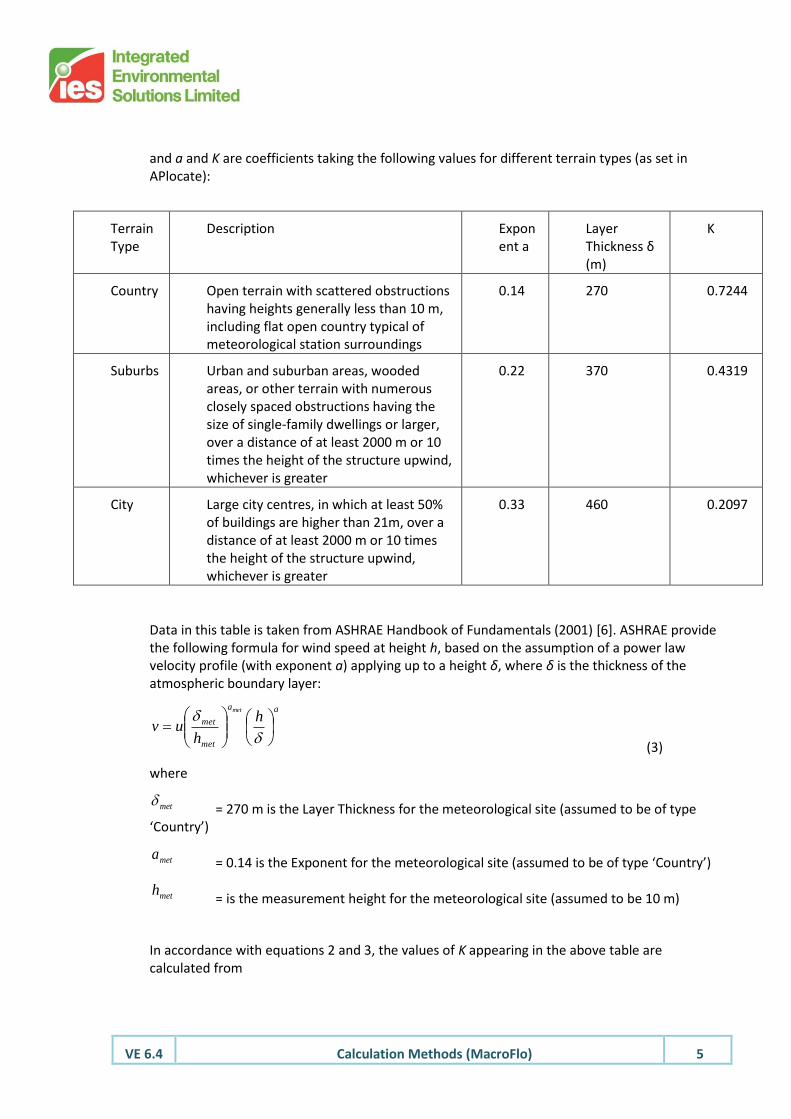
and a and K are coefficients taking the following values for different terrain types (as set in APlocate):

Terrain Type

Description Exponent a

Layer Thickness δ (m)

K

Country Open terrain with scattered obstructions having heights generally less than 10 m, including flat open country typical of meteorological station surroundings

0.14 270 0.7244

Suburbs Urban and suburban areas, wooded areas, or other terrain with numerous closely spaced obstructions having the size of single-family dwellings or larger, over a distance of at least 2000 m or 10 times the height of the structure upwind, whichever is greater

0.22 370 0.4319

City Large city centres, in which at least 50% of buildings are higher than 21m, over a distance of at least 2000 m or 10 times the height of the structure upwind, whichever is greater

0.33 460 0.2097

Data in this table is taken from ASHRAE Handbook of Fundamentals (2001) [6]. ASHRAE provide the following formula for wind speed at height h, based on the assumption of a power law velocity profile (with exponent a) applying up to a height δ, where δ is the thickness of the atmospheric boundary layer:

(3)

where

= 270 m is the Layer Thickness for the meteorological site (assumed to be of type ‘Country’)

= 0.14 is the Exponent for the meteorological site (assumed to be of type ‘Country’)

= is the measurement height for the meteorological site (assumed to be 10 m)

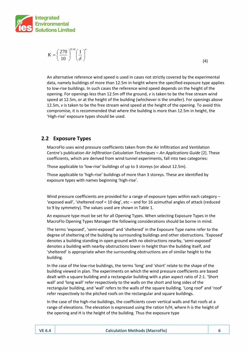
In accordance with equations 2 and 3, the values of K appearing in the above table are calculated from

aa

met

met h

huv

met

met

meta

meth


(4)

An alternative reference wind speed is used in cases not strictly covered by the experimental data, namely buildings of more than 12.5m in height where the specified exposure type applies to low-rise buildings. In such cases the reference wind speed depends on the height of the opening. For openings less than 12.5m off the ground, v is taken to be the free stream wind speed at 12.5m, or at the height of the building (whichever is the smaller). For openings above 12.5m, v is taken to be the free stream wind speed at the height of the opening. To avoid this compromise, it is recommended that where the building is more than 12.5m in height, the ‘High-rise’ exposure types should be used.

2.2 Exposure Types

MacroFlo uses wind pressure coefficients taken from the Air Infiltration and Ventilation Centre’s publication Air Infiltration Calculation Techniques – An Applications Guide [2]. These coefficients, which are derived from wind tunnel experiments, fall into two categories:

Those applicable to ‘low-rise’ buildings of up to 3 storeys (or about 12.5m).

Those applicable to ‘high-rise’ buildings of more than 3 storeys. These are identified by exposure types with names beginning ‘high-rise’.

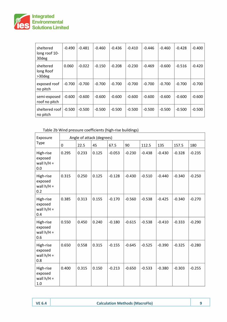
Wind pressure coefficients are provided for a range of exposure types within each category – ‘exposed wall’, ‘sheltered roof < 10 deg’, etc – and for 16 azimuthal angles of attack (reduced to 9 by symmetry). The values used are shown in Table 1.

An exposure type must be set for all Opening Types. When selecting Exposure Types in the MacroFlo Opening Types Manager the following considerations should be borne in mind.

The terms ‘exposed’, ‘semi-exposed’ and ‘sheltered’ in the Exposure Type name refer to the degree of sheltering of the building by surrounding buildings and other obstructions. ‘Exposed’ denotes a building standing in open ground with no obstructions nearby, ‘semi-exposed’ denotes a building with nearby obstructions lower in height than the building itself, and ‘sheltered’ is appropriate when the surrounding obstructions are of similar height to the building.

In the case of the low-rise buildings, the terms ‘long’ and ‘short’ relate to the shape of the building viewed in plan. The experiments on which the wind pressure coefficients are based dealt with a square building and a rectangular building with a plan aspect ratio of 2:1. ‘Short wall’ and ‘long wall’ refer respectively to the walls on the short and long sides of the rectangular building, and ‘wall’ refers to the walls of the square building. ‘Long roof’ and ‘roof’ refer respectively to the pitched roofs on the rectangular and square buildings.

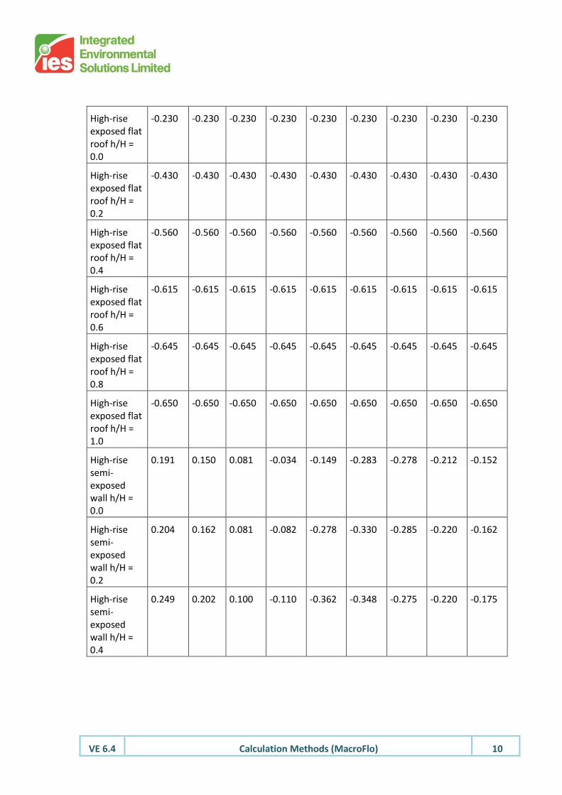
In the case of the high-rise buildings, the coefficients cover vertical walls and flat roofs at a range of elevations. The elevation is expressed using the ration h/H, where h is the height of the opening and H is the height of the building. Thus the exposure type

a

K

1

10

27014.0


high-rise semi-exp wall h/H=0.6

would be appropriate for an opening in a wall about 60% of the way up a building surrounded by other buildings of lesser height.

When selecting appropriate exposure types for MacroFlo Opening Types, you should make a judgement as to which of the available exposure types most accurately describes the exposure of the surfaces to which the Opening Types are to be assigned.

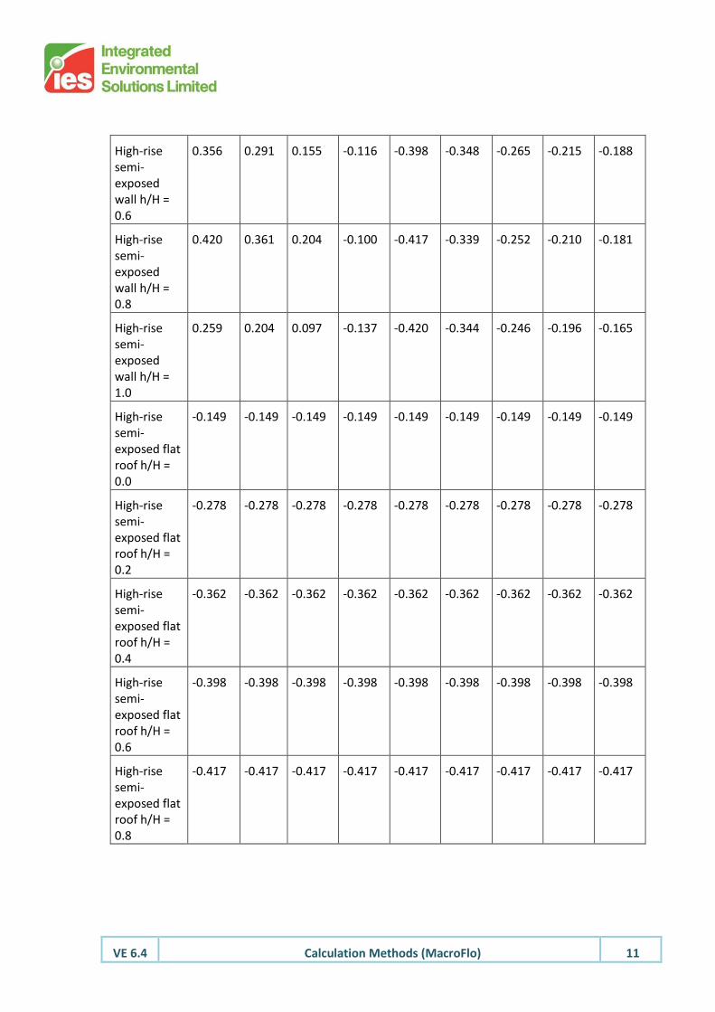
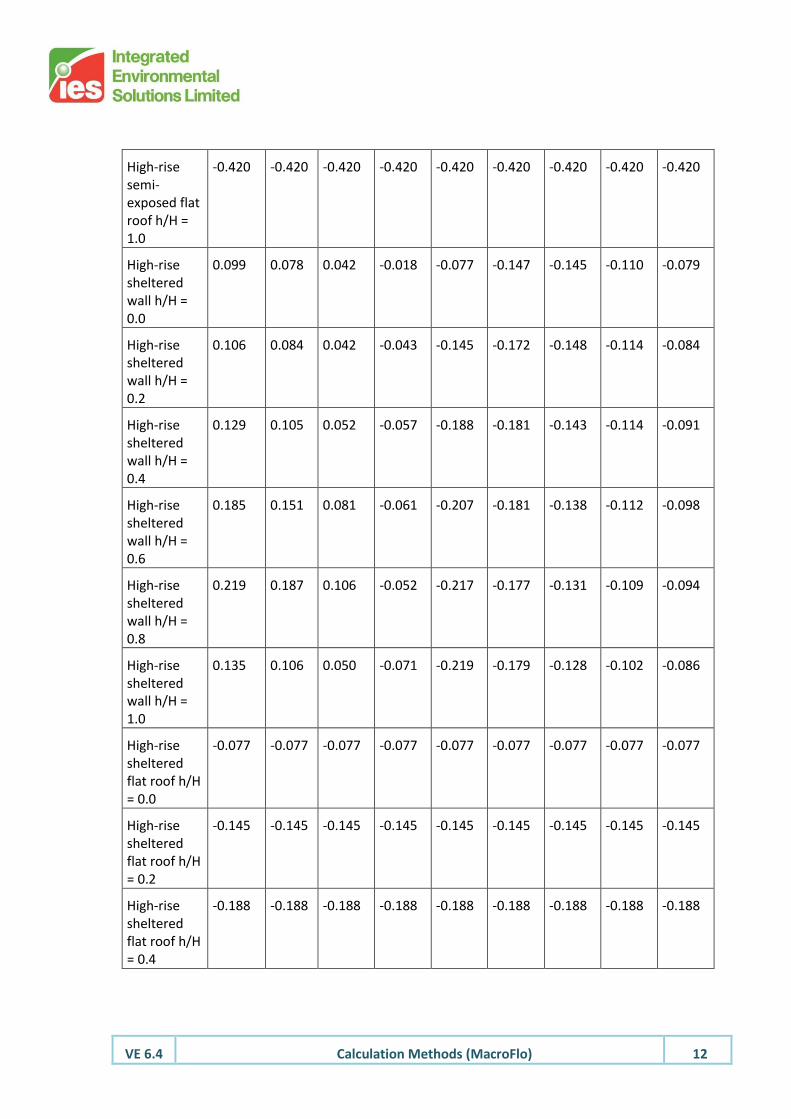
To cover flat roofs, which were not treated in the experimental study, additional Exposure Types have been added: ‘exposed flat roof’, ‘semi-exposed flat roof’, ‘sheltered flat roof’ and so on. Wind pressure coefficients for these Exposure Types have been estimated by extrapolating the available experimental data.

An exposure type appropriate for internal openings, ‘internal’, is also provided. If applied to external openings, this exposure type sets all wind pressure coefficients to zero, allowing you to investigate flow patterns in the absence of wind pressures.

2.3 Wind Turbulence

Adjustments are applied to wind pressures to allow for the effects of wind turbulence, as described in a later section.

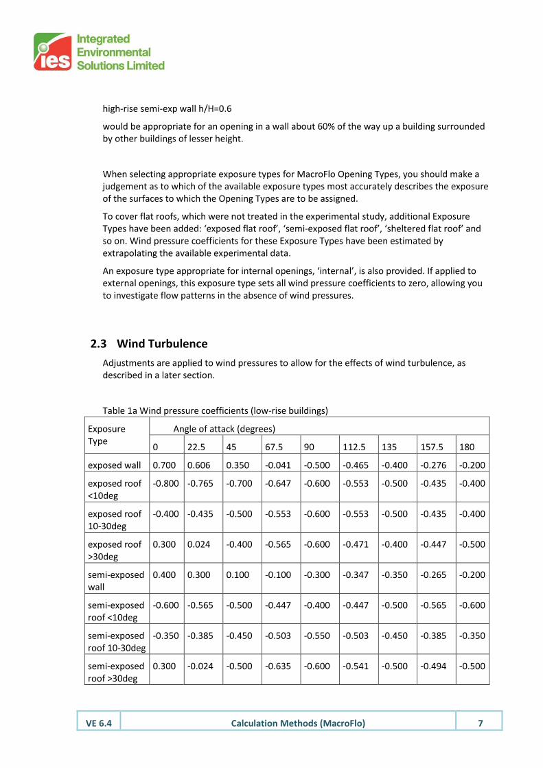
Table 1a Wind pressure coefficients (low-rise buildings)

Exposure Type

Angle of attack (degrees)

0 22.5 45 67.5 90 112.5 135 157.5 180

exposed wall 0.700 0.606 0.350 -0.041 -0.500 -0.465 -0.400 -0.276 -0.200

exposed roof <10deg

-0.800 -0.765 -0.700 -0.647 -0.600 -0.553 -0.500 -0.435 -0.400

exposed roof 10-30deg

-0.400 -0.435 -0.500 -0.553 -0.600 -0.553 -0.500 -0.435 -0.400

exposed roof >30deg

0.300 0.024 -0.400 -0.565 -0.600 -0.471 -0.400 -0.447 -0.500

semi-exposed wall

0.400 0.300 0.100 -0.100 -0.300 -0.347 -0.350 -0.265 -0.200

semi-exposed roof <10deg

-0.600 -0.565 -0.500 -0.447 -0.400 -0.447 -0.500 -0.565 -0.600

semi-exposed roof 10-30deg

-0.350 -0.385 -0.450 -0.503 -0.550 -0.503 -0.450 -0.385 -0.350

semi-exposed roof >30deg

0.300 -0.024 -0.500 -0.635 -0.600 -0.541 -0.500 -0.494 -0.500


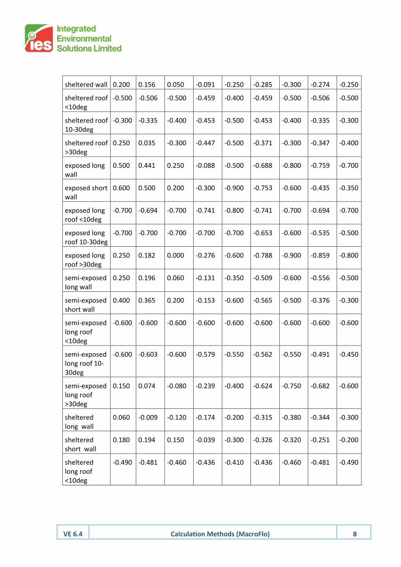
sheltered wall 0.200 0.156 0.050 -0.091 -0.250 -0.285 -0.300 -0.274 -0.250

sheltered roof <10deg

-0.500 -0.506 -0.500 -0.459 -0.400 -0.459 -0.500 -0.506 -0.500

sheltered roof 10-30deg

-0.300 -0.335 -0.400 -0.453 -0.500 -0.453 -0.400 -0.335 -0.300

sheltered roof >30deg

0.250 0.035 -0.300 -0.447 -0.500 -0.371 -0.300 -0.347 -0.400

exposed long wall

0.500 0.441 0.250 -0.088 -0.500 -0.688 -0.800 -0.759 -0.700

exposed short wall

0.600 0.500 0.200 -0.300 -0.900 -0.753 -0.600 -0.435 -0.350

exposed long roof <10deg

-0.700 -0.694 -0.700 -0.741 -0.800 -0.741 -0.700 -0.694 -0.700

exposed long roof 10-30deg

-0.700 -0.700 -0.700 -0.700 -0.700 -0.653 -0.600 -0.535 -0.500

exposed long roof >30deg

0.250 0.182 0.000 -0.276 -0.600 -0.788 -0.900 -0.859 -0.800

semi-exposed long wall

0.250 0.196 0.060 -0.131 -0.350 -0.509 -0.600 -0.556 -0.500

semi-exposed short wall

0.400 0.365 0.200 -0.153 -0.600 -0.565 -0.500 -0.376 -0.300

semi-exposed long roof <10deg

-0.600 -0.600 -0.600 -0.600 -0.600 -0.600 -0.600 -0.600 -0.600

semi-exposed long roof 10-30deg

-0.600 -0.603 -0.600 -0.579 -0.550 -0.562 -0.550 -0.491 -0.450

semi-exposed long roof >30deg

0.150 0.074 -0.080 -0.239 -0.400 -0.624 -0.750 -0.682 -0.600

sheltered long wall

0.060 -0.009 -0.120 -0.174 -0.200 -0.315 -0.380 -0.344 -0.300

sheltered short wall

0.180 0.194 0.150 -0.039 -0.300 -0.326 -0.320 -0.251 -0.200

sheltered long roof <10deg

-0.490 -0.481 -0.460 -0.436 -0.410 -0.436 -0.460 -0.481 -0.490


sheltered long roof 10-30deg

-0.490 -0.481 -0.460 -0.436 -0.410 -0.446 -0.460 -0.428 -0.400

sheltered long Roof >30deg

0.060 -0.022 -0.150 -0.208 -0.230 -0.469 -0.600 -0.516 -0.420

exposed roof no pitch

-0.700 -0.700 -0.700 -0.700 -0.700 -0.700 -0.700 -0.700 -0.700

semi-exposed roof no pitch

-0.600 -0.600 -0.600 -0.600 -0.600 -0.600 -0.600 -0.600 -0.600

sheltered roof no pitch

-0.500 -0.500 -0.500 -0.500 -0.500 -0.500 -0.500 -0.500 -0.500

Table 2b Wind pressure coefficients (high-rise buildings)

Exposure Type

Angle of attack (degrees)

0 22.5 45 67.5 90 112.5 135 157.5 180

High-rise exposed wall h/H = 0.0

0.295 0.233 0.125 -0.053 -0.230 -0.438 -0.430 -0.328 -0.235


0.315 0.250 0.125 -0.128 -0.430 -0.510 -0.440 -0.340 -0.250


0.385 0.313 0.155 -0.170 -0.560 -0.538 -0.425 -0.340 -0.270


0.550 0.450 0.240 -0.180 -0.615 -0.538 -0.410 -0.333 -0.290


0.650 0.558 0.315 -0.155 -0.645 -0.525 -0.390 -0.325 -0.280


0.400 0.315 0.150 -0.213 -0.650 -0.533 -0.380 -0.303 -0.255


High-rise exposed flat roof h/H = 0.0

-0.230 -0.230 -0.230 -0.230 -0.230 -0.230 -0.230 -0.230 -0.230


-0.430 -0.430 -0.430 -0.430 -0.430 -0.430 -0.430 -0.430 -0.430


-0.560 -0.560 -0.560 -0.560 -0.560 -0.560 -0.560 -0.560 -0.560


-0.615 -0.615 -0.615 -0.615 -0.615 -0.615 -0.615 -0.615 -0.615


-0.645 -0.645 -0.645 -0.645 -0.645 -0.645 -0.645 -0.645 -0.645


-0.650 -0.650 -0.650 -0.650 -0.650 -0.650 -0.650 -0.650 -0.650

High-rise semi-exposed wall h/H = 0.0

0.191 0.150 0.081 -0.034 -0.149 -0.283 -0.278 -0.212 -0.152


0.204 0.162 0.081 -0.082 -0.278 -0.330 -0.285 -0.220 -0.162


0.249 0.202 0.100 -0.110 -0.362 -0.348 -0.275 -0.220 -0.175



0.356 0.291 0.155 -0.116 -0.398 -0.348 -0.265 -0.215 -0.188


0.420 0.361 0.204 -0.100 -0.417 -0.339 -0.252 -0.210 -0.181


0.259 0.204 0.097 -0.137 -0.420 -0.344 -0.246 -0.196 -0.165

High-rise semi-exposed flat roof h/H = 0.0

-0.149 -0.149 -0.149 -0.149 -0.149 -0.149 -0.149 -0.149 -0.149


-0.278 -0.278 -0.278 -0.278 -0.278 -0.278 -0.278 -0.278 -0.278


-0.362 -0.362 -0.362 -0.362 -0.362 -0.362 -0.362 -0.362 -0.362


-0.398 -0.398 -0.398 -0.398 -0.398 -0.398 -0.398 -0.398 -0.398


-0.417 -0.417 -0.417 -0.417 -0.417 -0.417 -0.417 -0.417 -0.417



-0.420 -0.420 -0.420 -0.420 -0.420 -0.420 -0.420 -0.420 -0.420

High-rise sheltered wall h/H = 0.0

0.099 0.078 0.042 -0.018 -0.077 -0.147 -0.145 -0.110 -0.079


0.106 0.084 0.042 -0.043 -0.145 -0.172 -0.148 -0.114 -0.084


0.129 0.105 0.052 -0.057 -0.188 -0.181 -0.143 -0.114 -0.091


0.185 0.151 0.081 -0.061 -0.207 -0.181 -0.138 -0.112 -0.098


0.219 0.187 0.106 -0.052 -0.217 -0.177 -0.131 -0.109 -0.094


0.135 0.106 0.050 -0.071 -0.219 -0.179 -0.128 -0.102 -0.086

High-rise sheltered flat roof h/H = 0.0

-0.077 -0.077 -0.077 -0.077 -0.077 -0.077 -0.077 -0.077 -0.077


-0.145 -0.145 -0.145 -0.145 -0.145 -0.145 -0.145 -0.145 -0.145


-0.188 -0.188 -0.188 -0.188 -0.188 -0.188 -0.188 -0.188 -0.188



-0.207 -0.207 -0.207 -0.207 -0.207 -0.207 -0.207 -0.207 -0.207


-0.217 -0.217 -0.217 -0.217 -0.217 -0.217 -0.217 -0.217 -0.217


-0.219 -0.219 -0.219 -0.219 -0.219 -0.219 -0.219 -0.219 -0.219


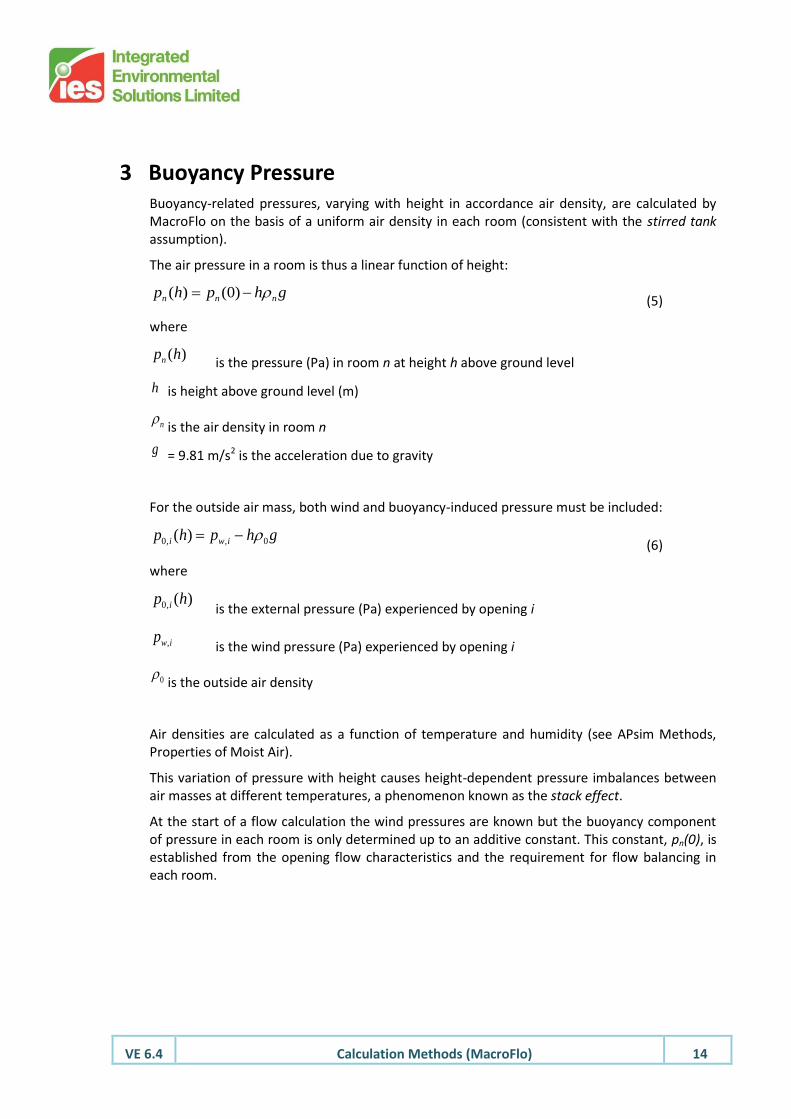
3 Buoyancy Pressure Buoyancy-related pressures, varying with height in accordance air density, are calculated by MacroFlo on the basis of a uniform air density in each room (consistent with the stirred tank assumption).

The air pressure in a room is thus a linear function of height:

(5)

where

is the pressure (Pa) in room n at height h above ground level

is height above ground level (m)

is the air density in room n

= 9.81 m/s2 is the acceleration due to gravity

For the outside air mass, both wind and buoyancy-induced pressure must be included:

(6)

where

is the external pressure (Pa) experienced by opening i

is the wind pressure (Pa) experienced by opening i

is the outside air density

Air densities are calculated as a function of temperature and humidity (see APsim Methods, Properties of Moist Air).

This variation of pressure with height causes height-dependent pressure imbalances between air masses at different temperatures, a phenomenon known as the stack effect.

At the start of a flow calculation the wind pressures are known but the buoyancy component of pressure in each room is only determined up to an additive constant. This constant, pn(0), is established from the opening flow characteristics and the requirement for flow balancing in each room.

ghphp nnn )0()(

)(hpn

h

n

g

ghphp iwi 0,,0 )(

)(,0 hp i

iwp ,

0


4 Flow Characteristics The flow through each opening is calculated as a function of imposed pressure difference and the characteristics of the opening. These characteristics differ for cracks and larger openings.

4.1 Flow Characteristics for Cracks

For a crack the dependence of flow on pressure difference is assumed to take the form

(7)

where

is the air flow through the crack (l/s)

is the Crack Flow Coefficient (l s-1 m-1 Pa-0.6)

is the length of the crack (m)

is the density of air entering the crack (kg/m3)

= 1.21 kg/m3 is a reference air density

is the pressure difference across the crack (Pa).

Equation 7 represents a best fit to a large range of experimental data analysed by the Air Infiltration and Ventilation Centre [1]. In this treatment the expression has been generalised on dimensional grounds by introducing a dependence on air density.

Representative measured values of the Crack Flow Coefficient for windows and doors are given in Table 3 and Table 4. These values are taken from [1].

Table 3 Crack Flow Coefficients (l s-1 m-1 Pa-0.6) – Windows

Lower Quartile

Median Upper Quartile

Windows (Weatherstripped)

Hinged

Sliding

0.086

0.079

0.13

0.15

0.41

0.21

Windows (Non-weatherstripped)

Hinged

Sliding

0.39

0.18

0.74

0.23

1.1

0.37

6.05.0)/( pCLq ref

q

C

L

ref

p


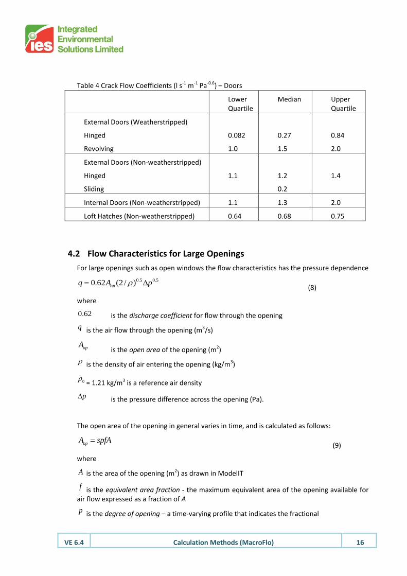
Table 4 Crack Flow Coefficients (l s-1 m-1 Pa-0.6) – Doors

Lower Quartile

Median Upper Quartile

External Doors (Weatherstripped)

Hinged

Revolving

0.082

1.0

0.27

1.5

0.84

2.0

External Doors (Non-weatherstripped)

Hinged

Sliding

1.1

1.2

0.2

1.4

Internal Doors (Non-weatherstripped) 1.1 1.3 2.0

Loft Hatches (Non-weatherstripped) 0.64 0.68 0.75

4.2 Flow Characteristics for Large Openings

For large openings such as open windows the flow characteristics has the pressure dependence

(8)

where

is the discharge coefficient for flow through the opening

is the air flow through the opening (m3/s)

is the open area of the opening (m2)

is the density of air entering the opening (kg/m3)

= 1.21 kg/m3 is a reference air density

is the pressure difference across the opening (Pa).

The open area of the opening in general varies in time, and is calculated as follows:

(9)

where

is the area of the opening (m2) as drawn in ModelIT

is the equivalent area fraction - the maximum equivalent area of the opening available for air flow expressed as a fraction of A

is the degree of opening – a time-varying profile that indicates the fractional

5.05.0)/2(62.0 pAq op

62.0

q

opA

0

p

spfAAop

A

f

p


extent to which the window is open at any given time (subject to the control signal s)

is a control signal relating to the (optional) control of window opening in response to room temperature

The variables p and s relate to the parameters Degree of Opening and Threshold Temperature set in the MacroFlo Opening Types Manager program.

Degree of Opening (% Profile) is a percentage profile allowing the degree of window or door opening to be specified as a function of time. Subject to the Temperature Threshold control, the area of the opening will be varied by modulating the Openable Area with the Degree of Opening percentage profile. When the Degree of Opening profile is zero, or when the Threshold Temperature control dictates that the window or door is closed, the opening will be treated as a crack.

Threshold Temperature (ºC) allows for window opening to be controlled on the basis of room temperature. Threshold Temperature is the temperature in the room adjacent to the opening which, when exceeded, will trigger the opening of the window or door. Once open, it will remain so (possibly in varying degrees) until the Degree of Opening percentage profile falls to zero, regardless of subsequent values of the adjacent room air temperature. A low value for Threshold Temperature (for example 0ºC) will ensure that the pattern of opening simply follows the Degree of Opening percentage profile.

The discharge coefficient (0.62) used in equation 8 is appropriate for openings that are small in relation to the adjacent spaces. Where this is not the case, adjustments to opening areas may be appropriate. See section 7 Techniques for Modelling Flow in Facades.

4.2.1 Equivalent Area Fraction

The equivalent area fraction is calculated depending on the category of opening selected and related variables input.

Users should be clear about the meaning of equivalent area as these terms are often loosely defined; a list of definitions is provided below and how they are applied in the <VE>:

The structural opening area: the area of the "hole in the wall" required to fit the window or louvre/grille. In the <VE> the user can draw a notional window (of which a sub-area(s) maybe openable) or individually draw each opening leaf. The user can use the MacroFlo Openable area % input to allow for non-openable portions or frame area on individual leafs etc.

s


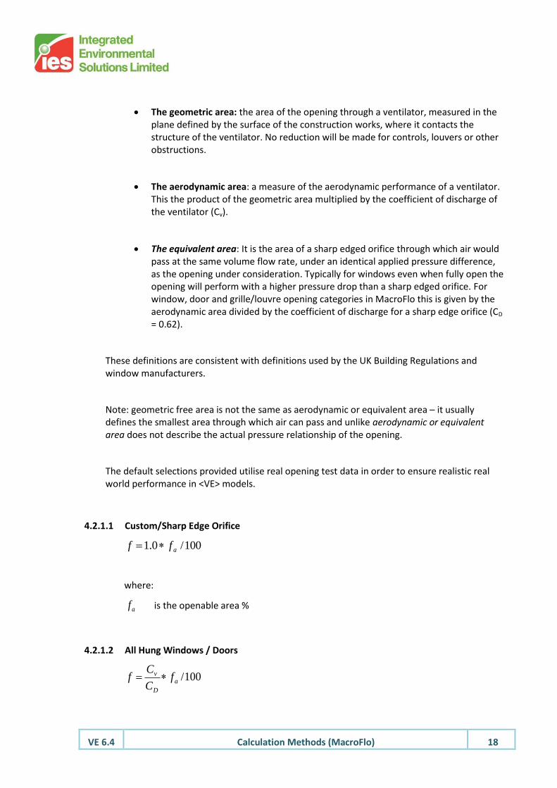
The geometric area: the area of the opening through a ventilator, measured in the plane defined by the surface of the construction works, where it contacts the structure of the ventilator. No reduction will be made for controls, louvers or other obstructions.

The aerodynamic area: a measure of the aerodynamic performance of a ventilator. This the product of the geometric area multiplied by the coefficient of discharge of the ventilator (Cv).

The equivalent area: It is the area of a sharp edged orifice through which air would pass at the same volume flow rate, under an identical applied pressure difference, as the opening under consideration. Typically for windows even when fully open the opening will perform with a higher pressure drop than a sharp edged orifice. For window, door and grille/louvre opening categories in MacroFlo this is given by the aerodynamic area divided by the coefficient of discharge for a sharp edge orifice (CD = 0.62).

These definitions are consistent with definitions used by the UK Building Regulations and window manufacturers.

Note: geometric free area is not the same as aerodynamic or equivalent area – it usually defines the smallest area through which air can pass and unlike aerodynamic or equivalent area does not describe the actual pressure relationship of the opening.

The default selections provided utilise real opening test data in order to ensure realistic real world performance in <VE> models.

4.2.1.1 Custom/Sharp Edge Orifice

100/0.1 aff

where:

af is the openable area %

4.2.1.2 All Hung Windows / Doors

100/a

D

v fC

Cf


where:

vC is a discharge coefficient interpolated from the table below.

CD is the discharge coefficient for a sharp edge orifice (0.62)



Window performance data has been collated from manufacturer’s test data.

vC Factors Calculations:

Side hung window / door: Proportions

L/H < 0.5 0.5 = L/H <1 1 = L/H <2

L/H > 2

Opening angle deg Cv Cv Cv Cv

10 0.1 0.17 0.24 0.34

20 0.22 0.31 0.39 0.51

30 0.36 0.43 0.5 0.6

45 0.5 0.54 0.64 0.65

60 0.58 0.6 0.63 0.67

90 0.64 0.65 0.65 0.67

Centre hung window: Proportions

L/H = 1 L/H > 2

Opening angle deg Cv Cv

15 0.15 0.13

30 0.30 0.27

45 0.44 0.39

60 0.56 0.56

90 0.64 0.61

Top hung window: Proportions

L/H < 0.5 0.5 = L/H <1 1 = L/H <2

L/H > 2


10 0.34 0.24 0.17 0.1

20 0.52 0.39 0.3 0.23

30 0.6 0.5 0.43 0.36

45 0.65 0.58 0.54 0.5

60 0.67 0.63 0.6 0.58

90 0.68 0.65 0.65 0.64


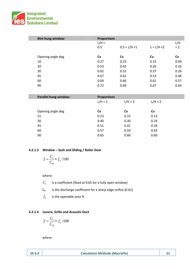
Btm hung window: Proportions

L/H < 0.5 0.5 = L/H <1 1 = L/H <2

L/H > 2


10 0.27 0.23 0.15 0.09

20 0.53 0.42 0.26 0.16

30 0.62 0.52 0.37 0.26

45 0.67 0.62 0.53 0.46

60 0.69 0.66 0.61 0.57

90 0.72 0.69 0.67 0.64

Parallel hung window: Proportions

L/H = 1 L/H = 2 L/H > 2

Opening angle deg Cv Cv Cv

15 0.23 0.15 0.13

30 0.40 0.30 0.24

45 0.51 0.41 0.34

60 0.57 0.50 0.43

90 0.65 0.60 0.60

4.2.1.3 Window – Sash and Sliding / Roller Door

100/a

D

v fC

Cf

where:

vC is a coefficient (fixed at 0.65 for a fully open window)



4.2.1.4 Louvre, Grille and Acoustic Duct

100/a

D

v fC

Cf

where:


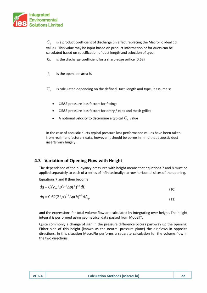
xC is a product coefficient of discharge (in effect replacing the MacroFlo ideal Cd

value). This value may be input based on product information or for ducts can be calculated based on specification of duct length and selection of type.



xC is calculated depending on the defined Duct Length and type, it assume s:

CIBSE pressure loss factors for fittings

CIBSE pressure loss factors for entry / exits and mesh grilles

A notional velocity to determine a typical xC value

In the case of acoustic ducts typical pressure loss performance values have been taken from real manufacturers data, however it should be borne in mind that acoustic duct inserts vary hugely.

4.3 Variation of Opening Flow with Height

The dependence of the buoyancy pressures with height means that equations 7 and 8 must be applied separately to each of a series of infinitesimally narrow horizontal slices of the opening.

Equations 7 and 8 then become

(10)

(11)

and the expressions for total volume flow are calculated by integrating over height. The height integral is performed using geometrical data passed from ModelIT.

Quite commonly a change of sign in the pressure difference occurs part-way up the opening. Either side of this height (known as the neutral pressure plane) the air flows in opposite directions. In this situation MacroFlo performs a separate calculation for the volume flow in the two directions.

dLhpCdq 6.05.0

0 )()/(

opdAhpdq 5.05.0 )()/2(62.0


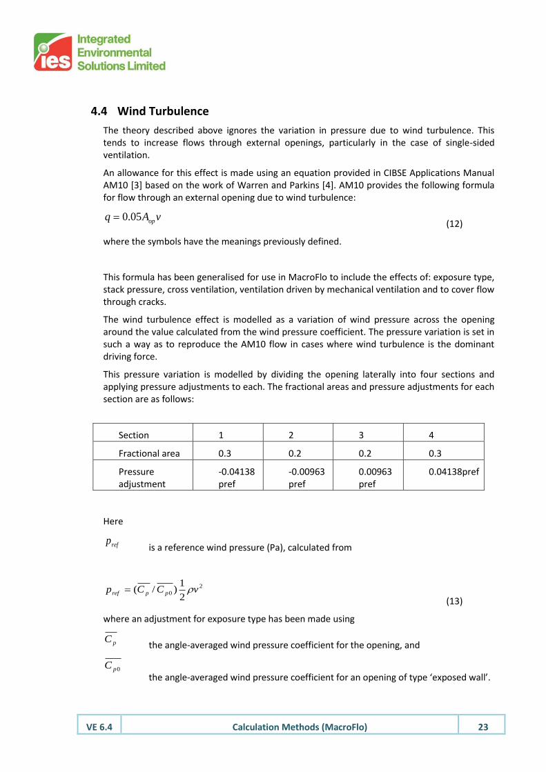
4.4 Wind Turbulence

The theory described above ignores the variation in pressure due to wind turbulence. This tends to increase flows through external openings, particularly in the case of single-sided ventilation.

An allowance for this effect is made using an equation provided in CIBSE Applications Manual AM10 [3] based on the work of Warren and Parkins [4]. AM10 provides the following formula for flow through an external opening due to wind turbulence:

(12)

where the symbols have the meanings previously defined.

This formula has been generalised for use in MacroFlo to include the effects of: exposure type, stack pressure, cross ventilation, ventilation driven by mechanical ventilation and to cover flow through cracks.

The wind turbulence effect is modelled as a variation of wind pressure across the opening around the value calculated from the wind pressure coefficient. The pressure variation is set in such a way as to reproduce the AM10 flow in cases where wind turbulence is the dominant driving force.

This pressure variation is modelled by dividing the opening laterally into four sections and applying pressure adjustments to each. The fractional areas and pressure adjustments for each section are as follows:

Section 1 2 3 4

Fractional area 0.3 0.2 0.2 0.3

Pressure adjustment

-0.04138 pref

-0.00963 pref

0.00963 pref

0.04138pref

Here

is a reference wind pressure (Pa), calculated from

(13)

where an adjustment for exposure type has been made using

the angle-averaged wind pressure coefficient for the opening, and

the angle-averaged wind pressure coefficient for an opening of type ‘exposed wall’.

vAq op05.0

refp

2

02

1)/( vCCp ppref

pC

0pC


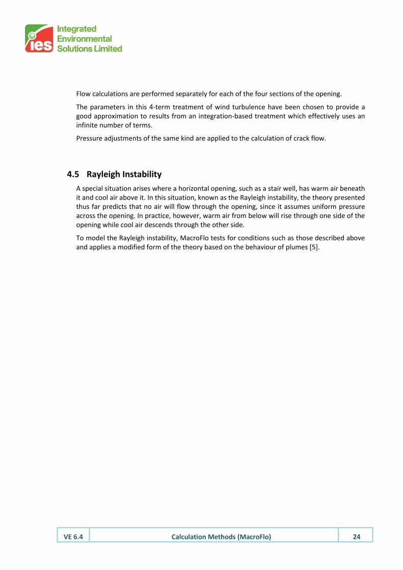
Flow calculations are performed separately for each of the four sections of the opening.

The parameters in this 4-term treatment of wind turbulence have been chosen to provide a good approximation to results from an integration-based treatment which effectively uses an infinite number of terms.

Pressure adjustments of the same kind are applied to the calculation of crack flow.

4.5 Rayleigh Instability

A special situation arises where a horizontal opening, such as a stair well, has warm air beneath it and cool air above it. In this situation, known as the Rayleigh instability, the theory presented thus far predicts that no air will flow through the opening, since it assumes uniform pressure across the opening. In practice, however, warm air from below will rise through one side of the opening while cool air descends through the other side.

To model the Rayleigh instability, MacroFlo tests for conditions such as those described above and applies a modified form of the theory based on the behaviour of plumes [5].


5 Building Air Flow Balance For a given set of room conditions (temperature and humidity) MacroFlo solves the air flow problem by balancing net air mass flows into and out of each room. The components of this air flow balance are:

Net air inflow for each of the room’s openings, calculated as described above.

Any net room airflow imbalance imposed by the system simulation program APhvac.

Within each room there is assumed to be no pressure variation except the density-related variation with height.

The network of flow and pressure relationships is solved by linearisation and iteration. The result of this calculation is a set of values for the room pressures extrapolated to the ground level datum, pn(0), together with flow rates in each direction through each opening. The criterion for convergence is that each room’s mass flows should balance to an accuracy of 0.0001 kg/s.


6 Building Air Flow, Heat and Moisture Balances MacroFlo exchanges data with APsim and APhvac dynamically to achieve the simultaneous solution of the inter-dependent thermal and air flow balances. In the course of an iterative procedure, room temperature and humidity conditions (together with any APhvac net supply or extract rates) are repeatedly passed to MacroFlo, which calculates the resulting natural ventilation flows. These flows are then used by APsim to update the room conditions, and so on. Upon convergence, this procedure balances both air flows and heat flows for each room.


7 Techniques for Modelling Flow in Façades and Flues The theory applied in MacroFlo is based on the flow characteristics of openings that are small in relation to the spaces they connect. Whilst this is a good approximation for most windows, doors and louvres, it is a poor approximation in some other modelling situations, notably flow in façade cavities and flues. For this type of situation, where the openings have a diameter similar or equal to the diameter of the adjacent spaces, adjustments to the opening parameters are necessary in order to achieve a good model.

In the case of flow in a façade cavity, there are three sources of flow resistance:

1. Resistance associated with the exchange of air between the cavity, the outside environment and the adjacent building spaces.

2. Resistance offered by obstructions in the cavity. These may take the form of constrictions, obstructions protruding from the sides, walkways etc.

3. Frictional resistance with the walls of the cavity.

These will now be dealt with in turn.

7.1 External Openings

On the whole, openings in this category are well represented by the standard theory and require no adjustment.

7.2 Constrictions in the Cavity

There is an extensive data available on the resistance to flow in ducts imposed by constrictions, expansions, contractions, grilles and other forms of obstruction. This data can be applied in MacroFlo in the following way.

A flow coefficient, k, is defined for the obstruction, as follows:

(14)

where

is the pressure difference across the obstruction

is the flow coefficient (sometimes referred to simply as ‘resistance’)

is the air density

is the mean air speed at a specified cross section of the flow

2

21 ukp

p

k

u


The point at which u is defined needs to be specified carefully. If u is defined for all obstructions at a common point in the flow (for example an unimpeded section of the duct), it is possible to combine k coefficients for a set of obstructions in series by simple addition.

If k is known for an obstruction or a set of obstructions it can be used to calculate a correction to the area of MacroFlo opening such that the opening will have the desired flow resistance.

Let us assume that k is defined in terms of the mean speed of air in the unimpeded duct, which has area Ad, and that the obstruction is to be represented by a MacroFlo opening of area Ao.

The pressure/flow relationship for the MacroFlo opening is

(15)

where

is the pressure difference across the opening

= (1/0.62)2 is the flow coefficient (sometimes referred to simply as

‘resistance’) for openings which are small compared to their adjacent spaces

is the mean air speed of the air flow through the opening

uo is linked to u by the flow conservation equation

(16)

from which, by equations 14 and 15,

(17)

If the value of Ao calculated from equation 17 is used in MacroFlo the opening will correctly represent the resistance of the obstruction.

The most common type of obstruction is an orifice plate or grille, which abruptly reduces the area available to the flow by a factor σ, where σ < 1. For this type of obstruction a good approximation to the flow coefficient (applied to u in the unimpeded duct) is

(18)

7.3 Wall Resistance

The resistance of a duct due to friction with its walls can be expressed in terms of a friction factor, f:

(19)

2

21

oo ukp

p

ok

ou

uAuA doo

)62.0/()/( 5.05.0 kAAkkA ddoo

225.0 /)]2/)1[(1( k

DfLk /


where

is the flow coefficient, as defined in the previous section

is the friction factor

is the length of the duct

is the hydraulic diameter of the duct

For a duct with one dimension much larger than the other, D is twice the width, w, so

(20)

The friction factor, f, depends on the speed of the flow (usually expressed in terms of Reynolds number) and the roughness of the duct’s sides. Values can be read off a Moody diagram.

For typical flow speeds in façade cavities (i.e. Reynolds numbers greater than about 50000 and roughness factors ε/D greater than about 0.01), a good approximation to f is given by

(21)

where

is the surface roughness factor, defined as the ratio of the typical heights of

surface features to the hydraulic diameter.

Combining equations 20 and 21 we obtain

(22)

In reality this frictional resistance is distributed evenly along the duct. In MacroFlo it must be aggregated into discrete openings. Floor slabs are convenient places to position such openings.

The value of k calculated from equation 22 may be substituted directly into equation 17, or may alternatively be combined with a flow coefficient representing the resistance of an obstruction at the floor slab level:

(23)

where

is the obstruction flow coefficient from equation 7 or similar

is the duct resistance flow coefficient from equation 11,

is the combined flow coefficient.

k

f

L

D

)2/( wfLk

2

10 ]7.3/)/[(log2/1 Df

D/

)]4.7/)/[(log8/(2

10 wwLk

ductobs kkk

obsk

ductk

k


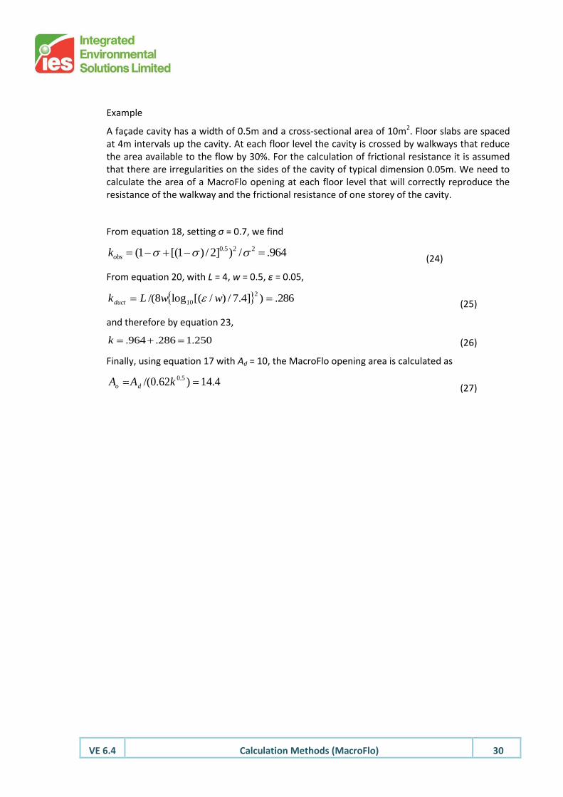
Example

A façade cavity has a width of 0.5m and a cross-sectional area of 10m2. Floor slabs are spaced at 4m intervals up the cavity. At each floor level the cavity is crossed by walkways that reduce the area available to the flow by 30%. For the calculation of frictional resistance it is assumed that there are irregularities on the sides of the cavity of typical dimension 0.05m. We need to calculate the area of a MacroFlo opening at each floor level that will correctly reproduce the resistance of the walkway and the frictional resistance of one storey of the cavity.

From equation 18, setting σ = 0.7, we find

(24)

From equation 20, with L = 4, w = 0.5, ε = 0.05,

(25)

and therefore by equation 23,

(26)

Finally, using equation 17 with Ad = 10, the MacroFlo opening area is calculated as

(27)

964./)]2/)1[(1( 225.0 obsk

286.)]4.7/)/[(log8/(2

10 wwLkduct

250.1286.964. k

4.14)62.0/( 5.0 kAA do


8 References 1. An Analysis and Data Summary of the AIVC’s Numerical Database. Technical Note AIVC

44, March 1994. Air Infiltration and Ventilation Centre.

2. Air Infiltration Calculation Techniques – An Applications Guide, Air Infiltration and Ventilation Centre. University of Warwick Science Park. Sovereign Court, Sir William Lyons Road, Coventry CV4 7EZ.

3. Applications Manual AM10: 1997. Natural ventilation in non-domestic buildings. CIBSE 1997.

4. Warren P R and Parkins L M. Window opening behaviour in office buildings Building Serv. Eng. Res.Technol. 5(3) pp 89-101 (1984).

5. L.C. Burmeister. Convective Heat Transfer. 2nd Edition. John Wiley & Sons, Inc. 1993.

6. ASHRAE Handbook of Fundamentals (2001).

macroflo calculation methods - iesve

Documents