making sense of africa's infrastructure endowment: a benchmark approach
TRANSCRIPT

WORKING PAPER 1
Making Sense of Africa’s Infrastructure Endowment: A Benchmarking Approach
Tito Yepes, Justin Pierce, and Vivien Foster
JANUARY 2008

© 2009 The International Bank for Reconstruction and Development / The World Bank
1818 H Street, NW
Washington, DC 20433 USA
Telephone: 202-473-1000
Internet: www.worldbank.org
E-mail: [email protected]
All rights reserved
A publication of the World Bank.
The World Bank
1818 H Sreet, NW
Washington, DC 20433 USA
The findings, interpretations, and conclusions expressed herein are those of the author(s) and do not necessarily reflect the views of the
Executive Directors of the International Bank for Reconstruction and Development / The World Bank or the governments they represent.
The World Bank does not guarantee the accuracy of the data included in this work. The boundaries, colors, denominations, and other
information shown on any map in this work do not imply any judgment on the part of The World Bank concerning the legal status of any territory or the endorsement or acceptance of such boundaries.
Rights and permissions
The material in this publication is copyrighted. Copying and/or transmitting portions or all of this work without permission may be a violation of applicable law. The International Bank for Reconstruction and Development / The World Bank encourages dissemination of its work and will normally grant permission to reproduce portions of the work promptly.
For permission to photocopy or reprint any part of this work, please send a request with complete information to the Copyright Clearance
Center Inc., 222 Rosewood Drive, Danvers, MA 01923 USA; telephone: 978-750-8400; fax: 978-750-4470; Internet: www.copyright.com.
All other queries on rights and licenses, including subsidiary rights, should be addressed to the Office of the Publisher, The World Bank, 1818 H Street, NW, Washington, DC 20433 USA; fax: 202-522-2422; e-mail: [email protected].

About AICD
This study is a product of the Africa Infrastructure Country
Diagnostic (AICD), a project designed to expand the
world’s knowledge of physical infrastructure in Africa.
AICD will provide a baseline against which future
improvements in infrastructure services can be measured,
making it possible to monitor the results achieved from
donor support. It should also provide a better empirical
foundation for prioritizing investments and designing
policy reforms in Africa’s infrastructure sectors.
AICD is based on an unprecedented effort to collect
detailed economic and technical data on African
infrastructure. The project has produced a series of reports
(such as this one) on public expenditure, spending needs,
and sector performance in each of the main infrastructure
sectors—energy, information and communication
technologies, irrigation, transport, and water and sanitation.
Africa’s Infrastructure—A Time for Transformation,
published by the World Bank in November 2009,
synthesizes the most significant findings of those reports.
AICD was commissioned by the Infrastructure Consortium
for Africa after the 2005 G-8 summit at Gleneagles, which
recognized the importance of scaling up donor finance for
infrastructure in support of Africa’s development.
The first phase of AICD focused on 24 countries that
together account for 85 percent of the gross domestic
product, population, and infrastructure aid flows of Sub-
Saharan Africa. The countries are: Benin, Burkina Faso,
Cape Verde, Cameroon, Chad, Côte d'Ivoire, the
Democratic Republic of Congo, Ethiopia, Ghana, Kenya,
Lesotho, Madagascar, Malawi, Mozambique, Namibia,
Niger, Nigeria, Rwanda, Senegal, South Africa, Sudan,
Tanzania, Uganda, and Zambia. Under a second phase of
the project, coverage is expanding to include as many other
African countries as possible.
Consistent with the genesis of the project, the main focus is
on the 48 countries south of the Sahara that face the most
severe infrastructure challenges. Some components of the
study also cover North African countries so as to provide a
broader point of reference. Unless otherwise stated,
therefore, the term “Africa” will be used throughout this
report as a shorthand for “Sub-Saharan Africa.”
The World Bank is implementing AICD with the guidance
of a steering committee that represents the African Union,
the New Partnership for Africa’s Development (NEPAD),
Africa’s regional economic communities, the African
Development Bank, the Development Bank of Southern
Africa, and major infrastructure donors.
Financing for AICD is provided by a multidonor trust fund
to which the main contributors are the U.K.’s Department
for International Development, the Public Private
Infrastructure Advisory Facility, Agence Française de
Développement, the European Commission, and Germany’s
KfW Entwicklungsbank. The Sub-Saharan Africa Transport
Policy Program and the Water and Sanitation Program
provided technical support on data collection and analysis
pertaining to their respective sectors. A group of
distinguished peer reviewers from policy-making and
academic circles in Africa and beyond reviewed all of the
major outputs of the study to ensure the technical quality of
the work.
The data underlying AICD’s reports, as well as the reports
themselves, are available to the public through an
interactive Web site, www.infrastructureafrica.org, that
allows users to download customized data reports and
perform various simulations. Inquiries concerning the
availability of data sets should be directed to the editors at
the World Bank in Washington, DC.
iii
Contents
Abstract iv
1 Methodological framework 1
2 The impact of environmental factors on infrastructure endowments 5
3 The impact of historical trends on infrastructure endowments 16
4 Conclusions 27
5 References 28
Annex A Alternative regression models 30
Annex B Country-specific deviations from regression models 31
Annex C Regional infrastructure endowment 35
About the authors
Tito Yepes is an economist in the World Bank’s Latin America and Caribbean Region. Justin Pierce is a doctoral student in economics at Georgetown University. Vivien Foster is a lead economist in the World Bank’s Africa Region. The authors thank Cesar Calderón for generously providing some of the data used in our analysis of the interplay of infrastructure and growth.

iv
Abstract
The objective of this paper is to explain the factors underlying Africa’s weak infrastructure
endowment and to identify suitable infrastructure goals for the region based on benchmarking
against international peers. The exercise is based on a dataset covering the stocks of key
infrastructure—including information and communication technology (ICT), power, roads, and
water—across 155 developing countries over the period 1960 to 2005. The paper also examines
subregional differences within Africa. We make use of regression techniques to control for a
comprehensive set of economic, demographic, geographic, and historic conditioning factors, as
well as adjusting for potential endogeneities.
Results show that Africa lags behind all other regions of the developing world in its
infrastructure endowment, except in ICT. By far the largest gaps arise in the power sector, with
generating capacity and household access to electricity in Africa at around half the levels
observed in South Asia. While it is often assumed that Africa’s infrastructure deficit is largely a
reflection of its relatively low income levels, this does not present a complete picture. Even
controlling for income group, we find that African countries have much more limited
infrastructure than income peers in other parts of the developing world. The reason appears to be
that Africa is a relatively difficult environment in which to develop infrastructure. Hence
countries that face the most challenging environment, in terms of low population density, weak
governance, and a history of conflict, present the poorest infrastructure endowments. However,
some environmental factors are more important than others. When all explanatory factors are
considered simultaneously, demographic variables (notably urbanization) appear to have the most
substantial effect on infrastructure endowments.
The overall regional picture masks significant geographic variations in infrastructure
endowments from country to country. We compared subregional endowments using four country
groupings: the Southern Africa Development Community; the East African Community, the
Economic Community of West African States, and Central Africa. Except with regard to various
road density measures, every African subregion underperformed relative to its expected value in
every infrastructure sector. SADC was the top performer with an infrastructure endowment more
comparable to East Asia than to the rest of Africa. EAC the worst performer on nearly all
dimensions of infrastructure, with Central Africa and ECOWAS somewhere in between. Oil-
exporting countries scored systematically and substantially worse than oil-importing countries,
suggesting that oil revenues are not being channeled into infrastructure investments.
Africa’s position relative to other developing regions has deteriorated over time. At the outset
of the data series, Africa was doing significantly better than other developing regions with
regards to overall road density, generation capacity, and fixed-line telephones, but growth rates in
these categories have been slower than in other regions. The most dramatic loss of ground has
come in electrical generating capacity, which has largely stagnated since 1980. The explanation
for this once again seems to lie in difficult environmental factors, in particular, low rates of
urbanization, that complicate the development of infrastructure.

he international community has recently committed itself to scaling up development
assistance to Africa, in part to address the continent’s major infrastructure deficit. But given
its income and other constraints, what level of infrastructure should Africa aim for? A related
issue is how well African institutions currently perform in sustaining and expanding infrastructure
stocks based on the resources that they have at their disposal. Both questions are amenable to
analysis through cross-country benchmarking of infrastructure stocks.
The objective of this paper is to shed light on Africa’s current infrastructure endowment and
clarify its future infrastructure goals. We pursue that objective by benchmarking the region’s
stock of key infrastructure—including information and communication technology (ICT), power,
roads, and water—against a dataset comprising 155 countries over the period 1960 to 2005. The
paper also sheds light on subregional differences, by comparing infrastructure stocks between
southern, central, eastern, and western Africa. In addition to pinpointing the factors that have
contributed to low infrastructure development on the continent, the benchmarking models serve
to identify suitable infrastructure targets that take into account the environmental difficulties that
countries face.
The paper is divided into three main sections. Section 1 lays down the methodological
framework used in the paper and relates it to the academic literature. Section 2 undertakes a
cross-sectional analysis that identifies the extent to which differences in infrastructure stocks
across countries can be explained in terms of differences in the geographical, demographic, and
economic environment that they face. Section 3 presents a panel data analysis that incorporates
the evolution of infrastructure stocks over time and thus clarifies the role of historical factors in
determining today’s infrastructure endowments.
1 Methodological framework
Benchmarking is a technique widely used in the management and regulatory fields to
compare the performance of firms against relevant peer groups. The benchmarking technique
employed in this paper was first proposed by Shleifer (1985), as a means of regulating so-called
“natural monopolies.” Shleifer argued that regulators should select socially optimal prices for
markets served by natural monopolies based on cost data from “similar” firms. Our approach also
resembles that used by Battese and Coelli (1993) to determine levels of “technical inefficiency”
among firms in a particular industry. Battese and Coelli estimated industry-level production
functions based on firm-level data and defined the distance between a firm’s actual and predicted
levels of production as its “technical inefficiency.” More recently, the World Bank’s annual
Doing Business report has illustrated the application of benchmarking techniques at the country
level. By creating a global database of investment climate indicators and conducting cross-
country comparisons, Doing Business has prompted a global debate about how to reduce red tape
and motivated policy makers to improve their competitiveness. A similar approach has been
applied to the infrastructure sectors in recent World Bank work at the country level (World Bank,
2004, 2005a, 2005b). Research in this area has benefited greatly from the availability of an
international panel of data on infrastructure stocks provided in Estache and Goicoechea (2005).
T

MAKING SENSE OF AFRICA’S INFRASTRUCTURE ENDOWMENT: A BENCHMARKING APPROACH
2
Here we perform a country-level benchmarking exercise for infrastructure stocks in Sub-
Saharan Africa, comparing them with a global peer group of developing countries. The paper
extends and deepens the work of Bogetic (2006) for the countries of the Southern African
Development Community (SADC), in particular by using regression techniques to control for a
wide range of differences in the operating environment faced by particular countries. In this way,
the benchmark against which each country is compared is individually adjusted to control for a
comprehensive set of economic, demographic, geographic, and historic conditioning factors.
The analysis is based on a panel dataset of all developing countries for the years 1960 to
2004. Developing countries are defined to be those in the low-income, lower-middle-income, and
upper-middle-income categories as defined by the World Bank. Data availability varies over the
period according to the specific infrastructure variable under consideration. Thus, road data are
available from 1960, ICT data from 1970, and electricity generation capacity data from 1980. In
the case of water and sanitation, only two time periods are available (1990 and 2002), while for
access to electricity no consistent time series could be found. The data are drawn from a variety
of global sources, including the World Bank’s World Development Indicators, the International
Telecommunications Union, and the World Economic Forum’s Global Competitiveness Report,
among others.
Our study contributes to the international benchmarking literature in three ways. In terms of
scope, it is the first study to benchmark the entire region of Sub-Saharan Africa, with an emphasis
on comparing regions of the developing world as well as the diverse subregions of Africa. It is
also the first study to base its predicted infrastructure levels on a panel dataset and to control for
potential endogeneity of regressors.
The benchmarking exercise compares each country’s actual infrastructure endowments to an
expected, or predicted, value based on its socioeconomic structure. The predicted values are
derived from an econometric model that explains variation in infrastructure levels among
developing countries based on a set of economic, demographic, and structural variables. This
exercise produces a measure of infrastructure endowment that controls for differences in all of the
socioeconomic variables included in the model. Thus, for example, it would be incorrect to
explain a lower-than-predicted infrastructure endowment for a particular country in terms of the
country’s low income, because the model includes income as an independent variable. Hence the
result already controls for differences in income. Note that here the concept of an expected, or
predicted, infrastructure level does not refer to any concept of demand, since actual levels of
infrastructure may also be driven by supply factors. Moreover, the expected value should not be
treated as an ideal; it simply expresses the average endowment of countries with comparable
characteristics.
Each country’s infrastructure endowment is measured by the deviation between its actual
endowment and the endowment predicted by the model (equation 1). A positive deviation
indicates that the country outperforms the benchmark provided by the econometric model (i.e.,
the average for the relevant peer group) and vice versa. The larger the absolute size of the
deviation, the greater the extent of the corresponding over- or underachievement.
MAKING SENSE OF AFRICA’S INFRASTRUCTURE ENDOWMENT: A BENCHMARKING APPROACH
3
(1) iiii predictedpredictedactualdeviation /)(=
Separate econometric models are estimated for nine different infrastructure variables—ICT
(fixed and mobile telephone lines, Internet connections), power (generating capacity and access to
electricity), roads (total and paved), water, and sanitation. All variables are normalized to
facilitate comparisons across countries. Roads are measured in terms of their density across the
country’s surface area. However, to allow for the fact that some countries include large areas of
uninhabitable wilderness, the total land area and total arable area are used as alternative means of
normalization. Generation capacity is normalized per million inhabitants; ICT variables are
normalized per thousand inhabitants. Electricity, water, and sanitation are expressed as
percentage household access rates. Access to water and sanitation correspond to the definitions of
improved water and sanitation specified in the Millennium Development Goals (United Nations
2007).
Our data reflect only the quantity of infrastructure; they say nothing of the quality and hence
economic value of those stocks. For example, two countries may have the same paved road
density, but one network may be well maintained and the other nearly impassable. Unfortunately,
there is no global dataset available that documents the quality of infrastructure stocks, although
some research does indicate a close correspondence between quality and quantity of infrastructure
(Calderon and Serven 2004). [
The first step is to estimate a simple, cross-sectional, ordinary least squares (OLS) model,
based on the most recent year of data available for each of the nine forms of infrastructure . This
is done following the specification given in equation (2), where y is an infrastructure stock, X is a
vector of independent variables (including economic, demographic, and environmental variables
as discussed below), and is an error term.
(2) iii Xy ++= '
Our approach extends the work of Canning (1998) to include a much wider set of explanatory
variables. In his seminal paper, Canning found that a significant portion of cross-country
variation in infrastructure endowments could be explained by economic and demographic
variables, such as per capita income, population density, urbanization rate, and growth of urban
population. To Canning’s set of regressors we add several demographic, public sector, and
structural variables. Ethnic fractionalization is also included as a regressor, since competition
between ethnic groups may affect infrastructure building programs. Similarly, a governance term
based on Transparency International’s Corruption Perceptions Index accounts for the impact of
wasteful or corrupt government management of infrastructure projects. A per capita measure of
foreign aid designated for infrastructure controls for significant variations in aid activity between
countries. Lastly, structural variables such as the share of manufacturing, agriculture, and exports
in GDP are incorporated, since the structure of the economy may affect demand for specific
infrastructure services. Our choice of explanatory variables draws upon an extensive exploratory
data analysis presented in the next section of the paper.

MAKING SENSE OF AFRICA’S INFRASTRUCTURE ENDOWMENT: A BENCHMARKING APPROACH
4
Several important limitations of this approach call for the use of panel data models. The
simple OLS cross-section is of some interest in that it replicates the results of earlier literature
(Canning 1998) and serves to isolate the effect of specific environmental variables that can be
identified as relevant from the exploratory data analysis. Nevertheless, it is subject to important
methodological limitations. First, the environmental variables only imperfectly control for the
myriad differences that arise in different country situations, which can be fully reflected only by
means of country-specific factors. Second, the long lag times in the development of infrastructure
stocks mean that historic trends play an important role in explaining a country’s current
infrastructure endowment. Third, the potential reverse causality from per capita income to
infrastructure stocks raises the possibility of endogeneity. All of these issues can be addressed
using panel data models that analyze a repeated cross-section for the same countries across a
number of years.
Our second step is therefore to estimate an OLS panel model that controls for country
differences (fixed effects) that affect the ease or difficulty of providing infrastructure services.
This is represented by equation (3), where yit is defined as the infrastructure level for country i at
time t, Xit is a matrix of socioeconomic and structural explanatory variables, and i is a time-
invariant country-specific fixed effect.
(3) itiitit Xy +++= '
Because the OLS fixed-effects model does not correct for the potential endogeneity of the
explanatory variables, our third step is to control for potential endogeneity of relevant regressors
using instrumental variables. It seems likely that per capita gross domestic product (GDP) will be
endogenous in the specification given in (3). In fact, there is already a large literature based on
the concept that causation lies in the opposite direction—that is, that expansion of infrastructure
services increases income and income growth. This direction of causality has been examined
extensively in Easterly and Serven (2003) and Calderon and Serven (2003, 2004). We draw on
this literature to choose appropriate instruments for per capita GDP. Specifically, we employ
some of the standard growth regressors from Calderon and Serven (2004), including trade
openness (trade as share of GDP), inflation, political risk index, government involvement in
economy (government consumption as share of GDP), domestic credit available to the private
sector (as share of GDP), and the terms of trade index. Adding these regressors gives us the
following equation:
(4) itititit Xy ++++= '
Xit contains the same set of regressors included in the cross-sectional OLS study. Per capita
GDP is instrumented using the standard growth variables described above. Lastly, it is important
to note that any time-invariant variables from the OLS regressions are dropped once country fixed
effects are included, which accounts for the smaller sets of coefficients reported for panel data
models later in the paper.1
1 The regressors used in (4) were also considered in a dynamic panel specification, using the technique
developed by Blundell and Bond (1998). These results are reported in Annex A.1 for comparison purposes,
MAKING SENSE OF AFRICA’S INFRASTRUCTURE ENDOWMENT: A BENCHMARKING APPROACH
5
2 The impact of environmental factors on
infrastructure endowments
Here we examine cross-country variations in today’s infrastructure stocks in the context of
the very different operating environments that countries face. We begin with a simple
benchmarking of infrastructure stocks by regions, subregions, income groups, and other
subcategories. We then use a cross-sectional OLS model to isolate the impact of individual
factors on infrastructure stocks in a multivariate framework. All averages presented are simple
unweighted averages across countries, as opposed to population-weighted averages for the
different country groupings. As a result, regional summary statistics may appear to differ from
commonly reported regional averages, which typically are based on a population weighting of
countries.
Variations across regions
Africa lags behind all other regions of the developing world in its infrastructure endowment,
except in ICT (table 2.1). This finding holds across a wide range of indicators including the
density of roads and paved roads, per capita capacity to generate electricity, and household access
to electricity, water, and sanitation. By far the largest gaps arise in the power sector, with
generating capacity and household access to electricity in Africa at around half the levels
observed in South Asia, and about a third of the levels observed in East Asia. The conclusion on
paved road density differs depending on whether one is considering total land area (in which case
Africa comes in last) or only arable area (in which case Africa comes in ahead of South Asia and
East Asia). In ICT, Africa significantly outperforms South Asia in density of mobile telephones
and Internet connections and comes close in terms of fixed-line density.
but they should be treated with caution because the slow adjustment process for infrastructure stocks may
overstate the significance of the lagged dependent variable.

MAKING SENSE OF AFRICA’S INFRASTRUCTURE ENDOWMENT: A BENCHMARKING APPROACH
6
Table 2.1 Infrastructure endowments by world region
Sector and measure
Su
b-
Sa
ha
ran
A
fric
a
So
uth
Asia
Ea
st
Asia
a
nd
Pa
cific
Eu
rop
e a
nd
C
en
tra
l A
sia
La
tin
A
me
rica
an
d
Ca
rib
be
an
Mid
dle
Ea
st
an
d N
ort
h
Afr
ica
Transport
Density of paved road network (km/1,000 km
2, 2001)
49 149 59 335 418 482
Density of paved road network (km/1,000 arable km
2, 2001)
1,087 675 588 1,208 4,826 6,890
Density of total road network (km/1,000 km
2, 2001)
152 306 237 576 740 599
Density of total road network (km/1,000 arable km
2, 2001)
2,558 1,400 5,385 2,160 8,850 30,319
Information and communication technology
Density of fixed-line telephones (subscribers per 1,000 people, 2004)
33 39 90 261 197 100
Density of mobile telephones (subscribers per 1,000 people, 2004)
101 86 208 489 350 224
Density of Internet connections (subscribers per 100 people, 2004)
2.8 1.7 6.6 16.4 14.1 10.1
Energy
Electrical generating capacity (MW per 1 million people, 2003)
70 154 231 970 464 496
Access to electricity (% of households with access, 2004)
18 44 57 — 79 88
Water and sanitation
Water (% of households with access, 2002)
63 72 75 87 90 85
Sanitation (% of households with access, 2002)
35 48 60 78 77 77
Sources: For transport, Easterly & Serven (2003); for ICT, International Telecommunications Union; for energy, Energy Information Agency, U.S. Department of Energy); for water and sanitation, World Development Indicators.
Africa’s deficit remains even when the countries of the region are compared with others in
the same income bracket (table 2.2). It is often assumed that Africa’s infrastructure deficit is
largely a reflection of its relatively low income levels. But the comparison with other developing
countries in the same income bracket shows that income does not tell the whole story. Africa’s
low-income countries (LICs) lag substantially behind those in other regions, while the same is
true for lower-middle-income countries (LMCs) and upper-middle-income countries (UMC). The
divergence is particularly striking for power and paved roads. Electrical generating capacity and
access to electricity in Africa are less than a third of the levels found in other UMCs around the
world.

MAKING SENSE OF AFRICA’S INFRASTRUCTURE ENDOWMENT: A BENCHMARKING APPROACH
7
Table 2.2 Infrastructure endowments by income group, Sub-Saharan Africa vs. other world regions
Country group
Low-income Lower-middle-income Upper-middle-income
Africa Other Ratio Africa Other Ratio Africa Other Ratio
Sector and measure (A) (B) (C=B/
A) (D) (E) (F=E/
D) (G) (H) (I=H/G)
Transport
Density of paved road network (km/1,000 km
2, 2001)
31 134 4.3 94 141 1.5 238 781 3.3
Density of paved road network (km/1,000 arable km
2, 2001)
290 728 2.5 1,176 1,919 1.6 11,086 7,415 0.7
Density of total road network (km/1,000 km
2, 2001)
137 211 1.5 215 343 1.6 293 1,171 4.0
Density of total road network (km/1,000 arable km
2, 2001)
1,535 2,194 1.4 4,233 10,624 2.5 14,179 13,375 0.9
Information and communication technology
Density of fixed-line telephones (subscribers per 1,000 people, 2004)
10 78 7.7 106 131 1.2 120 274 2.3
Density of mobile telephones (subscribers per 1,000 people, 2004)
55 86 1.6 201 298 1.5 422 554 1.3
Density of Internet connections (subscribers per 100 people, 2004)
2.0 3.2 1.6 5.1 8.0 1.6 10.3 26.2 2.5
Energy
Electrical generating capacity (MW per 1 million people, 2003)
37 326 8.8 256 434 1.7 246 861 3.5
Access to electricity (% of households with access, 2004)
16 41 2.6 35 80 2.3 28 95 3.4
Water and sanitation
Water (% of households with access, 2002)
60 72 1.2 75 86 1.2 90 93 1.0
Sanitation (% of households with access, 2002)
34 51 1.5 48 74 1.5 39 90 2.3
Sources: As for table 2.1.
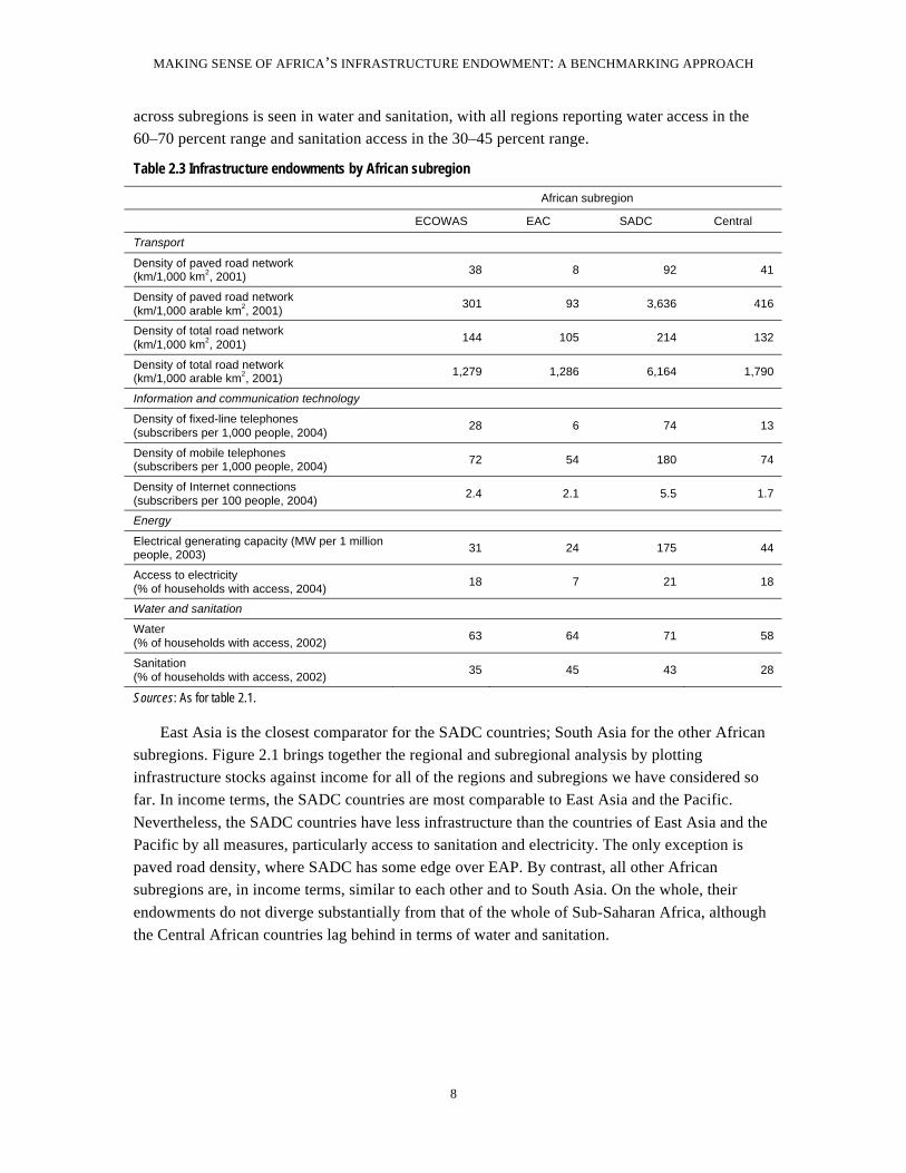
Nevertheless, the African average masks significant variations within the region (table 2.3).
To compare subregional endowments, we used four country groupings. They are SADC (all the
SADC countries except Tanzania); the East African Community (EAC) of Kenya, Tanzania, and
Uganda; the Economic Community of West African States (all the ECOWAS countries); and
Central Africa, a default category comprised of Burundi, Cameroon, the Central African
Republic, Chad, Comoros, Congo, Rep., Equatorial Guinea, Eritrea, Ethiopia, Gabon,
Madagascar, Mauritania, Mozambique, Rwanda, Sao Tome and Principe, Somalia and Sudan.
Comparing infrastructure endowments across these subregions reveals that the SADC
countries have a substantial advantage over the others. That advantage is most pronounced in the
case of paved roads, ICT, and power, where SADC is ahead of the other regions by several
multiples. Generating capacity (per capita) in SADC, for example, is more than five times that
reported in other parts of Africa, although, strikingly, household access to electricity is relatively
similar. At the other end of the spectrum, EAC has the lowest infrastructure endowment on most
measures. Western and central Africa are similar in their results. The least divergence in stocks
MAKING SENSE OF AFRICA’S INFRASTRUCTURE ENDOWMENT: A BENCHMARKING APPROACH
8
across subregions is seen in water and sanitation, with all regions reporting water access in the
60–70 percent range and sanitation access in the 30–45 percent range.
Table 2.3 Infrastructure endowments by African subregion
African subregion
ECOWAS EAC SADC Central
Transport
Density of paved road network (km/1,000 km
2, 2001)
38 8 92 41
Density of paved road network (km/1,000 arable km
2, 2001)
301 93 3,636 416
Density of total road network (km/1,000 km
2, 2001)
144 105 214 132
Density of total road network (km/1,000 arable km
2, 2001)
1,279 1,286 6,164 1,790
Information and communication technology
Density of fixed-line telephones (subscribers per 1,000 people, 2004)
28 6 74 13
Density of mobile telephones (subscribers per 1,000 people, 2004)
72 54 180 74
Density of Internet connections (subscribers per 100 people, 2004)
2.4 2.1 5.5 1.7
Energy
Electrical generating capacity (MW per 1 million people, 2003)
31 24 175 44
Access to electricity (% of households with access, 2004)
18 7 21 18
Water and sanitation
Water (% of households with access, 2002)
63 64 71 58
Sanitation (% of households with access, 2002)
35 45 43 28
Sources: As for table 2.1.
East Asia is the closest comparator for the SADC countries; South Asia for the other African
subregions. Figure 2.1 brings together the regional and subregional analysis by plotting
infrastructure stocks against income for all of the regions and subregions we have considered so
far. In income terms, the SADC countries are most comparable to East Asia and the Pacific.
Nevertheless, the SADC countries have less infrastructure than the countries of East Asia and the
Pacific by all measures, particularly access to sanitation and electricity. The only exception is
paved road density, where SADC has some edge over EAP. By contrast, all other African
subregions are, in income terms, similar to each other and to South Asia. On the whole, their
endowments do not diverge substantially from that of the whole of Sub-Saharan Africa, although
the Central African countries lag behind in terms of water and sanitation.

MAKING SENSE OF AFRICA’S INFRASTRUCTURE ENDOWMENT: A BENCHMARKING APPROACH
9
Figure 2.1 Infrastructure endowments plotted against national income, by world region
a. Percentage of households with improved water b. Percentage of households with improved sanitation
CENTRAL
EACECOWAS
SADC
EAP
ECA
LCR
MNA
SAS
SSA
60
70
80
90
0 1000 2000 3000 4000
Income Per-Capita
CENTRAL
EAC
ECOWAS
SADC
EAP
ECALCR MNA
SAS
SSA
30
40
50
60
70
80
0 1000 2000 3000 4000
Income Per-Capita
c. Percentage of households with electricity d. MW installed generating capacity per 1 million people
CENTRAL
EAC
ECOWASSADC
EAP
LCR
MNA
SAS
SSA
020
40
60
80
0 1000 2000 3000 4000
Income Per-Capita
CENTRALEACECOWAS
SADCEAP
ECA
LCRMNA
SAS
SSA0200
400
600
800
10
0 1000 2000 3000 4000
Income Per-Capita
e. Total roads (km/km2) f. Paved roads (km/km2)
CENTRALEAC
ECOWAS
SADCEAP
ECA
LCR
MNA
SAS
SSA
0200
400
600
80
0 1000 2000 3000 4000
Income Per-Capita
CENTRALEAC
ECOWAS
SADCEAP
ECA
LCR
MNA
SAS
SSA
0100
200
300
400
50
0 1000 2000 3000 4000
Income Per-Capita

MAKING SENSE OF AFRICA’S INFRASTRUCTURE ENDOWMENT: A BENCHMARKING APPROACH
10
Figure 2.1 Infrastructure endowments plotted against national income, by world region, continued
g. Mobile telephone subscribers per 1,000 inhabitants h. Landline telephone subscribers per 1,000 inhabitants
CENTRALEAC
ECOWAS
SADCEAP
ECA
LCR
MNA
SASSSA
0100
200
300
400
50
0 1000 2000 3000 4000
Income Per-Capita
CENTRALEAC
ECOWAS
SADCEAP
ECA
LCR
MNA
SASSSA
050
100
150
200
250
0 1000 2000 3000 4000
Income Per-Capita
Source: As for table 2.1.
Variations across types of countries
Relative to other developing regions, Sub-Saharan Africa faces a difficult environment for the
development of infrastructure, and the region’s infrastructure shortfall may be traceable to those
environmental disadvantages (table 2.4). Building infrastructure tends to be more difficult in
countries characterized by low population density and low levels of urbanization, weak
governance, high incidence of conflict, and geographical isolation—all of which distinguish
Africa from other developing regions. Africa has the lowest population density, the lowest
governance index, and the second-lowest urbanization rate of all developing regions. The
incidence of conflict in Africa is similar to that in other regions in percentage terms, but the
absolute number of countries in conflict is higher in Africa than in any other region.
Table 2.4 Difficulty of infrastructure environment across regions
Regional characteristic Su
b-S
ah
ara
n
Afr
ica
So
uth
Asia
Ea
st
Asia
an
d
Pa
cific
Eu
rop
e a
nd
C
en
tra
l A
sia
La
tin
Am
eri
ca
a
nd
Ca
rib
be
an
Mid
dle
Ea
st
an
d N
ort
h
Afr
ica
Population density (pop./km2) 67 436 121 71 133 150
Urbanization rate (%) 37 23 42 57 63 69
Governance index (0=most corrupt; 10=least corrupt) 3.7 4.3 4.2 3.9 3.8 4.5
Landlocked countries (%) 30 38 9 29 6 0
Countries in conflict (%) 23 25 14 25 12 25
Income per capita (US$) 999 842 1,801 3,628 3,649 4,193
Sources: As for table 2.1.
To explore the potential impact of environmental variables, we compare the infrastructure
endowment of countries within the region according to the difficulty of their environment. As

MAKING SENSE OF AFRICA’S INFRASTRUCTURE ENDOWMENT: A BENCHMARKING APPROACH
11
expected, countries facing a more challenging environment perform systematically worse on
infrastructure (table 2.5). The differences in endowment are largest for landlocked countries,
countries in conflict, and countries with low population density. Countries with low urbanization
perform worse on service coverage, but better on road density. Countries with poor governance
also perform worse than their comparators, but the differences are less pronounced. Overall,
paved road density is the infrastructure variable that shows the largest variation across types of
countries, while water and sanitation show the least variation.
Striking differences also emerge when countries are grouped according to their oil-exporting
status and language (table 2.6). Oil-exporting countries score systematically and substantially
worse than oil-importing countries, suggesting that oil revenues are not being channeled into
infrastructure investments. With respect to language groupings, francophone countries have the
lowest infrastructure stocks overall. Once again, the largest differences are to be found in the area
of paved road density, and the smallest in water and sanitation.

MAKING SENSE OF AFRICA’S INFRASTRUCTURE ENDOWMENT: A BENCHMARKING APPROACH
12
Table 2.5 Infrastructure endowments by demographic, political, and geographic variables
Population
density Urbanization Governance
Conflict status
Coastline
Sector and measure Low High Low High Poor Good Yes No No Yes
Transport
Density of paved road network (km/1,000 km
2, 2001)
11 131 51 21 45 54 12 62 16 65
Density of paved road network (km/1,000 arable km
2, 2001)
273 2,829 1,144 308 354 1,819 212 1,378 218 1,492
Density of total road network (km/1,000 km
2, 2001)
79 315 155 112 178 126 135 158 148 154
Density of total road network (km/1,000 arable km
2, 2001)
1,878 4,065 2,585 2,178 1,532 3,631 1,927 2,762 1,174 3,183
Information and communication technology
Density of fixed-line telephones (subscribers per 1,000 people, 2004)
21 56 33 28 10 51 15 36 14 50
Density of mobile telephones (subscribers per 1,000 people, 2004)
92 133 82 321 68 128 44 115 49 131
Density of Internet connections (subscribers per 100 people, 2004)
2.2 4.1 2.7 3.8 2.6 3.0 1.0 3.3 1.3 3.5
Energy
Electrical generating capacity (MW per 1 million people, 2003)
79 49 46 410 47 92 39 79 40 83
Access to electricity (% of households with access, 2004) 18 17 16 49 15 21 10 21 9 22
Water and sanitation
Water (% of households with access, 2002)
59 72 62 77 63 64 52 67 61 64
Sanitation (% of households with access, 2002)
34 39 34 48 35 35 27 38 32 36
Sources: As for table 2.1.
While the preceding analysis is suggestive, it does not take into account the high correlations
that exist among these different variables, and with income. Indeed, correlation coefficients
between these different indicators of “difficulty” range in absolute value between 0.3 and 0.6. In
order to isolate the effect of individual factors we must perform a multivariate regression analysis
that looks at all of the effects simultaneously.
As described in equation (1) above, we perform simple OLS cross-sectional analysis for each
category of infrastructure. Many control variables are considered—among them income per
capita; demographic measures (population density, urbanization, urban growth rates, and ethnic
fractionalization); measures of the quantity and quality of public spending on infrastructure
(proxied by governance and infrastructure aid per capita); measures capturing the geographical
and cultural heritage of the country (including language group, location, and natural resources);
and indicators of the structure of the economy (such as the share of exports, agriculture, and
manufacturing in GDP). In addition, an Africa dummy is used to see if any specific disadvantages
are associated with the continent as a whole.

MAKING SENSE OF AFRICA’S INFRASTRUCTURE ENDOWMENT: A BENCHMARKING APPROACH
13
Table 2.6 Infrastructure endowments by historical variables
Oil-exporter
Not oil exporter
Lusophone Anglophone Francophone
Transport
Density of paved road network (km/1,000 km
2, 2001)
14 57 95 84 31
Density of paved road network (km/1,000 arable km
2, 2001)
246 1,273 1,315 2,705 188
Density of total road network (km/1,000 km
2, 2001)
70 173 152 240 136
Density of total road network (km/1,000 arable km
2, 2001)
1,909 2,720 2,295 4,861 1,425
Information and communication technology
Density of fixed-line telephones (subscribers per 1,000 people, 2004)
16 38 148 48 4
Density of mobile telephones (subscribers per 1,000 people, 2004)
118 97 86 139 46
Density of Internet connections (subscribers per 100 people, 2004)
1.7 3.1 3.7 4.8 1.5
Energy
Electrical generating capacity (MW per 1 million people, 2003)
66 71 49 145 22
Access to electricity (% of households with access, 2004)
26 16 15 23 15
Water and sanitation
Water (% of households with access, 2002)
59 64 59 72 60
Sanitation (% of households with access, 2002)
34 35 35 46 29
Sources: As for table 2.1.
The OLS regression analysis reveals that levels of infrastructure stocks are primarily related
to per capita income and demographic variables, and less so to other variables (table 2.7). Income
is statistically significant in almost all cases, except for household access to water and electricity.
Demographic variables also seem to be important. Higher levels of urbanization are associated
with significantly higher rates of household access to water, sanitation, electricity. By contrast,
higher rates of urban growth significantly hold back rates of access to services, suggesting
difficulties in keeping up with the rate of urban expansion. Moreover, countries with higher
population density seem to have significantly less road area, although this difference disappears
when arable land is used to measure road density.
None of the other geographical, cultural, or structural variables prove to be statistically
significant in explaining infrastructure stocks. This suggests that in the earlier analysis, the
seeming effect of geographical and cultural variables was likely being confounded with the effect
of income and demographic variables with which they are associated. Finally, it is noteworthy
that the coefficients for infrastructure aid per capita and governance are rarely significant and do
not always have the expected signs.
An alternative log-log specification of the model, designed to test the sensitivity of the
estimates, yields similar results, while revealing relatively low income elasticities and somewhat

MAKING SENSE OF AFRICA’S INFRASTRUCTURE ENDOWMENT: A BENCHMARKING APPROACH
14
higher urbanization elasticities (table 2.8). The main differences from the first OLS model are
these: In the log-log model, income is no longer significant for road density, and some of the
structural variables (exports, agriculture, manufacturing) become more significant. Overall, the fit
of the model is also somewhat improved. The log-log specification also allows the coefficients on
continuous variables to be interpreted as elasticities. The results suggest that the income elasticity
of infrastructure stocks is generally well below unity, with the highest values (around 0.5 to 0.7)
found for ICT and generating capacity and the lowest (around 0.1 to 0.2) for access to water,
sanitation, and electricity, and for roads. The elasticity of urbanization is somewhat higher,
particularly for access to electricity and ICT services.
In summary, Africa presents a major infrastructure deficit relative to other developing regions
that appears to reflect low urbanization as much as low income. The region lags behind all others
in the developing world in almost all areas of infrastructure. The strongest endowments are found
in the ICT sector, where Africa is somewhat ahead of South Asia. By far the lowest endowment is
in the power sector. Rates of access to electricity in the middle-income countries of Africa, for
example, are a fraction of those found in middle-income countries in other regions.
The regional average masks significant geographic variations in infrastructure endowments
from country to country. The SADC countries are substantially ahead of the others, while the
EAC countries are significantly behind.
Africa’s deficit remains even when countries are compared with others in the same income
bracket. The reason appears to be that—compared with other regions of the world—Africa is a
difficult environment in which to develop infrastructure. The proof is that infrastructure is
weakest in those countries that face the most challenging environment. However, some
environmental factors are more important than others. When all environmental variables are
considered simultaneously, demographic variables (notably urbanization) appear to have the most
substantial effect on infrastructure endowments.

MAKING SENSE OF AFRICA’S INFRASTRUCTURE ENDOWMENT: A BENCHMARKING APPROACH
15
Table 2.7 Effect of country variables on infrastructure endowments, part 1
Cross-sectional OLS analysis, data in levels
Variable De
nsity o
f ro
ad
s
De
nsity o
f ro
ad
s
(ara
ble
)
De
nsity o
f p
ave
d r
oa
ds
De
nsity o
f p
ave
d r
oa
ds
(ara
ble
)
Acce
ss t
o
wa
ter
Acce
ss t
o
sa
nita
tio
n
Acce
ss t
o
ele
ctr
icity
Ge
ne
ratin
g
ca
pa
city
Inte
rne
t co
nn
ectio
ns
Mo
bile
te
lep
ho
ne
s
Fix
ed
-lin
e
tele
ph
on
es
0.0001 0.002 0.0001 0.001 0.001 0.003 0.001 0.0001 0.003 0.056 0.021 Income per capita (5.73)** (3.07)** (4.20)** (3.15)** –0.66 (2.76)** –0.84 (4.87)** (5.25)** (5.75)** (5.37)**
–0.515 –8.845 –0.288 –2.697 26.93 40.957 63.355 0.345 3.878 105.594 97.429 Urbanization
–1.66 –1.16 –1.06 –0.85 (2.66)** (3.31)** (4.81)** –1.55 –0.59 –0.82 –1.89
0.001 –0.007 0.002 0.003 0.031 0.007 0.019 –0.0001 0.01 –0.004 0.074 Population density (4.29)** –0.87 (5.53)** –0.84 (3.04)** –0.55 –1.4 –0.56 –1.49 –0.03 –1.36
–0.052 0.451 –0.061 –0.052 –2.081 –4.273 –3.097 –0.095 –0.485 –16.292 –15.805 Urban growth
–1.92 –0.67 (2.55)* –0.19 (2.23)* (3.66)** (2.11)* (4.62)** –0.82 –1.43 (3.34)**
0.036 –1.447 –0.048 –2.14 0.567 4.632 14.682 0.297 –0.583 71.167 –9.624 Fractionali-zation –0.23 –0.38 –0.36 –1.37 –0.11 –0.72 (2.23)* (2.56)* –0.18 –1.08 –0.36
0.003 –0.197 0.005 0.198 0.507 –0.4 –0.717 –0.011 0.283 –6.042 0.024 Governance
–0.15 –0.39 –0.29 –0.96 –0.74 –0.46 –0.73 –0.74 –0.66 –0.74 –0.01
0.002 0.003 –0.002 –0.032 0.035 0.263 0.231 0.0004 –0.059 0.635 0.55 Infrastructure aid (per capita) –0.89 –0.07 –1.34 –1.81 –0.62 (3.76)** (2.15)* –0.33 –1.38 –0.72 –1.69
–0.119 –1.954 0.034 1.226 –7.198 –19.246 –35.293 –0.198 –2.237 –73.992 –29.09 Africa
–1.03 –0.69 –0.34 –1.05 –1.95 (4.27)** (7.13)** (2.37)* –0.89 –1.39 –1.42
0.141 3.394 –0.001 1.001 –3.101 7.351 –5.68 –0.103 0.088 8.696 –1.339 Anglophone
–1.1 –1.08 –0.01 –0.78 –0.73 –1.41 –1.04 –1.08 –0.03 –0.15 –0.06
0.043 –0.113 0.061 0.01 –6.511 –0.918 1.79 –0.034 1.266 28.44 –2.927 Francophone
–0.36 –0.04 –0.59 –0.01 –1.68 –0.2 –0.39 –0.39 –0.5 –0.55 –0.14
0.012 –0.864 0.041 –0.397 –1.434 –2.953 –4.667 0.075 –0.131 20.189 –0.019 Landlocked
–0.12 –0.36 –0.49 –0.4 –0.44 –0.75 –1 –1.06 –0.06 –0.47 0
–0.109 0.698 0.037 0.213 –3.356 –6.323 5.269 0.001 –3.03 –53.872 –15.892 Oil-exporting
–1.25 –0.33 –0.48 –0.24 –1.15 –1.79 –1.35 –0.01 –1.65 –1.48 –1.08
0.09 0.104 0.003 –0.173 –6.223 5.548 –2.748 –
0.0001 –2.37 4.995 –2.097
Conflict
–0.85 –0.04 –0.03 –0.16 –1.84 –1.36 –0.58 0.0766 –1.08 –0.11 –0.12
–0.0003 0.07 0.0004 0.038 –0.099 –0.068 –0.131 0.001 0.114 1.497 –0.029 Exports (% GDP) –0.15 –1.29 –0.2 –1.75 –1.38 –0.71 –1.44 –0.63 (2.45)* –1.62 –0.08
0.002 –0.056 0.003 –0.004 –0.164 0.192 –0.196 0.006 0.052 –1.379 0.578 Agriculture (% GDP) –0.52 –0.49 –0.71 –0.09 –1.05 –1.02 –1 –1.63 –0.52 –0.64 –0.73
–0.008 –0.275 –0.006 –0.062 –0.294 0.113 0.572 0.002 0.138 2.601 0.304 Manufacturing (% GDP) –1.21 –1.79 –1.04 –0.96 –1.47 –0.46 –1.98 –0.56 –1.05 –0.97 –0.29
0.343 7.331 0.126 0.385 81.37 45.274 38.376 0.092 –4.259 44.459 41.711 Constant
–1.13 –0.99 –0.48 –0.13 (8.18)** (3.51)** (2.93)** –0.42 –0.66 –0.35 –0.84
Observations 105 104 104 103 101 99 82 110 108 93 107
R–squared 0.62 0.28 0.55 0.35 0.61 0.74 0.87 0.69 0.63 0.74 0.74
Note: * = significant at 5%; ** = significant at 10%. T-statistics are reported below coefficients. Parentheses denote that T-statistics
have been reported in absolute value.

MAKING SENSE OF AFRICA’S INFRASTRUCTURE ENDOWMENT: A BENCHMARKING APPROACH
16
Table 2.8 Effect of country variables on infrastructure endowments, part 2
Cross-sectional OLS analysis, data in logs (except dummy variables, which are in levels)
Variable De
nsity o
f ro
ad
s
De
nsity o
f ro
ad
s
(ara
ble
)
De
nsity o
f p
ave
d r
oa
ds
De
nsity o
f p
ave
d r
oa
ds
(ara
ble
)
Acce
ss t
o
wa
ter
Acce
ss t
o
sa
nita
tio
n
Acce
ss t
o
ele
ctr
icity
Ge
ne
ratin
g
ca
pa
city
Inte
rne
t co
nn
ectio
ns
Mo
bile
te
lep
ho
ne
s
Fix
ed
-lin
e
tele
ph
on
es
0.112 0.262 0.082 0.222 0.135 0.041 –0.061 0.451 0.693 0.492 0.748 Income per capita (2.87)** (2.93)** –0.57 –1.65 –0.75 –0.2 –0.27 (2.30)* (5.19)** (3.05)** (5.13)**
0.188 0.461 0.991 0.341 0.426 –0.126 –0.023 0.942 0.885 0.859 0.54 Urbanization
(3.19)** (3.40)** (4.93)** –1.62 –1.5 –0.38 –0.06 (3.05)** (4.07)** (3.53)** (2.29)*
0.071 0.081 0.09 0.729 1.111 –0.036 0.341 0.193 0.062 –0.048 0.121 Population density (4.80)** (2.38)* –1.72 (14.12)** (16.12)** –0.44 (3.95)** (2.57)* –1.18 –0.75 (2.11)*
–0.07 –0.149 –0.181 –0.208 –0.598 0.201 –0.205 –0.243 –0.138 –0.488 –0.346 Urban growth
(2.26)* (2.04)* –1.46 (2.23)* (4.76)** –1.39 –1.31 –1.72 –1.53 (4.42)** (3.28)**
–0.011 –0.018 0.047 –0.088 –0.013 –0.146 –0.073 –0.019 –0.022 0.08 –0.08 Fractionali- zation –0.69 –0.51 –0.88 –1.61 –0.18 –1.72 –0.81 –0.24 –0.4 –1.28 –1.37
0.035 0.034 0.086 –0.308 –0.122 –0.259 –0.05 –0.191 –0.339 0.016 0.035 Governance
–0.81 –0.33 –0.55 (2.09)* –0.62 –1.13 –0.2 –0.88 (2.43)* –0.09 –0.22
–0.006 0.023 0.033 0.008 –0.006 0.025 0.009 0.002 0.067 –0.016 0.019 Infrastructure aid (per capita) –0.67 –1.05 –0.99 –0.27 –0.14 –0.54 –0.17 –0.04 (2.24)* –0.45 –0.57
–0.05 –0.251 –0.871 –0.097 –0.029 –0.249 –0.169 –0.042 –0.003 –0.998 –0.451 Africa
–1.01 (2.19)* (5.14)** –0.55 –0.12 –0.9 –0.57 –0.16 –0.02 (4.93)** (2.26)*
–0.024 0.265 –0.135 0.526 –0.214 0.565 –0.144 0.039 0.269 0.246 –0.364 Anglophone
–0.44 (2.13)* –0.73 (2.81)** –0.85 –1.94 –0.46 –0.14 –1.4 –1.08 –1.67
–0.153 –0.23 –0.075 –0.11 –0.322 –0.347 –0.53 –0.331 –0.057 –0.621 –0.825 Francophone
(3.01)** –1.96 –0.45 –0.61 –1.33 –1.24 –1.76 –1.26 –0.31 (2.95)** (4.19)**
0.018 0.059 –0.221 0.314 –0.107 0.016 –0.474 –0.04 0.142 0.107 –0.076 Landlocked
–0.36 –0.52 –1.18 –1.92 –0.48 –0.06 –1.67 –0.16 –0.89 –0.54 –0.42
–0.017 –0.033 0.195 –0.453 –0.001 –0.305 0.156 –0.294 –0.014 0.005 0.002 Oil exporting
–0.41 –0.34 –1.34 (3.06)** 0 –1.32 –0.63 –1.37 –0.1 –0.03 –0.01
–0.091 0.011 –0.109 0.088 –0.347 0.002 –0.425 –0.272 0.171 –0.169 –0.286 Conflict
–1.98 –0.11 –0.66 –0.54 –1.58 –0.01 –1.55 –1.15 –1.08 –0.89 –1.62
–0.078 0.079 –0.015 0.365 0.479 0.585 0.666 0.444 0.474 0.285 0.034 Exports (% GDP) (2.18)* –0.92 –0.12 (2.86)** (2.82)** (2.92)** (3.12)** (2.42)* (3.88)** –1.93 –0.24
0.081 0.296 0.07 –0.031 –0.124 –0.759 –0.864 0.114 0.231 0.265 0.344 Agriculture (% GDP) –1.88 (2.97)** –0.47 –0.21 –0.63 (3.33)** (3.52)** –0.53 –1.57 –1.45 (2.13)*
–0.064 0.04 0.142 –0.148 –0.193 –0.367 –0.428 0.014 0.089 0.035 –0.033 Manufacturing (% GDP) –1.79 –0.47 –1.12 –1.17 –1.13 –1.86 (2.01)* –0.07 –0.67 –0.24 –0.23
3.706 1.111 3.526 –6.44 –8.298 1.309 –0.262 –3.128 –1.791 –5.408 –2.015 Constant
(9.19)** –1.16 (2.41)* (4.59)** (4.39)** –0.6 –0.11 –1.56 –1.35 (3.19)** –1.34
Observations 94 92 82 95 95 94 94 98 84 98 97
R–squared 0.71 0.69 0.81 0.85 0.87 0.55 0.69 0.7 0.87 0.86 0.87
Note: * = significant at 5%; ** = significant at 10%. T-statistics are reported below coefficients. Parentheses denote that T-statistics
have been reported in absolute value.
MAKING SENSE OF AFRICA’S INFRASTRUCTURE ENDOWMENT: A BENCHMARKING APPROACH
17
3 The impact of historical trends on
infrastructure endowments
Variations over time
Africa’s present-day infrastructure is strongly influenced by the endowment that the countries
inherited at independence. Because infrastructure is costly to build, stocks usually change slowly
over time. Hence, differences across developing regions will reflect differences in their history.
The current dataset contains time series data going back as far as 1960 for roads, 1970 for fixed
telephone lines, 1980 for generating capacity, and 1990 for water and sanitation. No consistent
time series data are available for access to electricity. The data points from the 1960s and 1970s
are of particular interest for Africa, since they describe the situation at around the time of
independence.
Overall, the data show some evidence of worldwide convergence in infrastructure levels
(table 3.1). They also reveal the divergent starting points and differing rates of infrastructure
growth in world regions. Convergence requires, of course, that regions with a low starting point
grow faster than regions with a high starting point. We computed correlation coefficients between
starting levels and growth rates. These coefficients are uniformly negative and always smaller
than –0.28, suggesting that convergence is underway. The strongest evidence of convergence is
found for water and sanitation (with correlation coefficients between –0.6 and –0.7) and roads
(with correlation coefficients between –0.45 and –0.55). The lowest is for generating capacity
(with a correlation coefficient of –0.28).
Bucking the trend toward worldwide convergence, the infrastructure gap between Africa and
other developing regions is larger today than it was some decades ago. Slow convergence has
occurred for some forms of infrastructure. At the beginning of the data series for paved roads and
access to water and sanitation, Africa had the lowest endowment of any developing region. The
region managed to achieve relatively high growth rates in each category, but they were not great
enough to compensate for the region’s starting position. On the other hand, at the outset of the
data series, Africa was doing significantly better than other developing regions with regard to
overall road density, generation capacity, and fixed-line telephones. But growth rates in these
categories have been slower than in other regions, so that by 2000 Africa had lost substantial
ground relative to the other regions.
Africa’s failure to converge with the rest of the developing world is most clearly illustrated
by the comparison between Africa and South Asia. At the outset of the period under study, South
Asia was ahead of Africa in all forms of infrastructure except for fixed-line telephones and
electrical generating capacity (figure 3.1). Their positions have since been reversed. The record
on generating capacity is particularly stark. In 1980, Africa had almost three times as much
generating capacity (per million people) as South Asia. Since then, capacity in South Asia has
expanded at an average annual rate of 9 percent, while in Africa it has stagnated. Consequently,

MAKING SENSE OF AFRICA’S INFRASTRUCTURE ENDOWMENT: A BENCHMARKING APPROACH
18
by 1990 South Asia had overtaken Africa; by 2000 it had almost twice the generating capacity
(per million people) of Africa. Indeed, Africa had the slowest rate of growth in generating
capacity of any region in the developing world. The story for telephone lines is similar, if less
dramatic. In 1970, Africa had twice the teledensity of South Asia. However, with faster average
annual growth rates in South Asia (9 percent against 6 percent in Africa), the two regions had
converged by 2000. Africa has now fallen behind South Asia with respect to fixed-line
telephones, but in mobile telephony and Internet connections Africa has been growing more
rapidly than South Asia and currently maintains a lead.
Indexing infrastructure stocks in each region and plotting the evolution of the indexes over
time sheds light on the sequencing and relative growth path of different aspects of infrastructure.
In all regions, fixed-line telephones have been by far the fastest-growing component of
infrastructure since the 1980s (albeit from low starting points), but the growth varies substantially
across regions from around tenfold in Africa, Latin America, and the Middle East, to more than
forty-fold in East Asia (figure 3.2). After telephone lines, paved roads generally have expanded
most quickly, particularly in East Asia and Eastern Europe. Generating capacity (per million
people) has grown only very slowly across all regions, except in South Asia in the late 1980s,
when a significant expansion took place.
Within Africa, the SADC countries started with a larger infrastructure endowment than the
other subregions and extended it more rapidly (table 3.2). At independence there already were
substantial variations in infrastructure endowment across the continent—particularly with respect
to paved roads, generating capacity, and telephone lines. By 1980, the SADC countries had more
than three times the generating capacity of other subregions. By 1970, they had five times the
teledensity. In the case of roads, ECOWAS was in a much stronger position than the other
subregions in the 1960s, but was overtaken by SADC after 1980. In water and sanitation, the
differences between subregions have been relatively small.

MAKING SENSE OF AFRICA’S INFRASTRUCTURE ENDOWMENT: A BENCHMARKING APPROACH
19
Table 3.1 Trends in infrastructure endowments, by world region, 1960–2000
Region 1960 1970 1980 1990 2000 a
Average annual growth
b
(percent)
SSA 6 8 21 26 39 5.0
SAS 60 76 115 113 146 2.3
EAP 12 21 37 39 54 4.0
ECA 54 239 312 362 351 4.9
LAC 132 185 59 274 361 2.6
Density of paved road network (km/1,000 km
2)
MNA 14 19 26 39 45 3.1
SSA 71 120 544 652 1,037 7.1
SAS 477 434 585 711 670 0.9
EAP 239 392 563 453 556 2.2
ECA 110 498 687 800 1,197 6.3
LAC 472 808 527 1,973 3,958 5.6
Density of paved road network (km/1,000 arable km
2)
MNA 196 320 3,283 4,594 5,729 9.0
SSA 73 80 106 119 143 1.7
SAS 104 145 204 204 303 2.8
EAP 55 75 144 157 175 3.0
ECA 298 576 567 630 620 1.9
LAC 267 198 241 516 583 2.0
Density of total road network (km/1,000 km
2)
MNA 45 50 77 92 104 2.2
SSA 1,525 1,577 2,106 2,343 2,556 1.3
SAS 757 699 888 1,084 1,408 1.6
EAP 3,064 2,671 3,244 3,063 3,252 0.2
ECA 651 1,188 1,261 1,543 2,045 3.0
LAC 1,962 2,138 2,743 4,929 7,021 3.3
Density of total road network (km/1,000 arable km
2)
MNA 558 760 33,263 28,850 30,704 10.8
SSA — 4 7 11 22 5.6
SAS — 2 2 5 21 8.9
EAP — 5 10 21 58 8.9
ECA — 32 76 134 229 6.8
LAC — 24 44 75 155 6.4
Density of fixed-line telephones (subscribers per 1,000 people)
MNA — 9 18 41 84 7.7
SSA — — 71 82 73 0.1
SAS — — 26 127 137 8.6
EAP — — 123 178 229 3.2
ECA — — 587 786 1,022 2.8
LAC — — 309 409 495 2.4
Electrical generating capacity (MW per 1 million people)
MNA — — 207 421 413 3.5
SSA — — — 51 63 1.0
SAS — — — 72 70 –0.2
EAP — — — 73 73 –0.03
ECA — — — 93 89 –0.4
LAC — — — 81 89 0.7
Water (% of households with access)
MNA — — — 83 83 –0.02

MAKING SENSE OF AFRICA’S INFRASTRUCTURE ENDOWMENT: A BENCHMARKING APPROACH
20
SSA — — — 30 35 0.4
SAS — — — 31 47 1.3
EAP — — — 57 53 –0.4
ECA — — — 86 80 –0.5
LAC — — — 64 76 1.0
Sanitation (% of households with access)
MNA — — — 69 75 0.5
Sources: As for table 2.1.
Note: SSA = Sub-Saharan Africa, SAS = South Asia, EAP = East Asia and Pacific, ECA = Europe and Central Asia, LAC = Latin America and Caribbean, MNA = Middle East and North Africa.
a. Water and sanitation data are from 2002.
b. Calculated over entire period available for each sector.
— = data not available.

MAKING SENSE OF AFRICA’S INFRASTRUCTURE ENDOWMENT: A BENCHMARKING APPROACH
21
Table 3.2 Trends in infrastructure endowments by African subregion, 1960–2000
1960 1970 1980 1990 2000 a
Average annual growth
b
(percent)
Central Africa 1 2 5 8 9 6
EAC 3 6 12 13 8 3
ECOWAS 11 14 21 24 38 3
Density of paved road network (km/1,000 km
2)
SADC 4 9 46 53 92 8
Central Africa 19 75 156 161 159 6
EAC 46 106 135 148 95 2
ECOWAS 122 161 213 237 305 2
Density of paved road network (km/1,000 arable km
2)
SADC 64 123 1,715 2,015 3,649 11
Central Africa 57 60 82 94 101 1
EAC 56 77 82 94 105 2
ECOWAS 84 93 109 121 144 1
Density of total road network (km/1,000 km
2)
SADC 81 90 140 154 211 2
Central Africa 2,101 1,720 1,776 1,677 1,587 –1
EAC 1,053 1,201 1,073 1,124 1,297 1
ECOWAS 1,137 1,259 1,391 1,319 1,300 0.3
Density of total road network (km/1,000 arable km
2)
SADC 1,588 2,058 4,002 5,045 6,174 4
Central Africa — 1 2 4 7 5
EAC — 2 3 4 6 4
ECOWAS — 2 3 5 17 8
Density of fixed-line telephones (subscribers per 1,000 people)
SADC — 10 18 32 56 6
Central Africa — — 49 57 48 –0.1
EAC — — 21 20 23 0.4
ECOWAS — — 38 34 31 –1
Electrical generating capacity (MW per 1 million people)
SADC — — 177 204 185 0.2
Central Africa — — — 46 56 1
EAC — — — 42 64 2
ECOWAS — — — 51 63 1
Water (% of households with access)
SADC — — — 60 73 1
Central Africa — — — 22 27 0.5
EAC — — — 44 45 0.1
ECOWAS — — — 28 35 1
Sanitation (% of households with access)
SADC — — — 37 42 0.4
Sources: As for table 2.1.
a. Water and sanitation data are from 2002.
b. Calculated over entire period available for each sector.
— = data not available.

MAKING SENSE OF AFRICA’S INFRASTRUCTURE ENDOWMENT: A BENCHMARKING APPROACH
22
Figure 3.1 Index of infrastructure growth by sector and by region
Tot. Rd. Density - Indexes Relative to SSA
0
200
400
600
800
1,000
1,200
1,400
1,600
1960 1965 1970 1975 1980 1985 1990 1995 2000
SSA
EAP
ECA
LCR
MNA
SAS
Paved Rd. Density - Indexes Relative to SSA
0
5,000
10,000
15,000
20,000
25,000
1960 1965 1970 1975 1980 1985 1990 1995 2000
SSA
EAP
ECA
LCR
MNA
SAS
Mainline Density - Indexes Relative to SSA
0
1,000
2,000
3,000
4,000
5,000
6,000
7,000
1975 1980 1985 1990 1995 2000
SSA
EAP
ECA
LCR
MNA
SAS
Mobile Density - Indexes Relative to SSA
0
50,000
100,000
150,000
200,000
250,000
300,000
350,000
1990
1992
1994
1996
1998
2000
2002
2004
SSA
EAP
ECA
LCR
MNA
SAS
Internet Density - Indexes Relative to SSA
0
2,000
4,000
6,000
8,000
10,000
12,000
14,000
16,000
1993
1994
1995
1996
1997
1998
1999
2000
2001
2002
2003
2004
SSA
EAP
ECA
LCR
MNA
SAS
Generation Capacity - Indexes Relative to SSA
0
200
400
600
800
1,000
1,200
1,400
1,600
1980 1985 1990 1995 2000
SSA
EAP
ECA
LCR
MNA
SAS
Water Access - Indexes Relative to SSA
0
20
40
60
80
100
120
140
160
180
200
SSA EAP ECA LCR MNA SAS
1990
2002
Sanitation Access - Indexes Relative to SSA
0
50
100
150
200
250
300
350
SSA EAP ECA LCR MNA SSA
1990
2002
Sources: As for table 2.1.

MAKING SENSE OF AFRICA’S INFRASTRUCTURE ENDOWMENT: A BENCHMARKING APPROACH
23
Figure 3.2 Indexes of infrastructure growth by region, 1960–2003
Index of Infrastructure Growth - SSA
0
200
400
600
800
1,000
1,200
1,400
1,600
1,800
2,000
1960 1965 1970 1975 1980 1985 1990 1995 2000
Paved Road
Tot. Road
Gen. Cap.
Mainline
Index of Infrastructure Growth - SAS
0
200
400
600
800
1,000
1,200
1,400
1,600
1,800
2,000
1960 1965 1970 1975 1980 1985 1990 1995 2000
Paved Road
Tot. Road
Gen. Cap.
Mainline
Index of Infrastructure Growth - EAP
0
200
400600
800
1,000
1,200
1,4001,600
1,800
2,000
1960 1965 1970 1975 1980 1985 1990 1995 2000
Paved Road
Tot. Road
Gen. Cap.
Mainline
Index of Infrastructure Growth - ECA
0
200
400
600
800
1,000
1,200
1,400
1,600
1,800
2,000
1960 1965 1970 1975 1980 1985 1990 1995 2000
Paved Road
Tot. Road
Gen. Cap.
Mainline
Index of Infrastructure Growth - LCR
0
200
400
600
800
1,000
1,200
1,400
1,600
1,800
2,000
1960 1965 1970 1975 1980 1985 1990 1995 2000
Paved Road
Tot. Road
Gen. Cap.
Mainline
Index of Infrastructure Growth - MNA
0
200
400
600
800
1,000
1,200
1,400
1,600
1,800
2,000
1960 1965 1970 1975 1980 1985 1990 1995 2000
Paved Road
Tot. Road
Gen. Cap.
Mainline
Sources: As for table 2.1.
Panel data models
The preceding exploratory data analysis illustrated the importance of historical perspective in
understanding countries’ present-day infrastructure position. We use panel data models to
integrate that perspective into our formal analysis. As described in the first section of this paper,
two different panel model specifications are estimated: an OLS fixed effects model and an
instrumental variables specification. Unfortunately, it is not possible to apply either of the panel
data models to access to electricity, for which only a single cross-section is available. (However,
we do apply a cross-sectional instrumental variables specification to the electricity access data so
as to compare them to the OLS estimates. That comparison is reported in table 3.4.)
The fixed effects model confirms the importance of income, demography, and economic
structure in driving stocks of household services and broader economic infrastructure (table 3.3).

MAKING SENSE OF AFRICA’S INFRASTRUCTURE ENDOWMENT: A BENCHMARKING APPROACH
24
The income and demographic variables that proved statistically significant in the cross-sectional
OLS results were also statistically significant in the fixed effects panel results. To a greater extent
than before, however, variables capturing the economic structure of the economy (export
orientation, and shares of agriculture and manufacturing compared with services) become
statistically significant in explaining infrastructure stocks, particularly in the case of roads and
ICT. It is important to remember, however, that these results do not yet account for dynamics in
infrastructure provision, nor have they been corrected for endogeneity.
Table 3.3 Results of OLS fixed effects panel data model
Data in logs
Variable De
nsity o
f ro
ad
s
De
nsity o
f ro
ad
s (
ara
ble
)
De
nsity o
f p
ave
d r
oa
ds
De
nsity o
f p
ave
d r
oa
ds
(ara
ble
)
Acce
ss t
o w
ate
r
Acce
ss t
o
sa
nita
tio
n
Acce
ss t
o
ele
ctr
icity
Ge
ne
ratin
g
ca
pa
city
Inte
rne
t co
nn
ectio
ns
Mo
bile
te
lep
ho
ne
s
Fix
ed
-lin
e
tele
ph
on
es
0.051 0.079 0.196 0.227 –0.022 0.126 0.371 0.247 1.768 2.059 0.633 Income
(3.25)** (4.49)** (10.60)** (11.15)** –0.47 –1.33 (2.52)* (11.87)** (7.73)** (11.77)** (27.68)**
0.244 0.131 0.477 0.365 0.664 0.141 1.096 0.504 2.316 3.158 0.986 Urbanization
(3.52)** –1.69 (5.90)** (4.10)** (3.30)** –0.36 (5.11)** (5.50)** (2.88)** (4.72)** (10.98)**
0.366 0.094 0.587 0.312 0.103 1.01 0.119 0.062 21.884 16.909 1.524 Population density (6.43)** –1.48 (8.76)** (4.24)** –0.64 (3.12)** (2.18)* –0.84 (26.44)** (25.86)** (20.14)**
–0.005 –0.011 –0.011 –0.017 –0.004 0.019 0.006 0.003 –0.019 0.08 –0.003 Infrastructure aid (per capita) –1.87 (3.90)** (3.76)** (5.08)** –0.54 –1.25 –0.17 –0.96 –0.8 (3.98)** –0.85
0.001 0 0.001 0.001 0.001 0 0.04 0.004 0.073 0.034 0.006 Exports (% GDP) –1.13 –0.35 (2.20)* –1.82 –0.35 –0.01 –0.29 (5.98)** (11.28)** (6.85)** (8.60)**
–0.004 –0.003 0.001 0.002 –0.001 0.009 0.188 –0.005 –0.112 –0.154 –0.01 Agriculture (% GDP) (3.40)** (2.58)** –0.95 –1.38 –0.49 –1.43 –1.17 (3.29)** (7.11)** (11.30)** (5.69)**
0.001 0.002 –0.001 0.001 –0.007 0.01 0.398 0.004 –0.151 –0.205 –0.002 Manufacturing (% GDP) –0.85 –1.43 –0.37 –0.27 –1.56 –1.13 (2.85)** (2.23)* (7.55)** (13.39)** –0.99
–3.401 –0.185 –6.602 –3.424 4.764 –1.021 –0.22 –10.59 –92.962 –70.033 –5.856 Constant
(11.67)** –0.57 (19.38)** (9.13)** (5.72)** –0.61 –0.15 (27.63)** (23.72)** (23.53)** (14.93)**
Observations 1919 1910 1875 1866 167 165 85 2223 1100 1230 2323
Plant fixed effects 0.21 0.07 0.39 0.24 0.67 0.52 0.68 0.22 0.68 0.76 0.73
Sources: As for table 2.1.
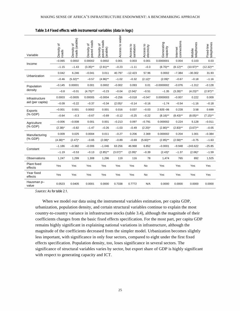
The results from the instrumental variables estimation indicate endogeneity bias in the OLS
specification. If—as suggested by Calderón and Servén (2004) and others that expansion of
infrastructure is associated with higher levels of income and growth, then we would expect the
OLS coefficient on per capita GDP to be upwardly biased. Indeed, the results of our instrumental
variables estimation show that the magnitude of the coefficient on per capita GDP decreased
substantially once we controlled for endogeneity using the standard regressors from the growth
literature, as discussed above. The traditional Hausman test of the exogeneity of our instruments
indicates that they are appropriate in most infrastructure sectors. The exception is in the estimates
for access to water and sanitation, where the limited number of observations (from just two years
of data) may have affected the results. But it is clear that addressing the endogeneity of per capita
GDP is critical to obtaining consistent coefficient estimates.
MAKING SENSE OF AFRICA’S INFRASTRUCTURE ENDOWMENT: A BENCHMARKING APPROACH
25
Table 3.4 Fixed effects with instrumental variables (data in logs)
Variable De
nsity o
f ro
ad
s
De
nsity o
f ro
ad
s (
ara
ble
)
De
nsity o
f p
ave
d r
oa
ds
De
nsity o
f p
ave
d r
oa
ds
(ara
ble
)
Acce
ss t
o w
ate
r
Acce
ss t
o
sa
nita
tio
n
Acce
ss t
o
ele
ctr
icity
Ge
ne
ratin
g
ca
pa
city
Inte
rne
t co
nn
ectio
ns
Mo
bile
te
lep
ho
ne
s
Fix
ed
-lin
e
tele
ph
on
es
–0.065 0.0002 0.00002 0.0002 0.001 0.003 0.001 0.0000001 0.004 0.103 0.03 Income
–1.15 –1.43 (3.35)** (2.91)** –0.23 –1.11 –0.3 (8.70)** (8.12)** (10.97)** (12.32)**
0.042 6.246 –0.041 3.011 40.797 –12.423 57.96 0.0002 –7.384 –30.302 31.93 Urbanization
–0.46 (5.32)** –0.57 (4.96)** –1.02 –0.32 (2.12)* (2.09)* –0.67 –0.18 –1.16
–0.145 0.00001 0.001 0.0002 –0.002 0.093 0.01 –0.0000002 –0.076 –1.312 –0.128 Population density –0.8 –0.01 (4.75)** –0.23 –0.04 (2.04)* –0.51 –1.35 (3.28)** (4.23)** (2.97)**
0.0003 –0.0005 0.00005 –0.0004 –0.256 –0.018 –0.047 0.0000003 –0.007 0.222 0.009 Infrastructure aid (per capita) –0.09 –0.22 –0.37 –0.34 (2.05)* –0.14 –0.16 –1.74 –0.54 –1.16 –0.18
–0.001 0.001 0.0002 0.001 0.016 0.037 –0.03 2.92E–06 0.228 3.58 0.699 Exports (% GDP) –0.64 –0.3 –0.67 –0.69 –0.12 –0.25 –0.22 (8.16)** (8.43)** (8.05)** (7.15)**
–0.006 –0.008 0.001 0.001 –0.213 0.097 –0.791 0.000002 0.224 5.128 –0.011 Agriculture (% GDP) (2.38)* –0.82 –1.47 –0.26 –1.03 –0.49 (2.20)* (2.80)** (2.83)** (3.67)** –0.05
0.009 0.025 0.0004 0.011 –0.27 0.206 2.369 0.000002 0.204 1.001 –0.384 Manufacturing (% GDP) (4.38)** (2.47)* –0.65 (2.08)* –0.89 –0.69 (5.60)** (2.85)** (2.58)** –0.75 –1.63
–1.186 –0.382 –0.006 –1.046 63.256 46.968 6.852 –0.0001 –9.948 –243.622 –25.85 Constant
–1.19 –0.53 –0.13 (2.85)** (3.07)** (2.09)* –0.39 (2.43)* –1.37 (2.06)* –1.59
Observations 1,247 1,299 1,308 1,296 119 116 78 1,474 765 892 1,525
Plant fixed effects
Yes Yes Yes Yes Yes Yes No Yes Yes Yes Yes
Year fixed effects
Yes Yes Yes Yes Yes Yes No Yes Yes Yes Yes
Hausman p–value
0.0523 0.0405 0.0001 0.0000 0.7338 0.7772 N/A 0.0000 0.0000 0.0000 0.0000
Sources: As for table 2.1.
When we model our data using the instrumental variables estimation, per capita GDP,
urbanization, population density, and certain structural variables continue to explain the most
country-to-country variance in infrastructure stocks (table 3.4), although the magnitude of their
coefficients changes from the basic fixed effects specification. For the most part, per capita GDP
remains highly significant in explaining national variations in infrastructure, although the
magnitude of the coefficients decreased from the simpler model. Urbanization becomes slightly
less important, with significance in only four sectors, compared to eight under the first fixed
effects specification. Population density, too, loses significance in several sectors. The
significance of structural variables varies by sector, but export share of GDP is highly significant
with respect to generating capacity and ICT.

MAKING SENSE OF AFRICA’S INFRASTRUCTURE ENDOWMENT: A BENCHMARKING APPROACH
26
Benchmarking
The main objective of the regression models is to predict expected levels of infrastructure
stocks for the purposes of benchmarking. As described in the first section of the paper,
benchmarking is done by comparing the infrastructure stock in each country with the value
predicted by the regression model and calculating the deviation. The value predicted by the model
takes into account the effect of each country’s history and environment in determining the level
of infrastructure stocks the country might be expected to have. A negative deviation indicates that
the country has performed below the benchmark, while a positive one indicates the opposite. The
deviations are averaged across countries to produce unweighted average deviations at the regional
and subregional level. For the purposes of sensitivity analysis, deviations are calculated for each
of the two model specifications described above. Following Bogetic (2006), a deviation of less
than 10% in absolute value is considered not to constitute a major divergence from the
benchmark. Hence, attention focuses on larger deviations of more than plus or minus 10% that
are taken to be indicative of a substantial degree of over or underachievement.
Table 3.5 Mean deviations from predicted values, OLS
Region De
nsity o
f ro
ad
s
De
nsity o
f ro
ad
s (
ara
ble
)
De
nsity o
f p
ave
d r
oa
ds
De
nsity o
f p
ave
d r
oa
ds
(ara
ble
)
Acce
ss t
o w
ate
r
Acce
ss t
o
sa
nita
tio
n
Acce
ss t
o
ele
ctr
icity
Ge
ne
ratin
g
ca
pa
city
Inte
rne
t co
nn
ectio
ns
Mo
bile
te
lep
ho
ne
s
Fix
ed
-lin
e
tele
ph
on
es
Subregions of Africa
Central –6 –6 –12 –13 2 4 –7 –18 –62 –39 –10
EAC –12 –10 –55 –52 5 –13 –26 –11 –117 –57 –72
ECOWAS –7 –14 –13 –20 –0.1 –1 –10 –9 –143 –30 –4
SADC 9 12 13 16 0.2 –3 –11 –21 9 7 –17
World regions
SSA –4 –5 –6 –8 1 –1 –11 –17 –78 –25 –15
SAS 24 25 13 14 –0.4 16 30 29 –36 35 35
EAP –7 –6 –4 –4 –2 –1 9 –2 –33 –20 11
ECA 6 9 –6 –3 0.02 –0.5 N/A –7 75 95 –18
LAC –7 –7 –0.3 0.4 –0.1 –1 3 16 –11 30 9
MNA 0.1 3 1 4 –3 –3 10 4 –2 –2 5
Note: SSA = Sub-Saharan Africa, SAS = South Asia, EAP = East Asia and Pacific, ECA = Europe and Central Asia, LAC = Latin America and Caribbean, MNA = Middle East and North Africa.

MAKING SENSE OF AFRICA’S INFRASTRUCTURE ENDOWMENT: A BENCHMARKING APPROACH
27
Table 3.6 Mean deviations from predicted values, instrumental variables
Region De
nsity o
f ro
ad
s
De
nsity o
f ro
ad
s (
ara
ble
)
De
nsity o
f p
ave
d r
oa
ds
De
nsity o
f p
ave
d r
oa
ds
(ara
ble
)
Acce
ss t
o w
ate
r
Acce
ss t
o
sa
nita
tio
n
Acce
ss t
o
ele
ctr
icity
Ge
ne
ratin
g
ca
pa
city
Inte
rne
t co
nn
ectio
ns
Mo
bile
te
lep
ho
ne
s
Fix
ed
-lin
e
tele
ph
on
es
Subregions of Africa
Central 57 –57 –63 –93 –11 –48 –58 –81 –110 –79 –44
EAC 11 106 –87 20 –7 –20 –39 –77 –48 –54 –60
ECOWAS 21 –4 –50 –59 –11 –37 –24 –81 –12 –49 –64
SADC 6 84 –18 85 –1 –20 –69 –38 –76 –89 –38
World regions
SSA 44 0.3 –61 –7 –10 –34 –41 –66 –50 –72 –64
SAS –31 –53 –11 215 20 –42 –8 –51 –108 –118 40
EAP 32 31 –47 –42 –8 –1 24 –29 –29 –24 –34
ECA –25 –43 173 57 12 38 81 167 –10 27 105
LAC 14 –34 –62 –62 1 34 –1 16 –14 –26 26
MNA 29 9 –14 –45 5 36 42 –11 –11 –10 29
Note: SSA = Sub-Saharan Africa, SAS = South Asia, EAP = East Asia and Pacific, ECA = Europe and Central Asia, LAC = Latin
America and Caribbean, MNA = Middle East and North Africa.
Relative to the levels predicted by the instrumental variables model, Africa performs well in
total road density (paved and unpaved). In the remaining sectors, it performs significantly below
the levels predicted based on the region’s economic, demographic, and structural characteristics.
In fact, it is the worst-performing world region (that is, the region with the largest negative
deviation as shown in table 3.6) in access to electricity, electrical generating capacity, and density
of fixed-line telephones. Africa also exhibits large negative deviations in paved road density,
sanitation access, mobile telephone density, and Internet density.
Once historic and environmental factors are taken into account and steps are taken to control
for the endogeneity of per capita GDP, the relative standing of Africa’s subregions is not as clear
cut as it first appeared. The initial comparison of infrastructure stock indicators by subregions
(see table 1.3) revealed a very clear ranking: SADC was the top performer on all dimensions and
EAC the worst performer on nearly all dimensions, with Central Africa and ECOWAS
somewhere in between. The picture is more nuanced once the regions are compared in terms of
the magnitude of their deviation from benchmarks.
Except in road density (paved and unpaved densities and arable paved density), every African
subregion underperformed relative to its expected value in every infrastructure sector. This
underachievement is most severe in Central Africa, which exhibits the largest average negative
deviation in Africa in water access, sanitation access, electricity generation capacity, and Internet
density. While SADC—like the other African subregions—performs worse than predicted by the
model in nearly every sector, its deviation from expectations is less great than that of other
subregions, with the exception of electricity access and mobile telephone density, where it ranks
last. ECOWAS and ECA generally fall somewhere between SADC and Central Africa, although
ECOWAS exhibits the largest negative deviation in density of fixed-line telephones and ECA
ranks last in paved road density.

MAKING SENSE OF AFRICA’S INFRASTRUCTURE ENDOWMENT: A BENCHMARKING APPROACH
28
History has a large influence. Deficiencies present at the beginning of our time series have
become more pronounced over time. The historical data show that at the outset of the series,
Africa was behind all other regions with respect to paved road density, water, and sanitation, but
was doing significantly better than other regions in terms of road density, generating capacity,
and telephone lines. Over time, Africa has lost ground, so that today it is the lowest-performing
region in all areas except ICT. The most dramatic loss of ground has come in electrical generating
capacity, which has largely stagnated since 1980. Comparing subregions within Africa reveals
that most SADC countries started with a larger infrastructure endowment and have extended it
more rapidly than other subregions on the continent.
Given the importance of historical trends, panel models provide the appropriate analytical
framework for a benchmarking exercise. The OLS fixed effects specification underscores the
importance of income and demographic variables in driving infrastructure endowments. The
importance of these variables is confirmed by the instrumental variables model, which controls
for potential endogeneity of per capita GDP. When Africa’s actual infrastructure levels are
compared to those predicted by the instrumental variables model, it is clear that Africa
underperforms relative to its benchmark in nearly every sector. In fact, Africa tends to have the
largest magnitude of underachievement relative to other regions in many sectors, with the most
severe underachievement found in Central Africa.
4 Conclusions
We have tried to shed light on the status of infrastructure in Sub-Saharan Africa by
benchmarking the region against other developing countries and against the level of development
predicted by our models based on the region’s income, demography, and economic structure. Our
analysis has shown that with but one exception Africa has the worst infrastructure endowment of
any developing region today, particularly with respect to electrical generating capacity. (The
exception is the modern ICT sector.) African countries even perform poorly compared with their
peers in the same income group in other parts of the world. Part of the explanation seems to lie in
difficult environmental factors that complicate the development of infrastructure services, in
particular low rates of urbanization. The region’s very low level of infrastructure at the time of
independence a half centry ago is another explanation for today’s results.
Today, the SADC countries are far ahead of the rest of Sub-Saharan Africa—their
infrastructure situation is more similar to that of East Asia than to other African subregions. EAC
has the weakest infrastructure situation today; its position, like that of Central Africa and
ECOWAS, most closely resembles that of South Asia.
When controlling for income, demographic, and structural variables, Central Africa misses its
benchmark level of predicted infrastructure achievement by the largest margin of any African
subregion, while SADC comes closest, despite generally falling below the predicted values.

MAKING SENSE OF AFRICA’S INFRASTRUCTURE ENDOWMENT: A BENCHMARKING APPROACH
29
5 References
Arellano, Manuel and Bond, Steven (1991), “Some Tests of Specification for Panel Data: Monte
Carlo Evidence and an Application to Employment Questions,” Review of Economic
Studies 76 (1991), pp. 277–297.
Battese, G.E. and Coelli, T.J., “A Stochastic Frontier Production Function Incorporating a Model
for Technical Inefficiency Effects,” Working Papers in Econometrics and Applied
Statistics, University of New England, 1993.
Blundell, Richard, and Steven Bond. 1998. “Initial Conditions and Moment Restrictions in Panel
Data Models.” Journal of Econometrics 87, pp. 115–143.
Bogetic, Zeljko, and Johannes W. Fedderke. 2006. “International Benchmarking of Infrastructure
Performance in the Southern African Customs Union Countries.” Policy Research
Working Paper 3987, World Bank, Washington, DC.
Calderón, Cesar, and Luis Servén. 2003. “Infrastructure Compression and Public Sector Solvency
in Latin America.” In William Easterly and Luis Serven, eds., The Limits of Stabilization:
Infrastructure, Public Deficits and Growth in Latin America (119–138). Palo Alto, CA:
Stanford University Press.
———. 2004. “The Effects of Infrastructure Development of Growth and Income Distribution.”
Central Bank of Chile Working Papers 270. Santiago de Chile.
Canning, David. 1998. “A Database of World Stocks of Infrastructure, 1950–1995,” The World
Bank Economic Review, No. 3, Vol. 12, pp. 529–47.
Easterly, William and Luis Serven, eds. (2003), The Limits of Stabilization: Infrastructure, Public
Deficits and Growth in Latin America, Stanford University Press and the World Bank,
119–38.
Estache, Antonio and Goicoechea, Ana. 2005. “A ‘Research’ Database on Infrastructure
Economic Performance”, World Bank Policy Research Working Paper No. 3643,
available at SSRN: http://ssrn.com/abstract=757364.
Shleifer, Andrei, “A Theory of Yardstick Competition,” The RAND Journal of Economics, 16
(1985) pp. 319–327.
United Nations. 2007. “UN Millennium Development Goals.”
http://www.un.org/millenniumgoals/.
World Bank. Annual since 2000. Doing Business. Private Sector Development Vice Presidency,
World Bank, Washington DC.
World Bank (2004), Colombia: Recent Economic Developments in Infrastructure, Finance,
Private Sector and Infrastructure Department, Latin America and Caribbean Region,
World Bank, Washington DC.

MAKING SENSE OF AFRICA’S INFRASTRUCTURE ENDOWMENT: A BENCHMARKING APPROACH
30
World Bank (2005a), El Salvador: Recent Economic Developments in Infrastructure, Finance,
Private Sector and Infrastructure Department, Latin America and Caribbean Region,
World Bank, Washington DC.
World Bank (2005b), Costa Rica: Country Economic Memorandum, Poverty Reduction and
Economic Management Department, Latin America and Caribbean Region, World Bank,
Washington DC.

MAKING SENSE OF AFRICA’S INFRASTRUCTURE ENDOWMENT: A BENCHMARKING APPROACH
31
Annex A Alternative regression models
Annex table A.1 Blundell and Bond Dynamic Panel Estimator
Variable De
nsity o
f ro
ad
s
De
nsity o
f ro
ad
s (
ara
ble
)
De
nsity o
f p
ave
d r
oa
ds
De
nsity o
f p
ave
d r
oa
ds
(ara
ble
Ge
ne
ratin
g
ca
pa
city
Inte
rne
t co
nn
ectio
ns
Mo
bile
te
lep
ho
ne
s
Fix
ed
-lin
e
tele
ph
on
es
1.006 1.004 1.034 1.004 1.167 1.186 1.255 1.098 Lagged dependent variable (119.55)** (54.94)** (52.45)** (102.82)** (17.17)** (23.45)** (43.17)** (48.39)**
0 0 0 0 0 0 0.007 –0.002 Income
–0.59 –1.23 –0.13 –1.19 –0.9 –1.57 –1.65 –0.81
–0.004 –0.33 –0.005 –0.203 –0.0001 –0.785 –21.369 –7.481 Urbanization
–0.54 –1.33 –0.66 –1.3 (2.01)* –1.16 –1.25 (2.42)*
0 0 0 0 0 0.001 –0.011 0 Population density –0.05 –0.27 –0.81 –1.42 –0.69 –1.41 –1.28 –0.12
0.005 –0.015 0.001 0.008 0 –0.063 3.153 –1.167 Fractionalization
–1.56 –0.32 –0.2 –0.28 –0.5 –0.28 –0.74 –1.01
0 0.005 0 –0.009 0 –0.004 –1.476 –0.058 Governance
–0.72 –0.58 –0.38 –1.62 –0.4 –0.13 (2.53)* –0.29
0 –0.003 0 0 0 –0.001 –0.043 0.003 Infrastructure aid (per capita) –0.47 –0.75 –0.24 –0.39 –0.55 –0.33 –0.49 –0.33
0 0.001 0 0 0 0.007 0.028 –0.032 Exports (% GDP) –0.28 –0.5 –0.37 –0.03 –1.81 –1.82 –0.55 –1.3
0 0.003 0 0.002 0 0.005 0.083 –0.077 Agriculture (% GDP) –0.85 –1.23 –0.46 –1.21 –1.03 –0.52 –0.4 –1.08
0.0004 0.003 0 0.003 0 0.005 –0.004 –0.069 Manufacturing (% GDP) (2.37)* –0.27 –1.36 –1.67 –1.59 –0.41 –0.03 –0.8
–0.008 –0.075 0 –0.044 0 –0.196 8.932 7.611 Constant
–1.03 –0.45 –0.04 –0.66 –1.67 –0.38 –1.15 –1.8
Observations 1889 1880 1848 1839 2186 995 1128 2308
Hansen J-test (p–value)
0.299 0.322 0.15 0.203 0.055 0.064 0.062 0.003
AB test for AR(1) (p–value)
0.008 0.288 0.129 0.004 0.000 0.013 0.377 0.023
AB test for AR(2) (p–value)
0.163 0.302 0.42 0.356 0.268 0.357 0.412 0.576
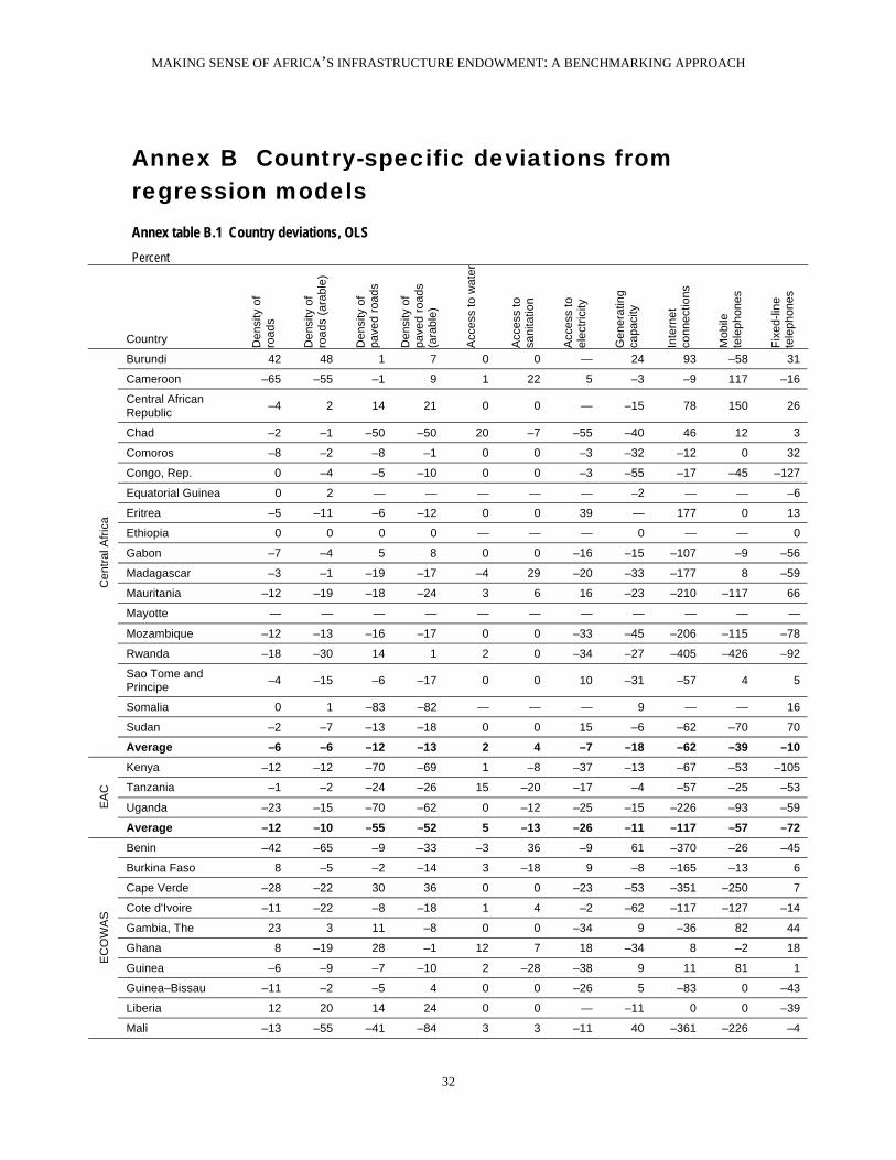
MAKING SENSE OF AFRICA’S INFRASTRUCTURE ENDOWMENT: A BENCHMARKING APPROACH
32
Annex B Country-specific deviations from
regression models
Annex table B.1 Country deviations, OLS
Percent
Country De
nsity o
f ro
ad
s
De
nsity o
f ro
ad
s (
ara
ble
)
De
nsity o
f p
ave
d r
oa
ds
De
nsity o
f p
ave
d r
oa
ds
(ara
ble
)
Acce
ss t
o w
ate
r
Acce
ss t
o
sa
nita
tio
n
Acce
ss t
o
ele
ctr
icity
Ge
ne
ratin
g
ca
pa
city
Inte
rne
t co
nn
ectio
ns
Mo
bile
te
lep
ho
ne
s
Fix
ed
-lin
e
tele
ph
on
es
Burundi 42 48 1 7 0 0 — 24 93 –58 31
Cameroon –65 –55 –1 9 1 22 5 –3 –9 117 –16
Central African Republic
–4 2 14 21 0 0 — –15 78 150 26
Chad –2 –1 –50 –50 20 –7 –55 –40 46 12 3
Comoros –8 –2 –8 –1 0 0 –3 –32 –12 0 32
Congo, Rep. 0 –4 –5 –10 0 0 –3 –55 –17 –45 –127
Equatorial Guinea 0 2 — — — — — –2 — — –6
Eritrea –5 –11 –6 –12 0 0 39 — 177 0 13
Ethiopia 0 0 0 0 — — — 0 — — 0
Gabon –7 –4 5 8 0 0 –16 –15 –107 –9 –56
Madagascar –3 –1 –19 –17 –4 29 –20 –33 –177 8 –59
Mauritania –12 –19 –18 –24 3 6 16 –23 –210 –117 66
Mayotte — — — — — — — — — — —
Mozambique –12 –13 –16 –17 0 0 –33 –45 –206 –115 –78
Rwanda –18 –30 14 1 2 0 –34 –27 –405 –426 –92
Sao Tome and Principe
–4 –15 –6 –17 0 0 10 –31 –57 4 5
Somalia 0 1 –83 –82 — — — 9 — — 16
Sudan –2 –7 –13 –18 0 0 15 –6 –62 –70 70
Ce
ntr
al A
fric
a
Average –6 –6 –12 –13 2 4 –7 –18 –62 –39 –10
Kenya –12 –12 –70 –69 1 –8 –37 –13 –67 –53 –105
Tanzania –1 –2 –24 –26 15 –20 –17 –4 –57 –25 –53
Uganda –23 –15 –70 –62 0 –12 –25 –15 –226 –93 –59 EA
C
Average –12 –10 –55 –52 5 –13 –26 –11 –117 –57 –72
Benin –42 –65 –9 –33 –3 36 –9 61 –370 –26 –45
Burkina Faso 8 –5 –2 –14 3 –18 9 –8 –165 –13 6
Cape Verde –28 –22 30 36 0 0 –23 –53 –351 –250 7
Cote d'Ivoire –11 –22 –8 –18 1 4 –2 –62 –117 –127 –14
Gambia, The 23 3 11 –8 0 0 –34 9 –36 82 44
Ghana 8 –19 28 –1 12 7 18 –34 8 –2 18
Guinea –6 –9 –7 –10 2 –28 –38 9 11 81 1
Guinea–Bissau –11 –2 –5 4 0 0 –26 5 –83 0 –43
Liberia 12 20 14 24 0 0 — –11 0 0 –39
EC
OW
AS
Mali –13 –55 –41 –84 3 3 –11 40 –361 –226 –4
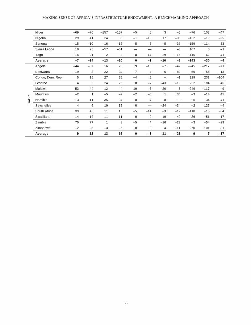
MAKING SENSE OF AFRICA’S INFRASTRUCTURE ENDOWMENT: A BENCHMARKING APPROACH
33
Niger –69 –70 –157 –157 –5 6 3 –5 –76 103 –47
Nigeria 29 41 24 36 –1 –18 17 –35 –132 –19 –25
Senegal –15 –10 –16 –12 –5 8 –5 –37 –159 –114 33
Sierra Leone 19 25 –57 –51 — — — –3 107 0 –1
Togo –14 –21 –2 –8 –8 –14 –29 –16 –415 62 41
Average –7 –14 –13 –20 0 –1 –10 –9 –143 –30 –4
Angola –44 –37 16 23 9 –10 –7 –42 –245 –217 –71
Botswana –19 –8 22 34 –7 –4 –6 –82 –56 –54 –13
Congo, Dem. Rep. 5 15 27 36 –4 5 – –1 329 231 –104
Lesotho 4 6 24 26 0 –7 –43 –16 222 184 46
Malawi 53 44 12 4 10 8 –20 6 –249 –117 –9
Mauritius –2 1 –5 –2 –2 –6 1 35 –3 –14 45
Namibia 13 11 35 34 8 –7 8 — –6 –34 –41
Seychelles 4 6 10 12 0 — –24 –34 –2 127 –4
South Africa 39 45 11 16 –5 –14 –3 –12 –110 –18 –34
Swaziland –14 –12 11 11 0 0 –19 –42 –36 –51 –17
Zambia 70 77 1 8 –5 4 –16 –29 –3 –54 –29
Zimbabwe –2 –5 –3 –5 0 0 4 –11 270 101 31
SA
DC
Average 9 12 13 16 0 –3 –11 –21 9 7 –17

MAKING SENSE OF AFRICA’S INFRASTRUCTURE ENDOWMENT: A BENCHMARKING APPROACH
34
Annex table B.2 Country deviations, instrumental variables
Percent
Country De
nsity o
f ro
ad
s
De
nsity o
f ro
ad
s (
ara
ble
)
De
nsity o
f p
ave
d r
oa
ds
De
nsity o
f p
ave
d r
oa
ds
(ara
ble
)
Acce
ss t
o w
ate
r
Acce
ss t
o
sa
nita
tio
n
Acce
ss t
o
ele
ctr
icity
Ge
ne
ratin
g
ca
pa
city
Inte
rne
t co
nn
ectio
ns
Mo
bile
te
lep
ho
ne
s
Fix
ed
-lin
e
tele
ph
on
es
Burundi –72 –472 –82 –117 44 –32 — –80 –100 –100 –130
Cameroon 32 –76 –84 –89 –16 –9 17 –76 –88 –64 –90
Central Afr. Rep. 84 –22 –98 –89 –17 –46 –44 –94 –99 –99 –93
Chad 123 6 –99 –104 –46 –85 –80 –98 –96 –97 –96
Comoros –60 –8 70 — 33 –69 — –82 –108 –102 69
Congo, Rep. 94 92 –63 –38 –50 –80 –89 –90 –94 –67 –96
Equatorial Guinea 13 36 — — — — — –80 — — –72
Eritrea 85 16 –80 –139 –17 –83 –84 –100 –220 –61 –35
Ethiopia 64 –348 –95 –107 — — — –91 — — –138
Gabon 106 –49 –94 –87 –10 –28 –92 –48 –88 –42 –86
Madagascar 31 39 –76 — –34 –37 –63 –88 –93 –88 –90
Mauritania 237 –50 –92 –80 –30 –9 –19 –79 –89 14 –76
Mayotte — — — — — — — — — — —
Mozambique 89 –51 –78 58 –40 –47 –84 –10 –85 –71 –90
Rwanda –66 –408 –82 –114 31 –50 –33 –139 –102 –106 –110
Sao T&P –48 139 129 — 3 –61 — –53 –229 –136 12
Somalia 62 289 –94 –218 — — — –93 — — 403
Sudan 189 –95 –95 –83 –4 –33 –65 –85 –49 –86 –24
Ce
ntr
al A
fric
a
Average 57 –57 –63 –93 –11 –48 –58 –81 –110 –79 –44
Kenya 12 –8 –76 36 –15 –12 –59 –75 68 –33 –74
Tanzania 18 73 –93 128 6 –14 18 –83 –83 –76 –88
Uganda 4 251 –92 –106 –11 –32 –74 –72 –129 — –19 EA
C
Average 11 106 –87 20 –7 –19 –39 –77 –48 –54 –60
Benin 40 –86 –79 –85 –9 –41 –5 –88 130 –60 –68
Burkina Faso 59 –15 –87 –111 –19 –78 –61 –86 –82 –63 –50
Cape Verde –37 –25 159 86 11 –25 — –92 –300 74 81
Cote d'Ivoire –2 –33 –73 –72 11 –28 –34 –78 –81 –59 –79
Gambia, The –68 78 –14 — 13 –12 –46 –86 227 54 –40
Ghana –21 –29 –26 73 10 0 73 –67 –49 –46 –61
Guinea 8 252 –48 –488 –28 –75 –64 –65 314 –84 –92
Guinea–Bissau 6 –1 –80 159 –2 –38 1 –94 –84 –100 –82
Liberia 20 28 –88 –62 –18 –48 — –42 –99 –100 –95
Mali 144 –68 –96 –151 –33 –10 — –84 –94 –85 –85
Niger 173 –48 –98 –105 –30 –77 76 –90 –98 –96 –94
EC
OW
AS
Nigeria –28 –66 –36 –49 –23 –38 3 –77 –151 –23 –87

MAKING SENSE OF AFRICA’S INFRASTRUCTURE ENDOWMENT: A BENCHMARKING APPROACH
35
Senegal 36 –76 –53 –69 –10 0 –35 –87 296 9 –58
Sierra Leone –15 107 –85 65 — — –153 –84 –134 –95 –87
Togo –3 –79 –46 –12 –28 –42 –38 –95 25 –67 –69
Average 21 –4 –50 –59 –11 –37 –24 –81 –12 –49 –64
Angola 83 6 –39 333 –37 –40 –82 –80 –91 –80 –92
Botswana 153 –9 –84 55 8 –21 –79 –84 –85 –42 –59
Congo, Dem. Rep.
37 163 –97 –200 –30 –45 –136 –71 –99 –95 –99
Lesotho –14 24 –41 381 11 –36 –88 –80 –78 –56 –60
Malawi –31 401 –65 –129 9 –25 –66 –73 –84 –79 –32
Mauritius –99 –34 122 64 41 –14 –45 17 –194 –384 152
Namibia 69 359 –79 334 12 –43 –53 –100 –81 –67 –49
Seychelles –91 — 165 — –7 — — –62 –34 –31 –14
South Africa –33 –34 –11 –60 1 21 –23 115 –57 –4 –24
Swaziland –6 –8 –45 56 –19 –20 –79 –73 –87 –78 –59
Zambia 23 –9 –60 –48 –26 –9 –53 26 –41 –77 –80
Zimbabwe –25 66 18 147 20 5 –60 12 18 –75 –37
SA
DC
Average 6 84 –18 85 –1 –20 –69 –38 –76 –89 –38
Source: As for table 2.1.
Note: Deviations larger than 500% or less than –500% have been dropped.

MAKING SENSE OF AFRICA’S INFRASTRUCTURE ENDOWMENT: A BENCHMARKING APPROACH
36
Annex C Regional infrastructure endowment
Infrastructure category
Transport Information and communication
technology Energy
Density of paved
road network
Density of total
road network
Density
of fixed- line
phones
Density
of mobile phones
Density
of Internet connections
Electrical
generating capacity
Access to
electricity
Water Sanitation
km per 1,000 km2, 2001
Region/
country total arable total arable
subscribers per
1,000 people,
2004
subscribers per
100 people,
2004
MW per 1 million people,
2003
% house- holds with
access, 2004
% households with access, 2002
ECOWAS 38 301 144 1,279 28 72 2.4 31 18 63 35
Benin 12 55 60 273 9 — 1.4 18 22 68 32
Burkina Faso 7 48 46 298 6 31 0.4 10 13 51 12
Cape Verde 213 2,047 273 2,625 148 133 5.3 21 20 80 42
Côte d’Ivoire 15 156 156 1,603 — 86 1.8 55 39 84 40
Gambia 85 338 496 1,982 — 118 3.4 21 5 82 53
Ghana 58 326 194 1,088 14 78 1.7 63 54 79 58
Guinea 20 565 124 3,427 — — 5.8 35 5 51 13
Guinea-Bissau 13 117 122 1,138 — — 2.0 13 8 59 34
Liberia 6 149 95 2,410 — — — 98 5 62 26
Mali 1 39 12 319 6 30 0.5 24 8 48 45
Niger 1 18 8 225 2 11 0.2 9 8 46 12
Nigeria 65 208 210 672 8 71 1.4 43 40 60 38
Senegal 22 170 74 579 — 90 4.7 23 30 72 52
Sierra Leone 13 187 158 2,263 — — 0.2 22 5 57 39
Togo 42 91 132 287 — — 4.4 8 9 51 34
EAC 8 93 105 1,286 6 54 2.1 24 7 64 45
Kenya 13 165 110 1,364 9 76 4.6 36 8 62 48
Tanzania 4 87 93 2,060 — 44 0.9 24 11 73 46
Uganda 8 29 113 436 3 42 0.7 12 4 56 41
SADC 92 3,636 214 6,164 74 180 5.5 175 21 71 43
Angola 15 638 41 1,712 — 61 1.2 50 12 50 30
Botswana 10 1,479 18 2,690 77 319 3.3 75 22 95 41
Congo, DR 2 55 67 2,262 — — — 48 7 46 29
Lesotho 36 329 196 1,796 21 88 2.4 45 5 76 37
Malawi 31 132 240 1,024 7 18 0.4 27 5 67 46
Mauritius 956 1,939 980 1,989 287 413 14.6 548 100 100 99
Namibia 10 983 76 7,619 64 142 3.7 — 34 80 30
Seychelles 700 31,532 829 37,337 253 589 24.7 359 30 87 —
South Africa 60 498 297 2,445 — 428 7.9 883 66 87 87
Swaziland — — — — — 101 3.3 118 20 52 52
Zambia 10 141 121 1,716 — 26 2.1 172 12 55 55

MAKING SENSE OF AFRICA’S INFRASTRUCTURE ENDOWMENT: A BENCHMARKING APPROACH
37
Zimbabwe 48 575 252 3,025 25 31 6.3 150 20 83 83
Central Africa 41 416 132 1,790 13 74 1.7 44 18 58 28
Burundi 37 97 520 1,369 — — 0.4 6 5 79 36
Cameroon 9 70 72 564 — 96 1.0 56 49 63 48
Cen. Afr. Rep. 1 34 38 1,233 3 15 0.2 10 5 75 27
Chad 0.2 7 26 910 1 13 0.7 3 3 34 8
Comoros 302 841 395 1,099 — — 1.0 17 20 94 23
Congo, Rep. 4 670 37 6,905 4 99 0.9 32 21 46 9
Eq. Guinea — — 103 2,218 — 113 1.0 20 20 44 53
Eritrea 7 150 34 689 9 5 1.2 — 17 57 9
Ethiopia 4 33 29 268 — 3 0.2 10 13 22 6
Gabon 3 248 32 2,510 28 359 3.0 305 31 87 36
Madagascar 10 194 89 1,755 — 18 0.5 17 8 45 33
Mauritania 2 177 7 1,569 — 175 0.5 42 50 56 42
Mozambique 7 139 38 744 — 36 0.7 125 7 42 27
Rwanda 38 94 456 1,125 3 16 0.4 5 5 73 41
San Tome and
Principe 227 3,633 333 5,333 — — 12.2 64 20 79 24
Somalia 4 245 35 2,075 25 63 1.7 8 3 29 25
Sudan 2 25 5 70 29 30 3.3 23 30 69 34
— = data not available.