manual gid
DESCRIPTION
Element finitTRANSCRIPT

INTRODUCTION
1
1.1 What's GiD
GiD is an interactive graphical user interface used for the definition, preparation and visualization of all the data related to a numerical simulation. This data includes the definition of the geometry, materials, conditions, solution information and other parameters. The program can generate a mesh suitable for several numerical methods (finite element, finite volume or finite difference, particle based or meshless methods) and write the information for a numerical simulation program in its required format. It is also possible to run these numerical simulations from within GiD and then visualize the results of the analysis.
GiD can be customized and configured by users so that the data required for their own solver modules may be generated. These solver modules may then be included within the GiD software system.
The program works, when defining the geometry, in a similar way to a CAD (Computer Aided Design) system. One characteristic is that the geometry is constructed in a hierarchical mode. This means that an entity of higher level (dimension) is constructed over entities of lower level; two adjacent entities will then share the same lower level entity.
All materials, conditions and solution parameters can be defined on the geometry itself, separately from the mesh as the meshing is only done once the problem has been fully defined. The advantages of this are that, using associative data structures, modifications to the geometry can be made and all other information will automatically be updated and ready for the analysis run. All this information can also be linked to Groups instead of geometry, so as all the entities (geometry and mesh) included in the group inherit it.
Advanced visualization tools (stereoscopic view, use of shadows, mirror effect, etc...) are used in order to provide the user with the best view of the model in order to get a better understanding of the 3D geometry of the model and the results of the simulation. Furthermore, snapshots or animations of the model using any visualization mode and including results can be exported in several formats with the desired resolution.
Full graphic visualization of the geometry, mesh and conditions is available for comprehensive checking of the model before the analysis run is started. More comprehensive graphic visualization features are provided to evaluate the solution results after the analysis run. This postprocessing user interface can also be customized depending on the analysis type and the results provided.
1.2 GiD Manuals

2 Reference Manual
The whole GiD manual is splitted in 3 volumes: Reference, User and Customization manuals.
In this volume, Reference Manual, there is a first part devoted to general aspects, which provides information on the basic aspects of the program. In this way, you can gain confidence and become more familiar with the system in order to take advantage of all the available facilities.
Then you can find detailed information of all the features of GiD following the structure of the menus (both in preprocessing and postprocessing part of GiD).
The User Manual volume contains a collection of tutorials and practical information for learning the basics and advanced features of GiD, covering full flow of GiD user from preprocessing to postprocessing going trough meshing, analysis and introduction to customization.
The last volume, Customization Manual, its adressed basically to developers of modules, and explains how to customize your files so that you can introduce and run different solver modules from GiD according to your own requirements. The way of customizeing graphical interface and behaviour of GiD as users needs is also explained in this manual.
Different kinds of fonts are used to help you follow all the possibilities offered by the code:
1 font is used for the options found in the menus and windows and for literal code.2 font is used for special references in some parts.

GENERAL ASPECTS
3
2.1 GiD Basics
GiD is a geometrical system in the sense that, having defined the geometry, all the attributes and conditions (i.e. material assignments, loading, conditions, etc.) are applied to the geometry without any reference to a mesh. Only when everything has been defined is the meshing of the geometrical domain carried out. This methodology facilitates alterations to the geometry while maintaining the definitions of the attributes and conditions. Alterations to the attributes or conditions can be made simultaneously without needing to reassign the geometry. New meshes can also be generated if necessary and all the information will automatically be assigned correctly.
GiD also provides the option of defining attributes and conditions directly to the mesh once it has been generated. However, if the mesh is regenerated, it is not possible to maintain these definitions and therefore all attributes and conditions must then be redefined.
In general, the entire workflow for a numerical simulation can be defined as:
1 Define the geometry of the domain: it can be done by generating the geometry using GiD or importing it from another CAD software.
2 Define attributes and conditions and assign it onto the geometrical model (both meshing properties and data needed for the solver).
3 Generate the mesh.4 Carry out the simulation.5 Visualize the results.
Depending upon the results in step (3), it may be necessary to return to the previous steps to make alterations and re-run the simulation.
Building a geometrical domain in GiD is based on four levels of geometrical entity: points, lines, surfaces and volumes. Entities of higher level are constructed over entities of lower level; two adjacent entities can therefore share the same level entity. Here are a few examples:
Example 1: One line has two lower level entities (points), each of them at an extreme of the line. If two lines are sharing one extreme, they are really sharing the same point, which is a unique entity.
Example 2: When creating a new line, what is really being created is a line plus two points or a line with existing points created previously.
Example 3: When creating a volume, it is created over a set of existing surfaces, which are joined to each other by common lines. The lines are, in turn, joined to each other by common points.

4 Reference Manual
All domains are considered in 3-dimensional space but if there is no variation in the third coordinate (into the screen) the geometry is assumed to be 2-dimensional for the purposes of analysis and the visualization of results. Thus, to build a geometry with GiD, the user must first define the points, join these together to form lines, create closed surfaces from the lines and define closed volumes for the surfaces. Many other facilities are provided for creating the geometrical domain; these include: copying, moving points, automatic surface creation, etc.
The geometrical domain can be created in a series of layers where each one is a separate part of the geometry. Any geometrical entity (points, lines, surfaces or volumes) can belong to a particular layer. It is then possible to view and manipulate some layers and not others. The main purpose of these layers is to offer a visualization and selection tool as they are not used in the analysis. An example of the use of layers might be a chair where the four legs, seat, backrest and side arms are the different layers.
With GiD you can import a geometry or mesh created with an external CAD program.
The geometry formats supported at present are: IGES, STEP, Parasolid, ACIS , VDA, DXF, KML (Google Earth), Shapefile and Rhinoceros file formats together with several cartographical and topographical formats.
Mesh data can be read in NASTRAN, STL, VRML, 3DStudio, CGNS, VTK and other formats
Attributes and conditions are applied to the geometrical entities (points, lines, surfaces and volumes) using data input dialog boxes. These menus are specific to the particular solver that will be employed for the simulation and, therefore, the solver needs to be defined before attributes are defined. The form of these menus can also be configured for the user's own solver module, as is explained below and later in this manual.
Once the geometry and attributes have been defined, a mesh can be generated using the mesh generation tools supplied within the system. User can generate the mesh with the defualt parameters, or can set specific meshing properties or tune some parameters in order to get the desired final mesh. Structured, semi-structured, unstructured and cartesian meshes can be generated, containing triangular,quadrilateral or circle elements for surface meshes and tetrahedral, hexahedral, prism or sphere elements for volume meshes. Different kinds of quadratic type can be generated for each element type. The automatic mesh generation facility uses a background mesh concept for which the user is required to supply a minimum number of parameters.
Simulations are carried out from within GiD by using the calculate menu. Indeed, specific solvers require specific data that must have been prepared previously. A number of solvers may be incorporated together with the correct preprocessing interfaces.
The final stage of graphic visualization is flexible in order to allow the user to critically evaluate the results quickly and easily. The menu items are generally determined by the results supplied by the solver module. This not only reduces the amount of information

5GiD Basics
stored but also allows a certain degree of user customization.
One of the major strengths of GiD is that the user can define and configure his own graphic user interface within GiD. The first step is to create some configuration files which define new windows, where the final user will enter data, such as materials or conditions. The format that GiD uses to write a file containing the necessary data in order to run the numerical simulation program must also be defined in a similar way. This preprocessor or data input interface will thus be tailored specifically to the user's simulation program, but employing the facilities and functionality of the GiD system. The second step is to include the user's simulation program within GiD so that it may be run utilizing the calculate menu option. The third step consists of writing an interface program, or using the 'gidpost' library, which provides the results information in the format required by the GiD graphic visualizer, thereby configuring the postprocessing menus. This post-analysis interface may be included fully in the GiD system so that it runs automatically once the simulation run has terminated.
Details on this configuration can be found in later chapters.
2.2 Invoking GiD
When installing GiD on Windows, the useful way is to start GiD from desktop icon:
There is also added a direct access from the programs list of the start menu.
The first time that you execute GiD, the following window will be displayed.

6 Reference Manual
Where you can choose OpenGL working mode and GiD theme.
This options can be found inside GiD in Utilities -> Preferences window
Also it's possible to change OpenGL options by clicking on / in the bottom right corner of GiD window
On Start menu you can also found an special option, 'GiD Safe Mode', then a window will be open to ask the user to select how to handle OpenGL graphics: by software or by hardware (some graphic cards and drivers have problems with the hardware option, the screen can show corrupted images or even GiD can crash)

7Invoking GiD
When starting the GiD program from a shell or script it is possible to supply several options in the same command line.
With
gid -help
the program will list the possible command line options.
Command line syntax:
gid [-b[{+/-}g][{+/-}i][{+/-}w] batchfile] [-t tcl_command] [-h] [-p problem] [-e cmd] [-n] [-n2] [-c][-c2] [filename]
All options and filename are optional. filename is the name of a problem to be opened (the .gid extension is optional).
Options are:
-b batchfile executes batch_file as a script file (see Batch file -pag. 45- ). +/- g Enable/Disable Graphics (if -g, GiD does not redraw until the batch file has finished). +/- i Enable/Disable GraphInput (enable or disable peripherals while the batch file is being executed: mouse, keyboard, etc.). +/- w Enable/Disable Windows (GiD displays - or does not display - windows which require interaction with the user). -h shows GiD's command line arguments. -t tcl_command to evaluate tcl code just after read the filename if it has been specified
example:
gid -t "WarnWinText [GiD_Info Project]" C:\temp\myexample
-p problem loads problem as the type of the problem to be used for a new project. -e cmd can continue until the end of the line. It executes anything as if it were a group of commands entered into GiD. -n runs the program without any window. It is most useful when used with the option batchfile. Tcl is loaded but not Tk and most GiD scripts. -n2 runs the program with minimized window, the Tk library and GiD scripts are loaded. This option is useful if you use Tcl and maybe Tk commands in a batch file. -c inifile to read preferences from an alternative user configuration file, instead the default 'gid.ini' (e.g. to run batch tests with preference values specified in a file).-c2 inifile to read/write with an alternative user configuration file, instead the default 'gid.ini' (e.g. to store separatelly preferences of problemtype or GiD version)
The difference between -c and -c2 is that -c only read the configuration file, but not try to write it with current values when exit GiD.

8 Reference Manual
-openglconfig (Only for Windows ): this allows you to choose between the accelerated OpenGL, if present, or the generic implementation, if you experience troubles using the accelerated libraries of the graphics card.
Note: by default, when running a batch file from the command line or importing a Batch file -pag. 45- from the 'Files->Import' menu, graphics are disabled, and then for example is not possible to save an snapshot in a file. To enable graphic features use gid -b+g batchfile
On the other hand when reading a file with the Read batch window -pag. 104- graphics are enabled.
Other useful options are:
gid -compress [ -123456789ad] file_name_in file_name_out
in order to compress (gzip) a file, e.g. to compress '.dat' files or new postprocess formatted data files.
And:
gid [ -PostBinaryFormat { 1.0 / 1.1}] -PostResultsToBinary file_in file_out
in order to transform ASCII results files into compressed binary ones. You can select whether to use the binary format 1.0 or 1.1. The default format (recommended) is 1.1.
gid -tclsh ?<tcl_filename>?
To source a file in a tclsh or open an interactive Tkcon console, replacing the use of tclsh.exe
OFFSCREEN mode:
Since GiD version 10.1.3b there is a new executable called 'gid_Mesa' which, together with the above described options, also has two new options:
-offscreen [ WIDTHxHEIGHT] --> to launch GiD in OffScreen mode ( with no graphic window)
--> using an in memory framebuffer of WIDTH x HEIGHT pixels ( by default 960x640)
--> This option is usefull to launch GiD in batch mode ( in background) to create images and animations without any graphic feedback, for instance to create very large animation using a batch queue on a remote computer or in background.
-output file_name -> Writes GiD's stdout into $file_name file.
2.2.1 Settings

9Settings
GENERIC SETTINGS
\plugins folder
It is possible to extend GiD with new features implemented in Tcl scripting language, by adding this .tcl files to the folder \plugins of GiD
All Tcl files inside this folder will be automatically sourced when starting GiD.
It is hightly unrecommended to modify or add any script to the \scripts GiD folder, because this changes will be lost when installing new versions.
\templates folder
All .bas files of this folder will be showed in the Files->Export->Using template .bas (only mesh) menu
This .bas templates are text files with a syntax explained in the Template File from Customization Manual section, used to export GiD data of mesh (and maybe other attached data).
dump.bas is an example template that write in a simple way most of the GiD mesh and attached data information.
\problemtypes folder
This folder must contain customizations of GiD to handle external third part solvers (see Customization Manual)
USER SETTINGS
Each user has its own copy of some GiD settings (like preferences variables, or window sizes).
This information is saved in a file named 'gid.ini' that is stored in a different place depending on the platform
e.g.
Windows XP: C:\Documents and Settings\<current user>\Application Data\GiD\gid.ini
Windows Vista / Windows 7 / Windows 8: C:\Users\<current user>\AppData\Roaming\GiD\gid.ini
Linux / Mac OS X: $(HOME)/.gidDefaults
And by default some folders like "Application Data" are hidden.
This settings are automatically saved when exiting GiD, and loaded when starting.
2.3 User Interface

10 Reference Manual
The user interface allows you to interact with the program. It is composed of buttons, windows, icons, menus, text entries and the graphical output of certain information. You can configure the interface to display things in a certain way, and may use as many menus and windows as required.
The initial layout of GiD is consists of a large graphical area with pull-down menus at the top, a command line at the bottom, a message window above it and an icon bar. The project that is being run is displayed in the window title bar. The pull-down and 'click on' menus are used to access GiD commands quickly. Some of them offer a shortcut for easier access - these are activated by holding the Ctrl key and pressing the appropriate letter key(s).
Right-clicking the mouse while the cursor is over the graphical area opens an on-screen menu with some visualization options. To select one of them, right- or left-click on the option; to quit, left-click anywhere outside the menu.
The first option in this menu is called Contextual . It will give different options depending on the function currently being used.
The pair of icon bars contain some facilities that also appear in the graphical area of the window or in the menu bar. When left-clicking on the icon, the corresponding command is performed or an icon menu with several options will be shown. When right-clicking (or using the center button if there is one), a menu with the options help and configure toolbars will appear allowing you to get a description of the icon or to configure the position of the toolbars. The description also appears when the cursor remains over the icon for a couple of seconds.

11User Interface
To configure the position and view of the toolbars, the Toolbars position window can be called from Utilities -> Tools -> Toolbars, or by right-clicking over a toolbar.
Toolbars window
2.3.1 Top menu
The Top Menu offers various types of commands.
It is important to note that these options will differ depending on the whether the user is performing a preprocessing or postprocessing analysis, and that the options needed in each case differ as well.
Two possible configurations of the Top Menu are presented below:
In the preprocessing phase:
And in the postprocessing phase:
The menus "Files", "View" and "Utilities" can be found on both modes, therefore the description of these menus can be found under "GENERAL ASPECTS" chapter of this

12 Reference Manual
Manual.
2.3.2 Toolbars
The Standard bar has common options for both pre- and postprocessing components, including: open, take a snapshot, print, preferences, help, exit and others.
Standard toolbar in preprocess
Standard toolbar in postprocess
The different icons represent, from left to right:
New: PRE: the existing project is closed and a new one is created. POST: the model is closed.Open: PRE: closes the current project and opens an existant one. POST: closes the current model and reads an existant mesh with its results.(only in postprocess) Open multiple: Open multiple postprocess files.Save: PRE: saves de project. POST: saves de postprocess information in a new binary file.
----
Previous view, Next view: no navigate through the used views.List of views: shows a list of some predefined and user-saved views.Fullscreen: Change to fullscreen mode.Fast draw mode: Enable/disable fast draw mode
----
Take a snapshot: takes a picture of the current visualization, using the Page and capture settings -pag. 56- options.Print: print using the the Page and capture settings -pag. 56- options.
----
Toggle between preprocess and postprocess.Copy: PRE: shows the copy window, POST: shows the transformation window.(only in preprocess)Layers Combobox: Combobox to select layer in use.Layers/Meshes/Sets: PRE: pops-up the 'Layer' window, POST: pops-up the 'View Style' window.(only in postprocess) pops-up result, graphs or animation windows respectively.(only in postprocess) Animations Controls.
----
Preferences: pops-up the preferences window to select general, meshing, graphical, fonts options, among others.

13Toolbars
Help: shows GiD's help.----
Exit: quits the program.GiD icon that show also our current passwort type: blue=profesional, red=evaluation, half blue and half red=conection fault short time period of profesional version before change to evaluation.
The Geometry & view bar has some of the view options common to pre- and postprocessing, such as zooming, panning, rotating, etc. But certain icons are specific to preprocessing and others to postprocessing.
Geometry & View bar in preprocess
The different icons represent, from left to right:
Zoom in: zooms the project inZoom out: zooms the project outZoom frame: adjust the visualization to comprise the whole modelRedraw: redraws the model, useful if the graphical window gets 'dirty'Rotate trackball: rotates de model dynamically using the mouse as 'spaceball'Pan dynamic: translates the model dinamycally
----
Create lineCreate arcCreate NURBS lineCreate polyline
----
Create NURBS surfaceCreate volumeCreate object
Left-click on Create object, GiD opens another window to choose from rectangle, polygon, circle, sphere, cylinder, cone, prism or torus
----
Delete: to delete geometric entitiesLeft-click on Delete, GiD opens another window with the different entities to be deleted: Point, Line, Surface, Volume or All types.
List entities: shows information of the selected entitiesLeft-click on List entities, GiD opens another window with the different entities able to be listed: Points, Lines, Surfaces or Volumes.

14 Reference Manual
----
Toggle between geometry view and mesh view
Note: The position of the icons depends on how the window is positioned.
Geomety & View bar in postprocess
On the postprocess toolbar, the first six commands are the same as on the preprocess toolbar, i.e. from Zoom in to Pan.
The remaining icons represent, from left to right:
Change Light Vector: allows you to change the light direction (see Render -pag. 62- ).Display style: when you click here, a menu appears with each icon corresponding to a display option: Boundaries, Hidden Boundaries, All Lines, Hidden Lines, Body, Body Boundaries, Body Lines, points or BoundaryPoints.Culling: allows you to switch on or switch off the front faces and/or the back faces.
----
Mesh selection: select the volumes to switch them on or off.Set selection: select the surface sets to switch them on or off.Cut selection: select the cuts to switch them on or off.
----
Cut meshes/sets: cut the volume or surface meshes.----
Set maximum value: set a maximum value for contour fills.Set minimum value: set a minimum value for contour fills.Contour Options: Choose between Logarithmic scale, scale result by multiplier factor ,scale result by adderfactor and Reset limit values.List nodes and elements information: list information (conectiviti, set number, results, etc.) about selected nodes or elements.
Notes:
If windows are used to enter the data, it is generally necessary to accept this data before closing the window. If this is not done, the data will not be changed.
Usually, commands and operations are invoked by using the menus or mouse, but all the information can be typed into the command line.

15Toolbars
The Macros bar allows the creation and execution of macros defined by the user or predefined by GiD:
Default Macro preprocessing
Default Macro posprocessing
Record macro / stop recording macro: stars a new macro and registers each operation in GiD until stop is pressed.Edit macros...: a window will pop-up allowing the user to edit the macro, rename it or change its icon and accelerator keys.
---
All other icons are configured from Edit macros window
The View results bar allow the user a quick view of the results:
View result bar
No result: cleans all the results visualizations (contour fill, deformation, vectors, etc. except the graphs), leaving the mesh alone.Togle mesh and graphs view: switches between the graphs visualization and the results visualization mode.
----
Default analysis/step: allows the set the default analysis and step. Used to create the menus with the result's names of the results present on the selected step and analysis.
----
Contour Fill: draws a Contour Fill of the selected result.Contour info: Enable or disable showing the contour fill range under the cursor. Contour Lines: draws the Contour Lines of the selected result.Show min max: shows the maximum and minimum value of the selected result.

16 Reference Manual
Show min: Only shows the minimum.Show max: Only shows the maximum.Show both: Shows minimum and maximum.
Display vectors: draws a vectors of the selected result. This includes vectors, stresses and local axes.Iso surfaces: draws the isosurfaces of the selected result. The user can select the number of isosurfaces and the exact value for each of them.Stream lines: draws stream lines of the selected nodal vector.Result surface: draws a extruded surface acording to the selected result. If the result selected is a vector, uses the vector as extrude direction. If the result selected is a scalar, uses the normal of the noded (which is an average of the normals of the surrounding elements). Deformation: deforms the mesh acording to the selected nodal vector. Graphs: pop-ups a menu with the following options.
Point evolution: displays a graph of the evolution of the selected result along all the steps, of the default analysis, for the selected nodes. Line graph: also called 'section graph' displays a graph defined by the line conectig two selected nodes of the planar XY surface, or of the volume mesh. Point graph: displays a graph of one result against another of the selected results. The option 'all steps' shows the evolution along all steps inside the default analysis, of this result vs. results graph. Border graph: displays a graph of the results on the selected border, using the x, y, z or line distance as abscissa.Integrated graph: Graph of an integrated result over a mesh.Point Complex evolution: Similar to 'Point Evolution' but for complex results, where both real and imaginary part of the result are displayed as 'x' and 'y' in the graph Clear graphs: delete all the created graphs.
2.3.3 Command line
All commands may be entered via the command line (found at the bottom of the GiD window) by typing the full name or only part of it (long enough to avoid confusion with other commands); commands are not case-sensitive. Any function from the Right buttons menu can be used by typing all or part of its name in the command line. Special commands are also available for viewing (zoom, rotation and so on) and these can be typed or used at any time when working from within another function. A list of these special commands is given in View (see View Menu -pag. 58-).
Commands entered by typing are word oriented. This means that the same operation is

17Command line
achieved if one writes the entire command and then presses enter or if one writes a part of it, presses enter and then writes the rest.
All these typed commands can be retrieved using of the up arrow (to recover past commands) and down arrow (to return to more recent commands).
2.3.4 Status and Information
The Status & Information bar located at lower part of GiD's Window, provides basic information at a quick glance.
From left to right you can find:
Zoom factorCurrent number of nodes and elements (Click to acces to Status Window)Current renter mode (Click to change render)Number of layers in Pre, number of sets in Post Mouse coordinates (Click to open "Coordinate window" in Pre and "Change result units" in Post)Current Mode: Pre or Post
2.3.5 Right buttons
Using the Toolbars position window it is possible to enable the Right buttons menu. Only advanced users should use these buttons.
The right buttons menu displays the actual GiD commands that can be entered manually

18 Reference Manual
in the command line and that are actually used to create batch files.
2.3.6 Mouse operations
Mouse's buttons use
As well as selecting the functions to be used, the left mouse button is used to select entities, either individually or picking several within a given area (see Entity selection -pag. 26-), and to enter points in the plane z=0 (see Point definition -pag. 21-).
The middle mouse button is equivalent to escape (see Escape -pag. 29-).
Mouse menu
The right mouse button opens an on-screen menu with some visualization options. To select one of them, use the left or right mouse button; to quit, left-click anywhere outside the menu.
The first option in this menu is called Contextual. You can select from different options relevant to the function currently being used.
Mouse pointer
When the mouse is moved to different windows, depending on the situations, different cursor shapes and colors will appear on the screen.
In some windows a help option will appear when you click the middle or right mouse buttons over an icon.
View control with the mouse
Rotate, pan and zoom are accessible directly from mouse buttons, pressing shift key.
User can access to rotate, pan and zoom view options directly using mouse buttons, while the shift key is pressed:
shift + left mouse button -> ROTATEshift + wheel/center mouse button -> ZOOMshift + right button -> PAN
Note: Mouse wheel always zoom model, also without pressing shift button.
2.3.7 Dark GiD theme
The GUI appearance of GiD can be configured to "Dark GiD theme". This option can be set from Utilities->Preferences and selecting Graphical->Apparence branch.
After restarting GiD, the GUI will appear as follow:

19Dark GiD theme
Dark GiD theme Interface
The Standard bar
Preprocess:
Classic Standard bar
Dark Standard bar
Postprocess:
Classic Standard bar
Dark Standard bar
The Geometry & view bar
Preprocess:
Classic Geometry & View bar

20 Reference Manual
Dark Geometry & View bar
Postprocess:
Classic Geometry & View bar
Dark Geometry & View bar
The Macros bar
Classic Macros bar
Dark Macros bar
The View results bar
Classic View result bar
Classic View result bar
2.4 User Basics
The following features are essential to the effective use of the GiD system. They are, therefore, described apart from the preprocessing facilities section.

21Point definition
2.4.1 Point definition
Many functions inside GiD need points to be defined by the user. Points are the lowest level of geometrical entity and therefore the most commonly used. Consequently, it is important that you have a thorough understanding of how to do this. Sometimes an existing point is required and sometimes a new point must be defined.
Window for entering coordinates
All the options explained in this section are available through the window shown above (see Coordinates window (only Preprocessing) -pag. 103-). This window is accessed via the pull-down menu Utilities -> Tools. Here you can choose not only the kind of reference system - cartesian, cylindrical or spherical - but also whether to use a global or local coordinate system and whether the origin of coordinates is fixed or relative (where new coordinates are relative to the last origin point entered).
In general you can enter points in the following ways:
1 Picking in the graphical window.Default: picking a new location in the z=0 plane.Point in line: picking a point on a line.Point in surface: picking a point on a surface.Tangent in line: to get a unitary tangent vector sampled on a point of a curve.Normal in surface: to get a unitary normal vector sampled on a point of a surface.Arc center: to get the coordinates of the center of an arc or a NURBS with this shape, the arc must be selected.Line parameter: to get a point on a line specifying the line and the value of the t parameter from 0 to 1.Surface parameter: to get a point on a parametric surface specifying the surface and

22 Reference Manual
the values of the u and v parameters from 0 to 1.2 Entering points by coordinates.
The x,y,z coordinates must be written in the command line sepating them by comma or spaces (but not both). If z is omited it is assumed as z=0.0
3 Selecting an existing point.Join: change the creation mode from expecting the x,y,z coordinates of a new point to expect the id of an existent point. The point can be specified picked on the screen or entering its id integer number in the command line.
4 Using the Base button.Base: allow pick other point and the command line is filled with its x,y,z coordinates, that could be edited to set the wanted location.
2.4.1.1 Picking in the graphical window
Points are picked in the graphical window in the plane z=0 according to the coordinates viewed in the window. Depending on the activated preferences (see Preferences -pag. 77-), if you select a region located in the vicinity of an existing point, GiD asks whether it should create a new point or use the existing one.
2.4.1.2 Entering points by coordinates
GiD offers a window for entering points in order to create geometries easily, defining fixed or relative coordinates as well as different reference systems - cartesian, cylindrical or spherical.
The coordinates of a point can be entered either in the enter points window or in the command line by following one of two possible formats:
1 The format: x,y,z2 The format: x y z
Coordinate z can be omitted in both cases.
The following are valid examples of point definitions:
5.2,1.0 5.2,18 9 2 8 9,2
All of a point's coordinates can be entered as local or global and through different reference systems in addition to the cartesian one.
1 Local/global coordinates2 Cylindrical coordinates

23Entering points by coordinates
3 Spherical coordinates
2.4.1.2.1 Local-global coordinates
Local coordinates are always considered relative to the last point that was used, created or selected. The Utilities -> Id command allows you to make a reference to one point (see Id -pag. 123- ). Then, to define points using local coordinates referring to the same point, use Options and Fixed Relative when entering each point. The last point selected or created before using this will be the origin of the local coordinate system. It is also possible to enter this central point by its coordinates.
The following are valid examples of defining points using local coordinates:
Example (1):
1,0,0 @2,1,0 (actual coordinates 3,1,0) @0,3,0 (actual coordinates 3,4,0) 2,2,2 @1,0,3 (actual coordinates 3,2,5)
Example (2):
1,0,0 Fixed Relative (when creating the point) @2,1,0 (actual coordinates 3,1,0) @0,3,0 (actual coordinates 1,3,0) 2,2,2 @1,0,3 (actual coordinates 2,0,3)
Example (3):
'local_axes_name'2.3,-4.5,0.0
The last example shows how to enter a point from a local coordinate system called 'local_axes_name' (any name inside the quotation marks will work), previously defined via the option define local axes (see Local axes -pag. 167- ).
All the examples have been presented using a cartesian notation. However, cylindrical or spherical coordinates can also be used.
2.4.1.2.2 Cylindrical coordinates

24 Reference Manual
Cylindrical coordinates can be entered as: r<angle,z
The z_coordinate may be omitted and angles are defined in degrees. Cylindrical coordinates can be applied to global and local coordinate systems.
The following are valid examples of the same point definitions:
example (1):
1,0,0 1.931852<15
example (2):
1,0,0 @1.0<30
2.4.1.2.3 Spherical coordinates
Spherical coordinates can be entered as r<anglexy<anglez
Anglez may be omitted and angles are defined in degrees. Spherical coordinates can be applied to global and local coordinate systems.
The following are valid examples of the same point definitions:
Example (1):
1,0,0 1.73205<18.43495<24.09484
Example (2):
1,0,0 @1.0<45<45
2.4.1.3 Base
Mouse menu: Contextual->Base
If the Base button is selected (it is set by default to No Base), a point can be retrieved from any of the other modes. Then, the coordinates of this point, instead of being used immediately, are written in the command line and can be edited before they are confirmed.

25Base
It is possible to change the way that GiD works with points by default via preferences (see Preferences -pag. 77-).
2.4.1.4 Selecting an existing point
Mouse menu: Contextual->Join Ctrl-a
When using a function that asks for a point, e.g. line creation, GiD will expect you either to enter a new point (the cursor is a cross) or select an existing one (the cursor is a box). To change from the first mode to the second, click the Join button in the Right buttons menu or the Contextual mouse menu, or use the shortcut (Ctrl-a); the option will then change to No Join. Simply select an existing point to pick it. (Ctrl-a) switches from Join to No Join and vice versa.
Note: Be aware not use capital letter (Ctrl-A) will not work.
The special options FJoin and FNoJoin force GiD to change either to Join mode or No Join mode independently of the previous mode.
2.4.1.5 Point in line
Mouse menu: Contextual->Point in line
With this option selected, when creating a new point or line, etc., you can only select points that lie on existing lines. To switch it off, simply select No Point in line.
2.4.1.6 Point in surface
Mouse menu: Contextual->Point in surface
With this option selected, when creating a new point or line, etc., you can only select points that lie on existing surfaces. To switch it off, simply select No Point in surface.
2.4.1.7 Tangent in line
Mouse menu: Contextual->Tangent in line
Using this option, you can pick over a line in the graphical window. A vector will be returned that is the tangent to the line at the point you have picked.
2.4.1.8 Normal in surface
Mouse menu: Contextual->Normal in surface

26 Reference Manual
Using this option, you can pick over a surface in the graphical window. A vector will be returned that is the normal to the surface at the point you have picked.
2.4.1.9 Arc center
Mouse menu: Contextual->Arc center
Using this option, you can left-click on an arc in the graphical window and a point will be created at its center.
2.4.1.10 Grid
Toolbar:
It is possible to use an auxiliary grid of lines to define 2D points easily. The 'snap' function can be activated to force points to grid intersections.
From the preferences window (see Preferences -pag. 77-) it is possible to set the separation between lines and to show the origin, extents, etc. of the coordinates.
There is a small button in the bottom right-hand corner that activates or deactivates the grid and 'snap' functions.
2.4.2 Entity selection
Many commands need to be supplied with entities before they can be applied and the method of selection is always the same. Before selecting entities, you are prompted to decide whether to select points, lines, surfaces or volumes (in some cases this decision is obvious or it is made within the context of the option).
Within one of the generic groups (points, lines, surfaces, volumes, nodes or elements) it does not matter what type of entity is selected (for example, an arc or a spline, both line entities are selected in the same way). After this, if one entity of the desired group is selected, it is colored red to indicate it has been selected and you are prompted to enter more entities. If you select away from any entity, a dynamic box is opened that can be defined by picking again in another place. All entities that are either totally or partly within this box are selected. Once again, you are then prompted to enter more entities.
The normal selection mode is SwapSelection: If one entity is selected a second time, it becomes deselected and its color reverts to normal. In addition there are the options AddToSelection and RemoveFromSel, the former always adding to the selection, the latter always removing entities from the selection.

27Entity selection
Note: Instead of picking a start point and an end point for the selection box, it is possible to press and hold left mouse and move the cursor.
The Clear selection option, which is found in the Contextual mouse menu, deselects all previously selected entities.
It is also possible to select entities by entering their label in the command line. For instance, to select the entity with number 2, input this number, 2, in the command line. To select the entities 3 to 7, input 3:7 in the command line. Entering 3: will select all entities from number 3 to the end and entering :3 will select all options from the beginning to number 3.
If a layer named 'a' exists, it is possible to select all entities belonging to that layer with command: layer:a . Using the command layer: selects all entities not belonging to any layer.
Another way of selecting points or nodes is to write:
plane:a,b,c,d,r
where a,b,c,d and r are real numbers that define a plane and a tolerance in the following way: ax+by+cz+d<r. Points close to that plane are chosen.
When selection lines or surfaces (geometry or mesh) it is possible to pick one or more entities, and use 'ConnectedTangent' to select its connected neighbor entities, if the angle between them is smooth enougth. This is very interesting for example to select coplanar parts.
It is possible select a group on entities that are parents of a single 'lower entity' by using 'ParentsOf', and selecting the lower entity. (e.g. to select all surfaces that are sharing some line)
In some commands, another item is added to the selection group. This item, called AllTypes, means that entities of all levels (points...volumes) will be selected at the same time. In this case, only selection via a dynamic box is possible in the graphical window and all entities (points, lines, surfaces and volumes) in the box are selected.
To finish the entity selection, use escape (see Escape -pag. 29-).
If the Fast Selection option is used, entities are not colored red when selected and choosing an entity twice does not deselect it. This option is available via the Right buttons menu (see Tools -pag. 101-), in Utilities -> Variables.
Caution: Only use Fast Selection when you need to select a large number of entities, for

28 Reference Manual
example in a large mesh, as there is a risk of repeating entities.
Entities belonging to frozen layers (see Layers and groups (only Preprocessing) -pag. 98-) are not taken into account in the selection. Entities belonging to OFF layers cannot be selected directly in the graphical window, but can be selected by giving a number or range of numbers.
It is possible to add filters to the selection so that, after selecting some entities, only the ones satisfying the filter criteria will remain selected. To enter one filter, you must enter the word filter: in the command line followed by one option. The available options are:
HigherEntityMinLengthMaxLengthEntityTypeBadMinAngleBadMaxAngleNumSides
Note: To apply selection filters you can also use the Selection window (see Selection window (only Preprocessing) -pag. 109-).
Note: MinLength and MaxLength can be used either in geometry lines or in elements of the mesh.
Note: NumSides=x can be used for surfaces or volumes, to filter the entities with exactly x number of sides.
For example, the following command:
filter:HigherEntity=1
means that only the entities that have higher entity equal to one will be selected.
Note: A typical use of filter is to select only boundary lines (higher entity=1).

29Escape
2.4.3 Escape
The escape command is used for moving up a level within the Right buttons menus, for finishing most commands, or for finishing selections and other utilities. This command can be applied by:
1 pressing the middle mouse button;2 pressing the ESC key; 3 pressing the escape button in the Right buttons menu;4 writing the reserved word escape in the command line. This is useful in scripts (see
Batch file -pag. 45- ).
All the above options give the same result.
Caution: Escape is a reserved word. It cannot be used in any other context.
2.5 Files Menu
Browser to read and write files and projects
GiD includes the usual ways of saving and reading saved information (Save, Read) as well as other operations, such as importing external files, saving in other formats and so on.
2.5.1 New
Menu: Files->New
Toolbar:
Preprocessing:
Selecting New opens a new project with no title assigned to it.

30 Reference Manual
If a project is currently open and changes have been made since it was last saved, GiD will give the option to save before opening the new project.
PostProcessing:
Clears all postprocess information present in GiD.
2.5.2 Open
Menu: Files->Open
Toolbar:
Preprocessing:
With this command, a project previously saved with Save (see Save (Only Preprocessing) -pag. 32-) or with Save ASCII project (see ASCII project -pag. 51-) can be opened.
Postprocessing:
Reads postprocess information in GiD. If, for instance, the postprocess files are 'PostFile.msh' and 'PostFile.res' and a view file is present with the name 'PostFile.vv' then it will be also read.
For big results files, GiD will use an index file to access the results information faster.
When Reading a file, under the 'Postprocess read options' this index can be rebuild:
The postprocess information can be in ASCII ( Filename.msh and Filename.res), in binary (

31Open
Filename.bin) or a file list ( Several.lst).
The list file can be used to read several postprocess files at once. This includes both mesh, results and graphs files. The list file is just a text file, for a description of it's format please look at the Customization Manual under POSTPROCESS DATA FILES -> List file format.
2.5.3 Open multiple... (Only Postprocessing)
Menu: Files->Open multiple...
Toolbar:
With this option you can load multiple meshes (pairs of .msh and .res, or .bin files) into GiD. This is useful, for instance, when performing an analysis where some or all steps require re-meshing.
From the file browser window, you can select several pairs Project.post.msh and Project.post.res, in one go by left-clicking one file and then <Shift>-left-clicking another so that all the files in between are highlighted; further files can be added or removed individually with <Ctrl>-left-click. Normal operations, such as animation, displaying results and cuts, can be done over these meshes, and they will be actualized when the selected analysis/step is changed, for example by means of View results -> Default analysis/step (see Re-meshing and adaptivity from Customization Manual).
2.5.4 Merge... (Only Postprocessing)
Menu: Files->Merge...
Reads mesh and results information from an ASCII or a binary file and adds them to the current ones. If nodes are already present inside GiD, they will be overwritten. No renumeration is done.
2.5.5 Recent projects and Recent post files
Menu: Files->Recent projects
Menu: Files->Recent post files
You can quickly gain access to files opened recently with GiD.
Recent Post Files: a list of the most recents files read in postprocess is shown, so the user can select them quickier. The number of files can be adjusted by Preferences -pag. 77-.Recent Projects: a list of the most recent GiD projects are shown.

32 Reference Manual
2.5.6 Save (Only Preprocessing)
Menu: Files->Save...
Toolbar:
Using the Save command saves all the information relating to a project - geometry, conditions, materials, mesh, etc. - to the disk.
When a project is saved, GiD creates a directory with the project name and the extension .gid. Files containing all the information are written to this directory. Some of these files are binary and others are ASCII. You can then work with this project directory as if it were a file.
You do not need to write the .gid extension because it will automatically be added to the directory name.
Caution: Be careful if changing some files manually in the Project.gid directory. If done in this way, some information may be corrupted.
Advice: It is recommended to save the project at regular intervals so as not to lose any important information. It is possible to back up files automatically by selecting this option in the Preferences menu (see Preferences -pag. 77-).
2.5.7 Save as... (only Preprocessing)
Menu: Files->Save as...
With this command, GiD allows you to save the current project with another name.
When it is selected, an auxiliary window appears with all the existing projects and directories to facilitate the introduction of the project's new name and directory.
2.5.8 Import
GiD lets you import geometrical models, meshes or results in the following formats.
2.5.8.1 Preprocessing
The file browser could allow some extra "Import options", depending on each case.
Usually these options are hidden, press the arrow icon, if any, to show them
e.g.

33Preprocessing
Most preprocess importations have as extra options the ones related to collapse the model just after be imported:
Automatic collapse after import: To do or not this collapse
Use automatic collapse tolerance: to let the program to get an automatic value of the tolerance, just to join points close that this value.
Tolerance: the user value, in case of not to use the automatic one.
Collapse ignoring layers: the default way: close entities are joined without take into account if they belong to different layers.
2.5.8.1.1 IGES
Menu: Files->Import->IGES...
With this option it is possible to import a file in IGES format (version 5.3); GiD is able to read most of the entities, which are:
Entity number and type (Notes)
100 Circular arc
102 Composite curve
104 Conic arc (ellipse, hyperbola and parabola)
106 Copious data (forms 1, 2, 12 and 63)
108 Plane (form1 bounded)
110 Line
112 Parametric spline curve
114 Parametric spline surface
116 Point
118 Ruled surface

34 Reference Manual
120 Surface of revolution
122 Tabulated cylinder
123 Direction
124 Transformation matrix (form 0)
126 Rational B-spline curve
128 Rational B-spline surface
134 Node
136 Element
140 Offset surface entity
141 Bounded entity
142 Curve on a parametric surface
143 Bounded surface
144 Trimmed surface
184 Solid assembly
186 Manifold solid B-rep object
190 Plane
192 Right circular cylindrical surface
194 Right circular conical surface entity
196 Spherical surface
198 Toroidal surface
308 Subfigure definition
314 Color definition
402 Associativity instance
406 Property entity
408 Singular subfigure instance
502 Vertex
504 Edge
508 Loop
510 Face
514 Shell
The variable ImportTolerance (see Preferences -pag. 77- ) controls the creation of new points when an IGES file is read. Points are therefore defined as unique if they lie further away than this tolerance distance from another already defined point. Curves are considered identical if they have the same points at their extremes and the "mean proportional distance" between them is smaller than the tolerance. Surfaces can also be

35IGES
collapsed.
Entities that are read in and transformed are not necessarily identical to the original entity. For example, surfaces may be transformed into planes, Coons or NURBS surfaces defining their contours and shape.
2.5.8.1.2 STEP
Menu: Files->Import->STEP...
With this option it is possible to read a CAD file in STEP standard format (AP214 Automotive Application protocol only)
2.5.8.1.3 DXF
Menu: Files->Import->DXF...
With this option it is possible to read a file in DXF format (AutoCAD exchange format).
GiD is able to read most of the entities, which are: POINT, LINE, ARC, CIRCLE, ELLIPSE, SPLINE, LWPOLYLINE, MLINE, POLYLINE, VERTEX, TRACE, SOLID, 3DFACE, 3DSOLID, BLOCK, INSERT
A very important parameter to consider is how the points must be joined. This means that points that are close to each other must be converted to a single point. This is done by defining the variable ImportTolerance (see Preferences -pag. 77- ). Points closer together than ImportTolerance will be considered as a single point. Straight lines that share both points are also converted to a single line.
You can use the Collapse function (see Collapse -pag. 154- ) to join more entities.
2.5.8.1.4 Parasolid
Menu: Files->Import->Parasolid...
With this option it is possible to read a file in the Parasolid format (untile version 25001 - ASCII or binary).
The most usual Parasolid file extension is .x_t for ASCII and .x_b for binary format.
The variable ImportTolerance (see Preferences -pag. 77- ) controls the creation of new points when a Parasolid file is read. Points are therefore defined as unique if they lie further away than this tolerance distance from another already defined point. Curves are considered identical if they have the same points at their extremes and the "mean proportional distance" between them is smaller than the tolerance. Surfaces can also be

36 Reference Manual
collapsed.
2.5.8.1.5 ACIS
Menu: Files->Import->ACIS...
With this option it is possible to read a file in ACIS format (version 2000). GiD reads the ASCII version with the SAT Save File Format. ACIS files (in ASCII) have the .sat extension.
2.5.8.1.6 VDA
Menu: Files->Import->VDA...
With this option it is possible to read a file in VDA 2.0 format.
A very important parameter to consider is how the points must be joined. This means that points that are close to each other must be converted to a single point. This is done by defining the variable ImportTolerance (see Preferences -pag. 77- ). Points closer together than ImportTolerance will be considered as a single point. Straight lines that share both points are also converted to a single line.
The Collapse function (see Collapse -pag. 154- ) can be used to join more entities.
2.5.8.1.7 Rhinoceros
Menu: Files->Import->Rhinoceros...
With this option it is possible to read Rhinoceros 5.0 CAD files. This files have the .3dm extension.
2.5.8.1.8 Shapefile
Menu: Files->Import->Shapefile...
With this option it is possible to read a GIS file written in ESRI Shapefile format (version 1000). Shapefiles have the .shp extension.
2.5.8.1.9 XYZ points
Menu: Files->Import->XYZ points...
With this option it is possible to read a set of geometric points. This format is ASCII and consists the coordinates of the points separated with spaces.
Note: If only 2 coordinates are specified, z=0 is assumed.

37XYZ points
If 'Automatic collapse after import' was set, after the import near points will be joined, The variable ImportTolerance (see Preferences -pag. 77- ) controls the joining distance.
The file browser allow some extra "Import options". Usually these options are hidden, press the arrow icon to show them
Collapse: It is possible to set that a collapse must be done after the importation, and its parameters (automatic or specified tolerance). If the collection of points is very big a collapse could be intersting to subsample them, and to avoid very close or repeated coordinates.
Triangulate: If this option is set then a Delaunay triangulation of the points will be done. (this triangulation is made in the xy plane projection)
2.5.8.1.10 KML
Menu: Files->Import->KML...
With this option it is possible to read files with the format KML (of Google Earth).
Extra options:
To projection: KML data is expressed as two dimension coordinates x,y that represents geographic latidude and longitude, it is possible to transform this information to other system:
None: Without any modificationUTM (Universal traverse mercator)MercatorPlateCarree
2.5.8.1.11 NASTRAN mesh
Menu: Files->Import->NASTRAN mesh...
38 Reference Manual
With this option it is possible to read a file in NASTRAN format (version 68), with GiD accepting most of its entities, which are:
Entity name ( Notes)
CBAR CBEAM CROD CCABLE CBUSH CELAS1 CELAS2 CELAS3 RBAR (translated as 2 node bars)
CQUAD4 CQUADR
CHEXA
CTETRA
CPENTA
CTRIA3 CTRIAR
CONM1 CONM2 (translated as 1 node element)
CORD1C CORD1R CORD1S
CORD2C CORD2R CORD2S
GRID
There are two options that can be used when reading a mesh if GiD already contains a mesh:
a Erasing the old mesh (Erase);b Adding the new mesh to the old one without sharing the nodes; the nodes will be
duplicated although they may occupy the same position in the space (AddNotShare).
The properties and materials of elements are currently ignored, because of the difficulties in associating the NASTRAN file properties with the requirements of the analysis programs. Therefore, you have to assign the materials "a posteriori" accordingly. However, in order to make this easier, the elements will be partitioned in different layers, each with the name PIdn, where n is the property identity number associated with the elements as defined in the NASTRAN file. Note that CELAS2 elements do not have associated property identities so these will be created by default when the file is read.
2.5.8.1.12 STL mesh
Menu: Files->Import->STL mesh...
With this option it is possible to read a mesh in STL format. The STL binary format is also supported.
The variable ImportTolerance (see Preferences -pag. 77- ) controls the creation of new points when the file is read.

39VRML mesh
2.5.8.1.13 VRML mesh
Menu: Files->Import->VRML mesh...
With this option it is possible to read a mesh in VRML 2.0 format. The compressed gzip format is also supported.
2.5.8.1.14 3DStudio mesh
Menu: Files->Import->3DStudio mesh...
With this option it is possible to read a mesh in .3ds 3DStudio format.
2.5.8.1.15 CGNS mesh
Menu: Files->Import->CGNS mesh...
With this option it is possible to read a .cgns mesh with CGNS binary format. CGNS is an standard format, specialized for the storage and retrieval of CFD (computational fluid dynamics) data.
2.5.8.1.16 GiD mesh
Menu: Files->Import->GiD mesh...
With this option it is possible to read a GiD ASCII mesh (saved with Export GiD Mesh) in order to visualize it within GiD.
It is also possible to read a new mesh and add it to the existing one. In this case, you are prompted to keep the former one or join it to the new mesh.
The format of the file describing the mesh must have the following structure:
mesh dimension 3 elemtype tetrahedra nnode 4coordinates1 0 0 02 3 0 03 6 0 04 3 3 05 3 1.5 46 3 1.5 -47 1.5 0 2

40 Reference Manual
end coordinateselements1 1 2 4 5 12 2 3 4 5 13 1 4 2 6 14 2 4 3 6 15 1 2 5 7 1end elements
The code nnode means the number of nodes per element and dimension can be either:
2: 2 dimensions. Nodes have just two coordinates.3: 3 dimensions. Nodes have three coordinates.
Where elemtype must be:
LinearTriangleQuadrilateralTetrahedraHexahedraPrismPyramidPointSphereCircle
For sphere and circle elements after the connectivities the radius must be specified, and for circle elements also the three normal components could be written (z direction is considered by default)
Every element may have an optional number after the definition of the connectivity. This number usually defines the material type and it is useful to divide the mesh into layers to visualize it better. GiD offers the possibility of dividing the problem into different layers according to the different materials through the option Material (see Layers and groups (only Preprocessing) -pag. 98- ). For sphere elements is necessary to additionally specify its radius.
Note: The = sign is optional, but if it is present it is necessary to leave a space.
If it is necessary to enter different types of elements, every type must belong to a different mesh. More than one mesh can be entered by writing one after the other, all of them in the same file. The only difference is that all meshes except the first one have nothing

41GiD mesh
between coordinates and end coordinates. They share the first mesh's points. Example: to enter tetrahedron elements and triangle elements,
mesh dimension = 3 elemtype tetrahedra nnode = 4coordinates1 0 0 02 3 0 03 6 0 04 3 3 05 3 1.5 46 3 1.5 -47 1.5 0 2end coordinateselements1 1 2 4 5 12 2 3 4 5 13 1 4 2 6 14 2 4 3 6 15 1 2 5 7 1end elementsmesh dimension = 3 elemtype triangle nnode = 3coordinatesend coordinateselements1 1 2 4 12 2 3 4 13 1 4 2 14 2 4 3 15 1 2 5 1end elements
2.5.8.1.17 Surface mesh
Menu: Files->Import->Surface mesh...
With this option a mesh can be read from a file in GiD or STL format. Elements of this

42 Reference Manual
mesh must be triangles or quadrilaterals. This mesh is converted by GiD into a set of surfaces, points and lines. The geometric definition of surfaces is the mesh itself, but GiD treats them as truly geometric entities. For example, these surfaces can be used as the boundary of a volume, and a new mesh can be generated over them.
You are asked for the value of an angle. An angle between elements bigger than this value is considered to be an edge, and lines are inserted over them. As a consequence, a set of boundary and interior lines are created and attached to the surfaces to mark their edges.
2.5.8.1.18 Ply mesh
Menu: Files->Import->Ply mesh...
With this option it is possible to read files with format Ply (Stanford mesh). Generally, it saves polygons.
The variable ImportTolerance (see Preferences -pag. 77- ) controls the creation of new points when the file is read.
2.5.8.1.19 OBJ Wavefront mesh
Menu: Files->Import->OBJ Wavefront mesh...
With this option it is possible to read mesh files with obj format (Wavefront Technologies).
The variable ImportTolerance (see Preferences -pag. 77- ) controls the creation of new points when the file is read.
2.5.8.1.20 Vtk voxels
Menu: Files->Import->Vtk voxels...
GiD can import a mesh from a file with Vtk structured data point format (http://www.vtk.org/pdf/file-formats.pdf). This format represent a scalar field over a rectilinear 3D grid.
Extra options:

43Vtk voxels
In the "Vtk voxels read" dialog box we can specify the isosurface value for the boundary of the body we want to extract from the volume. Besides we can choose among 3 different methods:
Marching cube: the well known method for isosurface extraction is applied an the result is a triangle mesh on the boundary of the body.Uniform Hexahedra: an uniform mesh of hexahedra fited to the boundary is generated applying a dual .Orthogonal Hexahedra: an orthogonal mesh of cubes is extracted from the volume selecting all the voxels withing the body bounded by the isosurface value.Isosurface Stuffing: the patterns of isosurface stuffing are aplied on the cartesian grid defined in Vtk file to obtain a volume mesh.
2.5.8.1.21 XYZ nodes
Menu: Files->Import->XYZ nodes...
With this option it is possible to read a set of mesh nodes. This format is ASCII and consists in the coordinates of the nodes separated by spaces.
Note: If only 2 coordinates are specified, z=0 is assumed.
Extra options:
Triangulate: If this option is set then a Delaunay triangulation of the nodes will be done. (this triangulation is made in the xy plane projection)
2.5.8.1.22 UNV
Menu: Files->Import->UNV...
44 Reference Manual
With this option it is possible to read I-DEAS UNV format, usually with extension .unv or .uff.
This importer is implemented as a pure Tcl plugin, with limited features (only some UNV entities are supported)
It converts the UNV information into a preprocess mesh of bars, and an auxiliary post.res file with the structural modal analysis results for postprocess (natural vibration modes)
2.5.8.1.23 STAR-CD
Menu: Files->Import->STAR-CD...
With this option it is possible to read STAR-CD mesh files
This importer is implemented as a pure Tcl plugin, with limited features.
accepted mesh files
.vrt -> vertex file, converted into preprocess mesh nodes
.bnd -> boundary elements, converted into preprocess mesh triangles or quadrilaterals
.cel -> body elements, converted into preprocess mesh prisms or hexahedra
2.5.8.1.24 GDAL
Menu: Files->Import->GDAL...
With this option it is possible to read most kind of raster image formats, and convert them to a grid of squares z(x,y).
The typical use is to convert topographic images into a structured mesh.
This importer is implemented as a Tcl plugin, using the GDAL package (Geospatial Data Abstraction Library).
Some of the allowed raster formats are *.tif,*.png,*.gif,*.jpg, GIS Arc/Info grids, etc.
Raster images are a 2D structured grid of NxM points with values or each point, like the RGB color or current images, to encode topographical information like height, or other kind of data like land use.
There are some two extra options:
Create geometry: If it is selected then they are created geometrical entities (points, lines, surfaces)
Create mesh: they are created preprocess mesh entities (nodes and quadrilaterals)
Convert Arc/Info ASCII: write a new file with .txt extension in Arc/Info ASCII format

45GDAL
Increment: To allow subsampling data for big files, jumping by this value rows and columns of original data. It is set to 1 by default to take into account all data.
2.5.8.1.25 EMA3D
Menu: Files->Import->EMA3D...
With this option it is possible to read CADfix - EMA3D cartesian mesh files, with .emin extension.
This importer is implemented as a pure Tcl plugin, with limited features.
The file information is converted into a preprocess cartesian mesh of lines, quadrilaterals or hexahedra
Extra options:
Compressed: if this option is set then groups of contiguous elements are converted to a single line, rectangle or hexahedron, to represent the same shape with less entities.
2.5.8.1.26 Batch file
Menu: Files->Import->Batch file...
Sometimes, you may wish to organise a number of commands into a group outside GiD, ready to be implemented in one go. To do so, commands can be written in a file and GiD will read this file and execute the commands. These commands are the same ones as are used in GiD when entered in the command line or using the commands in the Right buttons menu.
Example: Many points have been digitalized and their coordinates saved in a file. These points are to be joined with straight lines to create the outline of the geometry. To do so, the file would look similar to this:
geometry create line 3.7 4.5 8 2 5 9 4,5,6 ... 1 7 0.0 escape
A batch file can also be loaded into GiD by giving its name with the option -b when opening GiD (see Invoking GiD -pag. 5-). Another way to read batch files to create dynamic presentations is with the Read batch window (see Read batch window -pag. 104-

46 Reference Manual
). One GiD session can be registered in a batch file. This can be useful for checking the batch commands or to repeat one session (see Preferences -pag. 77- ).
BATCH FILE COMMANDS
There are some special commands to be added to a batch file that are treated differently from regular GiD commands. Their format is one or several words after the control string ***** (five asterisks) and everything in one line.
Write a log file*****OUTPUTFILENAME filename
filename is substituted with a real file name where all the session warnings (those which appear in the GiD messages warning line) are written. This can be useful when running GiD in batch mode with the option -n (see Invoking GiD -pag. 5-) and GiD output is desired.
Execute a Tcl command in a batch file*****TCL tcl_command
Note: If this command is used in a batch file and GiD is invoked with the option -n, it will not work. So that Tcl commands are executed when GiD is run without a window, you should use the -n2 option (see Invoking GiD -pag. 5-).
Insert comments in the code of a batch filegeometry create line 1,2*****COMMENTS -this is a comment-2,3 escape
Print messages in the lower GiD messages linegeometry create line 1,2*****PRINT -This is a message that will appear in the messages line-2,3 escape
Print messages in a windowgeometry create line 1,2*****PRINT1 -This is a message that will appear in a new window-2,3 escape
2.5.8.1.27 Insert GiD model
Menu: Files->Import->Insert GiD model...

47Insert GiD model
This command lets you insert one previously created GiD model inside another one. It imports the geometry, layers, mesh and groups information. Problemtype information is neglected.
Entities from the old and the new model are not collapsed.
You can perform one Collapse operation (see Collapse -pag. 154-) to join the old and new models.
2.5.8.2 Postprocessing
2.5.8.2.1 NASTRAN mesh
Menu: Files->Import->NASTRAN mesh...
Reads a NASTRAN mesh file.
2.5.8.2.2 FEMAP
Menu: Files->Import->FEMAP...
Reads FEMAP Neutral ASCII files and binary files.
2.5.8.2.3 TECPLOT
Menu: Files->Import->TECPLOT...
Reads TECPLOT 9.0 ASCII files.
2.5.8.2.4 3D Studio
Menu: Files->Import->3D Studio...
Reads a mesh in .3ds 3DStudio format.
2.5.8.2.5 XYZ nodes
Reads a set of points from an text file. It reads also compressed text files.
Several options can be adjusted in the import file dialog box:

48 Reference Manual
By default, lines with three real numbers separated bu spaces are imported.
Comments starts with: specify the comment character to skip lines, for instance # will skip lines starting with this charactedFormat of lines: if the coordinates of the points are defined in a specific format, the user can enter here a C/C++ string format to parse the coordinates, for instance:
%g %g %g will read X Y Z coordinates separated by spaces
%g, %g, %g will read X Y Z coordinates separated by commas
%*d %g %g %g will read X Y Z coordinates after discarting the first 'index'
Create delaunay mesh after import: if enabled, after importing the points a triangle / tetrahedral mesh will be created using the delaunay mesher.
2.5.8.2.6 Vtk
Menu: Files->Import->Vtk...
With this option it is possible to read VTK files, with .vtk extension.
This importer/exporter is implemented as a Tcl plugin, based on the VTK package (Visualization Toolkit library).
The file information is converted into postprocess mesh and results. They are supported unstructured and cartesian meshes.
There is an extra option:
Merge: to add the mesh to the current mesh and results, else current model is erased.
2.5.8.2.7 Calculix

49Calculix
Menu: Files->Import->Calculix...
Reads a Calculix result files (.frd extension).
Calculix is an structural solver, with an Abaqus-like input format.
This importer/exporter is implemented as a Tcl plugin.
It read mesh and results.
2.5.8.2.8 Cut
Menu: Files->Import->Cut...
Reads cut planes, cut wires and iso-surface cuts in GiD so that the same cuts and cut-spheres can be used among several postprocess meshes.
2.5.8.2.9 Graph
Menu: Files->Import->Graph...
Adds graphs to those that may or may not have already been created inside GiD.
2.5.8.2.10 Stream lines
Menu: Files->Import->Stream lines...
Stream lines which where exported with the Files --> Export --> Postprocess information --> stream lines can be incorporated to the model used to create them, as if they were created by the user in the same session.
Post information -pag. 52-
2.5.8.2.11 Plugins
Menu: Files->Import->Plugins
This kind of plugins are compiled dynamic libraries that fit the prototype defined by GiD to do specialized thinks.
The loading/unloading mechanism works for all platforms (Windows, Linux and Mac OS X), but off course a compiled library is only valid for its platform.
Currently it only exists in GiD a category of plugins: To create postproces mesh and nodal results.
Together with the GiD installation, following import plug-ins are provided: (to be used and also as developer example)
• OBJ: Wavefront Object format from Wavefront Technologies
• OFF: Object file format vector graphics file from Geomview
50 Reference Manual
• PLY: Polygon file format, aka Stanford Triangle Format, from the Stanford graphics lab.
• PLY-tcl: this plug-in is the same as the above PLY one but with a tcl's progress bar showing the tasks done in the library while a ply file is imported.
2.5.9 Export
GiD lets you export geometrical models, meshes or results in the following formats.
2.5.9.1 Preprocessing
2.5.9.1.1 IGES
Menu: Files->Export->IGES...
GiD can export the geometry in IGES format (version 5.3).
If the preference 'IGES:B-Rep output style' is set (see Preferences -pag. 77- ), then the output file is written in Boundary representation solid model style; otherwise the surfaces are written as separated trimmed surfaces, without topological information, and the volumes are ignored.
The IGES geometric entities generated are:
116 Point
110 Line
102 Composite curve
126 Rational B-spline curve
128 Rational B-spline surface
142 Curve on a parametric surface
144 Trimmed surface
and the topological entities are (B Rep style):
186 Manifold solid B-rep object
502 Vertex
504 Edge
508 Loop
510 Face
514 Shell
2.5.9.1.2 DXF

51DXF
Menu: Files->Export->DXF...
GiD can export the geometry in DXF format (AutoCAD exchange format). Points and curves are correctly exported, but a surface must be converted into a mesh of triangles, because DXF does not support Trimmed NURBS Surfaces.
2.5.9.1.3 ACIS
Menu: Files->Export->ACIS...
GiD can export the geometry in ACIS ASCII format, version 4.0 (files with .sat extension).
2.5.9.1.4 Rhinoceros
Menu: Files->Export->Rhinoceros...
With this option it is possible to write Rhinoceros 5.0 CAD files. This files have the .3dm extension.
2.5.9.1.5 GiD mesh
Menu: Files->Export->GiD mesh...
With this option a file is written with all of the project's mesh or meshes inside. This file can be read with Import GiD Mesh (see GiD mesh -pag. 39-).
2.5.9.1.6 Text data report
Menu: Files->Export->Text data report...
With this option a file is written containing all the information within the project. It is created in a way that is easily understood when read with an editor. This is useful for checking the information.
Note: This ASCII format is only used to check information. It cannot be read again by GiD. To write ASCII files that can be read again use the option SaveAsciiProj (see ASCII project -pag. 51- ).
2.5.9.1.7 ASCII project
Menu: Files->Export->ASCII project...
This option saves a project in the same way as regular Save (see Save (Only Preprocessing) -pag. 32- ) but files are written in ASCII. It may be useful for copying projects between incompatible machines. GiD also allows this information to be written in a

52 Reference Manual
file (see Text data report -pag. 51- ).
Projects saved in this way may be read with the same open command (see Open -pag. 30- ).
2.5.9.1.8 ON layers
Menu: Files->Export->ON layers...
With this option, only the geometrical entities with their layers set to ON will be saved in a new project (see Layers and groups (only Preprocessing) -pag. 98-).
Note: Lower entities necessary to define the saved entities will be also saved in the new project (e.g. the two extreme points of a line are also saved if the line is saved).
2.5.9.1.9 Calculation file
Menu: Files->Export->Calculation file...
If GiD runs the solver module automatically, this command is not necessary. However, it is useful if the solver program has to be run outside GiD, or to check the data input prior to any calculations.
This command writes the data file needed by the solver module.
The format of this file must be defined in a Template File (see Template File from Customization Manual). GiD uses the template file of the current Problem Type to write the data file; so, to run this command, a problem type must be selected.
When testing a new problem type definition, GiD produces messages about errors within the configuration. When the error is corrected, the command can be used again without leaving the example and without having to reassign any conditions or meshing.
2.5.9.1.10 Using template .bas (only mesh)
Menu: Files->Export->Using template .bas (only mesh)
This command does the same thing as Export -> Calculation file (see Calculation file -pag. 52-), but it uses a .bas file provided by the user, instead of using the template file of the current problem type. This means it is not necessary to select a problem type in order to run this command.
When choosing 'Others...' from the submenu, GiD asks for a .bas file (see Template File from Customization Manual) and, using that file, writes the data file needed by the solver

53Using template .bas (only mesh)
module. There are some .bas codes available in the submenu which write output files in some formats (DXF, NASTRAN, STL, VRML). These example .bas files are located in the Templates directory of the main GiD directory. It is possible to add other .bas files to that directory so they appear in the submenu.
2.5.9.2 Postprocessing
2.5.9.2.1 Post information
ASCII files: saves meshes, sets and results to ASCII files using the new PostProcess format (see Postprocess results format: ProjectName.post.res and Postprocess mesh format: ProjectName.post.msh from Customization Manual). If multiple meshes are read with the 'Open multiple' option explained above, only two files will be saved, one for the meshes and another one for the results, where each post information file (or pair .msh + .res) will define a Group (see Re-meshing and adaptivity from Customization Manual).
Binary (whole model): Saves meshes, sets and results to one binary file. If multiple meshes are read with the 'Open multiple' option explained above, only two files will be saved, one for the meshes and another one for the results, where each post information file (or pair .msh + .res) will define a Group (see Re-meshing and adaptivity from Customization Manual).
Binary (only results): Saves results information only, so the transition between Pre- and Postprocess will be quicker.
ASCII boundaries: Saves the boundaries of the meshes and sets, with its nodal results, to ASCII files (one for mesh information ".msh", one for the results ".res"). The boundary of a hexahedron/tetrahedron mesh is a quadrilateral/triangle mesh. The boundary of a quadrilateral/triangle mesh is a line mesh. There is no boundary of a line/point mesh.
Stream lines: the created stream lines can be exported with this option as meshes of lines. Together with the mesh lines also some internal information is also incorporated, such as the seed point, so that it can be imported to the current model in another separated session witth the option Files --> import --> Stream lines Stream lines -pag. 49-
2.5.9.2.2 Cut
Menu: Files->Export->Cut...
Saves cut planes, cut wires and iso-surface mesh cuts so that the same cuts can be used among several postprocess meshes. Cut spheres can also be saved.
2.5.9.2.3 Graph
Menu: Files->Export->Graph...

54 Reference Manual
Saves graphs in ASCII (gnuplot) format. If the option All is chosen, you will be asked for a prefix. GiD will then create a file for each graph with the names prefix-1.cur , prefix-2.cur , prefix-3.cur and so on.
Read the GiD customization manual to know the description of this graph format.
2.5.9.2.4 Cover mesh
Menu: Files->Export->Cover mesh...
After visualizing the cover mesh of the points/nodes, this mesh can be saved for other uses.
2.5.9.2.5 Visible surfaces to STL
Menu: Files->Export->Visible surfaces to STL...
Exports the displayed triangular and quadrilateral surfaces in ascii or binary STL format with this window:
Only the displayed meshes are written in the STL file. If the displayed meshes are deformed, then the meshes in the STL file are also deformed.
STL export windows with ascii or binary format.
2.5.9.2.6 Vtk
Menu: Files->Export->Vtk...
With this option it is possible to write Vtk files, in xml format (with .vtu or .vtp extension), with ASCII, binary and compressed options

55Vtk
This exporter is implemented as a Tcl plugin, based on the Vtk package library.
Postprocess meshes and results are exported, of the current analysis and step, or all writting several files.
2.5.9.2.7 KML
Menu: Files->Export->KML...
With this option it is possible to write Kml files of Google Earth, in xml format (with .kml or .mkz extension for compressed files)
This exporter is implemented as a Tcl plugin.
To properly georeference the mesh the current coordinates could be transformed to geographical coordinates declaring the current coordinate system (e.g. UTM zone and hemisphere)
Postprocess meshes and results are exported in a vectorial way. It is possible also export coloured results as a collection of images.
2.5.9.2.8 Visible surfaces to PLY
Menu: Files->Export->Visible surfaces to PLY...
Exports the displayed triangular and quadrilateral surfaces in ascii or binary PLY format with this window:
Only the displayed meshes are written in the PLY file. If the displayed meshes are deformed, then the meshes in the STL file are also deformed.
Also the nodal results for the current step of the analysis are exported as nodal attributes in the PLY file.

56 Reference Manual
PLY export window with the ascii / binary option
2.5.10 Preprocess-Postprocess
Menu: Files->Preprocess
Menu: Files->Postprocess
Toolbar:
This command allows you to move between GiD Preprocess and Postprocess.
2.5.11 Print to file
Menu: Files->Print to file
Toolbar:
This option asks you for a file name and saves an image in the required format. The properties of the image (resolution, size, etc.) can be assigned in Page and capture settings (see Page and capture settings -pag. 56-).
The accepted formats are as follows:
Postscript screen: Postscript. Useful for sending to a postscript printer. It is a snapshot of the screen.Postscript vectorial: Postscript. Useful for sending to a postscript printer. It gives a higher quality result, but can only be used for small models. Otherwise, very large files are created and it takes a long time to print them.

57Print to file
EPS screen: Encapsulated postscript. Useful for inserting into documents.EPS vectorial: Encapsulated postscript. Useful for inserting into documents. It gives a higher quality result than EPS screen, but the resulting file is much bigger.PDF screen: Portable Document Format (Adobe Acrobat) file.PDF vectorial: Portable Document Format (Adobe Acrobat) file. It gives a higher quality result than PDF screen, but the resulting file is much bigger.BMP: Windows Bitmap image file.GIF: Graphics Interchange Format image file.JPEG / JPG: Joint Photographic Experts Group image file.PNG: Portable Network Graphics image file.TGA: Truevision TarGA image file.TIFF / TIF: Tagged Image File Format.VRML: Writes a VRML model file with the current visualization.SVG: Scalable Vector Graphics.PGF: Progressive Graphics File.
2.5.12 Page and capture settings
Menu: Files->Page and capture settings...
This is the window where some print properties (page size, borders, etc.) and image/movie properties (image resolution, auto cropping, background) can be set up. These settings are applied when an image is sent to the printer (see Print -pag. 57-), or a snapshot is taken (see Print to file -pag. 56-). The background options are also applied when a movie is saved.
Note: it's possible to create images with more resolution as the screen, e.g. interesting in order to print a poster. The approximated dimensions, in pixels, of the final image is also

58 Reference Manual
shown.
2.5.13 Print
Menu: Files->Print...
Toolbar:
Sends the current image to the selected printer.
2.5.14 Quit
Menu: Files->Quit
Mouse menu: Quit
Toolbar:
The Quit command is used to finish the working session. If there have been changes since the session was last saved, GiD asks you to save them.
2.6 View Menu
Visualization commands change the way information is displayed in the graphical window. They have no effect on the definition of the geometry or any other data.
Generally, they can be used within any other command without leaving it. When the visualization process finishes, the first command continues.
They can all be accessed from the View pull-down menu, and most of them also by clicking the right mouse button.
2.6.1 Zoom
Menu: View->Zoom
Mouse menu: Zoom
Toolbar:
Zoom is used to change how large or small objects appear in the window.

59Zoom
Zoom in: Pick inside the graphical window. A dynamic box is opened. Pick again and the visualization changes to display only the part within the defined box.Zoom out: Pick inside the graphical window. A dynamic box is opened. Pick again and the visualization changes so that everything in the graphical window is reduced to the size of the box.Zoom dynamic: Left-click on the point that is to be the centre of the zoomed image. Moving the mouse to the right enlarges the image and moving the mouse to the left reduces its size. Left-click once more to finish.Zoom previous: GiD goes to the previous saved zoom.Zoom next: If Zoom previous has been selected, this option goes back to next view in the list.Zoom frame: Choose a visualization size so as to display everything inside the window.Zoom points: Enter two points (see Point definition -pag. 21- ), and a visualization size is chosen so as to display these two points inside the window. This option only appears in the Right buttons menu (see User Interface -pag. 9- ).
Note: Instead of picking twice to begin and end the rectangle, hold down the left mouse button and move the cursor.
2.6.2 Rotate
Menu: View->Rotate
Mouse menu: Rotate
Toolbar:
There are various ways to rotate the image in order to view it from different angles. This does not affect the geometry.
Note: Instead of picking twice to begin and end the rotation, hold down the left mouse button and move the cursor.
2.6.2.1 Rotate trackball
With this option you can rotate the image as if using a trackball device. This means that when you left-click on a point and move the mouse, the geometric point tries to follow the mouse pointer. This can be imagined as a ball over the graphical window which is moved with the mouse.
The left mouse button can be pressed several times to engage and disengage the movement. To cancel this function, use escape (see Escape -pag. 29-).

60 Reference Manual
2.6.2.2 Rotate screen axes
This option allows a dynamic rotation about the screen axes. Screen axes are defined as:
X-axis: The horizontal axis.Y-axis: The vertical axis.Z-axis: The axis at a right angle to the screen.
When entering this command, Z-axis is set by default and moving the mouse to the left or to the right will rotate the geometry around this axis. Clicking the left mouse button changes the axis. To cancel this function, use escape (see Escape -pag. 29-).
Can be changed the axis about which the image in rotated by entering the letters x, y or z in the command line.
To move the geometry by a fixed angle, enter the number of degrees, positive or negative, in the command line.
2.6.2.3 Rotate object axes
This option allows a dynamic rotation of the object about its own axes. These are displayed in the bottom left-hand corner of the screen.
When entering this command, Z-axis is set by default and moving the mouse to the left or to the right will rotate the geometry around this axis. Clicking the left mouse button changes the axes. To cancel this function, use escape (see Escape -pag. 29-).
Can be changed the axis about which the image in rotated by entering the letters x, y or z in the command line.
To move the geometry by a fixed angle, enter the number of degrees, positive or negative, in the command line.
2.6.2.4 Rotate center
The default center of rotation is defined as a point approximately in the center of the geometry.
If you wish to change this center point, use this command to enter a point (see Point definition -pag. 21- ). This new centre of rotation will be maintained until the next zoom frame (see Zoom -pag. 58- ).

61Rotate center
In the Contextual mouse menu (the menu which appears when you right-click over the graphical window) the option 'Automatic rotation center' / 'No automatic rotation center' is listed. If this option is active, for each 'Zoom In' / 'Zoom Out' / 'Pan' the point of the geometry or mesh nearest to the center of the screen will be selected as the center of rotation for subsequent rotations. This variable is also present in the Right buttons menu under Utilities -> Variables.
If a new Rotation center is selected, this option is deactivated.
2.6.2.5 Plane XY (Original)
This option changes the view to the original one, i.e. with the screen at a right angle to the Z-axis and with the X-axis lying horizontally and pointing to the right.
2.6.2.6 Plane XZ
This option changes the view so that the screen is at a right angle to the Y-axis with the X-axis lying horizontally and pointing to the right.
2.6.2.7 Plane YZ
This option changes the view so that the screen is at a right angle to the X-axis with the Y-axis lying horizontally and pointing to the right.
2.6.2.8 Isometric
This option changes the view to isometric one, i.e. with the screen at the viewing direction that the angles between the projection of the x, y, and z axes are all the same.
2.6.2.9 Rotate points
This option only appears in the Right buttons menu (see User Interface -pag. 9- ).
The new position of the geometry after the rotation can be defined as the direction orthogonal to the screen via a pair of points:
1 The target point , the point you are looking at. 2 The viewpoint , the point you are looking from.
2.6.2.10 Rotate angle
This option only appears in the Right buttons menu (see User Interface -pag. 9- ).

62 Reference Manual
The new position of the geometry after the rotation can be defined as the direction orthogonal to the screen via a pair of angles:
1 The angle in the plane XY starting from the X-axis. 2 The elevation angle from the XY plane.
As an example, the initial view (at a right angle to the Z-axis and with the X-axis horizontal) can be obtained with:
rotate angle 270 90
2.6.3 Pan
Menu: View->Pan
Mouse menu: Pan
Toolbar:
Two points: This command allows the geometry to be moved within the graphical window. To do this, pick two points in the graphical window.Dynamic: In this case the object can be moved around following the movements of the mouse.
2.6.4 Redraw
Menu: View->Redraw
Mouse menu: Redraw
Toolbar:
This command redraws the geometrical model or the mesh (depending on the visualization mode, see Mode -pag. 75-) in the graphical window. For those machines that include overlays, none of the layers that stay underneath is affected, so the redraw is carried out more quickly and the drawings underneath remain untouched.
2.6.5 Render
Menu: View->Render
Mouse menu: Render
Status toolbar:

63Render
Using this option changes the way the model is viewed. There are three standard GiD render modes:
Normal: This is the usual way of viewing the image. You can see both the geometry and mesh including all definition lines. Flat: Solid model with flat illumination and lines.Smooth: Solid model with smooth illumination (better quality).
Several options related with render can be set:
Menu: View->Render->Change light dir
Mouse menu: Render->Change light dir
Post toolbar:
With this option you can change the VECTOR of the light direction interactively; this can also be done by entering the VECTOR components in the command line.
Menu: View->Render->Customize
Mouse menu: Render->Customize
You can define your own rendering with its own properties.
Customize render window
You can choose how to visualize each entity, and save these properties in a new Render mode, which will appear in the View->Render menu or in the mouse menu, next to standard GiD render modes.

64 Reference Manual
Menu: View->Render->Reflection
Mouse menu: Render->Reflection
Activate or desactivate the refection defined.
Menu: View->Render->Define reflection
Mouse menu: Render->Define reflection
Visual effect to simulate a mirroring surface. A cubic environment with rectangular images is projected over the model.
The six images can be predefined patterns or user defined (from an image file).
Environment reflection window

65Render
Note: The quality of visualization is controlled via preferences (see Preferences -pag. 77-).
2.6.6 Perspective
Menu: View->Prespective
By default, a model is viewed inside GiD using an orthogonal projection.
Perspective window
With this option it is possible to change to a perspective projection. In this mode, you can choose a distortion factor for the perspective. This can be updated at any time.
2.6.7 Clip planes
Menu: View->Clip planes...
This window lets you hide the front or back of the view.

66 Reference Manual
Clip planes is a way to prevent GiD from drawing elements of the geometry or mesh that are either very close to or far from the observer.
By moving the Near plane ( blue square in the sketch), the geometry that is closer to the viewer is clipped away, while moving the Far plane ( red square in the sketch) culls the geometry that is further from the viewer.
Selecting Move planes together leaves a constant distance between both planes, and so moving one plane it moves de second one at the same time.
Note: All this information is reset when performing a zoom frame. (see Zoom -pag. 58-).
2.6.8 Advanced viewing settings
With this window the user is able to enjoy the stereoscopic ( or 3D) experience, to enable shadow drawing, and to enable a ground plane that can be used as floor ( shadows are drawn on it) or as mirror.
Be aware that these options can be costly if the model is big.

67Advanced viewing settings
Stereoscopic and shadow options
Option at bottom of window:
Dynamic update: if set, any change in the window will be shown immediately in the model visualization window.
Stereo (Stereoscopic vision)

68 Reference Manual
The best experience is achieved with the Perspective view activated, for that purpose the 'Perspective' checkbox has been included in the top right of the window and with the '-->' button the perspective window can be opened.
The different options are:
Use stereo: enable or disable the stereoscopic view. stereo mode: here with the user can selected how to experience the stereoscopic view by using: Anaglyph colours: software mode which uses the red and cyan colours to generate the visualization for the left and right eyes respectively. To enjoy this view, the user needs the typical red-cyan glasses, like this one (from wikipedia.org):
Quad buffers: the hardware( OpenGL's quad buffers) is used to generate the views for the left and right eyes. The user will need special hardware to enjoy this option.
eye distance: fixes the distance between left and right eyes to generate the visualizations, which influences the stereo perception. Best results are achieved in the range 0.2 - 0.5. switch eyes: switches the left-right eye view. eye distance mode: the eye distance can be specified in absolute mode, i.e. the distance is always the same (in meters) regardless the dimension of the currently visualized model, or scaled with the model. Best results are achieved with 'scaled with the model'. left/right colour mask: in the anaglyph stereo mode, this option allows the user to specify different colour filters for the left and right eyes by using the red, green, blue or alpha channel of the colour buffer. The default is red for the left eye and cyan ( blue + green) for the right eye, but other colour filters are yellow ( red + green) and blue ( blue) or green ( green) and magenta ( red + blue).

69Advanced viewing settings
When the stereoscopic mode is on the following considerations should be done:
Animation: if the selected stereo mode is quad buffers, then the left and right eye frames are stored together in a double width frame in the animation file which can be viewed with special viewers. Only avi files are supported. In the anaglyph mode, the animation is saved as it is viewed on the graphical window. Colour of Layers and Contour Fill: if the selected stereo mode is anaglyphs some colour artefacts will occur: red tones are only viewed from one eye and blue tones from the other one. Specific Contour fill colours scales has been added for anaglyphs stereo mode, the user may check Options --> Contour Fill --> Colour scale --> 3D anaglyph. It is also recommended, in this mode, to avoid pure reds, blue and greens as colours for layers or sets.
Shadow
Herewith the user is able to control several shadow options. To be able to see the shadows, an hardware accelerated OpenGL 1.5 or upwards is needed, and best results are achieved with a good graphic card. OpenGL 2.0 or the framebuffer object extensions is need to get a 'finer silhouette'. GiD uses the shadow mapping tecnique to visualize the shadows of the model allowing self-shadows.
Use shadow: enables or disables the shadows visualization.shadow color: this option controls if the shadows should be black or shoule be drawn with and dimmable ambient light.shadow bias: this advanced options allows the user to adjust the offset between the oclusor and the shadow. The default value is -0.002.finer silhoutte: this advanced option allows the user to control the granularity of the shadow, i.e., the resolution of the texture to be used to create the shadow. By default, i.e. deactivated, the same graphical window is used to created the shadow texture. An accelerated OpenGL 2.0, or the framebuffer object extension is needed for this option to be used. If checked, the options are
medium: which uses a texture of 1024 x 1024 pixels to create the shadow map, using 4 MB of memory,high: which uses a texture of 2048 x 2048 pixels to create the shadow map, using 16 MB of memory,very high: which uses a texture of 4096 x 4096 pixels to create the shadow map, using 64 MB of memory,highest: which uses a texture of 8192 x 8192 pixels to create the shadow map, using 256 MB of memory.
Mirror
The model is mirroed on a ground surface, or ithis ground plane can be used as floor ( shadows are drawn on it).

70 Reference Manual
Use floor: enable disable optionAs mirror: use plane as floor or mirroredge relief: how to drawn the edges of the planebacklight: siwtch backlight on/offfloor colour: chose colourfloor attached to object: when moving the object, the floor stays fixed or moves with the objectflor angle: inclination angle of the floorfloor height: height of the floor, relative to the objectfloor size: size of the floor
2.6.9 Label
Menu: View->Label
Mouse menu: Label
With this option you can choose whether or not the entities should have their labels displayed. As suggested below, there are three options: show all entities with labels, show no entities with labels, or show some with and some without. The options are:
All/All in: All entities in the graphical window will have their labels displayed.Select--> the options of this menu depends on the contents draw in GiD:
Geometry: selected points, lines, surfaces or volumes will show their labels;Mesh preprocess: selected nodes or elements will show their labels;Postprocess: selected nodes, elements or results will show their labels
(see Entity selection -pag. 26-).
Off: No entity has its label displayed.

71Label
There is a graphical preference (see Preferences -pag. 77-) to show the entity label, its layer name or both
2.6.10 Normals (only Preprocessing)
Menu: View->Normals->Lines
Menu: View->Normals->Surfaces
With this command GiD draws the direction of lines and the normal of surfaces.
Normals -> Lines: draws the direction of the selected lines. If the line lies on the plane z=0, GiD also displays the normal of the line in 2D.Normals -> Surfaces: draws the normals of the selected surfaces. There are two ways of viewing surface normals: Normal (as an array) or Colored (the front and back faces of the surface are colored differently). Any surfaces belonging to the plane z=0 will, by default, have their normals oriented towards z positive. In this case, they are defined as anti-clockwise surfaces in 2D.
Viewing commands (zoom, rotation, etc.) can be applied and the normals will remain on the screen.
It is possible to swap the direction of lines or surfaces using the Swap normals command (see Swap normals (only Preprocessing) -pag. 123-).
2.6.11 Higher entities (only Preprocessing)
Menu: View->Higher entities
With this option, it is possible to color-code geometrical entities according to their Higher Entity number. The Higher Entity number is the number of other entities that a given entity belongs to.
If mesh mode is set, you can view the higher entities of mesh nodes and edges.
2.6.12 Curvature (only Preprocessing)
Menu: View->Curvatures->Surfaces
Draw a contour fill of the curvature of all visible surfaaces on each point and a scale of colors to represent its values
Definition of the surface curvature at a point:

72 Reference Manual
For two-dimensional surfaces embedded in R3, consider the intersection of the surface with a plane containing the normal vector at a point and another arbitrary vector tangent to the surface. This intersection is a plane curve and has a curvature. This is the Normal curvature. The maximum and minimum values of the normal curvature at a point are called the principal curvatures, k1 and k2, and the extremal directions are called principal directions.
It is possible to draw some typical surface curvatures:
Mean curvature: is equal to the mean of the two principal curvatures k1 and k2. Mean curvature is closely related to the first variation of surface area, in particular a minimal surface like a soap film has mean curvature zero and soap bubble has constant mean curvature.Gaussian curvature: is equal to the product of the principal curvatures, k1k2. Is positive for spheres, negative for one-sheet hyperboloids and zero for planes. It determines whether a surface is locally convex (when it is positive) or locally saddle (when it is negative).Maximum curvature: The greatest principal curvature k1Minimum curvature: The second principal curvature k2
Also the principal curvature directions can be shown as unitary vectors.
Menu: View->Curvatures->Curves
Draw by colors the curvature (the inverse of curvature radius) of all visible curves.
2.6.13 View
Views can be read and saved from this menu.
This option is useful to compare views between different models or projects, or to create an animation piecewise, save the views between GiD sessions, and join the pieces afterwards into a single video file.
These are text files with the extension '.vv'.
Menu: View->View->Save...
Menu: View->View->Read...
The first of these two options lets you save the actual view configuration to a file. That configuration can than be loaded at any time using the View -> Read command.
The view file store something like this:
BeginZE C:\temp\example.gid\example.vv x -541.13 27938.6

73View
y 11314.9 -11314.9 z -56207 46237.2 e 17074 v 0.381929 -0.247061 -0.199851 r 0.867842 m 0.79804 0.158159 -0.581479 0 -0.535598 0.62838 -0.564157 0 0.276163 0.761659 0.586182 0 0 0 0 1 c 13698.7 -9.09495e-013 4984.91 pd 0 pno 0 pfo 0 pf 4 pv 0 NowUse 0 DrawingType 1 LightVector 90 90 150 0EndZE C:\temp\example.gid\example.vv
The abreviations stand for:
x - left and right clip planes
y - top and bottom clip planes
z - near and far clip planes
e - margin between view and model box
v - rotation vector
r - rotation factor
m - rotation matrix
c - figure center
pd - perspective distance
pno - perspective near plane
pfo - perspective far planes
pf - perspective factor
pv - perspective view
NowUse - current use: 0=geometry, 1=mesh, post=2, graphs=3
DrawingType - render mode
LightVector - light direction

74 Reference Manual
2.6.14 Recent View Files
The most recent read and saved views can be accesed from this menu.
The number of recent view files in this menu can be configured in the Interface -pag. 78- preferences.
2.6.15 Background Image
Menu: View->Background image
GiD allows an image to be used as a background for visualization purposes (the supported image formats are gif, png, jpeg, tiff, bmp, tga and ppm). There are the following options:
Fit screen: an image will be shown in GiD's background window; it will be modified if necessary so that it fills the graphical window correctly.Real size: the image will not be deformed; the image is placed in a plane. Three points must be entered: two of them to define the line where the bottom line of the image lies, and a stand-up point, which defines the upper direction of the image.
If a file with the same name as the image, and the appropiated extension exists, it is used to georeference the image
The extension must be:
tif or tiff --> .tfwjpg or jpeg --> .jgwpng --> .pgwgif --> .gfwbmp --> .bpw
the content of this ASCII file must be:
Mxx
Myx
Mxy
Myy
Dx
Dy
The image coordinates are calculated as:
x'=Mxx*x+Mxy*y+Dx
y'=Myx*x+Myy*y+Dy
Default: use this option to restore the default background.Show: checkbutton to set to show or not the current background image.
Background images are saved with the model from the 10.1.2d version

75Image to clipboard
2.6.16 Image to clipboard
Menu: View->Image to clipboard
This option takes the image of the model in the actual view and sends it to the clipboard; it can then be pasted wherever you wish.
2.6.17 Multiple windows
Menu: View->Multiple windows...
The Multiple windows command lets you have several views of the same project. Different views can be displayed inside the program main window or in supplementary windows.
2.6.18 Mode
Menu: View->Mode
This command lets you choose the GiD mode you wish to work with (Preprocess or Postprocess), and the different visualization options in each mode:
Preprocessing: This command allows Mesh or Geometry visualization to be set.

76 Reference Manual
Toolbar:
The Toggle command changes from one visualization to another. If mesh visualization is selected and no mesh exists, you are asked to generate one.
Postprocessing: This command allows Graphs or Mesh visualization to be set.
Toolbar:
This command allows you to move between default mesh visualization and graphs visualization.
2.6.19 Full screen
Menu: View->FullScreen
Toolbar:
ShortCut: F11
Causes GiD graphical window to be full screen, hiding menus, toolbars, command line and the window decoration.
3D stereo experience is best achieved with this view mode. It's also ideal for presentations.
The only interaction with GiD is through the mouse.
Mouse buttons will pop-up the view menu.
Using the mouse buttons together with the Shift key, the model can be zoomed, panned or rotated.
To quit from this mode, just one of the following actions is needed:
- press F11 again
- select the fullscreen option, again, from the right mouse button menu
- mode the mouse cursor to the upper left corner, then the view menu will pop-up and the 'fullscreen' option can be selected to go back.
2.6.20 Entities (from Right buttons)
With this option, it is possible to choose just some of the points, lines, surfaces, volumes,

77Entities (from Right buttons)
nodes, elements or dimensions to be drawn. It is useful for making drawings faster or clearer in some instances.
Note: This option is only available in the Right buttons menu (see User Interface -pag. 9-).
2.7 Utilities Menu
Within Utilities you can find commands that apply to the geometry and/or the mesh, as well as other functions that apply to the whole project.
2.7.1 Undo (only Preprocessing)
Menu: Utilities->Undo...
Undo window
With this command you can undo any previous commands executed since the the project was last saved or read. To do this, select from the list of operations in the window so that they are highlighted red, and click undo.
2.7.2 Preferences
Menu: Utilities->Preferences...
Toolbar:
Note: There are many settings in GiD that have a predefined value, but that can be modified by the user. They can be accessed in one of two ways. Firstly, by opening the Preferences window from the Utilities pull-down menu, and secondly via the Variables command in the Utilities section of the Right buttons menu (the latter is also available in

78 Reference Manual
the Contextual mouse menu). Almost all the preferences variables are present in the Preferences window, but some advanced ones are only available in Variables command.
In the following section the different options available in the Preferences window are shown and their different settings explained.
Usually variables are graphically set trough the preferences window, but some unusual variables must be set from the lower command line, with this command:
Mescape Utilities Variables <varname> <varvalue>
if <varname> is not specified then the mouse contextual menu (see Mouse operations -pag. 18- ) will show the list of available variables.
2.7.2.1 General
The first group of Preferences are general options, and are used to set the different ways of working with GiD.
2.7.2.1.1 Interface
Preferences Window: General->Interface
Messages options
Language: This option sets the language GiD is working in. By now GiD messages are translated into English, Spanish, Russian and French . RamTranslator is used to deal with message catalogues for GiD and the translation of problem types (to see more information about RamTranslator visit http://www.gidhome.com).
·ADA (www.ada.co.jp)owns Copyright of the original Japanese translation file in standard GiD UI.
·Quantech (www.quantech.es) and Melchers Techexport GmbH

79Interface
(www.melchers-techexport.com) owns Copyright of the original Chinese translation file in standard GiD UI.
·Quantech (www.quantech.es) and Men at Work GmbH (www.maw-cax.de) owns Copyright of the original German translation file in standard GiD UI.
Interface options
Splash window: If this option is set, when the program is opened again a welcome window is displayed.Help display style: Select how help information is displayed.Toolbars: Select how buttons on toolbars are shown.Create new point: Alters the way in which the points are entered in GiD (see Point definition -pag. 21-). Options are:
·Always: If trying to create a new point in the vicinity of an existing one, the new point is always created.
·Ask: If trying to create a new point in the vicinity of an existing one, GiD asks whether to make use of the existing point or create a new one.
·Never: Only allows existing points to be selected. You can also change this when in point creation mode by setting No join until all points are entered.
Automatic redraw: If this option is not set, redraws caused by window expositions or internal functions are not performed. This avoids spending a lot of time redrawing when workig with large models..Popup messages: If beginner is selected then user will receive more popup messages that for a Normal one.Play sound: If this option is set, a sound is played to indicate a task has finished. Shrink windows when selecting: If this option is set, some windows are resized when selecting, in order to facilitate the selection.Number of recent files: number of items to be showed in the recent projects menu (Files menu), in the recent post files menu (Files menu) and in the recent view files menu (View menu).Embedded progress bar: If this option is set, progress bar will be dispayed over command line instate as a pop-up.Check updated version: Check for a newer version of GiD when GiD starts.
2.7.2.1.2 Other

80 Reference Manual
Preferences Window: General->Other
Backup
Backup time (min): If this option is set and a model name is given, the model is saved automatically with the frequency given (in minutes). Note: The mesh is not saved in automatic backup to save time.
Record batch
Write batchfile: If this option is set and a filename is given, all commands used during the current session are saved to this file. It can be executed later by means of a script file with the predefined commands to be run in GiD (see Batch file -pag. 45-).Write rotations in batch: If this option is set and the batch file name is given, all dynamic rotations and movements are stored there as well. In this way you can see these movements when reading this batch file with 'Read batch window'.
Generic format
Real format: This option refers to the format used to print real numbers somewhere (e.g. in the coordinates display).
Parallelism
Number of threads to use: This is the number of threads GiD will use in the algorithms implemented in parallel. The parallelization of GiD follows the shared memory paradigm.
State
Reload last model: If set, when GiD is opened it reloads the last model that was saved. Read and save view parameters of model automatically ( mesh styles, on-off selection, cuts): Enabling this option allows GiD to automatically read and save the current view

81Other
parameters of the model or results files.Read result visualization state ( contour fill, isosurfaces, vectors, etc.): If checked, tries to draw the last visualized result for the model.
2.7.2.2 Graphical
The graphical preferences allows the user to manage several visualization settings from the GUI appearance, through several control parameters of the internal rendenring engine, to the colours used to drawn the geometrical primitives and elements. None of these settings alters the model or project information and data, only the visualization of this information is affected.
2.7.2.2.1 Apparence
Preferences Window: Graphical->Apparence
GiD Theme
Theme: Select the GUI appearance between the classic grey, with native widgets in MS Windows or clam style in Linux, or the new dark skin. This change requires GiD to be restarted. (See more information at: Dark GiD theme -pag. 18-)Theme size: Select the size of images used.
General apparence
Smoothed Elements: If this option is set, when rendering a mesh in Preprocess mode (see Render -pag. 62-) the intersection between elements with a small angle between their normals will be illuminated as if it were a continuous solid. If it is not set, illumination is made considering every element as planar. The angle (in degrees) is the maximum angle between the normals of two elements to allow smooth lighting between them. If the angle is greater than this, one edge is drawn between them. The equivalent in Postprocess mode can be found under the top menu bar

82 Reference Manual
Options-->Geometry-->Border angle ( see Border angle -pag. 229-).Surface drawing type: Lets you choose how to draw the surfaces when in wire frame (normal) mode. Options are:
·None: Surfaces are not drawn.
·Boundary lines: One magenta line is drawn for every contour line. This set of lines has a small offset towards the interior of the surface.
·Isoparametric lines: Two yellow lines are drawn for every NURBS surface, one for u=0.5 and one for v=0.5.
·Both: Draws both Boundary lines and Isoparametric lines.
Draw quadratic elements: With this option you can specify how to visualize quadratic elements. Options are:
·No: If this option is set, quadratic elements are drawn as if they were linear, i.e. nodes at the centre of the edges or the element are discarted in the drawing process.
·As lines: If this option is set, elements are drawn taking into account all quadratic nodes, but edges are drawn using straight lines between nodes, for instance a quadratic triangle will be drawn as four triangles, and a quadratic cuadrilateral will be drawn as four cuadrilaterals.
·As curves: If this option is set, elements are drawn taking into account all quadratic nodes, and edges are represented using quadratic curves. This option is more realistic, but it may make some visualization aspects slower when dealing with large models. Only the edges are drawn with curved lines, faces are still drawn using straight lines, i.e. a quadratic triangle will be drawn as four triangles, and a quadratic cuadrilateral will be drawn as four cuadrilaterals.
Entity labels show: to show identifier number, the layer name of the entity or both of them.Automatic rotation center: If this option is active, each time 'Zoom In' / 'Zoom Out' / 'Pan' is used, the point of the geometry or mesh nearest to the center of the screen will be taken as the center of rotation for subsequent rotations. This is also available by right-clicking the mouse, under Rotation -> Center. If a new Rotation center is selected (see Rotate center -pag. 60-), then this option is deactivated.
Render precision
Render precision: This option determines the precision with which lines and surfaces are drawn in render mode. To render the NURBS surfaces and lines, an internal mesh is generated according to the precision set with this option. The internal definition of geometric entities does not change. Values: 1.0 to 0.0 from best to worst.
Legend options
Opaque legends: If set, draws legends with an opaque background.Draw border: If set, draws legends with a surrounding frame.

83Colours
2.7.2.2.2 Colours
Preferences Window: Graphical->Colours
Entities colour
Entities colour: This option allows the user to set the colours used to draw the geometrical and mesh entities (Points, Lines, Polylines, Surfaces' boundary, Surfaces'isolines, Volumes, Nodes and Elements).
Background colour
Single background colour: Determinates the background color.Two colours background: if checked, two colours are used to generate a degradation for the background.
First and second colour selection: here the user can set the two colours used to defined the gradient.Sense: here the user can select the gradient sense between the two colours: vertical, horizontal or diagonal direction and between first and second colour or the other way around.
2.7.2.2.3 System

84 Reference Manual
Preferences Window: Graphical->System
OpenGL options
The graphical engine of GiD uses the OpenGL library
Visualization mode:·Fast visualization mode: GiD will use the hardware acceleration provided by the driver to accelerate the visualization of the models. If some problems appear, pleas update your driver or use the Safe visualization mode.
·Safe visualization mode: GiD will render the model and mesh using only the CPU, i.e. will not use hardware acceleration of the graphics card. This will make some artifacts dissapear but models and meshes will be drawn slower.
Selection lines by software(emulateFrontBuffer): on some configurations dynamic lines, such the ones used when selecting entities or zooming in or out, are not drawn or are drawn leaving some ghost lines behind the mouse cursor. Select this option of make these problems dissapear. Particularly on Intel graphics witht fast visualization mode, this option should be enabled as dynamics lines are not supported by the Intel graphic drivers.
Drawing method
Several algorithms are used in GiD to draw meshes faster, but which rely on the underlying hardware at different levels. Faster methods needs good hardware graphics and driver support, slower methods are safer and indepented of the graphics capabilities available.
Method:·Vertex buffer objects: is the fastest method, but it requires OpenGL 1.5 or higher, and the 'Fast visualization mode'. Extra memory of the graphics card is used.
·Vertex array: requires OpenGL 1.1, and can work also with Safe visualization
85System
mode too. Extra main memory is used.
·Display lists: requires OpenGL 1.0, basic accelearition if used with the Fast visualization mode. Extra memory of the graphics card is used.
·Immediate mode: requires OpenGL 1.0, is the slowest but most robust method and requires less memory than the other methods.
Render normal: if set, the preprocess mesh is coloured using the layer colour. If not set, then the Element colour is used as defined in Colours -pag. 83-.Under Draw spheres as and Draw points as, the speed and quality of the mesh element type sphere and point can be configured, as there are sevel methods to draw spheres and points:
·Textures (Fast): an image is used to drawn spheres / points. it's a compromise between quality and speed.
·Mesh ( Slow): a triangle mesh, between 4 and 630 triangles big, is used to drawn each sphere / point for a nice quality.
·Square ( Fastest): draws spheres / points as a square. This is the fastest drawing method for point and sphere elements.
Exact contour fills ( only with Display list and Immediate mode drawing methods, only in postprocess): if set, each element is subdivided into single colour sub-elements according to the colour scale, in order to get a better quality and limit representation of the colour bands. This option is only available with Display lists or Immediate mode drawing methods.
Fast rotation
This allows fast rotation of the object. If this option is set various further options are available, though these only apply when rotating.
To draw or not to draw each type of entity when rotating. Always Geometry: With this option set, when you view and rotate the mesh, the geometry is drawn instead.Draw graphic objects: If this option is not set, when rotating the geometry, some graphical and temporal objects like normals or materials or conditions symbols are not drawn.
In postprocess mode, when this options is enabled the model is drawn using a simplified mesh according to the Simplified view settings in Postprocess -pag. 96- section.
2.7.2.3 Meshing
The third group of preferences are meshing options.
2.7.2.3.1 Main

86 Reference Manual
Preferences Window: Meshing->Main
Default quadratic type
This property set the default quadratic type of the elements to be generated.
User can choose between three options: ·Linear: linear elements are made.
·Quadratic: the elements will be quadratic, with a node in the middle of each edge:
Linear: 3 nodes.
Triangle: 6 nodes.
Quadrilateral: 8 nodes.
Tetrahedra: 10 nodes.
Hexahedra: 20 nodes.
Prisms: 15 nodes.
·Quadratic9: option is similar to Quadratic, but will generate 9-noded quadrilaterals and 27-noded hexahedra (an extra node in the middle of the element, and in the middle of the element faces for hexahedra case).
The different conectivities can be seen at Element type -pag. 181-.
This variable set the quadratic type the first time a mesh of a model is generated. It does not modify the quadratic type of a model previously meshed. To set the mesh quadratic type of a model go to (Quadratic type -pag. 180-).
Unstructured mesher
GiD can use three kinds of surface mesher, all of them based on advancing front technique.
·Rfast mesher generates the meshes faster because it works in the 2D space of the

87Main
NURBS surface, and after the mesh is generated it map the nodes in the 3D space. It makes the mesher faster, but it has the drawback of providing with lower quality element in case the NURBS surface is highly distorted.
·Rsurf mesher follows an advancing front technique directly in the 3D space, so it is a little bit slower than RFast. However, it tends to provide with better quality meshes.
·Rjump mesher is like Rsurf, but contact lines between surfaces which are almost tangent (less than 10 degrees between tangent vectors) are skipped when meshing. Contact points between almost tangent lines (less than 10 degrees between tangent vectors) are skipped too. With this surface mesher, you can generate meshes with fewer elements than others because it is less dependent on the dimensions of geometrical surfaces. However, it is slower and can fail for distorted surface patches. If any entity has Skip or NoSkip Mesh Criteria (see Mesh criteria -pag. 183-), the surfaces involved are meshed with the Rjump mesher, even if another mesher is set in this window. Entities (lines or points) with structured properties and conditions or materials applied are never skipped when meshing. Entities (lines or points) shared by entities (surfaces or lines) with different conditions or materials appiled, or belonging to different groups (Layers and groups (only Preprocessing) -pag. 98-) are never skipped.
Note: GiD can try another mesher internally when one of them fails to generate the mesh for one surface.
GiD can use three kinds of unstructured volume meshers (all of them generate tetrahedra):
·Advancing front: This volume mesher is based on the advancing front technique. This mesher tends to give good quality tetrahedra, but it is not as fast as the other methods. It generates the meshes volume by volume (so all the surfaces of the model are previously meshed). It requires a very good quality of the contour surfaces meshes of the volume in order to be successful.
·Tetgen: The unstructured volume mesher is based on the Delaunay algorithm. This mesher is a faster than the Advancing front one, but it tends to give lower quality tetrahedra. This mesher is developed by the Numerical Mathematics and Scientific Computing research grup of the Weierstrass Institute for Applied Analysis and Stochastics.
·OctTree: Octree-based tetrahedra mesher. This is a very robust and fast mesher. It generates the mesh of all the connected volumes together. As an octree-based mesher, it may refine too much the mesh in given regions, and it may present an alignment of the nodes of the mesh following the three main directions of the octree. If some part of the model has structured properties, this mesher is automatically discarded, and GiD uses some of the previous ones.
Note: GiD can try another mesher internally when one of them fails to generate the mesh for one volume.

88 Reference Manual
Structured mesh in the inner part of volumes: If this option is set, the inner part of the volumes is meshed applying a tetrahedra pattern following an octree-based space decomposition. Then, the unstructured volume mesher is used to 'seam' this regular inner part with the contour elements. This option can make faster the mesh generation process depending on the characteristics of the model: the more massive is the model, the more fast the meshing process will be using this option.
Automatic correct sizes
This preference lets GiD make an automatic mesh size correction just before meshing begins.
There are three possible options:·None: if None is set, no size correction is made.
·Normal: if Normal is set, a size correction is made according to the sizes of geometrical entities and the compatibility between meshing sizes of neighboring entities.
·Hard: if Hard is set, the Normal correction is made and, furthermore, an automatic chordal error criteria is applied to assign sizes to surfaces which are the contours of some volume, so as to improve the probability of success of the volume mesher.
Unstructured size transitions
This parameter controls whether the transitions between different element sizes are slow or fast. In models with different mesh sizes assigned, a low value of this parameter will imply meshes with more elements than using a high value.Regular transition near boundary: This preference is used to control the transition of sizes pattern. If this preference is set, the transition size follows in a more parallel way the elements in the oundary of the mesh; otherwise (if the preference is not set) the size transition is more uniform along the mesh.
Structured mesher
This parameters control the behavious of the structured meshes.
Allow automatic structured: If this preference is set, functions like Assign sizes by Chordal Error will define some surfaces as structured with highly distorted elements over them. Symmetrical structured triangles: If this preference is set, structured triangle meshes will be topologically symmetrical. The triangles come directly from the splitting of a structured quadrilateral mesh into triangles (four triangles by each quadrilateral). Otherwise, each quadrilateral generates two triangles in a non-symmetrical way. Symmetrical structured tetrahedra: If this preference is set, structured tetrahedra meshes will be topologically symmetrical. The tetrahedra come directly from the splitting of a structured hexahedra mesh into tetrahedra (24 tetrahedra by each hexahedron). Otherwise, each hexahedron generates 6 tetrahedra in a non-symmetrical way.
2.7.2.3.2 Other

89Other
Preferences Window: Meshing->Other
Others
Smoothing: You can choose the level of smoothing required to enhance the mesh after the generation. It is applicable to unstructured meshes. Options are:
·Normal: only the standard laplacian-like smoothing is performed.
·HighAngle: an additional smoothing trying to improve the angle of the elements is performed.
·HighGeom: an additional smoothing with a chordal error criteria in order to adapt the mesh in high curvature areas of the model is performed.
Mesh until End: If this preference is set, the mesh generator will continue until it has completed the meshing process, even if there are surfaces or volumes that cannot be meshed. No Mesh Frozen layers: If this preference is set, entities belonging to a frozen layer will not be meshed. Avoid elements with all its nodes in boundary: if this option is set, there won't be any element in the mesh which has all its nodes in the boundary of the geometrical entity. This is only applicable for unstructured meshes. Allow quadrilateral dominant meshes: If this preference is set, unstructured quadrilateral mesh generator is allowed to use some triangles in the quadrilateral mesh in order to improve elements quality. This option only affect to the mesh of surfaces not belonging to any volume.
Mesh always by default
Changes the default Mesh/NoMesh meshing criteria (Mesh NoMesh -pag. 183-). Entities will always be meshed even if they have higher entities. Example: If surfaces are checked when meshing a volume, volume elements and surface elements will be obtained.

90 Reference Manual
Chordal error
Using this option, user can assign a relative chordal error to the whole model. User can introduce a relative value (which is percentage, so as the surface and line elements in the mesh won't present more chordal error than this percentage of the element size), an absolut value (which is the máximum chordal error (distance) allowed in the model), and the minimum element size of the mesh (taking into account that in some geometries the element size to achieve a given limit chordal error may be very small, this option allows the user to fix a minimum element size). If both relative and absolut chordal error limit is set, the more restrictive is applied depending on each element.
2.7.2.3.3 Boundary layer
Preferences window: Meshing -> Boundary layer
Boundary layer mesh
These preferences control the boundary layer mesh properties.
Stretching function: this variable set the stretching function which controls the height of each layer of boundary layer mesh. Options are the next ones, where 'h_i' is the height at level 'i' and 'r' is the grow factor:
·Function 1 (Geometric): This function is the geometric progression, and its expression is: h_i = h_0*(r^0+r^1+r^2+···+r^(i-1)
·Function 2 (Exponential): This function the exponential progression, and its expression is: h_i = exp(r*i + ln(h_0)).
·Function 3: This function is represented by: h_i = h_0 * (1 + i*(1+r*(1+r)*i))) . This function typically grows faster than the Geometric one.
Grow Factor: This variable controls whether the stretching function grows slower (smaller values) or faster (bigger values). When Function 1 is used, grow factor must

91Boundary layer
be greater than 1.0, and when Function 2 or 3 are used, grow factor must be a positive number.
The red line below these options shows schematically the difference of heigt of the different layers of boundary layer mesh.
Boundary layer mesh in separated Layer: if this preference is set, the mesh elements which own to a boundary layer mesh will own to separated layers. The name of these layers will be the same as the Layer name of the geometrical entity where elements are, but with the prefix 'BLM_'.
2.7.2.3.4 Cartesian mesher
Preferences Window: Meshing->Cartesian mesher
Cartesian mesher
These parameters control the properties the Cartesian grid meshes:
grid spacing: Uniform spacing for the whole model, or variable spacing.Shape: From geometry or from mesh: shape obtained from the render mesh of the geometry (faster) or from an standard meshMinimum size: minimum grid spacing allowed.Size ratio: ratio between sizes of neighbor cells on each x,y,z direction.
2.7.2.3.5 Sphere mesher
This set of preferences controls the parameters for generating circles or spheres meshes.

92 Reference Manual
Preferences Window: Meshing->Sphere mesher
Main
Algorithm: ·Optimization radius: iterative, optimizes distances and positions for minimum porosity.
(ref:Carlos Labra, Eugenio Oñate. High-density sphere packing for discrete element method simulations, Communications in Numerical Methods in Engineering 2009)
·Predefined porosity: iterative with fixed radius .Experimental.
·Radius expansion : iterative, corrects positions and increases radius.
·Optimization radius fast: it's 'Optimization radius' with less precision. (Experimental)
·Explicit: iterative, radius defined with porosity and optimizes positions.(Experimental)
Max. iterations: Maximum number of iterations for the choosed algorithm.Max. local iterations: Number of iterations for filters.Tolerance: Tolerance of distance function to terminate the process.Delta position factor: perturbation of initial position factor ( Maximum perturbation = DeltaPosition*UserSize ).Delta radius factor: Randomness of initial radius.( Minimum radius = (1-DeltaRadius)*UserRadius; Maximum radius = (1+DeltaRadius)*UserRadius] ).Min. radius factor: minimum radius Factor ( Minimum radius = MinRadius*UserRadius(size of element/2) ). Max. radius factor: maximum radius Factor (Maximum radius = MaxRadius*UserRadius(size of element/2) ). Preprocess: initial generation of spheres with porosity.

93Sphere mesher
Porosity: Value of porosity for preprocess.Postprocess: correction of final positions.Experimental.Overlaps: checked permits overlaping between spheres. If not checked corrects radius of the sphere.
Note: Delta postition & Delta radius: define randomness of generations ex: if both of them equals 0, the generation will be structured.
Note: Maximum values recomended for Delta position & Delta radius:
2D: delta position: 0.6; delta radius:0.6
3D: delta position: 0.4; delta radius:0.4
Filters
Filter iterations: Number of global iterations before activate sphere size filter. Search iterations: Number of gloabal iterations before activate the search of new overlapings between spheres.Search type: Type of search: ( 1=SpatialSearch(Tree-based) 2:WeightedDelaunyRemeshing )Factor contact: Sphere Neighborhood factor distance( Vecinas si : Distance(sphere1,sphere2) < ContactFactor*(sphere1.Radius+sphere2.Radius) )Factor neighbor: Penalty factor between overlaped spheres (in optimization algorithm must be 1.0)Factor facet : Penalty factor between overlaped sphere wiht a surface (in optimization algorithm must be 1.0).Factor overlap: Factor to eliminate sphere with overlaps ( delete sphere if maximum Overlap > OverlapFactor * Sphere radius )
2.7.2.4 Import and Export
The fourth group of preferences are geometry exchange (import and export) options.

94 Reference Manual
Preferences Window: Import and Export
Import
Automatic Collapse After Import: If this option is set then after reading one external format file (IGES, DXF, etc.) one global collapse is made. If it is not set, all surfaces and lines will be independent of each other. Automatic Import tolerance: When importing a file or collapsing entities, any points closer together than this distance are considered to be the same (see IGES -pag. 33-). Lines and surfaces can also be collapsed.Collapse:
·Ignoring Layers: Entities are also collapsed if they belong to different layers.
·Each layer separately: Entities in different layers are not collapsed. (Entities belonging to frozen layers are never considered.)
IGES: Curve on surface from 3D: If this option is set, IGES curves on surface entities are created from the direct 3D space definition (recommended); if the option is not set, IGES curves are created from the surface space parameter definition. IGES: Create all in 'layer to use': If this option is set the IGES entities are created in the current layer to use, instead of using the file layers.
Export
IGES: B-Rep output style: If this option is set, exported IGES volumes are written with Boundary Representation Solid Model style; otherwise its surfaces are written as separated trimmed surfaces without topological information.
Some CADs are not able to read the IGES B-Rep style and then can be interesting to use the alternative style.
2.7.2.5 Fonts
The user can select the fonts for the diferent text objects with the Fonts panel in the

95Fonts
preferences window.
In postprocess a new fonts management system has been implemented. Now GiD uses directly True Type Fonts (R) to draw text inside the postprocess graphical windows.
This allows to draw the characters with smoothed edges.
Preferences Window: Font
Graphical postprocess fonts
Used to draw text in the graphical windows (OpenGL):
Legend / Comments font: used to draw the legend and commentsLabels font: used to draw the nodal, elemental, results o minimum and maximum labelsAsian font: used to draw the text when special charactes are detected, which requires special utf-8 codesQuick bitmap font: used to draw fonts when needed.Render mode: allows to enable or disable the smooth edge drawing.
The True Type Fonts used in GiD are the free ones provided with GiD and the ones provided by the system: %WINDIR%\fonts in Microsoft Windows, and several directories in Linux (remember to install the true type fonts, or free type fonts from your favorite package administrator).
2.7.2.6 Grid
The seventh group of preferences contains grid options (see Grid -pag. 26-).
This 'working grid' is an auxiliary grid on the xy plane that allows the user to select the coordinates of points in its grid nodes, setting the 'Activate snap' option.

96 Reference Manual
Also this grid is a visual aid to know the dimensions of the model.
Note: If the model has defined with cartesian mesh type, then this 'cartesian grid' is drawn instead the 'working grid'.
The cartesian grid define the tick location on the three axes: x y z, not only the x y as the 'working grid', and these location could be non uniform (not equi-spaced spans)
Preferences Window: Grid
General options
Show axis: If this option is set, 2D axes are shown in the grid (X and Y).Show grid lines: If this option is set, grid lines are shown. It's possible to show/hide grid with the grid button that is located on the bottom right part of the main window.Show labels: If this option is set, labels of the major lines are showed.Activate snap: If this option is set, snap is activated.
Center
X/Y Center: These options determine the position of the center of the grid.
Extents
X/Y Extents: These options determine the extension of the grid in the X and Y directions.
Spacing
X/Y Spacing: These options determine the spacing between grid lines in the X and Y directions.Major line every: This option specifies the number of lines between principal lines in the grid.
2.7.2.7 Postprocess

97Postprocess
Several postprocess options can be configured in this level:
Preferences Window: postprocess
Use results cache
Enable the use of the result's cache mechanism, to allow reading big result files, without load all of them simultaneously.
The Result's cache mechanism allows the analysis and visualization of lots of results which, otherwise, could not be held in memory. Instead of loading all results from the file(s), a certain amount of memory is used to load and unload the result values as they are needed. Look at the GiD advanced course for a more detailed explanation ( see Results' cache -pag. 251-).
Use a maximum (MB) of: select the amount of memoy, in Megabytes, to be used as result's cache.Use indexed binaries: for a faster, direct, access of the results in huge files.Use indexed results information: save and read results information in the index files for a faster load time of huge results file(s).
Note: if for some reason an index file is corrupted or cannot be read in GiD, index files can be recreated when opening the file, see Open -pag. 30-.
Healthy filter
To filter wrong coordinate numbers, avoiding them.
Results format
This option refers to numerical formats, as defined in the C/C++ language, used in postprocess for labels and legends.
Simpified view

98 Reference Manual
For huge meshes, which are very slow to draw, a simplified view can be used to speed up the interaction between the user and GiD. The operation will be performed on the original model or mesh, and only the visualization is simplified. The simplified mesh is calculated using a vertex clustering based algorithm (http://upcommons.upc.edu/pfc/handle/2099.1/20380 ) with only geometrical information. Then, each time a result is selected, it's interpolated from the original results on the simplified mesh. Simplified meshes are used if Fast rotation mode is enabled ( see Apparence -pag. 81-), or at user demand using the following icons:
Toolbar: GiD is drawing the original mesh, click to change to simplified view.
Toolbar:
GiD is drawing using the simplified mesh, click to change to original mesh.
Grid size: Size of the vertex clustering grid used to simplify the mesh: a smaller grid size generates a coarser mesh, a bigger grid size generates a finer mesh.Minumum number of elements to apply: minimum size of the mesh which will trigger the meshs implification process in Fast rotation is enabled ( see Apparence -pag. 81-). Bigger meshes will be simplified, smaller ones not.
2.7.3 Layers and groups (only Preprocessing)
Menu: Utilities->Layers and groups...
Mouse menu: Layers
Toolbar:
Layers:
Layers are a way to split a complex drawing up into separate pieces. The idea is that any entity can belong to one layer or to none (an entity cannot belong to more than one layer). In this way, it is possible to view only some layers and not others. It is also useful for making it easier to select entities in the graphical window.

99Layers and groups (only Preprocessing)
Layers window
NOTE: with a double click between title bar and icon bar, Layers window will be integrated in the main window. To recuperate the original window do the same.
The commands relating to layers are as follows:
Layer To use: Selects a layer to be used as a default. All the new entities will be created within this layer. All the layers can be selected here. Next to the Layer To use button, there is an arrow facing down. This is a menu which lets you select a point, a line, a surface or a volume; the layer to which that entity belongs will be set as the default layer.On: Entities belonging to this layer will be drawn and can be selected in the graphical window.Off: Entities belonging to this layer will not be drawn and cannot be selected in the graphical window.Color: Changes the color of the layer. This color is used when performing a rendering (see Render -pag. 62-). The color can also be chosen by clicking on the colored box next to the layer name in the list.Lock/Unlock
(Freeze/Unfreeze): Entities belonging to this layer will be drawn but cannot be selected in any way. When copying entities (see Copy -pag. 113-) and sharing old entities, entities belonging to frozen layers are not taken into account and not even a range of numbers (see Entity selection -pag. 26-) can be selected. The opposite command is Unlock, where the entities belonging to this layer can be selected, copied and shared.
Opaque/Transparent
100 Reference Manual
: Entities belonging to this layer will be rendered (see Render -pag. 62-) opaque or transparent, the opacity gradient can be set by the color window.
Filter...: In the layer window, there is the option select which allows the selection of several layers. This can be useful when using a large number of layers. After pressing Sel... a new window appears to allow the input of a string of characters that will match the layer's name. In this string, the characters * and ? are wildcards that match any characters or character, respectively, in the layer's name. So, the string select will match select, selection, select-surface and so on.New layer: Creates a new layer. If no name is given, the layer will be called "Layer#". The new layer will be used as the default layer until the end of the session or until another layer is selected as the default.New child: Creates a new layer and set as a child of the currently selected layer.Delete: Deletes a layer. A layer can only be deleted if it has no entities in it.Rename: Changes the name of a layer.alphabetic: If this option is set, layers are sorted alphabetically (by name).To back: Sends entities to the back of its layer. When an entity is "at the back" it is not visible and cannot be selected, moved, copied or deleted. To bring the entities of a layer back "to the front" again, select a layer and choose the Bring to front option from the To back menu. There is another option, Bring All to front, which brings all entities of all layers to the front. If the Opposite option is flagged, entities which are not selected will go to the back. Sent To: Moves entities to a new layer. No new entities are created. They are only moved from one layer to another. When in geometry mode and selecting point, line, surface, volume or all, the all option can only be used to select entities in the graphical window and to change all the entities in the dynamic box to a new layer. When in mesh mode, it is possible to choose nodes, elements or all. With the special option Also lower entities, entities that are lower entities of the selected ones can also be sent to a new layer. Example: If this flag is set and one surface is selected, its lines and its points are also sent to the layer. Set layer to use of an entity: This option permits set layer to use of an entity selecting it.Close: Closes the Layers window.
Important: Mesh generation does not depend on the state of the layers when the generation is performed (see Layers and groups (only Preprocessing) -pag. 98-). All layers are meshed and every node and element will be assigned to the layer where the original geometrical entity was. The only exception to this rule is in the case of a frozen layer if the No mesh frozen layers option is selected (see Preferences -pag. 77-).
Groups:
Groups is a concept similar to layer, but the big difference is that each entity must belong to one and only one layer, but can belog to an arbitrary number of groups

101Layers and groups (only Preprocessing)
Layers are useful to create and modify the geometry. Groups are used as a collection of entities to apply simulation conditions, like forces, velocities or other properties.
Groups window
The commands related to groups are
New group: Creates a new group with a nameNew child group: Creates a new group and set as a child of the currently selected group.Delete: Deletes a group and the list of entities that belong to it, but the entities are not deleted.Rename: change the name of the groupAssign: add geometry or mesh entities of the specified type to the collection of the groupUnassign: remove enties of the groupDraw groups by color: Temporary draw by color the entities of the selected groups. The color and its transparency is a property of the group.List group entities: show the list of entities by type that belongs to the selected group
2.7.4 Tools
Menu: Utilities->Tools
In this menu there are some options to change the appearance of windows and some tools related to different aspects of GiD.
2.7.4.1 Toolbars
Menu: Utilities->Tools->Toolbars...
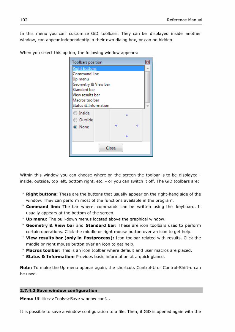
102 Reference Manual
In this menu you can customize GiD toolbars. They can be displayed inside another window, can appear independently in their own dialog box, or can be hidden.
When you select this option, the following window appears:
Within this window you can choose where on the screen the toolbar is to be displayed - inside, outside, top left, bottom right, etc. - or you can switch it off. The GiD toolbars are:
Right buttons: These are the buttons that usually appear on the right-hand side of the window. They can perform most of the functions available in the program.Command line: The bar where commands can be written using the keyboard. It usually appears at the bottom of the screen.Up menu: The pull-down menus located above the graphical window.Geometry & View bar and Standard bar: These are icon toolbars used to perform certain operations. Click the middle or right mouse button over an icon to get help.View results bar (only in Postprocess): Icon toolbar related with results. Click the middle or right mouse button over an icon to get help.Macros toolbar: This is an icon toolbar where default and user macros are placed.Status & Information: Provides basic information at a quick glance.
Note: To make the Up menu appear again, the shortcuts Control-U or Control-Shift-u can be used.
2.7.4.2 Save window configuration
Menu: Utilities->Tools->Save window conf...
It is possible to save a window configuration to a file. Then, if GiD is opened again with the

103Save window configuration
-c option (see Invoking GiD -pag. 5-) and the file in question, the windows are opened in the same place and are the same size as before.
2.7.4.3 Move screen objects
Menu: Utilities->Tools->Move Screen Objects
This option lets you move screen objects (objects that do not belong to the model) such as axes, comments, legends, etc.
2.7.4.4 Coordinates window (only Preprocessing)
Menu: Utilities->Tools->Coordinates window...
Status toolbar:
This option opens a window used to enter points (see Point definition -pag. 21-). It can be used in any place where it is possible to enter a point.
Coordiante window
To accept one point in this window, click Apply or press the Return key.
The Coordinate system option lets you select between:
Cartesian: Cartesian coordinate system.Cylindrical: Enter the radius in the XY plane, the anti-clockwise angle in the XY plane

104 Reference Manual
from the x axis (theta), and the z coordinate.Spherical: Enter the radius, the anti-clockwise angle in the XY plane from the x axis (theta), and the angle with the z axis (phi).
The Local axes option lets you choose:
Global: Global axes.Relative center...: Define a center of coordinates. All new points created with this window will be related to this center. In the window where the relative center is entered, you can select a point from the graphical window with the Pick button.Relative last: The last point entered is the relative center of coordinates.Define new...: This lets you define a new local axes. Once defined, you can select it.
Create new point shows the current way of entering points. The Change button opens the preferences window (see Preferences -pag. 77-) where it can be changed.
The Pick button allows you to select a point from the window which is then inserted in the point fields. From here it can be edited and used.
2.7.4.5 Read batch window
Menu: Utilities->Tools->Read batch window...
A batch file can be read to execute some functions (see Batch file -pag. 45-) or to create an animated view of these operations. This latter case can be performed with the Read batch window.
Read batch window
Once a file is selected, it is possible execute it interactively, and make it stop at interesting points.

105Read batch window
To allow all the movements (rotations and so on) be executed in the same way as originally, the Write rotations in batch option must be flagged in the preferences window (see Preferences -pag. 77- ) when creating the batch.
There are several ways to halt the batch while it is running. One of them is to include stops in the show file section with the Mark break button, and selecting Internal stop. These marks can be saved in the batch file by clicking the Write... button.
The Show info option lets the program write all the usual messages in the GiD messages window.
2.7.4.6 Comments
Menu: Utilities->Tools->Comments...
Comments can be added to images created with GiD by using this command. Click Apply to display the text on the screen as it will appear when printed - either to a file (see Print to file -pag. 56-) or otherwise; comments can be changed at any time by clicking the Comments button in the Utilities menu (either pull-down or Right buttons menus).
2.7.4.6.1 Postprocessing
While displaying results, comments can be automatically generated by switching On the Automatic checkbox of the window, or by menu acces, see Legends -pag. 227- for more information.

106 Reference Manual
Comments customization window
If this option is selected and the comment lines are empty, the program will create its own automatic comments, like these ones:
Load Analysis , step 3
Display Vectors of Displacements , |Displacements| factor 68095.4
Deformation ( x127.348 ): Displacements of Load Analysis 2 , step 8
where the fields which will change when the visualization changes are marked in bold.
You can also create your own automatic comments, just by filling in the comment lines. To tell the program where the result name, analysis name, etc. should be placed, the following fields can be used:
%an: for the analysis name of the current visualized result%sv: for the step value of the current visualized result%vt: for the result visualization type of the current visualized result%vf: for the vectors factor used in the current visualized result (if any)%rn: for the result name of the current visualized result%cn: for the component name of the current visualized result%da: for the analysis name of the current deformation (if any)%ds: for the step value of the current deformation (if any)%dr: for the result name of the current deformation (if any)%df: for the factor of the current deformation (if any)%tcl(): to evaluate a tcl command and display it's result as comment, for instance: "Step id = %sv, correct step value = %tcl(expr $sv * 2.5 + 3.4)" --> will translate to "Step id = 1, correct step value = 5.9".
GiD will substitute the fields for the values of the current visualization. Fields which cannot be filled will be empty.

107Animation controls
2.7.4.7 Animation controls
Menu: Utilities->Tools->Animation controls...
Post toolbar:
Animation controls
This windows lets you create animations while using GiD. Any of these formats can be selected: MPEG, AVI True Color, AVI 15bpp (reduced number of colors: 32768), GIF and FLV (Macromedia Flash Video). AVI with MJPEG compression is also supported. After giving a name and a delay time between frames (for 20 frames per second, a delay of 1/20 = 50 ms. should be entered) the process can be started by clicking on the start button (film roll and arrow icon); the green LED will change to red.
Simply click on the film roll and arrow button to add frame by frame the pictures you want to include in the animation. The Save redraws option tells GiD to save every redraw automatically to the animation file, so no user intervention is needed to store frames.
The animation can be finished at any time by clicking the end button (closed film roll icon); the red LED will change to green.
Note: To avoid problems when trying to view an MPEG format animation in Microsoft Windows, it is strongly recommended that you use the Default menu to select a 'standard' size and click the Resize button. The graphical window will change to this 'standard' size. When you have finished the animation, simply select Default on the menu and click the Resize button and the previous size will be restored.
Note: AVI files with MJPEG compression can be viewed with xanim on Linux and Unix

108 Reference Manual
machines, and with DirectX 8.x installed on Microsoft Windows machines.
2.7.4.8 Animation script
Menu: Utilities->Tools->Animation script...
This window lets you manage and define the movements of the animation. You can chose one of the following movements:
zoom/pan: Define a linear movement from Start view to End view in a specify Duration time.rotation: Define a rotation of the Object or of the Screen by entering Center point, the three axes angles and Duration time.render: Command to change the render state to Normal, Flat or Smooth
The animation of results can also been performed while the movement script is executed. Just check the Do result animation too and set the preferences clicking on Animate results... button.
2.7.4.9 Macros
Menu: Utilities->Tools->Macros...
Toolbar:

109Macros
'Macros' window allows you to create sequences of commands and give them a name. This group of commands can also be recorded from one execution set inside the program.
It is possible to assign a keyboard shortcut to a given macro.
Note: Macros are considered as a user preference and not related to the active model. So, to transfer a set of macros from one user to another it is necessary to copy the appropiated 'Macros.tcl' file (its location is platform dependent)
2.7.4.10 Selection window (only Preprocessing)
Menu: Utilities->Tools->Selection window...
Mouse menu: Contextual->Selection window
For those functions where some entities are to be selected (creation of a surface or a volume, copying entities, etc.), it is possible to use the Selection window. The selection window lets you take control of the selection process.

110 Reference Manual
Selection window
Note: The selection window option is only available in the mouse menu during the selection process.
The selection window has the following options:
Select all: If this option is chosen all entities are selected. If a filter is selected, it is applied to all entities.From, To: This option lets you select a range of entities. If a filter is selected, it is only applied to that range of entities. To see the ID numbers of entities, use the Label command (see Label -pag. 70- ). Mode: There are three selection modes:
Swap : If you select an entity that is already selected, the entity is deselected, and vice versa. Add : In this mode it is impossible to deselect an entity. Only new entities are added to the current selection. Remove : In this mode it is impossible to add entities to the selection. This mode is used to remove entities from the current selection.
Filter: If a filter is selected, only the entities that satisfy the filter criteria will be selected. This menu changes depending on what type of entity is being selected:
PointsHigher entities: You are asked for a value, and all points with this Higher Entity number are selected (Higher Entity number is the number of lines that a point belongs to).Label: Selects all points where a Label is shown or not (On or Off).Material: All points with a chosen material assigned are selected.Condition: All points with a chosen condition assigned are selected.
LinesHigher entities: You are asked for a value, and all lines with this Higher Entity number are selected (Higher Entity number is the number of surfaces that a line belongs to).Label: Selects all lines where a Label is shown or not (On or Off).

111Selection window (only Preprocessing)
Material: All lines with a chosen material assigned are selected.Condition: All lines with a chosen condition assigned are selected.Min. length: Selects only the lines whose length is greater than the given length.Max. length: Selects only the lines whose length is smaller than the given length.Entity type: Selects only the lines which fit the specified type: StLine (Straight Line), ArcLine, PolyLine or NurbLine.
SurfacesHigher entities: You are asked for a value, and all surfaces with this Higher Entity number are selected (Higher Entity number is the number of volumes that a surface belongs to).Label: Selects all surfaces where a Label is shown or not (On or Off).Material: All surfaces with a chosen material assigned are selected.Condition: All surfaces with a chosen condition assigned are selected.Num. sides: All surfaces with a chosen number of sides are selected.Entity type: Type of surface.
VolumesLabel: Selects all volumes where a Label is shown or not (On or Off).Material: All volumes with a chosen material assigned are selected.Condition: All volumes with a chosen condition assigned are selected.Num. sides: All volumes with a chosen number of sides are selected.Entity type: Type of volume.
NodesLabel: Selects all nodes where a Label is shown or not (On or Off).Condition: All nodes with a chosen condition assigned are selected.
ElementsLabel: Selects all elements where a Label is shown or not (On or Off).Material: All elements with a chosen material assigned are selected.Condition: All elements with a chosen condition assigned are selected.Min Angle: Selects only the elements with an angle greater than the figure specified in degrees (see Mesh quality -pag. 194- ). Max Angle: Selects only the elements with an angle smaller than the figure specified in degrees (see Mesh quality -pag. 194- ). Min Edge: Sets the minimum edge length accepted (see Mesh quality -pag. 194- ). Max Edge: Sets the maximum edge length accepted (see Mesh quality -pag. 194- ). Shape quality: Sets the minimum shape quality accepted (see Mesh quality -pag. 194- ). Minimum Jacobian: Sets the minimum jacobian accepted (see Mesh quality -pag. 194- ). Entity type: Type of element (see Element type -pag. 181- ).
Clear: Clears the current selection.
2.7.4.11 Calculator

112 Reference Manual
Menu: Utilities->Tools->Calculator...
vector calculator
This option opens a scalar and vector calculator. Clicking the help button open a dedicated help section.
It is possible to transfer scalar and vector points and distances between the calculator and the main graphical display.
2.7.4.12 Report
Menu: Utilities->Tools->Report...

113Report
report window
This option creates a report in html format to which figures, comments, titles, etc. can be added. This report can be saved to a file and then reloaded in another GiD session where it can be edited or have more information added to it.
2.7.4.13 Notes
Menu: Utilities->Tools->Notes...
This is a simple text editor for writing small notes regarding the model. The content is saved in a file named ModelName.txt, with utf-8 encoding.

114 Reference Manual
2.7.5 Copy
Menu: Utilities->Copy...
Toolbar:
2.7.5.1 Preprocessing
Copy window
Copy is a general function that allows you to select a group of entities and copy them with a movement operation performed, either translation, rotation, mirror, scale or offset.
Select the type of entities to copy. In geometry mode choose between point, line, surface and volume; in mesh mode choose between nodes and elements. All the lower entities belonging to the selected one will automatically be computed. Next, the type of movement needs to be chosen and its parameters defined. The options are:
Rotation: It is necessary to enter two points in 3D, or one point in 2D. These two points define the axis of rotation and its orientation. In 2D, the axis goes from the defined point towards z positive. Enter the angle of rotation in degrees; it can be positive or negative. The direction is defined by the right hand rule. In 2D, the direction is counter-clockwise.Translation: Two points are defined. Relative movements can be obtained by defining the first point as 0,0,0 and considering the second point as the translation vector (see Point definition -pag. 21-).Mirror: Three points are defined (they cannot be in a line). These points form the mirror plane. In 2D, the mirror line is defined by two points.Scale: This is defined by a center and a point. Every coordinate of the point is the scale

115Preprocessing
factor for every x,y,z axis. A scale factor greater than one increases the size, while a scale factor less than one decreases the size. It may also be negative, changing the sign of the corresponding coordinates.Offset: This is defined by one positive or negative scalar magnitude. Each entity will be moved in the direction of its normal, by the magnitude given. In 2D, the normal is considered to lie in the plane z=0. This option works either for lines, surfaces or mesh elements.Sweep: This is an option for copying figures along a line (path line). You can simply copy the figures (and then specify a number of copies) or extrude them. Both methods have basically the same options.
The 'end scale' factor determines how the figure is scaled along the path curve (the scale value starts at 1.0 and varies in a linear way until the 'end scale' value). This scale value must be greater than zero.The extrusion (and the copy) always starts on the start point of the path line. If you select 'twist mode' as on, then the relative position of the figure to copy with respect to the start of the path line is conserved along the line.
Twist mode off and on

116 Reference Manual
In a non-planar curve, there is not only curvature, but also torsion. This may cause some unexpected behaviour, because the figure also has a rotation along the tangent direction of the path:
Natural twist option
Next the 'XY plane' option is used, which makes certain that the initial vector will remain in this plane during extrusion. (In this example, the axis is Z).
The option 'ByDer2' uses the second derivate of the path line as a normal to the plane in which that initial vector has to remain. A rotation along the path line can be forced using the 'Angle' parameter (degrees):

117Preprocessing
Finally, if the path line is a polyline, then the extrusion will be divided into several parts:
Align: This is an option to move figures from a generic position to the desired one. Set the new location specifying three source points and three destination points: the first point defines the exact destination of the source point; the second point is not necessarily the exact destination, but a point over the destination straight line; the third point is not necessarily the exact destination, but a point over the destination plane
Tool to align parts
Other available options are:
Collapse: If this option is set and after the copy operation an entity occupies the same position as an existing one that does not belong to a frozen layer, both entities are converted into one.Do Extrude: This option can be set to either lines, surfaces or volumes. When a movement is selected, the copy is made and lines connecting the old and new points are created. These lines will either be straight lines or arcs depending on the movement

118 Reference Manual
type. If extrude surface is chosen, NURBS surfaces connecting old and new lines will also be created. If Volumes is chosen, the volume contained between old and new surfaces is also created. This option is not allowed when copying volumes.Create contacts: Creates separated contact volumes (see Contact -pag. 143-) for every copied surface. This option is only available when copying surfaces.Maintain layers: If this option is not set the new entities created will be placed in the layer to use; otherwise, the new entities are copied to the same layers as their originals.Multiple copies: By selecting this option and giving the number of repetitions, the selected operation is performed this number of times. This option is not available for mirror.
Note: Entities belonging to a frozen layer (see Layers and groups (only Preprocessing) -pag. 98-), are not checked when sharing old entities.
2.7.5.2 Postprocessing
When you select the Copy tool, the Transformations window appears. This window allows you to repeat the visualization using translation, rotation and mirror transformations, so that GiD can draw a whole model when only a part of it was analyzed.
Transformation: view option

119Postprocessing
Transformation: create option
The types of transformation are:
Translation: This is defined by two points. Relative movements can be obtained by defining the first point as 0,0,0 and considering the second point as the translation vector (see Point definition -pag. 21-).Rotation: It is necessary to enter two points in 3D or one point in 2D. In 3D, these two points define the rotation axis and its orientation. In 2D, the axis goes from the defined point towards z positive. Enter the angle of rotation in degrees. It can be positive or negative. In 3D, the direction is defined by the right hand rule. In 2D, it is counter-clockwise.Mirror: This is defined by three points that cannot be in a line. These points form a plane that is the mirror plane. In 2D, the mirror line is defined by two points.Scale: This is defined by a center and a point. Every coordinate of the point is the scale factor for every x,y,z axis. A scale factor greater than one increases the size, while a scale factor less than one decreases the size. It may also be negative, changing the sign of the corresponding coordinates.
The other available options are:
Copies: By entering the number of repetitions, the operation selected is performed this number of times.
View: The transformation is only for viewing purposes. Show/Hide, Undo and Clear options are enabled.
Show transformation: Allows you to see or hide the model with the transformations active.Show original: allows the user to see or hide the original model over the transformed.Undo: Deletes the last transformation performed. It can be used repeadly to clear

120 Reference Manual
all transformations.Clear: Clears all the transformations in one go.
Create: All the Post information (meshes & results) will be duplicated when performing the transformation.
Crete volume/surfce: creates N-copies of the current meshes.Extrude surface: creates a volume using the selected transformation by extruding the surfaces.
The Apply button tells the program to perform the transformation that has been selected.
2.7.6 Move (only Preprocessing)
Menu: Utilities->Move...
This command works like Copy but moves the entities instead of copying them. The program automatically checks to see if any of the entities must be copied instead of being moved (for example, if they also belong to other higher level entities) and performs the appropriate operation.
Options like Extrude, Multiple copy and Create contacts are disabled for movements.
2.7.7 Status
Menu: Utilities->Status...
Status toolbar:

121Status
Preprocessing status window Postprocessing status window
The Status option gives useful information about general project data.
Note that information given on preprocessing and posprocessing its different.
2.7.8 List
Menu: Utilities->List
Toolbar:

122 Reference Manual
The List command gives information about the selected entities. This information is read-only.
Preprocessing:
Geometric entities: Points, lines, surfaces or volumes:Show information: Number, layer, higher entitie, conditions, number and orientation of contour entities.
Nodes:Show information: Number, layer, higher entitie, conditions and coordinates.
Elements:Show information: Number, layer, higher entitie, conditions, element type (Linear, Triangle, Quadrilateral, Tetrahedra, Hexahedra, Prism, Pyramid, Point, Sphere or Circle) volume of the element and nodes that define the element.
Posprocessing:
Nodes: Show information: coordinates, which elements uses this node, the current visualized result, and all other nodal results defined over the selected nodes.
Elements: Show information: connectivity, the gauss points defined on the selected elements, the current visualized result, and all other results defined over the gauss points of the selected elements. For spheres, their raius are also shown, and for circles, their radius and nomral.
All this information can be sent to the active report (see Report -pag. 112-) by using the button.
2.7.9 Mass (only Preprocessing)
Menu: Utilities->Mass
Information about physical properties is given: lengths of lines, center of mass, areas of surfaces, volumes of solids. It works for both the geometry and the mesh.
2.7.10 Renumber (only Preprocessing)
Menu: Utilities->Renumber
When creating new entities, the label of the new entity will be the lowest number greater than 0 that still does not exist for this entity type. If an entity is deleted, a gap is left in the labels list. This gap will be filled with a new entity, but it is also possible to renumber the geometry, changing the previous entity labels. There are no problems with materials and conditions applied to entities.

123Renumber (only Preprocessing)
In geometry mode, the renumbered entities are the geometrical ones.
In mesh mode, the renumbered entities are the mesh ones. In this case, renumbering not only fills the gaps in the labels list but also changes the node numbers so as to minimize the difference in node numbers within each element. This can be useful when the calculating module uses band or skyline storage methods.
The nodes renumeration algorithm can be set with the variable 'RenumberMethod' (see Preferences -pag. 77-)
Accepted values are:
-2 : Avoid nodes and elements renumeration, entities numbers are set increasingly when they are generated.
-1 : Avoid nodes renumeration, nodes numbers are set increasingly when they are generated
0 : Geometrical algorimth, ordered by the distance to some coordinate. It is the default value
1 : Reverse Cuthill-McKee algorimth, similar to the previous one, but following element's connectivities
2 : ordered following the XYZ axes, interesting for special cases with geometry aligned to the axes
Note: When generating a mesh using GiD it is not necessary to use this command because it is automatically applied when generating the mesh.
Note: Negative numbers in this variable are understood as internal checks and tests, so they are not loaded from the model if it's meshing preferences are set.
2.7.11 Id
Menu: Utilities->Id
This command gives the label and coordinates of an existing or new point. Different options for getting information about an existing point are available in the Contextual menu.
2.7.12 Signal
Menu: Utilities->Signal
With this option you can select one entity (a point, line, surface or volume), and a pair of crossed red lines will signal the center of the entity in the graphical window.
They must be existing entities, except the special case of points or nodes, where they can be existing or defined with any of the usual methods.

124 Reference Manual
The Superpose Lines option (in the Contextual menu) is useful when in render mode. Depending whether it is set or not, the crossed red lines will either be in front of the object or partially hidden by the model.
2.7.13 Swap normals (only Preprocessing)
Menu: Utilities->Swap normals
This command can be applied to lines or surfaces (in geometry mode) or to elements (in mesh mode). A selection is made (see Entity selection -pag. 26-) and the orientation of the selected entities is inverted.
Viewing commands (zoom, rotation, etc.) can be applied and the normals will remain on the screen.
When this command is applied to surfaces or mesh elements, you can choose one of the following options:
Select: Inverts the direction of the normals of the selected surfaces.Make coherent: Inverts the normals of all selected surfaces or elements so that all of them have their normal in the same direction as adjacent entities. This direction is arbitrary, but is common to all adjacent entities.Select by normal: You are prompted to enter a vector and all selected entities' normals are swapped so as to have their normal in the same direction (dot product positive) as the given vector.Pointing inside volumes: the normal of skin surfaces of selected volumes are swapped to point inside its volume. Surfaces shared by more than one volume are not swapped.
Note: With the Color option set (available in the Contextual mouse menu), all surfaces or elements are drawn in filled color. Their front side will be drawn in their regular color, and their back face in yellow.
Note: Volumes are correctly oriented by GiD, regardless of their surface orientation.
2.7.14 Distance
Menu: Utilities->Distance
The Distance command gives the distance between two existing or new points.
2.7.15 Dimension
Menu: Utilities->Dimension

125Dimension
With the dimensions option it is possible to add textual information to your model. This information can be moved to a different layer or deleted.
The following options are available:
Menu: Utilities->Dimension->Create
Vertex: Shows the coordinates of a vertex. Click over an existing point and then click where you want the dimension to be written.Distance: Shows the distance between two points. You have to select two points and then click where you want the dimension to be written.Angle: Shows the size of an angle in degrees. You have to select three points and then click where you want the dimension to be written.Radius: Shows the center and radius of an arc. You have to select an existing arc and then click where you want the dimension to be written.Text: Shows a text string defined by the user. Enter the text and click where you want the text to be written.
Menu: Utilities->Dimension->Delete
Deletes a "dimension". Select the dimension you want to delete and press ESC.
Menu: Utilities->Dimension->Edit
Select the dimension you want to edit, change the text, and click OK.
Menu: Utilities->Dimension->ShowBox
This option lets you change the appearance of a "dimension"; a "dimension" can be drawn

126 Reference Manual
with or without a box. Choose ShowBox on or off, select a "dimension", and press ESC.
2.7.16 Repair model (only Preprocessing)
Menu: Utilities->Repair model
This option checks the coherence of the database information. Only use it if there are problems. When used, a window notifies you of any repaired items and may give some warnings about incorrect entities.
2.7.17 Collapse nodes (only Postprocessing)
Menu: Utilities->Collapse nodes
Collapses nodes that are together in a set.
2.7.18 Join (only Postprocessing)
Menu: Utilities->Join
Joins several sets into one.
2.7.19 Delete (only Postprocessing)
Menu: Utilities->Delete
Deletes meshes, sets and cuts.
2.7.20 Texture (only Postprocessing)
Menu: Utilities->Texture
In GiD it is also possible to assign a texture to a Set. Inside the Utilities -> Texture menu there are several options:
View No / Fast / Nice: switches between viewing the textures over the sets or not. When the texture is small and a pixel of the textures must be drawn over several pixels on the screen, the Fast mode just draws the pixels using the 'nearest neighbor' policy, while the Nice mode tries to interpolate the colours of the pixels from the original.
Add Screen Map / To 4 sided set / BoundImg to BoundSet: maps a texture to a set. ScreenMap: by picking four points over the screen, GiD projects the texture parallel to the screen, over the underlying sets. 4 sided set: GiD tries to match the 4 sides of the texture to the 4 sides of the set. The best results are achieved using quadrilateral sets which are more or less flat, at least in one direction.

127Texture (only Postprocessing)
BoundImg to BoundSet: GiD looks for the border of the texture inside the image file and tries to glue it to the border of the set, for instance a texture circle to a circle set.
Change Flip Horiz. / Vert.: changes the orientation of the texture once it is applied to the Set.
Note: When the display style of the visualization is changed, for instance from Body to Body Boundaries, the visualization of the texture is switched off. To view the texture, just select Utilities -> Texture -> View -> Fast/Nice.
Once the texture is applied to a Set, any deformed of the Set leads to a corresponding deformation of the texture. In this way the deformed texture can be visualized.
2.8 Help Menu
GiD provides a help system. You can access the following sections: Reference Help, Customization, Tutorials, What is new and FAQs (Frequently Asked Questions)
The help window provides two ways of accessing a given topic:
a) through a table of contents shown as a tree
b) through a search engine.
GiD help window
From the Help menu you can also register GiD (see Register GiD -pag. 128-) and Problem Types (see Register Problem type -pag. 129-).
2.8.1 Help
Menu: Help->Help
Toolbar:

128 Reference Manual
This option gives access to the GiD reference manual help (this manual), that shows information about the commands classified by menus.
Beginners must start following the tutorials of the user manual. The reference manual must be consulted to know more about specific GiD features, but it is not a learning manual.
2.8.2 Customization help
Menu: Help->Customization help
This option gives access to the Customization part of GiD Help.
Beginners could ignore this manual and follow the tutorials of the user manual. The information is important for advanced users that want to adapt GiD for their own simulation program.
2.8.3 Tutorials
Menu: Help->Tutorials
This option gives access to some tutorials which help the user to start learning GiD from a practical point of view.
It cover topics to progressive learn how to create and modify a geometry, to generate a calculation mesh, to visualize the results, and an introduction about the possibilities to adapt GiD for your own simulation code.
2.8.4 What is new
Menu: Help->What is new
This option gives access to a list of the new developments present between versions of GiD.
2.8.5 FAQ
Menu: Help->FAQ
This option gives access to a list of the Frequently Asked Questions (FAQ) related with GiD.
2.8.6 Register GiD
Menu: Help->Register...
In order to take advantage on the full capabilities of GiD, you need to register a password that can be obtained from www.gidhome.com. From this site you can obtain a permanent or temporary password.

129Register GiD
If there is some USB memory stick plugged then GiD will show a window with a list to allow the selection of this device (portable licence) or the local machine (local licence). Highlight the one you want and press Select.
USB or Local machine selection
The password must be typed in the window shown below.
GiD register window
If you have previously registered your current copy of GiD, the password can be reloaded by clicking the icon and selecting the folder where the old password is.
In case of floating licences the 'machine and password' are replaced by the 'IP' of the 'passerver' password server.
After registering either a permanent or temporary password you will be able to generate and postprocess an unlimited number of nodes and elements.
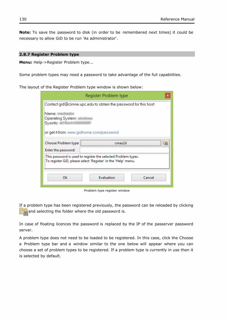
130 Reference Manual
Note: To save the password to disk (in order to be remembered next times) it could be necessary to allow GiD to be run 'As administrator'.
2.8.7 Register Problem type
Menu: Help->Register Problem type...
Some problem types may need a password to take advantage of the full capabilities.
The layout of the Register Problem type window is shown below:
Problem type register window
If a problem type has been registered previously, the password can be reloaded by clicking and selecting the folder where the old password is.
In case of floating licences the password is replaced by the IP of the passerver password server.
A problem type does not need to be loaded to be registered. In this case, click the Choose a Problem type bar and a window similar to the one below will appear where you can choose a set of problem types to be registered. If a problem type is currently in use then it is selected by default.

131Register Problem type
Choose Problem type window
2.8.7.1 Customizing Problem type registration
GiD provides a default validation when registering a module or problem type. This consists of checking that the password is not empty. If the password is valid, GiD appends a line to the file <problem type>/password.txt similar to this:
hostname password # 2008 01 19 Password for Problem type '/pathroot-to-problem-type/problemtype.gid'
This default validation can be overridden, but this involves Tcl programming. For a description of how to provide a custom password validation see ValidatePassword node from Customization Manual.
2.8.8 Register from file
Menu: Help->Register from file
This option is used to register GiD and all problem types stored in a *.pwd file. This option is interesting in order to register several modules and GiD in a single step.
The contents of a .pwd multiple passwords file is simply a text file with a line for each password with this syntax:
machine password # Password for GiDmachine password # Password for module 'problemtype_a.gid'

132 Reference Manual
machine password # Password for module 'problemtype_b.gid' ...
where :
machine is the machine name shown by Help->Register GiD... in this computer.password is the local password for this machine, without - separators. In case of floating licences 'machine and password' are replaced by the 'IP' of the 'passerver' password server.'problemtype_x.gid' is the relative path of the problemtype (relative from the \problemtypes folder).
Note: the sentence "Password for module" must be used for problemtype passwords only, otherwise it will be considered as a password for GiD.
2.8.9 Visit GiD web
Menu: Help->Visit GiD web
This command open an Internet browser that takes you to the GiD homepage (http://www.gidhome.com).
2.8.10 Check for updates
Pops up a window telling if your version is up to date. If there is a newer GiD version available you can download it.
An internet connection is needed .
Note: this ftp connection could be forbidden by some firewall configurations.
2.8.11 About
Menu: Help->About...
This command gives information about the version of the program.
Pressing the 'More' button will show more information about the system, current graphic card configuration and used libraries.

PREPROCESSING
133
3.1 Geometry Menu
All available geometrical operations - generating, manipulating and deleting entities - are included in this chapter.
3.1.1 View geometry
Menu: Geometry->View geometry
Toolbar:
This command changes from mesh visualization to geometry visualization.
3.1.2 Create
This menu is for the generation of all the different possible geometrical entities. Usually, new entities are created inside the current layer (see Layers and groups (only Preprocessing) -pag. 98-).
3.1.2.1 Point
Menu: Geometry->Create->Point
Individual points are created by entering each point in the usual way (see Point definition -pag. 21-). The points can then be joined together to form lines.
Caution: It is impossible to create new points joining old ones.
The Number option lets you choose the label that will be assigned to the next point created. If a point with this number already exists, the old line changes its number. This option is used for example to automatize thinks in macros, knowing the identifier of the entitiy because it is forced.
3.1.2.2 Straight line
Menu: Geometry->Create->Straight line
Toolbar:
134 Reference Manual
To create a straight line, start by entering just two points (see Point definition -pag. 21- ), and then continue entering points in order to create more lines from the first one. Every part of the total line created is an independent line.
It is important to note that when creating lines, new points are also being created (if existing ones are not used).
The Close option joins the first point and the last point created with a straight line and finishes.
The Undo option undoes the creation of the last point (if new) and the last line. It is possible to continue undoing all the way back to the first point.
The Number option lets you choose the label that will be assigned to the next line created. If a line with this number already exists, the old line changes its number.
If Join is chosen, it is maintained for all points until No join is selected.
3.1.2.3 NURBS line
Menu: Geometry->Create->NURBS line
Toolbar:
Interpolation / Fitting
NURBS are non-uniform rational B-splines. They are a type of curve that can interpolate a set of points. NURBS can also be defined by their control polygon, another set of points that the curve approximates smoothly.
There are two ways of creating a NURBS line using this command, either by entering some interpolated points or entering the points that form the control polygon.
The Undo option undoes the creation of the last point; this can be done all the way back to the first point.
By default, a NURBS will be a cubic polynomial passing through all the points. However, this option can be changed by calling ByControlPts, which defines NURBS by their control polygon. This polygon is a set of points where the first and the last points match the first and last points of the curve. The rest of the points do not lie on the curve. It can be assumed that the curve approximates the points of the polygon in a smooth way. In this case, the user chooses the degree of the curve, which will be the degree of the connected polynomials that define the NURBS.
Instead of entering interpolated points, the Fitting option lets you approximate a line using

135NURBS line
a minimum squared criteria. You also have to select the degree of approximation for this curve.
When defining interpolating curves, you can choose to define the tangents to one or both ends (using the Tangents option). These tangents can be customized, in that they can either be defined by picking their direction on the screen or by considering an existing line as a tangent to the NURBS if it follows a previous curve (the option ByLine). The Next option allows only one tangent to be defined.
In this way, it is possible to create a closed NURBS by selecting the initial point as the end one and choosing one of the options 'Tangent', 'Next', or 'ByLine'.
When a NURBS has been created, all the interior points (except the first and last) are not really entity points unless they previously existed.
The Number option lets you choose the label that will be assigned to the next created line. If a line with this number already exists, its number is changed.
To enter rational weights on the curve, the Edit NURBS line/surface command (see Edit NURBS -pag. 151- ) can be used.
Surface constant:
This option allow the creation of a curve on a parametric surface setting the parameter u or v to a constant value specified by the user.
3.1.2.4 Parametric line
Menu: Geometry->Create->Parametric line
Tool to create a parametric approximated curve

136 Reference Manual
Parametric line window
The data that must be input are the mathematical formulae of the coordinates X(t), Y(t) and Z(t), where 't' is the parameter of the curve, and its value belongs to the interval [ t0-t1 ]. The curve is created by approximation and is a NURBS (Non-Uniform Rational B-Spline) which is created with N points. In GiD these kinds of curves are cubic (order 3).
The valid mathematical funcions are all Tcl functions:
+ - * / %abs cosh log sqrt acos double log10 srand asin exp pow tan atan floor rand tanh atan2 fmod round ceil hypot sin cos int sinh
EXAMPLE
We fill the formula bars with the expression of a conic helix.
That helix starts with radius R0=4 and finishes with radius R1=1, performing N=3 turns
from t=0.0 to t=1.0, the height also changes from 0 to H=5.

137Parametric line
Example of a conic helix with a unique curve or with points only
3.1.2.5 Polyline
Menu: Geometry->Create->Polyline
Toolbar:
A polyline is a set of at least two other lines of any type (including polylines themselves). Every line must share one or two of its endpoints with the endpoints of other lines.
There are two possible ways to create a polyline, either by selecting one line and searching the rest until a corner or end is reached, or by selecting several lines (see Entity selection -pag. 26-). In the case of the latter, the order of selection is not important but all of them must join each other by sharing common points.
Polylines are drawn in green to show the difference between the other lines, which are drawn in blue.
Polylines are widely used when creating 4-sided surfaces (see 4-sided surface creation -pag. 145-) and automatic 4-sided surfaces (see Automatic 4-sided surface creation -pag. 146-).
When deleting a polyline, all its lines are deleted. When exploding it (see Polyline -pag. 150-), the polyline will disappear and its individual lines will appear.
It is not possible to create third level polylines: one former polyline can be included inside another, but this is the limit and these two cannot be included within a further polyline.

138 Reference Manual
The Number option lets you choose the label that will be assigned to the next created line. If a line with this number already exists, its number is changed.
3.1.2.6 Arc
Menu: Geometry->Create->Arc
Toolbar:
To create an arc you can either enter three points (By 3 points, see Point definition -pag. 21-) or enter a radius and the two tangent lines at the arc's ends (Fillet curves).
It is important to note that when creating an arc, new points are also being created (if existing ones are not being used).
An arc that begins and ends at the same point (i.e. where the first and third points are the same) will be created as a circle. An arc will always include the second point that is entered, though this one is only used as a reference and, if it is not an existing point, is automatically erased when the arc is created.
The Undo option undoes the creation of the last point (if it is a new one). It is possible to continue undoing all the way back to the first point.
The Fillet curves option lets you input a radius and select two lines that share one common point. An arc will then be created and the two lines will be modified to be tangent and continuous with this new arc.
To convert one arc to another one with the same center and in the same plane but with a complementary angle, the Swap arc command can be used (see Swap arc -pag. 150-).
3.1.2.7 NURBS surface
Menu: Geometry->Create->NURBS surface
Toolbar:
NURBS are non-uniform rational B-splines. They are a type of surface that is defined by its control polygon (one set of points that the surface approximates smoothly), one set of knots for the two directions u and v (a non-decreasing list of real numbers between 0 and 1) and, optionally, one set of rational weights.
To draw the isoparametric lines in u,v=0.5, check the surface drawing type option in the
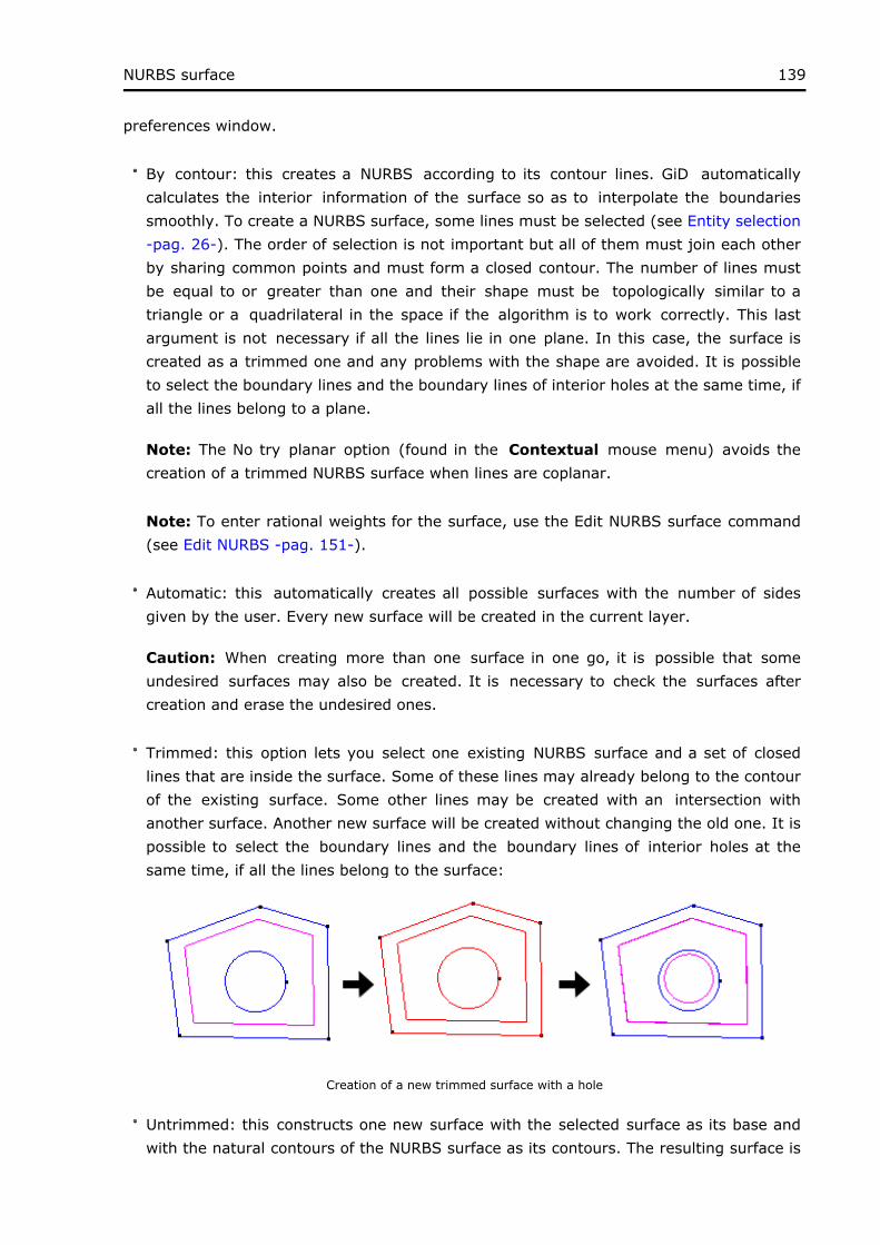
139NURBS surface
preferences window.
By contour: this creates a NURBS according to its contour lines. GiD automatically calculates the interior information of the surface so as to interpolate the boundaries smoothly. To create a NURBS surface, some lines must be selected (see Entity selection -pag. 26-). The order of selection is not important but all of them must join each other by sharing common points and must form a closed contour. The number of lines must be equal to or greater than one and their shape must be topologically similar to a triangle or a quadrilateral in the space if the algorithm is to work correctly. This last argument is not necessary if all the lines lie in one plane. In this case, the surface is created as a trimmed one and any problems with the shape are avoided. It is possible to select the boundary lines and the boundary lines of interior holes at the same time, if all the lines belong to a plane.
Note: The No try planar option (found in the Contextual mouse menu) avoids the creation of a trimmed NURBS surface when lines are coplanar.
Note: To enter rational weights for the surface, use the Edit NURBS surface command (see Edit NURBS -pag. 151-).
Automatic: this automatically creates all possible surfaces with the number of sides given by the user. Every new surface will be created in the current layer.
Caution: When creating more than one surface in one go, it is possible that some undesired surfaces may also be created. It is necessary to check the surfaces after creation and erase the undesired ones.
Trimmed: this option lets you select one existing NURBS surface and a set of closed lines that are inside the surface. Some of these lines may already belong to the contour of the existing surface. Some other lines may be created with an intersection with another surface. Another new surface will be created without changing the old one. It is possible to select the boundary lines and the boundary lines of interior holes at the same time, if all the lines belong to the surface:
Creation of a new trimmed surface with a hole
Untrimmed: this constructs one new surface with the selected surface as its base and with the natural contours of the NURBS surface as its contours. The resulting surface is
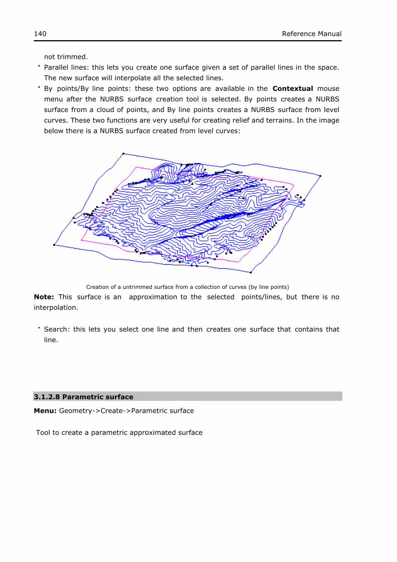
140 Reference Manual
not trimmed.Parallel lines: this lets you create one surface given a set of parallel lines in the space. The new surface will interpolate all the selected lines.By points/By line points: these two options are available in the Contextual mouse menu after the NURBS surface creation tool is selected. By points creates a NURBS surface from a cloud of points, and By line points creates a NURBS surface from level curves. These two functions are very useful for creating relief and terrains. In the image below there is a NURBS surface created from level curves:
Creation of a untrimmed surface from a collection of curves (by line points)
Note: This surface is an approximation to the selected points/lines, but there is no interpolation.
Search: this lets you select one line and then creates one surface that contains that line.
3.1.2.8 Parametric surface
Menu: Geometry->Create->Parametric surface
Tool to create a parametric approximated surface

141Parametric surface
Parametric suface windowExample creating lines U and V of surface
parametrization
The required input data are the mathematical formulae of the coordinates X(u,v), Y(u,v) and Z(u,v), where 'u' and 'v' are the parameters of the surface, and its value belongs to the intervals set in 'u in' and 'v in' respectively. The surface is created by approximation and is a NURBS (Non-Uniform Rational B-Spline), which is created with 'Number of points U' x 'Number of points V' points. In GiD these kinds of surfaces are cubic (order 3).
The valid mathematical funcions are all Tcl functions:
+ - * / %abs cosh log sqrt acos double log10 srand asin exp pow tan atan floor rand tanh atan2 fmod round ceil hypot sin cos int sinh
3.1.2.9 Contact surface
Menu: Geometry->Create->Contact surface
Contact surfaces are defined as being between two lines that are physically in the same place, but which have different line and point entities. From a contact surface, it is possible to generate contact elements, to be used by some calculation algorithms, which define a special contact between these two bodies.
Using contact surface entities is like a meshing specification. In this way, equal meshes will be generated for the two lines, ensuring a one-to-one relationship between nodes.
Choose the Contact surface option from the menu, and then select some lines on both bodies.
Contact elements are, by default, 4-node planar quadrilaterals. However, you can select 2-node lines for all cases (see Element type -pag. 181-).

142 Reference Manual
The 4-node planar quadrilaterals can be converted to the 8-node or 9-node for the quadratic case.
You can also select no mesh for the contact entity. This makes it possible to have exactly the same mesh for both lines but without any additional element between them.
3.1.2.10 Surface mesh
Menu: Geometry->Create->Surface mesh
With this option a Surface mesh can be created by selecting triangular or quadrilateral mesh elements (see Surface mesh -pag. 41-).
3.1.2.11 Geometry from mesh
Menu: Geometry->Create->Geometry from mesh
This option converts all our mesh model (only surface mesh, triangles and quadrilateral) to a geometry model, obtaining a NURBS surfaces based definition. Creates a group of new layers called "Reconstruction", inside you will see two new layers: the first "All Lines And Points" contains lines and point and the second "Reconstructed Nurbs" the surfaces. If some surface couldn't be reconstructed it will appear a third layer called "SurfMeshes Not Reconstructed" containing the remaining parts converted in Surfmeshes, see more infomation about Surf Mesh -pag. 41-.
3.1.2.12 Volume
Menu: Geometry->Create->Volume
Toolbar:
A volume is an entity formed by a closed set of surfaces that share the lines between them.
To create a volume, some surfaces must be selected (see Entity selection -pag. 26- ) using the By contour option. The order of selection is not important but all of them must join each other by sharing common lines and they must form a closed contour.
If there is an error and the volume is not created, a window appears with some useful information.
The Search option lets you select one surface and create one of the volumes that contains this surface.

143Volume
Volumes and their surfaces are automatically orientated so that they are meshed correctly.
An additional feature allows the selection of surfaces that form the outer part of the volume as well as the ones that form the holes at the same time. In this case, GiD automatically recognizes the holes.
The Automatic 6-sided volumes option creates all possible volumes that have 6 sides (contour surfaces). It can be applied several times over the geometry and volumes are not repeated. Every new volume will be created in the current layer.
This can be useful for structured meshing (see Structured -pag. 171- ).
3.1.2.13 Contact
Menu: Geometry->Create->Contact volume
Contact volumes are defined between two surfaces that are physically in the same place but with different surfaces, lines and points. From a contact volume, it is possible to generate contact elements, to be used by some calculation algorithms, which define special contact between two bodies.
Those equivalent surfaces can be in the same location or can be separated by a movement (separated contact volume). The result will be equal meshes, ensuring a one-to-one relationship between nodes.
Choose 'contact volume' from the menu, and then select the surfaces. GiD automatically searches for possible contacts, combining the selected surfaces in pairs.
Contact elements are, by default, 8-node hexahedra or 6-node prisms (depending on the surface mesh). However, you can select 2-node lines for all cases (see Element type -pag. 181-).
The result elements can be also quadratic.
You can also select no mesh for the contact entity. This makes it possible to have exactly the same mesh for both surfaces but without any additional element between them.
When creating contact volumes, GiD internally checks what surfaces occupy the same location in the space and creates the contact, therefore there is no need to specify what surfaces have to be in contact. For this reason, several surfaces can be selected at once and GiD performs the contact automatically, indicating the number of contact volumes that have been generated.
One feature of GiD is the option to create 'contact separated volumes' for surfaces that are not physically in contact.

144 Reference Manual
For these separated volumes, GiD internally checks whether a unique solid-rigid movement exists between two surfaces and creates the contact. There is the possibility that multiple solid-rigid movements may exist. In this situation, GiD asks for the point image of a source point to define the movement and, consequently, applies the right contact.
3.1.2.14 Object
Menu: Geometry->Create->Object
Toolbar:
With this command it is possible to create the following kinds of objects:
RectanglePolygonCircleSphereCylinderConePrismTorus
When creating an object, GiD asks for a center and a normal. To enter the coordinates of the center you can click on the screen or select an existing point (see Point definition -pag. 21- ). To enter the normal, GiD displays a window where you can choose one of the three axes or enter the coordinates of a point.
Window to define the direction of the normal to the plane
The In screen button in the Enter normal window lets you manually enter the coordinates of the point which defines the normal: you can directly click on the screen or pick an existing point using the Join option in the Contextual mouse menu.

145Object
When using the commands sphere, cylinder, cone, prism or torus, the volume of the object is also created.
3.1.2.15 Old types
3.1.2.15.1 4-sided surface creation
The 4-sided surface has been substituted by the NURBS surface (see NURBS surface -pag. 138- ). This new entity has all the functionality of the old one.
Note: It is still possible, however, to access to this function with the Right buttons menu (see Tools -pag. 101- ).
A 4-sided surface is an entity formed by a closed set of four lines in the space. Its mathematical definition is a bilinear Coon's surface. The surface is totally defined by the shape of the lines, with no information about the interior. This means that it will sometimes be necessary to use more surfaces to obtain a good shape definition.
To create a 4-sided surface, several lines must be selected (see Entity selection -pag. 26- ). For the creation of a 4-sided surface defined by three lines, it is necessary to divide one of the lines into two pieces (see Divide -pag. 147- ). The order of selection is not important, but all of them must join each other by sharing common points and they must form a closed contour. If it cannot be created, information about the endpoints is displayed in a window.
In order to make one or more lines form parts of a polyline (see Polyline -pag. 137- ), select the entire polyline as one of the lines and GiD will automatically select the piece or pieces of the polyline that are required. Using this facility, non-conforming surfaces can be created. This means creating a surface by using the entire line on one side of the polyline, and creating more than one 4-sided surface by using parts of it on the other side.
When selecting more than four lines, GiD will automatically search for all the possible 4-sided surfaces that can be created with these lines. This allows the creation of many surfaces at the same time.
The Automatic button is equivalent to automatic 4-sided surface creation (see Automatic 4-sided surface creation -pag. 146- ).
If the surfaces lie on the z=0 plane, the orientation of the surfaces will be anti-clockwise in this plane (normal vector points towards z positive). Otherwise, the orientation will be arbitrary. This can be checked with the DrawNormals command (see Normals (only Preprocessing) -pag. 71- ).
The Number option lets you choose the label that will be assigned to the next created surface. If a surface with this number already exists, the old line changes its number.

146 Reference Manual
Caution: When creating more than one surface at a time, some undesired surfaces may also be created. It is necessary to check the surfaces after creation and erase the undesired ones.
3.1.2.15.2 Automatic 4-sided surface creation
The 4-sided surface has been substituted by the NURBS surface (see NURBS surface -pag. 138-). This new entity has all the functionality of the old one.
Note: It is still possible, however, to access to this function with the Right buttons menu (see Tools -pag. 101-).
Inside this option, GiD creates as many 4-sided surfaces as it can find. Every new surface will be created in the current layer.
Caution: When creating more than one surface at a time, some undesired surfaces may also be created. It is necessary to check the surfaces after creation and erase the undesired ones.
3.1.2.15.3 Planar surface creation
The planar surface has been substituted by the NURBS surface (see NURBS surface -pag. 138- ). The latter automatically detects if boundary lines lie in a plane and creates a planar NURBS.
Note: It is still possible, however, to access this function with the Right buttons menu (see Tools -pag. 101- ).
A planar surface is an entity formed by a closed set of lines, all of them lying on the same plane. These lines must share some common endpoints.
To create a planar surface, some lines must be selected (see Entity selection -pag. 26- ). The order of selection is not important but all of them must join each other by sharing common points and must form a closed contour. If all lines are not in the same plane the surface is not created.
It is possible to add holes to a planar surface. To do so, it is first necessary to create the outside planar surface. After this, press the Hole button and select the created surface. Then select lines that form every hole, one by one. Finish with escape (see Escape -pag. 29- ). It is also possible to define the surface and holes at the same time, by selecting all the curves.
If the surfaces lie on the plane z=0, the orientation of the surfaces will be anti-clockwise in
147Planar surface creation
this plane (the normal vector points towards z positive). Otherwise, orientation will be arbitrary. This can be checked with the DrawNormals command (see Normals (only Preprocessing) -pag. 71- ).
3.1.3 Delete
Menu: Geometry->Delete
Toolbar:
The deletion of entities can be done in two ways: at one level (point, line, surface or volume) or erasing all entities at once. A selection is made (see Entity selection -pag. 26-) in both cases. After pressing escape (see Escape -pag. 29-), the entities are erased.
To undo the selection of entities, press Clear selection in the Contextual menu.
Entities that form the basis of higher entities cannot be erased. For example, if a surface is created over some lines, it is necessary to erase the surface before erasing the lines.
3.1.4 Edit
These are the GiD editing options for geometrical entities:
3.1.4.1 Move point
Menu: Geometry->Edit->Move point
By using this command, an existing point is selected and moved. The new position is entered in the usual way (see Point definition -pag. 21-). If the new position is an existing point (when using join), GiD will determine the distance between the points and ask if they should be joined. If the answer is yes, both points are converted into one. Any lines of surfaces that include the point in question will be moved accordingly in order that any links are maintained; this may lead to these lines or surfaces being distorted.
3.1.4.2 Divide
Menu: Geometry->Edit->Divide
The Divide command can be applied either to lines, polylines , surfaces (including trimmed surfaces), and volumes.
Polylines: In the case of polylines, an existing interior point must be chosen. The

148 Reference Manual
polyline will be converted into two lines that may or may not be polylines.
Polyline division has the option Angle which allows you to divide the polyline at all the points where the angle between the sub-lines is greater than a given value.
Caution: An interior point must belong to the first level of a polyline (see Polyline -pag. 137-).
In the case of lines and surfaces, once the entity has been selected the division can be done in several ways:
Number of divisions: The line or surface will be converted into equally spaced pieces. In the case of surfaces it is necessary to give the division direction as u or v. Near point: With this option one point must be selected near the line or the surface. Points inside the entities can be selected (see Point in line -pag. 25-, or Point in surface -pag. 25-). The line or the surface will be divided into two entities near that point. In the case of surfaces it is necessary to give the division direction as u or v.Parameter: One factor is given between 0.0 and 1.0 and the entity will be divided where the parametric variable takes that value. In the case of surfaces it is necessary to give the division direction as u or v.Relative length: (lines only) One factor is given between 0.0 and 1.0 to divide the line with relative arc length ratio equal to the selected factor. (Same concept as Parameter if the curve was arc length parameterized).Length: (lines only) The length of the resulting divided lines is given, and GiD divides the line into as many lines as it can. If the length given is bigger than the length of the selected line, no division is made.
Split: (surfaces or volumes) The surface/volume will be divided following the divide lines/surfaces. These lines/surfaces must share points/lines with the to be splitted (Command: Geometry Edit SplitSurf/SplitVolume ).
Note: After the division, the old entity disappears and the new entities are created.
3.1.4.3 Join
Menu: Geometry->Edit->Join
With this option you try to join connected entities.

149Join
Join surfaces:
Rebuilt by boundary:A group or connected surfaces must be selected in order to try to create a single approximated surface.
QuickJoin (default option)NoQuickJoin. More parameters are available.
IsProjectable : Yes or NotWeightBoundary: Yes or NotNumApproxPointsTolerance
Join only coplanars:A group of surfaces must be selected, and automatically are detected subgroups of planar parts that are joined in single planar surfaces.
TolAngle could be set to determine when two surfaces are coplanar
Join volumes:
Two or more volumes connected by shared surfaces are joined in a single one.
By default, if 'NoDeleteOriginalVolumes' was set, the source volumes and its dependent entities will be deleted.
3.1.4.4 Line operations
Menu: Geometry->Edit->Line operations
With this option you can edit groups of lines with respect to their topology and shape.
Join lines end points:
With the command Join lines end points, two lines must be selected. GiD determines the distance between the two closest endpoints, draws both points, and asks for confirmation. If one of the lines is a polyline, interior points are also considered. If accepted, the points are converted into one and the lines are distorted. The new point will then take the place of the first line's point.
(See Move point -pag. 147- for another method of converting two points to one.)
Caution: The second selected line cannot have higher entities (the second point is moved to the first).
Force to be tangent:
With the command Force to be tangent, two lines (which share at least one point) must be selected. They must be NURBS lines, otherwise they will be rejected. You are asked to

150 Reference Manual
enter the maximum angle between lines to accept the operation, and GiD will modify the selected NURBS lines and force them to be tangents at their common point.
3.1.4.5 Swap arc
Menu: Geometry->Edit->Swap arc
This command lets you select and alter arcs. Lines that are not arcs are rejected. When you confirm the operation, the arc is converted to a new arc with the same center and in the same plane but opposite the old one. The old arc disappears and the angle of the new arc will be complementary to the angle of the old arc.
Caution: Arcs belonging to higher entities cannot be swapped.
3.1.4.6 Polyline
Menu: Geometry->Edit->Polylines
Explode polyline:
This command lets you select which polylines you wish to explode; lines that are not polylines or have higher entities or conditions are rejected. After confirmation, the polylines are exploded and converted back to their original lines. Polylines then disappear (see Polyline -pag. 137-).
Edit polyline:
The command Edit Polyline allows you to select which polylines you wish to edit; lines that are not polylines are rejected. It is possible to choose several options for the polylines:
Use points: When meshing this polyline, there will be at least one node at every point location that defines the polyline. These will be the endpoints of interior lines.Not use points: When meshing this polyline, the mesh generator ignores the points and therefore the nodes will be placed anywhere. This is the default option. Nodes will only be put in the position of a point if there is a 4-sided surface over a part of a polyline (see Automatic 4-sided surface creation -pag. 146-).Only points: When meshing this polyline, the nodes will only be placed where the geometry points are.
Note: If one condition is assigned to one interior point of a polyline (see Conditions -pag. 161-), one node of the mesh will be placed over that point.
3.1.4.7 SurfMesh
Menu: Geometry->Edit->SurfMesh
Select one or several surface meshes (see Surface mesh -pag. 41-). The options are:

151SurfMesh
Draw mesh: Surface will be drawn as a mesh.No draw mesh: Surface will be drawn as a regular surface with magenta lines close to the boundary lines.
3.1.4.8 Rebuild surface by boundary
Menu: Geometry->Edit->Rebuild surface by boundary
After selecting some surfaces, each surface will be remplaced by a NURBS surface created by the boundary information.
3.1.4.9 Edit NURBS
Menu: Geometry->Edit->Edit NURBS
Edit NURBS line:
Tool to modify some NURBS geometric properties, like control points, degree, etc.
Edit NURBS line window
Once a NURBS line is selected (use the Pick button in the Edit NURBS Line window), you can edit its control points (see NURBS line -pag. 134- ). Select the control points as if they were regular points and enter their new positions in the usual way (see Point definition -pag. 21- ).
The Influence factor affects the movement propagation of the neighboring control points.
Available options:

152 Reference Manual
Fix boundary Check the fix boundary option if you do not want to move the boundary control points of the line. Insert knot: You are asked for a knot value between 0.0 and 1.0 and this is then inserted. The program checks that the knot multiplicity is not greater than the order (order=degree+1). As the number of knots increases, the number of control points also increases, so this option can be used to have more points defining the same curve. Knot removal : the inverse of knot insertion. Remove knots if possible without change shape with a given tolerance. (interesting to save memory) Elevate degree: With this option the degree of the curve is raised by one. The new curve will have the same shape but with more control points and knots. Reduce degree : the inverse of degree elevation. Decrease the polynomial degree if possible without change shape with a given tolerance. Change weight: A new positive weight can be introduced for any control point, with the exception of the end points. Cancel weights: All weights of the NURBS are converted to 1.0 and the curve is no longer rational. Reparameterize: With the same control points a new curve is calculated to get a better curve with a more uniform parameterization. Similar cubic: This option converts the curve to a simplified one with degree=3, which is only an approximation of the original one.
Edit NURBS surface:
Edit NURBS surface window
Once a NURBS surface is selected (use the Pick button of the Edit NURBS Surface window), you can edit its control points intereactively (see NURBS surface -pag. 138- ). Select the control points as if they were regular points and enter their new positions in the usual way (see Point definition -pag. 21- ).

153Edit NURBS
Available options:
Insert knot: You are asked for a knot value between 0.0 and 1.0 and it is then inserted. The program checks that the knot multiplicity is not greater than the order. This option can be used to have more points defining the same surface. knot removal: the inverse of knot insertion. Remove knots if possible without change shape with a given tolerance. (interesting to save memory) Elevate degree: With this option the degree of the surface is raised by one. The new surface will have the same shape but with more control points and knots. Reduce degree : the inverse of degree elevation. Decrease the polynomial degree if possible without change shape with a given tolerance. Change Weight: A new positive weight can be introduced for any control point, with the exception of the end points that must have weight=1 (to force the surface to pass over the corner control points). Cancel weights: This converts the weights of all the control points to 1.0 Reparametrize: This reparameterizes the surface obtaining an optimized surface. When a Nurbs surface is not well parameterized, the mesh is of a lower quality. Similar cubic: This option converts the surface to a simplified one with degree=3 in both parametric directions, which is only an approximation of the original one.
All these options are available in U and V directions.
Control polygon of a NURB surface
The Movement type menu of the Edit NURBS Surface window determines the way the selected knots will move. This movement can be along an axis (X-Axis, Y-Axis, Z-Axis), can describe the Normal of the surface (Normal), can follow the screen movement of the mouse (Screen), or the new location of the knot can be defined by introducing the coordinates of a point (Point).
Note: The Insert knot and Degree elevate options can be chosen for either the u or the v parameter directions.
3.1.4.10 Convert to NURBS

154 Reference Manual
Menu: Geometry->Edit->Convert to NURBS
This option converts the selected lines or surfaces to NURBS lines or NURBS surfaces.
Note: Some algorithms only work with NURBS entities.
3.1.4.11 Simplify NURBS
Menu: Geometry->Edit->Simplify NURBS
This option converts the selected NURBS lines or surfaces to other ones very similar to the originals but with a less complicated definition. It can be useful when importing data where a control polygon is too complex for GiD to display or mesh quickly.
The Model option performs the operation over all the geometrical entities in the model.
3.1.4.12 Hole NURBS surface
Menu: Geometry->Edit->Hole NURBS surface
With this option you can select one existing NURBS surface and a set of closed lines that are inside it and that form a hole. The lines may be created by an intersection with another surface. The hole will be added to the existing surface.
3.1.4.13 Hole volume
Menu: Geometry->Edit->Hole volume
It is possible to add holes to a volume.
To do so, start by creating the interior volumes as independent volumes. After this, click the Hole button and select the outside volume. Then, select the interior volumes that form every hole, one by one. Finish with escape (see Escape -pag. 29-).
It is possible to specify 'NoDeleteHoles' to not delete the volumes used to create the holes (or 'DeleteHoles' to delete them)
3.1.4.14 Collapse
Menu: Geometry->Edit->Collapse
The Collapse function converts coincident entities, i.e. entities that are very close to each other, into one.
The ImportTolerance variable (see Preferences -pag. 77-) determines which entities will be
155Collapse
collapsed. Where the distance between two points is less than the tolerance, they will be converted to one. With lines and surfaces, the maximum distance between both entities is calculated and if it is less than ImportTolerance, they are converted to one.
Select the type of entities - point, line, surface or volume - when in geometry mode. All the lower entities that belong to the selected entities will automatically be computed. On pressing escape, the collapse operation will be performed.
The Model option performs the operation over all the geometrical entities in the model.
3.1.4.15 Uncollapse
Menu: Geometry->Edit->Uncollapse
The Uncollapse function lets you select lines, surfaces or volumes and duplicate all common lower entities.
Typically, if two surfaces share one line as an edge, after applying this function to both surfaces, that line and its shared points will be duplicated and every line will belong to a different surface.
This feature is interesting, for example, if you want to disconnect joined bodies or generate a non-conformal mesh with fewer elements than a conformal one.
3.1.4.16 Intersection
Menu: Geometry->Edit->Intersection
Using this option, the intersection of many geometrical entities can be performed.
Lines: This option lets you select several lines for which GiD then tries to find as many intersection points as possible. Lines are divided where applicable.The 'No Divide Lines' option creates an intersection point but does not modify the lines.
Surface-2 points: You need to select one surface and two points that lie approximately over it. GiD calculates the line intersection between the surface and a plane defined by the two given points and the average normal to the surface of these points.Note: Planar surfaces cannot be used with this option.
Note: See Point in line -pag. 25-, Point in surface -pag. 25- which can be used to define the points.
Surface-lines: You need to select one NURBS surface and several lines. GiD then

156 Reference Manual
calculates the intersection between the surface and the lines. Lines will be divided at the intersection point.The 'No Divide Lines' option creates the intersection point but does not modify the lines.
The Extend/Divide lines option extends the lines until they reach the surface.
Surfaces: This command creates the intersection lines between several surfaces.The 'No Divide Lines' option creates the intersection point but does not split the contour lines.
By default the surfaces are divided, unless the No divide surface option is selected.
3.1.4.17 Surface boolean operations
Menu: Geometry->Edit->Surface boolean op.
You need to select two 2D surfaces located in the XY plane (order is important when dealing with subtraction).
The valid surface boolean operations are:
Union: Fuses two surfaces wherever they intersect to create a single, more complex surface.Intersection: Creates a surface based on the intersecting points of two separate surfaces.Subtraction: Negates a specific portion of a surface to create a hole or indentation.Subtraction and intersection: Creates the intersected and the substracted surface at the same time.
3.1.4.18 Volume boolean operations
Menu: Geometry->Edit->Volume boolean op.
The GiD Volume Boolean Modeler has been designed to accomplish geometric feats such as physically punching a hole through a volume, combining several volumes into one, and creating a new volume from the intersecting part of several separate volumes.
The valid volume boolean operations are:
Union: Fuses several volumes wherever they intersect to create a single, more complex volume.Intersection: Creates a volume based on the intersecting points of several separate volumes.Subtraction: Negates a specific portion of a volume to create a hole or indentation.

157Volume boolean operations
Subtraction and intersection: Creates the intersected and the substracted volume at the same time.
Note: First the volume where to substract must be selected, then the volumes to be substracted (order is important when dealing with subtraction).
3.2 Data Menu
All the data that defines the problem and that is managed in the data menus, depends on the Problem Type and will change for every different problem type. The following help will describe the common interfaces to all the possible data.
Data for a problem is defined by the following parameters: conditions (see Conditions -pag. 161-), materials properties (see Materials -pag. 163-), units (see Data units -pag. 166-), problem data (see Problem data -pag. 166-), and intervals data (see Interval data -pag. 165-) that define the problem. The conditions and materials have to be assigned to geometrical entities. It is also possible to define new reference systems (see Local axes -pag. 167-).
The various windows will differ according to the specifications of the problem (thermoelastic, impact, metal-forming, etc.), the different types of elements (2D or 3D, beams, shells, plates, etc.) and also the different requirements and specifications of the particular solver.
All the commands and facilities that are explained in this manual are generally available for the different solvers. However, there may be some commands and facilities that are only available to some of them and therefore some displays may look slightly different from those explained in these pages.
3.2.1 Problem type
Menu: Data->Problem type
This option lets you choose between all installed Problem Types. When selecting a new problem type, all information about materials, conditions and other data parameters that were already selected or defined is lost.
Note: When defining a new problem type which is not already installed, it must be selected by other means. One possibility is to select Problem type -> Load... . Another possibility is to select "data defaults problemtype" in the Right buttons menu or enter it in the command line.

158 Reference Manual
A problem type is considered to be installed when it has been copied to the GiD Problem Types directory or to another subdirectory within this.
Note: Instead of copying the problem type to the Problem Types directory, it is also possible to create a Windows shell link (a direct access), or a UNIX link, pointing to the real location. This option is particularly interesting for developers, as it avoids duplicating the code.
3.2.1.1 Transform problem type
Menu: Data->Problem type->Transform...
This option can be found inside the Problem Type menu and is useful for updating a model from an old problem type to a newer one that is similar to the first.
When converting, it tries to maintain all the conditions and materials assigned to the geometry or mesh. Also, it tries to maintain the rest of the data.
It will typically be used when a problem type has been updated and it is necessary to reuse a model defined with the old version.
3.2.1.2 Internet retrieve
Menu: Data->Problem type->Internet retrieve...
With this option it is possible to download new problem types or update existing ones.
Note: You need to be connected to the Internet to use this option.

159Internet retrieve
Select a list item and use the Problem type info and Problem type news buttons to get information about them.
Use the Retrieve Problem type button to download the selected problem type. The problem type will be installed inside the Problem Types directory.
download.xml file
If a problemtype folder contain a file named 'download.xml' then if the user try to select this problemtype it will be asked to be downloaded through the 'Internet retrieve' mechanism. This avoid install all big problemtypes and later download the ones that the user really wants.
The content of this file must be something like this:
<?xml version="1.0" encoding="utf-8"?><DownloadProblemtype version='1.0'> <Program> <Name>Abaqus</Name> <Version></Version> <ShortDescription>Pre and postprocessing nonlinear analysis software ABAQUS</ShortDescription> </Program></DownloadProblemtype>
3.2.1.3 Load
Menu: Data->Problem type->Load...
The Load... option allows you to load a previously installed problem type from the current or another directory. This possibility is useful when developing a new problem type which cannot be installed until it is finished, or if the developer does not have permission to write to the Problem Types directory.
3.2.1.4 Unload
Menu: Data->Problem type->Unload
This option unloads the problem type currently in use.

160 Reference Manual
Sometimes it is easier to work with a model that does not have an associated problem type. It is also useful for sending a model to another user who does not have the problem type in question.
3.2.1.5 Debugger
Menu: Data->Problem type->Debugger...
This tool is a graphical debugger for the scripting language Tcl/Tk.
This debugger has additional capabilities such as:
Editing the code. It is possible to edit the code inside its own editor and resend the new code without closing the debugged program.The Tcl/Tk source code is colorized and supports automatic indentation.When one source code line stops the debugger, it is possible to view all the variables and expression values, as well as change them.It has additional options to measure execution times in the debugged program.
Debugger
It is possible to use Tcl/Tk to enhance a problem type (see TCL\TK EXTENSION from Customization Manual).
Tcl code can be invoked inside GiD from a problem type (.tcl, .bas, .bat or .xml files), from user-defined macros, from a batch file, etc.
More information can be found in this debugger's own help section.

161Conditions
3.2.2 Conditions
Menu: Data->Conditions
Conditions are all the properties of a problem (except materials) that can be assigned to an entity.
An example would be the boundary forces and displacement constraints in a solid mechanic analysis or initial velocities in a CFD analysis. Information about contact between master-slave nodes can also be considered as conditions.
Example of a condtions window
Caution: Once a mesh has been generated, any changes made to the condition assignments require you to regenerate the mesh in order to transfer these new conditions. If this new generation has not been performed, GiD will warn you when the data for the analysis is being written.
3.2.2.1 Assign condition
A condition is assigned to geometric entities or layers that have the given field values.
If you are using the AssignCond command in the Right buttons menu, the Change option allows you to define the field values. Do not forget to change these values before assigning. Selecting DeleteAll erases all the entities that have this particular condition assigned.
Conditions can be assigned both to the geometry and to the mesh, but it is advisable to

162 Reference Manual
assign them to the geometry because in this way the conditions will then be transferred automatically to the mesh. If assigned to the mesh, any re-meshing will cause the conditions to be lost.
The UnAssign command inside AssignCond allows a condition to be unassigned, either from all entities, or just from those that have a specified field value.
Caution: Once a mesh has been generated, any changes made to the condition assignments require the mesh to be regenerated.
Some conditions may have a behaviour that depends on the type of the chosen axes. You can choose whether to use global axes or any of the local axes previously defined with the local axes command (see Local axes -pag. 167-), or, alternatively, another kind of automatic local axes calculations. In this second case, different axes are created according to the adopted criteria of tangency and orthogonality with the geometry. (see Conditions file (.cnd) from Customization Manual)
3.2.2.2 Entities
This option open a new window that show the list of the entities where a condition is applied, and its values.
List of entities with the condition 'Point-Weight' applied over them
A double-click on a line will point to the entity where the condion is applied.
Transfer: selecting an item and pressing this button. the condition window entries will be willed with the values of this item.
Send: to send all entities that have the same condition with the same data than the

163Entities
selected entities to layers back or the opposite. When an entity is in the layer back, it cannot be viewed neither selected.
To send entities again to front, use: Bring All to front
3.2.2.3 Draw condition
The DrawAll option draws all the conditions assigned to all the entities. This means that a graphical symbol or condition name will be drawn over every entity that has this condition.
If one particular condition is selected, you can choose Draw for just one field. Draw is like DrawAll, but for one particular condition only. If one field is chosen, the value of this field is written over all the entities that have this condition assigned.
If the condition has any field which refers to the type of axes, the latter can be visualized by means of Draw local axes.
The Draw colors option draws groups of entities with different colors depending on the values assigned to them for this condition.
You can apply all graphical functions (zoom, rotate, ...) and all the condition symbols are maintained in active mode in the graphical window until you select escape or click Finish in the conditions window.
3.2.2.4 Unassign condition
When using the UnAssign window, you can choose between several possibilities:
Unassign one condition from some selected entities.Unassign one condition from all the entities that may have this assigned.Unassign all conditions of a book from all the entities that may have them assigned.Unassign all conditions from all the entities that may have them assigned.
When using the command line or the Right buttons menu, UnAssign works as the fourth option above, i.e. all conditions. To unassign only one condition, use the DeleteAll command (see Assign condition -pag. 161-).
3.2.3 Materials
Menu: Data->Materials
For any problem that needs a definition of materials, there is a database of existing materials that can be assigned to entities. You can also create new materials derived from existing ones and assign them as well.

164 Reference Manual
Example of a materials window
Update values To modify a material must change its field values and then press the update button
New material A new material is created taking an existing one as a base material. Base material means that the new material will have the same fields as the base one.
Delete material The material is deleted
Rename material To change the name of the material
Caution: Once a mesh has been generated, any changes made to the assigned materials require you to regenerate the mesh or reassign these materials to the mesh directly. If only the material definition is changed (i.e. some field value) then is not necessary to re-mesh again.
3.2.3.1 Assign material
This option is used for assigning a material to some selected entities.

165Assign material
When working in geometry mode, the kind of entity to which you wish to assign a material must be selected, i.e. point, line, surface or volume; when working in mesh mode, you select directly the elements to which the material is to be assigned.
Note: A material cannot be applied over nodes; a material only assigned to points will be transferred to 1-node elements if generated, but not to nodes themselves.
If assigning from the command line, the UnAssignMat option erases all the assignments of a particular material.
Caution: Once a mesh has been generated, any changes made to the assigned materials require you to regenerate the mesh or reassign these materials directly to the mesh.
3.2.3.2 Draw material
This option draws a color indicating the selected material for all the entities that have it assigned. It is possible to draw just one material type or, alternatively, to draw all materials. To select just some of them use a:b and all material numbers that lie between a and b will be drawn.
3.2.3.3 Unassign material
When using the UnAssign window, you are presented with several possibilities:
Unassign one material from some selected entities.Unassign one material from all the entities that may have this assigned.Unassign all materials from all the entities that may have them assigned.
When using the command line, UnAssign works as the third option here, i.e. all materials. For only one material, use UnAssignMat (see Assign material -pag. 164-).
3.2.3.4 Exchange material
It is possible to import and export materials between the model database and an external one. Typically, one centralized database of materials is maintained and every new model gets its properties from there.
Note: If you wish to exchange materials with the problem type database, it is necessary to check that you have permission to read/write in that directory.
3.2.4 Interval data
Menu: Data->Interval Data

166 Reference Manual
This is the information that is specific to each individual interval (see Interval -pag. 166-).
It can be entered with the IntervalData command or in the Interval Data window.
If entered in the window, the data is not accepted until you click the Accept button.
This data can be entered before or after meshing.
3.2.5 Problem data
Menu: Data->Problem Data
Problem data refers to all the data that is associated generally with the problem. This means that it is not related to a geometrical entity and it does not change for every interval of the analysis.
It can be entered with the ProblemData command in the Right buttons menu or in the Problem Data window.
If entered in a window, the data is not accepted until the you click the Accept button.
This data can be entered before or after meshing.
3.2.6 Data units
Menu: Data->Data units
Data units refer to the units defined in the problem. This option only appears if the problem type loaded has units defined.
You have to declare the length units of the current model and the unit system to be used when writing coordinates and data properties in the calculation file (values will be converted from the current units to the selected system units).
It is possible to set a user-defined unit system, but this feature can be disabled (see Unit System file (.uni) from Customization Manual).
3.2.7 Interval
Menu: Data->Interval
Intervals are a way of separating information into several groups; information for every group can also be duplicated, if desired. When a new interval is defined, you can choose whether or not to copy all the new information about conditions assigned to entities.

167Interval
Therefore, the correct way to work is to define all the conditions first and afterwards create the new intervals.
The options are:
New: You can define as many intervals as you wish using this command. When creating a new one, you can choose whether or not to copy the assigned conditions. To copy them, conditions must already have been assigned (see Conditions -pag. 161-).Current: Chooses the current interval to use. Any subsequent conditions or interval data (see Interval data -pag. 165-) will be considered inside this interval.Delete: Deletes one existing interval and all its related data.
These groups, or intervals, can be used to change some conditions or information, like the increment factor in an incremental analysis. They can also be useful in order to define load states for the same geometry.
3.2.8 Local axes
Menu: Data->Local axes
With this option, GiD lets you define new coordinate reference systems. They can be writen not only using cartesian reference systems, but also with reference to Euler angles. All user-defined systems are automatically calculated and can be visualized one by one or all together.
There are several ways to define new local axes:
3 Points XZ: Enter three points that corresponds to the origin, the X-direction and the Z-direction. The origin and the last introduced point define the Z-axis, whereas the second point indicates the side of the x-z plane where the point lies.X and angle: Enter two points and one angle. The first point is the center, the second point indicates the X-axis and the angle indicates the position of the Y and Z axes. In the graphical window it is possible to set this angle by moving the mouse. It also indicates where the origin of the angle is. The angle can be entered either by clicking the mouse or by entering the exact value in degrees.
When defining local axes, the definition mode is done through three points 3PointsXZ.
Local axes can be used later when creating a point (see Point -pag. 133-) or in some conditions that have a field related to these axes (see Conditions -pag. 161-).
3.3 Mesh Menu
Generating a mesh is the process by which a mesh is calculated from the geometry definition of the domain. This mesh will be used for the numerical analysis at a later stage. Conditions (see Conditions -pag. 161-) and materials (see Materials -pag. 163-) assigned to geometric entities will be transferred to the nodes and elements of the new mesh.

168 Reference Manual
Depending on the numerical approach to be used for the calculation, or the requirements of the numerical simulation user can choose between different kinds of meshes to be generated using GiD:
Cartesian, structured, semi-structured or unstructuredLinear or quadraticWith different element types (including particle meshes)
What is meshed and how it is meshed is controlled by some default options which can be changed with the commands described later. General meshing preferences are set in Meshing -pag. 85-.
The generation does not depend on whether layers are ON or OFF at the moment of generation (see Layers and groups (only Preprocessing) -pag. 98-), but frozen layers are not meshed if the preference NoMeshFrozenLayer is selected (see Preferences -pag. 77- ). Every node and element will be assigned to the layer and group in which the original geometrical entity was defined.
Generating a mesh by default in GiD (without assigning any property to the geometrical entities) will produce an unstructured mesh made of triangles and tetrahedra.
3.3.1 Unstructured
Menu: Mesh->Unstructured
Note: Size is given by the average side length (edge) of the corresponding mesh element.
In this menu user can set the mesh sizes to be used by the unstructured mesher.
Assign sizes on points, lines, surfaces or volumes:
It is possible to assign different sizes to different entities of the mesh. This means that in the vicinity of these entities, the generated elements will be approximately of that size. All the entities that do not have an assigned size when meshing take the default one. Points do not take any size if none is given.
Assigning the size 0.0 to an entity is the same as setting the default size and set the mesh of the entity as unstructured. The transition between different sizes is controlled by a parameter in preferences (see Preferences -pag. 77- ).
Sizes by chordal error:
Menu: Mesh->Unstructured->By chordal error...
The 'By chordal error' option asks for a chordal error (the maximum distance between the generated element and the real geometry) and also minimum and maximum size limits. GiD assigns the corresponding sizes to all the entities to satisfy this condition. One size is

169Unstructured
assigned to the entire entity, based on a mean curvature computed on it. It will only change the current sizes if the new one is smaller than the one defined previously. In structured surfaces, stretching is permitted. This means that if necessary, elements can have very different sizes in the two principal directions. Note: Entities are assigned a size between the minimum and maximum; however, when generating the mesh, GiD may adapt the size of the elements if necessary, sometimes exceeding the minimum and maximum limits.
Assign sizes by chordal error window
In this window you can view the effect of different chordal error values on the number of elements that will be created over a line. Any line of the geometry can be picked using the button in the lower right part of the window, and a scheme based on its curvature is used in this window in order to get an idea of the number of elements that will be generated in that line.
Sizes by background mesh:
Menu: Mesh->Unstructured->Background mesh...
With this option it is possible to assign sizes using a background mesh of triangles or tetrahedra. When this option is selected GiD asks for a file; that file must contain the background mesh. The background mesh must cover the whole domain, so it will usually be a previous mesh of the same model. The format of the file containing the background mesh is the following:
First line: BackgroundMesh V 1.0
Description of the mesh. The format of that mesh is described in the Mesh read section (see GiD mesh -pag. 39- ).

170 Reference Manual
Desired sizes in the following format:
DesiredSize (Nodes or Elements) number of size node/element...
Background mesh file example: BackgroundMesh V 1.0MESH dimension 3 ElemType Triangle Nnode 3Coordinates 1 5.61705 4.81504 0.00000 ... 51 -5.64191 -1.53335 0.00000end coordinates
Elements 1 24 16 26 2 16 10 14 ... 76 34 31 28 end elements
DesiredSize Elements 1 0.20000 2 0.20000... 75 1.50000 76 1.50000End DesiredSize
Correct sizes:
Menu: Mesh->Unstructured->Correct sizes...
When the Correct sizes option is selected, a window appears. In this window it is possible

171Unstructured
to enter a minimum and a maximum mesh size.
Correct meshing sizes window
If the 'By geometry' option is activated, sizes are assigned to all the entities depending on the shape of the geometry. This means that smaller surfaces will have smaller sizes assigned.
If the 'Correct incompatible sizes' option is activated, some sizes are reduced to ensure that the transitions between sizes in close entities are not too fast.
It will only change the existing sizes if the new size is smaller than that previously defined.
Note: Applying the last two options with default values is the same as setting the Automatic correct sizes preference to Normal in the preferences window (see section Meshing -pag. 85-).
Note: When meshing a complex volume, instead of trying to adjust element sizes and geometry detail, it may be useful to use the 'By geometry' and 'Correct incompatible sizes' options, setting the Maximum meshing size as equal to the default size for meshing, and setting the Minimum meshing size to reflect the details (10 times smaller, for example). Sometimes it is also necessary to assign sizes by cordal error.
Assign entities:
This option is used to assign an unstructured mesh to geometrical entities (lines, surfaces or volumes). Using this option it is not necessary to specify an unstructured size for entities; the default size will be set for them.
CAUTION: Be careful when assigning large sizes to entities close to others where a small size has been given. It may be impossible to obtain a mesh if the 'Automatic correct sizes' is set to 'NoNe' in the Preferences window.
3.3.2 Structured

172 Reference Manual
Menu: Mesh->Structured
A structured mesh is defined as a mesh where the inner nodes have the same number of elements around them. Another possible interpretation of a structured mesh is that it follows a given topological pattern that is reproduced in all the directions of space.
The size of the elements can be defined in a different way than for a non-structured mesh. In this case, the mesh can also be defined by the number of elements that are required on every line. This number must be the same for all lines that are opposite each other on each surface. When meshing volumes, this definition must be the same for opposite surfaces. If the number of elements is not the same, GiD will try to compatibilize them just before the meshing process. If a mesh size is assigned, GiD will assign automatically a number of elements to the lines in order to reach that element size approximately.
To create a structured mesh, choose Structured -> Volumes/Surfaces/Lines. After selecting escape, the or number of elements per line or the size is given (depending on the option chosen: 'Assign number of cells' or 'Assign size'). Later, lines can be selected and related lines (when dealing with surfaces or volumes) are added or deleted from the group. This process can be repeated as many times as necessary until all lines have a new value. Lines with no numbering given will have two elements over them. All non-selected lines will also have two elements by default.
In the case of surfaces, structured meshes can be four-sided, three-sided or centered structured.
Four-sided structured surface mesh
Three-sided structured surface mesh
Centered structured surface mesh
By default, the generated elements in four-sided structured meshes are triangles. In this case, triangles can be symmetrical or non-symmetrical (see Preferences -pag. 77- ). These surfaces can also have quadrilateral elements.

173Structured
Symmetrical structured triangle mesh Non-symmetrical structured triangle mesh
Three-sided structured meshes (relating to a three-sided surface) and centered structured meshes can only be meshed with triangles. Centered structured meshes can be centered either at a point on the surface itself, or at a point located on a particular surface boundary; for this, use the Set center option. If a center is not set, GiD will locate it automatically.
Centered structured mesh whith center inside the surface
Centered structured mesh whith center in the surface boundary
When selecting this kind of structured mesh (i.e. centered), the following window appears where you need to enter the number of concentric and perimetric divisions, as well as the two weights to concentrate elements in the center of the structure or in the boundary.

174 Reference Manual
Centered structured meshing window
In the case of volumes, a structured mesh is usually six-sided,but it can also have other configurations if center structured mesh is used in some of its faces.
Six-sided structured volume mesh
Structured volume mesh with a three-sided structured surface
mesh at each end
Structured volume mesh with centered structured surface
mesh at each end
By default, the generated elements in six-sided structured volume meshes will be tetrahedra. In this case, they can be symmetrical or non-symmetrical (see Preferences -pag. 77- ). These volumes can also have hexahedral or prism elements.

175Structured
Symmetrical structured tetrahedra mesh Non-symmetrical structured tetrahedra mesh
In the case of a centered structured or a three-sided surface in tops, the default element type is prism, but you can also choose to use tetrahedra.
In the case of a six-sided structured volume mesh, volumes must have six contour surfaces.
It is possible to mix some entities with structured meshes and others with unstructured ones.
To convert a structured entity to a unstructured one assign an unstructured mesh to it (see Unstructured -pag. 168-). By selecting Reset mesh data -pag. 187- all the meshing properties of the geometrical entities are reset.
To change the default element type see Element type -pag. 181-.
Note 1: One NURBS surface can be structured with any number of contour lines but it must have a good shape form. This means that it must have four large angles and the other angles must be small (four corners). With this criterion, the shape will be topologically similar to one quadrilateral.
Note 2: When assigning structured divisions to a line or with difficult topology, GiD may need to reassign some number of divisions to make the structured mesh conformal; this will be done automatically. If it is impossible to create compatibility between surfaces, a message is displayed.
Note 3: It is possible to assign a number of structured divisions to the boundary line of a surface or volume, and then create an unstructured mesh for the surface/volume.

176 Reference Manual
3.3.2.1 (Lines) Concentrate elements
Menu: Mesh->Structured->Lines
By default, all partitions in one structured line have the same approximate length. This command lets you select one line, which will be shown in the graphical window with an arrow indicating its direction. You then have to enter a positive or negative weight. If the weight is positive the elements will be concentrated towards the extremities of the line; if negative, the elements will be repelled.
As the magnitude of the weight increases, the difference between element sizes will be greater.
3.3.3 SemiStructured
Menu: Mesh->SemiStructured
A semi-structured mesh can be assigned to a volume, which has to be topologically prismatic. That is: there can be recognized two top surfaces, and a set of lateral four-sided surfaces connecting them. This kind of mesh is structured in only one direction of the volume and is unstructured in the other two directions. For example, in a prismatic volume, the meshing on the sides of the object can be structured, while the meshing on the top surfaces can be unstructured. The top surfaces must be topologically equal. This implies they must have the same number of contour lines, but they can have different

177SemiStructured
shape.
Depending on the element type selected for each surfaces of the volume, the elements will be hexahedra, prisms or tetrahedra.
Note: When assigning divisions in the structured direction, GiD may need to reassign some number of divisions to make the structured mesh conformal with the surrounding ones; this will be done automatically. If it is impossible to create compatibility between surfaces, a message is displayed.
Set Master surface or Structured direction:
The structured direction of the prismatic volume can be set by using this option. If no structured direction is set, GiD will assign it automatically. This option makes sense in the case of volumes with multiple prismatic directions, so you can specify which one you want to use.
With semi-structured volumes (since they are prismatic) two top surfaces can be distinguished. They will have topologically identical meshes, so one of them is obtained from the other. The Master surface is the one that is meshed first, so its mesh will determine the topology of the slave mesh at the opposite end. By selecting Set -> Master surface one top surface can be forced to be the Master one, and the structured direction is then set automatically.
Trick: there is a variable: AlignSemiStructuredNodes (see Preferences -pag. 77-) to force the prismatic nodes de be exactly aligned if possible.
3.3.4 Cartesian
Menu: Mesh->Cartesian
A cartesian mesh is a mesh where all elements are bricks with equal size, and edges parallel to the XYZ cartesian axes.
The grid nodes can be referenced with integer index i,j,k
This kind of grids are useful for Finite Differences methods.

178 Reference Manual
example: from lef to right the original geometry and two cartesian meshes
It's possible to set this kind of meshing to any geometric entity: volumes, surfaces, lines and points.
When assigning the 'cartesian kind' they are asked cell sizes in x, y, z directions for this entity. Left this values to 0 to mean that its size will be set later by the general mesh size.
The voxel size for entities with cartesian size value=0 is set by the general mesh size (equal for X, Y and Z directions)
The preference "Grid spacing" could be Uniform or Variable. Inner variable Cartesian(GridUniform)
A uniform spacing mean that all grid thicks are equi-spaced.
For uniform grids, the location of the thicks is based on the bounding box of the whole model, and the general meshing size.
For non-uniform grids the location of each axis x,y,z tick is determined just when meshing, taken into account the general size, the cartesian sizes assigned to entities, and the bounding box of each entity, and also the value of the cartesian mesher preference variables "Size ratio" and "Minimum size" (inner variables Cartesian(SizeRatio) and Cartesian(MinSizeMainGrid) respectivelly)
On each axis, they are intended to be followed the next rules:
To have as forced ticks all bounding box of each volume To force in the interval of the bounding box the size specified for the entity (if zero the general size is used) Not allow two ticks closer that the value of Cartesian(MinSizeMainGrid) Not allow a size ratio between neighbor interval ticks bigger than Cartesian(SizeRatio) value

179Cartesian
There are other preference variables that could be set to handle the
"Shape" : value 1 to set that the cartesian mesh is obtained fastly from the render mesh instead of require an intermediate triangle mesh created from the geometry. Inner variable Cartesian(GridUniform)
Some other variables are not shown in the preferences window:
Cartesian(CondFaceElem) : to set where to transfer the conditions defined over face elements. value 0 to transfer to body elements or 1 to tranfer to face elements
Cartesian(CreateHexahedra): if it is true then points, lines and surfaces will generate volumic meshes of hexahedra (the voxels cutted by these entities).
This GiD level variables can be asked/set with the Tcl command GiD_Set, similar to the Tcl standard 'set' command.
e.g.
GiD_Set Cartesian(GridUniform) :return a boolean that mean whether the cartesian mesh is uniform or variable.
After generate this kind of mesh, there are available some read only variables, to know some information:
The Tcl special command GiD_Cartesian can be used to get the value of this variables or set them, e.g.
GiD_Cartesian get ngridpoints : return the number of points of the grid on each direction x, y, z
GiD_Cartesian get boxsize : dimensions of the box of the cartesian mesh bounding the model
GiD_Cartesian get corner : location of the left-down corner of the cartesian box.
3.3.5 Boundary layer
Menu: Mesh->Boundary layer
A boundary layer mesh is one mesh attached to the boundary, and which has a specific distribution of nodes separated from the boundray following a given stretching function. The streching function and the grow factor of the boundary layer meshes of a model can be set in Preferences -pag. 77-.
Only tetrahedra or triangle elements are generated in the boundary layer mesh, and there is no transition elements for conecting tetras to other kind of elements in the 'isotropic' mesh, so the mesh of the volume or surface which has a boundary layer mesh must be of tetrahedra or triangle too.

180 Reference Manual
2D option allows the user to assign or unassign the boundary layer properties to the lines selected by the user. First of all, the user selects the surfaces the boundary layer will grow into. The boundary layer mesh will begin from the lines and will grow into the surfaces.
3D option allows the user to assign or unassign the boundary layer properties to the surfaces selected by the user. First of all, the user selects the volumes the boundary layer will grow into. The boundary layer mesh will begin from the surfaces and will grow into the volumes.
Reset option reset all the boundary layer mesh information attached to the model.
User can define two main properties to the boundary layer meshes of each geometrical entity: 'First layer height' and 'Number of layers'. When selecting the entities which will have boundary layer mesh a window shows a schematic picture, where user can see the distribution of heights of each layer, and the total height of the boundary layer mesh when the assigned properties are set.
Boundary layer mesh window
Quadratic elements are not allowed for Boundary layer meshes.
3.3.6 Quadratic type
Menu: Mesh->Quadratic type
This property set the quadratic type of the elements generated. It is applied to the mesh of the whole model. User can choose between three options:
Linear: linear elements are made.

181Quadratic type
Quadratic: the elements will be quadratic, with a node in the middle of each edge:Linear: 3 nodes.
Triangle: 6 nodes.
Quadrilateral: 8 nodes.
Tetrahedra: 10 nodes.
Hexahedra: 20 nodes.
Prisms: 15 nodes.
Quadratic9: option is similar to Quadratic, but will generate 9-noded quadrilaterals and 27-noded hexahedra (an extra node in the middle of the element).
The different conectivities can be seen at Element type -pag. 181-.
The associated variable is: Model(QuadraticType). Values: 0 (Normal), 1 (Quadratic), 2(Quadratic9). Default is 0 (Normal). This variable is stored with the model, and when a new model is created, it takes the value of the Quadatic type present in Preferences -pag. 77- .
3.3.7 Element type
Menu: Mesh->Element type
With this command, the desired element type is assigned to a geometrical entity. It is only necessary to do this when the element type is different from the default (see Mesh Menu -pag. 167-).
The different options are:
Default: For surfaces and volumes. This option lets GiD assign a compatible element type to geometric entities, assigning the default ones if possible (see Mesh Menu -pag. 167-).Linear: For lines.Triangle and Quadrilateral: For surfaces.Tetrahedron, Prism and Hexahedron: For volumes.Point: Just for volumes. One node elements are generated.Sphere: Just for volumes. One node elements with radius are generatedCircle: Just for planar shape surfaces. One node elements with radius and the circle normal are generatedLinear and Quadrilateral: For contact surfaces.Linear, Prism and Hexahedron: For contact volumes.
Quad dominant meshes can also be generated (which have both quadrilateral and triangle element type in the same surface). To generate this meshes, quadrilateral element type sholud be set to the geometrical entity, and the optoin 'Allow quadrilateral dominant meshes' in Preferences -pag. 77- should be checked.
By default, the elements are of minimum order: 3-noded triangle, 4-noded quadrilateral
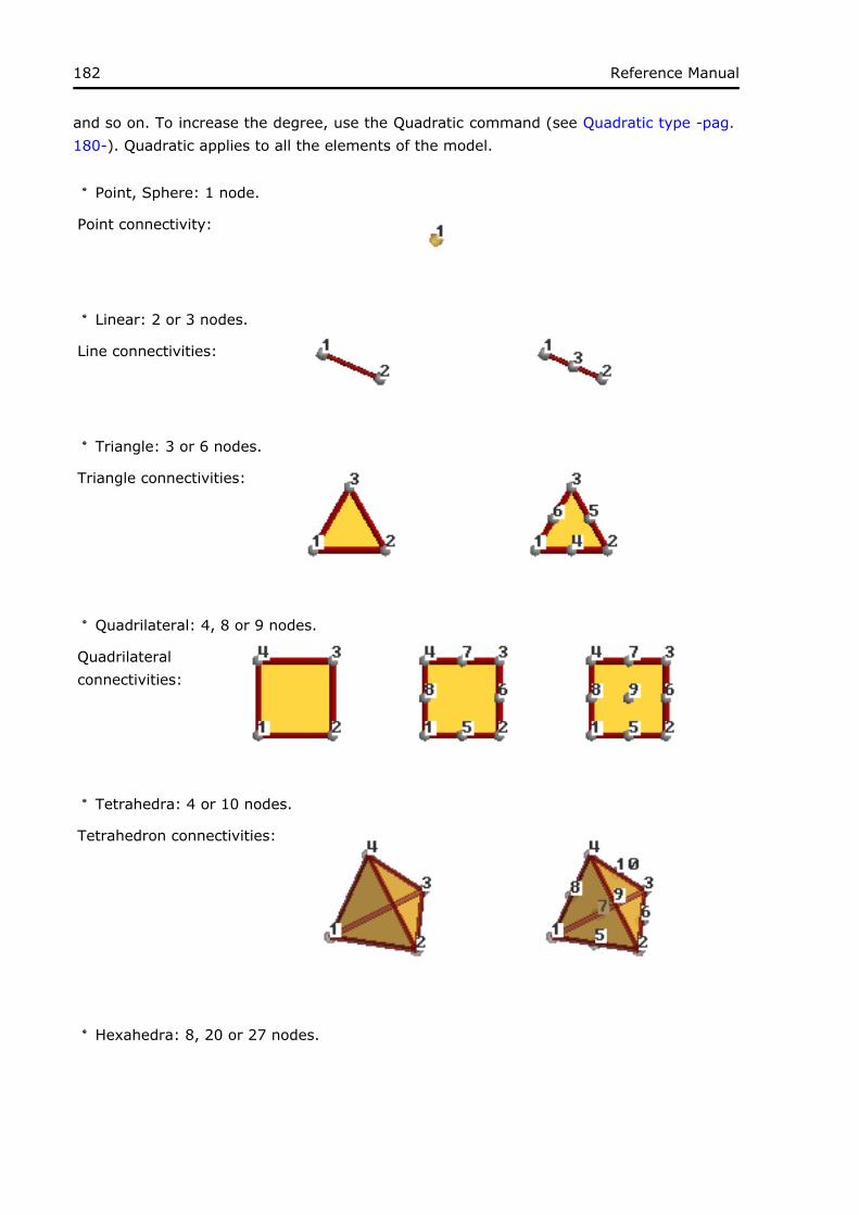
182 Reference Manual
and so on. To increase the degree, use the Quadratic command (see Quadratic type -pag. 180-). Quadratic applies to all the elements of the model.
Point, Sphere: 1 node.
Point connectivity:
Linear: 2 or 3 nodes.
Line connectivities:
Triangle: 3 or 6 nodes.
Triangle connectivities:
Quadrilateral: 4, 8 or 9 nodes.
Quadrilateral connectivities:
Tetrahedra: 4 or 10 nodes.
Tetrahedron connectivities:
Hexahedra: 8, 20 or 27 nodes.

183Element type
Hexahedron connectivities:
Prism: 6 , 15 or 18 nodes.
Prism connectivities:
Pyramid: 5 or 13 nod
Pyramid connectivities:
To see how to get information from GiD concerning element faces see Multiple values return commands from Customization Manual.
To decide which parts of the geometry should be meshed, use the Mesh criteria command (see Mesh criteria -pag. 183-).
3.3.8 Mesh criteria
Menu: Mesh->Mesh criteria
GiD provides four different criteria to generate the mesh. The Default option set all the other ones to the default value.
3.3.8.1 Mesh NoMesh

184 Reference Manual
The Mesh option lets you choose the entities to be meshed, while the No Mesh option does the opposite. By default, the No Mesh option is set.
It has to be considered that the mesh of an entity can be generated by GiD in order to generate the mesh of a higher level entity (for instance, to generate the mesh of a volume, the mesh of its surfaces is generated first). In this cases, the mesh of the lower entity (in the example, the surface one), is deleted automatically after generating the higher level one.
Some example:
If the model has one volume, and nothing is assigned (No Mesh option is set by default), after generating the mesh the user will get the tetrahedra mesh (or hexahedra), but not the surfaces meshes (triangles or quadrilateral). In order to get the surfaces meshes (which are the triangles skin of the tetrahedra), the user may set 'Mesh' option to the surfaces previously to generating the mesh.If a surface does not belong to any volume, its mesh will always appear after mesh generation, unless 'No Mesh' option has been assigned to it.Analogously, the mesh of a line will not appear if it belongs to a surface, and the 'Mesh' option has not been set explicitly to the line.
3.3.8.2 Skip
The Skip option forces GiD to skip a geometrical entity when meshing (so the entity will not have mesh), while the No Skip option forces GiD not to skip the geometrical entity (so the entity will have mesh) when the RJUMP surface mesher or Octree volume mesher is used (see Preferences -pag. 77- ). By default, any entity is skipped.
The Automatic skip option lets GiD decide if the geometrical entity should be skipped or not skipped when the RJUMP surface mesher or Octree volume one is used. This decision is taken according to the tangency between entities: those entities that are tangent enough will be skipped when meshing.
Entities with some condition or material assigned are never skipped. Entities owning to different groups are never meshed together.
Using the 'Skip by...' option user can apply some of the usefull following criteria to select the entities to be skipped, not to be skipped or to be skipped automatically.
Tangency limit angle: This criteria select the lines between surfaces in which angles between normals in the surfaces are lower than the value.Take care layers: If this is set, lines between surfaces which are in different layers won't be selected.Take care curvatures: This ratio means the diference between curvatures in the surfaces that share a line. If the ratio between the curvatures exceeds this value, the shared line is not considered to be selected. As an example, if this value is 0.1 (10%), the only lines which will be selected will be the ones in which the two surfaces that

185Skip
share the line have almost the same curvature (only a 10% of difference is accepted ). As this number increases, probably more lines will be selected. Lines of surfaces smaller than: All the lines of surfaces which have some line smaller than this value will be selected.
Window to assign skip criteria to lines.
By clicking Select by criteria all the selected criteria are used to select the lines. Modify selection allows the user to modify manually the selection made.When Apply is clicked the marked option (Skip, No skip or Automatic skip) is aplied to the selected lines.
3.3.8.3 Force points
The 'Force points to' option forces the selected points to belong to the surface or volume mesh, even though they do not necessarily belong to the surface or the volume topologically. By default no point is forced to any surface or volume mesh.

186 Reference Manual
Model of a surface and a line, with no topological relationship. Surface and line are isolated.
Mesh of the model assigning to one point of the isolated line the 'Force' option to the surface. It can be seen that the final surface
mesh contains the node corresponding to the point set.
3.3.8.4 Duplicate
Use the Duplicate option when you want to create a discontinuity in the mesh in a particular place by duplicating nodes. This is interesting, for example, when dealing with very thin shapes where it is difficult to represent the domain with two overlapped surfaces, and it is easier to have a single surface marked with this meshing option (like sails embedded in a volume, material cracks, etc.).

187Duplicate
Marked lines and the deformated mesh after an structural analysis
It is possible to mark lines embedded in a 2D domain, or surfaces in the case of 3D domains.
3.3.9 Reset mesh data
Menu: Mesh->Reset mesh data
This command resets all the meshing properties assigned to entities. These are:
Structured type (unstructured, structured, semi-structured or cartesian) Boundary layer mesh properties Element type Mesh sizes (both structured and unstructured) All the Mesh criteria (see Mesh criteria -pag. 183-).
This means that all of them will be unassigned.
To unassign properties of some specific entity, assign the corresponding 'Default' option on it. For instance, set Unstructured to an entity to reset its structured type, or set 'Default' Element type to reset the element type.
3.3.10 Draw
Menu: Mesh->Draw
This option is used to draw the meshing properties assigned to the geometrical entities.
3.3.10.1 Sizes
Menu: Mesh->Draw->Sizes

188 Reference Manual
When sizes are assigned to points, lines, surfaces or volumes using the Assign Unstruct sizes option, it is possible to draw the different assigned sizes in different colors.
EXAMPLE
In the following example some different sizes are assigned to surfaces. Sizes of 3, 5 and 6 are assigned depending on the surface.
After choosing the Draw Sizes option (over surfaces) we get the following result:
3.3.10.2 Num of divisions

189Num of divisions
Menu: Mesh->Draw->Num of divisions
With this option you can see the number of divisions assigned to the structured lines of the model (see Structured -pag. 171-).
3.3.10.3 Element type
Menu: Mesh->Draw->Element type
With this option you can see which element types have been assigned to each geometric entity. If no element type has been assigned, it is shown as Default (see Mesh Menu -pag. 167-).
3.3.10.4 Mesh - No mesh
Menu: Mesh->Draw->Mesh / No mesh
With this option you can see the entities that GiD has either been forced to mesh or forced not to mesh (see Mesh NoMesh -pag. 183-). If the meshing criteria have not been assigned to an entity, it is shown as Default (see Mesh Menu -pag. 167-).
3.3.10.5 Structured type
Menu: Mesh->Draw->Structured type
With this option you can see what kind of mesh will be generated for geometrical entities, i.e. Unstructured, Structured or Semi-structured. If no level of structure has been assigned, it is shown as Default (see Mesh Menu -pag. 167-).
3.3.10.6 Skip entities (Rjump)
Menu: Mesh->Draw->Skip entities (Rjump)
With this option you can see which lines and points will be skipped when meshing using the meshing preferences set at that moment (see Preferences -pag. 77- ), and the lines and points set as Skip or NoSkip mesh criteria (see Skip -pag. 184-).
3.3.10.7 Duplicate
Menu: Mesh->Draw->Duplicate
With this option you can see the entities that have been assigned duplicate mesh (see Duplicate -pag. 186-).
3.3.10.8 Force points to

190 Reference Manual
Menu: Mesh->Draw->Force point to
With this option you can see the number of points forced to be in the mesh of a surface or volume (see Force points -pag. 185-).
3.3.10.9 Boundary layer
Menu: Mesh->Draw->Boundary layer
With this option you can see the first layer height of the boundary layers set in the model (see Boundary layer -pag. 179-). In '2 dimensional' option the lines from wich the boundary layer will grow are shown, and in '3 dimensional' the surfaces.
In cases where two boundary layer meshes grow from the same geometrical entity (one for each side), the minimum value of the first layer heigt is shown.
3.3.11 Generate mesh
Menu: Mesh->Generate mesh...
When everything is ready for mesh generation, select this command. If there is a previously generated mesh, GiD asks if this should be erased. It will be lost from the memory, but will remain on the disk until the project is next saved (see Save (Only Preprocessing) -pag. 32-).
The meshers to be used can be chosen in preferences (see Meshing -pag. 85-).
Next, GiD asks for a general element size which will be applied to all lines, surfaces and volumes with no specific size assigned. GiD offers two default possibilities:
One default size automatically calculated by the program to define a coarse mesh.The last size given by the user in a previous meshing.
You can choose one of these or enter a new one.
The size is given by the average side of the corresponding element.
When a GiD model is saved, the meshing parameters used in the last time it was meshed are stored with the model. This parameters are the ones present in the Meshing branch of the Preferences window (Meshing -pag. 85-).
In the window appearing when you generate a mesh, he option 'Get meshing parameters from model' controls the parameters used for the meshing: if it is set, the parameters stored with the model are used, otherwise, the ones from the preferences window are considered.
During the meshing process, a progress bar indicates the number nodes and elements generated, as well as the memory consumed and the percentage done considering all the

191Generate mesh
entities to be meshed.
Meshing can be stopped at any time by clicking the Stop button. Sometimes it is necessary to press the button repeatedly or keep it pressed for a few seconds.
3.3.12 Erase mesh
Menu: Mesh->Erase mesh...
If the model has a mesh this option erases it.
3.3.13 Edit mesh
Menu: Mesh->Edit mesh
GiD offers you several options for modifying an existing mesh. All modifications will be lost when the mesh is generated again.
3.3.13.1 Create node
This tool allow the manual creation of mesh nodes, entering its x,y,z coordinates.
3.3.13.2 Move node
Menu: Mesh->Edit mesh->Move node
By using this command, an existing node is selected and moved. The new position is entered in the usual way (see Point definition -pag. 21-).
3.3.13.3 Create element
This tool allows the manual creation of mesh elements, entering its connectivities (nodes must be previously created).
For cartesian meshes, it is only needed to specify the nodes of two opposite corners. Multiple elemenst will be created to fill all cells between the two corners.
3.3.13.4 Split elements
Menu: Mesh->Edit mesh->Split elements
To split elements, select them in the usual way (see Entity selection -pag. 26-), and then press escape (see Escape -pag. 29-) to perform the action. Triangles can be split into triangles, quadrilaterals into two or four triangles, tetrahedra into tetrahedra, hexahedra

192 Reference Manual
into tetrahedra, and prisms into tetrahedra.
When splitting triangles, the new nodes can be located in the mid-edge or with an enhanced interpolation (modified Butterfly scheme) in order to obtain a smooth mesh.
When splitting quadrilaterals, if 'SymmetricalStructuredTriangles' is set (see Meshing -pag. 85-), then four triangles are generated for each quadrilateral; otherwise only two triangles are created per element.
When splitting hexahedra, if 'SymmetricalStructuredTetrahedra' is set (see Meshing -pag. 85-) , then 24 tetrahedra are generated for each hexahedron; otherwise six tetrahedra are created per element.
If original elements are quadratic, the triangles or tetrahedra obtained are quadratic. Otherwise, if original elements are linear, the triangles or tetrahedra obtained are linear.
In the case of quadratic quadrilaterals, extra nodes are generated. These nodes are not associated with geometric entities, they have simply been obtained by interpolating mesh node coordinates.
In the case of hexahedra or prisms, all selected elements must be of the same quadratic type.
With triangles or tetrahedra, when selecting only a part of the mesh, neighbor elements will be also splitted to mantain a conformal mesh. For tetrahedra is not possible to split them if they are connected with neighbor elements of another element type (to avoid create non-conformal meshes and hanging nodes)
Note: Currently, the operation Split triangles and tetrahedra only works for linear elements.
3.3.13.5 Smooth elements
Menu: Mesh->Edit mesh->Smooth elements
To smooth elements, select them in the usual way (see Entity selection -pag. 26-), and then press escape (see Escape -pag. 29-) to perform the action.
Currently only triangles, tetrahedra and hexahedra can be smoothed.
In the case of tetrahedra and hexahedra, element connectivity is preserved after the smoothing; however, with triangle elements this may be modified during the smoothing process.

193Smooth elements
In case of triangles, sharp edges can be preserved in the smoothing process. User can set the maximum angle to be considered as sharp by the 'TolAngle' option in the contextual menu (Mouse operations -pag. 18-).
All selected elements must be of the same quadratic type.
3.3.13.6 Collapse
Menu: Mesh->Edit mesh->Collapse
The Collapse function converts coincident entities, i.e. entities that are close each other, into one.
It is possible to collapse edges, nodes, elements or the whole mesh.
Collapse mesh collapses all the nodes of the mesh.Collapse edges joins nodes that are connected by edges shorter than the Import Tolerance value.Collapse nodes asks you to select some nodes. Nodes closer together than the Import Tolerance value are collapsed.Collapse elements asks you to select some elements. Then, the nodes of these elements that are closer together than the Import Tolerance value are collapsed.
Note: Entities belonging to a frozen layer (see Layers and groups (only Preprocessing) -pag. 98-) are not checked when collapsing.
3.3.13.7 Delete
Menu: Mesh->Edit mesh->Delete
To delete elements or nodes, select them in the usual way (see Entity selection -pag. 26- ), and then press escape (see Escape -pag. 29- ) to perform the action.
Nodes that no longer belong to any element after the operation are also erased.
Note: It is possible to filter the selection, e.g. to select only triangles but not quadrilaterals (see Selection window (only Preprocessing) -pag. 109- ).
Note: Only lonely nodes (nodes of the mesh that do not belong to any element) can be deleted.
3.3.14 Show errors
Menu: Mesh->Show errors...
This option opens the mesh errors window, which is automatically opened just after the

194 Reference Manual
meshing process, if some entity could not be meshed. This window presents a list of the entities that GiD could not mesh, and some information about the problems that occurred during the meshing process. By right-clicking over an item in the list, advice will be displayed about how to solve the meshing problems for each geometrical entity.
3.3.15 View mesh boundary
Menu: Mesh->View mesh boundary
This option draws the boundaries of the mesh on the screen. The resulting mesh is not stored, it is just for visualization purposes.
Boundaries for triangular or quadrilateral meshes are line elements.
Boundaries for tetrahedra or brick meshes are triangles or quadrilaterals. This option can be useful when rendering a volume mesh (see Render -pag. 62-).
3.3.16 Create boundary mesh
Menu: Mesh->Create boundary mesh
This option creates the boundary mesh of the existing mesh.
The boundary mesh for triangular or quadrilateral meshes is a line element mesh.
The boundary mesh for tetrahedra or brick meshes is a triangular or quadrilateral mesh.
3.3.17 Mesh quality
Menu: Mesh->Mesh quality
This option opens a window that shows information about the quality of the mesh elements.

195Mesh quality
Mesh Quality window
There are ten criteria used to measure the quality of the elements, or to provide with some measure of the mesh:
1 Minimum angle: The quality criterion is the minimum angle in surface elements and the minimum dihedral angle for volume elements. This means that elements with a small angle are considered to be of a worse quality than ones with bigger angles.
2 Maximum angle: This gives the maximum angle for every element. Elements with bigger angles are considered worse. Typically, the Minimum angle criterion is good for qualifying triangles and tetrahedra and the Maximum angle criterion is good for quadrilaterals and hexahedra
3 Element vol: The quality criterion is the size of elements (distance for lines, area for surfaces and volume for volumes). Elements with small "volume" are considered worse.
4 Minimum edge: The quality criterion is the size of the smaller edge of each element. Elements with smaller edges are considered worse.
5 Maximum edge: The quality criterion is the size of the largest edge of each element. Elements with bigger edges are considered worse.
6 Shape quality: The quality criterion measures the likeness of the element to the reference one (an equilateral triangle in the case of triangles, a regular tetrahedron in the case of tetrahedra, a square in the case of quadrilaterals and a cube in the case of hexahedra). Its value is 1 for a perfect element (the reference one), and it decreases as the element becomes worse. If it reaches a negative figure it means that the element has a negative Jacobian at some point. The mathematical expression of this quality measure for each type of element is as follows.
Triangles: The shape quality (q) of triangles is measured as

196 Reference Manual
where Area is the area of the triangle, and l_i (i=1..3) are the lengths of the triangle's edges.
Tetrahedra: The shape quality (q) of tetrahedra is measured as
where Volume is the volume of the tetrahedron, and l_i (i=1..6) are the lengths of the tetrahedron's edges.
Quadrilaterals: The shape quality (q) of quadrilaterals is measured as the quality of the worst quality node. The quality of a node (q_n) is given by
where l_1 and l_2 are the lengths of concurrent edges of the node, and Area_n is the area of a fictitious parallelogram, made with these two edges.
Hexahedra: The shape quality (q) of hexahedra is measured as the quality of the worst quality node. The quality of a node (q_n) is given by
where l_1, l_2, l_3, A_1, A_2, A_3 are the lengths and areas of concurrent edges and faces of the node, and Volume_n is the volume of a fictitious parallelepiped, made with these concurrent faces.
7 Minimum Jacobian: The quality criterion is the value of the minimum Jacobian between the Jacobians calculated at each element Gauss point. If there are elements with negative Jacobians, problems may be encoutered in some calculation processes.
8 Radius: This option is only available for sphere and circle elements. It represents the radius of the element.
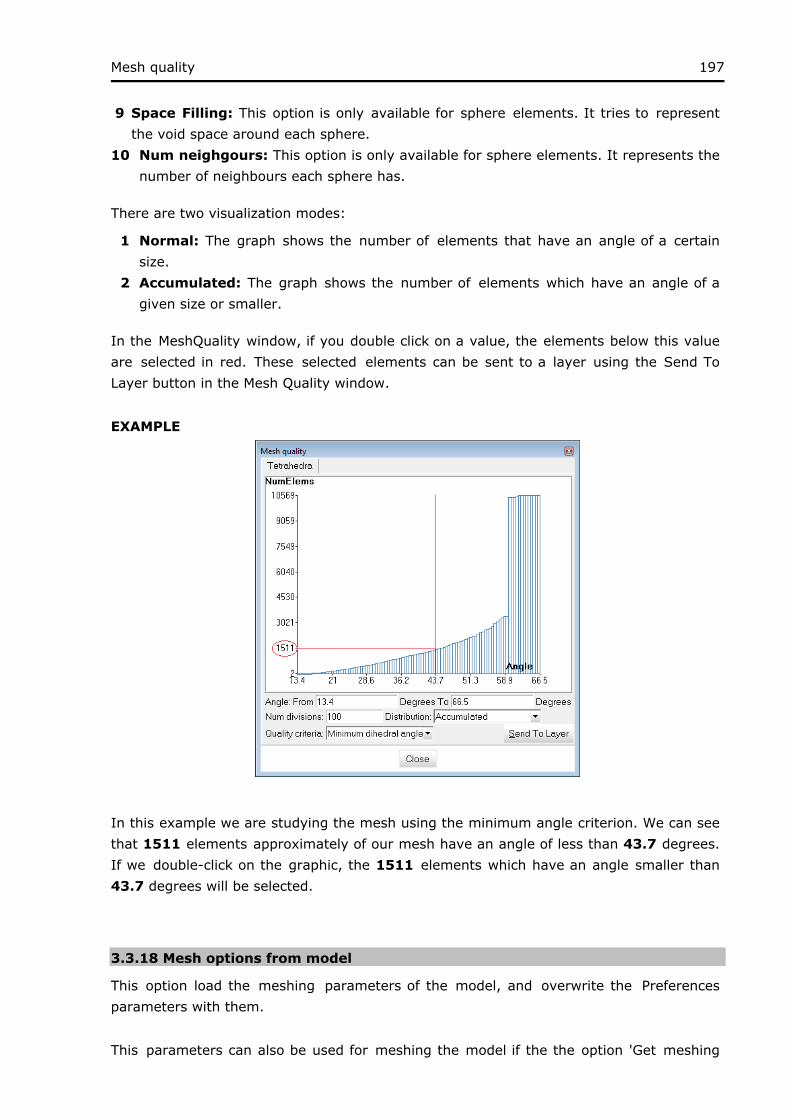
197Mesh quality
9 Space Filling: This option is only available for sphere elements. It tries to represent the void space around each sphere.
10 Num neighgours: This option is only available for sphere elements. It represents the number of neighbours each sphere has.
There are two visualization modes:
1 Normal: The graph shows the number of elements that have an angle of a certain size.
2 Accumulated: The graph shows the number of elements which have an angle of a given size or smaller.
In the MeshQuality window, if you double click on a value, the elements below this value are selected in red. These selected elements can be sent to a layer using the Send To Layer button in the Mesh Quality window.
EXAMPLE
In this example we are studying the mesh using the minimum angle criterion. We can see that 1511 elements approximately of our mesh have an angle of less than 43.7 degrees. If we double-click on the graphic, the 1511 elements which have an angle smaller than 43.7 degrees will be selected.
3.3.18 Mesh options from model
This option load the meshing parameters of the model, and overwrite the Preferences parameters with them.
This parameters can also be used for meshing the model if the the option 'Get meshing

198 Reference Manual
parameters from model' is set in the appearing window when 'Mesh->Generate mesh' is set (see Generate mesh -pag. 190-).
3.4 Calculate Menu
With this menu, you can initiate and manage the analysis of a problem. hereafter referred to as a "process". You will see in the sections that follow that several analyses, or processes, can be run at the same time.
3.4.1 Calculate
Menu: Calculate->Calculate
This option begins the process module. Once it is selected, you can continue working with GiD as usual.
3.4.2 Calculate remote
Menu: Calculate->Calculate remote
This option begins the process module on a remote machine. Once it is selected, you can continue working with GiD as usual.
Note: ProcServer with the same model problem type must be installed and running on the remote machine in order to use this option. (ProcServer is not included by default with GiD, but it could be download from its web page)
3.4.3 Cancel process
Menu: Calculate->Cancel process
Selecting a proces that is currently running and clicking this option will halt its execution.
3.4.4 View process info
Menu: Calculate->Viewprocess info...
Select a process that is currently running and click this option to open a window that shows information relating to the process, such as iterations, convergence, etc. Clicking Close will close the window, but will not halt the process.
3.4.5 Calculate window
Menu: Calculate->Calculate window...

199Calculate window
Selecting this option opens a window in which a list of all the running processes is shown, along with some useful information like name, starting time, etc.
Process window
The buttons in this window let you control some running process features, such as terminating the process (Terminate), starting a remote calculation (Start remote), or setting remote analysis properties (Remote...). These remote analysis properties are shown in the next figure.
Window to customize remote calculation options.

200 Reference Manual
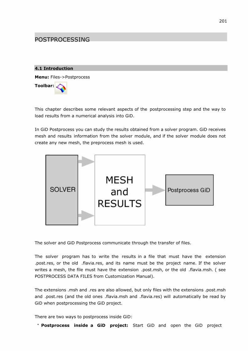
POSTPROCESSING
201
4.1 Introduction
Menu: Files->Postprocess
Toolbar:
This chapter describes some relevant aspects of the postprocessing step and the way to load results from a numerical analysis into GiD.
In GiD Postprocess you can study the results obtained from a solver program. GiD receives mesh and results information from the solver module, and if the solver module does not create any new mesh, the preprocess mesh is used.
The solver and GiD Postprocess communicate through the transfer of files.
The solver program has to write the results in a file that must have the extension .post.res, or the old .flavia.res, and its name must be the project name. If the solver writes a mesh, the file must have the extension .post.msh, or the old .flavia.msh. ( see POSTPROCESS DATA FILES from Customization Manual).
The extensions .msh and .res are also allowed, but only files with the extensions .post.msh and .post.res (and the old ones .flavia.msh and .flavia.res) will automatically be read by GiD when postprocessing the GiD project.
There are two ways to postprocess inside GiD:
Postprocess inside a GiD project: Start GiD and open the GiD project

202 Reference Manual
(ProjectName.gid) you want to postprocess, and then select the Postprocess option from the files menu or click on the pre/post toolbar button. This way the file ProjectName.post.res, or the old ProjectName.flavia.res, will automatically be read by GiD, along with the file ProjectName.post.msh, or ProjectName.flavia.msh, if present.Postprocess other files: Start GiD and select the Postprocess option directly from the files menu or click on the pre/post toolbar button. Now open the pair files OtherModel.msh and OtherModel.res.
A list of the supported elements and results can be found on Postprocess mesh format: ProjectName.post.msh from Customization Manual.
Once inside the postprocessing component of GiD, all the visualization features and management options of the preprocessing section are available: Zoom, Rotate (Rotate screen/object axes, Rotate trackball,etc.), Pan, Redraw, Render, Label, Clip Planes, Perspective, etc.
Note: There is no need to load a project into GiD to use its postprocessing facility; you can open mesh and results information directly from GiD Postprocess (see Files Menu -pag. 29-).
4.2 Do Cuts Menu
Menu: Do cuts
Here you can cut and divide volumes, surfaces and transform cuts into true meshes. A cut of a volume mesh results in a cut plane. The cut is done for all the meshes, even those that are switched Off. When cutting surfaces, a line set will be created. Here only those surfaces that are switched On are cut.
The difference between cut meshes and surface or volume meshes is that only the mesh is stored in memory, together with some interpolation information, and each time the user selects a result to visualize, this result is interpolated to the cut mesh, saving memory space. When the user converts cuts to surface meshes, then all results of the analysis are interpolated for the transformed cut meshes and stored in memory.
Saving a cut mesh, merelly saves the cut plane, or spere, used to create it. But saving a converted cut mesh will save a true mesh with the results interpolated over it.
Another feature is that a cut can be deformed, if meshes are also told to do so (see Deformation -pag. 223-). A cut of a deformed mesh, when changing to the original shape, will be deformed accordingly.
When dividing volumes/surfaces, only those elements of the volumes/surfaces that are switched On and which lie on one side of a specified plane will be used to create another volume/surface.

203Do Cuts Menu
Several dividing options can be found by right clicking on the graphical screen when the options 'cut' or 'divide' are selected.
Cutting spheres will result in a mesh of circles.
Toolbar:
Do cut plane:
2 Points
3 Points
Succession
Cut Plane: Specify a plane which cuts the volumes/surfaces. Several options can be used to enter this plane.
2 Points: the plane is defined by two points and the visual direction orthogonal to the screen. 3 Points: the plane is defined by three points. When choosing the points, the nodes of the mesh can also be used. Succession: This option is an enhancement of Cut Plane. Here you specify an axis that will be used to create cut planes orthogonal to this axis. The number of planes is also asked for.
Divide by selection: After selecting some elements, they will be removed from their original mesh sent to a new mesh.Divide Volume Sets: Specify a plane which is used to divide the meshes. Several options can be used to enter this plane. With Two Points (the default), the plane is defined by the corresponding line and the direction orthogonal the screen. With Three Points, the plane is defined by three points. When choosing the points, the nodes of the mesh can also be used. After defining the plane, you should choose which section of the mesh should be saved by selecting the side of the plane to use. Only those elements that lie entirely on this side are selected. Only those volume meshes that are shown are divided.Divide Surface Sets: Specify a plane which is used to divide the sets. Several options can be used to enter this plane. With Two Points (the default), the plane is defined by the corresponding line and the direction orthogonal to the screen. With Three Points, the plane is defined by three points. When choosing the points, the nodes of the mesh can also be used. After defining the plane, you should choose which section of the mesh should be saved by selecting the side of the plane to use. Only those elements that lie entirely on this side are selected. Only those surface meshes that are shown are divided. When doing a division, there are several useful options inside the Contextual mouse menu (right-click in the graphical window):
exact: to do an exact division, i.e. elements are cut to create the division;parallel planes: the remaining elements will be the ones between two parallel planes.

204 Reference Manual
A distance can also be entered, after choosing this option from the Contextual menu.
Divide lines: Specify a plane which is used to get the lines on one side of this plane2D polygonal cut: Here you can define a polygonal on the screen. This polygonal is then used to cut the triangular and quadrilateral meshes to create a cut mesh of lines. So when the surfaces are deformed, the polygonal cut is deformed too. And vice versa, if a polygonal cut is defined while the surfaces are deformed, when turning them into its original shape, the polygonal cut is "undeformed" with them. These cuts can be imported and exported and are saved between sessions, like normal cut planes. Quadratic elements are handled as linear ones, like normal cut planes. Nodal results and 1gp results are passed to the new cuts as well.Cut Spheres: Here you can define a sphere which will be used to cut the volume and surface meshes, resulting in triangle or line cut meshes respectively.Convert cuts to surface sets: With this options cuts can be converted to surface sets so they can be saved, or cut again.Automatically convert cut to set: It this options is selected, cuts are automatically converted to sets (some operations are available for sets but not for cuts)
Cuts can also be read from and written to a file. The information stored to the file from a 'Cut Plane' is the plane equation that defines the plane ( Ax + By + Cz + D = 0), so it can be used with several models. The information stored in the file from a 'Cut Wire' is the points list of the cut-wire, i.e. the intersection between the wire and the edges of the meshes/sets. These files are standard ASCII files. A line of a 'Cut Plane' archive contains the four coefficients of the plane that defines the cut, separated by spaces. A line of a 'Cut Wire' archive contains the three coordinates of a point of the wire. Comment lines are allowed and should begin with a '#'.
An example of a 'Cut Plane' file where three planes were written:
# planes created from a 'cut succession' -10.82439 0.5740206 0 51.62557 -10.82439 0.5740206 0 12.45994 -10.82439 0.5740206 0 -26.70569
An example of a '2D polygonal cut' file:
-2.444425 3.883427 2.487002 2.130787 2.762815 3.885021 0.8411534 4.458836 3.215301 4.270067 3.795048 2.037187 5.66561 3.414776 0.8219391 2.945865 3.600701 3.29012

205Do Cuts Menu
0.4487007 3.764661 3.574121
4.3 View Results Menu
The kinds of results that will be displayed on screen can be grouped into five major categories:
Scalar view results: Show Minimum & Maximum, Contour Fill, Contour Text Ranges, Contour Lines, Iso Surface, Result surface, Line thickness and their configuration options.Vector view results: Mesh deformation, Display Vectors, Stream Lines, Node traceLine diagrams: Scalar line diagram and vector diagrams.Graph lines: XY plots, polar plots.Animation: Animation of the current results visualizations.
The View Results menu and window are used to manage the visualization of the different type of results.
Menu: View results
The View Results menu lets you select any type of result:
Contour fillContour linesContour rangesShow min/maxDisplay vectorsIso surfacesStream linesNode traceGraphsResult surfaceDeformationLine diagramLine thicknessIntegrateDistribution...
Smoothed sub-menu with gaussian results:
Results can be located on the nodes of the mesh, nodal results, or on the integration points defined on the elements, known as gauss points, gaussian results.

206 Reference Manual
For instance, selecting a contour fill visualization of a nodal result will draw a continous colour map over the mesh geometry. But for results located at the gauss points, there is no guarantee that the values are continous between elements; in fact they are usually discontinous. So, visualizing a Contour fill of a gaussian result will display a discontinuous colour map over the mesh:
Contour fill of a nodal result Contour fill of a gaussian result
Most of the above results visualization can be performed over nodal and gaussian results. Currently the exceptions are: Contour text ranges, Stream lines, node trace, graphs, and deformations.
GiD also smoothes the gaussian results to provide a continous colour map:
Contour fill of a gaussian result Contour fill of the same gaussian result but globally smoothed
How the global smoothing is done can be adjusted with Options --> Contour --> Smoothing type:
Minimum value: The minimum value between two adjacent elements is the result that is used.Maximum value: The maximum value between two adjacent elements is the result that is used.Mean value: A mean value of the points between two adjacent elements is the result that is used.

207View Results Menu
If there are gaussian results present in the simulation files, and if these gaussian results can be smoothed, then in the results visualizations menus, besides the results list a new entry will appear with the label Smoothed, and a sub-menu will pop-up with the gaussian results which can be globally smoothed:
Added sub-menu to perform a result's visualization with gaussian results globally smoothed
Following results visualizations can be performed on smoothed gaussian results:
Contour Fill, Contour lines, Iso surfaces, Graphs, Result surfaces and Line thickness
Menu: Window->View results
The View Results window manages the visualization of the following type of results:
Contour fillSmooth contour fill ( of gaussian results globally smoothed), same as the menu Contour fill --> SmoothedContour ranges (if Result Range Tables are present)Contour linesSmooth contour lines ( of gaussian results globally smoothed), same as the menu Contour lines --> SmoothedDisplay vectorsShow min/maxResult surfaceSmooth result surface ( of gaussian results globally smoothed), same as the menu Result surface --> SmoothedLine thicknessSmooth line thickness ( of gaussian results globally smoothed), same as the menu Line thickness --> Smoothed

208 Reference Manual
Scalar and Vector line diagram (if Linear elements are present)
View Results window
As the results are grouped into steps and analyses, GiD must know which analysis and step is currently selected for displaying results. The Analysis menu of the View Results window is used to select the current analysis and step to be used for the rest of the results options. If some of the results view requires another analysis or step, you will be asked for it.
Note: If you no longer wish to view results, you can select No Result in this window or in the View results menu.
4.3.1 No Results
Menu: View results->No results
Toolbar:
4.3.2 No Graphs
Menu: View results->No Graphs
Toolbar:

209Default Analysis - Step
4.3.3 Default Analysis - Step
Menu: View results->Default Analysis/Step
Toolbar:
4.3.4 Contour Fill
Menu: View results->Contour Fill
Toolbar:
This option allows the visualization of colored zones, in which a variable or a component varies between two defined values. GiD can use as many colors as permitted by the graphical capabilities of the computer. When a high number of colors is used, the variation of these colors looks continuous, but the visualization becomes slower unless the Fast-Rotation option is used. A menu of the variables to be represented will be shown, and the one that is chosen will be displayed using the default analysis and step selected.
Vectors will be unfolded into their X, Y, and Z components and module. Symmetrical matrix values will be unfolded into the Sxx component, Syy component, Szz component, Sxy component, Syz component and Sxz component of the original matrix and also into the Si component, Sii component and Siii component in 3D problems or angular variation in 2D problems. Any of these components can be selected to be visualized.
Contour fill is supported for results defined over nodes or gauss points.
If the gauss points results can be globally smoothed, then a Smoothed sub-menu will be added with a list of the gaussian results, see View Results Menu -pag. 205-
When using results defined over gauss points, they are extrapolated to the nodes so that discontinuities can appear between adjacent elements. If the gauss points results cannot be extrapolated to the nodes, they are drawn as coloured spheres. The radius and detail level of these spheres can be configured as well (see Point options -pag. 229- ).
Several configuration options can be accessed via the Options menu.
Menu: Options->Contour
Toolbar:
Set maximum value

210 Reference Manual
Set minimum value
Contour options
Scale result->Use logarithmic scale
Scale result->Multiplier factor
Scale result->Added factor
Reset Limit Values
Number of Colors: Here the number of colors of the results color ramp can be specified. Width Intervals: Fixes the width of each color zone. For instance, if a width interval of 2 is set, each color will represent a zone where the results differ by two units at the most. Set Limits: This option is used to tell the program which contour limits it should use when there are no user defined limits: the absolute minimum and maximum of all sets or shown sets, for the actual step or for all steps. Define limits: When choosing this option the Contour Limits window appears (this option is also available in the Postprocess toolbar). With this window you can set the minimum/maximum value that Contour Fill should use. Outliers will be drawn in the color defined in the Out Min Color/Out Max Color option. Reset Limit Values: This option resets the values defined in the Define limits option. Reset All: This option sets all Contour Fill options by default. Max/Min Options: Inside this group, several options for the minimum or maximum value can be defined:
ResetValue: Here you can reset the maximum/minimum value, so that the default value is used. Out Max Color / Out Min Color: With this option you can specify how the outlying values should be drawn: Black, White, Max/Min Color, Transparent or Material. Def. Max Color / Def. Min Color: This option lets you define the color for the minimum or maximum value for the color scale to start with. Set Value: This option allows the user to fix a Maximum or Minimum limit for the color scale.
Color scale: Specifies the properties of the color scale: Standard: The color scale will be the default: starting from blue (minimum) through green to red (maximum). Inverse Standard: The color scale will be the inverse of the default: starting from red (minimum) through green to blue (maximum).

211Contour Fill
Terrain Map: A physical map-like color ramp will be used. Black White: Black for Minimum and White for Maximum, and a grey scale between these. White Black: White for Minimum and White for Maximum, and a grey scale between these. 3D anaglyphs: Colour scale specially useful when the software stereo mode is enabled. Advanced viewing settings -pag. 66-3D anaglyphs 2: A variation of 3D anaglyphs.User defined: The color scale can be fully set by user. (See color window).Scale Ramp: This option lets user specify how the ramp should change from minimum color to the maximum color: Tangent, ArcTangent or Linear. The default is ArcTangent.Scale Type: Tells GiD how the colors between the minimum color and the maximum color should change: RGB or HSV.
Smoothing type: With this option you can choose between these types of local smoothing:
Minimum value: The minimum value between two adjacent elements is the result that is used.Maximum value: The maximum value between two adjacent elements is the result that is used.Mean value: ( the default) A mean value of the points between two adjacent elements is the result that is used.
Bright color: Enables or disables the shininess of the colours in Contour Fill. The shininess type can also be choosed between: metallic, plastic and rubber. Color window: A window opens to let you configure the colour scale of the contours easily.

212 Reference Manual
Scale result: Use logarithmic scale, multiplier factor and added factor
4.3.5 Contour Lines
Menu: View results->Contour Lines
Toolbar:
This display option is quite similar to Contour Fill (see Contour Fill -pag. 209-), but here the isolines of a certain nodal variable are drawn. In this case, each color ties several points with the same value of the variable chosen.
Here the configuration options are almost the same as the ones for Contour Fill (see Contour Fill -pag. 209-), with the only difference being that the number given in the Number of Colors option will be used as the number of lines for this contour lines representation.
Contour lines are supported for results defined over nodes or gauss points.
If the gauss points results can be globally smoothed, then a Smoothed sub-menu will be added with a list of the gaussian results, see View Results Menu -pag. 205-
The width of the contour lines can be adjusted with Options --> Contour --> Lines width .
4.3.6 Contour Ranges
Menu: View results->Contour ranges
This is the same as the Contour Fill visualization type, but the coloured areas are created following a 'Result range table' specified in the results file (see Result Range Table from Customization Manual), and the names of these areas are visualized as text labels.
Contour ranges is supported for results defined over nodes or gauss points.

213Contour Ranges
4.3.7 Show Minimum and Maximum
Menu: View results->Show Min Max
Toolbar:
Show min/max
Show minimum
Show maximum
Show both
With this option you can see the minimum and maximum of the chosen result.
Show mix max is supported for results defined over nodes or gauss points.
Note: This minimum and maximum can be absolute - for all the meshes/sets/cuts - or relative (local) to the ones displayed. This can be selected from the pull-down menu Options -> Contour -> Set Limits.
4.3.8 Display Vectors
Menu: View results->Display Vectors

214 Reference Manual
Toolbar:
This option displays a menu with results from vectors and matrices (where the principal values have been previously evaluated by the program). From the menu of variables, choose the one you wish to see displayed; it will be shown with the default analysis and step (this can be changed with the Default Analysis/Step option in the menu). Once a result is chosen, the program will display the nodal vectors of the chosen result. The vectors that are drawn can be scaled interactively. The factor can be applied several times and every time it changes to the new input value.
You can modify the colour of the vectors, which by default are drawn in green, so that all the vectors are drawn in the same colour, or you can let the color of the vectors vary according to the result module.
When drawing a matrix result (3x3 symmetrical), such as the stress tensor, only a single color representation of principal values is available: blue when negative (also drawn as >< representing compressions), and red when positive (also drawn as <> representing tensions).
A vector will be separated into its X, Y, and Z components and its module. So either the X, Y or Z component or the whole vector (represented by the module) can be drawn. Symmetrical matrices will be unfolded into: Si component, Sii component, Siii component, and 'All' components. Any of these components can be selected to be visualized. Si, Sii and Siii represent the eigen values and vectors of the matrix results which are calculated by GiD, and which are ordered according to the eigen value.
Local axes can also be drawn by means of their Euler angles.
Display vectors is supported for results defined over nodes or gauss points.
For ComplexVectors, their real part or their imaginary part can be selected to be drawn. If the modulus of the whole vector is selected, then both parts are drawn simultaneously.
Several configuration options can be accessed via the Options menu.
Menu: Options->Vectors
Interior/All vectors: This option lets you choose if all vectors should be drawn or draw only the ones placed on model lines.Number of Colors: If you use Color Modules to draw vectors, it is possible to choose the number of colors. Color Mode: This option lets you choose if vectors are drawn in one color (Mono Color) or in several colors (Color Modules). Offset: With this option, you control where the vector should be in relation of the node,

215Display Vectors
ranging from 0, to tie the tail of the arrow to the node, to 1, to tie the tip of the arrow to the node. Change Color (mono): When vectors are drawn in (Mono Color) Color Mode, they are drawn in green. You can change this green color selecting this entry.
Note: The above four options have no effect when viewing a matrix result or local axes.
Detail: The level of detail can be adjusted to draw the vectors quicker or nicer. The different options are:
No arrow head: the arrow head will not be drawn.Point: the arrow head will be drawn as a point. The style used to draw these point like arrow heads can be modified through the point options window described before, see Point options -pag. 229-. Lines: the arrow head will be drawn as four lines.2 Triangles: the arrow head will be drawn with two intersecting triangles.4 Triangles: the arrow head will be drawn as cones of four triangles.8 Triangles: the arrow head will be drawn as cones of eight triangles.
Size: Allows the user to set the size of the vectors to be: Fixed sized: Then the factor used when the vectors are displayed is the number of pixels of the vector. Modulus dependent: Then the factor used when the vectors are displayed is the factor of magnification of the vector.
Filter factor: The displayed amount of vectors can be limited when there are lots of vectors to be drawn, for instance, when very dense meshes are used. The option allows to drawn only one vector of every N vectors. This 'N' can be customized by the user in the right buttons menu, under Results --> Options --> VectorFilterFactor
Note: This last option affects also matrix and local axes results.
The displayed amount of vectors can also be limited when there are lots of vectors to be drawn, for instance, when very dense meshes are used. The option allows to drawn only one vector of every N vectors. This 'N' can be customized by the user in the right buttons menu , under Results --> Options --> VectorFilterFactor .
4.3.9 Iso Surfaces
Menu: View results->Iso Surfaces
Toolbar:
Here a surface is drawn that ties a fixed value inside a volume mesh; for surface meshes a line is drawn. To create isosurfaces there are several options:
Exact: After choosing a result or a result component of the current analysis and step,
216 Reference Manual
you can input several fixed values and then for each given value an isosurface is drawn. Automatic: Similarly, after choosing a result or a result component, you are asked for the number of isosurfaces to be created. GiD calculates the values between the Minimum and the Maximum (these are not included). Automatic Width: After choosing a result or result component, you are asked for a width. This width is used to create as many isosurfaces as are needed between the Minimum and Maximum defined values (these are included).
Iso lines are created for triangles and quadrilaterals when the isosurface visualization is selected. Their visualization can be enabled or disabled with Options --> Iso-surfaces --> Show isolines
Iso surfaces are supported for results defined over nodes or gauss points.
If the gauss points results can be globally smoothed, then a Smoothed sub-menu will be added with a list of the gaussian results, see View Results Menu -pag. 205-
Several configuration options can be accessed via the Options menu. These isolines can be switched on and off with the command Results --> IsoSurfaces --> DysplayStyle --> ShowIsolines on the right buttons menu .
Menu: Options->Iso Surfaces
Display Style: For isosurfaces there is also a Display Style option, like for Volumes/Surfaces/Cuts. The available options are: All Lines, Hidden Lines, Body, Body Lines (see View style -pag. 234- ). Transparency: The isosurfaces can be set to Transparent or Opaque (see View style -pag. 234-). Color Mode: Allows the user to define the colours used to paint the iso surfaces:
Monochrome: All the isosurfaces are drawn with the same colour, which can be adjusted with 'Change colour'. Result color: Each isosurface is drawn with a colour indicating its value, the correspondence of which can be seen in the legend. Contour Fill color: The isosurfaces are drawn with the colour scale of the current contour fill, i.e., the current contour fill is also drawn over the isosurfaces. If no contour fill is displayed, then the monochrome colour is used.
Change color: Allows to define the dolour of the monochrome isosurfaces, including the transparency factor.Convert to cuts: With this options all the isosurfaces drawn will be turned into cut meshes, so that they can be saved, read, and have results drawn over them. Results are interpolated over cut meshes on demand. To save a full-featured iso-surface with all the results of the analysis interpolated on the isosurface, first they have to be converted to cut, and then Do Cuts --> Convert cuts to surface mesh, see Do Cuts Menu -pag. 202-.Draw always: With this option the isosurfaces will be drawn although the mesh is switched off.
217Iso Surfaces
Show isolines: When the isosurface result option is selected, the isosurfaces of volume meshes are created ans isolines for surface meshes. With this option "Show isolines" the user can switch these isolines on or off.
These options also are used for isolines.
4.3.10 Stream Lines
Menu: Vies results->Stream lines
Toolbar:
With this option you can display a stream line, or in fluid dynamics, a particle tracing, in a vector field. After choosing a vector result, using the default analysis and step selected, the program asks you for a point from which to start plotting the stream line. This point can be given in several ways:
The best way to choose initial points for the stream lines is to cut the mesh through the place where the user wants the stream lines, and then select the nodes of this cut.
Clicking on the screen: The point will be the intersection between the line orthogonal to the screen and the plane parallel to the screen and containing the center of rotation. Joining a node: The selected node will be used as a start point. Selecting nodes: Here several nodes can be selected to start with. Along a line: With this option you can define a segment along which several start points will be chosen. The number of points will also be asked for, including the ends of the segment. In the case of just one start point, this will be the center of the segment. In a quad: Here you can enter four lines that define a quadrilateral area which will be used to create a N x M matrix of points. These points will be the start for the stream lines. When giving N x M, N lies on the first and third line, and M on the second and fourth. So, points (0, 0..N), (M, 0..N), (0..M, 0) and (0..M, N) will lie on the lines. But in case of N=1 or M=1, this will be the center of the line, and if N = 1 and M = 1, this will be the center of the Quad. Intersect set: The point will be the intersection between the line orthogonal to the screen and the current viewed sets nearest the viewpoint.
When creating a stream line, the user can tell GiD to create a stream line 2D constraint, by selecting this option of the right mouse button contextual menu. Then the stream line algorithm will discard the z coordinate of the meshes and of the vector field.
When viewing Stream Lines, labels can be drawn to show the times at the start and end points of the stream line.

218 Reference Manual
Stream lines can also be deleted and their color changed (green by default).
Stream lines are supported for results defined over nodes.
The there are complex vectors, the user can select between the real part ( field) of the complex vector and the imaginary part ( field).
The following options can be chosen for Stream Lines:
Menu: Options->Stream Lines
Change color: Allows the definition of the colour of the monochrome stream lines. Color Mode: Allows the user to define the colours used to paint the iso surfaces:
Monochrome: All the stream lines are drawn with the same colour, which can be adjusted with 'Change color'. Stream contour filled: The colour of the streamlines changes, ala Contour Fill acording to the modulus of the vector used to create the dtream line. Result contour filled: The stream lines are drawn with the colour scale of the current contour fill, i.e., the current contour fill is also drawn over the stream lines. If no contour fill is displayed, then the monochrome colour is used.
Delete: This option lets you select the stream lines to be deleted. Delete all: This options delete all stream lines of the model. Label: This option lets you select the kind of label:
None: No labels are drawn. 0_End: Labels are drawn according to the following convention: 0 at the start of the stream line, and the total time taken for the particle to travel at the end. Ini_End: Labels are drawn according to the following convention: 0 at the chosen point, with - time before at the beginning of the stream line and + time after at the end.
Size, colour & detail : Here you can adjust the size, width and detail of the stream lines, together with the colour options, using the Stream line options window:

219Stream Lines
Stream line options...
The type of stream can be:
points: showing the points calculated for the stream lines and used to draw them. ribbons: stream ribbons showing the swirl of the velocitys field. 4 sided prisms: stream 'tubes' with constant width.
Set initial step: 0 for automatic step. Set max length: To avoid infinite curves (e.g. in vortex). Set max points: To avoid curves with excessive (and memory expensive) number of points. Set initial rotation: Sets the initial rotation of the stream ribbons at the selected nodes. Show arrows: With this option Gid draws arrows on the stream lines showing the sense of them.
4.3.11 Node trace
This option allows the user to track nodes, whose traces are displayed. For a single mesh for the whole analysis, the node will follow the path of the deformed mesh across all steps. When several meshes are used for several time steps, then the nodes can follow the track of the original mesh or from the deformed one.

220 Reference Manual
4.3.12 Graphs
Menu: View results->Graphs
Toolbar:
Point evolution
Line graph
Point graph
Border graph
Integrate
Point complex evolution
Clear
From this menu several graphs types can be created and deleted. Graphs are supported for results defined over nodes.
Check also the view graph window where graphs can be created, customized and deleted (see View graphs -pag. 241-)
Graphs are organized into graph sets in order to ease the management. Each set shares the same units for each axis.
When a graph is created is placed in the current graphset if the units are the same,

221Graphs
otherwise a new graphset is created. To change the current graph set please use the graphs window (see View graphs -pag. 241-)
Several graph types are available:
Clear: delete all the created graphs.Point evolution: displays a graph of the evolution of the selected result along all the steps, of the default analysis, for the selected nodes.Point graph: displays a graph of one result against another of the selected results. The option 'all steps' shows the evolution along all steps inside the default analysis, of this result vs. results graph.Border graph: displays a graph of the results on the selected border, using the x, y, z or line distance as abscissa.Line graph: also called 'section graph' displays a graph defined by the line conectig two selected nodes of surfaces or volumes, or any arbitrary points on any projectable surface and in any position.Integrate: graph of an integrated result over a mesh.Point complex evolution: similar to 'Point Evolution' but for complex results, where both real and imaginary part of the result are displayed as 'x' and 'y' in the graph.
User can also save or read a graph (see Files Menu -pag. 29-).
Menu: Options->Graphs
All the following options are applied to the graphs placed in current graphset.
Coordinate type: Changes the type of graph coordinates betwee cartesian and polar.Outline on model: Shows in the model where the line and border graphs are drawn.Grids: Tell GiD whether or not to draw grids.Current style: Choose what the new graphs should look like. The possible styles are: Dot, Line, and Dot-Line.Change style graph: Changes the style of the selected graph.Change color graph: Changes the colour of the selected graph.Set contour fill color: Changes the colour of the selected graph to the current contour fill result. Change line width: Changes the width of the graph lines.Change line pattern: Switch between different line patterns, useful with a b/w printer.Change pattern factor: Changes the factor of the choosen pattern.Change point size: Changes the point size for Dot and Dot-Line styles.Change title graph: Changes the title of the selected graph.View results table: Shows a table with the numerical results of the graph.Invert graph sense: Changes the orientation of the graph for the boundary and line graphs.Delete graph: Allows to delete single graph.dFT: Calculates the discrete fourier transform. Uses the y values as real part and 0 as the imaginary part for the dft transformation. The graph created will use an index for

222 Reference Manual
the x axis and the real, imaginary or module of the dft result as the y axis.Inverse dFT: Calculates the inverse discrete fourier transform. Uses the x values as real part, and the y values as imaginary part for the fft transformation. The graph created will use an index for the x axis and the real, imaginary or module of the dft result as the y axis. Also the graph created can have as x axis the real part and y axis as the imaginary part of the dft result.Title: Changes the title, changes its position, or resets its value.Reset axis values: Resets the fixed limits of the x and y axis.X Axis: Set min and max values and divisions for the X axis, reset them, and change the label, and number of divisions of the grid.Y Axis: Set min and max values and divisions for the Y axis, reset them, and change the label, and number of divisions of the grid.Clear graphs: Deletes all graphs.
4.3.13 Result Surface
Menu: View results->Result Surface
Toolbar:
This option uses a result component, or a scalar value, and draws a 3D surface above the mesh following the normals of this mesh. It can be seen as an extrusion of the mesh along its normals with the result as factor, like the beam diagrams but with surfaces.
Result surface is supported for results defined over nodes and over gauss points.
If the gauss points results can be globally smoothed, then a Smoothed sub-menu will be added with a list of the gaussian results, see View Results Menu -pag. 205-
With this visualization, the line elements will be drawn using the result's values as thickness.
With the Show elevations option inside the menu Options --> Result Surface, you can choose how the elevations (lines or faces that connect the result surface with the underlying mesh) are drawn:
None: The mesh and its result surface are drawn separately, without interconnecting lines or faces.Extruded nodes: Lines are drawn between the original nodes of the mesh and the extruded ones, i.e. the nodes of the result surface.Extruded edges: Faces are drawn between the original edges (of the elements) of the mesh and the extruded ones, i.e. the edges of the result surface.Contour fill: Switches On or Off the contour fill representation of the result used to
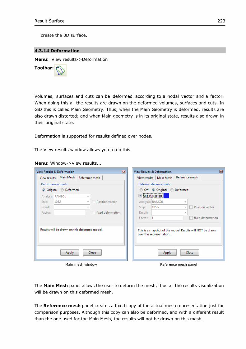
223Result Surface
create the 3D surface.
4.3.14 Deformation
Menu: View results->Deformation
Toolbar:
Volumes, surfaces and cuts can be deformed according to a nodal vector and a factor. When doing this all the results are drawn on the deformed volumes, surfaces and cuts. In GiD this is called Main Geometry. Thus, when the Main Geometry is deformed, results are also drawn distorted; and when Main geometry is in its original state, results also drawn in their original state.
Deformation is supported for results defined over nodes.
The View results window allows you to do this.
Menu: Window->View results...
Main mesh window Reference mesh panel
The Main Mesh panel allows the user to deform the mesh, thus all the results visualization will be drawn on this deformed mesh.
The Reference mesh panel creates a fixed copy of the actual mesh representation just for comparison purposes. Although this copy can also be deformed, and with a different result than the one used for the Main Mesh, the results will not be drawn on this mesh.

224 Reference Manual
In the upper part of this window, you choose between the Original state of the Main Geometry and the Deformed state, for which a nodal vectorial result, and an analysis and step, must be selected and a factor entered.
There is also a Reference Geometry option. This lets you visualize volumes, surfaces or cuts like Main Geometry does, but NO results can be displayed over these volumes, surfaces or cuts. It is merely provided as a reference, to contrast several deformations or changes in the original geometry. Remember that the current Mesh Display Style will be used for the Reference Geometry and it can only be changed when redoing the mesh.
In the lower part of the window, the Reference Geometry can be configured. You can choose between:
Off, so this reference visualization is not displayed;Original, if Main Geometry is deformed and you wish to compare it to its original state without losing a results representation;Deformation, where after providing an analysis, step, result and factor, you can use it to contrast two deformation states, or a deformed state and an original geometry; orColor, where the colour of the reference meshes can be specified as the same as, or different from, the original meshes.
There are two more interesting options:
Position vector: normally the deformation result is relative to the original coordinates of the mesh, but if the result is a new absolute position for the nodes of the mesh, then the user should check this option.fixed deformation: if this option is checked, the deformation will use the same fixed factor, instead of using the GiD suggested one, which varies acording to the magnitude of the deformation.
4.3.15 Line Diagram
Menu: View results->Line Diagram
This result visualization option is only active when line elements are used in the mesh, and will only be represented over these line elements. When using this result visualization option, graph-style lines will be drawn over the line elements.
When drawing a Scalar Diagram , the graph-style lines are drawn on a plane parallel to the screen (with its normal vector pointing out of the screen) when this result view is selected. The positive 'axis' will be the vector resulting from the cross product between this normal vector and the one that the line defines.
When drawing a Vector Diagram , the graph-style lines are drawn on a plane that

225Line Diagram
includes the result vector and the vector that the line defines. The graph-style lines represent the module of this vector. The positive 'axis' is also defined by the result vector. As modules are positive, to allow negative values, the input format for vector results allows the introduction of a fourth component: the signed vector module (see Postprocess results format: ProjectName.post.res from Customization Manual).
For ComplexVectors, their real part or their imaginary part can be selected to be drawn if the Vector Diagram visualization is used. If the modulus of the whole vector is selected, then both parts are drawn simultaneously.
There is a Show Elevations option only accessible through the Right buttons menu under Results -> LineDiagram -> Options. Elevations are lines that connect the nodes and the gauss points of the line element and the graph-style line that represents the result. The options are:
With the Show elevations option inside the menu Options -> Line Diagrams, you can choose how the elevations are drawn. Elevations are lines that connect the nodes and the gauss points of the line element and the graph-style line that represents the result. The options are:
None: to switch the elevations off; Nodes only: to draw the elevation lines only on the nodes; Whole line: to draw the elevation lines along the whole line, using nodes and gauss points; Filled line: to draw orange filled elevations; Contour filled line: the colors used to draw the filled elevations will be the same as a contour fill done along the line.
4.3.16 Line thickness
Menu: View results->Line Thickness
Toolbar:
With this visualization, the line elements will be drawn using the result's values as thickness.
This option uses a result component, or a scalar value, and draws the thickness of the lines according to this result. Lines are drawn as a four or eight sided prisms and the selected result is used as a radius of these prisms.
Line thickness is supported for results defined over nodes and over gauss points.
If the gauss points results can be globally smoothed, then a Smoothed sub-menu will be added with a list of the gaussian results, see View Results Menu -pag. 205-

226 Reference Manual
Line thickness using a result defined n lines with five gauss points, including the extrem points
Line thickness using the same result but globally smoothed
The colour of the thick lines can be adjusted with Options --> Result Surface --> Show elevations --> Contour fill, see Result Surface -pag. 222-.
4.3.17 Integrate
With this option the user is able to:
This step: get the integral value of a scalar or vectorial result over a set of elements.All step: get a graph of the integral values across all the analysis steps, of a scalar or vectorial result over a set of elements.
4.3.18 Distribution...
Menu: View results->Distribution
This option opens a window that shows information about the amount of entities with result on each span from a minimum and maximum of the result values.
Result must be an scalar or the modulus of a vectorial result or a component
The kind of graphs is similar to the 'Mesh quality' tool of preprocess.

227Distribution...
Result distribution window
There are two visualization modes:
Normal: The graph shows the amount of items on each span.Accumulated: The graph shows the number of items which have of a equal or smaller result value.
In the Result distribution window, if you double click on a value, the items below this value are selected in red.
4.4 Options Menu
4.4.1 Legends
Menu: Options->Legends
Legends appear when contour visualization, isosurfaces or color vector visualization is used:
Show: Legends can be switched On or Off.Opaque: Legends can be transparent, showing the result visualization behind them, or opaque.Show title: With this option the result name of the current visualization appears at the top of the legend.Draw user limits: If enabled, the maximum and minimum value of the legend will be surrounded with a box it these where fixed by the user.Border: If enabled, draws a box arround the legend and commentsChange title: Allows the user to change the title of the legend.Outside: Activating this option, the legend is shown in a separate window, thus leaving

228 Reference Manual
more space in GiD's windows.Automatic comments: If this option is activated, information about the type of analysis, the actual step and the kind of result, is added at the bottom of the screen (see Comments -pag. 105-).
4.4.2 Reference axes
Menu: Options->Reference axes
Allows the user to draw a reference frame for the model, being able to:
display the x, y, z axis, and change their coloursdisplay a reference grid for each of the xy, yz, xz planesdefine the number of subdivisions for the grid referencechange the colours of all these.
The configuration options of the reference axes are:
an example of this option can be seen in this image:
229Geometry
4.4.3 Geometry
Menu: Options->Geometry
Through this menu geometry related options can be set.
4.4.3.1 Border angle
Menu: Options->Geometry->Border angle
Allows the user to define the angle criteria between faces to consider the shared edge a boundary edge, i.e. sharp edge, or not. Angles between normals of adjacent faces smaller than the criteria set will be considered a shard edge and visualized when the meh style 'boundaries' is selected.
4.4.3.2 Massive body
Menu: Options->Geometry->Massive body
All interior elements are drawn. For tetraedra and other volume elements, the interior triangles and quadrilaterals are also drawn. This will increase enormously the amount of elements to be drawn, i.e. the visualization will become VERY SLOW.
4.4.3.3 Transparent
Menu: Options->Geometry->Transparent
All the meshes are drawn transparent by selecting this option.
4.4.3.4 Opaque
Menu: Options->Geometry->Opaque
All the meshes are drawn opaque by selecting this option.
4.4.3.5 Point options
As points can be viewed, there are several interesting options for each of them.
Menu: Options->Geometry->Point options...
Point options:

230 Reference Manual
Point options window
Here you can select whether to draw the points Quick, Internal texture, Nicely or with the center of a Texture glued to the point.
Quick: spheres and circles will be drawn as big dots. Internal texture: an image is used to drawn spheres and circles; it's a compromise between quality and speed.Nice: a triangle mesh, between 4 and 630 triangles big, is used to drawn each sphere and circles for a nicer quality.Texture: selveral images can be selected and will be used to draw on the point elements, using the point coordinates as the centre of the images. For a certain point, at each redraw the next image of the collection will be used.Point size factor: factor to be applied to the spheres and circles radii to increase the simze of the drawn elements.Result's size: a result can be selected and will be used as radius of the drawn points.Nice detail: level of detail used to draw the spheres and circles in Nice mode. Higher detail level will draw more triangles for each sphere or circle.
Note: The changes affect the representation of all the points - point elements and the arrow heads of vectors when using the Point detail level (see Display Vectors -pag. 213-).
4.4.3.6 Sphere options
As sphere and circle elements can be viewed, there are several interesting options for each of them.
Menu: Options->Geometry->Sphere options...

231Sphere options
Point options:
Here you can select whether to draw the spheres and circles Quick, with an Internal texture or Nicely.
Quick: spheres and circles will be drawn as big dots. Internal texture: an image is used to drawn spheres and circles; it's a compromise between quality and speed.Nice: a triangle mesh, between 4 and 630 triangles big, is used to drawn each sphere and circles for a nicer quality.Sphere size factor: factor to be applied to the spheres and circles radii to increase the simze of the drawn elements.Nice detail: level of detail used to draw the spheres and circles in Nice mode. Higher detail level will draw more triangles for each sphere or circle.
4.4.3.7 Line options
Menu: Options->Geometry->Line options...
As lines can be viewed, there are several interesting options for each of them.

232 Reference Manual
Line options window
Here you can select whether to draw the lines with a Quick style or a Nice one. Selecting a Line Size of 0.0 in the Nice style, will cause the lines not to be drawn. Quick: lines are drawn as 3-point thick lines. The line size is fixed. Nice: lines are drawn as long 4-sided or 8-sided prisms. The size and width of the lines can be changed. When the lines are drawn nicely, the number of sides of the prism used to draw them can be changed between 4 and 8 sides.
Note: Line options no longer affect the stream lines as before, but only the line elements. For stream lines options see Stream Lines -pag. 217-.
4.4.3.8 Change edge colour
Menu: Options->Geometry->Change edge colour...
With this option, the user is able to define the colour to be used to draw edges, instead of the default black colour.
4.4.3.9 Covering mesh
Menu: Options->Geometry->Covering mesh
Another feature in GiD is the calculation of the involving mesh of a set of points or nodes. To switch the visualization of this mesh on and off just select Options -> Geometry -> Covering mesh. After saying 'Yes' to the visualization of the covering mesh, you will be asked for a number. This number is the distance between the covering mesh and the points.
This option is not only available for points, but also for every mesh/set present in GiD.

233Covering mesh
Note: This covering mesh is recalculated when the mesh is deformed. So in a particle movement system the covering mesh will also move along with the particles.
This mesh can also be saved through Files -> Export -> Cover mesh.
4.4.3.10 Create delaunay meshes
Menu: Options->Geometry->Create delaunay meshes
This option allows the user to create delaunay meshes from the nodes of the postprocess model in three ways:
One for each visible mesh: creates separate delaunay meshes, one for each displayed mesh/set/cut Single mesh for all visible meshes: creates a single delaunay mesh from the nodes of the displayed meshes/sets Single mesh for all points: creates a single delaunay mesh from all the loaded points in postproces, belonging or not to an existing mesh/set.
After the delaunay mesh(es) creation GiD applies an alpha shape algorithm to delete detect contours the the mesh, if possible.
4.4.3.11 Extract boundaries
Menu: Options->Geometry->Extract boundaries
Extracts boundaries from shown volume and surface meshes; for each mesh creates a new set with its boundary elements. The original mesh is left untouched.
4.4.3.12 Separate connected components
Menu: Options->Geometry->Separate connected components
Separates connected components from shown volume and surface meshes.
For each mesh detects groups of connected elements and stores them in separate sets.
For instance a single volume mesh which corresponds to three unconnected spheres will be separated into three sets each one containing the volume elements of a single sphere. The original mesh is left untouched. By default a maximum of 50 connected groups will be separated into separated sets. This limit can be modified with the variable Utilities --> Variables --> PostMaxNumComponents on the main's window the right menu.
4.4.3.13 Swap orientation of visible surface meshes
With this options the orientation of the visualized surface elements, triangles and quadrilaterals, are changed so that the normal orientation is changed too. This option is useful in combination with the culling ( of front and back faces) visualization option, see View style -pag. 234- and Toolbars -pag. 12-.

234 Reference Manual
4.4.4 Change color
Menu: Options->Change Color
Allows the user to change the colour of each single mesh.
4.4.5 Change name
Menu: Options->Change Name
Allows the user to change the mane of each single mesh.
4.4.6 Other options
The options related with results are explained together with result explanation.
You can find the explanation inside each result on View Results Menu -pag. 205-
Under the Utilities menu there are other interesting options for postprocessing, take a look specially the ones that are (only Postprocessing) Utilities Menu -pag. 77-
4.5 Window Menu
Menu: Window
From this menu you can open the main windows.
4.5.1 View style
Menu: Window->View style...
Toolbar:
Below in an example of the View Style window, where almost all the interesting visualization options can be adjusted. It only deals with meshes, sets or cuts, and not with results.

235View style
View Style window
Selecting Volumes, Surfaces and/or Cuts, you can switch them On and Off, Delete them or rename them. By clicking on a Volume, Surface or Cut, and pressing Color... you can adjust the appearance of the selected set; you can change the color, including the Ambient, Diffuse, Specular, Shininess and transparency components, and return it to its Default color. The Diffuse component is used for all the representations, while the others (Ambient, Specular and Shininess) have more effect in Render visualizations.
Also separate styles can be selected for each mesh independently, just by clicking on the icon in the column eith the header 'St '.
Other interesting options which can be set for each individual mesh are:
I/O: Switch the mesh on and off
Toolbar: Switch on/off Volumes, Surfaces and Cut sets respectively
Tr: Enable or disable the transparent mode for the mesh Int: Draw or not the interior elements of the mesh Ew: Sets the edge width of the mesh.
In the Style menu you can choose how volumes, surfaces and cuts should be drawn. These options are:
Boundaries: All the edges of the boundaries and surface elements will be displayed in black. An edge is the line that belongs to just one surface element, or that belongs to two surface elements as long as the faces form an angle smaller than has been
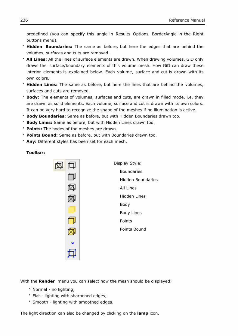
236 Reference Manual
predefined (you can specify this angle in Results Options BorderAngle in the Right buttons menu). Hidden Boundaries: The same as before, but here the edges that are behind the volumes, surfaces and cuts are removed. All Lines: All the lines of surface elements are drawn. When drawing volumes, GiD only draws the surface/boundary elements of this volume mesh. How GiD can draw these interior elements is explained below. Each volume, surface and cut is drawn with its own colors. Hidden Lines: The same as before, but here the lines that are behind the volumes, surfaces and cuts are removed. Body: The elements of volumes, surfaces and cuts, are drawn in filled mode, i.e. they are drawn as solid elements. Each volume, surface and cut is drawn with its own colors. It can be very hard to recognize the shape of the meshes if no illumination is active. Body Boundaries: Same as before, but with Hidden Boundaries drawn too. Body Lines: Same as before, but with Hidden Lines drawn too. Points: The nodes of the meshes are drawn. Points Bound: Same as before, but with Boundaries drawn too.Any: Different styles has been set for each mesh.
Toolbar:
Display Style:
Boundaries
Hidden Boundaries
All Lines
Hidden Lines
Body
Body Lines
Points
Points Bound
With the Render menu you can select how the mesh should be displayed:
Normal - no lighting;Flat - lighting with sharpened edges;Smooth - lighting with smoothed edges.
The light direction can also be changed by clicking on the lamp icon.

237View style
Toolbar:
Change light direction
Near the Culling label, you can choose whether the Front Faces or Back Faces are culled, i.e. not drawn, or No Faces are culled. This option is useful for looking at volume meshes, etc.
Toolbar:
Culling Style:
No Faces
Front Faces
Back Faces
Both geometry and mesh conditions can also be drawn if they are present in preprocess.
The following two options can be changed separately for each mesh/set/cut:
Massive lets you see the elements that are inside a volume mesh, and draw all the vectors inside a volume/surface/cut when a Boundaries display style is used.
Transparent determines whether the volumes/surfaces/cuts will be drawn as transparent or opaque, so that, for instance, isosurfaces inside them can be viewed easily.
4.5.2 View results
Menu: Window->View results...
Toolbar:

238 Reference Manual
View results window
The View Results window manages the visualization of the following type of results:
Contour fillSmooth contour fill ( of gaussian results globally smoothed), same as the menu Contour fill --> SmoothedContour ranges (if Result Range Tables are present)Contour linesSmooth contour lines ( of gaussian results globally smoothed), same as the menu Contour lines --> SmoothedDisplay vectorsShow min/maxResult surfaceSmooth result surface ( of gaussian results globally smoothed), same as the menu Result surface --> SmoothedLine thicknessSmooth line thickness ( of gaussian results globally smoothed), same as the menu Line thickness --> SmoothedScalar and Vector line diagram (if line elements are present)
For each individual visualization options, please look at the corresponding chapter.
For the 'Main mesh' and 'reference mesh' panel, please look here: Deformation -pag. 223-.
To get the results grouped in folders like the image, please look at the format of the results specified on Customization Manual
4.5.3 Animate
Menu: Windows->Animate...

239Animate
Toolbar:
With this window a little bit of automatization has been done to create animations inside GiD. Nowadays, almost all results visualizations are animated. Only stream-lines are not automatized along all the steps of the current analysis.
Animate window
Some animations can be done with combined results visualization, from the same or different analisis, for instance an isosurface animation from OLS result of ODDLS analysis with a contour fill of Pressure of the RANSOL analysis can also be done with this window. The only constraint is that the number of steps and the step values should be the same in both analysis.
This window lets you create an animation of the current Results View, where the limits can be fixed along the animation with Automatic Limits, and/or an animation of the Deformation of the meshes. Step number and step value are shown. On the slide bar, the step number is shown.
The four buttons under the slide bar are self-explanatory: they 'Rewind', 'Stop', 'Play' and 'Step' the animation. Clicking on the slide bar will rewind or advance the animation. The green LED, which indicates that an animation is ready, will change to red while the animation is being saved to a file. This LED will change back to green when the animation is finished, or the 'Stop' button is pressed.
Options are:
Automatic Limits: GiD searches for the minimum and maximum values of the results

240 Reference Manual
along all the steps of the analysis and uses them to draw the results view through all the steps. Previously, it needs to visualize some resutls. Deformation: Permits to record animation with a specific deformation. Endless: The animation continues indefinately. Total time: Specfies the duration of the clip. Delay: Specify a delay time between steps in milliseconds. Use step values as seconds: The number of step will be used to the duration of the clip. From step I to step K: Allows the user to do an animation between step number I and setp number J , both included. This is also useful to skip the first step of an animation of a deformed mesh with a result visualization, which is the original state of the mesh, without deformation and without the result visualization. Save TIFF/JPEG/GIFs on: Save snapshots, in TIFF, JPEG or GIF format, of each step when the 'Play' button is pushed. Here the filename given will be used as a prefix to create the TIFF/JPEG/GIFs; for instance, if you write MyAnimation, TIFF/JPEG/GIF files will be created with names MyAnimation-01.tif/MyAnimation-01.gif, MyAnimation-02.tif/MyAnimation-02.gif, and so on. Save animation: by checking this options and entering a filename a movie clip will be saved ( by pressing play) with the selected compression method. The supported formats are:
MPEG: uses the MPEG-2 standard algorithm to encode the frames, creating an .mpg video.AVI mjpeg: using jpeg compression for each frame.AVI MS Video 1: using Microsoft(R)'s Video 1 compression algorithm.AVI raw True Color: no compression, in 24 bpp ( 16 million colours).AVI raw 15 bpp (VD): no compression but in 15 bpp ( 32 thousand colours).AVI raw 16 bpp (MS): no compression but in 16 bpp ( 65 thousand colours).GIF no dithering: creates an animated gif image, reducing the number of colours to 256 ( creating some band artifacts).GIF dithering595: creates an animated gid image, reducing the number of colours to 256 but applying a dithering algorithm to reduce the band artifacts. The rgb palette used in the dithering algorithm is based on 5 reds, 9 greens and 5 blues.GIF dithering666: creates an animated gid image, reducing the number of colours to 256 but applying a dithering algorithm to reduce the band artifacts. The rgb palette used in the dithering algorithm is based on 6 reds, 6 greens and 6 blues.Macromedia Flash Video ( .flv): creates Macromedia (R) flash video using the Screen video compression format.
Note: To avoid problems when trying to view an MPEG format animation in Microsoft Windows , it is strongly recommended that you use the Default menu to select a 'standard' size and press the Resize button. The graphical window will change to this 'standard' size. After finishing the animation, simply select Default on the menu and press the Resize button, and the previous size will be restored.
Note: AVI MS Video 1 uses a simple video compression algorithm, commonly supported by all video players. It is the recommended when the movie is to be included in

241Animate
presentations. To reduce the size of the animation file, the user can set the Utilities --> Variable -->AviMSVCUsePreviousInfo option, on the right buttons menu ( see User Interface -pag. 9-),to 0 or 1, and verify the created animations with their platform configuration.
Note: Macromedia Flas video is suitable for web sites.
Note: If you want to recompress the animation with another codec, like xvid, the AVI raw True Color is recommended, as it saves each frame without compression.
Create a stereoscopic animation: Permits to create a stereoscopic animation which for each frame the left eye view and the right view are saved, i.e. efectively doubling the width of the frames. Special software video players, and hardware, are needed to view this animation correctly. Only AVI format is supported at the time. Static analysis animation profile: If the project has only one step, it is possible to simulate an animation by generating intermediate steps. Use this option to automatically generate several frames, following a lineal, cosine, triangular or sinusoidal interpolation between the normal state and the deformed state. Default: This comobobox permits to choose the resolution of the clip.
Profile factor for pseudo-animation
4.5.4 View graphs
Menu: Window->View graphs...
Toolbar:
All the operations related with graphs can be done through this window.
The window is divided in a top bar and three tabs. The top bar allows users to change between the created graph sets, create a new one, delete or rename an existing one.

242 Reference Manual
The tabs are:
Plot graph: The graphs of the current graph set are drawn in this tab. the current graph set is the one selected in the top bar. A quick way to access to the options of a particular graph is to double click in any point of the desired graph. Contextual menu also offers manegement options in this layout. For example user can view labels for the points of a graph. These labels include not only the graph point's number, but also its X and Y values. The labels that have been selected on this tab also appear in the results view.
Create: This tab is used to create the graphs in the current graph set. User can choose between these options:
No graph: deletes all the graphs in the current graphset.Point evolution: a graph of the evolution of the selected result along all the steps, of the default analysis, is created after pressing the 'Apply' button and selecting some nodes or points. Point graph: a graph of one result against another of the selected results is created after pressing the 'Apply' button and selecting some nodes or points. The option 'all steps' shows the cross-result evolution along all steps inside the default analysis.Border graph: displays a graph of the results on the selected border, using the x, y, z or line distance as abscissa.Line graph: also called 'section graph' displays a graph defined by the line conectig two selected nodes of surfaces or volumes, or any arbitrary points on any projectable surface and in any position.Integrate scalar: graph of an integrated result over a mesh.Integrate vector normal: graph of an integrated result over a mesh.Integrate vector tangential: graph of an integrated result over a mesh.Point complex evolution: similar to 'Point Evolution' but for complex results, where both real and imaginary part of the result are displayed as 'x' and 'y' in the

243View graphs
graph.
Options: This tab is used to change several options related with graph sets and graphs. All the sets and graphs are organized in tree shape in order to get a quick view. Selecting each item in the tree the options changes. There are two diferent layouts depending if a graph set or a graph is selected.
Graph set options: Several settings related with the current graph set can be changed.
Graph options: User can set several options related with the style as the color, the

244 Reference Manual
line width, etc. Graphs can also be deleted or renamed.
4.5.5 Several results
Menu: Window->Several results...
With this window user can select whether to view the results one by one, as usual, or to view some results visualization types at once, e.g. a contour fill of pressure and velocity vectors at the same time. From this window you can also delete the undesired results visualizations. After selecting the desired behaviour, press the Apply button.
Several Result window

245Several results
Example showing contour fill, vectors and the minimum and maximum visualization types
4.5.6 Results ranges table
Menu: Window->Results ranges table...
Creates ranges, with names, for the results, so that they can be displayed with the contour ranges options, which draws a c.fill with the defined ranges and displays the text in the legend.
Results ranges table window
Example:
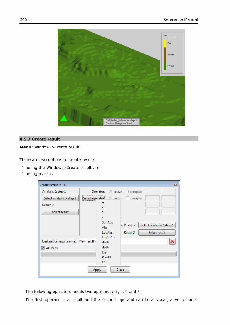
246 Reference Manual
4.5.7 Create result
Menu: Window->Create result...
There are two options to create results:
using the Window->Create result... or using macros
The following operators needs two operands: +, -, * and /.
The first operand is a result and the second operand can be a scalar, a vector or a

247Create result
result. These operations are done component-wise, and so, both results should be of the same type.
If result1 = ( r11, r12, ..., r1n) then if second operand is
a scalar then the result is ( r11 op scalar, r12 op scalar, ..., r1n op scalar);
a vector then the result is ( r11 op v1, r12 op v2, r13 op v3[, r14 op v4]) ( so result1
should be a vector); a result ( result2) then the result is ( ( r11 op r21, r12 op r22, ..., r1n op r2n).
The other operators needs a result as operand.
If result2 = ( r21, r22, ..., r2n) is the operand then:
Abs: The result is ( abs( r21), abs( r22), ..., abs( r2n));
SqrtAbs: The result is ( sqrt( abs( r21)), sqrt( abs( r22)), ..., sqrt( abs( r2n)));
LogAbs: The result is ( log( abs( r21)), log( abs( r22)), ..., log( abs( r2n)));
Log10Abs: The result is ( log10( abs( r21)), log10( abs( r22)), ..., log10( abs( r2n)));
db10: The result is ( 10·log10( abs( r21)), 10·log10( abs( r22)), ..., 10·log10( abs(
r2n)));
db20: The result is ( 20·log10( abs( r21)), 20·log10( abs( r22)), ..., 20·log10( abs(
r2n)));
Exp: The result is ( er21, er22, ..., er2n);Pow10: The result is ( 10r21, 10r22, ..., 10r2n);1/: The result is ( 1 / r21, 1 / r22, ..., 1 / r2n).
Toolbar:
Nodal scalar to vector window

248 Reference Manual
In the figure above it can be seen highlighted the icon of the macro 'Convert a scalar to a vector'.
With this macro the user can create a vector from a scalar result using the entered vector, by multiplying the vector with the scalar value. This operation can be applied to all the steps of the analysis with the 'all steps' option.
Toolbar:
In the figure above it can be seen highlighted the icon of the macro 'Create statistical scalar result'.
With this macro the user can create a scalar result where each value-i is the maximum, minimum or average of all values-i of the selected result on all steps.
4.5.8 Create statistical result
Menu: Window->Create statistical result...
This window allows the user to create a statistical result from previous results.
User can choose between several operators:
minimum maximum average accumulated standard deviation integral value ( with an option to add an initial value for step 0.0, if it is not present in the analysis)

249Create statistical result
The new result will be created at the last step of the analysis, in which each nodal value will be the minimum, maximum, average, accumulated, standard deviation or integral, of all the values at that node for all the selected steps of the analysis. When integral value operator is selected some options can be set just clicking the options button.
The name of this new result can also be defined in this window.
4.5.9 Create graphs
Menu: Window->Create graphs...
With this window the user can create graphs from other graphs.
The following operators needs two operands: +, -, * and /.
The first operand is a result and the second operand can be a literal or a graph. These

250 Reference Manual
operations are done on the selected components and the graphs needs to have the same number of values.
The 'fit' operator needs two graphs.
If graph1 = ( g1x1, g1x2, ..., g1xn) and ( g1y1, g1y2, ..., g1yn) then if second operand is
a literal then the resultant graph is ( g1x1 op literal.a, g1x2 op literal.a, ..., g1xn op
literal.a) and ( g1y1 op literal.b, g1y2 op literal.b, ..., g1yn op literal.b)
a graph ( graph2) then the result is ( ( r11 op r21, r12 op r22, ..., r1n op r2n).
The other operators needs a graph as operand and the axis to be precessed can be selected in some of them.
If graph2 = ( g2x1, g2x2, ..., g2xn) and ( g2y1, g2y2, ..., g2yn) is the operand then:
Abs: The result is ( abs( g2x1), abs( g2x2), ..., abs( g2xn)) or ( abs( g2y1), abs(
g2y2
), ..., abs( g2yn));
SqrtAbs: The result is ( sqrt( abs( g2x1)), sqrt( abs( g2x2)), ..., sqrt( abs( g2xn))) or
( sqrt( abs( g2y1)), sqrt( abs( g2y2)), ..., sqrt( abs( g2yn)));
LogAbs: The result is ( log( abs( g2x1)), log( abs( g2x2)), ..., log( abs( g2xn))) or (
log( abs( g2y1)), log( abs( g2y2)), ..., log( abs( g2yn)));
Log10Abs: The result is ( log10( abs( g2x1)), log10( abs( g2x2)), ..., log10( abs(
g2xn
))) or ( log10( abs( g2y1)), log10( abs( g2y2)), ..., log10( abs( g2yn)));
db10: The result is ( 10·log10( abs( g2x1)), 10·log10( abs( g2x2)), ..., 10·log10( abs(
g2xn))) or ( 10·log10( abs( g2y1)), 10·log10( abs( g2y2)), ..., 10·log10( abs( g2yn)));
db20: The result is ( 20·log10( abs( g2x1)), 20·log10( abs( g2x2)), ..., 20·log10( abs(
g2xn))) or ( 20·log10( abs( g2y1)), 20·log10( abs( g2y2)), ..., 20·log10( abs( g2yn)));
Exp: The result is ( eg2x1, eg2x2, ..., eg2xn) or ( eg2y1, eg2y2, ..., eg2yn);Pow10: The result is ( 10g2x1, 10g2x2, ..., 10g2xn) or ( 10g2y1, 10g2y2, ..., 10g2yn);1/: The result is ( 1 / g2x1, 1 / g2x2, ..., 1 / g2xn) or ( 1 / g2y1, 1 / g2y2, ..., 1 /
g2yn);
derivate: Will create a graph with the derivate values of graph2: ( g2x1 + offset * (
g2x2 - g2x1), g2x2 + offset * ( g2x3 - g2x2), ..., g2xn-1 + offset * ( g2xn - g2xn)) and
( ( g2y2 - g2y1) / ( g2x2 - g2x1), ( g2y3 - g2y2) / ( g2x3 - g2x2), ..., ( g2yn - g2yn-1) /
( g2xn - g2xn-1)), offset can be set by the user;
integral: Will create a graph with the accumulated values of graph2: ( g2x1, g2x2,
g2x3, ..., g2xn) and ( 0, SumArea( g2x1 ... g2x2, g2y1 ... g2y2), SumArea( g2x1 ...
g2x3, g2y1 ... g2y3), ..., SumArea( g2x1 ... g2xn, g2y1 ... g2yn);
fit: Will fit the bounding box of graph2 to the bounding box graph1, also the x or the y axis can be fitted;dFT: Does the discrete fourier transform on graph2, fat fourier transform if the number of values is power of 2, several options can be set by the user with the following options window ( the create polar graph calculates the modulus for the x values and the phase for the y values which can be used to draw the polar graph

251Create graphs
using the Window --> View graphs window):
inv-dFT: Calculates the inverse discrete fourier transform using the x-values and y-values as the real and imaginary part of the complex;CubicSpline: Interpolates a graph using cubic splines and the user can define the number of steps between the graph values;CatmullRomSpline: Interpolates a graph using Catmull-Rom splines and the user can define de number of points along the interpolated graph; the picture below shows the difference between these two spline types when interpolating a simple 4 point graph, in red:
4.6 Results' cache

252 Reference Manual
How it works
Result cache block diagram
The Result's cache mechanism allows the analysis and visualization of lots of results which, otherwise, could not be held entirely in memory.
Instead of loading all results from the file(s), a certain amount of memory, a memory pool, is reserved and used to load and unload the result values as they are needed.
When this mechanism is enabled and a result's file is loaded, GiD verifies the correctness of the file and gets some information about the results, such as minimum and maximum values, amount of memory needed, position in file.
If a result is selected to do, for instance, a contour fill visualization and it's not in memory, then GiD checks if there is enough space in the memory pool and loads it. If it's already in memory, the time-stamp of the result is actualized.
If there is not enough space in the memory pool to load the desired result, then the oldest results are unloaded and their memory freed until there is enough memory to load the desired result.
What's cached: Only results which are already stored in files are cached, i.e. files read with Files --> Open, Open multiple or Merge.
What's not cached: When cuts, extrusions are done or isosurfaces are converted to full featured meshes the generated results are held in memory. Results created in GiD using the Window --> Create result, Create statistical result are held in memory. Also results imported using Files --> Import or using the plug-in mechanism or the TCL procedure GiD_Result create ... are held in memory too.
In order to cache these results, save the model, with Files --> export --> Post information --> whole model and open it again.
Options
The user can enable the Result's cache in the postprocess panel of the Utilities --> Preferences window. The size of the memory pool can also be adjusted by selecting one of the predefined memory sizes or entering the desired amount in the same entry. The size can be

253Results' cache
adjusted according to not only the amount of memory the computer has, but also the memory used by a single result. Using indexed binaries, will speed up the access of the results on huge file, more over if the user access them randomly.Using indexed results information stored in the indices, will speed up the loading of huge results files, as the results information, except values, are already stored in the index files.
Note: if for some reasons GiD has problems reading the index files, or the information stored in these files are not actualized, the user can recreate these index file in the File --> Open dialog box, see Open -pag. 30-.
Results' cache options
For instance a mesh with one million nodes with a vector result at each step, the amount of memory needed to hold the nodal vector result of a single step will be: 4 components * 4 bytes per float * 1 million nodes = 16 MBytes of memory. If there are 100 steps in the analysis and an animation of these vectors is desired, to get a fluid animation the memory pool must be set to 16 * 100 = 1.6 GBytes of memory. But if the desired animation is of a contour fill or an iso-surface, then the amount of memory needed is reduced by 4, to 400 MBytes.
Caution
When the result's cache is used, the result's files remains opened, to make the retrieval of the results faster.
If a simulation is done on a cluster where the model is partitioned in 1024 pieces then 1024 separated result's files are generated.
When these 1024 result's files are merged in GiD with the result's cache mechanism

254 Reference Manual
enabled, then the 1024 files will still be opened!
Usually in Linux the maximum number of opened files are, precisely, 1024, and some of them are already used, causing GiD to display an error when the user tries to merge these 1024 result's files.
This limit on the number of open file descriptors is one of the limits imposed by the system, like the cputime, coredumpsize, datasize, etc. There are two types of limits in Linux, soft limits and hard limits. Usually the soft limits can be changed by the user, but administration privileges are needed to change the hard limits.
Sometimes soft and hard limit are not the same, and the user is able to raise the number of open file descriptors to its hard limit. If the user uses the bash shell, then the commands ulimit -Sn ( open files soft limit) or the ulimit -Hn ( open files hard limit) should be checked. An additional parameter can be entered to modify the limit, for instance ulimit -Sn 2048. In csh/tcsh the command is limit [ -h] openfiles
Note:
if we convert a cut mesh, see Do Cuts Menu -pag. 202-, to a full featured mesh, then the results for this cut are created and are not cached. If this information is saved using the Files --> Export --> Post information --> whole model' and read again, then the results on the cut mesh will cached as the other results too, and GiD will again use a modest amount of memory.

255Results' cache

256 Reference Manual

INDEX
257
3
3d view 66
3DStudio mesh 39
A
About 132
ACIS read 36
ACIS write 51
Actualize problem type 158
analysis selection 205
angle 124
Angle rotation 61
animate controls 106
Animation 238
Animation Window 238
Arc center 26
Arc creation 138
Arcs (swap) 150
Arrows operations 16
ASCII write project 51
ascii xyz import 47
Assign condition 161
Assign material 164
automatic comments 105
automatic comments patterns 105
Automatic NURBS surface 138
Automatic rotation center 60
AVI files 238
B
Background colours 82
Background Image 74
background mesh 168
Base option in points 24
Basics 3
Batch file 45
batch window 104
beam diagrams 224
body 234
body with boundaries 234
body with lines 234
Boolean surface operations 156
Boolean volume operations 156
Boundaries 234
By chordal error 168
By geometry 168
C
Calculate 198
Calculate remote 198
Calculate window 198
Calculation file 52
Calculator 111
Calling GiD 5
Cancel process 198
Center (rotation) 60
CGNS mesh 39
changing cut color 234
changing mesh color 234
changing set color 234
Chordal error 168
Circle 144
Circle options 230
Clip planes 65
cloud points meshing 47
Collapse 193
color selection 234
Colours of entities 82
Command line 16

258 Reference Manual
Command line arguments 5
comment format 105
Comments 105
comments parameters 105
Comments patterns 105
Complex numbers 224
Complex vectors 217
Conditions 160
cone 144
Configuration file 102
Contact copy 113
Contact surface creation 141
Contact volume creation 143
contour fill 209
contour lines 212
Contour lines width 212
contour method 42
contour ranges 212
convert cuts to sets 202
convert to cuts 215
Convert to NURBS line/surface 153
Coon's surface 145
Coordinates 22
Coordinates window 103
Copy 113
Correct sizes 168
cover mesh 232
Create 4-sided surface 145
Create 4-sided surface automatically 146
Create arc 138
Create contact surface 141
Create contact volume 143
Create entities 133
Create line 133
Create line (straight) 133
Create NURBS line 134
Create NURBS surface 138
Create planar surface 146
Create point 133
Create polyline 137
Create volume 142
CreateBoundaries 194
Customizing Problem type registration 131
Cut planes 202
Cuts 202
cylinder 144
Cylindrical coordinates 23
D
Data 157
data report 51
Debugger 160
deform mesh 223
delaunay mesh of point clouds 47
Delete entities 147
Delete nodes/elements 193
display style 234
display vectors 213
Distance 124
distance 124
Divide 147
Divide meshes 202
Draw 187
Draw again 62
Draw assigned sizes 187
Draw condition 163
Draw Element Type 189
Draw material 165
Draw Mesh / No mesh 189
Draw RjumpSkip 189
Draw Sizes 187

259INDEX
Draw Structured Type 189
Drawing method 83
DXF read 35
DXF write 50
Dynamic box 26
Dynamic pan 62
E
Edit entities 147
Edit mesh 191
Edit NURBS line/surface 151
Element type 181
Elements (structured) 176
End session 58
Entering cylindrical coordinates 23
Entering global coordinates 23
Entering local coordinates 23
Entering points 20
Entering points by coordinates 22
Entering spherical coordinates 24
Entities informations 121
Entities labels 70
Entities selection 26
Entities share 113
Entities visualization 76
Erase elements 193
Erase entities 147
Erase mesh 191
Escape 28
Exchange material 165
Export 50
Export ACIS 51
Export ASCII project 51
Export calculation file 52
export data report 51
Export DXF 50
export GiD mesh 51
Export IGES 50
Extents (zoom) 58
Extrude 113
F
Fast draw mode 96
Fast rotation 83
Fast rotation in post-process 96
Fast visualization mode 83
Files 29
Filter 26
filter window 109
Filtering coordinates 96
Find entities 123
Force mesh 186
Force no mesh 186
Four-sided surface automatic creation 146
Four-sided surface creation 145
Frame 58
G
Gauss points in contour fill 209
Gauss points in smooth contour fill 205
Gauss points smooth option 209
General data 166
Generate mesh 190
Geometry 133
Geometry view 133
GiD basics 3
GiD themes 81
GIF sequence 238
Graph Lines 220
Graphical displacement 62
Graphs 220
Grid 26
H

260 Reference Manual
Hardcopy 56
Help 127
hidden boundaries 234
Hidden lines 234
Hide drawing regions 65
Hole NURBS surface 154
Hole volume 142
I
Icons 9
Id 123
Identity 123
IGES read 33
IGES write 50
Illumination 62
Image to clipboard 74
Import 32
Import 3DStudio mesh 39
import ACIS 36
Import CGNS mesh 39
import DXF 35
Import GiD mesh 39
import IGES 33
import NASTRAN 37
import Parasolid 35
import Rhino 36
import Shapefile 36
Import STL mesh 38
import VDA 36
Import VRML mesh 38
Indexed results file 30
Indexed results files 251
Info entities 121
Info problem 121
Initial view (rotation) 61
Insert geometry 46
Insert GiD model 46
Internal texture 230
Internet Retrieve 158
Intersection 155
intersection volume volume 156
Interval data 165
Intervals 166
Invoking GiD 5
Iso line 215
Iso Surface 215
iso surfaces colours 215
iso surfaces with results 215
Isoline 215
Isosurface 215
K
Keyboard shortcut 108
L
Label 70
Label format 96
Label lists (holes) 122
Layers 98
Layers ON save 52
Leaving commands 28
Legend format 96
legends 227
Line (straight) creation 133
line diagrams 224
Lines 234
Lines normals 71
Lines operations 149
Lines sense swap 71
List 121
Load 159
Local axes 167
Local/global coordinates 23

261INDEX
M
Macros 108
marching cube 42
Materials 163
Mcopy 113
Merging partitions 31
Merging postprocess files 31
Mesh cancel 191
Mesh criteria 186
Mesh edit 191
Mesh generation 190
Mesh quality 194
Mesh read 39
Mesh write 51
Meshing data reset 187
Mirror 113
Mode 75
Mouse 18
Move 120
Move node 191
Move point 147
Move screen objects 103
MPEG files 238
Multiple views 75
Multiple windows 75
N
NASTRAN read 37
New 29
Normal in surface option 25
Normal projection 65
Normals 71
Notes 113
NURBS line conversion 153
NURBS line creation 134
NURBS line edition 151
NURBS surface creation 138
NURBS surface hole 154
O
Object axes rotation 60
Offset 113
Online Help 127
Open multiple postprocess files 31
Open postprocess file 30
Open project 30
Open refinement files 31
OpenGL options 83
Option Arc center 26
Option base in points 24
Option normal in surface 25
Option point in line 25
Option point in surface 25
Option tangent in line 25
P
Page/image setup 57
Pan (graphical) 62
Parallel lines. NURBS surface 138
Parametric line 135
Parametric surface 140
Parasolid read 35
particle tracing 217
Perspective 65
Perspective projection 65
Planar surface creation 146
Plane XY (Original) 61
Plane XZ 61
Plane YZ 61
Point (show) 123
Point creation 133
Point definition 20
Point enter window 103

262 Reference Manual
Point in line option 25
Point in surface option 25
point options 229
Points 20
Points rotation 61
polygon 144
Polygonal cut 202
Polyline 150
Polyline creation 137
Post-processing change light vector 234
Post-processing culling 234
Post-processing Fast-rotation 234
Post-processing opaque 234
Post-processing render 234
Post-processing select meshes/sets/cuts 234
Post-processing transparent 234
Postprocess border angle 229
Postprocess introduction 199
Postprocess List file 30
Postprocessing no results 205
Postprocessing results 205
Preprocess/Postprocess 56
Print 58
Print to file 56
prism 144
Problem data 166
Problem information 121
Problem type 157
Problemtype 159
Q
Quadratic elements drawing 81
Quality of the mesh 194
Quit 58
R
radius 124
Read 3DStudio mesh 39
Read ACIS 36
Read batch window 104
Read CGNS mesh 39
Read DXF 35
Read IGES 33
Read NASTRAN 37
Read Parasolid 35
Read postprocess 30
Read project 30
Read Rhino 36
Read saved project 29
Read Shapefile 36
Read STL mesh 38
Read VDA 36
Read View 72
Read VRML mesh 38
Reading partitioned results 31
Recent files 31
Recreating index of results files 251
Redraw (graphical) 62
Register GiD 128
Register Problem type 130
Remove elements/nodes 193
Render 62
Renumber 122
Repair model 126
Report 112
Reset mesh data 187
Result as radius of points 229
Result surface 222
results over isosurfaces 215
results visualization 205
Results' cache 251
Rhino read 36

263INDEX
Right buttons menu 17
Rotate (graphical) 59
Rotate angle 61
Rotate center 60
Rotate object axes 60
Rotate points 61
Rotate screen axes 59
Rotate trackball 59
Rotation 113
S
Safe visualization mode 83
Save 29
Save as 32
Save ASCII project 51
Save ON layers 52
Save project 31
Save View 72
Save window configuration 102
scalar diagram 224
Scale 113
Screen axes rotation 59
Script file 45
Search entities 123
Search volume 142
select meshes/sets/cuts 234
Selecting points 26
selection filter 109
selection window 109
Semi-Structured 176
Sequence of commands 108
setting contour fill colors 209
several results 244
Shapefile read 36
Shortcut, keyboard 108
Show errors 193
show min max 213
ShowIsolines 215
Signal entities 123
simplified view 96
Simplify NURBS line/surface 154
Size of mesh 168
Smooth contour fill 209
smooth contour fill 205
Smooth elements 192
Smooth gauss points results 205
Smooth option for gaussian results 209
Smoothed results sub-menu 205
Solver 198
Spacing 168
sphere 144
Sphere options 230
Spherical coordinates 24
Spherical cuts 202
Split elements 191
Status 120
Stereoscopic animation 238
Stereoscopic movies 238
stereoscopic vision 66
STL mesh read 38
Straight line creation 133
stream line 2D constraint 217
stream lines 217
Structured 171
structured concentrate 175
Surface (4-sided) 145
Surface (planar) 146
Surface boolean operations 156
surface intersection 156
Surface mesh 142
Surface render precision 81
264 Reference Manual
SurfMesh 150
SurfMesh edition 150
Swap arc 150
Swap normals 124
Swap orientation 233
T
Tangent in line option 25
Tcl/Tk 160
text data report 51
Textures on points 229
Three-sided surface creation 145
TIFF sequence 238
Toolbars 101
Toolkit icons 9
Trackball rotation 59
Transform problem type 158
Translation 113
Trimmed NURBS surface 138
Type of element 181
U
Unassign condition 163
Unassign material 165
Uncollapse 155
Undo 77
Units 166
Unload 159
Unstructured 168
Up menus 28
Update problem type 158
User basics 20
User interface 9
Using this manual 1
Utilities 77
V
VDA read 36
vector colours 213
vector diagram 224
Vector filtering 213
vectors detail level 213
vectors options 213
View 58
View entities 76
View geometry 133
View higher entities 71
View process info 198
View Results window 205
Views, several 75
Visit GiD web 132
Visualization 58
visualization troubles 5
Volume boolean operations 156
Volume creation 142
volume intersection 156
VRML mesh 38
W
Window Configuration file 102
Windows 9
windows state 101
Word oriented 16
Write ACIS 51
Write calculation file 52
Write DXF 50
Write IGES 50
Write using template file 52
X
xyz import 47
Z
Zoom 58