maria leonilde r. varela* and antónio arrais-castro rita a ... · on the procurement management...

Int. J. Information and Decision Sciences, Vol. 10, No. 4, 2018 311

Copyright © 2018 Inderscience Enterprises Ltd.

A data fusion approach for business partners selection

Maria Leonilde R. Varela* and António Arrais-Castro Department of Production and Systems, School of Engineering, University of Minho, Azurém Campus, 4800-058 Guimarães, Portugal Email: [email protected] Email: [email protected] *Corresponding author

Rita A. Ribeiro UNINOVA – CA3, Campus FCT-UNL, 2829-516 Caparica, Portugal Email: [email protected]

Abstract: Strategies of market diversification push companies to provide novel products and services to customers, belonging to new geographic and demographic segments. Additionally, market development strategies targeting non-buying customers in selected segments or new buyers in new segments may be paired with increased product diversification and improved business agility. To fulfil the requirements associated with manufacturing, a wider range of products and increased customised demands imply having a wider set of competences available. Most companies find it increasingly difficult to have all required competences in their internal structures; therefore, they need to rely on strategic business partnerships and suppliers to be successful. In this paper, we discuss a data fusion decision approach for supplier and business partner evaluation, which includes past, current and forecast information about business partners. This approach may prove vital for companies to establish strong collaborative business networks.

Keywords: collaborative networks; supplier evaluation and selection; business strategies; dynamic multi-criteria model; data fusion; decision support methods and tools; fuzzy decision-making; uncertainty treatment.

Reference to this paper should be made as follows: Varela, M.L.R., Arrais-Castro, A. and Ribeiro, R.A. (2018) ‘A data fusion approach for business partners selection’, Int. J. Information and Decision Sciences, Vol. 10, No. 4, pp.311–344.

Biographical notes: Maria Leonilde R. Varela received her PhD in Industrial Engineering and Management from the University of Minho, Portugal in 2007. She is an Assistant Professor at the Department of Production and Systems of University of Minho. She has published more than 80 refereed scientific papers in international conferences and in international scientific books and journals.

312 M.L.R. Varela et al.

She coordinates R&D projects in the area of production and systems engineering, and she is a frequent paper reviewer for several journals. She is a member of several groups, namely of the Euro Working Group of Decision Support Systems and of the Machine Intelligence Research Labs.

António Arrais-Castro received his PhD in Production and Systems Engineering from the University of Minho in 2015. He is a technology addict and an enthusiastic manager. Previously, he was Glasses Group Global’s CTO, Jumia’s CTO @ Africa Internet Group | Rocket Internet, supervising the development of Africa’s largest eCommerce platform. Before that, he was CTO @ UNEDGED, supervising the development of innovative interactive software. He owns a PMP certification, issued by the Project Management Institute, and he is a Certified Prince2 Practitioner, by APMG International, a Certified Product Owner and a Certified Scrum Master, by the Scrum Alliance.

Rita A. Ribeiro obtained her BA in Management and Business Administration from the ISEG (PT) in 1981. She received her MSc in Information Systems Technology from the George Washington University, USA in 1988 and PhD in Artificial Intelligence from the University of Bristol, UK in 1993. Since 2002, she is the Head of the research group on Computational Intelligence at the UNINOVA. She is a Senior Researcher at the UNINOVA and an Invited Associate Professor at the New University of Lisbon. She has been involved in several national and international research projects, which include 16 financed ones. She has published more than 100 scientific papers.

This paper is a revised and expanded version of a paper entitled ‘Negotiation platform for collaborative networked organizations using a dynamic multi-criteria decision model’ presented at Group Decision and Negotiation 2014 (GDN 2014), Toulouse, France, 10–13 June 2014.

1 Introduction

Companies are facing growing challenges while trying to implement a globalised business strategy. Contemporary business models need to grow outside political and geographical boundaries. Developing products and implementing projects targeted at diverse cultural and political realities, significantly increase the range of operational and management skills.

Many works continue to arise focusing on the influence of stakeholders in the supply market evolution and its importance in supply chain business dynamics and management functions (Knight et al., 2015; Schenkel et al., 2015; Sjoerdsma and Van Weele, 2015).

Moreover, to implement strategies that require broader competences, companies must create a balanced mix between integrating in their internal structure operational, productive and engineering and management competences – required to autonomously implement the business model – and establishing closer relationships with business partners and suppliers to complement their own internal core competences. The increased competences will also have to support the business model, transparently from the point of view of the customer.

When a company decides to extend its competences by establishing business partnerships, it needs decision support tools to select the best partners or suppliers, within a spatial-temporal changeable context. Supplier and partner evaluation along time is of

A data fusion approach for business partners selection 313

critical importance, particularly if the process is supported by a software platform. The company needs a versatile evaluation approach, to support the spatial-temporal selection process with some degree of automation.

In this paper, we discuss an approach based on a fuzzy multicriteria data fusion model that combines concepts from a spatial-temporal decision model (Jassbi et al., 2014; Campanella et al., 2012), with an information fusion method (Ribeiro et al., 2013; Mora et al., 2015). The novelty of our approach resides on the combination of a spatial-temporal data fusion model with other important aspects, such as: choosing the right criteria (Thiruchelvam and Tookey, 2011; Monczka et al., 2005) for past, current and future information; using for fuzzification of criteria (Varela and Ribeiro, 2003) formulation. Further, the proposed approach enables integrating historical information, current status and future information about suppliers, while taking in consideration imprecision in data from uncertain contexts. This approach allows companies to rate a set of alternative partners/suppliers using customisable criteria, which can change along time and to build a potential suppliers list based on the different criterion and associated relevance and confidence in data.

The question of selecting appropriate criteria to rate the alternatives is another challenge that we discuss in this work, by providing clues about important aspects to take in consideration on criteria selection. After selecting relevant evaluation criteria and using the discussed approach, decision makers can make better-informed decisions, based on the procurement management strategy the buyer company finds appropriate. Furthermore, since it is a spatial-temporal approach, it enables companies to change their strategic decisions periodically, without losing past information, i.e., the result from a previous iteration will become the ‘past’ on the new iteration, or acquired knowledge about future trends about their suppliers or potential suppliers.

In addition, this proposed approach may be quite useful for software platforms aiming to support the dynamic activity of business networks, including collaborative networked organisations (Camarinha-Matos and Afsarmanesh, 2006), virtual organisations and virtual enterprises (VO/VE) (Camarinha-Matos and Afsarmanesh, 1999). In all these to have spatial-temporal models is of paramount importance.

This paper is organised as follows. In Section 2, we discuss related work about supplier/partner selection requirements and methods. In Section 3, we provide the background for the dynamic approach. In Section 4, we address the partner and supplier selection considering historical information, current evaluation and prediction. Next, in Section 5, we discuss the proposed approach for supplier evaluation. Finally, in Section 6, we provide two different examples that illustrate how the model can be used.

2 Related work on supplier/partner selection

Supplier selection is one of the key components of the purchasing function for a company (Cheraghi et al., 2001). The objective of supplier selection is to identify suppliers with the highest potential for meeting a company’s needs with an acceptable cost and consistently (Pang and Bai, 2011). Supplier evaluation involves rating a supplier’s value by measuring the selected supplier’s performance on selected criteria (Thiruchelvam and Tookey, 2011). Evaluating and selecting suppliers thus requires defining a common set of criteria, which is used to rank the potential suppliers and support the selection of the best


candidates. In today’s globalised world, this process should provide informed strategic decisions capable of tackling evolving and fast changing global markets environments.

2.1 Choosing supplier selection criteria

The identification and analysis of criteria for supplier selection and evaluation has been the focus of several researches for some time. In the late ‘60s, Dickson (1966) conducted a survey of about 300 commercial organisations, asking purchasing managers to identify factors they considered important for supplier selection. After analysing the results, he proposed a rather complete set of 23 attributes for evaluation and selection of suppliers (Table 1). Table 1 Relevant supplier selection criteria

Supplier selection criteria

1 Quality 9 Procedural compliance 17 Impression 2 Delivery 10 Communication system 18 Packaging ability 3 Performance history 11 Reputation and position

in industry 18 Labour relations record

4 Warranties and claims policies

12 Desire for business 20 Geographical location

5 Production facilities and capacity

13 Management and organisation

21 Amount of past business

6 Price 14 Operating controls 22 Training aids 7 Technical capability 15 Repair service 8 Financial position 16 Attitude

23 Reciprocal arrangements

Source: Dickson (1966)

Furthermore, Dickson considered different importance for the criterion: quality is of extreme importance; factors 2 to 8 are of considerable importance; factors 9 to 22 are of average importance; and factor 23 is of slight importance. Weber et al. (1991) extended Dickson’s work by reviewing a set of 74 research articles, published between 1966 and 1990, aiming to develop an updated and comprehensive view of criteria considered relevant for supplier selection. They categorised the research findings using Dickson’s 23 vendor selection criteria (Table 1) and concluded that quality, delivery, net price, geographical location, production facilities and capacity are the priority by many purchasing companies. Ellram (1990) pointed for the need to also use qualitative and long-term criteria, such as ‘strategic fit’ and ‘assessment of future manufacturing capabilities’, along with traditional criteria, such as price and quality.

Choi and Hartley (1996) further refined the criteria proposed by Weber et al. (1991). They focused on the automotive industry, comparing supplier-selection practices based on a survey of companies at different levels in the industry and concluded that price is one of the least important selection criteria, while the potential for a cooperative and long-term relationship is very important. They focused on a longer analysis period, originally limited to 1966–1990 in previous work, by reviewing more than 110 research papers published between 1990 and 2001, in order to compare the change in relative importance of evaluation criteria. They concluded that competition and globalisation introduced new criteria to the supplier selection process. Reliability, flexibility,


consistency and long-term relationship were identified as significant new entrants of critical success factors for supplier selection. According to the authors, supplier selection criteria will continue to change based on an expanded definition of excellence. Further, the work by Choi and Hartley (1996) and Ellram (1990) was also extended by Sarkis and Talluri (2002), who proposed a model for supplier evaluation and selection, which considers strategic, operational, tangible and intangible criteria.

A first attempt to deal with temporal aspects – topic of this paper – was provided by Shyur and Shih (2006). They proposed evaluating the interdependencies in time arising from investment costs of selecting a new vendor and costs of switching from an existing vendor to a new one in the context of a supplier evaluation and selection process. Recently, Tavana et al. (2012) state that: “supply networks are now not only configured by suppliers, but also consist of manufacturers, retailers and customers. Therefore, a holistic and comprehensive approach for evaluating these elements in supply networks is required”. Therefore, in their paper they propose a multi-objective mathematical programming approach to select the most appropriate supply network elements. The authors use a process performance index (PPI) as an assessment tool for the supply network elements and an analytic hierarchy process (AHP) to integrate the objectives of their proposed mathematical program to a single one. In their paper the authors demonstrate the efficacy and applicability of their proposed methodology through a numerical example of use.

Other interesting contributions discussing this topic can be seen in: Handfield et al. (2002), Sarkar and Mohapatra (2006), Zwick and Wallsten (1989), Bowersox et al. (1996), Monczka et al. (2005), Bailey et al. (2008), Lysons and Farrington (2006) and Wu and Weng (2010).

2.2 Supplier evaluation methods

Supplier selection decisions’ complexity is increased due to the fact that various criteria must be considered in the decision making process (Weber et al., 1991). In fact, the supplier selection problem is a multiple criteria decision-making (MCDM) – problem (Pang and Bai, 2011), since the objective is to rank candidate alternatives (suppliers) using a set of criteria. There are several MCDM techniques applied to the supplier selection problem and we briefly address the most common ones in this section. The simple additive weighting (SAW) method, also called weighted sum method (Fishburn, 1967), is one of the simplest and widely used MCDM methods. In this method, each alternative is assessed with regard to every decision criterion and each criterion is given a weight – where the sum of all weights must be equal to one. Then, for each alternative, a weighted sum is performed to obtain its ranking score.

In the weighted product method (WPM) (Miller and Starr, 1969), each alternative value, with respect to a criterion, is raised to the power of the relative weight of the associated criterion.

Saaty (1980) proposed the AHP, one of the most popular methods for solving the supplier selection problem. The method has been applied to supplier selection by several researchers along the years (see for example, Nydick and Hill, 1992; Barbarosoglu and Yazgac, 1997; Yahya and Kingsman, 1999; Masella and Rangone, 2000; Tam and Tummala, 2001; Lee et al., 2001; Handfield et al., 2002; Bhutta and Huq, 2002; Pi and Low, 2006; Sucky, 2007). The method decomposes a decision-making problem into a


system of hierarchies of objectives, criteria and alternatives. It uses pairwise comparisons of criterion, based on expert judgement, to determine priority scales. The need for interactive comparisons by users makes AHP a time consuming and resource demanding method. Extensions and revisions of AHP were proposed by Belton and Gear (1983), Barzilai and Lootsma (1994) and Lootsma (1999). In addition, the analytical network process (ANP) (Saaty, 1996; Sarkis and Talluri, 2000) is a generalisation of AHP and extends the set of scenarios in which it can be applied.

The technique for order preference by similarity to ideal solution (TOPSIS) method was developed by Hwang and Yoon (1981). This method is based on the concept that the chosen alternative should have the shortest Euclidean distance from the ideal solution and the farthest from the negative ideal solution. Deng et al. (2000) proposed a modified version of TOPSIS, using weighted Euclidean distances and Chen and Hwang (1991) extended it by converting the classical decision matrix into a fuzzy matrix and added a weighted-normalised fusion decision matrix.

A combination of ANP and TOPSIS was proposed by Shyur and Shih (2006), with a five-step hybrid process for strategic Supplier selection, which addresses the interdependence of attributes (temporal consideration) for evaluation by using ANP instead of AHP to elicit the weights of criteria.

Charnes et al. (1978) introduced data envelopment analysis (DEA) as a “mathematical programming model applied to observational data (that) provides a new way of obtaining empirical estimates of relations – such as the production functions and/or efficient production possibility surfaces – that are cornerstones of modern economics”. Based on an extension by Baker and Talluri (1997) and Braglia and Petroni (2000), concluded a survey with 89 manufacturing and applied DEA to measure the related performance of their suppliers. Other interesting DEA approaches related with supplier selection and virtual suppliers are Liu et al. (2000), Appalla (2003) and Wu et al. (2007).

The preference ranking organisation method for enrichment evaluation – PROMETHEE (Brans and Vincke, 1985; Brans et al., 1986) is another MCDM method, which is considered an outranking method. It is based on the concept of dominating and dominated alternatives. Dominance occurs when one alternative performs better than another one on at least one criterion and no worse than the other on all other criteria (Kangas et al., 2011). Dulmin and Mininno (2003) propose applying PROMETHEE and geometrical analysis for interactive assistance (GAIA) to the supplier selection problem in order to rank alternatives and analyse relations between criteria.

There are also many approaches for supplier selection using optimisation related techniques (see for example, Amid et al., 2006; Xia and Wu, 2007; Elahi et al., 2011; Ding et al., 2005; Hong et al., 2005) but these are out of scope here because MCDM aim is to provide the best solution possible.

In summary, there are plenty of MCDM methods addressing supplier selection and each has its advantages and disadvantages. De Boer et al. (2001) compiled an extensive list of supplier selection methods according to their positioning in the supplier selection problem. Another interesting recent survey about the topic can be seen in Agarwal et al. (2011), where the authors reviewed sixty-eight research articles published between 2000 and 2011.

So far, to the best of our knowledge, there are no methods, proposed in the literature, addressing spatial-temporal multicriteria decision methods in uncertain contexts, like the one discussed in this paper.


3 Background on the data fusion approach

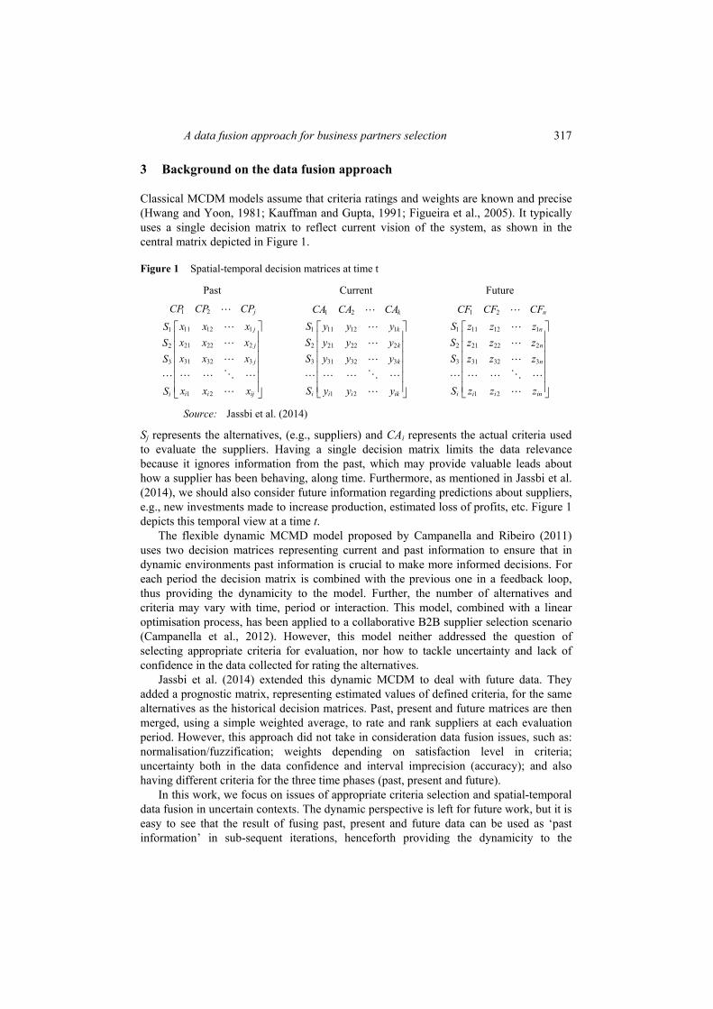
Classical MCDM models assume that criteria ratings and weights are known and precise (Hwang and Yoon, 1981; Kauffman and Gupta, 1991; Figueira et al., 2005). It typically uses a single decision matrix to reflect current vision of the system, as shown in the central matrix depicted in Figure 1.

Figure 1 Spatial-temporal decision matrices at time t

Past Current Future

1 2

11 12 11

21 22 22

31 32 33

1 2

j

j

j

j

i i iji

CP CP CPx x xSx x xSx x xS

x x xS

⎡ ⎤⎢ ⎥⎢ ⎥⎢ ⎥⎢ ⎥⎢ ⎥⎢ ⎥⎣ ⎦

1 2

1 11 12 1

2 21 22 2

3 31 32 3

1 2

k

k

k

k

i i i ik

CA CA CAS y y yS y y yS y y y

S y y y

⎡ ⎤⎢ ⎥⎢ ⎥⎢ ⎥⎢ ⎥⎢ ⎥⎢ ⎥⎣ ⎦

1 2

1 11 12 1

2 21 22 2

3 31 32 3

1 2

n

n

n

n

i i i in

CF CF CFS z z zS z z zS z z z

S z z z

⎡ ⎤⎢ ⎥⎢ ⎥⎢ ⎥⎢ ⎥⎢ ⎥⎢ ⎥⎣ ⎦

Source: Jassbi et al. (2014)

Sj represents the alternatives, (e.g., suppliers) and CAi represents the actual criteria used to evaluate the suppliers. Having a single decision matrix limits the data relevance because it ignores information from the past, which may provide valuable leads about how a supplier has been behaving, along time. Furthermore, as mentioned in Jassbi et al. (2014), we should also consider future information regarding predictions about suppliers, e.g., new investments made to increase production, estimated loss of profits, etc. Figure 1 depicts this temporal view at a time t.

The flexible dynamic MCMD model proposed by Campanella and Ribeiro (2011) uses two decision matrices representing current and past information to ensure that in dynamic environments past information is crucial to make more informed decisions. For each period the decision matrix is combined with the previous one in a feedback loop, thus providing the dynamicity to the model. Further, the number of alternatives and criteria may vary with time, period or interaction. This model, combined with a linear optimisation process, has been applied to a collaborative B2B supplier selection scenario (Campanella et al., 2012). However, this model neither addressed the question of selecting appropriate criteria for evaluation, nor how to tackle uncertainty and lack of confidence in the data collected for rating the alternatives.

Jassbi et al. (2014) extended this dynamic MCDM to deal with future data. They added a prognostic matrix, representing estimated values of defined criteria, for the same alternatives as the historical decision matrices. Past, present and future matrices are then merged, using a simple weighted average, to rate and rank suppliers at each evaluation period. However, this approach did not take in consideration data fusion issues, such as: normalisation/fuzzification; weights depending on satisfaction level in criteria; uncertainty both in the data confidence and interval imprecision (accuracy); and also having different criteria for the three time phases (past, present and future).

In this work, we focus on issues of appropriate criteria selection and spatial-temporal data fusion in uncertain contexts. The dynamic perspective is left for future work, but it is easy to see that the result of fusing past, present and future data can be used as ‘past information’ in sub-sequent iterations, henceforth providing the dynamicity to the


approach. More details about the spatial temporal fusion method are discussed in the next section.

3.1 Data fusion in uncertain contexts

Merging past information with present information and prediction for future trends (or forecasts) may improve the quality of the decision making process, but it is not a risk free process. There are various types of uncertainty that may hamper any decision making process. Roy et al. (1986) distinguish between three types of uncertainty:

1 Imprecision (associated with the difficulty of determining the score of an alternative on a criterion, due to the absence of relevant information or the inability of a decision maker to express his preferences in a consistent way).

2 Stochastic uncertainty.

3 Indetermination (associated to criteria definition and its interpretation).

Moreover, according to Dutta (1985), imprecision can arise from a variety of sources: incomplete knowledge, inexact language, ambiguous definitions and measurement problems, among others.

Models for supplier selection frequently lack support for dealing with imprecision, assuming that precise data and preferences are available (De Boer, 2001). This assumption may lead to erroneous decisions, particularly in evolving and fast changing global markets environments. On the other hand, when more evaluation parameters are used, along with extended datasets, we may be introducing more imprecision in the decision process, even if criteria is clearly defined and indetermination is avoided. Imprecision may be intrinsic due to the nature of the selected evaluation parameters, such as estimations and/or subjective supplier evaluation parameters and also by the imprecise human reasoning.

Fuzzy logic (Zadeh, 1965) has been successfully used to help handle imprecision in decision making processes, particularly in MCDM models (Ribeiro, 1996; Amid et al., 2009; Wang and Yang, 2009; Tzeng and Huang, 2011; Elahi et al., 2011; Seifbarghy et al., 2011; Pang and Bai, 2011; Ozkok and Tiryaki, 2011).

In this work, as mentioned before, we combine a data fusion multicriteria (MCDM) paradigm (Ribeiro et al., 2013) with a temporal model (Jassbi et al., 2014), which, in a dynamic way, integrates historical, present and future information, to support supplier selection. Furthermore our approach includes a different fuzzification technique (Varela and Ribeiro, 2003) for the criteria and also identifies appropriate criteria, for supplier selection, following advices from the literature (Ellram, 1990; Zwick and Wallsten, 1989; Monczka, 2005; Bailey et al., 2008; Lysons and Farrington, 2006; Jassbi et al., 2014).

Our approach works as follows. Different evaluation criteria may be defined for current, past and historical information and fuzzy sets are used to normalise and enable comparison between alternatives. Individual criterion may be adjusted to reflect specific needs. For example, a ‘good price’ may be defined as a price p ∈ [min(D) – y%, min(D) + z%], when comparing prices from different suppliers (domain D). Different membership functions may be used depending on the scenario.


To generate a ranked list of suppliers for each temporal evaluation (past, present and future) it uses mixture operators with weighting functions (Pereira and Ribeiro, 2003), which allows to define relative importance for each criterion, using a qualitative scale. Further, while evaluating the suppliers we may have different levels of confidence on the data, depending on its availability for each criterion. For example, a price proposed by a supplier is a value with no associated uncertainty; hence the confidence is 100%. On the other hand, portfolio rating value may be the result of a more subjective evaluation and we consider a confidence value lower than 100% to express this lack of confidence on the estimated value. Additionally, predicted values may also have lower confidence levels, if it is not clear they identify future trends. Finally, by aggregating the final scores of each temporal evaluation (past, present and future); we obtain a rating for each alternative. The final ranked list of suppliers will support the company business strategic decision or partner selection.

In Sections 4 and 5, a complete illustrative example discusses, step-by-step, the details of the approach proposed in this article.

4 Problem context: partner and supplier selection

Partner and supplier selection is of critical importance in a wide range of business scenarios. This is particularly true when a group of companies is aiming to inter-connect their business activities in the context of collaborative networks (Camarinha-Matos and Afsarmanesh, 2006). The need to implement an agile decision process adds to the overall objective of the supplier selection process, which is to reduce risk, maximise the overall buyer’s value and build long-term relationships between buyers and suppliers (Monczka et al., 1998). All companies that depend on external suppliers for material and component delivery need to continuously evaluate their suppliers, since the quality of the deliveries has a very significant impact on the final quality of the product (Krause and Ellram, 1997).

In order to support the automatic selection of suppliers based on received answers to quotation requests, a system needs to handle multiple variables that may impact the quality of future deliveries and associated cost/benefit ratio. Additionally, it is important to evaluate the historical information about the supplier performance, since it may express a pattern for future deliveries. Prediction of future information should also be included in the decision process, since its aggregation with present and past results may provide a richer view of the supplier capabilities, now and in the near future. Finally, in some situations, the suppliers that are eligible to receive the RFP/RFQ must comply to specific regulations associated with the business scenario.

4.1 Choosing criteria for historical information

The importance of considering historic information on a partner/supplier selection process is clearly demonstrated by Monczka et al. (2005), regarding qualitative factors to enable a wider performance evaluation:

Each criterion above requires some sort of prior knowledge about the partners/suppliers, i.e., information about their past behaviour. Further, the data necessary


to support the definition of each criterion satisfaction level may vary in terms of availability, integrity and quality. Obviously, when considering new suppliers/partners past behaviour is not available and in this case there will be no historical data at time T0, but after that, in any dynamic recurrent process, there will be historic data at T1.

To better clarify the importance of considering historic information in a dynamic decision process let’s assume a buying company is trying to select one out of two possible service providers (suppliers) and the evaluation criteria are: price, delivery time and lead time. Further, the buyer has historical information associated with both suppliers, including detailed information about their orders during the last 12 months. Now, let us consider the following scenario: suppliers S1 and S2 are included as recipients for a RFQ. Both suppliers provided a quote and both quotes had similar price and delivery times. The lead time proposed by both customers is two days. The buyer has historical information about past orders that were fulfilled by both S1 and S2. Let O(i, Sj) be the number of orders delivered by supplier j during month i. Considering that last year the sum of monthly supplied orders is similar for S1 and S2, we have:

1 12 1 12

( , 1) ( , 2)i i

O i S O i S≤ ≤ ≤ ≤

=∑ ∑

We will also assume that all provided services have adequate quality and completely fulfil the buyer’s requirements. Lack of quality during the last 12 months is inexistent but some services were provided with delays. Those delays were registered in a database as the number of days passed since the delivery time proposed in the purchase order. The total number of days associated with the delays is similar for both suppliers. Let n be the number of orders fulfilled by supplier 1; m the number of orders fulfilled by supplier 2; and D(Oi, Sj) the number of days order i was delayed by supplier j.

This illustrative scenario could lead us to assume both suppliers would be a good choice, since all criteria is evaluated equally. But this assumption may be incorrect if we consider the historic information about previous orders during the last 12 months, for S1 and S2 in Table 3.

According to the historical information in Table 3, we have similar behaviour for the number of orders and the number of delays for S1 and S2, as follows:

1 12 1 12

1 1

( , 1) ( , 2) 72

( , 1) ( , 2) 45i i

i n i m

O i S O i S

D Oi S D Oi S≤ ≤ ≤ ≤

≤ ≤ ≤ ≤

= =

= =

∑ ∑∑ ∑

However, if we observe the remaining items from Table 3, it is clear that there is a significant difference in the average number of delayed days per order (1.56 for S1 vs. 0.94 for S2). These values suggest that S1 would be a better choice. Continuing, if we analyse the other items, we can also clearly see that there is performance degradation for supplier S2. On the other hand, supplier S1 was able to completely mitigate all delays in seven months, while, at the same time, increasing the number of fulfilled orders significantly. This past information analysis is displayed graphically in Figure 2. Taking this information into account, a manager would probably decide to assign the order to supplier S1, since it is a more secure choice for minimising the risk of delays.


Table 2 Qualitative factors to enable a wider performance evaluation

Criterion Description

Problem resolution ability Supplier’s attentiveness to problem resolution. Technical ability Supplier’s manufacturing ability compared with other industry

suppliers. Ongoing process reporting Supplier’s ongoing reporting of existing problems or

recognising and communicating a potential problem. Corrective actions response Supplier’s solutions and timely response to requests for

corrective actions, including a supplier’s response to engineering change request.

Supplier cost-reduction ideas Supplier’s willingness to help find ways to reduce purchase cost Supplier new-product support

Supplier’s ability to help reduce new- product development cycle time or to help with product design.

Buyer/seller compatibility Subjective rating concerning how well a buying firm and a supplier work together.

Source: Monczka et al. (2005)

Table 3 Historic information for suppliers

Month 1 2 3 4 5 6

S1 10 10 10 5 5 5 Delivery delays (number of days) S2 0 0 0 0 4 4 S1 2 2 2 4 4 4 Number of fulfilled orders S2 10 10 10 10 4 4 S1 5 5 5 1.25 1.25 1.25 Delays per order (average, in days) S2 0 0 0 0 1 1 S1 1 1 1 2 2 3 Delayed orders S2 0 0 0 0 1 1 S1 50 50 50 50 50 25 On time delivery performance S2 100 100 100 100 75 75 S1 100 100 100 100 100 100 Defect free delivery S2 100 100 100 100 100 100

Month 7 8 9 10 11 12

S1 0 0 0 0 0 0 Delivery delays (number of days S2 4 4 5 8 8 8 S1 8 8 8 10 10 10 Number of fulfilled orders S2 4 4 4 4 4 4 S1 0 0 0 0 0 0 Delays per order (average, in days) S2 1 1 1.25 2 2 2 S1 0 0 0 0 0 0 Delayed orders S2 1 1 1 2 2 2 S1 100 100 100 100 100 100 On time delivery performance S2 75 75 75 50 50 50 S1 100 100 100 100 100 100 Defect free delivery S2 100 100 100 100 100 100


Only considering the static nature of criterion such as ‘on time delivery’ and ‘defect delivery’ is insufficient to support a solid decision. Knowing how the supplier performs during a reference period is important to detect positive or negative performance trends. These trends may reflect a decision risk. A positive evolution of the ‘on time delivery’ criterion means that the number of delayed orders is being minimised during that period. The same happens with the quality criterion ‘defect free delivery’. A positive performance over time on that criterion implies that the number of orders with defects or that does not fulfil the purchase order requirement is being minimised.

Figure 2 Comparison of trends from past behaviours for S1 and S2 (see online version for colours)

These positive and negative evolution trends must be taken into account in the dynamic decision process. Therefore, suppliers’ trends should be used to:

1 estimate future trends

2 add additional criteria to penalise bad performance evolution in the past.

If estimation/prediction includes reliable results in a given scenario, poor performance patterns in the past will impact the forecasted performance. This will be enough to differentiate between suppliers with similar global criterion values, such as on time delivery and defect free delivery, but with different performance evolution records.

In summary, historical information is in fact quite important to support more informed decisions. Furthermore, criteria associated with historical information should include parameters allowing the decision maker to understand if the performance evolution is positive or negative.

4.2 Choosing criteria for prediction

Ellram (1990) highlights the need for considering traditional criteria (price, delivery time, etc.) and also longer term and quality criteria such as, strategic fit and future manufacturing capabilities. Knowing more about future manufacturing capabilities and customer demand forecasts may help support better strategic decisions. Further, having access to predicted information about suppliers may be essential for decisions that


involve possible future events (Zwick and Wallsten, 1989). Many decisions in a company are strategic decisions for the future and they may turn out to be unrealistic if they lack considering past behaviours and future information about suppliers (Jassbi et al., 2014).

Forecasting (or prediction) may be an important tool for the company strategic and operational planning. Lysons and Farrington (2006) consider forecasting the basic ingredient for planning and decision making processes. Bailey et al. (2008) point out three typical causes of failure for forecasting information:

1 The perceived evolution pattern is not continued into the future.

2 The past pattern has not been adequately understood.

3 Random fluctuations have prevented the pattern from being recognised.

To avoid the above causes, careful analysis should be performed to minimise errors caused by incorrectly identifying evolution trends or patterns. There are several qualitative techniques to predict future behaviour, including identifying trends and dominant opinions, such as the Delphi technique, expert judgement and test marketing (Dalkey and Helmer, 1963; Basu and Schroeder, 1977; Rescher, 1997). On the other hand, there are quantitative techniques using numerical data to predict the evolution of temporal series based on past information, such as moving averages and exponentially weighted average methods, autoregressive-moving-average (Whittle, 1951), autoregressive integrated moving average (Mills, 1990), Kalman (1960) filter, exponential smoothing (Brown, 1956), extrapolation (Armstrong, 1984), linear prediction (Makhoul, 1975) and trend estimation among (Bianchi et al., 1999), among other methods.

In this work, since we only analyse two simple scenarios in an illustrative case, we use expert knowledge (from the authors) to determine forecasting values for the next business year. Any other forecasting method could have been used, depending on the specific characteristics of the business scenario.

5 A data fusion approach for partner’s selection

The proposed approach intends to be used in the context of supplier and partner evaluation processes in collaborative networks, including VO/VE and standard partner networks with supply chain integration. The main aims of the approach are:

a Fully support the decision making process based on spatial-temporal different criteria.

b Use a temporal model including information in terms of time (past, present and future information).

c Support imprecision and lack of confidence on available data by using fuzzy logic for criterion evaluation.

d Allow different relative importance (weights) for different temporal stages and also dependent on criteria satisfaction by penalising or rewarding them.


5.1 Main steps of the proposed approach

Figure 3 depicts the six steps associated with the proposed approach for suppliers/business partner’s evaluation:

5.1.1 Create past, present and future evaluation matrices

As mentioned before, in the proposed approach three different matrices must be defined when the process starts: past, present and future (Jassbi et al., 2014). In Section 2.1, we discussed the main criteria (attributes) that could be considered when evaluating suppliers and business partners, therefore, here we just address the key factors of choosing criteria for the three matrices in the context of VO/VE.

Figure 3 Overview of the spatial-temporal supplier evaluation approach (see online version for colours)

DEFINE EVALUATION CRITERIA

ORGANIZE HISTORICAL INFORMATION

ORGANIZE FUTURE INFORMATION

SUBMIT RFP/RFQ

RECEIVE PROPOSALS/QUOTES

EVALUATE SUPPLIERS

SELECT SUPPLIER

CREATE PAST, PRESENT AND FUTURE EVALUATION

MATRICES

FUZZIFY EACH CRITERION

FUSION: CRITERIA AGGREGATION

DECISION

FILTER UNCERTAINTY

APPLY CRITERIA WEIGHTS

The initial past matrix is built using historical information regarding the supplier’s performance. Past criteria satisfaction values may be obtained from information stored in a database, which may belong to the buyer, VE/VO or even the VBE to which both buyer and sellers belong. When analysing information about the past, parameters such as delivery time and lead time may not be important, since the company may be using historical information about previous orders with different constraints. In this case, price, on time delivery performance and defect delivery rates will be more useful.

When evaluating the present status, data included in the received quotes/proposals is of utmost importance. This may include price, lead and delivery times and other specific data. This information may be aggregated with quality and delivery performance rates, thus allowing taking risk into account in the decision making process.


Finally, to build the future evaluation matrix, some prediction must be defined to obtain future information about the candidate partners. The prediction may target criterion such as performance indexes and prices, making assumptions about future values from past performance patterns or investments, (e.g., quality, managerial processes, technology). In this case, performing prediction on parameters such as delivery time may be considered irrelevant, since they depend on production capacity availability from suppliers, quantity of each product that was requested in each order and so on. On the other hand, if the orders are fairly standardised, this parameter may become relevant, since different values of delivery time for similar orders may define a performance pattern that may produce relevant forecasts.

The next sections present the details of the approach fusion steps:

1 normalise the criteria using fuzzification

2 filter uncertainty

3 define criteria weights

4 fusing information by aggregating criteria

5 final ranking.

5.1.2 Normalisation process: fuzzify each criterion

Existing data (values) for all criteria must be normalised before any fusion process may occur (Ribeiro et al., 2013). Normalisation is essential to guarantee that values are numerical and comparable, to enable being aggregated. Just dividing a value by the maximum existing value (when high values are good, such as quality index) or by the minimum (when low values are good, such as price) is a fast way to normalise the respective decision matrix (Jassbi et al., 2014), but lacks any semantic interpretation to properly express concepts such as ‘lower is better’.

Hence, in this work, we propose using a fuzzification process to normalise the data, based on simple triangular membership functions to represent the acceptable criterion values (Varela and Ribeiro, 2003) for ‘lower is better’ and ‘higher is better’:

0,

lower is better : ( ) 1

1,

i i

ii i i

i

i

if x b px bμ x if b x b p

pif x b

⎧ > +⎪ −⎪= − < ≤ +⎨⎪⎪ ≥⎩

(1)

{

0,

higher is better : ( ) 1 ,

1,

i i

ii i i

i

i

if x b px bμ x if b p x b

pif x b

< −−= − − ≤ <

≥

(2)

The membership functions may be adjusted for each criterion and also for the past, present or future evaluation processes. In the illustrative examples, we use these membership functions, because all expected criteria fits in the ‘lower is better’ and ‘higher is better’ categories.


After the fuzzification process we will have three updated matrices, where the cell’s values (functions 1 and 2) were substituted by the respective membership value, µ(x).

5.1.3 Filter uncertainty

All information gathered about the criteria level of achievement may have embedded uncertainty, due to lack of precision while gathering data, insufficient data to build required indexes and lack of confidence in the quality of data for specific criteria, among other possible causes.

In order to filter uncertainty we will use the method proposed in Pais et al. (2010) and Ribeiro et al. (2013), which considers two parameters, accuracy and confidence to ‘filter’ the membership function values. The first parameter expresses deviations from nominal values and the second expresses the degree of trust on the data gathered. The logic of this filtering process is that if we do not trust an input source, (e.g., confidence on data is only 80%) then the initial value must decrease proportionally, (e.g., a value ten would be reduced to eight). The accuracy encompasses considering deviations, such as, for example +3 or –3 from a value of ten.

Let aij be the accuracy associated with criterion j for supplier i, which represents a left or right deviation from the original value. When aij is zero it means we accept the gathered value without deviation errors. The confidence, wcj, is a percentage, as for example, we trust with 90% the values for ‘on time delivery performance’. Additionally, λ ∈ [0, 1], is a parameter that reflects the decision maker’s attitude. Values close to zero indicate an optimistic attitude; higher values indicate a pessimist attitude. Hence, the adjusted membership value is calculated using the following formula (Ribeiro et al., 2013):

( ){ } ( )[ , ]

*(1 * max ( ) *ij j j ijx a b

fu wc λ μ x μ xi μ x∈

= − − (3)

where [a, b] is the inaccuracy interval:

min( ), min( ) min( )

, max( )max( ), max( )

ij ij

ij ij ij ij

ij ij ij ij

ij ij

D if x a Da

x a if x a D

x a if x a Db

D if x a D

− ≤⎧= ⎨ − − >⎩

+ + ≤⎧= ⎨ + >⎩

Using this function we are able to penalise input values, which display any of the two types of uncertainty, i.e., inaccuracies or lack of confidence on data, within an optimist or pessimist view from the decision maker.

5.1.4 Apply criteria weights

Following the work of Ribeiro et al. (2013), we now need to define the weighting functions. Here we will use linear weighting functions to express the relative importance of criteria. These functions allow penalising or rewarding bad or good levels of criteria satisfaction, i.e., instead of assigning single weights, we represent them using a function that depends on criteria satisfaction (Ribeiro and Pereira, 2003).


( ) 1* , 0 , 1

1ij

ijfu

L fu a+

= ≤ ≤+β α β

β (4)

where α defines the semantic importance of criteria, according to Table 4 and the β parameter defines the slope for the weighting function (a higher value means a steeper function) to penalise, more or less, badly satisfied criteria, as shown in Table 5.

For example, if we assign to criterion price the values α = 1 and β = 0.67, we are defining price as a ‘very important’ evaluation parameter with an average slope decrease. In this example, we want to reward the best quotes and penalise the bad ones, (i.e., we want to reward lower prices). Table 4 Semantic importance of criteria

α Meaning

1 Very Important 0.8 Important 0.6 Average importance 0.3 Low importance 0.1 Very low importance 0 Ignored

Table 5 Slope for the weighting criteria

β Meaning

1 High slope – higher penalty 0.67 Medium slope – average penalty 0.33 Low slope – low penalty 0 Null

5.1.5 Fusion: criteria aggregation

At this stage we should already have the three matrices with their respective cells values, (fuij), for each existing criterion, per alternative supplier, for the three temporal periods (past, present and future).

Since we may have different criteria for each stage, we need to aggregate them to obtain the resulting vectors for past, present and future scores, per supplier.

We will use the aggregation method proposed by Ribeiro et al. (2013), which is based on the mixture of operators with weighting functions (Pereira and Ribeiro, 2003) as follows:

( )( )

1

*iji ijn

ijk

L fur sum fu

L fu=

⎛ ⎞⎜ ⎟= ⎜ ⎟⎜ ⎟⎝ ⎠∑

(5)

where fuij is the filtered value for criteria j and supplier i and L(fuij) is the corresponding weighted value.


After executing this step for the three time periods we obtain the ratings for past, present and future information per supplier.

5.1.6 Decision

After having fused the values associated with each criterion for the three types of matrices (past, present and future) we are now able to use the dynamic spatial-temporal process (Jassbi et al., 2014; Campanella and Ribeiro, 2011) for obtaining the final rating for suppliers. Figure 4 formalises the three vectors and the final aggregated vector (decisional rating), as follows:

Figure 4 Past, present, future and aggregated vectors

Past Current Future Final decision

11

12

13

ii

Past ratePSPSPS

PS

⎡ ⎤⎢ ⎥⎢ ⎥⎢ ⎥⎢ ⎥⎢ ⎥⎢ ⎥⎣ ⎦

11

12

13

ii

P rateaSaSaS

aS

−

⎡ ⎤⎢ ⎥⎢ ⎥⎢ ⎥⎢ ⎥⎢ ⎥⎢ ⎥⎣ ⎦

11

12

13

ii

F ratefSfSfS

fS

−

⎡ ⎤⎢ ⎥⎢ ⎥⎢ ⎥⎢ ⎥⎢ ⎥⎢ ⎥⎣ ⎦

1 1 1 1

2 2 2 2

3 3 3 3

i i i i

DecisionS P a fS P a fS P a f

S P a f

⊗ ⊗⎡ ⎤⎢ ⎥⊗ ⊗⎢ ⎥⎢ ⎥⊗ ⊗⎢ ⎥⎢ ⎥⎢ ⎥⊗ ⊗⎣ ⎦

where ⊗ represents an aggregation operator such as the weighted average or any other operator. For example, if we use a weighted average we can consider that past information is more relevant than future one and assign more weight to these temporal-criteria than to the future one. Again, any other operator from geometric mean, parametric operators could be used for determining the final evaluation for each supplier.

In summary, the vectors are combined and the result will be a single vector with a single score per supplier, which after ordered will provide the ranking of all suppliers. The resulting vector provides more reliable information for the buyer to select the best suppliers or business partners, since it reflects the supplier’s past, current and future expected behaviours. Obviously, the final ratings are greatly influenced by the chosen criteria, the defined weights and confidence and accuracy values considered. The buyer company may adjust these parameters, according to the specificities of its business scenario.

5.2 Examples in practice

In the following sections we illustrate the application of the proposed approach using two different business network scenarios.

5.2.1 Service procurement

Let us consider a scenario of service outsourcing to illustrate the application of the proposed model. Company A is focused on interactive projects, operating globally in several different sectors. The company is currently receiving a lot of enquiries for interactive software solutions. The number of assigned orders is increasing exponentially and the company is unable to fulfil new requests by itself, since its internal teams are almost fully allocated to current projects. The company aims to be a reference


international player in interactive projects and to achieve this it needs to demonstrate capacity to fulfil all orders.

Company A has just received a request from a major international brand that needs a customised software solution for its retail store network. The business potential is very high according to the sales team. Based on that information, the company starts evaluating the best quote it can provide and how it will be able to fulfil the project requirements. The project management office director considers that he will be able to assign some of its software developers, who are currently working on another project, by negotiating a delivery deadline with one existing customer. This will allow the company to develop the software solution internally. However, for working in the project design, a key component for the required solution, it will not be possible to free any of its internal designers from their current assignments.

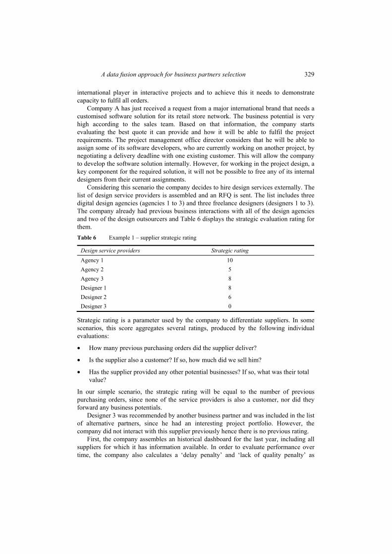
Considering this scenario the company decides to hire design services externally. The list of design service providers is assembled and an RFQ is sent. The list includes three digital design agencies (agencies 1 to 3) and three freelance designers (designers 1 to 3). The company already had previous business interactions with all of the design agencies and two of the design outsourcers and Table 6 displays the strategic evaluation rating for them. Table 6 Example 1 – supplier strategic rating

Design service providers Strategic rating Agency 1 10 Agency 2 5 Agency 3 8 Designer 1 8 Designer 2 6 Designer 3 0

Strategic rating is a parameter used by the company to differentiate suppliers. In some scenarios, this score aggregates several ratings, produced by the following individual evaluations:

• How many previous purchasing orders did the supplier deliver?

• Is the supplier also a customer? If so, how much did we sell him?

• Has the supplier provided any other potential businesses? If so, what was their total value?

In our simple scenario, the strategic rating will be equal to the number of previous purchasing orders, since none of the service providers is also a customer, nor did they forward any business potentials.

Designer 3 was recommended by another business partner and was included in the list of alternative partners, since he had an interesting project portfolio. However, the company did not interact with this supplier previously hence there is no previous rating.

First, the company assembles an historical dashboard for the last year, including all suppliers for which it has information available. In order to evaluate performance over time, the company also calculates a ‘delay penalty’ and ‘lack of quality penalty’ as


previously described. Table 7 summarises the criteria used to analyse historical information. Table 7 Example 1 – supplier ratings (based on historical information)

Cost per hour (average)

On time delivery performance

Delay penalty

Quality rating

Lack of quality penalty

Design service providers CPH OTD DP QR LQP Agency 1 75.50 95% 10.00 100% 0.00 Agency 2 79.00 90% 5.00 98% 2.00 Agency 3 72.50 95% 15.00 95% 6.00 Designer 1 37.50 80% 20.00 80% 10.00 Designer 2 45.00 78% 25.00 85% 15.00

Second, current data is normalised (fuzzified) using the triangular functions described in Section 5.1.3. The ‘lower is better’ membership function is used for ‘cost per hour’, ‘delay penalty’ and ‘lack of quality penalty’. ‘Higher is better’ membership function is used for ‘on time delivery performance’, ‘quality rating’ and ‘portfolio rating’. The resulting membership values for all criterions are shown in Table 8. Table 8 Example 1 – membership values for each current data criterion

CPH OTD DP QR LQP xi1 u(x)

xi2 u(x)

xi3 u(x)

xi4 u(x)

xi5 u(x)

75.5 0.084 95% 1.000 10 0.750 100% 1.000 0 1.000 79 0.000 90% 0.706 5 1.000 98% 0.900 2 0.867 72.5 0.157 95% 1.000 15 0.500 95% 0.750 6 0.600 37.5 1.000 80% 0.118 20 0.250 80% 0.000 10 0.333 45 0.819 78% 0.000 25 0.000 85% 0.250 15 0.000

The third step is to filter the uncertainty from the results. For this filtering the company considers individual confidence levels for each criterion, except for ‘cost per hour’ and ‘on time delivery performance’ because they are based on existing data and have no associated uncertainty. ‘Delivery penalty’ and ‘lack of quality penalties’ is estimates based on possible evolution trends and as such, they have lower confidence values. Quality rating could be a subjective evaluation, performed by different project managers after provided services. Table 9 Example 1 – filtered values using defined accuracy and confidence current values

wcj 50% λj 1 Accuracy 5% pi 20,000 i, j µ(xij) xij aij a u(a) b u(b) uij 1, 3 0.750 10.000 0.500 9.500 0.775 10.500 0.725 0.3656 2, 3 1.000 5.000 0.250 5.000 1.000 5.250 0.988 0.5000 3, 3 0.500 15.000 0.750 14.250 0.538 15.750 0.463 0.2406 4, 3 0.250 20.000 1.000 19.000 0.300 21.000 0.200 0.1188 5, 3 0.000 25.000 1.250 23.750 0.063 25.000 0.000 0.0000


Next, an accuracy rate, expressing the allowed deviation from the base values, is defined for each criterion, based on the associated data quality. The value also reflects the imprecision associated with the data gathering process. Based on the criteria and its associated confidence rates, the filtered imprecision values, f(uij), were calculated. Table 9 illustrates the calculations performed for the delay penalty criterion for historical information.

After calculating the filtered value for each criterion, the fourth step is to determine the corresponding weighted rating, according to equation (4), using the parameters defined in Table 4 and Table 5 for the weighting functions. Table 10 depicts the chosen parameters for past information. Table 10 Example 1 – parameters for each criterion weighting function for past, current and

future

Criterion (j) CPH OTD DP QR LQP

Confidence for historic criteria

100% 100% 50% 50% 30%

1 0.8 0.6 0.8 0.8 α (Table7) Very important Important Average importance Important Important

1 0.67 0.67 0.67 0.67 β (Table 8) High slope Medium

slope Medium slope Medium

slope Medium

slope

An illustration of the calculated weighted rating (4), for CPH is shown in Table 11. Table 11 Example1 – CPH weights

i, j fuij α β L(fuij)

1, 1 0.0843 1 0.670 0.5422 2, 1 0.0000 1 0.670 0.5000 3, 1 0.1566 1 0.670 0.5783 4, 1 1.0000 1 0.670 1.0000 5, 1 0.8193 1 0.670 0.9096

Table 12 Example 1 – matrix with future information data

i ri Supplier 1 0,4998 Agency 1 2 0,3749 Agency 2 3 0,4303 Agency 3 4 0,3979 Designer 1 5 0,2906 Designer 2 6 0,0000 Designer 3

After these four steps we have a weighted vector for each criterion. The final step (five) is to calculate the final score (rating) for each supplier. Table 12 shows the results obtained for historic information, using the data fusion process equation (5). Observing


Table 12, agency 1 is best choice for new assignments, followed by agency 3. Since designer 3 did not fulfil any previous orders, its past score is zero.

Next, we repeat the process for future information. Prediction may be performed using expert judgement or quantitative methods (forecasting), such as moving linear averages, quadratic averages and other techniques. Here we assume our prediction for future information is the data depicted in Table 13. Since we do not have historical data about designer 3, we will not include him on the forecast.

The managers have a low confidence regarding values resulting from prognostics because they are estimated values. Predicting the evolution of portfolio rating may be considered a risky (although valuable) process, hence, the associated criterion is assigned a low confidence value (35%). Using the same steps of the historic data fusion, we obtain the results for fused prognostic information, as shown in Table 16. Table 13 Example 1 – matrix with future information data

Cost per hour (average)

On time delivery performance (estimated)

Quality performance (estimated)

Portfolio rating (estimated)

Design service providers

CPE OTDE QPE PRE Agency 1 82.50 98% 100% 90% Agency 2 95.00 95% 98% 80% Agency 3 80.00 98% 98% 85% Designer 1 50.00 85% 85% 75% Designer 2 55.00 90% 90% 80%

Having calculated the historical and prediction scores for each alternative, we now need to evaluate the present status. This means evaluating the proposals/quotes that have been received and then fusion the respective information. The chosen criteria description is shown in Table 14. Table 14 Criteria used for current service procurement example

Quoted price QP

The cost of required goods/services.

Total time to deliver TTD

The sum of the lead time and the delivery time proposed by supplier. Corresponds to the total amount of time, starting from order date, until all services have been supplied.

Portfolio rating

This rating evaluates the quality of the company portfolio on projects similar to the ones that are being procured. It results from a subjective evaluation, so it has a low confidence level assigned to it.

Supplier relation rating

This rating grades the strategic importance suppliers, e.g., a supplier that is simultaneously a customer may have a higher rating than a standard supplier. Here we consider the number of previous orders assigned to the supplier and a supplier with a closer relationship will have higher priority than a supplier without previous relationship with the company.

Table 15 depicts the set of quotes (current data) received from the candidate partners and also the portfolio rating and supplier relation rating that were assigned by the company.


Table 15 Example 1 – supplier current data

Quoted price Delivery time Lead time Portfolio rating Strategic rating Design service providers QP DT LT PR SR

Agency 1 6,040 10 5 100% 10 Agency 2 10,744 17 5 98% 5 Agency 3 10,440 18 4 98% 8 Designer 1 6,150 20 5 95% 8 Designer 2 7,920 22 10 80% 6 Designer 3 6,000 8 2 100% 0

Table 16 Example 1 – results for historical, present and prognostic evaluations

Historical Present Future

Supplier Score Supplier Score Supplier Score Agency 1 0.4998 Agency 1 0.8562 Agency 1 0.1733 Agency 3 0.4303 Designer 3 0.8507 Agency 3 0.1414 Designer 1 0.3979 Designer 1 0.6804 Designer 2 0.1277 Agency 2 0.3749 Agency 3 0.5321 Designer 1 0.1011 Designer 2 0.2906 Agency 2 0.4800 Agency 2 0.0752 Designer 3 0.0000 Designer 2 0.4294 Designer 3 0.0000

Table 16 summarises the fused rating values for past, current and future information. Regarding the present (current) evaluation matrix the best option will be agency 1. It is interesting to note that designer 3 provided the quote with the lowest price, lowest delivery and lead times and also has a great portfolio. But the weight assigned to strategic rating has pushed it back to the second place on present score list.

As can be observed in Table 16 there is no consensus about the ranking of the business partners if we only take individual evaluations of past, current or future information, except that agency 1 seems to be the best one in all three iterations. To reach a consensus we used the dynamic spatial-temporal process (Jassbi et al., 2014; Campanella and Ribeiro, 2011), for the approach final step in this paper, i.e., decision step in Figure 3 (ranking alternatives).

We start by defining the relative importance for each evaluation. We consider that current and past information are more important and prediction information is less important (weights depicted in Table 17). Table 17 Example 1 – relative importance of each evaluation

Past Present Future 0.8 1 0.6 α

Important Very important Average importance 0.67 1 0.67 β

Medium slope High slope Medium slope


Next we calculate the weighted values L(fuij) (4) and then we aggregate them to obtain the final score (rating) of each alternative partner. Table 18 Example 1 – final composite score matrix

Supplier Score

Agency 1 0.6013 Designer 1 0.4654 Designer 3 0.4463 Agency 3 0.4102 Agency 2 0.3543 Designer 2 0.3119

Although designer 3 offered the most competitive quote, the lack of previous interactions with it and its low strategic rating pushed him back to third place. Considering the spatial-temporal decision making process, combined with the data fusion process, the selected partner in this illustrative example is agency 1, which is consistent with the individual results shown in Table 16.

5.2.2 Component procurement

For the second example we will borrow the example presented in Jassbi et al. (2014), which refers to a Middle Eastern automotive manufacturing company. Data from this company has been gathered along several years for its six suppliers.

The company evaluates its partners using the following criteria: ‘price of unit’ (POU), ‘on time delivery performance’, ‘defect free delivery’, ‘product variety’ and ‘production capacity’. To further allow the evaluation of historical performance evolution, we will add two criterions: ‘delay penalty’ and ‘lack of quality penalty’, both used to penalise negative trends in both delivery times and quality of deliverables.

Our simulation will be based on the following scenario:

• By the end of 2014, the company issues an RFQ and receives quotes from its six suppliers. Reference date is 01-01-2015.

• The company possesses historical information for all six suppliers during 2012, 2013 and 2014.

• The company can use historical information from 2012 and 2013, along with expert judgement, to predict how the suppliers will probably behave during the following year (2015).

Table 19 depicts the input values for 2014. The fuzzification step is performed and the respective membership value is calculated

for each criterion level of attainment (Table 18), resulting in the normalised matrix in Table 20:

Next, uncertainty will be filtered. The company assigns the confidence level for each criterion to be used in the filtering process of the historical information, as shown in Table 23. Although the company has total confidence in some of the criterion, such as POU, that may not happen with others. For example, production capacity may be a value


shared by potential suppliers when they reply to a RFQ/RFP. The company may consider it to be information which may be manipulated by suppliers in order to get a higher score during evaluation, thus assigning a lower confidence value to this criterion. The confidence level may be used by the company to differentiate criteria based on the quality of the information it typically receives for suppliers or possesses internally. Using those values we build the evaluation matrix for historic data. For example, Table 21 shows how the production capacity evaluation matrix would look like. Table 19 Example 2 – supplier ratings for 2014 (historic)

Price of unit

On time delivery

performance

Delay penalty

Defect free

delivery


Production capacity (monthly)

Product variety Supplier

POU OTD DP DFD LQP PC PV Supplier 1 424,630.00 100% 0 100% 0 24,000 4 Supplier 2 403,398.50 92% 25 98% 10 14,000 5 Supplier 3 433,400.00 100% 0 100% 0 26,000 4 Supplier 4 411,730.00 95% 25 99% 5 16,000 5 Supplier 5 403,490.00 94% 20 97% 6 15,000 3 Supplier 6 395,330.00 92% 22 97% 6 12,000 3

Table 20 Example 2 – membership value for each historic criterion values

POU DP LQP OTD

x u(x)

x u(x)

x u(x)

x u(x) 424,630 0.230 0 1.000 0 1.000 100% 1.000 403,399 0.788 25 0.000 10 0.000 92% 0.000 433,400 0.000 0 1.000 0 1.000 100% 1.000 411,730 0.569 25 0.000 5 0.500 95% 0.375 403,490 0.786 20 0.200 6 0.400 94% 0.250 395,330 1.000 22 0.120 6 0.400 92% 0.000

DFD PC PV x u(x)

x u(x)

x u(x)

100% 1.000 24000 0.857 4 0.500 98% 0.333 14000 0.143 5 1.000 100% 1.000 26000 1.000 4 0.500 99% 0.667 16000 0.286 5 1.000 97% 0.000 15000 0.214 3 0.000 97% 0.000 12000 0.000 3 0.000

The historic matrix is then fused, (i.e., the criteria are aggregated to produce a composite value) and the resulting decision rating vector is depicted in Table 25. If we only use historical information, supplier 1 would be the best choice, followed by supplier 3. Next, we must repeat the process for forecasting values. First, the forecast matrix is built, based on expert judgement and projection of historical patterns, as shown in Table 22.


Table 21 Example 2 – filtered values using defined accuracy and confidence values for historic production capacity

wcj 40% λj 1 (in)Accuracy 5% p 14000 i, j u(xij) xij aij a u(a) b u(b) acij 1, 1 0.857 24,000 1,200 22,800 0.7714 25,200 0.9429 0.313 2, 1 0.143 14,000 700 13,300 0.0929 14,700 0.1929 0.054 3, 1 1.000 26,000 1,300 24,700 0.9071 26,000 1.0000 0.400 4, 1 0.286 16,000 800 15,200 0.2286 16,800 0.3429 0.108 5, 1 0.214 15,000 750 14,250 0.1607 15,750 0.2679 0.081 6, 1 0.000 12,000 600 12,000 0.0000 12,600 0.0429 0.000

Table 22 Example 2 – evaluation matrix for future information

Price of unit

On time delivery

performance

Delay penalty

Defect free

delivery


Production capacity (monthly)

Product variety Supplier

POU OTD DP DFD LQP PC PV Supplier 1 456,100 95% 20 100% 0 30,000 5 Supplier 2 433,295 98% 5 98% 2 18,000 6 Supplier 3 482,990 100% 0 100% 0 31,000 5 Supplier 4 442,500 98% 10 100% 0 18,000 5 Supplier 5 427,000 95% 20 99% 6 20,000 3 Supplier 6 424,620 95% 18 99% 6 18,000 4

In this scenario, we used the same criteria for historical information and for forecasting. The following confidence levels and weights were assigned for the forecasting assumed values. Table 23 Example 2 – individual criterion confidence values and weights for historic present

and prognosis

POU DT OTD DP DFD LQP PC PV

Confidence for historic information

100% 85% 60% 80% 60% 40% 40% 60%

Confidence for present information

100% 90% 80% 90% 80% 90% 90% 80%

Confidence for prognostic 60% 60% 40% 30% 40% 30% 20% 20%

α 1 1 0.8 0.6 0.8 0.6 0.3 0.3

β 0.67 0.67 0.67 0.67 0.67 0.67 0.33 0.33

After performing the fuzzification, filtering the uncertainty and then fusion the considered criteria we get the forecast decision rating vector, as depicted in Table 24.

According to the forecast information, supplier 4 would be the best choice, followed by supplier 3. Finally, the company must consider the quotes it received, to compose the initial current information matrix. In this scenario, three criteria are used and the respective values are shown in Table 24.


Table 24 Example 2 – current data for supplier ratings according to quotes

Price of unit Delay time Lead time Extended DT Supplier

POU DT LT DT + (max (LT-d*), 0) Supplier 1 364,300 100 5 105 Supplier 2 346,085 120 5 125 Supplier 3 375,600 85 10 95 Supplier 4 356,820 90 15 90 Supplier 5 349,680 100 10 100 Supplier 6 339,160 115 10 125

Notes: *d is the number of days until the order will be assigned. In this scenario, the company wants to order right now, so d = 0.

After performing the fuzzification, uncertainty filtering and the fusion phases, we obtain the rating vector for present/current information, as shown in Table 25. Supplier 4 is the best option, followed by supplier 5. Table 25 Example 2 – historical, present and future results

Historical Present Future Supplier Score Supplier Score Supplier Score Supplier 1 0.576040 Supplier 4 0.764267 Supplier 4 0.269561 Supplier 3 0.553253 Supplier 5 0.712656 Supplier 3 0.262399 Supplier 6 0.345866 Supplier 6 0.676113 Supplier 2 0.227191 Supplier 4 0.327206 Supplier 2 0.529615 Supplier 1 0.212573 Supplier 5 0.300024 Supplier 3 0.515420 Supplier 6 0.185148 Supplier 2 0.273615 Supplier 1 0.441497 Supplier 5 0.171979

Again, since there is no consensus on the three matrices for the three time iterations, we will apply the dynamic multicriteria process (Jassbi et al., 2014) using different weights, to express the relative importance the company places in the temporal information (past, current or forecast). This is the final step of our approach (decision step, Section 5.1.6). The confidence and relative importance for the weighting functions for each periodic information is shown in Table 26. Table 26 Example 2 – relative importance of each evaluation vector

Criterion (j) Past Present Future

Confidence 100% 100% 90% 0.8 1 0.6 α

Important Very important Average importance 0.67 1 0.67 β

Medium slope High slope Medium slope

From these semantic weights, we calculate the respective weighted values L(fuij) as shown in Table 27. Finally by fusing the three vectors above, (i.e., aggregating the criteria values) it is produced the final composite decision ranking vector (Table 28).


Table 27 Example 2 – weighted values

i ri Past ri Present ri Future 1 0.209 0.185 0.046 2 0.086 0.243 0.052 3 0.194 0.221 0.058 4 0.099 0.368 0.059 5 0.092 0.345 0.036 6 0.109 0.320 0.039

After performing all the steps of the proposed approach, we observe that supplier 4 is the best choice, followed by supplier 3, when fusing historical information, current quotes and forecasting. Supplier 1, the one with the higher rating according to historical information, drops to 5th place due to poor results with present and forecast information. It is interesting to see that in this final scoring the first classified is the same as the one (S4) obtained when analysing only present information; however, S3 is the second classified while in the current information it was S1. This scenario clearly demonstrates the importance of spatial-temporal knowledge in informed decision-making, as well as highlights the dynamic nature of most decision processes, particularly in supplier selection. Table 28 Example 2 – final composite scores

Supplier Score Supplier 4 0.51822 Supplier 3 0.47075 Supplier 5 0.46486 Supplier 6 0.46151 Supplier 1 0.43891 Supplier 2 0.37476

6 Conclusions

In this paper, we discussed a dynamic multicriteria decision making approach, which uses data fusion and a spatial-temporal process to enable more informed strategic decisions about partnerships or supplier’s selection in collaborative network contexts. We also discussed, in detail, two examples, to better clarify how the approach works and how versatile and robust it is for supplier/partner selection. We believe we fully demonstrated that spatial-temporal considerations are vital for strategic decision-making. In addition, this approach can be easily integrated in a software platform aiming to support a collaborative network of companies.

The proposed approach combines a dynamic spatial-temporal model with a data fusion method into an efficient hybrid approach for partner selection. It is dynamic, allowing the evaluation process to include historical information, present status and forecasting information. Companies will be able to adjust how the evaluation process is performed depending on the three types of available information they have about their


suppliers and their interactions in a spatial-temporal context. Furthermore, historical information may include one or more past periods, depending on the quantity of available information that is available and the whole process can be done periodically, when strategic decisions about suppliers and partnerships have to be made

The approach is highly customisable and flexible, allowing the buyer company to define different criteria sets for past, present and future evaluations. The support for uncertainty filtering also makes this approach a good solution for decision support scenarios where data quality is imprecise. Additionally, each criterion weight is dependent on its classification level of satisfaction, thus it ensures more discrimination between alternative, (e.g., alternatives with badly satisfied criterion will have its score decreased) and less impact in the final raking.

It should also be pointed that using prediction may be a risk in some scenarios. The potential uncertainty within predicting future information can be handled by customising the accuracy, confidence and weighting parameters of the discussed approach. However, if the buyer company believes it is not possible to guarantee a realistic prediction – due to the lack of expert knowledge or difficulties in detecting trends using past information – the company may choose to use only present and historical information.

Acknowledgements

This work has been supported by COMPETE: POCI-01-0145-FEDER-007043 and FCT – Fundação para a Ciência e Tecnologia within the project scope: UID/CEC/00319/2013.

References Agarwal, P., Sahai, M., Mishra, V., Bag, M. and Singhet, V. (2011) ‘A review of multi-criteria

decision making techniques for supplier evaluation and selection’, International Journal of Industrial Engineering Computations, Vol. 2, No. 4, pp.801–810.

Amid, A., Ghodsypour, S.H. and O’Brien, C. (2006) ‘Fuzzy multiobjective linear model for supplier selection in a supply chain’, International Journal of Production Economics, Vol. 104, No. 2, pp.394–407.

Appalla, R.K. (2003) An Augmented DEA for Supplier Evaluation, thesis, Arizona State University. Armstrong, J. (1984) Forecasting by Extrapolation: Conclusions from 25 Years of Research,

Interfaces, 14 November–December, pp.52–66. Bailey, P., Farmer, D., Crocker, B., Jessop, D. and Jones, D. (2008) Procurement Principles and

Management, Pearson Education, ISBN: 0273-64689-3. Baker, R.C. and Talluri, S. (1997) ‘A closer look at the use of DEA for technology selection’,

Computers and Industrial Engineering, Vol. 32, No. 1, pp.101–108. Barbarosoglu, G. and Yazgac, T. (1997) ‘An application of the analytic hierarchy process to the

supplier selection problem’, Production and Inventory Management Journal, Vol. 38, No. 1, pp.14–21.

Barzilai, J. and Lootsma, F.A. (1994) ‘Power relations and group aggregation in the multiplicative AHP and SMART’, in Proc. of the 3rd International Symposium on the AHP, George Washington University, Washington.

Basu, S. and Schroeder, R. (1977) ‘Incorporating judgments in sales forecasts: application of the Delphi method’, American Hoist and Derrick Interfaces, Vol. 7, No. 3, pp.18–27, DOI: 10.1287/inte.7.3.18.


Belton, V. and Gear, T. (1983) ‘On a short-coming of Saaty’s method of analytic hierarchies’, Omega, Vol. 11, No. 3, pp.228–230.

Bhutta, K.S. and Huq, F. (2002) ‘Supplier selection problem: a comparison of the total cost of owner- ship and analytic hierarchy process approaches’, Supply Chain Management: An International Journal, Vol. 7, No. 3, pp.126–135.

Bianchi, M., Boyle, M., Hollingsworth, D. (1999) ‘A comparison of methods for trend estimation’, Applied Economics Letters, Vol. 6, No. 2, pp.103–109, DOI: 10.1080/135048599353726.

Bowersox, D.J., Closs, D.J. and Helferich, O.K. (1996) Logistical Management, Vol. 6, McGraw-Hill, New York, NY, ISBN: 0-07-114070-0.

Braglia, M. and Petroni, A. (2000) ‘A quality assurance-oriented methodology for handling trade-offs in supplier selection’, International Journal of Physical Distribution and Logistics Management, Vol. 30, No. 2, pp.96–111.

Brans, J.P. and Vincke, P. (1985) ‘Note – a preference ranking organisation method: (the PROMETHEE method for multiple criteria decision-making)’, Management Science, Vol. 31, No. 6, pp.647–656.

Brans, J.P., Vincke, P. and Mareschal, B. (1986) ‘How to select and how to rank projects: the PROMETHEE method’, European Journal of Operational Research, Vol. 24, No. 2, pp.228–238.

Brown, R. (1956) Exponential Smoothing for Predicting Demand, p.15, Arthur D. Little Inc., Cambridge, Massachusetts.

Camarinha-Matos, L.M. and Afsarmanesh, H. (1999) ‘Tendencies and general requirements for virtual enterprises’, in Infrastructures for Virtual Enterprises, pp.15–30, Springer, Boston, MA.

Camarinha-Matos, L.M. and Afsarmanesh, H. (2006) ‘Collaborative networks: value creation in a knowledge society’, in Wang K. et al. (Eds.): Knowledge Enterprise: Intelligent Strategies in Product Design, Manufacturing and Management, IFIP 2006, Vol. 207, pp.26–40, Springer Publisher, NY.

Campanella, G. and Ribeiro, R.A. (2011) ‘A framework for dynamic multiple criteria decision making’, Decision Support Systems, December 2011, Vol. 52, No. 1, pp.52–60, DOI: http://dx.doi.org/10.1016/j.dss.2011.05.003.

Campanella, G., Pereira, A., Ribeiro, R.A. and Varela, L.R. (2012) ‘Collaborative dynamic decision making: a case study from B2B supplier selection’, in Hernández, J.E., Zarate, P., Dargam, F. Delibašic, B., Liu, S. and Ribeiro, R. (Eds.): Decision Support Systems – Collaborative Models and Approaches in Real Environments, Lecture notes in Business Information Processing (LNBIP), Vol. 121, pp.88–102, Springer Berlin, Heidelberg, DOI: 10.1007/978-3-642-32191-7_7.

Charnes, A., Cooper, W. and Rhodes, E. (1978) ‘Measuring the efficiency of decision making units’, European Journal of Operation Research, Vol. 2, No. 6, pp.429–444.

Chen, S.J. and Hwang, C.L. (1991) Lecture Notes in Economics and Mathematical Systems: Fuzzy Multiple Attribute Decision Making, Springer, Berlin.

Cheraghi, S.H., Mohammad, D. and Muthu, S. (2001) ‘Critical success factors for supplier selection: an update’, Journal of Applied Business Research, Vol. 20, No. 2, pp.91–108.

Choi, T.Y. and Hartley, J.L. (1996) ‘An exploration of supplier selection practices across the supply chain’, Journal of Operations Management, Vol. 14, No. 4, pp.333–343.

Dalkey, N. and Helmer, O. (1963) ‘An experimental application of the Delphi method to the use of experts’, Management Science, April, Vol. 9, No. 3, pp.458–467.

De Boer, L., Labro, E. and Morlacchi, P. (2001) ‘A review of methods supporting supplier selection’, Journal of Purchasing and Supply Management, Vol. 7, No. 2 pp.75–89, ISSN: 1478-4092.

Deng, H., Yeh, C.H. and Willis, R.J. (2000) ‘Inter-company comparison using modified TOPSIS with objective weights’, Computers and Operations Research, Vol. 27, No. 10, pp.963–973.


Dickson, G.W. (1966) ‘An analysis of the vendor selection systems and decisions’, Journal of Purchasing, Vol. 2, No. 1, pp.5–7.

Ding, H., Benyoucef, L. and Xie, X. (2005) ‘A simulation optimization methodology for supplier selection problem’, International Journal of Computer Integrated Manufacturing, Vol. 18, Nos. 2 and 3, pp.210–224.

Dulmin, R. and Mininno, V. (2003) ‘Supplier selection using a multi-criteria decision aid method’, Journal of Purchasing and Supply Management, Vol. 9, No. 4, pp.177–187.

Dutta, A. (1985) ‘Reasoning with imprecise knowledge in expert systems’, Information Sciences, Vol. 37, Nos. 1–3, pp.3–24.

Elahi, B., Seyed-Hosseini, S.M. and Makui, A. (2011) ‘A fuzzy compromise programming solution for supplier selection in quantity discounts situation’, International Journal of Industrial Engineering and Production Research, Vol. 22, No. 2, pp.107–114.

Ellram, L.M. (1990) ‘The supplier selection decision in strategic partnerships’, Journal of Supply Chain Management, Vol. 26, No. 4, pp.8–14.

Figueira, J., Greco, S. and Ehrgott, M. (Eds.) (2005) Multiple Criteria Decision Analysis: State of the Art Surveys, Kluwer Academic Publishers, Dordrecht.

Fishburn, P.C. (1967) Additive Utilities with Incomplete Product Set: Applications to Priorities and Assignments, Operations Research Society of America, Baltimore.

Handfield, R.B., Walton, S.V., Sroufe, R. and Melnyk, S.A. (2002) ‘Applying environmental criteria to supplier assessment: a study in the application of the analytical hierarchy process’, European Journal of Operational Research, Vol. 141, No. 1, pp.70–87.

Hong, G.H., Park, S.C., Jang, D.S. and Rho, H.M. (2005) ‘An effective supplier selection method for constructing a competitive supply-relationship’, Expert Systems with Applications, Vol. 28, No. 4, pp.629–639.

Hwang, C.L. and Yoon, K.P. (1981) Multiple Attribute Decision Making: Methods and Applications, Springer, New York.

Jassbi, J.J., Ribeiro, R.A. and Varela, L.R. (2014) ‘Dynamic MCDM with future knowledge for supplier selection’, Journal of Decision Systems, Vol. 23, No. 3, pp.232–248.

Kalman, R.E. (1960) ‘A new approach to linear filtering and prediction problems’, Journal of Basic Engineering, , Vol. 82, No. 1, pp.35–45.

Kangas, A., Kangas, J. and Pykäläinen, J. (2001) ‘Outranking methods as tools in strategic natural resources planning’, Silva Fennica, Vol. 35, No. 2, pp.215–227, ISSN: 0037-5330.

Kauffman, A. and Gupta, M.M. (1991) Introduction to Fuzzy Arithmetic, Theory and Application. Knight, L., Pfeiffer, A. and Scott, J. (2015) ‘Supply market uncertainty: exploring consequences

and responses within sustainability transitions’, Journal of Purchasing and Supply Management, Vol. 21, No. 3, pp.167–177.

Krause, D.R. and Ellram, L.M. (1997) ‘Critical elements of supplier development’, European Journal of Purchasing and Supply Management, 1997/3, Vol. 3, No. 1, pp.21–31.

Lee, E., Ha, S. and Kim, S. (2001) ‘Supplier selection and management system considering relationships in supply chain management’, IEEE Transactions on Engineering Management, Vol. 48, No. 3, pp.307–318.

Liu, F., Ding, F.Y. and Lall, V. (2000) ‘Using data envelopment analysis to compare suppliers for supplier selection and performance improvement’, Supply Chain Management: An International Journal, Vol. 5, No. 3, pp.143–150.

Lootsma, F.A. (1999) Multi-Criteria Decision Analysis via Ratio and Difference Judgement, Applied Optimization Series, Kluwer Academic Publishers, Dordrecht.

Lysons, K. and Farrington, B. (2006) Purchasing and Supply Chain Management, Prentice Hall, ISBN: 0-273-69438-3.


Makhoul, H. (1975) ‘Linear prediction: a tutorial review’, Proc. IEEE 63, pp.561–580. Masella, C. and Rangone, A. (2000) ‘A contingent approach to the design of vendor selection

systems for different types of cooperative customer/supplier relationships’, International Journal of Operations and Production Management, Vol. 20, No. 1, pp.70–84.

Miller, D.W. and Starr, M.K. (1969) Executive Decisions with Operations Research, Prentice Hall, Englewood Cliffs, New Jersey.

Mills, T.C. (1990) Time Series Techniques for Economists, Vol. 52, p.68, Cambridge University Press, Cambridge.

Monczka, R., Trent, R. and Handfield, R. (1998) Purchasing and Supply Chain Management, South-Western College Publishing, New York.

Monczka, R., Trent, R. and Handfield, R. (2005) Purchasing &Supply Chain Management, 3rd ed., Thomson South-Western, ISBN: 0-324-20254-7.

Mora, A.D., Falcão, A.J., Miranda, L., Ribeiro, R.A. and Fonseca, J.M. (2015) ‘A fuzzy multicriteria approach for data fusion’, Multisensor Data Fusion: From Algorithms and Architectural Design to Applications, p.109.

Nydick, R.L. and Hill, R.P. (1992) ‘Using the analytic hierarchy process to structure the supplier selection procedure’, International Journal of Purchasing and Materials Management, Vol. 28, No. 2, pp.31–36.

Ozkok, B.A. and Tiryaki, F. (2011) ‘A compensatory fuzzy approach to multi-objective linear supplier selection problem with multiple-item’, Expert Systems with Applications, Vol. 38, No. 9, pp.11363–11368.

Pais, T.C., Ribeiro, R.A. and Simões, L.F. (2010) ‘Uncertainty in dynamically changing input data’, in Computational Intelligence in Complex Decision Systems, pp.47–66, Atlantis Press.

Pang, B. and Bai, S. (2011) ‘An integrated fuzzy synthetic evaluation approach for supplier selection based on analytic network process’, Journal of Intelligent Manufacturing, Vol. 24, No. 1, pp.163–174, DOI: 10.1007/s10845-011-0551-3.

Pereira, R.A.M. and Ribeiro, R.A. (2003) ‘Aggregation with generalized mixture operators using weighting functions’, Fuzzy Sets Syst., Vol. 137, No. 1, pp.43–58.

Pi, W.N. and Low, C. (2006) ‘Supplier evaluation and selection via Taguchi loss functions and an AHP’, International Journal of Advanced Manufacturing Technology, Vol. 27, Nos. 5–6, pp.625–630.

Rescher, N. (1997) Predicting the Future: An Introduction to the Theory of Forecasting, State University of New York Press, New York, ISBN: 0791435547.

Ribeiro, R.A. (1996) ‘Fuzzy multiple attribute decision making: a review and new preference elicitation techniques’, Fuzzy Sets and Systems, Vol. 78, No. 2, pp.155–181.

Ribeiro, R.A. and Pereira, R.A.M. (2003) ‘Generalized mixture operators using weighting functions: a comparative study with WA and OWA’, European Journal of Operational Research, Vol. 145, No. 2, pp.329–342.

Ribeiro, R.A., Falcão, A., Mora, A. and Fonseca, J.M. (2013) ‘FIF: a fuzzy information fusion algorithm based on multi-criteria decision making’, Knowledge-Based Systems, DOI: 10.1016/j.knosys.2013.08.032.

Roy, R., Paulraj, A. and Kailath, T. (1986) ‘ESPRIT – a subspace rotation approach to estimation of parameters of cisoids in noise’, IEEE Transactions on Acoustics, Speech, and Signal Processing, Vol. 34, No. 5, pp.1340–1342.

Saaty, T.L. (1980) The Analytic Hierarchy Process, Mc Graw-Hill, New York. Saaty, T.L. (1996) Decision Making with Dependence and Feedback: The Analytic Network

Process, RWS Publications, Pittsburgh, Pennsylvania, ISBN: 0-9620317-9-8.


Sarkar, A. and Mohapatra, P.K.J. (2006) ‘Evaluation of supplier capability and performance: a method for supply base reduction’, Journal of Purchasing and Supply Management, Vol. 12, No. 3, pp.148–163.

Sarkis, J. and Talluri, S. (2000) ‘A model for strategic supplier selection’, in Leenders, M. (Ed.): Proceedings of the 9th International IPSERA Conference, Richard Ivey Business School, London, Ontario, pp.652–661.

Sarkis, J. and Talluri, S., (2002) ‘A model for strategic supplier selection’, The Journal of Supply Chain Management, Vol. 38, No. 1, pp.18–28.

Schenkel, M., Krikke, H., Caniëls, M.C.J. and Der Laan, E. (2015) ‘Creating integral value for stakeholders in closed loop supply chains’, Journal of Purchasing and Supply Management, Elsevier, Vol. 21, No. 3, pp.155–166.

Seifbarghy, M., PourebrahimGilkalayeh, A. and Alidoost, M. (2011) ‘A comprehensive fuzzy multiobjective supplier selection model under price brakes and using interval comparison matrices’, Journal of Industrial and Systems Engineering, Vol. 4, No. 4, pp.224–244.

Shyur, H.J. and Shih, H.S. (2006) ‘A hybrid MCDM model for strategic vendor selection’, Mathematical and Computer Modelling, Vol. 44, No. 7, pp.749–761.

Sjoerdsma, M. and Van Weele, A.J. (2015) ‘Managing supplier relationships in a new product development context’, Journal of Purchasing and Supply Management, Elsevier, Vol. 21, No. 3, pp.192–203.

Sucky, E. (2007) ‘A model for dynamic strategic vendor selection’, Computers and Operations Research, Vol. 34, No. 12, pp.3638–3651.

Tam, M. and Tummala, V. (2001) ‘An application of the AHP in vendor selection of a telecommunications system’, Omega, Vol. 29, No. 2, pp.171–182.

Tavana, M., Fazlollahtabar H. and Hajmohammadi, H. (2012) ‘Supplier selection and order allocation with process performance index in supply chain management’, International Journal of Information and Decision Sciences (IJIDS), Vol. 4, No. 4, pp.329–349, DOI: http://dx.doi.org/10.1504/IJIDS.2012.050379.

Thiruchelvam, S. and Tookey, J.E. (2011) ‘Evolving trends of supplier selection criteria and methods’, International Journal of Automotive and Mechanical Engineering, Vol. 4, No. 1, pp.437–454.

Tzeng, G.H. and Huang, J.J. (2011) Multiple Attribute Decision Making: Methods and Applications, CRC Press.

Varela, L.R. and Ribeiro, R.A. (2003) ‘Evaluation of simulated annealing to solve fuzzy optimization problems’, Journal of Intelligent and Fuzzy Systems, Vol. 14, No. 2, pp.59–71.

Wang, T.Y. and Yang, Y.H. (2009) ‘A fuzzy model for supplier selection in quantity discount environments’, Expert Systems with Applications, Vol. 36, No. 10, pp.12179–12187.

Weber, C.A., Current, J.R. and Benton, W.C. (1991) ‘Vendor selection criteria and methods’, European Journal of Operational Research, Vol. 50, No. 1, pp.2–18.

Whittle, P. (1951) Hypothesis Testing in Time Series Analysis, p.136, Hafner, New York, New York.

Wu, M. and Weng, Y. (2010) ‘A study of supplier selection factors for high-tech industries in the supply chain’, Total Quality Management and Business Excellence, Vol. 21, No. 4, pp.391–413.

Wu, T., Shunk, D., Blackhurst, J. and Appalla, R. (2007) AIDEA: a methodology for supplier evaluation and selection in a supplier-based manufacturing environment’, International Journal of Manufacturing Technology and Management, Vol. 11, No. 2, p.174.

Xia, W. and Wu, Zh. (2007) ‘Supplier selection with multiple criteria in volume discount environments’, Omega, Vol. 35, No. 5, pp.494–504.


Yahya, S. and Kingsman, B. (1999) ‘Vendor rating for an entrepreneur development program: a case study using the analytic hierarchy process method’, The Journal of the Operational Research Society, Vol. 51, No. 9, pp.916–930.

Zadeh, L.A. (1965) ‘Fuzzy sets’, Information and Control, Vol. 8, No. 3, pp.338–353. Zwick, R. and Wallsten, T.S. (1989) ‘Combining stochastic uncertainty and linguistic inexactness:

theory and experimental evaluation of four fuzzy probability models’, International Journal of Man-Machine Studies, Vol. 30, No. 1, pp.69–111, DOI: 10.1016/S0020-7373(89)80021-5.

maria leonilde r. varela* and antónio arrais-castro rita a ... · on the procurement management...

Documents