market forces meet behavioral biases: cost … forces meet behavioral biases: cost misallocation and...

RAND Journal of EconomicsVol. 39, No. 1, Spring 2008pp. 214–237

Market forces meet behavioral biases:cost misallocation and irrational pricing

Nabil Al-Najjar∗Sandeep Baliga∗and

David Besanko∗

Psychological and experimental evidence, as well as a wealth of anecdotal examples, suggeststhat firms may confound fixed, sunk, and variable costs, leading to distorted pricing decisions.This article investigates the extent to which market forces and learning eventually eliminate thesedistortions. We envision firms that experiment with cost methodologies that are consistent withreal-world accounting practices, including ones that confuse the relevance of variable, fixed,and sunk costs to pricing decisions. Firms follow “naive” adaptive learning to adjust pricesand reinforcement learning to modify their costing methodologies. Costing and pricing practicesthat increase profits are reinforced. In some market structures, but not in others, this processof reinforcement causes pricing practices of all firms to systematically depart from standardequilibrium predictions.

1. Introduction

� Economic theory offers the unambiguous prescription that only marginal cost is relevant forprofit-maximizing pricing decisions. Ongoing fixed costs or previously incurred sunk costs,although relevant for entry and exit decisions, are irrelevant for pricing. This theoreticalprescription stands in stark contrast to evidence about real-world pricing practices. In surveys ofpricing practices of U.S. companies, Govindarajan and Anthony (1995), Shim (1993), and Shimand Sudit (1995) find that most firms price their products based on costing methodologies thattreat fixed and sunk costs as relevant for pricing decisions. Leading textbooks on managerialand cost accounting paint a similar picture. Maher, Stickney and Weil (2004) assert that, whenit comes to pricing practices, “[o]verwhelmingly, companies around the globe use full costsrather than variable costs.” They cite surveys of U.S. industries “showing that full-cost pricingdominated pricing practices (69.5 percent), while only 12.1 percent of the respondents used a

∗Northwestern University; [email protected]; [email protected]; [email protected] thank Martin Cripps, Ronald Dye, Federico Echenique, Jeff Ely, Claudio Mezzetti, Bill Sandholm, Lars Stole,Beverly Walther, the editor, Joe Harrington, and two referees for helpful comments. We also thank seminar participantsat Cambridge, Davis, LSE, NBER, Oxford, UCL, Pompeu Fabra, IESE, UCSD, and the Second Annual Foundations ofBusiness Strategy Conference at Olin for their comments.

214 Copyright C© 2008, RAND.

AL-NAJJAR, BALIGA, AND BESANKO / 215

variable-cost based approach.” (Horngren, Foster, and Datar (2000), another leading accountingtextbook, report other surveys in which a majority of managers in the United States, the UnitedKingdom, and Australia take fixed and sunk costs into account in pricing.

Although suggestive, surveys indicating that firms use full-cost pricing (i.e., confoundingthe roles of variable, fixed, and sunk costs; see Section 2) do not imply that this has a materialeffect on observed prices. Full-cost pricing may well be a convenient general rule managers useto find the rational pricing point. For instance, managers may be influenced by a combination ofbiases that “cancel out,” leading them to price “as if” they understood the economic reasoning ofmarginal revenue and marginal cost. Moreover, behavioral biases in critical decisions such as costallocation and pricing may eventually disappear in response to learning and competition. Pursuitof profit is a powerful incentive for firms to learn to price optimally. Also, competition amongmanagers for promotion and advancement within a firm should favor those who price optimally.Alchian’s (1950) classic argument that learning and imitation would propagate good practicessuggests that interfirm competition would only reinforce the case for optimal pricing: “[W]heneversuccessful enterprises are observed, the elements common to these observable successes will alsobe associated with success and copied by others in their pursuit of profits or success. ‘Nothingsucceeds like success.’”

Yet, important mechanisms for propagating best accounting practices lend little if anysupport for the use of economics-based pricing principles. For example, textbooks in managerialaccounting often list marginal-cost-based pricing as just one of several acceptable methodologies,alongside others that incorporate fixed and sunk costs into pricing. Some managerial accountingtexts even argue against basing prices on marginal costs.1

One way to resolve this issue is through controlled experiments where decision makers faceenvironments that differ only in the presence of irrelevant costs. Offerman and Potters (2006)conduct such an experiment in a Bertrand duopoly context. In their baseline treatment with nofixed or sunk cost, Offerman and Potters find that prices converge to the Bertrand equilibrium.In the sunk cost treatment, subjects face the same demands and marginal costs as in the baselinetreatment, but they must pay a sunk entry fee to play the game. In this treatment, Offerman andPotters find that prices are significantly higher: once the sunk entry fee is paid, the average markupover marginal cost is 30% higher than the markup in the baseline treatment.

The goal of this article is explain why cost misallocation, in the form of full-cost pricing,persists, and indeed thrives, despite the forces of learning and competition. Two key ideas underlieour model. First, the presence of irrelevant costs (e.g., sunk cost) triggers a predisposition amongfirms to use full-cost pricing. Psychological and experimental evidence, as well as a wealth ofanecdotal examples, suggests that this confusion is, at least, plausible.2 Second, when subjectedto competitive market pressures, firms adjust their prices and, much less frequently, their “costingmethodologies” by reinforcing the practices that yielded the best past results.

Thus, we do not assume optimal pricing rules or market equilibrium at the outset. Rather,we ask whether learning and competitive pressures force firms to overcome their initial biases,leading them to behave as though they played equilibrium strategies with optimal pricing rules.Long-run equilibrium behavior is derived, rather than assumed.

1 To cite one example, Shank and Govindarajan (1989) admonish managers to avoid committing the “Branifffallacy,” the practice (named after the now-defunct Braniff Airlines) of being content to sell seats at prices that merelycover the incremental cost of the seat. They state that “looking at incremental business on an incremental cost basis will,at best, incrementally enhance overall performance. It cannot be done on a big enough scale to make a big impact. If thescale is that large, then an incremental look is not appropriate!” (emphasis in original). Shank and Govindarajan make itclear that they believe that managers should incorporate fixed and sunk costs into pricing decisions, arguing that “businesshistory reveals as many sins by taking an incremental view as by taking the full cost view.”

2 A particularly vivid example is Edgar Bronfman, former owner of Universal Studios, who criticized the movieindustry’s pricing model because ticket prices do not reflect differences in the sunk production costs of different movies.“He . . . observed that consumers paid the same amounts to see a movie that costs $2 million to make as they do for filmsthat cost $200 million to produce. ‘This is a pricing model that makes no sense, and I believe the entire industry shouldand must revisit it.’” Wall Street Journal, April 1, 1998.

C© RAND 2008.

216 / THE RAND JOURNAL OF ECONOMICS

We show that market, forces eradicate irrational pricing in monopoly, perfectly competitivemarkets, and undifferentiated Bertrand oligopoly (see Section 4). Things are quite different in thecase of Bertrand oligopoly with product differentiation. Theorem 1 shows that adaptive learningeventually leads to higher profits for any firm that unilaterally incorporates part of its irrelevantcosts in its pricing decisions. We also provide a dynamic model in which firms experiment withnew costing practices and reinforce successful ones. We assume that firms’ choice of costingmethodologies is subject to inertia (they adjust prices more frequently than they experiment withnew costing methodologies).3 Two conceptual problems arise: first, it is implausible that firmsknow their rivals’ distorted costing practices. Second, even if these practices are known, computingpayoff functions requires calculating the limit of the adaptive adjustment in prices. Firms thatare naive enough to confuse cost concepts are unlikely to have the requisite sophistication andunderstanding of the game to carry out such computations. Thus, our firms face a learning problemwhere neither opponents’ strategies nor the payoff functions are known.4 Despite this, Theorem 2shows that a simple process of experimentation and reinforcement leads all firms to eventuallydistort their relevant costs by incorporating fixed and sunk costs in their pricing decisions. Thisexplains why full-cost pricing has been so hard to eradicate.

In our model, cost misallocation acts as though it is a commitment to raise prices. But itis a spurious commitment in the sense that it can be easily eliminated through learning. Firmscan learn to price “correctly” in our model, and this indeed is what happens under some marketstructures. This is to be contrasted with the classical analysis of strategic commitment, wheresophisticated players make binding decisions to limit their flexibility and foresee the impact ofthese decisions on their rivals’ future behavior. Here, we envision real-world managers whosebehavior is shaped by myopic incentives and refined by naive adaptive learning. The drivingforce in our model is confusion about which costs are relevant for pricing decisions. Becausesuch confusion is unlikely to be observable, it is quite different from the familiar foundation ofcommitment, namely credible, transparent public actions designed to shape equilibrium outcomesin subsequent stages of the game. See Section 6 for further discussion.

The confusion of relevant and irrelevant costs in human decision making manifests itself ina myriad of ways. This is often referred to as the sunk cost bias or the sunk cost fallacy. See Thaler(1980) for a pioneering study of its role in economic decision making. One pattern, extensivelysupported by experimental evidence (see Arkes and Ayton, 1999), is for individuals to persistin an activity “to get their money’s worth.”5 Under this pattern, individuals deflate the true costof the activity. In this article, we focus on how the sunk cost bias manifests itself in pricingdecisions. We allow firms to be rational, inflate, or deflate relevant cost. Our analysis identifiescircumstances under which a systematic bias toward inflating cost appears.

To sum up, our concern is not with the origins of the predisposition to confound relevantand irrelevant costs, or to explain why this or other behavioral biases appear in one-off situations(like the anecdotal examples mentioned earlier). Rather, we examine the claim that the forcesof learning and competition will eventually eliminate these biases. Because there is no reasonto suspect that managers’ innate predispositions to behavioral biases is correlated with industrystructure, our model leads to testable predictions about how biases in pricing practices vary across

3 An indirect indication of the inertia involved in the selection of costing systems comes from the empirical literatureon the adoption of activity-based costing (ABC). ABC is a set of practices for assigning costs to products in a multiproductfirm that is widely believed to be superior to traditional methodologies for allocating common costs. Beginning in themid-1980s, academics and consultants began touting the virtues of ABC, but available evidence suggests that the adoptionof ABC in the mid to late 1990s was not widespread (see, for example, Brown, Booth, and Giacobbe, 2004; Roztocki andSchultz, 2003). Among the factors that have slowed the adoption of ABC systems include the need to make significantnew investments in information technology in order to implement an ABC system and the need to obtain acceptance fromkey managers to support the transition to an ABC system.

4 In the pricing game, we assume that each firm knows its own demand and the recent history of its rivals’ prices.5 For example, in a well-known experiment (see Arkes and Ayton, 1999), theater season tickets were sold at three

randomly selected prices. Those charged the lower price attended fewer events during the season. Apparently, those whohad “sunk” the most money into the season tickets were most motivated to use them.

C© RAND 2008.


market structures. In fact, our prediction that monopolists would eventually rid themselves of thesunk cost bias is consistent with the experimental findings of Offerman and Potters (2006).

The article proceeds as follows. In Section 2, we provide an interpretation of cost accountingpractices as they relate to pricing decisions. Sections 3–5 introduce the model and our mainresults. In Section 5, we specialize our general model to the canonical case of symmetric lineardemand. We obtain a closed-form solution that shows how the distortion of relevant cost dependson the degree of product differentiation and the number of firms. Finally, Section 6 compares theimplications of our model with available experimental evidence and discusses related literature.

2. Price setting and costing methodologies in practice

� An economist reading managerial accounting textbooks may be surprised to discover thatthey mainly consist of a compilation of common company practices. In contrast to the traditionaleconomic treatment of optimal pricing, managerial accounting offers no rigid guidelines as tohow various costs should factor into firms’ pricing practices.

In this section, we present our understanding and an interpretation of the accountingprinciples used as a guide in day-to-day costing practices.

� Full-cost pricing. The most common set of real-world pricing practices falls under therubrics cost-based pricing, cost-plus pricing, or full-cost pricing. Although they come in a widerange of variations, they all base price on a calculation of an average or unit cost that includesvariable, fixed, and sunk costs.6

Firms justify full costing using a variety of arguments with typically little or no foundationin economic theory:

• Simplicity. Full-cost formulas are thought to be relatively straightforward to implement becausethey do not require detailed analysis of cost behavior in order to separate the fixed and variablecomponents of various cost items. A related argument is that estimates of marginal cost areoften imprecise and indeed even misleading in large, multiproduct firms (Kaplan and Atkinson,1989).

• Promote full recovery of all costs of the product. Pricing based on a full-cost formula issometimes justified because it provides a clear indicator of the minimum price needed toensure the long-run survival of the business (Horngren, Foster, and Datar, 2000, henceforthHFD). The idea is that without full-cost pricing, a firm’s managers would not be as aware ofthe “pricing hurdle” that the firm would need to clear in order to generate economic profits forthe firm.7

• Competitive discipline. Some managers believe that full-costing methodologies promote pricingstability by limiting “the ability of salespersons to cut prices” and reducing the “temptationto engage in excessive long-run price cutting.” (HFD). Further, full costing may allow firmsto better coordinate on price increases: “At a time when all firms in the industry face similarcost increases due to industry-wide labor contracts or material price increases, firms willimplement similar price increases even with no communication or collusion among individualfirms” (Kaplan and Atkinson, 1989).

� Absence of common standards and the importance of flexibility. An underlying messageof the accounting literature is that firms should adapt their costing methodologies to fit theirparticular competitive environment and product line idiosyncrasies. That is, an emphasis isplaced on flexibility. The typical theme is that the appropriate methodology depends on the

6 See Kaplan and Atkinson (1989) for a detailed discussion of full-cost pricing.7 This argument may seem strange to economists who might wonder why it is not possible for the firm’s managers

to price to maximize profits based on standard marginal reasoning and to simply do a “side calculation” to determinewhether that profit-maximizing price allows the firm to recover its total costs, including the rental rate on capital.

C© RAND 2008.


industry environment. For example, full-cost pricing is considered to be well suited for firmsthat operate in differentiated product industries (HFD), whereas companies that operate in highlycompetitive commodity industries are encouraged to set prices based on competitors’ prices.8

Managerial practice mirrors the textbook emphasis on flexibility. For example, the cost ofshared assets is often allocated to individual product lines according to fixed, and more or lessarbitrary, percentages. In computing unit costs, there is no universally accepted benchmark forwhat quantity should go in the “denominator”: some firms calculate unit cost at full capacity(in one of its various forms), whereas others use historical output levels, and still others baseunit costs on forecasts of future sales. Some companies compute prices by applying a singlemarkup to a chosen cost base, whereas others apply different markup percentages to differentcost categories.

� Representational faithfulness. Given the arbitrariness and flexibility in pricing methodolo-gies, there is no presumption that a firm includes all of its fixed and sunk costs in its computationof unit costs for price-setting purposes. Still, it is reasonable to believe that “firms do not createcosts out of thin air.” In fact, we shall assume that firms’ distortions display a minimal degree ofcoherence, requiring that they only allocate existing fixed and sunk costs.

This can be justified by the accounting principle of representational faithfulness, whichis one of the two major principles (the other being verifiability) that defines the standard towhich external financial statements are expected to adhere (Financial Accounting StandardsBoard, 1980). This principle requires the “correspondence or agreement between a measure ordescription and the phenomenon it purports to represent.” Although internal financial informationis not required to meet external standards of reliability, external reporting systems often havean important impact on accounting information that is used for internal purposes. It thereforeseems plausible that a principle designed to keep external accounting information grounded in theeconomic fundamentals of transactions would also keep internal accounting information similarlygrounded.

Another justification may be based on psychological evidence that the sunk cost bias resultsfrom decision makers’ taste for taking actions that rationalize past choices. Clearly, if no sunk orfixed costs are committed, there is nothing to rationalize and, under this theory, the sunk cost biasshould not appear.

� Budgets and variances. For pricing and other operating decisions, firms typically utilize abudget of forecasts of costs and quantities for a given accounting period. Budgets aid in decisionmaking and also serve as a benchmark against which decisions can be evaluated ex post. Budgetedamounts may be based on historical performance, engineering studies of how various cost itemsmight behave, and hypotheses about competitors’ actions.9 For example, a budget might specifya firm’s per-unit cost based on the quantity of output produced in the most recent time period.

The budget process is subject to inertia. A firm may change its price and other operatingdecisions many times before changing the methodology used to determine its budget.

At the end of each accounting period, firms typically compute a variance, the differencebetween the budget amount and the actual result.10 Variances provide a mechanism by whichanticipated and actual performance can be reconciled. For example, suppose a firm has computedits unit costs based on a target output, and the actual output in the accounting period differs fromthis target output. A variance would then reconcile the unit cost the firm assumed would prevailand the unit cost that actually prevailed. Variance analysis ensures that managers ultimately areheld accountable for the actual performance of the firm.

8 This emphasis on flexibility and “sticking with what works” is consistent with theoretical models of reinforcementlearning.

9 Sophisticated firms often build flexibility into their budgeting. This flexibility allows the firm to adjust the valuesof key variables to reflect unexpected shocks (e.g., abrupt increase in the cost of a raw material, labor strikes, and so on).

10 See Maher, Stickney, and Weil (2004) for a thorough discussion of variances.

C© RAND 2008.


� Summary. The discussion above highlights key features of managerial practice which wewill incorporate in our formal model:

(i) Firms choose “costing methodologies” that might confound sunk, fixed, and variable costs.Firms do not necessarily allocate all of fixed and sunk costs to the cost base, but thisallocation cannot exceed actual fixed and sunk costs.

(ii) Firms compute the per-unit fixed and sunk cost based on a budgeted output level that remainsconstant during an accounting period.

(iii) Day-to-day management of the firm’s pricing strategy is guided by the firm’s budgetand costing methodology. Although firms can adjust prices quickly, budgets and costingmethodologies are less flexible and change less often than prices.

(iv) Firms periodically reconcile actual and budgeted profits by adding back variances ensuringthat, at the end of each accounting period, firms observe their actual economic profit.

3. The model

� We focus on the most challenging case for us, namely that of Bertrand competition withproduct differentiation. Analysis of other market structures is more straightforward, and is dealtwith in Section 4.

We consider a Bertrand oligopoly in which boundedly rational firms may adopt costingmethodologies which cause their pricing decisions to depart from those prescribed by textbookeconomic theory. This section sets up the basic model.

� Demand and cost fundamentals. The industry consists of N single-product firms engagedin (Bertrand) price competition with differentiated products. (By a slight abuse of notation, Nalso denotes the set of firms.) Firm n’s quantity, denoted q n , is determined by a demand functionq n = Dn(p), where p = (p1, . . . , p N ) denotes the industry’s vector of prices.11 We assume thatfirm n knows its own demand function, Dn , but not the demand functions of the other firms.

We assume that Dn is differentiable and, wherever Dn > 0, satisfies ∂Dn

∂ pn< 0 and ∂Dn

∂ pm> 0 for

m �= n. Further, we assume that for any pair of firms n, m, demand is strictly log-supermodular,that is, ∂2 log Dn (pn ,p−n )

∂ pn∂ pm> 0. Log-supermodularity is equivalent to the intuitive condition that a firm’s

demand becomes less price elastic as a rival’s price goes up, a property that is satisfied by manycommon demand systems, including linear, logit, and CES.

Each firm has a constant marginal cost cn , with c = (c1, . . . , cN ) ≥ 0 denoting the vectorof these costs. In addition, each firm has a per-period fixed or sunk cost, denoted Fn ≥ 0. Ouranalysis also covers, without any modifications, unsunk flow fixed costs. However, we will usethe term sunk cost to avoid redundancy. For example, Fn may represent the per-period capitalcharge for an asset that has no redeployment value. The calculation of Fn will depend on thespecific accounting standards used by the firm (for instance, how depreciation is computed). Weabstract from these issues and take Fn as given. In our multiperiod analysis, we also assume thatFn is constant over time.

� Economic versus accounting profits. Firm n’s objective measure of success is its economicprofit, defined as

π en (p) ≡ (pn − cn)Dn(p) − Fn.

We model the firm’s distorted perception of relevant costs in a way that is both simple andconsistent with managerial accounting practices discussed in Section 2.

11 We use the following standard vector notation. For any vector x ∈ Rl , x = (x 1, . . . , x l ) and x −n ∈ Rl−1 denotesthe vector (x 1, . . . , x n−1, x n+1, . . . , x l ). Also, x ≥ 0 means that x j ≥ 0 for all j; x > 0 means that x j ≥ 0 for all j and x �=0; and x > >0 means that x j > 0 for all j.

C© RAND 2008.


Introducing the possibility of irrational pricing is delicate, because there is a potentiallyinfinite number of ways a firm can violate the precepts of optimal pricing. Here we introduceirrationality in a tractable and psychologically plausible way that is grounded in common practices.Specifically, we shall assume that a firm may act as though its true marginal cost is inflated by aconstant distortion component, s n , representing the part of sunk cost (mis)allocated as a per-unitvariable cost. We require that

sn ≥ 0, and sn = 0 whenever Fn = 0.

The second part of this requirement says that firms cannot “make up” sunk costs when there arenone. This reflects the idea that a firm must be able to “rationalize” its distortion, that it cannotcatch itself in a contradiction. Not doing so would lead to too flagrantly illogical choices thateven our irrational firms would be able to identify.

A concrete example in which these assumptions are satisfied is as follows. Imagine that firmn bases its cost allocation on a budgeted quantity qn (see Section 2). In practice, qn is based onpast realized quantities, and is therefore independent of the firm’s current decisions. For now,we take qn > 0 as exogenously given. In footnote 20, we explain how its choice can be madeendogenous after the full learning model is introduced. Given qn , the firm’s accounting profit is

πn(p, sn) ≡ (pn − cn − sn)Dn(p) − (Fn − snqn), (1)

where (Fn − snqn) denotes the unallocated sunk cost. The accounting profit function π n representsthe manager’s perception of the relevant payoff function within a given round of short-term priceadjustments. Note that in any steady state, budgeted and actual quantities coincide, in which casethe difference between economic and accounting profits, sn(Dn(p) − qn), disappears. A firm thatchooses s n so that

0 ≤ sn ≤ Fn

qn

would satisfy the requirements on s n stated earlier. Note that we do not require that firms allocateall of their sunk cost. This may be justified in terms of the arbitrariness and flexibility in costingmethodologies discussed in Section 2.

� The static price competition game. Formally, a price competition game �(s) with costdistortions s is an N-player game, each with strategy set P and payoffs function given by theaccounting profit function defined in equation (1).

In �(s), firm n maximizes π n(·, s n) given a forecast p−n of its competitors’s prices, yieldinga first-order condition

(pn − cn − sn)∂Dn(p)

∂ pn

+ Dn(p) = 0, (2)

provided Dn(p) > 0. This gives rise to firm n’s reaction function12

rn(p, sn) = arg maxp′

n

πn(p′n, p−n, sn).

Our assumptions on demand imply that r n(·, s n): P N → P is differentiable on the interior ofP N−1 and strictly increasing:

∀n �= m,∂rn

∂pm

> 0.

Let r (·, s) : P N → PN denote the vector of reaction functions. A (Nash) equilibrium for �(s)is a price vector p such that p = r ( p, s). Let E(s) denote the set of equilibria for �(s), which we

12 Our assumptions on demand imply that this is well defined and single valued.

C© RAND 2008.


assume to be compact and contained in the interior of a cube P = [0, p+] ⊂ RN for every vectorof distortions s.

Given the assumption that demand is log-supermodular, the price-setting game �(s) willbe supermodular, which implies that a pure strategy equilibrium exists (Milgrom and Roberts,1990). Our assumptions do not, however, rule out the possibility of multiple equilibria. Note thatany equilibrium p such that all firms are active (i.e., q >> 0) must satisfy p >> c + s.

4. Main results

� Adaptive learning and comparative statics. We first define adaptive pricing processes inthe game �(s) repeatedly played by myopic players.

Definition 1. An adaptive pricing adjustment for �(s) starting at p is a sequence of prices {pt}such that p0 = p and there is a positive integer γ such that for every t , pt satisfies13

r (inf{pt−γ , . . . , pt−1}, s) ≤ pt ≤ r (sup{pt−γ , . . . , pt−1}, s).

That is, at time t, each firm best responds to some probability distribution on the recent pasthistory of play of their opponents. The class of adaptive pricing adjustment process is quite broad,and includes, as special cases, the Cournot dynamic,14 a version of fictitious play in which onlythe past γ rounds of play are taken into account, and sequential best response.

Learning plays two crucial roles in our analysis. First, it is implausible that firms thatsuccumb to the sunk cost fallacy have the sophistication necessary to carry out the complexreasoning justifying Nash equilibrium play. The alternative view, which we take here, is that aNash equilibrium in the pricing game is the result of a naive adaptive process carried out byboundedly rational players. Second, although a positive cost distortion will shift the equilibriumset upward,15 equilibrium analysis is consistent with the selection of a lower equilibrium pricewithin the new set. In this case, arbitrary equilibrium selection, rather than fundamentals, endsup driving the persistence of cost distortions. Theorem 1 shows that learning can serve as afoundation for meaningful comparative statics when multiple equilibria may be present. Thattheorem builds on the following.

Proposition 1. Suppose that p ≤ r ( p, s). Then, any price adjustment process beginning at p willsettle at the lowest equilibrium of �(s) higher than p. Formally,

limt→∞

pt = inf{z ∈ E(s); z ≥ p}

for any adaptive pricing adjustment sequence {pt} for �(s) starting at p.

The proof is essentially that of Theorem 3 in Echenique (2002) specialized to the case wherebest replies are single-valued.16 The comparative statics implications of this result is that startingwith an equilibrium price p, if one firm distorts its cost, then any adaptive pricing adjustment mustconverge to the lowest equilibrium price vector of �(s) that is higher than p. Note that this resultyields an unambiguous prediction on the direction of price changes, but is silent on the effect oneconomic profits, which is our primary concern. This is dealt with by our first theorem.

13 For t < γ we set pt−γ = p0.14 Under the Cournot dynamic, firms best respond to their opponents’ last period price (see Vives, 1999 for instance).15 In the sense that the smallest (largest) equilibrium price vector of �(s ′) is larger than the smallest (largest)

equilibrium price vector of �(s). See Milgrom and Roberts (1990).16 As r is a strictly increasing reaction function, the lowest and highest selections from r are equal. Also, the lowest

and highest selections from iterated applications of r are also equal. The proof of part 2 of Theorem 3 in Echenique(2002) shows that these selections define the lower and upper bounds of the limit points of any adaptive dynamic. Hence,as r is a best-reply function, this limit is unique. Finally, part 1 of Theorem 3 shows that this limit must be equal to thelowest equilibrium higher than p.

C© RAND 2008.


� Distortion result.

Theorem 1. There exists � > 0 such that given any firm n, vector of distortions s−n ≥ 0,equilibrium price vector p of �(s−n, sn = 0) with corresponding quantity vector q >> 0, iffirm n chooses 0 < sn < �, then for any adaptive pricing adjustment {pt} for �(s−n, sn) startingat p there is a time T such that

π en (pt ) > π e

n ( p) for every t ≥ T .

Proofs of this and subsequent results are in the Appendix.To interpret the theorem assume that, unknown to its opponent, firm n “experiments” with a

new costing methodology which inflates its relevant costs by some small amount. If all firms adjusttheir prices adaptively, then firm n’s experiment triggers a process of pricing adjustments thatleads to higher economic profits for this firm. The theorem asserts that this can be accomplishedfor a range of values of firm n’s distortions independent of the distortions of other firms, the initialequilibrium, and the specific adaptive process of price adjustments.

To provide an intuition for the proof, fix an equilibrium p of �(s−n, sn = 0) and consideran arbitrarily small distortion sn > 0 that triggers an adaptive adjustment process converging toa new equilibrium price p(sn). The question is whether firm n’s economic profits increase as aresult. There are two possibilities. In the first case, p(sn) is bounded away from p as s n goes tozero, in which case firm n is easily seen to achieve higher economic profits. Roughly, this happensif p is not locally stable, so a slight perturbation leads to a large jump in prices. In the second case,p(sn) is not bounded way from p as s n vanishes. Here, roughly, the net effect on the economicprofits of firm n consists of a negative direct effect (due to the distortion of its price, holding theprices of its rivals fixed) and a positive strategic effect (due to its rivals raising their prices). Weshow that for a small enough distortion of relevant costs, the latter dominates the former.

We note that no assumptions are made about firm n’s knowledge about the demand functions,costs, or costing methodologies of its rivals. Nor does any firm need to know, specifically, whatnew equilibrium would be reached if it distorted its relevant cost.

� Adjustment of costing methodologies. We now turn to the process through which firmschoose costing methodologies. As suggested in the Introduction, new complications arise, namelythat firms do not know their rivals’ strategies or their own payoff functions. Because firms mustlearn about their payoffs as well as resolve the strategic uncertainty about their opponents’behavior, the learning model here is of necessity different from the adaptive model used in thepricing game.17

We introduce a model of reinforcement learning through trial and error. In this model,motivated by Milgrom and Roberts (1991), firms know their strategy set and observe their realizedpayoffs. But they do not know their payoff functions or the strategies used by their opponents.Firms experiment with different costing methodologies from time to time and reinforce those thathave done well on average in the past.

A dynamic game of experimentation and cost adjustments. We assume firms can adjust pricesmuch more frequently than they can adjust their costing methodologies. To model this, we first

17 Most adaptive learning models assume that firms know their own payoff function and the actions taken bytheir opponents. We are aware of only a few models that can handle the case of unobserved opponents’ actions andunknown own-payoff function, all of which rely on players’ randomly experimenting with different strategies. Milgromand Roberts (1991) and Hart and Mas-Colell (2000) describe adaptive procedures that eventually lead to the play ofonly serially undominated strategies and correlated, equilibrium respectively. Friedman and Mezzetti (2001) propose aprocedure that leads to the play of a Nash equilibrium in supermodular games (as well as other classes of games witha property called weak finite improvement property). The problem is that supermodularity of the costing methodologygame requires stringent, difficult to interpret conditions on the underlying model. In particular, it does not necessarilyfollow from the supermodularity of the pricing game.

C© RAND 2008.


restrict firms to choose from a finite grid of relevant cost distortions Sn = {0, δ, . . . , K δ}, whereK is a positive integer and δ > 0 (Sn is the same for all firms). Firm n chooses s n(τ ) ∈ Sn attimes τ = 1, 2, . . . . Within each “interval” [τ , τ + 1], we have a sequence of price adjustmentsub-periods t = 1, 2, . . . , during which firms may adjust prices but not their distortion of relevantcosts.18

To define the dynamic game of cost adjustments, fix s(0) arbitrarily and let p(0) be anyequilibrium of the game �(s(0)).19 At time τ , firm n is chosen with probability 1

N, at which

point this firm is allowed to reevaluate its costing methodology. With probability ε > 0, thisfirm experiments by picking a distortion s n(τ ) uniformly from Sn . We call these periods “firmn’s experimental periods.” With probability 1 − ε, firm n picks the distortion that generated thehighest average payoff in its past experimental periods. Firms experiment independently fromeach other and over time. All other firms m �= n set s m(τ ) = s m(τ − 1).

Firm n’s payoff at τ is

n(s(τ ), p(τ − 1)) ≡ π en (p(τ )),

where p(τ ) = lim t→∞ pt and {pt} is any adaptive pricing adjustment sequence for �(s(τ ))starting at p(τ − 1).20 To motivate this definition, suppose that τ > 0 is an experimental periodfor firm n in which firm n chooses s n(τ ) �= s n(τ − 1). This triggers a process of price adjustmentsstarting from p(τ − 1) and converging to a new equilibrium price p(τ ). Our assumption thatprices adjust more rapidly than costing methodologies implies that the limiting price p(τ ) obtains“before” period τ + 1 arrives. The payoff function above says that firm n uses the profit from thisfinal price, π e

n (p(τ )), in judging its experiment at τ .Our model is motivated by Milgrom and Roberts’s (1991) study of learning and experimen-

tation in repeated, normal form games. Their analysis is inapplicable in our setting, however,because we are dealing with a dynamic game with history-dependent payoffs. In our model, thepayoff structure at time τ is a reduced form for an underlying pricing dynamic whose outcomemay depend on the initial condition p(τ − 1).

Learning result.

Theorem 2. There is � > 0 such that for every 0 < δ < � and any grid Sn = {0, δ, . . . ,K δ}, with probability one, there is τ such that for every firm n, in all nonexperimental periodsτ ≥ τ , sn(τ ) > 0.

That is, on almost all paths all firms eventually distort their relevant costs. The strength ofthe results is in how weak the assumptions are. Firms only know their past distortion choicesand, in each case, how well they have done in price competition. This rather coarse informationdoes not allow firms to correlate changes in their payoffs with changes in their rivals’ actions,or conduct counterfactuals such as “I would do better by choosing s

′n given the actions of my

rivals.” Nevertheless, this coarse information is sufficient for firms to eventually reject “rational”costing.

� No-distortion results. Our analysis makes sharp predictions about which environments areunlikely to reinforce the sunk cost bias, and which environments tend to eliminate it.

Monopoly market. The intuition underlying our analysis is that the benefit from distorting relevantcosts stems from its favorable strategic effects. This strategic effect is absent in monopoly, so our

18 Thus, formally, we have a double index {τ t}∞τ,t=1 and where indices are ordered lexicographically: τ ′

t ′ > τt if andonly if τ ′ > τ or [τ ′ = τ and t ′ > t].

19 The assumption that p(0) is an equilibrium of �(s(0)) can be relaxed, but not entirely dropped. For example,Theorem 2.10 (ii) in Vives (1999) shows that this assumption is unnecessary under the Cournot dynamic if one startswith an initial price that is lower (higher) than the lowest (highest) equilibrium price of �(s = 0).

20 With this notation, we can now endogenize the choice of the reference quantity qn used to determine the per-unitsunk cost Fn

qnthat provides an upper bound on sn . Formally, we set qn(τ ) = qn(τ − 1) for τ > 1 and set qn(0) > 0 arbitrarily.

C© RAND 2008.


model implies that no distortion should persist in a monopoly market. Even though a monopolistis just as likely to be predisposed to confound relevant and irrelevant costs, (nonstrategic) learningwill eventually lead the firm to price optimally. This conclusion is consistent with the experimentalresults of Offerman and Potters (2006), who find that the effects of the sunk cost bias disappearin the monopoly treatment of their experiments.21

Homogeneous product benchmarks. Firms’ behavior also conforms to standard theoreticalpredictions in two standard benchmarks: perfect competition and price competition in an oligopolywith homogeneous products. Consider, first, perfect competition, and let p∗ be the equilibriummarket price. An individual firm is a price taker, and so its output decision has no effect on themarket price and hence on other firms’ output decisions. A firm that distorts its relevant costsmerely moves its own output away from the profit-maximizing quantity and hence reduces itseconomic profits.

A no-distortion result can also be established for a Bertrand oligopoly with homogeneousproducts. Suppose the oligopoly consists of N firms with constant marginal costs ordered so thatc1 ≤ c2 . . . ≤ cN . Let D(p) be a demand curve which is continuous and strictly decreasing at allp where D(p) > 0 and that there is a “choke price” p < ∞ such that D(p) = 0 for all p ≥ p andwe assume p > c1. The demand for firm n is

Dn(p) =

D(pn) if pn is the lowest price

1

JD(pn) if pn and J − 1 other firms set the lowest price

0 if pn is not the lowest price.

We also assume that the price firm 1 sets if it is a monopolist is greater than c2 . Otherwise,firm 1 is effectively a monopolist even in the presence of competition and hence the analysis isvery similar to the monopoly case above.

Proposition 2. There is no incentive to distort relevant costs under price competition in ahomogeneous product oligopoly.

The intuition underlying this result is straightforward. In a homogeneous product Bertrandoligopoly, each firm has such a strong incentive to undercut its competitor to capture the entiremarket that it is impossible to soften price competition via cost distortion.

Although these textbook benchmarks are useful, a more interesting question in practice iswhat happens in industries that are near-perfectly homogeneous. To explore this, and a numberof other questions, the next section presents an example with linear demand that allows us tostudy how equilibrium distortions change as product differentiation vanishes and as the numberof firms increases without bound.

5. Special case: symmetric linear demand

� In this section, we examine the important special case of sym metric linear demand. Thisadditional structure enables us to generate comparative statics predictions about how the distortionchanges with the number of firms, the degree of product differentiation, and so on. Theorems1 and 2 illustrated that our main points hold generally. Once we move to the special structureof symmetric linear demand, the analysis becomes much simpler: there is a unique equilibriumin the pricing game for any profile of distortions. The cost distortion game is supermodular,dominance solvable, and its Nash equilibrium is also the unique correlated equilibrium (Milgromand Roberts, 1990). A broad class of learning models, including our own, converge to the uniqueequilibrium in the distortion game.

21 See Section 6 for a more detailed discussion.

C© RAND 2008.


We assume that the N firms in the industry have a common marginal cost c and facea symmetric system of firm-level demand curves that is consistent with maximization by arepresentative consumer who has a quadratic net benefit function. The representative consumerchooses quantities q = (q 1, . . . q N ) to maximize

U (q) = aq − 1

2bqq − pq,

where a and b are positive constants and

=

1 θ . . . θ

θ 1 . . . θ...

. . ....

θ θ . . . 1

,

where θ ∈ (0, 1) parameterizes the extent of horizontal differentiation among the goods. Asθ → 0, the goods become independent, and as θ → 1, the goods become perfect substitutes.Throughout, we assume that a >c.

The system of demand functions implied by the solution to the representative consumer’sutility maximization problem is given by

qn = Dn(p) = α − β pn + γ∑m �=n

pm, n ∈ {1, . . . , N },

where

α ≡ a(1 − θ )

b(1 − θ ) [1 + (N − 1)θ ]> 0,

β ≡ 1 + (N − 2)θ

b(1 − θ ) [1 + (N − 1)θ ]> 0,

γ ≡ θ

b(1 − θ ) [1 + (N − 1)θ ]∈ (0, β).

For later use, note that

2β − (N − 1)γ = 2(1 − θ ) + (N − 1)θ

b(1 − θ ) [1 + (N − 1)θ ]> 0.

The (unique, symmetric) Nash equilibrium in prices without distortions is

p0 = λa + (1 − λ)c,

where

λ = (1 − θ )

2(1 − θ ) + (N − 1)θ∈

(0,

1

2

).

Now, suppose that firm n chooses costing methodology sn ∈ [0, s+], where s+ ≡ Fq

is themaximum distortion consistent with a firm’s sunk cost and is assumed to be common across allfirms. The first-order condition for a firm is

∂πn(p, sn)

∂pn

= −β(pn − c) + α − βpn + γ∑m �=n

pm + βsn = 0, n ∈ {1, . . . , N }. (3)

Given a vector s of distortions, firm n’s second-stage equilibrium price pn(s) is found by solvingthis system of first-order conditions:

pn(s) = p0 + β

2β + γsn + β

2β + γ

(γ

2β − (N − 1)γ

) N∑m=1

sm . (4)

C© RAND 2008.


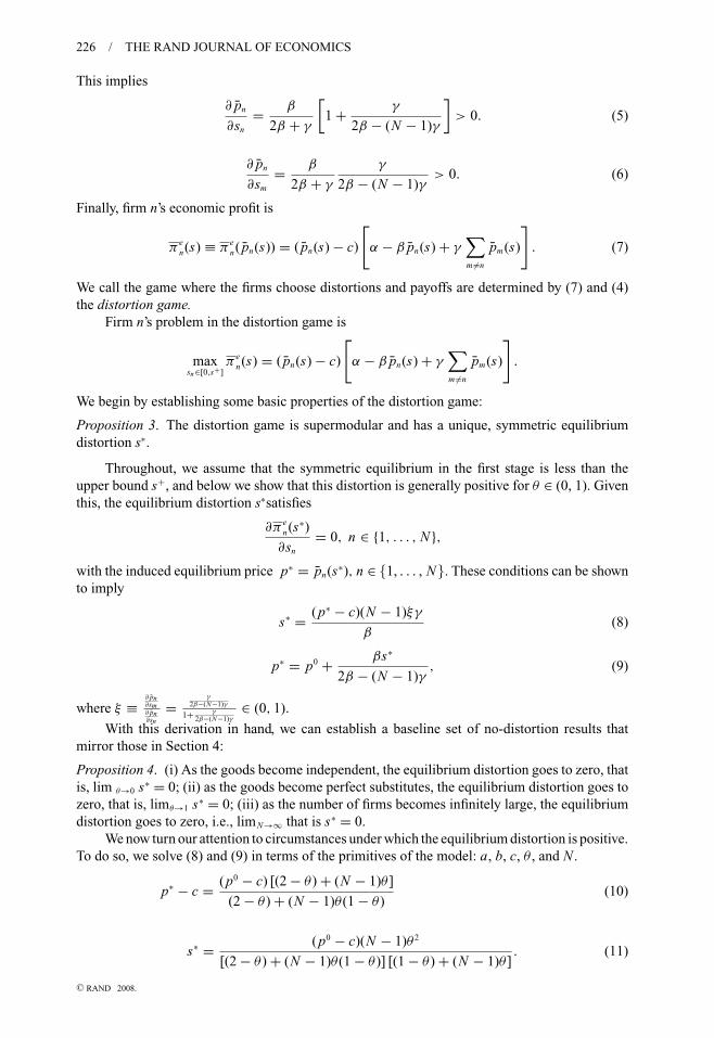
This implies

∂ pn

∂sn

= β

2β + γ

[1 + γ

2β − (N − 1)γ

]> 0. (5)

∂ pn

∂sm

= β

2β + γ

γ

2β − (N − 1)γ> 0. (6)

Finally, firm n’s economic profit is

π en(s) ≡ π e

n( pn(s)) = ( pn(s) − c)

[α − β pn(s) + γ

∑m �=n

pm(s)

]. (7)

We call the game where the firms choose distortions and payoffs are determined by (7) and (4)the distortion game.

Firm n’s problem in the distortion game is

maxsn∈[0,s+]

π en(s) = ( pn(s) − c)

[α − β pn(s) + γ

∑m �=n

pm(s)

].

We begin by establishing some basic properties of the distortion game:

Proposition 3. The distortion game is supermodular and has a unique, symmetric equilibriumdistortion s∗.

Throughout, we assume that the symmetric equilibrium in the first stage is less than theupper bound s+, and below we show that this distortion is generally positive for θ ∈ (0, 1). Giventhis, the equilibrium distortion s∗satisfies

∂π en(s∗)

∂sn

= 0, n ∈ {1, . . . , N },

with the induced equilibrium price p∗ = pn(s∗), n ∈ {1, . . . , N}. These conditions can be shownto imply

s∗ = (p∗ − c)(N − 1)ξγ

β(8)

p∗ = p0 + βs∗

2β − (N − 1)γ, (9)

where ξ ≡∂ pn∂sm∂ pn∂sn

=γ

2β−(N−1)γ

1+ γ2β−(N−1)γ

∈ (0, 1).

With this derivation in hand, we can establish a baseline set of no-distortion results thatmirror those in Section 4:

Proposition 4. (i) As the goods become independent, the equilibrium distortion goes to zero, thatis, lim θ→0 s∗ = 0; (ii) as the goods become perfect substitutes, the equilibrium distortion goes tozero, that is, limθ→1 s∗ = 0; (iii) as the number of firms becomes infinitely large, the equilibriumdistortion goes to zero, i.e., limN→∞ that is s∗ = 0.

We now turn our attention to circumstances under which the equilibrium distortion is positive.To do so, we solve (8) and (9) in terms of the primitives of the model: a, b, c, θ , and N .

p∗ − c = (p0 − c) [(2 − θ ) + (N − 1)θ ]

(2 − θ ) + (N − 1)θ (1 − θ )(10)

s∗ = (p0 − c)(N − 1)θ 2

[(2 − θ ) + (N − 1)θ (1 − θ )] [(1 − θ ) + (N − 1)θ ]. (11)

C© RAND 2008.


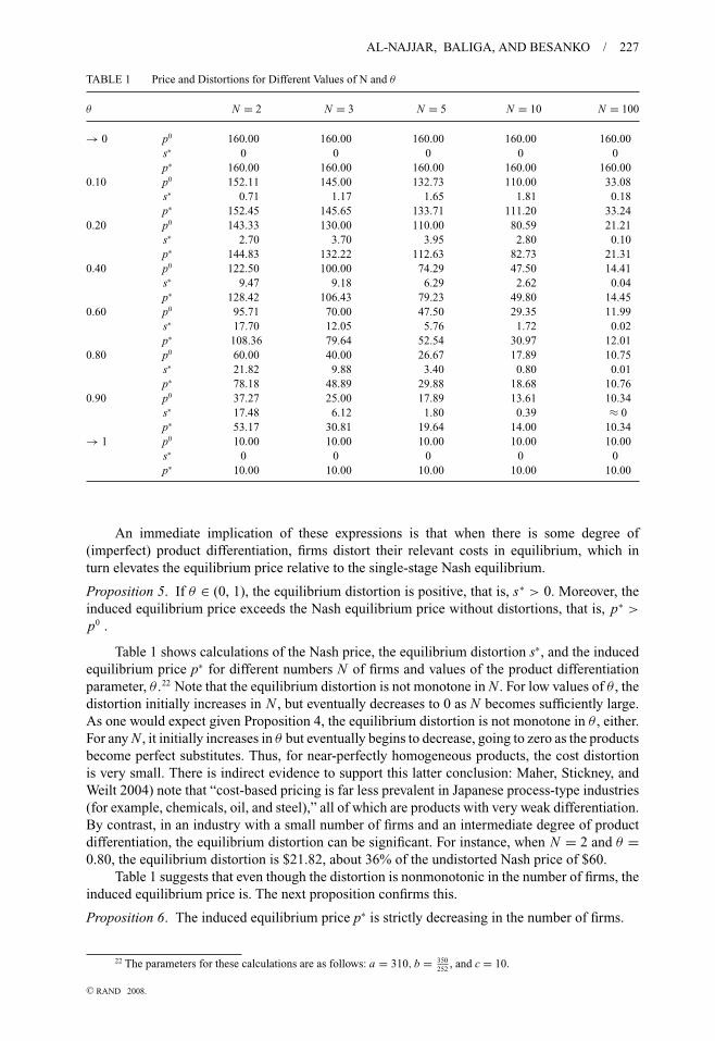
TABLE 1 Price and Distortions for Different Values of N and θ

θ N = 2 N = 3 N = 5 N = 10 N = 100

→ 0 p0 160.00 160.00 160.00 160.00 160.00s∗ 0 0 0 0 0p∗ 160.00 160.00 160.00 160.00 160.00

0.10 p0 152.11 145.00 132.73 110.00 33.08s∗ 0.71 1.17 1.65 1.81 0.18p∗ 152.45 145.65 133.71 111.20 33.24

0.20 p0 143.33 130.00 110.00 80.59 21.21s∗ 2.70 3.70 3.95 2.80 0.10p∗ 144.83 132.22 112.63 82.73 21.31

0.40 p0 122.50 100.00 74.29 47.50 14.41s∗ 9.47 9.18 6.29 2.62 0.04p∗ 128.42 106.43 79.23 49.80 14.45

0.60 p0 95.71 70.00 47.50 29.35 11.99s∗ 17.70 12.05 5.76 1.72 0.02p∗ 108.36 79.64 52.54 30.97 12.01

0.80 p0 60.00 40.00 26.67 17.89 10.75s∗ 21.82 9.88 3.40 0.80 0.01p∗ 78.18 48.89 29.88 18.68 10.76

0.90 p0 37.27 25.00 17.89 13.61 10.34s∗ 17.48 6.12 1.80 0.39 ≈ 0p∗ 53.17 30.81 19.64 14.00 10.34

→ 1 p0 10.00 10.00 10.00 10.00 10.00s∗ 0 0 0 0 0p∗ 10.00 10.00 10.00 10.00 10.00

An immediate implication of these expressions is that when there is some degree of(imperfect) product differentiation, firms distort their relevant costs in equilibrium, which inturn elevates the equilibrium price relative to the single-stage Nash equilibrium.

Proposition 5. If θ ∈ (0, 1), the equilibrium distortion is positive, that is, s∗ > 0. Moreover, theinduced equilibrium price exceeds the Nash equilibrium price without distortions, that is, p∗ >

p0 .

Table 1 shows calculations of the Nash price, the equilibrium distortion s∗, and the inducedequilibrium price p∗ for different numbers N of firms and values of the product differentiationparameter, θ .22 Note that the equilibrium distortion is not monotone in N . For low values of θ , thedistortion initially increases in N , but eventually decreases to 0 as N becomes sufficiently large.As one would expect given Proposition 4, the equilibrium distortion is not monotone in θ , either.For any N , it initially increases in θ but eventually begins to decrease, going to zero as the productsbecome perfect substitutes. Thus, for near-perfectly homogeneous products, the cost distortionis very small. There is indirect evidence to support this latter conclusion: Maher, Stickney, andWeilt 2004) note that “cost-based pricing is far less prevalent in Japanese process-type industries(for example, chemicals, oil, and steel),” all of which are products with very weak differentiation.By contrast, in an industry with a small number of firms and an intermediate degree of productdifferentiation, the equilibrium distortion can be significant. For instance, when N = 2 and θ =0.80, the equilibrium distortion is $21.82, about 36% of the undistorted Nash price of $60.

Table 1 suggests that even though the distortion is nonmonotonic in the number of firms, theinduced equilibrium price is. The next proposition confirms this.

Proposition 6. The induced equilibrium price p∗ is strictly decreasing in the number of firms.

22 The parameters for these calculations are as follows: a = 310, b = 350252

, and c = 10.

C© RAND 2008.


Because firms do not internalize the beneficial impact of their distortion of relevant costs ontheir rivals’ profits, they end up with a price lower than the monopoly price.

Proposition 7. When θ ∈ (0, 1), the induced equilibrium price is less than the monopoly price.

Let us now turn to a comparative statics analysis of the equilibrium distortions with respectto the other parameters of the model, a and c. To avoid conflating the impact of a and c on thedistortion with their effect on the overall price level, we derive the comparative statics result forthe percentage distortion above the undistorted Nash equilibrium price, s∗

p0 .

Proposition 8. The percentage distortion s∗p0 is increasing in a and decreasing in c. Hence an

increase in demand, as measured by a larger value of a, will result in a greater percentagedistortion, whereas an increase in marginal cost will result in a lower-percentage distortion.

This result makes sense. The difference a − c measures the intrinsic value of the industryprofit opportunity. The incremental benefit to a firm from suppressing price competition will begreater the more intrinsically profitable the market is, and, as a result, the degree of distortion isgreater the greater is a or the lower is c.

As a final point, consider the implications of this analysis for entry. Because distortionsincrease equilibrium margins, one would expect that entry would be more desirable in that case,and more firms would come into the industry. We can confirm this intuition. Imagine that eachfirm faces a sunk cost of entry F, and let N 0 and N∗ be the equilibrium number of firms in theno-distortion and distortion cases, respectively. Given the equilibrium number of firms, economicprofit is zero, which implies (

a − p0

b

) (p0 − c

)1 + (N 0 − 1)θ

= F (12)

(a − p∗

b

)(p∗ − c)

1 + (N ∗ − 1)θ= F . (13)

It is straightforward to verify that N ∗ > N 0.

6. Discussion

� Experimental results. As noted in the Introduction, there is strong evidence from thepsychology literature that individual decision makers commit the sunk cost fallacy. A well-citedexample is a study by Arkes and Blumer (1991) which found that the sunk costs incurred byseason ticket holders for a university theater company apparently influenced attendance decisions.

Experimental economists have also studied sunk cost biases, but the evidence from thiswork is more mixed. Economists’ experiments on the sunk cost fallacy differ from those inthe psychology literature in that the latter typically do not focus on decision making in marketsettings in which competition might be expected to create strong pressures for decision makersto “get it right.” By contrast, economists’ experiments on sunk costs generally place subjects inthe context of some sort of market rivalry. For example, Phillip, Battalio & Kogut (1991) studybidding in first-price sealed bid auctions in which subjects paid a sunk admissions fee in orderto participate. They found that 95% of the subjects correctly ignored sunk costs in their biddingbehavior. Summarizing a variety of experiments in competitive market settings in which sunkcosts might effect market outcomes, Smith (2000) writes: “These results showed no evidence ofmarket failure due to the sunk cost fallacy.”

The finding that subjects in competitive market experiments do not succumb to the sunkcost fallacy is consistent with the prediction of our theory that it would run counter to the self-interest of a price-taking firm, or a price-setting firm in a homogeneous product oligopoly, tobase decisions on sunk costs. However, a more direct test of the implications of our theory wouldbe to explore pricing behavior in a differentiated product oligopoly market in which firms incur

C© RAND 2008.


sunk costs. Unfortunately, most of the existing experimental investigations of price competitionin a differentiated product oligopoly (e.g., Dolbear et al., 1968) are not relevant to our theory.This is because these experiments typically provided subjects with a table showing profit as afunction of own price and the prices of rivals. Participants were simply asked to choose a price,and they did not have to figure out for themselves which costs might be relevant for pricingdecisions.

An important exception to this approach is a recent paper by Offerman and Potters (2006).In this study, subjects assumed the role of decision makers in a differentiated product duopoly,and they were given information on firms’ demand curves and marginal costs. Subjects wereplaced in one of three treatments: one in which rights to operate in the market were auctioned tothe two highest bidders; one in which entry rights were allocated randomly to two subjectswho were required to pay an upfront fee23; and one in which entry rights were allocatedrandomly without payment of a fee. Offerman and Potters find that when an entry fee ischarged (either via a fixed fee or by means of an auction), prices are significantly higher thanthe undistorted (symmetric) Nash equilibrium price, but when no entry fee is charged, priceswere close to the undistorted equilibrium price. By contrast, in a monopoly market, prices tendto equal the profit-maximizing monopoly price, irrespective of the level or form of the sunkentry fee.

Our theoretical model gives exactly the same predictions. Our theory implies that amonopolist would have no incentive to succumb to the sunk cost fallacy. In a duopoly withdifferentiated products but with no sunk costs, firms might ultimately benefit from distortingtheir relevant costs, but because they lack a compelling justification for distortionary behavior,our theory would predict that they would end up charging the undistorted Nash equilibriumprice. When sunk costs are present, firms have the opportunity to distort relevant costs upward,and given the demand curves and marginal costs in the Offerman and Potters environment, itmakes sense to do so. Indeed, in this case, the fit between our model and Offerman and Potters’quantitative results is remarkably tight. In the calculations in Table 1 in the previous section,we chose parameters so that when θ = 0.80 and N = 2, we have an economic environmentthat is identical to that in Offerman and Potters’s duopoly experiments.24 As shown in Table 1,the equilibrium price in the two-stage game predicted by our model is 78.18, about 30% higherthan the undistorted Nash equilibrium price of 60. In Offerman and Potters’s fixed entry fee andauction treatments, the average prices were 75.65 and 72.73, respectively.25

Offerman and Potters interpret their results as suggesting that entry fees generate tacitcollusion. In fact, their explanation itself relies on a bounded rationality assumption as theystudy finite repetitions of an oligopoly game which has a unique subgame perfect equilibrium.Moreover, their explanation predicts that tacit collusion should also occur in a Bertrand oligopolywith homogeneous products. This does not coincide with our predictions and hence provides away of testing our theory against theirs.

In conclusion, we note that Offerman and Potters’s experiment is not a formal test of ourmodel. Our model requires separate pricing and costing decisions and a specific timing structurein which adjustments in these decisions occur at different rates. Nevertheless, models shouldideally provide robust insights that hold beyond the narrow formalism on which they are based.It is in this sense that we view their results as suggestive of the plausibility of the core intuitionof our article.

23 Unbeknownst to the subjects, the fixed entry fees were set equal to the entry fees generated in the auctiontreatment.

24 If we set a = 310, b = 350252

, and c = 10, then when θ = 0.80 and N = 2, the firms’ demand curves are

D1(p1, p2) = 124 − 2p1 + 1.6p2 and D2(p1, p2) = 124 − 2p2 + 1.6p1,

exactly as in the Offerman and Potters experiment.25 These calculations are based on the data reported in Table 1 in Offerman and Potters.

C© RAND 2008.


� Cournot competition and behavioral biases. The results for Bertrand competition withproduct differentiation do not transfer to Cournot competition. In contrast to the Bertrand model,firms in the Cournot quantity competition model benefit from becoming more aggressive byproducing higher quantities. To develop intuition, assume there are just two firms and firm 1reduces its output as it suffers from a sunk cost bias. Learning will take place via quantityadjustments, so firm 2 will eventually increase its output and firm 1’s economic profit will godown. Thus, in contrast to a price-setting industry, the sunk cost bias is not reinforced in thecost adjustments phase and our model suggests that the sunk cost bias should disappear in aCournot setting. This provides another refutable implication of our theory that can be tested usingexperimental or field evidence.

In fact, our model suggests that managers may reinforce a bias to overlook relevant costs ina Cournot setting. In an experimental study, Phillip, Battalio, and Kogut (1991) found evidencethat subjects treat opportunity costs as different from direct monetary outlays. In practice, amanager whose firm has purchased an input under a long-term contract may treat the cost ofthat input as sunk when, in fact, it is variable if the input can be resold in the marketplace. Asimilar bias can arise if the contract price of the input is less than the current market price,and the manager computes marginal cost based on the historical, rather than current, marketprice.

� Alternative explanations: noisy observation of cost, delegation, and evolution. Cost andprice distortions may arise as a result of firms observing their total cost but not its split betweenfixed, sunk, and variable components. In this case, rational firms’ estimates of relevant costs arelikely to include non-zero errors similar to the distortions introduced in this article. In this case,a plausible scenario is that firms’ errors have zero mean, in which case no systematic distortionin relevant costs, prices, or profits would appear.

It also is instructive to compare our model with models of strategic delegation (Fershtmanand Judd, 1987) and strategic commitments in general. Strategic commitments matter only tothe extent that they are observable and irreversible. By contrast, firms’ internal accountingmethodologies and their confusions about relevant costs are neither observable nor irreversible.Firms in our model have myopic incentives and arrive at their decisions through a process of naivelearning. They do not actively fine-tune their incentive schemes in anticipation of more favorablesecond-stage equilibrium outcomes. Our model has testable implications that separates it fromthe delegation framework. First, the delegation model would predict higher prices regardless ofthe presence of sunk cost, a prediction that can be experimentally tested. Second, the logic ofdelegation has no bite when prices are set by the firms’ owners, as in experiments where eachfirm is a single subject (so there is literally no delegation). In our model, whether the owner ofthe firm is the same as the agent setting prices is irrelevant.

Related ideas appear in the literature on the evolution of preferences. Samuelson (2001)offers an excellent overview of this literature.26 Closer to our model is the recent workof Heifetz, Shannon, and Spiegel (2004). They offer an interesting model of the evolutionof optimism, pessimism, and interdependent preferences in dominance-solvable games. Likestrategic delegation, the evolution of preferences literature underscores the value of commitment,but this time using distortions of players’ perceptions of their payoffs as a commitment device.The unobservability of firms’ costing practices again separates our model from the evolution ofpreferences approach. For instance, as Dekel, Ely, and Yilankaya (2007) point out, this approachhas little bite when players cannot observe their opponents’ preferences. And as in the delegationparadigm, sunk cost plays no role in evolutionary arguments; these arguments work equally wellin settings where no sunk cost is present.

26 The special issue of the Journal of Economics Theory, 2001, vol. 97 is devoted to this line of research.

C© RAND 2008.


7. Concluding remarks

� There is extensive evidence that real-world decision makers violate the predictions ofstandard economic theory. Among these violations, the sunk bias in pricing decisions standsout on a number of grounds. First, its impact is not limited to small-stakes decisions: pricing isone of the most critical decisions a company can make. Second, unlike other cognitive biasesthat disappear once the underlying fallacy is explained, distorted pricing seems to thrive despitethe relentless efforts of economics and business educators to stamp it out. Third, although manycognitive biases disappear through learning and training, the survey evidence we report providesno indication that this bias is disappearing over time.

In this article, we provided a theory of why confusion of relevant and irrelevant costs persistsin pricing practice.27 We showed that under conditions rooted in actual cost accounting practices,price competition with product differentiation reinforces managers’ innate predisposition toconfound relevant and irrelevant costs. And although there is no reason to suspect thispredisposition to systematically vary across industries, no similar forces appear in monopoly,perfect competition, or price competition in a homogeneous product oligopoly. Thus, our analysismakes predictions that can be empirically and experimentally tested.

Our theory builds on recent advances in learning in games played by naive players whoknow little about their environments. As such, this article illustrates how learning theory can bea valuable tool in understanding the nature of behavioral biases in economics.

Appendix

� The proof of Theorem 1 relies on Proposition 1 and the following result.

Proposition 9. There exists � > 0 such that for any firm n, any vector of distortions s−n ≥ 0, any sn ≤ �, and anyequilibrium price vector p of �(s−n , 0) with corresponding quantity vector q > >0, if p+ is an equilibrium of �(s−n , sn)with p+ > p,

π en (p+) > π e

n (p).

Proof of Theorem 1. Let � be as in Proposition 9 and choose any 0 < sn ≤ �. Fix any s−n and p as in the statementof the theorem. By Proposition 1, any adaptive price adjustment {pt} starting from p for �(s−n, sn) converges top = inf{z ∈ E(s−n, sn), z ≥ p}. It is easy to see that in fact p >> p. The result now follows from Proposition 9.

Proof of Proposition 9. Suppose, by way of contradiction, that for every positive integer k, there is sn < 1/k, a vector ofdistortions sk

−n , an equilibrium pk of �(sk−n, 0), and an equilibrium pk of �(sk

−n , sn) with pk > pk yet π en ( pk) ≤ π e

n ( pk).Passing to subsequences if necessary, we may assume that sk

−n → s−n, pk → p, and pk → p. Clearly, p ≥ p and π en ( p) ≤

π en ( p). We note that, by Lemma 2 below, p is an equilibrium of �(s−n , 0). We consider two cases.

Case 1. p > p. In this case, the fact that best responses are strictly increasing implies p >> p. Next we show thatπ e

n ( p) > π en ( p). From our assumptions on demand and the fact that q > >0.

πn( p−n, pn, sn = 0) > πn( p, sn = 0) = π en ( p). (A1)

That is, relative to p, firm n achieves higher profit if its opponents strictly increase their prices while all other pricesremain unchanged. Because p is an equilibrium, we must also have

π en ( p) = πn( p, sn = 0) ≥ πn( p−n, pn, sn = 0),

which combining with (A1) implies π en ( p) > π e

n ( p). By the continuity of π en , for k large enough, π e

n ( pk ) > π en ( pk ), a

contradiction.

27 The only other model we are aware of that studies the effect of the sunk cost bias in differentiated Bertrandcompetition is by Parayre (1995). He considers a two-stage game in a linear environment similar to the special case ofsymmetric linear demand we study in Section 5 (in his model, no naive learning justification of behavior is considered).Parayre assumes that the sunk cost bias has the implication that firms produce in order to use up whatever capacity isavailable to them. Compared to the standard Bertrand equilibrium, Parayre’s model leads to lower prices and profits. Ourmodel sheds light on the form of distortion that is likely to persist in a competitive environment. Although the formof distortion we propose will be perpetuated in the long run, our model predicts that Parayre’s form of distortion mustdisappear.

C© RAND 2008.


Case 2. p = p. For each k, define

zk = pk − pk

‖pk − pk‖ .

Let SN denote the unit sphere and, given α > 0, define B α = SN ∩ {x N ∈ RN+ , x n ≤ 1 − α}. We first need the following

lemma.

Lemma 1. There is α > 0 such that for all large-enough k, zk ∈ B α .

From the definition of derivatives, for every ε > 0, there is h such that for any 0 < h < h and any z ∈ SN ,∣∣∣∣π en ( pk + hz) − π e

n ( pk)

h− [∂π e

n ( pk)]z

∣∣∣∣ < ε,

where ∂π en ( pk) is a row vector of partial derivatives of π e

n evaluated at pk . Notice that ∂πen

∂ pn( pk ) = 0 as pk is an equilibrium

and ∂πen

∂ pm( pk ) > 0 as ∂Dn

∂ pm> 0 for m �= n and qk

m > 0 for all k large enough. Note that [∂π en ( p)]z > 0 for all z ∈ B α .

Next we note that

lim infk→∞

minz∈Bα

pk ∈(sk−n ,0)

[∂π e

n ( pk)]z ≥ min

z∈Bαp∈(s−n ,0)

[∂π e

n ( p)]z.

To see this, write

minz∈Bα

pk ∈(sk−n ,0)

[∂π e

n ( pk)]z =

[∂π e

n ( pk)]zk .28

For any pair of subsequences { pl}, {zl} converging to p and z, respectively, we have z ∈ Bα and p ∈ (s−n, 0) (the latterholds by Lemma 2). From the continuity of π e

n we have

minz∈Bα

pl ∈(sl−n ,0)

[∂π e

n ( pl )]z =

[∂π e

n ( pl )]z →

[∂π e

n ( p)]z ≥ min

z∈Bαp∈(s−n ,0)

[∂π e

n ( p)]z.

Fix α > 0 and set ε = 0.25 min z∈Bαp∈(s−n ,0)

[∂π en ( p)]z. Then, given any z ∈ B α and pk ∈ (sk

−n, 0), for all k large enoughwe have

π en ( pk ) − π e

n ( pk)

‖ pk − pk ‖ ≡ π en ( pk + ‖ pk − pk ‖zk ) − π e

n ( pk)

‖ pk − pk ‖>

[∂π e

n ( pk )]zk − ε

≥ min z∈Bα

pk ∈(sk−n ,0)

[∂π e

n ( pk)]z − ε

≥ 0.5 min z∈Bαp∈(s−n ,0)

[∂π e

n ( p)]z − ε

≥ 0.25 min z∈Bαp∈(s−n ,0)

[∂π e

n ( p)]z > 0.

Hence π en ( pk) − π e

n ( pk) > 0 for all k large enough. A contradiction.

Proof of Lemma 2. Given k, for m �= n

limh→0

rm( p−n, pn + h, sm) − pm

h= ∂rm

∂ pn

( p, sm).

As pk → p, pk → p, and sk−n → s−n, because ∂rm

∂ pnis continuous, for every ε > 0, there is a k such that for all k > k

rm

(pk

−n, pkn + (

pkn − pk

n

), sk

m

)− pk

m(pk

n − pkn

) >∂rm

∂pn

( p, sm) − ε (A2)

for all m �= n.Note further that

pkm = rm

(pk

−n, pkn, sk

m

)= rm

(pk

−n, pkn +

(pk

n − pkn

), sk

m

)and hence from (A2), for every ε > 0, for all k large enough and all m �= n,

pkm − pk

m

pkn − pk

n

>∂rm

∂ pn

( p, sm) − ε > 0

if ε is small enough.

28 The minimum is achieved by the compactness of B α and (sk −n , 0).

C© RAND 2008.


To prove the lemma, suppose, by way of contradiction, that {zk} has as an accumulation point the unit vector z withz

′n = 1 and all other entries equal to zero. Passing to subsequences if necessary, we may assume that zk → z′. This implies

that pkm − pk

m

|| pk − pk || → 0 for every m �= n, and pkn − pk

n

|| pk − pk || → 1. Thus, given any τ > 0, for ε small and for all k large enough,

| pkn − pk

n

|| pk − pk || − 1| < τ , hence || pk − pk || <pk

n − pkn

1−τ. Then for m �= n,

‖ zk − z′ ‖ ≥ pkm − pk

m

‖ pk − pk‖ ≥ pkm − pk

m

pkn − pn

1 − τ

> (1 − τ )

(∂rm

∂ pn

( p, sm) − ε

)> 0,

contradicting the assumption that zk → z′.Lemma 2. Suppose that sk → s, and pk → p where for each k, pk is an equilibrium of �(sk). Then p is an equilibriumof �(s).

Proof . If p were not an equilibrium of �(s), then there would be a firm m and a strategy p′m such that

πm(p−m, p′m , sm) > πm(p−m , pm , sm).

Because π m is continuous in p and s m , for all-large enough k,

πm

(pk

−m , p′m , sk

m

)> πm

(pk

−m , pkm , sk

m

).

This contradicts the fact that pk is an equilibrium of �(sk ) for all k.Lemma 3. For any s−n , s n ≥ �, and p ∈ E(s),

p0 ≡ sup{z ∈ E(s−n, 0), z ≤ p} << inf{z ∈ E(s−n, �), z ≥ p0} ≤ sup{z ∈ E(s−n,�), z ≤ p}.

Proof . First, note that, because best responses are strictly increasing in opponents’ prices and cost, p0 << p. Define asequence of price vectors {pt}∞

t=0 such that p0 = sup{z ∈ E(s−n, 0), z ≤ p}, and for t > 0,

pt = (rm(pt−1, sm), m �= n, rn(pt−1,�)).

We show by induction that pt << p for all t. The claim holds by definition for t = 0. Assume that it holds for t ≥ 0, thenbecause pt,−m << p−m for all m, and best responses are strictly increasing in opponents’ prices, r m(pt , s m) < r m(p, s m).A similar argument shows that pt >>P 0 for all t > 0. Because [p0, p] is compact, passing to subsequences if necessary,we may assume that pt → P� ∈ [P0, P]. Because {pt} is an adaptive pricing adjustment starting at p0, by Proposition 1,p = in f {z ∈ E(s−n, �), z ≥ p0}. Clearly, p� ≤ sup{z ∈ E(s−n, �), z ≤ p}.Lemma 4. There is φ > 0 such that for any s and p ∈ E(s),

n(s−n, �, p) − n(s−n, 0, p) > φ.

Proof . Consider any s ′, p′ ∈ E(s ′). Assume first that sn > �. By Proposition 1,

n(s ′−n, �, p′) − n(s ′

−n, 0, p′) = π en (sup{z ∈ E(s ′

−n, �), z ≤ p′})−π e

n (sup{z ∈ E(s ′−n, 0), z ≤ p′}).

Combining Lemma 3 and Proposition 9, this expression is strictly positive for every s ′, p′ ∈ E(s ′). The conclusion nowfollows from the facts that s ′ ranges over a finite set, E(s ′) is compact for every s ′, and π e

n is continuous. The remainingcases s

′n = 0, � can be dealt with similarly.

Proof of Theorem 2. Choose � as in Proposition 9. Fix an arbitrary firm n and define L τ (s) to be the sum of payoffs inall periods τ ′ < τ such that τ

′was an experimental period and the distortion was chosen. For any 0 < δ < � define

Xτ = Lτ (δ) − Lτ (0).

Because experiments are independent across periods and all distortions are picked with equal probability, the strong lawof large numbers implies that, almost surely, for all τ large enough, all distortions are played with equal frequencies.Thus, for all large nonexperimental periods τ , X τ > 0 implies that firm n does not choose s n = 0. Thus, to prove thetheorem, it suffices to show that X τ → ∞ almost surely.

C© RAND 2008.


Define

xτ = [Lτ (δ) − Lτ (0)] − [Lτ−1(δ) − Lτ−1(0)]

yτ = xτ − E(xτ | hτ−1), zτ = E(xτ | hτ−1)

Yτ =τ∑

s=1

ys, Zτ =τ∑

s=1

zs .

Clearly,

Xτ = Yτ + Zτ ,29 (A3)

and {Y τ} is a martingale.30 Because each Y τ has bounded support, by Theorem 6.8.5 in Ash and Doleans-Dade (2000),the random variables Y τ − Y τ−1 = y τ are orthogonal, and by Theorem 5.1.2 Chung (1974), Yτ

τ=

∑∞s=1 ys

τ, → 0 almost

surely (i.e. the conclusion of the law of large numbers holds). From this and equation (A3), it follows that

Xτ − Zτ

τ→ 0 a.s. (A4)

On the other hand,

zτ = E([Lτ (δ) − Lτ (0)] − [Lτ−1(δ) − Lτ−1(0)] | hτ−1)

= E(n(s−n(τ ), δ, p(τ − 1)) − n(s−n(τ ), 0, p(τ − 1)) | hτ−1)

≥ 1

N

ε

Kφ > 0,

where the last two inequalities follow from Lemma 4, and K is the number of distortions in the grid. This implies thatZτ

τ≥ 1

Nε

Kφ. This fact and equation (A4) imply X τ → ∞ almost surely.

Proof of Proposition 2. In any equilibrium of the pricing game, the lowest price offered must be at or just below thesecond-highest cost including any distortion. Suppose this is not the case and let p∗ be the lowest-price. Then, of thetwo lowest cost firms, at least one is not capturing the entire market. But that firm can price just under p∗ and capturethe entire market and increase its accounting profit, a contradiction. Also, in any equilibrium, the firm with the lowestcost including distortions must be setting the lowest price. Otherwise, it is making zero profits and can deviate and makepositive accounting profit by matching the lowest price. If its cost including distortion is lower than the second-highestcost, it will price slightly below the second-highest cost to capture the entire market. This observation implies that in anyequilibrium with no distortions, the lowest price must be at or just below c2 . Also, firm 1 must be setting the lowest priceand either capturing the entire market, if c2 > c1, or sharing it, if c1 = c2 . In either case, firms 2 and above make zeroprofits and firm 1 makes positive profits only if c2 > c1.

Suppose firm 2 or higher distorts its relevant costs upward by s. Then, let c∗ be the lowest cost including thedistortion among all the firms apart from firm 1. By our argument above, any equilibrium of the pricing game musthave the price set at or just below c∗. Therefore, firms 2 and higher make zero profits in equilibrium and hence have noincentive to distort their relevant costs upward. Now, suppose firm 1 distorts upward by s. If c1 + s < c2, then there is nochange in the equilibrium in the pricing game and hence no incentive to distort. If c1 + s > c2, in any equilibrium in thepricing game, firm 1 must make zero profits as firm 2 has the lowest cost and will always undercut the price set by the firmwith the second-highest cost including any distortion. Hence, firm 1 has no incentive to distort relevant costs upward.Moreover, there is no incentive for firm 1 to distort downward as it does not alter the pricing equilibrium. Similarly, iffirm n > 1 distorts downward by s it still makes zero profits, when cn − s ≥ c1, or makes a loss, when cn − s < c1, andit sets a price just under c1 which is less than its true cost cn . �Proof of Proposition 3. We establish existence by showing that π e

n (s) is supermodular in s (Milgrom and Roberts, 1990).Differentiating π e

n(s) with respect to s n we have

∂π en(s)

∂sn

=[−β ( pn(s) − c) + α − β pn(s) + γ

∑m �=n

pm(s)

]∂ pn

∂sn

+ ( pn(s) − c) γ∑m �=n

∂ pm

∂sn

.

Using (3), we can write this as

∂π en(s)

∂sn

= −β∂ pn

∂sn

sn + (N − 1)γ∂ pm

∂sn

( pn(s) − c) , (A5)

where ∂ pn

∂snand ∂ pn

∂smare given by (5) and (6), respectively. This implies

∂2π en (s)

∂sn∂sm

= (N − 1)γ

(∂ pn

∂sm

) (∂ pm

∂sn

)> 0.

29 This is the well-known Doob decomposition. See, for instance, Chung, (1974).30 E(Y τ+1 | Y τ ) = E(y τ+1 + Y τ | Y τ ) = E(x τ+1 | Y τ ) − E(E(x τ+1 | Y τ ) | Y τ ) + Y τ = Y τ .

C© RAND 2008.


Thus, the first-stage game is supermodular in s. To establish uniqueness we establish the contraction condition � ≡∂2 πe

n (s)∂s2

n+ ∑

n �=m∂2 πe

n (s)∂sn ∂sm

< 0 for all s ≥ 0. We first note that

∂2π en (s)

∂s2n

= ∂ pn

∂sn

[−β + (N − 1)γ

∂ pm

∂sn

].

Thus, we can write

� = ∂ pn

∂sn

{−β + [

(N − 1)γ + (N − 1)2γ ξ] ∂ pm

∂sn

},

where ξ ≡∂ pn∂sm∂ pn∂sn

=γ

2β−(N−1)γ

1+ γ2β−(N−1)γ

∈ (0, 1). because ∂ pn

∂sn> 0 and ∂ pm

∂sn= β

2β+γ

γ

2β−(N−1)γ,� < 0 if and only if

[(N − 1) + (N − 1)2ξ ]γ 2

(2β + γ ) (2β − (N − 1)γ )< 1. (A6)

Now, straightforward algebra establishes that

γ 2

(2β + γ ) (2β − (N − 1)γ )=

(θ

(N − 1)θ + 2(1 − θ )

) (θ

(2N − 1)θ + 2(1 − θ )

).

Furthermore ξ < 1, so (N − 1) + (N − 1)2 ξ < (N − 1) + (N − 1)2 = N (N − 1). Thus

[(N − 1) + (N − 1)2ξ ]γ 2

(2β + γ ) (2β − (N − 1)γ )

<

((N − 1)θ

(N − 1)θ + 2(1 − θ )

)(Nθ

(2N − 1)θ + 2(1 − θ )

).

But N < 2N − 1, because N > 1. Thus((N − 1)θ

(N − 1)θ + 2(1 − θ )

)(Nθ

(2N − 1)θ + 2(1 − θ )

)

<

((N − 1)θ

(N − 1)θ + 2(1 − θ )

)((2N − 1) θ

(2N − 1)θ + 2(1 − θ )

).

Because each term in the above expression is positive but less than one, we immediately have((N − 1)θ

(N − 1)θ + 2(1 − θ )

)((2N − 1) θ

(2N − 1)θ + 2(1 − θ )

)< 1,

which establishes that � < 0. The equilibrium in sn is thus unique, and because firms are symmetric, the equilibriumdistortion will be symmetric across firms.

Proof of Proposition 4.

Proof (i). We begin by noting that θ = 0 ⇒ γ = 0 and β = 1b. Using this, it is straightforward to verify that limθ→0

∂πen

∂sn=

− sn

2b< 0. Hence, no firm has an incentive to choose a positive distortion.

Proof (ii). It is straightforward to show that

limθ→1

p0 = c

limθ→1

γ

β= 1

N − 1

limθ→1

β

2β − (N − 1)γ= 1

limθ→1

ξ = 1

N.

Now let s∗ (1) = lim θ→ 1 s∗ and p∗ (1) = lim θ→ 1 p∗ . Taking limits of each side of (8) and (9), and using the expressionsabove, we have

s∗(1) = (p∗(1) − c)

Np∗(1) = c + s∗(1).

These can only be satisfied if s∗ (1) = 0 and p∗ (1) = c.

C© RAND 2008.


Proof (iii). It is straightforward to show that

limN→∞

p0 = c

limN→∞

(N − 1)ξ = 1

limN→∞

γ

β= 0.

Now let s∗ (∞) = lim N→∞ s∗ and p∗ (∞) = lim N→∞ p∗. Taking limits of (8) and using the above expressions impliesthat s∗ (∞) = 0.

Proof of Proposition 5. If θ ∈ (0, 1), then p0 > c. Furthermore, it is straightforward to show that

(N − 1)θ 2

[(2 − θ ) + (N − 1)θ (1 − θ )] [(1 − θ ) + (N − 1)θ ]> 0,

which implies that s∗ > 0. When θ ∈ (0, 1),

(2 − θ ) + (N − 1)θ

(2 − θ ) + (N − 1)θ (1 − θ )> 1.

Thus, p∗ − c > p0 − c, or p∗ > p0 .

Proof of Proposition 6. The expression for p∗ − c can be written as follows:

p∗ − c = (a − c)(1 − θ )y(N )z(N ),

where

y(N ) = 1

2 − θ + (N − 1)θ (1 − θ )

z(N ) = 2 − θ + (N − 1)θ

2(1 − θ ) + (N − 1)θ.

Clearly y(N) is strictly decreasing in N and so too is z(N):

z′(N ) = − θ 2

[2(1 − θ ) + (N − 1)θ ]2 < 0.

Hence p∗ − c is strictly decreasing in N .

Proof of Proposition 7. The monopoly price pM satisfies

pM − c = a − c

2.

From (10), p∗ − c can be written as

p∗ − c = (a − c)(1 − θ ) [2 − θ + (N − 1)θ )]

[2 − θ + (N − 1)θ (1 − θ )] [2(1 − θ ) + (N − 1)θ ].

p∗ < pM if and only if

(1 − θ ) [2 − θ + (N − 1)θ ]

[2 − θ + (N − 1)θ (1 − θ )] [2(1 − θ ) + (N − 1)θ ]<

1

2. (A7)

This can be rewritten as

[2 − θ + (N − 1)θ (1 − θ )] [2(1 − θ ) + (N − 1)θ ] > 2(1 − θ ) [2 − θ + (N − 1)θ ] .

Now, for N ≥ 3, [2(1 − θ ) + (N − 1)θ ] ≥ 2 because θ ∈ (0, 1) and N − 1 ≥ 2. Hence, we have

[2 − θ + (N − 1)θ (1 − θ )] [2(1 − θ ) + (N − 1)θ ] > 2 [2 − θ + (N − 1)θ (1 − θ )]

> 2(1 − θ )[2 − θ + (N − 1)θ ].

For N = 2, the inequality (A7) boils down to

1 − θ

2 − θ<

2 − θ 2

4,

which can be shown to hold for θ ∈ (0, 1). Hence, (A7) holds for all N ≥ 2, establishing p∗ < pM .

Proof of Proposition 8. These results follow directly from expression (11).

C© RAND 2008.


References

ALCHIAN, A. “Uncertainty, Evolution, and Economic Theory.” Journal of Political Economy, Vol. 58 (1950), pp. 211–221.ARKES, H.R. AND AYTON, P. “The Sunk Cost and Concorde Effects: Are Humans Less Rational Than Lower Animals?”

Psychological Bulletin, Vol. 125 (1999), pp. 591–600.—— AND BLUMER, C. “The Psychology of Sunk Cost.” Organizational Behavior and Human Decision Processes, Vol.

35 (1991), pp. 124–140.ASH, R. AND DOLEANS-DADE, C. Probability and Measure Theory, 2d ed. New York: Harcourt/Academic Press, 2000.BROWN, D., BOOTH, P., AND GIACOBBE, F. “Technological and Organizational Influences on the Adoption of Activity-Based

Costing in Australia.” Accounting and Finance, Vol. 44 (2004), pp. 329–356.CHUNG, K.L. A Course in Probability Theory, 3d ed. New York: Academic Press, 1974.DEKEL, E., ELY, J.C., AND YILANKAYA, O. “Evolution of Preferences.” Review of Economic Studies,Vol. 74 (2007), pp.

685–704.DOLBEAR, F., LAVE, L., BOWMAN, G., LIEBERMAN, A., PRESCOTT, E., REUTER, F., AND SHERMAN, R. “Collusion in Oligopoly.”

Quarterly Journal of Economics, Vol. 82 (1968), pp. 240–259.ECHENIQUE, F. “Comparative Statics by Adaptive Dynamics and the Correspondence Principle.” Econometrica, Vol. 70

(2002), pp. 833–844.FERSHTMAN, C. AND JUDD, K. “Equilibrium Incentives in Oligopoly.” American Economic Review, Vol. 77 (1987),

pp. 927–940.FINANCIAL ACCOUNTING STANDARDS BOARD. “Qualitative Characteristics of Accounting Information.” Statement of

Financial Accounting Concepts,No. 2, May 1980, http://www.fasb.org/st/.FRIEDMAN, J.W. AND MEZZETTI, C. “Learning in Games by Random Sampling.” Journal of Economic Theory, Vol. 98

(2001), pp. 55–84.GOVINDARAJAN, V. AND ANTHONY, R. “How Firms Use Cost Data in Pricing Decisions.” Management Accounting,

Vol. 76 (1995), pp. 37–39.HART, S. AND MAS-COLELL, A. “A Simple Adaptive Procedure Leading to Correlated Equilibrium.” Econometrica,

Vol. 68 (2000), pp. 1127–1150.HEIFETZ, A., SHANNON, C., AND SPIEGEL, Y. “The Dynamic Evolution of Preferences.”Economic Theory, Vol. 33 (2007)

pp. 251–286.HORNGREN, C., FOSTER, G., AND DATAR, S. Cost Accounting, 9th ed. Upper Saddle River, NJ: Prentice Hall, 2000.KAPLAN, R. AND ATKINSON, A. Advanced Management Accounting, 2d ed. Englewood Cliffs, NJ: Prentice-Hall, 1989.MAHER, M., STICKNEY, C., AND WEIL, R.L. Managerial Accounting, 8th ed. Mason, OH: South-Western, 2004.MILGROM, P. AND ROBERTS, J. “Rationalizability, Learning, and Equilibrium in Games with Strategic Complementarities.”

Econometrica, Vol. 58 (1990), pp. 1255–1277.—— AND ——. “Adaptive and Sophisticated Learning in Normal Form Games.” Games and Economic Behavior, Vol.

3 (1991), pp. 82–100.OFFERMAN, T. AND POTTERS, J. “Does Auctioning of Entry Licenses Induce Collusion? An Experimental Study.” Review

of Economic Studies, Vol. 73 (2006), pp. 769–791.PARAYRE, R. “The Strategic Implications of Sunk Costs: A Behavioral Perspective.” Journal of Economic Behavior and

Organization, Vol. 28 (1995), pp. 417–442.PHILLIP, O., BATTALIO, R., AND KOGUT, C. “Sunk and Opportunity Costs in Valuation and Bidding.” Southern Economic

Journal, Vol. 58 (1991), pp. 112–128.ROZTOCKI, N. AND SCHULTZ, S. “Adoption and Implementation of Activity-Based Costing: A Web-Based Sur-

vey.”Proceedings of the 12th Annual Industrial Engineering Research Conference (IERC 2003), Portland, OR,May 18–20, 2003.

SAMUELSON, L. “Introduction to Evolution of Preferences.” Journal of Economic Theory, Vol. 97 (2001), pp. 225–230.SHANK, J. AND GOVINDARAJAN, V. Strategic Cost Analysis. Burr Ridge, IL: Irwin, 1989.SHIM, E. “Cost Management and Activity-Based Costing in a New Manufacturing Environment.” Unpublished

Dissertation, Rutgers University, 1993.—— AND SUDIT, E. “How Manufacturers Price Products.” Management Accounting, Vol. 76 (1995), pp. 37–39.SMITH, V. “Rational Choice: The Contrast between Economics and Psychology.” In Bargaining in Market Experiments,

ed. V. Smith, Cambridge UK: Cambridge University Press, 2000.THALER, R. “Towards a Positive Theory of Consumer Choice.” Journal of Economic Behavior and Organization, Vol. 1

(1980), pp. 39–60.VIVES, X. Oligopoly Pricing. Cambridge, MA: MIT Press, 1999.

C© RAND 2008.

market forces meet behavioral biases: cost … forces meet behavioral biases: cost misallocation and...

Documents