markov decision processes and dynamic...
TRANSCRIPT

MVA-RL Course
Markov Decision Processes and Dynamic Programming
A. LAZARIC (SequeL Team @INRIA-Lille)ENS Cachan - Master 2 MVA
SequeL – INRIA Lille
How to model an RL problem
The Markov Decision Process
Tools
Model
Value Functions
A. LAZARIC – Markov Decision Process and Dynamic Programming Sept 29th, 2015 - 2/103
How to model an RL problem
The Markov Decision Process
Tools
Model
Value Functions
A. LAZARIC – Markov Decision Process and Dynamic Programming Sept 29th, 2015 - 2/103
Mathematical Tools
How to model an RL problem
The Markov Decision Process
Tools
Model
Value Functions
A. LAZARIC – Markov Decision Process and Dynamic Programming Sept 29th, 2015 - 3/103

Mathematical Tools
Probability Theory
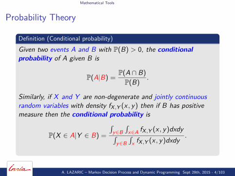
Definition (Conditional probability)Given two events A and B with P(B) > 0, the conditionalprobability of A given B is
P(A|B) =P(A ∩ B)
P(B).
Similarly, if X and Y are non-degenerate and jointly continuousrandom variables with density fX ,Y (x , y) then if B has positivemeasure then the conditional probability is
P(X ∈ A|Y ∈ B) =
∫y∈B
∫x∈A fX ,Y (x , y)dxdy∫
y∈B∫
x fX ,Y (x , y)dxdy.
A. LAZARIC – Markov Decision Process and Dynamic Programming Sept 29th, 2015 - 4/103
Mathematical Tools
Probability Theory
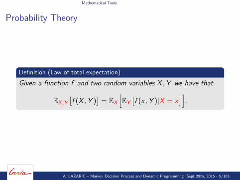
Definition (Law of total expectation)Given a function f and two random variables X ,Y we have that
EX ,Y[f (X ,Y )
]= EX
[EY[f (x ,Y )|X = x
]].
A. LAZARIC – Markov Decision Process and Dynamic Programming Sept 29th, 2015 - 5/103
Mathematical Tools
Norms and Contractions
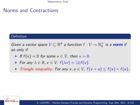
Definition
Given a vector space V ⊆ Rd a function f : V → R+0 is a norm if
an only ifI If f (v) = 0 for some v ∈ V, then v = 0.I For any λ ∈ R, v ∈ V, f (λv) = |λ|f (v).I Triangle inequality: For any v , u ∈ V, f (v + u) ≤ f (v) + f (u).
A. LAZARIC – Markov Decision Process and Dynamic Programming Sept 29th, 2015 - 6/103
Mathematical Tools
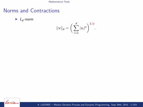
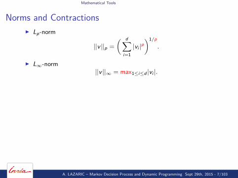
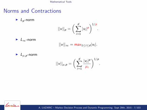
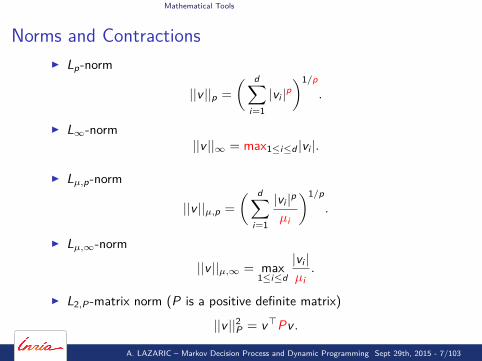
Norms and ContractionsI Lp-norm
||v ||p =
( d∑i=1|vi |p
)1/p.
I L∞-norm||v ||∞ = max1≤i≤d |vi |.
I Lµ,p-norm
||v ||µ,p =
( d∑i=1
|vi |p
µi
)1/p.
I Lµ,∞-norm
||v ||µ,∞ = max1≤i≤d
|vi |µi.
I L2,P -matrix norm (P is a positive definite matrix)
||v ||2P = v>Pv .
A. LAZARIC – Markov Decision Process and Dynamic Programming Sept 29th, 2015 - 7/103
Mathematical Tools
Norms and ContractionsI Lp-norm
||v ||p =
( d∑i=1|vi |p
)1/p.
I L∞-norm||v ||∞ = max1≤i≤d |vi |.
I Lµ,p-norm
||v ||µ,p =
( d∑i=1
|vi |p
µi
)1/p.
I Lµ,∞-norm
||v ||µ,∞ = max1≤i≤d
|vi |µi.
I L2,P -matrix norm (P is a positive definite matrix)
||v ||2P = v>Pv .
A. LAZARIC – Markov Decision Process and Dynamic Programming Sept 29th, 2015 - 7/103
Mathematical Tools
Norms and Contractions
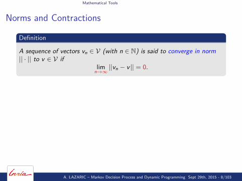
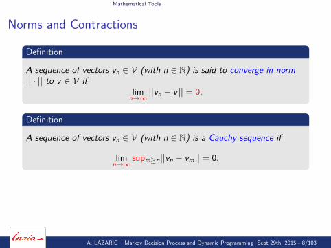
Definition
A sequence of vectors vn ∈ V (with n ∈ N) is said to converge in norm|| · || to v ∈ V if
limn→∞
||vn − v || = 0.
Definition
A sequence of vectors vn ∈ V (with n ∈ N) is a Cauchy sequence if
limn→∞
supm≥n||vn − vm|| = 0.
Definition
A vector space V equipped with a norm || · || is complete if every Cauchysequence in V is convergent in the norm of the space.
A. LAZARIC – Markov Decision Process and Dynamic Programming Sept 29th, 2015 - 8/103
Mathematical Tools
Norms and Contractions
Definition
A sequence of vectors vn ∈ V (with n ∈ N) is said to converge in norm|| · || to v ∈ V if
limn→∞
||vn − v || = 0.
Definition
A sequence of vectors vn ∈ V (with n ∈ N) is a Cauchy sequence if
limn→∞
supm≥n||vn − vm|| = 0.
Definition
A vector space V equipped with a norm || · || is complete if every Cauchysequence in V is convergent in the norm of the space.
A. LAZARIC – Markov Decision Process and Dynamic Programming Sept 29th, 2015 - 8/103
Mathematical Tools
Norms and Contractions
Definition
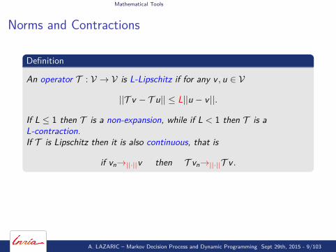
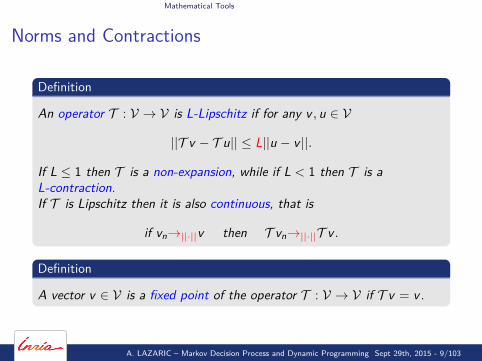
An operator T : V → V is L-Lipschitz if for any v , u ∈ V
||T v − T u|| ≤ L||u − v ||.
If L ≤ 1 then T is a non-expansion, while if L < 1 then T is aL-contraction.If T is Lipschitz then it is also continuous, that is
if vn→||·||v then T vn→||·||T v .
Definition
A vector v ∈ V is a fixed point of the operator T : V → V if T v = v.
A. LAZARIC – Markov Decision Process and Dynamic Programming Sept 29th, 2015 - 9/103
Mathematical Tools
Norms and Contractions
Definition
An operator T : V → V is L-Lipschitz if for any v , u ∈ V
||T v − T u|| ≤ L||u − v ||.
If L ≤ 1 then T is a non-expansion, while if L < 1 then T is aL-contraction.If T is Lipschitz then it is also continuous, that is
if vn→||·||v then T vn→||·||T v .
Definition
A vector v ∈ V is a fixed point of the operator T : V → V if T v = v.
A. LAZARIC – Markov Decision Process and Dynamic Programming Sept 29th, 2015 - 9/103
Mathematical Tools
Norms and Contractions
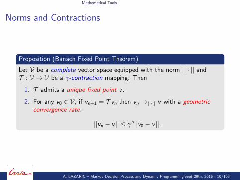
Proposition (Banach Fixed Point Theorem)Let V be a complete vector space equipped with the norm || · || andT : V → V be a γ-contraction mapping. Then
1. T admits a unique fixed point v .
2. For any v0 ∈ V, if vn+1 = T vn then vn →||·|| v with a geometricconvergence rate:
||vn − v || ≤ γn||v0 − v ||.
A. LAZARIC – Markov Decision Process and Dynamic Programming Sept 29th, 2015 - 10/103

Mathematical Tools
Linear Algebra
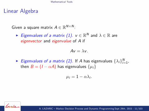
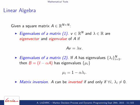
Given a square matrix A ∈ RN×N :I Eigenvalues of a matrix (1). v ∈ RN and λ ∈ R are
eigenvector and eigenvalue of A if
Av = λv .
I Eigenvalues of a matrix (2). If A has eigenvalues {λi}Ni=1,then B = (I − αA) has eigenvalues {µi}
µi = 1− αλi .
I Matrix inversion. A can be inverted if and only if ∀i , λi 6= 0.
A. LAZARIC – Markov Decision Process and Dynamic Programming Sept 29th, 2015 - 11/103
Mathematical Tools
Linear Algebra
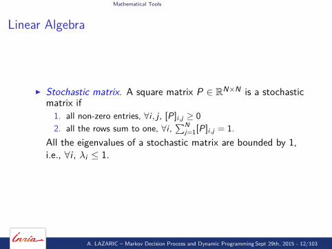
I Stochastic matrix. A square matrix P ∈ RN×N is a stochasticmatrix if
1. all non-zero entries, ∀i , j , [P]i,j ≥ 02. all the rows sum to one, ∀i ,
∑Nj=1[P]i,j = 1.
All the eigenvalues of a stochastic matrix are bounded by 1,i.e., ∀i , λi ≤ 1.
A. LAZARIC – Markov Decision Process and Dynamic Programming Sept 29th, 2015 - 12/103
The Markov Decision Process
How to model an RL problem
The Markov Decision Process
Tools
Model
Value Functions
A. LAZARIC – Markov Decision Process and Dynamic Programming Sept 29th, 2015 - 13/103
The Markov Decision Process
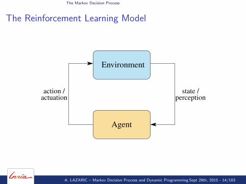
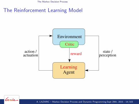
The Reinforcement Learning Model
Environment
Agent
actuationaction / state /
perception
A. LAZARIC – Markov Decision Process and Dynamic Programming Sept 29th, 2015 - 14/103
The Markov Decision Process
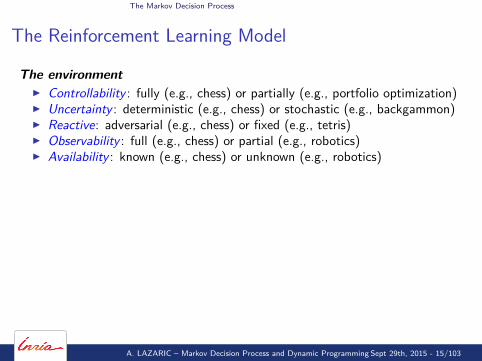
The Reinforcement Learning Model
Environment
AgentLearning
Critic
perceptionactuationaction / reward state /
A. LAZARIC – Markov Decision Process and Dynamic Programming Sept 29th, 2015 - 14/103
The Markov Decision Process
The Reinforcement Learning Model
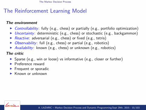
The environmentI Controllability : fully (e.g., chess) or partially (e.g., portfolio optimization)I Uncertainty : deterministic (e.g., chess) or stochastic (e.g., backgammon)I Reactive: adversarial (e.g., chess) or fixed (e.g., tetris)I Observability : full (e.g., chess) or partial (e.g., robotics)I Availability : known (e.g., chess) or unknown (e.g., robotics)
The criticI Sparse (e.g., win or loose) vs informative (e.g., closer or further)I Preference rewardI Frequent or sporadicI Known or unknown
The agentI Open loop controlI Close loop control (i.e., adaptive)I Non-stationary close loop control (i.e., learning)
A. LAZARIC – Markov Decision Process and Dynamic Programming Sept 29th, 2015 - 15/103
The Markov Decision Process
The Reinforcement Learning Model
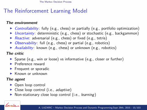
The environmentI Controllability : fully (e.g., chess) or partially (e.g., portfolio optimization)I Uncertainty : deterministic (e.g., chess) or stochastic (e.g., backgammon)I Reactive: adversarial (e.g., chess) or fixed (e.g., tetris)I Observability : full (e.g., chess) or partial (e.g., robotics)I Availability : known (e.g., chess) or unknown (e.g., robotics)
The criticI Sparse (e.g., win or loose) vs informative (e.g., closer or further)I Preference rewardI Frequent or sporadicI Known or unknown
The agentI Open loop controlI Close loop control (i.e., adaptive)I Non-stationary close loop control (i.e., learning)
A. LAZARIC – Markov Decision Process and Dynamic Programming Sept 29th, 2015 - 15/103
The Markov Decision Process
The Reinforcement Learning Model
The environmentI Controllability : fully (e.g., chess) or partially (e.g., portfolio optimization)I Uncertainty : deterministic (e.g., chess) or stochastic (e.g., backgammon)I Reactive: adversarial (e.g., chess) or fixed (e.g., tetris)I Observability : full (e.g., chess) or partial (e.g., robotics)I Availability : known (e.g., chess) or unknown (e.g., robotics)
The criticI Sparse (e.g., win or loose) vs informative (e.g., closer or further)I Preference rewardI Frequent or sporadicI Known or unknown
The agentI Open loop controlI Close loop control (i.e., adaptive)I Non-stationary close loop control (i.e., learning)
A. LAZARIC – Markov Decision Process and Dynamic Programming Sept 29th, 2015 - 15/103
The Markov Decision Process
Markov Chains
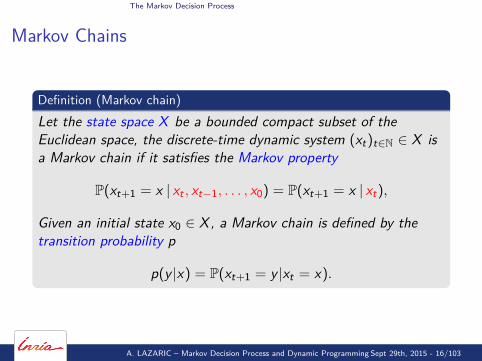
Definition (Markov chain)Let the state space X be a bounded compact subset of theEuclidean space, the discrete-time dynamic system (xt)t∈N ∈ X isa Markov chain if it satisfies the Markov property
P(xt+1 = x | xt , xt−1, . . . , x0) = P(xt+1 = x | xt),
Given an initial state x0 ∈ X, a Markov chain is defined by thetransition probability p
p(y |x) = P(xt+1 = y |xt = x).
A. LAZARIC – Markov Decision Process and Dynamic Programming Sept 29th, 2015 - 16/103
The Markov Decision Process
Markov Decision Process
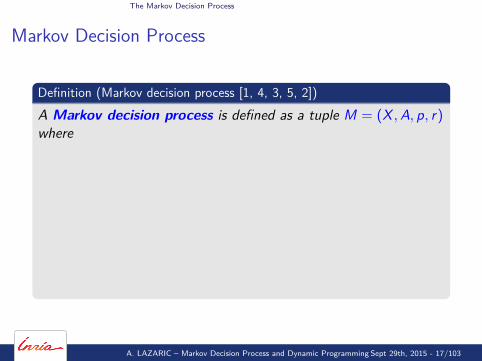
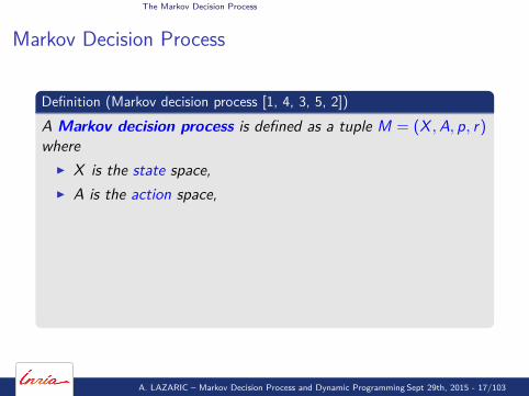
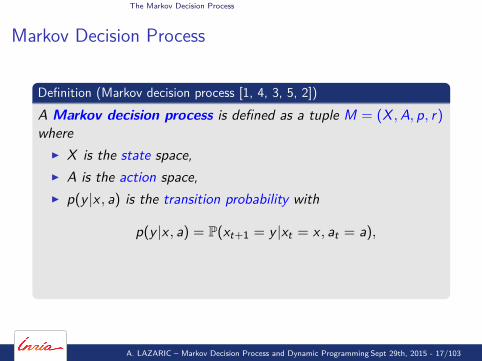
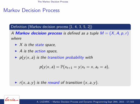
Definition (Markov decision process [1, 4, 3, 5, 2])A Markov decision process is defined as a tuple M = (X ,A, p, r)where
I X is the state space,I A is the action space,I p(y |x , a) is the transition probability with
p(y |x , a) = P(xt+1 = y |xt = x , at = a),
I r(x , a, y) is the reward of transition (x , a, y).
A. LAZARIC – Markov Decision Process and Dynamic Programming Sept 29th, 2015 - 17/103

The Markov Decision Process
Markov Decision Process
Definition (Markov decision process [1, 4, 3, 5, 2])A Markov decision process is defined as a tuple M = (X ,A, p, r)whereI X is the state space,
I A is the action space,I p(y |x , a) is the transition probability with
p(y |x , a) = P(xt+1 = y |xt = x , at = a),
I r(x , a, y) is the reward of transition (x , a, y).
A. LAZARIC – Markov Decision Process and Dynamic Programming Sept 29th, 2015 - 17/103
The Markov Decision Process
Markov Decision Process
Definition (Markov decision process [1, 4, 3, 5, 2])A Markov decision process is defined as a tuple M = (X ,A, p, r)whereI X is the state space,I A is the action space,
I p(y |x , a) is the transition probability with
p(y |x , a) = P(xt+1 = y |xt = x , at = a),
I r(x , a, y) is the reward of transition (x , a, y).
A. LAZARIC – Markov Decision Process and Dynamic Programming Sept 29th, 2015 - 17/103
The Markov Decision Process
Markov Decision Process
Definition (Markov decision process [1, 4, 3, 5, 2])A Markov decision process is defined as a tuple M = (X ,A, p, r)whereI X is the state space,I A is the action space,I p(y |x , a) is the transition probability with
p(y |x , a) = P(xt+1 = y |xt = x , at = a),
I r(x , a, y) is the reward of transition (x , a, y).
A. LAZARIC – Markov Decision Process and Dynamic Programming Sept 29th, 2015 - 17/103

The Markov Decision Process
Markov Decision Process: the Assumptions
Time assumption: time is discrete
t → t + 1
Possible relaxationsI Identify the proper time granularityI Most of MDP literature extends to continuous time
A. LAZARIC – Markov Decision Process and Dynamic Programming Sept 29th, 2015 - 18/103
The Markov Decision Process
Markov Decision Process: the Assumptions
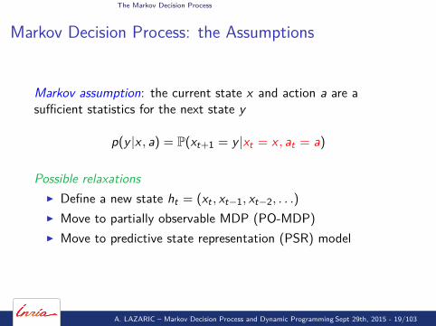
Markov assumption: the current state x and action a are asufficient statistics for the next state y
p(y |x , a) = P(xt+1 = y |xt = x , at = a)
Possible relaxationsI Define a new state ht = (xt , xt−1, xt−2, . . .)
I Move to partially observable MDP (PO-MDP)I Move to predictive state representation (PSR) model
A. LAZARIC – Markov Decision Process and Dynamic Programming Sept 29th, 2015 - 19/103
The Markov Decision Process
Markov Decision Process: the Assumptions
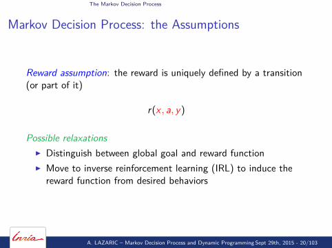
Reward assumption: the reward is uniquely defined by a transition(or part of it)
r(x , a, y)
Possible relaxationsI Distinguish between global goal and reward functionI Move to inverse reinforcement learning (IRL) to induce the
reward function from desired behaviors
A. LAZARIC – Markov Decision Process and Dynamic Programming Sept 29th, 2015 - 20/103

The Markov Decision Process
Markov Decision Process: the Assumptions
Stationarity assumption: the dynamics and reward do not changeover time
p(y |x , a) = P(xt+1 = y |xt = x , at = a) r(x , a, y)
Possible relaxationsI Identify and remove the non-stationary components (e.g.,
cyclo-stationary dynamics)I Identify the time-scale of the changes
A. LAZARIC – Markov Decision Process and Dynamic Programming Sept 29th, 2015 - 21/103

The Markov Decision Process
Question
Is the MDP formalism powerful enough?
⇒ Let’s try!
A. LAZARIC – Markov Decision Process and Dynamic Programming Sept 29th, 2015 - 22/103
The Markov Decision Process
Example: the Retail Store Management Problem
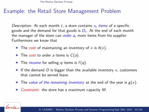
Description. At each month t, a store contains xt items of a specificgoods and the demand for that goods is Dt . At the end of each monththe manager of the store can order at more items from his supplier.Furthermore we know thatI The cost of maintaining an inventory of x is h(x).I The cost to order a items is C(a).I The income for selling q items is f (q).I If the demand D is bigger than the available inventory x , customers
that cannot be served leave.I The value of the remaining inventory at the end of the year is g(x).I Constraint: the store has a maximum capacity M.
A. LAZARIC – Markov Decision Process and Dynamic Programming Sept 29th, 2015 - 23/103

The Markov Decision Process
Example: the Retail Store Management Problem
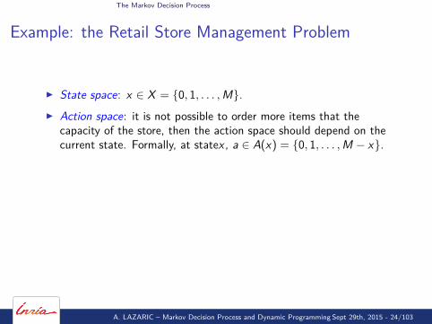
I State space: x ∈ X = {0, 1, . . . ,M}.
I Action space: it is not possible to order more items that thecapacity of the store, then the action space should depend on thecurrent state. Formally, at statex , a ∈ A(x) = {0, 1, . . . ,M − x}.
I Dynamics: xt+1 = [xt + at − Dt ]+.Problem: the dynamics should be Markov and stationary!
I The demand Dt is stochastic and time-independent. Formally,Dt
i.i.d.∼ D.I Reward : rt = −C(at)− h(xt + at) + f ([xt + at − xt+1]+).
A. LAZARIC – Markov Decision Process and Dynamic Programming Sept 29th, 2015 - 24/103
The Markov Decision Process
Example: the Retail Store Management Problem
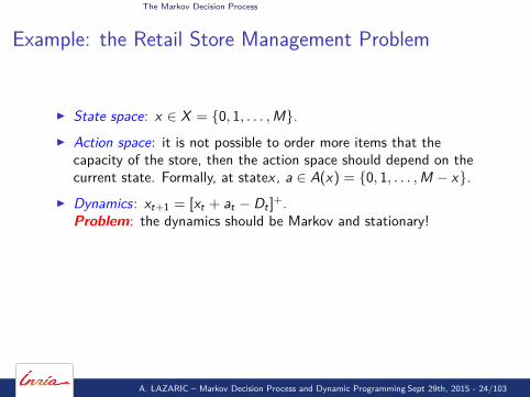
I State space: x ∈ X = {0, 1, . . . ,M}.I Action space: it is not possible to order more items that the
capacity of the store, then the action space should depend on thecurrent state. Formally, at statex , a ∈ A(x) = {0, 1, . . . ,M − x}.
I Dynamics: xt+1 = [xt + at − Dt ]+.Problem: the dynamics should be Markov and stationary!
I The demand Dt is stochastic and time-independent. Formally,Dt
i.i.d.∼ D.I Reward : rt = −C(at)− h(xt + at) + f ([xt + at − xt+1]+).
A. LAZARIC – Markov Decision Process and Dynamic Programming Sept 29th, 2015 - 24/103
The Markov Decision Process
Example: the Retail Store Management Problem
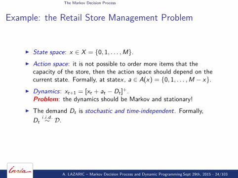
I State space: x ∈ X = {0, 1, . . . ,M}.I Action space: it is not possible to order more items that the
capacity of the store, then the action space should depend on thecurrent state. Formally, at statex , a ∈ A(x) = {0, 1, . . . ,M − x}.
I Dynamics: xt+1 = [xt + at − Dt ]+.Problem: the dynamics should be Markov and stationary!
I The demand Dt is stochastic and time-independent. Formally,Dt
i.i.d.∼ D.I Reward : rt = −C(at)− h(xt + at) + f ([xt + at − xt+1]+).
A. LAZARIC – Markov Decision Process and Dynamic Programming Sept 29th, 2015 - 24/103
The Markov Decision Process
Example: the Retail Store Management Problem
I State space: x ∈ X = {0, 1, . . . ,M}.I Action space: it is not possible to order more items that the
capacity of the store, then the action space should depend on thecurrent state. Formally, at statex , a ∈ A(x) = {0, 1, . . . ,M − x}.
I Dynamics: xt+1 = [xt + at − Dt ]+.Problem: the dynamics should be Markov and stationary!
I The demand Dt is stochastic and time-independent. Formally,Dt
i.i.d.∼ D.
I Reward : rt = −C(at)− h(xt + at) + f ([xt + at − xt+1]+).
A. LAZARIC – Markov Decision Process and Dynamic Programming Sept 29th, 2015 - 24/103

The Markov Decision Process
Example: the Retail Store Management Problem
I State space: x ∈ X = {0, 1, . . . ,M}.I Action space: it is not possible to order more items that the
capacity of the store, then the action space should depend on thecurrent state. Formally, at statex , a ∈ A(x) = {0, 1, . . . ,M − x}.
I Dynamics: xt+1 = [xt + at − Dt ]+.Problem: the dynamics should be Markov and stationary!
I The demand Dt is stochastic and time-independent. Formally,Dt
i.i.d.∼ D.I Reward : rt = −C(at)− h(xt + at) + f ([xt + at − xt+1]+).
A. LAZARIC – Markov Decision Process and Dynamic Programming Sept 29th, 2015 - 24/103
The Markov Decision Process
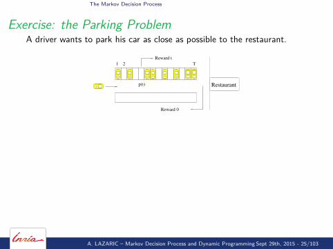
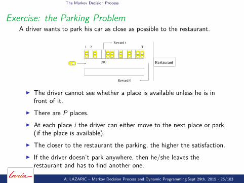
Exercise: the Parking ProblemA driver wants to park his car as close as possible to the restaurant.
T21
Reward t
p(t)
Reward 0
Restaurant
I The driver cannot see whether a place is available unless he is infront of it.
I There are P places.I At each place i the driver can either move to the next place or park
(if the place is available).I The closer to the restaurant the parking, the higher the satisfaction.I If the driver doesn’t park anywhere, then he/she leaves the
restaurant and has to find another one.
A. LAZARIC – Markov Decision Process and Dynamic Programming Sept 29th, 2015 - 25/103
The Markov Decision Process
Policy
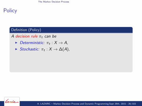
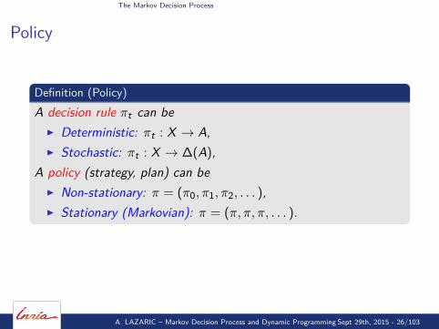
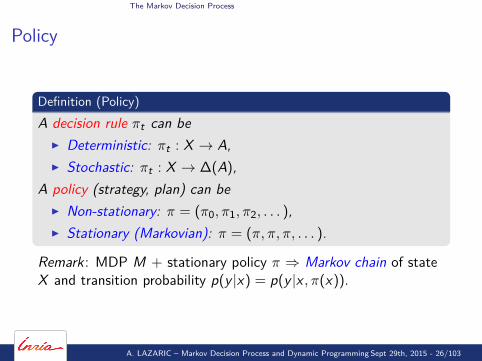
Definition (Policy)A decision rule πt can beI Deterministic: πt : X → A,I Stochastic: πt : X → ∆(A),
A policy (strategy, plan) can beI Non-stationary: π = (π0, π1, π2, . . . ),I Stationary (Markovian): π = (π, π, π, . . . ).
Remark: MDP M + stationary policy π ⇒ Markov chain of stateX and transition probability p(y |x) = p(y |x , π(x)).
A. LAZARIC – Markov Decision Process and Dynamic Programming Sept 29th, 2015 - 26/103
The Markov Decision Process
Policy
Definition (Policy)A decision rule πt can beI Deterministic: πt : X → A,I Stochastic: πt : X → ∆(A),
A policy (strategy, plan) can beI Non-stationary: π = (π0, π1, π2, . . . ),I Stationary (Markovian): π = (π, π, π, . . . ).
Remark: MDP M + stationary policy π ⇒ Markov chain of stateX and transition probability p(y |x) = p(y |x , π(x)).
A. LAZARIC – Markov Decision Process and Dynamic Programming Sept 29th, 2015 - 26/103
The Markov Decision Process
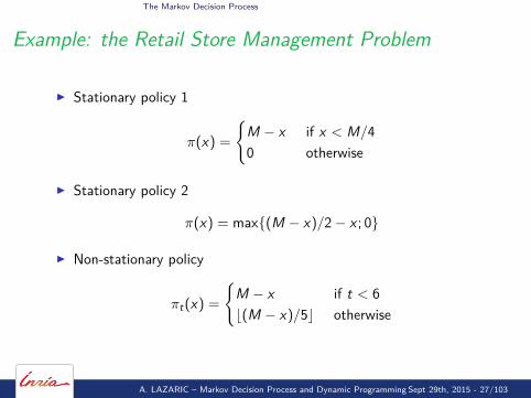
Example: the Retail Store Management Problem
I Stationary policy 1
π(x) =
{M − x if x < M/40 otherwise
I Stationary policy 2
π(x) = max{(M − x)/2− x ; 0}
I Non-stationary policy
πt(x) =
{M − x if t < 6b(M − x)/5c otherwise
A. LAZARIC – Markov Decision Process and Dynamic Programming Sept 29th, 2015 - 27/103
The Markov Decision Process
How to model an RL problem
The Markov Decision Process
The Model
Value Functions
A. LAZARIC – Markov Decision Process and Dynamic Programming Sept 29th, 2015 - 28/103
The Markov Decision Process
Question
How do we evaluate a policy and compare two policies?
⇒ Value function!
A. LAZARIC – Markov Decision Process and Dynamic Programming Sept 29th, 2015 - 29/103
The Markov Decision Process
Optimization over Time Horizon
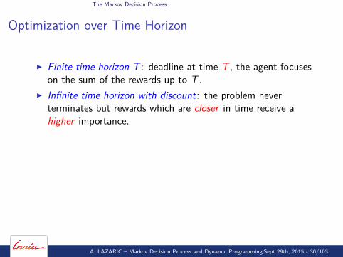
I Finite time horizon T : deadline at time T , the agent focuseson the sum of the rewards up to T .
I Infinite time horizon with discount: the problem neverterminates but rewards which are closer in time receive ahigher importance.
I Infinite time horizon with terminal state: the problem neverterminates but the agent will eventually reach a terminationstate.
I Infinite time horizon with average reward : the problem neverterminates but the agent only focuses on the (expected)average of the rewards.
A. LAZARIC – Markov Decision Process and Dynamic Programming Sept 29th, 2015 - 30/103
The Markov Decision Process
Optimization over Time Horizon
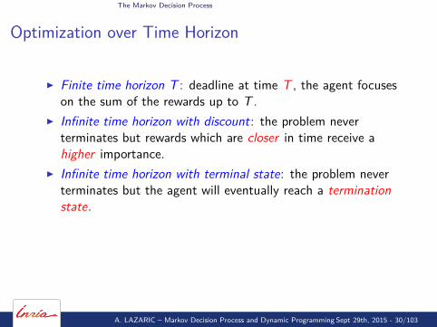
I Finite time horizon T : deadline at time T , the agent focuseson the sum of the rewards up to T .
I Infinite time horizon with discount: the problem neverterminates but rewards which are closer in time receive ahigher importance.
I Infinite time horizon with terminal state: the problem neverterminates but the agent will eventually reach a terminationstate.
I Infinite time horizon with average reward : the problem neverterminates but the agent only focuses on the (expected)average of the rewards.
A. LAZARIC – Markov Decision Process and Dynamic Programming Sept 29th, 2015 - 30/103
The Markov Decision Process
Optimization over Time Horizon
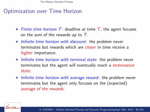
I Finite time horizon T : deadline at time T , the agent focuseson the sum of the rewards up to T .
I Infinite time horizon with discount: the problem neverterminates but rewards which are closer in time receive ahigher importance.
I Infinite time horizon with terminal state: the problem neverterminates but the agent will eventually reach a terminationstate.
I Infinite time horizon with average reward : the problem neverterminates but the agent only focuses on the (expected)average of the rewards.
A. LAZARIC – Markov Decision Process and Dynamic Programming Sept 29th, 2015 - 30/103
The Markov Decision Process
Optimization over Time Horizon
I Finite time horizon T : deadline at time T , the agent focuseson the sum of the rewards up to T .
I Infinite time horizon with discount: the problem neverterminates but rewards which are closer in time receive ahigher importance.
I Infinite time horizon with terminal state: the problem neverterminates but the agent will eventually reach a terminationstate.
I Infinite time horizon with average reward : the problem neverterminates but the agent only focuses on the (expected)average of the rewards.
A. LAZARIC – Markov Decision Process and Dynamic Programming Sept 29th, 2015 - 30/103
The Markov Decision Process
State Value Function
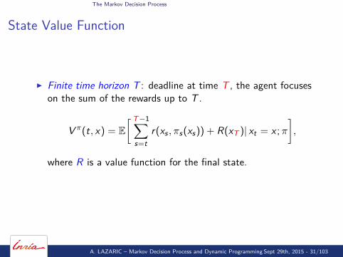
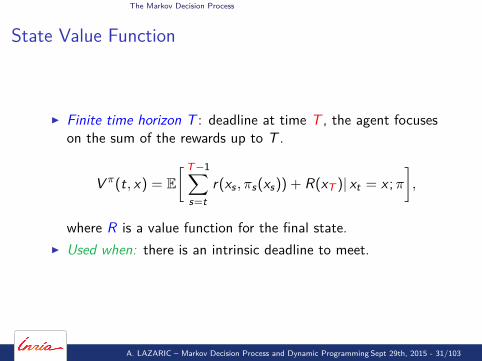
I Finite time horizon T : deadline at time T , the agent focuseson the sum of the rewards up to T .
V π(t, x) = E[ T−1∑
s=tr(xs , πs(xs)) + R(xT )| xt = x ;π
],
where R is a value function for the final state.
I Used when: there is an intrinsic deadline to meet.
A. LAZARIC – Markov Decision Process and Dynamic Programming Sept 29th, 2015 - 31/103
The Markov Decision Process
State Value Function
I Finite time horizon T : deadline at time T , the agent focuseson the sum of the rewards up to T .
V π(t, x) = E[ T−1∑
s=tr(xs , πs(xs)) + R(xT )| xt = x ;π
],
where R is a value function for the final state.I Used when: there is an intrinsic deadline to meet.
A. LAZARIC – Markov Decision Process and Dynamic Programming Sept 29th, 2015 - 31/103
The Markov Decision Process
State Value Function
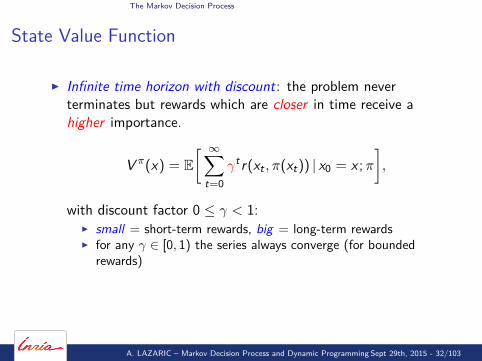
I Infinite time horizon with discount: the problem neverterminates but rewards which are closer in time receive ahigher importance.
V π(x) = E[ ∞∑
t=0γtr(xt , π(xt)) | x0 = x ;π
],
with discount factor 0 ≤ γ < 1:I small = short-term rewards, big = long-term rewardsI for any γ ∈ [0, 1) the series always converge (for bounded
rewards)
I Used when: there is uncertainty about the deadline and/or anintrinsic definition of discount.
A. LAZARIC – Markov Decision Process and Dynamic Programming Sept 29th, 2015 - 32/103
The Markov Decision Process
State Value Function
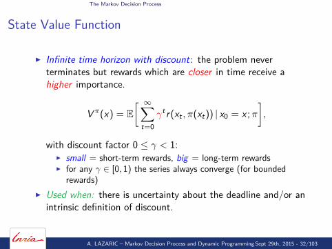
I Infinite time horizon with discount: the problem neverterminates but rewards which are closer in time receive ahigher importance.
V π(x) = E[ ∞∑
t=0γtr(xt , π(xt)) | x0 = x ;π
],
with discount factor 0 ≤ γ < 1:I small = short-term rewards, big = long-term rewardsI for any γ ∈ [0, 1) the series always converge (for bounded
rewards)I Used when: there is uncertainty about the deadline and/or an
intrinsic definition of discount.
A. LAZARIC – Markov Decision Process and Dynamic Programming Sept 29th, 2015 - 32/103

The Markov Decision Process
State Value Function
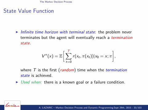
I Infinite time horizon with terminal state: the problem neverterminates but the agent will eventually reach a terminationstate.
V π(x) = E[ T∑
t=0r(xt , π(xt))|x0 = x ;π
],
where T is the first (random) time when the terminationstate is achieved.
I Used when: there is a known goal or a failure condition.
A. LAZARIC – Markov Decision Process and Dynamic Programming Sept 29th, 2015 - 33/103
The Markov Decision Process
State Value Function
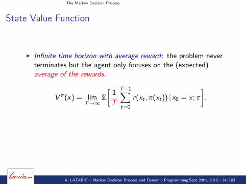
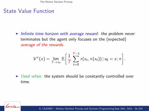
I Infinite time horizon with average reward : the problem neverterminates but the agent only focuses on the (expected)average of the rewards.
V π(x) = limT→∞
E[
1T
T−1∑t=0
r(xt , π(xt)) | x0 = x ;π
].
I Used when: the system should be constantly controlled overtime.
A. LAZARIC – Markov Decision Process and Dynamic Programming Sept 29th, 2015 - 34/103
The Markov Decision Process
State Value Function
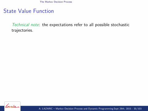
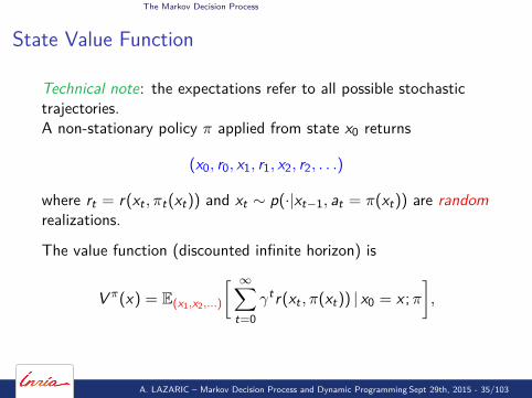
Technical note: the expectations refer to all possible stochastictrajectories.
A non-stationary policy π applied from state x0 returns
(x0, r0, x1, r1, x2, r2, . . .)
where rt = r(xt , πt(xt)) and xt ∼ p(·|xt−1, at = π(xt)) are randomrealizations.
The value function (discounted infinite horizon) is
V π(x) = E(x1,x2,...)
[ ∞∑t=0
γtr(xt , π(xt)) | x0 = x ;π
],
A. LAZARIC – Markov Decision Process and Dynamic Programming Sept 29th, 2015 - 35/103
The Markov Decision Process
State Value Function
Technical note: the expectations refer to all possible stochastictrajectories.A non-stationary policy π applied from state x0 returns
(x0, r0, x1, r1, x2, r2, . . .)
where rt = r(xt , πt(xt)) and xt ∼ p(·|xt−1, at = π(xt)) are randomrealizations.
The value function (discounted infinite horizon) is
V π(x) = E(x1,x2,...)
[ ∞∑t=0
γtr(xt , π(xt)) | x0 = x ;π
],
A. LAZARIC – Markov Decision Process and Dynamic Programming Sept 29th, 2015 - 35/103
The Markov Decision Process
Example: the Retail Store Management Problem
Simulation
A. LAZARIC – Markov Decision Process and Dynamic Programming Sept 29th, 2015 - 36/103
The Markov Decision Process
Optimal Value Function
Definition (Optimal policy and optimal value function)
The solution to an MDP is an optimal policy π∗ satisfying
π∗ ∈ arg maxπ∈Π
V π
in all the states x ∈ X, where Π is some policy set of interest.
The corresponding value function is the optimal value function
V ∗ = V π∗
A. LAZARIC – Markov Decision Process and Dynamic Programming Sept 29th, 2015 - 37/103

The Markov Decision Process
Optimal Value Function
Remarks1. π∗ ∈ arg max(·) and not π∗ = arg max(·) because an MDP
may admit more than one optimal policy
2. π∗ achieves the largest possible value function in every state
3. there always exists an optimal deterministic policy
4. expect for problems with a finite horizon, there always existsan optimal stationary policy
A. LAZARIC – Markov Decision Process and Dynamic Programming Sept 29th, 2015 - 38/103
The Markov Decision Process
Summary
1. MDP is a powerful model for interaction between an agentand a stochastic environment
2. The value function defines the objective to optimize
A. LAZARIC – Markov Decision Process and Dynamic Programming Sept 29th, 2015 - 39/103
The Markov Decision Process
Limitations
1. All the previous value functions define an objective inexpectation
2. Other utility functions may be used
3. Risk measures could be integrated but they may induce“weird” problems and make the solution more difficult
A. LAZARIC – Markov Decision Process and Dynamic Programming Sept 29th, 2015 - 40/103
The Markov Decision Process
How to solve exactly an MDP
Dynamic Programming
Bellman Equations
Value Iteration
Policy Iteration
A. LAZARIC – Markov Decision Process and Dynamic Programming Sept 29th, 2015 - 41/103
The Markov Decision Process
How to solve exactly an MDP
Dynamic Programming
Bellman Equations
Value Iteration
Policy Iteration
A. LAZARIC – Markov Decision Process and Dynamic Programming Sept 29th, 2015 - 41/103
The Markov Decision Process
Notice
From now on we mostly work on thediscounted infinite horizon setting.
Most results smoothly extend to other settings.
A. LAZARIC – Markov Decision Process and Dynamic Programming Sept 29th, 2015 - 42/103
The Markov Decision Process
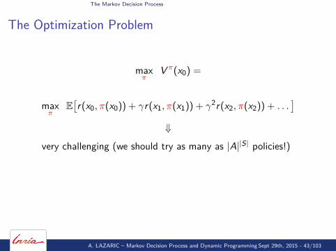
The Optimization Problem
maxπ
V π(x0) =
maxπ
E[r(x0, π(x0)) + γr(x1, π(x1)) + γ2r(x2, π(x2)) + . . .
]⇓
very challenging (we should try as many as |A||S| policies!)
⇓
we need to leverage the structure of the MDPto simplify the optimization problem
A. LAZARIC – Markov Decision Process and Dynamic Programming Sept 29th, 2015 - 43/103
The Markov Decision Process
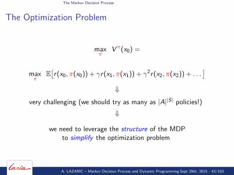
The Optimization Problem
maxπ
V π(x0) =
maxπ
E[r(x0, π(x0)) + γr(x1, π(x1)) + γ2r(x2, π(x2)) + . . .
]⇓
very challenging (we should try as many as |A||S| policies!)⇓
we need to leverage the structure of the MDPto simplify the optimization problem
A. LAZARIC – Markov Decision Process and Dynamic Programming Sept 29th, 2015 - 43/103
The Markov Decision Process
How to solve exactly an MDP
Dynamic Programming
Bellman Equations
Value Iteration
Policy Iteration
A. LAZARIC – Markov Decision Process and Dynamic Programming Sept 29th, 2015 - 44/103

The Markov Decision Process
The Bellman Equation
PropositionFor any stationary policy π = (π, π, . . . ), the state value functionat a state x ∈ X satisfies the Bellman equation:
V π(x) = r(x , π(x)) + γ∑
yp(y |x , π(x))V π(y).
A. LAZARIC – Markov Decision Process and Dynamic Programming Sept 29th, 2015 - 45/103

The Markov Decision Process
The Bellman Equation
Proof.For any policy π,
V π(x) = E[∑
t≥0γtr(xt , π(xt)) | x0 = x ;π
]= r(x , π(x)) + E
[∑t≥1
γtr(xt , π(xt)) | x0 = x ;π]
= r(x , π(x))
+ γ∑
yP(x1 = y | x0 = x ;π(x0))E
[∑t≥1
γt−1r(xt , π(xt)) | x1 = y ;π]
= r(x , π(x)) + γ∑
yp(y |x , π(x))V π(y).
�
A. LAZARIC – Markov Decision Process and Dynamic Programming Sept 29th, 2015 - 46/103

The Markov Decision Process
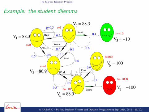
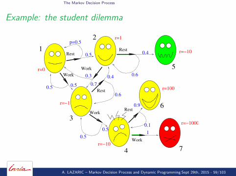
Example: the student dilemma
Work
Work
Work
Work
RestRest
Rest
Rest
p=0.5
0.4
0.3
0.7
0.5
0.50.5
0.5
0.4
0.6
0.6
10.5
r=1
r=−1000
r=0
r=−10
r=100
r=−10
0.9
0.1
r=−1
1
2
3
4
5
6
7
A. LAZARIC – Markov Decision Process and Dynamic Programming Sept 29th, 2015 - 47/103
The Markov Decision Process
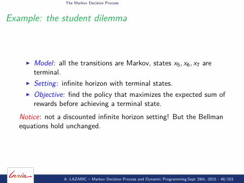
Example: the student dilemma
I Model : all the transitions are Markov, states x5, x6, x7 areterminal.
I Setting : infinite horizon with terminal states.I Objective: find the policy that maximizes the expected sum of
rewards before achieving a terminal state.
Notice: not a discounted infinite horizon setting! But the Bellmanequations hold unchanged.
A. LAZARIC – Markov Decision Process and Dynamic Programming Sept 29th, 2015 - 48/103

The Markov Decision Process
Example: the student dilemma
Work
Work
Work
Work
RestRest
Rest
Rest
p=0.5
0.4
0.3
0.7
0.5
0.50.5
0.5
0.4
0.6
0.6
10.5
r=−1000
r=0
r=−10
r=100
0.9
0.1
r=−1
V = 88.31
V = 86.93
r=−10
V = 88.94
r=1V = 88.3
2
V = −105
V = 1006
V = −10007
A. LAZARIC – Markov Decision Process and Dynamic Programming Sept 29th, 2015 - 49/103
The Markov Decision Process
Example: the student dilemma
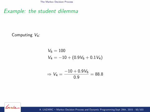
Computing V4:
V6 = 100V4 = −10 + (0.9V6 + 0.1V4)
⇒ V4 =−10 + 0.9V6
0.9 = 88.8
A. LAZARIC – Markov Decision Process and Dynamic Programming Sept 29th, 2015 - 50/103
The Markov Decision Process
Example: the student dilemma
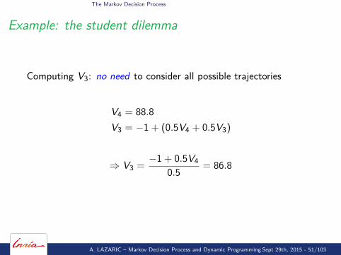
Computing V3: no need to consider all possible trajectories
V4 = 88.8V3 = −1 + (0.5V4 + 0.5V3)
⇒ V3 =−1 + 0.5V4
0.5 = 86.8
and so on for the rest...
A. LAZARIC – Markov Decision Process and Dynamic Programming Sept 29th, 2015 - 51/103
The Markov Decision Process
Example: the student dilemma
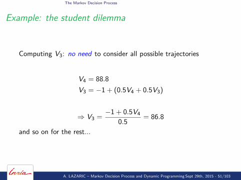
Computing V3: no need to consider all possible trajectories
V4 = 88.8V3 = −1 + (0.5V4 + 0.5V3)
⇒ V3 =−1 + 0.5V4
0.5 = 86.8
and so on for the rest...
A. LAZARIC – Markov Decision Process and Dynamic Programming Sept 29th, 2015 - 51/103

The Markov Decision Process
The Optimal Bellman Equation
Bellman’s Principle of Optimality [1]:“An optimal policy has the property that, whatever theinitial state and the initial decision are, the remainingdecisions must constitute an optimal policy with regardto the state resulting from the first decision.”
A. LAZARIC – Markov Decision Process and Dynamic Programming Sept 29th, 2015 - 52/103
The Markov Decision Process
The Optimal Bellman Equation
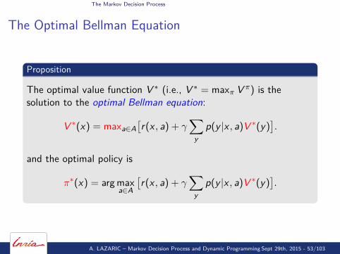
Proposition
The optimal value function V ∗ (i.e., V ∗ = maxπ V π) is thesolution to the optimal Bellman equation:
V ∗(x) = maxa∈A[r(x , a) + γ
∑y
p(y |x , a)V ∗(y)].
and the optimal policy is
π∗(x) = arg maxa∈A
[r(x , a) + γ
∑y
p(y |x , a)V ∗(y)].
A. LAZARIC – Markov Decision Process and Dynamic Programming Sept 29th, 2015 - 53/103
The Markov Decision Process
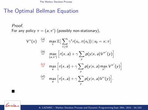
The Optimal Bellman Equation
Proof.For any policy π = (a, π′) (possibly non-stationary),
V ∗(x)(a)= max
πE[∑
t≥0γtr(xt , π(xt)) | x0 = x ;π
](b)= max
(a,π′)
[r(x , a) + γ
∑y
p(y |x , a)V π′(y)]
(c)= max
a
[r(x , a) + γ
∑y
p(y |x , a) maxπ′
V π′(y)]
(d)= max
a
[r(x , a) + γ
∑y
p(y |x , a)V ∗(y)].
�
A. LAZARIC – Markov Decision Process and Dynamic Programming Sept 29th, 2015 - 54/103
The Markov Decision Process
System of Equations
The Bellman equation
V π(x) = r(x , π(x)) + γ∑
yp(y |x , π(x))V π(y).
is a linear system of equations with N unknowns and N linearconstraints.
A. LAZARIC – Markov Decision Process and Dynamic Programming Sept 29th, 2015 - 55/103
The Markov Decision Process
Example: the student dilemma
Work
Work
Work
Work
RestRest
Rest
Rest
p=0.5
0.4
0.3
0.7
0.5
0.50.5
0.5
0.4
0.6
0.6
10.5
r=−1000
r=0
r=−10
r=100
0.9
0.1
r=−1
V = 88.31
V = 86.93
r=−10
V = 88.94
r=1V = 88.3
2
V = −105
V = 1006
V = −10007
A. LAZARIC – Markov Decision Process and Dynamic Programming Sept 29th, 2015 - 56/103
The Markov Decision Process
Example: the student dilemma
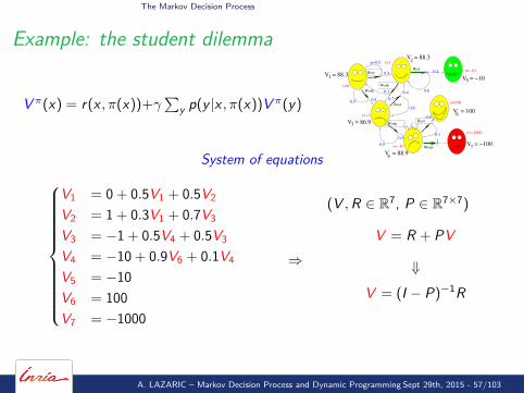
V π(x) = r(x , π(x))+γ∑
y p(y |x , π(x))V π(y)
Work
Work
Work
Work
RestRest
Rest
Rest
p=0.5
0.4
0.3
0.7
0.5
0.50.5
0.5
0.4
0.6
0.6
10.5
r=−1000
r=0
r=−10
r=100
0.9
0.1
r=−1
V = 88.31
V = 86.93
r=−10
V = 88.94
r=1V = 88.3
2
V = −105
V = 1006
V = −10007
System of equations
V1 = 0 + 0.5V1 + 0.5V2
V2 = 1 + 0.3V1 + 0.7V3
V3 = −1 + 0.5V4 + 0.5V3
V4 = −10 + 0.9V6 + 0.1V4
V5 = −10V6 = 100V7 = −1000
⇒
(V ,R ∈ R7, P ∈ R7×7)
V = R + PV
⇓
V = (I − P)−1R
A. LAZARIC – Markov Decision Process and Dynamic Programming Sept 29th, 2015 - 57/103

The Markov Decision Process
System of Equations
The optimal Bellman equation
V ∗(x) = maxa∈A[r(x , a) + γ
∑y
p(y |x , a)V ∗(y)].
is a (highly) non-linear system of equations with N unknowns andN non-linear constraints (i.e., the max operator).
A. LAZARIC – Markov Decision Process and Dynamic Programming Sept 29th, 2015 - 58/103
The Markov Decision Process
Example: the student dilemma
Work
Work
Work
Work
RestRest
Rest
Rest
p=0.5
0.4
0.3
0.7
0.5
0.50.5
0.5
0.4
0.6
0.6
10.5
r=1
r=−1000
r=0
r=−10
r=100
r=−10
0.9
0.1
r=−1
1
2
3
4
5
6
7
A. LAZARIC – Markov Decision Process and Dynamic Programming Sept 29th, 2015 - 59/103
The Markov Decision Process
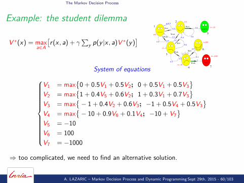
Example: the student dilemma
V ∗(x) = maxa∈A
[r(x , a) + γ
∑y p(y |x , a)V ∗(y)
]Work
Work
Work
Work
RestRest
Rest
Rest
p=0.5
0.4
0.3
0.7
0.5
0.50.5
0.5
0.4
0.6
0.6
10.5
r=1
r=−1000
r=0
r=−10
r=100
r=−10
0.9
0.1
r=−1
1
2
3
4
5
6
7System of equations
V1 = max{
0 + 0.5V1 + 0.5V2; 0 + 0.5V1 + 0.5V3}
V2 = max{
1 + 0.4V5 + 0.6V2; 1 + 0.3V1 + 0.7V3}
V3 = max{− 1 + 0.4V2 + 0.6V3; −1 + 0.5V4 + 0.5V3
}V4 = max
{− 10 + 0.9V6 + 0.1V4; −10 + V7
}V5 = −10V6 = 100V7 = −1000
⇒ too complicated, we need to find an alternative solution.
A. LAZARIC – Markov Decision Process and Dynamic Programming Sept 29th, 2015 - 60/103
The Markov Decision Process
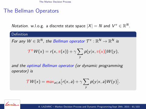
The Bellman Operators
Notation. w.l.o.g. a discrete state space |X | = N and V π ∈ RN .
Definition
For any W ∈ RN , the Bellman operator T π : RN → RN is
T πW (x) = r(x , π(x)) + γ∑
yp(y |x , π(x))W (y),
and the optimal Bellman operator (or dynamic programmingoperator) is
TW (x) = maxa∈A[r(x , a) + γ
∑y
p(y |x , a)W (y)].
A. LAZARIC – Markov Decision Process and Dynamic Programming Sept 29th, 2015 - 61/103
The Markov Decision Process
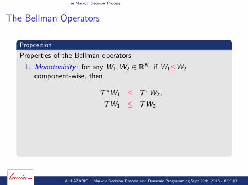
The Bellman Operators
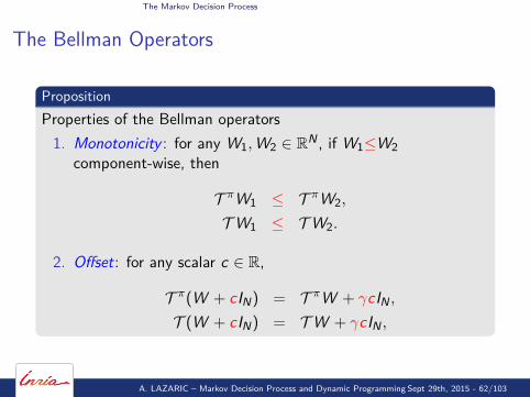
PropositionProperties of the Bellman operators
1. Monotonicity : for any W1,W2 ∈ RN , if W1≤W2component-wise, then
T πW1 ≤ T πW2,
TW1 ≤ TW2.
2. Offset: for any scalar c ∈ R,
T π(W + cIN) = T πW + γcIN ,T (W + cIN) = TW + γcIN ,
A. LAZARIC – Markov Decision Process and Dynamic Programming Sept 29th, 2015 - 62/103
The Markov Decision Process
The Bellman Operators
PropositionProperties of the Bellman operators
1. Monotonicity : for any W1,W2 ∈ RN , if W1≤W2component-wise, then
T πW1 ≤ T πW2,
TW1 ≤ TW2.
2. Offset: for any scalar c ∈ R,
T π(W + cIN) = T πW + γcIN ,T (W + cIN) = TW + γcIN ,
A. LAZARIC – Markov Decision Process and Dynamic Programming Sept 29th, 2015 - 62/103
The Markov Decision Process
The Bellman OperatorsProposition
3. Contraction in L∞-norm: for any W1,W2 ∈ RN
||T πW1 − T πW2||∞ ≤ γ||W1 −W2||∞,||TW1 − TW2||∞ ≤ γ||W1 −W2||∞.
4. Fixed point: For any policy π
V π is the unique fixed point of T π,V ∗ is the unique fixed point of T .
Furthermore for any W ∈ RN and any stationary policy π
limk→∞
(T π)kW = V π,
limk→∞
(T )kW = V ∗.
A. LAZARIC – Markov Decision Process and Dynamic Programming Sept 29th, 2015 - 63/103

The Markov Decision Process
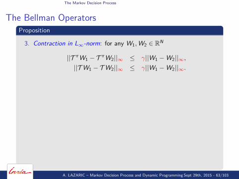
The Bellman OperatorsProposition
3. Contraction in L∞-norm: for any W1,W2 ∈ RN
||T πW1 − T πW2||∞ ≤ γ||W1 −W2||∞,||TW1 − TW2||∞ ≤ γ||W1 −W2||∞.
4. Fixed point: For any policy π
V π is the unique fixed point of T π,V ∗ is the unique fixed point of T .
Furthermore for any W ∈ RN and any stationary policy π
limk→∞
(T π)kW = V π,
limk→∞
(T )kW = V ∗.
A. LAZARIC – Markov Decision Process and Dynamic Programming Sept 29th, 2015 - 63/103
The Markov Decision Process
The Bellman Equation
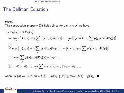
Proof.The contraction property (3) holds since for any x ∈ X we have
|TW1(x)− TW2(x)|
=∣∣∣max
a
[r(x , a) + γ
∑y
p(y |x , a)W1(y)]−max
a′
[r(x , a′) + γ
∑y
p(y |x , a′)W2(y)]∣∣∣
(a)
≤ maxa
∣∣∣[r(x , a) + γ∑
yp(y |x , a)W1(y)
]−[r(x , a) + γ
∑y
p(y |x , a)W2(y)]∣∣∣
= γmaxa
∑y
p(y |x , a)|W1(y)−W2(y)|
≤ γ||W1 −W2||∞maxa
∑y
p(y |x , a) = γ||W1 −W2||∞,
where in (a) we used maxa f (a)−maxa′ g(a′) ≤ maxa(f (a)− g(a)). �
A. LAZARIC – Markov Decision Process and Dynamic Programming Sept 29th, 2015 - 64/103
The Markov Decision Process
Exercise: Fixed Point
Revise the Banach fixed point theorem and prove the fixed pointproperty of the Bellman operator.
A. LAZARIC – Markov Decision Process and Dynamic Programming Sept 29th, 2015 - 65/103

Dynamic Programming
How to solve exactly an MDP
Dynamic Programming
Bellman Equations
Value Iteration
Policy Iteration
A. LAZARIC – Markov Decision Process and Dynamic Programming Sept 29th, 2015 - 66/103
Dynamic Programming
Question
How do we compute the value functions / solve an MDP?
⇒ Value/Policy Iteration algorithms!
A. LAZARIC – Markov Decision Process and Dynamic Programming Sept 29th, 2015 - 67/103
Dynamic Programming
System of Equations
The Bellman equation
V π(x) = r(x , π(x)) + γ∑
yp(y |x , π(x))V π(y).
is a linear system of equations with N unknowns and N linearconstraints.
The optimal Bellman equation
V ∗(x) = maxa∈A[r(x , a) + γ
∑y
p(y |x , a)V ∗(y)].
is a (highly) non-linear system of equations with N unknowns andN non-linear constraints (i.e., the max operator).
A. LAZARIC – Markov Decision Process and Dynamic Programming Sept 29th, 2015 - 68/103

Dynamic Programming
System of Equations
The Bellman equation
V π(x) = r(x , π(x)) + γ∑
yp(y |x , π(x))V π(y).
is a linear system of equations with N unknowns and N linearconstraints.The optimal Bellman equation
V ∗(x) = maxa∈A[r(x , a) + γ
∑y
p(y |x , a)V ∗(y)].
is a (highly) non-linear system of equations with N unknowns andN non-linear constraints (i.e., the max operator).
A. LAZARIC – Markov Decision Process and Dynamic Programming Sept 29th, 2015 - 68/103
Dynamic Programming
Value Iteration: the Idea
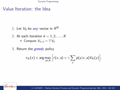
1. Let V0 be any vector in RN
2. At each iteration k = 1, 2, . . . ,KI Compute Vk+1 = T Vk
3. Return the greedy policy
πK (x) ∈ arg maxa∈A
[r(x , a) + γ
∑y
p(y |x , a)VK (y)].
A. LAZARIC – Markov Decision Process and Dynamic Programming Sept 29th, 2015 - 69/103
Dynamic Programming
Value Iteration: the Idea
1. Let V0 be any vector in RN
2. At each iteration k = 1, 2, . . . ,K
I Compute Vk+1 = T Vk
3. Return the greedy policy
πK (x) ∈ arg maxa∈A
[r(x , a) + γ
∑y
p(y |x , a)VK (y)].
A. LAZARIC – Markov Decision Process and Dynamic Programming Sept 29th, 2015 - 69/103

Dynamic Programming
Value Iteration: the Idea
1. Let V0 be any vector in RN
2. At each iteration k = 1, 2, . . . ,KI Compute Vk+1 = T Vk
3. Return the greedy policy
πK (x) ∈ arg maxa∈A
[r(x , a) + γ
∑y
p(y |x , a)VK (y)].
A. LAZARIC – Markov Decision Process and Dynamic Programming Sept 29th, 2015 - 69/103
Dynamic Programming
Value Iteration: the Idea
1. Let V0 be any vector in RN
2. At each iteration k = 1, 2, . . . ,KI Compute Vk+1 = T Vk
3. Return the greedy policy
πK (x) ∈ arg maxa∈A
[r(x , a) + γ
∑y
p(y |x , a)VK (y)].
A. LAZARIC – Markov Decision Process and Dynamic Programming Sept 29th, 2015 - 69/103
Dynamic Programming
Value Iteration: the Guarantees
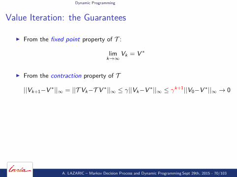
I From the fixed point property of T :
limk→∞
Vk = V ∗
I From the contraction property of T
||Vk+1−V ∗||∞ = ||T Vk−T V ∗||∞ ≤ γ||Vk−V ∗||∞ ≤ γk+1||V0−V ∗||∞ → 0
I Convergence rate. Let ε > 0 and ||r ||∞ ≤ rmax, then after at most
K =log(rmax/ε)
log(1/γ)
iterations ||VK − V ∗||∞ ≤ ε.
A. LAZARIC – Markov Decision Process and Dynamic Programming Sept 29th, 2015 - 70/103
Dynamic Programming
Value Iteration: the Guarantees
I From the fixed point property of T :
limk→∞
Vk = V ∗
I From the contraction property of T
||Vk+1−V ∗||∞ = ||T Vk−T V ∗||∞ ≤ γ||Vk−V ∗||∞ ≤ γk+1||V0−V ∗||∞ → 0
I Convergence rate. Let ε > 0 and ||r ||∞ ≤ rmax, then after at most
K =log(rmax/ε)
log(1/γ)
iterations ||VK − V ∗||∞ ≤ ε.
A. LAZARIC – Markov Decision Process and Dynamic Programming Sept 29th, 2015 - 70/103
Dynamic Programming
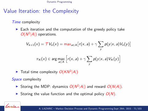
Value Iteration: the Complexity
Time complexityI Each iteration and the computation of the greedy policy take
O(N2|A|) operations.
Vk+1(x) = T Vk(x) = maxa∈A[r(x , a) + γ
∑y
p(y |x , a)Vk(y)]
πK (x) ∈ arg maxa∈A
[r(x , a) + γ
∑y
p(y |x , a)VK (y)]
I Total time complexity O(KN2|A|)
Space complexityI Storing the MDP: dynamics O(N2|A|) and reward O(N|A|).I Storing the value function and the optimal policy O(N).
A. LAZARIC – Markov Decision Process and Dynamic Programming Sept 29th, 2015 - 71/103

Dynamic Programming
State-Action Value Function
DefinitionIn discounted infinite horizon problems, for any policy π, thestate-action value function (or Q-function) Qπ : X × A 7→ R is
Qπ(x , a) = E[∑
t≥0γtr(xt , at)|x0 = x , a0 = a, at = π(xt), ∀t ≥ 1
],
and the corresponding optimal Q-function is
Q∗(x , a) = maxπ
Qπ(x , a).
A. LAZARIC – Markov Decision Process and Dynamic Programming Sept 29th, 2015 - 72/103

Dynamic Programming
State-Action Value Function
The relationships between the V-function and the Q-function are:
Qπ(x , a) = r(x , a) + γ∑y∈X
p(y |x , a)V π(y)
V π(x) = Qπ(x , π(x))
Q∗(x , a) = r(x , a) + γ∑y∈X
p(y |x , a)V ∗(y)
V ∗(x) = Q∗(x , π∗(x)) = maxa∈AQ∗(x , a).
A. LAZARIC – Markov Decision Process and Dynamic Programming Sept 29th, 2015 - 73/103
Dynamic Programming
Value Iteration: Extensions and Implementations
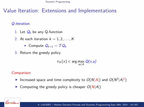
Q-iteration.
1. Let Q0 be any Q-function
2. At each iteration k = 1, 2, . . . ,KI Compute Qk+1 = T Qk
3. Return the greedy policy
πK (x) ∈ arg maxa∈A
Q(x,a)
ComparisonI Increased space and time complexity to O(N|A|) and O(N2|A|2)
I Computing the greedy policy is cheaper O(N|A|)
A. LAZARIC – Markov Decision Process and Dynamic Programming Sept 29th, 2015 - 74/103
Dynamic Programming
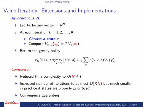
Value Iteration: Extensions and ImplementationsAsynchronous VI.
1. Let V0 be any vector in RN
2. At each iteration k = 1, 2, . . . ,KI Choose a state xkI Compute Vk+1(xk) = T Vk(xk)
3. Return the greedy policy
πK (x) ∈ arg maxa∈A
[r(x , a) + γ
∑y
p(y |x , a)VK (y)].
ComparisonI Reduced time complexity to O(N|A|)I Increased number of iterations to at most O(KN) but much smaller
in practice if states are properly prioritizedI Convergence guarantees
A. LAZARIC – Markov Decision Process and Dynamic Programming Sept 29th, 2015 - 75/103
Dynamic Programming
How to solve exactly an MDP
Dynamic Programming
Bellman Equations
Value Iteration
Policy Iteration
A. LAZARIC – Markov Decision Process and Dynamic Programming Sept 29th, 2015 - 76/103

Dynamic Programming
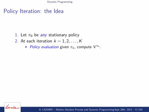
Policy Iteration: the Idea
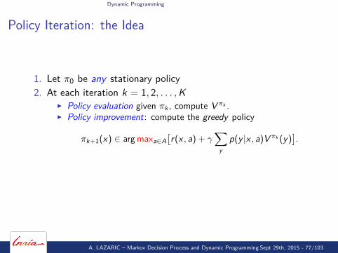
1. Let π0 be any stationary policy
2. At each iteration k = 1, 2, . . . ,KI Policy evaluation given πk , compute V πk .I Policy improvement: compute the greedy policy
πk+1(x) ∈ arg maxa∈A[r(x , a) + γ
∑y
p(y |x , a)V πk (y)].
3. Return the last policy πK
Remark: usually K is the smallest k such that V πk = V πk+1 .
A. LAZARIC – Markov Decision Process and Dynamic Programming Sept 29th, 2015 - 77/103

Dynamic Programming
Policy Iteration: the Idea
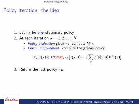
1. Let π0 be any stationary policy2. At each iteration k = 1, 2, . . . ,K
I Policy evaluation given πk , compute V πk .I Policy improvement: compute the greedy policy
πk+1(x) ∈ arg maxa∈A[r(x , a) + γ
∑y
p(y |x , a)V πk (y)].
3. Return the last policy πK
Remark: usually K is the smallest k such that V πk = V πk+1 .
A. LAZARIC – Markov Decision Process and Dynamic Programming Sept 29th, 2015 - 77/103
Dynamic Programming
Policy Iteration: the Idea
1. Let π0 be any stationary policy2. At each iteration k = 1, 2, . . . ,K
I Policy evaluation given πk , compute V πk .
I Policy improvement: compute the greedy policy
πk+1(x) ∈ arg maxa∈A[r(x , a) + γ
∑y
p(y |x , a)V πk (y)].
3. Return the last policy πK
Remark: usually K is the smallest k such that V πk = V πk+1 .
A. LAZARIC – Markov Decision Process and Dynamic Programming Sept 29th, 2015 - 77/103
Dynamic Programming
Policy Iteration: the Idea
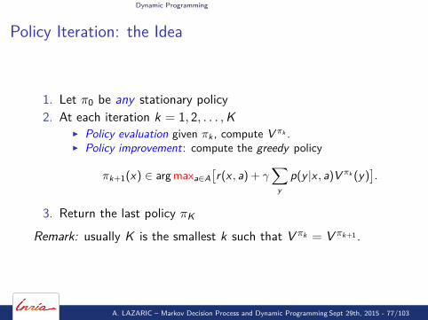
1. Let π0 be any stationary policy2. At each iteration k = 1, 2, . . . ,K
I Policy evaluation given πk , compute V πk .I Policy improvement: compute the greedy policy
πk+1(x) ∈ arg maxa∈A[r(x , a) + γ
∑y
p(y |x , a)V πk (y)].
3. Return the last policy πK
Remark: usually K is the smallest k such that V πk = V πk+1 .
A. LAZARIC – Markov Decision Process and Dynamic Programming Sept 29th, 2015 - 77/103
Dynamic Programming
Policy Iteration: the Idea
1. Let π0 be any stationary policy2. At each iteration k = 1, 2, . . . ,K
I Policy evaluation given πk , compute V πk .I Policy improvement: compute the greedy policy
πk+1(x) ∈ arg maxa∈A[r(x , a) + γ
∑y
p(y |x , a)V πk (y)].
3. Return the last policy πK
Remark: usually K is the smallest k such that V πk = V πk+1 .
A. LAZARIC – Markov Decision Process and Dynamic Programming Sept 29th, 2015 - 77/103
Dynamic Programming
Policy Iteration: the Guarantees
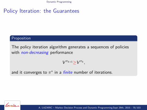
Proposition
The policy iteration algorithm generates a sequences of policieswith non-decreasing performance
V πk+1≥V πk ,
and it converges to π∗ in a finite number of iterations.
A. LAZARIC – Markov Decision Process and Dynamic Programming Sept 29th, 2015 - 78/103
Dynamic Programming
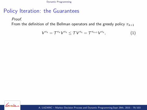
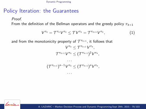
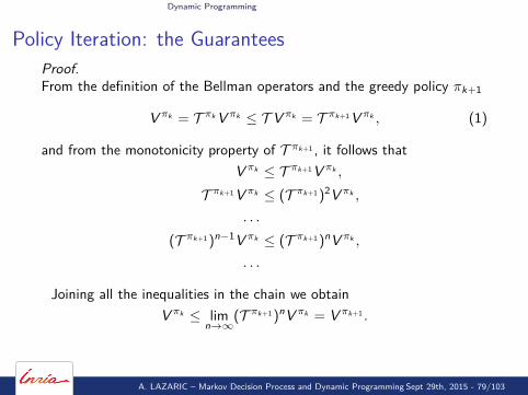
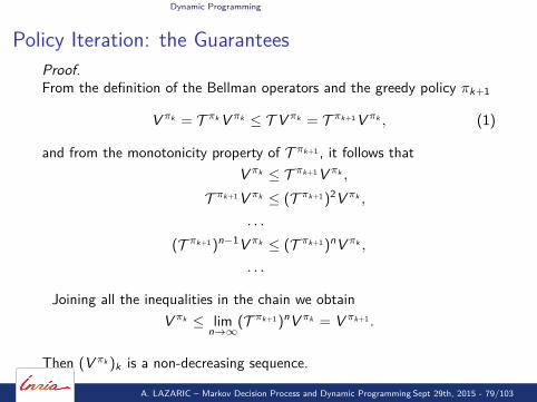
Policy Iteration: the GuaranteesProof.From the definition of the Bellman operators and the greedy policy πk+1
V πk = T πk V πk ≤ T V πk = T πk+1 V πk , (1)
and from the monotonicity property of T πk+1 , it follows thatV πk ≤ T πk+1 V πk ,
T πk+1 V πk ≤ (T πk+1 )2V πk ,
. . .
(T πk+1 )n−1V πk ≤ (T πk+1 )nV πk ,
. . .
Joining all the inequalities in the chain we obtainV πk ≤ lim
n→∞(T πk+1 )nV πk = V πk+1 .
Then (V πk )k is a non-decreasing sequence.
A. LAZARIC – Markov Decision Process and Dynamic Programming Sept 29th, 2015 - 79/103
Dynamic Programming
Policy Iteration: the Guarantees
Proof (cont’d).Since a finite MDP admits a finite number of policies, then thetermination condition is eventually met for a specific k.Thus eq. 2 holds with an equality and we obtain
V πk = T V πk
and V πk = V ∗ which implies that πk is an optimal policy. �
A. LAZARIC – Markov Decision Process and Dynamic Programming Sept 29th, 2015 - 80/103

Dynamic Programming
Policy Iteration
Notation. For any policy π the reward vector is rπ(x) = r(x , π(x))and the transition matrix is [Pπ]x ,y = p(y |x , π(x))
A. LAZARIC – Markov Decision Process and Dynamic Programming Sept 29th, 2015 - 81/103
Dynamic Programming
Policy Iteration: the Policy Evaluation StepI Direct computation. For any policy π compute
V π = (I − γPπ)−1rπ.
Complexity: O(N3) (improvable to O(N2.807)).
I Iterative policy evaluation. For any policy π
limn→∞
T πV0 = V π.
Complexity: An ε-approximation of V π requires O(N2 log 1/εlog 1/γ ) steps.
I Monte-Carlo simulation. In each state x , simulate n trajectories((x i
t )t≥0,)1≤i≤n following policy π and compute
V̂ π(x) ' 1n
n∑i=1
∑t≥0
γtr(x it , π(x i
t )).
Complexity: In each state, the approximation error is O(1/√
n).
A. LAZARIC – Markov Decision Process and Dynamic Programming Sept 29th, 2015 - 82/103
Dynamic Programming
Policy Iteration: the Policy Evaluation StepI Direct computation. For any policy π compute
V π = (I − γPπ)−1rπ.
Complexity: O(N3) (improvable to O(N2.807)).I Iterative policy evaluation. For any policy π
limn→∞
T πV0 = V π.
Complexity: An ε-approximation of V π requires O(N2 log 1/εlog 1/γ ) steps.
I Monte-Carlo simulation. In each state x , simulate n trajectories((x i
t )t≥0,)1≤i≤n following policy π and compute
V̂ π(x) ' 1n
n∑i=1
∑t≥0
γtr(x it , π(x i
t )).
Complexity: In each state, the approximation error is O(1/√
n).
A. LAZARIC – Markov Decision Process and Dynamic Programming Sept 29th, 2015 - 82/103

Dynamic Programming
Policy Iteration: the Policy Improvement Step
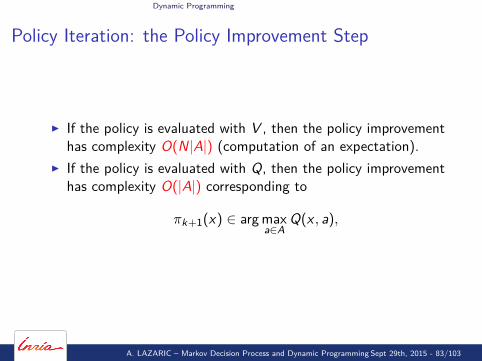
I If the policy is evaluated with V , then the policy improvementhas complexity O(N|A|) (computation of an expectation).
I If the policy is evaluated with Q, then the policy improvementhas complexity O(|A|) corresponding to
πk+1(x) ∈ arg maxa∈A
Q(x , a),
A. LAZARIC – Markov Decision Process and Dynamic Programming Sept 29th, 2015 - 83/103
Dynamic Programming
Policy Iteration: the Policy Improvement Step
I If the policy is evaluated with V , then the policy improvementhas complexity O(N|A|) (computation of an expectation).
I If the policy is evaluated with Q, then the policy improvementhas complexity O(|A|) corresponding to
πk+1(x) ∈ arg maxa∈A
Q(x , a),
A. LAZARIC – Markov Decision Process and Dynamic Programming Sept 29th, 2015 - 83/103
Dynamic Programming
Policy Iteration: Number of Iterations
I At most O(N|A|
1−γ log( 11−γ )
)
A. LAZARIC – Markov Decision Process and Dynamic Programming Sept 29th, 2015 - 84/103
Dynamic Programming
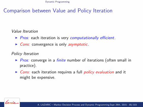
Comparison between Value and Policy Iteration
Value IterationI Pros: each iteration is very computationally efficient.I Cons: convergence is only asymptotic.
Policy IterationI Pros: converge in a finite number of iterations (often small in
practice).I Cons: each iteration requires a full policy evaluation and it
might be expensive.
A. LAZARIC – Markov Decision Process and Dynamic Programming Sept 29th, 2015 - 85/103
Dynamic Programming
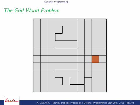
The Grid-World Problem
A. LAZARIC – Markov Decision Process and Dynamic Programming Sept 29th, 2015 - 86/103
Dynamic Programming
How to solve exactly an MDP
Dynamic Programming
Bellman Equations
Value Iteration
Policy Iteration
A. LAZARIC – Markov Decision Process and Dynamic Programming Sept 29th, 2015 - 87/103
Dynamic Programming
Other Algorithms
I Modified Policy IterationI λ-Policy IterationI Linear programmingI Policy search
A. LAZARIC – Markov Decision Process and Dynamic Programming Sept 29th, 2015 - 88/103
Dynamic Programming
Summary
I Bellman equations provide a compact formulation of valuefunctions
I DP provide a general tool to solve MDPs
A. LAZARIC – Markov Decision Process and Dynamic Programming Sept 29th, 2015 - 89/103
Dynamic Programming
Bibliography I
R. E. Bellman.Dynamic Programming.Princeton University Press, Princeton, N.J., 1957.
D.P. Bertsekas and J. Tsitsiklis.Neuro-Dynamic Programming.Athena Scientific, Belmont, MA, 1996.
W. Fleming and R. Rishel.Deterministic and stochastic optimal control.Applications of Mathematics, 1, Springer-Verlag, Berlin New York, 1975.
R. A. Howard.Dynamic Programming and Markov Processes.MIT Press, Cambridge, MA, 1960.
M.L. Puterman.Markov Decision Processes: Discrete Stochastic Dynamic Programming.John Wiley & Sons, Inc., New York, Etats-Unis, 1994.
A. LAZARIC – Markov Decision Process and Dynamic Programming Sept 29th, 2015 - 90/103