masarykoav univerzita p°írodov¥decák...

MASARYKOVA UNIVERZITAP°írodov¥decká fakulta

Ústav teoretické fyziky a astrofyziky

DIPLOMOVÁ PRÁCE

Studium mikrokvasar·

Ondrej Kamenský

�kolitel: Mgr. Filip Hroch, Ph.D.

2016

Bibliogra�cký záznam

Autor: Ondrej KamenskýP°írodov¥decká fakulta, Masarykova univerzitaÚstav teoretické fyziky a astrofyziky

Název práce: Studium mikrokvasar·

Studijní program: Fyzika

Studijní obor: Teoretická fyzika a astrofyzika

Vedoucí práce: Mrg. Filip Hroch, Ph.D.

Akademický rok: 2015/2016

Po£et stran: 69

Klí£ová slova: mikrokvasar, BHXB, £erná díra, akre£ní disk

Bibliogra�c Entry

Author: Ondrej KamenskýFaculty of Science, Masaryk UniversityDepartment of Theoretical Physicsand Astrophysics

Title of Thesis: Study of microquasars

Degree Programme: Physics

Field of Study: Theoretical physics and astrophysics

Supervisor: Mrg. Filip Hroch, Ph.D.

Academic Year: 2015/2016

Number of Pages: 69

Keywords: microquasar, BHXB, black hole, accretion disc

Abstrakt

Tato práce má dva cíle. Prvním cílem je poskytnout £tená°i základní informaceo mikrokvasarech a o postupech pro zpracování a analýzu dat. Druhým cílem jesamotné studium mikrokvasar· GX 339-4 a Cygnus X-1. První kapitoly se zabývajíteorií s podporou £lánk· pokrývajících dané téma. T°etí kapitola popisuje získávánía zpracování dat pro jednotlivé rentgenové mise. Poslední kapitoly jsou ur£enystudiu vybraných objekt·, shrnutí výsledk· a diskuzi.

Klí£ová slova: mikrokvasar, BHXB, £erná díra, akre£ní disk

Abstract

The aim of this work is to provide a reader with basic information on microquasarsand on data reduction and analysis procedures. Another aim is a study of micro-quasars GX 339-4 and Cygnus X-1. First chapters deal with theory referencingmost recent articles covering this topic. Chapter three describes data retrieval andreduction processes for individual X-ray missions. The last chapters are dedicatedto the study of the microquasars, results summary and a discussion of the results.

Keywords: microquasar, BHXB, black hole, accretion disc

I would like to thank my supervisor for having enough belief in me, that he did notpush me and rush me, knowing that I would deliver the thesis in time. I would liketo thank him for his advices and remarks. I also would like to thank my girlfriendfor her support, for keeping me optimistic and for her understanding in all the timeswhen this work had to be prioritised instead of her.

I declare that I wrote my thesis independently and exclusively with the use of ref-erences cited. I agree to lending and publishing of the thesis.

Brno, 10.5.2016 Ondrej Kamenský

Contents

Acronyms 9

Introduction 10

1 Microquasars 11

1.1 Accretion as a source of energy . . . . . . . . . . . . . . . . . . . . . 121.2 Known objects and parameters . . . . . . . . . . . . . . . . . . . . . 14

1.2.1 Mass function . . . . . . . . . . . . . . . . . . . . . . . . . . . 151.3 Quantitative description . . . . . . . . . . . . . . . . . . . . . . . . . 15

1.3.1 X-ray states in spectra . . . . . . . . . . . . . . . . . . . . . . 181.4 Qualitative description . . . . . . . . . . . . . . . . . . . . . . . . . . 19

1.4.1 Thermal component . . . . . . . . . . . . . . . . . . . . . . . 191.4.2 Power law component . . . . . . . . . . . . . . . . . . . . . . 241.4.3 Re�ection component . . . . . . . . . . . . . . . . . . . . . . 251.4.4 Fe-Kα line component . . . . . . . . . . . . . . . . . . . . . . 251.4.5 Absorption component . . . . . . . . . . . . . . . . . . . . . . 26

2 Objects of interest 27

2.1 GX 339-4 . . . . . . . . . . . . . . . . . . . . . . . . . . . . . . . . . 272.2 Cyg X-1 . . . . . . . . . . . . . . . . . . . . . . . . . . . . . . . . . . 28

3 Detectors 29

3.1 Suzaku . . . . . . . . . . . . . . . . . . . . . . . . . . . . . . . . . . . 293.1.1 Data retrieval . . . . . . . . . . . . . . . . . . . . . . . . . . . 303.1.2 Spectrum extraction . . . . . . . . . . . . . . . . . . . . . . . 30

3.2 XMM Newton . . . . . . . . . . . . . . . . . . . . . . . . . . . . . . . 323.2.1 Data retrieval . . . . . . . . . . . . . . . . . . . . . . . . . . . 343.2.2 Spectrum extraction . . . . . . . . . . . . . . . . . . . . . . . 34

4 Data retrieval and reduction 36

4.1 GX 339-4 . . . . . . . . . . . . . . . . . . . . . . . . . . . . . . . . . 364.1.1 XMM Newton . . . . . . . . . . . . . . . . . . . . . . . . . . 364.1.2 Suzaku . . . . . . . . . . . . . . . . . . . . . . . . . . . . . . . 37

4.2 Cyg X-1 . . . . . . . . . . . . . . . . . . . . . . . . . . . . . . . . . . 38

7

4.2.1 XMM Newton . . . . . . . . . . . . . . . . . . . . . . . . . . 384.2.2 Suzaku . . . . . . . . . . . . . . . . . . . . . . . . . . . . . . . 39

5 GX 339-4 40

5.1 Fitting re�ection . . . . . . . . . . . . . . . . . . . . . . . . . . . . . 425.2 BHSPEC �tting . . . . . . . . . . . . . . . . . . . . . . . . . . . . . . 44

6 Cyg X-1 49

6.1 Fitting re�ection . . . . . . . . . . . . . . . . . . . . . . . . . . . . . 516.2 BHSPEC �tting . . . . . . . . . . . . . . . . . . . . . . . . . . . . . . 53

7 Results 60

8 Discussion 62

References 63

Electronic references and sources 67

Appendix A - Spectrum extraction 68

8

Acronyms

This is a list of acronyms used in this thesis. They are commonly used in this �eldof study and should ease the reading of the work.

Acronym De�nitionAGN Active Galactic NucleiBH Black HoleBHC Black Hole CandidateBHXB Black Hole X-ray BinaryHID Hardness Intensity DiagramHMXB High Mass X-ray BinaryHR Hardness RatioISCO Inner-most Stable Circular OrbitLMXB Low Mass X-ray BinaryLOS Line Of SightMBB MultiBlackBodyMQ MicroquasarNS Neutron StarNSXB Neutron Star X-ray BinaryPL Power LawSPL Steep Power LawSSD Shakura-Sunyaev Disk

9

Introduction

All history of science provides many examples of astrophysics in�uencing theoreticalphysics. The Newton's gravitation and the theory of general relativity are examples.A problem theoretical physics is facing, concerning black hole (BH) physics, is a lackof experiments, a lack of actual BHs somebody can work with. Therefore, astro-physical BHs are the only objects available for testing BH theories. Microquasars(MQs) provide us with a chance to study BH physics, accretion processes, highenergy physics and a chance to test other theories otherwise unprovable. Studies ofMQs have gone through much development and even though archives are plentifulwith data, many of the processes are not properly understood yet. Despite years ofresearch, only a handful of properties and parameters have been determined withsuch certainty that they are recognised as correct. Unfortunately, most of the resultsare still just estimates and need to be re-approached, need to be tested in variousways in order to be proven correct. The aim of this work is to present MQs, to de-scribe the variability they undergo, to demonstrate ways of studying them and totest some of the recent results or to bring new ones.

Figure 2: A microquasar � an artist's impression [e1]

10

Chapter 1

Microquasars

�What the hell is a (micro)quasar?�

(Arnold J. Rimmer)

A (MQ) is a label for a black hole X-ray binary (BHXB). The �rst object tobe referred to as MQ is 1E170.7-2942 due to a double sided jet detected comingfrom it. It was mimicking jets of a quasar, just on smaller scales. Therefore thename. Next objects to be called MQs were, for example, GRS1915+105 and SS433.However, not all BHXBs were labelled as MQs. The condition was the detectionof relativistic jets with bulk motion speed over 90 % of the speed of light. Thisnicely ruled out neutron star X-ray binaries (NSXBs), whose bulk motion speedswere measured to be below 50 % of the speed of light. However, a discovery ofhighly relativistic jet bursting from a NSXB broke the labelling rule. The jets losttheir role in determining a MQ.

Despite the scale di�erence between actual quasars and MQs, the processes driv-ing the activity of both classes might be quite similar. Of course the size di�erenceis related to the temporal variability and therefore jets are a reoccurring featureof a BHXB. This fact o�ers an idea that di�erent kinds of quasars might not becaused just by the point of view from which we observe the object. The reasonsfor di�erent behaviour might be more complicated, like di�erent morphology of thecentral surroundings or even state transitions on a very long time scale. Therefore,the terms BHXB and MQ become equal and shall be used interchangeably in therest of the work.

A MQ system consists of two main components, a donor star and a compactobject. The matter �owing from the donor star does not fall directly onto the com-pact object, but creates an accretion disc due to conservation of angular momentum.Other components are, for example, a corona as a source of high energy radiationand double-sided jets emitting radio radiation. The research of these objects isclosely connected to the development of the observational technology. New mis-sions bring new data, better than before. This kind of objects can be studied acrossa wide range of energies. Jets in radio wavelengths, companion star in visible light(only limited amount of cases) but most of all in higher energies, in X-ray wave-lengths. This thesis is focused on observing the X-ray radiation detected with X-rayspacecrafts orbiting Earth.

11

Figure 1.1: A description of the components of a MQ system (Fender, 2002)

1.1 Accretion as a source of energy

We will consider the amount of energy extracted from nuclear fusion reactions.The highest e�ciency is reached in the case of hydrogen atoms being merged intohelium, which is also the most common case of such a reaction in stars. The amountof energy is

∆E = 0.007mc2, (1.1)

wherem stands for the mass of the hydrogen entering the reaction and c is the speedof light (Frank et al., 2002). This process extracts ∼ 4×1030 keV.kg−1. To comparenuclear fusion to accretion, we will set a simple approximation of spherically sym-metric inward fall of material onto a compact object. The extracted gravitationalenergy will be

∆E =GM∗m

R∗. (1.2)

In the case of an accreting neutron star with radius R∗ ∼ 10 km and M∗ ∼ M�the e�ciency results in ∼ 6×1031 keV.kg−1, being about 15 times higher thanin the case of nuclear hydrogen burning. Nevertheless, this e�ciency is a functionof �compactness� of the central object. As the ratioM∗/R∗ gets higher, the e�ciencygets higher as well.

12

However, this is a rather simple approximation of matter falling directly inwards.In reality, the matter is carrying non-zero angular momentum, which results inaccretion. The matter is accumulated in an accretion disk, following Keplerianvelocity distribution, v(r) ∝ r−1/2. This means that neighbouring areas of thematter have di�erent orbital velocities and slide past one another which, thanksto viscosity, creates shearing. This process helps to transfer angular momentumoutwards.

The inner parts of the disc moving with higher velocity need to eliminate the an-gular momentum in order to fall closer to the centre. This is achieved by shearing,when friction between two neighbouring areas allow for the angular momentum tobe transferred. The e�ciency of redistributing of the angular momentum dependson the viscosity of the material.

When falling inwards, part of the potential energy is transferred into kineticenergy. Another part is transferred into internal energy and heats up the matter.As the matter gets closer to the centre, the temperature rises. This results instrong thermal electromagnetic radiation from the disc itself. For a typical BHXB,the inner temperature of the disc rises up to ∼ 107 K, with the maximum of theradiation around X-ray wavelengths ∼ 0.25 nm. This emission plays an importantrole in studying MQs. (See Section 1.4.1)

Another important e�ect originating in the accretion process is the Eddingtonlimit. The mechanism of accretion brings the material closer and thus deliversfuel. However, outgoing radiation produces pressure upon the incoming material.As more material is delivered closer to the center, the luminosity rises and so does theradiation pressure. At a certain point, the radiation pressure may get so high thatit actually stops the inward �ow of the accreted material. This process results in theloss of fuel and luminosity decreases, along with the radiation pressure. Therefore,these objects cannot have higher luminosity than the Eddington limit for a long timeand if they ever reach the limit, they tend to �uctuate around it. To determine thelimit, we will set the radiation force equal to the gravitational force:

FL ≡LσT

4πr2c= Fg ≡

GMm

r2, (1.3)

where L is the luminosity, σT is the Thomson cross section, which is dependenton the material and m is the mass of the accreted particle. We can now express Lfor the case of fully ionized hydrogen with the mass of the central object expressedin solar masses:

LEdd =4πcGMm

σT= 1.26× 1031

(M

M�

)W. (1.4)

The accreted matter can be supplied from the companion star in two ways.In order to be trapped by the gravitational pull of the compact object the matter hasto leave the vicinity of the donor star, where it still �belongs� to the donor star. Thisis done either by a stellar wind or by the Roche lobe over�ow. The former situation is

13

less important, as stellar winds do not continuously supply a lot of matter to the disc.However, at some point of the evolution, a massive ejection of the mass mightoccur. The latter situation is either a result of the evolution of the star or a resultof a change in the binary orbital parameter. When momentum is lost (e.g. due tomass loss by stellar winds) the binary separation shrinks and the Roche lobe radiusis lowered. Most common cause of a star �lling its Roche lobe is the stellar evolution.The donor star can, in later phases of its evolution, blow away its upper atmosphereinto higher radii. At this point, the matter is moved from one gravitational wellto that of the compact object where it is accumulated in the accretion disc. In thecase of a high mass over�ow the stream can be a distinctive part of the system. Itcan, for example, cross the line of sight in short-period binaries and create variableabsorption.

1.2 Known objects and parameters

Table 1 provides a summary of MQs and their parameters taken from (Zhang,2013), combined with the spectral types of donor stars listed in the original tablefrom (Remillard and McClintock, 2006).

Coordinate Common Porb f(M) MBH Spec. type a∗Name Name/Pre�x (hr) (M�) (M�) (Donor) (cJ/GM2)

0422+32 (GRO J) 5.1 1.19±0.02 3.7�5.0 M2V �0620-003 (A) 7.8 2.72±0.06 6.35�6.85 K4V 0.12±0.191009-45 (GRS) 6.8 3.17±0.12 3.6�4.7 K7/M0V �1118+408 (XTE J) 4.1 6.10±0.30 6.5�7.2 K5/M0V �1124-684 Nova Mus 91 10.4 3.01±0.15 6.5�8.2 K3/K5V �1354-64 (GS) 61.1 5.75±0.30 � GIV �1543-475 4U 26.8 0.25±0.01 8.4�10.4 A2V 0.75�0.851550-564 (XTE J) 37.0 6.86±0.71 8.4�10.8 G8/K8IV 0.06�0.541650-500 (XTE J) 7.7 2.73±0.56 � K4V �1655-40 (GRO J) 62.9 2.73±0.09 6.0�6.6 F3/F5IV 0.65�0.751659-487 GX 339-4 42.1 5.80±0.50 � � �1705-250 Nova Oph 77 12.5 4.86±0.13 5.6�8.3 K3/7V �1743-322 (H) � � � � 0.20±0.301819.3-2525 V4641 Sgr 67.6 3.13±0.13 6.8�7.4 B9III �1859+226 (XTE J) 9.2 7.40±1.10 7.6�12.0 � �1915+105 (GRS) 804.0 9.80±3.00 10.0�18.0 K/MIII 0.98�1.01956+350 Cyg X-1 134.4 0.244±0.005 13.8�15.8 O9.7Iab > 0.952000+251 (GS) 8.3 5.01±0.12 7.1�7.8 K3/K7V �2023+338 V404 Cyg 155.3 6.08±0.06 10.0�13.4 K0III �

0538-641 LMC X-3 40.9 2.3±0.3 5.9�9.2 B3V < 0.30540-697 LMX X-1 93.8 0.13±0.05 9.4�12.5 O7III 0.94�0.99

0020+593 IC 10 X-1 34.9 7.64±1.26 > 20 � �0055-377 NGC 300 X-1 32.3 2.6±0.3 > 10 � �0133+305 M33 X-7 82.9 0.46±0.07 14.2�17.1 � 0.84±0.05

Table 1.1: Table of known MQs (Remillard and McClintock, 2006; Zhang, 2013)

14

1.2.1 Mass function

The values in the fourth column are the best estimates for the lower mass limitof the compact object. These results come from dynamical studies and thereforeare most reliable for the mass estimation. The �nal formula (1.9) is derived fromthe third Kepler law (1.5). Given that q ≡ M2/M1, the total mass of the systemcan be transformed (1.6) along with the major semiaxis (1.7). The inclination isdenoted as i. The major key of this procedure is the measurement of the orbitalperiod Porb and the radial velocity amplitude K2 of the donor star.

GM =

(2π

Porb

)2

a3, (1.5)

M = M1 +M2 = M1

(1 +

M2

M1

)= M1(1 + q), (1.6)

a3 = (a1 + a2)3 = a32(1 + q)3, (1.7)

Porb =2π

ω=

2πa2

v2=

2πa2 sin(i)

K2. (1.8)

All these combined give the following mass function f(M) (1.9). If the orbitalperiod and the radial velocity amplitude are measured, the mass function givesa lower mass limit of the compact source. The maximum value of sin i is 1 andthe minimal value of q is 0, making the f(M) the lower boundary forM1. Measuringthe mass function is a strong proof for deciding on whether a BHC is a true BH.

f(M) ≡ PorbK32

2πG=M1 sin3(i)

(1 + q)2(1.9)

1.3 Quantitative description

A discrete classi�cation of this kind of objects is very di�cult. Although signi�cantresults have been achieved for describing evolution tracks of BHXBs, di�erent ob-jects usually resemble each other only in basic traits due to di�erent conditions. Avery good, yet not absolutely complete tool, is a hardness intensity diagram (HID).The HID is an equivalent of the Hertzprung-Russel diagram for evolution tracking.However, the evolution in this case is in a form of a loop. The diagram depicts thesource intensity versus the hardness ratio (HR), computed as the ratio of count ratesin two energy bands. The big advantage of the HID is that it is model independent.An example of this diagram is shown in Figure 1.2.

We will set the right-bottom corner of the HID as the starting point of theevolution loop. This area of the �q-shaped� diagram is referred to as the quiescentstate. MQs tend to spend most of their lifetime in this state with low luminosity,high HR and very little variability. However, there are exceptions when a MQ doesnot fall into the quiescent state and rather immediately repeats the cycle.

15

One example of such behaviour is the GX 339-4 MQ, which has been veryactive since its discovery. On the other hand, the GRS1915+105 truly stays mostof the time (even years) in the calm, invariable quiescent state. Most of all, MQsare never discovered while in this state due to very faint luminosity. They aremostly discovered in the moment of an outburst and only then they can be trackedreturning into this stop of the cycle. In this state, the inner regions of the disc aretruncated, there is a sparse corona responsible for a weak hard X-ray component.Radio jets are weak and present rather randomly. The low luminosity of this stateis important for dynamical observations, as the spectrum of the donor star can getprominent and allow the measurement of orbit velocities.

Figure 1.2: Hardness Intensity Diagram (Motta et al., 2011)

In the case of an outburst the luminosity rises severely, with the HR remaininghigh. Previously random and weak jets are now strong and permanent. This verti-cal rise of the MQ is referred to as the hard state. At this point, the soft spectralcomponent is weak or even absent and a massive corona is formed, which resultsin a very strong hard power law component (PL) of the spectrum. The photonindex Γ of the PL is close to 1.7 and these spectra usually su�er from an exponen-tial cuto� near 100 keV. In addition, part of the hard X-ray radiation is scatteredtowards the disc and re�ected from it. Depending on the inclination of the disc in re-spect to the observer a re�ection component occurs along with possible occurrenceof the emission iron line feature.

16

The following state is the steep power law state (SPL). While in the hardstate the photon index was Γ ∼ 1.7, it rises above 2.4 in the SPL state. This stateis situated in the top left half of the HID. The inner regions of the disc are no moretruncated and the soft X-ray component of the spectrum is cognizable. Nonetheless,strong corona is still present and the hard X-ray component does not su�er fromthe cuto� and extends up to ∼MeV. Jets are present only till a certain breakpoint.When moving from right to left, the jet outburst may get violent when the MQ ispassing the middle section and disappear as the MQ gets closer to the left edge ofthe HID.

If we consider a simple case when the MQ undergoing an outburst directlyfollows the q-shaped loop, the MQ goes from the SPL state to the thermal (orsoft) state. This state has a distinctive thermal component described as ∼1 keVand a faint variable PL component. The weak PL component is due to absent orvery sparse corona and jets are not observed. As a result of the absence of a strongPL component, the re�ection component tends to be absent as well.

As stated at the beginning of the section, the previous discrete classi�cation isnot complete. There are numerous intermediate states, when a MQ transfers fromone state to the next one and shares features of both states. Especially the transitbetween the hard and the SPL state is very important as it correlates to the changesin the radio emissions and the restoration of the inner disc regions.

The truncation and re�lling of the inner regions of the accretion disc are con-nected to the spin parameter of the central BH. The spin is de�ned as a unitlessvalue a∗ ≡ cJ/GM2, where J is the angular momentum of the BH. The spin de-termines the innermost stable circular orbit (ISCO) of the disc. For non-rotatingSchwarzschild BHs with a∗ = 0 the ISCO lies at 6 rg. The opposite situationis a maximally rotating Kerr BH, with a∗ = 1, when the ISCO stretches downto 1 rg. (Remillard and McClintock, 2006) The gravitational radius is de�nedas rg ≡ GM/c2.

State name Features of X-ray state

Thermal Disk fraction fa > 75 %Tin ∼1 keVjets absent

Hard fa < 20 %1.4 < Γ < 2.1jets present∼100 keV cuto�

Steep Power Law (SPL) Γ > 2.4fa < 50 % - 80 %jets violent or absentPL up to ∼MeV

Table 1.2: Summary of the features of the MQ states. a is taken from (Remillardand McClintock, 2006).

17

1.3.1 X-ray states in spectra

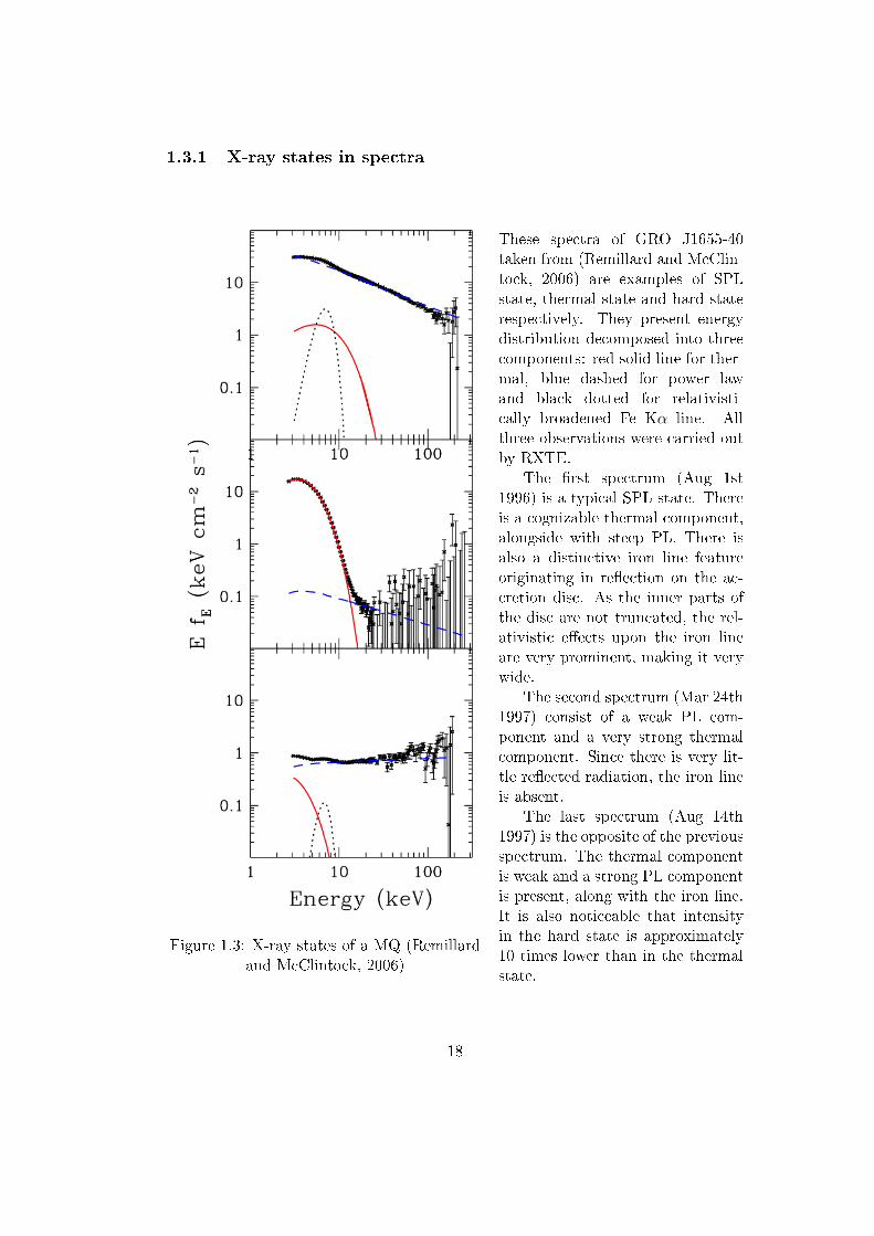
Figure 1.3: X-ray states of a MQ (Remillardand McClintock, 2006)

These spectra of GRO J1655-40taken from (Remillard and McClin-tock, 2006) are examples of SPLstate, thermal state and hard staterespectively. They present energydistribution decomposed into threecomponents: red solid line for ther-mal, blue dashed for power lawand black dotted for relativisti-cally broadened Fe Kα line. Allthree observations were carried outby RXTE.

The �rst spectrum (Aug 1st1996) is a typical SPL state. Thereis a cognizable thermal component,alongside with steep PL. There isalso a distinctive iron line featureoriginating in re�ection on the ac-cretion disc. As the inner parts ofthe disc are not truncated, the rel-ativistic e�ects upon the iron lineare very prominent, making it verywide.

The second spectrum (Mar 24th1997) consist of a weak PL com-ponent and a very strong thermalcomponent. Since there is very lit-tle re�ected radiation, the iron lineis absent.

The last spectrum (Aug 14th1997) is the opposite of the previousspectrum. The thermal componentis weak and a strong PL componentis present, along with the iron line.It is also noticeable that intensityin the hard state is approximately10 times lower than in the thermalstate.

18

1.4 Qualitative description

This section deals with the spectral components separately. It describes processesthat generate and shape particular components, mainly the thermal componentthat originates in the accretion disc itself. Most of all, it presents commonly usedXSPEC (Arnaud, 1996) models designed for each of the components, describes theirparameters and in some cases compares di�erent XSPEC models.

1.4.1 Thermal component

Thin disc prescription

A thin disk model is an approximation neglecting the thickness of the disc in thecylindrical coordinate system. It provides reasonable results for cases when H �R, where H is the horizontal thickness of the disc. Fortunately, this conditionis often met. One example of such model is the Sakura-Sunyaev (SSD) thin discsolution (Frank et al., 2002). The model includes a unitless parameter α, whichrepresents a certain law of viscosity of the accreted material as ν = αcsH where cs

is the sound velocity. This parameter is usually given beforehand to be 0.1 or 0.01and is almost never estimated by �tting. These equations were taken from (Franket al., 2002) (expressed in cgs system) and describe some of the disc parameters:

Σ = ρH, (1.10)

Tc = 1.4× 104α−1/5M3/1016 m

1/41 R

−3/410 f5/6K, (1.11)

Σ = 5.2× α−4/5M7/1010 m

1/41 R

−3/410 f14/5g.cm−2, (1.12)

H = 1.7× 108α−1/10M3/2016 m

−3/81 R

9/810 f

3/5cm, (1.13)

ν = 1.8× 1014α4/5M3/1016 m

−1/41 R

3/410 f

6/5cm2.s−1, (1.14)

vR = 2.7× 104α4/5M3/1016 m

−1/41 R

−1/410 f−14/5cm.s−1, (1.15)

f =

[1−

(R∗R

)1/2]1/4

, (1.16)

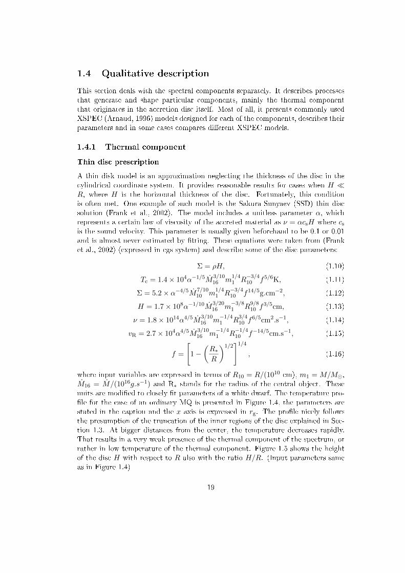
where input variables are expressed in terms of R10 = R/(1010 cm), m1 = M/M�,M16 = M/(1016g.s−1) and R∗ stands for the radius of the central object. Theseunits are modi�ed to closely �t parameters of a white dwarf. The temperature pro-�le for the case of an ordinary MQ is presented in Figure 1.4, the parameters arestated in the caption and the x axis is expressed in rg. The pro�le nicely followsthe presumption of the truncation of the inner regions of the disc explained in Sec-tion 1.3. At bigger distances from the center, the temperature decreases rapidly.That results in a very weak presence of the thermal component of the spectrum, orrather in low temperature of the thermal component. Figure 1.5 shows the heightof the disc H with respect to R also with the ratio H/R. (Input parameters sameas in Figure 1.4)

19

Figure 1.4: SSD temperature pro�le (M = 15.0 M�, α = 0.1, M = 10−6 M�.y−1)

Figure 1.5: Height of the disc H and ratio H/R as functions of radius R.

20

Multi blackbody

Describing radiation from a disc with a temperature pro�le as shown in Figure 1.4by a simple blackbody model would be incorrect, since there is no constant temper-ature. However, there is a distinctive �inner� temperature, the highest temperatureat the inner boundary. The rest of the pro�le follows a rather simple function closeto ∼ R−3/4. The overall spectrum can thus be described as a multi-blackbody spec-trum (MBB). This spectrum can be acquired by integrating multiple blackbodydistributions over the disc temperature pro�le:

f(E) =cos θ

D2

∫ rout

rin

2πrB(E, T )dr =

=8πr2

in cos θ

3D2

∫ Tin

Tout

(T

Tin

)−11/3

B(E, T )dT

Tin,

(1.17)

where D stands for distance, θ stands for disc inclination, Tin = T (rin) is the high-est temperature at the inner edge of the disc and B(E, T ) represents the Planckblackbody distribution. (Mitsuda et al., 1984) The result of this simple MBB modelis presented in Figure 1.6, using the temperature pro�le in Figure 1.4. As well asstars cannot be precisely described as black bodies, describing an accretion disc bya multi black body pro�le is not entirely correct. Nonetheless, it provides a ratheraccurate estimate.

Figure 1.6: MBB pro�le, result of Equation (1.17) applied to Figure 1.4

21

DISKBB and BHSPEC

DISKBB is a basic model in XSPEC and represents a simple MBB model similarto SSD. It has two input parameters, Tin and norm. Tin is the inner temperatureand corresponds to the temperature in (1.17). The parameter norm represents[

(Rin/km)

(D/10kpc)

]2

cos θ, (1.18)

where Rin is the inner disc radius, D is the distance and θ is the disc inclination.An example of DISKBB is included in Figure 1.7, where the shape of the thermalcomponent resembles the pro�le in Figure 1.6 rather well.

BHSPEC computes the thermal spectrum of an accretion disc with respect to rel-ativistic e�ects (Davis et al., 2005). It uses models of stellar atmospheres to calculatethe radiation from disc annuli. The model is in a tabular form and user has to choosea particular table based for example on the α parameter. The relativistic e�ects arementioned in the paragraph about the iron line component.

The input parameters of the BHSPEC are the logarithmic mass of the compactobject log(M/M�), the logarithmic luminosity of the MQ as a fraction of the Ed-dington luminosity log(L/Ledd), the cosine of the inclination of the disc cos i, theunitless spin parameter of the compact object a∗ and the normalisation parameternorm = (10kpc/D)2, where D stands for distance.

Figure 1.7: BHXB modelled spectrum components (Paizis et al., 2009)

22

Figure 1.8 compares the two XSPEC models BHSPEC and DISKBB. First, sim-ulated data were generated using models wabs*bhspec. The model WABS repre-sents interstellar absorption and is dealt with in Section 1.4.5. The input parameterswere nH = 0.526, log(M/M�) = 1.14, log(L/Ledd) = −1.04, cos i = 0.7, a∗ = 0.98,norm = 9.0 and data were generated using response matrices of PN instrumentof XMM Newton from the observation number 0148220201 (GX 339-4). Afterwards,the simulated data were �tted with wabs*diskbb in order to demonstrate the dif-ferences. The resulting parameters of the DISKBB model were Tin = 0.876 keV andnorm = 9228.61.

If the K and cos i parameters are inserted into the DISKBB's norm parameter,the inner radius results in Rin ≈ 38 km. As a∗ approaches 1, the ISCO falls downto 1 rg. In this situation the spin parameter was �xed at near maximum valuea∗ = 0.98 and Rin is above the rg which is ∼ 20.5 km.

The bottom part of Figure 1.8 contains ratio between the simulated data and themodel. Even though the di�erences might seem su�ciently large, the probability ofthem being detected depends on the quality of the studied data. The choice whichmodel to use should be a�ected by presumption of the inner radius. When the innerregions of the disc are truncated, the relativistic e�ects are not very prominent anda simple model is su�cient. However, when considering SPL or Thermal state,the disc extends down to low radii and the relativistic e�ects may strongly in�uencethe radiation.

0.1

1

10

ke

V (

Ph

oto

ns c

m−

2 s

−1 k

eV

−1)

1 2 5

1

1.2

1.4

1.6

ratio

Energy (keV)

Figure 1.8: DISKBB applied to simulated BHSPEC data and model to data ratio

23

1.4.2 Power law component

This component is expressed by a quite simple formula (1.19) but the mechanismbehind this high energy radiation is still a bit unclear. The mostly accepted theoryuses inverse Compton scattering to produce the non-thermal radiation.

A(E) = K.E−Γ (1.19)

The scattering is thought to occur in a corona, consisting of very hot electrons. Thecorona is created by evaporation of the accreted material in the inner regions of thedisc. Thermal photons coming from the disc are scattered up by the electrons tohigher energies. While the disc occupies regions outside rin, the corona is locatedbetween rin and ISCO. In the hard state rin � ISCO and thus the disc emissionis poor and sometimes hardly detectable. Otherwise, in the soft state rin → ISCOand the corona is absent while the disc dominates the spectrum.

In XSPEC, two basic models represent this spectral component, POWERLAWand BKNPOWER. The POWERLAW model has two input parameters, the photonindex Γ and the multiplication factor K (photons keV−1cm−2s−1 at 1 keV). An ex-ample of POWERLAW is contained in Figure 1.9 (red dotted line). The BKN-POWER model has a broken power law pro�le. It has four parameters: two photonindexes Γ1 and Γ2, normalisation K parameter and a break point for the energyEbreak. The broken power law model is applicable to a spectrum that su�ers frominconsistency, for example in the case of inconsistent temperature pro�le.

Figure 1.9: Spectral components (Adapted from Figure 3b from (Miller, 2007))

24

1.4.3 Re�ection component

A typical feature of this component is a Comptonian hump with a maximumat ∼20 keV and an emission Fe Kα line as seen in Figure 1.9 (green dashed line).The re�ection models use an ordinary power law distribution of radiation to simu-late the re�ected spectrum. Most models work with an optically-thick disc and solveradiative transfer equations to obtain the outgoing radiation. As for the XSPECmodels, this work uses RELXILL model (García et al., 2013), which is a resultof merging XILLVER (continuum re�ection), RELLINE (relativistically broadenedemission lines) and RELCONV (relativistic smearing of the whole spectrum).

The RELXILL model is a table model with 15 parameters, of which many arefrozen by default. To name a few of the parameters, the model �ts for the ironabundance of the disc, the ionization parameter χi, the photon index of the powerlaw illumination Γ, rin, rout, inclination, spin of the BH and more.

1.4.4 Fe-Kα line component

The re�ection of high energy radiation on the accretion disc results in occurrenceof a �uorescent iron Kα line at 6.4 keV. This spectral component is very importantbecause it allows probing the inner parts of the disc without the need of knowing theexact distance of an object in contrary with the continuum �tting method. The rel-ativistic e�ects acting upon the line pro�le are dependent for example on the radiusand thus the line can be used to derive the rin parameter and to estimate the spinof a BH.

The relativistic e�ects are presented in Figure 1.10. A simple emission line isthermally broadened and then two e�ects are applied: gravitational redshift (1.20)and relativistic boosting (1.21). The redshift was taken and simpli�ed from (Baoet al., 1994). Figure 1.10 shows the asymmetric line broadening for di�erent incli-nation angles.

z =

(r

r − 3

)1/2

+

(r

(r − 2) (r − 3)

)1/2

sin isinφs√

1− cos2 φs sin2 i− 1, (1.20)

I =

(ω

ω0

)3

I0. (1.21)

In (1.20) r stands for the radius of currently processed segment, φs is its azimuth(the observer is at φs = 0) and i is the system inclination. In the process of creatingthe spectrum in Figure 1.10, the disc was divided into a set of annuli divided intoangular segments. An emission line was calculated for each segment and thermalDoppler broadening was used. (temperature and density derived from parametersin Figure 1.4) Then for each segment, both relativistic e�ects were applied. Theresult is of course just a rough example, supposed to present the relativistic e�ects.It does not include variable disc emissivity or any iron abundance pro�le.

25

Figure 1.10: Relativistic broadening of an emission line

In XSPEC, the Fe Kα line is included in some re�ection models, but can beapplied separately. The models are LAOR and KYRLINE. Description and com-parison of these two models can be found in (Svoboda et al., 2009).

1.4.5 Absorption component

The contribution to this process can be split between two sources, the interstellarabsorption and the absorption occurring within the MQ. The former tends to remainconstant, while the latter tends to change. As for X-ray radiation, absorption a�ectsmostly soft X-rays (thermal component) and should never be omitted from the�tting procedure. In XSPEC, there are many default models for the absorption,e.g. WABS, PHABS, TBABS, etc. Di�erences between models are caused by whatprocesses the model takes into account. A physical parameter all of them share isthe hydrogen column density nH (1022 atoms/cm2). As for X-ray wavelengths theabsorption is not at all dominated by hydrogen atoms, but by heavier elements.Their relative abundances are expressed by the hydrogen column.

When working with X-ray spectra, it is advisable to set boundaries of the nHparameter. These boundaries can be looked for in other articles concerning the ob-jects of interest or derived from HI surveys from the area. And while the interstellarcomponent is usually constant, the other component may vary on di�erent scales.The MQ Cyg X-1, for example, has been reported to show strong nH variabilityover its 5.6 days binary orbit period. (Grinberg et al., 2015)

26

Chapter 2

Objects of interest

2.1 GX 339-4

This MQ was discovered in 1973 (Markert et al., 1973) and is classi�ed as a LowMass X-ray Binary. The low mass de�nition describes the companion star, whosemass is comparable to the mass of the Sun. It is located in the constellation Ara atcoordinates α = 17◦02'49.36� and δ = -48◦47'22.8�. Due to the fact that GX 339-4is very active and has undergone many outbursts the spectral class of the companionstar is uncertain. GX 339-4 does not fall into the quiescent state and rather tends torepeat the outburst cycle without its brightness lowering very much. An importantpoint in the research of this object is the determination of the mass function withdynamical methods from spectroscopic data (Hynes et al., 2003). The mass functionexplained in Section 1.2 is in the case of GX 339-4 estimated to be (5.8±0.5) M�and the mass ratio q ≤ 0.08. Inserting these two values in Equation (1.9) allowsestimation of the mass of the central object. The mass function of the MQ itselfis the bottom limit of the BH mass. The only unknown is the system inclination.However, there are boundaries within which the inclination should be found. Theupper limit is 60◦ due to the absence of occultation by the companion star. Thelower limit is set to ∼20◦, because below this limit the resulting mass would beunreasonably high.

When looking for the most recent articles and results in constraining the pa-rameters of GX 339-4, the values tend to vary. Most papers accept a high BHspin, 0.95+0.02

−0.08 (Parker et al., 2016), >0.97 (Ludlam et al., 2015) or 0.95+0.03−0.05 (Gar-

cía et al., 2015). However, the results for the inclination are not that consistent:30◦±1◦ (Parker et al., 2016), 36◦±4◦ (Ludlam et al., 2015), 48◦±1◦ (García et al.,2015). The mass estimates can be found within these values:(6.8± 1.64) M� (Sree-hari et al., 2015), 9.0+1.6

−1.2 M� (Parker et al., 2016), (7.5 ± 0.8) M� (Chen, 2011).Higher masses are acquired if the previously mentioned inclinations are used incombination with the mass function.

The aim of this work is to re-approach the estimates of parameters of GX 339-4.The inclination will be acquired by the RELXILL model, then combined with themass function and compared with the mass parameter of the BHSPEC model. Toverify the procedure, the same steps will be performed for the Cyg X-1 MQ.

27

Figure 2.1: Illustrated comparison of selected MQs [e2]

2.2 Cyg X-1

This name belongs to one of the �rst discovered BHs. It was �rst detected byGeiger counters placed on two suborbital rockets in 1964 and then con�rmed byobservations made by the Uhuru satellite in 1971. Cyg X-1 is a part of a HighMass X-ray Binary system (HMXB). The spectral class of the donor star is O9.7I(blue massive supergiant). It is located in the Cygnus constellation at coordinatesα = 19◦58'21.67� and δ = 35◦12'05.7�.

The mass of the donor start is believed to be ≥20 M�. The most recent estimatesare 19.2 M� (Orosz et al., 2011) and 27 M� (Zióªkowski, 2014). As for the mass ofthe BH, the former article mentions 14.8 M� and the latter mentions 16 M�. Thesetwo articles also agree that the inclination cannot di�er much from 30 degrees. Mostarticles also mention high BH spin, e.g. 0.988 (Tomsick et al., 2014).

As this MQ is a HMXB, the mass �ow is not very concentrated and it mayget into the LOS and cause variable absorption, which may complicate �tting pro-cedures. (Grinberg et al., 2015) The most important parameter for this work isthe mass function of Cyg X-1. Its value is 0.251±0.007 with the mass ratio being2.78±0.39 (Gies et al., 2003).

28

Chapter 3

Detectors

This work uses datasets from two X-ray missions, each requiring a di�erent ap-proach. This chapter provides a brief description of the missions and their detectors,followed by an explanation of the steps needed to obtain ready-to-use data. Thesesections are supposed to serve as a cookbook and contain basic data retrieval andreprocessing procedures. Where explanations would take up much space, a link toa relevant source is provided instead.

3.1 Suzaku

The Suzaku satellite (previously intended name Astro-E2) was a result of cooper-ation between NASA and JAXA agencies. The mission lasted from 2005 to 2015and despite a major failure right after the launch, when the cooling medium boiledo� to the open space, it produced a signi�cant amount of data. The lost liquidhelium was supposed to cool the primary instrument of the spacecraft, the X-RaySpectrometer (XRS), which was therefore lost. Fortunately, four X-Ray ImagingSpectrometers (XIS) and the Hard X-ray Detector (HXD) remained operationaland una�ected. The circular orbit had a radius of 550 km and inclination was31 degrees. In September 2015 the radio transmitters were deactivated by JAXAand the mission o�cially ended.

The HXD was a collimated non-imaging instrument with an energy range from10 keV up to 600 keV. It consisted of two detectors, PIN (< 50 keV) and GSO(> 50 keV). The four XIS instruments were imaging detectors and their energyrange was from 0.2 keV to 12 keV with 18'×18' �eld of view. One XIS unit (XIS1)contained a back-side illuminated CCD chip, the other three contained front-sideilluminated chips. Spectra of these three XIS units (XIS0, XIS2 and XIS3) can becombined together. However, the XIS2 instrument became unusable in November2006, leaving only XIS0 and XIS3 to be combined.

The tasks needed to process the data from the Suzaku are all contained in theHEASOFT package. The software can be installed from a pre-compiled binary, orfrom the source code [e3]. All installation guides are provided at the download page.

29

Figure 3.1: The Suzaku craft. EOB stands for Extendable Optical Bench and XRTare X-Ray Telescopes, one for the XRS and four for the XIS instruments. [e4]

3.1.1 Data retrieval

There are several ways to retrieve data, but only the procedures used in thiswork will be described. The data to be downloaded can be searched for with theHEASARC Browse interface. [e5] The �rst step is to specify the object by its nameor position, the next step is to choose the mission. In this case the Suzaku. Afterlaunching the search, choose the Suzaku Master Catalogue, simply check the ob-servations you are interested in and click the link at the bottom to retrieve dataproducts. Next, you can choose the way you want to download the data, for exampleto create a download script using wget.

The Suzaku data follow �le organisation described in the Suzaku ABC guide[e6]. The main interest lies in event_cl folders for each detector. These folderscontain event �les �ltered with default settings. Un�ltered �les for application ofdi�erent settings are available in the event_uf folder.

3.1.2 Spectrum extraction

The spectrum extraction process di�ers for each of the Suzaku's instruments. Thiswork uses only data from XIS and PIN instruments. The steps needed to obtaindata from the GSO instrument are contained in the Suzaku ABC guide [e6]. TheXIS is an imaging instrument, so user needs to choose regions for both the sourceand for the background to be extracted. For the PIN instrument, which is non-imaging, the background data are available from an ftp, where the data are storedby the year and the month of the observation.ftp://legacy.gsfc.nasa.gov/suzaku/data/background/pinnxb_ver2.0_tuned/

30

XIS instrument

In the xis/event_cl folder, there are data from all the XIS instruments used fora particular observation. Moreover, data for each XIS instrument can be dividedinto multiple �les with di�erent editing modes (5x5, 3x3 and 2x2). Data for aXIS instrument with editing modes 5x5 and 3x3 should be combined in order toobtain the full exposure. However, data in the 2x2 editing mode should be dealtwith separately. The spectra are extracted using the xselect command and thencombined using the addascaspec command.

We provide an example of input for the xselect command. First, a sessionname is stated, followed by a command to read the event �les (in the case of onlyone event �le use read event). The dot selects the current folder and then a listof event �les is inserted. The rest of the commands contains loading the region �le,extracting the spectrum, saving it, repeating the same steps for the backgroundspectrum. It is convenient to store these following commands in a text �le whichcan be forwarded to the xselect command:

x3

read events

.

ae401068010xi3_0_3x3b099a_cl.evt.gz \

ae401068010xi3_0_5x5b099a_cl.evt.gz

filter region x3_ds9.reg

extract spectrum

save spectrum resp=yes

spec_x3

yes

filter region -x3_ds9.reg

filter region x3_ds9_bg.reg

extract spectrum

save spectrum resp=no

spec_x3_bg

yes

After doing this for the XIS0 and XIS3 instruments, the spectra can be combinedby creating a �le that contains a list of the spectra, �.add, which has this structure:

spec_x0.pha spec_x3.pha

spec_x0_bg.pha spec_x3_bg.pha

spec_x0.rsp spec_x3.rsp

This �le is then used as an input for the addascaspec command in order to mergethe spectra of two XIS instruments into one spectrum. In this example, the resultingspectrum is named �.pha, the background spectrum �_b.pha and the responsematrix �le �.rsp.

addascaspec fi.add fi.pha fi.rsp fi_b.pha

31

PIN instrument

In order to extract a spectrum from PIN instrument data, a background event �lehas to be downloaded from the ftp mentioned at the beginning of this section. Oncethe �le is present, the process is quite straightforward, in the case of using the pre-�ltered data in hxd/event_cl folder. The command hxdpinxbpi requires four inputparameters. These are a HXD cleaned PIN event �le, a HXD cleaned PSE event�le, a HXD PIN NXB event �le and a name for the spectrum �le.

3.2 XMM Newton

This mission was launched by ESA in 1999 and despite the original mission lifetimeexpectancy of only two years, the satellite is still operational. The mission has beenextended to December 2018. The name stands for X-ray Multi-Mirror and soonafter the launch the name Newton was added.

Figure 3.2: The XMM spacecraft [e7]

32

The orbit of the spacecraft is strongly eccentric, with e ≈ 0.788. Figure 3.2shows the spacecraft of the mission. On board, three instruments can be found.The Optical Monitor (OM) observes the same regions as the X-ray telescopes andprovides complementary data in optical and UV band. The telescope of the OM is2 meters long, 30 cm wide and provides a 17' �eld of view.

The other two instruments are the European Photon Imaging Camera (EPIC)and the Re�ection Grating Spectrometer (RGS). One EPIC detector is placed be-hind each of the three X-ray telescopes seen in Figure 3.2. The EPIC instrumentis an advanced CCD camera capable of registering weak X-ray radiation with veryhigh time resolution. There are two kinds of EPIC detectors on board the XMM,one EPIC-PN detector and two EPIC-MOS detectors.

The EPIC-PN detector is made up of one CCD chip divided into 12 subunits.The energy range of this detector is from 0.2 keV to 15.0 keV. The EPIC-MOSdetector is made up of 7 CCDs � middle one in the center of the focal plane, outersix stepped towards the mirror in order to cope with the curvature of the focalplane. The energy range of the EPIC-MOS detector is from 0.2 keV to 10.0 keV.The detectors are shown in Figure 3.3.

Figure 3.3: The EPIC detectors of XMM Newton. The EPIC-PN (left) and theEPIC-MOS (right) [e7]

The EPIC instrument can operate in di�erent modes. The imaging mode canbe reduced to a smaller region of the CCD chip in order to speed up the readoutprocess. These modes are called Full frame, Large/Small Window. When veryhigh time resolution is needed, the readout process merges one axis and creates aone dimensional image. This operation is called the timing mode. The EPIC-PNdetector is also capable of operation in a special burst mode, which provides highertime resolution in exchange for a short duty cycle. The modes are presented inFigure 3.4.

33

Figure 3.4: The modes of the EPIC instrument. Full frame, large window, smallwindow and timing mode for EPIC-PN (left) and EPIC-MOS (right). [e7]

The RGS instrument is placed in front of both EPIC-MOS detectors and dis-perses approximately 44 % of the radiation. The rest reaches the EPIC-MOS de-tectors. The RGS instrument uses re�ection gratings, which de�ect the radiationto a strip of nine CCDs, where the position and energy of each detected photon isstored. The position serves to obtain the high resolution X-ray spectrum and theenergy helps to resolve overlapping grating orders. The energy range of the RGS isfrom 0.33 keV to 2.5 keV with the resolution E/∆E from 200 to 800.

3.2.1 Data retrieval

The XMM archive is accessible through ESA's XMM-Newton Science Archive [e8].However, in order to be able to download multiple observations an account has tobe created. Then the data can be searched for using a simple form. After choosingobservations, a temporary link to an ftp archive is sent to the account's emailaddress.

3.2.2 Spectrum extraction

In addition to the HEASOFT package, XMM data require another software packagecalled XMM SAS. This software package can be downloaded from [e9], where aninstallation guide is provided as well. Once HEASOFT and XMM SAS have beeninitialised, the following steps are setting the SAS_ODF variable to the odf folder ofan observation. Then, within the odf folder, cifbuild command has to be launchedin order to create a calibration �le ccf.cif. Another variable called SAS_CCF has tobe set as the path to this calibration �le. Then odfingest command is launched.

34

Following commands vary depending on whether MOS or PN data are to beextracted, alongside with the mode of the instruments. Only the steps needed inthis work are mentioned. To summarise the previous comments:

cd 0112770101/odf

export SAS_ODF=$PWD

cifbuild

export SAS_CCF=$SAS_ODF/ccf.cif

odfingest

In order to extract a spectrum from the MOS instrument in imaging mode, createmos folder within the odf folder and in this folder run emchain and mos-filter com-mands. Amongst the output �les, the �ltered event �les are named mosXUYYY-clean.�ts according to the number of the MOS instrument used. Afterwards, aregion needs to be determined for both source and background areas of the image.Following commands needed to extract the source spectrum, background spectrum,response matrices and group them together are listed in Appendix A, as �MOS inimaging mode�.

The steps needed to extract a spectrum from the PN instrument in imaging modeare di�erent. Instead of emchain, the command epproc is called. This creates anImagingEvts.ds �le, which then has to be �ltered using these commands:

evselect table=2529_0692341201_EPN_S003_ImagingEvts.ds \

withrateset=Y rateset=rateEPIC.fits maketimecolumn=Y \

timebinsize=100 makeratecolumn=Y expression='#XMMEA_EP && \

(PI>10000 && PI<12000) && (PATTERN==0)'

tabgtigen table=rateEPIC.fits expression='RATE<=0.4' \

gtiset=EPICgti.fits

evselect table=2529_0692341201_EPN_S003_ImagingEvts.ds \

withfilteredset=Y filteredset=EPICclean.fits destruct=Y \

keepfilteroutput=T expression='#XMMEA_EP && \

gti(EPICgti.fits,TIME) && (PI>150)'

These steps create a �ltered event �le named EPICclean.�ts, which can be used forspectrum extraction. The commands are listed in Appendix A, as �PN in imagingmode�.

Spectrum extraction from the PN instrument in timing and burst mode requiresetting the source and background region in physical coordinates of the chip. Theevent �les are the same as for the PN in imaging mode, except the event �les arenamed TimingEvts.ds. After the event �les are �ltered, spectra can be extracted.The steps for timing mode and burst mode are listed in Appendix A, as �PN intiming mode� and as �PN in burst mode� respectively.

35

Chapter 4

Data retrieval and reduction

4.1 GX 339-4

4.1.1 XMM Newton

The observations of GX 339-4 by XMM Newton are summarised in Table 4.1. Theobservations with PN in burst or timing mode were processed as described in theprevious chapter. The regions used for spectrum extraction for MOS or PN inimaging mode are shown in Figure 4.1 and Figure 4.2 respectively.

Since the MOS instrument can work in di�erent imaging modes, the used regionsdi�er as well. Figure 4.1 present full window mode, with a circular region with aradius of 36� centred at the object and a circular region of the same radius in theright bottom corner of the same chip to extract the background spectrum. In thecase of small window, the region to extract the background data was placed in themiddle right chip with a radius of 45�.

For the PN instrument in imaging mode, Figure 4.2 shows the extraction regions.For the source, the region has a radius of 19� and for the background data the regionhas a radius of 33�.

Figure 4.1: Regions used to extract data from GX 339-4 captured by XMMNewton's MOS instrument.

36

Figure 4.2: Regions used to extract data from GX 339-4 captured by XMMNewton's PN instrument.

Obs ID Y/M MJD Duration (s) PN cts/s (PN) cts/s (MOS)

0093562701 2002/08 52510.43769 61353 � � 407.80148220201 2003/03 52706.74317 20500 ti 806 �0148220301 2003/03 52718.06709 16271 ti 960 �0156760101 2002/09 52546.37275 76339 � � 236.10204730201 2004/03 53080.65307 137908 � � 16.330204730301 2004/03 53082.63814 138480 � � 19.580410581201 2007/02 54150.01451 15754 bu 5170 �0410581301 2007/03 54164.48149 16702 bu 4073 �0410581701 2007/03 54189.62578 18294 bu 2267 �0605610201 2009/03 54916.31370 33529 ti 116.7 �0654130401 2010/03 55283.04339 34938 ti 993.5 �0692341201 2013/09 56564.95078 13700 im 121.5 34.340692341301 2013/09 56565.93719 15000 im 130.9 27.550692341401 2013/10 56566.76770 23000 im 112.3 32.09

Table 4.1: Observations of GX 339-4 made by XMM Newton

4.1.2 Suzaku

Observations of GX 339-4 by Suzaku are summarised in Table 4.2. Data �lteredwith default settings from event_cl were used. For each observation, a circularregion with a radius of 260� centred at the object was used to extract the spectrumand a smaller circular region with a radius of 100� located in the top of the imagewas used to extract the background spectrum. Figure 4.3 shows the regions for theobservation 401068010 (XIS0). The instrument XIS1 was not used and where bothXIS0 and XIS3 were present, they were combined to obtain the resulting spectrum.

37

Figure 4.3: Regions used to extract data from GX 339-4 captured by Suzaku.

Obs ID Y/M MJD Duration (s) cts/s (XIS) cts/s (PIN)

401068010 2007/02 54143.23161 77205.3 483.9 13.15403011010 2009/03 54908.07862 43040.8 23.7 3.691403011020 2009/03 54915.34306 39079.2 24.78 3.763403011030 2009/03 54920.47740 39638.4 22.76 3.473403067010 2008/09 54733.94265 104994.0 2.5 0.2231405063010 2011/02 55603.76347 22459.4 28.39 1.339405063020 2011/02 55608.96861 21015.7 13.19 0.9711405063030 2011/02 55616.82337 19182.0 4.966 0.4115405063040 2011/02 55620.17787 21799.0 3.653 0.3173405063050 2011/03 55627.54685 16992.5 2.609 0.2293408034010 2013/08 56526.57270 101019.6 34.56 3.487

Table 4.2: Observations of GX 339-4 made by Suzaku

4.2 Cyg X-1

4.2.1 XMM Newton

All observations of the Cyg X-1 MQ made by the XMM Newton mission presentedin Table 4.3 were captured by the PN instrument. However, no observation wasmade with the PN instrument in imaging mode. The instrument was operating ineither burst or timing mode. All data was processed using the same procedures asthose used for the GX 339-4 MQ.

Obs ID Y/M MJD Duration (s) PN cts/s (PN) cts/s (MOS)

0202400101 2004/04 52510.43769 11369 ti 1694 �0202400601 2004/04 52706.74317 11371 ti 1475 �0202401101 2004/10 52718.06709 18221 bu 9651 �0202401201 2004/10 52546.37275 18239 bu 7215 �0500880201 2008/04 54189.62578 59438 ti 719.3 �0610000401 2009/05 55283.04339 24941 bu 1414 �

Table 4.3: Observations of Cyg X-1 made by XMM Newton

38

4.2.2 Suzaku

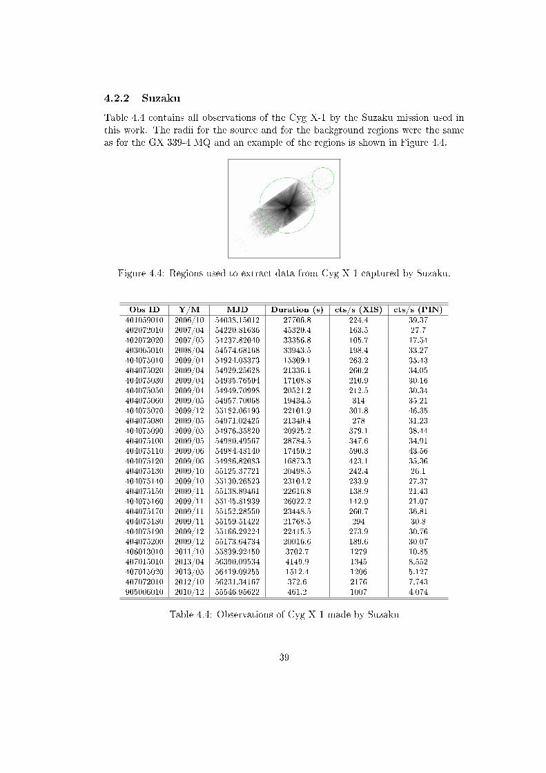
Table 4.4 contains all observations of the Cyg X-1 by the Suzaku mission used inthis work. The radii for the source and for the background regions were the sameas for the GX 339-4 MQ and an example of the regions is shown in Figure 4.4.

Figure 4.4: Regions used to extract data from Cyg X-1 captured by Suzaku.

Obs ID Y/M MJD Duration (s) cts/s (XIS) cts/s (PIN)

401059010 2006/10 54038.15012 27706.8 224.4 39.37402072010 2007/04 54220.81636 45320.4 163.5 27.7402072020 2007/05 54237.82040 33356.8 105.7 17.54403065010 2008/04 54574.68168 33943.5 198.4 33.27404075010 2009/04 54924.05373 15309.1 263.2 35.43404075020 2009/04 54929.25628 21336.1 260.2 34.05404075030 2009/04 54935.76504 17108.8 210.9 30.16404075050 2009/04 54949.70998 20521.2 212.5 30.34404075060 2009/05 54957.70068 19434.5 314 35.21404075070 2009/12 55182.06193 22101.9 301.8 46.35404075080 2009/05 54971.02425 21340.4 278 31.23404075090 2009/05 54976.35820 20925.2 379.1 38.44404075100 2009/05 54980.49567 28784.5 347.6 34.91404075110 2009/06 54984.48140 17450.2 590.3 43.56404075120 2009/06 54986.82083 16873.3 423.1 35.36404075130 2009/10 55125.37721 20498.5 242.4 26.1404075140 2009/10 55130.26523 23104.2 233.9 27.37404075150 2009/11 55138.89461 22616.8 138.9 21.43404075160 2009/11 55145.81939 26022.2 142.9 21.07404075170 2009/11 55152.28550 23448.5 260.7 36.81404075180 2009/11 55159.51422 21768.5 294 30.8404075190 2009/12 55166.29224 22415.5 273.9 30.76404075200 2009/12 55173.64734 20016.6 189.6 30.07406013010 2011/10 55839.92450 3702.7 1279 10.85407015010 2013/04 56390.09534 4149.9 1345 8.552407015020 2013/05 56419.09255 1512.4 1206 5.127407072010 2012/10 56231.34167 372.6 2176 7.743905006010 2010/12 55546.95622 461.2 1007 4.074

Table 4.4: Observations of Cyg X-1 made by Suzaku

39

Chapter 5

GX 339-4

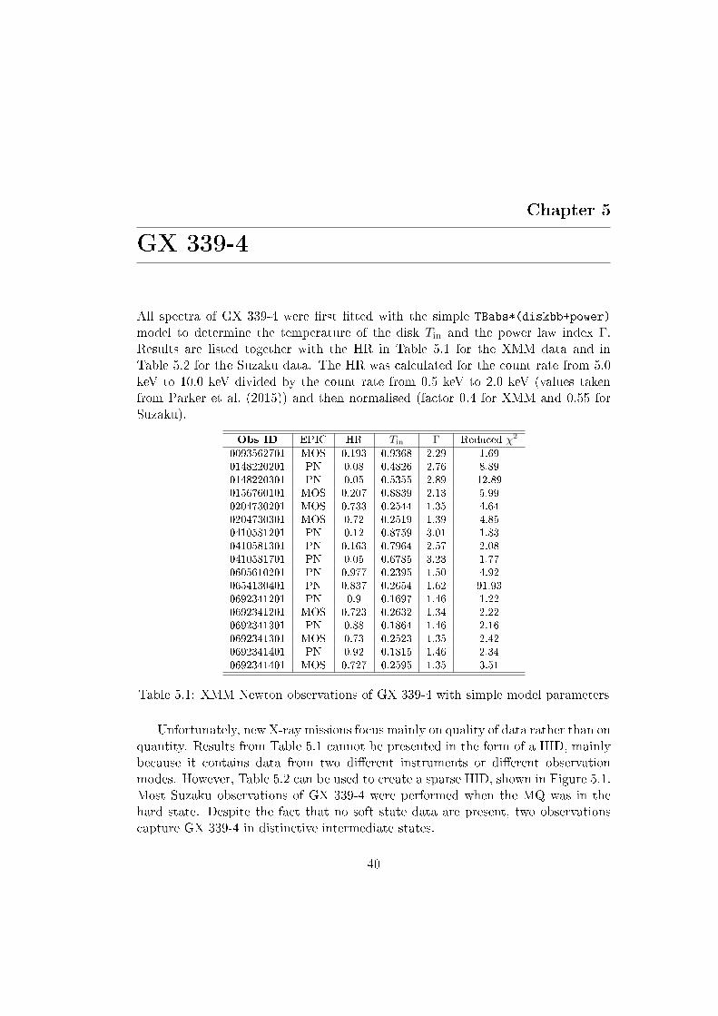
All spectra of GX 339-4 were �rst �tted with the simple TBabs*(diskbb+power)

model to determine the temperature of the disk Tin and the power law index Γ.Results are listed together with the HR in Table 5.1 for the XMM data and inTable 5.2 for the Suzaku data. The HR was calculated for the count rate from 5.0keV to 10.0 keV divided by the count rate from 0.5 keV to 2.0 keV (values takenfrom Parker et al. (2015)) and then normalised (factor 0.4 for XMM and 0.55 forSuzaku).

Obs ID EPIC HR Tin Γ Reduced χ2

0093562701 MOS 0.193 0.9368 2.29 1.690148220201 PN 0.08 0.4826 2.76 8.890148220301 PN 0.05 0.5355 2.89 12.890156760101 MOS 0.207 0.8839 2.13 5.990204730201 MOS 0.733 0.2544 1.35 4.640204730301 MOS 0.72 0.2519 1.39 4.850410581201 PN 0.12 0.8759 3.01 1.830410581301 PN 0.163 0.7964 2.57 2.080410581701 PN 0.05 0.6785 3.23 1.770605610201 PN 0.977 0.2395 1.50 4.920654130401 PN 0.837 0.2654 1.62 91.930692341201 PN 0.9 0.1697 1.46 1.220692341201 MOS 0.723 0.2632 1.34 2.220692341301 PN 0.88 0.1864 1.46 2.160692341301 MOS 0.73 0.2523 1.35 2.420692341401 PN 0.92 0.1815 1.46 2.340692341401 MOS 0.727 0.2595 1.35 3.51

Table 5.1: XMM Newton observations of GX 339-4 with simple model parameters

Unfortunately, new X-ray missions focus mainly on quality of data rather than onquantity. Results from Table 5.1 cannot be presented in the form of a HID, mainlybecause it contains data from two di�erent instruments or di�erent observationmodes. However, Table 5.2 can be used to create a sparse HID, shown in Figure 5.1.Most Suzaku observations of GX 339-4 were performed when the MQ was in thehard state. Despite the fact that no soft state data are present, two observationscapture GX 339-4 in distinctive intermediate states.

40

Obs ID HR Tin Γ Reduced χ2

401068010 0.27 0.755 2.01 11.44403011010 0.88 0.401 1.39 2.22403011020 0.87 0.412 1.39 2.24403011030 0.87 0.431 1.37 2.22403067010 0.93 0.598 1.51 1.25405063010 0.43 0.315 1.75 1.84405063020 0.69 0.283 1.60 1.43405063030 0.88 0.483 1.53 1.12405063040 0.91 0.601 1.53 1.06405063050 0.91 0.629 1.55 0.99408034010 0.88 0.326 1.45 6.98

Table 5.2: Suzaku observations of GX 339-4 with simple model parameters

In comparison with the HID in Figure 1.2, the observation 401068010 fromTable 5.2 is located near the observations of GX 339-4 in SPL state. However,the parameters do not meet the conditions of the SPL state, but it still appearsto contain the re�ection component. Figure 5.2 shows that a simple power lawmodel cannot describe this spectrum. The o�set around the 20 keV is caused bythe Compton hump typical for the re�ected radiation.

1

10

100

1000

0.1 1

Inte

nsity (

cts

/s)

HR

Figure 5.1: HID of Suzaku observations of GX 339-4

In Figure 5.2, there are many line-like features around 2 keV. These featureshave origin in the instrument. There are both absorption features, e.g. K-shell lineof aluminium (1.56 keV), and emission features, mainly M-shell lines from gold inthe XRT instrument around 2 keV. ([ex]) These features can be �tted with simpleGaussian lines, but it is a common practice to leave them out from the �ttingprocess.

41

0.1

1

ke

V (

Ph

oto

ns c

m−

2 s

−1 k

eV

−1)

102 5 20

1

0.5

2

ratio

Energy (keV)

Figure 5.2: Spectrum of GX 339-4 folded with a simple model (407072010) andmodel to data ratio

5.1 Fitting re�ection

The re�ection component in Figure 5.2 allowed for use of the RELXILL model. Thismodel was used together with an absorption model and a multi blackbody modelfor the observation 401068010. The results of �tting TBabs*(diskbb+relxill) areshown in Table 5.3. The column �input� contains parameter values or boundariesset before the �tting. Where empty, default values were used. Parameters Rin,Rout and z were frozen at their default value and angleon was set to 1. As for theinstrument related features, regions 1.5�1.95 keV, 2.1�2.4 keV and 3.0�3.3 keV wereomitted from the �tting process.

Model Parameter Input Result Error

TBabs nH 0.5-0.65 0.587 0.006DISKBB Tin 0.1-1.5 0.828 0.006DISKBB norm � 805.529 23.282RELXILL Index1 � 9.999 2.210RELXILL Index2 � 5.307 0.178RELXILL Rbr � 1.861 0.066RELXILL a � 0.997 0.004RELXILL Incl 20.0�60.0 50.199 1.189RELXILL gamma � 2.137 0.011RELXILL logxi � 2.783 0.025RELXILL Afe � 0.981 0.057RELXILL re�_frac � 10.007 3.010RELXILL norm � 0.012 0.003

χ2red = 1.376 for 1055 DOF

Table 5.3: Model parameters for 401068010

42

The result is presented in Figure 5.3. The omitted parts of the spectrum (e.g.above 8.5 keV for the XIS data) were left out due to high uncertainties. The inclina-tion of the disc is the most important result of this �t. It allows for the estimationof the BH mass from its mass function. Even though XSPEC by default works withthe con�dence level of 90%, an error of 2 degrees will be used for the inclination inorder to include any other possible statistical errors. Using f(M) = 5.8±0.5 andq = 0.08, the resulting BH mass is ≈ 15±2.5 M�.

0.1

1

keV

(P

hoto

ns c

m−

2 s

−1 k

eV

−1)

102 5 20

0.9

1

1.1

ratio

Energy (keV)

Figure 5.3: RELXILL model applied to 401068010 and model to data ratio

Figure 5.4 contains a contour from the steppar command of XSPEC for theinclination. It shows the local minimum for the �tting around the resulting inclina-tion. This value was further used as an input parameter for the BHSPEC model inorder to obtain a second BH mass estimate directly from this model.

47 48 49 50 51 52

1500

1550

1600

1650

Sta

tistic:

χ2

Parameter: Incl (deg)

Figure 5.4: Contour of the steppar command for applied to Figure 5.3

43

5.2 BHSPEC �tting

The model combination TBabs*(bhspec+power) was �rst used for the same obser-vation, but only for the XIS instrument data. The inclination, nH parameter andpower law photon index were frozen at the values obtained from the RELXILLmodel. The other parameters were left free to vary.

This procedure was then repeated for multiple observations of the XMM Newtonwith only the inclination being frozen. In order to choose the observations suitablefor this procedure, the conditions were set for the HR to be below 0.2 and the Tin tobe above 0.6 keV. These conditions were met within these observations: 0093562701,0410581201, 0410581301, 0410581701.

Table 5.4 contains parameters obtained from �tting the Suzaku observation401068010 with the BHSPEC model. Again, there are parts of the spectrum around2 keV energy that were left out. The spectrum is presented in Figure 5.5 (a) to-gether with the steppar test (b) of the inclination. The log mass parameter is1.048±0.171 what gives BH mass ≈ 11.2±4.4 M�.


TBabs nH 0.587 0.587 �BHSPEC log mass � 1.048 0.171BHSPEC log lumin � -1.075 0.062BHSPEC inc 0.640 0.640 �BHSPEC spin � 0.792 0.057BHSPEC norm � 0.596 0.294

POWERLAW PhoIndex 2.137 2.137 �POWERLAW norm � 2.254 0.005

χ2red = 2.172 for 1024 DOF


1

0.2

0.5

2

keV

(P

hoto

ns c

m−

2 s

−1 k

eV

−1)

2 5

0.9

0.95

1

1.05

ratio

Energy (keV)

(a) Spectrum folded with model (top) andmodel to data ratio (bottom)

1 1.02 1.04 1.06 1.08 1.1

2225

2230

2235

2240

2245

Sta

tistic:

χ2

Parameter: log mass

(b) steppar contour

Figure 5.5: BHSPEC model applied to 401068010

44

Observation carried out by the XMM Newton used in this procedure requiredvery individual approach. The data are from both PN and MOS instruments andboth imaging and burst modes. The observations 0410581201 and 0410581701 were�tted using the same models combination as in the previous step. The results arelisted in Table 5.5. The BH mass estimates are 14.1±5.4 M� and 15.7±8.2 M�for 0410581201 and 0410581701, respectively.

Observation ID 0410581201 0410581701

Model Parameter Input Result Error Input Result Error

TBabs nH 0.5-0.7 0.629 0.012 0.5-0.7 0.680 0.026BHSPEC log mass � 1.15 0.165 � 1.197 0.227BHSPEC log lumin � �1.249 0.106 � �1.605 0.224BHSPEC inc 0.640 0.640 � 0.640 0.640 �BHSPEC spin � 0.99 0.03 � 0.98 0.02BHSPEC norm � 3.406 1.969 � 2.921 2.189

POWERLAW PhoIndex � 3.031 0.059 � 3.424 0.059POWERLAW norm � 3.389 0.442 � 2.976 0.273

χ2red = 1.313 for 157 DOF χ2

red = 1.213 for 144 DOF

Table 5.5: Model parameters for 0410581201 and 041581701

The spectra are shown in Figure 5.6 for observation number 041058120 and inFigure 5.7 for observation number 0410581701. These two observations were carriedout by the PN instrument in burst mode and were possible to be �tted with theTBabs*(bhspec+power) model.

0.1

1

keV

(P

hoto

ns c

m−

2 s

−1 k

eV

−1)

1 2 5

0.8

1

1.2

ratio

Energy (keV)


1.05 1.1 1.15 1.2 1.25 1.3

210

215

220

225

Sta

tistic:

χ2

Parameter: log mass

(b) steppar contour


Again, the spectra with ratio data×model and the contour of steppar commandare present. In Figure 5.6 (b), the model seems to have two local minima close toeach other. However, the error of the log mass parameter from Table 5.5 coversboth values.

45

10−4

10−3

0.01

0.1

1

keV

(P

hoto

ns c

m−

2 s

−1 k

eV

−1)

1 2 50

0.5

1

1.5

ratio

Energy (keV)


1.05 1.1 1.15 1.2 1.25 1.3 1.35 1.4

185

190

195

Sta

tistic:

χ2

Parameter: log mass

(b) steppar contour


The shape of the spectrum in Figure 5.7 (a) appears to di�er from the one inFigure 5.6 (a). The count rate of the observation number 0410581701 is lower aswell as the value of HR. This might imply that the spectrum of observation number0410581201 corresponds to the SPL state and the observation number 0410581701was performed when the GX 339-4 was in the thermal state.

The two following observations required more complicated approach. The ob-servation number 0410581301 is presented in Figure 5.8. Instead of a simple powerlaw model, broken power law model had to be used in order to properly describe thespectrum. The break energy of the model is very near the iron Kα line. Nonethe-less, including the iron line models did not �t in very well, so the broken power lawmodel was used instead. The results are presented in Table 5.6. Using the log mass

parameter value, the BH mass estimate for this observation number is 14.7±8 M�.


TBabs nH 0.5-0.7 0.642 0.007BHSPEC log mass � 1.168 0.237BHSPEC log lumin � �1.389 0.246BHSPEC inc 0.640 0.640 �BHSPEC spin � 0.983 0.021BHSPEC norm � 2.186 1.709

BKNPOWER PhoIndx1 � 2.608 0.035BKNPOWER BreakE � 6.876 0.352BKNPOWER PhoIndx2 � 3.175 0.162BKNPOWER norm � 5.174 0.358

χ2red = 1.359 for 159 DOF


It is noticeable that the count rate of this observation is higher than that seenin Figure 5.7. The observation number 0410581301 was performed when GX 339-4was in a distinctive SPL state. This might be the reason of the high uncertainty of

46

the mass estimation. The BHSPEC model is most suitable for the thermal state,when the accretion disc extends down to the ISCO. In the case of a truncation ofsome innermost regions, the model might not be able to describe the spectrum verywell. However, the contour presented in Figure 5.7 (b) shows a nice local minimumfor the acquired log mass value, yet with large uncertainty.

0.1

1

0.2

0.5

2

5

keV

(P

hoto

ns c

m−

2 s

−1 k

eV

−1)

1 2 50.8

1

1.2

1.4

ratio

Energy (keV)


1.05 1.1 1.15 1.2 1.25 1.3 1.35 1.4

217

218

219

220

Sta

tistic:

χ2

Parameter: log mass

(b) steppar contour


The last observation used in this procedure was 0093562701, where the spectrumwas extracted from the MOS instrument operating in imaging mode. As this instru-ment has a smaller energy range, there are large uncertainties appearing at energieslower than for the PN instrument. Moreover, this spectrum required, besides thebroken power law model, an addition of a Gaussian line due to an emission line-likefeature near 8 keV.


TBabs nH 0.5-0.7 0.562 0.021BHSPEC log mass � 1.293 0.214BHSPEC log lumin � �0.979 0.289BHSPEC inc 0.640 0.640 �BHSPEC spin � 0.990 0.028BHSPEC norm � 0.260 0.213

BKNPOWER PhoIndx1 � 2.115 0.112BKNPOWER BreakE � 102.99 4.352BKNPOWER PhoIndx2 � 1.987 0.254BKNPOWER norm � 0.432 0.032GAUSSIAN LineE 7.5-8.5 7.960 0.108GAUSSIAN Sigma � 0.571 0.159GAUSSIAN norm � 0.005 0.002



47

The results of the �t are presented in Table 5.7, where again the log mass

parameter value has rather large uncertainty. This might be caused by the useof the Gaussian line due to the fact that the BHSPEC model appears to be verysensitive to a combination with other models. This result yields a BH mass estimateof 19.6±9.7 M�.

0.1

1

0.2

0.5

keV

(P

hoto

ns c

m−

2 s

−1 k

eV

−1)

1 2 5

0.8

0.9

1

1.1

ratio

Energy (keV)


1.22 1.24 1.26 1.28 1.3 1.32

189

189.0

5189.1

189.1

5189.2

189.2

5

Sta

tistic:

χ2

Parameter: log mass

(b) steppar contour


As seen in Figure 5.9 (a), a short range of data had to be excluded near 2.2 keVdue to instrumental features. This exclusion served only to decrease the χ2 testvalue and did not have a large e�ect on the output parameters. The contour inFigure 5.9 (b) shows that the minimum for the mass parameter was found, yet withrather high uncertainty and a better minimum at a lower value. Therefore, thisparticular result might be questionable.

48

Chapter 6

Cyg X-1

The procedure from the previous chapter was repeated step by step. First, allspectra were �tted with a simple TBabs*(diskbb+power) model. The results arepresented in Table 6.1 and in Table 6.2 for the Suzaku mission and the XMMNewtonmission, respectively. The amount of data from the Suzaku mission allowed againa creation of a sparse HID presented in Figure 6.1. The HR in Table 6.1 was againnormalised with a factor of 0.75 in order to extend to 1.

Obs ID HR Tin Γ Reduced χ2

401059010 0.551 0.802 1.36 3.191402072010 0.885 2.170 1.364 3.005402072020 0.817 1.972 1.396 2.031403065010 0.891 1.952 1.332 3.969404075010 0.536 0.739 1.399 1.679404075020 0.519 0.825 1.412 1.633404075030 0.543 0.886 1.361 1.735404075050 0.675 1.408 1.406 1.661404075060 0.449 0.729 1.455 1.885404075070 0.431 0.642 1.345 1.698404075080 0.448 0.684 1.461 1.928404075090 0.364 0.011 1.557 9.425404075100 0.255 0.626 1.348 9.078404075110 0.269 0.518 1.579 5.065404075120 0.301 0.539 1.535 1.889404075130 0.452 0.729 1.468 1.764404075140 0.508 0.772 1.437 1.854404075150 0.963 5.197 1.403 1.467404075160 0.837 1.887 1.375 1.964404075170 0.608 0.951 1.366 2.165404075180 0.461 0.564 1.492 1.332404075190 0.495 0.731 1.462 1.394404075200 0.751 11.519 1.502 1.293406013010 0.116 0.462 2.447 4.701407015010 0.099 0.493 2.539 7.688407015020 0.064 0.517 2.601 4.089407072010 0.077 0.868 2.089 54.953905006010 0.057 0.011 3.645 34.197

Table 6.1: Suzaku observations of Cyg X-1 with simple model parameters

49

100

1000

10000

0.01 0.1 1

Inte

nsity (

cts

/s)

HR

Figure 6.1: HID of Suzaku observations of Cyg X-1 (HR for the same energybands as in Figure 5.1)

All the XMM Newton observations presented in Table 6.2 are from the PNinstrument. The HR was normalised by a factor of 0.5 to fully extend the HR from0 to 1. Two observations with the lowest HR could represent Cyg X-1 in the thermalstate. This assumption was dealt with later, after searching for the inclination.

Obs ID PN mode HR Tin Γ Reduced χ2

0202400101 ti 0.169 0.302 1.99 11.180202400601 ti 0.190 0.242 1.96 3.530202401101 bu 0.089 0.005 3.23 33.240202401201 bu 0.065 0.408 2.48 8.560500880201 bu 0.903 2.588 1.39 3.620610000401 bu 0.378 0.004 1.79 13.53

Table 6.2: XMM Newton observations of Cyg X-1 with simple model parameters

In order to follow the procedure from the previous chapter, an observation car-ried out by the Suzaku had to be chosen based on the presence of the re�ectioncomponent. Five bottom observations from Table 6.1 occupy left-top corner of theHID in Figure 6.1. However, applying the RELXILL model only worked well enoughwith the observation number 407072010. All the other observations did not containthe re�ection component in a su�cient quality.

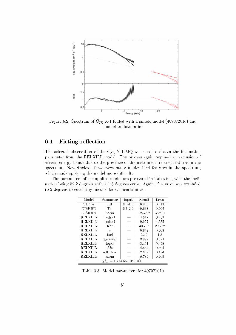
Figure 6.2 shows the spectrum of the particular observation folded with thesimple TBabs*(diskbb+power) model. It is once again noticeable, that a simplepower law function is incapable of describing the spectrum. However, the data forthe Cyg X-1 MQ contain more features and distortions in the spectra. Thereforethe energy ranges had to be adjusted separately for each observation.

50

0.1

1

10

ke

V (

Ph

oto

ns c

m−

2 s

−1 k

eV

−1)

102 5 20

0.5

1

1.5

2

ratio

Energy (keV)

Figure 6.2: Spectrum of Cyg X-1 folded with a simple model (407072010) andmodel to data ratio

6.1 Fitting re�ection

The selected observation of the Cyg X-1 MQ was used to obtain the inclinationparameter from the RELXILL model. The process again required an exclusion ofseveral energy bands due to the presence of the instrument related features in thespectrum. Nevertheless, there were many unidenti�ed features in the spectrum,which made applying the model more di�cult.

The parameters of the applied model are presented in Table 6.3, with the incli-nation being 52.2 degrees with a 1.3 degrees error. Again, this error was extendedto 2 degrees to cover any unconsidered uncertainties.


TBabs nH 0.5-1.5 0.839 0.013DISKBB Tin 0.1-2.0 0.618 0.004DISKBB norm � 12473.2 3339.1RELXILL Index1 � 4.612 0.232RELXILL Index2 � 9.992 4.335RELXILL Rbr � 40.732 22.788RELXILL a � 0.948 0.008RELXILL Incl � 52.2 1.3RELXILL gamma � 2.999 0.024RELXILL logxi � 3.491 0.058RELXILL Afe � 4.554 0.394RELXILL re�_frac � 2.607 0.424RELXILL norm � 0.784 0.209



51

0.1

1

10

ke

V (

Ph

oto

ns c

m−

2 s

−1 k

eV

−1)

102 5 20

1

1.2

1.4

ratio

Energy (keV)

Figure 6.3: RELXILL model applied to 407072010 and model to data ratio

The mass function for Cyg X-1 is 0.251±0.007, with 2.78±0.39 being the massratio. (Gies et al., 2003) Using the inclination derived from the RELXILL model,the resulting BH mass estimate is 7.3±2.6 M�. The inclination was used togetherwith the BHSPEC model applied to other observation to obtain more BH massestimates.

Despite the fact that Figure 6.4 shows a nice minimum for the inclination, theratio in Figure 6.3 reveals that the model does not follow the spectrum that well.For example, it does not �t the iron line with su�cient precision and therefore, thisresult is very questionable and should be treated with caution.

46 48 50 52 54 56 58 60

1600

1650

1700

1750

Sta

tistic:

χ2

Parameter: Incl (deg)

Figure 6.4: Contour of the steppar command for applied to Figure 6.3

52

6.2 BHSPEC �tting

The �rst step was to apply the BHSPEC model to the same observation that wasused to determine the inclination. For GX 339-4, the hydrogen column density, pho-tometric index and inclination parameters were �xed to the values of the RELXILLmodel. In this case, getting better results required for the hydrogen column densityparameter to be released. The results of the �t are shown in Table 6.4.


TBabs nH � 0.669 0.008BHSPEC log mass � 0.877 0.247BHSPEC log lumin � �1.958 0.263BHSPEC inc 0.640 0.640 �BHSPEC spin � 0.836 0.103BHSPEC norm � 32.606 24.981

POWERLAW PhoIndex 2.999 2.999 �POWERLAW norm � 28.204 0.075

χ2red = 2.651 for 1124 DOF


The spectrum and the contour are shown in Figure 6.5. The iron line around6.4 keV is very prominent. However, including it into the model with either LAORmodel or just by a simple Gaussian line improved the χ2 test, but worsened the errorsof parameters, especially for the mass parameter. The contour in Figure 6.5 (b)shows that the acquired log mass value is in a very narrow minimum.

Despite the narrow minimum, the mass parameter has high error, which leadsto the BH mass estimate of 7.5±4.3 M�. This uncertainty is very high in thesense that it could allow for the mass to drop down to the bottom limit of Cyg X-1actually being a BH.

1

10

0.5

2

5

20

keV

(P

hoto

ns c

m−

2 s

−1 k

eV

−1)

2 5

0.8

1

1.2

ratio

Energy (keV)


0.65 0.7 0.75 0.8 0.85 0.9 0.95 1 1.05

2990

3000

3010

Sta

tistic:

χ2

Parameter: log mass

(b) steppar contour


53

The observation number 407015010 by the Suzaku satellite provided a very badestimate for the BH mass. The parameters are presented in Table 6.5, where theerror of the log mass parameter is extremely high. The �t itself is very inaccuratedue to many unidenti�ed features of the spectrum. Even the overall shape of thespectrum is in disagreement with the BHSPEC model. The process required anaddition of a Gaussian line to stabilize the mass parameter. The �nal BH massestimate is 7.5 M�. The error of the BH mass is unusable in this case.



POWERLAW PhoIndex � 5.336 0.102POWERLAW norm � 66.991 2.532GAUSSIAN LineE � 6.268 0.041GAUSSIAN Sigma 1.779 0.039 �GAUSSIAN norm � 0.281 0.011

χ2red = 3.468 for 1037 DOF


The most problematic feature in Figure 6.6 (b) is the unstable minimum for thelog mass parameter. The acquired value is at a minimum that applies only to asmall range of the parameter. The contour shows that there are values with betterχ2 test results. The ratio in Figure 6.6 (a) shows that the �nal folded model doesnot follow the data very well.

1

10

0.5

2

5

keV

(P

hoto

ns c

m−

2 s

−1 k

eV

−1)

1 2 50.9

1

1.1

ratio

Energy (keV)


0.85 0.9 0.95 1

3580

3585

3590

3595

Sta

tistic:

χ2

Parameter: log mass

(b) steppar contour


54

Better results were obtained from applying the model to the observation num-ber 407015020 made by the Suzaku satellite. Table 6.6 presents the values of theparameters. Instead of the simple power law, the broken power law was requiredto get the best �t. However, the log mass parameter still has a rather high error.The BH mass estimate is 23.5±17.1 M�.



BKNPOWER PhoIndx1 � 5.283 0.087BKNPOWER BreakE � 1.984 0.012BKNPOWER PhoIndx2 2.787 0.022 �BKNPOWER norm � 50.266 2.099

χ2red = 1.769 for 1231 DOF


The high mass uncertainty is again caused by the unstable minimum noticeablein Figure 6.7 (b). The situation is similar to the contour for the observation number407015010. The minimum at which the �t is settled is very unstable. The foldedmodel in Figure 6.7 (a) appear to follow the data well, but the need to use thebroken power law might have caused the uncertainty for the mass parameter of theBHSPEC model. Besides the high error of the mass estimate, the mass itself isquite high compared to the previous results even though the values overlap by thehigh error.

1

10

0.2

0.5

2

5

keV

(P

hoto

ns c

m−

2 s

−1 k

eV

−1)

2 5

0.8

1

1.2

ratio

Energy (keV)


1.25 1.3 1.35 1.4 1.45

2174

2176

2178

2180

2182

Sta

tistic:

χ2

Parameter: log mass

(b) steppar contour


55

The observation number 406013010 made by the Suzaku satellite provides a BHmass estimate that is on the contrary very low. The results of the �t are presentedin Table 6.7 and despite the fact that the simple power law was su�cient for the �t,the χ2 test still remained higher than desired. The resulting BH mass estimate is4.7±2.1 M�. This result is very unlikely, as its lower boundary falls below the lowerBH mass limit (or rather above the top mass limit of a neutron star). (Kalogeraand Baym, 1996)



POWERLAW PhoIndex � 2.223 0.029POWERLAW norm � 5.876 0.346

χ2red = 2.855 for 1096 DOF


Figure 6.8 (a) shows that only data for energy above 1.5 keV had to be useddue to high disagreement with the model. This also prevented the exclusion of theinstrument-related artefacts to avoid corrupting the shape of the spectrum. Thismight have been the cause for the high χ2 test. Figure 6.8 (b) shows that theacquired log mass parameter is truly found in a local minimum of the contour.However, the low value of the BH mass estimate might be caused by the exclusionof the data below 1.5 keV as this part of the spectrum is created mostly by thethermal radiation.

1

10

0.5

2

5

keV

(P

hoto

ns c

m−

2 s

−1 k

eV

−1)

2 5

0.8

0.9

1

1.1

ratio

Energy (keV)


0.6 0.7 0.8 0.9 1

3130

3140

3150

3160

Sta

tistic:

χ2

Parameter: log mass

(b) steppar contour


56

The �tting of the spectrum from observation number 905006010 also required theexclusion of data below 1.5 keV. However, the log mass parameter is contrariwisequite high in comparison with the majority of the previous results. The BH massestimate is 23.7±8.1 M�. The resulting parameters are shown in Table 6.8. Thehigh χ2 is caused by the presence of the emission line-like artefacts in the spectra.They were included in the �tting for the same reason as in the previous spectrum� to prevent disruption the shape of the spectrum.




χ2red = 5.995 for 1096 DOF


In both Figure 6.8 (a) and Figure 6.9 (a) there is a slight discontinuity notice-able at approximately 4.5 keV which might be caused by an occurrence of a weakre�ection component. This is also supported by the fact that in every spectrumthe iron line is present. Therefore, it is debatable whether the observations reallycapture the Cyg X-1 MQ in the thermal state or rather in the SPL state or ina intermediate state. The contour in Figure 6.9 (b) shows that the value of thelog mass parameter was acquired at a not very stable point, as the χ2 test valuedecreases for higher log mass values.

1

0.2

0.5

2

5

keV

(P

hoto

ns c

m−

2 s

−1 k

eV

−1)

2 5

0.8

0.9

1

1.1

ratio

Energy (keV)


1.25 1.3 1.35 1.4 1.45

6540

6560

6580

6600

Sta

tistic:

χ2

Parameter: log mass

(b) steppar contour


57

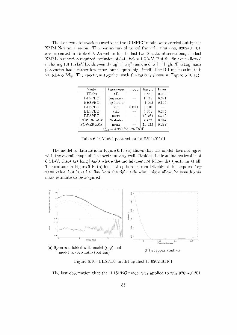
The last two observations used with the BHSPEC model were carried out by theXMM Newton mission. The parameters obtained from the �rst one, 0202401101,are presented in Table 6.9. As well as for the last two Suzaku observations, the lastXMM observation required exclusion of data below 1.5 keV. But the �rst one allowedincluding 1.0-1.5 keV bands even though the χ2 remained rather high. The log mass

parameter has a rather low error, but is quite high itself. The BH mass estimate is21.6±4.5 M�. The spectrum together with the ratio is shown in Figure 6.10 (a).






The model to data ratio in Figure 6.10 (a) shows that the model does not agreewith the overall shape of the spectrum very well. Besides the iron line noticeable at6.4 keV, there are long bands where the model does not follow the spectrum at all.The contour in Figure 6.10 (b) has a steep border from left side of the acquired log

mass value, but is rather �at from the right side what might allow for even highermass estimate to be acquired.

1

10

0.5

2

5

keV

(P

hoto

ns c

m−

2 s

−1 k

eV

−1)

1 2 5

0.9

1

1.1

ratio

Energy (keV)


1.3 1.35 1.4 1.45

650

700

750

800

850

900

Sta

tistic:

χ2

Parameter: log mass

(b) steppar contour


The last observation that the BHSPEC model was applied to was 0202401201.

58

The results are listed in Table 6.10. Features not contained in the model were notvery prominent in this observation, so the χ2 test is lower than for the previousXMM observation. However, data below 1.5 keV had to be excluded to stabilize the�t. As well as for the observation number 0202401101, the log mass parameter israther high. The BH mass estimate is 21.1±9.8 M�.






Figure 6.11 (a) shows the spectrum folded with the model and the model dataratio. In the ratio, a prominent iron line is observable. However, including this lineinto the model caused instability and drove the log mass value above 1.4 what isunreasonably high. Besides the iron line, the model seems to follow the spectrumbelow 6 keV quite well. The contour in Figure 6.11 (b) looks very similar to the oneof 0202401101. Adding iron line to the model caused the right side of the contourto drop and dragged the minimum to the right of the current one.

1

10

0.5

2

5

keV

(P

hoto

ns c

m−

2 s

−1 k

eV

−1)

2 5

0.8

0.9

1

1.1

ratio

Energy (keV)


1.3 1.35 1.4 1.45

320

340

360

Sta

tistic:

χ2

Parameter: log mass

(b) steppar contour


59

Chapter 7

Results

The aim of this work was to present a brief introduction about MQs, to providefuture readers with guides on retrieving and processing X-ray data and to makenew estimates of parameters of selected MQs. The objects that were selected forthis work were GX 339-4 and Cygnus X-1. The idea was to create a procedure thatwould be applied to the GX 339-4 MQ and then test it on the Cygnus X-1 MQ.

The results obtained for the GX 339-4 MQ are presented in Table 7.1. Thereis an estimate of the BH mass and distance to the MQ for each observation. Theinclination of the system was extracted from the RELXILL model applied to theobservation number 401068010. The estimated inclination is 50.2±2 degrees. Thisinclination was used together with the mass function of GX 339-4 to determine themass of the BH. The inclination was also used as an input for the BHSPEC model,from which the log mass parameter was extracted as another BH mass estimate.

Observation Mission MBH (M�) ∆MBH (M�) d (kpc) ∆d (kpc)

401068010a Suzaku 15.0 2.5 6.0 0.3401068010 Suzaku 11.2 4.4 13.0 3.20093562701 XMM 19.6 9.7 5.4 1.60410581201 XMM 14.1 5.4 5.9 2.20410581301 XMM 14.7 8.0 6.8 2.70410581701 XMM 15.7 8.2 19.6 8.0

Table 7.1: Results obtained for the GX 339-4 MQ. The �a� denotes the resultsderived from the RELXILL model, rest is from the BHSPEC model.

The distance to the object was calculated from the normalisation parameters ofthe models. The RELXILL model does not provide information about the distance,so the distance was computed from the norm parameter of the DISKBB modelfrom Table 5.3. It is de�ned as norm = ((Rin/km)/(d/10 kpc))2 cos i. The Rin

parameter was to ISCO and the mass derived from the mass function was used.The rest of the distance estimates in Table 7.1 was derived from the BHSPECmodel's normalisation parameter de�ned norm = (10 kpc/d)2.

60

The next step was to repeat the procedure with another object to verify theresults obtained with the GX 339-4 MQ. The parameters acquired for the Cygnus X-1 are presented in Table 7.2 for each used observation. The inclination was derivedfrom the observation number 407072010 using the RELXILL model. The inclinationestimate is 52.2±2 degrees. This value was again used together with the massfunction in order to obtain the BH mass estimate, which is presented in Table 7.2as the �rst entry. The inclination was used as an input for the BHSPEC model,from which the other BH mass estimates in the table were derived.

Observation Mission MBH (M�) ∆MBH (M�) d (kpc) ∆d (kpc)

407072010a Suzaku 7.3 2.6 0.1 0.02407072010 Suzaku 7.5 4.3 1.8 0.7407015010 Suzaku 7.8 � 5.4 �407015020 Suzaku 23.5 17.1 5.9 2.6406013010 Suzaku 4.8 2.2 1.5 0.3905006010 Suzaku 23.7 8.1 6.1 1.10202401101 XMM 21.6 4.5 2.3 0.40202401201 XMM 21.1 9.8 2.4 0.9

Table 7.2: Results obtained for the Cygnus X-1 MQ. The �a� denotes the resultsderived from the RELXILL model, rest is from the BHSPEC model.

The distance to the MQ was computed in the same way as for the GX 339-4MQ. The inclination for the �rst entry in Table 7.2 was derived from the DISKBBmodel and the rest was derived from the BHSPEC model. The observation number407015010 lacks the error values for both BH mass and distance estimates. Thesevalues were omitted because of their size, which exceeded the estimates.

61

Chapter 8

Discussion

The biggest problem when applying models to data is that the models usually corre-spond only to certain spectral components that need to be contained in the spectraand respond to the state of an object. If an object does not exhibit a re�ectioncomponent, applying the RELXILL model will not provide reasonable information.The identi�cation of the state of an object is crucial in deriving estimates of itsparameters.

The results presented in Table 7.1 may appear somewhat incorrect compared tothe most recent estimates listed in Chapter 2. Despite some diversity, the BH massestimates in Table 7.1 mostly overlap thanks to their errors, but are a bit larger thanthe recently published values. However, the estimates derived from the BHSPECmodel are in agreement with the BH mass estimate derived from the mass functionusing the system inclination. The inclination falls within the 20�60 degrees limitand is quite close to the recently published inclination of 48±1 degrees (Garcíaet al., 2015). Therefore the inclination and the BH mass estimate of 15±4 M� canbe considered suitable.

As for the distance to the GX 339-4 MQ, Table 7.1 contains a distance derivedfrom the norm parameter of the DISKBB model and distances derived from thenorm parameter of the BHSPEC model. Except two cases, the values span around∼6�7 kpc with the error of ∼2 kpc. This is in good agreement with recentlypublished values, e.g. 8.4 kpc (Parker et al., 2015) or ≥7 kpc (Zdziarski et al.,2004).

The spin of the BH of the GX 339-4 is generally considered to be nearly maximal,which corresponds to the results acquired from both the RELXILL model and theBHSPEC model. Except for the value presented in Table 5.4. The spin estimationrequires the MQ to be in the thermal or the SPL state as the spin is determinedfrom the Rin of the disc. In the cases when the disc is not extended down to theISCO, the spin estimate cannot be acquired correctly. The spin of the BH containedwithin GX 339-4 was estimated to be ≥0.98.

The Cygnus X-1 MQ was supposed to be used as a veri�cation for the procedureused. However, the results derived for the Cygnus X-1 MQ appear to di�er fromthe recently published values. This does not necessarily mean that the procedure isincorrect. It is important to assess everything that might have a�ected the process.

62

The most important aspect that needs to be considered is the fact that theCygnus X-1 MQ is a HMXB. The GX 339-4 is on the contrary a LMXB. Thatmeans that the procedure applied to the latter does not necessarily need to workwith the former the same way. When studying a HMXB, the absorption arisesnot only from the interstellar matter, but can contain a distinctive portion relatedto the MQ itself. The hydrogen column density of the Cygnus X-1 MQ is highlyvariable and can be related to the orbital movement of the components of the system.(Grinberg et al., 2015) The stream of the material from the donor star can be muchmore widespread than in the case of a LMXB and create regions of concentratedmass crossing the LOS. As the variability a�ects mostly the energies related to thedisc component of the spectrum, an uncertain determination of the absorption maycorrupt the �tting of the thermal component.

The inclination found in the recent articles is ∼30 degrees. (Zióªkowski, 2014)However, the inclination derived from the RELXILL model is 52.2±2 degrees,which is much more than generally accepted values. The combination of the 30 de-grees inclination and the mass function of the Cygnus X-1 MQ provides an unrea-sonably high mass of 29 M�. The BH mass estimate derived from the 52.2 degreesinclination is 7.3±2.6 M�. Unfortunately the other BH mass estimates presentedin Table 7.2 vary a lot. The estimates range from 4 M� up to 24 M�. The uncer-tainty of determining the mass of the BH can be assigned to improper determinationof the nH parameter of the absorption component.

The spin of the BH within the Cygnus X-1 MQ is thought to be high, but a widerange of spins was acquired when applying the BHSPEC model. This problem mayagain arise from the variable absorption component. Moreover, the observationsused with the model do not necessarily need to be captured when the MQ was inthe thermal state but rather in a similar intermediate state.

The distance of this object is well-established with parallax measurement andtherefore is very reliable. It was measured to be 1.86+0.12

−0.11 kpc (Reid et al., 2011).However, only a few estimates of the distance in Table 7.2 are close to this value.Most values are very di�erent.

The parameters acquired for the Cygnus X-1 MQ vary a lot from the recentlypublished values. However, this fact does not make the procedure applied to theGX 339-4 MQ incorrect. It only proves that all the MQs cannot be addressed inthe same way as they di�er in many aspects. To verify the procedure, more MQsshould be tested. Moreover, repeating the same steps for the same type of a MQwould be appropriate.

Future work on this approach should include more objects to be studied. Mainlyobjects that resemble each other or fall into the same category. As for the GX 339-4MQ, objects like GS 1354-64 or XTE J1655-40 could be more suitable than theCygnus X-1 MQ. Furthermore, in addition to spectral analysis, timing analysiscould provide more insight into the state of a MQ and improve the application ofan appropriate model to determine the system parameters.

63

References

K. A. Arnaud. XSPEC: The First Ten Years. In G. H. Jacoby and J. Barnes, editors,Astronomical Data Analysis Software and Systems V, volume 101 of AstronomicalSociety of the Paci�c Conference Series, page 17, 1996.

G. Bao, P. Hadrava, and E. Ostgaard. Multiple images and light curves of an emit-ting source on a relativistic eccentric orbit around a black hole. The AstrophysicalJournal, 425:63�71, April 1994. doi: 10.1086/173963.

T. Chen. The determination of the GX 339-4's mass based on its 2010 outburst.In G. E. Romero, R. A. Sunyaev, and T. Belloni, editors, Jets at All Scales,volume 275 of IAU Symposium, pages 327�328, February 2011. doi: 10.1017/S1743921310016339.

S. W. Davis, O. M. Blaes, I. Hubeny, and N. J. Turner. Relativistic AccretionDisk Models of High-State Black Hole X-Ray Binary Spectra. The AstrophysicalJournal, 621:372�387, March 2005. doi: 10.1086/427278.

R. Fender. Relativistic Out�ows from X-ray Binaries ('Microquasars'). In A. W.Guthmann, M. Georganopoulos, A. Marcowith, and K. Manolakou, editors, Rel-ativistic Flows in Astrophysics, volume 589 of Lecture Notes in Physics, BerlinSpringer Verlag, page 101, 2002.

J. Frank, A. King, and D. J. Raine. Accretion Power in Astrophysics: Third Edition.UK: Cambridge University Press, January 2002.

J. García, T. Dauser, C. S. Reynolds, T. R. Kallman, J. E. McClintock, J. Wilms,and W. Eikmann. X-Ray Re�ected Spectra from Accretion Disk Models. III. AComplete Grid of Ionized Re�ection Calculations. The Astrophysical Journal,768:146, May 2013. doi: 10.1088/0004-637X/768/2/146.

J. A. García, J. F. Steiner, J. E. McClintock, R. A. Remillard, V. Grinberg, andT. Dauser. X-Ray Re�ection Spectroscopy of the Black Hole GX 339�4: Exploringthe Hard State with Unprecedented Sensitivity. The Astrophysical Journal, 813:84, November 2015. doi: 10.1088/0004-637X/813/2/84.

D. R. Gies, C. T. Bolton, R. Fender, A. Herrero, T. C. Hillwig, L. Kaper, M. V.McSwain, J. Thomson, D. J. Wallace, and P. J. Wiita. Wind Accretion and State

64

Transitions in the Black Hole Binary Cyg X-1. In American Astronomical SocietyMeeting Abstracts, volume 35 of Bulletin of the American Astronomical Society,page 1332, December 2003.

V. Grinberg, M. A. Leutenegger, N. Hell, K. Pottschmidt, M. Böck, J. A. García,M. Hanke, M. A. Nowak, J. O. Sundqvist, R. H. D. Townsend, and J. Wilms.Long term variability of Cygnus X-1. VII. Orbital variability of the focussed windin Cyg X-1/HDE 226868 system. Astronomy & Astrophysics, 576:A117, April2015. doi: 10.1051/0004-6361/201425418.

R. I. Hynes, D. Steeghs, J. Casares, P. A. Charles, and K. O'Brien. DynamicalEvidence for a Black Hole in GX 339-4. The Astrophysical Journal, 583:L95�L98,February 2003. doi: 10.1086/368108.

V. Kalogera and G. Baym. The Maximum Mass of a Neutron Star. AstrophysicalJournal Letters, 470:L61, October 1996. doi: 10.1086/310296.

R. M. Ludlam, J. M. Miller, and E. M. Cackett. Reapproaching the Spin Estimateof GX 339-4. The Astrophysical Journal, 806:262, June 2015. doi: 10.1088/0004-637X/806/2/262.

T. H. Markert, C. R. Canizares, G. W. Clark, W. H. G. Lewin, H. W. Schnopper,and G. F. Sprott. Observations of the Highly Variable X-Ray Source GX 339-4.The Astrophysical Journal, 184:L67, September 1973. doi: 10.1086/181290.

J. M. Miller. Relativistic X-Ray Lines from the Inner Accretion Disks Around BlackHoles. Annual Review of Astronomy & Astrophysic, 45:441�479, September 2007.doi: 10.1146/annurev.astro.45.051806.110555.

K. Mitsuda, H. Inoue, K. Koyama, K. Makishima, M. Matsuoka, Y. Ogawara,K. Suzuki, Y. Tanaka, N. Shibazaki, and T. Hirano. Energy spectra of low-massbinary X-ray sources observed from TENMA. Publications of the AstronomicalSociety of Japan, 36:741�759, 1984.

S. Motta, T. Muñoz-Darias, P. Casella, T. Belloni, and J. Homan. Low-frequencyoscillations in black holes: a spectral-timing approach to the case of GX 339-4.MNRAS, 418:2292�2307, December 2011. doi: 10.1111/j.1365-2966.2011.19566.x.

J. A. Orosz, J. E. McClintock, J. P. Aufdenberg, R. A. Remillard, M. J. Reid,R. Narayan, and L. Gou. The Mass of the Black Hole in Cygnus X-1. AstrophysicalJournal, 742:84, December 2011. doi: 10.1088/0004-637X/742/2/84.

A. Paizis, K. Ebisawa, H. Takahashi, T. Dotani, T. Kohmura, M. Kokubun, J. Ro-driguez, Y. Ueda, R. Walter, S. Yamada, K. Yamaoka, and T. Yuasa. Broad-BandSpectrum of the Black Hole Candidate IGR J17497-2821 Studied with Suzaku.Publications of the Astronomical Society of Japan, 61:S107�S113, January 2009.doi: 10.1093/pasj/61.sp1.S107.

65

M. L. Parker, A. C. Fabian, G. Matt, K. I. I. Koljonen, E. Kara, W. Alston, D. J.Walton, A. Marinucci, L. Brenneman, and G. Risaliti. Revealing the X-ray vari-ability of AGN with principal component analysis. MNRAS, 447:72�96, February2015. doi: 10.1093/mnras/stu2424.

M. L. Parker, J. A. Tomsick, J. A. Kennea, J. M. Miller, F. A. Harrison, D. Barret,S. E. Boggs, F. E. Christensen, W. W. Craig, A. C. Fabian, F. Fuerst, V. Grinberg,C. J. Hailey, P. Romano, D. Stern, D. J. Walton, and W. W. Zhang. NuSTARand Swift observations of the very high state in GX 339-4: Weighing the blackhole with X-rays. ArXiv e-prints, March 2016.

M. J. Reid, J. E. McClintock, R. Narayan, L. Gou, R. A. Remillard, and J. A.Orosz. The Trigonometric Parallax of Cygnus X-1. The Astrophysical Journal,742:83, December 2011. doi: 10.1088/0004-637X/742/2/83.

R. A. Remillard and J. E. McClintock. X-Ray Properties of Black-Hole Binaries.Annual Review of Astronomy & Astrophysics, 44:49�92, September 2006. doi:10.1146/annurev.astro.44.051905.092532.

H. Sreehari, N. Iyer, and A. Nandi. Constraining the mass of Galactic black holeGX 339-4. In Astronomical Society of India Conference Series, volume 12 ofAstronomical Society of India Conference Series, 2015.

J. Svoboda, M. Dovciak, R. W. Goosmann, and V. Karas. Comparison of Relativis-tic Iron Line Models. ArXiv e-prints, January 2009.

J. A. Tomsick, M. A. Nowak, M. Parker, J. M. Miller, A. C. Fabian, F. A. Har-rison, M. Bachetti, D. Barret, S. E. Boggs, F. E. Christensen, W. W. Craig,K. Forster, F. Fürst, B. W. Grefenstette, C. J. Hailey, A. L. King, K. K. Madsen,L. Natalucci, K. Pottschmidt, R. R. Ross, D. Stern, D. J. Walton, J. Wilms, andW. W. Zhang. The Re�ection Component from Cygnus X-1 in the Soft StateMeasured by NuSTAR and Suzaku. Astrophysical Journal, 780:78, January 2014.doi: 10.1088/0004-637X/780/1/78.

A. A. Zdziarski, M. Gierli«ski, J. Mikoªajewska, G. Wardzi«ski, D. M. Smith, B. A.Harmon, and S. Kitamoto. GX 339-4: the distance, state transitions, hysteresisand spectral correlations. MNRAS, 351:791�807, July 2004. doi: 10.1111/j.1365-2966.2004.07830.x.

S.-N. Zhang. Black hole binaries and microquasars. Frontiers of Physics, 8:630�660,December 2013. doi: 10.1007/s11467-013-0306-z.

J. Zióªkowski. Determination of the masses of the components of the HDE226868/Cyg X-1 binary system. MNRAS, 440:L61�L65, May 2014. doi:10.1093/mnrasl/slu002.

66

Electronic references and sources

[e1] http://www.universetoday.com

[e2] http://mintaka.sdsu.edu/faculty/orosz/web/

[e3] https://heasarc.gsfc.nasa.gov/lheasoft/download.html

[e4] https://heasarc.gsfc.nasa.gov/docs/suzaku/aehp_about.html

[e5] http://heasarc.gsfc.nasa.gov/cgi-bin/W3Browse/w3browse.pl

[e6] ftp://legacy.gsfc.nasa.gov/suzaku/doc/general/suzaku_abc_guide.pdf

[e7] http://www.cosmos.esa.int/web/xmm-newton/technical-details

[e8] http://nxsa.esac.esa.int/nxsa-web/#search

[e9] http://www.cosmos.esa.int/web/xmm-newton/download-and-install-sas

67

Appendix A - Spectrum extraction

MOS in imaging mode

evselect table=mos1U002-clean.fits withspectrumset=yes \

spectrumset=MOSsource_spectrum.fits energycolumn=PI \

spectralbinsize=5 withspecranges=yes specchannelmin=0 \

specchannelmax=11999 expression='#XMMEA_EM && \

(PATTERN<=12) && ((X,Y) IN circle(25393.5,23814.5,500))'

evselect table=mos1U002-clean.fits withspectrumset=yes \

spectrumset=MOSbackground_spectrum.fits energycolumn=PI \


specchannelmax=11999 expression='#XMMEA_EM && \

(PATTERN<=12) && ((X,Y) IN annulus(30360.5,28400.5,650,1000))'

rmfgen spectrumset=MOSsource_spectrum.fits rmfset=MOS.rmf

arfgen spectrumset=MOSsource_spectrum.fits arfset=MOS.arf \

withrmfset=yes rmfset=MOS.rmf badpixlocation=MOSclean.fits \

detmaptype=psf

specgroup spectrumset=MOSsource_spectrum.fits mincounts=25 \

oversample=3 rmfset=MOS.rmf arfset=MOS.arf \

backgndset=MOSbackground_spectrum.fits \

groupedset=MOS_spectrum_grp.fits

PN in imaging mode

evselect table=EPICclean.fits withspectrumset=yes \

spectrumset=PNsource_spectrum.fits energycolumn=PI \


specchannelmax=11999 expression='(FLAG==0) && \

(PATTERN<=4) && ((X,Y) IN circle(25393.5,23814.5,500))'


spectrumset=PNbackground_spectrum.fits energycolumn=PI \



(PATTERN<=4) && ((X,Y) IN annulus(30360.5,28400.5,650,1000))'

68

rmfgen spectrumset=PNsource_spectrum.fits rmfset=PN.rmf

arfgen spectrumset=PNsource_spectrum.fits arfset=PN.arf \

withrmfset=yes rmfset=PN.rmf \

badpixlocation=PNclean.fits detmaptype=psf

specgroup spectrumset=PNsource_spectrum.fits \

mincounts=25 oversample=3 rmfset=PN.rmf arfset=PN.arf \

backgndset=PNbackground_spectrum.fits \

groupedset=PN_spectrum_grp.fits

PN in timing mode


spectrumset=PNsource_spectrum.fits energycolumn=PI \



(PATTERN<=4) && (RAWX>=29) && (RAWX<=47)'


spectrumset=PNbackground_spectrum.fits energycolumn=PI \



(PATTERN<=4) && (RAWX>=3) && (RAWX<=5)'

backscale spectrumset=PNsource_spectrum.fits \

badpixlocation=EPICclean.fits

backscale spectrumset=PNbackground_spectrum.fits \

badpixlocation=EPICclean.fits

rmfgen spectrumset=PNsource_spectrum.fits rmfset=PN.rmf

arfgen spectrumset=PNsource_spectrum.fits arfset=PN.arf \

withrmfset=yes rmfset=PN.rmf \

badpixlocation=EPICclean.fits detmaptype=psf

specgroup spectrumset=PNsource_spectrum.fits \

mincounts=25 oversample=3 rmfset=PN.rmf arfset=PN.arf \

backgndset=PNbackground_spectrum.fits \

groupedset=PN_spectrum_grp.fits

PN in burst mode

The only di�erence in the procedure for the burst mode is an additional RAWY con-dition for the evselect command for both source and background spectrum.

expression='(FLAG==0) && (PATTERN<=4) && \

(RAWX>=3) && (RAWX<=5) && (RAWY<=140)'

69

masarykoav univerzita p°írodov¥decák...

Documents