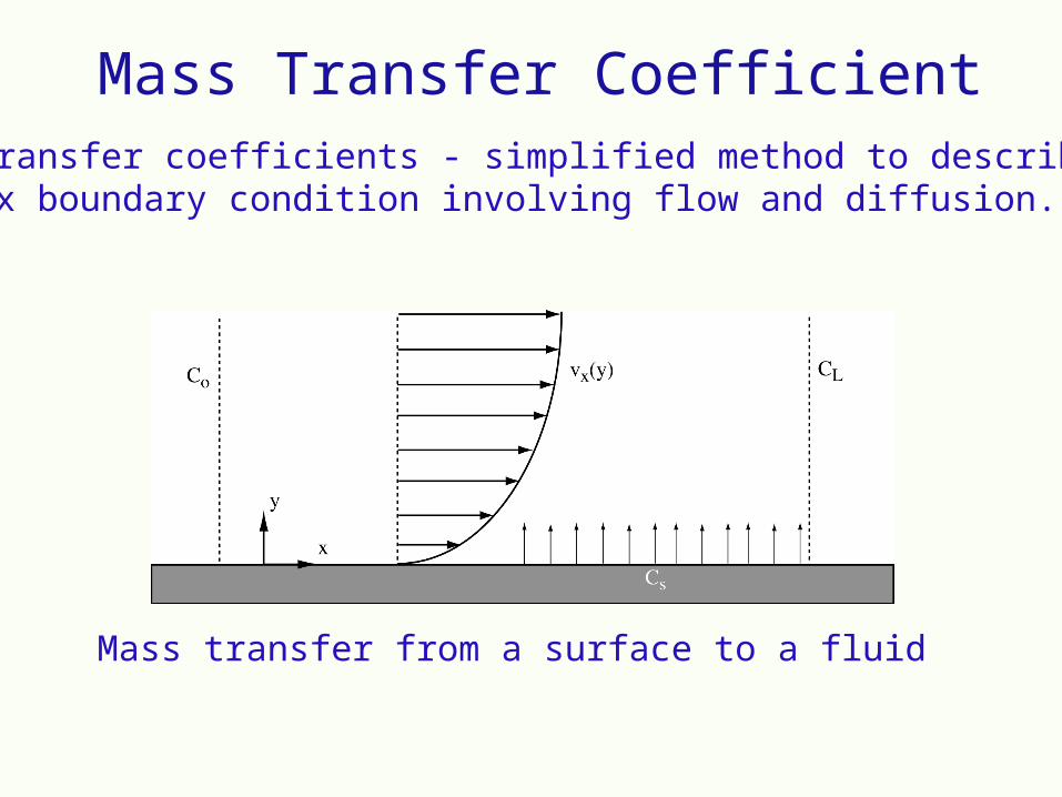
Mass transfer coefficients - simplified method to describecomplex boundary condition involving flow and diffusion.

Mass transfer from a surface to a fluid

Mass Transfer Coefficient

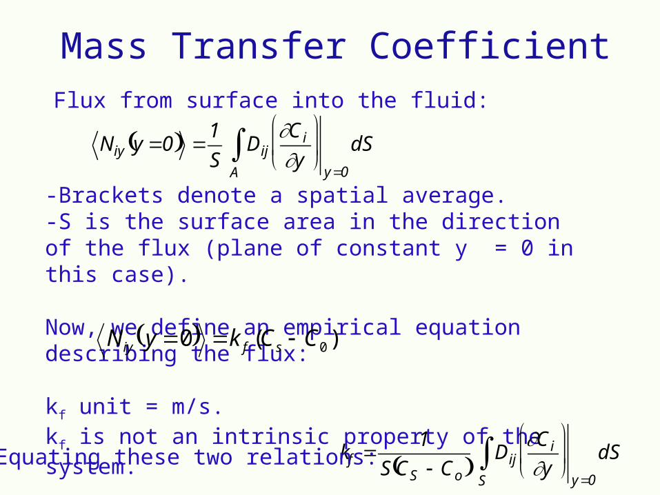
Flux from surface into the fluid:

-Brackets denote a spatial average. -S is the surface area in the direction of the flux (plane of constant y = 0 in this case).

Now, we define an empirical equation describing the flux:

kf unit = m/s. kf is not an intrinsic property of the system.

Niy y 0 1

SDij

Ciy

y0

dSA

kf 1

S CS Co Dij

Ciy

y0

dSS

Mass Transfer Coefficient

)(0 0CCkyN sfiy

Equating these two relations:

Mass Transfer Coefficient

0

*

CC

CC

s

i

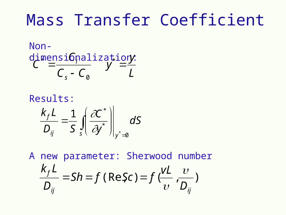
Non-dimensionalization:

L

yy *

Results:

s yij

f dSy

C

SD

Lk

0

*

*

*

1

),()(Re,ijij

f

D

vLfScfSh

D

Lk

A new parameter: Sherwood number

Mass Transfer Coefficient

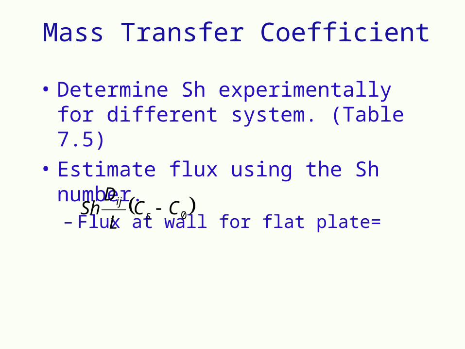
• Determine Sh experimentally for different system. (Table 7.5)

• Estimate flux using the Sh number. – Flux at wall for flat plate=

0CCL

DSh s

ij

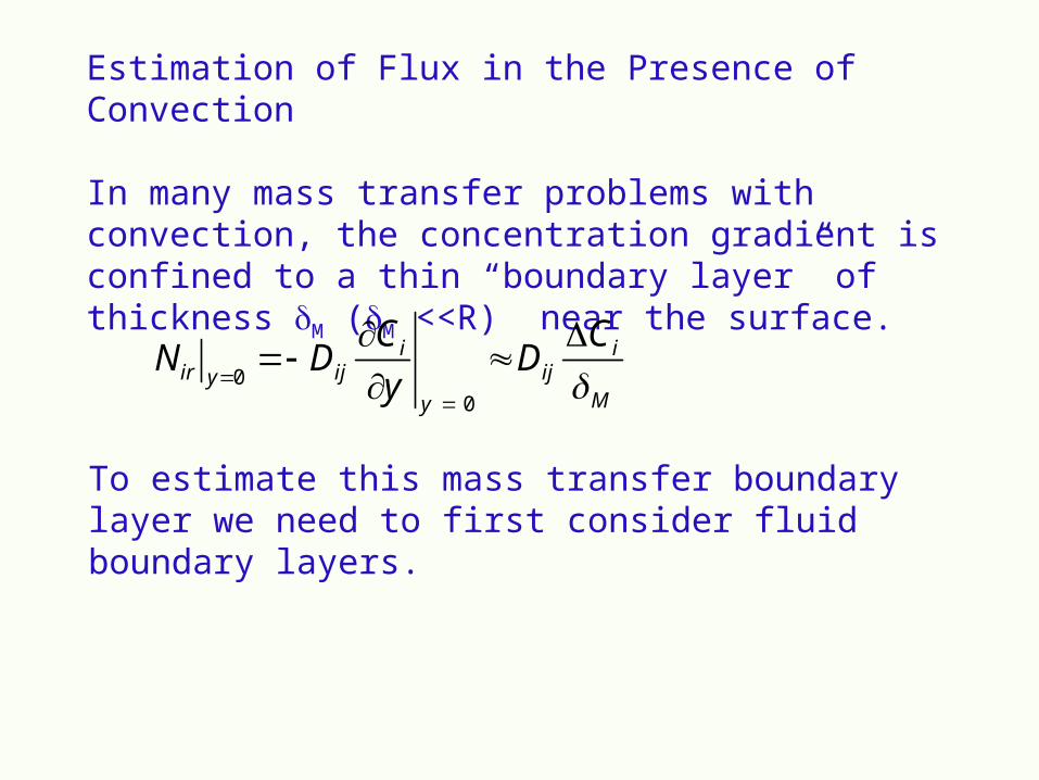
Estimation of Flux in the Presence of Convection

In many mass transfer problems with convection, the concentration gradient is confined to a thin “boundary layer” of thickness M (M <<R) near the surface.

Nir y0 Dij

Ciy

y 0

DijCiM

To estimate this mass transfer boundary layer we need to first consider fluid boundary layers.

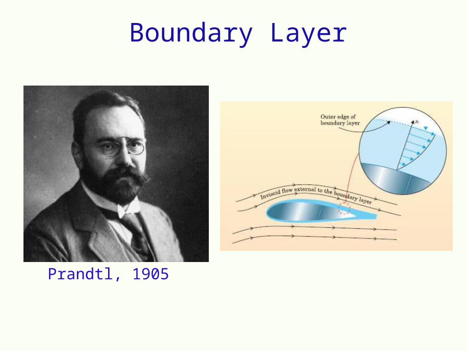
Boundary Layer

Prandtl, 1905

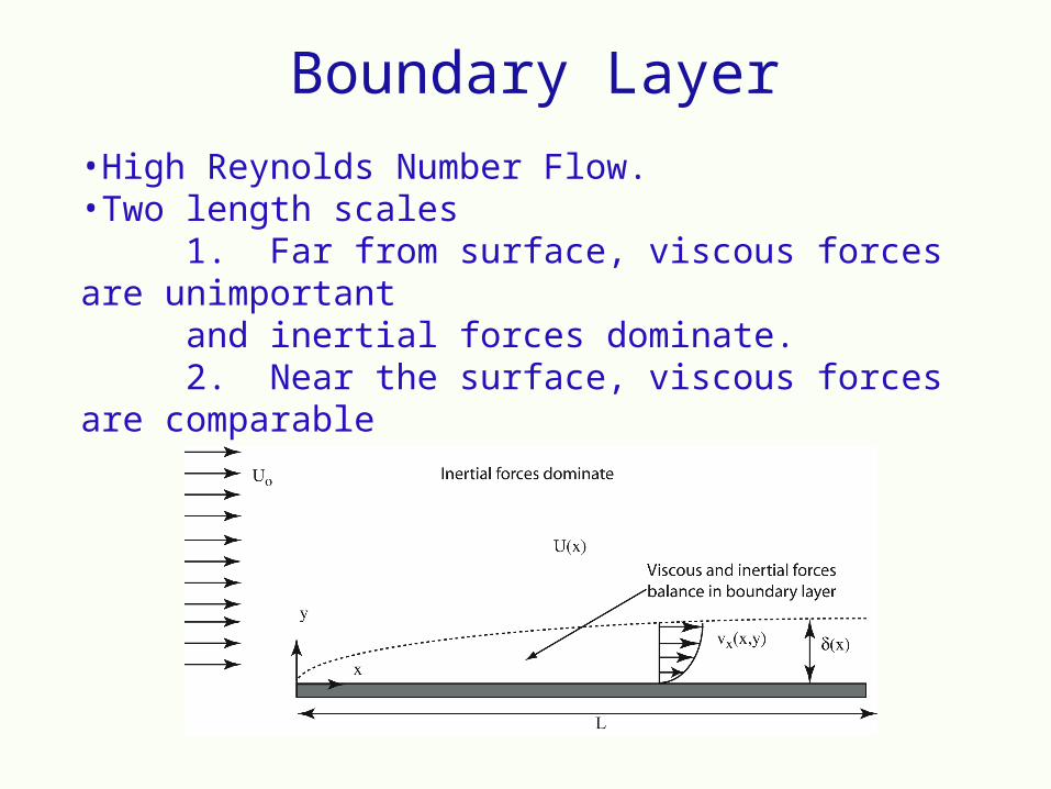
•High Reynolds Number Flow.•Two length scales

1. Far from surface, viscous forces are unimportant and inertial forces dominate.2. Near the surface, viscous forces are comparable to inertial forces

Boundary Layer

Approach:1. Perform scaling for two dimensional flow for a

boundary layer of thickness in y direction and a length scale L in the x direction.

2. Derive the “boundary layer” equations3. Examine approximate solutions to obtain boundary

layer thickness and shear stress4. Apply to mass transfer boundary layers5. Estimate mass transfer coefficients

Boundary Layer

vxx

+ vyy

= 0

vxvxx

+ vyvxy

= -P

x +

2vxx2

+ 2vxy2

vxvyx

+ vyvyy

= -P

y +

2vyx2

+ 2vyy2

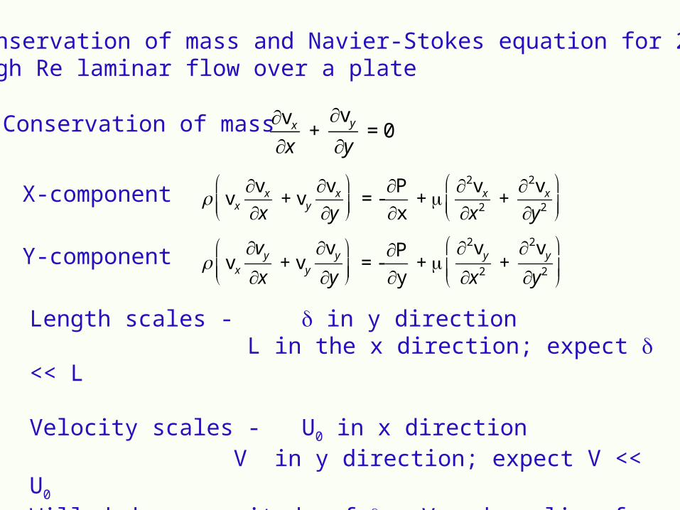
Conservation of mass and Navier-Stokes equation for 2-DHigh Re laminar flow over a plate

Length scales - in y direction L in the x direction; expect << L

Velocity scales - U0 in x directionV in y direction; expect V << U0

Will deduce magnitude of , V and scaling for pressure from an order of magnitude analysis

Conservation of mass

X-component

Y-component

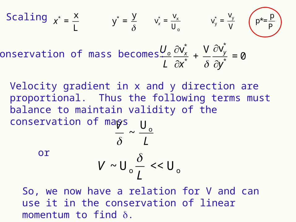
Scaling x* = x

L y* =

y

vx

* = vx

Uo

vy* =

vy

V p*=

p

P

Uo

L

vx*

x* +

V

vy

*

y* = 0Conservation of mass becomes:

Velocity gradient in x and y direction are proportional. Thus the following terms must balance to maintain validity of the conservation of mass

V ~ Uo

L

<< Uo

or

V

~

Uo

L

So, we now have a relation for V and can use it in the conservation of linear momentum to find .

Uo2

Lvx

* vx*

x* + vy

* vx*

y*

= -PL

P*

x* +

Uo

2

2

L2

2vx*

x*2 +

2vx*

y*2

x component of the conservation of linear momentum

Can neglect underlined term since 2 << LSimplifying and rearranging

Uo2

Lvx

* vx*

x* + vy

* vx*

y*

= -P 2

UoL

P*

x* +

2vx*

y*2

Since viscous and inertial forces are equally important in the boundary layer

Uo2

L~ 1

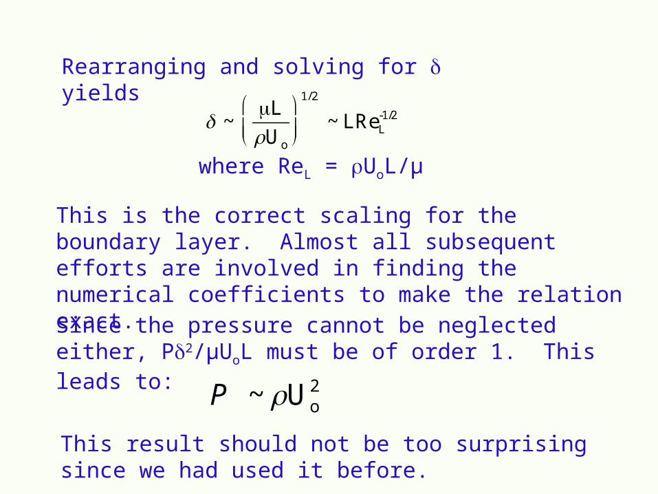
Rearranging and solving for yields

~ L

Uo

1/2

~ LReL-1/2

where ReL = UoL/µ

This is the correct scaling for the boundary layer. Almost all subsequent efforts are involved in finding the numerical coefficients to make the relation exact.

Since the pressure cannot be neglected either, P2/µUoL must be of order 1. This leads to:

P ~ Uo2

This result should not be too surprising since we had used it before.

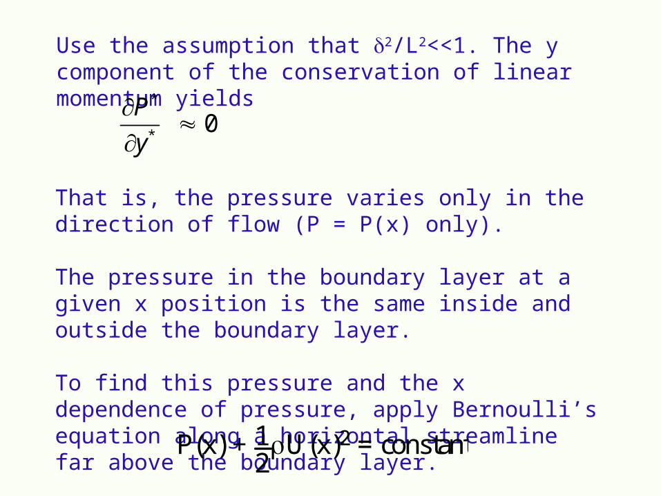
Use the assumption that 2/L2<<1. The y component of the conservation of linear momentum yields

P*

y* 0

That is, the pressure varies only in the direction of flow (P = P(x) only).

The pressure in the boundary layer at a given x position is the same inside and outside the boundary layer.

To find this pressure and the x dependence of pressure, apply Bernoulli’s equation along a horizontal streamline far above the boundary layer.

P(x) + 12U(x)2 = constant

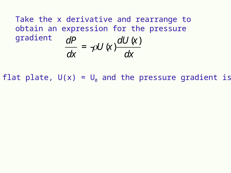
Take the x derivative and rearrange to obtain an expression for the pressure gradient

dP

dx = -U(x)

dU(x)

dx

For a flat plate, U(x) = U0 and the pressure gradient is zero.

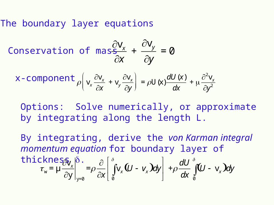
The boundary layer equations

vxx

+ vyy

= 0Conservation of mass

x-component vxvxx

+ vyvxy

= U(x)dU(x)

dx +

2vxy2

Options: Solve numerically, or approximate by integrating along the length L.

w = µvxy

y=0

=x

vx U vx dy0

+

dU

dxU vx dy

0

By integrating, derive the von Karman integral momentum equation for boundary layer of thickness .

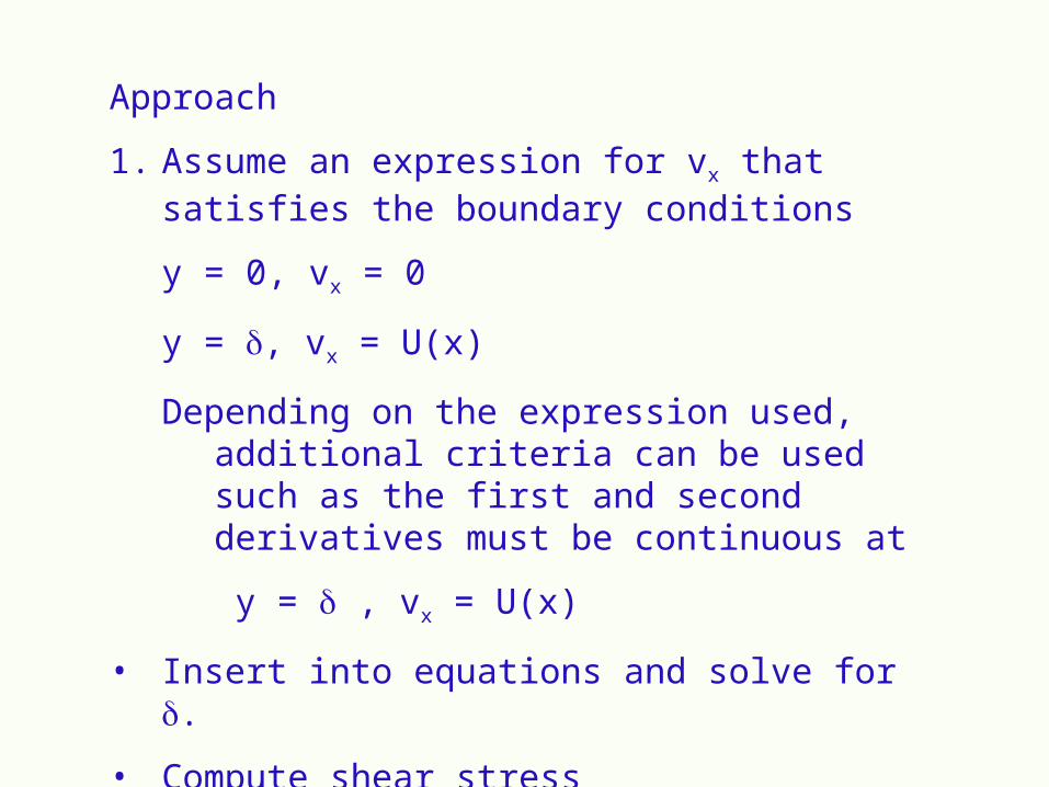
Approach

1. Assume an expression for vx that satisfies the boundary conditions

y = 0, vx = 0

y = , vx = U(x)

Depending on the expression used, additional criteria can be used such as the first and second derivatives must be continuous at

y = , vx = U(x)

• Insert into equations and solve for .

• Compute shear stress

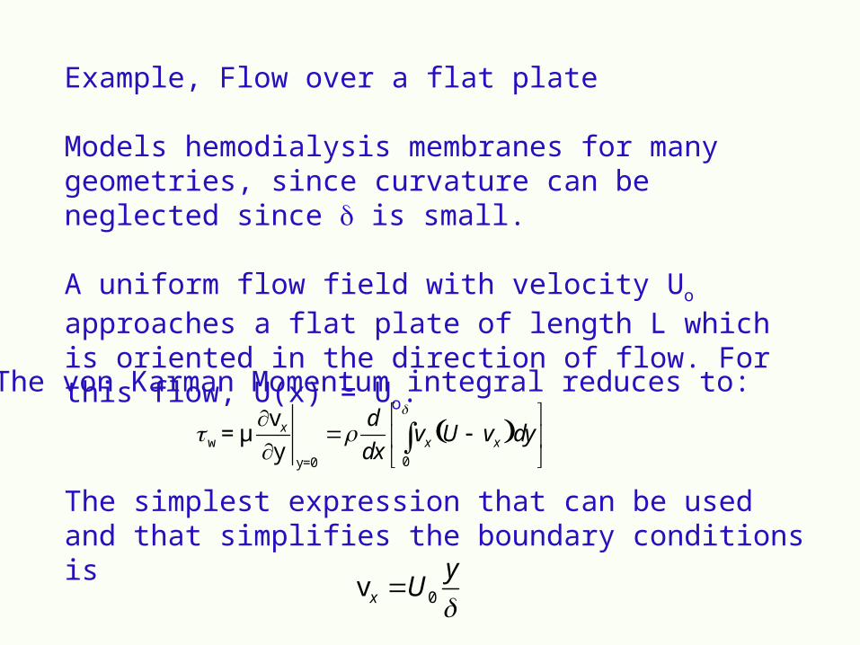
Example, Flow over a flat plate

Models hemodialysis membranes for many geometries, since curvature can be neglected since is small.

A uniform flow field with velocity Uo approaches a flat plate of length L which is oriented in the direction of flow. For this flow, U(x) = Uo.

The von Karman Momentum integral reduces to:

w = µvxy

y=0

d

dxvx U vx dy

0

The simplest expression that can be used and that simplifies the boundary conditions is

vx U0

y

Inserting this expression into the momentum integral yields

w = vx

yy=0

= Uo

=

Uo2

6

ddx

So, now we have a first order ODE for . We just need an initial which is that at x = 0, = 0.

This yields the following results

(x) = 12µxUo

= 3.464xRex-1/2

w = -0.289µUo

x Rex1/2

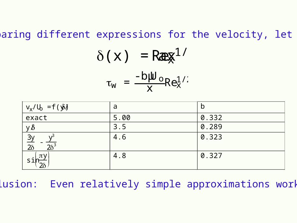
vx/Uo =f(y/ ) a b

exact 5.00 0.332 y/ 3.5 0.289

3y

2 -

y3

23 4.6 0.323

siny

2

4.8 0.327

Comparing different expressions for the velocity, let

(x) = axRex-1/2

w = -bµUo

x Rex1/2

Conclusion: Even relatively simple approximations work well

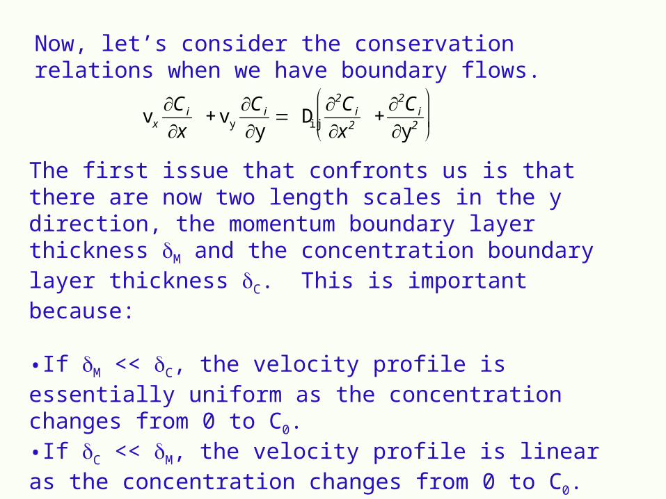
Now, let’s consider the conservation relations when we have boundary flows.

vxCix

+ vy

Ciy

Dij

2Cix 2

+2Ciy2

The first issue that confronts us is that there are now two length scales in the y direction, the momentum boundary layer thickness M and the concentration boundary layer thickness C. This is important because:

•If M << C, the velocity profile is essentially uniform as the concentration changes from 0 to C0.•If C << M, the velocity profile is linear as the concentration changes from 0 to C0.•If C ~ M,the concentration and momentum boundary layers are of the same thickness

In the non-dimensionalization of the conservation relation for solute transport, the concentration is a function of Re and Sc.

The Schmidt number controls the relative importance of momentum and diffusive transport.

For solutes in water, Sc =/Dij ranges from 103 for small solutes to 103 for proteins.

Thus, convective transport is much greater than diffusive transport and the solute concentration gradient is confined in a narrow region near the surface.

C << M Linear velocity profile, vx = Uo

y

M~ Uo

CM

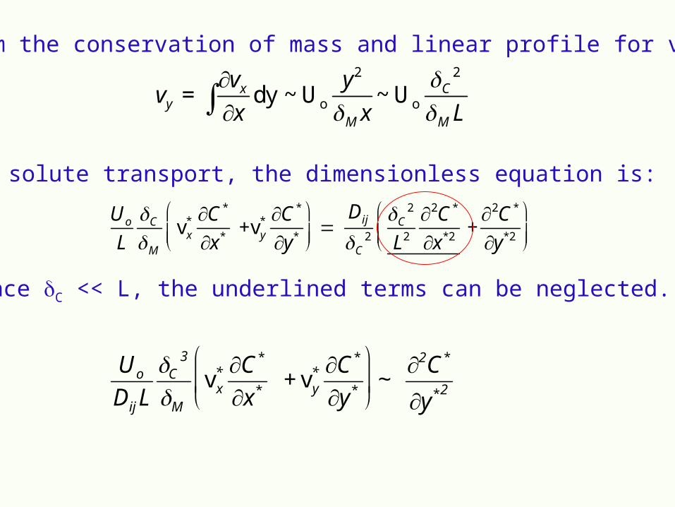
From the conservation of mass and linear profile for vx

vy = vxx

dy ~ Uo

y2

M x~ Uo

C2

ML

For solute transport, the dimensionless equation is:

Uo

L

CM

vx* C*

x* +vy

* C*

y*

DijC

2

C2

L2

2C*

x*2 +

2C*

y*2

Since C << L, the underlined terms can be neglected.

Uo

DijL

C3

Mvx* C*

x* + vy

* C*

y*

~

2C*

y*2

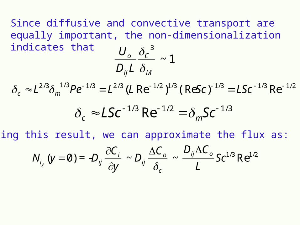
Since diffusive and convective transport are equally important, the non-dimensionalization indicates that

Uo

DijL

C3

M ~ 1

Using this result, we can approximate the flux as:

Niy(y 0) = -Dij

Ciy

~ DijCoc

~ DijCoL

Sc1/3 Re1/2

2/13/13/13/12/13/23/13/13/2 Re)(Re)Re( LScScLLPeL mc 3/12/13/1 Re ScLSc mc

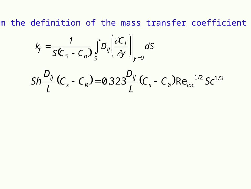
From the definition of the mass transfer coefficient

kf 1

S CS Co Dij

Ciy

y0

dSS

3/12/100 Re323.0 ScCC

L

DCC

L

DSh locs

ijs

ij