Preprint typeset in JHEP style - PAPER VERSION Part III Essay 2007

Massive Neutrinos in a Warped Extra Dimension

Philip Tanedo

Department of Applied Mathematics and Theoretical PhysicsUniversity of CambridgeCambridge, CB3 0WA, UKEmail: pt291@cam.ac.uk

Abstract: The Randall-Sundrum I (RS1) model of a warped extra dimension provides a naturalcandidate solution to the hierarchy problem between the Planck and weak scales. Coincidentally, thetheoretical development of such ‘braneworld’ models in the late 1990s coincided with the experimentalverification of nonzero neutrino masses. This presents another hierarchy problem: why are neutrinomasses vanishingly small compared to the weak scale? To solve this, Grossman and Neubert haveproposed a ‘generalized see-saw mechanism’ utilizing bulk right-handed neutrinos within the RS1framework. Such a model is highly constrained by limits on lepton flavor violation, and Kitano hasshown that some fine tuning is required to meet these bounds. In this essay I will present the RS1model, the Grossman-Neubert extension, and lepton flavor violation from RS1 bulk neutrinos.

Essay 74, The Phenomenology of Extra Dimensions. Extra dimensional models provide aninteresting playground for model building and investigating collider signatures. Candidates areinvited to provide an overview of one of the following extra-dimensional models: ADD(Arkani-Hamed, Dimopoulos and Dvali), UED (Universal Extra Dimensions) or Randall-Sundrum I.The candidate should include a calculation of a matrix element squared for a collider signature of themodel.

This essay is presented in partial fulfillment of the requirements for a Certificate of Advanced Study in

Mathematics at the University of Cambridge.

Contents

1. Introduction: The Spirit of ‘98 2

2. The RS1 Model 22.1 Welcome to braneworld 32.2 Defining the interval: Orbifolding 42.3 The wind up: The RS1 action 42.4 The pitch: RS1 background solution 52.5 A home run: Generating the hierarchy 72.6 Dust under the rug 8

3. Fermions in Extra Dimensions 93.1 Stairway to the Tangent Space 93.2 5D representations of the Clifford algebra and the chirality problem 103.3 Fermionic action in a warped extra dimension 11

4. Neutrino Masses in RS1 124.1 Leaving braneworld 124.2 Bulk fermions in RS1 124.3 Generalized see-saw from a bulk neutrino 154.4 Two bulk neutrinos are better than one 174.5 Realistic phenomenology 18

5. Lepton Flavor Violation from bulk RS1 neutrinos 195.1 Radiative charged lepton decay 205.2 Lepton flavor violation phenomenology 21

6. Summary and further directions 22

7. Acknowledgements 23

A. Notation and Convention 23

B. Properties of the RS1 bulk eigenbasis 24B.1 Orthogonality 24B.2 Differential Equation for f 24

C. Highlights of the calculation µ → eγ in RS1 with bulk neutrinos 25C.1 Lorentz structure 25C.2 Details of µ → Wνγ → eγ 26C.3 Results for the remaining diagrams 28

– 1 –

1. Introduction: The Spirit of ‘98

After three decades under the hegemony of the Standard Model/Minimally Supersymmetric StandardModel, the end of the 1990s was marked by surprising new theoretical and experimental directionsbeyond the Standard Model. In 1998-‘99, papers by Arkani-Hamed, Dimopoulos, and Dvali (ADD) [1]as well as Randall and Sundrum (RS1) [2] introduced modern1 extra-dimensional ‘braneworld’ modelsthat provided novel approaches to the hierarchy problem. The RS1 model, in particular, features awarped metric that generates a Planck-weak hierarchy with natural O(1) dimensionless parameters.

Just four months after the first of these braneworld papers, the Super-Kamiokande collaborationpublished atmospheric neutrino results indicating that neutrinos have non-zero, but very tiny, mass [5].This was the first experimental result in particle physics that required a modification of the StandardModel Lagrangian. Just when theorists had made progress on the relation between the Planck andweak scales, the discovery of these vanishingly small neutrino masses introduced a new hierarchyproblem.

The standard approach to generating this scale is through the see-saw mechanism by which mass-less left-handed neutrinos mix with a heavy right-handed neutrino to form eV-scale mass eigenstates [6].However, with the timely development of braneworld models to address the original hierarchy problem,the natural step would be to look for inherently extra dimensional solutions to the neutrino mass ques-tion. The RS1 model presents unique challenges for neutrino model-building, since there is neither anintermediate energy scale available to see-saw neutrino masses nor an appreciable extra dimensionalvolume suppression as implemented in the ADD model [7].

Grossman and Neubert have presented a minimal extension to the RS1 model where the right-handed neutrino, which is a Standard Model gauge-singlet, is allowed to propagate in the bulk [8].Suitable boundary conditions allow a zero mode that is localized on the hidden brane, utilizing the RS1warp factor to generate the neutrino mass hierarchy. This generalizes the see-saw mechanism to warpedextra dimensions. Kitano, Cheng, and Li have shown that such a model is constrained by lepton flavorviolation and that experimental bounds force some fine-tuning of model’s parameters [9, 10].

In this essay I review the RS1 model, its extension by Grossman and Neubert, and Kitano’scalculation of lepton flavor violation from µ → eγ. In Section 2 I present the RS1 model and itssolution to the hierarchy problem. In Section 3 I introduce the formalism of bulk fermions within acurved space. I then make use of this formalism in Section 4, where I discuss the Grossman-Neubertextension for neutrino masses. In Section 5 I show that such an extension generates lepton flavorviolation effects that are constrained by experimental bounds; I have included recent experimentalresults published after Kitano’s original analysis. My notation and conventions are summarized inAppendix A. Some calculations regarding the bulk fermion formalism that are not explicit in theGrossman-Neubert paper are worked out in Appendix B. The details of the calculation of the µ → eγ

amplitude in the Grossman-Neubert extension are presented in Appendix C.

2. The RS1 Model

We begin by describing the RS1 model and the mechanism by which it generates the Planck-weakhierarchy. A cartoon picture of the model is presented in Figure 1. Our observed space is actuallyone of two 3+1 dimensional branes at the endpoints of an interval in a fifth dimension. The bulk 4+1

1Here ‘modern’ is meant to distinguish these from the original braneworld scenarios developed independently in 1982

by Akama [3] and in 1983 by Rubakov and Shaposhnikov [4]. It wasn’t until ADD and RS1, however, that braneworld

models were connected to the hierarchy problem.

– 2 –

dimensional spacetime is warped in such a way that the induced metric on our brane is conformallyscaled. The measure of this rescaling is the warp factor, which is shown as a red line. We shall seethat this warping also has the effect of rescaling masses relative to the fundamental 5D Planck mass,thus generating the hierarchy. Before proceeding, some introductory remarks are in order regardingthe nature of branes.

2.1 Welcome to braneworld

Figure 1: RS1 braneworld with the

visible brane represented by Gau-

guin’s “Where Do We Come From?

What Are We? Where Are We Go-

ing?” (1897). The red line depicts

the warp factor, with the φ axis run-

ning from −π to 0.

As prompted by Gauguin’s famous painting in Figure 1, thenatural introductory questions to ask are, “Where do [branes]come from? What are [branes]? Where are [branes] going?”Following the typical response of physics students to Post-Impressionist art, the correct answer for low-energy model-builders is who cares?

We shall take Sundrum’s model-building definition of abrane as a 3+1 dimensional surface in a higher dimensionalspace where standard model particles are confined to propa-gate [11]. These objects are solitonic membranes of characteris-tic width much smaller than the scale of the low-energy effectivetheory we seek. The existence of such objects can be motivatedby a high energy theory. In string theory, for example, the end-points of open strings can be constrained to fall on so-calledD-branes. Randall-Sundrum models, in particular, are reminis-cent of Horava-Witten domain walls in M-theory [12, 13]. Butmore generally, the point is that brane-like topological defectsare allowed to exist in the low-energy effective theory of somehigh-energy theory and that the effective theory will be insen-sitive to the particular high-energy mechanism that generatedthe brane2. Thus low-energy theorists needn’t worry about whyor how branes exist, only whether or not realistic models can bebuilt from them.

The relevant question, then, isn’t where branes come from,but rather what they can offer as objects in an effective theory. The original Kaluza-Klein ansatzsuffered from the precision data of particle accelerators that constrained the size of an extra dimensionto be much smaller than 10−16 cm. The key insight by Akama, Rubakov, and Shaposhnikov was thatthis constraint only holds if Standard Model particles propagate in the extra dimension [3, 4]. Ifonly gravity is allowed to propagate in the bulk, then the size of the extra dimension is more weaklyconstrained by experiments probing Newton’s laws. Hence the braneworld scenario allows us to escapethe glaring observation that everything we see appears to be 3+1 dimensional.

As Rattazzi explains in his Cargese lectures [14], the RS1 scenario takes advantage of the braneworldscenario in another way. The hierarchy problem can be posed as the question of why the charac-teristic mass of the weak scale is so much smaller than that of the Planck scale. A particle’s mass(energy) is identified with its frequency as a quantum field. We already know of a classical mechanismwhere frequencies are made small: gravitational redshift. From general relativity we know that thecurvature of space redshifts photons near a massive object. We shall see that the RS1 scenario will

2In fact, the general nonrenormalizability of higher dimensional theories requires such models to be effective theories.

– 3 –

use the curvature of the five-dimensional bulk to analogously ‘redshift’ the 5D Planck scale into the4D weak scale.

2.2 Defining the interval: Orbifolding

The extra dimensional interval in the RS1 scenario is formally the orbifold S1/Z2. Orbifolding is theprocess by which a manifold is ‘modded out’ by a discrete symmetry [15, 16]. We turn the circle S1,parameterized by an angular variable φ, into an interval by identifying points φ ∈ [−π, π] via φ = −φ.This is represented in Figure 2. Orbifolding this way imposes a parity symmetry L(x, φ) = L(x,−φ)which will play an important role in removing unwanted degrees of freedom in Section 4. The variableφ still ranges from −π to π but space is completely specified by its values from 0 to π. The resultingorbifold isn’t a manifold, but rather a ‘manifold with boundary.’

2.3 The wind up: The RS1 action

Figure 2: The RS1 orbifold S1/Z2 is constructed by

identifying points on the circle, figure from [16].

The RS1 set up is given by a five-dimensionalspacetime where the fifth dimension is the orb-ifold S1/Z2, at the endpoints of which are two3+1 dimensional branes labeled the visibleand hidden branes. Standard Model fieldsare localized the visible brane and only grav-ity is allowed to propagate in the bulk. Thebulk space is allowed to be curved (we shallsee that it is AdS5), but we will want the vis-ible brane to be flat with respect to the in-duced 3+1 dimensional metric. In order toimpose this we allow the branes to containuniform 3+1-dimensional energy densities Λvis

and Λhid which we may interpret as brane tensions or brane cosmological constants. Given theseassumptions, the action can be written in terms of a bulk gravitational action SG with brane-localizedactions Svis and Shid.

S = SG + Svis + Shid. (2.1)

As there are no bulk fields, SG is just the 5D Einstein-Hilbert action. The visible brane action Svis

and the hidden brane action Shid are allowed to have localized fields. Thus we can write the aboveterms as

SG =∫

d4x

∫ π

−π

dφ√

G{M3R− Λ

}(2.2)

Svis =∫

d4x√

gvis {Lvis − Λvis}|φ=π (2.3)

Shid =∫

d4x√

ghid {Lhid − Λhid}|φ=0 . (2.4)

Here g, gvis, and ghid are the positive determinants of the 5D and brane metrics. The fundamentalscale of the theory is the 5D Planck mass M , R is the 5D Ricci scalar, and Λ is the bulk cosmologicalconstant. Lvis and Lhid are brane-localized Lagrangians with Lvis assumed to include the StandardModel. The physics of Lhid are irrelevant to our effective theory3.

3In non-minimal models Lhid can play an important role in accommodating a SUSY-breaking sector.

– 4 –

Let’s begin with an ansatz for the form of the metric:

ds2 = e−2σ(φ)ηµνdxµdxν − r2dφ2 (2.5)

Here r is the compactification radius, a parameter of our theory. The function σ(φ) must be determinedand is known as the warp factor. One can already see that it will be responsible for the generationof a large mass hierarchies by ‘redshifting’ 4D proper distance depending on the brane position alongthe orbifold interval.

Armed with this ansatz, we would like to determine the classical ground state of the theory usingEinstein’s equation, which relates the Einstein tensor GMN = RMN − 1/2RgMN to the stress-energytensor TMN ,

GMN = κ2TMN =gMN

2M3Λ +

gMN

2M3(Λhidδ(φ) + Λvisδ(φ− π)) |M,N 6=5. (2.6)

The right-hand side tells us that the energy momentum tensor is given by the contribution from thebulk cosmological constant and brane tensions, where brane tension terms are localized by δ-functionsand are zero if the index M or N runs over the fifth dimension. In Section 4 we will add a neutrino tothe bulk action, but such a term will not be relevant for determining the ground state of this theory.κ2 is a constant proportional to M−3 and is related to the higher dimensional Newton’s constant. Weshall choose our normalization4 to be κ2 = 1

4M3 .Our strategy will be to apply Einstein’s equation (2.6) to our metric ansatz (2.5) to constrain σ(φ)

and the brane cosmological constant terms.

2.4 The pitch: RS1 background solution

One may follow the original Randall-Sundrum paper [2] and immediately solve Einstein’s equation,but this is unsatisfying as it requires an awkward combination of brute force and calculational finesse.Instead, in this section we shall follow the slick and pedagogical approach in Csaba Csaki’s 2004 TASIlectures [18].

Let us begin by changing to a conformally flat coordinate system by introducing a new coordinatez such that

ds2 = e−A(z)(ηµνdxµdxν − dz2

). (2.7)

This allows us to invoke a nice relation between the Einstein tensors of conformally related d-dimensional metrics gMN = e−A(x)gMN , [19]:

GMN = GMN +d− 2

2

[12∇MA∇NA + ∇M ∇NA− GMN

(∇K∇KA− d− 3

4∇KA∇KA

)].

In our case, gMN = ηMN , so the covariant derivatives become partial derivatives, ∇M → ∂M . Onecan then read off the 55 and µν components of the Einstein tensor for our metric (2.7),

G55 =32A′2 (2.8)

Gµν =32ηµν

(A′′ − 1

2A′2

). (2.9)

4There is some arbitrariness regarding the constant of proportionality between the Newton’s constant and κ2. Those

who are particularly perturbed by this can peruse the discussion by Robinson [17].

– 5 –

We will now proceed in two steps and solve Einstein’s equation (2.6) separately for the 55 and µν

components. The first step will determine σ(φ) while the second will constrain Λvis and Λhid.The 55 component is independent of the brane tension terms and gives

−32A′2 = − 1

4M3Λe−A(z), (2.10)

from which we can write

A′ = e−A(z)/2

√− Λ

6M3. (2.11)

The sign inside the square root imposes a negative cosmological constant Λ < 0, and hence the bulkspace is five dimensional anti-de Sitter (AdS5). We can solve this equation using another trick. Definef ≡ e−A/2 and plug into equation (2.11) to get

− f ′

f2=

12

√− Λ

6M3. (2.12)

The general solution of this differential equation is

e−A(z) =1

(kz + C)2, (2.13)

k ≡ − Λ12M3

. (2.14)

The constant is fixed by imposing e−A(0) = 1, and hence our conformally flat metric takes the form:

ds2 =1

(k|z|+ 1)2(ηµνdxµdxν − dz2

). (2.15)

We have made the critical replacement z → |z| to maintain the S1/Z2 orbifold symmetry φ → −φ (i.e.z → −z). W now invert the definition of the conformal coordinate z and the conformal factor A(z) inequation (2.7). By integrating r2 dφ2 = (k|z|+ 1)−1dz2 and imposing e−2σ(φ) = (k|z|+ 1)−1, we findthat σ(φ) = kr|φ|, as depicted heuristically in Figure 1. The metric, in (x, φ) coordinates, is thus

ds2 = e−2kr|φ|ηµνdxµdxν − r2dφ2. (2.16)

As promised, the 55 component of Einstein’s equation has fixed the warp factor. We now proceedto the second step, solving the µν components (2.9). From the form of the µν equation one can alreadysee the necessity of the brane tensions (2.3-2.4). Because A depends on the modulus of z, the secondderivative terms in (2.9) will generate δ functions at the orbifold boundaries z = 0, z1:

A′′ = − 2k2

(k|z|+ 1)2+

4k

k|z|+ 1(δ(z)− δ(z − z1)) . (2.17)

These δ-functions must be compensated by constant energy densities localized on the branes, i.e. branetensions. Physically, these brane tensions compensate the 5D bulk cosmological constant so that theinduced 4D brane metric is flat. Inserting equations (2.11) and (2.17) into (2.9),we have

Gµν = −32ηµν

[4k2

(k|z|+ 1)2− 4k(δ(z)− δ(z − z1)

k|z|+ 1

]. (2.18)

– 6 –

Using the definition of k in (2.14), we see that the first term in Gµν above cancels the bulk cosmologicalconstant in the energy momentum tensor (2.6). The remaining δ function terms must correspond tothe brane tensions such that

−32ηµν

[−4k(δ(z)− δ(z − z1))

k|z|+ 1

]=

ηµν

4M3

[Λhidδ(z)− Λvisδ(z − z1))

k|z|+ 1

]. (2.19)

Finally, we discover that the brane tensions must be given by

Λvis = −Λhid =

√− Λ

24M3. (2.20)

Let us briefly review what we’ve done. In searching for a background classical ground state of ourAdS5 system with an S1/Z2 orbifold, we used the 55 component of the Einstein equation to determinethe form of the warp factor σ(φ) and then used the µν component to determine the brane tensions.Let’s now connect this to the hierarchy problem.

2.5 A home run: Generating the hierarchy

In order to explain the hierarchy we will first need to understand the low-energy 4D theory that isgenerated by the RS1 scenario. We are especially interested in writing the 4D Planck mass MPl andthe Standard Model masses in terms of the remaining unconstrained 5D parameters M , k (or Λ), andr. We shall follow the approach in the original RS1 paper [2].

First let us derive MPl. We assume that the radius r is fixed at some constant value. 4D gravitonexcitations hµν(x) can be inserted into the metric ‘on top’ of the flat 4D metric as follows,

ds2 = e−2kr|φ|(ηµν + hµν(x))dxµdxν − r2dφ2. (2.21)

Taking the curvature of the hµν(x) perturbation into account, we get an additional contribution tothe bulk gravitational action (2.2),

∆Sg = M3

∫d4x

∫ π

−π

r dφ e−4kr|φ|√g e2kr|φ|R, (2.22)

where gµν = ηµν + hµν(x) and R is the 4D Ricci tensor formed by gµν . By performing the φ integralwe get a contribution to the 4D effective action whose coefficient is the 4D effective Planck mass MPl.Explicitly, we have

M2Pl = M3r

∫ π

−π

dφ e−2kr|φ| =M3

k

(1− e−2krπ

). (2.23)

The key feature in the above equation is that, unlike the ADD scenario, it is rather insensitive tothe size of the extra dimension r. Further, if we let the 5D parameters take natural values near thefundamental Planck scale so that k ∼ M , then the 4D Planck mass is the same order as the 5D Planckmass, MPl ∼ M .

Now consider the generation of the Standard Model masses. The mass scale for the SU(2)×U(1)weak sector is set by the Higgs vacuum expectation value. In the RS1 model, the Standard ModelLagrangian is part of Lvis in equation (2.3). The presence of the warp factor in

√gvis and implicitly in

the contraction of vector indices will force us to rescale our fields to maintain canonical normalization.

– 7 –

This rescaling will be the source of the exponential suppression of the weak scale relative to the Planckscale. Consider the Higgs sector on the visible brane,

SH =∫

d4x√

gvis

[gµνvisDµHDνH − λ(|H|2 − v2

0)2] |φ=π (2.24)

=∫

d4x e−4krπ√

g[e2krπ gµνDµHDνH − λ(|H|2 − v2

0)2]

(2.25)

Now watch carefully, this is the magical part. In order to work in an effective 4D low-energy theory,we need to canonically normalize our Higgs field H → ekrπH and so we write this above line as

SH =∫

d4x√

g[gµνDµHDνH − λ(|H|2 − e−2krπv2

0)2]. (2.26)

This tells us that the effective Higgs action takes its usual 4D form with the vacuum expectation valuegiven by v = e−krπv0. Since masses are generated by the Yukawa terms after electroweak symmetrybreaking, we see that any mass term m0 is also rescaled by the same factor,

m = e−krπm0. (2.27)

This wonderful result states that dimensionful quantities on the brane are warped to the weak scalewhile dimensionless parameters are left unchanged.

Unlike the 4D effective Planck mass MPl ∼ M , the masses of the electroweak Standard Modelparticles are exponentially sensitive to the product kr. To avoid fine-tuning and a hierarchy problem,we expect the fundamental dimensionful parameters M , k (or Λ), v0, and 1/r take natural values onthe order of the 5D Planck scale, M . We see from (2.27) that the 15 orders of magnitude betweenthe Planck and weak scale can be successfully generated with natural values of kr ≈ 30. We’vethus eliminated the need for excessive fine-tuning and have provided a natural explanation of thePlanck-weak hierarchy.

It is notable that this is fundamentally different from the ‘solution’ of the hierarchy problemproposed in the ADD scenario since we have actually explained how the hierarchy is generated fromparameters with natural values. In the ADD model, on the other hand, one only swaps fine-tuning inthe mass parameters for fine-tuning in the radius of compactification.

2.6 Dust under the rug

Before we become overzealous, let us note, for completeness, a few topics that we have swept under therug. As these lie beyond the scope of this essay, we will necessarily be brief but will provide referencesfor further discussion. First of all, we should note that although we have removed fine-tuning fromthe Planck-weak hierarchy, the RS1 model contains is finely tuned in the values of the brane tensionsin equation (2.20) that are required for a static background. Physically, one of these tunings permitsthe flatness of the 4D metric.

The other tuning is related to our assumption that the radius r is fixed at a reasonable value [18].In a more complete treatment, we would let r = r(x, φ) be a dynamical degree of freedom calledthe radion. It is associated with the 4D scalar component arising from the decomposition of the5D metric [16]. Because the radion has no potential in our theory, it is a massless particle whosephenomenology would violate the equivalence principle and Newton’s law. Thus there must be amechanism to stabilize the radion moduli and dynamically fix the radius of our extra dimension toa natural value. A standard solution in the RS1 model is given by the Goldberger-Wise mechanism

– 8 –

in which radion kinetic and potential terms conspire against one another to create a radion potentialwith a desirable vacuum [20]. Reviews of this mechanism are available in [14] and [18].

A few words are also in order about some ‘fancy techniques.’ The RS1 model’s use of an AdS5 bulkspace makes it a natural candidate for formal theorists to think of holography and AdS/CFT connec-tions to strongly coupled 4D systems. Raman Sundrum has advocated the AdS/CFT correspondenceas a tool for warped space model builders analogous to dimensional analysis: it’s not strictly necessary,but it a useful check to avoid errors [16]. Useful references for this are [21–23].

Finally, we have not mentioned the collider phenomenology of the Kaluza-Klein (KK) modes ofthe RS1 graviton. Unlike the ADD scenario, the graviton couplings with matter are on the orderof the weak scale, not the Planck scale. Thus, instead of a near continuum of KK modes, the RS1scenario offers a small number of KK excitations that can be individually detected. Above the TeVscale the gravitons become strongly coupled and one would expect RS1 to break down as an effectivetheory and a more fundamental theory of quantum gravity to become relevant [2]. Useful reviewsare [14,16,18,24].

3. Fermions in Extra Dimensions

We now take a short detour to explain the formalism of fermions in curved extra dimensions, whichwe shall make use of in Section 4 when we extend RS1 to incorporate bulk neutrinos. Fermions aredescribed by the spin-1/2 representation of the Lorentz group and transform under combinations of γ-matrices. These matrices are defined on the Minkowski tangent space of a curved spacetime manifold.When working with a flat spacetime this is a trivial point since the tangent space is equivalent tothe spacetime itself5. However, in our AdS5 bulk space this is not the case and we must introducemachinery to connect the bulk space to the tangent space where the γ-matrices live.

3.1 Stairway to the Tangent Space

Our primary tool shall be functions called vielbeins that convert between the curved-space ‘coordinateframe’ indices and the Minkowski ‘tangent frame’ indices. We will only highlight the relevant points.A full treatment can be found in chapter 12 of Bertlmann [25] or chapter 13 of Wald [19].

In curved spacetime, the equivalence principle states that at any point x0 it is always possibleto choose locally inertial coordinates XA

x0such that the metric is Minkowski at that point: gMN (x0) =

ηMN . At this point alone does our coordinate system have the desirable quality of being flat andisomorphic to the Minkowski tangent frame. Hence at this point we may swap tangent frame indiceswith coordinate indices. Our plan is to exploit this property by ‘pulling back’ the metric to any otherpoint x,

gMN = ηAB ∂MXAx0

(x) ∂MXBx0

(x) (3.1)

= ηAB eAM (x) eB

N (x), (3.2)

where we have defined the vielbein eAM (x) = ∂MXA

x0(x), which is a kind of ‘square root’ of the metric.

The vielbein allows us to use the flatness of the special point x0 (or alternatively the freedom to chooseany such point) to convert coordinate frame indices M, N to tangent frame indices A,B. The cost ofthis trick is that the vielbein is position-dependent through its dependence on the coordinate systemXA

x0.

5Note also that we did not need to worry about this when we placed Standard Model on a brane since all Standard

Model fields are confined to propagate in a space with a flat geometry.

– 9 –

Spacetime indices are raised and lowered with the bulk metric gMN while the tangent space indicesare raised and lowered with the Minkowski metric ηAB . Using this we can construct the inverse vielbein,

eMA (x) = ηAB gMN (x)eB

N (x). (3.3)

One can then go on to reconstruct general relativity ‘on the tangent frame,’ which the keen readermay pursue the details in chapter 12 of Bertlmann [25] or the summary by Sundrum in [11]. Therelevant result which we shall cite is the form of the curved space covariant derivative in the tangentframe,

DM = ∂M +12ωABM (x)σAB (3.4)

where the γ-matrices in 5D will be defined in the following section and σAB = 14 [γA, γB ]. ω is referred

to as the spin connection and replaces the usual Christoffel connection in the spacetime covariantderivative. The explicit form of the spin connection is quite nasty [11],

ωABM =

12gKLe

[AK ∂[Me

B]L] +

14gKLgNP e

[AK e

B]N ∂[P eC

L]eDMηCD, (3.5)

but the point for us will be that it will vanish in the RS1 covariant derivative.

3.2 5D representations of the Clifford algebra and the chirality problem

Now that we’ve established a bridge between spacetime and the tangent space, let us examine theγ-matrices that live on this 5D tangent space. The γ-matrices satisfy the Clifford algebra and, in fivedimensions, are given by

γA ={

γµ if A = µ = 0, · · · , 3−iγ5 if A = 5

, (3.6)

where γ5 is the usual fifth gamma matrix6, γ5 = iγ0γ1γ2γ3. Because these are exactly the usual4× 4 matrices used in 4D quantum field theory on flat spacetime, our 5D fermions will also be four-component spinors. γ5, however, is no longer a ‘special’ element of the Clifford algebra that can beused to define a 4D parity operator. Hence there is no analogous parity operator in 5D; 5D spinorsare Dirac and decompose into the (0, 1/2)⊕ (1/2, 0) representation in 4D.

Naively, this means that one cannot write down a 5D theory that reduces to a chiral 4D theory. Ifevery 4D fermion originates from a 5D Dirac spinor, then every chiral 4D fermion must be paired witha sister fermion of the opposite chirality and identical quantum numbers. This chirality problemis a general feature of extra dimensional models with bulk fermions [16]. It is of particular relevancesince our intent is to include only a bulk right-handed neutrino at low-energies.

In Section 4.2 we will see that we can use the RS1 orbifold to get rid of these extra degrees offreedom. In fact, orbifolding is a common procedure that extra dimensional model builders can invoketo write down chiral theories. Fortunately, in RS1 we are given an orbifold ‘for free’ as a feature of themodel. The general strategy is to eliminate parity states that cannot simultaneously satisfy the S1

periodic boundary conditions L(x, φ) = L(x, φ + 2π) and the Z2 symmetry L(x, φ) = L(x,−φ). As an

6It is, in fact, a general feature of the representation of the Clifford algebra in 2n-dimensions that one can define an

additional ‘parity’ element γ2n+1 = iγ1 · · · γ2n that is also the element needed to extend to the (2n + 1)-dimensional

representation. See, for example reference [26].

– 10 –

illustrative example, let us demonstrate this for the case of a flat extra dimension. Our 5D flat-spaceDirac action takes the form

Sf =∫

d4x

∫dφ Ψi/∂Ψ, (3.7)

where Ψ decomposes into 4D chiral spinors ΨL,R and i/∂ ≡ iγM∂M as one might naturally extendfrom 4D. The φ component of this sum contains the partial derivative ∂5 = ∂

∂φ , which is odd underφ-parity. Hence the fields in the term Ψiγ5∂5Ψ = iΨL∂5ΨR − iΨR∂5ΨL must together contribute anoverall minus sign under parity to offset the sign flip of the derivative and preserve the Z2 symmetry.Thus we see that one of the chiral fields must be φ-odd while the other must be φ-even. In a standardKK decomposition for a flat extra dimension, however, the odd modes are proportional to sin(nφ).Thus the zero mode of the odd chiral field vanishes and the ground state of the theory is chiral. Thisis a toy version of the warped case in Section 4, but a similar elimination of a zero mode chiral statewill occur, though our eigenfunctions will turn out to be more complicated.

3.3 Fermionic action in a warped extra dimension

At the end of the last section we wrote the fermionic action for a flat extra dimension. In order towrite the fermionic action in curved space we promote the partial derivative to a covariant derivative7,D. Next, the tangent space index on the γ-matrices must be converted into a spacetime index usingthe inverse vielbein. Finally, we insert the usual factor of

√g. Our fermionic action then takes the

form

Sf =∫

d4x

∫dφ

√g Ψ iγAeM

A (x, φ)DM Ψ, (3.8)

where DM is the covariant derivative defined in equation (3.4). We would like to massage this into amore useful—if also unsightly—form. Separating out the spin connection term, we have

ΨiγAeMA (x, φ)DMΨ = ΨiγAeM

A (x, φ)(

∂M +12ωBCMσBC

)Ψ. (3.9)

We now use the following identities,

2γAσBC = [γA, σBC ] + {γA, σBC}, (3.10)[γA, σBC

]= γCηBA − γBηCA. (3.11)

The first identity is just the statement that any product can be written as the sum of a commutatorand anticommutator, while the second comes from the definition σBC = 1

4 [γB , γC ]. We insert theseinto equation (3.9) and note that the commutator term vanishes by the antisymmetry of ωBCM and theClifford algebra. Finally, integrate by parts in the to get the following form of the fermion action [25],

Sf =∫

d4x

∫dφ

√g eM

A (x, φ)[ΨiγA←→∂ MΨ +

ωBCM

2Ψi{γA, σBC}Ψ

](3.12)

where←→∂ A = 1

2 (∂A −←−∂ A). This form of the action may not seem like much of an improvement, butwe shall see that in RS1 the connection term vanishes.

7For our present purposes this is a purely spacetime-geometric covariant derivative and has nothing to do with the

gauge covariant derivative used to couple fermions to gauge bosons.

– 11 –

4. Neutrino Masses in RS1

Now that we’ve established the necessary formalism to deal with fermions on curved spacetime wewould like to extend our minimal RS1 model to incorporate low-energy bulk right-handed neutrinos.After some brief words of motivation, we will discuss the general formalism of a bulk fermion in RS1and then specialize to the case of bulk neutrino. Finally, we will present a realistic model of naturallysmall 4D neutrino masses coming from bulk right-handed neutrinos.

4.1 Leaving braneworld

Let us begin by first motivating our choice to ‘liberate’ a fermionic field from the brane. Our goalis to recycle the RS1 machinery to explain the neutrino mass scale in the same way that we used itto explain the weak scale in Section 2. In order to access the exponential warping along the extradimension we will have to work with fields propagating in the orbifold dimension.

One might be suspicious that it is ad hoc to allow some fields to propagate in the bulk while itssiblings are confined to a brane. We require a right-handed neutrino to introduce a Dirac neutrinomass term in our theory. This particle, however, is special because it is a singlet with respect to theStandard Model gauge group. Hence we may suppose that there is a more fundamental theory thatconfines nontrivial gauge group representations to the brane. Just as we didn’t concern ourselves withthe exact mechanism by which our branes originated, we similarly can treat our extension of RS1 asan effective theory to such a fundamental theory.

The RS1 set up rewards our willingness to insert a bulk neutrino by providing us with a KKdecomposition that allows modes that are localized on the Planck brane and hence can take advantageof the warp factor to generate a small 4D mass term.

4.2 Bulk fermions in RS1

Let’s now begin to put all of these ingredients together to incorporate bulk fermions into the RS1model. This section follows the argument set forth by Grossman and Neubert’s pioneering paper onbulk neutrinos in RS1 [8], though the techniques presented are valid for general species of fermionsplaced in the bulk. To clarify the procedure, we shall explicitly label each step along the way.

Step 1. Insert the RS1 metric. We begin by plugging in our RS1 metric (2.16) into themachinery of the previous section. The inverse vielbein is

eAM = diag(e−8σ, e−8σ, e−8σ, e−8σ, 1/r), (4.1)

and the metric determinant is g = r2e−8σ, where σ = kr|φ|. Since the metric is diagonal, the onlynon-vanishing entries of ωBCM have B = C = M . Thus, by the antisymmetry of ω in its first twoindices, the spin connection term in (3.12) vanishes, as promised.

Step 2. Insert a mass term. When we wrote our fermionic action in curved space in Section3.3 we did not attempt to incorporate a mass term. In the RS1 model, the orbifold symmetry preventsus from writing down the naive choice,

∆Lf = −mΨΨ = −mΨLΨR −mΨRΨL, (4.2)

where the subscripts refer to 4D chiralities ΨL,R ≡ 12 (1∓ γ5)Ψ. Recall from our discussion of the

chirality problem in Section 3.2 that the iΨγ5∂φΨ contribution to the kinetic term forced our twochiral fields to have opposite parities, and thus (4.2) does not obey the L(φ) = L(−φ) symmetry. In

– 12 –

order to preserve this orbifold symmetry, we must insert a factor to compensate the sign flip under aφ-parity transformation. Our mass term must then be of the form8

∆Lf = −m · sgn(φ)ΨΨ. (4.3)

The appearance of sgn(φ) may seem unnatural, but we invoke the idea that our model is an effectivetheory. The above mass term can be generated, for example, by the vacuum expectation value of abulk Higgs-like field that is odd under φ parity. The details, as usual, are irrelevant to low-energyphysics.

Step 3. Write the bulk fermionic action. We now insert this mass term and the RS1 valuesfor eA

M and g into our fermionic action (3.12) and integrate by parts, remembering that left-actingderivatives also act on the vielbein and metric determinant. We end up with the hefty equation,

Sf =∫

d4x

∫dφ r

{e−3σ

(ΨLi/∂ΨL + ΨRi/∂ΨR

)− e−4σm · sgn(φ)(ΨLΨR + ΨRΨL

)

− 12r

[ΨL

(e−4σ∂φ + ∂φe−4σ

)ΨR − ΨR

(e−4σ∂φ + ∂φe−4σ

)ΨL

] }. (4.4)

Step 4. Ansatz for the KK decomposition. The next step is to insert a KK decompositionin terms of ‘nice’ eigenfunctions. However, due to the curvature from our warp factor, it is not clearwhat the ‘nice’ eigenfunctions along our orbifold direction might be. Let us make the ansatz for theform of the KK decomposition that was proposed by Grossman and Neubert [8],

ΨL,R(x, φ) =∑

n

ψL,Rn (x)

e2σ

√rfL,R

n (φ). (4.5)

This peculiar choice will be validated below when we change variables. We shall justify the orthog-onality of the fs shortly. The important feature of our decomposition is that it must reduce the 5Daction (4.4) to a 4D action with a Kaluza-Klein tower of fermions,

S(4D)f =

∑n

∫d4x

{ψn(x)i/∂ψn(x)−mnψn(x)ψn(x)

}, (4.6)

where ψn ≡ ψLn + ψR

n and the masses mn ≥ 0 are naturally on the order of the weak scale by the RS1warping mechanism. By imposing that our eigenfunction ansatz (4.5) reduces to (4.6) upon integratingout φ, we get the following conditions on our eigenmodes fL,R

N (φ):∫

dφ eσ(fL,Rn )∗fL,R

m = δmn (4.7)(±1

r∂φ −m

)fL,R

n (φ) = −mneσ fR,Ln (φ). (4.8)

Explicit calculation of these conditions is performed in Appendix B. The first of these conditions isthe orthonormality condition for our eigenfunctions and justifies our ansatz in equation (4.5). Thesecond condition is a differential equation whose solution will allow us to write down the functionalform of the fL,R.

8Special thanks to Matthew Reece for an illuminating conversation regarding connecting this mass term to the

chirality problem.

– 13 –

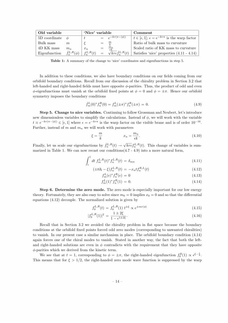
Old variable ‘Nice’ variable Comment5D coordinate φ t = e−kr(π−|φ|) t ∈ [ε, 1]; ε = e−krπ is the warp factorBulk mass m ξ = m

k Ratio of bulk mass to curvature4D KK mass mn xn = mn

εk Scaled ratio of KK mass to curvatureEigenfunction fL,R

n (φ) fL,Rn (t) =

√krεfL,R

n (t) Satisfies ‘nice’ properties (4.11 - 4.14)

Table 1: A summary of the change to ‘nice’ coordinates and eigenfunctions in step 5.

In addition to these conditions, we also have boundary conditions on our fields coming from ourorbifold boundary conditions. Recall from our discussion of the chirality problem in Section 3.2 thatleft-handed and right-handed fields must have opposite φ-parities. Thus, the product of odd and evenφ-eigenfunctions must vanish at the orbifold fixed points at φ = 0 and φ = ±π. Hence our orbifoldsymmetry imposes the boundary conditions

fLm(0)∗fR

n (0) = fLm(±π)∗fR

n (±π) = 0. (4.9)

Step 5. Change to nice variables. Continuing to follow Grossman and Neubert, let’s introducenew dimensionless variables to simplify the calculations. Instead of φ, we will work with the variablet ≡ e−kr(π−|φ|) ∈ [ε, 1] where ε = e−krπ is the warp factor on the visible brane and is of order 10−16.Further, instead of m and mn we will work with parameters

ξ =m

kxn =

mn

εk. (4.10)

Finally, let us scale our eigenfunctions by fL,Rn (t) →

√krεfL,R

n (t). This change of variables is sum-marized in Table 1. We can now recast our conditions(4.7 - 4.9) into a more natural form,

∫ 1

ε

dt fL,Rm (t)∗fL,R

n (t) = δmn (4.11)

(±t∂t − ξ)fL,Rn (t) = −xntfR,L

n (t) (4.12)

fLm(ε)∗fR

n (ε) = 0 (4.13)

fLm(1)∗fR

n (1) = 0. (4.14)

Step 6. Determine the zero mode. The zero mode is especially important for our low energytheory. Fortunately, they are also easy to solve since m0 = 0 implies x0 = 0 and so that the differentialequations (4.12) decouple. The normalized solution is given by

fL,R0 (t) = fL,R

0 (1) t±ξ ∝ e±mr|φ| (4.15)

|fL,R0 (1)|2 =

1± 2ξ

1− ε1±2ξ. (4.16)

Recall that in Section 3.2 we avoided the chirality problem in flat space because the boundaryconditions at the orbifold fixed points forced odd zero modes (corresponding to unwanted chiralities)to vanish. In our present case a similar mechanism in place. The orbifold boundary condition (4.14)again forces one of the chiral modes to vanish. Stated in another way, the fact that both the left-and right-handed solutions are even in φ contradicts with the requirement that they have oppositeφ-parities which we derived from the kinetic term.

We see that at t = 1, corresponding to φ = ±π, the right-handed eigenfunction fR0 (1) ∝ εξ− 1

2 .This means that for ξ > 1/2, the right-handed zero mode wave function is suppressed by the warp

– 14 –

Figure 3: Examples of left- (dashed) and right-handed (solid) eigenmodes fL,Rn with ξ = .45 (left) and

ξ = .55. Boundary conditions are set such that left-handed fields vanish at t = ε, 1. Note that for ξ > 1/2 the

right-handed zero mode fR0 is strongly localized on the hidden brane t = ε. Figure from [8].

factor at the visible brane. This is illustrated in Figure 3, which displays various left- and right-handedeigenmodes for ξ < 1/2 and ξ > 1/2. This is exactly how we will utilize the metric to ‘redshift’ ourneutrino masses in the next section.

Step 7. Determine KK modes. With the zero modes understood we move on to determine thehigher KK excitations. We can combine the equations in (4.12) into a single second-order equation,

[t2∂2

t + x2nt2 − ξ(ξ ∓ 1)

]fL,R

n (t) = 0. (4.17)

The general solutions are Bessel functions, which we can write as9

fL,Rn (t) =

√t[aL,R

n J 12∓ξ(xnt) + bL,R

n J− 12±ξ(xnt)

]. (4.18)

Imposing our original first-order equations (4.12) as constraints, we see that bLn = aR

n and bRn = −aL

n .So our final form for the eigenfunctions are

fLn (t) =

√t[aL

nJ 12−ξ(xnt) + aR

n J− 12+ξ(xnt)

](4.19)

fRn (t) =

√t[aR

n J 12+ξ(xnt) + aL

nJ− 12−ξ(xnt)

]. (4.20)

Next we impose our orbifold boundary conditions (4.13 - 4.14), coming from our requirement that thetwo chiralities have opposite φ-parity. This gives us a discrete KK spectrum. We are free to chooseeither the left-handed modes or the right-handed modes to vanish at the orbifold fixed points t = 0, ε.Since we noted in step 6 that the right-handed zero mode with ξ > 1/2 gave us the warping that wewanted, we shall set fL

n (ε) = fLn (1) = 0.

Our eigenfunctions will be integrated over distributions that are nonsingular in the small parameterε. Thus we can determine the coefficients aL,R

n removing terms that diverge in the limit ε → 0. Wefind that the properly normalized coefficients are aL

n = 0 and |aRn |2 = 2/|J1/2+ξ(xn)|2.

4.3 Generalized see-saw from a bulk neutrino

In the previous section we have developed the complete formalism for a bulk RS1 fermion localizedon the hidden brane. Let us now couple this fermion to the Standard Model to develop a model for

9We are actually making the assumption ξ 6= 12

+ N with N ∈ Z. The special cases where this does not hold lead to

a decomposition in Bessel functions of the first and second kind, but this case is phenomenologically uninteresting.

– 15 –

neutrino mass. This section continues the procedure used by Grossman and Neubert [8]. Our bulkneutrino has lepton number L = 1, so that the only gauge-invariant coupling on the brane is given bya Yukawa term

SH = −∫

d4x√

gvis

{y ¯

0(x)H0(x)ΨR(x, π) + h.c.}

. (4.21)

Here the subscript 0 labels fields that have not yet been canonically normalized with respect to thebrane action. Recall that the lepton doublet `0 is left-handed and has its spinor indices contractedwith the bulk neutrino. Thus ΨL does not couple to the Standard Model since ¯

LΨL = 0. This isespecially nice because in a high energy theory the RS1 branes would have a finite width leading tooverlap with the KK tower of left-handed bulk neutrinos, and hence weak-scale neutrino masses. Letus now canonically normalize our fields as in Section 2.5,

SH = −∑

n≥0

∫d4x

{yn

¯(x)H(x)ψRn (x, ) + h.c.

}, (4.22)

yn =√

ky fRn (1) ≡ zfR

n (1). (4.23)

The second equation defines the effective Yukawa coupling yn to absorb the rescaling of the right-handed neutrino. The combination z ≡

√ky is dimensionless and naturally O(1). After electroweak

symmetry breaking, the uncharged component of the Higgs doublet gets a vacuum expectation valuev and the Yukawa term (4.21) becomes a neutrino mass term ψν

LM ψνR + h.c. in the basis ψν

L =(νL, ψL

1 , · · · , ψLn ) and ψR

ν = (ψR0 , · · · , ψR

n ), with

M =

vy0 vy1 · · · vyn

0 m1 · · · 0... 0

. . . 00 0 · · · mn

. (4.24)

Here n → ∞ and we have included the Dirac mass terms of the bulk neutrino. Recall that for thephenomenologically interesting case ν > 1/2, |vy0| ∼ |fR

0 (1)| ¿ 1 and we get a light neutrino fromparameters that take on natural values.

Physical neutrinos have (mass)2 given by the eigenstates of MM†. Define a unitary matrix U suchthat U†MM†U is diagonal and such that the mass eigenstates ψ

(phys)L are given by ψν

L = U−1ψ(phys)L .

The neutrino mixing angle θν is then defined such that νL = cos θνν(phys)L + · · · , where ν

(phys)L is the

lightest physical neutrino. The mass of the lightest neutrino mν is

mν = v|y0| cos θν (4.25)

= v|zfR0 (1)| cos θν , (4.26)

where we have used (4.23) to write y0 in terms of fR0 (1) and z ∼ O(1). We shall see that experimental

constraints force the mixing angle to be small, so that cos θν ∼ 1. We wrote |fR0 (1)| explicitly in

equation (4.16), from which we have

|fR0 (1)| =

√(2ξ − 1)(1− ε1−2ξ)−1 (4.27)

≈√

2ξ − 1εξ− 12 . (4.28)

Plugging this into equation (4.26), we estimate the lightest neutrino mass to be on the order of

mν ∼ M( v

M

)ξ+ 12

. (4.29)

– 16 –

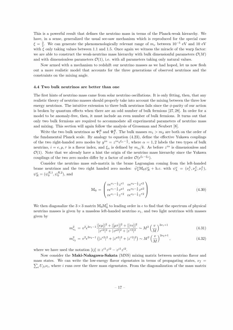
This is a powerful result that defines the neutrino mass in terms of the Planck-weak hierarchy. Wehave, in a sense, generalized the usual see-saw mechanism which is reproduced for the special caseξ = 3

2 . We can generate the phenomenologically relevant range of mν between 10−5 eV and 10 eVwith ξ only taking values between 1.1 and 1.5. Once again we witness the miracle of the warp factor:we are able to construct the weak-neutrino mass hierarchy with bulk dimensionful parameters O(M)and with dimensionless parameters O(1), i.e. with all parameters taking only natural values.

Now armed with a mechanism to redshift our neutrino masses as we had hoped, let us now fleshout a more realistic model that accounts for the three generations of observed neutrinos and theconstraints on the mixing angle.

4.4 Two bulk neutrinos are better than one

The first hints of neutrino mass came from solar neutrino oscillations. It is only fitting, then, that anyrealistic theory of neutrino masses should properly take into account the mixing between the three lowenergy neutrinos. The intuitive extension to three bulk neutrinos fails since the φ-parity of our actionis broken by quantum effects when there are an odd number of bulk fermions [27, 28]. In order for amodel to be anomaly-free, then, it must include an even number of bulk fermions. It turns out thatonly two bulk fermions are required to accommodate all experimental parameters of neutrino massand mixing. This section will again follow the analysis of Grossman and Neubert [8].

Write the two bulk neutrinos as ΨR1 and ΨR

2 . The bulk masses m1 > m2 are both on the order ofthe fundamental Planck scale. By analogy to equation (4.23), define the effective Yukawa couplingsof the two right-handed zero modes by yiα = ziαεξα− 1

2 , where α = 1, 2 labels the two types of bulkneutrino, i = e, µ, τ is a flavor index, and ξα is defined by mα/k. As before ziα is dimensionless andO(1). Note that we already have a hint the origin of the neutrino mass hierarchy since the Yukawacouplings of the two zero modes differ by a factor of order O(εξ1−ξ2).

Consider the neutrino mass sub-matrix in the brane Lagrangian coming from the left-handedbrane neutrinos and the two right handed zero modes: ψν

LM0ψνR + h.c. with ψν

L = (νLe , νL

µ , νLτ ),

ψνR = (ψR,1

0 , ψR,20 ), and

M0 =

vεν1− 12 ze1 vεν2− 1

2 ze2

vεν1− 12 zµ1 vεν2− 1

2 zµ2

vεν1− 12 zτ2 vεν2− 1

2 zτ2

(4.30)

We then diagonalize the 3×3 matrix M0M†0 to leading order in ε to find that the spectrum of physical

neutrino masses is given by a massless left-handed neutrino ν1, and two light neutrinos with massesgiven by

m2v1

= v2ε2ν1−1 |[eµ]|2 + |[µτ ]|2 + |[τe]|2|ze2|2 + |zµ2|2 + |zτ2|2 ∼ M2

( v

M

)2ν1+1

(4.31)

m2v2

= v2ε2ν2−1(|ze2|2 + |zµ2|2 + |zτ2|2) ∼ M2

( v

M

)2ν2+1

, (4.32)

where we have used the notation [ij] ≡ zi1zj2 − zj1zi2.Now consider the Maki-Nakagawa-Sakata (MNS) mixing matrix between neutrino flavor and

mass states. We can write the low-energy flavor eigenstates in terms of propagating states, νf =∑i Ufiνi, where i runs over the three mass eigenstates. From the diagonalization of the mass matrix

– 17 –

Measured Parameter Ref. Constraint Latest Experimental Probetan2 θν = 0.005± 0.003 [34] v0z/k ≤ 0.1 Invisible width of the Z0 at LEP∆m2

21 ∼ 8 · 10−5 eV2 [35] ξ1 ≈ 1.34− 1.37 SNO (solar), KamLAND (reactor)∆m2

32 ∼ 2.4 · 10−3 eV2 [36] ξ2 ≈ 1.27− 1.29 Super Kamiokande (atmospheric)|Ue3|2 > few % [37,38] |ze

2| < |zµ2 |, |zτ

2 | CHOOZ and Super Kamiokandesin2 2θ23 > 0.92 [36] See equation (4.37) Super Kamiokande (atmospheric)sin2 2θ12 = 0.86 [35] See equation (4.38) SNO (solar), KamLAND (reactor)sin2 2θ13 < 0.05 [39] See Table 3 CHOOZ(reactor)

Table 2: Experimental constraints of the Grossman-Neubert model. The results here are updated with the

latest data, summaries are available in [40] and [33].

above and taking the reasonable limit ε → 0, we find

U =

Ue1 Ue2 Ue3

Uµ1 Uµ2 Uµ3

Uτ1 Uτ2 Uτ3

=

[µτ ]∗

N1

zµ∗2 [eµ]−zτ∗

2 [τe]∗

N1N2

ze2

N2[τe]∗

N1

zτ∗2 [µτ ]−ze∗

2 [eµ]∗

N1N2

zµ2

N2[eµ]∗

N1

ze∗2 [τe]−zµ∗

2 [µτ ]∗

N1N2

zτ2

N2

(4.33)

where N21 = |[eµ]|2 + |[µτ ]|2 + |[τe]|2 and N2 = |ze

2|2 + |zµ2 |2 + |zτ

2 |2. Note that each of the ziαs are

O(1), so the elements of U are each order unity. Hence the neutrino mixing matrix lacks the stronghierarchy of the analogous CKM matrix for quarks.

4.5 Realistic phenomenology

Let’s move on to experimental constraints. A summary of relevant experimental constraints is pre-sented in Table 2. Results in this table have been updated to include new data since the originalanalysis in the 1999 Grossman and Neubert paper [8].

There are three types of neutrino mixing data: the flux of solar electron neutrinos compared tothe expected value from hydrogen fusion in the sun, the ratio of muon to electron neutrino flux fromatmospheric neutrinos, and the oscillation of electron antineutrinos from nuclear reactors. Observa-tions are based on detection of characteristic Cerenkov radiation in heavy water. The three sourcesof neutrino data are complimentary and constrain different mixing angles and mass differences. Sincethe publication of Grossman and Neubert’s original paper, the Sudbury Neutrino Observatory andKamLAND reactor experiment have confirmed the large mixing angle MSW model of solar neutrinooscillations [29–33], so we shall disregard other scenarios that Grossman and Neubert also considered.At the end of this essay we briefly mention the current status of low energy sterile neutrinos from theLSND and MiniBooNE collaborations.

First let us consider the neutrino mixing angle between light and heavy modes for a single bulkneutrino in equation (4.26), which is given in terms of the parameters in the mass matrix (4.24) via

tan2 θν =∑

n≥1

v2|yn|2m2

n

=v2|z|2ε2k2

∞∑n=1

2x2

n

=1

2ξ + 1v20z2

k2, (4.34)

where xn are the roots of Jν− 12(xn) = 0. This mixing angle is experimentally constrained to be small

from the measurement of the invisible width of the Z0 boson, which constrains the number of lightneutrinos nν = 2.985±0.008 [34]. If all three light neutrinos contain equal mixings of heavy neutrinos,then nν = 3 cos2 θν , from which we extract the result tan2 θν = 0.005 in table 2. Assuming ξ takes a

– 18 –

natural O(1) value, this value for tan2 θν requires v0z/k ≤ 0.1, which does not require ‘too much’ finetuning. However, natural predictions from bulk RS1 neutrino models are at the edge of experimentalbounds and will be tested by future precision experiments.

Next, let us move on to the ‘realistic’ model with two bulk neutrinos and consider consistencywith the neutrino mass hierarchy. Assuming that the solar and atmospheric neutrino anomalies areexplained by neutrino flavor oscillation, experiments constrain the mass-squared differences ∆m2

ij

between the light neutrinos10. Constraints from solar and atmospheric neutrino data are given intable 2. In our model with two bulk neutrinos, the lightest neutrino is massless. Thus ∆m2

21 = m2ν2

and ∆m232 ' m2

ν3. Using equations (4.31-4.32), we are able to use this to constrain our see-saw

parameters ξ1,2. The key result is that ξ1,2 take natural O(1) values with ξ1,2 > 1/2, as we requiredfor bulk neutrinos localized on the hidden brane.

Finally, consider the low energy MNS matrix U in (4.33). Reactor and atmospheric data limit|Ue3|2 to be on the order of a few percent [37,38], and so |ze

2| should be smaller than |zµ2 | and |zτ

2 |. Inthe limit where |ze

2|2 ¿ |zµ2 |2 + |zτ

2 |2, then the angles θ12 and θ23 satisfy:

sin2 θ12 ' 4|ze1|2(|zµ

2 |2 + |zτ2 |2)|[µτ ]|2

[|ze1|2(|zµ

2 |2 + |zτ2 |2) + |[µτ ]|2]2

(4.35)

sin2 θ23 ' 4|ze2|2|zτ

2 |2(|zµ

2 |2 + |zτ2 |2)2

. (4.36)

The atmospheric anomaly suggests a large νµ ↔ ντ mixing so that sin2 2θ23 > 0.92 [36]. In the limitwhere |ze

2| is much smaller than the other two couplings, this constrains

0.64 < |zµ2 /zτ

2 | < 1.57. (4.37)

Similarly, solar and reactor neutrino data imply sin2 2θ12 = 0.86 [35], implying

|ze1|

|zµ1 zτ

2 − zτ1 zµ

2 |√|zµ

2 |2 + |zτ2 |2 = 0.74. (4.38)

These results are reasonable within the umbrella of naturalness.

5. Lepton Flavor Violation from bulk RS1 neutrinos

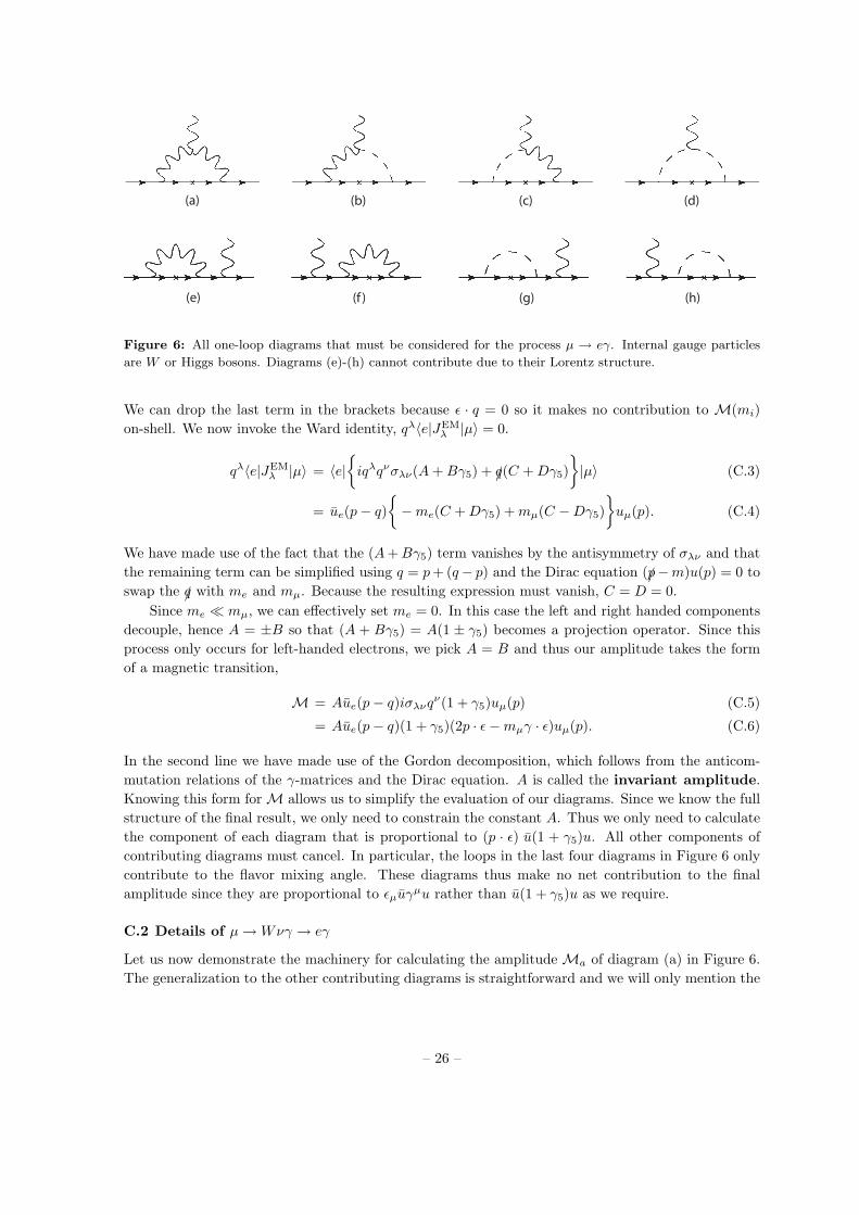
Thus far our RS1 model with bulk neutrinos has agreed nicely with experimental data while main-taining naturalness in its parameters. Theories with massive Dirac neutrinos however, are strictlyconstrained by upper bounds on lepton flavor violating processes. These processes are suppressed wellbelow experimental sensitivity in Standard Model by the GIM mechanism11, but are amplified inextensions to the Standard Model with massive neutrinos [42]. Lepton flavor violating effects for bulkneutrinos in RS1 were first calculated by Ryuichiro Kitano, who showed that the Grossman-Neubertmodel must be finely-tuned in the Higgs sector in order to meet experimental lepton flavor violationconstraints [9]. Kitano calculated the branching ratio of µ → eγ (see Figure 4) and the analogous ra-diative decays of the τ . These decays are given by loop diagrams that are summed over all intermediateKaluza-Klein modes.

– 19 –

Figure 4: Heavy neutrinos violate lepton flavor conservation through radiative decay of charged leptons, such

as µ → eγ. This process is calculated to one-loop order in Appendix C, the result is equation (5.1).

5.1 Radiative charged lepton decay

Kitano’s calculation of µ → eγ in the Grossman-Neubert model is done in more detail in AppendixC. The diagrams that contribute to this process at one loop are shown in Figure 5, where a sum overmassive neutrinos is implied. The result for µ → eγ is given by [9, 10]

M = eg2mµ

(4π)2M2W

( ∞∑

i

U∗µiUeiF

(m2

i

M2W

))ε∗λ(q)ue(p− q)

[iσλρqρ(1 + γ5)

]uµ(p) (5.1)

F (z) =1

12(1− z)4(10− 43z + 78z2 − 49z3 − 18z3 ln z + 4z4

), (5.2)

where i sums over the N th KK mode with N → ∞. Note that Kitano’s published result [9] writesthis formula incorrectly12. F diverges when mi = MW , but we expect the light physical modes tohave mν ¿ MW and the heavy modes to have mi À MW . The asymptotic values for F are given byF (0) = 5/3 and F (∞) = 2/3.

(a) (b) (c) (d)

Figure 5: Diagrams that contribute to the µ → eγ amplitude in equation (5.1). It is implied that one sums

over all neutrino Kaluza-Klein modes in the loop. See Appendix C for more details.

The GIM mechanism suppresses diagrams mediated by light neutrinos mi ¿ MW . However, thissuppression fails in the opposite limit where the Kaluza-Klein excitations are very heavy, mi À MW .In fact, one might be especially concerned because F (∞) 6= 0 and the sum over the KK tower appearsto diverge. In this limit, however, we are saved by the decoupling of very heavy states from low-energy processes, i.e. the fact that physics at very small scales shouldn’t affect physics at much largerscales [45]. Pedagogically this is because processes mediated by a heavy particle are mass suppressedby their propagators. Kitano demonstrates decoupling analytically by looking at the parenthesis in

10By convention we take ∆m2ij = m2

νi−m2

νjwhere mν1 < mν2 < mν3

11In a nutshell, the GIM mechanism describes why flavor changing processes cannot occur at tree level by noting that

such amplitudes are proportional to∑

k UikU∗jk = 0, where U are unitary mixing matrices [41]. Further, such processes

are suppressed at loop level by δm2/M2W , where, in our case, δm = mν .

12Kitano’s equation (20) forgot the power of four in the denominator which is crucial for convergence when summing

over KK modes. He also did not cite Cheng and Li’s calculation in [43,44]. I have e-mailed him regarding these points.

– 20 –

equation 5.1) and setting F (m2i /M

2W ) → F (∞). By using equation (4.34) and MW ∼ gv, one can

approximate the remaining summed term as

g2

M2W

∑

i

UeiU∗µi ≈

∑n

(ze1zµ1

m2n,1

+ze1zµ2

m2n,2

)(5.3)

=1

(kε)2∑

n

(ze1zµ1

1x2

n,1

+ ze2zµ21

x2n,2

)(5.4)

=1

(kε)2

(ze1zµ1

4ξ1 + 2+

ze2zµ2

4ξ2 + 2

). (5.5)

The final line is finite, as promised, though it doesn’t provide much physical intuition about thesource of the decoupling. Cheng and Li followed up Kitano’s calculation by explaining that UeAU∗

µA isproportional to sin2 θA, the mixing of the low energy states with the heavy state A [10]. From (4.34)and experimental limits we see that this mixing gives the desired decoupling sin2 θA ∼ (mν/mA)2.

5.2 Lepton flavor violation phenomenology

Making use of the approximation (5.5), decay width for radiative muon decay is given by

Γ(µ → eγ) =e2m5

µ

4(4π)5(εk)4

∣∣∣∣ze1zµ1

4ξ1 + 2+

ze2zµ2

4ξ2 + 2

∣∣∣∣2

(5.6)

= 0.0037( v

εk

)2∣∣∣∣ze1zµ1

4ξ1 + 2+

ze2zµ2

4ξ2 + 2

∣∣∣∣2

. (5.7)

The analogous τ decays are given by making the replacements µ → τ , e → µ, e and 0.0037 → 0.00065.The LAMPF-MEGA and CLEO experiments bound the branching ratios of these decays to be [46–48]

Br(µ → eγ) < 1.2× 10−11 (5.8)

Br(τ → µγ) < 1.1× 10−6 (5.9)

Br(τ → eγ) < 2.7× 10−6. (5.10)

Thus, using the fact that z and ξ are O(1), one can constrain

v

εk> 0.02. (5.11)

Applying relation (4.10), this gives us a bound on the lowest Kaluza-Klein mass,

mKK ? 25 TeV. (5.12)

This is two orders of magnitude greater than the Higgs vacuum expectation value, so a fine tuningon the order of 10−2 is necessary. We can go a bit further with this and recast the constraints on themixing angles in table 2 in terms of the O(1) Yukawa parameters using (4.34). We first employ theapproximate relations between dimensionless Yukawa couplings

|ze1| ∼ 0.7|zµ

1 | ∼ 0.7|zτ1 |. (5.13)

Using this, Grossman and Neubert computed more stringent constraints on the Yukawa couplings,presented in table 3. These couplings are also pushing the limits of what one might consider natural.

– 21 –

Family index, i Bulk index, α Constraint on |ziα| Conditions

e, µ, τ 1 > 0.02 Large angle MSW solutione 2 > 0.009 Taking sin2 2θ13 = 0.05 [39]

µ, τ 2 > 0.05 Taking sin2 2θ13 = 0.05 [39]

Table 3: Constraints on the effective dimensionless Yukawa couplings |ziα| from the µ → eγ branching ratio

and the mixing angle constraints in table 2.

6. Summary and further directions

In this essay we have introduced the RS1 model and the Grossman-Neubert minimal extension withbulk fermions to explain neutrino masses and mixings. This extension is able to use the RS1 warp factorto generate the neutrino-weak hierarchy and the hierarchy between neutrino masses via a generalizedsee-saw mechanism with only natural parameters. We then focused on experimental constraints fromlepton flavor violation in charged lepton decay. This process was able to strictly constrain the lowestKK mass and Yukawa couplings of the bulk neutrino, but it forced the minimal model into a cornerby requiring levels of fine-tuning. The next source of precision data in the lepton sector would comefrom the proposed International Linear Collider (ILC), which will further probe lepton flavor violatingprocesses [49].

Until then, the model discussed in this essay lends itself to further directions of research. Theformalism developed for bulk RS1 neutrinos is general and can be applied to other fermionic particles.In particular, Gherghetta and Pomarol have proposed a supersymmetric RS1 where all fields are freeto propagate in the bulk [50]. During the course of this writing [51] appeared. It studies µ → eγ decayswith a bulk Standard Model and two Higgs doublets. One can go further and place all sorts of StandardModel extensions into the bulk, such as technicolor. Because of its strong suppression in the StandardModel and sensitivity to particles that couple to leptons and the W boson, lepton flavor violation is astrong experimental check for physics beyond the Standard Model. Like many signals, unfortunately,it is difficult to disambiguate between models of extra dimensions and supersymmetry [52] (or evenmore exotic models).

One can also continue from the work presented here in one of many orthogonal directions. A recentconstraint on particle physics models comes from early universe cosmology. Studies of the cosmologyof warped extra dimensions [53] can be used in conjunction with dark matter densities to constrainthe relic density of undiscovered heavy particles. In another direction, the general flavor structure ofmodels with a warped extra dimension have only recently been studied [54]. To the best of this author’sknowledge, there is yet no published analysis of CP violation in the Grossman-Neubert model. Thismay be an interesting topic to study that may yield some insight on CP violation beyond the StandardModel. Yet another direction involves recent attempts in bottom-up neutrino model-building by Maand his collaborators. Ma has proposed of a discrete A4 family symmetry which seems to approximateobserved neutrino mixing results [55]. One might attempt to connect the theoretical prediction of RS1bulk neutrino mixing to this A4 family symmetry or, conversely, use the A4 symmetry to motivatenon-minimal bulk neutrino extensions to RS1. Again, to the best of this author’s knowledge, there isyet no published analysis of the compatibility of the Grossman-Neubert model with such bottom-uppredictions.

Finally, the Grossman-Neubert model with two bulk neutrinos would have to be extended to atleast four neutrinos if the lightest neutrino is found to have nonzero mass. This, however, would naively

– 22 –

suggest the existence of a light sterile neutrino. Recent results from the MiniBooNE collaboration,however, appear to refute LSND results that suggested the existence of such a particle [56]. Toclose, I offer a quote from the anonymous CERN blog Resonaances13 regarding the possibility ofaccommodating both LSND and MiniBooNE data within an extra dimensional model: “By shapingthe extra dimensions properly, the model can accommodate the MiniBooNE excess at lower energies aswell as the suppression of oscillations at higher energies. My impression is that, with a little bit morework, the model could accommodate Harry Potter, too.”

7. Acknowledgements

I would like to thank Ben Allanach for his time guiding this essay and for many illuminating conversa-tions on particle phenomenology. I credit Matthew Reece for connecting the 5D chirality problem withthe sign the bulk fermion mass term. After the writing of this essay Matthias Neubert also offeredhis thoughts on the chirality problem in a personal communication. LATEX typesetting was done usingMiKTeX 2.5, Latex Editor (LEd), and Jaxodraw [57]. I would like to thank my fellow students SteffenGielen, Leo van-Nierop, and David Simmons-Duffin for letting me bounce ideas off them while brain-storming for this essay. Additional thanks to Steffen Gielen for proof reading my essay for spellingand grammar. Finally, I would like to dedicate this work to all of my Part III friends from whom Ihave learned so much and whose shared passion for physics (and late night table football) has madePart III a very special experience.

A. Notation and Convention

There is no globally accepted standard for conventions when dealing with extra dimensions. I will tryto minimize the redefinition of common notation. The effective 4D Planck scale is denoted by the usualMPl while the fundamental 5D Planck scale is M . Bulk coordinates are indexed with capital Romanletters from the middle of the alphabet, M,N ∈ {0, · · · , 4}. We parameterize the extra dimension x5

by an angular coordinate, φ, with an associated radius of compactification r. Cartesian coordinateson the 3-brane are given by the usual lowercase Greek letters, µ, ν ∈ {0, · · · , 3}. The bulk metric isdenoted by gMN and the 3-brane metric denoted by (gvis)µν .

When dealing with fermions it is necessary to work with a little more formalism and distinguishbetween the manifold and its tangent space. We shall reserve capital Roman letters (A,B) at thebeginning of the alphabet to index the bulk tangent space. The bulk vielbein is given by eA

M . Theinverse vielbein is denoted with flipped indices, eM

A . We will take the Minkowski metric to be ‘mostlyminus’,

ηAB = diag(+,−,−,−,−) (A.1)

ηαβ = diag(+,−,−,−) (A.2)

In the interests of readability, I have taken the liberty of using different variables relative to some ofthe main works cited. As a final point of convention, I apologize for adopting American English andfor its brutalization of ‘proper’ spelling.

13http://resonaances.blogspot.com/2007/04/after-miniboone.html

– 23 –

B. Properties of the RS1 bulk eigenbasis

Here we derive the orthogonality relation (4.7) and differential equation (4.8) for the f(φ) eigenbasisof the RS1 orbifold direction. These follow from demanding that integrating out φ in the bulk actiongives us the effective action. Recall that the bulk action takes the form (4.4):

Sf =∫

d4x

∫dφ r

{e−3σ

(ΨLi/∂ΨL + ΨRi/∂ΨR

)− e−4σm · sgn(φ)(ΨLΨR + ΨRΨL

)

− 12r

[ΨL

(e−4σ∂φ + ∂φe−4σ

)ΨR − ΨR

(e−4σ∂φ + ∂φe−4σ

)ΨL

] }. (B.1)

We compare this to the effective action for the Kaluza-Klein tower (4.6):

S(4D)f =

∑n

∫d4x

{ψn(x)i/∂ψn(x)−mnψn(x)ψn(x)

}, (B.2)

Finally, recall that the our Kaluza-Klein decomposition is (4.5):

ΨL,R(x, φ) =∑

n

ψL,Rn (x)

e2σ

√rfL,R

n (φ). (B.3)

B.1 Orthogonality

The 4D derivative terms should give us that corresponding kinetic terms in the effective theory.Looking at the left handed components of the these terms, we get

r{e−eσ

(ψL i/∂ ψL

)}= re−eσ

{(∑n

ψLn

e2σ

√rfL∗

n

)i/∂

(∑m

ψLn

e2σ

√rfL

n

)}(B.4)

= re−3σ∑n,m

(e4σ

rfL∗

n fLm ψL

n i/∂ ψLn

)(B.5)

= eσ fL∗n fL

m (B.6)

The right handed part is the same with L → R. Integrating and comparing to the kinetic term of(4.6), we see that we get the orthnormality condition (4.7),

∫dφ eσ(fL,R

n )∗fL,Rm = δmn. (B.7)

B.2 Differential Equation for f

Now consider the remaining terms in the bulk action (4.4). These are (anti)symmetric with respect to(L ↔ R), so it is sufficient to work with terms of only one chirality. Because of the orbifold symmetryit is sufficient to assume φ > 0. First consider the term coming from the φ-component of the 5D

– 24 –

kinetic part of the Lagrangian:

−12ΨL

{e−4σ, ∂φ

}ΨR = −

∑m,n

12(ψL

n

e2σ

√rfL∗

n )(e−4σ∂φ + ∂φe−4σ)(ψRm

e2σ

√rfR∗

m ) (B.8)

= −∑m,n

12r

ψLn

{e2σ fL∗

n (e−4σ∂φ + ∂φe−4σ)e2σ fR∗m

}ψR

m (B.9)

= −∑m,n

12r

ψLn e2σ fL∗

n

{e−4σ(2

∂σ

∂φ+ f ′Rm ) + (−∂σ

∂φ+ f ′Rm )

}e2σψR

m (B.10)

= −∑m,n

ψLnψR

m fL∗n (

1r∂φ)fR

m. (B.11)

Note that corresponding term with L ↔ R has a relative sign. Moving on to the bulk mass term,

−m re−4σΨLΨR = −∑m,n

m re−4σ

(ψL

n

e2σ

√rfL∗

n

)(ψR

m

e2σ

√rfR

m

)(B.12)

= −m ψLnψR

m fL∗n fR

m. (B.13)

Combining (B.11) and (B.13) and setting equal to the 4D mass term in the effective theory, we have

−∑

n

mn ψnψn = −∑m,n

∫dφ

{[ψL

nψRm fL∗

n (1r∂φ)fR

m − (L ↔ R)]

−[mψL

nψRm fL∗

n fRm + (L ↔ R)

]}(B.14)

By using the orthogonality relation (B.7) and combining chiral spinors into Dirac spinors, we finallyget the desired differential equation (4.8) for the f ’s,

(±1

r∂φ −m

)ˆfL,R

n (φ) = −mneσ fR,Ln (φ). (B.15)

C. Highlights of the calculation µ → eγ in RS1 with bulk neutrinos

Here we derive the result (5.1) for the radiative decay µ → eγ. The result is given by

M =∑

i

M(mi), (C.1)

where M(mi) is the amplitude mediated by a neutrino of mass mi. It is sufficient, then, to calculate ageneral M(mi), which we will henceforth refer to as M to simplify notation. We provide some detailsfollowing the texts by Cheng and Li [43,44]. I have chosen to highlight some details of the calculationnot made explicit in the texts.

C.1 Lorentz structure

Let us begin with the Lorentz structure of the amplitude, M = ελ〈e|JEMλ |µ〉. We can expand the

bra-ket into the following basis of 4× 4 matrices,

〈e|JEMλ |µ〉 = ue(p− q)

{iqνσλν(A + Bγ5) + γλ(C + Dγ5) + qλ(E + Fγ5)

}uµ(p). (C.2)

– 25 –

(a) (b) (c) (d)

(e) (f ) (g) (h)

Figure 6: All one-loop diagrams that must be considered for the process µ → eγ. Internal gauge particles

are W or Higgs bosons. Diagrams (e)-(h) cannot contribute due to their Lorentz structure.

We can drop the last term in the brackets because ε · q = 0 so it makes no contribution to M(mi)on-shell. We now invoke the Ward identity, qλ〈e|JEM

λ |µ〉 = 0.

qλ〈e|JEMλ |µ〉 = 〈e|

{iqλqνσλν(A + Bγ5) + /q(C + Dγ5)

}|µ〉 (C.3)

= ue(p− q){−me(C + Dγ5) + mµ(C −Dγ5)

}uµ(p). (C.4)

We have made use of the fact that the (A + Bγ5) term vanishes by the antisymmetry of σλν and thatthe remaining term can be simplified using q = p + (q− p) and the Dirac equation (/p−m)u(p) = 0 toswap the /q with me and mµ. Because the resulting expression must vanish, C = D = 0.

Since me ¿ mµ, we can effectively set me = 0. In this case the left and right handed componentsdecouple, hence A = ±B so that (A + Bγ5) = A(1 ± γ5) becomes a projection operator. Since thisprocess only occurs for left-handed electrons, we pick A = B and thus our amplitude takes the formof a magnetic transition,

M = Aue(p− q)iσλνqν(1 + γ5)uµ(p) (C.5)

= Aue(p− q)(1 + γ5)(2p · ε−mµγ · ε)uµ(p). (C.6)

In the second line we have made use of the Gordon decomposition, which follows from the anticom-mutation relations of the γ-matrices and the Dirac equation. A is called the invariant amplitude.Knowing this form for M allows us to simplify the evaluation of our diagrams. Since we know the fullstructure of the final result, we only need to constrain the constant A. Thus we only need to calculatethe component of each diagram that is proportional to (p · ε) u(1 + γ5)u. All other components ofcontributing diagrams must cancel. In particular, the loops in the last four diagrams in Figure 6 onlycontribute to the flavor mixing angle. These diagrams thus make no net contribution to the finalamplitude since they are proportional to εµuγµu rather than u(1 + γ5)u as we require.

C.2 Details of µ → Wνγ → eγ

Let us now demonstrate the machinery for calculating the amplitude Ma of diagram (a) in Figure 6.The generalization to the other contributing diagrams is straightforward and we will only mention the

– 26 –

p (p+k)

q

(p-q)

(k+q)k

Figure 7: The assignment of momenta for the calculation of µ → eγ.

results of those analogous calculations. The assignment of momentum variables is shown in Figure 7.Applying the Feynman rules in ’t Hooft-Feynman gauge,

Ma = −i∑

i

∫d4x

(2π)4ue(p− q)

(ig

2√

2

)U∗

eiγµ(1− γ5)i

(/p + /k)−mi

(ig

2√

2

)

× Uµiγν(1− γ5)uµ(p)−igνβ

k2 −M2W

−igµα

(k + q)2 −M2W

(−ieΓαβ) (C.7)

Γαβ = (2k · ε)gαβ − (k + 2q)βεα − (k − q)νεβ (C.8)

Where Γ contains the WWγ vertex and the photon polarization. We can simplify this by writing thespin contraction as Nµν ,

Ma = −ig2e

4

∑

i

U∗eiUµi

∫d4k

(2π)4NµνΓµν

[(p + k)2 −m2i ][k2 −M2

W ][(k + q)2 −M2W ]

(C.9)

Nµν = ue(p− q)γµ(/p + /k)γν(1− γ5)uµ(p). (C.10)

The natural step is to introduce Feynman parameters to combine the denominators. For our case therelevant expression is

1A1

1A2

1A3

= 2!∫ 1

0

dα1 dα2 δ(1− α1 − α2)[α1A1 + α2A2 + (1− α1 − α2)A3]

3 (C.11)

(C.12)

where the Ai are given by the denominators in (C.9). One finds that

α1A1 + α2A2 + (1− α1α2)A3 = (k + α1p + α2q)2 − (1− α1)M2W − α1m

2i ), (C.13)

and hence the denominator becomes ‘nice’ with respect to the momentum integral if we make theshift k = ` + α1p + α2q. Now recall that our goal is to determine the components of this amplitudeproportional to (p · ε) u(1 + γ5)u. Inserting this shift into the numerator NµνΓµν we can isolate theterms proportional to p · ε to get

NµνΓµν = (p · ε)[u(1 + γ5)uµ] 2mµ[2(1− α1)2 + (2α1 − 1)α2] + · · · . (C.14)

Dropping the other terms (which end up canceling, as argued above), we can now perform the mo-mentum integration

∫d4`

(2π)41

(`2 − a2)3=

i

32π2a2, (C.15)

– 27 –

where a2 = (1−α1)M2W +α1m

2i . Plugging all of this into (C.9) and reading off the ‘invariant amplitude’

A from (C.6), we have

Aa = g2e∑

i

U∗eiUµi(p · ε)[u(1 + γ5)uµ]

∫ 1

0

dα1 dα2mµ[2(1− α1)2 + (2α1 − 1)α2]32π2 [(1− α1)M2

W + α1m2i ]

(C.16)

=∑

i

cimµ

16π2

1M2

W

∫ 1

0

dα1

(1− α1)2( 32 − α1)

[(1− α1) + α1(m2i /M

2W )]

, (C.17)

where we’ve written ci = 14g2eU∗

eiUµi.

C.3 Results for the remaining diagrams

One can now perform the calculations for the remaining diagrams. The machinery is completelyanalogous: combine the denominator with Feynman parameters, shift the momentum variable, andthen isolate the terms proportional to (p · ε) in the numerator. One can then perform the momentumand α2 integral for these terms. Summing these all together one gets the result (5.1),

M(mi) =mµ

M2W

∑

i

ci F (m2

i

M2W

) ue(p− q)iσλνqν(1 + γ5)uµ(p) (C.18)

F (z) =∫ 1

0

dα(1− α)

(1− α) + αz[2(1− α)(2− α) + α(1 + α)z]. (C.19)

The expression for F (z) can be integrated explicitly. This is done in [44] or easily in Mathematica(there’s no physics to be extracted from this calculation). One ends up with the explicit form in (5.2):F (z) =

(10− 43z + 78z2 − 49z3 − 18z3 ln z + 4z4

)/(12(1− z)4).

One might be concerned that the other diagrams differ by replacing one or both W propagatorswith Higgs propagators, and hence it’s not clear that the terms in the invariant amplitudes are allproportional to e g2mµ/M2

W . However, one can write out the Higgs propagator and couplings tovarious particles in terms of MW and we end up with the correct factors as one might be able to guessfrom dimensional arguments.

References

[1] N. Arkani-Hamed, S. Dimopoulos, and G. R. Dvali, The hierarchy problem and new dimensions at a

millimeter, Phys. Lett. B429 (1998) 263–272, [hep-ph/9803315].

[2] L. Randall and R. Sundrum, A large mass hierarchy from a small extra dimension, Phys. Rev. Lett. 83

(1999) 3370–3373, [hep-ph/9905221].

[3] K. Akama, An early proposal of ’brane world’, Lect. Notes Phys. 176 (1982) 267–271, [hep-th/0001113].

[4] V. A. Rubakov and M. E. Shaposhnikov, Do we live inside a domain wall?, Phys. Lett. B125 (1983)

136–138.

[5] Super-Kamiokande Collaboration, Y. Ashie et al., Evidence for an oscillatory signature in

atmospheric neutrino oscillation, Phys. Rev. Lett. 93 (2004) 101801, [hep-ex/0404034].

[6] M. Jezabek and Y. Sumino, Neutrino mixing and seesaw mechanism, Phys. Lett. B440 (1998) 327–331,

[hep-ph/9807310].

[7] N. Arkani-Hamed, S. Dimopoulos, G. R. Dvali, and J. March-Russell, Neutrino masses from large extra

dimensions, Phys. Rev. D65 (2002) 024032, [hep-ph/9811448].

– 28 –

[8] Y. Grossman and M. Neubert, Neutrino masses and mixings in non-factorizable geometry, Phys. Lett.

B474 (2000) 361–371, [hep-ph/9912408].

[9] R. Kitano, Lepton flavor violation in the randall-sundrum model with bulk neutrinos, Phys. Lett. B481

(2000) 39–44, [hep-ph/0002279].

[10] T. P. Cheng and L.-F. Li, Heavy particle electroweak loop effects in extra- dimensional models with bulk

neutrinos, Phys. Lett. B502 (2001) 152–158, [hep-ph/0101068].

[11] R. Sundrum, Effective field theory for a three-brane universe, Phys. Rev. D59 (1999) 085009,

[hep-ph/9805471].

[12] P. Horava and E. Witten, Heterotic and type i string dynamics from eleven dimensions, Nucl. Phys.

B460 (1996) 506–524, [hep-th/9510209].

[13] E. Witten, Strong coupling expansion of calabi-yau compactification, Nucl. Phys. B471 (1996) 135–158,

[hep-th/9602070].

[14] R. Rattazzi, Cargese lectures on extra dimensions, hep-ph/0607055.

[15] H. Haber and A. E. Nelson, Particle Physics And Cosmology: The Quest For Physics Beyond The

Standard Model(s): TASI 2002. World Scientific, USA (2004).

[16] R. Sundrum, To the fifth dimension and back. (tasi 2004), hep-th/0508134.

[17] S. P. Robinson, Normalization conventions for newton’s constant and the planck scale in arbitrary

spacetime dimension, gr-qc/0609060.

[18] C. Csaki, Tasi lectures on extra dimensions and branes, hep-ph/0404096.

[19] R. Wald, General Relativity. Chicago University Press. (1984).

[20] W. D. Goldberger and M. B. Wise, Modulus stabilization with bulk fields, Phys. Rev. Lett. 83 (1999)

4922–4925, [hep-ph/9907447].

[21] J. M. Maldacena, Lectures on ads/cft, hep-th/0309246.

[22] N. Arkani-Hamed, M. Porrati, and L. Randall, Holography and phenomenology, JHEP 08 (2001) 017,

[hep-th/0012148].

[23] R. Rattazzi and A. Zaffaroni, Comments on the holographic picture of the randall-sundrum model, JHEP

04 (2001) 021, [hep-th/0012248].

[24] H. Davoudiasl, J. L. Hewett, and T. G. Rizzo, Phenomenology of the randall-sundrum gauge hierarchy

model, Phys. Rev. Lett. 84 (2000) 2080, [hep-ph/9909255].

[25] R. A. Bertlmann, Anomalies in Quantum Field Theory. Oxford, UK: Oxford University Press (1996).

[26] H. Murayama, Notes on clifford algebra and spin(n) representations, . Lecture notes from Physics 230A

(Spring 2007), University of California Berkeley. http://hitoshi.berkeley.edu/230A/clifford.pdf.

[27] A. N. Redlich, Gauge noninvariance and parity nonconservation of three- dimensional fermions, Phys.

Rev. Lett. 52 (1984) 18.

[28] J. Callan, Curtis G. and J. A. Harvey, Anomalies and fermion zero modes on strings and domain walls,

Nucl. Phys. B250 (1985) 427.

[29] S. P. Mikheev and A. Y. Smirnov, Resonance enhancement of oscillations in matter and solar neutrino

spectroscopy, Sov. J. Nucl. Phys. 42 (1985) 913–917.

[30] L. Wolfenstein, Neutrino oscillations in matter, Phys. Rev. D17 (1978) 2369.

[31] SNO Collaboration, Q. R. Ahmad et al., Measurement of day and night neutrino energy spectra at sno

and constraints on neutrino mixing parameters, Phys. Rev. Lett. 89 (2002) 011302, [nucl-ex/0204009].

[32] P. C. de Holanda and A. Y. Smirnov, Lma msw solution of the solar neutrino problem and first kamland

results, JCAP 0302 (2003) 001, [hep-ph/0212270].

– 29 –

[33] W.-M. Yao, C. Amsler, D. Asner, R. Barnett, J. Beringer, P. Burchat, C. Carone, C. Caso, O. Dahl,

G. D’Ambrosio, A. DeGouvea, M. Doser, S. Eidelman, J. Feng, T. Gherghetta, M. Goodman, C. Grab,

D. Groom, A. Gurtu, K. Hagiwara, K. Hayes, J. Hernandez-Rey, K. Hikasa, H. Jawahery, C. Kolda,

K. Y., M. Mangano, A. Manohar, A. Masoni, R. Miquel, K. Monig, H. Murayama, K. Nakamura,

S. Navas, K. Olive, L. Pape, C. Patrignani, A. Piepke, G. Punzi, G. Raffelt, J. Smith, M. Tanabashi,

J. Terning, N. Tornqvist, T. Trippe, P. Vogel, T. Watari, C. Wohl, R. Workman, P. Zyla, B. Armstrong,

G. Harper, V. Lugovsky, P. Schaffner, M. Artuso, K. Babu, H. Band, E. Barberio, M. Battaglia,

H. Bichsel, O. Biebel, P. Bloch, E. Blucher, R. Cahn, D. Casper, A. Cattai, A. Ceccucci,

D. Chakraborty, R. Chivukula, G. Cowan, T. Damour, T. DeGrand, K. Desler, M. Dobbs, M. Drees,

A. Edwards, D. Edwards, V. Elvira, J. Erler, V. Ezhela, W. Fetscher, B. Fields, B. Foster,

D. Froidevaux, T. Gaisser, L. Garren, H.-J. Gerber, G. Gerbier, L. Gibbons, F. Gilman, G. Giudice,

A. Gritsan, M. Grunewald, H. Haber, C. Hagmann, I. Hinchliffe, A. Hocker, P. Igo-Kemenes, J. Jackson,

K. Johnson, D. Karlen, B. Kayser, D. Kirkby, S. Klein, K. Kleinknecht, I. Knowles, R. Kowalewski,

P. Kreitz, B. Krusche, Y. Kuyanov, O. Lahav, P. Langacker, A. Liddle, Z. Ligeti, T. Liss, L. Littenberg,

L. Liu, K. Lugovsky, S. Lugovsky, T. Mannel, D. Manley, W. Marciano, A. Martin, D. Milstead,

M. Narain, P. Nason, Y. Nir, J. Peacock, S. Prell, A. Quadt, S. Raby, B. Ratcliff, E. Razuvaev, B. Renk,

P. Richardson, S. Roesler, G. Rolandi, M. Ronan, L. Rosenberg, C. Sachrajda, S. Sarkar, M. Schmitt,

O. Schneider, D. Scott, T. Sjostrand, G. Smoot, P. Sokolsky, S. Spanier, H. Spieler, A. Stahl, T. Stanev,

R. Streitmatter, T. Sumiyoshi, N. Tkachenko, G. Trilling, G. Valencia, K. van Bibber, M. Vincter,

D. Ward, B. Webber, J. Wells, M. Whalley, L. Wolfenstein, J. Womersley, C. Woody, A. Yamamoto,

O. Zenin, J. Zhang, and R.-Y. Zhu, Review of Particle Physics, Journal of Physics G 33 (2006) 1+.

[34] A. Sirlin, Ten years of precision electroweak physics, hep-ph/9912227.

[35] SNO Collaboration, B. Aharmim et al., Electron energy spectra, fluxes, and day-night asymmetries of

b-8 solar neutrinos from the 391-day salt phase sno data set, Phys. Rev. C72 (2005) 055502,

[nucl-ex/0502021].

[36] Super-Kamiokande Collaboration, Y. Ashie et al., Evidence for an oscillatory signature in

atmospheric neutrino oscillation, Phys. Rev. Lett. 93 (2004) 101801, [hep-ex/0404034].

[37] CHOOZ Collaboration, M. Apollonio et al., Limits on neutrino oscillations from the chooz experiment,

Phys. Lett. B466 (1999) 415–430, [hep-ex/9907037].

[38] G. L. Fogli, E. Lisi, A. Marrone, and G. Scioscia, Super-kamiokande atmospheric neutrino data, zenith

distributions, and three-flavor oscillations, Phys. Rev. D59 (1999) 033001, [hep-ph/9808205].

[39] Chooz Collaboration, C. Bemporad, Results from chooz, Nucl. Phys. Proc. Suppl. 77 (1999) 159–165.

[40] A. Strumia and F. Vissani, Implications of neutrino data circa 2005, Nucl. Phys. B726 (2005) 294–316,

[hep-ph/0503246].

[41] S. L. Glashow, J. Iliopoulos, and L. Maiani, Weak interactions with lepton-hadron symmetry, Phys. Rev.

D2 (1970) 1285–1292.

[42] T. P. Cheng and L.-F. Li, mu → e gamma in theories with dirac and majorana neutrino mass terms,

Phys. Rev. Lett. 45 (1980) 1908.

[43] T.-P. Cheng and L.-F. Li, Gauge theory of elementary particle physics. Clarendon Press. (1984) Section

13.3.

[44] T.-P. Cheng and L.-F. Li, Gauge Theory of Elementary Particle Physics: Problems and Solutions.

Clarendon Press. (2000) Section 13.4.

[45] T. P. Cheng and L.-F. Li, Effects of superheavy neutrinos in low-energy weak processes, Phys. Rev. D44

(1991) 1502–1509.

[46] MEGA Collaboration, M. L. Brooks et al., New limit for the family-number non-conserving decay mu+

– ¿ e+ gamma, Phys. Rev. Lett. 83 (1999) 1521–1524, [hep-ex/9905013].

– 30 –

[47] CLEO Collaboration, S. Ahmed et al., Update of the search for the neutrinoless decay tau –¿ mu

gamma, Phys. Rev. D61 (2000) 071101, [hep-ex/9910060].

[48] CLEO Collaboration, K. W. Edwards et al., Search for neutrinoless tau decays: tau –¿ e gamma and

tau –¿ mu gamma, Phys. Rev. D55 (1997) 3919–3923.

[49] N. Arkani-Hamed, H.-C. Cheng, J. L. Feng, and L. J. Hall, Probing lepton flavor violation at future

colliders, Phys. Rev. Lett. 77 (Sep, 1996) 1937–1940.

[50] T. Gherghetta and A. Pomarol, Bulk fields and supersymmetry in a slice of ads, Nucl. Phys. B586

(2000) 141–162, [hep-ph/0003129].

[51] E. O. Iltan, Radiative lepton flavor violating decays in the randall sundrum background with localized

leptons, arXiv:0704.4000 [hep-ph].

[52] H.-C. Cheng, K. T. Matchev, and M. Schmaltz, Bosonic supersymmetry? getting fooled at the lhc,

Physical Review D 66 (2002) 056006.

[53] C. Csaki, M. Graesser, C. F. Kolda, and J. Terning, Cosmology of one extra dimension with localized

gravity, Phys. Lett. B462 (1999) 34–40, [hep-ph/9906513].

[54] K. Agashe, G. Perez, and A. Soni, Flavor structure of warped extra dimension models, Phys. Rev. D71

(2005) 016002, [hep-ph/0408134].

[55] E. Ma and G. Rajasekaran, Softly broken a 4 symmetry for nearly degenerate neutrino masses, Physical

Review D 64 (2001) 113012.

[56] The MiniBooNE Collaboration, A. A. Aguilar-Arevalo et al., A search for electron neutrino

appearance at the δm2 ∼ 1 ev2 scale, arXiv:0704.1500 [hep-ex].

[57] D. Binosi and L. Theussl, Jaxodraw: A graphical user interface for drawing feynman diagrams, Comput.

Phys. Commun. 161 (2004) 76–86, [hep-ph/0309015].

– 31 –