master thesis - dlr portalelib.dlr.de/114051/1/master thesis report_sangram.pdfmaster thesis...

MASTER THESIS

‘’ACCELERATED STRESS TESTING PROTOCOLS OF PROTON EXCHANGE MEMBRANE

(PEM) ELECTROLYZERS’’

by

Sangram Ashok Savant

submitted in partial fulfillment for degree of

Master of Science in ‘Energy Engineering and Management’

conducted at

KIT Supervisors

DLR Supervisors

Prof. Dr. rer. nat Helmut Ehrenberg MSc. Julio César García Navarro Dr. Frieder Scheiba Dr. Indro Biswas Prof. Dr.-Ing Mathias Noe

i

ॐ असतो मा सदगमय ।

तमसो मा जयोततगगमय ।

मतयोमाग अमत गमय । ॐ शानतिः शानतिः शानतिः ॥

Om Asato Maa Sad-Gamaya |

Tamaso Maa Jyotir-Gamaya |

Mrtyor-Maa Amrtam Gamaya |

Om Shaantih Shaantih Shaantih ||

Keep us not in the Unreality (of the bondage of the Phenomenal World), but lead us towards

the Reality (of the Eternal Self),

Keep us not in the Darkness (of Ignorance), but lead us towards the Light (of Knowledge),

Keep us not in the Fear of Death (due to the bondage to the Mortal World), but lead us

towards the Immortality (gained by the Knowledge and performing Dharma),

Om, (May there be) Peace, Peace, Peace.

- Bṛhadāraṇyaka Upaniṣad (Ancient Indian Treatise)

https://en.wikipedia.org/wiki/B%E1%B9%9Bhad%C4%81ra%E1%B9%87yaka_Upani%E1%B9%A3ad

ii

Name: Sangram Ashok Savant

Date & Place of Birth: 02/11/1992, Sangli, India.

Matriculation N°: 1950409

Declaration of Sangram Ashok Savant

I declare that I prepared this Master Thesis on my own without any external help or assistance.

Used literature and internet sources are completely listed in the appendix of this work. I assure

to have marked everything what has been taken from the work of third parties.

Karlsruhe, September 6, 2017 ___________________________ (Sangram Ashok Savant)

iii

CONTENTS

LIST OF FIGURES................................................................................................................................................................ v

LIST OF TABLES ................................................................................................................................................................ vi

LIST OF GRAPHS...............................................................................................................................................................vii

PREFACE ............................................................................................................................................................................... ix

ABSTRACT ............................................................................................................................................................................ 1

1 INTRODUCTION ........................................................................................................................................................ 2

1.1 HYDROGEN PRODUCTION AND APPLICATION ................................................................................. 4

1.2 ELECTROLYSIS ................................................................................................................................................ 6

1.3 THERMODYNAMICS ...................................................................................................................................... 7

2 OVERVIEW OF WATER ELECTROLYSIS TECHNOLOGIES ....................................................................... 9

2.1 ALKALINE WATER ELECTROLYZERS ................................................................................................. 10

2.2 PROTON EXCHANGE MEMBRANE (PEM) ELECTROLYZERS .................................................... 13

2.3 SOLID OXIDE ELECTROLYTE ELECTROLYZERS............................................................................. 17

3 TEST BENCH ............................................................................................................................................................ 19

3.1 COMPONENT SUMMARY OF THE TEST BENCH ............................................................................. 19

3.2 EXPLODED VIEW OF THE ELECTROLYZER...................................................................................... 21

4 LOSSES IN A PEM ELECTROLYZER ................................................................................................................ 23

4.1 OPEN CIRCUIT VOLTAGE ......................................................................................................................... 23

4.2 OHMIC OVERPOTENTIAL/LOSSES ...................................................................................................... 23

4.3 ACTIVATION OVERPOTENTIAL/LOSSES .......................................................................................... 24

4.4 MASS TRANSPORT OVERPOTENTIAL/LOSSES .............................................................................. 25

4.4.1 DIFFUSION TRANSPORT ................................................................................................................ 26

4.4.2 ELECTRO-OSMOTIC DRAG TRANSPORT ................................................................................. 26

4.4.3 GAS CROSSOVER ................................................................................................................................ 27

5 ELECTROCHEMICAL IMPEDANCE SPECTROSCOPY ............................................................................ 29

5.1 INTODUCTION TO EIS ............................................................................................................................... 29

5.2 PRINCIPLES OF EIS MEASUREMENT .................................................................................................. 29

6 REFERENCE TEST ................................................................................................................................................. 35

7 SINGLE PARAMETER TESTS............................................................................................................................. 36

7.1 CATHODE PRESSURIZATION TEST ..................................................................................................... 36

7.2 ANODE PRESSURIZATION TEST ........................................................................................................... 37

7.3 CATHODE FLOW RATE VARIATION .................................................................................................... 38

7.4 ANODE FLOW RATE VARIATION .......................................................................................................... 40

7.5 NYQUIST PLOTS – SINGLE PARAMETER TESTS ............................................................................ 41

iv

8 COMBINATION TESTS ......................................................................................................................................... 43

8.1 COMBINATION TEST 2 .............................................................................................................................. 44

8.2 COMBINATION TEST 5 .............................................................................................................................. 46

8.3 NYQUIST PLOTS - COMBINATION TESTS ......................................................................................... 48

9 ACCELERATED STRESS TESTS (AST) ........................................................................................................... 50

9.1 AST 1 CT 2....................................................................................................................................................... 52

9.2 AST 1 CT 5....................................................................................................................................................... 54

9.3 NYQUIST PLOTS – AST 1 .......................................................................................................................... 56

9.4 AST 2 CT 2....................................................................................................................................................... 57

9.5 AST 2 CT 5....................................................................................................................................................... 60

9.6 NYQUIST PLOTS – AST 2 .......................................................................................................................... 63

10 COMPARISON WITH REFERENCE .................................................................................................................. 64

11 CONCLUSIONS ........................................................................................................................................................ 66

12 FUTURE OUTLOOK ............................................................................................................................................... 68

13 APPENDIX................................................................................................................................................................. 69

13.1 HYDROGEN CROSSOVER TEST .............................................................................................................. 69

13.2 COMBINATION TESTS ............................................................................................................................... 73

14 REFERENCES ...................................................................................................................................................... 79

v

LIST OF FIGURES

FIGURE 1: HYDROGEN BASIC MATH (HYDROGENICS, 2015) ............................................................ 2

FIGURE 2: SHARE OF HYDROGEN PRODUCTION (SMOLINKA, 2014) ............................................... 4

FIGURE 3: MONOPOLAR CELL CONFIGURATION WHERE ELECTROLYSIS CELLS ARE

CONNECTED IN PARALLEL TO FORM LARGER MODULES ................................................................. 9

FIGURE 4: BIPOLAR CELL CONFIGURATION WHERE ELECTROLYTIC CELLS ARE CONNECTED IN

SERIES ..................................................................................................................................................... 9

FIGURE 5: THE OPERATING PRINCIPLE OF AN ALKALINE ELECTROLYSIS CELL .........................10

FIGURE 6: OVERVIEW OF A TYPICAL ALKALINE ELECTROLYSIS PLANT VIEWED FROM THE

HYDROGEN SIDE (CATHODE) .............................................................................................................11

FIGURE 7: OPERATING PRINCIPLE OF PROTON EXCHANGE MEMBRANE ELECTROLYZERS

(SIEMENS AG) .......................................................................................................................................13

FIGURE 8: HIGH-PRESSURE PEM ELECTROLYZER CELL STACK COMPRISING 12 SERIES-

CONNECTED CELLS WITH A 160 CM2 ACTIVE AREA PER CELL. THE CATHODE PRESSURE IN

NORMAL OPERATION CAN BE 35 BAR WHILE THE ANODE PRESSURE STAYS AT 3.5 BAR

(MARANGIO F, 2009) ...........................................................................................................................14

FIGURE 9: OPERATING PRINCIPLE OF SOLID OXIDE ELECTROLYTE ELECTROLYZERS ...............18

FIGURE 10: TEST BENCH .....................................................................................................................19

FIGURE 11: EXPLODED VIEW OF THE ELECTROLYZER CELL .........................................................21

FIGURE 12: COMPONENT MATERIAL SUMMARY OF PEM ELECTROLYZER ..................................22

FIGURE 13: MASS TRANSPORT OF WATER .......................................................................................26

FIGURE 14: MASS TRANSPORT - GAS CROSSOVER ...........................................................................27

FIGURE 15: THE APPLIED AND RESPONSE WAVEFORMS OF THE EIS TECHNIQUE .....................30

FIGURE 16: THE REAL AND IMAGINARY PARTS OF IMPEDANCE ...................................................31

FIGURE 17: MOST DEGRADING COMBINATION ................................................................................66

FIGURE 18: RELATIVE CONTRIBUTION OF LOSSES AT A) 1 BAR AND B) 100 BAR BALANCED

PRESSURE .............................................................................................................................................67

FIGURE 19: EIS MODEL ........................................................................................................................69

vi

LIST OF TABLES

TABLE 1: ALKALINE ELECTROLYZER CHARACTERISTICS (CARMO M, 2013) ...............................12

TABLE 2: PROTON EXCHANGE MEMBRANE ELECTROLYZER CHARACTERISTICS (CARMO M,

2013) .....................................................................................................................................................15

TABLE 3: COMPARISON OF ELECTROLYZER TECHNOLOGIES (CARMO M, 2013) .........................16

TABLE 4: PROCESS COMPONENTS OF THE ANODE SIDE OF THE TEST BENCH ............................19

TABLE 5: PROCESS COMPONENTS OF THE CATHODE SIDE OF THE TEST BENCH .......................20

TABLE 6: PROCESS COMPONENTS OF THE WATER SUPPLY OF THE TEST BENCH. .....................20

TABLE 7: PROCESS COMPONENTS OF THE POWER SUPPLY OF THE TEST BENCH ......................20

TABLE 8: REFERENCE TEST ................................................................................................................35

TABLE 9: CATHODE PRESSURIZATION TEST ....................................................................................36

TABLE 10: ANODE PRESSURIZATION TEST ......................................................................................37

TABLE 11: CATHODE FLOW RATE VARIATION ................................................................................39

TABLE 12: ANODE FLOW RATE VARIATION .....................................................................................40

TABLE 13: LOSSES SUMMARY - SINGLE PARAMETER TESTS ..........................................................42

TABLE 14: COMBINATION TEST VARIABLES ....................................................................................43

TABLE 15: COMBINATION TEST 2 ......................................................................................................44


TABLE 17: COMBINATION TEST SUMMARY ......................................................................................48

TABLE 18: AST 1 CT 2 ..........................................................................................................................52

TABLE 19: AST 1 CT 5 ..........................................................................................................................54

TABLE 20: AST 1 SUMMARY ................................................................................................................56

TABLE 21: AST 2 CT 2 ..........................................................................................................................57

TABLE 22: AST 2 CT 5 ..........................................................................................................................60

TABLE 23: AST 2 SUMMARY ................................................................................................................63

TABLE 24: DEGRADATION MULTIPLIER - COMPARISON WITH REFERENCE ...............................64

TABLE 25: EIS MODEL ELEMENTS .....................................................................................................69

TABLE 26: HYDROGEN CROSSOVER TEST .........................................................................................70







vii

LIST OF GRAPHS GRAPH 1: CELL POTENTIAL FOR IDEAL ELECTROLYTIC HYDROGEN PRODUCTION AS A

FUNCTION OF TEMPERATURE ............................................................................................................. 7

GRAPH 2: ILLUSTRATIVE CELL EFFICIENCY AND H2 PRODUCTION RATE AS A FUNCTION OF

CELL VOLTAGE (DECOURT B, 2014) .................................................................................................... 8

GRAPH 3: SIMULATED CELL VOLTAGE IN PEM WATER ELECTROLYSIS AT T = 75 °C AND P = 30

BAR. LIMITING CURRENT DENSITY WAS GIVEN A CONSTANT VALUE OF 2 A/CM2 (NIEMINEN J,

2010) .....................................................................................................................................................16

GRAPH 4: TYPICAL NYQUIST PLOT OF PEM ELECTROLYZER .........................................................32

GRAPH 5: NYQUIST PLOT - HIGH FREQUENCY ARC .........................................................................33

GRAPH 6: NYQUIST PLOT - LOW FREQUENCY ARC ..........................................................................33

GRAPH 7: CATHODE PRESSURIZATION TEST ...................................................................................37

GRAPH 8: ANODE PRESSURIZATION TEST ........................................................................................38

GRAPH 9: CATHODE FLOW RATE VARIATION ..................................................................................39

GRAPH 10: ANODE FLOW RATE VARIATION ....................................................................................41

GRAPH 11: NYQUIST PLOT – SINGLE PARAMETER TESTS ..............................................................42

GRAPH 12: COMBINATION TEST 2 - ANODE FLOW RATE VARIATION ..........................................45

GRAPH 13: COMBINATION TEST 2 - ANODE PRESSURE VARIATION .............................................45


GRAPH 15: COMBINATION TEST 5 - CATHODE PRESSURE VARIATION ........................................47

GRAPH 16: COMBINATION TESTS - NYQUIST PLOT .........................................................................49

GRAPH 17: ACCELERATED STRESS TEST (AST) 1.............................................................................50

GRAPH 18: ACCELERATED STRESS TEST (AST) 2.............................................................................51

GRAPH 19: AST 1 CT 2 - ANODE PRESSURE VARIATION ..................................................................53

GRAPH 20: AST 1 CT 2 - ANODE FLOW RATE VARIATION ...............................................................53

GRAPH 21: AST 1 CT 5 - CATHODE PRESSURE VARIATION .............................................................55

GRAPH 22: AST 1 CT 2 - ANODE FLOW RATE VARIATION ...............................................................55

GRAPH 23: NYQUIST PLOTS - AST 1 ...................................................................................................56

GRAPH 24: AST 2 CT 2 - ANODE PRESSURE VARIATION - AVERAGE CURRENT ............................58

GRAPH 25: AST 2 CT 2 - ANODE PRESSURE VARIATION - HYDROGEN VOL% ...............................58

GRAPH 26: AST 2 CT 2 - ANODE FLOW RATE VARIATION - AVERAGE CURRENT .........................59

GRAPH 27: AST 2 CT 2 - ANODE FLOW RATE VARIATION - HYDROGEN VOL% ............................59

GRAPH 28: AST 2 CT 5 - CATHODE PRESSURE VARIATION - AVERAGE CURRENT .......................61

GRAPH 29: AST 2 CT 5 - CATHODE PRESSURE VARIATION - HYDROGEN VOL% ..........................61

GRAPH 30: AST 2 CT 5 - ANODE FLOW RATE VARIATION - AVERAGE CURRENT .........................62

GRAPH 31: AST 2 CT 5 - ANODE FLOW RATE VARIATION - HYDROGEN VOL% ............................62

GRAPH 32: NYQUIST PLOTS - AST 2 ...................................................................................................63

GRAPH 33: NYQUIST PLOT - HYDROGEN CROSSOVER TEST ...........................................................70

GRAPH 34: EIS VS CATHODE PRESSURE ............................................................................................71

GRAPH 35: EIS VS HYDROGEN VOL% .................................................................................................71

GRAPH 36: COMBINATION TEST 1 - CATHODE FLOW RATE VARIATION ......................................73





viii








ix

PREFACE

This thesis, this work that you’re about to begin reading stands as a result of roughly

nine months of continuous testing and working on the test bench, including approximately thirty

weeks of experiments. It has been a magnificent journey with ups and downs, leaving me with

the treasure of knowledge and many valuable lessons.

Before I begin, I would like to express my gratitude and love to my parents. I realize that I don’t

tell them enough that I immensely respect and love them, that all the energy, the belief I have

comes from those two powerhouses I call my parents. Being raised by such strong people, all

that I am personally and professionally, I owe every bit of it to them. Another call of gratitude

goes out to my brother, a gentleman in every way; he is the nicest soul you can come across. It is

this family that keeps me motivated to scale all the challenges and be the best human being I can.

I would like to thank Julio César García Navarro and Dr. Indro Biswas, for giving me an

opportunity to work at Deutsche Zentrum für Luft-und Raumfahrt (DLR). Especially Julio, I thank

him for bearing with me and tolerating my endless volley of questions. He is the coolest

supervisor that I have worked with and gem of a person. I wish him success in his future

endeavors.

I extend my gratitude to Prof. Dr. rer. nat Helmut Ehrenberg and Dr. Frieder Scheiba for their

valuable feedback and guidance with my work. It has indeed been a pleasure to interact with

them.

Last but absolutely not the least, to all the scientists, engineers, researchers, the entire

community, I offer my sincere appreciation for the work you have put in all these years. I salute

your perseverance to advance the human kind and you have and shall always serve as a source

of inspiration for me in my upcoming career.

1

ABSTRACT

Temperature, water flow rate, pressure and current density are the operational

parameters of a Proton Exchange Membrane (PEM) electrolyzer that govern its performance.

The effects of temperature and current density have been widely studied compared to water

flow rate and pressure.

In this work, the effect of water flow rate and pressure on electrolyzer performance, for a fixed

temperature and input voltage, was studied. Initially, the individual effect of these parameters

was studied, after which combinations of those parameters were studied in different orders of

variation.

The combination which caused the most degradation was observed and then tested further with

time and cyclic variations. The most significant identification was that a variation of anode flow

rate and cathode pressure caused more degradation than any other combination. Accelerated

stress tests were designed, in order to investigate the effect of time on the degradation rate of

the electrolyzer. All the accelerated stress tests were then compared and a degradation

multiplier was formulated. Effect of time and cycling on the proportion of reversible and

irreversible losses was observed and presented.

Electrochemical Impedance Spectroscopy (EIS) is a non-invasive technique which measures the

response of a system by applying a small sinusoidal disturbance signal. The advantage of using

EIS is that the technique has the ability to distinguish between the different electrochemical

processes. EIS was carried out after each test. From the literature study, the electrolyzer losses

were identified and compared with experimental results. It was seen that while the ohmic and

activation losses remain almost similar, mass transport losses show significant changes in all the

experiments.

2

1 INTRODUCTION

Identifying and building a sustainable energy system are two of the most critical issues for

any modern society. Ideally the current energy system, based mostly on fossil fuels (which have

limited supply and considerable negative environmental impact) would be replaced with a

system based on combination of renewable fuels. Hydrogen, as an energy carrier primarily

derived from water, can address the issues of sustainability, environmental emissions and energy

security.

Hydrogen is the most abundant element in the universe, burns cleanly, producing only water

and has the highest energy density per unit mass; this is why hydrogen is considered the most

suitable to replace fossil fuels as the primary energy material for the mobile industry. However,

hydrogen is not an energy source, only an energy carrier, and it is not freely available in

nature (needs to be produced) either from water or other compounds. If it is produced from

water, it costs more energy to produce it than could b e recovered burning it. This is why,

ideally, a hydrogen cycle would include hydrogen produced by splitting water using

electrolysis with solar energy and stored reversibly in a solid. Unfortunately, there are

considerable difficulties associated with efficient hydrogen production, storage and use in fuel

cells; among them, hydrogen storage for mobile applications is currently the most difficult

obstacle. (Vladimir A. Blagojević, 2012)

HYDROGEN BASIC MATHS

1 kg H2

11.1 Nm³ H2

39.4 kWh (HHV)

33.3kWh (LHV)

Electrical power = Hydrogen flow * AC power consumption

1 kg H2 allows you to drive +/- 100 km with a fuel cell electric car

For mobility applications, hydrogen is compressed at 700 bar for cars and 350 bar for buses

The energy content of 1 Nm³ H2 (0.0899 kg) is equivalent to 0.34 l gasoline

The energy content of 1 kg H2 (11.1 Nm³) is equivalent to 3.77 l gasoline

Figure 1: Hydrogen Basic Math (Hydrogenics, 2015)

Gasoline has a higher energy density (31.6 MJ/l) than compressed hydrogen (4.4 MJ/l) and

liquid hydrogen (8.8 MJ/l). In addition, gasoline tank has extremely short filling time, is

capable of providing energy at low temperatures and provides excellent control of energy

discharge, allowing rapid acceleration, high sustained speed and considerable range; these

are the challenges that a successful hydrogen tank has to meet. Target requirements for a

hydrogen tank require a gravimetric density of 7.5 w t . % and volumetric density of 70 g/l,

operating temperature between 233 and 358K, minimum delivery pressure of 12bar (1.2

MPa) and fueling time of 3 minutes. In addition, the storage system should be safe, durable

(1500 operational cycle life) and cost effective. None of the existing systems meet these

requirements yet. (US Department of Energy)

3

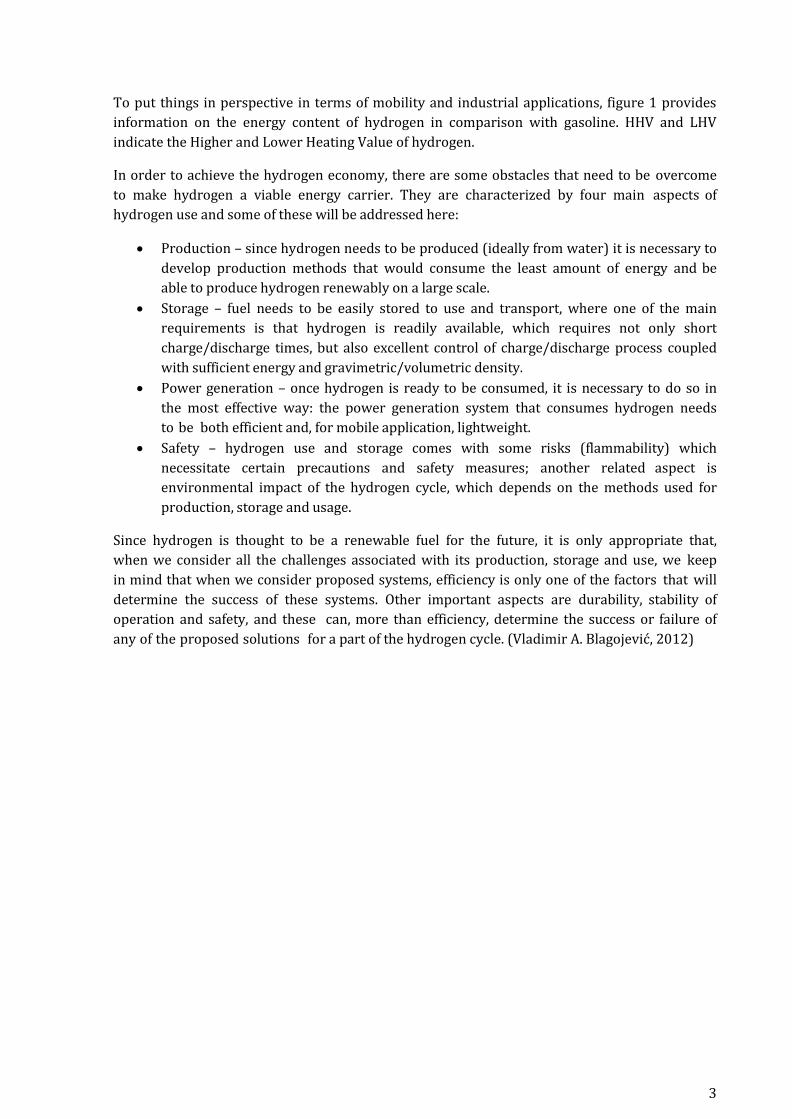
To put things in perspective in terms of mobility and industrial applications, figure 1 provides

information on the energy content of hydrogen in comparison with gasoline. HHV and LHV

indicate the Higher and Lower Heating Value of hydrogen.

In order to achieve the hydrogen economy, there are some obstacles that need to be overcome

to make hydrogen a viable energy carrier. They are characterized by four main aspects of

hydrogen use and some of these will be addressed here:

Production – since hydrogen needs to be produced (ideally from water) it is necessary to

develop production methods that would consume the least amount of energy and be

able to produce hydrogen renewably on a large scale.

Storage – fuel needs to be easily stored to use and transport, where one of the main

requirements is that hydrogen is readily available, which requires not only short

charge/discharge times, but also excellent control of charge/discharge process coupled

with sufficient energy and gravimetric/volumetric density.

Power generation – once hydrogen is ready to be consumed, it is necessary to do so in

the most effective way: the power generation system that consumes hydrogen needs

to be both efficient and, for mobile application, lightweight.

Safety – hydrogen use and storage comes with some risks (flammability) which

necessitate certain precautions and safety measures; another related aspect is

environmental impact of the hydrogen cycle, which depends on the methods used for

production, storage and usage.

Since hydrogen is thought to be a renewable fuel for the future, it is only appropriate that,

when we consider all the challenges associated with its production, storage and use, we keep

in mind that when we consider proposed systems, efficiency is only one of the factors that will

determine the success of these systems. Other important aspects are durability, stability of

operation and safety, and these can, more than efficiency, determine the success or failure of

any of the proposed solutions for a part of the hydrogen cycle. (Vladimir A. Blagojević, 2012)

4

1.1 HYDROGEN PRODUCTION AND APPLICATION

Figure 2: Share of Hydrogen Production (Smolinka, 2014)

There are several potential sources of hydrogen on our planet, although these are

exclusively hydrogen compounds, necessitating extraction of hydrogen at energy cost. The

most abundant is water; hydrogen can also be obtained from hydrocarbons, either fossil fuels

or biomass. Figure 2 gives an overview of share of hydrogen production; it can be seen that

majority of current production is by reforming of hydrocarbons while electrolysis contributes

less than 5 %.

While production from water is clean (given the electricity used is produced by

emission free methods) and renewable (with no CO2 emissions) production from fossil fuels

generates similar or even higher levels of CO2 emissions as burning of coal and gasoline.

Hydrogen production from biomass is carbon neutral, since plants and organisms used during

the process sequester approximately the same amount of CO2 during their growth as it is

emitted during the process of extraction of hydrogen from them. However, their negative

environmental impact is considerable due to the fact that they require large land surfaces to

grow. Since we discuss hydrogen production from electrolysis at length later we review other

methods briefly.

Fossil Fuels

Fossil fuels are the dominant source of industrial hydrogen today. Hydrogen can be

produced from natural gas with efficiency of around 80% and from other hydrocarbon sources

with a varying degree of efficiency. The most widely used method of hydrogen production today

is steam reforming of methane or natural gas. At high temperatures (1000-1300K), water vapor

reacts with methane to yield syngas (mixture of hydrogen and carbon monoxide), which can be

used to produce more hydrogen through reaction of water and carbon monoxide (also known as

water gas shift reaction, performed around 400K). The drawback of this process is that it

produces CO2 waste (Lee, et al., 2001).

48%

30%

18%

4%

Share of Hydrogen Production

Natural Gas

Petroleum

Coal

Electrolysis

5

Other methods of hydrogen production from fossil fuels are partial oxidation of hydrocarbons,

which includes partial combustion of fuel-air mixture at high temperatures or in a presence of a

catalyst, plasma reforming (Kvaerner process), which produces hydrogen and carbon black from

hydrocarbons (no CO2 waste), and coal gasification, where coal is converted to syngas and

methane.

Thermolysis

Water thermolysis is thermal dissociation of water, which occurs spontaneously around

2800K. Although this temperature is too high for practical applications, significant effort has

been invested into research of catalysts to reduce water thermolysis temperature and make it an

industrially viable process. The goal is to use water thermolysis either in solar concentrators or

in nuclear power plants to produce hydrogen directly using thermal energy. Solar concentrators

can produce very high temperatures (over 1800K) by concentrating sunlight using a system of

mirrors. Next generation nuclear power plants will be operating at lower temperatures (1000-

1300K), but it is hoped that new catalysts will make it possible to use them for direct hydrogen

generation using water thermolysis.

Photocatalysis

Photocatalytic water splitting is a process of directly producing hydrogen using solar

energy. It relies on use of photocatalyst to capture the solar energy and use for water

dissociation (Ni, et al., 2007). There are two principal types of catalysts: photoelectrochemical

and photobiological.

Bio hydrogen production

Biological H2 production represents an effort to harness biological processes to

generate hydrogen on the industrial scale. Although they have found no industrial application,

there are a number of processes for conversion of biomass and waste streams into bio

hydrogen. Some of them are the same as the ones described above for fossil fuels, except they

use biomass in place of fossil fuel (biomass gasification, steam reforming), while others use

biological conversion of solar energy (Tao Y., 2007). Biological conversion is process where

biological organisms (usually plants) convert sunlight into hydrogen through their metabolic

processes (Melis, 2002)

In spite of these many methods of hydrogen production, to this date, reforming and electrolysis

remain commercially significant technologies.

6

1.2 ELECTROLYSIS

Electrolysis is an electrochemical process in which electrical energy is the driving force

of chemical reactions. Substances are decomposed, by passing a current through them. The first

observation of this phenomenon was recorded in 1789. Nicholson and Carlisle were the first

who developed this technique back in 1800 and by the beginning of the 20th century there were

already 400 industrial water electrolysis units in use.

The principle of water electrolysis is to pass a direct current between two electrodes

immersed in an electrolyte. Hydrogen is formed at the cathode and oxygen at the anode (positive

terminal). The production of hydrogen is directly proportional to the current passing through

the electrodes. More commonly, Michael Faraday’s laws of electrolysis state that:

The mass of a substance altered at an electrode during electrolysis is directly

proportional to the quantity of electricity Q transferred.

For a given quantity of electric charge Q, the mass of an elemental material altered at an

electrode is directly proportional to the element’s equivalent weight. The equivalent

weight of a substance is equal to its molar mass divided by the change in oxidation

state it undergoes upon electrolysis.

The overall chemical reaction of water electrolysis with required thermodynamic energy values

can be written as

Implementation of a diaphragm or separator is required to avoid recombination of the

hydrogen and oxygen to preserve efficiency and safety. The electrodes, the separator, and the

electrolyte form the electrolytic cell. The electrodes should be resistant to corrosion, have a

good electric conductivity, exhibit good catalytic properties and show a suitable structural

integrity. Furthermore, the electrodes should not react with the electrolyte (Ursúa A, 2012).

Water electrolyzers and fuel cells use similar technology, and the process in fuel cells is the

reverse; hydrogen is converted into electricity and heat. In general, water electrolyzers are

more efficient than fuel cells (Decourt B, 2014)

H2O (l) + 237.2

kJ

mol+ 48.6

kJ

mol = H2 +

1

2O2

(1)

(Electricity) (Heat)

7

1.3 THERMODYNAMICS

In water electrolysis, electrical and thermal energy are converted into chemical

energy, which is partially stored in hydrogen. The energy required for the reaction described in

equation to take place is the enthalpy of formation of water ∆H. Only the free energy of this

reaction, called Gibbs free energy change ∆G, has to be supplied to the electrodes in the form

of electrical energy (McAuli f fe , 1980)The remainder is thermal energy, which is the

product of process temperature T and entropy change ΔS. Enthalpy change can be expressed as

(Faulkner, 1980)

∆𝐻 = ∆𝐺 + 𝑇∆𝑆 = 𝑧𝐹[𝑇(𝜕𝑈𝑟𝑒𝑣/𝜕𝑇)𝑝 − 𝑈𝑟𝑒𝑣] (2) , where z (for hydrogen, z = 2) is the number of moles of electrons transferred in the reaction, F

the Faraday constant (96485.3365 C/mol), Urev the reversible voltage, and p the prevailing

pressure (bar). The reversible cell voltage Urev is the lowest required voltage for the electrolysis

to occur and is also known as the equilibrium cell voltage, or the electro-motive force. The

electrical work done by an electrolytic cell is equal to the free energy change occurring (at

constant temperature and pressure and positive electromotive force).

∆𝐺 = −𝑧𝐹𝑈𝑟𝑒𝑣 (3)

Without thermal energy—heat generation or absorption—the minimum voltage required for

water decomposition is the thermoneutral voltage Utn. At the standard ambient temperature and

pressure (T = 298.15 K, p = 1 bar), the calculated reversible and thermoneutral cell voltages are

Urev = 1.23 V and Utn = 1.48 V (ΔG = 237.21 kJ/mol, ΔS = 0.16 kJ/mol∙K, ΔH = 285.84 kJ/mol). The

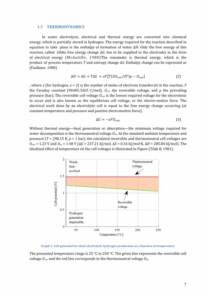
idealized effect of temperature on the cell voltages is illustrated in Figure (Tilak B, 1981).

Graph 1: Cell potential for ideal electrolytic hydrogen production as a function of temperature

The presented temperature range is 25 °C to 250 °C. The green line represents the reversible cell

voltage Urev and the red line corresponds to the thermoneutral voltage Utn

8

As the electrolyte temperature increases, the ideal voltage required to pull water molecules

apart decreases. If the cell potential is under the reversible voltage, hydrogen generation is

impossible. The thermoneutral voltage is the actual minimum voltage that has to be applied to

the electrolytic cell; below this voltage the electrolysis is endothermic, above it is exothermic

and waste heat is produced. If the reaction would take place in the orange-shaded area, the

efficiency would be 100 %, and water splitting would take place by absorbing heat from the

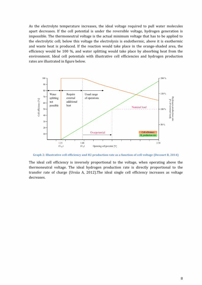
environment. Ideal cell potentials with illustrative cell efficiencies and hydrogen production

rates are illustrated in figure below.

Graph 2: Illustrative cell efficiency and H2 production rate as a function of cell voltage (Decourt B, 2014)

The ideal cell efficiency is inversely proportional to the voltage, when operating above the

thermoneutral voltage. The ideal hydrogen production rate is directly proportional to the

transfer rate of charge (Ursúa A, 2012).The ideal single cell efficiency increases as voltage

decreases.

9

2 OVERVIEW OF WATER ELECTROLYSIS TECHNOLOGIES

There are two basic cell configurations for electrolysis modules: the unipolar and the

bipolar. These configurations are illustrated below in figure 3 and figure 4.

Figure 3: Monopolar cell configuration where electrolysis cells are connected in parallel to form larger modules

UM is the voltage of the electrolysis module and IM is the current of the module.

In monopolar configuration (tank-type), the total cell voltage is equal to the voltage between

individual pairs of electrodes. Module current IM is a sum of cell currents. Each electrode has a

single polarity, hence the name monopolar.

Figure 4: Bipolar cell configuration where electrolytic cells are connected in series

In bipolar configuration (filter-press-type), only the two end electrodes are connected to the DC

power supply. The module voltage UM is a sum of cell voltages in the module. Bi-polar cells are

characterized by their relatively low unit cell voltages, which is due to the shorter current paths

in the electrodes and possibility to achieve narrow inter electrode gaps (Tilak B, 1981).

10

Many manufacturers have developed their electrolyzers from bipolar electrolysis modules since

they are considered more suitable than monopolar ones for hydrogen production due to their

significantly lower ohmic losses (Lehner M, 2014). Additionally to previously present basic

configurations, electrolyzers can also assemble series, parallel, and mixed connections of

modules to achieve the desired production rate. An actual electrolytic hydrogen production

plant requires also additional equipment for gas cooling, purification, compression, and storage.

Production plants also require power supplies, appropriate power conditioning, and safety

control systems (Ursúa A, 2012).

2.1 ALKALINE WATER ELECTROLYZERS

Alkaline electrolysis is widely recognized as a mature technology and the most

developed water electrolysis technology—William Nicholson and Anthony Carlisle were the first

decompose water into hydrogen and oxygen by electrolysis already in 1800 (Gandia, 2013).

Alkaline water electrolyzers account for the majority of the installed water electrolysis capacity

worldwide. Commercial alkaline electrolysis system sizes range from 1.8 to 5300 kW. Hydrogen

production rate (fH2) for commercial systems is 0.25–760 Nm3/hr (Bertuccioli L, 2014) Currently

alkaline electrolyzers are the most suitable option for large-scale hydrogen production, although

they’re rapidly being replaced by PEM ones. The operating principle of an alkaline electrolysis

cell is described in figure below.

Figure 5: The operating principle of an alkaline electrolysis cell

Applied DC voltage decomposes water molecules and the diaphragm passes hydroxide ions from

the cathode to the anode. Hydrogen is formed at the cathode and oxygen at the anode.

In an alkaline electrolysis cell, which is typically housed in a steel compartment, the two

electrodes are separated by a gas-tight diaphragm submerged in a liquid electrolyte. To improve

the ionic conductivity of the electrolyte, the electrolyte is usually a 20–40 wt% aqueous solution

of potassium hydroxide (KOH), which is preferred over sodium hydroxide (NaOH) due to its

higher conductivity. Neglecting physical losses, the liquid electrolyte is not consumed. Since

water is consumed in water electrolysis, it has to be supplied continuously (Lehner M, 2014).

Product gases leaving the cell are separated from the remaining electrolyte which is pumped

back into the cell. The electrolyte distribution system and gas separation from the liquid

electrolyte is illustrated in figure 5.

11

Figure 6: Overview of a typical alkaline electrolysis plant viewed from the hydrogen side (cathode)

Product (wet) gases from the electrolyzer stacks rise to the gas separator tanks where they are

separated from the remaining electrolyte. Oxygen gas is treated in its own gas separator tank.

Water is continuously added into the system to maintain the desired electrolyte concentration

(Tilak B, 1981).

As an adverse effect to increasing the conductivity of the electrolyte, potassium hydroxide gives

the electrolyte solution a corrosive nature. The electrodes are usually made of nickel or nickel

plated steel (Lehner M, 2014). The diaphragms have previously been made of asbestos

(McAuliffe, 1980) but nowadays they are mainly based on sulphonated polymers, polyphenylene

sulphides, polybenzimides, and composite materials. The diaphragm must keep the product

gasses apart to maintain efficiency and safety. The diaphragm also has to be permeable to the

hydroxide ions and water molecules. The electrical resistance of the diaphragm is frequently

three to five times that of the electrolyte (Otero J, 2014)

Chemical reactions taking place in alkaline electrolysis at the cathode and the anode,

respectively, are as follows

2H2O + 2e− = H2(g) + 2OH−

(4)

2OH−(aq) = 12⁄ O2(g) + H2O(l) + 2e−

(5)

Hydrogen is formed at the cathode where water is reduced; Hydroxide anions circulate across

the diaphragm to the anode. The formed hydrogen can reach a purity level between 99.5–

99.9998 % (Bertuccioli L, 2014). Water fed to an alkaline electrolyzer has to be pure with an

electrical conductivity below 5 μS/cm. Characteristics of alkaline electrolyzers are listed in table

1 below,

12

Parameters Values

Current density 0.2–0.4 A/cm2

Cell area < 4 m2

Hydrogen output pressure 0.05–30 bar

Operating temperature 60–80 °C

Minimum load 20–40 % 5 % (state of the art)

Overload < 150 % (nominal load)

Ramp-up from minimum load to full load

0.13–10 % (full load)/second

Start-up time from cold to minimum load

20 min – several hours

H2 purity 99.5–99.9998 %

System efficiency (HHV) 68–77 %

Indicative system cost 1.0–1.2 €/W

System size range 0.25–760 Nm3/h 1.8–5300 kW

Lifetime stack 60 000–90 000 hrs

Table 1: Alkaline electrolyzer characteristics (Carmo M, 2013)

The minimum partial load of alkaline electrolyzers is limited by the diaphragm, which cannot

completely prevent the product gasses from cross-diffusing through it. The diffusion of oxygen

into the cathode side reduces the electrolyzer’s efficiency by forcing the oxygen to catalyze back

to water with the hydrogen. Hydrogen diffusion to the anode side also occurs and must be

avoided to preserve efficiency and safety. The cross-diffusion of product gasses is particularly

severe at low loads and can result in flammable gas mixtures, hence the typically high minimum

partial load of alkaline electrolyzers. The current density of alkaline electrolyzers is limited by

the ohmic losses across the liquid electrolyte and the diaphragm. The liquid electrolyte also

results in a bulky stack design configuration (Carmo M, 2013). Additionally, the liquid electrolyte

renders alkaline electrolyzers unable to quickly react to changes in input power due to the delay

caused by the inertia of the liquid.

(Ulleberg, 2003) listed three basic improvements that can be implemented in the design of

advanced alkaline electrolyzers; 1) new cell configurations to reduce the surface-specific cell

resistance (e.g. zero-gap cells and low-resistance diaphragms), 2) higher process temperatures

up to 160 °C, and 3) new electro catalysts to reduce the electrode overpotentials (cobalt oxide at

the anode and Raney-nickel coatings at the cathode).

13

2.2 PROTON EXCHANGE MEMBRANE (PEM) ELECTROLYZERS

Figure 7: Operating principle of proton exchange membrane electrolyzers (Siemens AG)

The electrolyte in PEM electrolyzer is a gas-tight thin polymeric membrane, which has a

proton H+ conducting ability. H+ protons pass through the polymer electrolyte membrane and at

the cathode combine with electrons to form hydrogen.

In PEM electrolyzers, thin (50–250 μm) proton conducting membrane is used as a solid polymer

electrolyte rather than liquid electrolytes typically used in alkaline water electrolyzers (Lehner

M, 2014). The polymer electrolyte membranes have a strongly acid character and are

mechanically strong. Common theme is to use sulphonated fluoropolymers, usually

fluoroethylene. The most established one of these is Nafion™. The basic polymer, polyethylene, is

modified by substituting fluorine for the hydrogen and this chemical compound is further

sulfonated by adding a side chain ending with sulphonic acid HSO3. Thus, a polymeric electrolyte

is formed. The added HSO3 group is ionically bonded and due to the ionic bonding there’s a

strong mutual attraction between H+ and SO3- from each molecule. An essential property of

sulphonic acid is that it attracts water, and the conductivity of the polymer electrolyte

membrane is dependent on hydration—decreasing water content decreases conductivity.

Mixing of water and the ionic bonding of the sulphonic acid group enable the H+ protons to

move through the molecular structure.

General Electric developed the first water electrolyzer based on the polymer electrolyte

membrane by 1966 and began to commercialize the concept in 1978 (Ursúa A, 2012). Today,

PEM electrolysis is regarded as a commercial technology only at small and medium scale

applications (Bertuccioli L, 2014). Still, only a few companies are manufacturing PEM water

electrolyzers due to their higher investment cost and typically shorter lifetime compared to

alkaline water electrolyzers. The high investment cost is due to the material requirements set by

the corrosive low pH conditions of the polymer electrolyte membrane. The corrosion resistance

requirement applies also to current collectors and separator plates. This creates a demand for

14

scarce, expensive materials and components such as noble catalysts (platinum-group metals

(PGM) e.g. platinum, iridium, and ruthenium), titanium-based current collectors, and separator

plates (Carmo et al. 2013). Chemical reactions taking place in PEM electrolysis at anode and

cathode, respectively, are as follows (Ursúa et al. 2012a)

𝐻2𝑂(𝑙) = 12⁄ 𝑂2(𝑔) + 2𝐻+ + 2𝑒−

(6)

2𝐻+(𝑎𝑞. ) + 2𝑒− = 𝐻2(𝑔)

(7)

Deionized water is fed to the anode side where the oxygen evolution reaction occurs. Water

travels in separator plates and diffuses through the current collectors. Then the water reaches

the anode catalyst layer (IrO2) and decomposes. Formed oxygen has to travel against the water

flow back to the separator plates and out of the cell. Electron path from the catalytic layer of the

anode is through the current collectors and separator plates to the cathode side. Protons leave

the anode catalytic layer through an ionomer (typically Nafion ionomer) and crossing through

the membrane to the cathode side of the cell. On the cathode side, the protons combine with the

electrons to form hydrogen gas at the cathode catalyst layer (Pt). Formed hydrogen gas then has

to flow through the cathode side’s current collector and separator plate to leave the cell (Carmo

M, 2013). Example of a PEM electrolyzer cell stack is illustrated below.

Figure 8: High-pressure PEM electrolyzer cell stack comprising 12 series-connected cells with a 160 cm2 active area per cell. The cathode pressure in normal operation can be 35 bar while the anode pressure stays

at 3.5 bar (Marangio F, 2009)

Due to a low gaseous permeability provided by the solid polymer membrane, the product

hydrogen purity is higher than in alkaline electrolysis, typically above 99.99 % without the need

of auxiliary equipment. The electrical conductivity of water fed to a PEM electrolyzer has to be

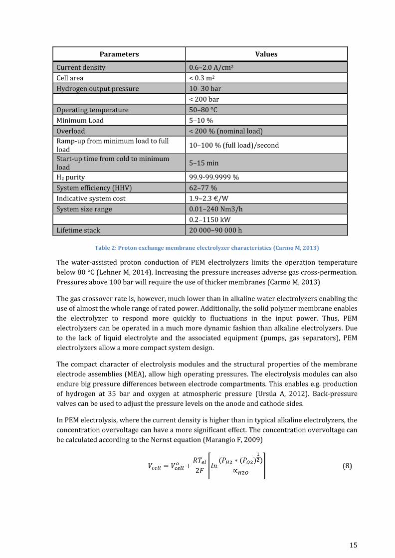
below 1 μS/cm Characteristics of PEM water electrolyzers are listed in table below.

15

Parameters Values

Current density 0.6–2.0 A/cm2

Cell area < 0.3 m2

Hydrogen output pressure 10–30 bar

< 200 bar

Operating temperature 50–80 °C

Minimum Load 5–10 %

Overload < 200 % (nominal load)

Ramp-up from minimum load to full load

10–100 % (full load)/second

Start-up time from cold to minimum load

5–15 min

H2 purity 99.9-99.9999 %

System efficiency (HHV) 62–77 %

Indicative system cost 1.9–2.3 €/W

System size range 0.01–240 Nm3/h

0.2–1150 kW

Lifetime stack 20 000–90 000 h

Table 2: Proton exchange membrane electrolyzer characteristics (Carmo M, 2013)

The water-assisted proton conduction of PEM electrolyzers limits the operation temperature

below 80 °C (Lehner M, 2014). Increasing the pressure increases adverse gas cross-permeation.

Pressures above 100 bar will require the use of thicker membranes (Carmo M, 2013)

The gas crossover rate is, however, much lower than in alkaline water electrolyzers enabling the

use of almost the whole range of rated power. Additionally, the solid polymer membrane enables

the electrolyzer to respond more quickly to fluctuations in the input power. Thus, PEM

electrolyzers can be operated in a much more dynamic fashion than alkaline electrolyzers. Due

to the lack of liquid electrolyte and the associated equipment (pumps, gas separators), PEM

electrolyzers allow a more compact system design.

The compact character of electrolysis modules and the structural properties of the membrane

electrode assemblies (MEA), allow high operating pressures. The electrolysis modules can also

endure big pressure differences between electrode compartments. This enables e.g. production

of hydrogen at 35 bar and oxygen at atmospheric pressure (Ursúa A, 2012). Back-pressure

valves can be used to adjust the pressure levels on the anode and cathode sides.

In PEM electrolysis, where the current density is higher than in typical alkaline electrolyzers, the

concentration overvoltage can have a more significant effect. The concentration overvoltage can

be calculated according to the Nernst equation (Marangio F, 2009)

𝑉𝑐𝑒𝑙𝑙 = 𝑉𝑐𝑒𝑙𝑙𝑜 +

𝑅𝑇𝑒𝑙

2𝐹[𝑙𝑛

(𝑃𝐻2 ∗ (𝑃𝑂2)12)

∝𝐻2𝑂] (8)

16

Where Pi is the partial pressure of the species i, R is the universal gas constant, Tel is the average

electrolyzer cell temperature, F is the faraday’s constant and 𝑉𝑐𝑒𝑙𝑙𝑜 is the reversible cell voltage at

standard temperature and pressure.

The concentration over-voltage is negligible when the operating current density is below 1

A/cm2 (Nieminen J, 2010). However, (García-Valverde R, 2012) asserted that concentration

overpotential would be significant only at very high current densities and would therefore be

hardly seen in commercial PEM water electrolyzers. Simulated cell voltage for a proton exchange

membrane electrolyzer is illustrated in graph below.

Graph 3: Simulated cell voltage in PEM water electrolysis at T = 75 °C and p = 30 bar. Limiting current density was given a constant value of 2 A/cm2 (Nieminen J, 2010)

Commercial PEM electrolyzers typically operate at current densities of 0.6–2.0 A/cm2 (Carmo M,

2013). The concentration overvoltage is more significant in PEM water electrolysis, but can be

ignored in alkaline electrolysis where the current density is typically below 0.5 A/cm2.

Alkaline electrolysis PEM electrolysis SOEC electrolysis

Advantages

Well established technology

High current densities Efficiency up 100%

thermoneutral

Non noble catalysts High voltage efficiency Efficiency > 100% w/hot steam

Long-term stability Good partial load range Non noble catalysts

Relative low cost Rapid system response High pressure operation

Stacks in the MW range Compact system design

Cost effective High gas purity

Dynamic operation

Disadvantages

Low Current Densities High cost of components Laboratory stage

Lower degree of purity Acidic corrosive

environment Bulky system design

Low partial load range Possibly low durability Durability (brittle ceramics)

Low operational pressures Commercialization

Table 3: Comparison of Electrolyzer technologies (Carmo M, 2013)

17

To summarize, alkaline and PEM are the two main water electrolysis technologies, which are

commercially available. Alkaline water electrolysis is the more matured and widespread of the

two technologies. The high cost of components and scale-up procedures in PEM electrolysis have

limited the number of PEM electrolyzer manufacturers. Furthermore, alkaline electrolyzer cells

typically have longer lifetimes than PEM electrolyzer cells. However, PEM technology has

various advantages over alkaline systems, such as compact system design, lack of liquid

electrolyte, wide partial load range, and high flexibility in modes of operation. Therefore, PEM

electrolysis is an intriguing option when integration into renewable power generating systems is

considered. Additionally, PEM technology has been studied in unitized regenerative fuel cell

(URFC) systems. A URFC is a reversible electrochemical device, which can operate either as an

electrolyzer producing hydrogen and oxygen from water or as a H2/O2 fuel cell producing

electricity and heat.

2.3 SOLID OXIDE ELECTROLYTE ELECTROLYZERS

Solid oxide electrolyte (SOE) electrolysis is the third main water electrolysis technology

besides alkaline and PEM technologies. SOE electrolysis is the least mature of the three main

electrolysis technologies, still being in R&D stage (Lehner M, 2014).

The SOE technology is not new, since pioneering work was done in the late 1960s (Ursúa A,

2012) SOE technology is gaining growing interest due to its potential to increase the efficiency of

water electrolysis by using high operating temperatures, typically 700–1000 °C. Therefore, SOE

is actually steam electrolysis. However, such high temperatures cause severely fast degradation

of the cell components, and thus keep SOE electrolysis in the R&D stage. Understanding of the

detailed mechanisms behind degradation is still not well established. To gain thermal stability of

the materials, research efforts are focusing on SOE systems operated at 500–700 °C. For the

same reason, current densities are kept in the range of 0.3–0.6 A/cm2. The corresponding cell

voltages are around 1.2–1.3 V, which result in low electrical energy consumptions. Taking the

energy demands for electricity and heat into account, the system efficiencies are typically over

90 % (Lehner M, 2014) SOE electrolyzers can also be operated in reverse mode and used in

URFC systems. SOE electrolyzer cells are actually often modified from solid oxide fuel cells

(SOFC).

Chemical reactions taking place in SOE electrolysis at cathode and anode, respectively, are as

follows (Ursúa A, 2012)

H2O (g) + 2e− = H2(g) + O2−

O2− = 12⁄ O2(g) + 2e−

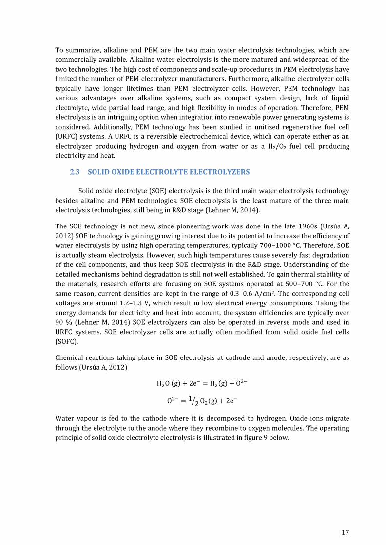
Water vapour is fed to the cathode where it is decomposed to hydrogen. Oxide ions migrate

through the electrolyte to the anode where they recombine to oxygen molecules. The operating

principle of solid oxide electrolyte electrolysis is illustrated in figure 9 below.

18

Figure 9: Operating principle of solid oxide electrolyte electrolyzers

Core components are typically made of ceramic materials. Most widely used electrolyte material

in high-temperature SOE electrolysis is yttria-stabilized zirconia (YSZ) (Lehner M, 2014). In

studies regarding electrolyte materials for SOFC, scandia-stabilized zirconia is known to exhibit

highest conductivity (Sarat S, 2006). Anode materials are typically composite electrodes of YSZ

with perovskite type mixed oxides, e.g. lanthanum strontium cobalt ferrite used in SOFCs.

Cathode materials are commonly a mixture (cermet) of Ni and ion conducting particles similar to

the electrolyte material (Lehner M, 2014). PGM catalysts are not needed due to high operating

temperatures, but precious metal is used for thin electrical contact layers.

19

3 TEST BENCH

Figure 10: Test Bench

3.1 COMPONENT SUMMARY OF THE TEST BENCH

The following tables detail every component of in the test bench used to perform the experiments.

Anode side

Component Code Function

Back pressure regulator

BPR-101 Pressurize in the range 0,6-3 bar g


BPR-102 Pressurize in the range 3-15 bar g

Ball valve BV-101 Manual discharge of GLS-101

Dosing pump DP-101 Pump water into the Electrolyzer (Anode side)

Electric heating EH-101 Heat up water up to 80°C

Electric heating EH-102 Heat up oxygen up to 40°C

Gas dryer GD-101 Condense the humidity from the oxygen stream Gas/liquid separator

GLS-101 Contain water and separate gaseous oxygen from liquid water

Ion exchanger IE-101 Lower the electric conductivity of the liquid water that enters the Electrolyzer (Anode side)

Relief valve RV-101 Release the pressure in GLS-101, should it exceed 15 bar g

Solenoid valve V-101 Disconnect hydraulically GLS-101 from DP-101

Solenoid valve V-102 Prevent oxygen from flowing into BPR-101 and BPR-102

Solenoid valve V-103 Prevent oxygen from flowing into BPR-102 (high pressure side)

Solenoid valve V-104 Prevent oxygen from flowing into BPR-102 (low pressure side)

Solenoid valve V-105 Automatic discharge of GLS-101

Table 4: Process components of the anode side of the test bench

20

Cathode side



BPR-201 Pressurize in the range 0-3 bag


BPR-202 Pressurize in the range 3-15 bag

Ball valve BV-201 Manual discharge of GLS-201

Dosing pump DP-201 Pump water into the Electrolyzer (Cathode side) Electric heating EH-201 Heat up water up to 80°C

Electric heating EH-202 Heat up oxygen up to 40°C

Gas dryer GD-201 Condense the humidity from the hydrogen stream

Gas/liquid separator

GLS-201 Contain water and separate gaseous hydrogen from liquid water

Ion exchanger IE-201 Lower the electric conductivity of the liquid water that enters the Electrolyzer (Cathode side)

Relief valve RV-201 Release the pressure in GLS-201, should it exceed 15 bar g

Solenoid valve V-201 Disconnect hydraulically GLS-201 from DP-201

Solenoid valve V-202 Prevent hydrogen from flowing into BPR-201 and BPR-202

Solenoid valve V-203 Prevent hydrogen from flowing into BPR-202 (high pressure side)

Solenoid valve V-204 Prevent hydrogen from flowing into BPR-202 (low pressure side)

Solenoid valve V-205 Automatic discharge of GLS-201

Table 5: Process components of the cathode side of the test bench

Water supply


Check valve CV-301 Prevent high pressure water from entering the water supply system

Solenoid valve V-301 Automatically open or close water supply into the system

Solenoid valve V-302 Automatically open or close water supply into GLS-101

Solenoid valve V-303 Automatically open or close water supply into GLS-201

Solenoid valve V-304 Automatically open or close nitrogen supply into GLS-201

Solenoid valve V-305 Automatically open or close hydrogen supply into GLS-201

Table 6: Process components of the water supply of the test bench.

Power supply


Controllable power supply PS-401 Provide DC current to the Electrolyzer

Table 7: Process components of the power supply of the test bench

This test bench used for all the experiments was built by my supervisor Julio César

García Navarro as a part of his ongoing doctoral thesis. The flexibility of the testing bench allows

testing on a wide range of parameters. One of the unique features of the test bench is the ability

to vary the water flow on both the anode and cathode side using two different pumps. The

pressure and temperature also can be independently controlled on either cathode or anode

sides. This has allowed testing of individual flow rate & pressure on performance and helped in

identifying the most degrading mechanism of the PEM electrolyzer. Due to the small size and

proximity of the system, having a temperature gradient across anode and cathode plates is not

feasible.

21

3.2 EXPLODED VIEW OF THE ELECTROLYZER

Figure 11: Exploded view of the electrolyzer cell

ID Component Name

a Cathode End Plate

b Cathode side gasket

c Titanium Current Collector – Cathode

d Membrane Electrode Assembly Nafion 115

e Titanium Current Collector – Anode

f Anode side gasket

g Flow field

h Anode End Plate

The Nafion 115 MEAs used in the experiments were made by Baltic Fuel Cells GmBH. They were

catalyst coated membranes with cathode loading of 1.2 – 1.4 mg Pt/cm2 and anode loading of 2

mg IR black/cm2. The Titanium current collectors were used due to their high corrosion

resilience to the Oxygen Evolution Reaction (OER). The single cell electrolyzer was composed of

one current collector plate and two flow field plates with an MEA between them, sealed with

gaskets. Figure 11 shows the assembly of the electrolyzer. The end plate was used primarily for

electrical connection and structural strength. The water supply was connected to the end plates.

Heating pads were situated in the end plates to heat up the water inside the electrolyzer.

The water was guided through the end plate to the flow fields where it is consumed and then

guided back to the end plate and out of the electrolyzer. Temperature probes were connected in

the end plates to measure the temperature of the electrolyzer. The current collector plates were

22

isolated from the endplates. The cathode end plate was coated with gold and has as integrated

flow field.

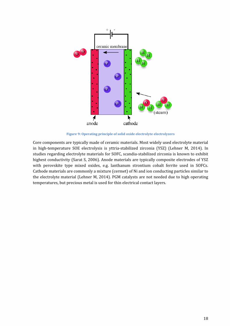
The MEA is the anode electrocatalyst, membrane and cathode catalyst combined. The anode

electro-catalyst plays the most significant role in the electrolyzer while the cathode electro-

catalyst activity is often neglected. The membranes often used are Nafion 115, 117 and 1110.

The MEA is sealed with a gasket on each side. The figure 12 gives a summary of materials used

for various components of electrolyzer.

Figure 12: Component material summary of PEM electrolyzer

Bipolar Plate

Porous Current Collector

(GDL)

Electrocatalytic Layers

Polymer Electrolyte

Membrane

Electrocatalytic Layers

Porous Current Collector

(GDL)

Bipolar Plate

Graphite, Stainless steel, Titanium, Boron-doped diamond (BDD) coated

titanium and mixed metal oxide (MMO) coated titanium

Ir black, Pt

,Ru[36]

Pt black, Pt

Graphite, Stainless steel, Titanium, Boron-doped diamond (BDD) coated titanium and mixed metal oxide (MMO) coated titanium

Sintered Porous Titanium (SPT), Graphite, carbon

based material

Perfluorosulfonic acid polymer

(Nafion 115) (Nafion®,

Fumapem®, Flemion®,

Aciplex®

Sintered Porous Titanium (SPT), Graphite, carbon

based material

ANODE

CATHODE

MATERIAL MATERIAL COMPONENT

23

4 LOSSES IN A PEM ELECTROLYZER

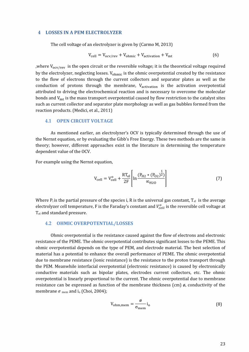
The cell voltage of an electrolyzer is given by (Carmo M, 2013)

Vcell = Vocv/rev + Vohmic + Vactivation + Vmt (6)

,where Vocv/rev is the open circuit or the reversible voltage; it is the theoretical voltage required

by the electrolyzer, neglecting losses. Vohmic is the ohmic overpotential created by the resistance

to the flow of electrons through the current collectors and separator plates as well as the

conduction of protons through the membrane, Vactivation is the activation overpotential

attributed to driving the electrochemical reaction and is necessary to overcome the molecular

bonds and Vmt is the mass transport overpotential caused by flow restriction to the catalyst sites

such as current collector and separator plate morphology as well as gas bubbles formed from the

reaction products. (Medici, et al., 2011)

4.1 OPEN CIRCUIT VOLTAGE

As mentioned earlier, an electrolyzer’s OCV is typically determined through the use of

the Nernst equation, or by evaluating the Gibb’s Free Energy. These two methods are the same in

theory; however, different approaches exist in the literature in determining the temperature

dependent value of the OCV.

For example using the Nernst equation,

Vcell = Vcello +

RTel

2F[ln

(PH2 ∗ (PO2)12)

∝H2O] (7)

Where Pi is the partial pressure of the species i, R is the universal gas constant, Tel is the average

electrolyzer cell temperature, F is the Faraday’s constant and 𝑉𝑐𝑒𝑙𝑙𝑜 is the reversible cell voltage at

Tel and standard pressure.

4.2 OHMIC OVERPOTENTIAL/LOSSES

Ohmic overpotential is the resistance caused against the flow of electrons and electronic

resistance of the PEME. The ohmic overpotential contributes significant losses to the PEME. This

ohmic overpotential depends on the type of PEM, and electrode material. The best selection of

material has a potential to enhance the overall performance of PEME. The ohmic overpotential

due to membrane resistance (ionic resistance) is the resistance to the proton transport through

the PEM. Meanwhile interfacial overpotential (electronic resistance) is caused by electronically

conductive materials such as bipolar plates, electrodes current collectors, etc. The ohmic

overpotential is linearly proportional to the current. The ohmic overpotential due to membrane

resistance can be expressed as function of the membrane thickness (cm) ø, conductivity of the

membrane 𝜎 mem and io (Choi, 2004);

Vohm,mem =ø

σmemio (8)

24

Where Rion = ø

σmem is the ionic resistance. The local ionic conductivity with water content and

temperature function can be written as

σmem = (0.005139γ − 0.00326)exp [1268 (

1

303−

1

Tel)] (9)

Where, 𝛾 is the degree of membrane humidification.

The interfacial overpotential can be expressed as

Vohm,ele = Releio (10)

The ohmic resistance of the electronic materials as the function of the material resistivity Ψ in

(Ωm), the length of electrons path l, and A the conductor cross-sectional area is given by,

Rele = Ψl/A (11)

As a result the ohmic overpotential can be expressed as,

Vohm = (Rele + Rion)io (12)

Although all these overpotentials are present, the resistance of the proton exchange membrane

contributes the most of the total ohmic resistance.

4.3 ACTIVATION OVERPOTENTIAL/LOSSES

Activation overpotential represents the overpotential to initiate the proton transfer and

the electrochemical kinetic behavior in the PEME. Some portion of the applied voltage is lost as

result of transferring the electrons to or from the electrodes during chemical reactions at the

electrodes. The activation energy required at both the anode and the cathode due to the

activation over-potential can be given by relating the Butler-Volmer expression. The activation

overpotential at anode and cathode can be written for a PEME as (García-Valverde R, 2012)

Vact,a =

RT

αazFln (

ia

io,a) (13)

Vact,c =

RT

αczFln (

ic

io,c) (14)

, where R is the universal gas constant, R = 8.314 J K-1 mol-1, z is the stoichiometric coefficient

refers to the number of electrons transferred in the global half cell (defined by Faraday's law).

The value of the stoichiometric coefficient in water electrolysis is 2. 𝛼𝑎 and 𝛼𝑐 are the charge

transfer coefficients. Their values are 0.5 on the symmetric reactions.

The charge transfer resistance is the resistance of the barrier through which the electrons

pass through from the electrode surface to the adsorbed species or from the species to the

25

electrode. Put differently, this is the loss which electrons need to overcome to cross the

interface. The Vactivation is given by the sum of (13) and (14).

4.4 MASS TRANSPORT OVERPOTENTIAL/LOSSES

There have been intensive studies on the mass transport for fuel cell systems. However,

very few mass transport phenomena are available for PEM electrolyzer (Marangio F, 2009) (Lee,

et al., 2013) (Trinke, et al., 2017). Mass transport can be categorized into two groups, namely

water transport and gases crossover. (Rahim Abdol, et al., 2016) has studied these mass

transport losses in considerable detail.

Though other approaches exist, in the field of electrolysis the mass flow through the porous

current collectors is typically explained as a diffusion phenomenon. Computationally this is

achieved through the application of Fick’s Law, which for diffusion in the x-axis direction is,

J = −Deff (

∂Ci

∂x) (15)

, where J is the diffusion flux, Deff is the effective diffusivity of the transport media, and Ci is the

molar concentration of species i. (Medici, et al., 2010)

To predict the voltage loss due to a surplus of reaction products at the catalyst sites blocking the

reactants the Nernst equation can be combined with Fick’s law to create a diffusion rate that

limits the reaction rate at higher current densities. This approach, referred to as the diffusion

driven approach herein, can be applied for both the cathode and the anode accounting for the

greatly differing diffusion rates of hydrogen and oxygen.

Vtrans,an =

RT

zFln (

cO2,mem

cO2,mem,0) (16)

Vtrans,cat =

RT

zFln (

cH2,mem

cH2,mem,0) (17)

In the calculation of the voltage loss due to mass transport Ci,mem is the concentration of species i

at the membrane-electrode interface and Ci,mem,0 is a working condition taken as a reference. In

the work by (Marangio F, 2009), the diffusion driven approach is derived in a more in-depth

manner.

Alternatively, a multiphase flow through porous media can be described by assuming a specified pore network or deriving a network through intensive image processing (Wargo EA, 2012) and modeling the flow through the individual pores using the Poiseuille equation. This approach, which is referred to as the momentum driven approach, has been used in fuel cell modeling to capture the effects of morphology on the gas diffusion layers

Q =πr4∆P

8μL (18)

26

(Carmo M, 2013) , where Q is the volumetric flow rate through the pore, L is the length of the

pore, 𝜇 is the viscosity of the fluid, and r is the radius of the pore.

Ideally, water flows only at the anode channel. In reality, however, a portion of the water

permeates the MEA into the cathode channel. (Marangio F, 2009) estimated the influence of

temperature and pressure on the diffusion coefficient of hydrogen ions. As expected, the

diffusion coefficient of hydrogen ions in the PEM increased with increasing temperature, and

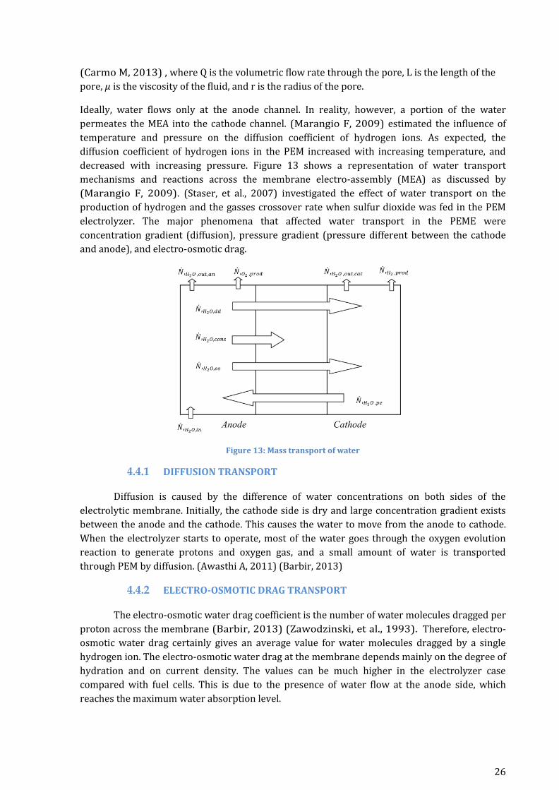
decreased with increasing pressure. Figure 13 shows a representation of water transport

mechanisms and reactions across the membrane electro-assembly (MEA) as discussed by

(Marangio F, 2009). (Staser, et al., 2007) investigated the effect of water transport on the

production of hydrogen and the gasses crossover rate when sulfur dioxide was fed in the PEM

electrolyzer. The major phenomena that affected water transport in the PEME were

concentration gradient (diffusion), pressure gradient (pressure different between the cathode

and anode), and electro-osmotic drag.

Figure 13: Mass transport of water

4.4.1 DIFFUSION TRANSPORT

Diffusion is caused by the difference of water concentrations on both sides of the

electrolytic membrane. Initially, the cathode side is dry and large concentration gradient exists

between the anode and the cathode. This causes the water to move from the anode to cathode.

When the electrolyzer starts to operate, most of the water goes through the oxygen evolution

reaction to generate protons and oxygen gas, and a small amount of water is transported

through PEM by diffusion. (Awasthi A, 2011) (Barbir, 2013)

4.4.2 ELECTRO-OSMOTIC DRAG TRANSPORT

The electro-osmotic water drag coefficient is the number of water molecules dragged per

proton across the membrane (Barbir, 2013) (Zawodzinski, et al., 1993). Therefore, electro-

osmotic water drag certainly gives an average value for water molecules dragged by a single

hydrogen ion. The electro-osmotic water drag at the membrane depends mainly on the degree of

hydration and on current density. The values can be much higher in the electrolyzer case

compared with fuel cells. This is due to the presence of water flow at the anode side, which

reaches the maximum water absorption level.

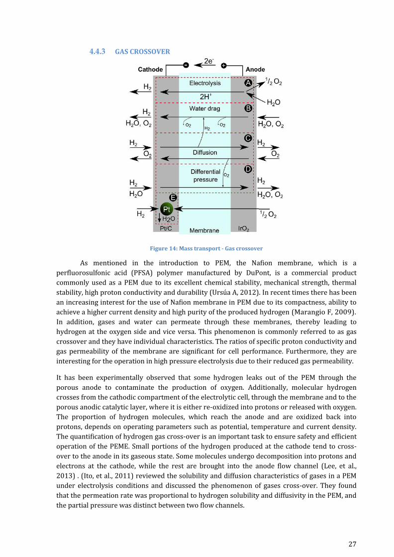
27

4.4.3 GAS CROSSOVER

Figure 14: Mass transport - Gas crossover

As mentioned in the introduction to PEM, the Nafion membrane, which is a

perfluorosulfonic acid (PFSA) polymer manufactured by DuPont, is a commercial product

commonly used as a PEM due to its excellent chemical stability, mechanical strength, thermal

stability, high proton conductivity and durability (Ursúa A, 2012). In recent times there has been

an increasing interest for the use of Nafion membrane in PEM due to its compactness, ability to

achieve a higher current density and high purity of the produced hydrogen (Marangio F, 2009).

In addition, gases and water can permeate through these membranes, thereby leading to

hydrogen at the oxygen side and vice versa. This phenomenon is commonly referred to as gas

crossover and they have individual characteristics. The ratios of specific proton conductivity and

gas permeability of the membrane are significant for cell performance. Furthermore, they are

interesting for the operation in high pressure electrolysis due to their reduced gas permeability.

It has been experimentally observed that some hydrogen leaks out of the PEM through the

porous anode to contaminate the production of oxygen. Additionally, molecular hydrogen

crosses from the cathodic compartment of the electrolytic cell, through the membrane and to the

porous anodic catalytic layer, where it is either re-oxidized into protons or released with oxygen.

The proportion of hydrogen molecules, which reach the anode and are oxidized back into

protons, depends on operating parameters such as potential, temperature and current density.

The quantification of hydrogen gas cross-over is an important task to ensure safety and efficient

operation of the PEME. Small portions of the hydrogen produced at the cathode tend to cross-

over to the anode in its gaseous state. Some molecules undergo decomposition into protons and

electrons at the cathode, while the rest are brought into the anode flow channel (Lee, et al.,

2013) . (Ito, et al., 2011) reviewed the solubility and diffusion characteristics of gases in a PEM

under electrolysis conditions and discussed the phenomenon of gases cross-over. They found

that the permeation rate was proportional to hydrogen solubility and diffusivity in the PEM, and

the partial pressure was distinct between two flow channels.

28

(Schalenbach, et al., 2013) assumed that the entire hydrogen permeation flux density across the

membrane is the sum of the diffusion flux density and the permeation flux density due to

differential pressure. The figure 14 shows the mass transport phenomenon in a single cell of

PEME where: (A) shows the proton flux of the water electrolysis; (B) shows that due to the

proton flux, water and dis- solved oxygen and hydrogen can be electro-osmotically dragged from

the anode to the cathode. During transportation, the gases are diluted into the surrounding

water; (C) shows the diffusion of oxygen and hydrogen; (D) shows the permeation due to

differential pressure; and (E) illustrates the catalytic reaction of hydrogen and oxygen on the

cathodic platinum catalyst.

29

5 ELECTROCHEMICAL IMPEDANCE SPECTROSCOPY

5.1 INTODUCTION TO EIS

Electrochemical Impedance Spectroscopy (EIS) is a powerful technique for the

characterization of electrochemical systems. The premise of EIS is that, with a single

experimental procedure encompassing a sufficiently broad range of frequencies, the influence

of the governing physical and chemical phenomena may be isolated and distinguished at a

given applied potential.

Electrochemical impedance spectroscopy is well known in the electrochemical field as an in-situ

as well as ex-situ method. The introduction of fuel cells in the late 1950’s linked electrochemists

and material scientists. The focus of analyses shifted from the time domain to a frequency

domain, towards a small perturbation signal.

In recent years, EIS has found widespread applications in the field of characterization of

materials. It is routinely used in the characterization of coatings, batteries, fuel cells, and

corrosion phenomena. It has also been used extensively as a tool for investigating mechanisms

in electro–deposition, electro dissolution, passivity, and corrosion studies.

Techniques such as current interruption, cyclic voltammetry, potential sweeping and EIS have

been used to investigate different aspects of the electrolyzer. The polarization curve

characteristics are useful to identify important electrochemical parameters such as exchange

current densities, Tafel slopes and diffusion coefficients. Polarization curves provide only

important data of the performance of the electrolyzer. Unfortunately polarization curves provide

no information about the membrane-electrode interface mechanisms and the individual

contribution of each process occurring at the electrode level. Current interruption on the other

hand is a method used only to measure the ohmic and activation resistance of a membrane. EIS is a

technique frequently applied and recently it is known as a primary tool in fuel cell research.

One of the most attractive aspects of impedance spectroscopy as a tool for investigating the

electrical and electrochemical properties of materials and systems is the direct connection

that often exists between the behavior of a real system and that of an idealized circuit model

consisting of electrical components. The investigator typically compares or fits the impedance

data to an equivalent circuit model, which is a representation of the physical processes taking

place in the system under investigation.

5.2 PRINCIPLES OF EIS MEASUREMENT

A small perturbation of AC current is applied while the electrolyzer is operating at

steady state conditions. There are three different types of electrical perturbations which are

used in the electrochemical field:

First, in the transient measurements a step function (V (t) = V0 for t > 0, V (t) = 0, for t <0 is

applied at t = 0 to the system. The corresponding time- varying current i(t) is measured. The

relationship V0/I (t) is called the time varying resistance. The advantage of this method is that

it is experimentally easily accomplished. The disadvantage is that the results must be

transformed with the Fourier or Laplace-transform and the signal-to-noise ratio varies at

different frequencies. This method is easy to formulate but not often used in EIS.

30

The second method is to compose the stimuli voltage v(t) with random (white) noise.

The corresponding current i(t) is also measured and the result will pass through one general

Fourier-transform. The advantage of this method is fast data collection but the disadvantage is

the production of true white noise. A sum of different sine waves can be applied to optimize the

signal-to-noise ratio.

The third method is defined by applying a single-frequency voltage or current and to measure

the resulting current or voltage as depicted in figure below. The phase shift θ is calculated to

measure the impedance. Electrochemical equipment is available which measures the

impedance as a function of frequency automatically. This method is most commonly used in the

electrochemical environment.

Figure 15: The applied and response waveforms of the EIS technique

The frequency of the AC current is swept and the corresponding AC voltage of each frequency

step along with the phase angle is measured. The data is used to calculate the real and

imaginary impedances. An example of the relationship between the voltage and the current

is shown in figure 15. The real part of the impedance is associated with pure resistance and

the imaginary part is associated with inductance and capacitance.

Response to a small-signal perturbation in the time domain

A voltage v(t) = Vmax sin(ωt) containing a single frequency f ≡ ω/2π is applied to the cell.

A current i(t) = Imax sin(ωt + θ) is measured. The phase difference between the voltage and

the current is represented by θ. θ is zero for a purely resistive cell. The response of capacitive

and inductive elements involves difficult calculations in the time domain.

𝑖(𝑡) = 𝐶

𝜕𝑣(𝑡)

𝜕𝑡 (19)

𝑣(𝑡) = 𝐿

𝜕𝑖(𝑡)

𝜕𝑡 (20)

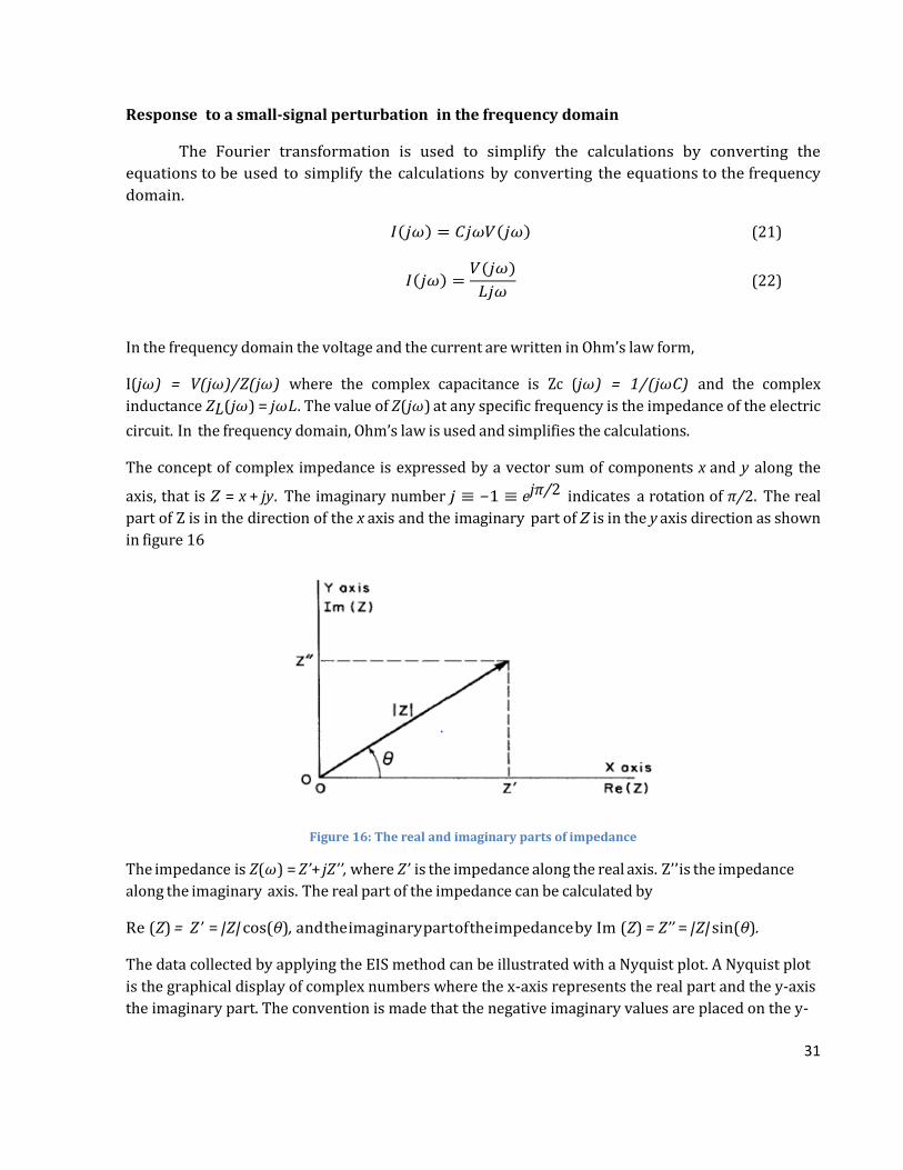
31

Response to a small-signal perturbation in the frequency domain

The Fourier transformation is used to simplify the calculations by converting the

equations to be used to simplify the calculations by converting the equations to the frequency

domain.

𝐼(𝑗𝜔) = 𝐶𝑗𝜔𝑉(𝑗𝜔)

(21)

𝐼(𝑗𝜔) =

𝑉(𝑗𝜔)

𝐿𝑗𝜔 (22)

In the frequency domain the voltage and the current are written in Ohm’s law form,

I(jω) = V(jω)/Z(jω) where the complex capacitance is Zc (jω) = 1/(jωC) and the complex

inductance ZL(jω) = jωL. The value of Z(jω) at any specific frequency is the impedance of the electric

circuit. In the frequency domain, Ohm’s law is used and simplifies the calculations.

The concept of complex impedance is expressed by a vector sum of components x and y along the

axis, that is Z = x + jy. The imaginary number j ≡ −1 ≡ ejπ/2 indicates a rotation of π/2. The real

part of Z is in the direction of the x axis and the imaginary part of Z is in the y axis direction as shown

in figure 16

Figure 16: The real and imaginary parts of impedance

The impedance is Z(ω) = Z’+ jZ’’, where Z’ is the impedance along the real axis. Z’’is the impedance

along the imaginary axis. The real part of the impedance can be calculated by

Re (Z) = Z’ = |Z| cos(θ), and the imaginary part of the impedance by Im (Z) = Z’’ = |Z| sin(θ).

The data collected by applying the EIS method can be illustrated with a Nyquist plot. A Nyquist plot

is the graphical display of complex numbers where the x-axis represents the real part and the y-axis

the imaginary part. The convention is made that the negative imaginary values are placed on the y-

32

axis as shown in figure. Each point on the plot is the complex impedance at the frequency at which

the impedance is measured. Figure shows a typical Nyquist plot.

Graph 4: Typical Nyquist Plot of PEM electrolyzer

The range of impedance is shown in a Nyquist plot. The behavior of the electrodes, membrane and

the electrode-membrane interfaces can be determined. The advantage of EIS is the ability to resolve,

in the frequency domain, the various losses associated with a PEM electrolyzer. The losses

include the ohmic, activation and mass transfer losses.

High frequency is shown at the left of the Nyquist plot and the low frequency is towards the right.

The high frequency semicircle reflects the activation resistance while the low frequency data always

reflects the mass transport limitations.

High frequency arc

The high frequency arc ranges from 200 kHz to 10 Hz. The intercept of the high frequency arc with

the real axis indicates the ohmic resistance. This is due to pure resistance which does not have an

imaginary part. Ohmic resistance is related to the resistance in the membrane and the conductors.

-0,015

-0,010

-0,005

0,000

0,005

0,010

0,015

0,000 0,005 0,010 0,015 0,020 0,025 0,030

Imag

inar

y I

mp

edan

ce (

Oh

m)(

-Zi)

Real Impedance (Ohm)(Zr)

Ohmic Losses

Anode Activation Losses Mass Transport Losses

Inductive Effect

High Frequency Low Frequency

33

Graph 5: Nyquist Plot - High frequency arc

The hydrogen evolution reaction (HER) takes place at the cathode. This reaction is faster than the

oxygen evolution reaction (OER) which takes place at the anode. The impedance spectrum of the

electrolyzer is almost equal to only the anode impedance. Many researchers use the impedance data

of the anode only, since the cathode impedance is negligible. If the kinetics of the HER is visible, two

overlapping semicircles are noticeable in the high frequencies (not seen in graph 5). The smaller

semicircle is due to the cathode activation resistance. The second semicircle is the anode activation

resistance. The diameter of the two semicircles represents the activation losses which includes the

membrane, GDL, bipolar plate and contact resistances. A change in this value during different

current densities is related to be the membrane hydration and the reaction kinetics of the reactions

at the anode and cathode.

Low frequency arc

Graph 6: Nyquist Plot - Low frequency arc

34

The low frequency region of a Nyquist plot can differ extremely depending on the operating current

density. Figure 6 shows the Nyquist plot of one current density. The low frequency region ranges

from 10 Hz to 0.01 Hz.

The most simplified behavior of the impedance spectrum is a single impedance semicircle. The

impedance spectra can shows a 45o line at low frequencies or the impedance can have a second

semicircle (as seen in graph 6). (Wagner, et al., 2004) identified these phenomena: If no diffusion is

present only one arc is present, if diffusion is present and if it is finite, two arcs are present (as in

this case) and if the diffusion is infinite a 450 straight line is present at the low frequency region. The

impedance spectra at low frequencies always reflect the impedance due to mass transport

limitations.

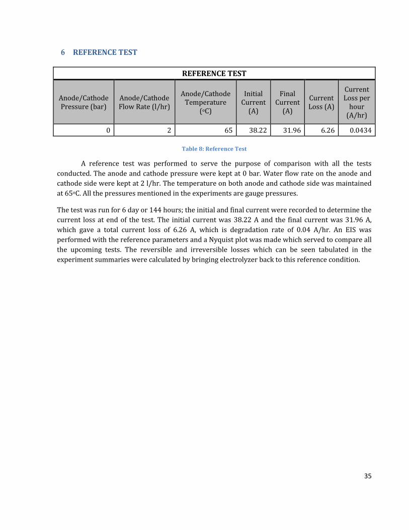
35

6 REFERENCE TEST

REFERENCE TEST

Anode/Cathode Pressure (bar)

Anode/Cathode Flow Rate (l/hr)

Anode/Cathode Temperature

(oC)

Initial Current

(A)

Final Current

(A)

Current Loss (A)

Current Loss per

hour (A/hr)

0 2 65 38.22 31.96 6.26 0.0434

Table 8: Reference Test

A reference test was performed to serve the purpose of comparison with all the tests

conducted. The anode and cathode pressure were kept at 0 bar. Water flow rate on the anode and

cathode side were kept at 2 l/hr. The temperature on both anode and cathode side was maintained

at 65oC. All the pressures mentioned in the experiments are gauge pressures.

The test was run for 6 day or 144 hours; the initial and final current were recorded to determine the

current loss at end of the test. The initial current was 38.22 A and the final current was 31.96 A,

which gave a total current loss of 6.26 A, which is degradation rate of 0.04 A/hr. An EIS was

performed with the reference parameters and a Nyquist plot was made which served to compare all

the upcoming tests. The reversible and irreversible losses which can be seen tabulated in the

experiment summaries were calculated by bringing electrolyzer back to this reference condition.

36

7 SINGLE PARAMETER TESTS

It is of immense interest, in an effort to study PEM electrolysis, to know how temperature, pressure,

water flow rate and current density affect the performance of an electrolyzer.

The effect of temperature and current density on electrolyzer has been widely studied, however

there aren’t detailed studies regarding the pressure and water flow rate. In the initial set of

experiments, these effects of pressure and water flow rate were investigated. These individual

effects were useful to understand the combined effects of pressure and water flow rate on the

performance, which helped identify the mechanisms causing the most degradation.

For the purpose of testing, the temperature set on both anode and cathode side was 65 oC. The

temperature was found by (Sun, et al., 2015) to be optimum for single electrolyzer cell of area 25

cm2 to be operated between flow rates of 0.3 to 2 l/hr flow rates (Lee, et al., 2013), also it was

observed by (Sun, et al., 2015) that operating PEM electrolyzer above 70 oC results in faster

softening of the gasket. Thus a temperature of 65 oC and water flow rate of 2 l/hr were selected to

perform the experiments. The operation of electrolyzer was potentiostatic and was set at 2 V.

7.1 CATHODE PRESSURIZATION TEST

The cathode side pressure was increased from 0 to 6 bar with an increase of 1 bar every 12 hours.

The readings of current and hydrogen % in oxygen were taken at an interval of 2 seconds. The

outcome of the experiment is summarized in the table 9 and graph 7.

Cathode Pressurization Test

Pressure (bar)

Hydrogen in Oxygen Stream (vol%)

Average Current (A)

Current Loss (A)

Current loss per hour (A)

0 6.03 44.26 4.66 0.38

1 6.74 39.59 3.71 0.31

2 7.34 35.88 3.07 0.25

3 7.86 32.80 3.03 0.25

4 8.13 29.76 1.86 0.15

5 8.29 27.90 1.80 0.15

6 8.34 26.10

Total 18.16 0.21

Table 9: Cathode Pressurization Test

One can see from the graph, an increase in the cathode pressure caused a subsequent fall in the

average current at each set of parameters. The total loss suffered in the entire experiment was 18.16

A; with a current loss rate of approximately 0.21 A/hr. After the EIS was done and the Nyquist plots

were made, the reversible and irreversible losses were identified; the irreversible loss was 18.19 A

with almost negligible reversible loss.

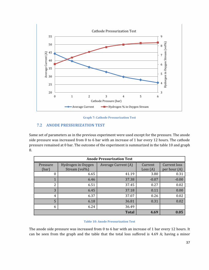
37

Graph 7: Cathode Pressurization Test

7.2 ANODE PRESSURIZATION TEST

Same set of parameters as in the previous experiment were used except for the pressure. The anode

side pressure was increased from 0 to 6 bar with an increase of 1 bar every 12 hours. The cathode

pressure remained at 0 bar. The outcome of the experiment is summarized in the table 10 and graph

8.

Anode Pressurization Test

Pressure (bar)


Average Current (A) Current Loss (A)


0 6.65 41.19 3.80 0.31

1 6.46 37.38 -0.07 -0.00

2 6.51 37.45 0.27 0.02

3 6.45 37.18 0.11 0.00

4 6.37 37.07 0.26 0.02

5 6.18 36.81 0.31 0.02

6 6.24 36.49

Total 4.69 0.05

Table 10: Anode Pressurization Test

The anode side pressure was increased from 0 to 6 bar with an increase of 1 bar every 12 hours. It

can be seen from the graph and the table that the total loss suffered is 4.69 A; having a minor

3

4

5

6

7

8

9

20

25

30

35

40

45

50

55

0 1 2 3 4 5 6

Hy

do

rgen

in O

xyge

n S

trea

m (

vo

l%)

Av

erag

e C

urr

ent

(A)

Cathode Pressure (bar)

Cathode Pressurization Test

Average Current Hydrogen % in Oxygen Stream

38

current loss rate of 0.05 A/hr. After completing the EIS and plotting the Nyquist plots, the

irreversible loss was found to be 22.29 A and reversible loss was -18 A. There is an initial loss of

current after increase to 1 bar, but after that the current stays almost constant with a slightly

decreasing trend. The hydrogen vol% decreases with increase in anode pressure, as the oxygen side

would restrict crossing over given the larger side of oxygen molecules. The anode pressurization

does not have a prominent effect on hydrogen crossover as it is more or less constant as seen in

graph 8.

Graph 8: Anode Pressurization Test

Theoretically it can be concluded from the Nernst equation that the cathode side pressure

(hydrogen) has a higher effect on performance as compared to the anode pressure. The same

conclusion was evident in the experimental results as well.

7.3 CATHODE FLOW RATE VARIATION

Most of the published studies do not vary cathode flow rate but just refill the cathode side by using a

replenishing reservoir, but since this setup has a separate pump for each side, we could vary the

flow rate and observe the effects.

This set of experiments was carried out to investigate the effect of water flow rate on electrolyzer

performance. The voltage was set at 2 V, anode and cathode side pressure was set at 0 bar and the

temperature on both sides was 65 oC. The same set of parameters was also used for anode flow rate

experiments.

3

4

5

6

7

8

9

20

25

30

35

40

45

50

55

0 1 2 3 4 5 6

Hy

do

rgen

in O

xyge

n S

trea

m (

vo

l%)

Av

erag

e C

urr

emt

(A)

Anode Pressure (bar)

Anode Pressurization Test

Average Current (A) Average Hydrogen % in Oxygen Stream

39

Cathode Flow Rate Variation

Anode flow rate (l/hr)

Cathode flow rate (l/hr)

Average Current (A)


Current Loss (A)


2.0 0.2 39.17 6.01 0.64 0,05

2.0 0.6 36.80 6.04 2.10 0,17

2.0 0.8 34.70 6.03 1.40 0,11

2.0 1.0 33.30 6.05 2.79 0,23

2.0 3.0 30.51 6.10 0.59 0,04

2.0 4.0 29.92 6.26 0.47 0,03

2.0 5.0 29.45 6.17 1.22 0,10

2.0 6.0 28.23 6.23

Total 10.94 0.11

Table 11: Cathode Flow Rate Variation

The cathode flow rate variation started with 0 l/hr and stepping up by 0.2 l/hr every 12 hours.

There was jump from 1 l/hr to 3 l/hr as the test bench usually runs at 2 l/hr. The resultant was a

loss of 10.94 A which translates to a loss rate of 0.11 A/hr which is not that significant.

As seen in graph 9, there is initial decline in current with increase in the flow rates till 1 l/hr. There

is no considerable loss of current for the final four flow rates.

Graph 9: Cathode Flow Rate Variation

20

25

30

35

40

45

50

55

0,0 0,5 1,0 1,5 2,0 2,5 3,0 3,5 4,0 4,5 5,0 5,5 6,0

Av

erag

e C

urr

ent

(A)

Cathode Flow Rate (l/hr)

Cathode Flow Rate Variation

Average Current

40

7.4 ANODE FLOW RATE VARIATION

The water flow is more relevant in anode as water is a participant in anode side reaction whereas

on the cathode side goes through hydrogen ions reacting with electrons to release hydrogen.

The anode flow rate variation started with 0 l/hr and stepping up by 0.2 l/hr every 12 hours. The

resultant was a loss of 23.87 A which translates to a loss rate of 0.27 A/hr. Post completion of EIS

and the Nyquist plots, the reversible loss of -2.95 A and irreversible loss of 26.82 were derived.

Anode Flow Rate Variation

Anode flow rate (l/hr)

Cathode flow rate (l/hr)

Average Current (A)


Current Loss (A)


0.2 2.0 55.74 6.55 4.18 0.34

0.6 2.0 51.56 6.29 3.46 0.28

0.8 2.0 48.09 6.44 2.70 0.22

1.0 2.0 45.39 6.34 4.98 0.41

3.0 2.0 40.40 6.52 1.35 0.11

4.0 2.0 39.05 6.66 6.52 0.54

5.0 2.0 32.53 6.82 0.66 0.05

6.0 2.0 31.86 6.65

Total 23.87 0.24

Table 12: Anode Flow Rate Variation

As seen in the graph 9, initially the average current has a steep drop which later at higher flow rates

is more of a gradual drop. The hydrogen % in oxygen stream doesn’t show a significant change

throughout the duration of the experiment. The anode flow rate exhibits almost thrice the losses of

cathode flow rate variation.

41

Graph 10: Anode Flow Rate Variation

7.5 NYQUIST PLOTS – SINGLE PARAMETER TESTS

Graph 11 shows the Nyquist plot for the most degrading mechanisms of the pressure and flow rate experiments Though the ohmic and the anode/cathode activation losses are similar, the mass transport losses & pseudo inductive behavior due to cathode pressurization is visibly higher than anode flow rate variation. Table 13 summarizes the reversible and irreversible losses from the anode flow rate variation and the cathode pressurization test (the two most degrading single parameter tests). The impedance loss and the low frequency crossover give the comparative extent of mass transport losses as the ohmic and activation losses are almost similar.

20

25

30

35

40

45

50

55

0 0,5 1 1,5 2 2,5 3 3,5 4 4,5 5 5,5 6

Av

erag

e C

urr

ent

(A)

Anode Flow Rate (l/hr)


Average Current (A)

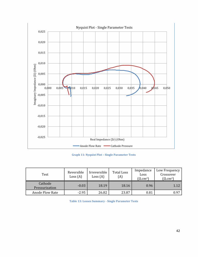
42

Graph 11: Nyquist Plot – Single Parameter Tests

Test Reversible

Loss (A) Irreversible

Loss (A) Total Loss

(A)

Impedance Loss

(Ω.cm2)

Low Frequency Crossover

(Ω.cm2)

Cathode Pressurization

-0.03 18.19 18.16 0.96 1.12

Anode Flow Rate -2.95 26.82 23.87 0.81 0.97

Table 13: Losses Summary - Single Parameter Tests

-0,025

-0,020

-0,015

-0,010

-0,005

0,000

0,005

0,010

0,015

0,020

0,025

0,000 0,005 0,010 0,015 0,020 0,025 0,030 0,035 0,040 0,045 0,050

Imag

inar

y I

mp

edan

ce (

Zi)

(O

hm

)

Real Impedance (Zr) (Ohm)

Nyquist Plot - Single Parameter Tests

Anode Flow Rate Cathode Pressure

43

8 COMBINATION TESTS

After investigating the effect of pressure and water flow rate individually, further studies were done

by varying the pressure and water flow rate in various combinations. These combination tests were

done in attempt to find which set of parameters degraded electrolyzer to the highest extent.

Eight combination tests were performed. In every combination test, six pairs of parameters were

tested, with each set lasting for 8 hours, thus a cumulative testing time of 48 hours per combination

test. In a similar fashion to previous experiments, after each and every combination test, EIS was

done and Nyquist plots were made. All the EIS were conducted with same set of parameters for the

purpose of being comparable and also so that the irreversible and reversible losses could be

separated from the total loss. The table below summarizes the combination set while testing and the

order of their variation. Green color indicates increasing order and red is decreasing order.

Combination Test Variables

Combination Test 1 Cathode Pressure Cathode Water Flow Rate

Combination Test 2 Anode Pressure Anode Water Flow Rate

Combination Test 3 Cathode Pressure Cathode Water Flow Rate

Combination Test 4 Anode Pressure Anode Water Flow Rate

Combination Test 5 Cathode Pressure Anode Water Flow Rate

Combination Test 6 Anode Pressure Cathode Water Flow Rate

Combination Test 7 Cathode Pressure Anode Water Flow Rate

Combination Test 8 Anode Pressure Cathode Water Flow Rate

Order of Variation Increasing Order Decreasing Order

Table 14: Combination Test Variables

Graphs and tables of average current and hydrogen vol% in oxygen volume against the varying

parameters of every combination test were plotted. After completion of all the eight combination

tests, it was identified that worst degrading tests were combination test 2 and 5. The tables and

graphs of these two tests are discussed below, whereas the data of rest of combination tests can be

found in the appendix.

44

8.1 COMBINATION TEST 2

The combination used in this test increased the anode pressure with increase in the anode flow rate.

The anode pressure was increased in steps of 1 bar from 1 to bar. The anode flow rate was

increased from 0.4 to 1.2 l/hr in steps of 0.4 l/hr followed by 3, 4 & 5 l/hr. The total loss incurred

during the tests was 9.49 A, of which 18.44 A was the irreversible loss and – 8.95 A was the

reversible loss as derived from the table 15 and the Nyquist plots i.e. graph 15. The total loss is

smaller than the irreversible loss as the reversible loss is negative; these losses were calculated by

bringing the electrolyzer to reference condition and the current recorded at the reference condition

was used as reference to determine the said losses. This was done for all tests to maintain

comparability.

Combination Test 2

Anode Pressure

(bar)


Hydrogen in Oxygen Stream

(vol%)

Average Current (A)

Current Loss (A)

Current Loss per hour (A/hr)

1 0.4 3.30 49.50 2.19 0.27

2 0.8 3.20 47.31 3.75 0.47

3 1.2 3.12 43.56 3.11 039

4 3.0 3.02 40.45 0.07 0.01

5 4.0 2.69 40.38 0.37 0.05

6 5.0 2.56 40.01

Total 9.49 0.20

Table 15: Combination Test 2

The above graph shows the behavior of average current (A) and hydrogen in oxygen (vol%) against

the anode flow rate. As one can see, the initial fall of current was steep which then went on to be

almost constant for the last three anode flow rates, giving a total loss of 9.49 A. It can be seen from

graph 13 that hydrogen in oxygen (vol%) throughout the experiment showed only a minor decrease

of 0.7 vol%.

The above graph shows the behavior of average current (A) and hydrogen in oxygen (vol%) against

the anode pressure. As one can see, the initial fall of current was steep which then went on to be

almost constant for the last three anode flow rates, giving a total loss of 9.49 A. It can be fairly

concluded from the graph that hydrogen in oxygen (vol%) throughout the experiment showed only

a minor decrease of 0.7 vol%.

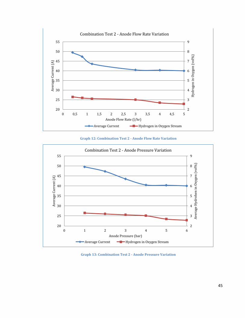
45

Graph 12: Combination Test 2 - Anode Flow Rate Variation

Graph 13: Combination Test 2 - Anode Pressure Variation

2

3

4

5

6

7

8

9

20

25

30

35

40

45

50

55

0 0,5 1 1,5 2 2,5 3 3,5 4 4,5 5

Hy

dro

gen

in O

xyge

n (

vo

l%)

Av

erag

e C

urr

ent

(A)


Combination Test 2 - Anode Flow Rate Variation

Average Current Hydrogen in Oxygen Stream

2

3

4

5

6

7

8

9

20

25

30

35

40

45

50

55

0 1 2 3 4 5 6

Av

erag

e H

yd

roh

en in

Oxy

gen

(v

ol%

)

Av

erag

e C

urr

ent

(A)


Combination Test 2 - Anode Pressure Variation


46

8.2 COMBINATION TEST 5

The combination used in this test is increase in cathode pressure with increase in anode flow rate.

As seen in the individual test, cathode pressure and anode flow rate variation were the most

degrading mechanisms. Evidently so, combining them together yielded the highest total current loss

amongst all other combination tests.

As one can see in the table 17, the total loss suffered during combination test 5 was 22.43 A, of

which 12 A was the irreversible loss and 10.40 A was the reversible loss. It can be observed from

the graph that there was steep drop in current during the three initial set of parameters and a rather

gradual on at higher anode flow rates and cathode pressure.

Combination Test 5




(vol%)

Average Current (A)

Current Loss (A)


1 0.4 4.65 52.39 5.86 0.73

2 0.8 5.13 46.53 3.86 0.48

3 1.2 5.40 42.67 5.34 0.67

4 3.0 5.64 37.33 2.38 0.30

5 4.0 5.78 34.95 1.86 0.23

6 5.0 6.05 33.09 Total 19.30 0.40


Graph 14 shows the behavior of average current (A) and hydrogen in oxygen (vol%) against the

anode flow rate. As one can see, the initial fall of current was steep which then went on to be a

gradual decrease. It can be concluded that the current change in flow rates in higher orders above 2

l/hr are gradual.

For flow rates lower than 2 l/hr, the decrease in average current can be represented by linear line

fit y = -12,161x + 56,929 and for flow rates higher than 2 l/hr it is y = -2,117x + 43,595. Such trend

was approximately followed by average current against anode flow rate variation, suggesting faster

degradation at lower flow rates compared to higher flow rates. Graph 14 also shows that hydrogen

in oxygen (vol%) has a rapid increase initially which then became more gradual, it follows the same

trend as average current but in opposite manner.


cathode pressure. As one can see, the fall of current was constant with increase in pressure, with the

nature of the slope decreasing slightly towards the end.

47


Graph 15: Combination Test 5 - Cathode Pressure Variation

Graph 15 showed that hydrogen in oxygen (vol%) has a rather constant increase with cathode

pressure. It reinforces the observation made in the cathode pressurization test with both tests

having increase of approximately 2 vol% in hydrogen in oxygen.

2

3

4

5

6

7

8

9

20

25

30

35

40

45

50

55

0 0,5 1 1,5 2 2,5 3 3,5 4 4,5 5

Hy

dro

gen

in O

xyge

n (

vo

l%)

Av

erag

e C

urr

ent

(A)


Combination Test 5 - Anode Flow Rate Variation


2

3

4

5

6

7

8

9

20

25

30

35

40

45

50

55

0 1 2 3 4 5 6

Hy

dro

gen

in O

xyge

n (

vo

l%)

Av

erag

e C

urr

ent

(A)


Combination Test 5 - Cathode Pressure Variation


48

8.3 NYQUIST PLOTS - COMBINATION TESTS

Test Variation

Type Reversible

Loss (A) Irreversible

Loss (A)

Total Loss (A)

Impedance Loss

(Ω.cm2)


(Ω.cm2)

Combination Test 1 CP CFR 6.31 11.88 18.18 0.56 0.71

Combination Test 2 AP AFR -8.95 18.43 9.48 0.69 0.86

Combination Test 3 CP CFR -1.31 17.82 6.51 0.59 0.74

Combination Test 4 AP AFR -8.50 7.36 -2.14 0.62 0.78

Combination Test 5 CP AFR 10.42 12.02 22.44 0.37 0.50

Combination Test 6 AP CFR -6.98 12.14 5.16 0.50 0.65

Combination Test 7 CP AFR -0.80 2.51 1.71 0.44 0.58

Combination Test 8 AP CFR -8.14 5.93 -2.21 0.55 0.71

Cathode Pressurization -0.03 18.19 18.16 0.96 1.12

Anode Flow Rate -2.95 26.82 23.87 0.81 0.97

AP – Anode Pressure, CP – Cathode Pressure AFR – Anode Flow Rate, CFR – Cathode Flow Rate

Green Color – Increasing Trend Red Color – Decreasing Trend

Table 17: Combination Test Summary

Table 17 summarizes the total, irreversible & reversible losses along with impedance loss and low

frequency crossover seen in the Nyquist plots that occurred during all the combination tests and the

graph shows Nyquist plots of all the combination tests. It can be concluded that Combination Test 2

gives the most reversible degradation and Combination Test 5 gives the most irreversible

degradation.

After relating the typical Nyquist plot from EIS chapter to the Nyquist plots of the combination tests,

it is fair to say that the ohmic losses, the anode activation losses are identical but the mass transport

losses show significant differences.

49

Graph 16: Combination Tests - Nyquist Plot

From the Nyquist plot, it is seen that combination test 2 gives the most severe degradation, given

that the mass transport losses occurring as a result of increase in anode flow rate and anode side

pressure are most significant. In the table listing the losses incurred during the combination tests,

we can see that combination tests 1, 2 and 5 have the highest loss in current amongst the others.

Combination test 5 gives highest irreversible loss and 2 gives the highest reversible loss, this can be

attributed to the observation that anode flow rate causes more reversible loss and cathode

pressurization causes more irreversible loss.

-0,02

-0,015

-0,01

-0,005

0

0,005

0,01

0,015

0,02

0,000 0,005 0,010 0,015 0,020 0,025 0,030 0,035 0,040

Imag

inar

y I

mp

edan

ce (

Oh

m)

Real Impedance (Ohm)

Combination Tests - Nyquist Plot

Combination Test 1 Combination Test 2 Combination Test 3 Combination Test 4

Combination Test 5 Combination Test 6 Combination Test 7 Combination Test 8

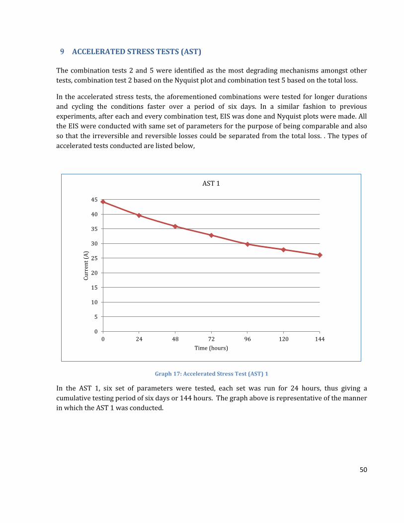
50

9 ACCELERATED STRESS TESTS (AST)

The combination tests 2 and 5 were identified as the most degrading mechanisms amongst other

tests, combination test 2 based on the Nyquist plot and combination test 5 based on the total loss.

In the accelerated stress tests, the aforementioned combinations were tested for longer durations

and cycling the conditions faster over a period of six days. In a similar fashion to previous

experiments, after each and every combination test, EIS was done and Nyquist plots were made. All

the EIS were conducted with same set of parameters for the purpose of being comparable and also

so that the irreversible and reversible losses could be separated from the total loss. . The types of

accelerated tests conducted are listed below,

Graph 17: Accelerated Stress Test (AST) 1

In the AST 1, six set of parameters were tested, each set was run for 24 hours, thus giving a

cumulative testing period of six days or 144 hours. The graph above is representative of the manner

in which the AST 1 was conducted.

0

5

10

15

20

25

30

35

40

45

0 24 48 72 96 120 144

Cu

rren

t (A

)

Time (hours)

AST 1

51

Graph 18: Accelerated Stress Test (AST) 2

In the AST 2, six set of parameters were tested, each set was run for 8 hours, and then the same set

was repeated. In this fashion, we tested 3 cycles over period of 6 days or 144 hours. The graph

above is representative of the manner in which the AST 2 was conducted.

0

5

10

15

20

25

30

35

40

45

0 8 16 24 32 40 48 56 64 72 80 88 96 104 112 120 128 136 144

Cu

rren

t (A

)

Time (hours)

AST 2

52

9.1 AST 1 CT 2

In this AST, the set of parameters used were that of combination 2 and the method of testing was

AST 1, hence the name AST 1 CT 2. The combination 2 used in this test increased the anode pressure

with increase in the anode flow rate. The anode pressure was increased in steps of 1 bar from 1 to 6

bar. The anode flow rate was increased from 0.4 to 1.2 l/hr in steps of 0.4 l/hr followed by 3, 4 & 5

l/hr. The average current and hydrogen % in oxygen stream were recorded and tabulated as below.

AST 1 CT 2

Anode Pressure

(bar)


Average Current (A)


(vol%)

Current Loss (A)


1 0.4 47.08 7.42 3.85 0.16

2 0.8 43.23 7.44 2.57 0.11

3 1.2 40.66 6.59 3.11 0.13

4 3.0 37.55 6.31 0.53 0.02

5 4.0 37.02 5.49 0.37 0.02

6 5.0 36.65 4.44

Total 10.43 0.07 Table 18: AST 1 CT 2

As one can see in table 18, the total loss suffered during the test was 10.43 A of which 21.57 A was

the irreversible loss and -11.14 A was the reversible loss. The hydrogen in oxygen stream gradually

decreases from 7.42 to about 4.44 vol% over the duration of the test.


anode pressure variation. As one can see, the fall of current was steep initially and gets flatter

towards the end. The decline in the hydrogen in oxygen (vol%) is almost gradual throughout the

test.

53

Graph 19: AST 1 CT 2 - Anode Pressure Variation

Graph 20: AST 1 CT 2 - Anode Flow Rate Variation


anode flow rate variation. As was the case with anode pressure variation, the fall of current was

steep for the smaller flow rates as compared to the higher flow rates.

3

4

5

6

7

8

9

20

25

30

35

40

45

50

55

0 1 2 3 4 5 6

Hy

dri

gen

in O

xyge

n S

trea

m (

vo

l%)

Av

erag

e C

urr

ent

(A)


Anode Pressure Variation


3

4

5

6

7

8

9

20

25

30

35

40

45

50

0 0,5 1 1,5 2 2,5 3 3,5 4 4,5 5

Hy

dro

gen

in O

xyge

n S

trea

m (

vo

l%)

Av

erag

e C

urr

ent

(A)




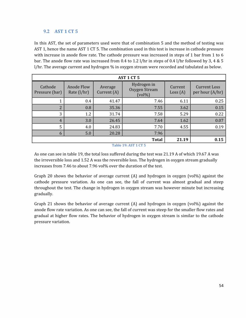
54

9.2 AST 1 CT 5

In this AST, the set of parameters used were that of combination 5 and the method of testing was

AST 1, hence the name AST 1 CT 5. The combination used in this test is increase in cathode pressure

with increase in anode flow rate. The cathode pressure was increased in steps of 1 bar from 1 to 6

bar. The anode flow rate was increased from 0.4 to 1.2 l/hr in steps of 0.4 l/hr followed by 3, 4 & 5

l/hr. The average current and hydrogen % in oxygen stream were recorded and tabulated as below.

AST 1 CT 5



Average Current (A)


(vol%)

Current Loss (A)


1 0.4 41.47 7.46 6.11 0.25

2 0.8 35.36 7.55 3.62 0.15

3 1.2 31.74 7.58 5.29 0.22

4 3.0 26.45 7.64 1.62 0.07

5 4.0 24.83 7.70 4.55 0.19

6 5.0 20.28 7.96

Total 21.19 0.15 Table 19: AST 1 CT 5

As one can see in table 19, the total loss suffered during the test was 21.19 A of which 19.67 A was

the irreversible loss and 1.52 A was the reversible loss. The hydrogen in oxygen stream gradually

increases from 7.46 to about 7.96 vol% over the duration of the test.


cathode pressure variation. As one can see, the fall of current was almost gradual and steep

throughout the test. The change in hydrogen in oxygen stream was however minute but increasing

gradually.


anode flow rate variation. As one can see, the fall of current was steep for the smaller flow rates and

gradual at higher flow rates. The behavior of hydrogen in oxygen stream is similar to the cathode

pressure variation.

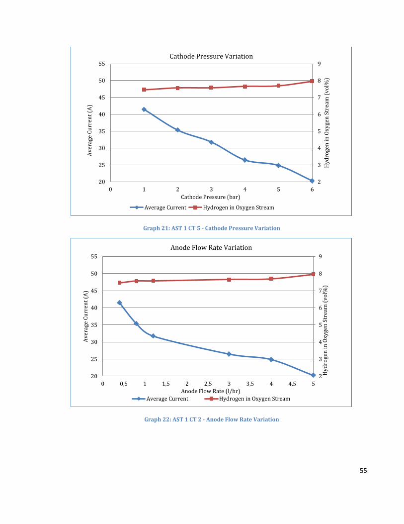
55

Graph 21: AST 1 CT 5 - Cathode Pressure Variation

Graph 22: AST 1 CT 2 - Anode Flow Rate Variation

2

3

4

5

6

7

8

9

20

25

30

35

40

45

50

55

0 1 2 3 4 5 6

Hy

dro

gen

in O

xyge

n S

trea

m (

vo

l%)

Av

erag

e C

urr

ent

(A)


Cathode Pressure Variation


2

3

4

5

6

7

8

9

20

25

30

35

40

45

50

55

0 0,5 1 1,5 2 2,5 3 3,5 4 4,5 5

Hy

dro

gen

in O

xyge

n S

trea

m (

vo

l%)

Av

erag

e C

urr

ent

(A)




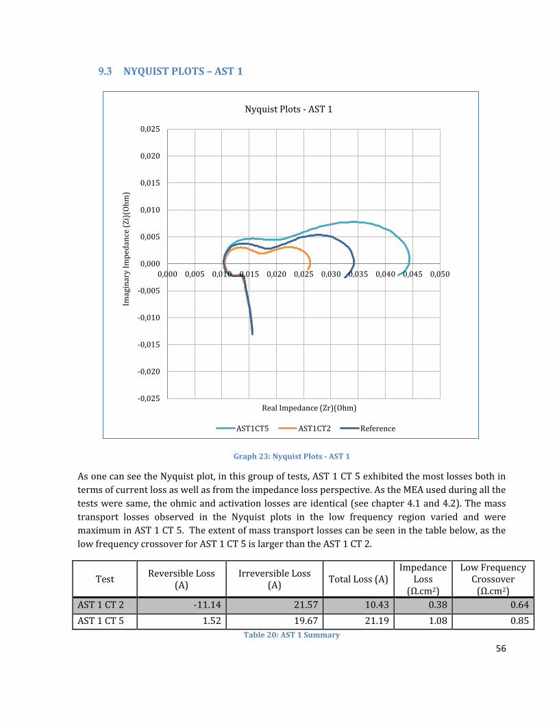
56

9.3 NYQUIST PLOTS – AST 1

Graph 23: Nyquist Plots - AST 1

As one can see the Nyquist plot, in this group of tests, AST 1 CT 5 exhibited the most losses both in

terms of current loss as well as from the impedance loss perspective. As the MEA used during all the

tests were same, the ohmic and activation losses are identical (see chapter 4.1 and 4.2). The mass

transport losses observed in the Nyquist plots in the low frequency region varied and were

maximum in AST 1 CT 5. The extent of mass transport losses can be seen in the table below, as the

low frequency crossover for AST 1 CT 5 is larger than the AST 1 CT 2.

Test Reversible Loss

(A) Irreversible Loss

(A) Total Loss (A)

Impedance Loss

(Ω.cm2)


(Ω.cm2)

AST 1 CT 2 -11.14 21.57 10.43 0.38 0.64

AST 1 CT 5 1.52 19.67 21.19 1.08 0.85

Table 20: AST 1 Summary

-0,025

-0,020

-0,015

-0,010

-0,005

0,000

0,005

0,010

0,015

0,020

0,025

0,000 0,005 0,010 0,015 0,020 0,025 0,030 0,035 0,040 0,045 0,050

Imag

inar

y I

mp

edan

ce (

Zi)

(Oh

m)

Real Impedance (Zr)(Ohm)

Nyquist Plots - AST 1

AST1CT5 AST1CT2 Reference

57

9.4 AST 2 CT 2

AST 2 CT 2



Average Current (A)


Cycle 1

1 0.4 46.50 4.91

2 0.8 45.45 4.59

3 1.2 44.81 4.63

4 3.0 42.13 4.50

5 4.0 41.27 4.32

6 5.0 39.27 4.34

Cycle 2

1 0.4 43.68 5.63

2 0.8 42.46 5.35

3 1.2 41.24 5.25

4 3.0 38.43 4.89

5 4.0 37.52 4.77

6 5.0 36.58 4.66

Cycle 3

1 0.4 39.51 5.37

2 0.8 38.94 5.22

3 1.2 37.75 5.20

4 3.0 35.65 5.01

5 4.0 35.24 4.83

6 5.0 34.16 4.81

Table 21: AST 2 CT 2

The AST 2 the parameters of CT 2 and 5 were cycled to observe the effect of cycling on the

performance. The data was recorded and tabulated as seen in table. It can be seen from the table

that the current loss through cycle 1 was 7.23 A, cycle 2 was 7.1 A and cycle 3 was 5.31 A. The

overall current loss after all the cycles was 12.34 A, giving a degradation rate of 0.08 A/hr. The

hydrogen vol% in oxygen stream decreases steadily in every cycle as the rise in anode pressure

restricts hydrogen from crossing over to anode side.

The graphs present the average current and hydrogen vol% in oxygen stream against anode

pressure and anode flow rate for each cycle carried out. As seen in all the graphs of this test, the

trend is identical. The average current and hydrogen vol% decreases gradually till completion of the

cycle.

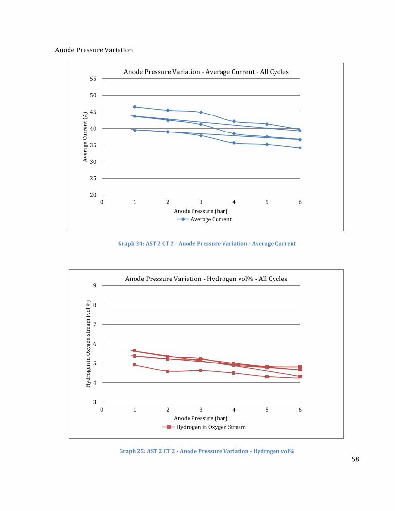
58

Anode Pressure Variation

Graph 24: AST 2 CT 2 - Anode Pressure Variation - Average Current

Graph 25: AST 2 CT 2 - Anode Pressure Variation - Hydrogen vol%

20

25

30

35

40

45

50

55

0 1 2 3 4 5 6

Av

erag

e C

urr

ent

(A)


Anode Pressure Variation - Average Current - All Cycles

Average Current

3

4

5

6

7

8

9

0 1 2 3 4 5 6

Hy

dro

gen

in O

xyge

n s

trea

m (

vo

l%)


Anode Pressure Variation - Hydrogen vol% - All Cycles


59


Graph 26: AST 2 CT 2 - Anode Flow Rate Variation - Average Current

Graph 27: AST 2 CT 2 - Anode Flow Rate Variation - Hydrogen vol%

20

25

30

35

40

45

50

55

0,0 0,5 1,0 1,5 2,0 2,5 3,0 3,5 4,0 4,5 5,0

Av

erag

e C

urr

ent

(A)


Anode Flow Rate Variation - Average Current - All Cycles

Average Current

3

4

5

6

7

8

9

0,0 0,5 1,0 1,5 2,0 2,5 3,0 3,5 4,0 4,5 5,0

Hy

dro

gen

in O

xyge

n S

trea

m (

vo

l%)


Anode Flow Rate Variation - Hydrogen vol% - All Cycles


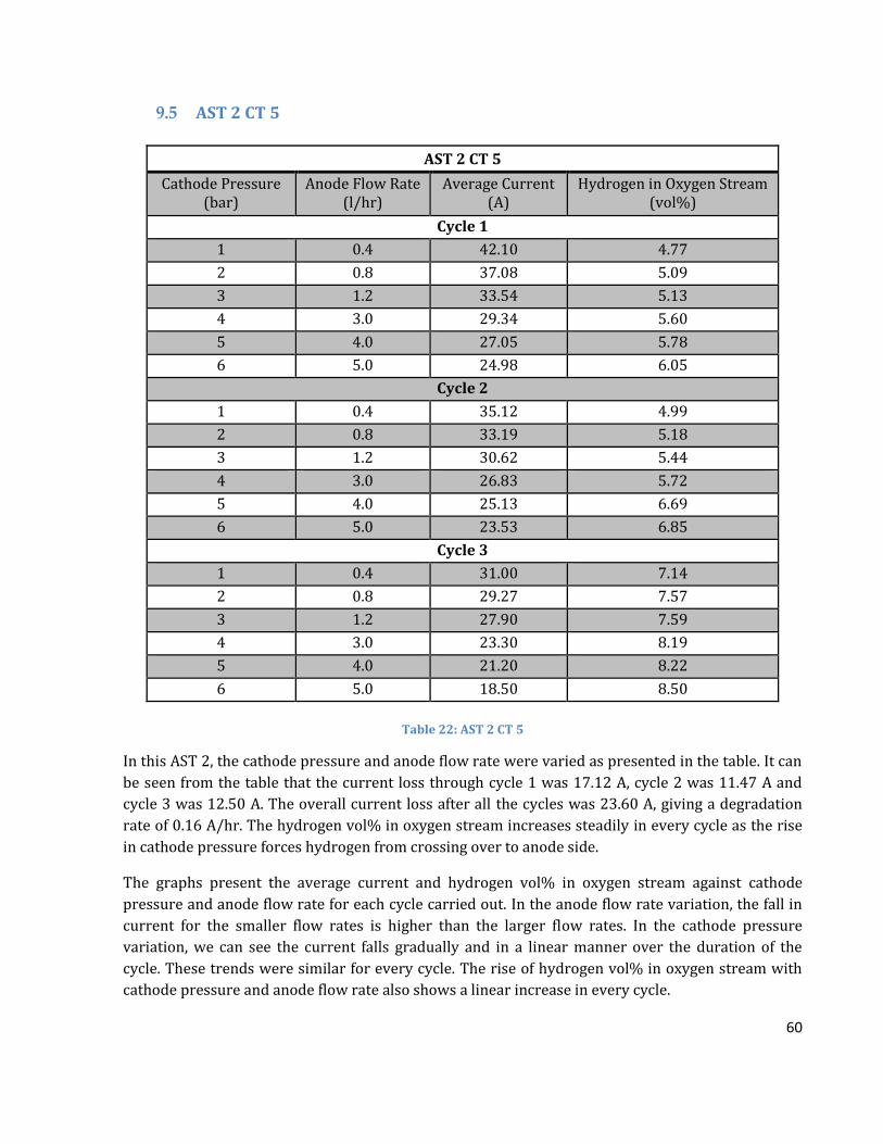
60

9.5 AST 2 CT 5

AST 2 CT 5



Average Current (A)


Cycle 1

1 0.4 42.10 4.77

2 0.8 37.08 5.09

3 1.2 33.54 5.13

4 3.0 29.34 5.60

5 4.0 27.05 5.78

6 5.0 24.98 6.05

Cycle 2

1 0.4 35.12 4.99

2 0.8 33.19 5.18

3 1.2 30.62 5.44

4 3.0 26.83 5.72

5 4.0 25.13 6.69

6 5.0 23.53 6.85

Cycle 3

1 0.4 31.00 7.14

2 0.8 29.27 7.57

3 1.2 27.90 7.59

4 3.0 23.30 8.19

5 4.0 21.20 8.22

6 5.0 18.50 8.50

Table 22: AST 2 CT 5

In this AST 2, the cathode pressure and anode flow rate were varied as presented in the table. It can

be seen from the table that the current loss through cycle 1 was 17.12 A, cycle 2 was 11.47 A and

cycle 3 was 12.50 A. The overall current loss after all the cycles was 23.60 A, giving a degradation

rate of 0.16 A/hr. The hydrogen vol% in oxygen stream increases steadily in every cycle as the rise

in cathode pressure forces hydrogen from crossing over to anode side.

The graphs present the average current and hydrogen vol% in oxygen stream against cathode

pressure and anode flow rate for each cycle carried out. In the anode flow rate variation, the fall in

current for the smaller flow rates is higher than the larger flow rates. In the cathode pressure

variation, we can see the current falls gradually and in a linear manner over the duration of the

cycle. These trends were similar for every cycle. The rise of hydrogen vol% in oxygen stream with

cathode pressure and anode flow rate also shows a linear increase in every cycle.

61

Cathode Pressure Variation

Graph 28: AST 2 CT 5 - Cathode Pressure Variation - Average Current

Graph 29: AST 2 CT 5 - Cathode Pressure Variation - Hydrogen vol%

15

20

25

30

35

40

45

50

55

0 1 2 3 4 5 6

Av

erag

e C

urr

ent

(A)


Cathode Pressure Variation - Average Current - All Cycles

Average Current

3

4

5

6

7

8

9

0 1 2 3 4 5 6

Hy

dro

gen

in O

xyge

n S

trea

m (

vo

l%)


Cathode Pressure Variation - Hydrogen vol% - All Cycles


62


Graph 30: AST 2 CT 5 - Anode Flow Rate Variation - Average Current

Graph 31: AST 2 CT 5 - Anode Flow Rate Variation - Hydrogen vol%

15

20

25

30

35

40

45

50

55

0,0 0,5 1,0 1,5 2,0 2,5 3,0 3,5 4,0 4,5 5,0

Av

erag

e C

urr

ent

(A)


Anode Flow Rate Variation - Average Current - All Cycles

Average Current

3

4

5

6

7

8

9

0,0 0,5 1,0 1,5 2,0 2,5 3,0 3,5 4,0 4,5 5,0

Hy

dro

gen

in O

xyge

n S

trea

m (

vo

l%)


Anode Flow Rate Variation - Hydrogen vol% - All Cycles


63

9.6 NYQUIST PLOTS – AST 2

Graph 32: Nyquist Plots - AST 2

As one can see the Nyquist plot, in this group of tests, AST 2 CT 5 exhibited the most losses both in

terms of current loss as well as from the impedance loss perspective. The mass transport losses

observed in the Nyquist plots in the low frequency region varied and were maximum in AST 2 CT 5.

AST 2 CT 5 showed more damage than AST 1 CT 5, thus cycling the parameters for the same time

frame has more degrading effect than maintaining same set of parameters for a longer period of

time. Since cycling is more effective, the test protocol can be carried out faster.

Test Reversible Loss

(A) Irreversible Loss

(A) Total Loss

(A)

Impedance Loss

(Ω.cm2)


(Ω.cm2)

AST 2 CT 2 3.93 8.41 12.34 0.21 0.35

AST 2 CT 5 3.42 20.19 23.60 0.92 0.64

Table 23: AST 2 summary

-0,020

-0,015

-0,010

-0,005

0,000

0,005

0,010

0,015

0,020

0,000 0,005 0,010 0,015 0,020 0,025 0,030 0,035 0,040

Imag

iner

y I

mp

edan

ce (

Oh

m)(

-Zi)

Real Impedance (Ohm)(Zre)

AST 2 - Nyquist Plots

AST2CT2

AST2CT5

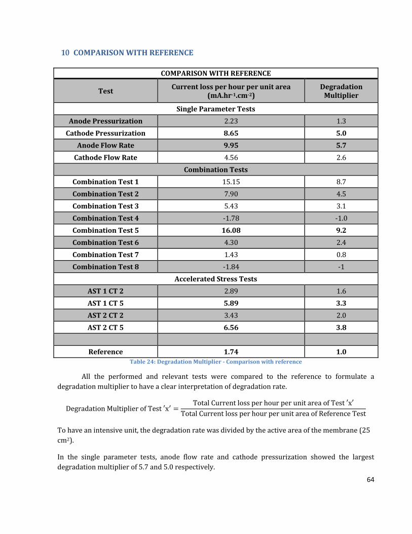
64

10 COMPARISON WITH REFERENCE

COMPARISON WITH REFERENCE

Test Current loss per hour per unit area

(mA.hr-1.cm-2) Degradation

Multiplier

Single Parameter Tests

Anode Pressurization 2.23 1.3

Cathode Pressurization 8.65 5.0

Anode Flow Rate 9.95 5.7

Cathode Flow Rate 4.56 2.6

Combination Tests

Combination Test 1 15.15 8.7



Combination Test 4 -1.78 -1.0




Combination Test 8 -1.84 -1

Accelerated Stress Tests

AST 1 CT 2 2.89 1.6

AST 1 CT 5 5.89 3.3

AST 2 CT 2 3.43 2.0

AST 2 CT 5 6.56 3.8

Reference 1.74 1.0

Table 24: Degradation Multiplier - Comparison with reference

All the performed and relevant tests were compared to the reference to formulate a

degradation multiplier to have a clear interpretation of degradation rate.

Degradation Multiplier of Test ′x′ =Total Current loss per hour per unit area of Test ′x′

Total Current loss per hour per unit area of Reference Test

To have an intensive unit, the degradation rate was divided by the active area of the membrane (25

cm2).

In the single parameter tests, anode flow rate and cathode pressurization showed the largest

degradation multiplier of 5.7 and 5.0 respectively.

65

In the combination tests, combination test 5 showed the highest degradation multiplier of 9.2 and in

the accelerated stress tests AST 2 CT 5 and AST 1 CT 5 showed the highest degradation multiplier of

3.8 and 3.3.

Combination test 5 has the highest degradation multiplier of 9.2 amongst all the tests. It can be

concluded from this that cycling of parameters has more degrading effect than time on the PEM

electrolyzer. It can also be concluded, that even though time doesn’t have considerable effect on

total loss or the degradation rate, it does increase the irreversible losses. From the table, we can see

that combination test 5 had a total loss of 19.30 A of which 12.01 A were irreversible and 7.26 A

reversible losses. Whereas, AST 1 CT 5 had a total loss of 21.19 A of which 19.67 A were irreversible

and 1.52 A reversible losses; AST 2 CT 5 had a total loss of 23.60 A of which 20.19 A were

irreversible and 3.42 A reversible losses.

66

11 CONCLUSIONS

From the single parameter tests, it can be concluded that increase in cathode pressure has a

more degrading effect than increase in anode pressure. The degree of influence or the degradation

multiplier was calculated and it can be seen that cathode pressure has almost 4 times more

degrading effect than anode pressure. This loss has been attributed to the hydrogen permeation.

(Trinke, et al., 2017) have studied the effects of increase in cathode pressure at 600C in pressure

range of 1-31 bar with respect to the current density.

The effect of anode flow rate shows higher degradation than the cathode flow rate. Ideally only the

anode is supplied with forced water flows and cathode is kept hydrated by natural convection of a

water reservoir. The increase in anode flow rate degrades the electrolyzer more than 2 times faster

than cathode flow rate. The anode flow rate has been attributed to bubble size and detachment

which is one of the reasons for mass transport losses (Suermann, et al., 2015).

The combination tests, helped conclude that the cathode pressure and anode flow rate together

caused the maximum damage to the electrolyzer. Thus operating them at higher cathode pressure

and anode flow rate is most degrading parameters at a fixed temperature. The degradation

multiplier of this combination being 9.2, it can be rightly used as a testing protocol to test against.

To optimize use of the combination for testing, it was useful to observe whether cycling or

lengthening the duration of the parameters caused more degradation. It was concluded that cycling

the parameters gives a higher total current loss as compared to lengthening the test. It is thus

beneficial that the testing protocol can be run faster by cycling the parameters for a given duration

of time. The duration was concluded to contribute more to the reversible current losses than the

irreversible losses.

Cathode Pressure

Anode Flow Rate

Figure 17: Most Degrading Combination

67

Having quantified the current loss, it was interesting to see the type of losses on the Nyquist plots.

As seen in the Nyquist plots of the single parameter tests, the combination tests and the ASTs, the

ohmic and activation losses are more or less similar for all the tests. The ohmic losses are attributed

to the MEA used and since it was the same for all the tests, the ohmic losses are the same. The

activation losses are attributed to the electro catalysts and MEA, thus they show similar losses as

well.

The losses that significantly vary over all the tests are the mass transport losses. The mass transport

losses due to reactants and products are seen in the low frequency region of the Nyquist plot as

mentioned before and these observations can be used to optimize the structure of current collectors

and MEAs as well. These effects have to be investigated further and in detail to isolate the losses

between the reactants and products and the subsequent effect of mass transport.

Figure 18: Relative Contribution of Losses at a) 1 bar and b) 100 bar balanced pressure

Even if the mechanism of the mass transport losses is not well understood, its contribution of

to the total overpotential is considerable. (Suermann, et al., 2015) showed in figure 18 the

relative contributions of the different as well as the Faraday losses due to gas crossover are

plotted as function of current density for 1 and 100 bar balanced pressure. Even if the mass

transport losses are almost independent of pressure, the relative contribution increases slightly

with increasing the pressure due to lower kinetic losses as a result of higher thermodynamic

voltages. Figure 18 shows that above of 1 A/cm2 mass transport losses contribute between 20 and

25 % to the total overpotential, both for 1 bar (18a) and 100 bar (18b). The Faraday losses due

to crossover are important at current densities below 1 A/cm2 and high pressure.

68

12 FUTURE OUTLOOK

The commercial operational range of a PEM electrolyzer is 1 to 2 A/cm2, which is slated to

increase further to make the electrolyzer more compact and deliver better performances. All the

detailed studies that have been done so far have been below 1 A/cm2, this demands for the future

work to be done in higher current density range so that there is a better understanding of the

behavior at practical higher current densities.

The frequency range of EIS usually performed has also been limited till 5 to 10 Hz in low frequency

range in most of the studies, and it has been conclusively seen that it does not represent all the

losses (I have conducted it till 10 mHz and the losses are more apparent). Thus more low frequency

studies are required showing the complete range of losses, which can go on further in achieving

better modelling for the PEM electrolyzer.

Also as mentioned before, there are limited studies done so far explaining the mechanisms of mass

transport and the responsible species and related effects. This study can be used as base for

modeling the mass transport by analyzing the EIS data for various operating conditions.

69

13 APPENDIX

13.1 HYDROGEN CROSSOVER TEST

A set of tests were carried out to investigate the effect of increasing cathode pressure on

hydrogen crossover. It was done with electrochemical impedance spectroscopy and an attempt was

made to explain the pseudo inductive behavior in the low frequency range. Evidence was found

showing a relationship between surface relaxation, Nernst impedance and hydrogen crossover.

The pressure was set at 0 bar on anode side, temperature on both anode and cathode side was kept

at 65 0C and the water flow rate was set at 2 l/hr. The cathode pressure was kept at 0, 3, 6 and 9 bar

while performing the EIS. The figure shows the model used for the tests.

Figure 19: EIS Model

EIS MODEL ELEMENTS

1 Inductor

2 Resistor (electrolyte)

3 Resistor (H2 reaction)

4 Capacitor (cathode)

5 Surface relaxation parameter

6 Resistor (O2 reaction)

7 Nernst impedance parameter

8 Capacitor (anode)

Table 25: EIS Model Elements

The inductor (1) and resistor (2) represent the ohmic losses in the electrolyzer cell dominated by

losses in the membrane. The adjoining resistor (3) and capacitor (4) represent the cathode

activation losses; these losses are negligible because the hydrogen evolution reaction at the cathode

is quite rapid, thus the losses are usually ignored. The next resistor (6) and Nernst impedance

parameter (7) with surface relaxation (5) in parallel with a capacitor (8); these represent the anode

activation (6 and 8) and mass transport losses (7). The following table and graph establish a relation

between Nernst impedance parameter, surface relaxation and hydrogen crossover.

70

Graph 33: Nyquist Plot - Hydrogen Crossover Test

HYDROGEN CROSSOVER TEST

Cathode Pressure 0 3 6 9 bar

EIS data

Inductance 1.789E-07 1.716E-07 1.795E-07 1.982E-07 H

Resistance (electrolyte) 0.006610 0.006735 0.006960 0.007301 Ohm

Resistance (H2 reaction) 0.006952 0.007017 0.007597 0.007170 Ohm

Capacitance (cathode) 0.1733 0.1738 0.1647 0.1687 F

CPE exponent (cathode) 1.100 1.118 1.121 1.160 -

Surface relaxation time 38.89 28.46 22.00 16.93 s

Surface relaxation resistance 0.004089 0.004381 0.004813 0.005100 Ohm

Resistance (O2 reaction) 0.009622 0.009199 0.009444 0.008503 Ohm

Nernst impedance Parameter 0.01662 0.02252 0.02449 0.02952 Ohm.s-1/2

Nernst impedance constant 3.214 2.476 2.786 2.029 s-1

Capacitance (anode) 0.6738 0.6268 0.6210 0.5459 F

CPE exponent (anode) 0.8549 0.9074 0.9245 1.0010 -

Test bench data

H2 vol% in O2 0.51 0.54 0.58 0.64 vol% Table 26: Hydrogen Crossover Test

-0,025

-0,020

-0,015

-0,010

-0,005

0,000

0,005

0,010

0,015

0,020

0,025

0,000 0,005 0,010 0,015 0,020 0,025 0,030 0,035 0,040 0,045 0,050

Imag

inar

y I

mp

edan

ce (

Oh

m)

Real Impedance (Ohm)

Hydrogen Crossover Test - Nyquist Plot

0 barg cathode

3 barg cathode

6 barg cathode

9 barg cathode

71

Graph 34: EIS vs Cathode Pressure

Graph 35: EIS vs Hydrogen vol%

As one can see from the table and the graph, hydrogen vol% in oxygen increases with increasing

cathode pressure. The hydrogen vol% in oxygen started with 0.51 % at 0 bar and rose steadily to

0.64 % at 9 bar, the increase had an almost linear trend.

0,000

0,005

0,010

0,015

0,020

0,025

0,030

0

0,001

0,002

0,003

0,004

0,005

0,006

0,007

0 1 2 3 4 5 6 7 8 9

Ner

nst

Im

ped

ance

Par

amet

er (

Oh

m.s

-1/2

)

Surf

ace

Rel

axat

ion

Res

ista

nce

(O

hm

)


EIS parameters vs Cathode Pressure

Surface Relaxation Impedence Nernst Impedance Parameter

0,50

0,52

0,54

0,56

0,58

0,60

0,62

0,64

0,66

0 1 2 3 4 5 6 7 8 9

Hy

dro

gen

vo

l% in

Oxy

gen


Hydrogen volume % in Oxygen

72

The Nyquist plots were fitted to the model depicted in the figure. After EIS was performed at each

pressure, values of the subsequent model parameters were compared, specifically Nernst

impedance parameter and surface relaxation resistance.

From the graph it can be observed that Nernst impedance parameter increases with the cathode

pressure. It rises from 0.01662 Ohm.s-1/2 at 0 bar to 0.02952 Ohm.s-1/2 at 9 bar in a non-linear

manner.

The Nernst impedance parameter characterizes the finite-length diffusion of the charge transfer

resistance and signifies the impedance contribution of the diffusion process. (Wagner, et al., 2004).

It can be seen that increase in hydrogen crossover corresponds to an increase in Nernst impedance

parameter, which in turns means that the impedance contribution of the diffusion process increases

resulting in higher mass transport losses which was evident in the Nyquist plots in graph 36.

One can see from the graph that the surface relaxation resistance increases with the cathode

pressure; it rose from 0.01662 Ohm.s-1/2 at 0 bar to 0.02952 Ohm.s-1/2 at 9 bar in a linear manner.

Surface relaxation refers to the availability of active area for the oxygen evolution reaction to take

place. The increase in crossover of hydrogen to the anode side makes it highly probable to hinder

the oxygen evolution reaction. It means there is a decrease in active area there by increasing the

surface relaxation resistance. If hydrogen meets the catalyst at the triple phase boundary, it will get

oxidized thereby competing directly with water electrolysis. The surface relaxation resistance

emulates the hydrogen cross over effect to a closer extent. The probability of competition increases

with hydrogen crossover rate, which was detected in EIS spectra as rise in the low frequency

pseudo-inductive behavior.

As seen in Nyquist plot, the low frequency pseudo-inductive behavior increased with the increase in

cathode pressure. Thus it can be concluded that an increase in cathode pressure causes rise in

hydrogen crossover which was seen in Nyquist plots as rise in low frequency pseudo-inductive

behavior explained with help of EIS model as increase in Surface relaxation and Nernst impedance

parameters.

73

13.2 COMBINATION TESTS

Combination Test 1




Average Current (A)

1 0.4 4.78 47.57

2 0.8 4.70 42.27

3 1.2 4.69 37.82

4 3.0 5.13 33.98

5 4.0 4.62 31.72

6 5.0 4.77 29.39


Graph 36: Combination Test 1 - Cathode Flow Rate Variation


2

3

4

5

6

7

8

20

25

30

35

40

45

50

55

0 0,5 1 1,5 2 2,5 3 3,5 4 4,5 5

Hy

dro

gen

in O

xyge

n S

trea

m (

vo

l%)

Av

erag

e C

urr

ent

(A)


Average Current


2

3

4

5

6

7

8

20

25

30

35

40

45

50

55

0 1 2 3 4 5 6

Hy

dro

gen

in O

xyge

n S

trea

m (

vo

l%)

Av

erag

e C

urr

ent

(A)


Average Current


74

Combination Test 3




Average Current (A)

1 5.0 7.51 42.77

2 4.0 7.50 39.49

3 3.0 7.54 37.62

4 1.2 7.48 38.79

5 0.8 7.44 37.60

6 0.4 7.49 36.26




2

3

4

5

6

7

8

20

25

30

35

40

45

50

55

0 0,5 1 1,5 2 2,5 3 3,5 4 4,5 5

Hy

dro

gen

in O

xyge

n S

trea

m (

vo

l%)

Av

erag

e C

urr

ent

(A)


Average Current


2

3

4

5

6

7

8

20

25

30

35

40

45

50

55

0 1 2 3 4 5 6

Hy

dro

gen

in O

xyge

n S

trea

m (

vo

l%)

Av

erag

e C

urr

ent

(A)


Average Current


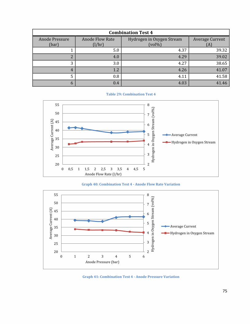
75

Combination Test 4




Average Current (A)

1 5.0 4.37 39.32

2 4.0 4.29 39.02

3 3.0 4.27 38.65

4 1.2 4.26 41.07

5 0.8 4.11 41.58

6 0.4 4.03 41.46




2

3

4

5

6

7

8

20

25

30

35

40

45

50

55

0 0,5 1 1,5 2 2,5 3 3,5 4 4,5 5

Hy

dro

gen

in O

xyge

n S

trea

m (

vo

l%)

Av

erag

e C

urr

ent

(A)


Average Current


2

3

4

5

6

7

8

20

25

30

35

40

45

50

55

0 1 2 3 4 5 6

Hy

dro

gen

in O

xyge

n S

trea

m (

vo

l%)

Av

erag

e C

urr

ent

(A)


Average Current


76

Combination Test 6




Average Current (A)

1 0.4 3.90 46.39

2 0.8 3.79 45.68

3 1.2 3.78 44.82

4 3.0 3.73 42.39

5 4.0 3.59 41.75

6 5.0 3.62 41.18




2

3

4

5

6

7

8

20

25

30

35

40

45

50

55

0 0,5 1 1,5 2 2,5 3 3,5 4 4,5 5

Hy

dro

gen

in O

xyge

n S

trea

m (

vo

l%)

Av

erag

e C

urr

ent

(A)


Average Current


2

3

4

5

6

7

8

20

25

30

35

40

45

50

55

0 1 2 3 4 5 6

Hy

dro

gen

in O

xyge

n S

trea

m (

vo

l%)

Av

erag

e C

urr

ent

(A)


Average Current


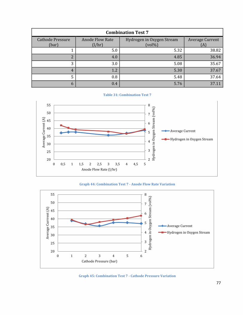
77

Combination Test 7




Average Current (A)

1 5.0 5.32 38.82

2 4.0 4.85 36.94

3 3.0 5.08 35.67

4 1.2 5.30 37.67

5 0.8 5.48 37.64

6 0.4 5.76 37.11




2

3

4

5

6

7

8

20

25

30

35

40

45

50

55

0 0,5 1 1,5 2 2,5 3 3,5 4 4,5 5

Hy

dro

gen

in O

xyge

n S

trea

m (

vo

l%)

Av

erag

e C

urr

ent

(A)


Average Current


2

3

4

5

6

7

8

20

25

30

35

40

45

50

55

0 1 2 3 4 5 6

Hy

dro

gen

in O

xyge

n S

trea

m (

vo

l%)

Av

erag

e C

urr

ren

t (A

)


Average Current


78

Combination Test 8



Hydrogen in Oxygen Stream %

Average Current (A)

1 5.0 4.08 38.05

2 4.0 3.95 38.18

3 3.0 3.98 38.70

4 1.2 3.81 40.64

5 0.8 3.66 40.59

6 0.4 3.65 40.26




2

3

4

5

6

7

8

20

25

30

35

40

45

50

55

0 0,5 1 1,5 2 2,5 3 3,5 4 4,5 5

Hy

dro

gen

in O

xyge

n S

trea

m (

vo

l%)

Av

erag

e C

urr

ent

(A)


Average Current


2

3

4

5

6

7

8

20

25

30

35

40

45

50

55

0 1 2 3 4 5 6

Hy

dro

gen

in O

xyge

n S

trea

m (

vo

l%)

Av

erag

e C

urr

ent

(A)


Average Current


79

14 REFERENCES

Awasthi A Scott K, Basu S Dynamic modeling and simulation of a proton exchange membrane

electrolyzer for hydrogen production [Journal] // International Journal for Hydrogen Energy, vol.36,

pp. 14779-14786. - 2011.

Barbir F Fuel Cells: Theory and practice [Book]. - Amsterdam : Elsevier Academic Press, 2013.

Bensmann B, Hanke-Rauschenbach R and Sundmacher K In-situ measurement of hydrogen

crossover in polymer electrolyte membrane water electrolysis, vol. 39, pp. 49-53 [Journal] //

International Journal for Hydrogen Energy. - 2014.

Bertuccioli L Chan A, Hart D, Lehner F, Madden B , Standen E Study on development of water

electrolysis in the EU [Journal] // Fuel Cells and Hydrogen Joint Undertaking. - 2014.

Carmo M Fritz D, Mergel J, Stolten D Comprehensive Review on PEM water electrolysis

[Journal] // International Journal of Hydrogen Energy, volume 38, pp. 4901-4934. - 2013.

Choi A simple model for solid polymer electrolyte (SPE) water electrolysis [Journal] // Solid State

Ionics,vol. 175, pp. 535-539. - 2004.

Decourt B Lajoie B, Debarre, R Soupa The hydrogen-based energy conversion [Report]. - [s.l.] :

FactBook The SBC Energy Institute., 2014.

Faulkner Bard and Electrochemical methods: fundamentals and applications [Book]. - New York :

John Wiley & Sons, 1980.

Friere Gonzalez Effect of membrane characteristics and humidification conditions on the

impedance response of polymer electrolyte fuel cells [Journal] // Journal of Electroanalytical

Chemistry, vol. 503, no. 1-2, pp. 57–68. - 2001.

Gandia Arzamendi , Dieguez Renewable Hydrogen Technolgies [Journal] // Elsevier. - 2013.

García-Valverde R Espinosa N, Urbina A Simple PEM water electrolyser model and experimental

validation [Journal] // International Journal of Hydrogen Energy, vol. 37, no. 2, pp. 1927–1938. -

2012.

Hydrogenics [Online] // www.hydrogenics.com. - 2015.

Ito H [et al.] Properties of Nafion under PEM water electrolysis conditions, vol. 36, pp. 10527-

10540 [Journal] // International Journal for Hydrogen Energy. - 2011.

Lee B, Park K and Kim HM Dynamic simulation of PEM water electrolysis and comparison with

experiments [Journal] // International Journal of Electrochemical Sciences, pp. 235-248. - 2013.

Lee W-J. and Lee Y-K Internal Gas Pressure Charateristics Generated during Coal Carbonization in a

Coke Oven [Journal] // Energy & Fuels. - 2001.

80

Lehner M Tichle R, SteinmüllerH, Koppe M Power-to-gas: technology and business models

[Book]. - New York : Springer International Publishing, 2014.

Marangio F Santarelli M, Calì M Theoretical model and experimental analysis of a high pressure

PEM water electrolyser for hydrogen production [Journal] // International Journal of Hydrogen

Energy, vol. 34, no. 3, pp. 1143–115. - 2009.

McAuliffe Hydrogen and energy [Book]. - London : Macmillan Press Ltd, 1980.

Medici EF and Allen JS Scaling percolation in thin porous layers [Journal] // Physics of Fluids AIP,

vol. 23. - 2011.

Medici EF and Allen JS The effects of morphological and wetting properties of porous transport

layers on water movement in PEM fuel cells [Journal] // Journal of Electrochemical Society, vol. 157,

pp. 1505-1515. - 2010.

Medina P and Santarelli M Analysis of water transport in a high pressure PEM electrolyzer, vol. 35,

pp. 5173-5186 [Journal] // International Journal for Hydrogen Energy. - 2010.

Meier F and Eingenberger G Transport parameters for the modelling of water transport in

ionomer membrane for PEM fuel cells [Journal] // Electrochemical Acta, vol. 49, pp. 1731-1742. -

2004.

Melis Green alga hydrogen production: progress, challenges and prospects [Journal] //

International Journal of Hydrogen Energy. - 2002.

Ni [et al.] A review and recent developments in photocatalytic water-splitting using TiO2 for

hydrogen production [Journal] // Renewable and Sustainable Energy Reviews. - 2007.

Nieminen J Dincer I,Naterer G Comparative performance analysis of PEM and solid oxide steam

electrolysers [Journal] // International Journal of Hydrogen Energy, vol. 35, no. 20, pp. 10842–

1085. - 2010.

Otero J Sese J, Michaus I, Santa Maria M, Guelbenzu E, Irustu S, Carrilero I, Arruebo M

Sulphonated polyether ether ketone diaphragms used in commercial scale alkaline water

electrolysis [Journal] // Journal of Power Sources,vol. 247, pp. 967–997. - 2014.

Rahim Abdol AH [et al.] An overview of polymer electrolyte membrane electrolyzer for hydrogen

production: Modeling and mass transport [Journal] // Journal of Power Sources, vol. 309, pp.56-

65. - 2016.

Sarat S Sammes N, Smirnova A Bismuth oxide doped scandia-stabilized zirconia electrolyte for the

intermediate temperature solid oxide fuel cells [Journal] // Journal of Power Sources, vol. 160, no. 2,

pp. 892–896. - 2006.

Schalenbach M [et al.] Pressurized PEM water electrolysis: efficiency and gas crossover

[Journal] // International Journal for Hydrogen Energy, vol. 38, pp. 14921-14933. - 2013.

81

Smolinka Tom Water Electrolysis: Status and Potential for Development [Report]. - [s.l.] :

Fraunhofer ISE, 2014.

Staser J and Ramasamy RP Effect of Water on the Electrochemical Oxidation of Gas-Phase SO2 in

PEM Electrolyzer for H2 production [Journal] // The Electrochemical Society, vol. 11. - 2007.

Suermann M, Schmidt TJ and Büchi FN Investigation of Mass Transport Losses in Polymer

Electrolyte Electrolysis Cells [Journal] // The Electrochemical Society. - 2015.

Sun Shucheng, Xiao Yu and Liang Dong Behaviors of a proton exchange membrane electrolyzer

under water starvation, RSC vol.5 , pp. 14506 [Journal] // Royal Society of Chemistry. - 2015.

Tao Y. Chen Y., Wu Y., Hi Y, Zhou Z. High hydrogen yield from a two-step process of dark- and

photo-fermentation of sucrose [Journal] // International Journal of Hydrogen Energy. - 2007.

Tilak B Lu P, Colman J, Srinivasan Comprehensive treatise of electrochemistry, volume 2:

Electrochemical processing [Book]. - New York : Plenum Press, 1981.

Trinke P, Bensmann B and Hanke-Rauschenbach R Current density effect on hydrogen

permeation in PEM water electrolyzers, vol.42, pp. 14355-14366 [Journal] // International Journal

of Hydrogen Energy. - 2017.

Ulleberg Modeling of advanced alkaline electrolyzers: a system simulation approach [Journal] //

International Journal of Hydrogen Energy, vol. 28, no. 1, pp. 21–33. - 2003.

Ursúa A Gandia L, Sanchis Hydrogen production from water electrolysis: current status and future

trends [Journal] // Proceedings of the IEEE, vol. 100, no. 2, pp. 410–426.. - 2012.

Vladimir A. Blagojević Dejan G. Minić Hydrogen Economy: Modern Concepts, Challenges and

Perspectives [Book]. - [s.l.] : Intech, 2012.

Wagner N and Gülzow E Change of electrochemical impedance spectra (EIS) with time during CO-

poisoning of the Pt-anode in a membrane fuel cell, vol. 127, no. 1-2, pp. 341–347 [Journal] // Journal

of Power Sources. - 2004.

Wargo EA Hanna AC, Cecan A, Kalidindi SR, Kumbur SC Selection of representative volume

elements for pore-scale analysis of transport in fuel cell materials [Journal] // Journal of Power

Sources, vol. 197, pp. 168-179. - 2012.

Zawodzinski TA, Thomas ES and Jestel R A comparative study of water uptake by and transport

through ionomeric fuel cell membranes, vol. 140, pp. 1981-1985 [Journal] // Journal of

Electrochemica Society. - 1993.

master thesis - dlr portalelib.dlr.de/114051/1/master thesis report_sangram.pdfmaster thesis...

Documents