MAT 2009: Operations Research and Optimization

2010/2011

John F. Rayman

Department of MathematicsUniversity of Surrey

Introduction

The assessment for the this module is based on a class test counting for 10% and an as-sessed coursework for 15% of total module marks and an examination which counts for theremaining 75%.

Contacting the lecturer

My office is 16AA04, my internal telephone extension 2637. If I am not in my office pleasefeel free to e-mail me on j.rayman@surrey.ac.uk to make an appointment. My website ishttp://personal.maths.surrey.ac.uk/st/J.Rayman.

Notes

These notes were originally produced by Dr. David Fisher. They are issued with numerousgaps which will be completed during lectures. Supplementary material will also be dis-tributed from time to time.

Lecture attendance is therefore essential to gain a full understanding of thematerial.

Exercises

There are exercises at the end of each chapter which will be dealt with in tutorial sessionsand solutions will be distributed progressively.

Background material

While these notes contain all the material you will need to cover during the module there arenumerous excellent textbooks in the library. Although they contain far more material thanwill be covered during the module they provide interesting and useful background and youare encouraged to look at the early chapters of some of them. Here are some suggestions:

• Introduction to Operations Research, by F Hillier and G Lieberman (McGraw-Hill)

• Operations Research: An Introduction, by H A Taha (Prentice Hall)

• Operations Research: Applications and Algorithms, by Wayne L Winston (Thomson)

1

• Operations Research: Principles and Practice, by Ravindran, Phillips and Solberg(Wiley)

• Schaum’s Outline of Operations Research, by R Bronson (McGraw-Hill)

• Linear and Non-linear Programming by S Nash and A Sofer (McGraw Hill)

2

Chapter 1

Linear Programming

1.1 Introduction

Mathematical models in business and economics often involve optimization, i.e. findingthe optimal (best) value that a function can take. This objective function might representprofit (to be maximized) or expenditure (to be minimized). There may also be constraintssuch as limits on the amount of money, land and labour that are available.

Operations Research (OR), otherwise known as Operational Research or Management Sci-ence, can be traced back to the early twentieth century. The most notable developments inthis field took place during World War II when scientists were recruited by the military tohelp allocate scarce resources. After the war there was a great deal of interest in applyingOR methods in business and industry, and the subject expanded greatly during this period.

Many of the techniques that we shall study in the first part of the course were developed atthat time. The Simplex algorithm for Linear Programming, which is the principal techniquefor solving many OR problems, was formulated by George Dantzig in 1947. This methodhas been applied to problems in a wide variety of disciplines including finance, productionplanning, timetabling and aircraft scheduling. Nowadays, computers can solve large scaleOR problems of enormous complexity.

Later in the course we consider optimization of non-linear functions. The methods hereare based on calculus. Non-linear problems with equality constraints will be solved usingthe method of Lagrange multipliers, named after Joseph Louis Lagrange (1736 - 1812). Asimilar method for inequality constraints was developed by Karush in 1939 and by Kuhnand Tucker in 1951.

3

1.2 The graphical method

In a Linear Programming (LP) problem, we seek to optimize an objective functionwhich is a linear combination of some decision variables x1, . . . , xn. These variables arerestricted by a set of constraints, expressed as linear equations or inequalities.

When there are just two decision variables x1 and x2, the constraints can be illustratedgraphically in a plane. We represent x1 on the horizontal axis and x2 on the vertical axis.

To find the region defined by ax1 + bx2 ≤ c, first draw the straight line with equationax1 + bx2 = c. Assuming a 6= 0 and b 6= 0, this line crosses the axes at x1 =

c

aand x2 =

c

b.

If b > 0, then ax1 + bx2 ≤ c defines the region on and below the line and ax1 + bx2 ≥ cdefines the region on and above the line. If b < 0 then this situation is reversed. It is usualto shade along the side of the line away from the region that is being defined.

A strict inequality (< or > rather than ≤ or ≥) defines the same region, but the line itselfis not included. This can be shown by a dotted line.

x1 < c to the left of the vertical line x1 = c, and x1 > c to the right of this line.

x2 < c below the horizontal line x2 = c, and x2 > c above this line.

A simple way of deciding which side of a line satisfies a given inequality is to consider theorigin (0, 0). For example, 2x1 − 3x2 ≤ 5 defines that side of the line 2x1 − 3x2 = 5 whichcontains the origin, since 2(0) − 3(0) ≤ 5.

If the origin lies on the line, consider a convenient point which is not on the line, e.g. (1, 1).

For a general LP problem, a set of values of the decision variables can be represented as avector (x1, . . . , xn) ∈ Rn. We make the following definitions:

• A vector which satisfies all the constraints is called a feasible point.

• The set of all feasible points is called the feasible region or solution space for theproblem.

• Points where at least one constraint fails to hold are called infeasible points. Thesepoints lie outside the feasible region.

• The optimum or optimal value of the objective function is the maximum or mini-mum value, whichever the problem requires.

• A feasible point at which the optimal value occurs is called an optimal point, andgives an optimal solution.

Example 1: Containers problem

To produce two types of container, A and B, a company uses two machines, M1 and M2.Producing one of container A uses M1 for 2 minutes and M2 for 4 minutes. Producing one ofcontainer B uses M1 for 8 minutes and M2 for 4 minutes. The profit made on each containeris £30 for type A and £45 for type B. Determine the production plan that maximizes thetotal profit per hour.

4

• Identify the decision variables.

• Formulate the objective function and state whether it is to be maximized or minimized.

• List the constraints. The allowable values of the decision variables are restricted by:

The following diagram shows the feasible region for the problem.

x1

x2

0 5 10 15 20 25 30

0

5

10

15

There are infinitely many feasible solutions. An optimal one can be found by consideringthe slope, and direction of increase, of the objective function z = 30x1 + 45x2.

Different values of the objective function correspond to straight lines with equations of the

form 30x1 +45x2 = c for varying values of c. These lines are all parallel, with gradient −23.

Draw such a line, e.g. 2x1 + 3x2 = 6 which crosses the axes at (3, 0) and (0, 2). To findthe maximum profit we translate this ‘profit line’ in the direction of increasing z, keepingits slope the same, until moving it any further would take it completely outside the feasibleregion.

We see that the optimum occurs at a corner point (or extreme point) of the feasibleregion, at the intersection of the lines that correspond to the two machine constraints.Hence the optimal values of x1 and x2 are the solutions of the simultaneous equations

2x1 + 8x2 = 60 and 4x1 + 4x2 = 60,

i.e. (x1, x2) = (10, 5). The optimal value of the objective function is then z = 525.

Thus the optimal production plan is to produce 10 type A containers and 5 type B con-tainers per hour. This plan yields the maximum profit, which is £525 per hour.

5

We shall show later that if a LP problem has an optimal solution then there is an extremepoint of the feasible region where this solution occurs.

There can sometimes be optimal solutions which do not occur at extreme points. If twovertices P and Q of the feasible region give equal optimal values for the objective functionthen the same optimal value occurs at all points on the line segment PQ.

Suppose the profit on container A is changed to £p. If454

< p < 45 then the optimal

solution still occurs at (10, 5). If p =454

or p = 45 there are multiple optimal points, all

yielding the same profit. If p > 45 then (15, 0) is optimal. If p <454

then (0, 7.5) is optimal,but 7.5 containers cannot be made. The best integer solution can be found by inspection.

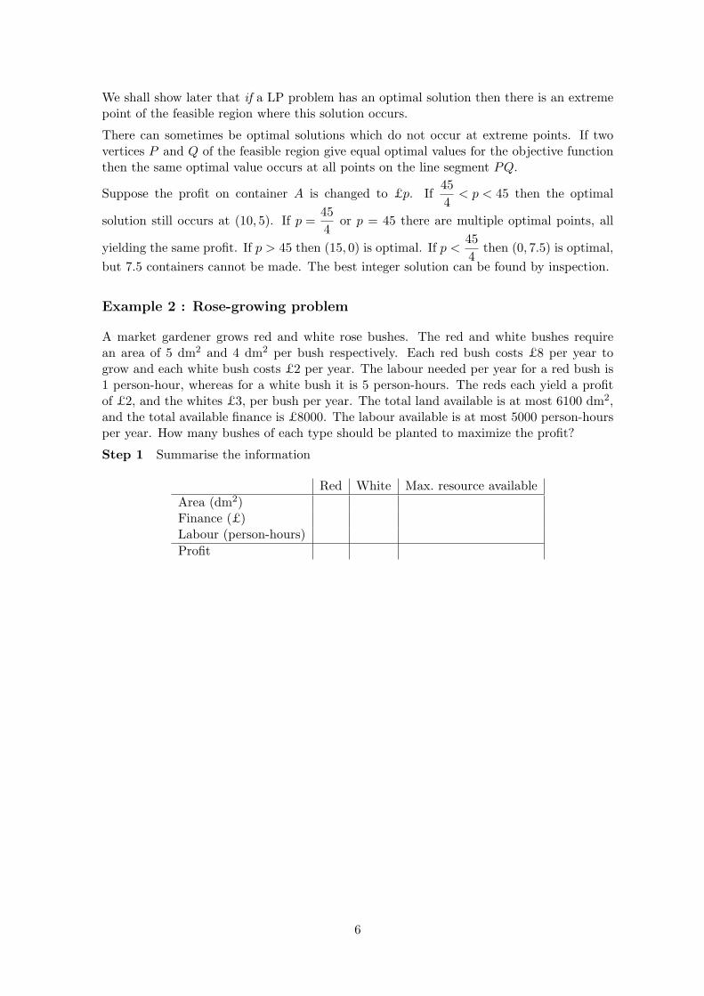
Example 2 : Rose-growing problem

A market gardener grows red and white rose bushes. The red and white bushes requirean area of 5 dm2 and 4 dm2 per bush respectively. Each red bush costs £8 per year togrow and each white bush costs £2 per year. The labour needed per year for a red bush is1 person-hour, whereas for a white bush it is 5 person-hours. The reds each yield a profitof £2, and the whites £3, per bush per year. The total land available is at most 6100 dm2,and the total available finance is £8000. The labour available is at most 5000 person-hoursper year. How many bushes of each type should be planted to maximize the profit?

Step 1 Summarise the information

Red White Max. resource availableArea (dm2)Finance (£)Labour (person-hours)Profit

6

Step 2 Define the decision variables.

Step 3 Specify the objective function.

Step 4 Identify the constraints and the non-negativity conditions.

Step 5 Sketch the feasible region.

Step 6 Method 1 Sketch a line of the form z = constant and translate this line, in thedirection in which z increases, until it no longer intersects the feasible region.

Method 2 Evaluate z at each of the extreme points and see where it is greatest.

7

Final answer:

Note that the original problem was stated in words: it did not mention the variables x1

and x2 or the objective function z. Your final answer should not use these symbols, as theyhave been introduced to formulate the mathematical model.

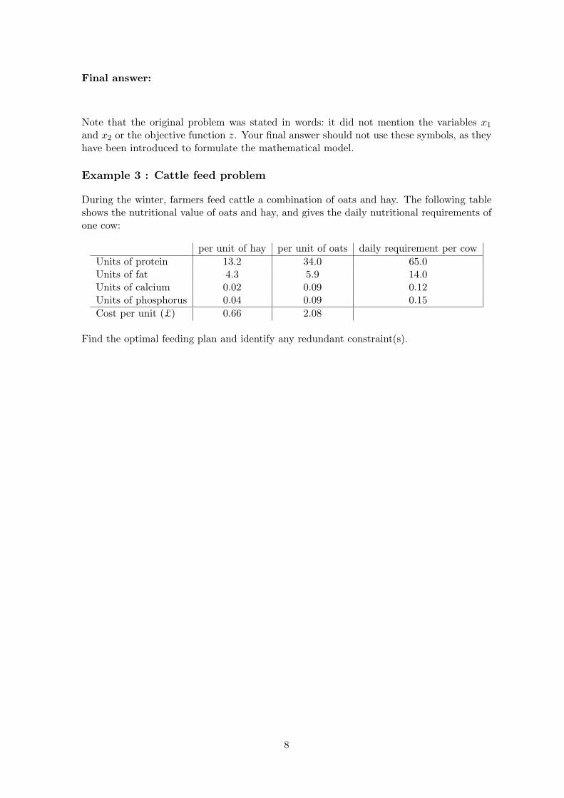
Example 3 : Cattle feed problem

During the winter, farmers feed cattle a combination of oats and hay. The following tableshows the nutritional value of oats and hay, and gives the daily nutritional requirements ofone cow:

per unit of hay per unit of oats daily requirement per cowUnits of protein 13.2 34.0 65.0Units of fat 4.3 5.9 14.0Units of calcium 0.02 0.09 0.12Units of phosphorus 0.04 0.09 0.15Cost per unit (£) 0.66 2.08

Find the optimal feeding plan and identify any redundant constraint(s).

8

Decision variables

Objective function

Constraints and non-negativity conditions

Draw the feasible region

0

0.5

1

1.5

2

2.5

x2

1 2 3 4 5 6

x1

Extreme points (calculated to two decimal places where appropriate)

9

Final Answer

1.3 Convexity and extreme points

Definitions

The feasible region for a LP problem is a subset of the Euclidean vector space Rn, whoseelements we call points. The norm of x = (x1, . . . , xn) is |x| =

√x1

2 + · · · + xn2.

An equation of the form a1x1 + · · · + anxn = b, or atx = b, defines a hyperplane in Rn.A hyperplane in R2 is a straight line. A hyperplane in R3 is a plane.

Any hyperplane determines the half-spaces given by atx ≤ b and atx ≥ b.

A convex linear combination of x and y is an expression of the form (1−r)x+ry where0 ≤ r ≤ 1. In R2 and R3, such a weighted average of x and y represents a point on thestraight line segment between x and y.

More generally, a convex linear combination of the points x1, . . . , xm is an expressionof the form r1x1 + · · · + rmxm, where r1 + · · · + rm = 1 and ri ≥ 0 for i = 1, . . . , m.

A convex set in Rn is a set S such that if x,y ∈ S then (1− r)x+ ry ∈ S for all r ∈ [0, 1].It follows that a convex linear combination of any number of elements of S is also in S.

A convex set can be interpreted in R2 and R3 as a region S such that if A and B are anytwo points in S, every point on the straight line segment AB lies in S.

Examples of convex sets include: Rn itself; any vector subspace of Rn; any interval of thereal line; any hyperplane; any half-space; the interior of a circle or sphere.

We can often use a graph to decide whether a subset of R2 is convex, e.g. {(x, y) : y ≥ x2}is convex whereas {(x, y) : y ≤ x3} is not convex.

If S1, . . . , Sn are convex sets, their intersection S1 ∩ · · · ∩ Sn is also convex.

An extreme point, corner point or vertex of a convex set S is a point z ∈ S such thatthere are no two distinct points x,y ∈ S with z = (1 − r)x + ry for some r ∈ (0, 1).

A neighbourhood of a point x ∈ Rn is a set of the form {y ∈ Rn : |y− x| < ε} for someε > 0. This can also be called an ε-neighbourhood or an open ball of radius ε.

Let S be a subset of Rn. A point x in S is an interior point of S if some neighbourhoodof x is contained in S. S is an open set if every point of S is an interior point.

A point y, not necessarily in S, is a boundary point of S if every neighbourhood of ycontains a point in S and a point not in S. The set of all boundary points of S is calledthe boundary of S. S is a closed set if every boundary point of S is in S.

Every point in S is either an interior point or a boundary point of S.

Some sets are neither open nor closed. Others, such as Rn itself, are both open and closed.

A set S ⊂ Rn is bounded if there exists a real number M such that |x| < M for all x ∈ S.

S is a compact set if it is both closed and bounded.

10

If S is not bounded it has a direction of unboundedness, i.e. a vector u such that forall x ∈ S and k ≥ 0, x + ku ∈ S. (In general there are infinitely many such directions.)

The feasible region for a LP problem with n decision variables is the intersection of a finitenumber of half-spaces in Rn. Hence it is convex. The region is closed, since it includes thehyperplanes which form its boundary, and it has a finite number of extreme points.

Proposition 1.1 (Weierstrass’s Theorem, or the Extreme Value Theorem)Let f be a continuous real-valued function defined on a non-empty compact subset S of Rn.Then f(x) attains minimum and maximum values on S, i.e. there exist xm,xM ∈ S suchthat −∞ < f(xm) ≤ f(x) ≤ f(xM ) < ∞ for all x ∈ S.

Example Consider the problem: Maximize z = 4x1 + x2 + 3x3 , subject to

x1 + x2 ≤ 6, − x2 + 2x3 ≤ 4, 0 ≤ x1 ≤ 4, 0 ≤ x2 ≤ 4, x3 ≥ 0.

The feasible set is a convex polyhedron or simplex with seven plane faces, as shown. As itis closed and bounded, and any linear function is continuous, Weierstrass’s theorem tells usthat z attains a greatest and least value over this region. Clearly the minimum occurs at(0, 0, 0). It turns out that z is maximum at (4, 2, 3).

Considering other objective functions with the same feasible region, x1+x2+x3 is maximumat (2, 4, 4), while x1 − 3x2 − x3 is maximum at (4, 0, 0).

Proposition 1.2 Let S be the intersection of a finite number of half-planes in Rn. Letv1, . . . ,vm be the extreme points of S.

Then x ∈ S if and only if x = r1v1 + · · ·+ rmvm + u where r1 + · · ·+ rm = 1, each ri ≥ 0,u = 0 if S is bounded and u is a direction of unboundedness otherwise.

The proof of the ‘if’ part of the above result is in the Exercises. The ‘only if’ part is moredifficult to prove, but by assuming it we can show the following:

Proposition 1.3 (The Extreme Point Theorem) Let S be the feasible region for a lin-ear programming problem.

1. If S is non-empty and bounded then an optimal solution of the problem exists, andthere is an extreme point of S at which it occurs.

11

2. If S is non-empty and not bounded then if an optimal solution to the problem exists,there is an extreme point of S at which it occurs.

Proof

Let the objective function be z = c1x1 + · · · + cnxn = ctx.S is closed so in case 1 it is compact, hence by Proposition 1.1 z attains its maximum andminimum values at some points in S. In case 2 we are assuming that the required optimumis attained.

Assume z is to be maximized, and takes its maximum value over S at x∗ ∈ S. (If z is tobe minimized, apply the following reasoning to −z.)

Let v1, . . . ,vm be the extreme points of S.

By Proposition 1.2, x∗ = r1v1 + · · · + rmvm + u where r1 + · · · + rm = 1, each ri ≥ 0, andu is 0 in case 1 or a direction of unboundedness in case 2.

Suppose, for a contradiction, that there is no extreme point of S at which z is maximum,so ctvi < ctx∗ for i = 1, . . . ,m.

Then ctx∗ = ct(r1v1 + · · · + rmvm + u)

= r1ctv1 + · · · + rmctvm + ctu

< r1ctx∗+· · ·+rmctx∗+ctu (since ctvi < ctx∗ and ri ≥ 0 for i = 1, . . . , m)

= (r1 + · · · + rm)ctx∗ + ctu

= ctx∗ + ctu (since r1 + · · · + rm = 1)

= ct(x∗ + u).

But x∗ + u ∈ S and ctx is maximized over S at x∗, so ctx∗ ≥ ct(x∗ + u).

We have a contradiction, so z must take its maximum value at some extreme point of S. �

12

Exercises 1

1. Solve the following Linear Programming problems graphically.

(a) Maximize z = 2x1 + 3x2 subject to2x1 + 5x2 ≤ 10, x1 − 4x2 ≥ −1, x1 ≥ 0, x2 ≥ 0.

(b) Minimize z = 4x2 − 5x1 subject tox1 + x2 ≤ 10, −2x1 + 3x2 ≥ −6, 6x1 − 4x2 ≤ 13.

2. The objective function z = px + qy, where p > 0, q > 0, is to be maximized subjectto the constraints 3x + 2y ≤ 6, x ≥ 0, y ≥ 0.

Find the maximum value of z in terms of p and q. (There are different cases, dependingon the relative sizes of p and q.)

3. A company makes two products, A and B, using two components X and Y .

To produce 1 unit of A requires 5 units of X and 2 units of Y .To produce 1 unit of B requires 6 units of X and 3 units of Y .

At most 85 units of X and 40 units of Y are available per day.

The company makes a profit of £12 on each unit of A and £15 on each unit of B.

Assuming that all the units produced can be sold, find the number of units of eachproduct that should be made per day to optimze the profit.

If the profit on B is fixed, how low or high would the profit on A have to becomebefore the optimal production schedule changed?

4. A brick company manufactures three types of brick in each of its two kilns. Kiln Acan produce 2000 standard, 1000 oversize and 500 glazed bricks per day, whereas kilnB can produce 1000 standard, 1500 oversize and 2500 glazed bricks per day. The dailyoperating cost for kiln A is £400 and for kiln B is £320.

The brickyard receives an order for 10000 standard, 9000 oversize and 7500 glazedbricks. Determine the production schedule (i.e. the number of days for which eachkiln should be operated) which will meet the demand at minimum cost (assuming bothkilns can be operated immediately) in each of the following separate cases. (Note: thekilns may be used for fractions of a day.)

(a) there is no time limit,

(b) kiln A must be used for at least 5 days,

(c) there are at most 2 days available on kiln A and 9 days on kiln B.

5. A factory can assemble mobile phones and laptop computers. The maximum amountof the workforce’s time that can be spent on this work is 10 hours per day. Before thephones and laptops can be assembled, the component parts must be purchased. Themaximum value of the stock that can be held for a day’s assembly work is £2200.

In the factory, a mobile phone takes 10 minutes to assemble using £10 worth ofcomponents whereas a laptop takes 1 hour 40 minutes to assemble using £500 worthof components.

The profit made on a mobile phone is £5 and the profit on a laptop is £100.

(a) Summarise the above information in a table.

13

(b) Assuming that the factory can sell all the phones and laptops that it assembles,formulate the above information into a Linear Programming problem.

(c) Determine the number of mobile phones and the number of laptops that shouldbe made in a day to maximise profit.

(d) The market for mobile phones is saturating. In response, retailers are droppingprices which means reduced profits. How low can the profit on a mobile phonego before the factory should switch to assembling only laptops?

6. In the Containers problem (Example 1), suppose we write the machine constraints as2x1 + 8x2 + x3 = 60 and 4x1 + 4x2 + x4 = 60, where x3 and x4 are the number ofminutes in an hour for which M1 and M2 are not used, so x3 ≥ 0 and x4 ≥ 0.

Show that the objective function can be written as

z = 30(

10 +16x3 −

13x4

)+ 45

(5 − 1

6x3 +

112

x4

).

By simplifying this, deduce that that the maximum value of z occurs when x3 = x4 = 0and state this maximum value.

7. By sketching graphs and using the fact that the straight line joining any two pointsof a convex set lies in the set, decide which of the following subsets of R2 are convex.

(a) {(x, y) : xy ≤ 1, x ≥ 0, y ≥ 0}, (b) {(x, y) : xy ≤ −1, x ≥ 0},(c) {(x, y) : y − x2 ≤ 1}, (d) {(x, y) : 2x2 + 3y2 < 6},(e) {(x, y) : x2 − y2 = 1}, (f) {(x, y) : y ≤ lnx, x > 0}.

8. Let a = (a1, . . . , an) be a fixed element of Rn and let b be a real constant. Let x1 andx2 lie in the half-space atx ≤ b, so that atx1 ≤ b and atx2 ≤ b. Show that for allr ∈ [0, 1], at((1 − r)x1 + rx2) ≤ b. Deduce that the half-space is a convex set.

9. Let S and T be convex sets. Show that their intersection S ∩ T is a convex set.

(Hint : let x,y ∈ S ∩ T , so x,y ∈ S and x,y ∈ T . Why must (1 − r)x + ry be inS ∩ T for 0 ≤ r ≤ 1?)

Generalise this to show that if S1, . . . , Sn are convex sets then S = S1 ∩ · · · ∩ Sn isconvex. Deduce that the feasible region for a linear programming problem is convex.

10. Let S be the feasible region for a Linear Programming problem. If an optimal solutionto the problem does not exist, what can be deduced about S from Proposition 1.3?

11. Prove that every extreme point of a convex set S is a boundary point of S. (Method:suppose x is in S and is not a boundary point. Then some neighbourhood of x mustbe contained in S (why?) Deduce that x is a convex linear combination of two pointsin this neighbourhood and so x is not an extreme point.)

12. Prove the ‘if’ part of Proposition 1.2 as follows. Let the half-planes defining S bea1

tx ≤ b1, . . . ,aktx ≤ bk. As vi ∈ S, all these inequalities hold when x = vi for

i = 1, . . . ,m.

Show that x = r1v1+· · ·+rmvm also satisfies all the inequalities, where r1+· · ·+rm =1 and each ri ≥ 0.

Deduce further that if S is unbounded and u is a direction of unboundedness thenr1v1 + · · · + rmvm + u ∈ S.

14

Chapter 2

The Simplex Method

2.1 Matrix formulation of Linear Programming problems

If a linear programming problem has more than two decision variables then a graphical so-lution is not possible. We therefore develop an algebraic, rather than geometric, approach.

Definitions

x is a non-negative vector, written x ≥ 0, if every entry of x is positive or zero.

The set of non-negative vectors in Rn is denoted by Rn+.

u ≥ v means that every entry of the vector u is greater than or equal to the correspondingentry of v. Thus u ≥ v, or v ≤ u, is equivalent to u − v ≥ 0.

Let x and y be non-negative vectors. Then it is easy to show that:

(i) x + y = 0 ⇒ x = y = 0, (ii) xty ≥ 0, (iii) u ≥ v ⇒ xtu ≥ xtv.

Recall that for matrices A and B, (AB)t = BtAt.

For vectors x and y, we have xty = ytx and xtAy = ytAtx (these are all scalars).

We shall sometimes need to work with partitioned matrices. Recall that if two matricescan be split into blocks which are conformable for matrix multiplication, then(

A11 A12

A21 A22

)(B11 B12

B21 B22

)=(

A11B11 + A12B21 A11B12 + A12B22

A21B11 + A22B21 A21B12 + A22B22

).

Now consider a typical Linear Programming problem. We seek values of the decision vari-ables x1, x2, . . . , xn which optimize the objective function

z = c1x1 + c2x2 + · · · + cnxn

subject to the constraintsa11x1 + a12x2 + · · · + a1nxn ≤ b1

a21x1 + a22x2 + · · · + a2nxn ≤ b2...

am1x1 + am2x2 + · · · + amnxn ≤ bm

and the non-negativity restrictions x1 ≥ 0, x2 ≥ 0, . . . , xn ≥ 0.

15

A maximization LP problem can be written in matrix-vector form as

Maximize z = ctxsubject to Ax ≤ b (LP1)and x ≥ 0

where A is the m × n matrix with (i, j) entry aij and

x =

x1...

xn

, b =

b1...

bm

, c =

c1...

cn

.

The problem (LP1) is said to be feasible if the constraints are consistent, i.e. if there existsx ∈ Rn

+ such that Ax ≤ b. Any such vector x is a feasible solution of (LP1). If a feasiblepoint x maximizes z subject to the constraints, x is an optimal solution.

The problem is unbounded if there is no finite maximum over the feasible region, i.e. thereis a sequence of vectors {xk} satisfying the constraints, such that ctxk → ∞ as k → ∞.

The standard form of a LP problem is defined as follows:

• The objective function is to be maximized.

• All constraints are equations with non-negative right-hand sides.

• All the variables are non-negative.

Any LP problem can be converted into standard form by the following methods:

Minimizing f(x) is equivalent to maximizing −f(x). Thus the problem

Minimize c1x1 + c2x2 + · · · + cnxn

is equivalent to

Maximize − c1x1 − c2x2 − · · · − cnxn

subject to the same constraints, and the optimum occurs at the same values of x1, . . . , xn.

Any equation with a negative right hand side can be multiplied through by −1 so that theright-hand side becomes positive. Remember that if an inequality is multiplied through bya negative number, the inequality sign must be reversed.

A constraint of the form ≤ can be converted to an equation by adding a non-negative slackvariable on the left-hand side of the constraint.

A constraint of the form ≥ can be converted to an equation by subtracting a non-negativesurplus variable on the left-hand side of the constraint.

2.1.1 Example

Suppose we start with the problem

Minimize z = −3x1 + 4x2 − 5x3

subject to{

3x1 + 2x2 − 3x3 ≤ 42x1 − 3x2 + x3 ≤ −5

and x1 ≥ 0, x2 ≥ 0, x3 ≥ 0.

16

A variable is unrestricted if it is allowed to take both positive and negative values. Anunrestricted variable xj can be expressed in terms of two non-negative variables by substi-tuting xj = x′

j −x′′j where both x′

j and x′′j are non-negative. The substitution must be used

throughout, i.e. in all the constraints and in the objective function.

2.1.2 Example

Suppose we have to maximize z = x1 − 2x2 subject to the constraints

x1 + x2 ≤ 4, 2x1 + 3x2 ≥ 5, x1 ≥ 0 and x2 unrestricted in sign.

If a LP problem involves n main (original) variables and m inequality constraints then weneed m additional (slack or surplus) variables, so the total number of variables becomesn + m. Then the problem (LP1) can be written in the form

Maximize z = c txsubject to Ax = b (LP2)and x ≥ 0

where A is an m × (n + m) matrix, x =

x1...

xn

xn+1...

xn+m

, c =

c1...

cn

0...0

.

17

The constraints are now expressed as a linearly independent set of m equations in n + munknowns, representing m hyperplanes in Rn+m. A particular solution can be found bysetting any n variables to zero and solving for the remaining m.

A feasible solution of (LP2) is a vector v ∈ Rn+m+ such that Av = b.

Provided b ≥ 0, A = (A | Im) and then (LP2) has an obvious feasible solution x =(

0b

).

2.1.3 Example

Consider the Linear Programming problem: Maximize z = x1 + 2x2 + 3x3

subject to 2x1 + 4x2 + 3x3 ≤ 10, 3x1 + 6x2 + 5x3 ≤ 15 and x1 ≥ 0, x2 ≥ 0, x3 ≥ 0.

Introducing non-negative slack variables x4 and x5, the problem can be written as

Maximize z =(

1 2 3 0 0)

x1

x2

x3

x4

x5

subject to(

2 4 3 1 03 6 5 0 1

)x1

x2

x3

x4

x5

=(

1015

),

where x1, . . . , x5 ≥ 0.

Setting any 3 variables to zero, if the resulting equations are consistent we can solve for theother two; e.g. (1, 2, 0, 0, 0) and (0, 0, 0, 10, 15) are feasible solutions for (x1, x2, x3, x4, x5).

Note that setting x3 = x4 = x5 = 0 gives 2x1 + 4x2 = 10, 3x1 + 6x2 = 15 which are thesame equation and thus do not have a unique solution for x1 and x2.

A unique solution of (LP2) obtained by setting n variables to zero is called a basic solution.

If it is also feasible, i.e. non-negative, it is called a basic feasible solution (bfs).

The n variables set to zero are called non-basic variables. The remaining m (some ofwhich may be zero) are basic variables. The set of basic variables is called a basis.

In the above example, (0, 0, 10/3, 0,−5/3) is a basic infeasible solution. (1, 2, 0, 0, 0) is afeasible solution but not a bfs. (0, 0, 3, 1, 0) is a basic feasible solution, with basis {x3, x4}.

It can be proved that x is a basic feasible solution of (LP2) if and only if it is an extremepoint of the feasible region for (LP2) in Rn+m. The vector x consisting of the first ncomponents of x is then an extreme point of the original feasible region for (LP1) in Rn.

In any LP problem that has an optimal solution, we know by Proposition 1.3 that anoptimal solution exists at an extreme point. Hence we are looking for the basic feasiblesolution which optimizes the objective function.

Suppose we have a problem with 25 original variables and 15 constraints, giving rise to15 slack or surplus variables. In each basic feasible solution, 25 variables are set equal to

zero. There are(

4025

)possible sets of 25 variables which could be equated to zero, which

is more than 4 × 1010 combinations. Clearly an efficient method for choosing the sets ofvariables to set to zero is required! Suppose that

• we are able to find an initial basic feasible solution, say x1,

• we have a way of checking whether a given bfs is optimal, and

18

• we have a way of moving from a non-optimal bfs xi to another, xi+1, that gives abetter value of the objective function.

Combining these three steps will yield an algorithm for solving the LP problem.

If x1 is optimal, then we are done. If it is not, then we move from x1 to x2, which bydefinition is better than x1. If x2 is not optimal then we move to x3 and so on. Sincethe number of extreme points is finite and we always move towards a better one, we mustultimately find the optimal one. The Simplex method is based on this principle.

2.2 The Simplex algorithm

Consider the Linear Programming problem:

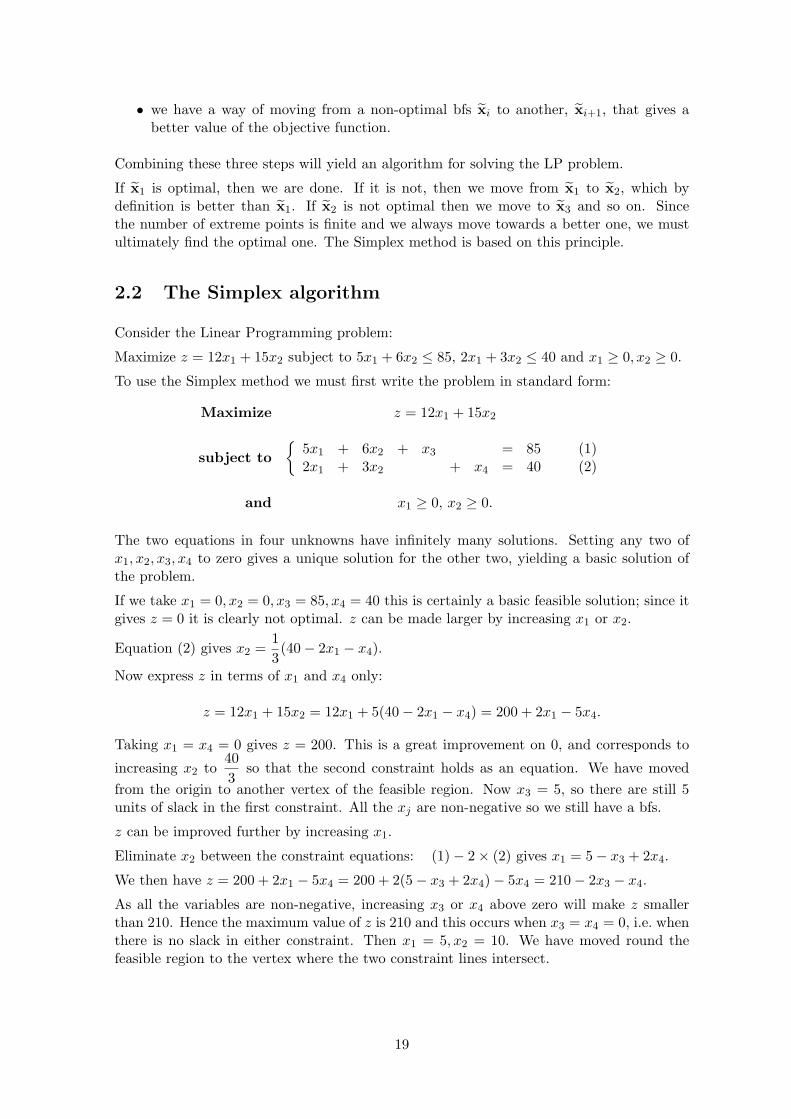
Maximize z = 12x1 + 15x2 subject to 5x1 + 6x2 ≤ 85, 2x1 + 3x2 ≤ 40 and x1 ≥ 0, x2 ≥ 0.

To use the Simplex method we must first write the problem in standard form:

Maximize z = 12x1 + 15x2

subject to{

5x1 + 6x2 + x3 = 85 (1)2x1 + 3x2 + x4 = 40 (2)

and x1 ≥ 0, x2 ≥ 0.

The two equations in four unknowns have infinitely many solutions. Setting any two ofx1, x2, x3, x4 to zero gives a unique solution for the other two, yielding a basic solution ofthe problem.

If we take x1 = 0, x2 = 0, x3 = 85, x4 = 40 this is certainly a basic feasible solution; since itgives z = 0 it is clearly not optimal. z can be made larger by increasing x1 or x2.

Equation (2) gives x2 =13(40 − 2x1 − x4).

Now express z in terms of x1 and x4 only:

z = 12x1 + 15x2 = 12x1 + 5(40 − 2x1 − x4) = 200 + 2x1 − 5x4.

Taking x1 = x4 = 0 gives z = 200. This is a great improvement on 0, and corresponds to

increasing x2 to403

so that the second constraint holds as an equation. We have movedfrom the origin to another vertex of the feasible region. Now x3 = 5, so there are still 5units of slack in the first constraint. All the xj are non-negative so we still have a bfs.

z can be improved further by increasing x1.

Eliminate x2 between the constraint equations: (1) − 2 × (2) gives x1 = 5 − x3 + 2x4.

We then have z = 200 + 2x1 − 5x4 = 200 + 2(5 − x3 + 2x4) − 5x4 = 210 − 2x3 − x4.

As all the variables are non-negative, increasing x3 or x4 above zero will make z smallerthan 210. Hence the maximum value of z is 210 and this occurs when x3 = x4 = 0, i.e. whenthere is no slack in either constraint. Then x1 = 5, x2 = 10. We have moved round thefeasible region to the vertex where the two constraint lines intersect.

19

The above working can be set out in an abbreviated way. The objective function is writtenas z − 12x1 − 15x2 = 0. This and the constraints are three equations in five unknownsx1, x2, x3, x4 and z. This system of linear equations holds at every feasible point.

We obtain an equivalent system by forming linear combinations of these equations, so longas the resulting set of equations remains linearly independent. This can be carried out mosteasily by writing the equations in the form of an augmented matrix and carrying out rowoperations, as in Gaussian elimination. This matrix is written in a way which helps us toidentify the basic variables at each stage, called a simplex tableau.

Eventually we should get an expression for the objective function in the form z = k−∑

αjxj

where each αj ≥ 0, such as z = 210 − 2x3 − x4 in the example above. Then increasing anyof the xj would decrease z, so we have arrived at a maximum value of z.

A simplex tableau consists of a grid with headings for each of the variables and a row foreach equation, including the objective function. Under the heading ‘Basic’ are the variableswhich yield a basic feasible solution when they take the values in the ‘Solution’ column andthe others are all zero. The ‘=’ sign comes immediately before the ‘Solution’ column.

You will find various forms of the tableau in different books. Some omit the z columnand/or the ‘Basic’ column. The objective function is often placed at the top. Some writersdefine the standard form to be a minimization rather than a maximization problem.

For the problem on the previous page, the initial simplex tableau is:

Basic z x1 x2 x3 x4 Solutionx3 0 5 6 1 0 85x4 0 2 3 0 1 40z 1 −12 −15 0 0 0

This tableau represents the initial basic feasible solution x1 = x2 = 0, x3 = 85, x4 = 40giving z = 0. The basic variables at this stage are x3 and x4.

The negative values in the z row show that this solution is not optimal: z−12x1−15x2 = 0so z can be made larger by increasing x1 or x2 from 0.

Increasing x2 seems likely to give the best improvement in z, as the largest coefficient in zis that of x2. We carry out row operations on the tableau so as to make x2 basic. One ofthe entries in the x2 column must become 1 and the others must become 0. The right-handsides must all remain non-negative. This is achieved by choosing the entry ‘3’ as the ‘pivot’.

Divide Row 2 by 3 to make the pivot 1. Then combine multiples of this row (only) witheach of the other rows so that all other entries in the pivot column become zero:

Basic z x1 x2 x3 x4 Solutionx3 0 1 0 1 −2 5 R1 := R1 − 2R2

x2 0 2/3 1 0 1/3 40/3 R2 := R2/3z 1 −2 0 0 5 200 R3 := R3 + 5R2

This represents the bfs z = 200 when x1 = 0, x2 =403

, x3 = 5, x4 = 0. x4 has left the basis

(it is the ‘departing variable’) and x2 has entered the basis (it is the ‘entering variable’).

Now the bottom row says z − 2x1 + 5x4 = 200 so we can still increase z by increasing x1

from 0. Thus x1 must enter the basis. The entry ‘1’ in the top left of the tableau is thenew pivot, and all other entries in its column must become 0. x3 leaves the basis.

20

Basic z x1 x2 x3 x4 Solutionx1 0 1 0 1 −2 5x2 0 0 1 −2/3 5/3 10 R2 := R2 − 2

3R1

z 1 0 0 2 1 210 R3 := R3 + 2R1

Now there are no negative numbers in the z row, which says z + 2x3 + x4 = 210.

Increasing either of the non-basic variables x3, x4 from 0 cannot increase z, so we have theoptimal value z = 210 when x3 = x4 = 0.

The tableau shows that this constrained maximum occurs when x1 = 5 and x2 = 10.

The rose-growing problem revisited

Consider the rose-growing problem from Chapter 1.

Step 1 Write the problem in standard form.

Maximise z = 2x1 + 3x2

subject to

5x1 + 4x2 + x3 = 61008x1 + 2x2 + x4 = 8000x1 + 5x2 + x5 = 5000

and xj ≥ 0 for j = 1, . . . , 5.

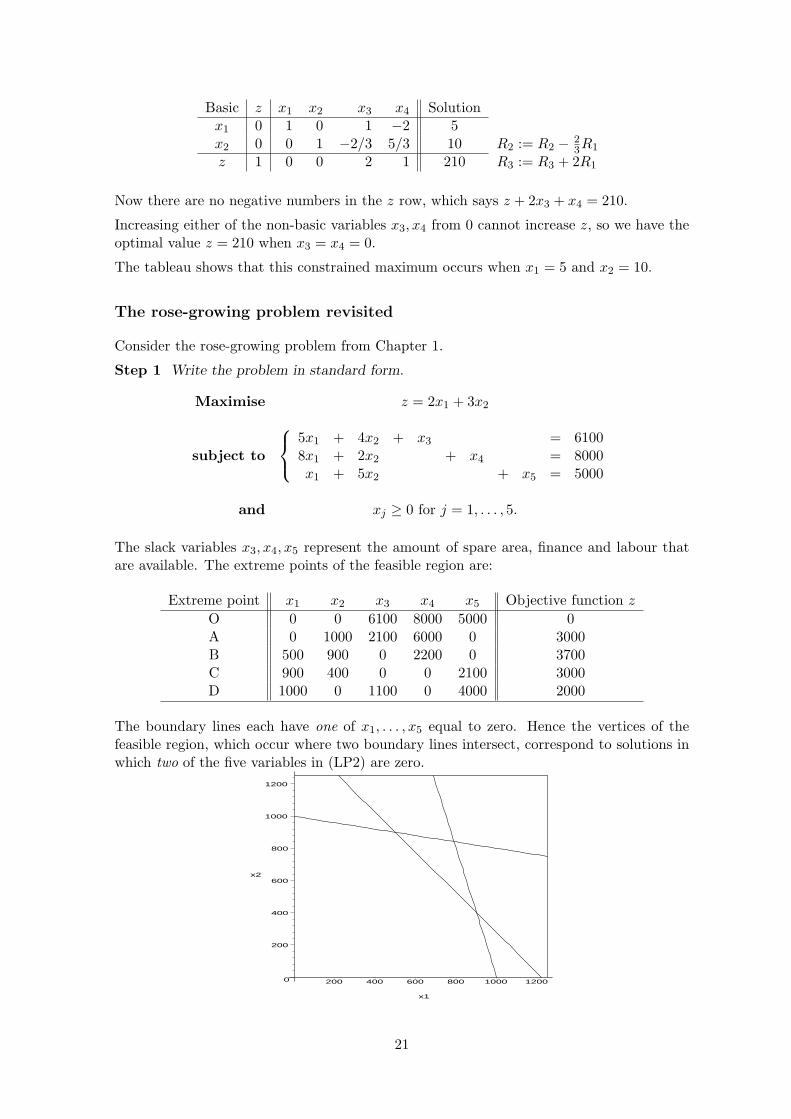
The slack variables x3, x4, x5 represent the amount of spare area, finance and labour thatare available. The extreme points of the feasible region are:

Extreme point x1 x2 x3 x4 x5 Objective function z

O 0 0 6100 8000 5000 0A 0 1000 2100 6000 0 3000B 500 900 0 2200 0 3700C 900 400 0 0 2100 3000D 1000 0 1100 0 4000 2000

The boundary lines each have one of x1, . . . , x5 equal to zero. Hence the vertices of thefeasible region, which occur where two boundary lines intersect, correspond to solutions inwhich two of the five variables in (LP2) are zero.

0

200

400

600

800

1000

1200

x2

200 400 600 800 1000 1200

x1

21

The simplex method systematically moves around the boundary of this feasible region,starting at the origin and improving the objective function at every stage.

Step 2 Form the initial tableau.

Basic z x1 x2 x3 x4 x5 Solutionx3 0 5 4 1 0 0 6100x4 0 8 2 0 1 0 8000x5 0 1 5 0 0 1 5000z 1 −2 −3 0 0 0 0

Note that the bottom row comes from writing the objective function as z − 2x1 − 3x2 = 0.

The tableau represents a set of equations which hold simultaneously at every feasible solu-tion. The ‘=’ sign in the equations occurs immediately before the solution column. Thereare 5 − 3 = 2 basic variables. Each column headed by a basic variable has an entry 1 inexactly one row and 0 in all the other rows. In the above tableau, x1 and x2 are non-basic.Setting these to zero, an initial basic feasible solution can be read directly from the tableau:x3 = 6100, x4 = 8000 and x5 = 5000, giving z = 0.

Step 3 Test for optimality: are all the coefficients in the z-row non-negative?

If so then stop, as the optimal solution has been reached. Otherwise go to Step 4.

The bottom row says z − 2x1 − 3x2 = 0, so z can be increased by increasing x1 or x2.

Step 4 Choose the variable to enter the basis: the entering variable.This will be increased from its current value of 0.

z = 2x1 + 3x2, so we should be able to increase z the most if we increase x2 from 0. (Therate of change of z is greater with respect to x2; this is called a steepest ascent method.)Thus we choose the column with the most negative entry in the z-row. Suppose this is inthe xj column. Then xj is the entering variable and its column is the pivot column.

Here the entering variable is x2, as this has the most negative entry (−3) in the z-row.

Step 5 Choose the variable to leave the basis: the departing variable.This will be decreased to 0 from its current value.

The xj column now needs to become ‘basic’, so we must divide through some row i byaij to make the entry in the pivot column 1. To keep the right-hand side non-negative weneed aij > 0. If there are no positive entries in the pivot column then stop – the problemis unbounded and has no solution. Otherwise a multiple of row i must be added to everyother row k to make the entries in the pivot column zero. The operations on rows i and kmust be: · · · aij · · · bi

· · · akj · · · bk

−→

· · · 1 · · · biaij

· · · 0 · · · bk − akj

aijbi

Ri := 1aij

Ri

Rk := Rk − akj

aijRi for all k 6= i

To keep all the right-hand sides non-negative requires bk −akj

aijbi ≥ 0 for all k. Since aij > 0,

this certainly holds if akj ≤ 0.

If akj > 0 then the condition givesbi

aij≤ bk

akjfor all k, so row i has to be the row in which

22

aij > 0 and the row quotient θi =bi

aijis minimum. This row is the pivot row.

The element aij in the selected row and column is called the pivot element. The basicvariable corresponding to this row is the departing variable. It becomes 0 at this iteration.

Step 6 Form a new tableau.

As described above, divide the entire pivot row by the pivot element to obtain a 1 in thepivot position. Make every other entry in the pivot column zero, including the entry in thez-row, by carrying out row operations in which multiples of the pivot row only are addedto or subtracted from the other rows. Then go to Step 3.

Applying this procedure to the rose-growing problem, we have:

Initial tableau

Basic z x1 x2 x3 x4 x5 Solution θi

x3 0 5 4 1 0 0 6100 6100 ÷ 4 = 1525x4 0 8 2 0 1 0 8000 8000 ÷ 2 = 4000x5 0 1 5 0 0 1 5000 5000 ÷ 5 = 1000 (smallest)z 1 −2 −3 0 0 0 0

The entering variable is x2, as this has the most negative coefficient in the z-row. Calculatingthe associated row quotients θi shows that x5 is the departing variable, i.e. the x5 row isthe pivot row for the row operations. The pivot element is 5.

Fill in the next two tableaux:

Second tableau Basic z x1 x2 x3 x4 x5 Solution θi

000

z 1

Final tableau Basic z x1 x2 x3 x4 x5 Solution000

z 1

The coefficients of the non-basic variables in the z-row are both positive. This showsthat we have reached the optimum – make sure you can explain why! The algorithm nowstops and the optimal values can be read off from the final tableau. zmax = 3700 when(x1, x2, x3, x4, x5) = (500, 900, 0, 2200, 0).

Summary

• We move from one basic feasible solution to the next by taking one variable out ofthe basis and bringing one variable into the basis.

• The entering variable is chosen by looking at the numbers in the z-row of the currenttableau. If they are all non-negative then we already have the optimum value. Oth-erwise we choose the non-basic column with the most negative number in the z-rowof the current tableau.

23

• The departing variable is determined (usually uniquely) by finding the basic variablewhich will be the first to reach zero as the entering variable is increased. This isidentified by finding a row with a positive entry in the pivot column which gives the

smallest non-negative value of the row quotient θi =bi

aij.

The version of the algorithm described here can be used only on problems which are instandard form. It relies on having an initial basic feasible solution. This is easy to findwhen all the constraints are of the ‘≤’ type. However, in some cases such as the cattle feedproblem this is not the case and a modification of the method is needed. We shall returnto this in a later section when we consider the dual simplex algorithm.

2.2.1 Further examples

1. Minimize −2x1 − 4x2 + 5x3, subject to

x1 + 2x2 + x3 ≤ 5, 2x1 + x2 − 4x3 ≤ 6, 3x1 − 2x2 ≥ −3, xj ≥ 0 for j = 1, 2, 3.

In standard form, the problem is: Maximize z = 2x1 + 4x2 − 5x3, subject to

x1 + 2x2 + x3 + x4 = 5, 2x1 + x2 − 4x3 + x5 = 6, − 3x1 + 2x2 + x6 = 3, all xj ≥ 0.

Basic z x1 x2 x3 x4 x5 x6 Solution000

z 1

Basic z x1 x2 x3 x4 x5 x6 Solution000

z 1

Basic z x1 x2 x3 x4 x5 x6 Solution000

z 1

From the last tableau z = 10 − 7x3 − 2x4 − 0x6, so any increase in a non-basic variable(x3, x4 or x6) would decrease z. Hence this tableau is optimal. z has a maximum value of10, so the minimum of the given function is −10 when x1 = 0.5, x2 = 2.25, x3 = 0.

x5 = 2.75 shows that strict inequality holds in the second constraint: 2x1 + x2 − 4x3 fallsshort of 6 by 2.75. The other constraints are active (binding) at the optimum.

2. Maximize z = 4x1 + x2 + 3x3, subject to

x1 + x2 ≤ 6, − x2 + 2x3 ≤ 4, x1 ≤ 4, x2 ≤ 4, xj ≥ 0 for j = 1, 2, 3.

In standard form, the constraints become:

x1 + x2 + x4 = 6, − x2 + 2x3 + x5 = 4, x1 + x6 = 4, x2 + x7 = 4.

24

Basic z x1 x2 x3 x4 x5 x6 x7 Solution0000

z 1

Basic z x1 x2 x3 x4 x5 x6 x7 Solution0000

z 1

Basic z x1 x2 x3 x4 x5 x6 x7 Solution0000

z 1

Basic z x1 x2 x3 x4 x5 x6 x7 Solution0000

z 1

The entries in the objective row are all positive; this row reads z +52x4 +

32x5 +

32x6 = 27.

(Note that z is always expressed in terms of the non-basic variables in each tableau.) Thusz has a maximum value of 27 when x4 = x5 = x6 = 0 and x1 = 4, x2 = 2, x3 = 3, x7 = 2.Only one slack variable is basic in the optimal solution, so the at this optimal point thefirst three constraints are active (they hold as equalities) while the fourth inequality x2 ≤ 4is inactive. Indeed, x2 is less than 4 by precisely 2, which is the amount of slack in thisconstraint.

From the final tableau, each basic variable can be expressed in terms of the non-basic

variables, e.g. the x3 row says x3 +12x4 +

12x5 −

12x6 = 3, so x3 = 3 − 1

2x4 −

12x5 +

12x6.

2.3 Degeneracy

When one (or more) of the basic variables in a basic feasible solution is zero, both theproblem and that bfs are said to be degenerate.

In a degenerate problem, the same bfs may correspond to more than one basis. This willoccur when two rows have the same minimum quotient θi. Selecting either of the associatedvariables to become non-basic results in the one not chosen, which therefore remains basic,becoming equal to zero at the next iteration.

25

Degeneracy reveals that the LP problem has at least one redundant constraint. The prob-lem of degeneracy is easily dealt with in practice: just keep going! If two or more of therow quotients θi are equal, pick any one of them and proceed to the next tableau. Therewill then be a 0 in the ‘Solution’ column. Follow the usual rules: the minimum θi may be0, so long as aij > 0. Even if the value of z does not increase, a new basis has been foundand we should eventually get to the optimum.

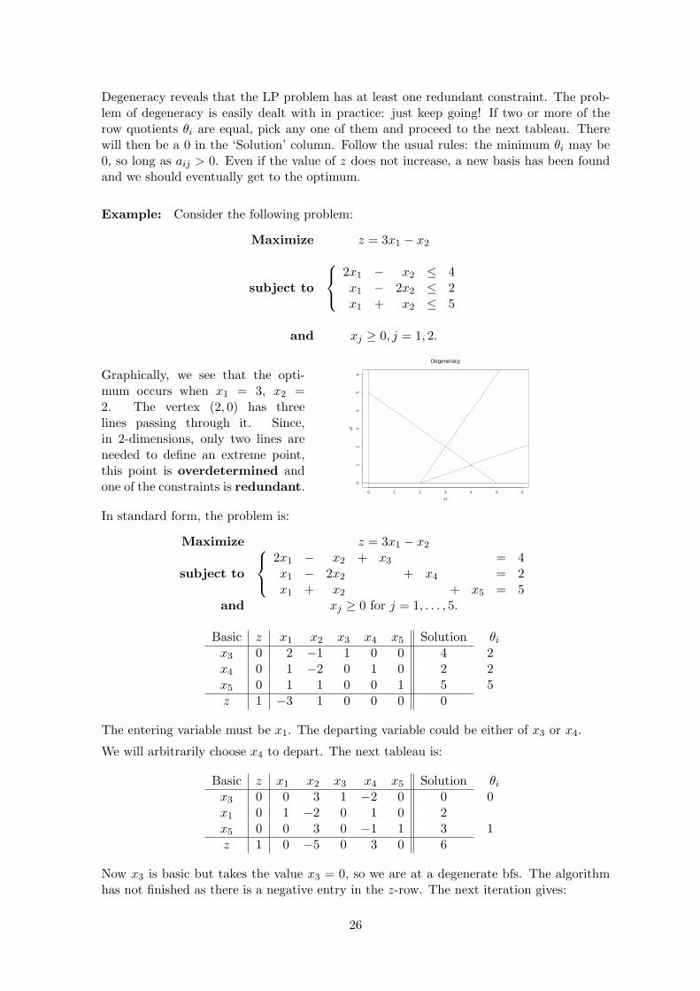
Example: Consider the following problem:

Maximize z = 3x1 − x2

subject to

2x1 − x2 ≤ 4x1 − 2x2 ≤ 2x1 + x2 ≤ 5

and xj ≥ 0, j = 1, 2.

Graphically, we see that the opti-mum occurs when x1 = 3, x2 =2. The vertex (2, 0) has threelines passing through it. Since,in 2-dimensions, only two lines areneeded to define an extreme point,this point is overdetermined andone of the constraints is redundant.

x1

x2

0 1 2 3 4 5 6

01

23

45

6

Degeneracy

In standard form, the problem is:

Maximize z = 3x1 − x2

subject to

2x1 − x2 + x3 = 4x1 − 2x2 + x4 = 2x1 + x2 + x5 = 5

and xj ≥ 0 for j = 1, . . . , 5.

Basic z x1 x2 x3 x4 x5 Solution θi

x3 0 2 −1 1 0 0 4 2x4 0 1 −2 0 1 0 2 2x5 0 1 1 0 0 1 5 5z 1 −3 1 0 0 0 0

The entering variable must be x1. The departing variable could be either of x3 or x4.

We will arbitrarily choose x4 to depart. The next tableau is:

Basic z x1 x2 x3 x4 x5 Solution θi

x3 0 0 3 1 −2 0 0 0x1 0 1 −2 0 1 0 2x5 0 0 3 0 −1 1 3 1z 1 0 −5 0 3 0 6

Now x3 is basic but takes the value x3 = 0, so we are at a degenerate bfs. The algorithmhas not finished as there is a negative entry in the z-row. The next iteration gives:

26

Basic z x1 x2 x3 x4 x5 Solution θi

x2 0 0 1 1/3 −2/3 0 0x1 0 1 0 2/3 −1/3 0 2x5 0 0 0 −1 1 1 3 3z 1 0 0 5/3 −1/3 0 6

This solution is degenerate again, and the objective function has not increased. There isstill a negative entry in the z-row. Pivoting on the x5 row gives:

Basic z x1 x2 x3 x4 x5 Solutionx2 0 0 1 −1/3 0 2/3 2x1 0 1 0 1/3 0 1/3 3x4 0 0 0 −1 1 1 3z 1 0 0 4/3 0 1/3 7

The algorithm has now terminated. zmax = 7 when x1 = 3, x2 = 2.

Both the second and third tableaux represent the point (2, 0, 0, 0, 3). The only difference isthat the decision variables are classified differently as basic and nonbasic at the two stages.

In a degenerate problem, it is possible (though unlikely) that the Simplex algorithm couldreturn at some iteration to a previous tableau. Once caught in this cycle, it will go roundand round without improving z.

Several methods have been proposed for preventing cycling. One of the simplest is the‘smallest subscript rule’ or ‘Bland’s rule’, which states that the simplex method will notcycle provided that whenever there is more than one candidate for the entering or leavingvariable, the variable with the smallest subscript is chosen (e.g. x3 in preference to x4).

2.4 Theory of the Simplex method

We now investigate the workings of the Simplex algorithm in more detail.

The initial and final tableaux for the rose growing problem were:

Initial tableau

Basic z x1 x2 x3 x4 x5 Solutionx3 0 5 4 1 0 0 6100x4 0 8 2 0 1 0 8000x5 0 1 5 0 0 1 5000z 1 −2 −3 0 0 0 0

Final tableau

Basic z x1 x2 x3 x4 x5 Solutionx1 0 1 0 5/21 0 −4/21 500x4 0 0 0 −38/21 1 22/21 2200x2 0 0 1 −1/21 0 5/21 900z 1 0 0 1/3 0 1/3 3700

In the initial tableau, the columns of the 4× 4 identity matrix occur in the columns headedx3, x4, x5, z respectively.

27

The corresponding columns in the final tableau, in the same order, form the matrix

P =

5/21 0 −4/21 0

−38/21 1 22/21 0−1/21 0 5/21 01/3 0 1/3 1

.

The entire initial tableau, regarded as a matrix, has been pre-multiplied by P to give theentire final tableau.

P tells us the row operations that would convert the initial tableau directly to the final

tableau, e.g. R2 := −3821

R1 + 1R2 +2221

R3 + 0R4.

In the final tableau, the columns of the 4 × 4 identity matrix occur under x1, x4, x2 and zrespectively. The corresponding columns of the initial tableau form the matrix

P−1 =

5 0 4 08 1 2 01 0 5 0

−2 1 −3 1

. This would pre-multiply the entire final tableau to give the

initial tableau.

To generalize this, suppose we are maximizing z = ctx subject to Ax ≤ b (where b ≥ 0)and x ≥ 0.

Let T1 be the initial simplex tableau, regarded as a matrix (i.e. omit the row and columnheadings) and let Tf be the final tableau.

T1 can be written in partitioned form as

0 A I b

1 −ct 0t 0

.

The final tableau is obtained from the initial one by a succesion of row operations, each ofwhich could be achieved by pre-multiplying T1 by some matrix. Hence Tf = PT1 for some

matrix P which can be partitioned in the form

M u

yt α

, say. As the z-column is

unchanged, u = 0 and α = 1.

The process of transforming the initial tableau to the optimal one can be expressed as: M 0

yt 1

0 A I b

1 −ct 0t 0

=

0 MA M Mb

1 ytA − ct yt ytb

.

Thus M and yt are found in the columns headed by the slack variables in the final tableau.

As Tf is optimal we must have y ≥ 0 and ytA − ct ≥ 0, i.e. Aty ≥ c.

Then zmax = ytb, or equivalently zmax = bty.

We shall meet these conditions again when we study the dual of a LP problem.

Now suppose that in the optimal tableau the basic variables, reading down the list in the

28

‘Basic’ column, are xB1, . . . , xBm and the non-basic variables are xN1, . . . , xNn. The initialtableau could be rearranged as follows:

Optimal basic variables Optimal non-basic variablesBasic z

︷ ︸︸ ︷xB1 · · · xBm

︷ ︸︸ ︷xN1 · · · xNn Solution

xn+1 0...

... B N bxn+m 0

z 1 −cB1 · · · − cBm −cN1 · · · − cNn 0

Thus the objective function can be written as

z = cB1xB1 + · · · + cBmxBm + cN1xN1 + · · · + cNnxNn.

Let cB = (cB1 · · · cBm)t, cN = (cN1 · · · cNn)t, xB = (xB1 · · · xBm)t, xN = (xN1 · · · xNn)t.

The process of transforming T1 (with the columns reordered as described) to Tf is now: M 0

yt 1

0 B N b

1 −cBt −cN

t 0

=

0 MB MN Mb

1 ytB − cBt ytN − cN

t ytb

.

The basic columns of the final tableau contain an identity matrix and a row of zeros soMB = I, i.e. M = B−1. Thus xB = B−1b.

Also ytB − cBt = 0 which can be written as yt = cB

tB−1.

Every entry in the z-row is non-negative at the optimum, so ytN − cNt ≥ 0,

i.e. cBtB−1N − cN

t ≥ 0. Then zmax = ytb = cBtB−1b. Thus we have:

Proposition 2.1 Let xB1, . . . , xBm be the basic variables in the optimal tableau for problem(LP1) with b ≥ 0. Let B be the matrix formed by the columns headed xB1, . . . , xBm in theinitial tableau (excluding the z-row). Then (xB1 · · · xBm)t = B−1b and zmax = cB

tB−1b.

2.4.1 Example

Consider the LP problem: Maximize z = 2x1 + 4x2 − 5x3, subject to

x1 + 2x2 + x3 ≤ 5, 2x1 + x2 − 4x3 ≤ 6, − 3x1 + 2x2 ≤ 3.

The initial and final tableaux are respectively:

Basic z x1 x2 x3 x4 x5 x6 Solutionx4 0 1 2 1 1 0 0 5x5 0 2 1 −4 0 1 0 6x6 0 −3 2 0 0 0 1 3z 1 −2 −4 5 0 0 0 0

Basic z x1 x2 x3 x4 x5 x6 Solutionx1 0 1 0 1/4 1/4 0 −1/4 1/2x5 0 0 0 −39/8 −7/8 1 3/8 11/4x2 0 0 1 3/8 3/8 0 1/8 9/4z 1 0 0 7 2 0 0 10

29

We now illustrate the theory set out in the last section.

30

We have been assuming that only extreme points of the feasible region need to be consideredas possible solutions. The proof of this is now given; you are not expected to learn it.

Proposition 2.2 v is a basic feasible solution of (LP2) if and only if v is an extreme pointof the set of feasible solutions S = {x : Ax = b, x ≥ 0} in Rn+m.

Proof (⇒) Suppose v is a bfs of (LP2) and is not an extreme point of S, so there aredistinct feasible solutions u, w ∈ S such that, for some r ∈ (0, 1),v = (1 − r)u + rw.

We can permute the columns of A, as described earlier, to get (B | N) and permute the

entries of v, u, w correspondingly so that(

vB

0

)= (1 − r)

(uB

uN

)+ r

(wB

wN

)As 0 < r < 1 and u,w are non-negative, it follows that uN = wN = 0.

As v, u, w are feasible, Av = Au = Aw = b,

so (B | N)(

vB

0

)= (B | N)

(uB

0

)= (B | N)

(wB

0

)= b.

Thus BvB = BuB = BwB = b. As B is non-singular, vB = uB = wB = B−1b.

Hence v = u = w, contradicting the assumption that these points are distinct, so v is anextreme point.

(⇐) Suppose v is in S, so is feasible, but is not a bfs of (LP2).

Av = b, so we can write (B′ | N′)(

v′

0

)= b, where v′ contains all the non-zero entries of

v. If v′ 6= v then B′ is not unique, but the following reasoning applies to any choice of B′.

If B′ were non-singular then v′ = B−1b, in which case v would be a bfs.

Hence B′ is singular, so there is a vector p such that B′p = 0.

As the entries of v′ are strictly positive, we can find ε > 0 so that v′ − εp ≥ 0 and

v′ + εp ≥ 0. Then B′(v′± εp) = B′v′± εA′p = B′v′±0 = b, so (B′ | N′)(

v′ ± εp0

)= b.

Thus both of(

v′ ± εp0

)are permuted feasible solution vectors. But

(v′

0

)is their

mean, so v is a convex linear combination of two points in S, hence v is not an extremepoint of S. It follows that any extreme point of S is a bfs of (LP2). �

31

Exercises 2

1. Use the Simplex method to solve

Maximize z = 4x1 + 8x2

subject to{

5x1 + x2 ≤ 83x1 + 2x2 ≤ 4

and x1 ≥ 0, x2 ≥ 0.

Express the objective function in terms of the non-basic variables in the final tableau,and hence explain how you know that the solution is optimal.

2. Use the Simplex method to solve

Maximize z = 5x1 + 4x2 + 3x3

subject to

2x1 + 3x2 + x3 ≤ 54x1 + x2 + 2x3 ≤ 113x1 + 4x2 + 2x3 ≤ 8

and xj ≥ 0 for j = 1, 2, 3.

Write down a matrix P which would pre-multiply the whole initial tableau to give thefinal tableau.

After you have studied Section 2.4 in the notes: write down, from the optimal tableauof this problem, the matrices B, B−1 and N and the vectors y, cB, cN as defined onpages 24 - 25. Verify that the optimal solution is B−1b and that zmax = cB

tB−1b.

3. Express the following LP problem in standard form. (Do not solve it.)

Minimize z = 2x1 + 3x2

subject to

x1 + x2 ≥ −1

2x1 + 3x2 ≤ 53x1 − 2x2 ≤ 3

and x1 unrestricted in sign, x2 ≥ 0.

4. The following tableau arose in the solution of a LP problem:

Basic z x1 x2 x3 x4 x5 x6 x7 Solution0 0 4/3 2/3 0 1 0 −1/3 40 0 1/3 2/3 1 0 1 −1/3 100 1 −1/3 1/6 1/2 0 0 1/6 4

z 1 0 −5/3 −4/3 −1 0 0 5/3 12

(a) Which variables are basic? What basic feasible solution does the tableau repre-sent? Is it optimal? Explain your answer by writing the z-row as an equation.

(b) Starting from the given tableau, proceed to find an optimal solution.

(c) From the optimal tableau, express the objective function and each of the basicvariables in terms of the non-basic variables.

32

5. Suppose one of the constraints in a LP problem is an equation rather than an inequal-ity, as in

Minimize 3x1 + 2x2 + 4x3

subject to

3x1 + 4x2 + 2x3 ≤ 63x1 + 5x2 + 7x3 ≤ 10x1 + x2 + x3 = 1

and x1 ≥ 0, x2 ≥ 0.

Use the third constraint to express x3 in terms of x1 and x2. Hence eliminate x3 fromthe objective function and the other two constraints. Introduce two slack variables x4

and x5, and solve the problem by the Simplex algorithm. Check that your solutionsatisfies all the constraints. How must this approach be modified if also x3 ≥ 0?

6. A furniture manufacturer makes chairs and settees, producing up to 80 chairs and48 settees per week. The items are sold in suites: Mini - two chairs, Family - threechairs and one settee, Grand - three chairs and two settees. The profits are £20, £30and £70 per suite, respectively. The total profit is to be maximized. Use the Simplexalgorithm to find the maximum profit that can be made in one week. State the profitand the number of each type of suite that should be made.

7. Solve the following problem using the simplex tableau method, making your deci-sion variable for I1 basic at the first iteration. Identify any degenerate basicfeasible solutions your calculations produce. Sketch the solution space and explainwhy degeneracy occurs.

A foundry produces two kinds of iron, I1 and I2, by using three raw materials R1, R2

and R3. Maximise the daily profit.

Raw Amount required per tonne Daily raw materialmaterial of I1 of I2 availability (tonnes)

R1 2 1 16R2 1 1 8R3 0 1 3.5

Profit per tonne £150 £300

8. Solve the following problem by the simplex algorithm, showing that every possiblebasic feasible solution occurs in the iterations.

Maximize z = 100x1 + 10x2 + x3

subject to

x1 ≤ 1

20x1 + x2 ≤ 100200x1 + 20x2 + x3 ≤ 10000

and x1 ≥ 0, x2 ≥ 0, x3 ≥ 0.

33

9. Consider the Linear Programming problem:

Maximize z = x1 + x2 + x3

subject to{

x1 + 3x2 − x3 ≤ 10x1 − x2 + 3x3 ≤ 14

and x1 ≥ 0, x2 ≥ 0, x3 ≥ 0.

Find a 3 × 3 matrix which would pre-multiply the initial tableau to give a tableauin which the basic variables are x1 and x3. Verify that this tableau is optimal, andhence state the solution of the problem.

If you had not been told which variables to take as basic, how many basic feasiblesolutions might you have to consider in order to solve the problem this way?

10. Prove that v is an extreme point of the feasible region R for (LP1) if and only if(v

b − Av

)is an extreme point of the feasible region S for (LP2).

34

Chapter 3

Further Simplex Methodology

3.1 Sensitivity analysis

Suppose some feature of a LP problem changes after we have found the optimal solution.Do we have to solve the problem again from scratch or can the optimum of the originalproblem be used as an aid to solving the new problem? These questions are addressed bysensitivity analysis, also called post-optimal analysis.

If a resource is used up completely then the slack variable in the constraint representing thisresource is zero, i.e. the constraint is active at the optimal solution. This type of resource iscalled scarce. In contrast, if the slack variable is non-zero (i.e. the constraint is not active)then this resource is not used up totally in the optimal solution. Resources of this kind arecalled abundant. Increasing the availability of an abundant resource will not in itself yieldan improvement in the optimal solution. However, increasing a scarce resource will improvethe optimal solution.

With the notation of Chapter 2, zmax = ytb. Suppose bi is increased by a small amountδbi. We say that the ith constraint has been relaxed by δbi. Then as long as the samevariables remain basic at the optimal solution, zmax = y1b1 + · · ·+ yi(bi + δbi)+ · · ·+ ymbm,i.e. zmax has increased by yiδbi.

yi is thus the approximate increase in the optimum value of z that results from allowing anextra 1 unit of the ith resource. yi is called the shadow price of the ith resource. It doesnot tell us by how much the resource can be increased while maintaining the same rate ofimprovement. If the set of constraints which are active at the optimal solution changes,then the shadow price is no longer applicable.

The shadow prices yi can be read directly from the optimal tableau: they are the numbersin the z-row at the bottom of the slack variable columns.

3.1.1 Example: the rose-growing problem modified

To illustrate these concepts we again consider the rose-growing problem, with the initialand final tableaux as obtained in Chapter 2.

The optimal solution is (500, 900, 0, 2200, 0). The slack variables x3, x4 and x5 were in-troduced in the land, finance and labour resource constraints respectively. Thus land andlabour are scarce resources, and finance is an abundant resource.

We now consider various modifications to the problem and its solution. Most of the methodsuse the multiplying matrix P which was defined in Section 2.4.

35

1. Shadow prices

2. Changing the resourcesThe rose grower has the option to buy some more land. What is the maximum areathat should be purchased if the other constraints remain the same?

36

3. Changing a coefficient in the objective functionThe profit margin alters on one of the roses. Is the same solution still optimal?

37

4. Adding an extra variable.

Suppose the grower has the option of growing an extra variety, pink roses, with thefollowing requirements per bush: 7 dm2 area, £6 finance, and 3.5 hours labour. Letthe profit per pink bush be £t, and suppose that x6 pink rose bushes are grown.

38

5. Adding an extra constraint.

Suppose the maximum number of roses that can be sold is 1340, so the constraintx1 + x2 ≤ 1340 is added to the system. The current optimum is not feasible asx1 + x2 = 500 + 900 > 1340.

Adding a slack variable x6 gives x1 + x2 + x6 = 1340.

39

The above procedure, keeping the z-row coefficients positive and carrying out row operationsuntil the basic variables are non-negative, is called the dual simplex method . It can beused, on its own or in combination with the normal simplex method, on problems whichare not quite in standard form because some of the right-hand sides are negative.

The dual simplex method provides one way of solving problems for which no initial basicfeasible solution is apparent. There are other variations on the simplex method which canbe used for such purposes, such as the Two-Phase method (see a textbook).

3.1.2 Example: the garments problem

A company makes three types of garment. The constraints are given by:Type A B C

No. of units x1 x2 x3 Amount availableLabour (hours) per unit 1 2 3 55 hoursMaterial (m2) per unit 3 1 4 80 m2

Profit (£) per unit 7 6 9

The company wants to make the largest possible profit subject to the constraints on

labour and materials, so they must ................................. z =

subject to

and x1 ≥ 0, x2 ≥ 0, x3 ≥ 0.

Adding slack variables, the constraints become:

Solve by the Simplex algorithm:

Basic z x1 x2 x3 x4 x5 Solution

z

Basic z x1 x2 x3 x4 x5 Solution

z

Basic z x1 x2 x3 x4 x5 Solution

z

Basic z x1 x2 x3 x4 x5 Solution

z

40

so the maximum profit is £when of type A, of type B and of type C are made.

From the initial to the final tableau, the middle two rows are multiplied by

B−1 =( )

. This is the inverse of B =( )

(using the columns for , respectively in the initial tableau.)

Taking cB =( )

, b =( )

,

cBtB−1b =

( )( )= = zmax.

We now consider the effect of changing some features of the problem.

1. Shadow prices

The shadow prices of labour and material are and respectively.

Both resources are ....................

The maximum profit increases at the rate of £ per extra hour of labour and£ per extra m2 of material, within certain limits.

2. Changing the resources

Suppose p hours of labour and q m2 of material are available.

The ‘solution’ column in the initial tableau is

so in the final tableau it is

=

.

For the solution to remain optimal when x1 > 0, x2 > 0, x3 = 0 we need

≥ 0 and ≥ 0, so

q ≤ and p ≤ . Thus ≤ q ≤If p is kept at 55, this gives ≤ q ≤Provided the amount of material is within this range, zmax =

when x1 = , x2 = , x3 =

When q = then zmax =

3. Changing a coefficient in the objective function

Suppose the profit on type A changes by £t per unit. This does not alter the feasibleregion, but it may affect the optimal solution.

The new objective function is z′ = ( )x1 + 6x2 + 9x3.

Thus the bottom row of the initial tableau is (1 | ................ − 6 − 9 0 0 || 0), soin the final tableau it is (1 | .............. 0 4 11/5 8/5 || 249).

For x1 to remain basic we must have 0 at the bottom of the x1 column, so add ........times Row ....... to Row ....... to get

41

(1 | .......... .......... .......... .............. .............. || ......................).

The original solution (21, 17, 0, 0, 0) is still optimal if no z-row entry is negative.

Therefore the original solution is optimal, with z′max = , provided

≥ 0, ≥ 0, ≥ 0, i.e. ≤ t ≤The profit on type A can vary from £ to £ without affecting the optimalquantities to produce.

4. Adding an extra variable.

Suppose the company can produce a fourth garment, type D, requiring 4 hours oflabour and 2 m2 of material and yielding £k profit per unit.

Let x0 units of type D be produced.

The new problem is to maximize z =

subject to

= 55, = 80,

where xj ≥ 0 for j = 0, . . . , 5.

The initial tableau is as before with the addition of a column

x0

3/5 −1/5 0−1/5 2/5 011/5 8/5 1

=

, so we have

x0

in the final tableau.

Thus if k ≤ , the z-row remains non-negative and the current solution is optimal;D should not be made.

Suppose we take k = 13. Then the previously optimal tableau becomes

Basic z x0 x1 x2 x3 x4 x5 Solutionx2 0 0 1 1 3/5 −1/5 17x1 0 1 0 1 −1/5 2/5 21z 1 0 0 4 11/5 8/5 249

After one more iteration this becomes optimal:

Basic z x0 x1 x2 x3 x4 x5 Solution0

0z 1

so units of A and units of D should be made.

(If half-units are not possible, Integer Programming is needed.)

42

5. Adding an extra constraint.

Suppose that in the original 3-product problem there is a further restriction:3x1 + x2 + 2x3 ≤ 50, i.e. 3x1 + x2 + 2x3 + x6 = 50 where x6 ≥ 0 is a slack variable.

3(21) + 17 + 2(0) > 50, so the previous optimal point (21, 17, 0) is not feasible.

Adding the new constraint as a row in the original optimal tableau gives:

Basic z x1 x2 x3 x4 x5 x6 Solution0 0 1 1 3/5 −1/5 0 170 1 0 1 −1/5 2/5 0 21

x6 0z 1 0 0 4 11/5 8/5 0 249

This does not represent a valid Simplex iteration because there is only one basiccolumn. Subtracting Row 1 and 3 times Row 2 from Row 3 gives:

Basic z x1 x2 x3 x4 x5 x6 Solutionx2 0 0 1 1 3/5 −1/5 0 17x1 0 1 0 1 −1/5 2/5 0 21x6 0z 1 0 0 4 11/5 8/5 0 249

This represents a basic but infeasible solution. It would be optimal if the negativeentry in the solution column were not there. In this situation we use the dual simplexmethod, as described on page 40.

x6 = , so x6 must leave leave the basis.

To keep the z-row entries non-negative, choose the entering variable as follows:

Where there is a negative number in the pivot row, divide the z-row entry by this andchoose the variable for which the modulus of this quotient is smallest.

| ÷ | < | ÷ | so enters the basis.

Basic z x1 x2 x3 x4 x5 x6 Solutionx2 0x1 0

0z 1

Making of type A and of type B is now optimal, giving profit £

3.2 The dual simplex method

The method that we used above when negative numbers occur in the solution column canbe used on any such problems, not just in the context of sensitivity analysis.

The differences between the original simplex method and the dual simplex method can besummarised as follows:

43

Original (‘primal’) simplex Dual simplex• Starts from a basic feasible solution. • Starts from a basic infeasible solution.• All bj ≥ 0. • At least one bj < 0.• At least one z-row entry is negative. • All z-row entries ≥ 0.• Seek to make all z-row entries ≥ 0 • Seek to make all bj ≥ 0 keeping the z-row ≥ 0.

The algorithm is:

1. Express the problem in maximization form with slack variables (not in standard form).

2. Find the most negative number in the ‘solution’ column. Suppose this is in row i.

3. For each negative aij in row i, find the smallest absolute value∣∣∣∣ cj

aij

∣∣∣∣.4. Use aij as the pivot in the usual way to obtain a new tableau.

5. Return to step 2. Continue until there are no negative entries in the solution columnor the z-row.

3.2.1 Example

Use the dual simplex algorithm to solve the problem:

Minimize z = 5x1 + 4x2

subject to{

3x1 + 2x2 ≥ 6x1 + 2x2 ≥ 4

and x1 ≥ 0, x2 ≥ 0.

44

3.3 The dual of a Linear Programming problem

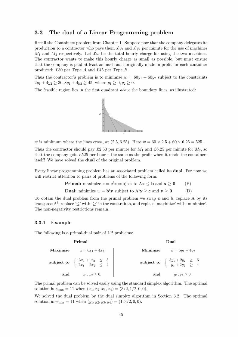
Recall the Containers problem from Chapter 1. Suppose now that the company delegates itsproduction to a contractor who pays them £y1 and £y2 per minute for the use of machinesM1 and M2 respectively. Let £w be the total hourly charge for using the two machines.The contractor wants to make this hourly charge as small as possible, but must ensurethat the company is paid at least as much as it originally made in profit for each containerproduced: £30 per Type A and £45 per Type B.

Thus the contractor’s problem is to minimize w = 60y1 + 60y2 subject to the constraints2y1 + 4y2 ≥ 30, 8y1 + 4y2 ≥ 45, where y1 ≥ 0, y2 ≥ 0.

The feasible region lies in the first quadrant above the boundary lines, as illustrated:

0

2

4

6

8

10

12

14

y2

2 4 6 8 10 12 14 16 18

y1

w is minimum where the lines cross, at (2.5, 6.25). Here w = 60 × 2.5 + 60 × 6.25 = 525.

Thus the contractor should pay £2.50 per minute for M1 and £6.25 per minute for M2, sothat the company gets £525 per hour – the same as the profit when it made the containersitself! We have solved the dual of the original problem.

Every linear programming problem has an associated problem called its dual. For now wewill restrict attention to pairs of problems of the following form:

Primal: maximize z = ctx subject to Ax ≤ b and x ≥ 0 (P)

Dual: minimize w = bty subject to Aty ≥ c and y ≥ 0 (D)

To obtain the dual problem from the primal problem we swap c and b, replace A by itstranspose At, replace ‘≤’ with ‘≥’ in the constraints, and replace ‘maximize’ with ‘minimize’.The non-negativity restrictions remain.

3.3.1 Example

The following is a primal-dual pair of LP problems:

Primal

Maximize z = 6x1 + 4x2

subject to{

3x1 + x2 ≤ 52x1 + 2x2 ≤ 4

and x1, x2 ≥ 0.

∣∣∣∣∣∣∣∣∣∣∣∣

Dual

Minimize w = 5y1 + 4y2

subject to{

3y1 + 2y2 ≥ 6y1 + 2y2 ≥ 4

and y1, y2 ≥ 0.

The primal problem can be solved easily using the standard simplex algorithm. The optimalsolution is zmax = 11 when (x1, x2, x3, x4) = (3/2, 1/2, 0, 0).

We solved the dual problem by the dual simplex algorithm in Section 3.2. The optimalsolution is wmin = 11 when (y1, y2, y3, y4) = (1, 3/2, 0, 0).

45

Notice that the objective functions of the primal and dual problems have the same optimumvalue. Furthermore, in the optimal dual tableau, the objective row coefficients of the slackvariables are equal to the optimal primal decision variables.

Consider the cattle-feed problem in Chapter 1. Suppose a chemical company offers thefarmer synthetic nutrients at a cost of £y1 per unit of protein, £y2 per unit of fat, £y3 perunit of calcium and £y4 per unit of phosphorus.

The cost per unit of hay substitute is thus £(13.2y1+4.3y2+0.02y3+0.04y4). To be economicto the farmer, this must not be more than £0.66. Similarly, considering the oats substitute,34.0y1 + 5.9y2 + 0.09y3 + 0.09y4 ≤ 2.08.

For feeding one cow, the company will receive £(65.0y1 + 14.0y2 + 0.12y3 + 0.15y4), whichit will wish to maximize.

Thus the company’s linear programming problem is :

Maximize w = 65.0y1 + 14.0y2 + 0.12y3 + 0.15y4

subject to{

13.2y1 + 4.3y2 + 0.02y3 + 0.04y4 ≤ 0.6634.0y1 + 5.9y2 + 0.09y3 + 0.09y4 ≤ 2.08

and yj ≥ 0, j = 1, ..., 4.

We see that the dual of this is the farmer’s original problem. As we shall show next, in factthe two problems are the duals of each other.

Proposition 3.1 The dual of the dual problem (D) is the primal problem (P).

Proof The dual problem (D) can be written as follows:

maximize (−b)ty subject to (−A)ty ≤ −c and y ≥ 0.

The dual of this is:

minimize (−c)tx subject to (−At)tx ≥ −b and x ≥ 0.

This is equivalent to:

maximize ctx subject to Ax ≤ b and x ≥ 0,

which is the same as the primal problem (P).

Thus the dual of either problem may be constructed according to the following rules:

Primal DualMaximize ctx Minimize btyMinimize ctx Maximize btyConstraints Ax ≥ b Constraints Aty ≤ cConstraints Ax ≤ b Constraints Aty ≥ cx ≥ 0 y ≥ 0.

• For every primal constraint there is a dual variable.

46

• For every primal variable there is a dual constraint.

• the constraint coefficients of a primal variable form the left-side coefficients of thecorresponding dual constraint; the objective coefficient of the same variable becomesthe right-hand side of the dual constraint.

We now investigate how the solutions of the primal and dual problems are related, so thatby solving one we automatically solve the other.

Proposition 3.2 (The weak duality theorem) Let x be any feasible solution to the pri-mal problem (P) and let y be any feasible solution to the dual problem (D).

(i) ctx ≤ bty.

(ii) If ctx = bty then x and y are optimal solutions to the primal and dual problems.

Proof

(i) As x and y are feasible, we have Ax ≤ b, Aty ≥ c, x ≥ 0, y ≥ 0.

Thus ctx ≤ (Aty)tx = ytAx ≤ ytb = bty.

(ii) Suppose ctx = bty. If ctx0 > ctx for any primal feasible x0, then ctx0 > bty whichcontradicts (i). Hence ctx0 ≤ ctx for all primal feasible x0, so x is optimal for (P). Similarly,y is optimal for (D).

Proposition 3.3 (The strong duality theorem) If either the primal or dual problemhas a finite optimal solution, then so does the other, and the optimum values of the primaland dual objective functions are equal, i.e. zmax = wmin.

Proof

Let x be a finite optimal solution to the primal, so that zmax = ctx = z∗ say.

We have seen that the initial tableau is pre-multiplied as follows to give the final tableau:

B−1 0

yt 1

A I b

−ct 0t 0

=

B−1A B−1 B−1b

ytA − ct yt ytb

.

As this is optimal, ytA − ct ≥ 0, so Aty ≥ c,

and y ≥ 0. Hence y is feasible for the dual problem.

Now z∗ = ytb = bty.

But also z∗ = ctx so x,y are feasible solutions which give equal values of the primal anddual objective functions respectively.

Thus by Proposition 3.2 (ii), x,y are optimal solutions and z∗ is the optimal value of bothz and w.

As each problem is the dual of the other, the same reasoning applies if we start with a finiteoptimal solution y to the dual.

The above shows that the entries of y are in fact the optimal values of the main variablesin the dual problem. (They are also the shadow prices for the primal constraints).

47

Furthermore the entries of ytA − ct are the values of the dual surplus variables at theoptimum, so we shall denote them by ym+1, . . . , ym+n.

Thus the optimal primal tableau contains the following information:

Primal main Primal slackBasic z

︷ ︸︸ ︷x1 · · · xn

︷ ︸︸ ︷xn+1 · · · xn+m Solution

Primal 0 Values ofbasic · primal basic

variables 0 variablesz 1 ym+1 · · · ym+n︸ ︷︷ ︸ y1 · · · ym︸ ︷︷ ︸ Optimum of objective

Values of dual Values of dual functions (primal and dual)surplus variables main variables

The optimal dual solutions may therefore be read from the optimal primal tableau withoutfurther calculations. Furthermore, since the dual of the dual is the primal, it does not matterwhich problem we solve – the optimal solution of one will give us the optimal solution ofthe other. This is important, as if we are presented with a ‘difficult’ primal problem, it maybe easier to solve it by tackling its dual:

• if the primal constraints are all of the ‘≥’ form then (P) cannot be solved by thenormal simplex algorithm, but (D) can;

• if the primal problem has many more constraints than variables then the dual hasmany fewer constraints than variables, and will in general be quicker to solve.

Proposition 3.4 If either the primal (P) or the dual (D) has an unbounded optimal solu-tion then the other has no feasible solution.

Proof: Suppose the dual has a feasible solution y. Then for any primal feasible solutionx, ctx ≤ bty, so bty is an upper bound on solutions of the primal. Similarly, if the primalhas a feasible solution this places a lower bound on solutions of the dual. It follows that ifeither problem is unbounded then the other does not have a feasible solution.

Proposition 3.4 identifies some cases where the duality results do not hold, i.e. we cannotsay that the primal and dual LP problems have the same optimal values of their objectivefunctions:

1. Primal problem unbounded and dual problem infeasible.

2. Primal problem infeasible and dual problem unbounded.

3. Primal and dual problems both infeasible.

3.4 Complementary slackness

Complementary slackness is a very important and useful consequence of the relationshipbetween the primal and dual optima. We continue to work with the primal-dual pair (P)and (D).

In the final tableau for the primal problem, if xi is non-basic then xi = 0 at the optimum.

48

Let the primal problem have n main variables and m constraints. Suppose the main variablexi is basic in the optimal tableau. Then there is a zero in the z row at the bottom of thexi column, so the dual surplus variable ym+i is zero at the optimum.

We see that for i = 1, . . . , n, either xi = 0 or ym+1 = 0.

Also, if xn+j is a slack variable in the primal problem then the corresponding dual variableis the main variable yj . For j = 1, . . . ,m, either yj = 0 or xn+j = 0.

Thus in every case xiym+i = 0 and xn+jyj = 0.

So at the optimal solution,

ith primal main variable × ith dual surplus variable = 0,jth primal slack variable × jth dual main variable = 0.

These relationships are called the complementary slackness equations.

Thus (x1 · · · xn | xn+1 · · · xn+m)(ym+1 · · · ym+n | y1 · · · ym)t = 0, since the scalar productof two non-negative vectors is 0 iff the product of each corresponding pair of entries is 0.

Now the entries of b−Ax are the primal slack variables xn+1, . . . , xn+m and the entries ofAty − c are the dual surplus variables ym+1, . . . , ym+n, so complementary slackness assertsthat at the optimal solution,

yt(b − Ax) = 0 and xt(Aty − c) = 0.

An interpretation of complementary slackness is that if the shadow price of a resource isnon-zero then the associated constraint is active at the optimum, i.e. the resource is scarce,but if the constraint is not active (the resource is abundant) then its shadow price is zero.

Proposition 3.5 (The complementary slackness theorem) A necessary and sufficientcondition for x and y to be optimal for the primal and dual problems (P) and (D) is thatx is primal feasible, y is dual feasible, and x and y satisfy the complementary slacknessconditions yt(b − Ax) = 0 and xt(Aty − c) = 0.

Proof:

By the duality theorems, x and y are optimal iff they are feasible and ctx = bty.

Now ctx = bty ⇔ ytb − xtc = 0

⇔ ytb − ytAx + xtAty − xtc = 0 (since ytAx = xtAty)

⇔ yt︸︷︷︸≥0

(b − Ax)︸ ︷︷ ︸≥0

+ xt︸︷︷︸≥0

(Aty − c)︸ ︷︷ ︸≥0

= 0

⇔ yt(b − Ax) = 0 and xt(Aty − c) = 0.

3.4.1 Examples

1. Consider the rose-growing problem in Chapter 1. The solution of this was

(x1, x2, x3, x4, x5) = (500, 900, 0, 2200, 0).

The dual problem is : Minimize w = 6100y1 + 8000y2 + 5000y3

subject to 5y1 + 8y2 + y3 ≥ 2, 4y1 + 2y2 + 5y3 ≥ 3, yi ≥ 0 for i = 1, 2, 3.

By the strong duality theorem we know that the minimum value of w is the same asthe maximum of z in the primal problem, namely 3700. We can read off from the final

49

tableau that y1 = y3 = 1/3, y2 = y4 = y5 = 0, where y4, y5 are the surplus variablesin the two constraints of the dual.

If we solved the primal problem graphically, we would only know x1 = 500, x2 = 900.

Complementary slackness then tells us that x1y4 = x2y5 = x3y1 = x4y2 = x5y3 = 0so 500y4 = 900y5 = 0y1 = 2200y2 = 0y3 = 0, and since all the yj are ≥ 0 it followsthat y2 = y4 = y5 = 0. Thus both dual constraints are active at the optimum, so5y1 + y3 = 2, 4y1 + 5y3 = 3. Solving these gives y1 = y3 = 1/3.

2. Suppose we wish to verify that (x1, x2) = (10, 5) maximizes z = 30x1 + 45x2 subjectto the constraints in the Containers Problem of Chapter 1. (10, 5) is certainly feasiblefor the primal, i.e. it satisfies the constraints. Then z = 525.

The dual is: Minimize w = 60y1 + 60y2 subject to 2y1 + 4y2 ≥ 30, 8y1 + 4y2 ≥ 45,y1 ≥ 0, y2 ≥ 0. When equality holds in both constraints, y1 = 5/2 and y2 = 25/4.

Thus (x1, x2, x3, x4) = (10, 5, 0, 0) is primal feasible, (y1, y2, y3, y4) = (5/2, 25/4, 0, 0)is dual feasible, and (10, 5, 0, 0).(0, 0, 5/2, 25/4) = 0, i.e. the complementary slacknessconditions hold. By Theorem 3.5, these solutions are optimal for the primal and dualproblems.

We can further check that when y1 = 5/2 and y2 = 25/4, w = 525.

3. Consider again the Cattle Feed problem and its dual from Chapter 1. From theoriginal solution, zmin = 3.46 when x1 = 3.48, x2 = 0.56. If x3, x4, x5, x6 are thesurplus variables in the four constraints, then x3 = x5 = 0 at the optimum as the firstand third constraint are active, but x4, x6 are non-zero.

Let y5, y6 be the slack variables in the two dual constraints. By complementaryslackness, (x1, x2, | x3, x4, x5, x6).(y5, y6, | y1, y2, y3, y4) = 0. Thus y2 = y4 = y5 =y6 = 0 at the dual optimum.

Hence 13.2y1 + 0.02y3 = 0.66, 34.0y1 + 0.09y3 = 2.08, and solving these gives

y1 = 0.035, y3 = 9.87.

We conclude that the company should charge £0.035 per unit of synthetic protein,£9.87 per unit of synthetic calcium, give away synthetic fat and phosphorus free,and thus charge £3.46 for feeding one cow. No price structure can bring them ahigher income without costing the farmer more than before. In accordance with theStrong Duality Theorem, if the farmer and the company both behave rationally (i.e.optimally) then the costs of the normal and synthetic feeding plans are the same. Ofcourse, in practice other considerations might influence the farmer’s decision.

If we solved the dual problem by the simplex algorithm, the solutions for x1, . . . , x6

in the primal problem could be read off from the bottom row of the optimal tableau.

The complementary slackness conditions have the following interpretation here:

(a) If (Ax)i < bi then yi = 0. This means the farmer should buy zero of any nutrientthat is overpriced compared to its synthetic equivalent.

(b) If (Aty)j > cj then xj = 0. Thus the company should charge zero for anynutrient that is over-supplied in the normal feeding plan.

50

3.5 Asymmetric duality

The dual problems in Equations (P) and (D) are said to represent symmetric duality.We now examine the situation where the variables in the primal problem are unrestrictedin sign. Thus the primal problem is:

Maximize z = ctx subject to Ax ≤ b, x unrestricted. (AP)

We can convert this into a LP problem in standard form by letting x = x′ − x′′, wherex′ ≥ 0 and x′′ ≥ 0.

The constraints then become A(x′ − x′′) ≤ b.

This can be written as (A | − A)x ≤ b, where x = (x′1 · · · x′

n x′′1 · · · x′′

n)t.

The objective function is z = ctx′ − ctx′′ = (ct | − ct)x, and clearly x ≥ 0.

Thus the problem becomes

Maximize z = (ct | − ct)x subject to (A | − A)x ≤ b, x ≥ 0.

The dual of this problem can be written as:

Minimize w = bty subject to(

At

−At

)y ≥

(c−c

), y ≥ 0.

Now if −Aty ≥ −c then Aty ≤ c. If this is true simultaneously with Aty ≥ c then we musthave Aty = c. Thus the dual of the unrestricted problem (AP) is

Minimize w = bty subject to Aty = c, y ≥ 0. (AD)

Conversely, the dual of (AD), a problem with equality constraints, is (AP), a problem inwhich the variables are unrestricted. (Of course, every LP problem can be expressed as onewith equality constraints by including slack and surplus variables.)

Proposition 3.6 The following two problems are duals of each other:

Maximize z = ctx subject to Ax ≤ b, x unrestricted,

Minimize w = bty subject to Aty = c, y ≥ 0.

3.5.1 Example

Consider the following asymmetric pair of primal-dual problems:

Primal

Maximize z = x1 − 2x2

subject to{

x1 + x2 ≤ 4−2x1 − 3x2 ≤ −5

and x1, x2 unrestricted.

∣∣∣∣∣∣∣∣∣∣∣∣

Dual

Minimize w = 4y1 − 5y2

subject to{

y1 − 2y2 = 1y1 − 3y2 = −2

and y1, y2 ≥ 0.

Clearly a solution of the dual can occur only where the two equations hold, i.e. wheny1 = 7, y2 = 3. Thus w has a minimum value of 13, and this must also be the maximumvalue of z in the primal problem. By complementary slackness we find that x1 = 7, x2 = −3.

51

Exercises 3

1. A company which manufactures three products A, B and C, needs to solve the fol-lowing LP problem in order to maximize their profit.

Maximize z = 3x1 + x2 + 5x3

subject to{

6x1 + 3x2 + 5x3 ≤ 453x1 + 4x2 + 5x3 ≤ 30

and xj ≥ 0 for j = 1, 2, 3.

x1, x2 and x3 are the amounts of A, B and C to be produced. The first constraint isa labour constraint, and the second is a material constraint. The company solves theproblem and obtains an optimal solution in which x1 and x3 are basic.

(a) Find the company’s optimal solution.(b) How much can c2, the unit profit for B, be increased above 1 without affecting

the original optimal solution?(c) Find the range of values of c1, the unit profit for A, for which x1 and x3 are still

basic at the optimal solution. When this is the case, express the maximum valueof z in terms of c1.

(d) Find an optimal solution when b2, the amount of material available, is 60 units.(e) The constraint 3x1 + 2x2 + 3x3 ≤ 25 is added to the original problem. How does

this affect the original optimal solution?(f) A new product D has a unit profit of 5, and its labour and material requirements

are 3 units and 4 units respectively. Is it profitable to produce D?(g) An additional 15 units of material are available for £10. What should be done?

2. A firm can manufacture four products at its factory. Production is limited by themachine hours available and the number of special components available. The dataare given in the table below. Note that production of fractions of a unit is possible.

Product Availability1 2 3 4

Machine hours per unit 1 3 8 4 Up to 90 machine hours per dayComponents per unit 2 2 1 3 Up to 80 components per dayProduction costs (£ per unit) 20 25 40 55Sales income (£ per unit) 30 45 80 85

(a) Formulate this as a linear programming problem, where xj is the daily productionof product j and the objective is to maximize the daily profit (income minusproduction costs). Find the optimal solution using the simplex tableau method,and state the optimal profit.

(b) Write down the shadow prices of machine hours and components, briefly explain-ing their significance.

(c) The firm can increase the available machine hours by up to 10 hours per day byhiring extra machinery. The cost of this would be £40 per day. Use sensitivityanalysis to decide whether they should hire it, and if so, find the new productionschedule.

52

(d) The production costs of products 1 and 4 are changed by £t per unit. Withinwhat range of values can t lie if the original production schedule is to remainoptimal? Find the corresponding range of values of the maximum profit.

(e) Due to a problem at the distributors, the total daily amount produced has tobe limited to 25 units. Implement the dual simplex algorithm to find a newproduction schedule which meets this restriction.

(f) After production has returned to normal (i.e. the original solution is optimalagain) the firm considers manufacturing a new product that would require 3 ma-chine hours and 4 components per unit. The production costs would be £45 andsales income £75 per unit. Use sensitivity analysis to decide whether they shouldgo ahead, and if so what the optimum production schedule would be.

3. In each case formulate the dual problem and verify that the given solution is optimalby showing that primal feasibility, dual feasibility and complementary slackness allhold.

(a) Maximize 19x1 + 16x2 subject to the constraints x1 + 4x2 ≤ 20, 3x1 + 2x2 ≤ 15,

x1 ≥ 0, x2 ≥ 0. Solution (x1, x2) = (2, 9/2)

(b) Minimize 8x1 + 11x2 subject to the constraints 2x1 − 2x2 ≥ 2, x1 + 4x2 ≥ −5,

x1 ≥ 0, x2 ≥ 0. Solution (x1, x2) = (1, 0)

4. The optimal solution of the problem

Maximize 6x1 + 4x2 + 10x3

subject to

x1 + 2x2 + x3 ≤ 20

3x1 + 2x3 ≤ 242x1 + 2x2 ≤ 22

and x1, x2, x3 ≥ 0.

occurs at (x1, x2, x3) = (0, 4, 12). Deduce the solution of the dual problem.

5. Formulate the dual of each of the two problems in Section 2.2.1 and solve them fromthe optimal primal tableaux using the theory of duality and complementary slackness.

6. By finding and solving the dual problem (without using the simplex algorithm), findthe maximum value of

z = 5x1 + 7x2 + 8x3 + 4x4

subject to x1 + x3 ≤ 6, x1 + 2x4 ≤ 5, x2 + x3 ≤ 9, x2 + x4 ≤ 3, where x1, x2, x3, x4 areunrestricted in sign.

7. Use asymmetric duality to find the solutions (if any) of the following LP problems:

(a)Maximize z = x1 + 2x2

subject to{

2x1 − 3x2 ≤ 1x1 + 4x2 ≤ 5

and x1, x2 unrestricted.

53

(b)Maximize z = 3x1 + 7x2 + 5x3

subject to{

2x1 + 5x2 + 4x3 ≤ 92x1 + 4x2 + 2x3 ≥ 7

and x1, x2, x3 unrestricted.

8. When the problem

Maximize 12x1 + 6x2 + 4x3

subject to

4x1 + 2x2 + x3 ≤ 602x1 + 3x2 + 3x3 ≤ 50x1 + 3x2 + x3 ≤ 45

and x1, x2, x3 ≥ 0.

is solved by the simplex method, using slack variables x4, x5, x6 respectively in thethree constraints, the final tableau is

Basic z x1 x2 x3 x4 x5 x6 Solutionx1 0 1 3/10 0 3/10 −1/10 0 13x3 0 0 4/5 1 −1/5 2/5 0 8x6 0 0 19/10 0 −1/10 −3/10 1 24z 1 0 4/5 0 14/5 2/5 0 188

(a) State the optimal solution and the values of x1, . . . , x6 at the optimum.(b) Write down the dual problem, using y1, y2, y3 for the dual main variables and

y4, y5, y6 for the dual surplus variables.(c) Using the above tableau, write down the optimal solution of the dual problem

and give the values of y1, . . . , y6 at the optimum.(d) Show how complementary slackness occurs in these solutions.(e) Convert the dual problem to a maximization problem and solve it by the Dual

Simplex method.(f) Comment on the relationships between the two optimal tableaux.

9. By solving the dual problem graphically, solve the LP problem:

Minimize 4x1 + 3x2 + x3

subject to{

3x1 + 8x2 + 2x3 ≥ 32x1 + 5x2 + 3x3 ≥ 5

and x1, x2, x3 ≥ 0.

Give the values of all the dual and primal variables (main, slack and surplus) at theoptimum.

10. Find the dual of the problem

Maximize ctx subject to Ax = b, x ≥ 0.

54

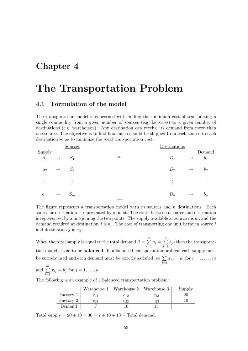
Chapter 4

The Transportation Problem

4.1 Formulation of the model

The transportation model is concerned with finding the minimum cost of transporting asingle commodity from a given number of sources (e.g. factories) to a given number ofdestinations (e.g. warehouses). Any destination can receive its demand from more thanone source. The objective is to find how much should be shipped from each source to eachdestination so as to minimize the total transportation cost.

Sources DestinationsSupply Demand

a1 → S1c11 D1 → b1

a2 → S2 D2 → b2

......

......

am → Sm Dn → bncmn

The figure represents a transportation model with m sources and n destinations. Eachsource or destination is represented by a point. The route between a source and destinationis represented by a line joining the two points. The supply available at source i is ai, and thedemand required at destination j is bj . The cost of transporting one unit between source iand destination j is cij .

When the total supply is equal to the total demand (i.e.m∑

i=1ai =

n∑j=1

bj) then the transporta-

tion model is said to be balanced. In a balanced transportation problem each supply must

be entirely used and each demand must be exactly satisfied, son∑

j=1xij = ai for i = 1, . . . , m

andm∑

i=1xij = bj for j = 1, . . . , n.

The following is an example of a balanced transportation problem:

Warehouse 1 Warehouse 2 Warehouse 3 SupplyFactory 1 c11 c12 c13 20Factory 2 c21 c22 c23 10Demand 7 10 13

Total supply = 20 + 10 = 30 = 7 + 10 + 13 = Total demand.

55

A transportation model in which the total supply and total demand are not equal is calledunbalanced. It is always possible to balance an unbalanced transportation problem.

Suppose the demand at warehouse 1 above is 9 units. Then the total supply and totaldemand are unequal, and the problem is unbalanced. In this case it is not possible tosatisfy all the demand at each destination simultaneously.

We modify the model as follows: since demand exceeds supply by 2 units we introduce adummy source, Factory 3, which has a capacity of 2. The amount sent from this dummysource to a destination represents the shortfall at that destination.

If supply exceeds demand then a dummy destination, Warehouse 4, is introduced toabsorb the surplus units. Any units shipped from a source to a dummy destination representa surplus at that source.

Transportation costs for dummy sources or destinations are allocated as follows:

• If a penalty cost is incurred for each unit of unsatisfied demand or unused supply,then the transportation cost is set equal to the penalty cost.

• If there is no penalty cost, the transportation cost is set equal to zero.

• If no units may be assigned to a dummy or a particular route, allocate a cost M . Thisrepresents a number larger than any other in the problem – think of it as a million!

From now on we shall consider balanced transportation problems only, as any unbalancedproblem can be balanced by introducing a dummy.

Let xij denote the amount transported from source i to destination j. Then the problem is

Minimize z =m∑

i=1

n∑j=1

cijxij ,

subject ton∑

j=1

xij = ai for i = 1, . . . , m

andm∑

i=1

xij = bj for j = 1, . . . , n,

where xij ≥ 0 for all i and j.

4.2 Solution of the transportation problem

A balanced transportation problem hasm∑

i=1ai =

n∑j=1

bj . Hence one constraint is a linear

combination of the others, so there are n + m − 1 independent constraint equations.

It is not practicable to use the standard simplex method to solve the transportation problem.However, there is an efficient tableau-based method which makes use of the dual problem.

Starting the algorithm: finding an initial basic feasible solution

Here we examine ways of constructing initial basic feasible solutions, i.e. allocations withm + n − 1 basic variables.

56

Method 1: The North-West Corner Method

Consider the problem represented by the following transportation tableau. The numberin the bottom right of cell (i, j) is cij , the cost of transporting 1 unit from source i todestination j.

Supply

10 0 20 1115

12 7 9 2025

0 14 16 185

Demand 5 15 15 10

The north-west corner method proceeds as follows:

• Assign as much as possible to the cell in the top-left of the tableau.

• Cross out the row or column whose supply or demand is satisfied. If a row and columnare both satisfied then cross out only one of them.

• Adjust the supply and demand for those rows and columns which are not crossed out.

• Repeat the above steps on the remaining tableau until only one row or column remains.

The values of the basic variables xij are entered in the top left of each cell. There shouldalways be m+n−1 of these; in certain (degenerate) cases some of them may be zero. Theymust always add up to the total supply and demand in each row and column.

Note that some books position the data differently in the cells of the tableau.

Method 2: The Least-Cost Method

This method usually provides a better initial basic feasible solution than the North-WestCorner method. Despite its name, it does not give the actual minimum cost. It uses leastavailable costs to obtain a starting tableau.

57

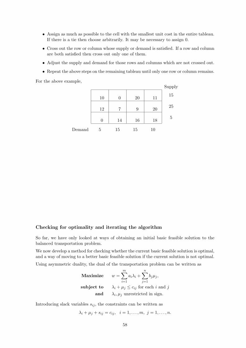
• Assign as much as possible to the cell with the smallest unit cost in the entire tableau.If there is a tie then choose arbitrarily. It may be necessary to assign 0.

• Cross out the row or column whose supply or demand is satisfied. If a row and columnare both satisfied then cross out only one of them.

• Adjust the supply and demand for those rows and columns which are not crossed out.

• Repeat the above steps on the remaining tableau until only one row or column remains.

For the above example,Supply

10 0 20 1115

12 7 9 2025

0 14 16 185

Demand 5 15 15 10

Checking for optimality and iterating the algorithm

So far, we have only looked at ways of obtaining an initial basic feasible solution to thebalanced transportation problem.

We now develop a method for checking whether the current basic feasible solution is optimal,and a way of moving to a better basic feasible solution if the current solution is not optimal.

Using asymmetric duality, the dual of the transportation problem can be written as

Maximize w =m∑

i=1

aiλi +n∑

j=1

bjµj ,

subject to λi + µj ≤ cij for each i and j

and λi, µj unrestricted in sign.

Introducing slack variables sij , the constraints can be written as

λi + µj + sij = cij , i = 1, . . . , m, j = 1, . . . , n.

58

By the complementary slackness conditions we must have xijsij = 0, i.e.

xij (cij − λi − µj) = 0 for all i and j.

As before, primal feasibility, dual feasibility and complementary slackness are necessary andsufficient for optimality. This is the underlying strategy for solving the problem.

For illustrative purposes, we shall start the algorithm for the above example using the bfsthat was provided by the North-West Corner method. The Least-Cost method will usuallygive a better initial allocation.

We assign λ’s and µ’s which satisfy λi + µj = cij to the rows and columns containing thecurrent basic variables. (This comes from the complementary slackness condition xijsij =0.) As one constraint in the original problem was redundant, we can choose one of the λor µ values arbitrarily. For simplicity, it is conventional to set λ1 = 0.

The values of sij = cij − λi − µj are entered in the top right of the cells.

If all the sij values are non-negative, we have an optimal solution.

Carrying out this procedure, the initial transportation tableau becomes:10 0 2 13

05

1010

0 20 11

712

57

159

520

50 14 16

518

We test for optimality by checking whether sij = cij − λi − µj ≥ 0 for all i and j, i.e. inall cells. (This is the dual feasibility condition). If this holds for every cell of the tableauthen the optimum has been reached.

Otherwise, choose the cell with the most negative value of sij .

This identifies the variable to enter the basis. In this case the entering variable is x31.

Determining the leaving variable

We construct a closed loop that starts and ends at the entering variable, and links itto basic variables by a succession of horizontal and vertical segments. It does not matterwhether the loop is clockwise or anticlockwise.

Initial tableau

10 0 2 13

05

1010

0 20 11

712

57

159

520

50 14 16

518

We now see how large the entering variable can be made without violating the feasibilityconditions. Suppose x31 increases from zero to some level ε > 0. Then x11 must change to

59

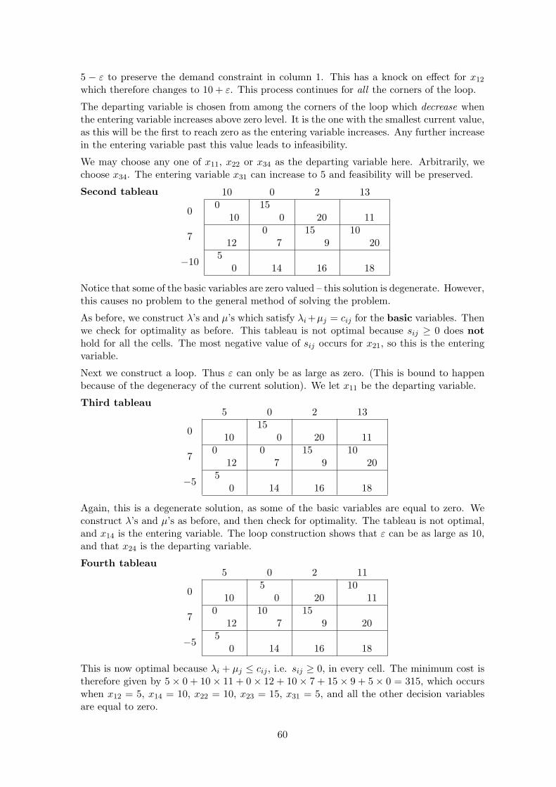
5 − ε to preserve the demand constraint in column 1. This has a knock on effect for x12

which therefore changes to 10 + ε. This process continues for all the corners of the loop.

The departing variable is chosen from among the corners of the loop which decrease whenthe entering variable increases above zero level. It is the one with the smallest current value,as this will be the first to reach zero as the entering variable increases. Any further increasein the entering variable past this value leads to infeasibility.

We may choose any one of x11, x22 or x34 as the departing variable here. Arbitrarily, wechoose x34. The entering variable x31 can increase to 5 and feasibility will be preserved.

Second tableau 10 0 2 13

00

1015

0 20 11

712

07

159

1020

−105

0 14 16 18

Notice that some of the basic variables are zero valued – this solution is degenerate. However,this causes no problem to the general method of solving the problem.

As before, we construct λ’s and µ’s which satisfy λi +µj = cij for the basic variables. Thenwe check for optimality as before. This tableau is not optimal because sij ≥ 0 does nothold for all the cells. The most negative value of sij occurs for x21, so this is the enteringvariable.

Next we construct a loop. Thus ε can only be as large as zero. (This is bound to happenbecause of the degeneracy of the current solution). We let x11 be the departing variable.

Third tableau5 0 2 13

010

150 20 11

70

120

715

910

20

−55

0 14 16 18

Again, this is a degenerate solution, as some of the basic variables are equal to zero. Weconstruct λ’s and µ’s as before, and then check for optimality. The tableau is not optimal,and x14 is the entering variable. The loop construction shows that ε can be as large as 10,and that x24 is the departing variable.

Fourth tableau5 0 2 11

010

50 20

1011

70

1210

715

9 20

−55

0 14 16 18

This is now optimal because λi + µj ≤ cij , i.e. sij ≥ 0, in every cell. The minimum cost istherefore given by 5 × 0 + 10 × 11 + 0 × 12 + 10 × 7 + 15 × 9 + 5 × 0 = 315, which occurswhen x12 = 5, x14 = 10, x22 = 10, x23 = 15, x31 = 5, and all the other decision variablesare equal to zero.

60

4.2.1 Example

This example emphasizes the connection between the transportation algorithm and theprimal-dual linear programming problems which underlie the method.

Three factories F1, F2, F3 produce 15000, 25000 and 15000 units respectively of a commod-ity. Three warehouses W1, W2, W3 require 20000, 19000 and 16000 units respectively.

The cost of transporting from Fi to Wj is £cij per unit, where c11 = 12, c12 = 7, c13 = 10,c21 = 10, c22 = 8, c23 = 6, c31 = 9, c32 = 15, c33 = 8.

If xij thousand units are transported from Fi to Wj , the total cost £1000z is given by

z = 12x11 + 7x12 + 10x13 + 10x21 + 8x22 + 6x23 + 9x31 + 15x32 + 8x33

which must be minimized subject to the constraints

x11 + x12 + x13 = 15x21 + x22 + x23 = 25

x31 + x32 + x33 = 15x11 + x21 + x31 = 20

x12 + x22 + x32 = 19x13 + x23 + x33 = 16

where xij ≥ 0 for i, j = 1, 2, 3.

By asymmetric duality, the dual of this problem is :

Maximize w = 15λ1 + 25λ2 + 15λ3 + 20µ1 + 19µ2 + 16µ3

subject to

λ1 + µ1 ≤ 12 i.e. λ1 + µ1 + s11 = 12λ1 + µ2 ≤ 7 i.e. λ1 + µ2 + s12 = 7

λ1 + µ3 ≤ 10 i.e. λ1 + µ3 + s13 = 10λ2 + µ1 ≤ 10 i.e. λ2 + µ1 + s21 = 10λ2 + µ2 ≤ 8 i.e. λ2 + µ2 + s22 = 8λ2 + µ3 ≤ 6 i.e. λ2 + µ3 + s23 = 6λ3 + µ1 ≤ 9 i.e. λ3 + µ1 + s31 = 9

λ3 + µ2 ≤ 15 i.e. λ3 + µ2 + s32 = 15λ3 + µ3 ≤ 8 i.e. λ3 + µ3 + s33 = 8

where sij ≥ 0 for i, j = 1, 2, 3 but λi, µj are unrestricted in sign.

Complementary slackness tells us that xijsij = 0 for all i and j.

12 7 10

10 8 6

9 15 8

12 7 10

10 8 6

9 15 8

61

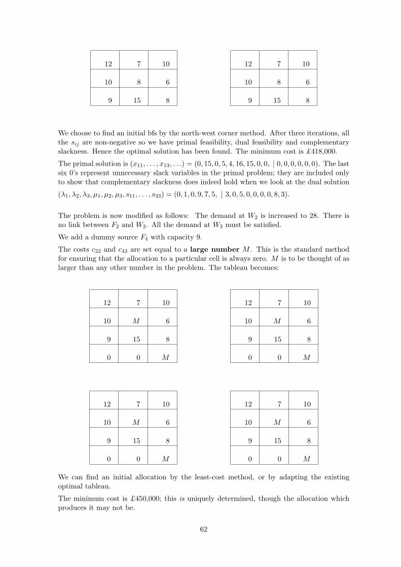
12 7 10

10 8 6

9 15 8

12 7 10

10 8 6

9 15 8

We choose to find an initial bfs by the north-west corner method. After three iterations, allthe sij are non-negative so we have primal feasibility, dual feasibility and complementaryslackness. Hence the optimal solution has been found. The minimum cost is £418,000.

The primal solution is (x11, . . . , x13, . . .) = (0, 15, 0, 5, 4, 16, 15, 0, 0, | 0, 0, 0, 0, 0, 0). The lastsix 0’s represent unnecessary slack variables in the primal problem; they are included onlyto show that complementary slackness does indeed hold when we look at the dual solution

(λ1, λ2, λ3, µ1, µ2, µ3, s11, . . . , s33) = (0, 1, 0, 9, 7, 5, | 3, 0, 5, 0, 0, 0, 0, 8, 3).

The problem is now modified as follows: The demand at W2 is increased to 28. There isno link between F2 and W2. All the demand at W3 must be satisfied.

We add a dummy source F4 with capacity 9.

The costs c22 and c43 are set equal to a large number M . This is the standard methodfor ensuring that the allocation to a particular cell is always zero. M is to be thought of aslarger than any other number in the problem. The tableau becomes:

12 7 10

10 M 6

9 15 8

0 0 M

12 7 10

10 M 6

9 15 8

0 0 M

12 7 10

10 M 6

9 15 8

0 0 M

12 7 10

10 M 6

9 15 8

0 0 M

We can find an initial allocation by the least-cost method, or by adapting the existingoptimal tableau.

The minimum cost is £450,000; this is uniquely determined, though the allocation whichproduces it may not be.

62

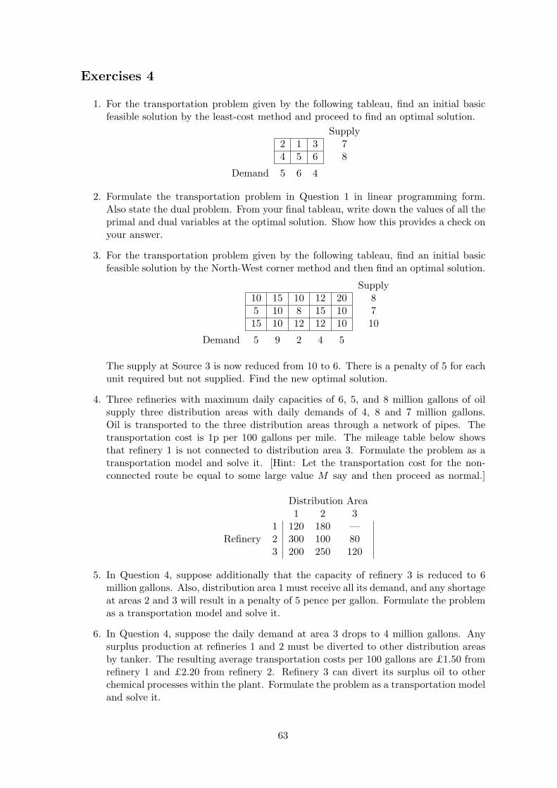
Exercises 4

1. For the transportation problem given by the following tableau, find an initial basicfeasible solution by the least-cost method and proceed to find an optimal solution.

Supply2 1 3 74 5 6 8

Demand 5 6 4

2. Formulate the transportation problem in Question 1 in linear programming form.Also state the dual problem. From your final tableau, write down the values of all theprimal and dual variables at the optimal solution. Show how this provides a check onyour answer.

3. For the transportation problem given by the following tableau, find an initial basicfeasible solution by the North-West corner method and then find an optimal solution.

Supply10 15 10 12 20 85 10 8 15 10 715 10 12 12 10 10

Demand 5 9 2 4 5

The supply at Source 3 is now reduced from 10 to 6. There is a penalty of 5 for eachunit required but not supplied. Find the new optimal solution.

4. Three refineries with maximum daily capacities of 6, 5, and 8 million gallons of oilsupply three distribution areas with daily demands of 4, 8 and 7 million gallons.Oil is transported to the three distribution areas through a network of pipes. Thetransportation cost is 1p per 100 gallons per mile. The mileage table below showsthat refinery 1 is not connected to distribution area 3. Formulate the problem as atransportation model and solve it. [Hint: Let the transportation cost for the non-connected route be equal to some large value M say and then proceed as normal.]

Distribution Area1 2 3

1 120 180 —Refinery 2 300 100 80

3 200 250 120

5. In Question 4, suppose additionally that the capacity of refinery 3 is reduced to 6million gallons. Also, distribution area 1 must receive all its demand, and any shortageat areas 2 and 3 will result in a penalty of 5 pence per gallon. Formulate the problemas a transportation model and solve it.

6. In Question 4, suppose the daily demand at area 3 drops to 4 million gallons. Anysurplus production at refineries 1 and 2 must be diverted to other distribution areasby tanker. The resulting average transportation costs per 100 gallons are £1.50 fromrefinery 1 and £2.20 from refinery 2. Refinery 3 can divert its surplus oil to otherchemical processes within the plant. Formulate the problem as a transportation modeland solve it.

63

Chapter 5

Non-linear optimization

5.1 Local and global optima

Let f be a real-valued function defined on a domain S ⊂ Rn, so f is applied to a vectorx = (x1, . . . , xn) ∈ S to give a real number f(x) as the result.

A vector x∗ ∈ S is a global maximizer of f(x) over S if f(x*) ≥ f(x) for all x ∈ S.

f(x*) is then the global maximum value of f(x) over S.

x∗ is a strong global maximizer of f(x) over S if f(x*) > f(x) for all x ∈ S other than x∗.

Replacing ‘≥’ or ‘>’ by ‘≤’ or ‘<’ gives the definitions for a (strong) global minimizer.

x* is a local maximizer of f(x) over S if there exists ε > 0 such that f(x*) ≥ f(x) wheneverx ∈ S and |x − x*| < ε. That is, f(x*) ≥ f(x) for all x ∈ S sufficiently close to x*.

Then f(x*) is a local maximum value of f(x). A local minimum is defined analogously.

An optimum or extremum is either a maximum or a minimum.

A global optimum is a local optimum, but a local optimum may not be a global optimum.

Recall that if f(x) is a differentiable function of one real variable x, local maxima andminima at interior points of the domain occur when f ′(x) = 0. The second derivative f ′′(x)is used to determine the nature of the optimum.

For functions of more than one real variable, the corresponding methods involve a vector offirst derivatives and a matrix of second derivatives, as follows:

The gradient vector of a differentiable function f(x) is ∇f(x) =

∂f(x)∂x1...

∂f(x)∂xn

.

A critical point of f(x) is a point at which ∇f(x) = 0.

The Hessian matrix of a twice-differentiable function f(x) is the symmetric n× n matrix

H(f(x)) =

∂2f(x)∂x2

1

∂2f(x)∂x1∂x2

· · · ∂2f(x)∂x1∂xn

∂2f(x)∂x2∂x1

∂2f(x)∂x2

2· · · ∂2f(x)

∂x2∂xn

......

. . ....

∂2f(x)∂xn∂x1

∂2f(x)∂xn∂x2

· · · ∂2f(x)∂x2

n

.

64

5.1.1 Examples

1. f(x, y, z) = 4x − 2y + z

2. f(x, y) = −2x2 + 6xy + y2

3. f(x, y, z) = e2xy +ln 2z

y

Now let f be a twice-differentiable real-valued function defined on a set S ⊂ Rn.

Let a = (a1, . . . , an) be in S and let u = (u1, . . . , un) be such that, for some c > 0, a+ru ∈ Sfor all r ∈ [0, c]. Such a vector u is called a feasible direction at a.

Let x = a + ru, so xi = ai + rui for i = 1, . . . , n. For 0 ≤ r ≤ c, define g(r) to be f(x).

By the Chain Rule, g′(r) =dg(r)dr

=df(x)dr

=n∑

i=1

∂f(x)∂xi

dxi

dr=

n∑i=1

ui∂f(x)∂xi

= ut∇f(x).

Hence g ′(0) = ut∇f(a).

When u is a unit vector, ut∇f(a) is called the directional derivative of f at a in thedirection u. It measures the rate of increase of f as we move from a in the direction u.

Also g′′(r) =ddr

(n∑

i=1

ui∂f(x)∂xi

)=

n∑i=1

ui

n∑j=1

∂2f(x)∂xi∂xj

dxj

dr=

n∑i,j=1

ui∂2f(x)∂xi∂xj

uj = utH(f(x))u,

so g ′′(0) = utH(f(a))u. Thus we have:

65

Proposition 5.1 If g(r) = f(a + ru) then g′(0) = ut∇f(a) and g′′(0) = utH(f(a))u.

Proposition 5.2 (First order necessary condition for a local optimum.)Let f(x) be a differentiable function on S ⊂ Rn. If f(x) attains a local maximum or minimumvalue over S at an interior point x∗ ∈ S then ∇f(x∗) = 0.

Proof

As x∗ is an interior point of S, we can move from x∗ in any direction u and still be in S.

If x∗ is a local maximizer, f(x) must be non-increasing in every direction moving away fromx∗ so ut∇f(x∗) ≤ 0 and (−u)t∇f(x∗) ≤ 0. Hence ut∇f(x∗) = 0 for all u ∈ Rn.

Taking u = ei (the vector with ith entry 1 and all other entries 0) shows that the ithcomponent of ∇f(x∗) is 0 for i = 1, . . . , n. Hence ∇f(x∗) = 0.

If x∗ is a local minimizer, the same reasoning applies with ‘decrease’ replaced by ‘increase’and ‘≤’ by ‘≥’.

This condition is not sufficient for a maximum or minimum, as ∇f(x) = 0 also holds at asaddle point, i.e. a critical point where f(x) is locally neither minimum nor maximum.

5.2 Quadratic forms

Recall that if A is a square matrix, the function xtAx is called a quadratic form. Anyexpression consisting entirely of second-order terms can be written in this form. We canalways choose A to be symmetric.

For example, x12 − 8x1x2 + 5x2

2 = xtAx, where x =(

x1

x2

)and A =

(1 −4

−4 5

).

Similarly 2x2 + y2 − z2 + 4xy − 6yz =(

x y z) 2 2 0

2 1 −30 −3 −1

xyz

.

A real square matrix A, and equivalently the quadratic form xtAx, is defined to be

positive definite if xtAx > 0 ∀ x 6= 0, positive semi-definite if xtAx ≥ 0 ∀ x,

negative definite if xtAx < 0 ∀ x 6= 0, negative semi-definite if xtAx ≤ 0 ∀ x,

indefinite if none of the above is true. (Note that ‘semi-definite’ includes ‘definite’.)

When x ∈ R2, we can visualise these definitions graphically; e.g. if A is positive definite,the surface z = xtAx lies wholly above the (x, y) plane and meets it only at (0, 0, 0).

By orthogonally diagonalizing the symmetric matrix, any quadratic form can be expressedas λ1y1

2 + · · · + λnyn2 where λ1, . . . , λn are the eigenvalues of the matrix. Using this we

showed in Level 1 Linear Algebra that a real symmetric matrix is positive definite if andonly if all its eigenvalues are positive, and negative definite if and only if all its eigenvaluesare negative.

The determinant of a square matrix is the product of the eigenvalues, so if a real symmetricmatrix is positive definite then its determinant is strictly positive.

The converse of this is not true, but we can say that if a real symmetric matrix A is eitherpositive or negative definite then it is non-singular. If A is semi-definite but not definite,xtAx = 0 for some x 6= 0, hence some λi = 0 so A is singular.

66

The kth order principal minors of an n×n matrix A are the determinants of all the k×kmatrices that can be formed using k rows and the corresponding k columns of A.

The kth leading principal minor of A is the determinant of the k × k matrix formedfrom the first k rows and the first k columns of A.

Thus the first leading principal minor is just the top left entry and the nth one is det(A).

For example,

4 2 −32 −1 0

−3 0 3

has principal minors 4,−1, 3 (first order), −8, 3,−3 (sec-

ond order), −15 (third order). The leading ones are 4,−8,−15.

Proposition 5.3 A real symmetric matrix A is positive definite if and only if all its leadingprincipal minors are strictly positive.

Proof

(⇐) Let Mj be the submatrix of A consisting of the first j rows and the first j columns.

We can write A =(

Mj Qj

Rj Sj

)where Qj , Rj , Sj are matrices of appropriate sizes (0 × 0

when j = n).

Suppose all leading principal minors of A are positive, so det(M1), . . . , det(Mn) are all > 0.

For j = 1, . . . , n, let uj be the vector in Rj with jth entry 1 and all other entries (if any) 0

and let pj =

p1j...

pjj

satisfy the linear system of equations Mjpj = uj .

By Cramer’s rule, pjj =det(Mj−1)det(Mj)

which is greater than 0.

Let P be the upper triangular matrix with entries pij for i ≤ j and 0 for i > j.

The jth column of P is pj =(

pj

0

).

Thus column j of AP is(

Mj Qj

Rj Sj

)(pj

0

)=(

Mjpj

Rjpj

)=(

uj

Rjpj

).

Hence AP is lower-triangular, with all the entries on its main diagonal equal to 1.

Let C = PtAP. C is a product of two lower-triangular matrices, so is itself lower-triangular.But Ct = PtAtP = PtAP as A is symmetric, so C is symmetric. Hence C is a diagonalmatrix, and its diagonal entries are p11, . . . , pnn which we have seen are all positive.

Let x = Py. Then xtAx = ytCy =n∑

j=1

pjjyj2 > 0 for all y 6= 0.

P is non-singular, so y 6= 0 iff x 6= 0. Hence xtAx > 0 for all x 6= 0, so A is positive definite.

(⇒) Suppose A is positive definite.

Let y be any non-zero vector in Rj and let x =(

y0

)∈ Rn.

Then xtAx = (yt | 0)(

Mj Qj

Rj Sj

)(y0

)= (yt | 0)

(MjyRjy

)= ytMjy.

67

Since x 6= 0 and A is positive definite, xtAx > 0, so ytMjy > 0 for all y 6= 0.

Hence Mj is positive definite, and thus det(Mj) > 0 for j = 1, . . . , n.

Note that A is positive definite if and only if −A is negative definite. The leading principalminors of −A are then alternately negative and positive.

The results can be further extended to semi-definite matrices. The following table gives nec-essary and sufficient conditions for a real symmetric matrix A, and the associated quadraticform xtAx, to be positive / negative (semi-) definite. Either the eigenvalues condition orthe principal minors condition may be used. The latter is generally easier.

Symmetric matrix Definition Eigenvalues Principal MinorsPositive definite xtAx > 0 ∀x 6= 0 All > 0 Leading ones all positive.

Positive semi-definite xtAx ≥ 0 ∀x All ≥ 0 All non-negative.Negative definite xtAx < 0 ∀x 6= 0 All < 0 jth l.p.m. has sign of (−1)j

Negative semi-definite xtAx ≤ 0 ∀x All ≤ 0 Those of −A non-negativeIndefinite None of above Some +, some − None of the above

5.2.1 Examples

1. A =(

−3 22 −4

).

2. B =(

3 −6−6 12

).

3. C =

1 0 −20 3 −1

−2 −1 5

.

68

4. D =

4 2 −32 −1 0

−3 0 3

.

Proposition 5.4 (Second order sufficient conditions for local optima.)Let f(x) be a twice-differentiable function on S ⊂ Rn. Suppose ∇f(x∗) = 0.

(i) If H(f(x∗)) is positive definite then x∗ is a strong local minimizer of f(x).

(ii) If H(f(x∗)) is negative definite then x∗ is a strong local maximizer of f(x).

(iii) If H(f(x∗)) is indefinite and non-singular then f(x) has a saddle-point at x∗.

Proof of (i)

Let u be any feasible direction at x∗. Let g(r) = f(x∗ + ru), so g(0) = f(x∗).

By Proposition 5.1, g′(0) = ut∇f(x∗) and g

′′(0) = utH(f(x∗))u .

Thus if ∇f(x∗) = 0 then g′(0) = 0.

If also H(f(x∗)) is positive definite, i.e. utH(f(x∗))u > 0 for all u 6= 0, then g′′(0) > 0

Hence r = 0 is a strong local minimizer of g(r), so g(0) < g(r) for all r close to 0.

Equivalently, f(x∗) < f(x∗ + ru) for small enough r and all feasible directions u. Thus x∗ isa strong local minimizer of f(x) over S.

69

5.2.2 Examples

(i) f(x) = xyz − x2 − y2 − z2.

(ii) f(x) = 5x + 4y + 2z − 2x2 − 3y2 − 5z2 − 2xy − 6xz − 4yz.

70

5.3 Convex and concave functions

A twice-differentiable function f defined on an interval S ⊂ R is convex on S if f′′(x) ≥

0 for all x ∈ S, and concave on S if f′′(x) ≤ 0 for all x ∈ S. (Note: this definition of

convexity applies only to functions of one variable. The general definition is given below.)

Examples of convex functions of one variable x are: x2, x4, ex, cosh x.

Examples of concave functions of one variable x are:√

x, lnx, e−x, arctanx.

Geometrically, if S is the interval [a, b], a convex function f lies below (or on) the straightline joining A (a, f(a)) and B (b, f(b)).

If c ∈ S, then c = (1 − r)a + rb for some r with 0 ≤ r ≤ 1. Then f(c) = f((1 − r)a + rb),while the point on the straight line AB at which x = c has y-coordinate (1− r)f(a) + rf(b).Thus f((1 − r)a + rb) ≤ (1 − r)f(a) + rf(b) for all r ∈ [0, 1].

For functions of any number of variables, the definitions are as follows:

Let f be a real-valued function defined on a convex subset S of Rn.

f is a convex function on S if for any x, y ∈ S,

f((1 − r)x + ry) ≤ (1 − r)f(x) + rf(y) for all r ∈ [0, 1].

f is a concave function if for any x, y ∈ S,

f((1 − r)x + ry) ≥ (1 − r)f(x) + rf(y) for all r ∈ [0, 1].

f is a strictly{ convex

concave

}function on S if for any x, y ∈ S with x 6= y,

f((1 − r)x + ry){<

>

}(1 − r)f(x) + rf(y) for all r ∈ (0, 1).

Clearly f is concave if and only if −f is convex.

If f is a convex function of one or two variables, its graph lies below (or on) the straight linejoining any two points on it, so the region above it is a convex set.

If f is a concave function of one or two variables, its graph lies above (or on) the straightline joining any two points on it, so the region below it is a convex set.

• Any linear function is both convex and concave, but not strictly so.

• A positive multiple of a convex / concave function is itself convex / concave. Forexample, x2 is convex on R, so ax2 is convex on R for any a > 0.

• A sum of convex / concave functions is itself convex / concave. For example, x2, y4

and z6 are each convex, so x2 + y4 + z6 is convex on R3.

It may not be clear from the definitions whether a function of several variables is convex,concave or neither. For functions of more than one variable it is not enough just to considerthe second derivatives. We therefore derive criteria which are easier to use.

Proposition 5.5 A twice-differentiable function f defined on a convex set S ⊂ Rn is

(i) convex on S if and only if, at each x ∈ S, H(f(x)) is positive semi-definite;

(ii) concave on S if and only if, at each x ∈ S, H(f(x)) is negative semi-definite;

71

(iii) strictly convex on S if, at each x ∈ S, H(f(x)) is positive definite;

(iv) strictly concave on S if, at each x ∈ S, H(f(x)) is negative definite.

(Note that ‘semi-definite’ includes ‘definite’.)

Proof: We prove the ‘if’ part of (i).

Let x and y be in S and let u = y − x.

For 0 ≤ r ≤ 1, let z = (1 − r)x + ry = x + ru. As S is a convex set, z ∈ S.

Let g(r) = f(z), so g(0) = f(x) and g(1) = f(y).

As in the proof of Proposition 5.1, g′′(r) = utH(f(z))u.

If H(f(x)) is positive semi-definite for all x ∈ S then utH(f(z))u ≥ 0.

Thus g′′(r) ≥ 0 for 0 ≤ r ≤ 1 so g is a convex function on [0, 1].

f((1 − r)x + ry) = f(z) = g(r) = g((1 − r)(0) + r(1)) ≤ (1 − r)g(0) + rg(1) (as g is convex)

= (1 − r)f(x) + rf(y). Thus f is convex on S.

Proposition 5.6 Let f be a{ convex

concave

}function on a convex set S ⊂ Rn. If there is a

point x∗ ∈ S for which ∇f(x∗) = 0 then x∗{

minimizes

maximizes

}f(x) globally over S.

Proof (Convex case)

Suppose ∇f(x∗) = 0. Let u be any vector such that y = x∗ + u ∈ S.

x∗ + ru = (1 − r)x∗ + ry ∈ S for all r ∈ [0, 1], as S is convex.

Let g(r) = f(x∗ + ru), so g(0) = f(x∗) and g(1) = f(y).

Assume f is convex, so f((1 − r)x∗ + ry) ≤ (1 − r)f(x∗) + rf(y).

Thus g(r) ≤ (1 − r)g(0) + rg(1), so if r > 0 theng(r) − g(0)

r≤ g(1) − g(0).

As r → 0, the left hand side tends to g ′(0). But g ′(0) = ut∇f(x∗) = 0 since ∇f(x∗) = 0.

Hence 0 ≤ g(1) − g(0) so g(1) ≥ g(0), i.e. f(y) ≥ f(x∗), for all y ∈ S.

Thus x∗ minimizes f(x) globally over S.

It can also be shown that every local{

minimizermaximizer

}of a

{ convexconcave

}function is global, even

if it does not occur at a critical point.

For example, a concave function might have a local maximizer which is not at a criticalpoint, on the boundary of its domain. This would have to be a global maximizer.

72

5.3.1 Examples

(i) f(x, y) = 3x2 + 4y2 − 5xy + 2x − 3y.

(ii) f(x, y, z) = ln(xy) − y

zwhere x, y, z > 0. (iii) Let f(x, y) = x4 + y4.

73

Exercises 5

1. Express each of the following in the form xtAx, where A is a symmetric matrix.

(a) 4x2 + 3y2, (b) −3x2 + 4xy − 6y2, (c) x2 + y2 + z2,

(d) 3x2 + 2y2 + z2 + 4xy + 4yz, (e) 3x2 + 5y2 + 2z2 + 4xy − 2xz − 4yz.

Determine whether each is positive or negative definite or semi-definite or indefinite.

2. Using the Hessian matrices where appropriate, find and classify the local optima of

(a) 2x2 − ln |2x|, (b) 3x2 + 4xy − 8y, (c) x3 + 4xy − 6y2,

(d) x2 + 3y2 + 4z2 − 2xy − 2xz + 3yz − y, (e) x3 + y3 + z3 − 9xy − 9xz + 27x.

3. Determine whether each of the following is convex, concave or neither on S.

(a) f(x) =1x

, S = (0,∞), (b) f(x) = xα, 0 ≤ α ≤ 1, S = (0,∞),

(c) f(x, y) = x3 + 3xy + y2, S = R2, (d) f(x, y, z) = −x2 − y2 − 2z2 +12xy, S = R3.

4. Let f(x, y, z) = x2 − y2 − xy − x3

Find S, the largest convex subset of R2 on which f is a concave function.

Find, with justification, the global maximum value of f over S.

5. Find the values of x, y and z which minimize f(x, y, z) = x2+2y2+3z2+2xy+2xz−4yover R3. Justify that the point you find is a global minimizer.

6. The function f is quasi-convex on Rn if for every real number a, the set S = {x ∈ Rn :f(x) ≤ a} is a convex set. Prove that any convex function on Rn is quasi-convex.

74

Chapter 6

Constrained optimization

6.1 Lagrange multipliers

Consider the constrained optimization problem:

maximize or minimize f(x) = f(x1, . . . , xn)

subject to gj(x) = bj for j = 1, . . . , m,

where x ∈ S ⊂ Rn.

Here, f and g1, . . . , gm are functions from Rn to R, and m < n.

Let g(x) = (g1(x) · · · gm(x))t, b = (b1 · · · bm)t, so the constraints can be expressed asg(x) = b.

Let λ = (λ1 · · · λm)t. The Lagrangean function for the optimization problem is

L(x1, . . . , xn, λ1, . . . , λm) = f(x1, . . . , xn) +m∑

j=1λj(bj− gj(x1, . . . , xn))

which can be written as L(x, λ) = f(x) + λt(b − g(x)).

λ1, . . . , λm are called Lagrange multipliers. There is one for each constraint.

75

6.1.1 Example

Suppose we have to maximize f(x1, x2, x3) = x12 + 2x2x3 subject to the constraints

x1 + x2 = 5, x12 − x2

2 = 4 and x1x2x3 = 7.

Proposition 6.1 (Lagrange sufficiency theorem)(i) If there exist λ∗ ∈ Rm and x∗ ∈ S such that L(x∗, λ∗) ≥ L(x, λ∗) for all x ∈ S, andg(x∗) = b, then x∗ maximizes f(x) over S subject to g(x) = b.

(ii) If there exist λ∗ ∈ Rm and x∗ ∈ S such that L(x∗, λ∗) ≤ L(x, λ∗) for all x ∈ S, andg(x∗) = b, then x∗ minimizes f(x) over S subject to g(x) = b.

Proof of (i) [the proof of (ii) is similar]

Assume L(x∗, λ∗) ≥ L(x, λ∗) for all x ∈ S,

so f(x∗) + (λ∗)t(b − g(x∗)) ≥ f(x) + (λ∗)t(b − g(x)) for all x ∈ S.

By assumption g(x∗) = b, so b − g(x∗) = 0.

Hence f(x∗) ≥ f(x) for all x ∈ S with g(x) = b,

so x∗ maximizes f(x) over S subject to g(x) = b.

Now suppose f and each gi are differentiable and that a constrained optimum of f(x) occursat an interior point x* in S.

If f and the gi are fixed, we can treat x∗ as a function of b: call it x∗(b).

Let v(b) = f(x∗(b)) and let h(x) = f(x) − v(g(x)).

Then where the constraints hold, h(x) = f(x) − v(b). In particular, for any b, h(x∗(b)) =f(x∗(b)) − v(b) = 0.

For each x, v(g(x)) is the optimal value of f(y) subject to g(y) = g(x). As x is feasible forthis problem, v(g(x)) ≥ f(x), i.e. h(x) ≤ 0, for all x ∈ S if the problem is a maximization,and v(g(x)) ≤ f(x), i.e. h(x) ≥ 0, for all x ∈ S if the problem is a minimization.

Thus x∗ is an interior point of S at which h(x) is either maximized or minimized, so∇h(x∗) = 0.

Now ∇h(x) = ∇f(x) −∇v(g(x)).

76

By the chain rule,∂h(x)∂xi

=∂f(x)∂xi

−m∑

j=1

∂v(g(x))∂gj(x)

∂gj(x)∂xi

=∂f(x)∂xi

−m∑

j=1

λj(x)∂gj(x)

∂xi

where λj(x) =∂v(g(x))∂gj(x)

.

Let λj∗ = λj(x∗). As ∇h(x∗) = 0, we have

∂f∂xi

(x∗) =m∑

j=1

λj∗∂gj

∂xi(x∗),

so ∇f(x∗) =m∑

j=1λj

∗∇gj(x∗). Equivalently, ∇xL(x∗, λ∗) = 0, where ∇x denotes the gradient

vector with respect to (x1, . . . , xn).

If the m vectors ∇gj(x∗) form a linearly independent set then ∇f(x∗) can be expressed as alinear combination of them in only one way, so the multipliers λj

∗ are uniquely determined.Hence we have:

Proposition 6.2 (Lagrange necessity theorem)Let x∗ be an interior point of a set S which is a local maximizer or minimizer of f(x) overS subject to g(x) = b. Suppose the set {∇g1(x∗), . . . , ∇gm(x∗)} is linearly independent.Let L(x, λ) = f(x) + λt(b − g(x)).

Then there is a unique vector λ∗ ∈ Rm such that x∗, λ∗ satisfy ∇xL(x∗, λ∗) = 0.

6.1.2 Examples

(i) Maximise f(x, y) = xy over R2 subject to g(x, y) = x + y = 8.

(ii) Find the optimal value(s) of the function f(x, y, z) = 4x1/4y1/4z1/4 over R3+ subject to

the constraints x + y = 3, y + z = 3.

77

(iii) Minimize f(x, y, z) = x2 + y2 + z2 over R3, subject to x + 2y + z = 1 and 2x−y−3z = 4.

Let L(x, y, z, λ1, λ2) = x2 + y2 + z2 + λ1(1 − x − 2y − z) + λ2(4 − 2x + y + 3z).

Sensitivity analysis

In the proof of the Lagrange necessity theorem, we defined λj(x) to be∂v(g(x))∂gj(x)

.

78

Thus λj∗ =

∂v(g(x∗))∂gj(x∗)

=∂v(b)∂bj

,

i.e. the optimal value of the Lagrange multiplier for the jth constraint is equal to the rateof change in the maximal value of the objective function as the jth constraint is relaxed.

If an increase δbj in the right-hand side of a constraint yields an increase δV in the optimalvalue of f(x) then δV ≈ λj

∗ δbj .

If the constraints arise because of limits on some resources, then λj∗ is called the shadow

price of the jth resource.

If all the bj can vary, δV ≈m∑

j=1

∂V

∂bjδbj =

m∑j=1

λj∗ δbj . Thus we have:

Proposition 6.3 Suppose x∗ optimizes f(x) over S subject to gj(x) = bj for j = 1, . . . , m.Let λ1

∗, . . . , λm∗ be the values of the Lagrange multipliers at the optimal point.

If each bj is increased by a small amount δbj, then the increase in the optimal value of f(x)

is approximatelym∑

j=1

λj∗ δbj.

In Example 6.1.2 (ii), f(x∗) = 4√

2, b1 = b2 = 3, λ1∗ = λ2

∗ =1√2.

If b1 and b2 are slightly increased, say to 3.1 and 3.2 respectively, we would expect the

constrained maximum to be increased by about 0.3 × 1√2, to approximately 5.87.

6.2 Constrained optimization of quadratic forms

Let A be a symmetric real matrix. In this section we seek to optimize the quadratic formq(x) = xtAx subject to the non-linear constraint | x | = 1, which can also be written asxtx = 1 or x1

2 + · · · + xn2 = 1.

First we note that ∇(xtx) = ∇(x12 + · · · + xn

2) = (2x1, . . . , 2xn) = 2x

and if A is symmetric, ∇(xtAx) = ∇

(n∑

i,j=1aijxixj

). The partial derivative of this with

respect to xi is 2aiixi + 2∑j 6=i

aijxj = 2n∑

j=1aijxj , so ∇(xtAx) = 2Ax when A is symmetric.

Proposition 6.4 Let A be a symmetric real matrix and let q(x) = xtAx.

The minimum value of q(x) subject to | x | = 1 is equal to the smallest eigenvalue of A,and occurs when x is a corresponding unit eigenvector.

The maximum value of q(x) subject to | x | = 1 is equal to the largest eigenvalue of A, andoccurs when x is a corresponding unit eigenvector.

Proof

The constraint is xtx = 1, i.e. 1 − xtx = 0.

The Lagrangean function is L(x, λ) = xtAx + λ(1 − xtx).

For q(x) to be optimal subject to the constraint, ∇xL(x, λ) = 0.

79

Hence 2Ax − 2λx = 0, giving Ax = λx. Also xtx = 1.

Thus λ is an eigenvalue of A, with eigenvector x such that xtx = 1, i.e. x is a unit vector.

So the necessary condition for an optimum of q(x) is satisfied when x is such an eigenvectorof A. Then q(x) = xtAx = xt(λx) = λ(xtx) = λ.

The feasible set is compact, so by Weierstrass’s Theorem the minimum and maximum exist.Thus they must be among the values we have found, which are in R since the eigenvaluesof a symmetric real matrix are real. The result follows.

6.2.1 Example

Find the maximum and minimum values of q = x2+z2+4xz−6yz subject to x2+y2+z2 = 1.

6.2.2 Example

A council plans to repair x hundred miles of roads and improve y hundred acres of parks.Budget restrictions lead to the constraint 4x2 + 9y2 = 36. The benefit obtained from thepossible work schedules is U = xy. Find the schedule that maximizes U .

80

Exercises 6

1. A firm has to minimize its cost function C(x, y) = rx + wy subject to the constraintx1/2y1/4 = 8. Find the minimum cost in terms of the constants r and w.

2. Find (i) the minimum value of x2 + y2 subject to the constraint 2x − 3y = 4,

(ii) the maximum value of x2y2 subject to the constraint 2x2 + y2 = 3,

Interpret your answers graphically.

3. f(x, y, z) = x1/3y1/3z1/3 where x > 0, y > 0, z > 0.

Maximize f(x, y, z) subject to the constraints x + y = 3 and y + z = 3.

4. The total profit £z thousand which a company makes from producing and selling xthousand units of one commodity X and y thousand units of another commodity Yis given by z = 10 + 50x − 5x2 + 16y − y2.

(a) Find the maximum value of z if there are no constraints on x and y, explainingwhy the value you find is a maximum.

(b) Find the maximum value of z if the total cost of production is to be £12,000,given that each unit of X costs £4 to produce and each unit of Y costs £3.20.

(c) The company now increases the money available for production to £12,500. Usesensitivity analysis to estimate the new maximum profit.

5. A firm’s production function, using quantities x, y, z of three inputs, is defined byP (x, y, z) = x

12 ln y − z2, where x > 0, y > 0, z > 0.

Find the largest region of R3+ on which P is a concave function.

Maximize P (x, y, z) over this region subject to the constraints x + y − z = e4 and−x + 2y + z = 2e4.

6. A consumer’s satisfaction with three foods is measured by U(x1, x2, x3) = x1 +lnx2 +2x3, where x1 > 0, x2 > 0, x3 > 0 and xi is the number of units of food i consumed.

Foods 1, 2 and 3 cost £2,£1,£0 per unit and contain 0, 100 and 200 calories per unitrespectively.

The consumer wants to spend exactly £10 and consume 1000 calories.

Find the maximum value of U(x1, x2, x3). Justify that the value you have found is amaximum.

Using sensitivity analysis, estimate the increase in this maximum value if an extra £1may be spent and an extra 50 calories consumed.

7. Use Proposition 6.4 to find the maximum and minimum values of the followingquadratic forms subject to the constraint

∑xi

2 = 1. Also find the values of thevariables xi at which the optimal values are attained.

(a) q(x1, x2) = 5x12 + 5x2

2 − 4x1x2, (b) q(x1, x2) = 7x12 + 3x2

2 + 3x1x2,

(c) q(x1, x2, x3) = −2x12 − x2

2 + 4x1x2 + 4x2x3.

81

Sample Class test

1. A predator needs a daily intake of at least 10 units of food A, 12 units of food B and12 units of food C. These requirements are satisfied by feeding on two species of prey.

One animal of species 1 contains 5 units of A, 2 units of B amd 1 unit of C.

One animal of species 2 contains 1 unit of A, 2 units of B and 4 units of C.

To catch and digest each animal takes 3 units of energy for species 1 and 2 units ofenergy for species 2. The predator needs to minimise its daily expenditure of energy.

(a) If x1 animals of species 1 and x2 of species 2 are consumed in a day, formulatethe above information as a linear programming problem. [4]

(b) The feasible region for the problem is shown in the diagram:

0

2

4

6

8

10

12

2 4 6 8 10 12

From the graph, find how many of each speciesthe predator should eat to satisfy its daily re-quirements with the minimum expenditure ofenergy. State the optimal number of units ofenergy used. [4]

(c) Species 2 is becoming tougher, and to catch and digest one animal now requiresq units of energy. How large does q have to become before the optimal feedingplan changes? State how many of each species should be consumed per day whenq slightly exceeds this value. [4]

2. z = 3x1 + 2x2 + 5x3 is to be maximized subject to the constraints

x1 + 2x2 + x3 ≤ 4303x1 + + 2x3 ≤ 460x1 + 4x2 ≤ 420

where x1 ≥ 0, x2 ≥ 0, x3 ≥ 0.

(a) Write the constraints in standard form. [2]

(b) Using the simplex algorithm, show that the maximum value of z is 1350. [10]

(c) State the values of x1, x2 and x3 at which the maximum occurs. [2]

(d) Express z in terms of the variables which are non-basic in the final tableau.Hence explain why the solution is optimal. [4]

82

(e) B−1 is the 3× 3 matrix which pre-multiplies the middle three rows of the initialtableau to give those rows in the final tableau. Write down B−1 and B. [4]

(f) If the first constraint is changed to x1 + 2x2 + x3 ≤ k, find the range of valuesof k for which the same variables remain basic at the optimum. If k lies in thisrange, express the new optimal value of z in terms of k. [6]

3. Give definitions of the following:

(a) a non-negative vector in Rn, [2]

(b) a convex subset of Rn, [2]

(c) an extreme point of a convex set, [2]

(d) a bounded subset of Rn, [2]

(e) an algorithm of exponential complexity. [2]

[TOTAL MARKS: 50]

83

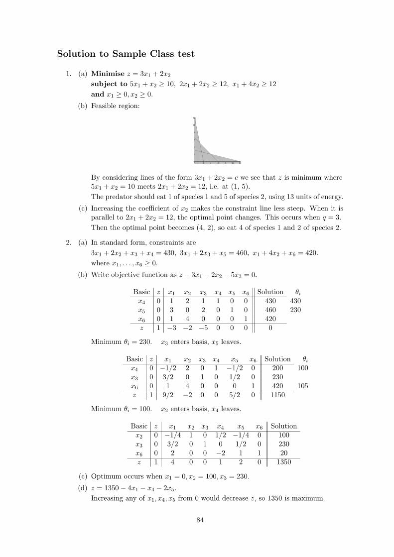
Solution to Sample Class test

1. (a) Minimise z = 3x1 + 2x2

subject to 5x1 + x2 ≥ 10, 2x1 + 2x2 ≥ 12, x1 + 4x2 ≥ 12and x1 ≥ 0, x2 ≥ 0.

(b) Feasible region:

0

2

4

6

8

10

12

2 4 6 8 10 12

By considering lines of the form 3x1 + 2x2 = c we see that z is minimum where5x1 + x2 = 10 meets 2x1 + 2x2 = 12, i.e. at (1, 5).The predator should eat 1 of species 1 and 5 of species 2, using 13 units of energy.

(c) Increasing the coefficient of x2 makes the constraint line less steep. When it isparallel to 2x1 + 2x2 = 12, the optimal point changes. This occurs when q = 3.Then the optimal point becomes (4, 2), so eat 4 of species 1 and 2 of species 2.

2. (a) In standard form, constraints are3x1 + 2x2 + x3 + x4 = 430, 3x1 + 2x3 + x5 = 460, x1 + 4x2 + x6 = 420.

where x1, . . . , x6 ≥ 0.

(b) Write objective function as z − 3x1 − 2x2 − 5x3 = 0.

Basic z x1 x2 x3 x4 x5 x6 Solution θi

x4 0 1 2 1 1 0 0 430 430x5 0 3 0 2 0 1 0 460 230x6 0 1 4 0 0 0 1 420z 1 −3 −2 −5 0 0 0 0

Minimum θi = 230. x3 enters basis, x5 leaves.

Basic z x1 x2 x3 x4 x5 x6 Solution θi

x4 0 −1/2 2 0 1 −1/2 0 200 100x3 0 3/2 0 1 0 1/2 0 230x6 0 1 4 0 0 0 1 420 105z 1 9/2 −2 0 0 5/2 0 1150

Minimum θi = 100. x2 enters basis, x4 leaves.

Basic z x1 x2 x3 x4 x5 x6 Solutionx2 0 −1/4 1 0 1/2 −1/4 0 100x3 0 3/2 0 1 0 1/2 0 230x6 0 2 0 0 −2 1 1 20z 1 4 0 0 1 2 0 1350

(c) Optimum occurs when x1 = 0, x2 = 100, x3 = 230.

(d) z = 1350 − 4x1 − x4 − 2x5.Increasing any of x1, x4, x5 from 0 would decrease z, so 1350 is maximum.

84

(e) B−1 =

1/2 −1/4 00 1/2 0

−2 1 1

. (under x4, x5, x6 in optimal tableau)

B =

2 1 00 2 04 0 1

. (under x2, x3, x6 in optimal tableau)

(f) If original solution column is b = (k 460 420)t, final solution column is

B−1b =(

k

2− 115 230 880 − 2k

)t

.

For this to be non-negative, k ≥ 230 and k ≤ 440.Then zmax = (1 2 0)b = k + 920.

85