matching in marriage market and labor market

Matching in Marriage Market and Labor Market

So Yoon Ahn

Submitted in partial fulfillment of the

requirements for the degree of

Doctor of Philosophy

in the Graduate School of Arts and Sciences

COLUMBIA UNIVERSITY

2018

ABSTRACT

Matching in Marriage Market and Labor Market

So Yoon Ahn

This dissertation examines how matching – in marriage markets and labor mar-

kets – can change under certain market circumstances and under different information

provisions.

The first two chapters analyze marriage market, with a particular focus on the im-

pacts of cross-border marriage in marriage markets. Given the severely male-biased sex

ratios in many Asian countries including China and India, demands for foreign brides

are expected to grow in the near future. In the first chapter, I theoretically investi-

gate the impacts of cross-border marriage on marital patterns and surplus division of

couples. I use a frictionless transferable utility matching framework to analyze how

cross-border marriage affects matching patterns and marital shares for couples.

In the second chapter, I test the model’s predictions, focusing on Taiwan (a wealthier

side with male biased sex ratios) and Vietnam (a poorer side with balanced sex ratios in

the marriage market). I find that cross-border marriages are predominantly made up of

Taiwanese men and Vietnamese women; Taiwanese men are selected from the middle

level of the socioeconomic status distribution, and Vietnamese women are positively

selected. Moreover, cross-border marriage significantly affects men and women who stay

in their own countries without engaging in cross-border marriage, by altering marriage

rate, matching partners, and intra-household allocations within the households. My

results suggest that changes in trade and immigration policies can have far-reaching

implications on marital outcomes and women’s bargaining power.

The third chapter investigates job and jobseeker matching in labor market. Specif-

ically, it explores whether inaccurate expectations of job seekers about their competi-

tiveness contribute to poor job matching in developing countries. We utilize the largest

online job portal in the Middle East and North Africa region to evaluate the effect of an

intervention providing information about own competitiveness to job applicants. Pro-

viding information about the relative fit of an applicant’s background for a particular

job causes job seekers to apply for jobs that are better matches given their background.

The effects of information are the largest among entry-level workers with higher levels

of education, who generally face the highest unemployment rates in the region. The

findings are consistent with the hypothesis that changes over time in demand for skills

in the job market may lead to inaccurate expectations that hinder labor market match-

ing. Improving the efficiency of online job search may be particularly welfare-enhancing

in the Middle East and North Africa region given that the young, highly-educated sub-

population that faces the greatest labor market hurdles also has the highest level of

internet connectedness.

Contents

List of Figures iii

List of Tables v

1 Matching Across Markets: Theory of Cross-Border Marriage 1

1.1 Introduction . . . . . . . . . . . . . . . . . . . . . . . . . . . . . . . . . 2

1.2 Country Background . . . . . . . . . . . . . . . . . . . . . . . . . . . . 6

1.3 Model . . . . . . . . . . . . . . . . . . . . . . . . . . . . . . . . . . . . 9

1.4 General Results . . . . . . . . . . . . . . . . . . . . . . . . . . . . . . . 10

1.5 Example: Taiwan and Vietnam . . . . . . . . . . . . . . . . . . . . . . 13

1.6 Conclusion . . . . . . . . . . . . . . . . . . . . . . . . . . . . . . . . . . 19

2 Matching Across Markets: Evidence of Cross-Border Marriage from

Taiwan and Vietnam 21

2.1 Introduction . . . . . . . . . . . . . . . . . . . . . . . . . . . . . . . . . 22

2.2 Data . . . . . . . . . . . . . . . . . . . . . . . . . . . . . . . . . . . . . 27

2.3 Empirical Evidence on the Selection of Cross-Border Couples . . . . . . 31

2.4 Impacts of Cost Increases in Taiwan . . . . . . . . . . . . . . . . . . . . 34

2.5 Impacts of Cost Decreases in Vietnam . . . . . . . . . . . . . . . . . . 46

2.6 Conclusion . . . . . . . . . . . . . . . . . . . . . . . . . . . . . . . . . . 69

3 Improving Job Matching Among Youth 71

3.1 Introduction . . . . . . . . . . . . . . . . . . . . . . . . . . . . . . . . . 72

i

3.2 Background . . . . . . . . . . . . . . . . . . . . . . . . . . . . . . . . . 76

3.3 Experimental Design . . . . . . . . . . . . . . . . . . . . . . . . . . . . 79

3.4 Results . . . . . . . . . . . . . . . . . . . . . . . . . . . . . . . . . . . . 81

3.5 Conclusion . . . . . . . . . . . . . . . . . . . . . . . . . . . . . . . . . . 100

Bibliography 102

A Appendix to Chapter 1 107

A.1 Proof of Proposition 1 . . . . . . . . . . . . . . . . . . . . . . . . . . . 108


A.3 Matching Functions of Proposition 4 . . . . . . . . . . . . . . . . . . . 109



A.6 Multiplicative Cost Case . . . . . . . . . . . . . . . . . . . . . . . . . . 122

B Appendix to Chapter 2 127

B.1 Intra-Household Allocation Results in Taiwan . . . . . . . . . . . . . . 128

B.2 Proportionality Test Results . . . . . . . . . . . . . . . . . . . . . . . . 131

B.3 Additional Figures . . . . . . . . . . . . . . . . . . . . . . . . . . . . . 132

ii

List of Figures

1.1 Matching equilibria under different costs . . . . . . . . . . . . . . . . . . . 17

1.2 Equilibrium shares of matching equilibria under different costs . . . . . . 18

2.1 The selection of Taiwanese men who marry Vietnamese women . . . . . . 33

2.2 The selection of Vietnamese women who marry Taiwanese men . . . . . . 34

2.3 Numbers and shares of cross-border marriages in Taiwan . . . . . . . . . . 36

2.4 Marriage rates of Taiwanese men and women . . . . . . . . . . . . . . . . . 37

2.5 The average level of husbands’ education by the level of wives’ education . 40

2.6 The compositions of education for non-Taiwanese wives in Taiwan and for

their Taiwanese husbands . . . . . . . . . . . . . . . . . . . . . . . . . . . 44

2.7 Number of cross-border marriages in Vietnam . . . . . . . . . . . . . . . . 47

2.8 Geographic distribution of cross-border marriages . . . . . . . . . . . . . 50

2.9 Sex ratios at birth in rural Vietnam . . . . . . . . . . . . . . . . . . . . . . 68

3.1 Applicant job targeting . . . . . . . . . . . . . . . . . . . . . . . . . . . . . 78

3.2 Treatment effects: Number of applications submitted . . . . . . . . . . . . 85

3.3 Descriptive patterns of job views and applications . . . . . . . . . . . . . . 87

3.4 Treatment effects . . . . . . . . . . . . . . . . . . . . . . . . . . . . . . . . 88

3.5 Applicant decision after viewing . . . . . . . . . . . . . . . . . . . . . . . . 90

3.6 Descriptive patterns of job views, by education level . . . . . . . . . . . . . 92

3.7 Descriptive patterns of job views, by career level . . . . . . . . . . . . . . . 93

3.8 Descriptive patterns of job applications, by education level . . . . . . . . . 94

iii

3.9 Descriptive patterns of job applications, by career level . . . . . . . . . . . 95

A.1 Comparative statics with respect to cost of cross-border marriages (λ1 < λ2) 126

B.1 Probability of marrying cross-nationally conditional on education (Taiwanese

men) . . . . . . . . . . . . . . . . . . . . . . . . . . . . . . . . . . . . . . . 132

B.2 Probability of marrying cross-nationally conditional on education (Viet-

namese women) . . . . . . . . . . . . . . . . . . . . . . . . . . . . . . . . . 132

B.3 Prevalence of ultrasound technologies in rural Vietnam . . . . . . . . . . . 133

iv

List of Tables

1.1 Theoretical predictions on the impacts of cost increases . . . . . . . . . . . 18

2.1 The impact of the visa tightening policy on marriage rate . . . . . . . . . . 39

2.2 The impact of visa tightening policies on matching patterns . . . . . . . . 41

2.3 The impact of visa tightening policies on the SES of foreign brides . . . . . 43

2.4 The impact of visa tightening policies on the SES of Taiwanese grooms of

foreign brides . . . . . . . . . . . . . . . . . . . . . . . . . . . . . . . . . . 45

2.5 Determinants of exposure to cross-border marriages in Vietnam . . . . . . 52

2.6 Summary statistics (Vietnam) . . . . . . . . . . . . . . . . . . . . . . . . . 54

2.7 Cross-border marriages and intra-household allocations in Vietnam . . . . 57

2.8 Heterogeneous effects . . . . . . . . . . . . . . . . . . . . . . . . . . . . . . 59

2.9 Sharing rule estimates in Vietnam . . . . . . . . . . . . . . . . . . . . . . . 67

3.1 Summary statistics: jobseekers . . . . . . . . . . . . . . . . . . . . . . . . 82

3.2 Effect on volume of views or applications . . . . . . . . . . . . . . . . . . . 84

3.3 Effect on application decision after view . . . . . . . . . . . . . . . . . . . 91

3.4 Heterogeneous effects on application decision after view, by education level 96

3.5 Heterogeneous effects on application decision after view, by career level . . 98

B.1 The impact of visa tightening policies on intra-household allocations in Taiwan130

B.2 Proportionality test results . . . . . . . . . . . . . . . . . . . . . . . . . . . 131

v

Acknowledgements

I am deeply indebted to my advisors, Pierre-Andre Chiappori and Bernard Salanie. I

thank them for their endless guidance, advice and encouragement. I learned the rigor

and beauty of economics from them. It has been my pleasure to work with them and

to grow as an economist under their thorough guidance.

I am very grateful to Miguel Urquiola for his constructive suggestions and constant

encouragement. Many thanks to Rodrigo Soares and Michael Best for their insightful

comments and new perspectives. I also thank Reka Juhasz, whose suggestions greatly

improved the presentations of my works.

Discussions with Gwen Ahn, Douglas Almond, Yeon-Koo Che, Lena Edlund, Bernard

Fortin, Eyal Frank, Jonas Hjort, Jaehyun Jung, Bryant Hyuncheol Kim, Juhyun Kim,

Ryan Kim, Simon Lee, Corinne Low, Suresh Naidu, Anh Nguyen, Dan O’Flaherty,

Cristian Pop-Eleches, Jenny Suh, Duncan Thomas, Eric Verhoogen, Nancy Ran Xu,

Danyan Zha, and many others have been a valuable input.

I thank Rebecca Dizon-Ross and Benjamin Feigenberg for the fun collaboration in writ-

ing the third chapter in this dissertation. I also thank Christine Cai, who provided an

excellent research assistance for this project.

vi

For financial support, I thank Tuesday Applied Microeconomics Theory Colloquium

at Columbia, the Columbia Population Research Center, the Weatherhead East Asian

Institute, and the Center for Development Economics and Policy (CDEP).

My family has always been on my side, supporting my decisions. Any of my accom-

plishments would have been impossible without their love and belief in me. I dedicate

this dissertation to them.

vii

Chapter 1

Matching Across Markets: Theory

of Cross-Border Marriage

So Yoon Ahn

1

1.1 Introduction

With globalization, cross-border marriage is increasingly common. Moreover, China

and India, two most populous countries in the world have severely male-skewed sex

ratios, suggesting that demands for foreign brides will increase in the near future. For

instance, sex ratio at birth was 1.2 in 2000 in China, implying that almost twenty per-

cent of males in this cohort would have difficult time finding their spouses in their own

country. Given these, understanding how cross-border marriage affects the countries

involved is essential and have important implications on immigration policies. However,

potential consequences of cross-border marriage have been comparatively overlooked in

the literature, and only a small number of studies have studied the causes and conse-

quences of bride-receiving sides.

In this paper, I seek to answer two key questions regarding cross-border marriage,

which have not been fully answered in the previous literature, by focusing on both bride-

receiving and bride-sending sides. The first question addresses selection of cross-border

couples. That is, I ask the question of who marries cross-nationally. Understanding

who marries cross-nationally is important because eventually we want to understand

how population structures, including who marries whom and who would potentially

re-locate, would change when cross-border marriage becomes easier.

Second, I investigate how cross-border marriage affects people who do not directly

engage in cross-border marriage through marriage market equilibrium effects. The

possibility of cross-border marriage may affect marriage market conditions, such as sex

ratios and distributions of available men and women. Matching theory suggests that

this should result in changes in marital patterns and relative powers of husbands and

wives within the households even for people who are not directly affected by cross-

border marriages. I investigate whether such equilibrium exists and how strong such

equilibrium effects are.

2

To answer these questions, I specifically focus on a particularly interesting case of

Taiwan (a wealthier side with male biased sex ratios) and Vietnam (a poorer side with

balanced sex ratios in the marriage market). Taiwan has received a large number of

foreign brides since the late 1990s, with almost 30% of marriages in Taiwan involving a

foreign spouse at the peak year. This number suggests that cross-border marriage has

been an important phenomenon in Taiwan. On the other hand, Vietnam is one of the

largest bride-sending countries in Asia, with Taiwan as the major destination country.

While Vietnam is second to mainland China in the number of women who migrated to

Taiwan for marriage, the former is more suitable for studying the consequences of cross-

border marriages on the sending side, as the outflow of women constitutes a meaningful

proportion of women in the Vietnamese marriage market.

Moreover, this setting provides useful variations that can be exploited to identify

the impacts of cross-border marriages. The number of cross-border marriage increased

sharply in the late 1990s following the expansion of matchmaking firms. This sudden

increase was driven by demands for foreign brides from Taiwan and was hardly expected

from Vietnam, thus providing exogenous variations for Vietnam side. Cross-border

marriages between Taiwan and Vietnam kept increasing until 2003, but Taiwanese

government implemented a strict visa policy in 2004, which decreased the numbers

almost by half within a year. I use this policy change for identifying the impacts

on Taiwan. Lastly, in Vietnam, cross-border marriage affected only specific provinces

since matchmakers were mostly ethnic Chinese who were concentrated in the south

of Vietnam. Therefore, the rest of country provides an appropriate control group.

The comparability of the affected and non-affected regions is discussed in detail in the

empirical section.

In this chapter, I build a two-country matching model that captures the key market

features of Taiwan and Vietnam: the wealthier side, Taiwan, has severely male-skewed

3

sex ratios, and the poorer side, Vietnam has balanced sex ratios. Specifically, I use a

frictionless Transferable Utility (TU) matching framework in which individuals match

based on two dimensions: continuous socioeconomic status (SES) and discrete na-

tionality. In the case of uni-dimensional matching where individuals match only on

socioeconomic status, the stable match is purely positive assortative. However, cross-

border marriage typically entails costs such as travel costs, bureaucratic requirements,

and cultural differences, making the marriage markets “quasi-integrated” rather than

fully integrated. I capture this cost in the surplus function: if a couple is from different

countries, there is a fixed loss of surplus. Due to the bi-dimensional nature, the stable

match may not be positive assortative, and the problem becomes more complicated. I

characterize the equilibrium using similar techniques in Chiappori et al. (2017).

The model delivers two core predictions. First, it precisely predicts who marries

whom, including who marries cross-nationally. It is a priori unclear who would engage

in cross-border marriage. One naive prediction would be that Taiwanese men with

the lowest SES and Vietnamese women who are economically desperate would seek for

cross-border marriages. However, my model predicts that Taiwanese men with middle

level of SES and Vietnamese women above a certain level of SES marry cross-nationally,

which is a sharp contrast with the aforementioned naive predictions. The key intuition

is that the cost precludes low types from marrying cross-nationally since low types can

only generate low surplus which is not enough for recouping the costs from cross-border

marriage.

Second, it provides predictions on how surplus generated from marriage is shared

between spouses, i.e., intra-household allocations within households. Equilibrium condi-

tions constrain the shares enjoyed by husbands and wives, affecting the intra-household

allocations of all couples, including domestic couples. Taiwanese men and Vietnamese

women benefit from the possibility of cross-border marriage. Moreover, the model

4

provides interesting comparative statics with respect to costs, which have direct im-

plications on immigration policies. For example, the prediction suggests that when

immigration policies increase the cost of cross-border marriage (e.g. stricter visa poli-

cies), people with higher types of SES marry cross-nationally.

This paper makes several contributions. First, I contribute to the literature on the

impacts of marriage market conditions on marital outcomes and household behavior.

Most of the existing literature has focused on marriage markets in one country (e.g.,

Abramitzky et al. (2011); Angrist (2002); Charles and Luoh (2010); Chiappori et al.

(2002)). This paper shows that sex ratio imbalances in one country can spread to

neighboring marriage markets by affecting marital outcomes and gender relations in

these countries. Sex ratio imbalances in Asian countries, including China and India,

two of the most populous countries in the world, are considered to constitute a serious

demographic problem, and these imbalances will not disappear in the near future.

This paper contributes to understanding of this problem by studying possible effects

of sex ratio imbalances in one country on its neighboring countries and the resulting

implications in marriage markets in all of the countries involved.

Second, to the best of my knowledge, this paper is the first that comprehensively

analyzes the impacts of cross-border marriage in both bride-receiving and bride-sending

countries. The most closely related work to this is Weiss et al. (2017), who propose

a similar matching framework for cross-border marriage. However, they focus on the

impacts on only one side of the market (the bride-receiving side), assuming that the

type of foreign brides is exogenously given. Here, I jointly determine the matching

and equilibrium shares of individuals in two marriage markets, providing additional

predictions on (1) how cross-border couples are selected and (2) the impacts on the

bride-sending side. Moreover, I extend the bidimensional matching framework devel-

oped by Chiappori et al. (2017), by considering the different types of costs. This paper

5

also contributes to a strand of research on marriages across different markets, includ-

ing interethnic (e.g., Rubinstein and Brenner (2013)) and interracial marriage (e.g.,

Chiappori et al. (2016b)).

Lastly, the previous literature on migration cost and selection has primarily focused

on labor migration. This study is the first to show that an increase in fixed costs

results in a more positive selection of cross-border couples, and accordingly migrants,

in the context of marriage migration. This finding draws a parallel picture with labor

migration (Chiquiar and Hanson (2005)) and contributes to the large body of literature

on migration costs and selection (e.g., Borjas (1987); Moraga (2011); Bertoli et al.

(2013); Feigenberg (2017)).

This chapter proceeds as follows. Section 1.2 provides background information on

Taiwan and Vietnam. Section 1.3 introduces the model. In section 1.4, I present the

general results that do not rely on the assumptions of distributions of men and women

and the surplus function. In section 1.5, I present the particular example of Taiwan and

Vietnam and obtain predictions specific to these two marriage markets. Comparative

statics results are also presented in this section.

1.2 Country Background

In this section, I provide background information on Taiwan and Vietnam, including

their economic conditions and demographic structures. I particularly focus on the key

aspects that determine the parameters of the model.

1.2.1 Taiwan (A bride-receiving side)

Taiwan is a major bride-receiving country in East Asia. With a GDP per capita of

US$ 22,453 as of 2016, it is one of the developed economies in East Asia along with

South Korea, Singapore, and Hong Kong. Its population size is 24 million as of 2017.

6

Its sex ratio at birth has been male-skewed since the mid-1980s cohorts because of

son-preference and the availability of sex-selective abortion technologies. Even prior to

these cohorts, the sex ratio of the marriage market was male-skewed due to population

decline since the mid-1960s cohorts. Because Taiwanese men tend to marry younger

women, population decline led younger women to be relatively scarce in the marriage

market. As a result, despite the balanced sex ratio at birth until the mid-1980s cohorts,

the sex ratio of men to women three years younger became male-skewed. The ratios

of single men to single women three years younger has generally been above 1.1 in the

2000s (Yang and Liu (2014)).

For these reasons, Taiwanese men began to seek brides from abroad. The two

countries of origins with the largest shares of foreign brides are mainland China and

Vietnam. The number of cross-border marriages grew fast during the late 1990s and

2000s when the matchmaking firms started to operate. The rate of growth was so

dramatic that in 2003, the number of marriages including foreign brides accounted for

more than 28% of all marriages. Among all cross-border marriages in Taiwan in 2003,

67% of foreign brides were from mainland China and 22% were from Vietnam.

1.2.2 Vietnam (A bride-sending side)

Vietnam is one of the largest bride-sending countries in Asia, having sent more than

130,000 brides to East Asian countries, including Taiwan, between 2005 and 2010 (In-

ternational Organization for Migration (2015)). It is in Southeast Asia and its GDP

per capita was US$2,086 as of 2015. Its population size was 94 million as of 2016,

making it the fourteenth populous country in the world. The sex ratio at birth was

in the normal range (105-6 boys per 100 girls) until the mid-2000s. The population

growth until 1990s made young women relatively abundant because Vietnamese men

tend to marry a woman who is two to three years younger than themselves (Goodkind

7

(1997)), making the sex ratios in the marriage market balanced or female-biased.1 The

sex ratios for the cohorts affected by the cross-border marriage were relatively balanced.

For example, the cohort sex ratio of men aged 23-27 and women aged 20-24 in 1999

was 1.01.2

Cross-border marriage became a notable phenomenon in Vietnam only after the

early 1990s, particularly after the major economic agreements with Taiwan in 1993.

The number of cross-border marriages sharply increased in the late 1990s; it increased

more than 20-fold, from around 500 in 1994 to over 12,000 in 2000 (Wang and Chang

(2002)). Until the mid 2000s, Taiwan was the major destination country. However, since

the mid-2000s, as Taiwan tightened its visa policies, Vietnamese women diversified their

destination countries to include South Korea, Singapore and China.3 As of 2005, the

share of cross-border marriages of all marriages was estimated to be 3% in Vietnam

(International Organization for Migration (2015)). The share of cross-border marriages

was not uniform across the eight regions in Vietnam, however, because most marriage

migrants were originally from two regions, Mekong Delta and Southeast; for example,

in Tay Ninh, a province in the Southeast region, the number of women who migrated

to Taiwan for marriage amounted to more than 20% of women of average marriage age

in 2003.4 On average, the share of marriage migrants was 5% of a marriage cohort in

2003 in the affected provinces.5

1There existed a shortage of males for the cohorts that were in their 20s and 30s during 1965-75,which was more attributable to the excess mortality of young men from the Vietnamese war (Mizoguchi(2010)).

2Author’s calculation using the Vietnamese census 1989. The Vietnamese census 1989 is usedinstead of 1999 to calculate cohort sex ratio due to the tendency of under-enumeration of men in their20s (Mizoguchi (2010)).

3However, there is no formal statistics on how many women marriage-migrated on China or Sin-gapore.

4The average age at marriage in Vietnam was 21.

5The affected provinces are defined as the provinces with more than 1% of outflows of marriagemigrants among a marriage cohort in 2003.

8

1.3 Model

Populations

The market is two sided (men and women) and each person is endowed with two

characteristics, the first one being SES (e.g. income, earning abilities) and the other

one being nationality. The type for each man (and woman) can be expressed by (x,X)

((y, Y )) where x and y are continuous and X, Y ∈ {T, V }. T and V denote a country T

and a country V although they can be other categories in other applications.6 Without

loss of generality, assume that the continuous type x and y are uniformly distributed

on [0, 1]. Let F (x,X) (G(y, Y )) denote the joint cumulative distribution function of

male (female) characteristics (x,X) ((y, Y )) over the set [0, 1]× {T, V }.

Surplus

The surplus function is given as follows:

ΣXY (x, y) =

S(x, y), if X = Y

S(x, y)− λ, if X 6= Y

If the match is between different countries, there is a loss of fixed amount.

The function S is strictly increasing, continuously differentiable, and supermodular.

Normalize single utility as 0 and assume that S(0, 0) ≥ 0. That is, any match is better

than singlehood.

Stable matching

A matching is defined as a measure µ on the set ([0, 1] × {T, V })2 and four value

functions uT (x), uV (x), vT (y) and vV (y). µ is a mapping from a given man to a given

6T and V can denote any kind of different marriage (or one-to-one matching) markets. To namea few, different ethnicities, different religions, and different provinces can be other applications.

9

woman and it indicates the probability that the given man is matched to the given

woman. The marginals of µ should coincide with the initial distributions of men and

women, F and G. For any male (female), uX(x) (vY (y)) is the equilibrium share he

(she) receives at a stable matching.

A matching is stable if (i) no matched individual would be better off unmatched,

and (ii) no two individuals who are not matched with each other prefer being matched

together to their current pairing. Stability can be summarized by the following set of

inequalities: for any (x,X), (y, Y ), we require:

uX(x) ≥ 0, vY (y) ≥ 0 and uX(x) + vY (y) ≥ ΣXY (x, y).

For couples matched with positive probability,

uX(x) + vY (y) = ΣXY (x, y),∀((x,X), (y, Y )) ∈ Supp(µ).

If (µ, uT (x), uV (x), vT (y), vV (y)) is a stable matching, then the measure µ solves

maxν∈M

∫ΣXY (x, y)dν((x,X), (y, Y )),

where M denotes the set of measures on the set ([0, 1] × {T, V })2 where marginal

distributions are equal to the initial measures of men and women populations. A stable

matching exists under mild continuity and compactness conditions.7

1.4 General Results

In this subsection, I present a set of results that hold true for any positive fixed costs,

without any assumptions on the exact distributions of men and women in each country

or the specific form of the surplus function.

7See, Chiappori et al. (2010), Chiappori et al. (2016a), and Chiappori (2017).

10

Proposition 1. In the stable matching, for any two couples (x,X), (y, Y )and (x′, X ′), (y′, Y ′),

if x ≥ x′, X = X ′, then y ≥ y′ almost surely.

Similarly, in the stable matching, for any two couples (x,X), (y, Y ) and (x′, X ′), (y′, Y ′),

if y ≥ y′ and Y = Y ′, then x ≥ x′ almost surely.

Proposition 1 states that for all men in a given country X, the higher type men

are matched with the higher type women regardless of women’s country of origin. For

instance, for any subset of agents in the stable matching including men from T country

but not men from V country, the matching is assortative on SES regardless of the

women’s nationality. However, if we take a subset of agents in the matching including

men from both T and V countries, there is no guarantee that the matching is assortative

on SES. If the cost is zero and free trade is possible so that the market is completely

combined, stable matching would be the matching that is positive assortative on SES

regardless of nationalities, since that maximizes the total surplus. However, since the

cost imposes a friction in the market, the fully assortative matching on SES may not

be maximizing the total surplus, and thus no longer stable.

In particular, the stable matching involves randomization, whereby an open set

of Taiwanese men may marry either a Vietnamese or a Taiwanese wife with positive

probability. The next Proposition restricts the form such randomization may take.

Let p(Y |x,X) denote the probability that a male from X country with SES x marries

a female from Y country. Similarly, q(X|y, Y ) denotes the probability that a female

from Y country with SES y marries a male from X country. These probabilities are

determined in the equilibrium.

Proposition 2. Suppose an open set of males from country X are indifferent be-

tween marrying a woman from T country and a woman from V country so that 0 <

p(T |x,X) < 1 in the stable match for any x in the open set. If (x,X) is matched

to either (y, T ) or (y′, V ), then y = y′. Moreover, vX(y) = vX(y) + λ where {X} =

11

{T, V } − {X}.

Similarly, suppose an open set of females from Y country are indifferent between

marrying a man from T country and a man from V country so that 0 < q(X|y, Y ) < 1

in the stable match for any y in the open set. If (y, Y ) is matched to either (x, T ) or

(x′, V ), then x = x′. Moreover, uY (x) = uY (x) + λ where {Y } = {T, V } − {Y }.

Proposition 2 states that if a male is matched to either a female from the same coun-

try or a female from the different country with positive probability in the stable match,

then their types must be equal. This result may appear to be surprising, but the form

of the surplus function explains why this result holds. The surplus function consists of

two parts, one relying on the complementarities generated from the continuous types

of males and females, and the other depending only on discrete categories, and not the

SES types of each agent. The continuous types of both females are equivalent in the

equilibrium because they contribute to the first part in the exactly same way. However,

due to the second part, the share of females who are not from the same country as their

match is lower than that of females who are from the same country. The difference is

precisely λ, the female from the different country bearing all the cost.

Proposition 3. Assume that there exists an open set O such that for all (x,X) where

x ∈ O, 0 < p(T |x,X) < 1. That is, (x,X) marries either a woman (y, T ) or (y, V ) with

positive probability. Then, q(X|y,X) = 0 for almost surely where {X} = {T, V }−{X}.

Similarly, assume that there exists an open set O′ such that for all (y, Y ) where

y ∈ O′, 0 < q(T |y, Y ) < 1. That is, (y, Y ) marries either a woman (x, T ) or (x, V ) with

positive probability. Then, p(Y |y, Y ) = 0 for almost surely where {Y } = {T, V }−{Y }.

Proof. Suppose q(X|y,X) > 0. Then, (y,X) is matched to either (x, T ) or (x, V ).

The couples (x, T ), (y, V ) and (x, V ), (y, T ) generate the surplus of Σ1 = S(x, y) −

λ + S(x, y) − λ. If switching the match, the surplus is Σ2 = S(x, y) + S(x, y) > Σ1.

Contradiction. The second part can be proved similarly.

12

Proposition 3 states that the direction of randomization is always one-sided for a

given neighborhood. If there were randomizations in both directions, simply switching

the matches would only remove the fixed cost because the types involved in the mixing

are unique (x for males and y for females) regardless of the nationality.

1.5 Example: Taiwan and Vietnam

In this subsection, I present the particular example of Taiwan and Vietnam following

my empirical applications. Specifically, I make additional assumptions on populations

to reflect the market conditions of the two countries and on the surplus functions to

obtain a closed form solution. I derive the matching equilibrium under these market

circumstances and present the comparative statics.

Assumption 1. The populations of Taiwan and Vietnam are given as follows:

– Taiwanese men (women) are uniformly distributed on [A,B].

– Vietnamese men (women) are uniformly distributed on [A−σ,B−σ] where σ > 0.

– The mass of Taiwanese men and women are 1 and r where 1 > r.

– The mass of Vietnamese men and women are both v where v > 1.

The assumptions reflect three key features of the Taiwanese and Vietnamese mar-

riage markets. First, Taiwan has a male-biased sex ratio whereas Vietnam has a bal-

anced sex ratio. Second, Taiwan is wealthier than Vietnam, as captured by the linear

shift of the distributions of the socioeconomic status. Finally, Vietnam is more popu-

lated than Taiwan, as shown by the parameter v.

13

Assumption 2. Assume that the surplus function is given as follows:

ΣXY (x, y) =

xy, if X = Y

xy − λ, if X 6= Y

I use a quadratic surplus function in this example to obtain a closed form solution.8

I consider three cases under different cost schemes: (1) autarky (λ = ∞), (2)

complete integration (λ = 0), and (3) the intermediate case. The cases of (1) and (2) are

trivial. Under (1), the problem is equivalent to two uni-dimensional matching problems.

Thus, the matching is positively assortative on SES within each country. Under (2), the

problem is just one uni-dimensional matching problem, and the nationality no longer

matters; the matching is positively assortative on SES regardless of nationality. An

interesting case emerges for the intermediate case. The equilibrium is described as

follows.

Proposition 4. There exists a unique equilibrium. In this equilibrium, matching above

the cutoff zM(λ) is positive assortative on SES regardless of nationalities. The matching

below zM(λ) is positive assortative on SES within each country. The unique stable

matchings depending on the value of zM(λ) are depicted in Figure 1.1.9

Proof. See Appendix.

The cutoff zM(λ) for positive assortative matching on SES is determined in the

equilibrium. The idea of the equilibrium described above is as follows. Due to the

cost, social surplus may not be maximized when the matching is positive assortative on

SES regardless of the nationalities. In that case, positive assortative matching on SES

8For the microfoundation of this surplus function, see Browning et al. (2014) and Chiappori et al.(2017).

9See Appendix for the forms of matching functions in each case.

14

regardless of the nationalities occur only for men and women above certain types. For

the low types, the benefits from positive assortative matching cannot compensate for

the cost of matching across countries. When the cost is large enough, the equilibrium

coincides with the case of autarky. When the cost is small enough, the equilibrium is

same as the complete integration case.

Figure 1.1 and Figure 1.2 present the equilibrium matchings and shares of men and

women under different levels of costs. When the two marriage markets are completely

in isolation due to high costs, only Taiwan has single men because Taiwan has a male-

biased sex ratio and Vietnam has a balanced sex ratio. Since the Taiwanese marriage

market is less favorable to men due to its male-biased sex ratio, the equilibrium shares

for Taiwanese men are lower than those for Vietnamese men. Figure 1.2a shows that

for each SES type, the share of Taiwanese men is lower than that of Vietnamese men,

while it is the opposite for women. In another extreme, when the two marriage markets

are completely integrated with no cost, all the single men are from Vietnam because the

lowest types in the integrated market are Vietnamese men. In the integrated market,

the gap between the utilities of Taiwanese and Vietnamese disappear.

There are two types of equilibrium for the intermediate case. When the cost is

low enough to allow some cross-border marriages but when it is still relatively high,

all Vietnamese women at the top marry Taiwanese men. This is because they can

marry Taiwanese men who are higher types than the highest types of Vietnamese men

(Figure 1.1b). The types below the cutoff zM(λ) marry within their own countries.

When the cost becomes even lower (Figure 1.1c), a wider range of types of Vietnamese

women can marry Taiwanese men; however, women who are below a certain type start

to mix between Taiwanese and Vietnamese men, since the Taiwanese men they can

marry are not necessarily better than the Vietnamese men. Again, the types below

the cutoff zM(λ) match within each country. In both cases, Vietnamese women are

15

positively selected and Taiwanese men are selected from the middle of the socioeconomic

distributions.

Predictions on the selection of cross-border couples

The qualitative predictions on selection can be summarized as follows.

1. There exist Taiwanese men - Vietnamese women couples, but there do not exist

Taiwanese women - Vietnamese men couples.

2. Taiwanese men are selected from the middle of the SES distributions of all Tai-

wanese men.

3. Vietnamese women are selected from the top of the SES distributions of all Viet-

namese women.

Comparative statics: with respect to costs of cross-border marriage

The comparative statics with respect to the costs of cross-border marriage can be

derived as follows.

Proposition 5. (Comparative statics with respect to λ)

– Cutoffs (the lowest types who engage in cross-border marriage): ∂zM∂λ

> 0, ∂zW∂λ

> 0

– Matching: ∂φT (x)∂λ

< 0, ∂φV (x)∂λ

> 0

– Singles:∂x0,T∂λ

> 0,∂x0,V∂λ

< 0

– Individual utilities: ∂uT (x)∂λ

> 0, ∂uV (x)∂λ

< 0, ∂vT (y)∂λ

< 0, ∂vV (y)∂λ

> 0

Proof. See Appendix.

Table 1.1 summarizes the theoretical predictions on marital outcomes, intra-household

allocations (individual utilities), and migration patterns when cost increases. Figure A.1

shows the comparison of probabilities of being single, marrying a local spouse, and mar-

rying cross-nationally, matching functions, and individual utilities under two different

16

TW men women

VN men women

B

A

B − σ

A− σ

1 r v v

(a) Autarky

TW men women

VN men women

B

A

zM

zWB − σ

A− σ

1 r v v

(b) Positive fixed cost: case I

TW men women

VN men women

B

A

zMzW

B − σ

A− σ

1 r v v

(c) Positive fixed cost: case II

TW men women

VN men women

B

A

B − σ

A− σ

1 r v v

(d) Complete Integration

Figure 1.1: Matching equilibria under different costs

Notes: These figures display the matching equilibria under different cost λ. The y-axis indicates thesocioeconomic status. The width of each box denotes the mass of men and women in each country.Men and women in the same color areas match positive assortatively. The white area indicates beinga single. For these illustrative figures, the parameter values A = 2, B = 6, σ = 1.4, r = 0.7, and v = 2are used. λ = 4.2 and λ = 2.2 are used for (b) and (c), respectively.

costs. For probabilities of being single or matching patterns, not all types of men and

women are affected by cost changes. For example, Taiwanese men with low SES are

matched to spouses with lower SES when cost increases but Taiwanese men with high

SES are always matched to the same types of Taiwanese women regardless of cost.

However, the predictions on individual utilities are different: cost changes affect the

utilities of all men and women in Taiwan and Vietnam through equilibrium effects.

This suggests that impacts of changes in technology (e.g., easier travel and matchmak-

ing services) or migration policies can be very extensive.

17

(a) Autarky

Male Female

Α − σ Α Β − σ Β Α − σ Α Β − σ Β0

5

10

15

20

Socioeconomic status

Equ

ilibr

ium

sha

re

countryTaiwanVietnam

(b) Positive fixed cost: case I

Male Female

Α − σ Α Β − σ Β Α − σ Α Β − σ Β0

5

10

15

20


Equ

ilibr

ium

sha

re


(c) Positive fixed cost: case II

Male Female

Α − σ Α Β − σ Β Α − σ Α Β − σ Β0

5

10

15

20


Equ

ilibr

ium

sha

re


(d) Complete Integration

Male Female

Α − σ Α Β − σ Β Α − σ Α Β − σ Β0

5

10

15

20


Equ

ilibr

ium

sha

re


Figure 1.2: Equilibrium shares of matching equilibria under different costs

Notes: These figures display the equilibrium shares of the matching equilibria under different cost λ.For these illustrative figures, the parameter values A = 2, B = 6, σ = 1.4, r = 0.7, and v = 2 are used.λ = 4.2 and λ = 2.2 are used for (b) and (c), respectively. In (a), the equilibrium shares of Vietnamesemen and women are not unique because of balanced sex ratio in Vietnam: the figure depicts the best(worst) possible case for Vietnamese women (men).

Table 1.1: Theoretical predictions on the impacts of cost increases

Taiwan Vietnam

Male Female Male Female

Number of singles + · – ·Matching patterns – + + –Intra-household allocation – + + –

Number of cross-border marriages –Avg. type of female migrant +Avg. type of male marrying a migrant +

Notes: This table summarizes the theoretical predictions on matching patterns, selections,and intra-household allocations in Taiwan and Vietnam when cost of cross-border marriageincreases.

18

1.6 Conclusion

In this chapter, I theoretically examined the consequences of cross-border marriage

in bride-receiving and bride-sending countries by building a simple two-country trans-

ferable utility matching model. The model provided powerful predictions on marital

patterns and intra-household allocations as well as comparative statics with respect to

costs, which are highly policy-relevant (e.g. immigration policies that increase the cost

of cross-border marriage). Although I have focused on Taiwan and Vietnam specifically,

the model can be applied to obtain predictions in other contexts of countries and mar-

kets (e.g. different ethnicities and different races) by altering demographic structures

and distributions of socioeconomic status.

This chapter furthers the existing literature which has solely focused on one side of

the markets by providing a theoretical framework that incorporates both sides of the

market and opens up exciting future research directions.

First, it is left for future research to investigate how cross-border marriage patterns

change if there are more than two involved countries. Although two-country case is a

natural starting point to think about the problem, and it is highly relevant for Vietnam

in the earlier years of cross-border marriage, more realistic case is when there are many

countries involved. For example, the destinations of Vietnamese women expanded to

include South Korea after 2005 and Taiwan has received brides from mainland China

and Vietnam. A particularly interesting future direction is to explore the consequences

of differential cost changes to different countries on marital patterns including selection

of cross-border couples and intra-household allocations.

Second, the model can be extended to obtain “quantitative” predictions, moving

forward from “qualitative” predictions. This requires more careful structural modeling

of the surplus function since the presented model assumes a simple quadratic form of

surplus instead of actually estimating it. With the structural modeling, more detailed

19

predictions can be made. For example, the current model gives the prediction that

Taiwanese men whose SES types are in the middle range marry cross-nationally. The

structural version can also give us predictions on exactly what types of Taiwanese men

(e.g. middle school graduate) would marry cross-nationally. Moreover, counterfactual

analysis for demographic changes and policy changes can also be conducted with the

structural model. These directions will be explored in my future research.

Lastly, the model can be extended to allow for richer structures in costs such as het-

erogeneous costs for different demographic groups. The model presented in this chapter

assumes a constant cost for any cross-border couples for simplicity. However, there can

be situations where the costs can be different even within the same country. This may

be particularly relevant if there are many ethnicities whose cultures and languages are

different within the country. For example, Vietnamese women who have a Chinese lin-

eage would have lower cost when marrying Taiwanese compared to Vietnamese women

who do not have Chinese background at all. These variations and possibly different

cost structures will be investigated in depth in the future.

20

Chapter 2

Matching Across Markets:

Evidence of Cross-Border Marriage

from Taiwan and Vietnam

So Yoon Ahn

21

2.1 Introduction

Marriages often form across boundaries, classes, and races. Cross-border marriage is of

particular interest because it is becoming increasingly common with globalization. For

instance, cross-border marriages account for 16% of marriages in the European Union

and 11-39% of marriages in several East Asian countries, including Singapore, South

Korea, and Taiwan (International Organization for Migration (2015)).1 Yet, cross-

border marriage has been understudied in the literature, and even the small number of

studies have focused on the causes and consequences of cross-border marriage from the

perspective of one country, rather than comprehensively analyzing both sides.

In this chapter, I empirically analyze the impacts of cross-border marriage, par-

ticularly focusing on selection patterns and equilibrium effects in marriage markets.

Cross-border marriage, and following migration flows can have important implications

for both sides of local marriage markets. The influx and outflux of migrants for the

purpose of marriage can alter the relative supply of men and women in the marriage

markets. Moreover, since cross-border couples are generally self-selected, the changes

in sex ratios may not be uniform across socioeconomic classes, thus changing the distri-

butions of available men and women. These changes in marriage market conditions can

affect matching patterns and how the gains from marriage are shared between spouses

because marriage markets are competitive and one can replace his or her spouse by

another one. The welfare of all men and women in local marriage markets can change

through these equilibrium effects when the number of cross-border marriages increases

or decreases.

The case of Taiwan and Vietnam provides a particularly interesting setting for

1In the United States, the share of cross-border marriages was approximately 17% in 2008-2012(Lichter et al. (2015)). In Spain and Italy, the share of cross-border marriages increased from less than5% in 1995 to 14% and 22% in 2009, respectively. In several East Asian countries including Singapore,Taiwan and South Korea, cross-border marriages were very rare in the early 1990s, but they accountedfor 11-39% of all new marriages in 2008-2010 (International Organization for Migration (2015)).

22

analyzing the impacts of cross-border marriage since Taiwan, whose marriage market is

highly male-biased, is one of the largest bride-importing countries in Asia and Vietnam,

which has a balanced sex ratios in the marriage market, sends a large number of women

to Taiwan every year. In the first chapter, I theoretically analyzed these two marriage

markets, drawing implications on the selection patterns of cross-border couples and on

the marital patterns and intra-household allocations for people who do not engage in

cross-border marriages. In this chapter, I test the theoretical predictions given in the

first chapter using rich dataset from Taiwan and Vietnam.

I begin my emprical analysis by investigating the cross-sectional patterns of the

selection of cross-border couples using individual-level data on more than 240,000 cross-

border couples in Taiwan. The data confirm the theoretical prediction on the dominant

form of cross-border marriages: Among all Taiwanese–Vietnamese marriages, couples

with Vietnamese men and Taiwanese women account for less than 1% of the total every

year. This gendered pattern has already been reported in the sociological, demographic

and economics literatures. However, I show that this is an equilibrium outcome rather

than a descriptive pattern. The data also confirm predictions on the types of cross-

border couples. Taiwanese men who marry Vietnamese women tend to have junior-high

or senior-high school education rather than primary-or-less or university education,

confirming the presence of intermediate selection. The positive selection of Vietnamese

women is similarly supported.

To empirically evaluate the impacts of changes in the costs of cross-border marriage,

I take advantage of a visa tightening policy that the Taiwanese government implemented

in 2004. This policy increased cross-border marriage costs by making it more difficult for

foreign brides to pass the visa interview stage. I employ a difference-in-differences (DID)

strategy with treatment and control groups defined based on the model’s predictions.

For example, to test whether the visa tightening policy affected the marriage rate for

23

men, I use the prediction that only the marriage rate of low-educated men would be

affected by the policy change, naturally setting this group as the treatment group.

To validate the DID strategy, I compare the pre-trends of the control group and the

treatment group. For the prediction on the selection of cross-border couples, I compare

the average education levels immediately before and after the implementation of the

policy.

The findings for Taiwan can be summarized as follows: (1) The marriage rate of

Taiwanese men with a primary or junior high school education decreased by 25% com-

pared with the marriage rate of those to higher education following the implementation

of the visa tightening policy. The marriage rate of Taiwanese women did not change.

(2) Taiwanese women who were more likely to be affected by the visa tightening policy

(i.e., those with a non-university education) married men with an average of 0.2 more

years of education after the policy’s implementation. (3) The average SES of brides and

grooms involved in cross-border marriages, as measured by education, rose significantly

after the policy change. (4) The power of wives within households, proxied by time

spent on household work and spending patterns on clothing for husbands and wives,

was enhanced after the change. However, the finding on intra-household allocations

is only suggestive, as the event affected all men and women in the country, making it

difficult to find a natural control group.

To understand the impacts on the bride-sending side and to test the predictions on

intra-household allocations more concretely, I use a unique feature of the Vietnamese

setting – the geographic concentration of matchmaking firms. It is reasonable to suspect

that the provincial locations of these firms were selected endogenously. However, the

provincial selection made by the matchmaking firms was driven by a feature that is

unlikely to be correlated with female status: the existence of Chinese (Hoa) populations

in each province. This occurred mainly because the brokerage firms needed to translate

24

Vietnamese into Chinese and vice versa. I show that for all provinces that sent a positive

number of brides to Taiwan (except in Ho Chi Minh City), the average proportion of the

Hoa population was 0.8%, making a large influence from the Hoa population unlikely.

Most of the other observable characteristics, such as income, do not have explanatory

power for the patterns of matchmaking firms’ geographic distribution. I also use the

sudden increase in cross-border marriages during the late 1990s, which was unlikely to

be fully expected from Vietnam as a variation.

My empirical analysis for Vietnam proceeds in two steps by employing reduced-

form and structural approaches. To proxy the equilibrium shares of husbands and

wives, I use data on the consumption of gender-exclusive goods (jewelry and make-up

for women, and tobacco for men). First, I use a DID strategy to estimate the impact of

cross-border marriage on female bargaining power. The aforementioned geographic and

time variations are used for the DID strategy. Then, I employ a structural model to

explore the broader implications of the resource allocations of married couples. Using

a collective model (Chiappori et al. (2002)) that incorporates two decision makers, a

husband and a wife, I identify the partial of the sharing rule of married couples with

respect to the intensity of cross-border marriage.

I find that the “power” of wives within local Vietnamese households increased after

the surge of cross-border marriages in the affected areas. The consumption of female-

exclusive goods increased and the consumption of male-exclusive goods decreased in the

areas with greater outflows of women. The changes in consumption were not limited

to young couples who were on the marriage market during the surge of cross-border

marriages; old couples that formed before the increase in cross-border marriage flows

also changed their consumption choices. Further, sex ratios at birth were less male-

biased in the affected areas after the increased flow of cross-border marriages, suggesting

an overall improvement in female status.

25

From the structural estimates, I find that the share of wives increased by 106,000

VND (approximately 4.5 USD) with a 1-percentage-point increase in the outflow of

women (among women in the marriage cohort), which amounts to 3% of the average

total private expenditures of married couples.2 On average, 5% of females in a marriage

cohort out-migrated in the affected areas, but its impacts were transmitted to local

couples who stay in Vietnam via equilibrium forces.

This chapter builds on the literature on cross-border marriage by extending the ex-

isting evidence. The empirical evidence from both sides presented in this chapter com-

plement the small number of existing studies on cross-border marriage that have focused

on the causes and consequences of cross-border marriage in a bride-receiving country

(Edlund et al. (2013); Kawaguchi and Lee (2017); Weiss et al. (2017)).3 I provide

the first evidence of the impacts of cross-border marriage in a bride-sending country.

Furthermore, this chapter presents the evidence on selection patterns of cross-border

couples for the first time, drawing a parallel picture with labor migration selection.

Moreover, I contribute to the literature on collective model of household behavior

by employing the exposure to a foreign marriage market as a novel distribution factor.4

One of the challenges in this literature is to identify an exogenous distribution factor.

Many of the factors which affect resource allocations without altering income or pref-

erences, such as relative ages or relative education, are potentially endogenous, making

it difficult to credibly estimate couples’ sharing rule.5 I estimate the sharing rule of

2All expenditures from the survey data were normalized to the 1998 price levels. The gross domesticproduct (GDP) per capita in 1998 was $360.

3A small number of studies have examined the causes of internal marriage migration in India. Forexample, Rosenzweig and Stark (1989) argue that main motivation for sending daughters to villagesover long distances for marriage is to mitigate income risks and facilitate consumption smoothing.Fulford (2015) instead suggests high levels of internal migration in India are due to the geographicsearch for spouses given the caste level and village size. For family migration decisions, see, for example,Sandell (1977), Mincer (1978), and Smith and Thomas (1998).

4A distribution factor is any variable that influences the decision-making processes of couples butthat affects neither preferences nor budget constraints.

5One exception is Attanasio and Lechene (2014) who use a large conditional cash transfer program

26

married couples using a plausibly exogenous distribution factor, the provincial-level

exposure to a foreign marriage market in Vietnam.

The remainder of the paper proceeds as follows: Section 2.2 describes data. Section

2.3 presents the results on selection patterns. Section 2.4 and section 2.5 presents main

results for Taiwan and Vietnam, respectively.

2.2 Data

I use data from several sources to test the main predictions of my model in Taiwan

and Vietnam, ranging from administrative marriage rate data to detailed household

expenditure data. This paper is the first to use data on individual-level marriage

migrants containing rich information on their characteristics as well as their spouses’.

2.2.1 Taiwan

Data on marriage migrants

To understand the characteristics of marriage migrants and their spouses and how

the selection of marriage migrants were affected by the changes in the visa policies,

I use the Census of Foreign Spouses (CFS) from 2003 and the Foreign and Mainland

Spouse Living Needs Survey (FMSLNS) in 2008 and 2013, both conducted by the

Taiwanese Ministry of Interior. The CFS surveyed 240,837 residents who were married

to Taiwanese citizens but did not have Taiwanese citizenship themselves at the time

of their marriage. The subsequent FMSLNS in 2008 and 2013 have smaller sample

sizes of around 13,000 each year. While sample sizes differ, these datasets all contain

rich information on individual characteristics such as age, education, marriage year,

migration year, original nationality and visa type, as well as spousal characteristics.

in rural Mexico that was implemented in a randomized fashion.

27

Data on local Taiwanese men

To compare the characteristics of Taiwanese men who engage in cross-border marriages

and those of local Taiwanese men, I use the Taiwanese census conducted in 2000.

Data on marriage data

To investigate whether the increase in the costs of cross-border marriages induced by the

visa tightening policy affected marriage rates in Taiwan, I utilize yearly marriage and

population data from 2001 to 2010. Both marriage and population data are collected

at the district level, for 368 districts, by the Department of Household Registration in

Taiwan.6 For the yearly marriage data, the number of marriages are available by sex,

education and nationality. Population data for people above the age of 15 are available

by sex, education and marital status. Using these datasets, I construct marriage rates

by education for Taiwanese males and females. The district level marriage rate for

each education level is calculated by dividing the number of marriages that involve

Taiwanese male (female) by the number of singles in the corresponding education level,

where “singles” is defined as the sum of unmarried, divorced, and widowed people.

Data on matching patterns

In order to evaluate the impact of visa tightening policy on matching patterns, the

data should include information on the characteristics of the spouses and the year of

marriage. I use Women’s Marriage, Fertility and Employment Survey (WMFES), a

supplementary survey to the Manpower Survey of Taiwan (an equivalent to the Cur-

rent Population Survey of the US), which contains such information. The survey has

been conducted every three or four years starting from 1988.7 The sample consists of

6The area of Taiwan is about 1.5 times of the state New Jersey in the US.

7The survey was first conducted in 1979. It was conducted annually between 1979 and 1988, butdue to budget limitations, it is conducted every three or four years since then.

28

women who are over 15 years old within the representative sample of households. For

this sample, the survey collects information on their characteristics such as age, educa-

tional attainment and marital status. Furthermore, for the currently married women,

information on the characteristics of their spouses and the year of marriage is also

collected. I use WMFES 2006, 2010 and 2013, which also contains information on pre-

marriage nationality8, and limit the sample to only include women whose pre-marriage

nationality is Taiwanese.

2.2.2 Vietnam

Data on local Vietnamese women

To compare the characteristics of Vietnamese women who engage in cross-border mar-

riages and those of local Vietnamese women, I use the Vietnamese census conducted in

1999.

Data on household expenditures

To understand how cost changes affect intra-household resource allocations of married

couples, I utilize detailed household expenditure data in Vietnam. The Vietnam Liv-

ing Standards Survey (VLSS) and the Vietnam Household Living Standards Survey

(VHLSS) contain detailed household level expenditures.9 As a measure to proxy how

the gains from marriage are shared within couples, I use tobacco as men-exclusive good

and jewelry, watch, make-up category as women-exclusive goods.

8The information on pre-marriage nationality is not available for the WMFES before 2006.

9These surveys have been conducted as part of the Living Standards Measurement Survey ofWorld Bank. The VLSS was first conducted in 1992-93 and another wave in 1997-98. The VHLSShave been collected every two years since 2002. The VHLSS maintains the structure of VLSS withsome modifications. However, the expenditure sections are largely comparable across different wavesof the VLSS and the VHLSS.

29

I use three waves of the survey, the 97-98 VLSS, the 2002 VHLSS and the 2004

VHLSS. As explained in the previous section, there was a large increase in the number

of cross-border marriages between 1998 and 2000. I compare the expenditure patterns

before and after this shock. The 97-98 VLSS serves as the pre-treatment period and

the 2002 VHLSS and the 2004 VHLSS are used as the post-treatment periods. I do not

use 92-93 VLSS because there is no consumer price index covering this period, making

it difficult to construct a harmonized measure of expenditure. Moreover, although the

flow of cross-border marriages started in the early 1990s, it was recognized as a new

social phenomenon only in the late 1990s.

I focus on the samples of married couples whose age is between 20 and 60. I restrict

my sample to married couples living in rural areas because most marriage migrants

have been from the rural areas and economic investment was active in the urban.

Additionally, two regions in mountainous areas are excluded from the analysis due to

their considerably different ethnic composition from the rest of the country.10 For a

similar reason, I also exclude two provinces with less than sixty percent of Kinh, the

major ethnicity in Vietnam.11

Data on the intensity of cross-border marriages in each province

I use the visa counting of Taipei Economic and Cultural Office (TECO) in Ho Chi

Minh City in 2003 to construct a measure of the intensity of cross-border marriages in

each province. TECO keeps the province-level record on the number of people who got

interviews from TECO, required for Vietnamese who want to migrate to Taiwan, as

10Two excluded regions are Northeast and Northwest regions. As of 2009, the fractions of Kinhwere 51.28 percent and 19.51 percent, respectively. Other regions except for Central Highlands haveat least 80 percent of Kinh. A province with very low fraction of Kinh in the Central Highlands, KonTum, is additionally excluded.

11The excluded province is Kon Tum and Gia Lai in central Vietnam. The fractions of Kinhwere 37.32 percent and 49.52 percent, respectively, as of 2009. The purpose of excluding these areasis mainly because to make the control group comparable to the treatment group. The results arestronger when those areas are included in the samples.

30

well as on the number of people who were granted Taiwanese visa for the cross-border

marriage.12 I use the total number of visas issued for marriage migration scaled by the

population of women who are aged 21 in each province as an intensity measure.13

Data on other factors

The population size of Hoa people and sex-ratios are calculated from the 1989 and 1999

Vietnamese decennial census. The data on the number of foreign direct investment firms

is from the Chamber of Commerce and Industry of Vietnam (VCCI) in the 1990s and

from the General Statistics Office of Vietnam (GSO) for the 2000s.

2.3 Empirical Evidence on the Selection of

Cross-Border Couples

This section cross-sectionally tests the theoretical predictions on the forms of cross-

border marriage and selection of marriage migrants and their spouses given in the first

chapter.

Prediction on Selection 1. (The “mixed” couples are one kind) Taiwanese men and

Vietnamese women (TV) couples should be more prevalent than Vietnamese men and

Taiwanese women (VT) couples.

12Since there is another TECO in Vietnam which is located in Hanoi, this number might under-estimate the number of marriage migrants in the north Vietnam. However, many sources (Do et al.(2003); Nguyen and Tran (2010)) indicate that most marriage migrants come from the south. Wangand Chang (2002) reported that there were more than 240 marriages agencies registered at the TECOin HCMC while there were only two agencies who visited the TECO in Hanoi for migration documentsin 2002.

13It is difficult to know the precise number of women who are on the marriage market in eachprovince. As a proxy for that, I use the size of female population aged 21, which is the average age offirst marriage for female.

31

This prediction suggests that we would observe a dominant share of one type of

“mixed” couples, which is indeed confirmed by multiple sources of data. In the CFS,

among all the Taiwan - Vietnam couples who married before 2003, the share of VT cou-

ples is less than 0.5%. The yearly marriage data from the Ministry of Interior, Taiwan

bolsters this prediction. The number of VT couples is less than 1% during all the years

available in the data (2004-2010). The gendered patterns of cross-border marriages

in Asian countries has been numerously reported in the sociological, demographic, and

economics literatures. Here, I show that this pattern can be explained as an equilibrium

of the two marriage markets rather than a simply descriptive pattern.

Prediction on Selection 2. (Taiwanese men involved in cross-border marriage) Tai-

wanese men who are involved in cross-border marriage are selected from the middle

segment of SES.

The model suggests that Taiwanese men who are matched to Vietnamese women

are selected from the middle of the SES distributions, not the bottom, given that the

cost of cross-border marriage is not zero. In Taiwan, to marry a Vietnamese woman,

Taiwanese men need to pay match-making firms approximately $10,000. This cost

precludes cross-border marriage for the lowest types. The high types do not marry

Vietnamese women because they have strictly better Taiwanese alternatives.

The data confirms the prediction on the intermediate selection of Taiwanese men

(Figure 2.1). Taiwanese men who marry Vietnamese women are concentrated in the

group with junior-high or senior-high school education, not in the group with primary

or less than primary education. The share of people with junior-high or senior-high

education were 87% for grooms of Vietnamese brides, whereas in the entire population

of Taiwanese men, the share is only 57%.

Prediction on Selection 3. (Vietnamese women involved in cross-border marriage)

Vietnamese women who are involved in cross-border marriage are selected positively

32

Figure 2.1: The selection of Taiwanese men who marry Vietnamese women

0.1

.2.3

.4.5

Frac

tion

Less than primary Primary Junior High Senior High College/Univ. Grad. degree

All Taiwanese menTaiwanese men who married Vietnamese women

Notes: This figure displays the educational distributions of all Taiwanese men and Taiwanese menwho married Vietnamese women. Sources: Taiwanese census 2000 and CFS 2003. I focus on men whowere of ages 28-53 in 2003.

from the SES distribution.

For Vietnam, women with high SES among their population marry Taiwanese men.

Again, because of the cost of cross-border marriage, women below certain types cannot

engage in the cross-border marriage.

The data largely confirms the prediction on positive selection of Vietnamese women

(Figure 2.2). Vietnamese women who migrated for marriage have higher education

than their counterparts in Vietnam. The positive selection is more pronounced when

the education of Vietnamese marriage migrants are compared to the education of Viet-

namese women in Mekong delta and Southeast area, where most marriage migrants are

from.14

14The selection patterns conditional on education are shown in Appendix.

33

Figure 2.2: The selection of Vietnamese women who marry Taiwanese men

A. All Vietnam B. Southeast and Mekong Delta

0.1

.2.3

.4.5

Frac

tion

Less than primary Primary Junior High Senior High College/Univ.

All Vietnamese womenVietnamese women who married a Taiwanese man

0.1

.2.3

.4.5

Frac

tion


All Vietnamese womenVietnamese women who married Taiwanese men

Notes: These figures display the educational distributions of all Vietnamese women and Vietnamesewomen who married Taiwanese men. The right panel displays the educational distribution of Viet-namese women in Southeast and Mekong delta regions, the origins of most Vietnamese women whomarry Taiwanese men instead of the educational distribution of all Vietnamese women. Sources:Vietnamese census 1999 and CFS 2003. I focus on women who were of ages 25-50 in 2003.

2.4 Impacts of Cost Increases in Taiwan

In this section, I analyze the impacts of increases in the costs of cross-border marriage

on the bride-receiving side, exploiting the visa tightening policy in Taiwan that phased

in 2004 and 2005. First, I explain the visa tightening policy in Taiwan, which I exploit

for the identification of the impact of costs on the bride-receiving country. Then, I

explore three main outcomes: marriage rate, matching patterns, and selection of cross-

border couples.15 Finally, I briefly discuss the consequences of the visa tightening policy

in Vietnam.

15In Taiwan, it is challenging to test the impacts on intra-household allocations because all menand women are affected from marriage migration flows, making it difficult to find a proper controlgroup. I present suggestive evidence in the Appendix and formally tests predictions on intra-householdallocations in section 2.5.

34

2.4.1 Background: visa tightening policy

In the early 2000s in Taiwan, the strikingly high share of foreign brides raised con-

cerns about national security and the demographic composition of the country. Due

to these concerns, the government strengthened visa requirements by requiring com-

pulsory interviews to screen mainland Chinese brides in September, 2003. At first, the

Immigration Bureau started to interview 10% of all mainland spouses. However, the

mandatory interview for all women from mainland was implemented in March, 2004

(Lu (2008)). As a result, the number of Chinese brides decreased by half between 2003

and 2004 (Figure 2.3). Moreover, the Taiwanese government subsequently launched a

similar policy in 2005 that involved changing bulk processing of visas to one-on-one in-

terviews, to better screen Southeast Asian brides. This resulted in a further decrease in

the number of foreign brides that came to Taiwan per year. The brides from Southeast

Asian countries decreased about 40 percent in a year. The impact of this increase in

cost for women from mainland China should be in the same direction as the case for

women from Vietnam, as long as Taiwan has a higher sex ratio than mainland China

does, which indeed was the case for cohorts involved in the cross-border marriages. The

sex ratio of mainland China increased only after 1980, and the population increased

until 1975, meaning that male-biased sex ratio was unlikely. I ignore three country

effects in this paper, and treat 2004 as a treatment year.

35

Figure 2.3: Numbers and shares of cross-border marriages in Taiwan

A. Numbers B. Shares

Visa tighteningEmergence ofmatch-making firms

0

10000

20000

30000

40000

50000

Num

ber o

f cro

ss-b

orde

r mar

riage

s in

Tai

wan

1994 1996 1998 2000 2002 2004 2006 2008 2010 2012 2014 2016Year

Origins of spouses: TotalOrigin of spouses: Mainland ChinaOrigins of spouses: Foreign excl. Mainalnd China/HK/Makau Origin of spouses: Southeast Asia

Visa tighteningEmergence ofmatch-making firms

0

.1

.2

.3

Shar

e of

cro

ss-b

orde

r mar

riage

s in

Tai

wan

1994 1996 1998 2000 2002 2004 2006 2008 2010 2012 2014 2016Year

Origins of spouses: TotalOrigin of spouses: Mainland ChinaOrigins of spouses: Foreign excl. Mainalnd China/HK/Makau Origin of spouses: Southeast Asia

Sources: The Ministry of Interior, Taiwan. The numbers of cross-border marriages between 1994-1997are from Wang and Chang (2002).

2.4.2 Impacts on marital outcomes and the selection of

cross-border couples

In this section, I investigate the impact of visa tightening policy of Taiwan on martial

outcomes, selection of cross-border couples, and intra-household allocations in Taiwan.

In particular, I test the predictions of the model on comparative statics given in Ta-

ble 1.1 in the first chapter.

Marriage rate

Prediction 1. When the cost of cross-border marriage increases, the marriage rate

for Taiwanese males decreases overall. However, the decrease is concentrated among

the males with low SES; the marriage rate of those with high SES is not affected. The

marriage rate for Taiwanese females is not affected by the policy.

36

Figure 2.4: Marriage rates of Taiwanese men and women

A. Males B. Females

LonelyPhoenix year

LonelyPhoenix year

MainlandTightening

SE AsiaTightening

0.0

2.0

4.0

6.0

8Ye

ar

2001 2002 2003 2004 2005 2006 2007 2008 2009 2010

Marriage rate

Primary Junior High Senior HighVocational University or above

LonelyPhoenix year

LonelyPhoenix year

MainlandTightening

SE AsiaTightening

0.0

2.0

4.0

6.0

8Ye

ar

2001 2002 2003 2004 2005 2006 2007 2008 2009 2010

Marriage rate

Primary Junior High Senior HighVocational University or above

Notes: The figures plot the average of district-level marriage rate (defined as the number of marriagesof Taiwanese divided by the number of single population) by education for each gender. The greylines indicate the implementation of the visa tightening policies in 2004 and 2005, respectively. Thered colors indicate the treated group and the blue colors indicate the control group. The red verticallines indicate the ‘lonely phoenix year’ in 2004 and 2009. Source: The Department of HouseholdRegistration, Taiwan.

The prediction from the model naturally leads to a difference-in-differences (DID)

as an identification strategy. The Taiwanese men with high SES are not affected by the

changes in the visa policy. Thus, they serve as a control group. The Taiwanese men

with low SES are the treatment group because they are expected to be affected by the

changes in the visa policies. I proxy SES with education. This is a better choice than

other measures of SES including income or wages because education is a pre-determined

variable, and is unlikely to be influenced by marriage or decisions after marriage. The

model predicts that the increase in the cost of cross-border marriage does not affect the

marriage rate of females; the same DID for females is conducted to test this hypothesis.

I estimate the following regression, separately for Taiwanese men and women:

Ydey = βTreate × Posty + θd + γe + δy + νXdey + εdey

where d is a district; e is educational level (primary, junior-high, senior-high, vocational,

37

university); and y is year of marriage. The dependent variable Y is the marriage rate

by education level at each district in a given year. The θd are district fixed effects,

γe are education fixed effects, and δy are year of marriage fixed effects. Xdey controls

for the number of male and female single population at each education level in a given

district and in a given year. Posty is one if year y is after the visa tightening policy.

That is, Posty = 1 for any y ≥ 2004. Treate is one when the education group is either

primary or junior-high. If the education level is higher than junior-high (i.e., senior-

high or above), it is zero. I refer to the former as low-education group and the latter as

high-education group. As a robustness check, different definitions of treatment group

are also explored. β is the coefficient of interest, and it is expected to be negative for

Taiwanese males and zero for Taiwanese females.

Figure 2.4 depicts marriage rates for each education group in each year. The

graphs confirm that the pre-trends are similar for the low-education group and the

high-education group for both males and females. One notable feature in the graphs

is that there are two dips for the marriage rate for people with vocational education

or university education in 2004 and 2009, respectively. These years are superstitiously

believed to be unlucky to get married, called ‘lonely-phoenix year’. As is shown in the

graphs, the different education groups respond differently to superstitions. Therefore,

including year-specific fixed-effects would not be sufficient to capture the full effect of

such superstition on marriage rates. That is, since year-specific fixed-effect can only

capture the education-invariant year-specific effects, it does not capture the different

responses from different education groups, biasing my estimates. Moreover, since this

superstition is widely known, people may show a forward-looking behavior and adjust

their timing of marriage accordingly. To address this concern, I estimate the same

equation excluding samples from 2004 and 2009 as well as the year before and after the

focal years (2004 and 2009).

38

Table 2.1: The impact of the visa tightening policy on marriage rate

Dependent variable: Number of marriages per 1,000 singles

Sample: Males Females

(1) (2) (3) (4) (5) (6) (7) (8)

Low edu. X Post -8.33∗∗∗ -8.36∗∗∗ -10.6∗∗∗ -9.32∗∗∗ 2.19∗∗∗ 1.81∗∗∗ -0.40 0.27(0.68) (0.68) (0.69) (0.86) (0.50) (0.51) (0.54) (0.79)

Controls No Yes Yes Yes No Yes Yes Yes

Exc. lonely year No No Yes Yes No No Yes Yes

Exc. lonely year & ± 1 yrs No No No Yes No No No Yes

Dep. var. mean 36.6 36.6 36.6 36.6 35.1 35.1 35.1 35.1

R-squared 0.528 0.577 0.578 0.533 0.582 0.660 0.660 0.621

Observations 18,400 18,400 14,720 7,360 18,400 18,400 14,720 7,360

Notes: This table presents difference-in-differences estimates for the marriage rates for men and women.Low edu. represents people with primary education or junior high education. Control variables includedummies for districts, the number of singles for males and females at each educational level at eachdistrict. The ‘lonely phoenix years’ are 2004 and 2009. Standard errors are clustered at the districtlevel. Significance levels: * 10%, ** 5%, *** 1%. Source: The Department of Household Registration,Taiwan.

The results are given in Table 2.1. As expected from the model, the marriage

rate for low-educated male decreased compared to the high-educated group after the

visa tightening policy. The marriage rate for low-educated group decreased by 8 to

10 marriages per 1,000 singles, depending on whether unlucky years are excluded or

not. This is equivalent to 23-29% decrease in the marriage rate for low-educated males.

Different definitions of low-education group give similar results; when the cutoff of low-

educated group is lower, the estimates of β become larger. I find a small coefficient

size for females, and it is essentially zero when the unlucky years and its windows are

excluded, confirming the prediction from the model.

Matching patterns

Prediction 2. When the cost of cross-border marriage increases, Taiwanese females

are more likely to marry up, except for the females with high education. The matching

of the females with high SES are not affected by the policy.

The prediction for the matching patterns can also be tested using a DID. In the

39

Figure 2.5: The average level of husbands’ education by the level of wives’ education

VisaTightening

1112

1314

1516

Hus

band

yea

rs o

f edu

catio

n

1998-1999 2000-2001 2002-2003 2004-2005 2006-2007 2008-2009 2010-2011

Year of marriage

Wife edu.: Univ. Wife edu.: Non-Univ.

Notes: This figure plots the average level of husbands’ education by education of wives in Taiwan. Thegrey dashed line indicates the implementation of the visa tightening policies in 2004-2005. The redcolors indicate the treated group and the blue colors indicate the control group. Source: The Women’sMarriage, Fertility and Employment Survey 2006, 2010, 2013. The couples who married in 1998 orafter are used as samples. Only Taiwanese women are used as samples.

model, the Taiwanese females with SES above the top Vietnamese women always match

the same set of Taiwanese men regardless of the cost. These top females in Taiwan serve

as a control group. I define this control group as the females with university education

or above because there are only few Vietnamese female with such degrees. I estimate

the following regression:

Ymey = βTreate × Posty +Wifeedue + δy + νXmey + µZey + εmey

where m is each marriage; e is educational level (primary, junior-high, senior-high,

vocational, university); and y is year of marriage. The dependent variable Y is the

husbands’ level of education. The δy are year of marriage fixed effects. The control

vector Xmey includes county fixed effects, husband age and wife age. Since I test

whether the partner’s education increases given female’s education, I control for wife’s

education. The education-year level control vector Zey includes the excess share of males

40

Table 2.2: The impact of visa tightening policies on matching patterns

Dep. var.: Husband years of schooling

(1) (2) (3)

Non-Univ. X Post 0.16∗ 0.18∗ 0.23∗∗

(0.097) (0.097) (0.097)

Edu/year controls No No Yes

Indiv. controls No Yes Yes

Dep. var. mean 13.64 13.64 13.64

R-squared 0.370 0.370 0.411

Observations 7,882 7,882 7,882

Notes: This table presents difference-in-differences estimates for the matching patterns. Non-Univ.represents the educational level of wives; it is one if the level of education for wife is below university.Otherwise, it is zero. Education-year level control variable includes the excess share of males witheducation higher than that of a given woman. Individual level controls are dummies for year ofmarriage, age of husband, age of wife, wife education and the excess share of males with educationhigher than that of a given woman. Robust standard errors are used. Significance levels: * 10%, **5%, *** 1%. Source: The Women’s Marriage, Fertility and Employment Survey 2006, 2010, 2013. Thecouples who married after 1998 are used as samples. Only Taiwanese women are used as samples.

with education higher than e16. Posty is one if y is 2004, when the visa tightening policy

was implemented, or later. Treate is one when the education group is below university

education. If the education level is university or above, it is zero.

Figure 2.5 plots the average years of education of husbands by wife’s education

level.17 It shows that the pre-trends are similar across education groups, which validates

the DID as an identification strategy. The average education level of husbands for wives

with university education or above stays stable over time (if anything, there is a slight

increase); and the average education level of husbands for wives with less than university

education increases after the implementation of the visa tightening policy.

16Specifically, it is calculated as the difference between the share of males with education higherthan e and the share of females with education e or above. For university females, I use the differenceof share of males with university or above education and the share of females with university or aboveeducation. This is based on the assumption that the matching would be assortative.

17Due to small sample sizes, I aggregate education groups into two groups: group with universityeducation and group without university education.

41

Table 2.2 shows the results from the regression. After the visa tightening policy,

Taiwanese women with less than university education marry a man with 0.2 more years

of education. Alternative dependent variables, including the probability of marrying

up for females and the educational years of differences for couples, also give similar

results.

Selection of people who marry cross-nationally

Prediction 3. When the cost of cross-border marriage increases, the average SES of

Taiwanese male who marry foreign brides increases. When the cost of cross-border

marriage increases, the average SES of foreign brides increases.

Given that the cost associated with the visa application process can be seen as more

or less fixed, the model predicts that the average SES of foreign women married to

Taiwanese men increases when the visa-related cost increases. In addition, the average

SES of Taiwanese men matched to foreign women increases because the cost becomes

too high for the marginal types. To test these predictions, I measure the SES of males

and females by their level of education and compare the educational level of the female

marriage migrant right before and right after the visa tightening policy. I estimate

the following equation for female marriage migrants and their spouses to capture the

changes in SES of migrants and their spouses.

Yicy = δy + βPosty + νc + εicy

where i is an individual and y is the year of marriage (and also the year of migration

for foreign brides). The νc are county/city fixed effects. The dependent variable Y is

an indicator for each education group (primary, junior high, senior high/vocational,

university or above). Thus, the coefficient of interest β captures whether the share of

each education decreased or increased with the stricter visa policies.

42

Table 2.3: The impact of visa tightening policies on the SES of foreign brides

Dependent variable (=1): Primary Junior HighSenior High

or VocationalUniv. or

above

After visa-tightening (=1) -0.18∗∗∗ 0.073∗ 0.066∗ 0.043∗

(0.020) (0.040) (0.039) (0.024)

Controls Yes Yes Yes Yes

Dep. var. mean 0.28 0.39 0.29 0.04

R-squared 0.007 0.001 0.006 0.005

Observations 116,399 116,399 116,399 116,399

Notes: This table displays the results from regressing each dependent variable (indicating foreign brideseducation) listed in the first row on a dummy for post visa tightening policies and controls (marriageyear fixed effects and county city fixed effects). Robust standard errors are used. Significance levels:* 10%, ** 5%, *** 1%. Sources: the Census of Foreign Spouse, 2003 and the Foreign and MainlandSpouse Living Needs Survey, 2008. Only the foreign spouses who marry and migrate at the same timeand their grooms are included in the sample. The foreign brides or grooms who married in 1998 orafter are used as the samples.

Figure 2.6 shows the composition of education by year of marriage cohort. As

predicted by the model, the share of low-educated group (e.g. primary or junior high)

decreased whereas the share of high-educated group (e.g. senior high/vocational or

university or above) increased for foreign spouses. The same figures for composition

of education by the origins of brides (mainland China and Southeast Asian brides)

confirm the impact of the visa tightening policy. The SES of Chinese mainland brides

increased right after 2004, when the visa tightening policy targeted at mainland brides

was first implemented. Likewise, when visa screening for Southeast Asian brides was

strengthened in 2005, a similar increase in education level was observed.

The patterns are similar for the Taiwanese spouses of foreign brides. One notable

difference compared to the results on the foreign brides is that the average education

level of Taiwanese males who marry Southeast Asian brides went up right after 2004,

not 2005, although there was an additional increase of education level after 2005. This

is because the average cost associated with marrying any foreign bride for Taiwanese

men already had already increased in 2004.

43

Figure 2.6: The compositions of education for non-Taiwanese wives in Taiwan and fortheir Taiwanese husbands

A-1. All foreign brides B-1. Grooms of foreign bridesVisa Tightening: CHN SEA

0.2

.4.6

.81

Perc

ent

1998 1999 2000 2001 2002 2003 2004 2005 2006 2007 2008

Year of marriage

Primary Junior high Senior highVocational

Universityor above

Visa Tightening: CHN SEA

0.2

.4.6

.81

Perc

ent

1998 1999 2000 2001 2002 2003 2004 2005 2006 2007 2008

Year of marriage


Universityor above

A-2. Mainland China brides B-2. Grooms of mainland BridesVisa Tightening: CHN SEA

0.2

.4.6

.81

Perc

ent

1998 1999 2000 2001 2002 2003 2004 2005 2006 2007 2008

Year of marriage


Universityor above

Visa Tightening: CHN SEA0

.2.4

.6.8

1Pe

rcen

t

1998 1999 2000 2001 2002 2003 2004 2005 2006 2007 2008

Year of marriage


Universityor above

A-3. Southeast Asian brides B-3. Grooms of SEA bridesVisa Tightening: CHN SEA

.2.4

.6.8

1Pe

rcen

t

1998 1999 2000 2001 2002 2003 2004 2005 2006 2007 2008

Year of marriage


Universityor above

Visa Tightening: CHN SEA

0.2

.4.6

.81

Perc

ent

1998 1999 2000 2001 2002 2003 2004 2005 2006 2007 2008

Year of marriage


Universityor above

Notes: The black dashed lines indicate the implementation of the visa tightening policies in 2004 and2005, respectively. Sources: the Census of Foreign Spouse, 2003 and the Foreign and Mainland SpouseLiving Needs Survey, 2008. Only the foreign spouses who marry and migrate at the same time andtheir grooms are included in the sample. The foreign brides or grooms who married in 1998 or afterare used as the samples.

44

Table 2.4: The impact of visa tightening policies on the SES of Taiwanese grooms offoreign brides

Dependent variable (=1): Primary Junior HighSenior High

or VocationalUniv. or

above

After visa-tightening (=1) -0.082∗∗∗ -0.23∗∗∗ 0.19∗∗∗ 0.12∗∗∗

(0.021) (0.028) (0.040) (0.030)

Controls Yes Yes Yes Yes

Dep. var. mean 0.15 0.36 0.45 0.04

R-squared 0.006 0.023 0.015 0.018

Observations 116,399 116,399 116,399 116,399

Notes: This table displays the results from regressing each dependent variable (indicating groomeducation) listed in the first row on a dummy for post visa tightening policies and controls (marriageyear fixed effects and county city fixed effects). Robust standard errors are used. Significance levels:* 10%, ** 5%, *** 1%. Sources: the Census of Foreign Spouse, 2003 and the Foreign and MainlandSpouse Living Needs Survey, 2008. Only the foreign spouses who marry and migrate at the same timeand their grooms are included in the sample. The foreign brides or grooms who married in 1998 orafter are used as the samples.

Table 2.3 and Table 2.4 show the regression coefficients for each education level. The

results on foreign brides show that the education level shifted towards higher education.

The share of brides with primary school education decreased while the share of brides

above that level of education increased. The results for Taiwanese groom reveal similar

patterns. However, since the base education level of Taiwanese grooms marrying foreign

brides is higher, the share of people with primary or junior high education decreased

and the share of people with above junior high education (i.e. senior high/vocational

or university or above) increased.

One alternative hypothesis that could explain these results is that the educational

level of the entire mainland Chinese women/Vietnamese women or the entire Taiwanese

men may have increased over time. This can be tested by looking at the educational

composition of mainland Chinese women/Vietnamese women and Taiwanese men each

year. There indeed is an increasing trend for the education level of mainland Chinese

women/Vietnamese women, but the increase is so smooth that it is hard to think that

45

the jump in 2004-2005 is driven solely by this trend. Similarly, the education level of

Taiwanese men has grown smoothly, which invalidates the alternative hypothesis.

2.4.3 Responses in Vietnam

As suggested by the model, the changes in costs of cross-border marriage should affect

the outcomes in Vietnam in the opposite direction of the impacts in Taiwan. How-

ever, it is difficult to test the outcomes in Vietnam using the visa tightening policy of

Taiwan because Vietnamese women diversified the destination countries and migrated

massively to South Korea after the visa tightening policy (Figure 2.7). The change

in destination countries cannot be solely attributed to the visa tightening policy be-

cause South Korea actively invested in Vietnam in the early 2000s, and this led to an

emergence of matchmaking firms operating in Vietnam and Korea. This lowered the

cost of cross-border marriages between Vietnamese and Koreans. If we consider only

Vietnam and Korea, the predictions of the model for Vietnam and Korea are in the

same direction as in the case of Vietnam and Taiwan, because Korea is wealthier than

Vietnam and has male-biased sex ratios. However, the predictions of the model are less

clear when there are interactions between the three countries; for example, in this case,

the cost of cross-border marriage in one destination country increased but the cost of

that in another country decreased. Thus, in section 2.5, I instead focus on the cost

decrease of cross-border marriage between Vietnamese and Taiwanese during the late

1990s to identify the impacts in Vietnam.

2.5 Impacts of Cost Decreases in Vietnam

In this section, I evaluate the impact of changes in the cost of cross-border marriage

in Vietnam, which is the bride-sending country. Specifically, I focus on testing the

model’s prediction on intra-household allocations, which could not be fully tested in

46

Figure 2.7: Number of cross-border marriages in Vietnam

Visa tightening of TaiwanEmergence ofmatch-making firms

0

5000

10000

15000

Num

ber o

f cro

ss-b

orde

r mar

riage

s in

Vie

tnam

1995 1997 1999 2001 2003 2005 2007 2009 2011 2013Year

Origin of spouses: TaiwanOrigin of spouses: South KoreaOrigins of spouses: Taiwan or South Korea

Notes: This figure plots the number of cross-border marriages in Vietnam by destination countries.Sources: the numbers of cross-border marriages with Taiwanese in 1995-2003 and in 2004-2014 arefrom TECO HCMC and the Ministry of Interior, Taiwan, respectively. The numbers of cross-bordermarriages with Korean are from the Statistics Korea.

the Taiwanese setting due to the lack of variations within the country. To investigate

the intra-household allocations, I exploit a unique feature in Vietnam: considerable

geographic variation in the origin of Vietnamese marriage migrants.18 In the following

subsection, I provide background information related to the identification strategy.

Then, I present the reduced-form results and the structural estimates of the married

couples’ sharing rule.

18Using the geographic variations in Vietnam implicitly assumes multiple marriage markets inVietnam. This assumption is reasonable because cross-provincial marriages are rare. One concerncould be that there could have been interactions between marriage markets in each province whenthe cost of cross-border marriage changes. However, this is unlikely to be the case since the internalmigrations were not significantly different in the affected and non-affected provinces during the periodsof study (1997-2004).

47

2.5.1 Background: emergence of matchmaking firms and

geographic concentrations of cross-border marriages

In this subsection, I describe two sources of variations that I use to identify the impacts

of cost decrease on the intra-household allocation outcomes: the emergence of match-

making firms in the late 1990s and geographic concentration of cross-border marriages

in certain areas of Vietnam. Particularly, in this subsection, I explain why these can

plausibly be used as exogenous variations.

The sudden increase of cross-border marriages between Taiwan and Vietnam during

the 1990s has to do with the lowered physical cost of cross-border marriages. The active

economic interaction between Taiwan and Vietnam since the early 1990s eased the travel

between the two countries. Moreover, the emergence of cross-border matchmaking firms

in Taiwan and Vietnam facilitated efficient meetings of potential grooms and brides.19

Although the matchmaking firms started to operate in the early 1990s, the fastest

expansion was during the late 1990s and the matchmaking service became known to

ordinary people in Taiwan only after the late 1990s (Tseng (2016)).

Marriage process is efficient and quick, with the whole process of marriage taking

at most a month. The matchmaking firms are in both sides of the market. The ones

in Taiwan recruit men who want to marry Vietnamese women. Then, they organize

a trip to Vietnam to introduce several potential brides to the potential groom. If

the marriage is successfully arranged, wedding usually takes place in Vietnam and

the couple returns to Taiwan together. The potential brides are recruited by small

branches of matchmaking firms in Vietnam. These matchmakers visit the communities

and recruit females who want to marry foreign men. As the internet was not very

common in Vietnam until the early 2000s, most cross-border marriages could only be

19The whole marriage packages cost around US$10,000-20,000 in 2000, and this was usually paidby Taiwanese men.

48

made through the brokerage firms or networks of migrant brides, which is a notable

difference compared to mail-order bride systems operated online these days.20 This

feature made cross-border marriages highly concentrated in certain regions wherein the

networks of matchmaking firms were located.

I use the sudden increase of matchmaking firms, and thus the number of cross-

border marriages, in the late 1990s to identify the impact of cross-border marriage on

intra-household allocations (Figure 2.7). Given the structure of matchmaking services

wherein Taiwanese men visiting Vietnam choose their Vietnamese bride, the variations

in the number of cross-border marriages between Taiwan and Vietnam were primarily

driven by the demand factor.21 This was less predictable from the Vietnamese side, thus

providing useful exogenous variations. Vietnamese may have predicted the increase of

such demand to some extent. However, it is hard to think that the local couples perfectly

expected this sudden increase, fully internalized this expectation, and changed their

household behaviors solely based on expectations on possibly out-migrating women.

The intensity of the sudden increase in cross-border marriages varied across re-

gions.22 Further, there existed a considerable variation in the number of marriage

migrants within the regions; in 2003, the number of marriage migrants in the sixty four

provinces varied from 0 to more than 2,000. The intensity is depicted in Figure 2.8.

Such provincial differences in the intensity adds a nice layer of variation that can be

used to identify the effect of cross-border marriages. However, before moving on to the

main analysis, it is imperative to understand why such geographic patterns appeared.

20As of 2002, only 0.25 percent of population had access to internet (Lam et al. (2004).) Accordingto the Vietnam Internet Network Information Center (VNNIC), by the end of 2012, 35.4 percent of thepopulation were internet users. The internet penetration has steadily increased since the mid-2000sand the origins of marriage migrants has become more diverse, although still 60-70% of marriagemigrants came from Mekong Delta or Southeast regions due to the established networks.

21It is difficult to find evidence that Taiwanese men could not find spouses in Vietnam due to theshort supply of potential brides.

22Vietnam consists of eight regions, and sixty four provinces as of 2004. Currently, there are fiftyeight provinces. Lower administrative tiers include districts and communes.

49

Figure 2.8: Geographic distribution of cross-border marriages

Notes: This map represents the intensity of cross-border marriage at the province level. The intensityis calculated by dividing the number of cross-border marriages (visa counting) by the number of womenat age 21, the mean age of first age in 2003 in each province. Source: the visa data from TECO HCMC(Taipei Economic and Cultural Office, Ho Chi Minh City) in 2003 and the Vietnamese census 1999.

50

Marriage migration was highly concentrated in the southern regions of the country,

particularly Mekong Delta region and certain provinces of the Southeast region; more

than 99 percent of women who married Taiwanese men in 2003 were from either of

the two regions (Nguyen and Tran (2010)). This was mainly driven by the locational

decisions of marriage brokerage firms; in 2002, more than two-hundred matchmaking

agencies visited TECO (Taiwan Economic and Cultural Office)23 in the southern region

whereas only two visited the north and none the central Vietnam (Wang and Chang

(2002)).

Extensive research on prior literature and institutional background suggests four

potential drivers of the location of cross-border marriages. First and one of the most

important factors is the existence of Chinese (Hoa) population in those regions. Since

the brokerage firms need to communicate both in Vietnamese and Chinese (Taiwanese),

most matchmakers are ethnic Chinese (Wang and Chang (2002)). Ethnic Chinese are

concentrated in the southern part of the country. In the past, a significant number

of Hoa people resided in the north but more than 90 percent of them were forced to

emigrate to China by 1980. Many Chinese in the south also left Vietnam in the late

1970s and early 1980s but to a much lesser degree than in the north (Banister (1985)).

As a result, the vast majority of current Hoa population lives in the southern parts of

Vietnam.

Second, foreign direct investment from Taiwan could have played a role. It is easier

for Taiwanese matchmaking firms to penetrate the province when there is an established

network of Taiwanese people. Taiwan was the biggest investor in Vietnam in terms of

the total registered capital by the end of 2006. Two biggest destination of FDI by

Taiwan were Hanoi and Ho Chi Minh city, with higher concentrations in the south,

especially in the initial years of investments (Minh (2011)).

23TECO is a representative office alternative to an embassy or a consulate which handles visa-relatedissues.

51

Table 2.5: Determinants of exposure to cross-border marriages in Vietnam

Dependent variable: Intensity of cross-border marriages

univariate Multivariate

Obs. R-squared

Hoa population in rural 0.00009** 50 0.100 0.00007*(0.00004) (0.00004)

Number of FDI firms by Taiwan -0.00102 50 0.001 -0.00980(0.0013) (0.00625)

Average household expenditures 0.00012 50 0.025 0.00023(0.00008) (0.00017)

Sex ratio of teenagers -10.81 50 0.021 -4.62(9.75) (10.53)

Observations 50R-squared 0.148

Notes: The dependent variable is the intensity of cross-border marriages in 2003, the number ofmarriage migrants divided by female population of aged 21, at the province level. Hoa populationis calculated from the 1989 Vietnamese census, which is pre-period of cross-border marriages. Forthe sex ratios, I use the sex ratios of teenagers aged 15-17 using 1999 Vietnamese census, which arethe measures not contaminated by the marriages because legal minimum age of marriage is 18. Thedata on FDI is the number of Taiwanese firms in each province in 1998. The average householdexpenditures are from the VLSS. Robust standard errors are used. Significance levels: * 10%, ** 5%,*** 1%. Sources: the visa data from TECO HCMC, the Vietnamese census 1989, 1999, VLSS 1997-8,and the FDI data from the Chamber of Commerce and Industry of Vietnam (VCCI).

Third potential driver is economic development of the provinces; that is, match-

makers may have selected the provinces that were less developed as this would make

the financial benefits of international marriage further stand out. However, this is a

limited possibility because Mekong Delta is not a very poor region; out of six regions

included in the study, it has the third largest average household expenditure.

Finally, marriage market conditions could have affected the locational decisions of

brokerage firms. Sex ratio is one of the most important indicators of the marriage

market condition (Angrist (2002); Chiappori et al. (2002); Abramitzky et al. (2011)).

If there is a considerable variation in sex-ratios across provinces, it could be the case

that the matchmakers have selected the provinces with more females. This selection

can be especially problematic because sex ratios are known to be associated with the

status of women. The comparison of sex ratios by age in two affected regions reveal

that there is no systematic pattern of sex ratios, especially for the cohorts who were

52

likely to be affected.

To understand which of the above stated factors do affect geographic distribution

of marriage migrants, I investigate the relationship between cross-border marriage in-

tensity and potential drivers. By exploring the correlation between them, I find factors

that were indeed relevant. Based on this, I assess whether there are concerns for the

identification of the effect in question.

Table 2.5 suggests that presence of Hoa population is the biggest predictor of the

location choice by the brokerage firms. FDI had no effect on the intensity of cross-

border marriages, as did sex ratio. Furthermore, the brokerage firms did not select into

the poorest areas; rather, the provinces with higher intensity of outflow of women were

slightly wealthier than the other areas.

While these findings alleviate many potential concerns, it leaves us with the question

on the comparability of regions with and without Hoa population, especially in terms

of the status of women itself or characteristics that are related. If the existence of Hoa

population is systematically correlated with those factors, it would pose problems for

the identification. However, it is not likely to be the case for several reasons. First, even

in the provinces where Hoa population is relatively big, the proportion of the ethnic

group is very small. The average proportion of Hoa population across all the provinces

that sent any positive number of brides was 0.8 percent, while the major ethnicity

is Kinh, as in any other areas. Even if Hoa population had different characteristics,

the sheer population size makes it unrealistic, if not impossible, to assume that the

provinces with more Hoa population are different from other provinces in terms of

female status.

Furthermore, province-level characteristics do not move in the exact way the cross-

border marriages are distributed. The variables used as covariates or dependent vari-

53

Table 2.6: Summary statistics (Vietnam)

Mean value Coefficients

Husband age (in years) 41.31 -0.051(1.97) (0.074)

Wife age (in years) 38.68 -0.030(1.94) (0.073)

Husband education (in years) 7.37 -0.126**(1.34) (0.046)

Wife education (in years) 6.23 -0.140**(1.66) (0.059)

Education differences (in years) 1.13 0.013(0.69) (0.026)

Kinh (%) 95.04 -0.257(10.84) (0.405)

Expenditure (in 1,000VND) 13469 135.97(3976.33) (147.91)

Tobacco expenditure (in 1,000 VND) 309.46 8.249(147.75) (5.401)

Jewelry, watch, make-up expenditure (in 1,000 VND) 47.30 1.064(40.98) (1.531)

N 50 50

Notes: This table represents summary statistics of characteristics at the province level before the sharpincrease of cross-border marriages in the late 1990s. In column (2), the dependent variable is all thecovariates and dependent variables used in the regression analysis. The coefficients are obtained byregressing each covariate and dependent variable on intensity of cross-border marriages. Significancelevels: * 10%, ** 5%, *** 1%. Source: the VLSS 1997-8.

ables are fairly well-balanced across the areas (Table 2.6).24 One concern is the lower

education level in the areas with higher number of marriage migrants. However, relative

education, which has been known to be critical in determining bargaining positions of

the couples (Browning et al. (1994); Oreffice (2011); Browning et al. (2014)), is fairly

similar across the areas since the education levels of husbands and wives are both lower

in the areas with many marriage migrants. While this alleviates the potential concerns

regarding education levels, I also control for the education levels of husbands and wives

in the main analysis to capture any effects of education on women’s position within

their marriage. To account for any potential change in the economic environment, I

control for the time-varying FDI at the province level and household level expenditures.

24The additional variables from the census also show that there are no systematic patterns ofthe geographic distribution of marriage migrants on observables including industry composition andliteracy rate.

54

2.5.2 Impacts on intra-household allocations

Prediction 4. When the cost of cross-border marriage decreases, the power of wives

within households improves whereas the power of husbands deteriorates in the bride-

sending side.

The prediction suggests that if the cost of cross-border marriage decreases, the

power of women within households improves whereas that of men within households

decreases in Vietnam. This is because given the male-skewed sex ratios in Taiwan and

the balanced sex ratios in Vietnam, sex ratio gets more male-skewed for Vietnam when

the markets are more integrated. This is favorable to Vietnamese women because they

become relatively scarcer. I test this prediction in two steps, first providing reduced-

form evidence and then estimating the impact on the sharing rule of married couples

with a structural framework.

Reduced form evidence

I begin by investigating the expenditure patterns in the affected areas and in the un-

affected areas before and after the large outflow of women in the late 1990s. Since we

do not observe equilibrium shares of husbands and wives, it is challenging to test the

predictions on intra-household allocations. However, this challenge can be overcome

if we observe expenditures on gender-exclusive goods. The collective model literature

(e.g. see Browning et al. (2014)) has extensively shown that if Pareto weights (respec-

tive powers) of husbands and wives change towards wives, the consumption patterns

on gender-exclusive goods change in favor of wives. Thus, if the equilibrium shares

of husbands and wives change, we would expect to observe a larger consumption for

women-exclusive goods and a smaller consumption for men-exclusive goods.

As a measure to proxy how the gains from marriage are shared within couples, I

use tobacco as men-exclusive good and jewelry, watch, make-up category as women-

55

exclusive goods. In Vietnam, smoking is considered as a crucial part of male social

behavior and the smoking rate of men is much higher than that of women. In 1997-8,

the smoking rate of men was 52.2% and that of women was 3.9% in rural areas (Morrow

and Barraclough (2003)), suggesting that tobacco is a good candidate for male-exclusive

good.25 Since women represent the majority of luxury (jewelry and watch) consumers

in Vietnam (Luxury Market in Vietnam report, 2009), jewelry, watch, and make-up

are likely to be women-intensive expenditures. However, there is a potential concern

for watch, since watch can be a gender-neutral good. The data alleviates this concern:

less than 3% of single male households spent a positive amount on jewelry, watch, and

make-up category, suggesting that assuming the jewelry, watch, make-up category as

women-exclusive consumption is reasonable.

More specifically, I compare the patterns before and after the sudden increase of

cross-border marriages in the late 1990s. 1997-8 serves as pre-treatment and 2002 and

2004 are post-treatment periods. My baseline model has the following form:

yhpt = δp + γt +X ′hptβ + Z ′ptθ + ϕPostt ∗Mp + εhpt

where the subscript h denotes household, p the province, and t the year. The de-

pendent variable yhpt is the consumption (share) of women- and men-exclusive goods.

Mp is the intensity of cross-border marriage in province p. Postt is a binary variable

that is equal to 1 if the year is after the surge of cross-border marriage and 0 otherwise.

Xhpt is a vector of control variables at the household level. It includes age, age squared,

education, dummies of ethnicity of husband (or wife), total expenditure, and the num-

ber of children. Zpt is a vector of time-varying characteristics at the province level that

includes consumer price index and foreign direct investment. The regressions include

province fixed effect δp and year fixed effect γt absorbing time-invariant province effect

and province-invariant time effects.

25In the country as a whole, the smoking rate for men was 50.7% and for women 3.5%.

56

Table 2.7: Cross-border marriages and intra-household allocations in Vietnam

(1) (2) (3) (4)Dep. var. Tbc exp. JWM exp. Tbc share JWM share

Intensity of CBM × Post -2.82** 2.61*** -0.00019* 0.00023**(1.32) (0.85) (0.00010) (0.00010)

Province FE Yes Yes Yes YesYear FE Yes Yes Yes YesControls Yes Yes Yes Yes

Mean dep. var. 239.82 45.21 0.021 0.007

N 18,520 18,520 18,520 18,520

Notes: This table displays the difference-in-differences estimates of the impact of cross-border marriageon the expenditures of gender-exclusive goods. The household characteristics controls include age, agesquared, education, dummies for ethnicity of husband and wife, total expenditure, and the number ofchildren. Time-varying controls include consumer price index and foreign direct investment at provincelevel. Significance levels: * 10%, ** 5%, *** 1%. Source: the VLSS 1997-8, VHLSS 2002 and 2004.

The coefficient of interest is ϕ. It measures whether provinces with larger outflows

of women consumed larger amounts of women-exclusive goods, or smaller amounts of

men-exclusive goods.

The results in Table 2.7 indicate that the households located in the areas with more

marriage migrants consume less tobacco but more jewelry, watch, and make-up. In areas

with ten percent outflow of women, households on average spend approximately 28,000

VND less on tobacco and 26,000 VND more on jewelry, watch, and make-up. Tobacco

consumption decreased about one percent in the areas with one more percentage point

of outflows of women due to marriage migration. The effect on women-exclusive good

is slightly larger; one percentage point increase in the outflow of women is associated

with approximately five percent increase in women-exclusive good consumption. The

results are similar when shares are used instead of levels of expenditures.

One competing hypothesis would be that the results are mechanically driven by

substitution arising from different expenditure growth path. However, this hypothesis

can be ruled out for two reasons. First, tobacco and jewelry, watch, make-up are

both normal goods in Vietnam. If the areas with larger outflow of women experienced

higher (lower) income growth, consumption on both goods should increase (decrease).

57

Second, more importantly, the income growth paths are not different for the areas with

more marriage migration. This can be tested by running the same regression with

total expenditure as a dependent variable. The coefficient of the interaction term is

insignificant and nearly zero.

Heterogeneous effects

In this section, I explore potentially different impacts of marriage migrant flows on

different groups; the effects can be different for households with remittances, young

couples and old couples.

I begin by examining the scope of the direct effect of cross-border marriages. The

first order impact of cross-border marriages would be on the households who sent their

daughters to Taiwan. The significant amount of remittances sent back from the mar-

riage migrants should affect the consumption patterns of these households. In order

to see whether the impacts of cross-border marriages I found in the previous section

were driven by the households who actually sent their daughters abroad, I repeat the

same regressions only with the household samples that did not get any remittances

from abroad. The results are shown in panel B. in Table 2.8. The results indicate that

the impact of cross-border marriages is not solely driven by the households that were

directly affected by marriage migration.26 For the tobacco consumption, the effect is

stronger than in the estimate with the full sample. This can be explained by potential

income effect of the households with remittances. As there is additional income that

comes from the remittances, tobacco consumption is less likely to be reduced despite

the decrease in power of husbands.

Next, I consider heterogenous effects for the younger and older couples. For older

26However, one potential concern for this regression is that there can be a compositional changeover time in the samples because the sample excludes the households with remittances from the foreigncountries.

58

Table 2.8: Heterogeneous effects

(1) (2)Dep. var. Tbc exp. JWM exp.

Panel A. All samples (N=18,520)

Intensity of CMB × Post -2.82** 2.61***(1.32) (0.85)

Panel B. HHs w/o remittances (N=17,916)

Intensity of CMB × Post -3.15** 2.66***(1.30) (0.84)

Panel C. HHs w/o remittances (Husb age<40) (N=8,757)

Intensity of CMB × Post -4.36** 2.58**(1.70) (1.14)

Panel D. HHs w/o remittances (Husb age≥40) (N=9,159)

Intensity of CMB × Post -1.46 2.81**(1.96) (1.25)

Notes: This table displays the difference-in-differences estimates of the impact of cross-border mar-riage on the expenditures of gender-exclusive goods for different groups. The household characteristicscontrols include age, age squared, education, dummies for ethnicity of husband and wife, total expen-diture, and the number of children. Time-varying controls include consumer price index and foreigndirect investment at province level. Significance levels: * 10%, ** 5%, *** 1%. Source: the VLSS1997-8, VHLSS 2002 and 2004.

couples that formed before the influence of the cross-border marriages, if the couples

are fully committed on how to allocate their resources, the changes in marriage market

conditions after the marriage should not affect the intra-household allocations. How-

ever, if they only have a limited commitment, resource allocations can become more

favorable to wives because outside option for husbands deteriorates after the introduc-

tion of cross-border marriages and the resulting low supply of women. The results in

panel D. in Table 2.8 show that the consumption for women-exclusive goods increased

for old couples. The results suggest that the scope of the effect can be very broad.

It affects not only the migrant and young people who are on the market when the

cross-border marriage is possible, but also the economic decisions of the couples that

formed before the opening of the cross-border marriage markets. Younger couples also

show evidence of increase in women’s power within the households; the consumption

on women-exclusive goods increased and the expenditure on men-exclusive good de-

59

creased, bolstering the hypothesis. However, the sizes of the effects are larger for the

younger couples than for the older couples. This can be explained by the fact that

those who are in the marriage market during the time cross-border marriages are more

prevalent are likely to be influenced more intensely.27

Structural model

In this section, I highlight the broader implications for resource allocations of married

couples. Using a structural model incorporating more than one decision maker in a

household, it is possible to identify the partials of the sharing rule of married couples. In

particular, I use a collective model and the well-known identification results of Chiappori

et al. (2002) with a slight modification.28

Unlike the unitary model, which assumes a single utility function for each house-

hold, the collective model allows for multiple agents with distinct utility functions. In

particular, a household maximizes its welfare function, which is a weighted sum of the

individuals’ private utility functions. Throughout my analysis, each household con-

tains two decision makers, a husband and a wife, who each have utility functions. It

is assumed that the decision-making process leads to Pareto-efficient outcomes. This

assumption reflects reality, given that the married couples interact very frequently. It

is likely that husbands and wives know each other’s preferences well. In particular,

consumption decisions are not once-in-a-lifetime decisions. Given the repeated interac-

tions of married couples, it is unlikely that profitable opportunities are left on the table

without being exploited.

27One potential concern for the results on young couples is that selection into marriage may havechanged after the outflow of marriage migrants. If the marriage rates were indeed affected by theoutflow of women, the lowest types of men in Vietnam were more likely to be excluded from marriage.Then, the men who married after the surge of cross-border marriage would have higher type thanbefore, suggesting larger bargaining power of men. Thus, the selection only bolsters the findings ongender-exclusive good consumption.

28They focus on the labor supply decisions of married couples whereas I concentrate on consumptiondecisions.

60

For the preferences, I assume egoistic preferences where each agent cares only about

his or her own consumption.29 More specifically, the utility function takes the form

of ui(qi, z) where i denotes the agent (i.e., i = h,w), qi denotes the consumption of

agent i and z denotes preference factors such as age and education level. qi can be

either gender-exclusive goods or assignable goods from which we can observe individual

consumption patterns. I assume a well-behaved utility function that is strictly quasi-

concave, increasing and continuously differentiable. I assume that the agents face the

same prices.

The household solves the following program:

maxqh,qw

µ(z, s)uh(qh, z) + (1− µ(z, s))uw(qw, z) (2.1)

subject to

e · (qh + qw) ≤ x

where e, z, s, and x denote a price vector of ones, a vector of preference factors, a vector

of distribution factors, and total expenditure on private consumption30, respectively.

Pareto weight µ is a function of z and s and is assumed continuously differentiable with

respect to each argument. Note that distribution factors, s, affects consumption choice

only through µ. In other words, when s changes, the allocation moves along the Pareto

frontier without changing the Pareto frontier.

Under the egoistic preference assumption, the above problem is equivalent to solv-

ing two problems of husbands and wives. That is, there exist sharing rule functions

29Given that my analysis focus on private consumption of households, this assumption is not tooextreme. However, the model can be extended to have Beckerian “caring” preferences.

30This can be thought of a two-stage budgeting. The households first decide on how much toallocate on public good and private good. For the second stage, they decide on how much to spendon different private commodities with the budget allocated in the first stage. The problem consideredhere is exactly this second stage. The condition to guarantee two-stage budgeting is weak separabilityof preferences across public goods and private goods, and I assume that this is the case.

61

φh(x, z, s) and φw(x, z, s) such that φh + φw = x. Each member solves below program:

maxqi

u(qi, z) (2.2)

subject to

e · qi ≤ φi

where i = h,w. The result follows from the second fundamental theorem of welfare

economics. Any Pareto efficient allocation can be achieved as a competitive equilibrium

with a lump-sum wealth redistribution. For the complete proof, see Browning et al.

(1994).

Assuming interior solutions, equation (2.2) yields demand equations for husbands

and wives. I focus on two gender-exclusive goods, one for the husband and one for the

wife. The demand functions are:

ch = Ch(φh(x, z, s), z) (2.3)

cw = Cw(x− φh(x, z, s), z) (2.4)

where Ci is a demand function for member i (i = h,w). These two equations allow

me to identify the partials of the sharing rule. The identification result closely follows

Chiappori et al. (2002). The idea is using the fact that total private expenditure and

distribution factors affect consumption behavior only through the sharing rule. The

responses of the consumption behaviors to these variables allow me to estimate the

marginal rate of substitution between x and s for husbands and wives. Moreover, equa-

tion (2.3) and equation (2.4) generate testable restrictions on consumption behavior.

To formalize this idea, let A = ∂ch/∂s∂ch/∂x

and B = ∂cw/∂s∂cw/∂x

when ∂ch

∂x· ∂cw∂x6= 0. For

a moment, assume that there is only one distribution factor. A and B are directly

observable from the data. From the demand equations, A = ∂ch/∂s∂ch/∂x

= φhsφhx

and B =

∂cw/∂s∂cw/∂x

= −φhs1−φhx

. Their relationships allow the recovery of the partials of sharing rule, φhs

62

and φhx. They are given by:

φhx =B

B − A(2.5)

φhs =AB

B − A(2.6)

assuming that A 6= B.

There is a cross-derivative restriction which needs to be satisfied.

∂

∂s(

B

B − A) =

∂

∂x(AB

B − A) (2.7)

If there are more than one distribution factor, there are additional restrictions im-

posed by the model. Again, the distribution factors affect consumption choices only

through the sharing rule. Thus,

chslchs1

=φslφs1

=cwslcws1, ∀l = 2, . . . , L. (2.8)

Let Al = ∂ch/∂sl∂ch/∂x

and Bl = ∂cw/∂sl∂cw/∂x

. Then the above condition becomes:

AlBl

=A1

B1

l = 2, . . . , L. (2.9)

The partials of sharing rule with respect to additional distribution factors are as

follows:

φhsl =AlBl

Bl − Al(2.10)

assuming that Al 6= Bl.

Given the results above, the sharing rule can be identified up to a constant function

κ(z).

Estimation of the model

In this section, estimation procedures are detailed. In order to estimate the collective

63

model, the functional form should be chosen first. I begin with the unrestricted linear

functional form with two distribution factors given below:31

TBCipt = τ0 + τ1s1pt + τ2s2pt + τ3xipt + z′iptτ4 + εipt (2.11)

JWMjpt = δ0 + δ1s1pt + δ2s2pt + δ3xjpt + z′jptδ4 + εjpt (2.12)

where s1 and s2 denote distribution factors. xipt is total private expenditure and

zipt indicates preference factors including age, age squared, education, year dummies,

province dummies, children, consumer price index and foreign direct investment.

This functional form has several advantages. First of all, this functional form is

simple and has a straightforward interpretation. This linear Engel curve has been used

ever since Engel (1895) (Lewbel (2008)). Second, this functional form is compatible with

the collective model and allows the testing of the proportionality restrictions imposed

by the model (equation (2.8) or equation (2.9)). It does not violate any restrictions

imposed by the model a priori. Third, with this functional form, sharing rule can be

identified up to a constant.

The restrictions imposed by the model (equation (2.9)) are as below:

τ1

δ1

=τ2

δ2

(2.13)

Cross derivative restriction is automatically satisfied because both sides of equation

(2.7) are zero.

If equation (2.7) is satisfied, the partials of sharing rule are given as follows:

φhx =τ3δ1

τ3δ1 − τ1δ3

(2.14)

φhs1 =τ1δ1

τ3δ1 − τ1δ3

(2.15)

φhs2 =τ2δ2

τ3δ2 − τ2δ3

(2.16)

31Any number of distribution factors can be incorporated.

64

Finally, the sharing rule equation is given by:

φh =τ3δ1

τ3δ1 − τ1δ3

x+τ1δ1

τ3δ1 − τ1δ3

s1 +τ2δ2

τ3δ2 − τ2δ3

s2 + κ(z) (2.17)

κ(z) is not identifiable, thus making the sharing rule identified up to a constant.

Distribution factors

I employ two novel distribution factors to identify the sharing rule of the married

couples; they are the intensity of cross-border marriages and the intensity of male-

dominant agriculture.

The first distribution factor is the intensity of cross-border marriages. To be a

valid distribution factor, it should affect sharing rules but not the budget constraint or

preferences. To address this, I estimate the sharing rule for households with and without

remittances from abroad. That is, after excluding the families that were directly affected

by cross-border marriages, it is unlikely that cross-border marriages affect the budget

constraint. The intensity of cross-border marriages is not an argument of preferences.

Thus, the intensity of cross-border marriages, which is new in the literature, qualifies

as a valid distribution factor.

Moreover, the intensity of cross-border marriages is arguably exogenous, as ex-

plained in the previous section. Many of the suggested distribution factors in the

literature, such as relative education, relative ages and relative incomes, were endoge-

nous. It is difficult to get credible estimates with endogenous distributions factors.

Here, I take advantage of the plausibly exogenous nature of the proposed distribution

factor.

Next distribution factor, mainly for testing the efficiency assumption of the collec-

tive model, is the intensity of male-dominant agriculture. In particular, the forest area

is used as a measure of the intensity of male-dominant agriculture. Since forestry is

male labor-intensive (Desai (1995)), a larger forest area means more economic oppor-

65

tunities for men. This outside opportunity can impact the intra-houeshold balance of

power. By a similar reasoning as above, it does not affect the preferences. Moreover,

conditional on expenditures, it also does not affect the budget constraint.

Sharing rule estimates

In this section, the results of empirical tests of collective model is presented and the

sharing rule estimates are given. First, the unrestricted equations (2.3) and (2.4) are

estimated and then the restrictions imposed by the collective model are tested. Then,

the sharing rule is estimated.

The results are presented in Table 2.9. The partials of sharing rule are all sta-

tistically significant except for old couples. The partial with respect to total private

expenditure indicates that one unit (1,000VND) increase of total private expenditure is

associated with 0.53 unit increase of husbands’ share. When the expenditure increases,

husbands take up approximately six percentage points more than their wives. The par-

tial with respect to cross-border marriages suggests that one percentage point increase

of outflow of women is associated with 106 (1,000VND) less share of husbands. This

amounts to approximately the value of 120 lbs of rice. In other words, women in the

areas with more outflow of women control more money within the household. Table B.2

shows that proportionality restriction imposed by the model is not rejected. Thus, the

efficiency assumption of the collective model is satisfied.

Considering these estimates, the impact of cross-border marriages is substantial

for women’s power within the households. Furthermore, cross-border marriages can

have an implication on children’s outcome because women’s increased power within the

households is known to be related to better outcome of children (Duflo (2012)).

This subsection investigates how an increase in the economic value of a daughter,

driven by the opportunities of cross-border marriage, affects the sex ratios at birth in

66

Table 2.9: Sharing rule estimates in Vietnam

(1) (2) (3) (4)

Whole sample HHs w/o remit.HHs w/o remit.(Young cohort)

HHs w/o remit.(Old cohort)

φHx 0.53*** 0.52*** 0.50*** 0.66***

(0.13) (0.12) (0.14) (0.25)

φHs -106.04*** -114.72*** -103.11*** -93.07

(27.78) (27.79) (30.19) (62.66)

Mean pvt. exp. 4200.92 4126.92 3448.46 4775.61

N 18,520 17,916 8,757 9,159

Notes: This table displays the estimates of the partials of the married couples’ sharing rule. φH indi-cates the share of husbands. φHx and φHs indicate the partials with respect to total private expenditureand the intensity of cross-border marriage, respectively. The household characteristics controls includeage, age squared, education, dummies for ethnicity of husband and wife, total expenditure, and thenumber of children. Time-varying controls include consumer price index and foreign direct investmentat province level. Significance levels: * 10%, ** 5%, *** 1%. Source: the VLSS 1997-8, VHLSS 2002and 2004.

Vietnam. The sharp increase in cross-border marriages substantially changed the ex-

pected returns from having a daughter in Vietnam. The brides’ parents could receive

about 1,000-2,000 USD during the marriage process, which was more than twice the

GDP per capita of Vietnam in 2004 (Lu (2005)). Most of the marriage migrant daugh-

ters yearly remitted 1,400 USD on average to their natal families, which is far more

than the domestic labor migrants’ remittances (121 USD). Moreover, my findings in

the previous section suggest that even when daughters do not marry foreign men, the

expected returns of having a daughter can still increase, because what they can gain

in their marriages in the future has increased in the affected areas after the surge of

cross-border marriages. There is qualitative evidence that the possibility of support-

ing a family by marrying foreign men mitigated son preference in some Vietnamese

provinces (Belanger and Linh (2011)).

Using the Vietnamese census data, I descriptively compare the sex ratios at birth

in the provinces where most marriage migrants were initially concentrated to the rest

of the provinces. I have already shown in the previous section that the most observ-

able characteristics are balanced in the affected provinces and non-affected provinces.

67

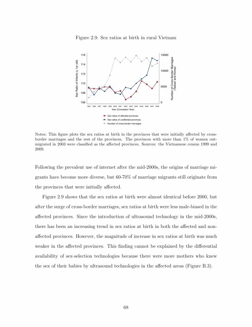
Figure 2.9: Sex ratios at birth in rural Vietnam

0

5000

10000

15000

Num

ber o

f Cro

ss-B

orde

r Mar

riage

s(T

aiw

an a

nd K

orea

)

106

108

110

112

114

116

Sex

Rat

io o

f Inf

ants

(≤ 1

yr o

ld)

1995 1996 1997 1998 1999 2000 2001 2002 2003 2004 2005 2006 2007 2008

Year (Conception Year)

Sex ratios of affected provincesSex ratios of unaffected provincesNumber of cross-border marraiges

Notes: This figure plots the sex ratios at birth in the provinces that were initially affected by cross-border marriages and the rest of the provinces. The provinces with more than 1% of women out-migrated in 2003 were classified as the affected provinces. Sources: the Vietnamese census 1999 and2009.

Following the prevalent use of internet after the mid-2000s, the origins of marriage mi-

grants have become more diverse, but 60-70% of marriage migrants still originate from

the provinces that were initially affected.

Figure 2.9 shows that the sex ratios at birth were almost identical before 2000, but

after the surge of cross-border marriages, sex ratios at birth were less male-biased in the

affected provinces. Since the introduction of ultrasound technology in the mid-2000s,

there has been an increasing trend in sex ratios at birth in both the affected and non-

affected provinces. However, the magnitude of increase in sex ratios at birth was much

weaker in the affected provinces. This finding cannot be explained by the differential

availability of sex-selection technologies because there were more mothers who knew

the sex of their babies by ultrasound technologies in the affected areas (Figure B.3).

68

2.6 Conclusion

This chapter empirically examines the economic impacts of marriage migration in both

migrant-sending and migrant-receiving countries by answering four questions: (i) who

moves, (ii) who benefits, (iii) who loses, and (iv) to what extent. I show that the se-

lection of migrants is governed by the demographic structures and economic conditions

of countries involved and by the costs of cross-border marriage. Agents with low SES

cannot engage in cross-border marriage due to the associated costs. Agents with high

SES in the wealthier country also do not marry across borders because they can secure

better domestic partners. I also find that the long sides of the marriage markets bene-

fit, and the short sides lose from the lowered cost of cross-border marriage on various

margins. Through marriage market equilibrium effects, the flows of marriage migrants

affect not only the direct marital outcomes but also the respective power of all men

and women in both countries by altering their shadow prices in the markets.

The situation in Taiwan and Vietnam may seem unique in several ways. However,

there are many other examples of marriage markets that actively interact. For exam-

ple, there are up to 300,000 Turkish-Russian married couples, and the spousal category

accounted for 40% of migrant settlements in the UK in 2009 (Charsley et al. (2012)).

Other European countries, including Spain, France, and Switzerland, have also expe-

rienced an increase in the number of cross-border marriages in the past two decades,

which could be explained by the negligible associated costs within the European Union.

Moreover, long-lasting sex ratio imbalances in China and India may affect the dynamics

of the neighboring countries’ marriage markets. The theoretical framework presented

in the first chapter and empirical evidence in this chapter shed light on why this phe-

nomenon takes place, who becomes a marriage migrant and to what extent this can

affect the welfare of local people.

This chapter also illustrates the implications of cost-changing policies for marriage

69

markets and women’s power. Many countries faced with increasing immigration, includ-

ing Taiwan, South Korea, Denmark and the Netherlands, have implemented restrictive

immigration policies. The results of this paper suggest that such policies can have broad

influences on populations, as they can affect the economic decisions of every man and

woman in countries involved, not just those who are in or considering cross-border mar-

riages. In countries with male-skewed sex ratios, lowering the cost of entry for women

from other countries can certainly mitigate the imbalances in the marriage market.

However, at the same time, it can decrease local women’s power within households.

These findings highlight that related costs and benefits should be carefully weighed

when designing immigration policies.

70

Chapter 3

Improving Job Matching Among

Youth

So Yoon Ahn, Rebecca Dizon-Ross, and Benjamin Feigenberg

71

3.1 Introduction

There is a growing consensus that youth unemployment in less developed countries is a

major economic and social problem. The problem is particularly severe in the Middle

East and North Africa (MENA) region. More than 28 percent of MENA youth were

estimated to be unemployed in 2014, which is the highest rate across all regions (In-

ternational Labour Organization (2015)). High youth unemployment has far-reaching

implications that extend beyond the economic sphere; the failure to successfully inte-

grate youth into the labor market is seen as a major contributor to the rise of the “Arab

Spring,” for example (Malik and Awadallah (2013)).

The development of online job matching portals that connect employers with po-

tential employees is one strategy to promote youth employment. Although online job

search is a relatively recent phenomenon in MENA countries, its importance has been

rapidly increasing. Internet usage has been rising across most of the developing world;

between 2010 and 2015, in Arab countries, the Internet penetration rate almost dou-

bled, reaching the world average penetration rate of 44% in 2015. The reliance on

online job search in the wider MENA region is correspondingly high and rising, with

for example over 30% of unemployed youth in Egypt and over 40% in the Palestinian

territories using online search. Consequently, as highlighted in a recent World Bank

report, private sector online search portals have the potential to play a critical role in

reducing labor market frictions that hinder youth employment, even among low-income

populations (Raja et al. (2013)).

This research includes several experiments conducted with online jobseekers and

employers. The experiments aim to understand how to improve the efficiency of job

search activities and ultimately increase jobseeker-employer match rates. This research

is being conducted in collaboration with two online websites, Silatech and Bayt.com,

which collectively operate many different web portals with over 12 million registered

72

users, presence in 40 countries, and constitute the largest online job presence in the

MENA region. In addition to having the potential to directly improve the efficiency of

the hiring process, studying online search provides us with a nice opportunity to shed

light on the barriers to employment because of the rich data on behavior we can collect

through the websites.

In collaboration with our implementing partners, we have worked over the previous

two years to identify job portal-related issues that may lead to suboptimal rates of job

matching. This process evaluation identified poor targeting of applications by jobseek-

ers – and associated “congestion” caused by too many applications from poorly qualified

applicants – as the major challenges. Each of the proposed experiments (described in

detail below) tests an alternative possible mechanism that may constrain successful

employer-jobseeker matching. In line with recent discussions that highlight the need

for economists to engage with the details of policy making and program design (Duflo

(2017)), we believe that this approach is well-suited to identifying and implementing

a set of low-cost adjustments to existing technologies that have large potential payoffs

for both employers and jobseekers.

To improve our understanding of the types of interventions that may be most ef-

fective in reducing congestion and promoting better targeting of applications, we have

conducted a pilot study in eight countries in the MENA region.1 The hypothesis mo-

tivating the study is that one reason jobseekers may not target their applications well

is that they lack accurate information about their job market competitiveness. Indeed,

anecdotal evidence suggests that changing regional labor markets, and a reduction in

the public employment share in particular, have led jobseekers to have unrealistically

high expectations for the types of employment their credentials entitle them to obtain.

1They are Algeria, Egypt, Iraq, Lebanon, Morocco, Palestine, Qatar, and Tunisia. Among thesecountries, the data for Iraq are the largest since its experiment started in September 2015 whereas theexperiments in other countries started in April 2017.

73

As a result, our experiment provides randomly-selected jobseekers with information on

their competitiveness relative to other applicants for a given job posting (as rated by

an internal algorithm based on factors like education, experience, etc.).

In order to understand the impacts of information regarding competitiveness on

job search behavior, we first investigate the total number of views and applications of

jobseekers in the control and treatment groups. We do not find any meaningful dif-

ferences in the total number of views and applications for the control and treatment

groups. Next, we examine the total number of applications by rankings. Interestingly,

we find that the treatment group that received the information on jobseeker’s competi-

tiveness shows increase in the number of applications for the jobs where jobseekers were

ranked above median. This result suggest that reducing such information asymmetries

improves the targeting of jobseekers’ applications.

Our subsequent analysis on jobseeker-job level data bolsters the findings at the

jobseeker level. We analyze the ranking distributions of job views and applications for

the jobseekers who are in the control and treatment groups, respectively. If jobseekers

have incomplete information on their own competitiveness, we should observe that the

overall ranking distributions should be higher for the treatment group since they would

adjust their job search behavior towards the jobs where they are better evaluated.

The results fully support this prediction: the jobseekers who received the information

on jobseeker’s competitiveness viewed jobs where they were more highly ranked for.

Moreover, the jobseekers who received the information on competitiveness applied for

the jobs where they were more competitive compared to the jobseekers in the control

group.

Heterogeneity analysis results show that there is a large variation in terms of the sizes

of treatment effects. We find that the impacts of information are the largest for entry-

level jobseekers and those with bachelors degree, who face the highest unemployment

74

rates in the region and whose baseline job targeting is worse than other jobseekers.

Our results suggest that cost-effective treatments on online job platform can potentially

improve aggregate labor market outcomes because entry-level jobseekers and jobseekers

with bachelors degree who lack accurate information use internet the most frequently

in the region.

An extensive theoretical and empirical literature explores inefficiencies in job search

behavior in developed country settings, and recent work has focused on using U.S.-

based online jobs portals data to better understand constraints to employer-jobseeker

match rates (Krueger and Mueller (2010), Gee (2017), Pallais (2014)). In contrast,

we have a much more limited understanding of the importance of job search frictions

in developing country settings, and in the MENA region in particular. Existing work

in the MENA region and other developing countries has instead focused primarily on

evaluating the importance of traditional active labor market interventions, such as the

provision of publicly-subsidized internships (see, for instance, McKenzie et al. (2016)).

Descriptive evidence on job search behavior in the MENA region suggests that the

lessons learned from existing work about how to improve the efficiency of online job

search in developed country settings may not be readily applicable. Indeed, rapid

demographic change (known as the “youth bulge”) and corresponding changes in the

labor market suggest that information frictions may be particularly problematic in this

environment, consistent with the previous study showing that information frictions can

be particularly acute in developing country settings (Dizon-Ross (2017)). Our research

extends the study of job search frictions to the highly policy-relevant MENA region, and

identifies and tests low-cost interventions that can substantially improve the welfare of

both jobseekers and employers.

We contribute to the existing job search literature by highlighting the importance

of a new type of misinformation: jobseekers’ inaccurate beliefs about their own relative

75

competitiveness. The previous literature on this type of misinformation is only theoret-

ical and lab-experimental (Falk et al. (2006b), Falk et al. (2006a), Spinnewijn (2015)).

It has also focused on a different type of misinformation related to “general” (i.e.,

population-average) information about job search, such as the labor market conditions

or the average number of other applicants (e.g., Altmann et al. (2015), Gee (2017)).

We build on the emerging literature on the importance of “individually-tailored” infor-

mation in labor markets (Belot et al. (2015)) by investigating the impacts of providing

a new type of individual-specific information (namely, applicants’ “relative competi-

tiveness”).

The rest of this chapter is organized as follows. Section 3.2 provides background

information on our partnership and poor targeting behavior of jobseekers on the portals.

Section 3.3 explains the experimental design. Section 3.4 present the findings. Section

3.5 concludes.

3.2 Background

3.2.1 Setting

This research is being conducted in collaboration with two affiliated job websites: Silat-

ech, which runs online job-search portals in eight MENA countries (Algeria, Egypt,

Iraq, Lebanon, Morocco, Palestine, Qatar, and Tunisia), and Bayt.com, which oper-

ates online job-search portals in over 30 countries, with the largest penetration in the

MENA region. Silatech is a non-profit organization that has partnered with Microsoft

to make their platform one of the largest employability portals in the region, while

Bayt.com is a for-profit organization that is the largest portal in the region. Both

Silatech and Bayt.com are keenly interested in evidence-based program design. Our

partnership began in 2015 with a particular focus in Silatech’s portal in Iraq and it has

76

grown to include all eight Silatech countries at present. With Silatech’s support, we

have obtained access to a rich array of data that includes data collected from the CVs

submitted by all jobseekers, and information on jobseekers’ search behavior, submitted

job applications, the universe of participating firms and job postings, and employer be-

havior, including which CV’s they view and which jobseekers they then request contact

information for. For all job view-level observations, we have also collected information

on the ranking of each jobseeker, as calculated based on Silatech’s in-house ranking

algorithm. Our partnership with Bayt.com, which was facilitated by Silatech, is more

recent, but Bayt.com has already implemented our first experiment on their platform

and we are working with them to obtain all of the data corresponding to the data we

gathered from Silatech. While the Silatech portals on which our pilot experiment was

first launched are marketed primarily to youth in the region, Bayt’s online job search

portals cover the full universe of jobseekers. Thus, the expansion of research activities

to the Bayt platform will help us to learn more about the generalizability of lessons

learned on the Silatech site, where users are younger, to the full population. This dis-

sertation focuses on the results obtained from our pilot experiment conducted on eight

Silatech portals from September 2015 to March 2018.

3.2.2 Evidence on Poor Ex-ante Targeted Search

In collaboration with the implementing partners, we have worked over the last two

years to identify portal-related issues that may lead to suboptimal rates of job match-

ing. This process evaluation identified poorly targeted applications and corresponding

application congestion as a significant challenge for employers posting jobs on the site.

Specifically, employers appear to receive an excessive number of applications from job-

seekers who do not have the appropriate qualifications for the relevant job posting. This

issue was highlighted in qualitative interviews with employers, and is also apparent in

77

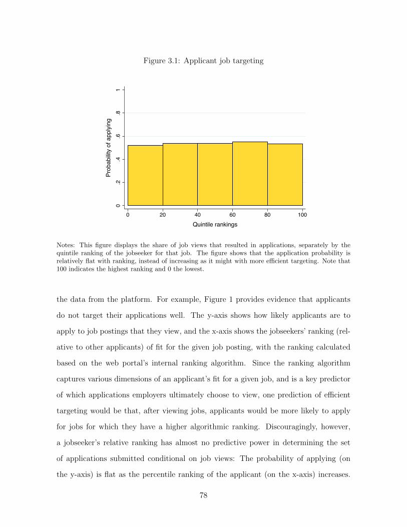
Figure 3.1: Applicant job targeting

0.2

.4.6

.81

Prob

abilit

y of

app

lyin

g

0 20 40 60 80 100

Quintile rankings

Notes: This figure displays the share of job views that resulted in applications, separately by thequintile ranking of the jobseeker for that job. The figure shows that the application probability isrelatively flat with ranking, instead of increasing as it might with more efficient targeting. Note that100 indicates the highest ranking and 0 the lowest.

the data from the platform. For example, Figure 1 provides evidence that applicants

do not target their applications well. The y-axis shows how likely applicants are to

apply to job postings that they view, and the x-axis shows the jobseekers’ ranking (rel-

ative to other applicants) of fit for the given job posting, with the ranking calculated

based on the web portal’s internal ranking algorithm. Since the ranking algorithm

captures various dimensions of an applicant’s fit for a given job, and is a key predictor

of which applications employers ultimately choose to view, one prediction of efficient

targeting would be that, after viewing jobs, applicants would be more likely to apply

for jobs for which they have a higher algorithmic ranking. Discouragingly, however,

a jobseeker’s relative ranking has almost no predictive power in determining the set

of applications submitted conditional on job views: The probability of applying (on

the y-axis) is flat as the percentile ranking of the applicant (on the x-axis) increases.

78

Inaccurate application targeting tends to be particularly problematic in the middle of

the education distribution (defined to include those with bachelor’s degrees or diplo-

mas), for younger jobseekers (defined to include those who are younger than 25), and

for entry-level jobseekers (i.e., those with no previous employment experience). These

findings are consistent with worse targeting among those jobseekers who face greater

employment hurdles in the labor market, as measured by existing studies of unemploy-

ment trends in the MENA region (Devarajan and Mottaghi (2014)). Congestion and

poor targeting may negatively affect employers who find it costly to search through

an excessive number of poorly-matched applications. Moreover, congestion may lead

jobseekers to waste effort on job applications that are unlikely to lead to hires, may

cause dampened motivation when jobseekers’ applications are systematically rejected,

and/or may lead jobseekers to miss out on promising job opportunities that they do

not realize are a good fit for them.2

3.3 Experimental Design

In order to improve targeting behavior of jobseekers, reduce congestion, and ultimately

enhance job-jobseeker match rates, we conducted a pilot study that evaluated the im-

pact of providing tailored information to online jobseekers. Specifically, the study

employed two treatment arms which modified the information presented to jobseekers

on eight website portals. The objective of the treatments was to nudge jobseekers to

target their applications towards jobs with fewer existing applicants and towards job

postings that better matched their skills and experience. Since jobseekers may lack

basic information about their competitiveness for the job market, providing data on

2Note that the evidence is only suggestive; the results are also consistent with jobseekers makingpersonally-efficient application decisions based on factors other than their (perceived) competitivenessfor a given job; an experiment is needed to distinguish whether this lack of targeting indeed reflectsjobseeker “mistakes”.

79

their own qualifications relative to other applicants could potentially have significant

effects on search behavior. Importantly, the informational treatments did not impose

any burden on jobseekers as jobseekers were free to ignore this additional information

or to make use of it in whatever way they saw fit.

More specifically, the research design of the pilot study entailed the randomization

of all the new jobseekers who registered over the course of over two years on eight

Silatech website portals to one of the following three groups:

1. Pure Control (C): Status quo (No information about other applicants.)

2. Treatment group 1 (T1) (Plays role of control in the design): When these users

viewed a job posting on the site, in addition to seeing the standard job posting

seen by the control group, they also received information on how many other

users had applied to the posting.

3. Treatment group 2 (T2) (Treatment of interest): When these users viewed a job

posting on the site, in addition to seeing what treatment group T1 saw, they

also saw information on how they would “rank” relative to the existing appli-

cants. The ranking measure is based on the same algorithm ranking developed

by our partners and used to order applications when viewed by employers. This

algorithm “matters” in this setting, as it has predictive power for which CV’s

employers choose to view and request contact details for.

This randomized design allows us to precisely evaluate the effects of each treatment.

Our primary goal was to evaluate the effect of providing information about a jobseeker’s

relative competitiveness (T2). However, our implementing partner instructed us that

the most transparent way to provide this information in this context was to express

competitiveness as a ranking (“you would be ranked X out of Y applicants who have

80

applied.”). Since this implicitly delivers information on the total number of applicants,

which could independently affect behavior, we provided that information to the T1

group to enable clean comparisons. Specifically, comparing T1 to C shows us the effect

of delivering information on how many users had applied; comparing T2 to T1 (the

comparison of most interest) shows the additional impact of providing information

about an individual jobseeker’s competitiveness.

3.3.1 Summary and Balance Statistics

The summary statistics for the jobseekers in the experiment are presented in Table

3.1. 28% of jobseekers are females, and average age is 28.2 years old, confirming that

the large shares of jobseekers on Silatech portals are young users. Consistent with the

education patterns in the MENA region, the jobseekers on the portal are very well-

educated; only 6% of jobseekers are with high school education or lower than that.

Overall, jobseekers in the control and treatment groups are similar on observable char-

acteristics. There is a marginally statistically significant difference in the experiences

between the C and T1 groups, but the magnitude of this difference is very small.

3.4 Results

In this section, the results at jobseeker level and at jobseeker-job view level are pre-

sented. In the first subsection, the results regarding number of views and applications

at jobseeker level are presented. In the second and third subsection, the results on the

jobseeker-job view level analysis on views and applications are provided. In the fourth

subsection, the results from the heterogeneity analysis by education and career-level

are presented.

81

Table 3.1: Summary statistics: jobseekers

Full sample C T1 T2 T1 – C T2 – C

Mean SD Mean Mean Mean Mean SE Mean SE

(1) (2) (3) (4) (5) (6) (7) (8) (9)

Female 0.275 0.447 0.278 0.270 0.278 -0.008 0.010 0.001 0.010Age 28.2 6.8 28.2 28.3 28.2 0.1 0.2 0.1 0.2Education level:

High school 0.060 0.237 0.059 0.060 0.060 0.001 0.005 0.001 0.005Diploma 0.169 0.375 0.169 0.173 0.165 0.004 0.009 -0.004 0.009Bachelor 0.544 0.498 0.555 0.542 0.537 -0.013 0.011 -0.018 0.011Master or PhD 0.094 0.291 0.089 0.091 0.101 0.002 0.007 0.011 0.007Education info missing 0.133 0.340 0.128 0.135 0.137 0.006 0.008 0.009 0.008

Career level:Entry level 0.197 0.398 0.202 0.196 0.193 -0.005 0.009 -0.009 0.009Mid career 0.402 0.490 0.406 0.401 0.397 -0.005 0.011 -0.009 0.011Management 0.166 0.372 0.158 0.169 0.170 0.011 0.009 0.012 0.009Executive 0.039 0.194 0.040 0.041 0.037 0.001 0.005 -0.003 0.004Senior executive 0.005 0.073 0.006 0.006 0.004 0.000 0.002 -0.002 0.002Career level info missing 0.191 0.393 0.188 0.187 0.199 -0.001 0.009 0.011 0.009

Work experience (inyears)

3.0 4.4 3.0 2.9 3.0 -0.2* 0.1 0.0 0.1

Work experience missing 0.386 0.487 0.385 0.394 0.378 0.009 0.011 -0.008 0.011Last month salary 1640 1430 1665 1648 1608 -17 52 -57 51Last month salary missing 0.587 0.492 0.593 0.586 0.583 -0.007 0.011 -0.011 0.011Number of days after exp.beganc

-132 240 -137 -129 -129 8 6 9 6

Number of observations 11,318 – 3,715 3,813 3,790 – – – –

82

3.4.1 Number of Views and Applications

Our first outcomes of interest are the numbers of views and applications at jobseeker

level. There is no clear prediction that information on competitiveness would affect

the total number of views and applications submitted. To understand the impacts of

information on competitiveness, the following model is estimated:

Yi = α + β1T1i + β2T2i + εi

where Ti is a binary variable which takes 1 if the jobseeker is in T1 and 0 otherwise.

T2i is 1 if the jobseeker is in T2 and 0 otherwise. Robert standard errors are used.

Table 3.2 provides the results on the number of total views and applications sub-

mitted. The overall patterns show that information on the number of other applicants

and information on relative rankings do not significantly affect the number of job views

or applications submitted. Only for the log number of applications, conditional on ap-

plying, there exists marginally meaningful difference between the jobseekers in T1 and

the jobseekers in the control group, suggesting that the information on the number of

other applicants somewhat discourages the number of applications. The results suggest

that overall, our information treatments do not change the level of activities including

views and applications on the job platforms.

However, if we redefine the outcomes as the number of applications by the rankings,

we find that the number of applications with rankings below median decreased for the

jobseekers in T2. Figure 3.2 shows the results. This result suggests that although

the total number of applications submitted did not change for the treatment group

compared to the control group, the composition of applications changed, lowering the

number of applications below the median.

83

Table 3.2: Effect on volume of views or applications

Controlmean

T1 T2 Obs.

(1) (2) (3) (4)

Number of jobs viewed, unconditional 14.622 -0.370 -0.217 11,318(0.571) (0.603)

IHS number of jobs viewed 2.561 -0.024 -0.036 11,318(0.028) (0.028)

Log number of jobs viewed, conditional on viewing 1.822 -0.025 -0.037 11,318(0.030) (0.030)

Applied to any job (=1) 0.807 0.009 0.015 11,318(0.009) (0.009)

Number of jobs applied to, unconditional 7.897 -0.192 -0.097 11,318(0.385) (0.396)

IHS number of jobs applied 1.812 -0.017 -0.002 11,318(0.030) (0.030)

Log number of jobs applied to, conditional on applying 1.497 -0.050* -0.042 9,219(0.030) (0.030)

Notes: This table displays the results from regressing each dependent variable listed in the first column on a dummy for being inany treatment (T) and a dummy for being in T2. IHS refers to inverse hyperbolic sine transformation. Robust standard errors inparentheses. Significance levels: * 10%, ** 5%, *** 1%.

84

Figure 3.2: Treatment effects: Number of applications submitted

A. Number of applications B. IHS(number of applications)

-0.22

0.01

p-value = 0.23

-.6-.4

-.20

.2T2

- C

Below median Above medianControl mean: below median = 3.24; above median = 3.87

Whole sample

-0.03

-0.01

p-value = 0.54

-.08

-.06

-.04

-.02

0.0

2T2

- C

Below median Above medianControl mean: below median = 0.97; above median = 1.25

Whole sample

Notes: The figures display the coefficient on T2 from a seemingly unrelated estimation after regressinga dummy variable for having a below-/above-median ranking when applying on a dummy for being inT1 and a dummy for being in T2. In the left figure (panel A), the dependent variable is the number ofapplications submitted by below-/above-median-ranked jobseekers, whereas in the right figures (panelB), it is the inverse hyperbolic sine transformation of the number of applications submitted. Thevertical red lines for the below-median bars represent 95% confidence intervals, computed using robuststandard errors.

3.4.2 Distributions of Views and Applications

In this section, we analyze jobseeker-job level data as opposed to jobseeker level data

in the previous section. Specifically, we examine the distributions of number of other

applicants for views and applications for T1. For T2, we investigate the distributions

of rankings of views and applications. We estimate the following model:

Yij = α + β1T1i + β2T2i + εij

where i and j indicates jobseekers and jobs, respectively. T1i and T2i are defined in

the same way as in the previous section.

Figure 3.3 shows descriptive patterns of views and applications for C and T1. The

top panels show the distributions of views and applications by the number of other

applicants. These figures suggest that when information on the number of other ap-

85

plications is given, jobseekers view and apply to jobs which have smaller number of

applications. The below panels show the distributions of views and applications for C

and T2. Although the impact sizes are not huge, the figures show that the distributions

of T2 are less concentrated in the lower rankings.

Figure 3.4 presents regression results, confirming the descriptive patterns. When

the number of other applications is small (< 50), jobseekers in T1 are more likely to

view and apply to the job. However, if the number of applications are larger than 50,

jobseekers in T1 have smaller number of views and applications compared to the job-

seekers in the control group. The below panels show the results for T2, showing that the

applications move towards to higher ranked jobs if the jobseekers are given information

on relative rankings. However, the coefficients are not statistically significant.

3.4.3 Application Decisions After Viewing

In this subsection, we analyze application decisions of jobseekers after viewing the jobs

using jobseeker-job level data. If jobseekers do not have accurate estimates of rankings,

and if rankings affect the decisions of them, we would expect to see different effects on

application behavior when the rankings are different. We use the same specification

in the previous section for jobseeker-job level data with application dummy as the

dependent variable. However, to explore whether different rankings inform jobseekers

and change their behavior differently, we also interact the rankings with the treatment

(T2).

The results are given in Figure 3.5 and Table 3.3. The results suggest that the

jobseekers with rankings above 60th percentile did not show different application be-

havior compared to the control group which did not receive any information. However,

the jobseekers who viewed rankings below 60th percentile decreased their applications

modestly. The regression results when continuous percentile rankings are interacted

86

Figure 3.3: Descriptive patterns of job views and applications

0.5

11.

52

Num

ber o

f vie

ws

per j

obse

eker

0 50 100 150 200 250 >300

Number of other applicants

C T1

Job views

0.2

.4.6

.8N

umbe

r of a

pplic

atio

ns p

er jo

bsee

ker

0 50 100 150 200 250 >300


C T1

Job applications

0.5

11.

5N

umbe

r of v

iew

s pe

r job

seek

er

0 20 40 60 80 100

Percentile rankings

C T2

Job views

0.5

11.

5N

umbe

r of a

pplic

atio

ns p

er jo

bsee

ker

0 20 40 60 80 100

Percentile rankings

C T2

Job applications

Notes: The top figures display the average number of views (left) and applications (right) per jobseekerfor each 5 other applicants range for C and T1. The bottom figures show the average number of views(left) and applications (right) per jobseekers for each 5-percentile-ranking range for C and T2.

87

Figure 3.4: Treatment effects-.0

10

.01

.02

.03

T1 -

C

0-50 50-100 100-150 150-200 200-250 250-300


Job views

-.02

0.0

2.0

4T1

- C

0-50 50-100 100-150 150-200 200-250 250-300


Job applications

-.1-.0

50

.05

.1T2

- C

0-20 20-40 40-60 60-80 80-100

Quintile ranking

Job views

-.1-.0

50

.05

.1T2

- C

0-20 20-40 40-60 60-80 80-100

Quintile ranking

Job applications

Notes: The top figures show the coefficient on T1 from a regression of a dummy for being in agiven number of other applicants on a dummy for being in T1 and a dummy for being in T2, withstandard errors are clustered at the jobseeker level. The below figures show the coefficient on T2 froma regression of a dummy for being in a given number of other applicants on a dummy for being in T1and a dummy for being in T2, with standard errors are clustered at the jobseeker level. The sampleis restricted to job views in the left figures and to job applications in the right figures. The shadedareas correspond to 95% confidence intervals.

88

with T2 shown in Table 3.3 show similar patterns. Low rankings discourage the appli-

cations and the discouragement effects significantly decreases as the ranking increases.

To understand whether there exist some groups which are more reactive to information,

we explore heterogenous effects in the next section.

3.4.4 Heterogeneous Effects

The degree of incomplete information may be different across different types of jobseek-

ers. Perhaps, jobseekers with more experiences understand labor market conditions and

where they stand better than jobseekers with relatively short experiences. Also, given

that the supply of educated jobseekers has changed fast in the MENA region, educated

jobseekers may have less accurate information on their competitiveness. To test these

hypotheses, we investigate heterogenous treatment effects by education and career-level.

Figures 3.6 – 3.9 present the distributions of views and applications by education

and career levels. These figures show that treatment effects of T2 vary substantially

across different groups. For both views and applications, the distributional differences

are the largest for jobseekers with bachelors degree and for the entry-level jobseekers. In

particular, the applications of entry-level jobseekers are much less concentrated in the

lower rankings for the jobseekers in T2 group compared to the jobseekers in the control

group. For masters and PhD, T2 decrease the number of views and applications for

almost all ranking ranges except at the very top, but the decrease is more pronounced

for lower-ranked ranges.

Table 3.4 and Table 3.5 present heterogenous effects on application decision after

view by education and by career level. Consistent with other results, jobseekers with

bachelor degree and entry level job seekers are the most responsive to the ranking

information. In particular, jobseekers who viewed jobs with below median rankings

applied to the job 6 percentage point less than those above median.

89

Figure 3.5: Applicant decision after viewing

0.1

.2.3

.4.5

.6Pr

obab

ility

of a

pply

ing

0 20 40 60 80 100

Quintile rankings

C T2

-.1-.0

50

.05

.1

T2 -

C

0-20 20-40 40-60 60-80 80-100

Quintile rankings

Notes: The top figure shows the probability of applying (or the share of jobseekers who applied) foreach quintile, by treatment group. The bottom figure displays the coefficient on T2 × 1{quintile} froma regression of a dummy for having applied on a dummy for being in any treatment, a dummy forbeing in T2, a dummy for being in a given quintile and its interactions with each treatment dummyvariable. The shaded areas correspond to 95% confidence intervals (computed from jobseeker-levelclustered standard errors).

90

Table 3.3: Effect on application decision after view

Dependent variable: Applied to a job (=1)

(1) (2) (3) (4) (5) (6)

T1 -0.000 -0.001 -0.004 -0.003 0.004 0.002(0.012) (0.012) (0.020) (0.019) (0.013) (0.012)

T1 × Number other applicants (÷100) -0.004 -0.004 -0.005 -0.004(0.004) (0.004) (0.004) (0.004)

T2 -0.010 -0.006 -0.034 -0.030 -0.001 0.003(0.013) (0.013) (0.022) (0.021) (0.014) (0.013)

T2 × Percentile ranking 0.045∗ 0.043∗

(0.026) (0.025)

T2 × Below median -0.017 -0.017(0.014) (0.013)

Include controls? No Yes No Yes No Yes

Control mean 0.505 0.505 0.505 0.505 0.505 0.505

Observations 156,965 156,965 156,965 156,965 156,965 156,965

Notes: Control variables include gender, years of experience, last month salary, number of days since registration, and dummiesfor age categories, education levels, career levels. Regressions also include the main effects of number of applicants (÷100) and ofpercentile ranking in Columns (3) and (4), and they include the main effects of being ranked below median in Columns (5) and (6).Standard errors are clustered at the jobseeker level in parentheses. Significance levels: * 10%, ** 5%, *** 1%.

91

Figure 3.6: Descriptive patterns of job views, by education level

0.5

11.

52

Num

ber o

f vie

ws

per j

obse

eker

0 20 40 60 80 100

Percentile rankings

C T2

High school

0.5

11.

52

Num

ber o

f vie

ws

per j

obse

eker

0 20 40 60 80 100

Percentile rankings

C T2

Diploma

0.5

11.

52

Num

ber o

f vie

ws

per j

obse

eker

0 20 40 60 80 100

Percentile rankings

C T2

Bachelors

0.5

11.

52

Num

ber o

f vie

ws

per j

obse

eker

0 20 40 60 80 100

Percentile rankings

C T2

Masters or PhD

Notes: The figures display the average number of job views per jobseeker for each 5-percentile-rankingrange, by treatment group. Each figure corresponds to a different education-level sample.

92

Figure 3.7: Descriptive patterns of job views, by career level

0.5

11.

52

Num

ber o

f vie

ws

per j

obse

eker

0 20 40 60 80 100

Percentile rankings

C T2

Entry level

0.5

11.

52

Num

ber o

f vie

ws

per j

obse

eker

0 20 40 60 80 100

Percentile rankings

C T2

Management

0.5

11.

52

Num

ber o

f vie

ws

per j

obse

eker

0 20 40 60 80 100

Percentile rankings

C T2

Mid career

0.5

11.

52

Num

ber o

f vie

ws

per j

obse

eker

0 20 40 60 80 100

Percentile rankings

C T2

Executive or senior executive

Notes: The figures display the average number of job views per jobseeker for each 5-percentile-rankingrange, by treatment group. Each figure corresponds to a different career-level sample.

93

Figure 3.8: Descriptive patterns of job applications, by education level

0.2

.4.6

.81

Num

ber o

f app

licat

ions

per

jobs

eeke

r

0 20 40 60 80 100

Percentile rankings

C T2

High school

0.2

.4.6

.81

Num

ber o

f app

licat

ions

per

jobs

eeke

r

0 20 40 60 80 100

Percentile rankings

C T2

Diploma

0.2

.4.6

.81

Num

ber o

f app

licat

ions

per

jobs

eeke

r

0 20 40 60 80 100

Percentile rankings

C T2

Bachelors

0.2

.4.6

.81

Num

ber o

f app

licat

ions

per

jobs

eeke

r

0 20 40 60 80 100

Percentile rankings

C T2

Masters or PhD

Notes: The figures display the average number of job applications per jobseeker for each 5-percentile-ranking range, by treatment group. Each figure corresponds to a different education-level sample.

94

Figure 3.9: Descriptive patterns of job applications, by career level

0.2

.4.6

.81

Num

ber o

f app

licat

ions

per

jobs

eeke

r

0 20 40 60 80 100

Percentile rankings

C T2

Entry level

0.2

.4.6

.81

Num

ber o

f app

licat

ions

per

jobs

eeke

r

0 20 40 60 80 100

Percentile rankings

C T2

Management

0.2

.4.6

.81

Num

ber o

f app

licat

ions

per

jobs

eeke

r

0 20 40 60 80 100

Percentile rankings

C T2

Mid career

0.2

.4.6

.81

Num

ber o

f app

licat

ions

per

jobs

eeke

r

0 20 40 60 80 100

Percentile rankings

C T2

Executive or senior executive

Notes: The figures display the average number of job applications per jobseeker for each 5-percentile-ranking range, by treatment group. Each figure corresponds to a different career-level sample.

95

Table 3.4: Heterogeneous effects on application decision after view, by education level

Panel A. High school


(1) (2) (3) (4) (5) (6)

T1 0.016 -0.000 -0.011 -0.019 0.039 0.020(0.045) (0.043) (0.075) (0.075) (0.049) (0.045)

T1 × # apps (/100) -0.018 -0.019 -0.019 -0.020(0.016) (0.016) (0.016) (0.016)

T2 0.049 0.038 -0.045 -0.051 0.052 0.039(0.051) (0.048) (0.091) (0.088) (0.051) (0.045)

T2 × Percentile ranking 0.125 0.117(0.105) (0.097)

T2 × Below median -0.054 -0.048(0.055) (0.052)


Control mean 0.445 0.445 0.445 0.445 0.445 0.445

Observations 8,867 8,867 8,867 8,867 8,867 8,867

Panel B. Diploma


(1) (2) (3) (4) (5) (6)

T1 -0.020 -0.019 -0.011 -0.007 -0.029 -0.030(0.030) (0.028) (0.046) (0.044) (0.032) (0.031)

T1 × # apps (/100) 0.000 0.001 0.000 0.001(0.005) (0.005) (0.005) (0.005)

T2 -0.013 -0.024 -0.039 -0.066 -0.007 -0.012(0.031) (0.028) (0.046) (0.043) (0.035) (0.033)


T2 × Below median -0.013 -0.026(0.030) (0.029)


Control mean 0.515 0.515 0.515 0.515 0.515 0.515

Observations 27,966 27,966 27,966 27,966 27,966 27,966

96

Panel C. Bachelors


(1) (2) (3) (4) (5) (6)

T1 -0.006 -0.005 -0.009 -0.005 -0.008 -0.008(0.015) (0.015) (0.026) (0.025) (0.016) (0.016)

T1 × # apps (/100) 0.002 0.001 0.002 0.001(0.004) (0.004) (0.004) (0.004)

T2 -0.021 -0.014 -0.046∗ -0.041 -0.012 -0.005(0.017) (0.016) (0.028) (0.027) (0.018) (0.018)


T2 × Below median -0.022 -0.023(0.017) (0.017)


Control mean 0.526 0.526 0.526 0.526 0.526 0.526

Observations 95,348 95,348 95,348 95,348 95,348 95,348

Panel D. Masters or PhD


(1) (2) (3) (4) (5) (6)

T1 0.049 0.040 0.024 0.024 0.080∗∗ 0.064∗∗

(0.042) (0.033) (0.061) (0.055) (0.038) (0.030)

T1 × # apps (/100) -0.011 -0.008 -0.011 -0.009(0.007) (0.006) (0.008) (0.006)

T2 -0.009 -0.011 -0.014 -0.016 -0.001 -0.004(0.041) (0.037) (0.066) (0.061) (0.034) (0.031)


T2 × Below median 0.024 0.023(0.038) (0.035)


Control mean 0.449 0.449 0.449 0.449 0.449 0.449

Observations 14,583 14,583 14,583 14,583 14,583 14,583

97

Table 3.5: Heterogeneous effects on application decision after view, by career level

Panel A. Entry Level


(1) (2) (3) (4) (5) (6)

T1 -0.035 -0.035 -0.053 -0.045 -0.030 -0.035(0.025) (0.024) (0.043) (0.040) (0.027) (0.026)

T1 × # apps (/100) -0.002 0.000 -0.002 -0.000(0.005) (0.004) (0.004) (0.004)

T2 0.019 0.019 -0.051 -0.055 0.042 0.041(0.028) (0.027) (0.050) (0.049) (0.031) (0.030)

T2 × Percentile ranking 0.119∗ 0.122∗∗

(0.061) (0.058)

T2 × Below median -0.056∗ -0.058∗

(0.034) (0.032)


Control mean 0.465 0.465 0.465 0.465 0.465 0.465

Observations 31,203 31,203 31,203 31,203 31,203 31,203

Panel B. Management


(1) (2) (3) (4) (5) (6)

T1 -0.050∗ -0.041 -0.072 -0.058 -0.048 -0.039(0.029) (0.027) (0.048) (0.045) (0.030) (0.028)

T1 × # apps (/100) 0.007 0.007 0.007 0.007(0.007) (0.007) (0.007) (0.007)

T2 0.002 0.011 -0.033 -0.031 0.016 0.029(0.029) (0.027) (0.047) (0.044) (0.031) (0.029)


T2 × Below median -0.026 -0.033(0.028) (0.026)


Control mean 0.558 0.558 0.558 0.558 0.558 0.558

Observations 29,546 29,546 29,546 29,546 29,546 29,546

98

Panel C. Mid career


(1) (2) (3) (4) (5) (6)

T1 0.019 0.017 0.025 0.027 0.023 0.020(0.018) (0.018) (0.031) (0.029) (0.019) (0.018)

T1 × # apps (/100) -0.004 -0.005 -0.004 -0.005(0.007) (0.007) (0.007) (0.007)

T2 -0.036∗ -0.037∗ -0.030 -0.028 -0.040∗ -0.041∗∗

(0.021) (0.020) (0.034) (0.033) (0.021) (0.020)

T2 × Percentile ranking -0.009 -0.014(0.039) (0.037)

T2 × Below median 0.010 0.012(0.020) (0.019)


Control mean 0.519 0.519 0.519 0.519 0.519 0.519

Observations 68,575 68,575 68,575 68,575 68,575 68,575

Panel D. Executive or senior executive


(1) (2) (3) (4) (5) (6)

T1 0.091 0.080∗ 0.001 0.043 0.118 0.085∗

(0.061) (0.044) (0.093) (0.077) (0.075) (0.047)

T1 × # apps (/100) 0.008 0.006 0.007 0.006(0.013) (0.013) (0.013) (0.013)

T2 0.023 0.036 -0.014 0.049 0.042 0.036(0.063) (0.051) (0.095) (0.085) (0.071) (0.050)

T2 × Percentile ranking 0.078 -0.012(0.118) (0.096)

T2 × Below median -0.027 0.014(0.065) (0.051)


Control mean 0.491 0.491 0.491 0.491 0.491 0.491

Observations 6,636 6,636 6,636 6,636 6,636 6,636

99

3.5 Conclusion

We show that providing individually tailored information regarding each jobseeker’s

competitiveness on job search platform can nudge jobseekers to apply for jobs where

they are more competitive. Although further investigation is needed to understand

whether this information treatment actually improves the final match jobseeker-job

outcomes, our results suggest that this cost-effective intervention significantly affects

job-seeking behavior on the platform with better targeted views and applications.

This research is still on-going project and the current analysis can be extended

in three key directions. First, we are in the process of collecting data from belief

surveys. Specifically, we survey jobseekers online at various points in time regarding

their expectations about job search duration and outcomes and regarding their beliefs

about their own labor market competitiveness. By examining the relationship between

the degree of inaccuracy in beliefs and the degree to which jobseekers respond to the

information provided, we will shed light on the extent to which inaccurate beliefs do in

fact drive inefficient job search behavior.

Second, we plan to conduct a survey on final employment outcomes. Since final

job search outcomes, including interview offers, hiring decisions and wage offers, are

currently not observed, we plan to obtain this critical information via survey. This data

on ultimate outcomes will supplement the information on intermediate outcomes that

is currently collected by our partners, including the set of jobseeker CVs viewed by

employers and the set of jobseekers whose contact details are requested by employers.

The activities described above will allow us to comprehensively assess the effects

of misinformation on labor supply, examining whether information frictions negatively

affect jobseeker search behavior and outcomes. However, inaccurate beliefs and poorly

targeted search could also affect employers, leading to congestion that can slow the

match process and potentially lead to more rule-of-thumb or inefficient hiring decisions.

100

To explore this second set of impacts, we are also in the process of expanding this

experiment to new website portals, but changing the way the experiment is structured:

Instead of randomizing the information at the jobseeker-level, as we have done before,

which allows us to uncover the impacts on jobseeker behavior, we will randomize the

information at the job posting level. The job-level randomization will allow us to

analyze the effects of receiving different types of applications on employer behavior,

and speak to the congestion externalities of poorly targeted search. We are currently

developing the infrastructure to access the data from this second experiment.

101

Bibliography

Abramitzky, R., A. Delavande, and L. Vasconcelos (2011): “Marrying up:the role of sex ratio in assortative matching,” American Economic Journal: AppliedEconomics, 124–157.

Altmann, S., F. Armin, S. Jager, and F. Zimmermann (2015): “Learning aboutjob search: A field experiment with job seekers in Germany,” IZA Discussion PaperNo. 9040.

Angrist, J. (2002): “How do sex ratios affect marriage and labor markets? Evidencefrom America’s second generation,” Quarterly Journal of Economics, 997–1038.

Attanasio, O. P. and V. Lechene (2014): “Efficient responses to targeted cashtransfers,” Journal of Political Economy, 122, 178–222.

Banister, J. (1985): The Population of Vietnam, 77, US Department of Commerce,Bureau of the Census.

Belanger, D. and T. G. Linh (2011): “The impact of transnational migration ongender and marriage in sending communities of Vietnam,” Current Sociology, 59,59–77.

Belot, M., P. Kircher, and P. Muller (2015): “Providing advice to job seekersat low cost: An experimental study on on-line advice,” .

Bertoli, S., J. F.-H. Moraga, and F. Ortega (2013): “Crossing the border:Self-selection, earnings and individual migration decisions,” Journal of DevelopmentEconomics, 101, 75–91.

Borjas, G. J. (1987): “Self-selection and the earnings of immigrants.” AmericanEconomic Review, 77, 531–53.

——— (2014): Immigration economics, Harvard University Press.

Browning, M., F. Bourguignon, P.-A. Chiappori, and V. Lechene (1994):“Income and outcomes: A structural model of intrahousehold allocation,” Journal ofPolitical Economy, 1067–1096.

Browning, M., P.-A. Chiappori, and Y. Weiss (2014): Economics of the Family,Cambridge University Press.

Charles, K. K. and M. C. Luoh (2010): “Male incarceration, the marriage market,and female outcomes,” The Review of Economics and Statistics, 92, 614–627.

102

Charsley, K., B. Storer-Church, M. Benson, and N. Hear (2012):“Marriage-Related Migration to the UK,” International Migration Review, 46, 861–890.

Chiappori, P.-A. (2017): Matching with Transfers: The Economics of Love andMarriage, Princeton University Press.

Chiappori, P.-A., B. Fortin, and G. Lacroix (2002): “Marriage market, divorcelegislation, and household labor supply,” Journal of Political Economy, 110, 37–72.

Chiappori, P.-A., R. J. McCann, and L. P. Nesheim (2010): “Hedonic priceequilibria, stable matching, and optimal transport: equivalence, topology, anduniqueness,” Economic Theory, 42, 317–354.

Chiappori, P.-A., R. J. McCann, and B. Pass (2016a): “Multi-to One-Dimensional Optimal Transport,” Communications on Pure and Applied Mathemat-ics.

Chiappori, P.-A., S. Oreffice, and C. Quintana-Domeque (2016b): “Black–White Marital Matching: Race, Anthropometrics, and Socioeconomics,” Journal ofDemographic Economics, 82, 399–421.

——— (2017): “Bidimensional matching with heterogeneous preferences: educationand smoking in the marriage market,” Journal of the European Economic Associa-tion.

Chiquiar, D. and G. H. Hanson (2005): “International migration, self-selection,and the distribution of wages: Evidence from Mexico and the United States,” Journalof Political Economy, 113, 239–281.

Desai, J. (1995): “Vietnam through the Lens of Gender,” Hanoi: UNDP.

Devarajan, S. and L. Mottaghi (2014): MENA Quarterly Economic Brief, July2014: Predictions, Perceptions and Economic Reality-Challenges of the Seven MiddleEast and North Africa Countries Described in 14 Charts, World Bank Publications.

Dizon-Ross, R. (2017): “Parents’ beliefs and children’s education: Experimentalevidence from Malawi,” Working paper.

Do, T. N. T., H. Glind, P. Kelly, G. Kamphuis, M. Heeswijk,D. McArthur, N. Phan, T. Tong, A. Tran, and T. Tran (2003): “Mar-riages of Convenience: Context, processes and results of cross-border marriages be-tween Vietnamese young women and Taiwanese men,” Mobility Research and SupportCenter, Hanoi.

Duflo, E. (2012): “Women Empowerment and Economic Development,” Journal ofEconomic Literature, 50, 1051.

103

——— (2017): “The Economist as Plumber,” NBER working paper.

Edlund, L., E. M. Liu, and J.-T. Liu (2013): “Beggar-Thy-Women: Foreign Bridesand the Domestic Front–The Case of Taiwan,” Working Paper.

Engel, E. (1895): Die Lebenskosten belgischer Arbeiter-Familien fruher und jetzt, C.Heinrich.

Falk, A., D. Huffman, and U. Sunde (2006a): “Do I have what it takes? Equi-librium search with type uncertainty and non-participation,” IZA Discussion PaperNo. 2531.

——— (2006b): “Self-confidence and search,” IZA Discussion Paper No. 2525.

Feigenberg, B. (2017): “Fenced Out: Why Rising Migration Costs Matter,” WorkingPaper.

Fulford, S. L. (2015): “Marriage migration in India: Vast, varied, and misunder-stood,” Tech. rep., Boston College Working Paper 820.

Gee, L. K. (2017): “The More You Know: Information Effects in Job ApplicationRates in a Large Field Experiment,” Working paper.

Goodkind, D. (1997): “The Vietnamese double marriage squeeze,” InternationalMigration Review, 108–127.

International Labour Organization (2015): “Global Employment Trends forYouth 2015,” Policy report.

International Organization for Migration (2015): “Asia-Pacific migrationreport 2015: Migrants’ contribution to development,” .

Kawaguchi, D. and S. Lee (2017): “Brides For Sale: Cross-border Marriages andFemale Immigration,” Economic Inquiry, 55, 633–654.

Krueger, A. B. and A. Mueller (2010): “Job search and unemployment insurance:New evidence from time use data,” Journal of Public Economics, 94, 298–307.

Lam, D., J. Boymal, and B. Martin (2004): “Internet diffusion in Vietnam,”Technology in Society, 26, 39–50.

Lewbel, A. (2008): “Engel curves,” The New Palgrave Dictionary of Economics, 2.

Lichter, D. T., Z. Qian, and D. Tumin (2015): “Whom do immigrants marry?Emerging patterns of intermarriage and integration in the United States,” The AN-NALS of the American Academy of Political and Social Science, 662, 57–78.

Lu, M. C.-W. (2005): “Commercially arranged marriage migration: Case studies ofcross-border marriages in Taiwan,” Indian Journal of Gender Studies, 12, 275–303.

104

——— (2008): “Gender, marriage and migration: contemporary marriages betweenmainland China and Taiwan,” Ph.D. thesis, Research School of Asian, African andAmerindian Studies (CNWS), Faculty of Arts, Leiden University.

Malik, A. and B. Awadallah (2013): “The economics of the Arab Spring,” WorldDevelopment, 45, 296–313.

McKenzie, D., N. Assaf, and A. P. Cusolito (2016): “The demand for, andimpact of, youth internships: evidence from a randomized experiment in Yemen,”IZA Journal of Labor & Development, 5, 1.

Mincer, J. (1978): “Family migration decisions,” Journal of political Economy, 86,749–773.

Minh, T. Q. (2011): “Two decades of Taiwan’s FDI in Vietnam - An Analysis andAssessment,” .

Mizoguchi, N. (2010): “The Consequences of the Vietnam War on the VietnamesePopulation,” .

Moraga, J. F.-H. (2011): “New evidence on emigrant selection,” The Review ofEconomics and Statistics, 93, 72–96.

Morrow, M. and S. Barraclough (2003): “Tobacco control and gender in south-east Asia. Part II: Singapore and Vietnam,” Health Promotion International, 18,373–380.

Nguyen, X. and X. Tran (2010): “Vietnamese-Taiwanese Marriages,” Asian cross-border marriage migration: Demographic patterns and social issues, 157–176.

Oreffice, S. (2011): “Sexual orientation and household decision making.: Same-sexcouples’ balance of power and labor supply choices.” Labour Economics, 18, 145–158.

Pallais, A. (2014): “Inefficient hiring in entry-level labor markets,” The AmericanEconomic Review, 104, 3565–3599.

Raja, S., S. Imaizumi, T. Kelly, J. Narimatsu, and C. Paradi-Guilford(2013): “Connecting to work: how information and communication technologiescould help expand employment opportunities,” Tech. rep., The World Bank.

Rosenzweig, M. R. and O. Stark (1989): “Consumption smoothing, migration,and marriage: Evidence from rural India,” Journal of political Economy, 97, 905–926.

Rubinstein, Y. and D. Brenner (2013): “Pride and prejudice: using ethnic-sounding names and inter-ethnic marriages to identify labour market discrimination,”Review of Economic Studies, 81, 389–425.

Sandell, S. H. (1977): “Women and the economics of family migration,” The Reviewof Economics and Statistics, 406–414.

105

Smith, J. P. and D. Thomas (1998): “On the road: Marriage and mobility inMalaysia,” Journal of Human Resources, 805–832.

Spinnewijn, J. (2015): “Unemployed but optimistic: Optimal insurance design withbiased beliefs,” Journal of the European Economic Association, 13, 130–167.

Tseng, H. (2016): Racialization of Foreign Women in the Transnational MarriageMarket of Taiwan, Cultural Politics of Gender and Sexuality in Contemporary Asia,Chapter twelve.

Wang, H.-z. and S.-m. Chang (2002): “The Commodification of International Mar-riages: Cross-border Marriage Business in Taiwan and Viet Nam,” Internationalmigration, 40, 93–116.

Weiss, Y., J. Yi, and J. Zhang (2017): “Cross-border Marriage Costs and MarriageBehavior: Theory and Evidence,” International Economic Review, Forthcoming.

Yang, W. S. and Y.-y. T. Liu (2014): “Gender imbalances and the twisted marriagemarket in Taiwan,” in The Family and Social Change in Chinese Societies, Springer,117–130.

106

Appendix A

Appendix to Chapter 1

107

A.1 Proof of Proposition 1

Proof. 1. When Y = Y ′

Suppose x ≥ x′ but y′ > y on a subset of positive measure. Consider the surplus

of (x,X), (y, Y ) and (x′, X), (y′, Y ) matches:

Σ1 = ΣXY (x, y) + ΣXY (x′, y′)− 2λ1(X 6= Y )

Switching the matching generates:

Σ2 = ΣXY (x, y′) + ΣXY (x′, y)− 2λ1(X 6= Y )

By supermodularity Σ2 > Σ1. Since x ≥ x′ but y < y′ on a subset of positive

measure, the surplus can be improved by switching. Contradiction.

2. When Y 6= Y ′

Without loss of generality, let Y = X. Suppose x ≥ x′ but y′ > y on a subset

of positive measure. Consider the surplus of (x,X), (y, Y ) and (x′, X), (y′, Y ′)

matches:

Σ1 = ΣXY (x, y) + ΣX′Y (x′, y′) = S(x, y) + S(x′, y′)− λ

Switching the matching generates:

Σ2 = ΣXY (x, y′) + ΣX′Y (x′, y) = S(x, y′) + S(x′, y)− λ

By supermodularity Σ2 > Σ1. Since x ≥ x′ but y < y′ on a subset of positive

measure, the surplus can be improved by switching. Contradiction.

The proof of the second part is similar.


Proof. Without a loss of generality, let X be T . Suppose a man x from country T is

matched to either a woman y from country T or a woman y′ from country V at the

108

stable match. Let uT (x) be his utility. Then, by stability,

uT (x) = maxs

(S(x, s)− vT (s))

= maxs′

(S(x, s′)− λ− vV (s′))

where vT (s) (vV (s′)) is the utility of a woman from country T (a woman from country

V ) with the type s (s′); note that the maximum is reached at s = y and s′ = y′

respectively. By the envelope theorem:

u′T (x) =∂

∂xS(x, y) =

∂

∂xS(x, y′)

Since ∂S∂x

is strictly increasing in y, y = y′.

From the stability conditions, we have

uT (x) = S(x, y)− vT (y)

= S(x, y)− λ− vV (y)

Thus, vV (y) + λ = vT (y).

The second part can be proved similarly.

A.3 Matching Functions of Proposition 4

1. If zM(λ) ≥ B − rσ

• Same as autarky.

2. If B − σ ≤ zM(λ) ≤ B − rσ

• Taiwanese men

– A Taiwanese man with x ∈ [B−rσ,B] is matched to a Taiwanese woman

y with probability 1.

y =1

rx− 1

rB +B = φT (x)

109

– A Taiwanese man with x ∈ [zM , B − rσ] is matched to a Taiwanese

woman y with probability rr+v

and to a Vietnamese woman with y with

probability vr+v

.

y =1

r + vx+B − σ − B − rσ

r + v= φ(x)

– A Taiwanese man with x ∈ [x0,T , zM ] is matched to a Taiwanese woman

with y with probability 1.

y =1

rx− 1

rzM +

1 + v

r + vzM +M − 1 + v

r + v(B − σ) = φT (x)

where x0,T = φ−1T (A).

• Vietnamese men

– A Vietnamese man with x ∈ [x0,V , B − σ] is matched to a Vietnamese

woman with y with probability 1.

y = x− zM +1 + v

r + vzM +M − 1 + v

r + v(B − σ) = φV (x)

where x0,V = φ−1V (A− σ).

• Taiwanese women

– A Taiwanese woman with y ∈ [A,B] is matched to a Taiwanese man

with x with probability 1.

x = φ−1T (y) if y ≥ B − σ

x = φ−1(y) if zW ≤ y ≤ B − σ

x = φ−1T (y) if A ≤ x ≤ zW

where zW := φ(zM).

• Vietnamese women

– A Vietnamese woman with [zW , B − σ] is matched to a Taiwanese man


x = φ−1(y)

110

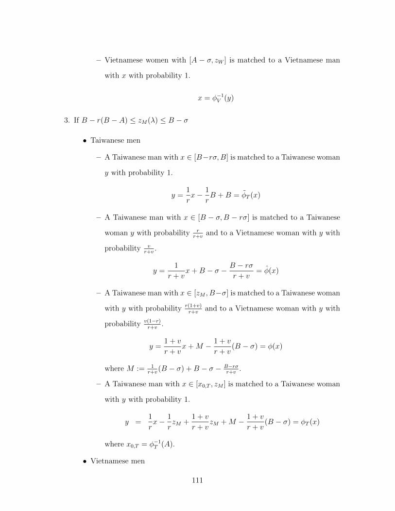
– Vietnamese women with [A − σ, zW ] is matched to a Vietnamese man


x = φ−1V (y)

3. If B − r(B − A) ≤ zM(λ) ≤ B − σ

• Taiwanese men

– A Taiwanese man with x ∈ [B−rσ,B] is matched to a Taiwanese woman


y =1

rx− 1

rB +B = φT (x)

– A Taiwanese man with x ∈ [B − σ,B − rσ] is matched to a Taiwanese



probability vr+v

.

y =1

r + vx+B − σ − B − rσ

r + v= φ(x)

– A Taiwanese man with x ∈ [zM , B−σ] is matched to a Taiwanese woman

with y with probability r(1+v)r+v


probability v(1−r)r+v

.

y =1 + v

r + vx+M − 1 + v

r + v(B − σ) = φ(x)

where M := 1r+v

(B − σ) +B − σ − B−rσr+v

.

– A Taiwanese man with x ∈ [x0,T , zM ] is matched to a Taiwanese woman


y =1

rx− 1

rzM +

1 + v

r + vzM +M − 1 + v

r + v(B − σ) = φT (x)


• Vietnamese men

111

– A Vietnamese man with x ∈ [x0,V , B − σ] is matched to a Vietnamese


y =1 + v

r + vx+M − 1 + v

r + v(B − σ) = φ(x) if x ≥ zM

y = x− zM +1 + v

r + vzM +M − 1 + v

r + v(B − σ) = φV (x) if x ≤ zM


• Taiwanese women

– A Taiwanese woman with y ∈ [A,B] is matched to a Taiwanese man


x = φ−1T (y) if y ≥ B − σ

x = φ−1(y) if M ≤ y ≤ B − σ

x = φ−1(y) if zW ≤ y ≤M

x = φ−1T (y) if A ≤ x ≤ zW

where zW := φ(zM).

• Vietnamese women

– A Vietnamese woman with [M,B − σ] is matched to a Taiwanese man


x = φ−1(y)

– A Vietnamese woman with [zW ,M ] is matched to Taiwanese man with

x with probability 1−r1+v

and Vietnamese men with [zM , B−σ] with prob-

ability r+v1+v

.

x = φ−1(y)

– Vietnamese women with [A − σ, zW ] is matched to a Vietnamese man


x = φ−1V (y)

112

4. If zM(λ) ≤ B − r(B − A)

• Same as no cost.


Proof. There are multiple ways to approach the problem. I start with a direct ap-

proach; assuming that the equilibrium is as explained in the Proposition, a complete

characterization on matching and surplus division can be obtained. Then, the stability

conditions can be verified. I show the case when zM(λ) ≤ B − σ. Other cases can be

proved in a similar way.

– Step 1 (Matching functions):

– Taiwanese men

∗ A Taiwanese man with x ∈ [B−rσ,B] is matched to a Taiwanese woman


y =1

rx− 1

rB +B = φT (x)

∗ A Taiwanese man with x ∈ [B − σ,B − rσ] is matched to a Taiwanese



probability vr+v

.

y =1

r + vx+B − σ − B − rσ

r + v= φ(x)

∗ A Taiwanese man with x ∈ [zM , B−σ] is matched to a Taiwanese woman

with y with probability r(1+v)r+v


probability v(1−r)r+v

.

y =1 + v

r + vx+M − 1 + v

r + v(B − σ) = φ(x)

where M := 1r+v

(B − σ) +B − σ − B−rσr+v

.

113

∗ A Taiwanese man with x ∈ [x0,T , zM ] is matched to a Taiwanese woman


y =1

rx− 1

rzM +

1 + v

r + vzM +M − 1 + v

r + v(B − σ) = φT (x)


– Vietnamese men

∗ A Vietnamese man with x ∈ [x0,V , B − σ] is matched to a Vietnamese


y =1 + v

r + vx+M − 1 + v

r + v(B − σ) = φ(x) if x ≥ zM

y = x− zM +1 + v

r + vzM +M − 1 + v

r + v(B − σ) = φV (x) if x ≤ zM


– Taiwanese women

∗ A Taiwanese woman with y ∈ [A,B] is matched to a Taiwanese man


x = φ−1T (y) if y ≥ B − σ

x = φ−1(y) if M ≤ y ≤ B − σ

x = φ−1(y) if zW ≤ y ≤M

x = φ−1T (y) if A ≤ x ≤ zW

where zW := φ(zM).

– Vietnamese women

∗ A Vietnamese woman with [M,B − σ] is matched to a Taiwanese man


x = φ−1(y)

114

∗ A Vietnamese woman with [zW ,M ] is matched to Taiwanese man with

x with probability 1−r1+v

and Vietnamese men with [zM , B−σ] with prob-

ability r+v1+v

.

x = φ−1(y)

∗ Vietnamese women with [A − σ, zW ] is matched to a Vietnamese man


x = φ−1V (y)

– Step 2 (Individual utilities):

– Taiwanese men

uT (x) =

uT (x), if B − rσ ≤ x ≤ B

uT (x), if B − σ ≤ x ≤ B − rσ

uT (x), if zM ≤ x ≤ B − σ

uT (x), if x0,T ≤ x ≤ zM

0, if x ≤ x0,T

– Vietnamese men

uV (x) =

uV (x), if zM ≤ x ≤ B − σ

uV (x), if x0,V ≤ x ≤ zM

0, if x ≤ x0,V

115

– Taiwanese women

vT (x) =

vT (y), if B − σ ≤ y ≤ B

vT (y), if M ≤ y ≤ B − σ

vT (y), if zW ≤ y ≤M

vT (y), if A ≤ y ≤ zW

– Vietnamese women

vV (x) =

vV (y), if M ≤ y ≤ B − σ

vV (y), if zW ≤ y ≤M

vV (y), if A− σ ≤ y ≤ zW

where

116

u′T (x) = Sx(x, φ(x))

uT (x) =

∫ x

B−rσSx(s, φ(s))ds+ P

u′T (x) = Sx(x, φ(x))

uT (x) =

∫ x

B−σSx(s, φ(s))ds+Q

u′T (x) = Sx(x, φ(x))

uT (x) =

∫ x

zM

Sx(s, φ(s))ds+R

u′T (x) = Sx(x, φT (x))

uT (x) =

∫ x

x0,T

Sx(s, φT (s))ds+ S

u′V (x) = Sx(x, φ(x))

uV (x) =

∫ x

zM

Sx(s, φ(s))ds+R′

u′V (x) = Sx(x, φ(x))

uV (x) =

∫ x

x0,V

Sx(s, φV (s))ds+ S ′

v′T (y) = Sy(φ−1(y), y)

vT (y) =

∫ y

B−σSy(φ

−1(t), t)dt+ J

v′T (y) = Sy(φ−1(y), y)

vT (y) =

∫ y

M

Sy(φ−1(t), t)dt+K

v′T (y) = Sy(φ−1(y), y)

vT (y) =

∫ y

zW

Sy(φ−1(t), t)dt+ L

v′T (y) = Sy(φ−1T (y), y)

vT (y) =

∫ y

a

Sy(φ−1T (t), t)dt+O

v′V (y) = Sy(φ−1(y), y)

vV (y) =

∫ y

M

Sy(φ−1(t), t)dt+K ′

v′V (y) = Sy(φ−1(y), y)

vV (y) =

∫ y

zW

Sy(φ−1(t), t)dt+ L′

v′V (y) = Sy(φ−1V (y), y)

vV (y) =

∫ y

a

Sy(φ−1V (t), t)dt+O′

117

– The constants are:

S = 0

S ′ = 0

R =

∫ zM

x0,T

Sx(s, φT (s))ds

R′ =

∫ zM

x0,V

Sx(s, φV (s))ds

Q =

∫ B−σ

zM

Sx(s, φ(s))ds+

∫ zM

x0,T

Sx(s, φT (s))ds

P =

∫ B−rσ

B−σSx(s, φ(s))ds+

∫ B−σ

zM

Sx(s, φ(s))ds+

∫ zM

x0,T

Sx(s, φT (s))ds

O = S(x0,T , A)

O′ = S(x0,V , A− σ)

L =

∫ zW

A

Sy(φ−1T (t), t)dt+ S(x0,T , A)

L′ =

∫ zW

A−σSy(φ

−1V (t), t)dt+ S(x0,V , A− σ)

K =

∫ M

zW

Sy(φ−1(t), t)dt+

∫ zW

A


K ′ =

∫ M

zW

Sy(φ−1(t), t)dt+

∫ zW

A−σSy(φ

−1V (t), t)dt+ S(x0,V , A− σ)

J =

∫ B−σ

M

Sy(φ−1(t), t)dt+

∫ M

zW

Sy(φ−1(t), t)dt

+

∫ zW

A


First two are zero because the last married men should be indifferent with

being single. Accordingly, the lowest type women exploit all the surplus

generated from the marriage. The rest follows from the continuity of utilities.

– Step 3 (Finding zM and zW ): From Proposition 2, we have uT (x) + λ = uV (x).

Thus, R + λ = R′ and zM can be found. zW can be found by plugging zM in

zW = φ(zM).

118

– Step 4 (Verifying stability conditions): The stability conditions need to be ver-

ified for all possible couples. There are 72 possible pairs (uT , uT , uT , uT , uV ,

uV , Taiwanese single, Vietnamese single for men and vT , vT , vT , vT , vV , vV ,

vV for women). Among those, the pairs who marry with positive probability

in the equilibrium (8 cases) satisfy the stability condition because within cate-

gories, male and female match positive assortatively from Proposition 1 (under

supermodularity, such match is stable). Note that S(x, y) = xy.

– uT and vV :

We need to check

P (x, y) = uT (x) + vV (y)− S(x, y) + λ ≥ 0

for x0,T ≤ x ≤ zM and A− σ ≤ y ≤ zW . P (x, y) can be rewritten as

P (x, y) =

∫ x

x0,T

Sx(s, φT (s))ds+ S +

∫ y

A−σSy(φ

−1V (t), t)dt+O′ − xy + λ ≥ 0

This gives Pxx = φ′T (x) = 1r, Pyy = φ−1′

V (y) = 1, and Pxy = −1. Thus,

P (x, y) is convex in (x, y) and its minimum satisfies

∂P (x, y)

∂x=∂P (x, y)

∂y= 0

Sx(x, φT (x))− Sx(x, y) = 0

Sy(φ−1V (y), y)− Sy(x, y) = 0

To satisfy both conditions, the following should be the case: y = φT (x) and

y = φV (x). This happens at the cutoff x = zM . Note that vV (zW ) + λ =

vT (zW ). P (zM , zW ) = uT (zM) + vV (zW )− S(x, y) + λ = uT (zM) + vT (zW )−

S(x, y) = 0, so the condition is satisfied.

119

– uT and vV :

We need to check

P (x, y) = uT (x) + vV (y)− S(x, y) + λ ≥ 0

for x0,T ≤ x ≤ zM and zW ≤ y ≤ M . Since we know P (zM , zW ) = 0, if

P (x, y) is decreasing in x and increasing in y, P (x, y) in all (x, y) in the

ranges. This can be shown as follows:

∂P (x, y)

∂x= φT (x)− y ≤ 0

∂P (x, y)

∂y= φ−1(y)− x ≥ 0.

For the remaining cases as well, using similar computations, it can be shown that

the difference u + v − Σ between the sum of individual utilities and potential

surplus is minimum at the boundary or at some non-negative interior point. The

explicit calculations are available upon request.


Proof. – ∂zM∂λ

> 0:

This can be proved by using the Leibniz integral rule.

λ = R′ −R

=

∫ zM

x0,V

Sx(s, φV (s))ds−∫ zM

x0,T

Sx(s, φT (s))ds

=

∫ zM

A−σ+ r−1r+v

zM−M+ 1+vr+v

(B−σ)Sx(s, s− zM +

1 + v

r + vzM +M − 1 + v

r + v(B − σ))ds

−∫ zM

rA+v(1−r)r+v

zM−M+ 1+vr+v

(B−σ)Sx(s,

1

rs− 1

rzM +

1 + v

r + vzM +M − 1 + v

r + v(B − σ))ds

120

Using the Leibniz integral rule,

∂λ

∂zM= Sx(zM , zW ) + Sx(A− σ +

r − 1

r + vzM −M +

1 + v

r + v(B − σ), A− σ)

1− rr + v

+

∫ zM

A−σ+ r−1r+v zM−M+ 1+v

r+v (B−σ)Sxy(s, s− zM +

1 + v

r + vzM +M − 1 + v

r + v(B − σ))

1− rr + v

ds

−Sx(zM , zW ) + Sx(rA+v(1− r)r + v

zM −M +1 + v

r + v(B − σ), A)

1− rr + v

v

+

∫ zM

rA+v(1−r)r+v zM−M+ 1+v

r+v (B−σ)Sxy(s,

1

rs− 1

rzM +

1 + v

r + vzM +M − 1 + v

r + v(B − σ))

v(1− r)r(r + v)

ds

> 0

because Sxy > 0. Thus, we have ∂zM∂λ

> 0.

– ∂zW∂λ

> 0:

zM = φ(zW ) and φ′(x) > 0. From ∂zM∂λ

> 0, ∂zW∂λ

> 0.

– ∂φT (x)∂λ

< 0

Note that φT (x) = 1rx − 1

rzM + 1+v

r+vzM + M − 1+v

r+v(B − σ). Given x, ∂φT (x)

∂zM=

v(r−1)r(r+v)

< 0. From ∂φT (x)∂λ

= ∂φT (x)∂zM

∂zM∂λ

, the result follows.

– ∂φV (x)∂λ

> 0

Note that φV (x) = x − zM + 1+vr+v

zM + M − 1+vr+v

(B − σ). Given x, ∂φV (x)∂zM

=

−1 + 1+vr+v

> 0. From ∂φV (x)∂λ

= ∂φV (x)∂zM

∂zM∂λ

, the result follows.

–∂x0,T∂λ

> 0

Note that x0,T = φ−1T (A) = rA + v(1−r)

r+vzM −M + 1+v

r+v(B − σ). Using the chain

rule, the result follows.

–∂x0,V∂λ

< 0

Note that x0,V = φ−1V (A − σ) = A − σ + r−1

r+vzM −M + 1+v

r+v(B − σ). Using the

121

chain rule, the result follows.

– ∂uT (x)∂λ

< 0

Use the Leibniz integral rule to show ∂uT (x)∂zM

< 0. Then use the chain rule.

– ∂uV (x)∂λ

> 0

Use the Leibniz integral rule to show ∂uV (x)∂zM

> 0. Then use the chain rule.

– ∂vT (y)∂λ

> 0

Use the Leibniz integral rule to show ∂vT (y)∂zM

> 0. Then use the chain rule.

– ∂vV (y)∂λ

< 0

Use the Leibniz integral rule to show ∂vT (y)∂zM

< 0. Then use the chain rule.

A.6 Multiplicative Cost Case

This subsection provides the theoretical results when cost varies with the surplus. These

results can be obtained with a minor modification to the surplus function given in

Chiappori et al. (2017). Assume the same population structures given in 3.1.1. Suppose

the surplus function is given as follows:

ΣXY (x, y) =

S(x, y), if X = Y

(1− λ)S(x, y), if X 6= Y

where λ < 1. The function S is strictly increasing, continuously differentiable, and

supermodular. Normalize single utility as 0 and assume that S(0, 0) ≥ 0.

122

Proposition 6. In the stable matching, if (x,X) and (x′, X) such that x ≥ x′ are

matched to (y, Y ) and (y′, Y ), respectively, y ≥ y′ almost surely.

Proof. Suppose x ≥ x′ but y′ > y with a positive measure. The surplus is:

Σ1 = ΣXY (x, y) + ΣXY (x′, y′)

By switching the couples, the surplus becomes

Σ2 = ΣXY (x, y′) + ΣXY (x′, y) > Σ1

by supermodularity. It contradicts to surplus maximization.

Note that under the multiplicative cost case, the matching is positive assortative

on SES within same categories of men and women. The positive assortative matching

results under the fixed cost case is stronger because a stable matching is positive assor-

tative on SES when holding one gender’s country and considering the two countries for

the other gender. This result does not hold anymore under multiplicative cost because

the cost depends on the types of the agents.

Proposition 7. Suppose an open set of males from X country are indifferent be-

tween marrying a woman from T country and a woman from V country so that 0 <

p(T |x,X) < 1 in the stable match for any x in the open set. If (x,X) is matched to

either (y, T ) or (y′, V ), then y < y′ if X = T and y > y′ if X = V .

Similarly, suppose an open set of females from Y country are indifferent between

marrying a man from T country and a man from V country so that 0 < q(X|y, Y ) < 1

in the stable match for any y in the open set. If (y, Y ) is matched to either (x, T ) or

(x′, V ), then x < x′ if Y = T and x > x′ if Y = V .

Proof. Let X be T . Suppose a man x from country T is matched to either a woman y

from country T or a woman y′ from country V at the stable match. Let uT (x) be his

123

utility. Then, by stability,

uT (x) = maxs

(S(x, s)− vT (s))

= maxs′

(λS(x, s′)− vV (s′))

where vT (s) (vV (s′)) is the utility of a woman from country T (a woman from country

V ) with the type s (s′); note that the maximum is reached at s = y and s′ = y′

respectively. By the envelope theorem:

u′T (x) =∂

∂xS(x, y) = λ

∂

∂xS(x, y′)

Since ∂S∂x

is strictly increasing in y and λ < 1, y < y′. The remainder can be proved

similarly.

Note that unlike the fixed cost case where the types of spouses from different coun-

tries are same, with the multiplicative cost, the type of spouse from the different country

should be higher than that from the same country. If the spouse is from the different

country, the part of the surplus that generates complementarities decreases unlike the

fixed cost case. That loss of the surplus is compensated by the higher type of the spouse

from the different country.

Proposition 8. Assume that there exists an open set O such that for all (x,X) where

x ∈ O, 0 < p(T |x,X) < 1. That is, (x,X) marries either a woman (y, T ) or (y, V ) with

positive probability. Then, q(X|y,X) = 0 for almost surely where {X} = {T, V }−{X}.

Similarly, assume that there exists an open set O′ such that for all (y, Y ) where

y ∈ O′, 0 < q(T |y, Y ) < 1. That is, (y, Y ) marries either a woman (x, T ) or (x, V ) with

positive probability. Then, p(Y |y, Y ) = 0 for almost surely where {Y } = {T, V }−{Y }.

Proof. Without loss of generality, let X = T . Suppose q(V |y, T ) > 0 on a set with

positive measure. That is, (y, T ) is matched to either (x, T ) and (x′, V ) with x′ > x.

124

Since we have 0 < p(T |x, T ) < 1, (x, T ) is matched to either (y, T ) or (y′, V ) with

y′ > y. The surplus generated from (x, T ), (y′, V ) couple and (x′, V ), (y, T ) couple is

Σ1 = λS(x, y′) + λS(x′, y)

By switching the surplus is

Σ2 = S(x, y) + S(x′, y′) > Σ1

since x′ > x and y′ > y. The rest can be proved similarly.

The result on the one-sided randomization holds under both fixed cost case and

multiplicative cost case. In a given neighborhood, two types of randomization cannot

happen at the same time. For instance, if Taiwanese women marry cross-nationally, it

must be the case that Taiwanese men marry only Taiwanese women in that neighbor-

hood.

125

Figure A.1: Comparative statics with respect to cost of cross-border marriages (λ1 < λ2)

A. Taiwanese Men B. Vietnamese Men C. Taiwanese Women D. Vietnamese Women

Single probability

0.00

0.25

0.50

0.75

1.00

Α Β − σ Β

Prob. of marrying a Taiwanese

0.00

0.25

0.50

0.75

1.00

Α Β − σ Β

Prob. of marrying a Vietnamese

0.00

0.25

0.50

0.75

1.00

Α Β − σ Β

Matching functions

Α − σ

Α

Β − σ

Β

Α Β − σ Β

SE

S o

f Spo

uses

Individual utilities

0

5

10

15

20

Α Β − σ Β

Socioeconomic status of Taiwanese men

u T(x

)

Single probability

0.00

0.25

0.50

0.75

1.00

Α − σ Α Β − σ


0.00

0.25

0.50

0.75

1.00

Α − σ Α Β − σ


0.00

0.25

0.50

0.75

1.00

Α − σ Α Β − σ

Matching functions

Α − σ

Α

Β − σ

Β

Α − σ Α Β − σ

SE

S o

f Spo

uses


0

5

10

15

20

Α − σ Α Β − σ

Socioeconomic status of Vietnamese men

u V(x

)

Single probability

0.00

0.25

0.50

0.75

1.00

Α Β − σ Β


0.00

0.25

0.50

0.75

1.00

Α Β − σ Β


0.00

0.25

0.50

0.75

1.00

Α Β − σ Β

Matching functions

Α − σ

Α

Β − σ

Β

Α Β − σ Β

SE

S o

f Spo

uses


0

5

10

15

20

Α Β − σ Β

Socioeconomic status of Taiwanese women

v T(y

)

Single probability

0.00

0.25

0.50

0.75

1.00

Α − σ Α Β − σ


0.00

0.25

0.50

0.75

1.00

Α − σ Α Β − σ


0.00

0.25

0.50

0.75

1.00

Α − σ Α Β − σ

Matching functions

Α − σ

Α

Β − σ

Β

Α − σ Α Β − σ

SE

S o

f Spo

uses


0

5

10

15

20

Α − σ Α Β − σ

Socioeconomic status of Vietnamese women

v V(y

)

λ1λ2

Notes: These figures plot comparative statics results. For these illustrative figures, the parameter values A = 2, B = 6, σ = 1.4, r = 0.7,v = 2, λ1 = 2.2 and λ2 = 3 are used. The grey lines on matching graphs indicate y = x. MATLAB codes are available upon request.

126

Appendix B

Appendix to Chapter 2

127

B.1 Intra-Household Allocation Results in Taiwan

B.1.1 Data

For intra-household outcomes, I use the Panel Survey of Family Dynamics (PSFD). The

PSFD includes two variables that I use as intra-household outcomes; it contains first,

the information on weekly hours spent on household works and second, yearly clothing

expenditure of the respondents and their spouses. It also surveys the year of marriage,

which allows me to evaluate the impact of changes in visa policies on the relative status

of women within households. I use 2007 data only because that is the only year when

the survey collected information on spending for both husbands and wives.

B.1.2 Impact on intra-household allocations

Prediction 5. When the cost of cross-border marriage increases, the power within

households for wives improves whereas the power of husbands decreases in Taiwan.

For marriage rates and matching patterns, the changes in costs of cross-border

marriage affect only a subset of populations. However, one of the powerful results in

matching literature is that once market condition changes, the share within marriage

for everyone changes. In the specific case of the visa tightening policy, the individual

utilities of women increases for all women and the individual utilities of men decreases

for all men. Thus, albeit interesting, it is difficult to test this prediction compared

to marriage rates or matching patterns because there does not exist a natural control

group. Instead, I compare men and women in terms of measures of bargaining power

within households, which is proxied by weekly hours on household work and individual

spending on clothing. Since the model predicts that the power of wives increases and

that of husbands decreases, we would expect to see that the time spent on household

work for husbands increases compared to for the wives and the spending on clothing of

128

husbands decreases compared to that of wives.

Yigy = βfemaleg × Posty + γg + δy + νXi + εigy

where i is an individual, g is gender, and y is the year of marriage. The controls

include the ages of husbands and wives, and district fixed effects. For the spending on

clothing, I also control for total expenditure of the household in the form of the product

of level and log level in the spirit of Working-Leser model. This allows differential impact

of total expenditure by its level.

The results are presented in Table B.1. The results show that the weekly hours of

household work decreases and the spending on clothing increases for wives compared

to the husbands after the visa tightening policy although the result on spending on

clothing is not significant. This suggests that the power of women within households

is enhanced when it becomes more difficult for Vietnamese women to enter Taiwan,

which is consistent with the theoretical prediction.

129

Table B.1: The impact of visa tightening policies on intra-household allocations in Taiwan

Dep. var.: HH work (hours per week) Yearly clothing spending (NTD)

(1) (2) (3) (4) (5) (6)

Female X Post -5.00∗∗∗ -4.98∗∗∗ -2.95 546.6 669.2 410.1(1.72) (1.62) (1.91) (1011.8) (864.9) (996.5)

Controls No Yes Yes Yes Yes Yes

Gender trend No No Yes Yes Yes Yes

Dep. var. mean (male) 4.79 4.79 4.79 4580.14 4580.14 4580.14

Dep. var. mean (female) 14.35 14.35 14.35 7234.55 7234.55 7234.55

R-squared 0.247 0.330 0.331 0.092 0.375 0.375

Observations 3,034 3,032 3,032 2,017 2,015 2,015

Notes: This table shows the results from regression in subsection B.1.2. Control variables include the education of husband, educationof wife, age of husband, age of wife and dummies for district. For spending on clothing, I also control for total expenditure multipliedby log total expenditure in the spirit of Working-Leser specification. Robust standard errors are used. Significance levels: * 10%, **5%, *** 1%. Source: Panel Survey of Family Dynamics 2007. Only Taiwanese couples who married in 1970 and after are used assamples.

130

B.2 Proportionality Test Results

Table B.2: Proportionality test results

Tbc exp. JWM exp.

Intensity of cross-border marriages -2.96** 2.69***

(1.31) (0.85)

Intensity of male-intensive agriculture 0.0086** -0.0050**

(0.0035) (0.0023)

Proportionality test p=0.5885

N 18,520 18,520

Notes: This table shows the results of the proportionality tests for the collective model. Intensity ofcross-border marriages and intensity of male-intensive agriculture are used as two distribution factors.

131

B.3 Additional Figures

Figure B.1: Probability of marrying cross-nationally conditional on education (Tai-wanese men)

0.0

05.0

1.0

15.0

2.0

25

shar

e

Less than primary Primary Junior High Senior High College/Univ. Grad. degree

Notes: This figure plots probability of marrying cross-nationally conditional on education.

Figure B.2: Probability of marrying cross-nationally conditional on education (Viet-namese women)

0.0

2.0

4.0

6.0

8

shar

e


Notes: This figure plots probability of marrying cross-nationally conditional on education.

132

Figure B.3: Prevalence of ultrasound technologies in rural Vietnam

0.2

.4.6

.81

Rat

e of

mot

hers

kno

win

g th

e se

x by

ultr

asou

nd

2005 2006 2007 2009 2010 2011 2012 2013

Affected Provinces Unaffected Provinces

Notes: This figure plots the sex ratios at birth in the provinces that were initially affected by cross-border marriages and the rest of the provinces. The provinces with more than 1% of women out-migrated in 2003 were classified as the affected provinces. Sources: the Vietnamese census 1999 and2009.

133

matching in marriage market and labor market

Documents