mathematical biosciences 499 application of the ... of the... · mathematical biosciences 499...

MATHEMATICAL BIOSCIENCES 499

Application of the Mathematical Theory of Sequential Sampling to Gamma Scanning in Nuclear Medicine

HENRY S. KATZENSTEIN Solid State Radiations, Inc.,* Los Angeles, California

LEONARD KLEINROCK Solid State Radiations, Inc., Los Angeles, and Department of Engineering, University of

California, Los Angeles, California

ALLEN STUBBERUD Solid State Radiations, Inc., Los Angeles, and Department of Engineering, University of

California, Los Angeles, California

AND

STEPHEN S. FRIEDLAND Department of Medicine, ** University of Southern California, Los Angeles,

Department of Physics, Sun Fernando Valley State College, Northridge, California

Communicated by Richard Bellman

and

ABSTRACT

To minimize the time for performing a gamma scan in nuclear medicine, optimum use must be made of the statistical data from the scan to control the time of observation at any given point. In the work described, the sequential sampling technique has been applied to the problem of proportioning observation time on the basis of observed counts. In the limit of both very high and very low count rates, advantage is taken of the rapid decision time afforded by the good statistics of high rates and the a priori rejection of areas exhibiting low rates. Areas of intermediate activity require longer times to obtain a statistically significant estimate of activity. In this scanning method, accumulated counts from a stationary sensor are compared with two (linearly) time- varying thresholds: upon crossing either threshold an intensity estimate is made (which may be binary) and the scan continued to the next point. This procedure is well known in sequential hypothesis testing and the theory developed is pertinent to the gamma scanning application. An analysis of the system as compared to a fixed observation-time-in-scanning has been made. For a two-level detection system, with a given error probability and a given ratio of decay rate for a high-activity region to that for a low-activity region, it has been found that the average observation time for a variable threshold scanning is approximately half that for fixed-time scanning.

* Supported by the Division of Biology and Medicine, U.S. Atomic Energy Com- mission under contract AT@&3)-627.

** Supported by the National Institutes of Health under grant no. GM-14633-02.

Mathematical Biosciences 4 (1969), 499-530

Copyright 0 1969 by American Elsevier Publishing Company, Inc.

HENRY S. KATZENSTEIN et al.

1. INTRODUCTION

Many types of tumors can be detected by a measurement of the rate of

radioisotope uptake (after an injection of a radioisotope tracer into the

bloodstream), the rate being greater in the tumorous growth as compared

to the surrounding normal tissue. A complete understanding of the

mechanism of the selective pickup of a particular labeled molecule in any

given tumor is not understood. Suffice to say for this writing that selective

pickups in many types of brain tumors, eye lesions, and so on do occur,

and that their presence in the tumor, after a predetermined time interval

following the injection of the radioisotope, is positive indication of a

malignancy. The location and geometrical distribution of the radioisotope

pickup furnish definitive information concerning the nature, extent, and

condition of any abnormality.

If a beta-emitting isotope is employed, such as P32, it is necessary to

insert a nuclear radiation detector in or near the tumor to determine the

relative concentration of the isotope. This is because beta particles have

a short range, several millimeters, in tissue. If information on the spatial

distribution of the beta-emitting isotope is to be obtained, then the probe

position must be inserted into the patient and transported throughout the

volume of interest while plotting the relative concentration. Such a

surgical procedure is only possible in a limited number of cases and is

rarely desirable.

If a gamma-emitting isotope is used, the detector may be placed outside

the body, thus removing the need for surgical implementation. However,

the use of collimators and other data-handling devices are required to

determine the nature and the source of the radiation.

These methods of tumor localization have been under investigation

and development for the past two decades. For brain tumor detection,

the methods may utilize P32, Ir31, Hg203, and other isotopes, which are

selectively absorbed because of the disruption of the normal blood flow

through the blood brain barrier.

Gamma Scanning

Gamma scanning is a method of visualizing the distribution of radio-

active tracers, which have been selectively absorbed by the tumor, to

assist in the visualization of the growth, so that more accurate diagnostic

evaluation for treatment may be made. As an example of scanning,


GAMMA SCANNING IN NUCLEAR MEDICINE 501

consider a study of the condition of the thyroid gland and the I13i uptake

in the gland tissue. Although this is not strictly a tumor localization

problem, the techniques and methods are identical.

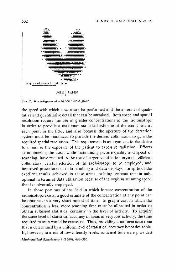
As described by Blahd [l], the normal thyroid gland has a “butterfly”

appearance. It weighs approximately 20 gm and its right lobe is usually

larger than its left. The lobes are interconnected by an isthmus, but in

some instances the isthmus may be entirely absent. In a patient suffering

Suprasternal notch

MID

RIGHT I LINE

LEFT

FIG. 1. A scintigram of the normal thyroid.

with hyperthyroidism the thyroid gland may be three or four times its

normal size and its specific location is diffused. Figure 1 is a scintigram

(i.e., the two-dimensional plot of the gamma scan) of the normal thyroid

gland and Fig. 2 is a scintigram of a hyperthyroid gland. Each dot on the

scintigram represents a given number of radiation counts in a collimated

radiation detector. In those areas where the density of points is high, the

nuclear radiation level is correspondingly high. Clearly, from such thyroid

scintigrams, the physical size, location, and distribution of the thyroid

gland may be ascertained. Thyroid nodules are quite common and are

observed on scintigrams as rarified or nonfunctioning areas. Their

existence usually denotes thyroid cancer, which means that they must be

examined with care. Numerous other patterns of iodine uptake in the

thyroid gland and elsewhere in the body are known that bear a one-to-one

correspondence with human disorders.

Although the technique of scanning has been thoroughly established

in the practice of nuclear medicine, limitations have arisen with regard to


502 HENRY S. KATZENSTEIN et al.

C.. . . . I=. . .._. ._ . . . .= ..- ._.‘. . . . *. :... . 2tzz.. . ..-. -.. .._-.. . .-.* z.. . ..v.. .- . a.-.. . -.-.. . .;. -. . . . in.. . . .-. -*. . . *- : ._,p_ ,” . .Z’ . ‘.

-. . . . . . . . . . . . .

. * . . - “.. _, ;- . . -_ ..B._: .- .._ . .- . ._ c*. *

Suprasternal notch

MID LINE I

FIG. 2. A scintigram of a hyperthyroid gland.

the speed with which a scan can be performed and the amount of quali-

tative and quantitative detail that can be surmised. Both speed and spatial

resolution require the use of greater concentrations of the radioisotope

in order to provide a maximum statistical estimate of the count rate at

each point in the field, and also because the aperture of the detection

system must be minimized to provide the desired collimation to gain the

required spatial resolution. This requirement is antagonistic to the desire

to minimize the exposure of the patient to excessive radiation. Efforts

at minimizing the dose, while maintaining picture quality and speed of

scanning, have resulted in the use of larger scintillation crystals, efficient

collimators, careful selection of the radioisotope to be employed, and

improved procedures of data handling and data displays. In spite of the

excellent results achieved in these areas, existing systems remain sub-

optimal in terms of data utilization because of the uniform scanning speed

that is universally employed.

In those portions of the field in which intense concentration of the

radioisotope exists, a good estimate of the concentration at any point can

be obtained in a very short period of time. In gray areas, in which the

concentration is less, more scanning time must be allocated in order to

obtain sufficient statistical certainty in the level of activity. To acquire

the same level of statistical accuracy in areas of very low activity, the time

required to scan would be excessive. Thus, providing a uniform scan time

that is determined by a uniform level of statistical accuracy is not desirable.

If, however, in areas of low intensity levels, sufficient time were provided

MathematicaI Biosciences 4 (1969), 499-530


to establish that a low-level intensity level indeed exists at one point,

before passing on to the next point in the field, the scan procedure could

be improved by reducing the scan time. This procedure has been for-

malized in the mathematical theory of sequential sampling and has been

applied successfully to problems of radar search, optimum sampling

procedures for quality control, and other similar problems. Let us

consider some of these applications to attain a better feel of the nature of

the theory of sequential sampling before applying it to the subject at

hand.

Qualitatioe Descriptiorz of the Application of the Theory of Sequential

Sampling

Quality Control Problem

In the quality control problem, by which we attempt to evaluate the

properties of a large population by withdrawing samples and testing them,

it is clearly desirable to use a minimum number of samples, both to

minimize the amount of testing that must be done and to conserve the

product being evaluated, since the testing process is frequently destructive.

The proper sample size depends on the desired degree of confirmation of a

given property of the population. As the requirement for assurance

increases, the size of the test lot similarly increases, to the point where all

units must be subjected to the test. If the test should be destructive, this

is clearly catastrophic and impractical. For this reason, a process of

sampling is adopted in which the size of the sample is adjusted for the

desired degree of confirmation from an estimation of results obtained.

For example, a lot of ten units may be tested. If no defective unit is

found, a degree of confirmation of the quality of the population can be

affirmed. If a certain number, say two, of these units tested are found to

be defective, the lot can be rejected without further testing. However, a

third alternative exists. If only one defective unit is discovered, the alter-

native is to take another sample of, for example, ten units; since one

defective unit in ten may not in this case convey sufficient information to

warrant either accepting or rejecting the lot. The essence of sequential

sampling is that each trial results in three, rather than two, possible

alternatives. These are (1) accept; (2) reject; or (3) take another sample.

In some quality control instances, the adoption of this method has resulted

in a reduction, by a factor of ten, in the number of units tested to obtain a

given degree of confirmation concerning the lot as a whole.



Radar Scanning

In the radar scanning problem, the same principle is involved. If an

antenna scans at a fast rate, targets will be lost or false alarms generated

due to the insufficient time on target to integrate the echo to a value

sufficiently above the noise. On the other hand, a scan that is excessively

slow will permit fast-moving objects to pass out of the range of the radar

without ever being detected. If it is necessary to choose a single scanning

rate, we must choose an intermediate compromise that permits some lost

targets from both lack of sufficient time on target or too much delay in

scanning a given portion of the field. If, however, we scan in accordance

with sequential sampling techniques, it is possible to enhance the target-

detecting efficiency of the radar. The procedure is similar to the quality

control problem. The radar antenna looks at a particular volume of

space and integrates the signal obtained over a given period of time. If

the integrated echo signal fails to exceed a certain threshold, the output is

indicated as “no target” and the antenna moves on to another volume.

On the other hand, if the signal exceeds a second threshold, which is

higher, the volume of space is indicated as containing a target and again

the antenna moves on to another volume. For those cases where the

signals fail to cross either threshold, the antenna remains stationary until

the integration process causes the signal level to cross either the upper or

lower threshold. Thus again, a three-level decision is made: (1) yes,

there is a target in the beam; (2) no, there is not a target in the beam;

or (3) there is not sufficient information to make a decision, and therefore

it is necessary to continue to observe.

Radioiscope Scanning

The application of this technique to the scanning of a gamma-emitting

isotope is now clear. The detector is positioned at the first point to be

observed and the counting rate applied to a three-level (two-threshold)

system. If the counting rate is below a certain threshold, the detector is

moved since this area can definitely be regarded as background. If the

counting rate exceeds a higher threshold, the detector can likewise be

moved to another position since the statistics accumulated are adequate

to permit us to decide that an “intense” level exists. If neither of these

thresholds is crossed, the detector remains stationary until sufficient

statistics can be accumulated to enable us to estimate the intensity level of

that area to the required accuracy; thus, the majority of the scanning time



is occupied in scanning the transition areas between intense and back-

ground levels in an attempt to obtain better information where an imme-

diate decision concerning the intensity cannot be inferred. The precise

setting of the threshold levels and the criteria for proper statistics will,

of course, be determined by a detailed study of the nature of the lesions,

tumors, gland, and so forth being observed with some a priori knowledge

concerning the types of patterns expected. Thus, these thresholds can be

set to yield the maximum amount of information for the least scanning

time.

2. THE MODEL

In order to analyze the performance of the proposed scanning method,

it is necessary to formulate a precise mathematical model of the radio-

active source. Once this is accomplished, any completely defined scheme

for sampling the source can be evaluated and compared to other proposed

schemes on the basis of their relative performance.

Given a two-dimensional radioactive area that must be scanned, at

any position (x, 1)) of this area there exists a radiation decay whose average

number of counts per second is 2(x, y). It is assumed that the half life

of the source of this radiation is significantly longer than the duration of

any scanning method it is proposed to analyze. It is well known [2, 31

that a radioactive decay source is accurately represented by a Poisson

process with stationary independent increments. (The stationarity here

comes from the assumption of the long half life to scanning time ratio.)

This representation allows us to state that the probability P(n, r) that the

source at position (x, _y) generates n decays in a time interval of T seconds

is

P(n, T) = vr exp(-A(.u, y)T). n.

Thus the expected number of counts in T seconds is just A(.x, y)T.

The purpose of any scanning procedure is to determine the continuous

two-dimensional intensity function 2(x, v). This, however, is overly

ambitious and it usually suffices to present an array of values of 2(x, y)

at the NM points (x,,y,) where x, takes on the values xi, x2, . . . , _Y.\ and ynz takes on the values y,,y2, . . . ,yAtf. We are then faced with the

problem of devising methods for finding A(xn, y,). In Section 3, a

number of such methods are described, and in Sections 4 and 5 they are

compared to the performance of the more interesting of these. It is

31

Matl~enzatical Biosciences 4 (1969), 499-530


recognized that jl(x,, y,) (hereafter referred to as il for convenience) can

take on a continuum of values; clearly, it is sufficient for any practical

purpose to quantize this continuum into a discrete set of L allowable

values ii,, jl,, . . . , ii, where ii, < AZ < . . . < I,. Such a quantized

system is referred to as a multilevel scanning system (indeed, an L-ary

system). In order to present the results of an L-ary scanning system,

we may print one of L gray levels at each point (x,, y,) on a two-dimen-

sional plot. In order to determine the exact gray level at any point, a

fairly careful measurement of 1, must be made at each point if L is

reasonably large; this then involves a fairly long scanning time per point.

On the other hand, if L is rather small, the accuracy of representation

of 1 will be less, but so also will be the required scan time. Indeed, if L

is taken to be L = 2, the crudest possible quantization is obtained, as

well as the shortest scan time per point; such a system is referred to as

a hinary scanning system. In the binary case, only black and white

coloring appears at each point; however, the two-dimensional function

1(x,, y,) will nevertheless appear to take on gray tones due to the varying

density of black points, not unlike the gray levels that are produced in

newspapers using halftone photographs. The quality of a picture pro-

duced with a binary scanning system can be made rather high by increasing

the density of points looked at (i.e., by increasing N and M); in so doing,

of course, we pay the price of increasing the total scan time. In Section 3

various multilevel and binary (L = 2) scanning systems are described and

their relative advantages and disadvantages discussed.

Because of the essential simplicity of the mathematics and implemen-

tation of a binary scanning method, an analysis of the system with L = 2

will be made. In Section 4, an analysis of a binary fixed-time scanning

system is carried out, and a binary threshold scanning system is analyzed

in Section 5. The model in both of these systems is that of a binary source,

which is now to be described.

The binary system L = 2 quantizes all possible radiation intensities J.

into two allowed levels 2, and 2, (2, < 1,). Specifically, as shown in Fig.

3, the quantizer output is A1 for all input radiation intensities il < R,

and the output is ;i, for all I > i, where L, is the critical input intensity.

An extensive theory of sequential hypothesis testing has been developed

[5] that is applicable to the problem at hand. The assumption usually

made in that theory is that one of two mutually exclusive hypotheses HI

or Hz is true. The goal is to sample the process being tested until a

sufficiently reliable estimate is obtained as to which of the hypotheses is

Mathenzafical Biosciences 4 (1969), 499-530


Output intensity level

5

0 x Input radiation level h

FIG. 3. Binary quantizer.

true. Applying this theory to our problem, it is seen that a suitable prob-

lem formulation is one in which it is assumed that each radiation intensity

A(x,, y,) can take on only one of two values, ;1, or &; that is, the

hypotheses are HI and H, where

H, is the hypothesis that 1 = il,,

H, is the hypothesis that 1 = &.

Observe that the binary quantizer model is distinctly different from this

two-hypothesis model in that the latter allows 1, to take on only one of two

levels (2, or 2,) and the former allows 1 to take on a continuum of levels

and then maps (quantizes) this continuum into one of two levels. The

two-hypothesis theory is so appealing in its mathematical tractability,

however, that it is advisable to accept it for this analysis, recognizing that

it is only a gross simplification of the true state of affairs. Nevertheless,

it is felt that the adoption of such a model allows precise mathematical

results to be obtained, which then provide a basis for understanding and

comparing scanning procedures. In Sections 4 and 5, a discussion is

presented of the effect of using the results of the two-hypothesis model in a

situation where there exists a continuum of values for 1. In particular,

there is a discussion of a “transfer function” that describes the probability

of printing a black spot (i.e., deciding on hypothesis H,) when the true

radiation intensity is some real number 1.

Let us summarize the assumptions that have been made in arriving

at a precise model of the two-dimensional radioactive source n(x, _JJ):


508 HENRY S. KATZENSTEIN ef al.

1. The space-continuous distribution 2(x, JJ) is approximated by

a space-discrete distribution /I(s,,,v,~) where X, = sl, .yZ, . . . , xiv and

.11111 = Y121'21 . . . > Yx.

2. The half life of each radiation intensity 31(,~,,,y,,) is assumed to

be significantly longer than the duration of the scanning methods.

3. Each radiation source at (s,,, jl,,) is assumed to generate a sequence

of decay particles that may be described by a Poisson process with an

average of 3,(x,, y,) counts per second.

In Section 3 there are described multilevel and two-level scanning

methods using assumptions I, 2, and 3. Furthermore, in Sections 4 and

5 there are analyzed some binary (two-level) systems; for these analyses

the following additional assumption is made.

4. Each 1.(x,, JJ,J is assumed to take on one of the two values I1 or I:,

(2, < &J.

As mentioned earlier, consideration is given to the effect of assumption

4 on the performance of the binary scanning methods in the analysis.

3. MAPPING OF RADIATION LEVELS

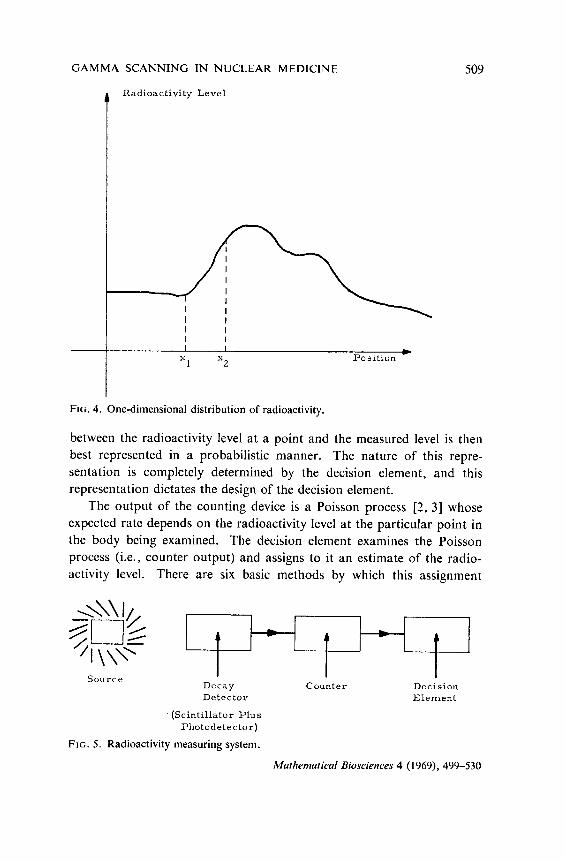
The problems associated with the mapping of the radiation level in

a body can be described with the aid of Figs. 4 and 5. Let Fig. 4 represent

the one-dimensional distribution of radioactivity in a body. The device

for measuring the radioactivity at a particular point, say x, in the body will

generally consist of a radiation detector, which detects the decay of

radioactive particles; a counting system, which counts the number of

decays; and a decision element, which interprets the counter output and

translates it into a radioactivity level. The block diagram of such a

system is shown in Fig. 5.

Suppose that the counter has been set to zero and the radiation

detector has been positioned over the point x1 as indicated in Fig. 4. The

number of radioactive decays is counted (for either a fixed or variable

time) and translated into a radioactivity level by the decision element.

The counter is then reset to zero, the radiation detector moved to a new

point, say x.,, and the radioactivity level at this point is measured. The

device continues until the radioactivity levels at all positions are measured.

Apparently, the ideal measurement device would exactly reproduce the

curve in Fig. 4; however, because of the probabilistic nature of radio-

active decay, such a device is impossible to construct. The relationship



t

Radioactivity Level

FIG. 4. One-dimensional distribution of radioactivity.

between the radioactivity level at a point and the measured level is then

best represented in a probabilistic manner. The nature of this repre-

sentation is completely determined by the decision element, and this

representation dictates the design of the decision element.

The output of the counting device is a Poisson process [2, 31 whose

expected rate depends on the radioactivity level at the particular point in

the body being examined. The decision element examines the Poisson

process (i.e., counter output) and assigns to it an estimate of the radio-

activity level. There are six basic methods by which this assignment

Detector Element

(Scintillator Plus Photodetector)

Frc. 5. Radioactivity measuring system.

Muthemutical Biosciences 4 (1969), 499-530

510 HENRY S. KATZENSTEIN ef al.

might be made. Other techniques as well as hybrid combinations of

these six will now be discussed.

Multilevel Decision Elements (Quantizers)

The first class of decision elements are quantizers of the multilevel

type. It is apparent from Fig. 4 that there is a continuum of radioactivity

levels. From an engineering standpoint, distinguishing between all of

these levels is impractical. For this reason, it is best to consider only

discrete levels of radioactivity. That is, all activity levels I. that lie in the

Typical Counter

T Time t

FIG. 6. Fixed-time decision element.

interval ii < 3, < 3.,+1 (where & and &+, are fixed levels) are assumed to

be at level (;ii + &+,)/2. Theoretically, this discrete approximation to

the continuous curve can be made as close as desired by increasing the

number of levels.

Consider a fixed-time multilevel decision element. The characteristics

of such a device can be explained with the aid of Fig. 6. Consider a

position x in the body with an average radiation level of 1 decays per

second (Poisson process). A count of radioactive decays is made by the

counter for a fixed period of time T. The output of the counter at time T,

say z*, will lie in some interval zi Q z* < z+~. Let 1 be the discrete

output of the decision element, which is considered to estimate /I (the

number of counts or decays per second for the position being examined).

Mathematical Bioscienres 4 (1969), 499-530

GAMMA SCANNING IN NUCLEAR MEDlCINE

Choose a (given zi < z* < zi+J as

511

IL = zi+l + zi

2T

(a is, of course, only an estimate of the true value A).

Having obtained a value of 1 for each point in the body, it is then

possible to construct a picture of the distribution of radioactivity. This

may be done by assigning to each fl a shade of gray. Corresponding to

counter output

z*

t Tl Tz TX T4 T5 T6 T7

Typical Counter Output

FIG. 7. Fixed-count decision elements.

each point in the body, a spot may be made on a flat recording surface

with the color gray corresponding to the estimate fl in the body at that

position. The result is, of course, a “picture” of the radiation level.

The two disadvantages of this scheme are (1) a fixed time is used to

distinguish the radioactivity level at every point (a significant saving in

time can be had by making the time interval variable, as in the multilevel

threshold technique described subsequently); and (2) it is generally

difficult to maintain the various decision levels zi using simple electronic

equipment (i.e., if several levels zi are used, the loss of accuracy due to

drift may be a problem).

A jixed-count multilevel decision technique, which is similar to the

preceding one, can be described by Fig. 7. In this technique the Poisson

process at a point x is monitored until its count exceeds a given level z*


512 HENRY S. KATZENSTEIN et a/.

This takes place at some time T where, for a given set of Ti, Ti < T <

ri-11. The estimate j of the expected decay rate ;1 is then determined as

As in the fixed-time technique, 1 is a random variable and gives only an

estimate of the radioactivity level A at the point. Generation of a picture

from these measurements would be the same as for the fixed-time tech-

nique. The disadvantages of this technique are (1) several decision levels

A counter output

Threshold

c Time

FIG. 8. Multilevel threshold decision element.

(in time) must be maintained without significant drift; and (2) a very

large amount of time might be spent in waiting for the counter outputs to

exceed z* (radioactivity levels corresponding perhaps to a low background

level would take a long time to exceed z*).

The third multilevel decision element, a threshold device, can be

described with the aid of Fig. 8. The “picture” of the radioactivity level

in the body again would be produced by printing spots with various shades

of gray, which represent measured radioactivity levels. Two thresholds

(which are linear with time) are chosen as shown in the figure. As soon as

the counter output crosses either one of the two thresholds, a decision is



made as to the level of radiation at that position in the body being

examined. If the counter output at the crossing point is z and the crossing

time is T, then the estimate fl of the time average decay rate is taken as

fi= zi+1 + zi 7;:+1+ K

where zi < z < z~+~ and Ti < T < Ti+l. This defines a radioactivity 1

(an estimate of the true value) at the point and a spot with a corresponding

shade of gray is then printed. The reason for introducing the two thresh-

olds is to ensure that a sufficiently reliable sample is taken before an

estimate of 1 is made.

The last technique appears to be much more promising than the first

two techniques and probably deserves further study. This report includes

a study of two-level decision elements only.

Two-Letlel Decision Elements

Two-level decision elements are of interest since they are simple to

construct and operate. We consider three such elements in the following

paragraphs.

One possible binary (two-level) technique (which is a special case of

the fixed-time multilevel technique) can be described with the aid of Fig. 9.

The “picture” of the radioactivity pattern is generated in this technique as

follows. At a particular point on the recording surface corresponding to a

point x, either a black spot is recorded or it is not. If an analogy is made

to the fixed-time multilevel technique, there are two shades of gray:

black and white. The picture then is generated by the density of points

rather than by shades of gray. The decision whether or not to print a spot

at a particular position is made on the basis of the counter output z at a

fixed time T. If this quantity exceeds a critical decision level, a spot is

printed. If not, then nothing is printed. The transfer function of this

device is apparently probabilistic in nature. This type of element is

discussed in more detail in a later section. The disadvantage of this

technique is that for each position, a fixed amount of time is necessary to

make a decision, whereas it might be possible to make an adequate

decision in much less time for certain extreme activity levels.

A binary technique that is similar to the preceding one (see Fig. 10)

is now described. Tndeed, it is a special case of the fixed-count multilevel

technique. The counter output continues until it exceeds some fixed

level z*. If the time it takes for z* to be attained is less than some critical


HENRY S. KATZENSTEIN er al. 514

counter Output

-

- Critical Decision

Level

T Time

FIG. 9. Two-level fixed-time decision element.

I

I FIG. 10. Two-level fixed-count decision element.

Matlrernntical Biosciences 4 (1969), 499-530

Critical Decision Time

Time

GAMMA SCANNING 1N NUCLEAR MEDICINE 515

decision time, a spot is printed. If not, no spot is printed. This technique

has basically the same disadvantage as the fixed-time technique in that it

may not be necessary to attain a given count level z* in order to make an

adequate decision about the radioactivity level at a point in the body.

Another binary decision element can be formed as a special case of

the multilevel threshold element. Consider Fig. 11. In this technique

FIG. 11.

Upper Threshold

* Time

Two-level threshold decision element.

two thresholds (which are linear with time) are chosen, as shown in the

figure. The$rst time that the counter output crosses either threshold, a

decision is made. The technique of generating a picture of the radioactivity

is the same as for the other two binary decision elements. That is, the den-

sity of spots generates the picture. If the counter output crosses the

upper threshold, then a spot is printed and the detector moves on to the

next sample point in the body. If the lower threshold is crossed, then no

spot is printed and the detector moves on. There is, of course, always

the possibility that neither threshold will be crossed. In a practical design,

this possibility is handled by terminating any measurement whenever a



maximum measuring time has been exceeded and nothing is printed.

The advantage of this technique over the fixed-time and fixed-count

techniques is that a decision on the radioactivity level can be reached

much more quickly in most cases. This is particularly true of extreme

(high or low) radiation levels. (That this is true will be justified later.)

The disadvantage of this technique is that two thresholds must be gener-

ated and maintained.

4. BINARY FIXED-TIME SCANNING

It is assumed that there is a binary source of radiation that emits

at an average intensity of either A, or AZ (A, > A,) counts per unit time.

It is agreed to observe the source for T seconds, at which time there will

be n counts. The selected decision rule is as follows.

If n > n,, decide that AZ is the source intensity;

if n < n,, decide that ii, is the source intensity;

where n, is such that (P,(X) denotes the probability of the event x)

Pl(n,, T) = Pz(ne, T) (1) and

Pi(n, T) = P, [n counts observed in T seconds given

that the source intensity is A,].

Since the sources are from a radioactive decay, it is known that the

Poisson model is accurate [2], thereby giving

P,(n, T) = (n,T)” exp(-&T). n. 1

Thus, Eq. (1) becomes

(A, T),Q - exp(--IiT) = WF exp(-&T).

n,! n, !

Consequently, the condition on n, becomes

;i;C exp(--I,T) = $cexp(--A,T) or

Taking logarithms,

(2)


GAMMA SCANNING IN NUCLEAR MEDICINE

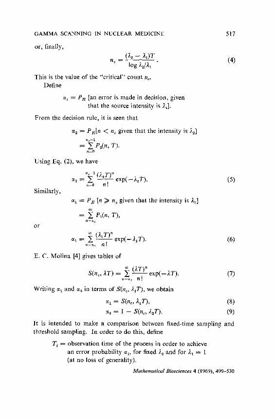
or, finally,

n, = (A2 - m-. log Wl

517

(4)

This is the value of the “critical” count n,.

Define

CQ = P, [an error is made in decision, given

that the source intensity is Ai].

From the decision rule, it is seen that

CI~ = P,[n < n, given that the intensity is AZ]

Q-1

= 2o&h v.

Using Eq. (2), we have

u2 = :z: (+ exp( - h,T). (5)

Similarly,

Ml = P, [n 2 n, given that the intensity is AJ

=.$ P,(n, T), c

or

ccl =ng y exp(--l,T). (6) E .

E. C. Molina [4] gives tables of

S(ner AT) = 2 O”exp(-AT). n=71c n!

Writing c(~ and a2 in terms of S(n,, Air), we obtain

Zl = S(% &T), (8)

a2 = 1 - S(n,, AJ). (9)

It is intended to make a comparison between fixed-time sampling and

threshold sampling. In order to do this, define

Tj = observation time of the process in order to achieve

an error probability xi, for fixed I, and for A, = 1

(at no loss of generality).


518 HENRY

Then define the average observation time T as

T, + TI:, T=-------” 2 .

S. KATZENSTEIN et al.

(10)

In Fig. 12 are shown the results of such calculations for i; using Eqs. (4),

(8), (9), and Molina’s tables, for various 1, and a,; a1 = GC~ = c( has been

chosen in all curves shown, as a means of standardizing the error.

It is necessary to plot a transfer function for this fixed-time method

in order to evaluate its performance for a continuous range of values for

1. Therefore, a plot of the probability of printing a point as a function of

i is made. For any ;1 and T it is observed that the expected value E(n)

of the count n will be E(n) = AT. Therefore, n, = ACT or 1, = n,/T is

obtained. Thus the critical intensity 2, (using Eq. (4)) will be

2 e

= 2, - 21

log ?.,/A, * (11)

Letting ?., = 1 for normalization purposes, Eq. (11) then yields

i, exp(--ii,) = ii, exp(-1,). (12)

Any pair (A,, 1,) satisfying Eq. (12) will give the same value for prob-

abilities of printing a black spot. That is, with probability I - t(2 black

is printed if 1 = )LZ, and with probability a1 black is printed if i = 2,.

For any T then, we obtain a transfer function as required. The results of

this calculation are shown in Fig. 13. These results are compared to those

for binary threshold sampling (Section 5) in Section 6.

5. TWO-LEVEL THRESHOLD DECISION ELEMENT (VARIABLE TIME)

In this section some of the more important properties of the two-level

threshold decision elements are discussed and analyzed. This element was

explained earlier with the use of Fig. 11, which is also pertinent to the

discussion in this section.

If the two-level threshold decision element is used, the picture of the

radiation pattern is generated by varying the density of black spots on a

recording surface. Regions of high, medium, and low spot densities

correspond to high, medium, and low radioactivity levels, respectively.

The decision whether or not a spot is printed at a particular point depends

on whether the counter output crosses the upper or lower threshold.

Since these crossings are probabilistic in nature, the pattern will be

somewhat random in nature. For example, even though the radioactivity


GAMMA SCANNING IN NUCLEAR MEDICINE

FIG. time

VERTICAL AXIS: NORMALIZED EXPECTED 32 - DECISION TIME n/l,

HORIZONTAL AXIS: PROBABILITY OF ERROR

30 - a (a,= cl2’ca)

28 -

26 -

24 -

0 0.02 0.04 O.O~O.lO 0.12 0.14 0.16 0.113

519

12. Relationship between average decision time and error probability for fixed-

element.



I I I I I I I I I

Probability of Printing a Spot

Mathematical Biosciences 4 (1969)) 499-530


level at a particular point is very high, the counter output may cross the

lower threshold and no spot will be printed. If measurements are made

at many points in a region with a high radioactivity level, then the prob-

ability of spots being printed for many of these points will be high. The

nature of this decision element cannot be completely described by a simple

decision rule that relates the radioactivity level and the corresponding

decision whether or not a spot is printed. Instead it must be described by

a representation (referred to as a transfer function) that relates the

radioactivity level and the probability that a spot is printed. Such a

representation has been shown in Fig. 13 (for fixed-time sampling). It is

apparent that above a certain radioactivity level, say 1, the probability

of a spot is essentially unity. These decision elements cannot practically

distinguish (probabilistically) between various levels above the level 1.

Another variable of importance in this technique is the time it takes to

reach a decision whether a spot should be printed or not. It is desirable

to make the decision time as short as possible without excessively degrading

the accuracy of the decision.

If the radioactivity level is constant over a region and measurements

are made at a large number of points in this region, then the density of

spots should be approximately equal to the probability of a spot for that

radioactivity level. The transfer function might then be considered to be

the transfer function between radioactivity level and spot density. It is

probably desirable for such a transfer function to be approximately

linear; however, without additional knowledge about the averaging and

smoothing properties of the human eye, this is only conjecture.

It is clear that two important properties of the binary threshold tech-

nique are (1) the expected time needed to reach a decision at each point

in the body; and (2) the ability to distinguish accurately between two

fixed radioactivity levels. As might be expected, these two properties are

not independent. That is, the expected time to reach a decision, the

accuracy of the decision (in a probabilistic sense), and the radioactivity

levels are functionally related.

To generate (graphical) relationships that describe the properties of

the binary threshold decision element, the theory of sequential hypothesis

testing [5-81 has been used. The problem of sequential hypothesis testing

can be defined as follows [7, 81.

Let {zl(t), t > 0} and {zz(t), t > 0} be two different stochastic

processes. An observer, beginning at t = 0, continuously monitors


35


a stochastic process {z(t), t > O> that is either {zl(t)} or {zz(t)> and

wishes to decide, as SOOT as possible, whether {z(t)} is {zl(t)} or {zz(t)}.

The phrase “as soon as possible” is defined as follows. Let T be the

time when a decision is reached. T is clearly a random variable. Let

E,(T) and E,(T) be the expected values of T when {z(t)} = {zl(t)} and

(z(t)} = {zz(t)}, respectively. Let tll and CQ be two positive constants

such that CI~ + u2 < 1. If the restriction is made that the probability

of an incorrect decision when {z(t)} = {zi(t)} is fixed at xi, then the

problem is to find a procedure for deciding between {zi(t)} and {zz(t)}

such that El(T) and E,(T) are minimized, given CQ and Q.

In this writing, the two processes {zl(t)} and {zz(t)} are assumed to be

Poisson processes with stationary independent increments and mean

occurrence times l/1, and l/1,, respectively. This model was described

in Section 2. The problem in this case is deciding whether or not the

mean occurrence time of the observed process is l/d, or l/n,. The

optimal test procedure (in the sense that E,(T) and E2(T) are minimized

for fixed or and CCJ is given by a Wald sequential probability ratio test

[5,61. More specifically, let z(t) be the observed process and define

Z(t) = z(t) log $ - (a2 - a& 1

where L, > il,. Then the best decision rule is specified by two numbers,

a, b (b < 0 < a) in the following manner. As long as I(t) lies between a

and b, observation of z(f) continues. As soon as Z(t) < b, stop observing

{z(t)} and decide I = 3L1. As soon as Z(t) > a, stop observing {z(t)} and

decide 3, = 2,. Now for any other procedure with error probabilities ct:

and u,* and expected decision times E,*(T) and E,*(T), then CC: < CQ,

CX,* < tc2 implies Et(T) > E,(T) and E:(T) > E,(T). Figure 14 is a

sketch of how this type of decision rule works. In this case, the process

I(t) crosses the decision level at a time t, and at that time it is decided that

L = 2,.

To put this decision rule into the form of the binary threshold decision

rule, it should be noted that b Q l(t) < a implies that



“0 I

FIG. 14. Sketch of decision function.

Now let

Then the two linear time functions

J + @, - 4)t

log &I&

and K + (& - 4)t

log &I&

are, respectively, the upper and lower thresholds of the two-level threshold

decision rule; Fig. 11 is a sketch that illustrates this type of decision rule.

The values for J and K are completely determined by the values A,, A.,,

a, and b. The values for a and b are calculated from the given error

probabilities CI~ and tcz. In particular,

and

b = log -2% 1 - ctl

1 - c?z log? + log-

1 -a2 < a Q log - .

2 Nl El

Note that a is not uniquely given by these expressions, but is merely

bounded from above and below. There are no simple analytic expressions



for J and K that can be used for design purposes due to the difficulty in

uniquely specifying a; in [8], however, tables have been prepared that

relate il,, AI, x3, x1, J, K, E,(T), and E,(T). Using these tables, it is

possible to fix certain of these variables and determine from the tables

the values of the remaining variables. For instance, if &, AI, Q, and c(r

are specified then J, K, E,(T), and E,(T) have fixed values that can be

determined from these tables. Or, if J, K, &, and iI are specified, then

r.1, $3 E,(T), and E,(T) have fixed values that can be determined from

these tables.

Using these tables, curves have been plotted in Fig. 15 that represent

the relationship among the expected time to reach a decision, the radio-

activity levels A1 and A,, and the probabilities of errors scr and C+ Since

it is difficult to represent the dependence of all these quantities in a

reasonable graphical form, the relationships have been somewhat simpli-

fied by making certain assumptions. It is assumed that c(t = tlZ = o!

and that the processes defined by A1 and AZ are equally likely. This

second assumption allows us to define an average time of decision as

In addition, it is intuitively apparent (and can be shown rigorously) that

the time to reach a decision varies inversely as the radioactivity levels.

For example, let 3,, = 1, &/A1 be fixed, and A be the corresponding

expected time to reach a decision; if A1 = 2 and &/Al has the same value,

the expected time to reach a decision is x/2. Figure 16 is then a family of

curves of the normalized expected time versus the probability of error tc

with the ratio 3.,/A, as the parameter. These curves can be used in either

of two ways. First, suppose &/I., is fixed and it is desired to determine

how much time it takes to make a decision with expected error CC Find

the given value of I on the abscissa and go vertically from this value to the

intersection with the curve defined by the given ?,,/A,. The expected

decision time is then the ordinate of this intersection. The second way in

which this family of curves can be used is as follows. Let a be a fixed

expected error and 2 be a fixed decision time. The intersection of these

two values will lie on a member of the family of curves and therefore fix

the ratio AZ/A1 = I.*. That is, for a given time and given allowable error

the decision element can distinguish between levels A1 and A, only if

/?,/A, > ;I”.



I I I I I I

Probability of Errors a (aI = a2 = d

FIG. 15. Relationship between expected decision time and error probability for threshold element.



h4athematical Biosciences 4 (1969), 499-530


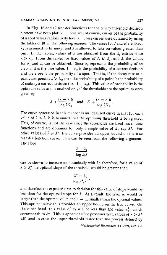
In Figs. 16 and 17 transfer functions for the binary threshold decision

element have been plotted. These are, of course, curves of the probability

of a spot versus radioactivity level 1. These curves were obtained by using

the tables of [8] in the following manner. The values for J and K are fixed,

il, is assumed to be unity, and jl is allowed to take on values greater than

one. In the tables, values of ;1 are obtained from the & entries since

ii > &. From the tables for fixed values of J, K, A,, and ii, the values

for c(i and CI~ can be obtained. Since a2 represents the probability of an

error if A is the true value, 1 - a2 is the probability of a correct decision

and therefore is the probability of a spot. That is, if the decay rate at a

particular point is jl > A,, then the probability of a point is the probability

of making a correct decision (i.e., 1 - CQ). This value of probability is the

optimum value and is attained only if the thresholds are the optimum ones

given by

The curve generated in this manner is an idealized curve in that for each

value of L > 2, it is assumed that the optimum threshold is being used.

This, of course, is not the case since the thresholds are fixed linear time

functions and are optimum for only a single value of &, say A*. For

other values of 1 # A*, the curve provides an upper bound on the true

transfer function curve. This can be seen from the following argument.

The slope

can be shown to increase monotonically with 1; therefore, for a value of

L > 2; the optimal slope of the threshold would be greater than

and therefore the expected time to decision for this value of slope would be

less than for the optimal slope for A. As a result, the error CQ would be

larger than the optimal value and 1 - CI~ smaller than the optimal values,

This optimal curve thus provides an upper bound on the true curve. On

the other hand, this value of aZ will be less than the value a,*, which

corresponds to ;2*. This is apparent since processes with values of il > 1*

will tend to cross the upper threshold faster than the process defined by


13

.i i

!//

ii -

1”

A

.i i

K

--i

x J

ii--,

0 ;

z 2

K_

-_L

IIII

I 1

2.53

3.54

5

7 0.

25

0.

‘3,

0. j*

,s

0.

it38

! -I I

FIG

. 17

. T

rans

fer

func

tion

for

bina

ry

thre

shol

d de

cisi

on

elem

ent

(asy

mm

etri

cal

thre

shol

d).


?,*. This optimal transfer function then provides both upper and lower

bounds on the true transfer function.

For those values of 1 such that il < 1 a dual argument is used to

generate that portion of the idea1 transfer function. Similar upper and

lower bounds on the time transfer function can also be generated in

similar ways. A number of these curves have been plotted for various

values of J and K in order to get an idea as to the dependence of the

transfer function on these parameters.

6. COMPARISON OF BINARY FIXED-TIME AND THRESHOLD SCANNING

In Sections 4 and 5, the binary fixed-time and binary threshold

(variable time) scanning procedures, respectively, were analyzed. A

comparison of the performance of these two systems is now presented.

The significant measure of performance for these two systems is

contained in the plot of the family of average scan times versus error

probability with il,/jl, as a parameter (Figs. 12 and 15). It is seen im-

mediately that, for a given &/jll and cc, 2 m T/‘/2, which indicates that at

the same binary source intensities and at the same error probabilities,

the threshold system will take approximately one half as long a scan time

as the fixed-time system. Alternatively, we see that for a given average

scan time and a given error probability, the required ratio AZ/Al is always

larger for fixed-time sampling (the relative difference depends on the

particular values used). Lastly, for a given average scan time and given

&/A,, the threshold scanning is seen to be significantly superior to the

fixed-time sampling in terms of probability of error (ratios as large as 10: I

are easily found).

The transfer functions for both systems are given in Figs. 13 and 16.

The only pertinent statement here is that both systems provide enough

degrees of freedom to allow a variety of transfer functions to be chosen.

In the fixed-time case, the parameter is T, the transfer function becoming

sharper as T increases. In the threshold scanning method, the parameters

are J and K, where J - K is merely the vertical height separating the

two parallel linear thresholds; as J - K increases, the transfer function

becomes sharper. If the transfer function is chosen to be relatively flat,

then boundaries separating high- and low-intensity regions will be wide and

relatively indistinct. On the other hand, if the slope is steep, then the

boundaries will be sharp, but the gray levels will be suppressed. An

optimum choice here depends on the medical investigator’s purposes.



7. EXPERIMENTAL PROGRAM

An experimental program to develop a sequential sampling computer

and to evaluate it in conjunction with a gamma scanner has been under-

taken. (This work was supported by the Division of Biology and Medi-

cine, U.S. Atomic Energy Commission, under contract AT(04-3)-627.)

The preliminary results have been reported elsewhere [9]. A final report,

for publication, is in the process of preparation [lo].

REFERENCES

1 W. H. Blahd, N&ear medicine, pp. 263-288. McGraw-Hill, New York, 1965. 2 W. Feller, An introduction to probability and its applications, Vol. I. Wiley, New

York, 1957. 3 J. L. Doob, Stochasticprocesses. Wiley, New York, 1953. 4 E. C. Molina, Poisson exponential binomial limit. Van Nostrand, Princeton, New

Jersey, 1942. 5 A. Wald, Sequential tests of statistical hypotheses, Ann. Math. Stat. 16(1945),

117-186.

6 A. Wald, Sequential analysis. Wiley, New York, 1947. 7 A. Dvoretzky, J. Kiefer, and J. Wolfowitz, Sequential decision problems for proc-

esses with continuous time parameter testing hypotheses, Ann. Math. Stat. 24 (1953),

254-264.

8 J. Kiefer and J. Wolfowitz, Sequential tests of hypotheses about the mean occurrence time of a continuous parameter Poisson process, Naual Res. Logs Q. 1957,205-219.

9 H. S. Katzenstein, Application of sequential sampling analysis to radioisotope scan-

ning, Paper O-7 presented at meeting of Sot. Nuclear Med. (Seattle, Washington), June 20-23, 1967.

10 H. S. Katzenstein and P. Jensen, Application of sequential sampling analysis to the

improvement of medical scanning; to be submitted to J. Nuclertr Med.


mathematical biosciences 499 application of the ... of the... · mathematical biosciences 499...

Documents